Operating Systems / Betriebssysteme - Baun C.

2
Fundamentals of Computer Science
2.1
Bit

2.2.1
Decimal System
2.2.2
Binary System

3 Fundamentals of Operating Systems
3.1
Operating Systems in Computer Science

3.2
Positioning and Core Functionalities of Operating Systems

3.4
Operating Modes
3.4.1 Batch Processing and Time-sharing

3.6
Real-Time Operating Systems
3.6.1
Hard and Soft Real-Time Operating Systems

3.6.2
Architectures of Real-Time Operating Systems

3.8.1
Monolithic Kernels
3.8.2
Microkernels

3.9
Structure (Layers) of Operating Systems

4
Fundamentals of Computer Architecture
4.1
Von Neumann Architecture

4.4.6
Addressing Data on Hard Disk Drives

4.4.7
Access Time of HDDs
4.4.8
Solid-State Drives

4.4.9
Reading Data from Flash Memory Cells

5
Memory Management
5.1
Memory Management Concepts

5.2.3
Page-based Memory Management (Paging)

5.2.4
Segment-based Memory Management (Segmentation)

5.2.5
State of the Art of Virtual Memory

6
File Systems
6.1
Technical Principles of File Systems

6.2
Block Addressing in Linux File Systems

6.3
File Systems with a File Allocation Table

6.7
Accelerating Data Access with a Cache

7
System Calls
7.1
User Mode and Kernel Mode

8
Process Management
8.1
Process Context

8.6
Process Switching and Process Scheduling

8.6.4
Shortest Job First / Shortest Process Next

8.6.6
Longest Job First
8.6.7
Longest Remaining Time First

8.6.8
Highest Response Ratio Next
8.6.9
Earliest Deadline First

8.6.12
Scheduling of Linux Operating Systems

9
Interprocess Communication
9.1
Critical Sections and Race Conditions

9.2.1
Specification of the Execution Order of Processes

9.2.2
Protecting Critical Sections by Blocking

9.3
Communication of Processes
9.3.1
Shared Memory (System V)

9.4
Cooperation of Processes
9.4.1
Semaphore according to Dijkstra

10.7
Operating System-level Virtualization

Author: Baun C.

Tags: operating systems betriebssysteme

ISBN: 978-3-658-42229-5

Year: 2023

Similar

Linux-Unix-Systemprogrammierung

BIOS: Optimales Hardware-Setup

Windows Internals. Band 1: Systemarchitektur, Prozesse, Threads, Speicherverwaltung, Sicherheit und mehr

PC-Hardwarebuch Aufbau, Funktionsweise, Programmierung Ein Handbuch nicht nur für Profis

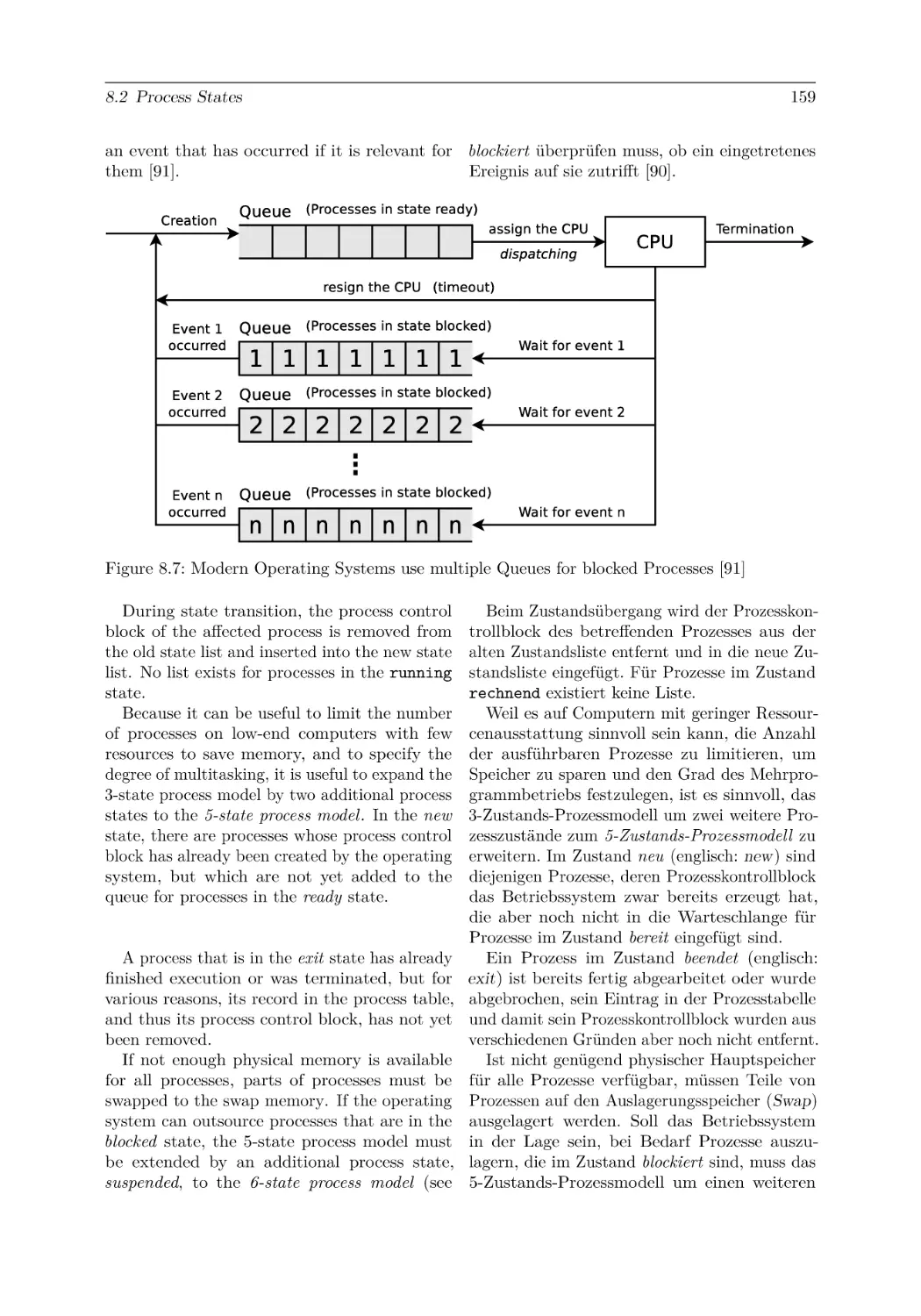
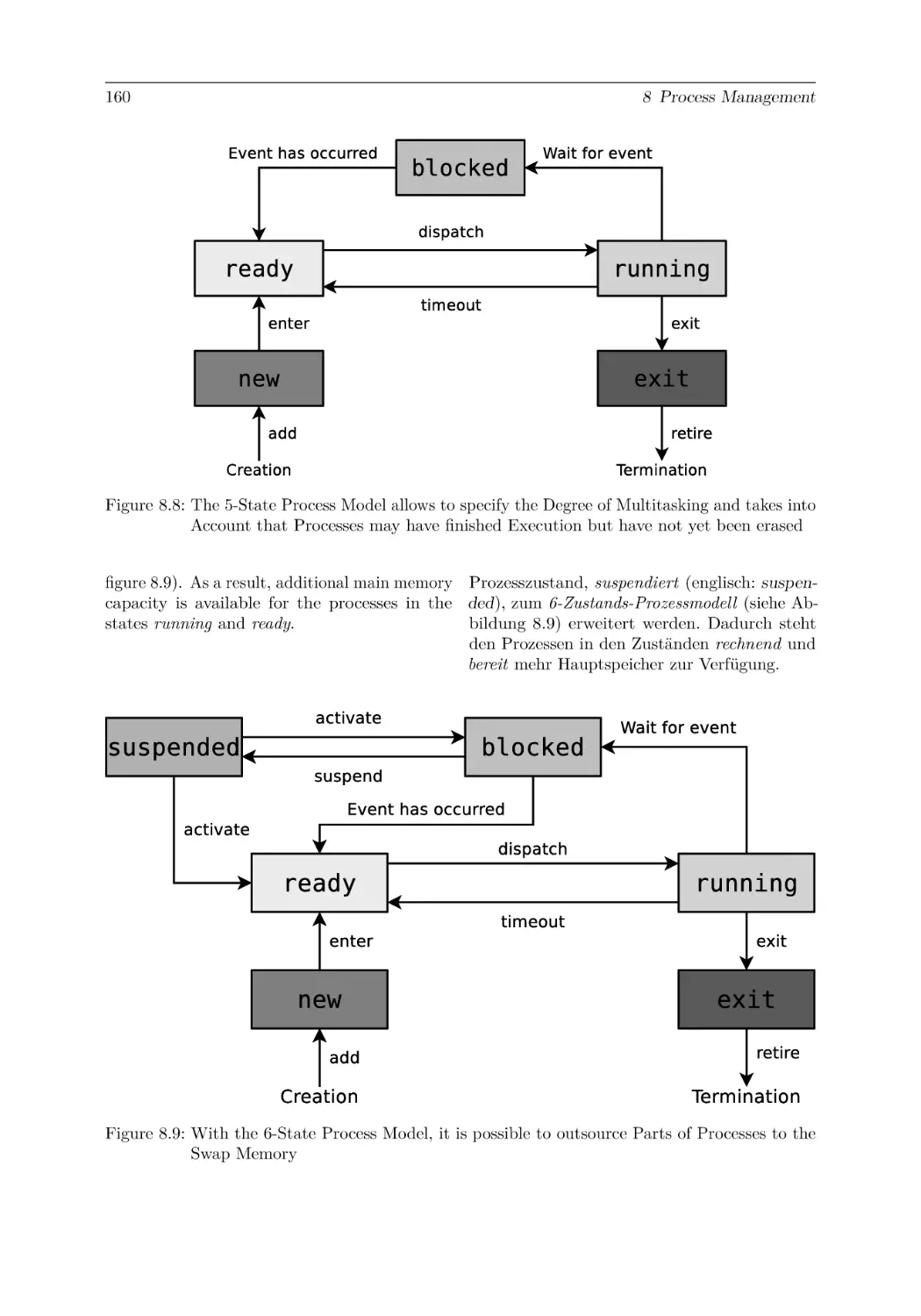
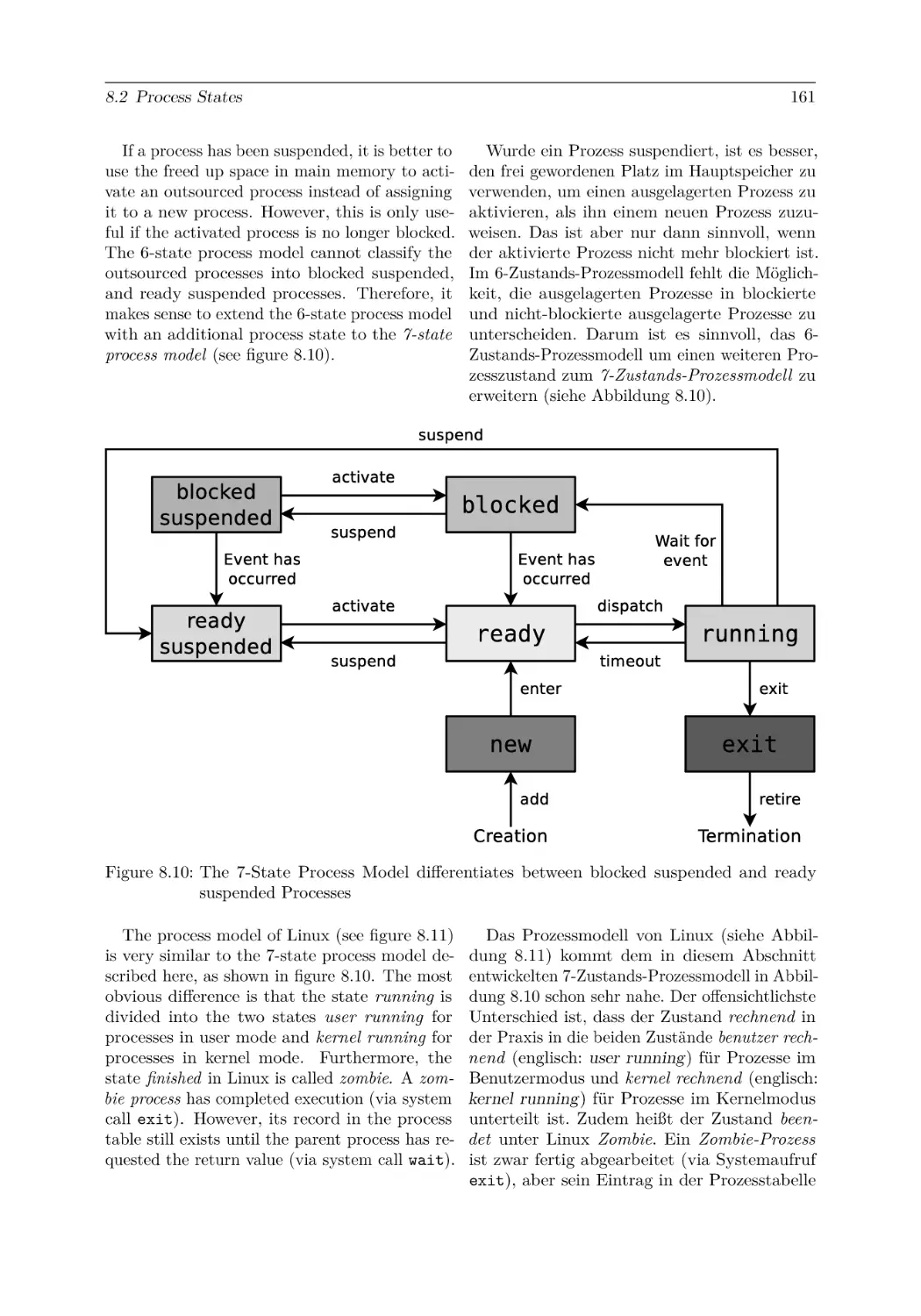
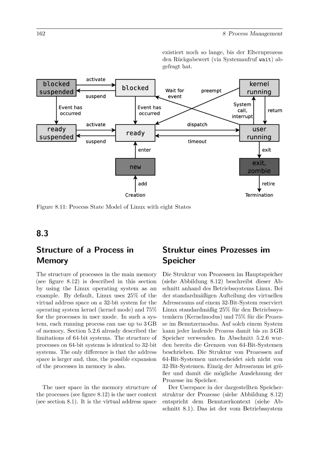
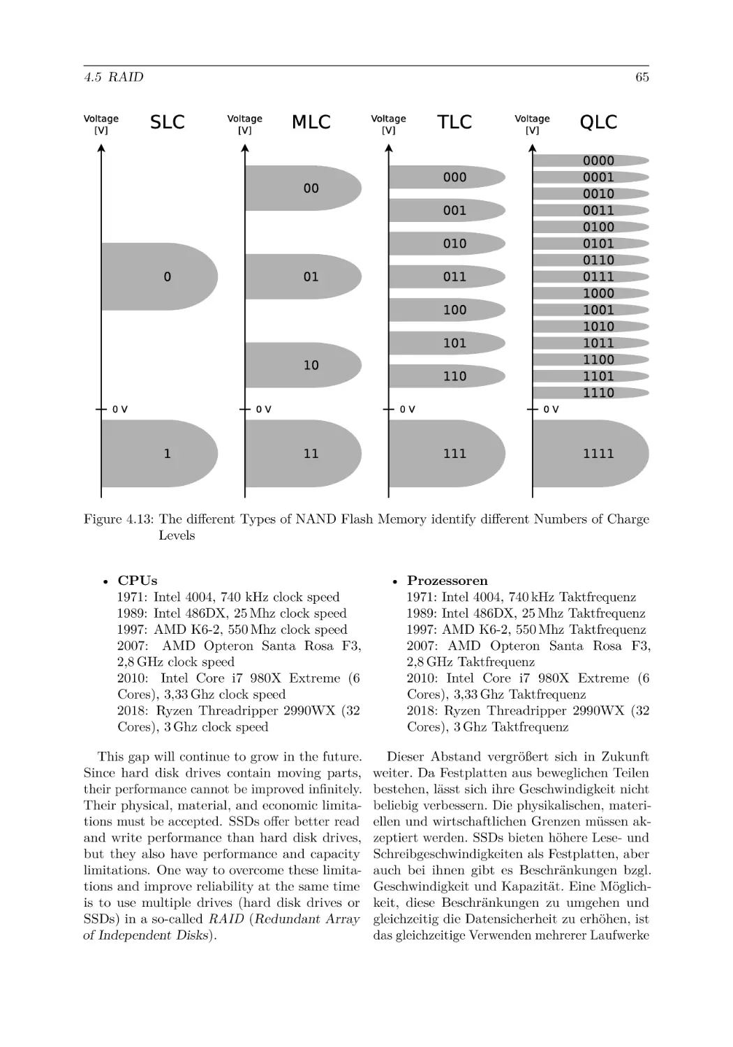
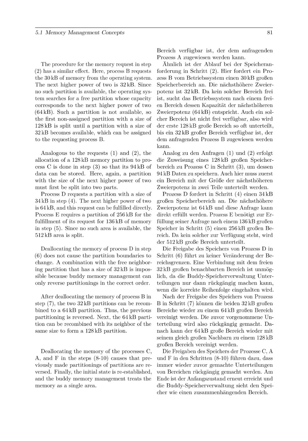
Text

Christian Baun

Operating Systems/
Betriebssysteme
Bilingual Edition: English – German/
Zweisprachige Ausgabe: Englisch – Deutsch
2nd edition/2. Auflage

Operating Systems / Betriebssysteme

Christian Baun

Operating Systems /
Betriebssysteme
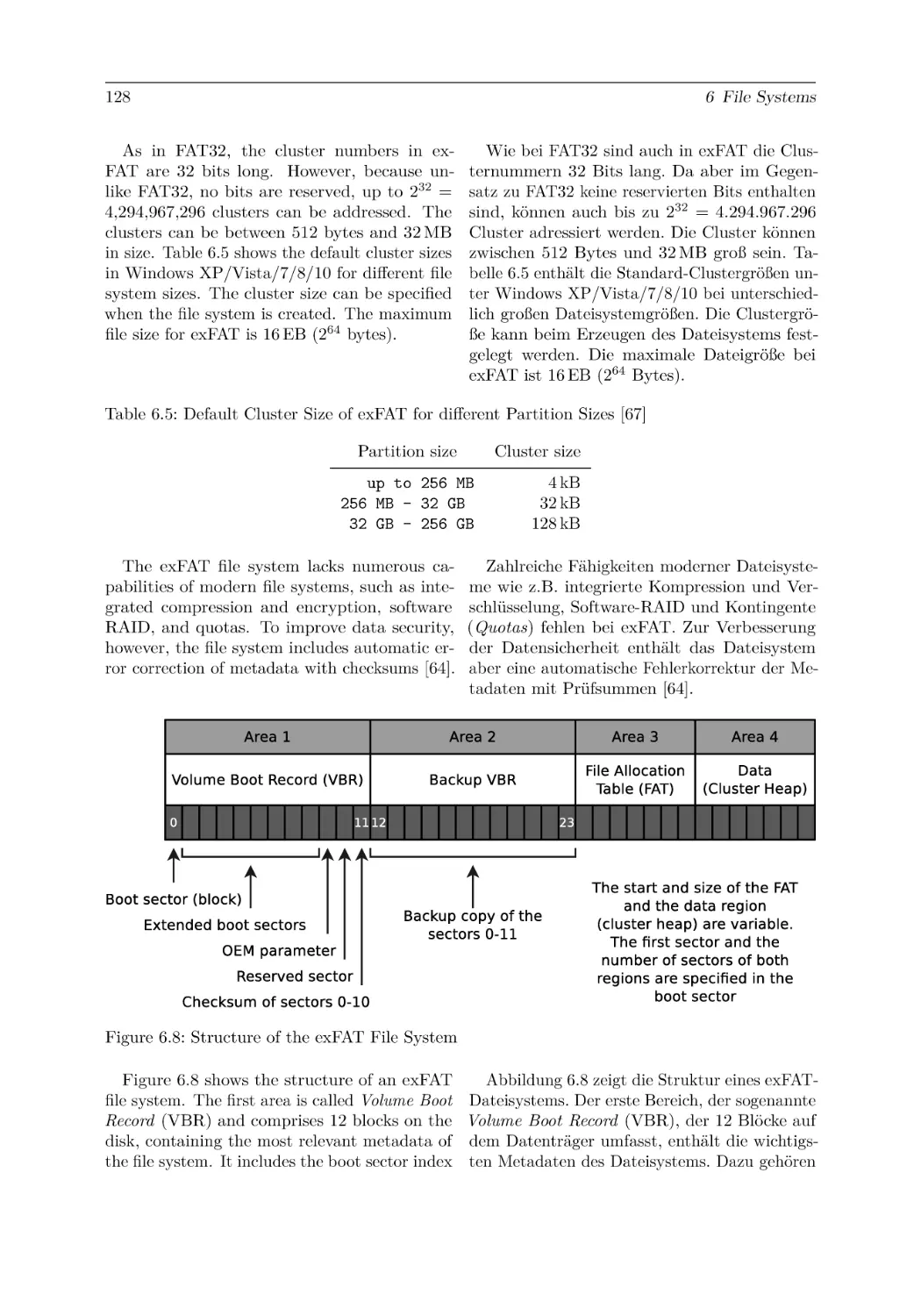
Bilingual Edition: English – German /
Zweisprachige Ausgabe:
Englisch – Deutsch
2nd edition/2. Auflage

Christian Baun
FB 2
Frankfurt University of Applied Sciences
Frankfurt am Main, Deutschland

ISBN 978-3-658-42229-5
ISBN 978-3-658-42230-1 (eBook)
https://doi.org/10.1007/978-3-658-42230-1
Die Deutsche Nationalbibliothek verzeichnet diese Publikation in der Deutschen Nationalbibliografie; detaillierte
bibliografische Daten sind im Internet über http://dnb.d-nb.de abrufbar.
© Springer Fachmedien Wiesbaden GmbH, ein Teil von Springer Nature 2020, 2023
Das Werk einschließlich aller seiner Teile ist urheberrechtlich geschützt. Jede Verwertung, die nicht ausdrücklich
vom Urheberrechtsgesetz zugelassen ist, bedarf der vorherigen Zustimmung des Verlags. Das gilt insbesondere für
Vervielfältigungen, Bearbeitungen, Übersetzungen, Mikroverfilmungen und die Einspeicherung und Verarbeitung
in elektronischen Systemen.
Die Wiedergabe von allgemein beschreibenden Bezeichnungen, Marken, Unternehmensnamen etc. in diesem
Werk bedeutet nicht, dass diese frei durch jedermann benutzt werden dürfen. Die Berechtigung zur Benutzung
unterliegt, auch ohne gesonderten Hinweis hierzu, den Regeln des Markenrechts. Die Rechte des jeweiligen
Zeicheninhabers sind zu beachten.
Der Verlag, die Autoren und die Herausgeber gehen davon aus, dass die Angaben und Informationen in diesem
Werk zum Zeitpunkt der Veröffentlichung vollständig und korrekt sind. Weder der Verlag noch die Autoren oder
die Herausgeber übernehmen, ausdrücklich oder implizit, Gewähr für den Inhalt des Werkes, etwaige Fehler
oder Äußerungen. Der Verlag bleibt im Hinblick auf geografische Zuordnungen und Gebietsbezeichnungen in
veröffentlichten Karten und Institutionsadressen neutral.
Planung/Lektorat: David Imgrund
Springer Vieweg ist ein Imprint der eingetragenen Gesellschaft Springer Fachmedien Wiesbaden GmbH und ist
ein Teil von Springer Nature.
Die Anschrift der Gesellschaft ist: Abraham-Lincoln-Str. 46, 65189 Wiesbaden, Germany

Preface to the
second Edition

Vorwort zur
2. Auﬂage

This edition includes some additional topics
Diese Auﬂage enthält einige neue Themen
and some didactical enhancements.
und didaktische Verbesserungen.
Chapter 5 now also describes the ﬁve-level
Kapitel 5 berücksichtigt nun auch das fünfpaging implemented by the latest server CPUs. stuﬁge Paging, das neueste Server-Prozessoren
implementieren.
In chapter 6, the sections about the ﬁle sysIn Kapitel 6 wurden die Abschnitte zu den
tems ext4 and Minix have been expanded. In Dateisystemen ext4 und Minix erweitert. Neu
addition, new illustrations about the structure hinzugekommen sind unter anderem Abbildunof the NTFS ﬁle system, the Master File Table gen zur Struktur des Dateisystems NTFS und
(MFT), and the Copy-on-Write working princi- der Einträge in der Master File Table (MFT)
ple have been added, among other things. Fur- sowie zur Arbeitsweise von Copy-on-Write. Zuthermore, this edition, for the ﬁrst time, con- dem enthält diese Auﬂage erstmals Abschnitte
tains sections about the modern ﬁle systems zu den modernen Dateisystemen exFAT, ZFS,
exFAT, ZFS, Btrfs, and ReFS.
Btrfs und ReFS.
Chapter 8 contains new content about process
Kapitel 8 enthält zum Thema Prozessverwalmanagement for better understanding. Among tung neue Inhalte, die das Verständnis erleichother things, a new illustration of process switch- tern. Unter anderem gibt es eine neue Abbiling and the relationship between user space, dung zu Prozesswechseln und der Zusammenvirtual memory, and user context is better ex- hang zwischen Userspace, virtuellem Speicher
plained in section 8.3. In addition, descriptions und Benutzerkontext ist in Abschnitt 8.3 besser
of process scheduling in Linux operating systems erklärt. Neu sind auch die Beschreibungen des
have also been added in section 8.6.12.
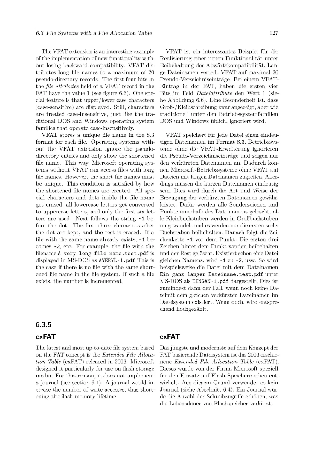
Prozess-Schedulings in Linux-Betriebssystemen
in Abschnitt 8.6.12.
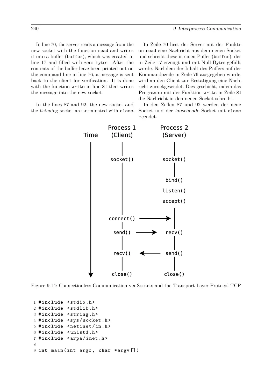
The sections covering interprocess communiErweitert wurden die Themen Interprozesscation and cooperation of processes have been kommunikation und Kooperation von Prozesexpanded in chapter 9. The descriptions of TCP sen in Kapitel 9. Die Beschreibungen zu TCPsockets have been expanded, and examples of Sockets wurden ausgebaut und Beispiele zu
UDP sockets have been added. The descriptions UDP-Sockets sind neu hinzugekommen. Die
of system calls and library functions for interpro- Beschreibungen der Systemaufrufe und Bibliocess communication have been expanded a lot, theksfunktionen zur Interprozesskommunikatiand examples of working with the POSIX inter- on wurden insgesamt ausgebaut und Beispieface for shared memory areas, message queues, le zur Arbeit mit der Schnittstelle POSIX für
and semaphores are new in this edition. Finally, gemeinsame Speicherbereiche, Nachrichtenwarthe section covering the cooperation of processes teschlangen und Semaphoren sind neu in dieand threads with mutexes has been completely ser Auﬂage dazugekommen. Der Abschnitt zur
reworked.
Kooperation von Prozessen und Threads mit
Mutexen wurde komplett überarbeitet.

vi
The command-line instructions for compiling
and running the programs are now included in
the output of the program examples in chapters
7, 8, and 9. This makes it easier for beginners
to follow the individual steps from the source
code to the output of the programs.
Several sections in Chapter 10 have also been
reworked. In particular, the sections covering
the partitioning and the emulators have been
extended.
At this point, I would like to thank my editor
David Imgrund for his support. I would also like
to thank Jörg Abke from the TH Aschaﬀenburg,
Michael Eggert from the Würzburg-Schweinfurt
University of Technology, and Henry Cocos, Peter Ebinger, Oliver Hahm, Benedikt Möller, Anton Rösler, and Amalie-Margarete Wilke from
the Frankfurt UAS for their helpful comments
and suggestions for improvement. Finally, I
thank my wife, Katrin Baun, for her strong
encouragement and support.
Frankfurt am Main
July 2023

Bei den Ausgaben der Programmbeispiele in
den Kapitel 7, 8 und 9 sind die Kommandozeilenbefehle zum Kompilieren und Ausführen nun
mit dabei. Dies erleichtert Einsteigern das Nachvollziehen der einzelnen Schritte vom Quellcode
zur Ausgabe der Programme.
Überarbeitet wurden auch mehrere Abschnitte in Kapitel 10. In erster Linie die Themen
Partitionierung und Emulatoren sind nun inhaltlich erweitert.
An dieser Stelle möchte ich meinem Lektor
David Imgrund für seine Unterstützung danken.
Zudem danke ich Jörg Abke von der TH Aschaffenburg, Michael Eggert von der Technischen
Hochschule Würzburg-Schweinfurt sowie Henry
Cocos, Peter Ebinger, Oliver Hahm, Benedikt
Möller, Anton Rösler und Amalie-Margarete
Wilke von der Frankfurt UAS für hilfreiche Verbesserungsvorschläge. Meiner Frau Katrin Baun
danke ich für das Korrekturlesen und die viele
Motivation und Unterstützung.
Prof. Dr. Christian Baun

vii

Preface to the
ﬁrst Edition

Vorwort zur
1. Auﬂage

Operating systems are an important topic of
practical computer science and, to a lesser extent, also of technical computer science. They
are the interface between the hardware of a
computer system and its users and their software processes. Furthermore, operating systems
manage the hardware components of a computer
system and the stored data.
This compact book on the broad topic of
operating systems was written to provide an
overview of the most essential task areas and
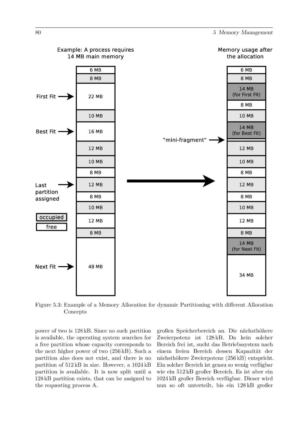
core functionalities of operating systems, and
thus assist the readers in learning how operating
systems work, how they implement essential
functionalities, and how they use and control
the most important hardware components of a
computer system.

Betriebssysteme sind ein wichtiges Thema der
praktischen Informatik und zum geringeren Teil
auch der technischen Informatik. Sie sind die
Schnittstelle zwischen der Hardware eines Computers und seinen Benutzern und deren Softwareprozessen. Zudem verwalten Betriebssysteme
die Hardwarekomponenten eines Computers und
die gespeicherten Daten.
Dieses kompakte Werk über das breite Thema Betriebssysteme wurde mit dem Ziel geschrieben, dem Leser einen Überblick über die
wichtigsten Aufgabenbereiche und Kernfunktionalitäten von Betriebssystemen zu verschaﬀen
und so das Verständnis dafür zu wecken, wie Betriebssysteme funktionieren, wie sie die wichtigsten Funktionalitäten erbringen und wie sie die
wichtigsten Hardwarekomponenten eines Computers nutzen und steuern.
Zudem soll dieses Buch diejenigen Leser unterstützen, die sich nicht nur fachlich im Thema
Betriebssysteme, sondern auch sprachlich in der
englischen oder in der deutschen Sprache weiterbilden möchten.
Die Motivation, dieses zweisprachige Lehrbuch zu schreiben, ergab sich aus den Veränderungen des Hochschulalltags in jüngerer Vergangenheit. Zahlreiche Hochschulen haben einzelne Module oder ganze Studiengänge auf die
englische Sprache umgestellt, um für ausländische Studenten attraktiver zu sein, und um die
sprachlichen Fähigkeiten der Absolventen zu
verbessern.
Die Programmbeispiele in diesem Werk wurden alle in der Programmiersprache C geschrieben und unter dem freien Betriebssystem Debian GNU/Linux getestet. Prinzipiell sollten sie
unter jedem anderen Unix-(ähnlichen) Betriebssystem laufen.
Die Programmbeispiele und die Errata-Liste
wird hier veröﬀentlicht:
https://christianbaun.de
Wenn Ihnen bei der Arbeit mit diesem Werk
Kritikpunkte auﬀallen, oder Sie Verbesserungsvorschläge für zukünftige Auﬂagen haben, würde

Also, this book intends to support those readers who wish to learn not only technical aspects
of operating systems, but also want to improve
their language skills in English or German.
The motivation to write this bilingual textbook arose from recent changes in universities.
Many universities have migrated individual modules or even whole study programs to English
to be more attractive for international students
and to improve the language skills of the graduates.

The example programs in this book were all
written in the C programming language and
tested under the free operating system Debian
GNU/Linux. In principle, they should run under any other Unix-like operating system.
The example programs and the errata list will
be published here:
https://christianbaun.de
If you notice any points of criticism while
working with this book, or if you have suggestions for improvement for future editions,

viii
I would be happy to receive an email from you:
christianbaun@gmail.com
At this point, I want to thank my editor
Sybille Thelen for her support. Also, many
thanks to Turhan Arslan, and especially Jens
Liebehenschel and Torsten Wiens, for proofreading. I thank my parents Dr. Marianne Baun and
Karl-Gustav Baun, as well as my parents-in-law
Anette Jost and Hans Jost and, in particular,
my wife, Katrin Baun, for their motivation and
support in good times and in diﬃcult times.

Frankfurt am Main
März 2020

ich mich über eine Email von Ihnen sehr freuen:
christianbaun@gmail.com
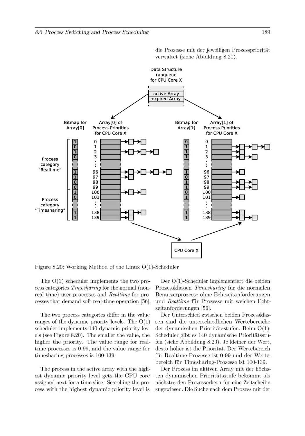
An dieser Stelle möchte ich meiner Lektorin
Sybille Thelen für ihre Unterstützung danken.
Zudem danke ich Turhan Arslan und ganz besonders Jens Liebehenschel und Torsten Wiens
für das Korrekturlesen. Meinen Eltern Dr. Marianne Baun und Karl-Gustav Baun sowie meinen
Schwiegereltern Anette Jost und Hans Jost und
ganz besonders meiner Frau Katrin Baun danke
ich für die Motivation und Unterstützung in
guten und in schwierigen Zeiten.
Prof. Dr. Christian Baun

Contents
1 Introduction
2 Fundamentals of Computer Science
2.1 Bit . . . . . . . . . . . . . . . . .
2.2 Representation of Numbers . . .
2.2.1 Decimal System . . . . . .
2.2.2 Binary System . . . . . .
2.2.3 Octal System . . . . . . .
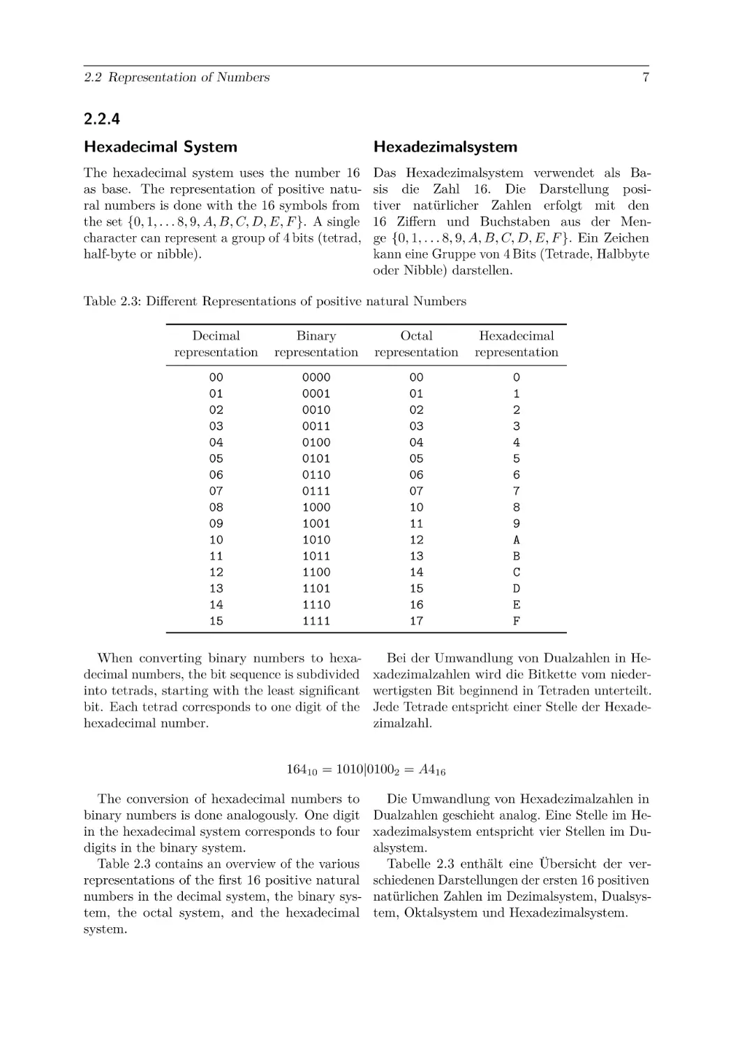
2.2.4 Hexadecimal System . . .
2.3 File and Storage Dimensions . .
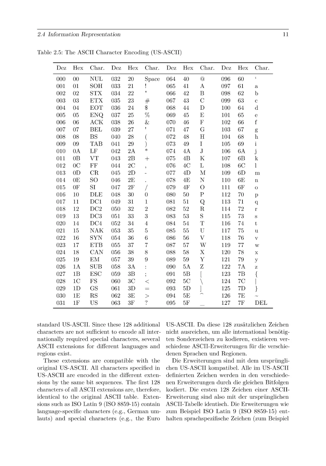
2.4 Information Representation . . .
2.4.1 ASCII Encoding . . . . .
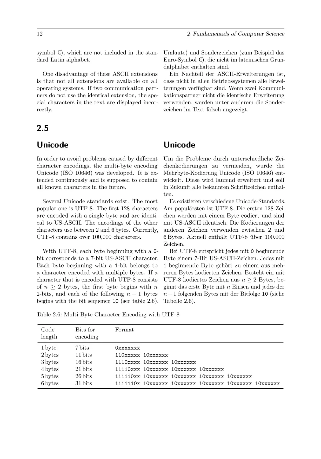
2.5 Unicode . . . . . . . . . . . . . .
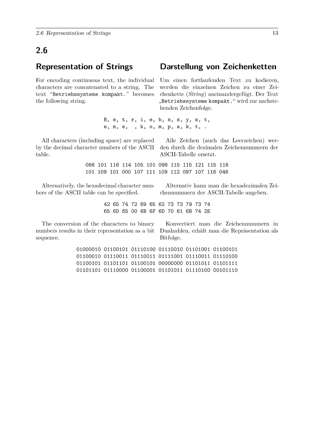
2.6 Representation of Strings . . . .

1
.
.
.
.
.
.
.
.
.
.
.

.
.
.
.
.
.
.
.
.
.
.

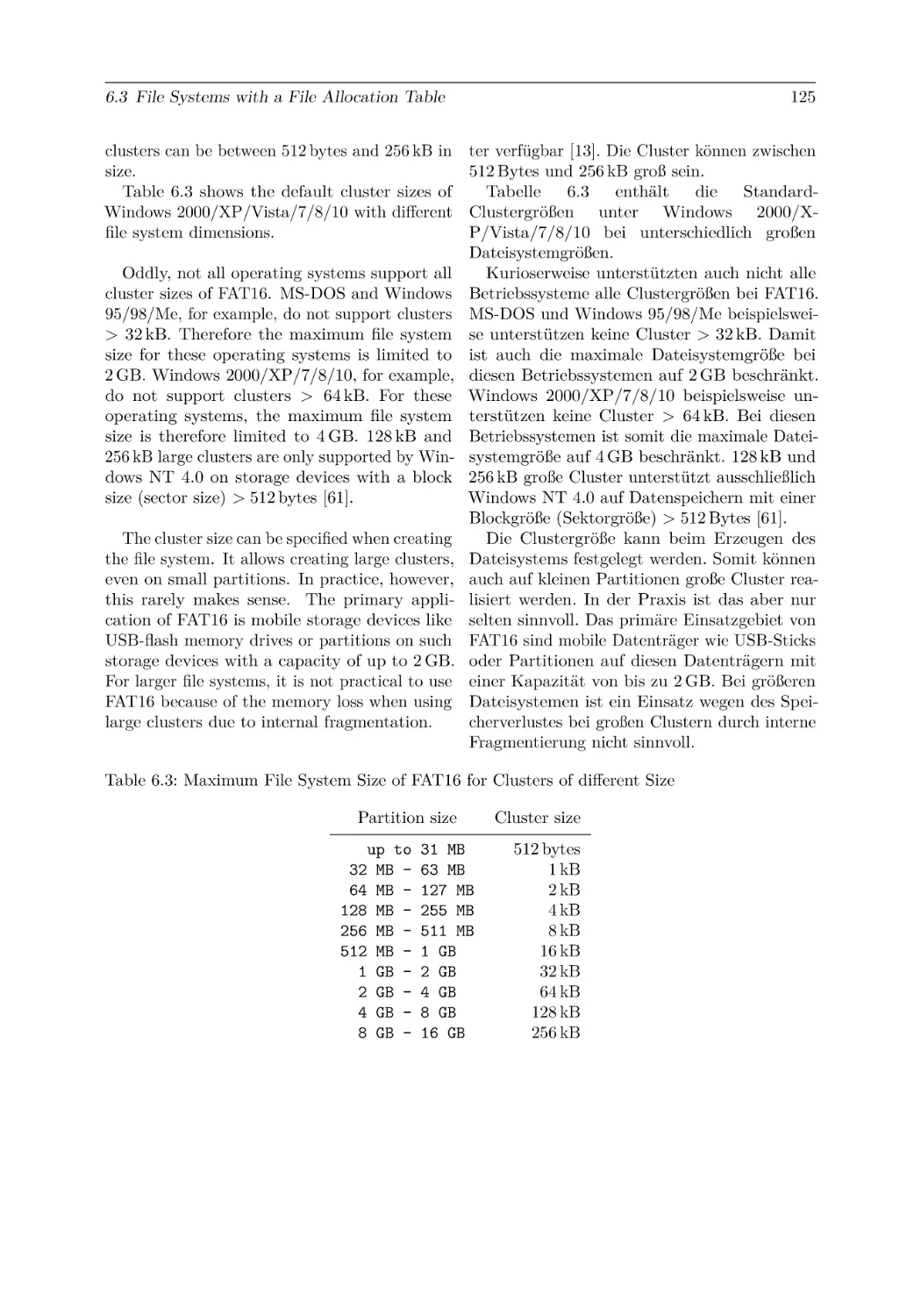
3
3
4
5
5
6
7
8
9
10
12
13

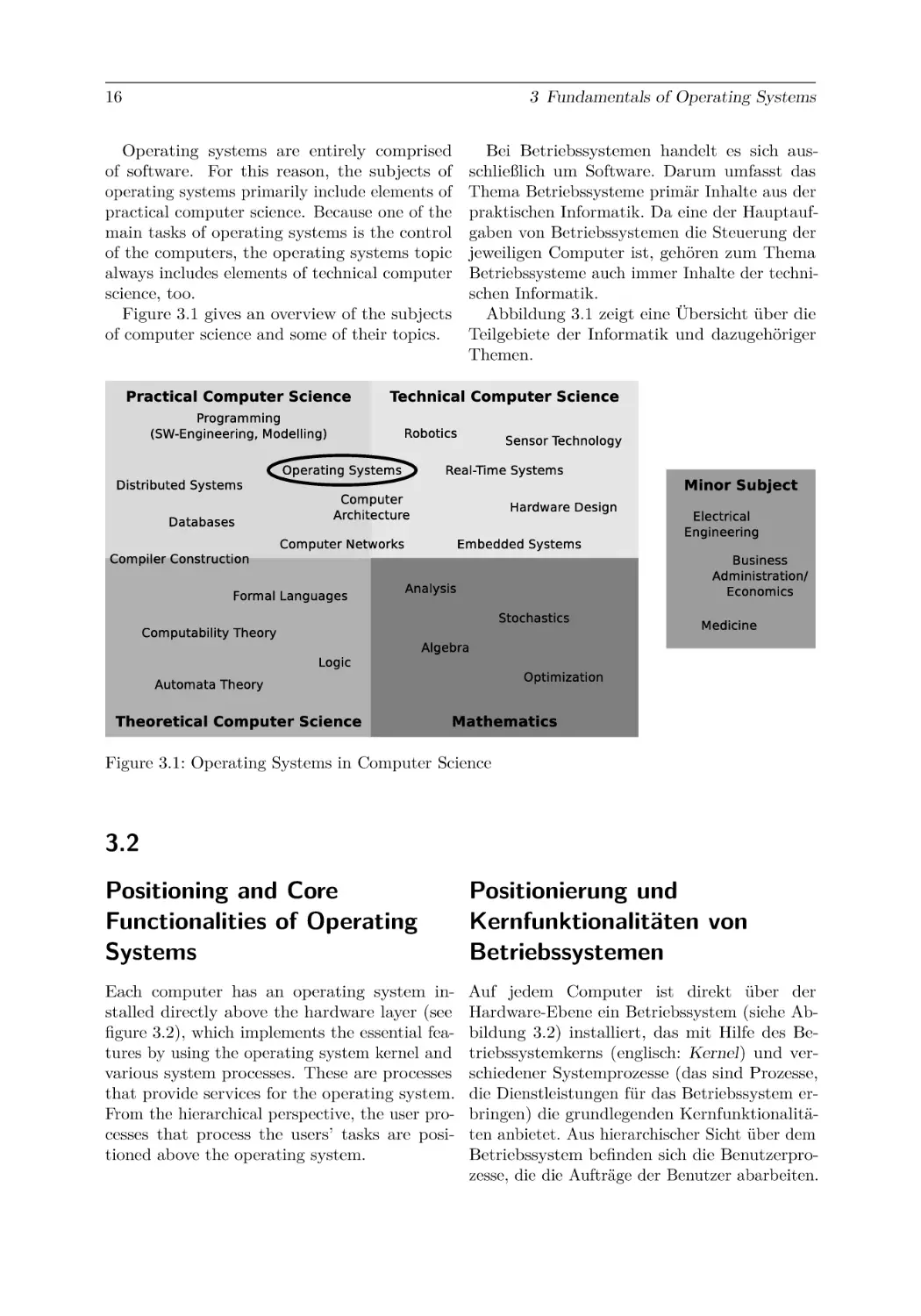
3 Fundamentals of Operating Systems
3.1 Operating Systems in Computer Science . . . . . . . . . . .
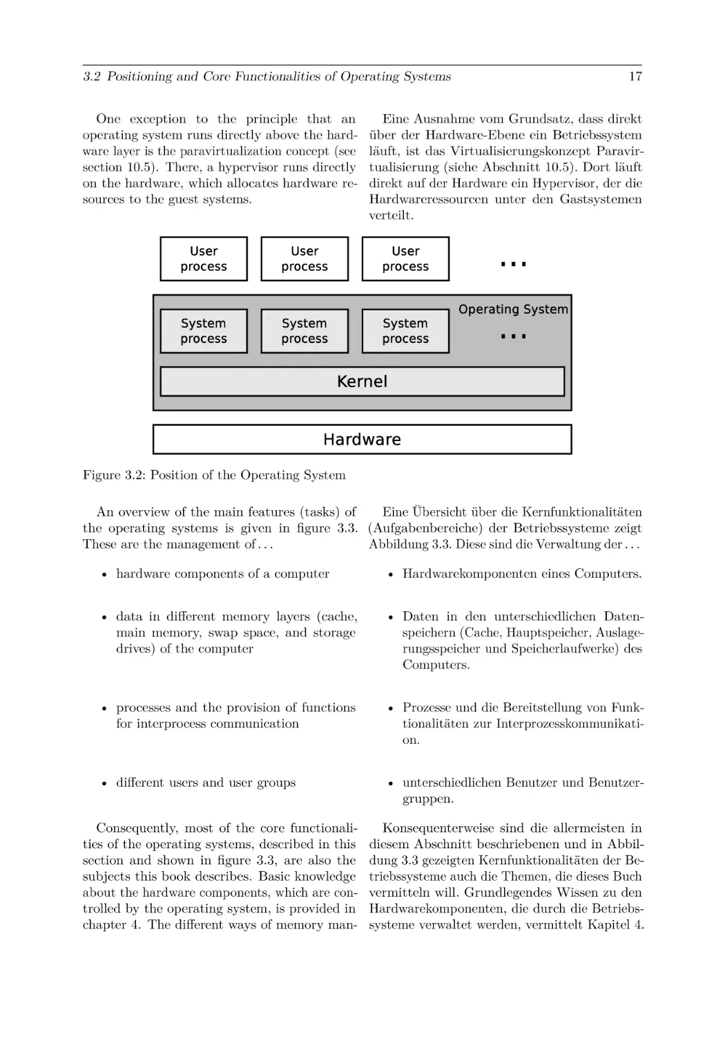
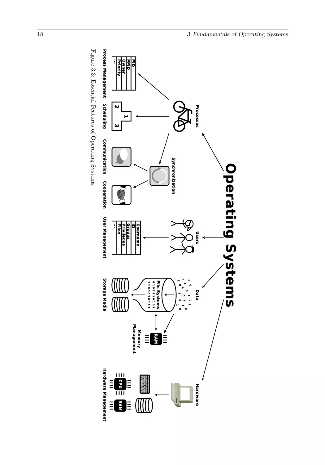
3.2 Positioning and Core Functionalities of Operating Systems
3.3 Evolution of Operating Systems . . . . . . . . . . . . . . . .
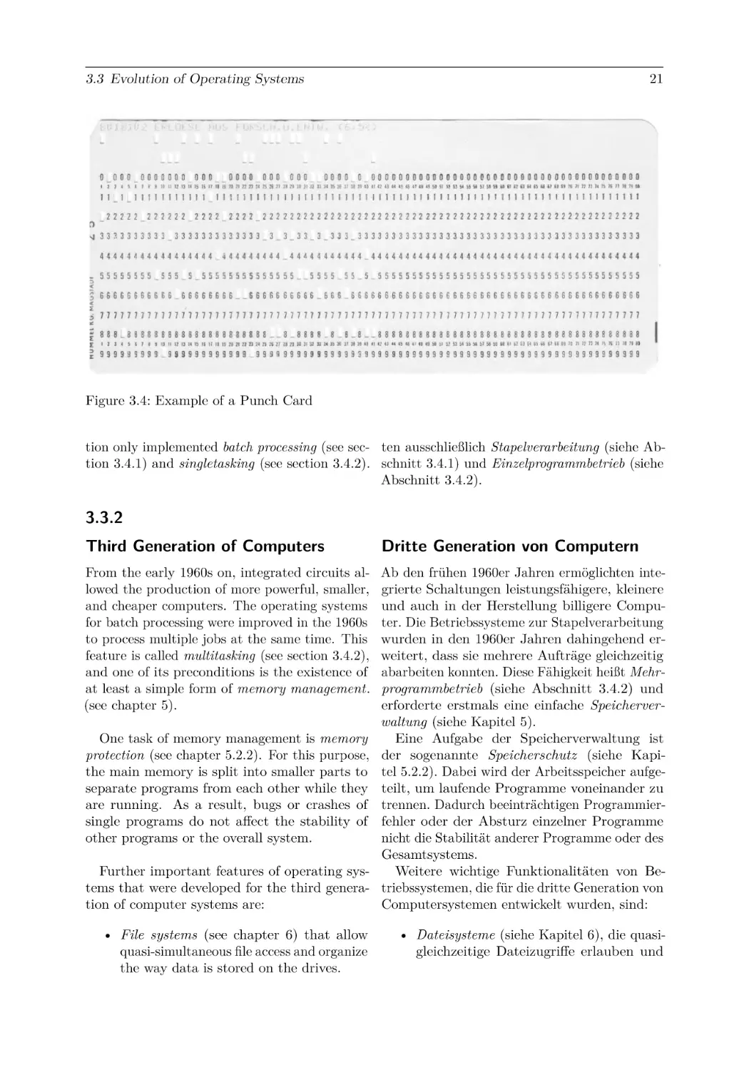
3.3.1 Second Generation of Computers . . . . . . . . . . .
3.3.2 Third Generation of Computers . . . . . . . . . . . .
3.3.3 Fourth Generation of Computers . . . . . . . . . . .
3.4 Operating Modes . . . . . . . . . . . . . . . . . . . . . . . .
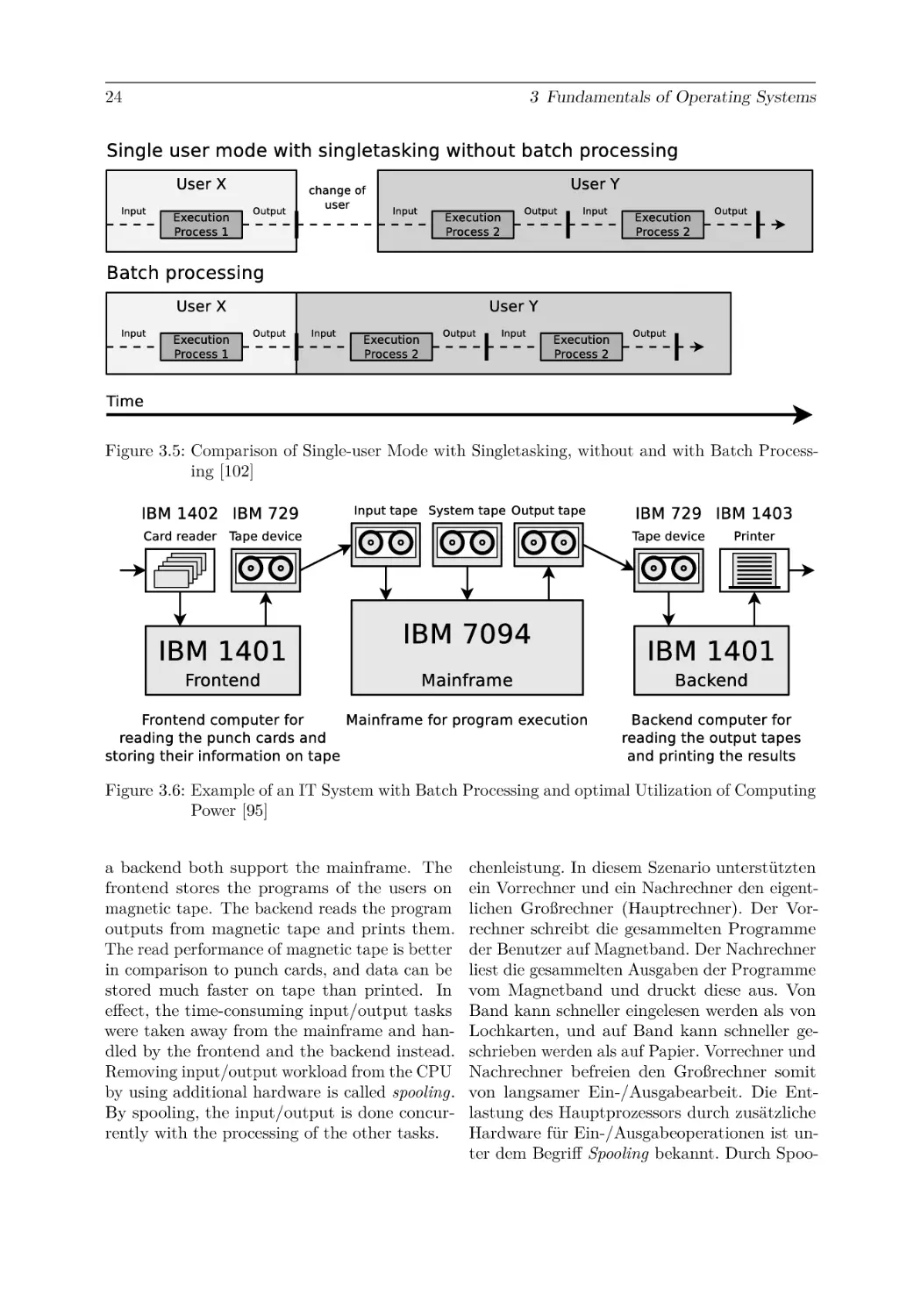
3.4.1 Batch Processing and Time-sharing . . . . . . . . . .
3.4.2 Singletasking and Multitasking . . . . . . . . . . . .
3.4.3 Single-user and Multi-user . . . . . . . . . . . . . . .
3.5 8/16/32/64-Bit Operating Systems . . . . . . . . . . . . . .
3.6 Real-Time Operating Systems . . . . . . . . . . . . . . . . .
3.6.1 Hard and Soft Real-Time Operating Systems . . . .
3.6.2 Architectures of Real-Time Operating Systems . . .
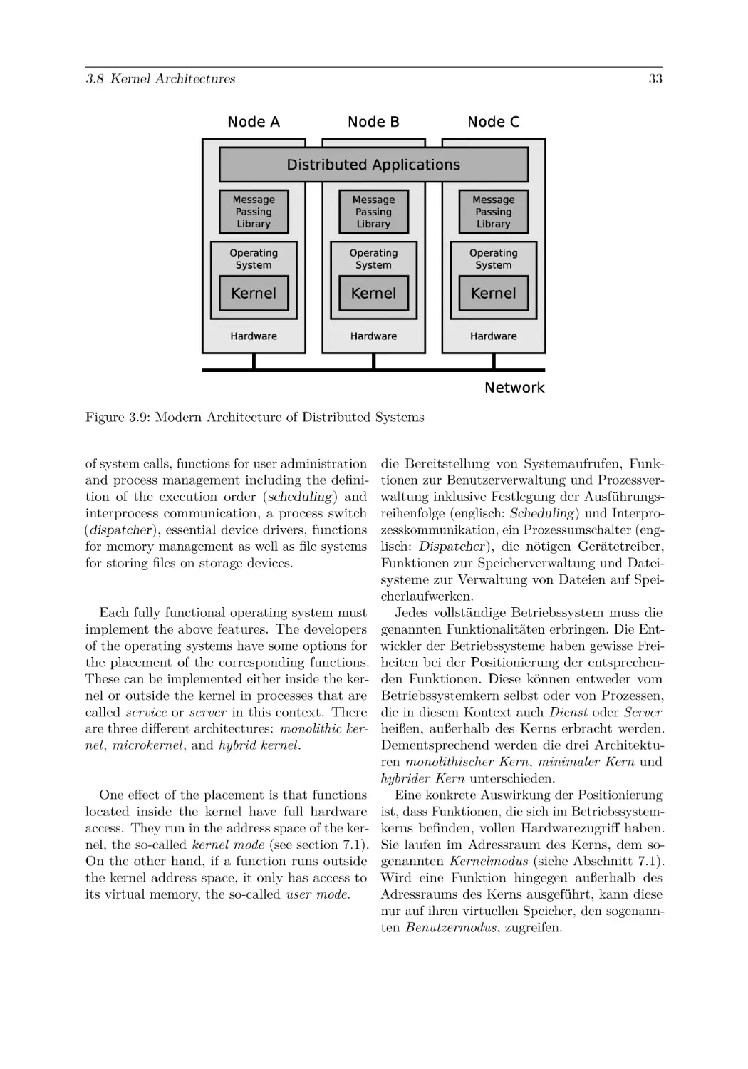
3.7 Distributed Operating Systems . . . . . . . . . . . . . . . .
3.8 Kernel Architectures . . . . . . . . . . . . . . . . . . . . . .
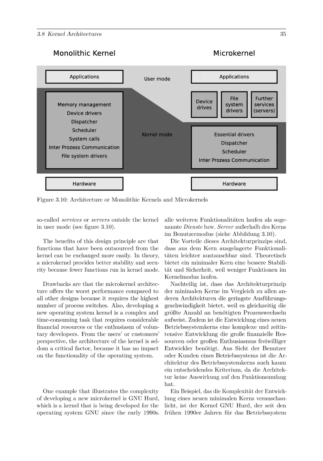
3.8.1 Monolithic Kernels . . . . . . . . . . . . . . . . . . .
3.8.2 Microkernels . . . . . . . . . . . . . . . . . . . . . .
3.8.3 Hybrid Kernels . . . . . . . . . . . . . . . . . . . . .
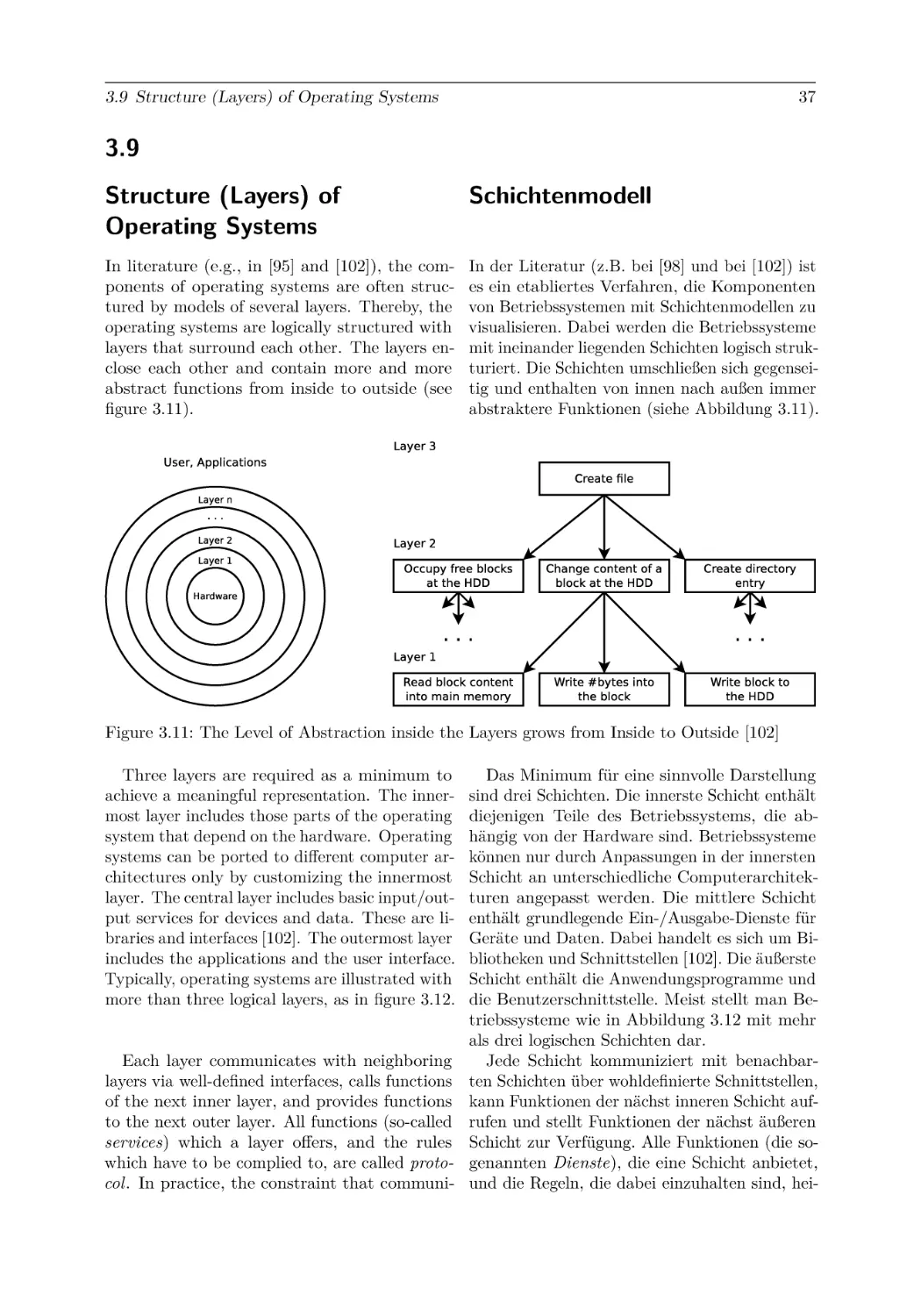
3.9 Structure (Layers) of Operating Systems . . . . . . . . . . .

.
.
.
.
.
.
.
.
.
.
.
.
.
.
.
.
.
.
.
.

15
15
16
19
20
21
22
23
23
25
26
27
28
28
29
30
32
34
34
36
37

4 Fundamentals of Computer Architecture
4.1 Von Neumann Architecture . . . . . . . . . . . . . . . . . . . . . . . . . . . . . . .
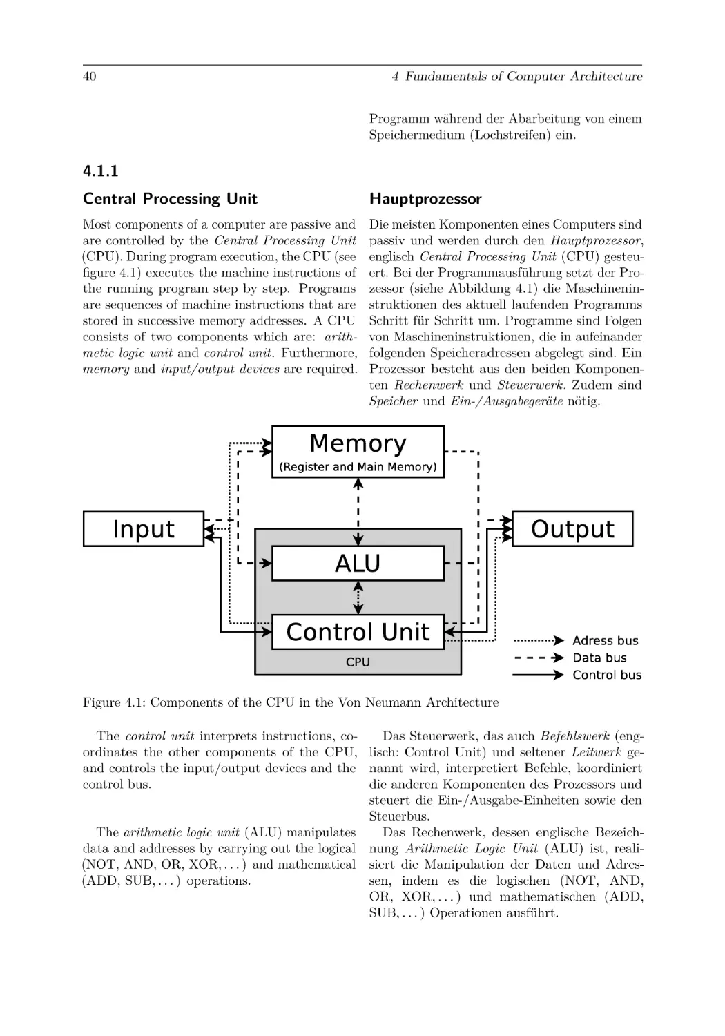
4.1.1 Central Processing Unit . . . . . . . . . . . . . . . . . . . . . . . . . . . . .
4.1.2 Fetch-Decode-Execute Cycle . . . . . . . . . . . . . . . . . . . . . . . . . . .

39
39
40
41

.
.
.
.
.
.
.
.
.
.
.

Contents
4.1.3 Bus Lines . . . . . . . . . . . . . . . . .
4.2 Input/Output Devices . . . . . . . . . . . . . .
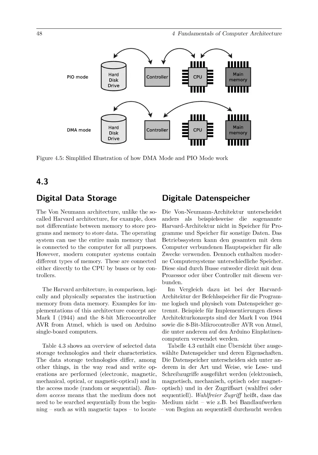
4.3 Digital Data Storage . . . . . . . . . . . . . . .
4.4 Memory Hierarchy . . . . . . . . . . . . . . . .
4.4.1 Register . . . . . . . . . . . . . . . . . .
4.4.2 Cache . . . . . . . . . . . . . . . . . . .
4.4.3 Cache Write Policies . . . . . . . . . . .
4.4.4 Main Memory . . . . . . . . . . . . . . .
4.4.5 Hard Disk Drives . . . . . . . . . . . . .
4.4.6 Addressing Data on Hard Disk Drives .
4.4.7 Access Time of HDDs . . . . . . . . . .
4.4.8 Solid-State Drives . . . . . . . . . . . .
4.4.9 Reading Data from Flash Memory Cells
4.5 RAID . . . . . . . . . . . . . . . . . . . . . . .
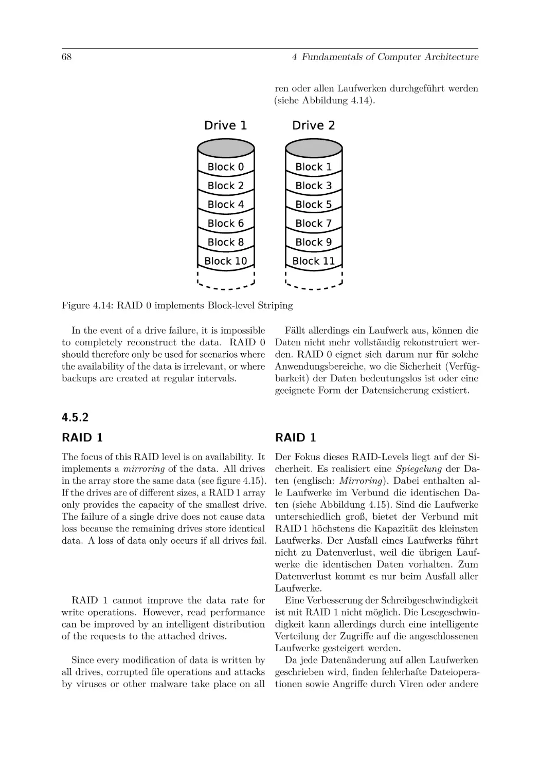
4.5.1 RAID 0 . . . . . . . . . . . . . . . . . .
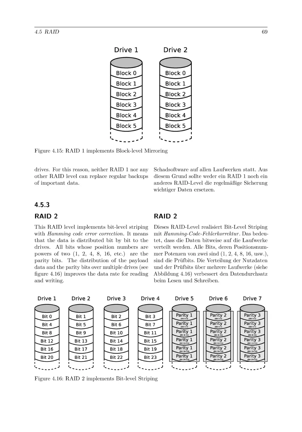
4.5.2 RAID 1 . . . . . . . . . . . . . . . . . .
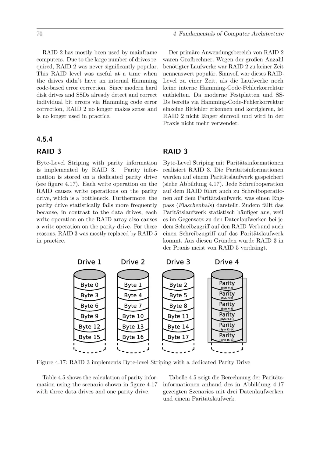
4.5.3 RAID 2 . . . . . . . . . . . . . . . . . .
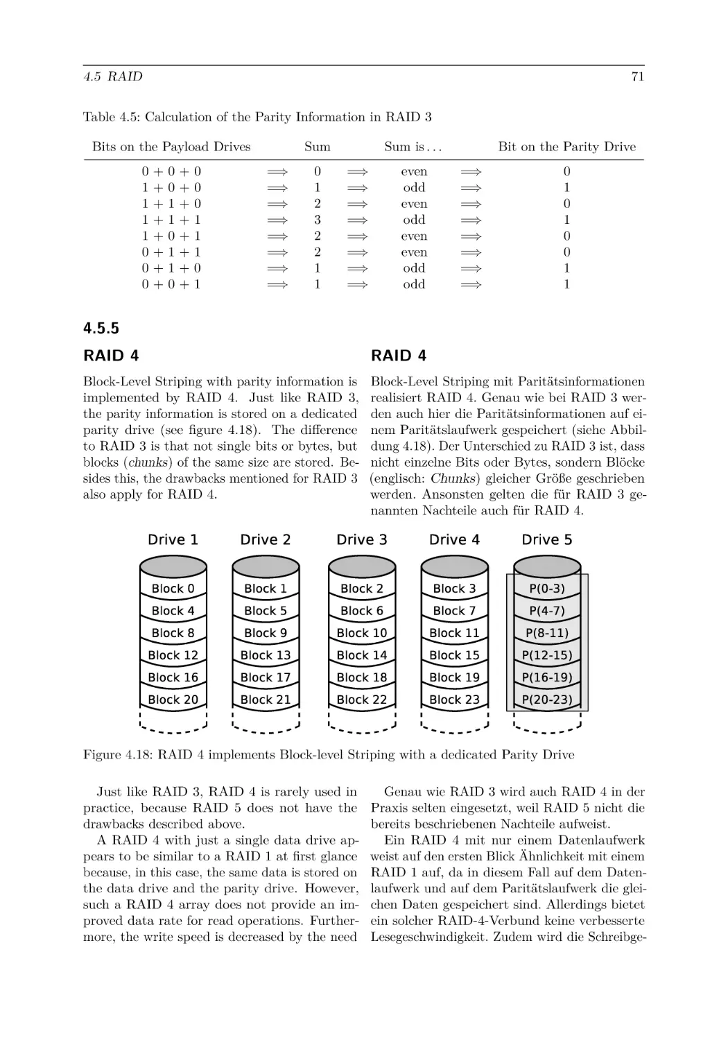
4.5.4 RAID 3 . . . . . . . . . . . . . . . . . .
4.5.5 RAID 4 . . . . . . . . . . . . . . . . . .
4.5.6 RAID 5 . . . . . . . . . . . . . . . . . .
4.5.7 RAID 6 . . . . . . . . . . . . . . . . . .
4.5.8 RAID Combinations . . . . . . . . . . .

.
.
.
.
.
.
.
.
.
.
.
.
.
.
.
.
.
.
.
.
.
.

42
45
48
49
52
52
53
54
55
56
58
58
60
64
67
68
69
70
71
72
73
73

5 Memory Management
5.1 Memory Management Concepts . . . . . . . . . . . . . . . . .
5.1.1 Static Partitioning . . . . . . . . . . . . . . . . . . . .
5.1.2 Dynamic Partitioning . . . . . . . . . . . . . . . . . .
5.1.3 Buddy Memory Allocation . . . . . . . . . . . . . . . .
5.2 Memory Addressing in Practice . . . . . . . . . . . . . . . . .
5.2.1 Real Mode . . . . . . . . . . . . . . . . . . . . . . . .
5.2.2 Protected Mode and Virtual Memory . . . . . . . . .
5.2.3 Page-based Memory Management (Paging) . . . . . .
5.2.4 Segment-based Memory Management (Segmentation)
5.2.5 State of the Art of Virtual Memory . . . . . . . . . . .
5.2.6 Kernel Space and User Space . . . . . . . . . . . . . .
5.3 Page Replacement Strategies . . . . . . . . . . . . . . . . . .
5.3.1 Optimal Strategy . . . . . . . . . . . . . . . . . . . . .
5.3.2 Least Recently Used . . . . . . . . . . . . . . . . . . .
5.3.3 Least Frequently Used . . . . . . . . . . . . . . . . . .
5.3.4 First In First Out . . . . . . . . . . . . . . . . . . . .
5.3.5 Clock / Second Chance . . . . . . . . . . . . . . . . .
5.3.6 Random . . . . . . . . . . . . . . . . . . . . . . . . . .

.
.
.
.
.
.
.
.
.
.
.
.
.
.
.
.
.
.

75
75
76
77
79
83
84
88
90
99
100
102
103
104
105
106
107
108
109

6 File Systems
6.1 Technical Principles of File Systems . . .
6.2 Block Addressing in Linux File Systems .
6.2.1 Minix . . . . . . . . . . . . . . . .
6.2.2 ext2/3/4 . . . . . . . . . . . . . . .
6.3 File Systems with a File Allocation Table
6.3.1 FAT12 . . . . . . . . . . . . . . . .
6.3.2 FAT16 . . . . . . . . . . . . . . . .
6.3.3 FAT32 . . . . . . . . . . . . . . . .

.
.
.
.
.
.
.
.

111
111
112
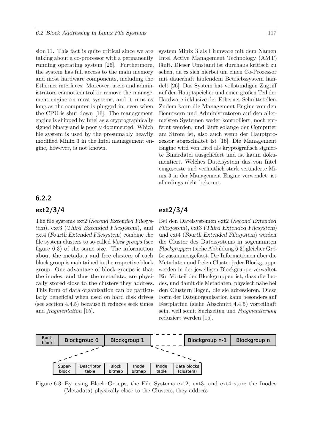
115
117
120
124
124
126

.
.
.
.
.
.
.
.

.
.
.
.
.
.
.
.
.
.
.
.
.
.
.
.
.
.
.
.
.
.

.
.
.
.
.
.
.
.

.
.
.
.
.
.
.
.
.
.
.
.
.
.
.
.
.
.
.
.
.
.

.
.
.
.
.
.
.
.

.
.
.
.
.
.
.
.
.
.
.
.
.
.
.
.
.
.
.
.
.
.

.
.
.
.
.
.
.
.

.
.
.
.
.
.
.
.
.
.
.
.
.
.
.
.
.
.
.
.
.
.

.
.
.
.
.
.
.
.

.
.
.
.
.
.
.
.
.
.
.
.
.
.
.
.
.
.
.
.
.
.

.
.
.
.
.
.
.
.

.
.
.
.
.
.
.
.
.
.
.
.
.
.
.
.
.
.
.
.
.
.

.
.
.
.
.
.
.
.

.
.
.
.
.
.
.
.
.
.
.
.
.
.
.
.
.
.
.
.
.
.

.
.
.
.
.
.
.
.

Contents
6.3.4 VFAT . . . . . . . . . . . . . . .
6.3.5 exFAT . . . . . . . . . . . . . . .
6.4 Journaling File Systems . . . . . . . . .
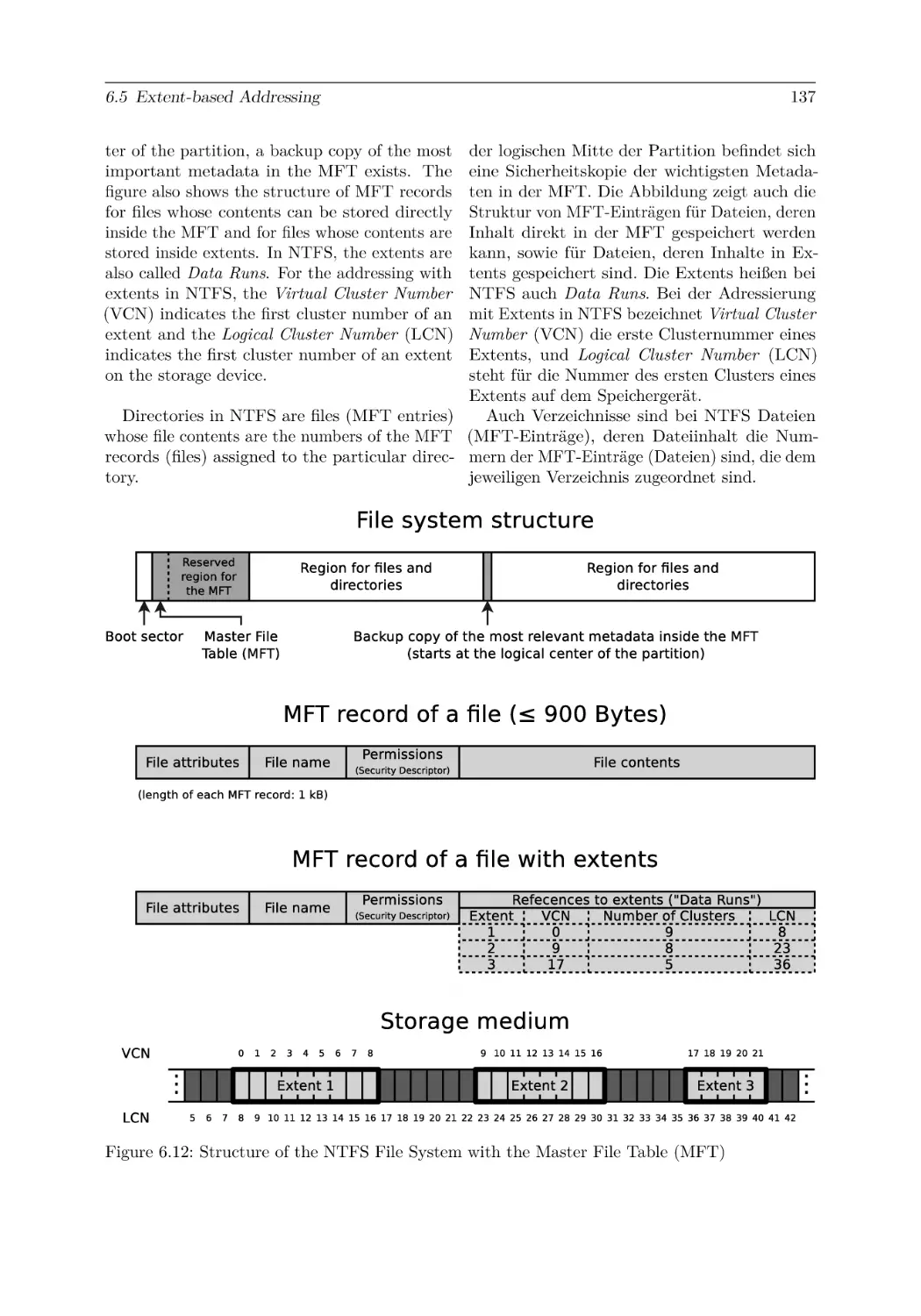
6.5 Extent-based Addressing . . . . . . . . .
6.5.1 ext4 . . . . . . . . . . . . . . . .
6.5.2 NTFS . . . . . . . . . . . . . . .
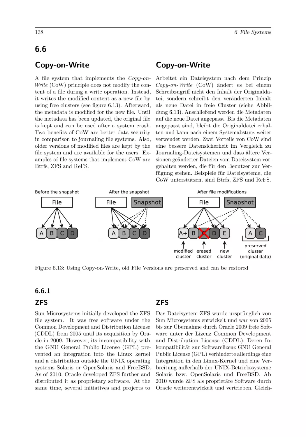
6.6 Copy-on-Write . . . . . . . . . . . . . .
6.6.1 ZFS . . . . . . . . . . . . . . . .
6.6.2 Btrfs . . . . . . . . . . . . . . . .
6.6.3 ReFS . . . . . . . . . . . . . . .
6.7 Accelerating Data Access with a Cache .
6.8 Defragmentation . . . . . . . . . . . . .

xi
.
.
.
.
.
.
.
.
.
.
.
.

.
.
.
.
.
.
.
.
.
.
.
.

126
127
130
131
133
135
138
138
140
140
141
142

7 System Calls
7.1 User Mode and Kernel Mode . . . . . . . . . . . . . . . . . . . . . . . . . . . . . .
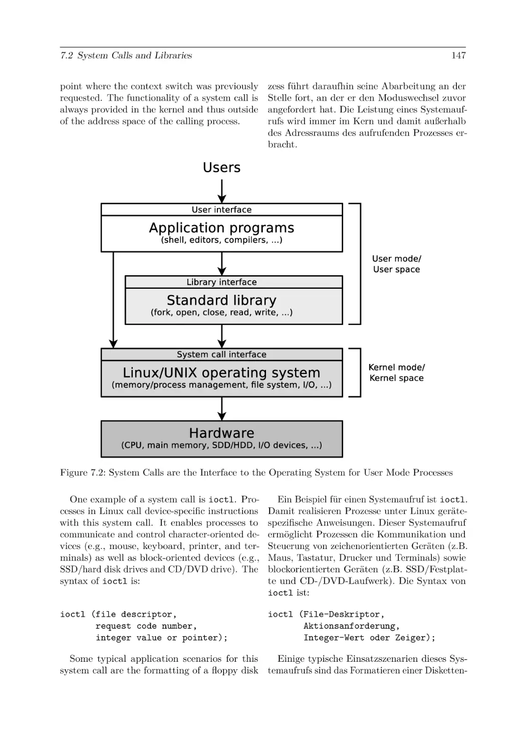
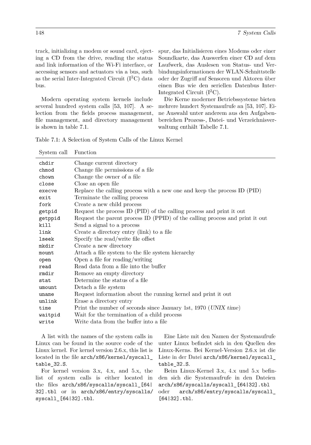
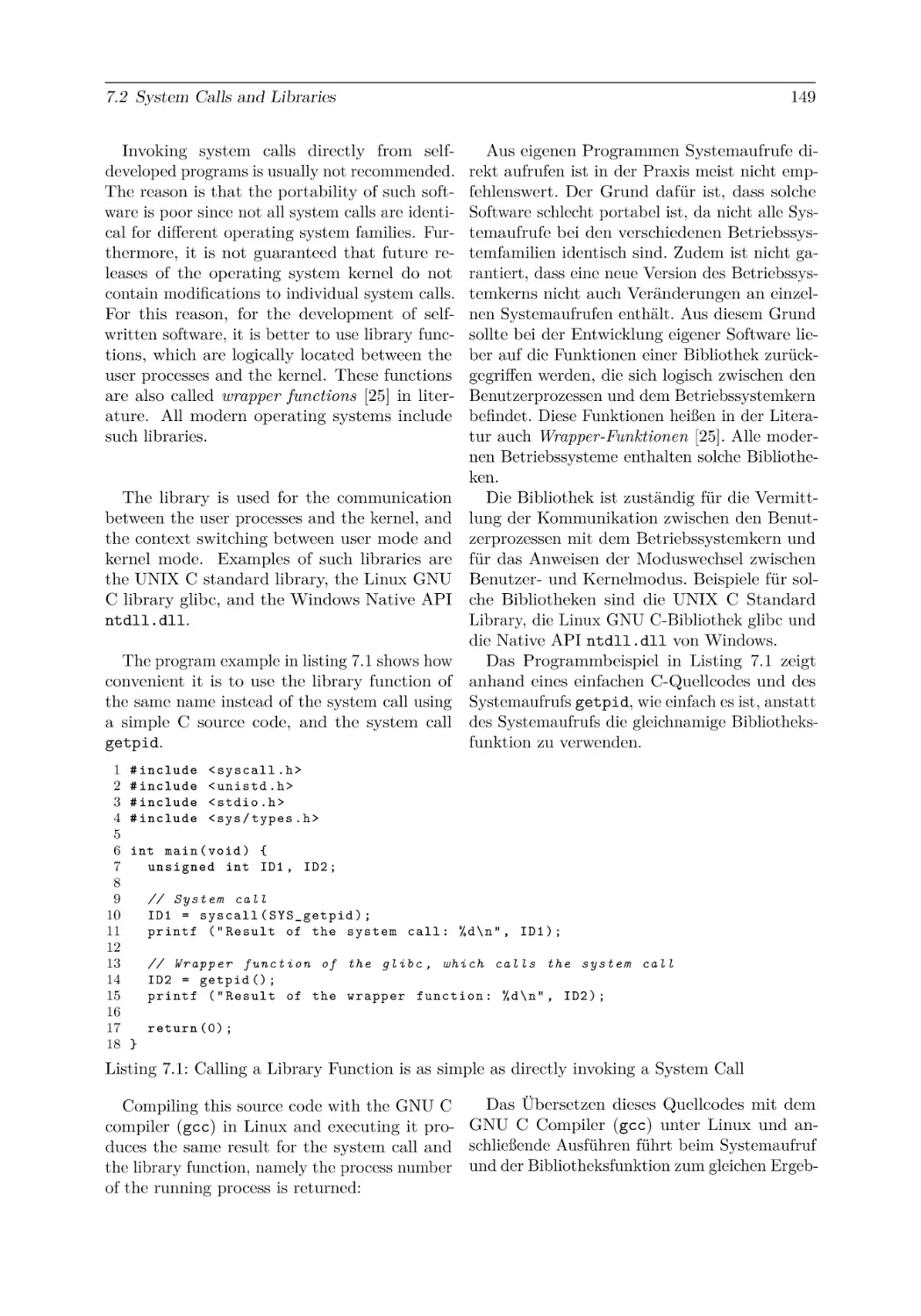
7.2 System Calls and Libraries . . . . . . . . . . . . . . . . . . . . . . . . . . . . . . .
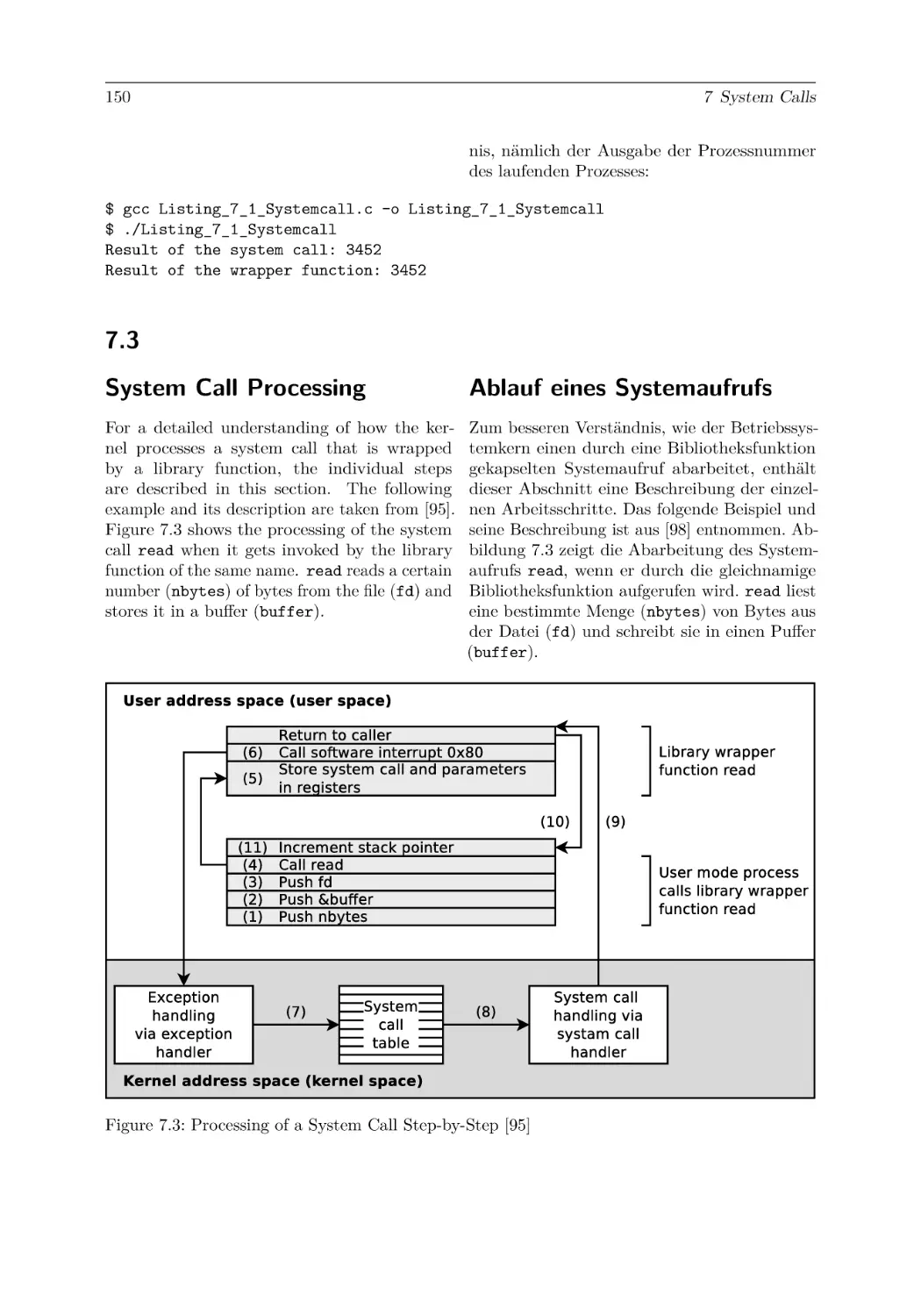
7.3 System Call Processing . . . . . . . . . . . . . . . . . . . . . . . . . . . . . . . . .

145
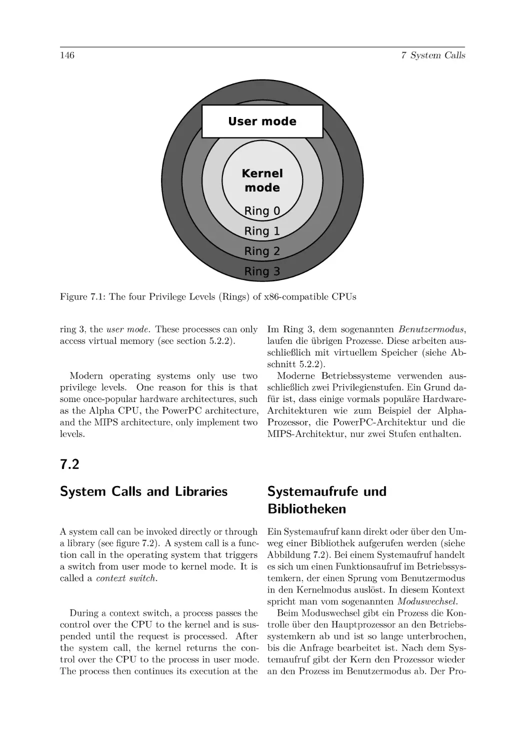
145
146
150

8 Process Management
8.1 Process Context . . . . . . . . . . . . . . . . . . .
8.2 Process States . . . . . . . . . . . . . . . . . . . .
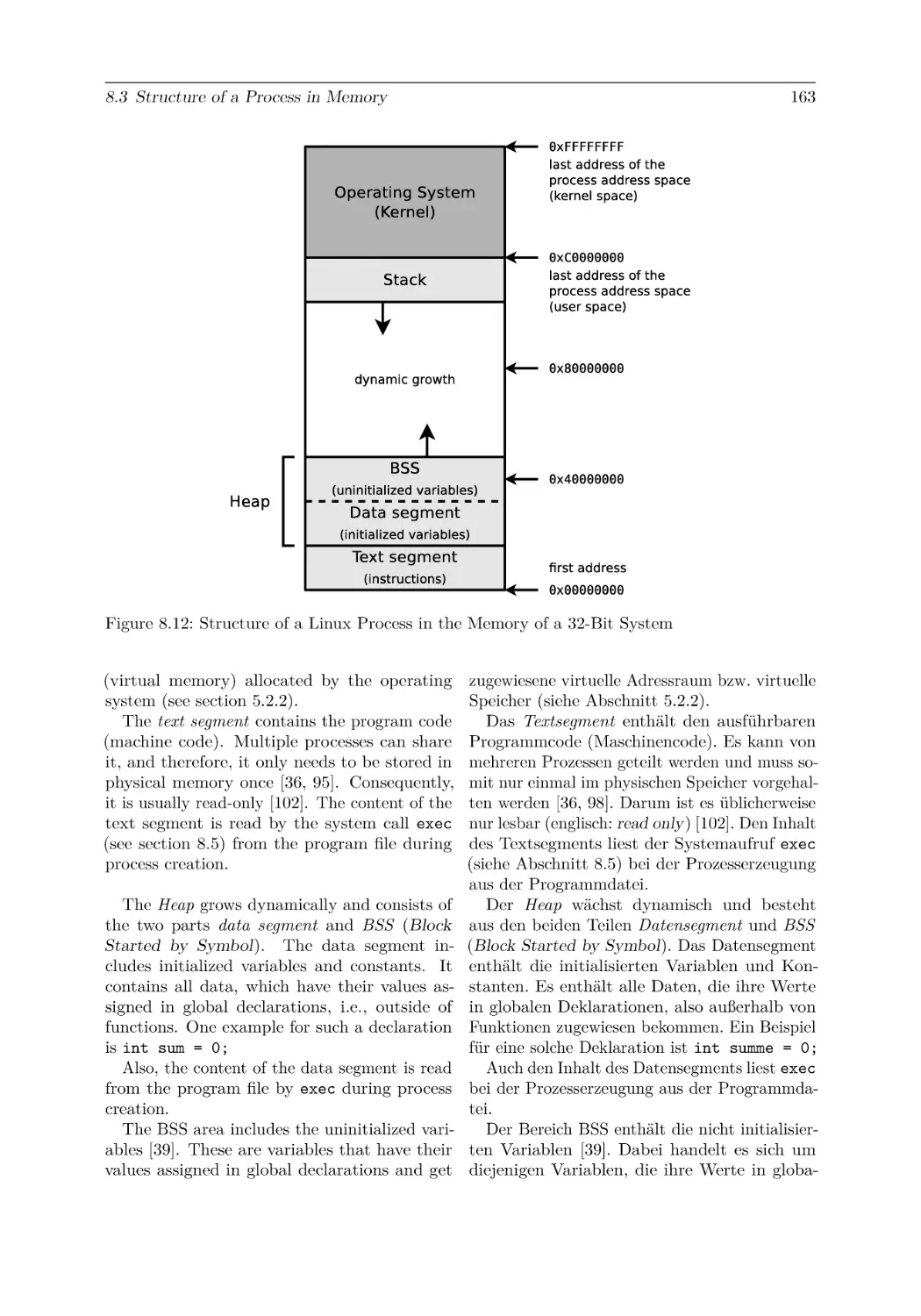
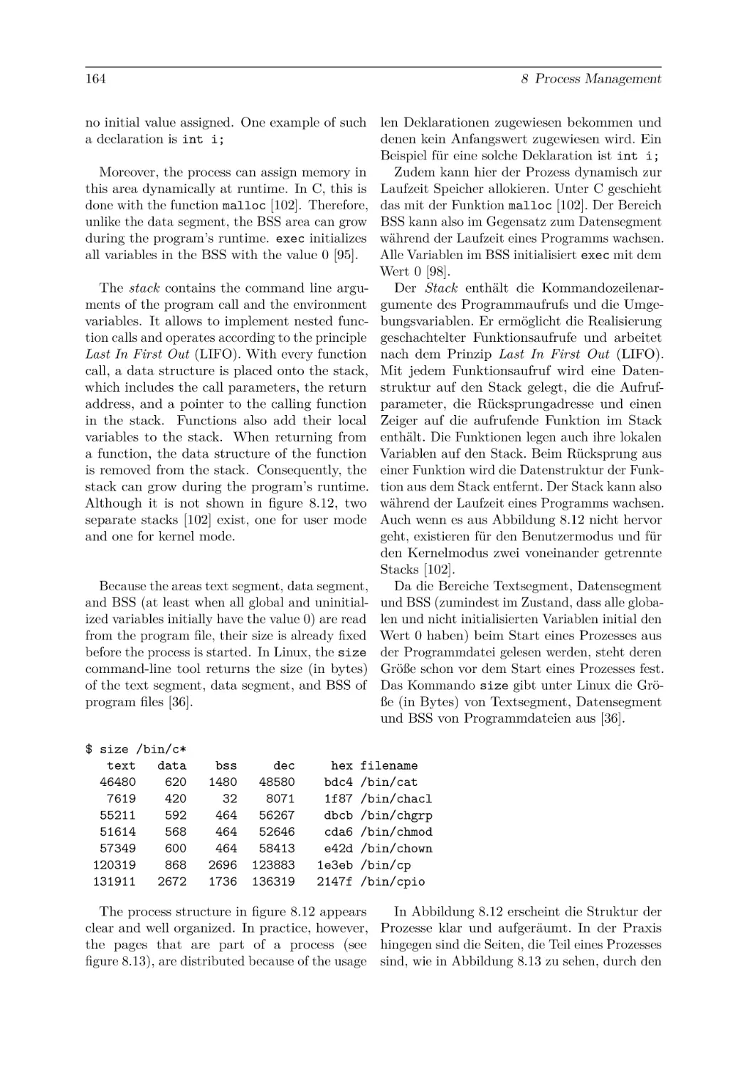
8.3 Structure of a Process in Memory . . . . . . . . .
8.4 Process Creation via fork . . . . . . . . . . . . . .
8.5 Replacing Processes via exec . . . . . . . . . . . .
8.6 Process Switching and Process Scheduling . . . . .
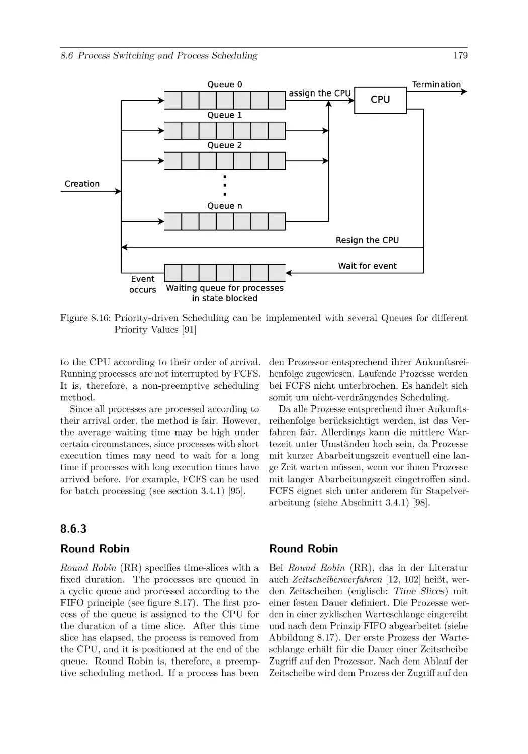
8.6.1 Priority-driven Scheduling . . . . . . . . . .
8.6.2 First Come First Served . . . . . . . . . . .
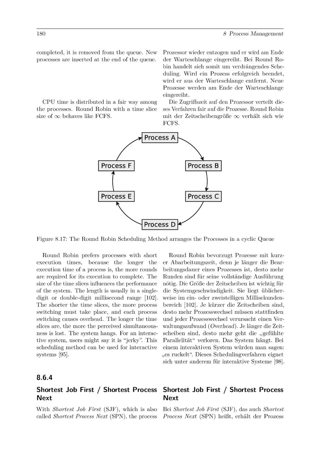
8.6.3 Round Robin . . . . . . . . . . . . . . . . .
8.6.4 Shortest Job First / Shortest Process Next
8.6.5 Shortest Remaining Time First . . . . . . .
8.6.6 Longest Job First . . . . . . . . . . . . . . .
8.6.7 Longest Remaining Time First . . . . . . .
8.6.8 Highest Response Ratio Next . . . . . . . .
8.6.9 Earliest Deadline First . . . . . . . . . . . .
8.6.10 Fair-Share Scheduling . . . . . . . . . . . .
8.6.11 Multilevel Scheduling . . . . . . . . . . . .
8.6.12 Scheduling of Linux Operating Systems . .

.
.
.
.
.
.
.
.
.
.
.
.
.
.
.
.
.
.

153
153
155
162
165
171
175
177
178
179
180
181
182
182
183
183
184
185
187

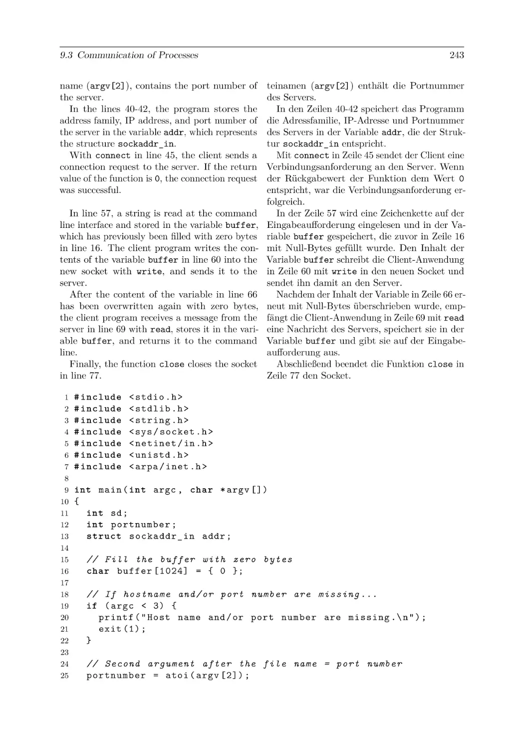
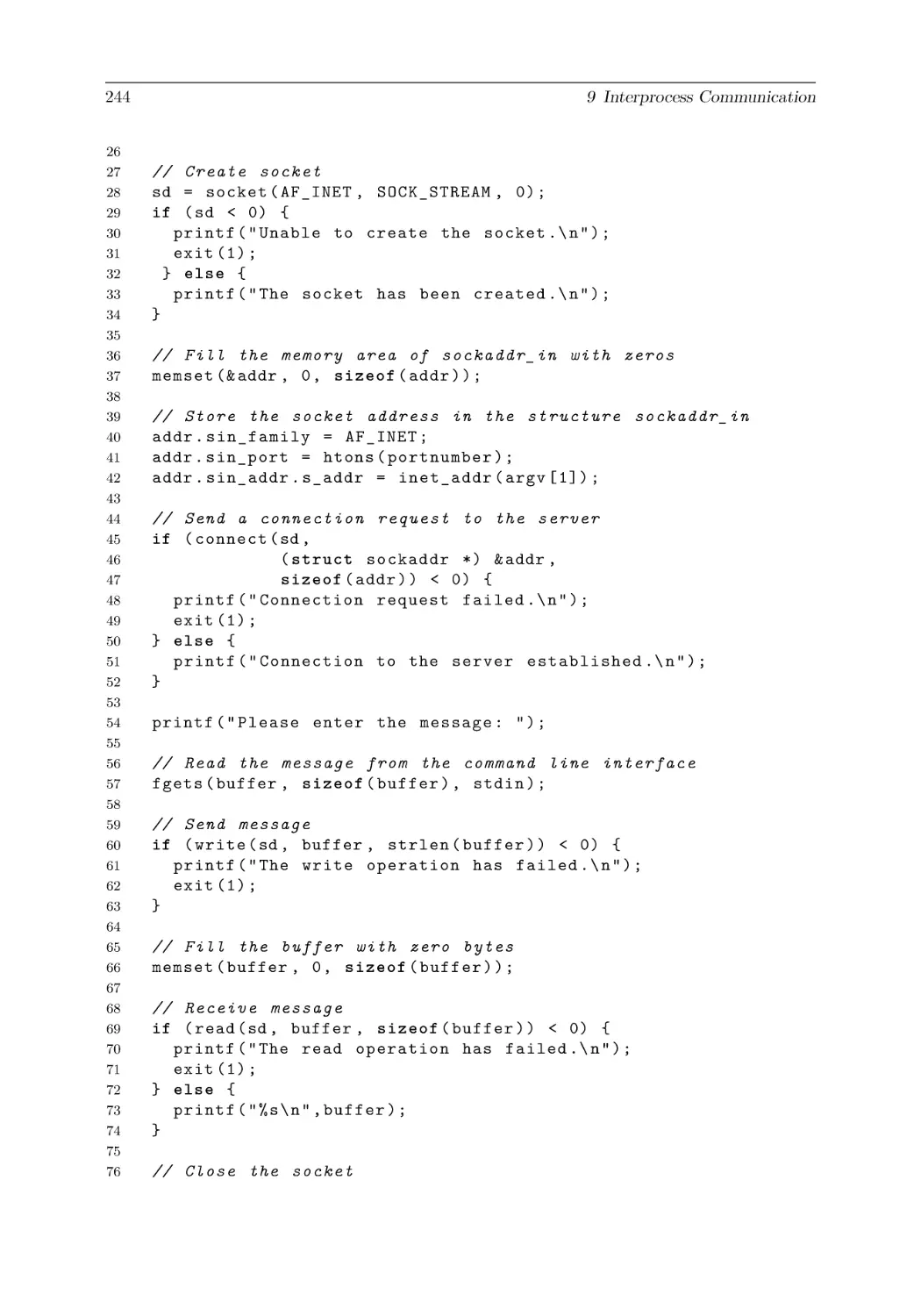
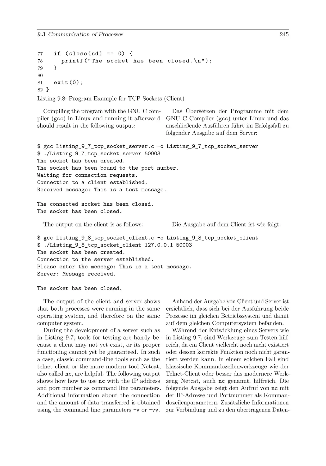
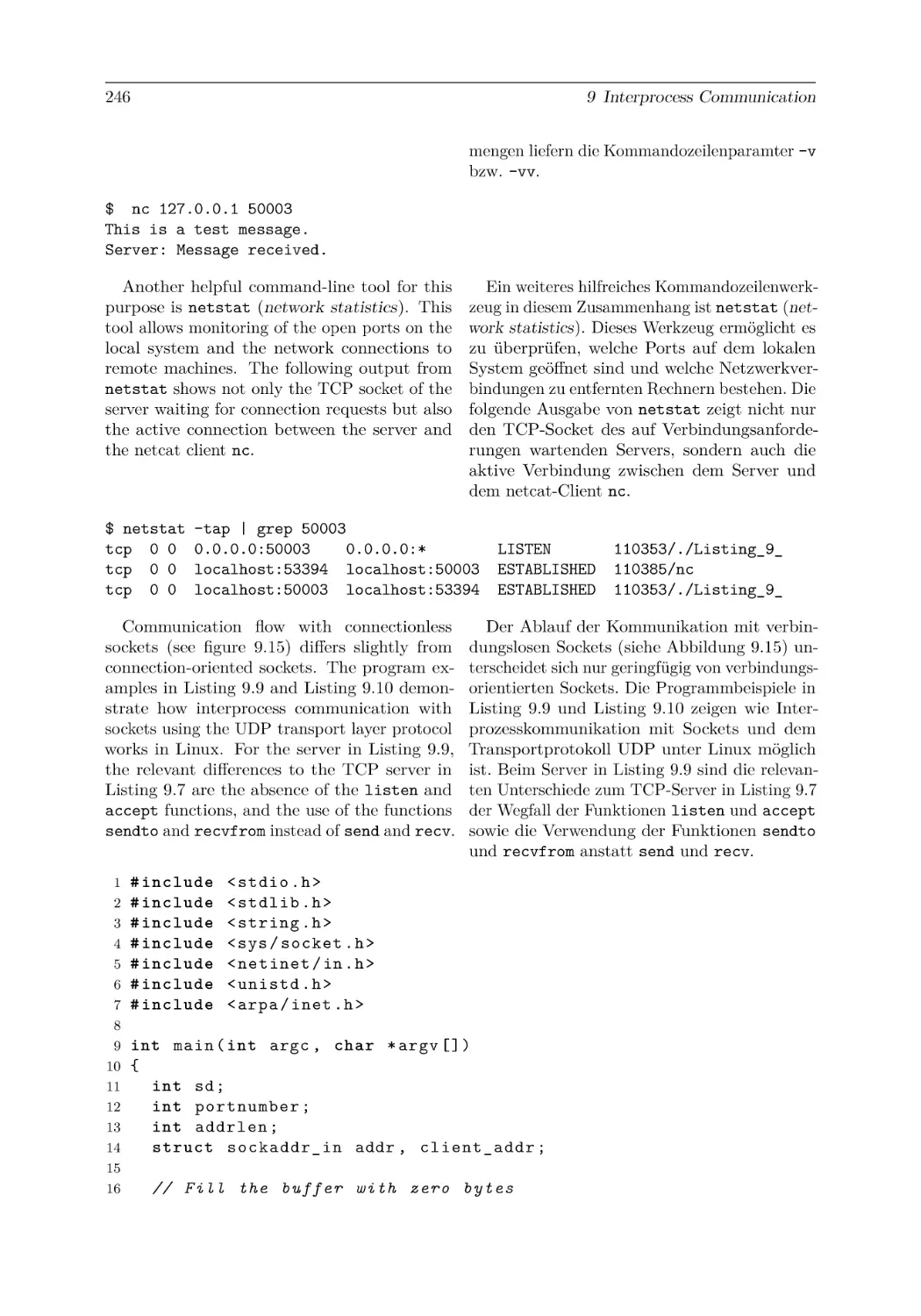
9 Interprocess Communication
9.1 Critical Sections and Race Conditions . . . . . . . . . .
9.2 Synchronization of Processes . . . . . . . . . . . . . . .
9.2.1 Speciﬁcation of the Execution Order of Processes
9.2.2 Protecting Critical Sections by Blocking . . . . .
9.2.3 Starvation and Deadlock . . . . . . . . . . . . . .
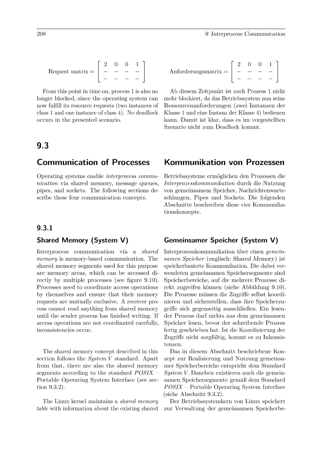
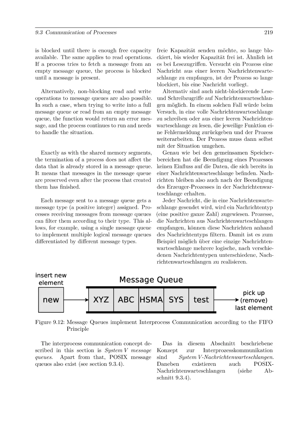
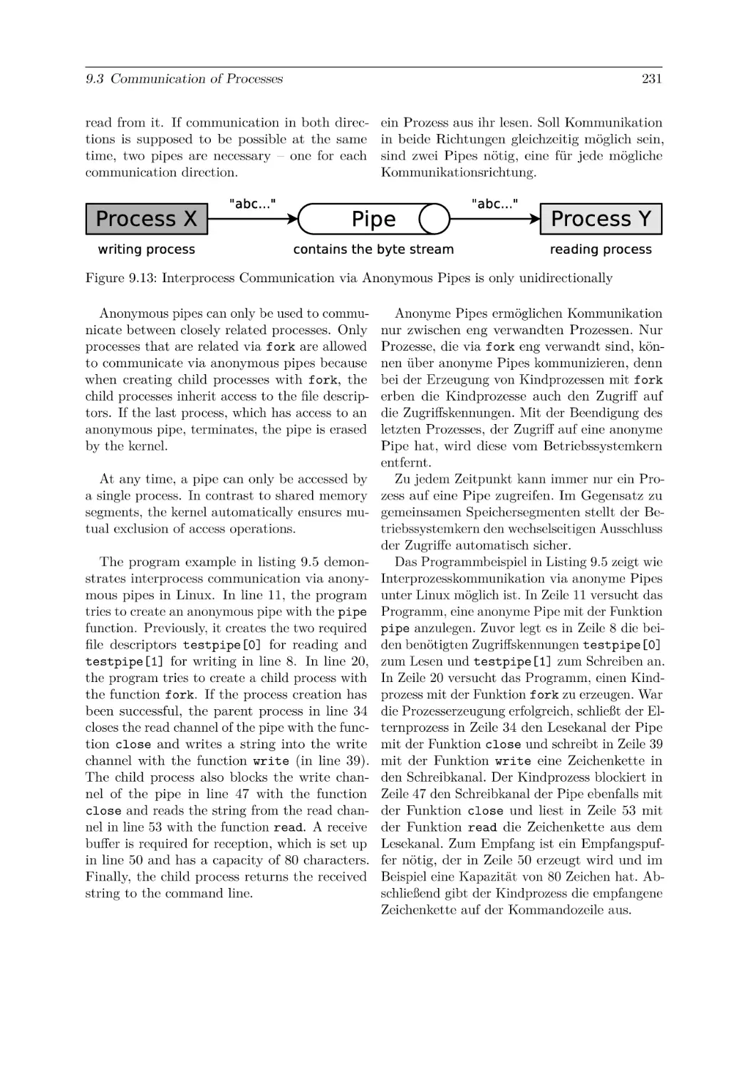
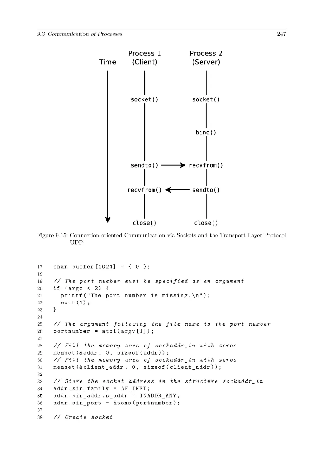
9.3 Communication of Processes . . . . . . . . . . . . . . .
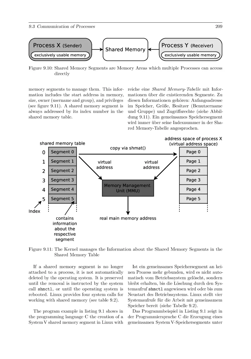
9.3.1 Shared Memory (System V) . . . . . . . . . . . .
9.3.2 Shared Memory (POSIX) . . . . . . . . . . . . .
9.3.3 Message Queues (System V) . . . . . . . . . . . .
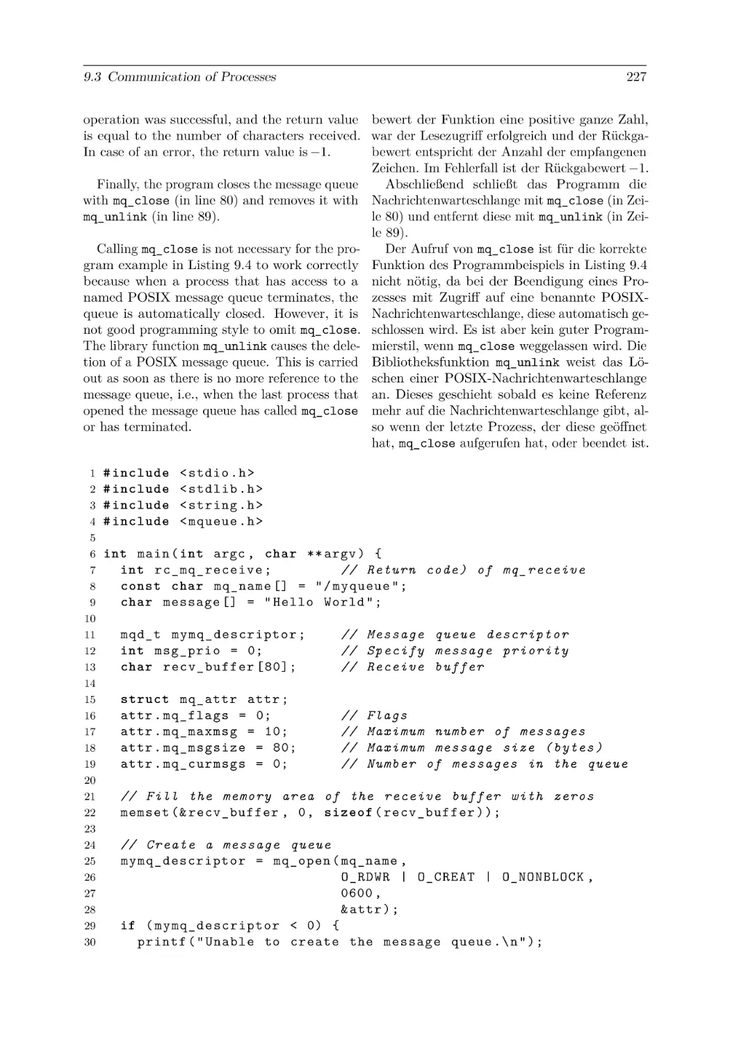
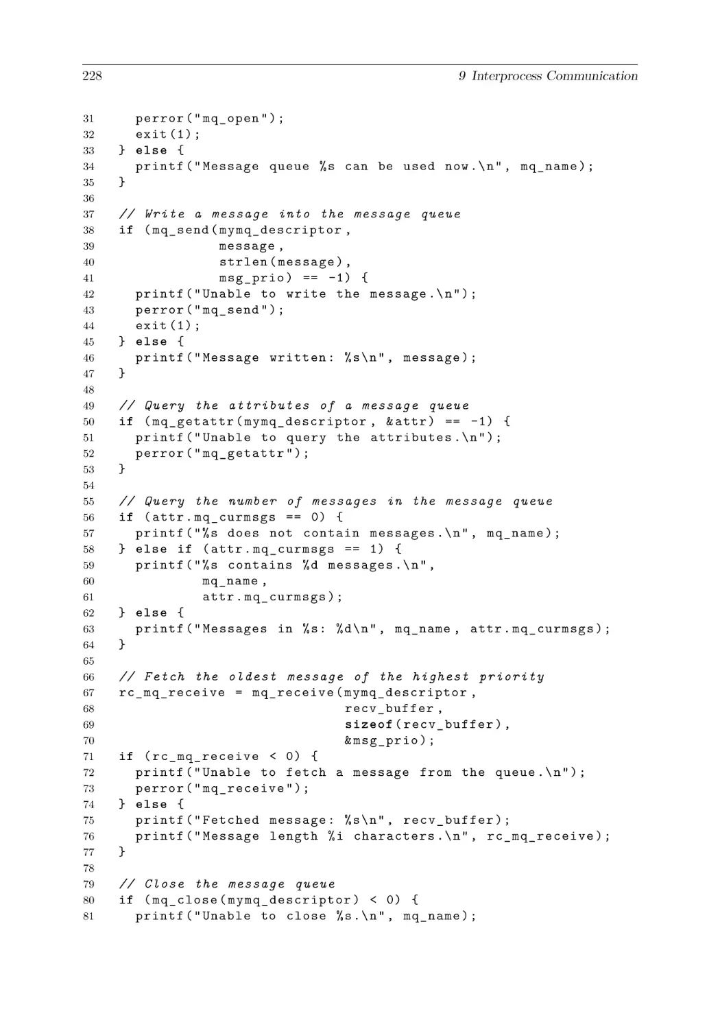
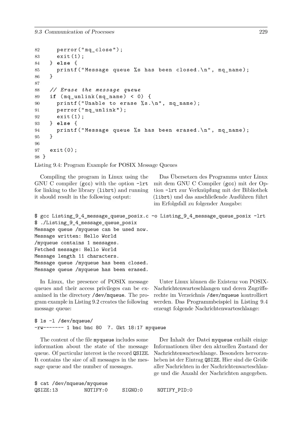
9.3.4 Message Queues (POSIX) . . . . . . . . . . . . .
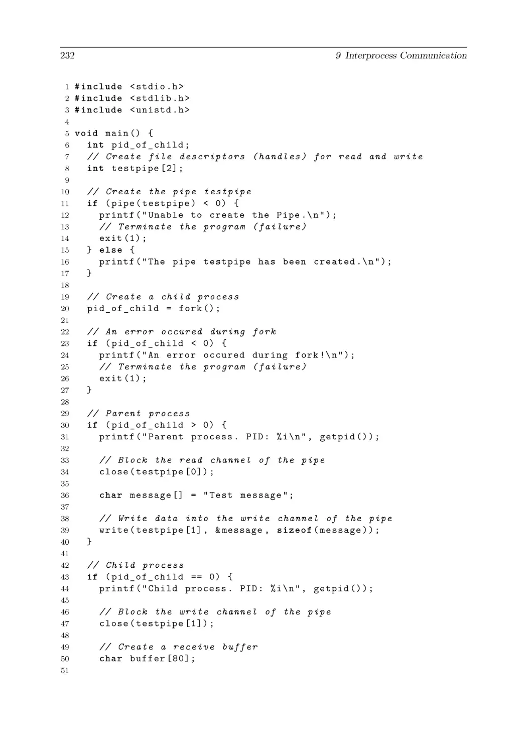
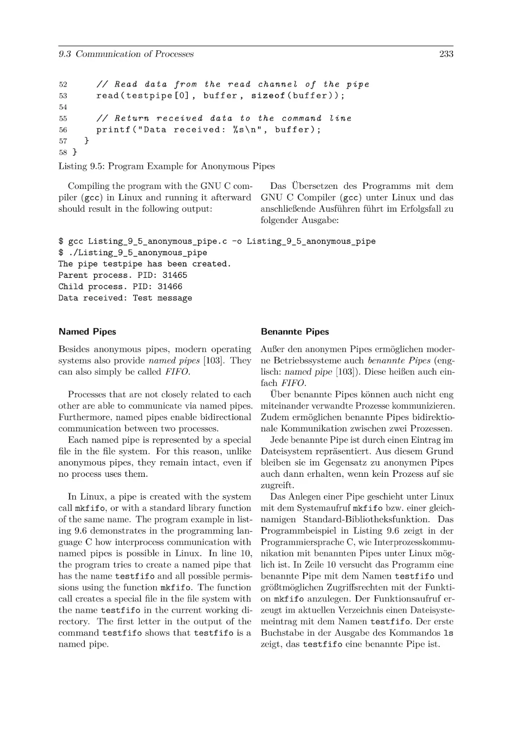
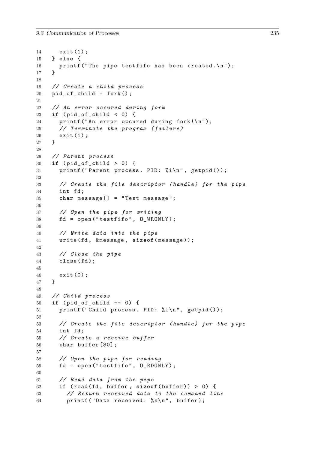
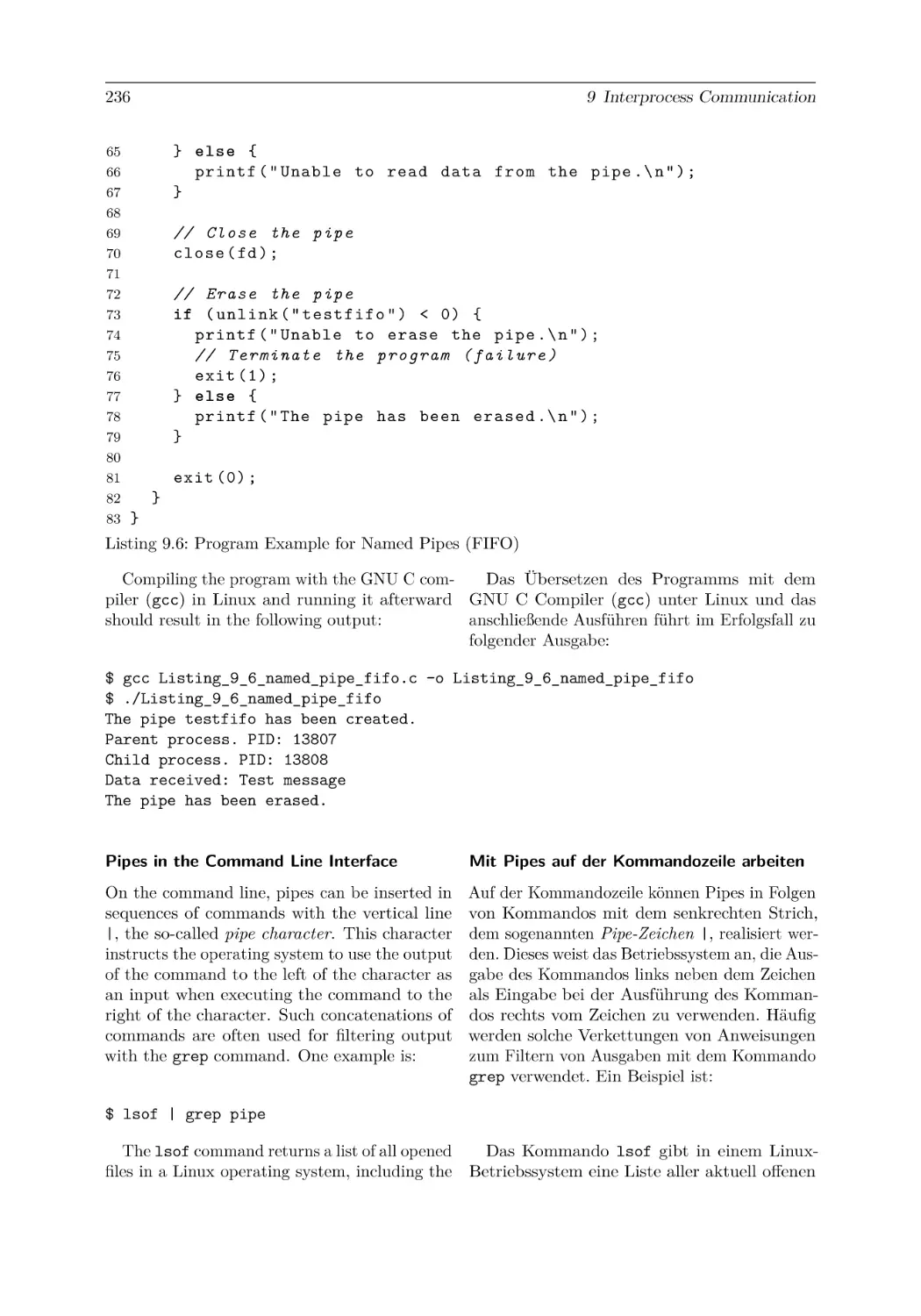
9.3.5 Pipes . . . . . . . . . . . . . . . . . . . . . . . .
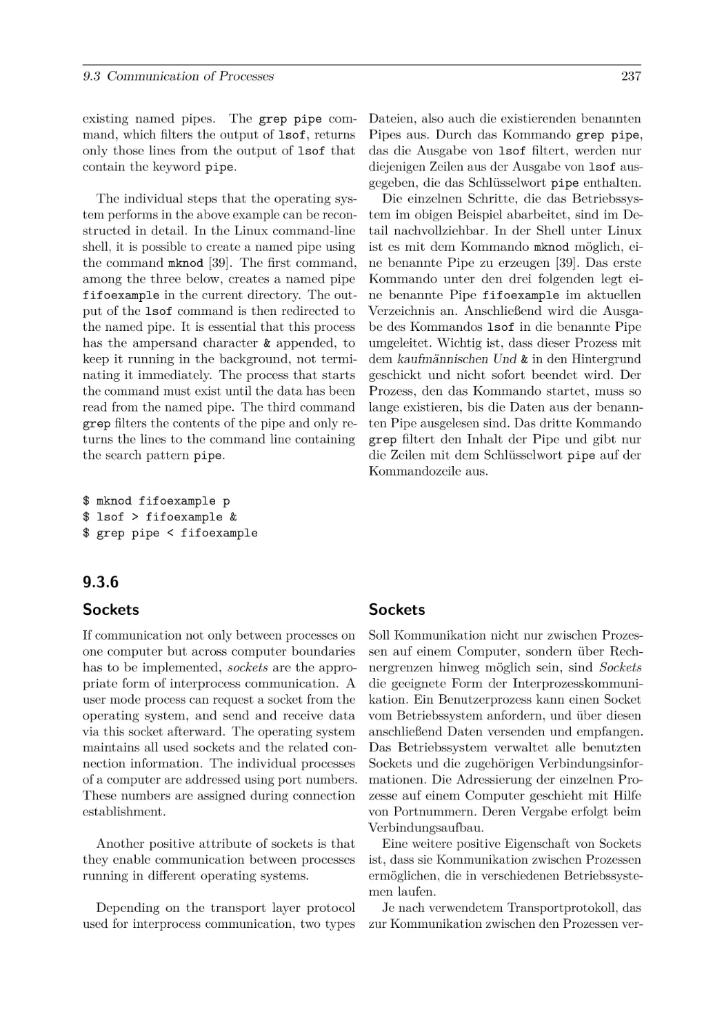
9.3.6 Sockets . . . . . . . . . . . . . . . . . . . . . . .
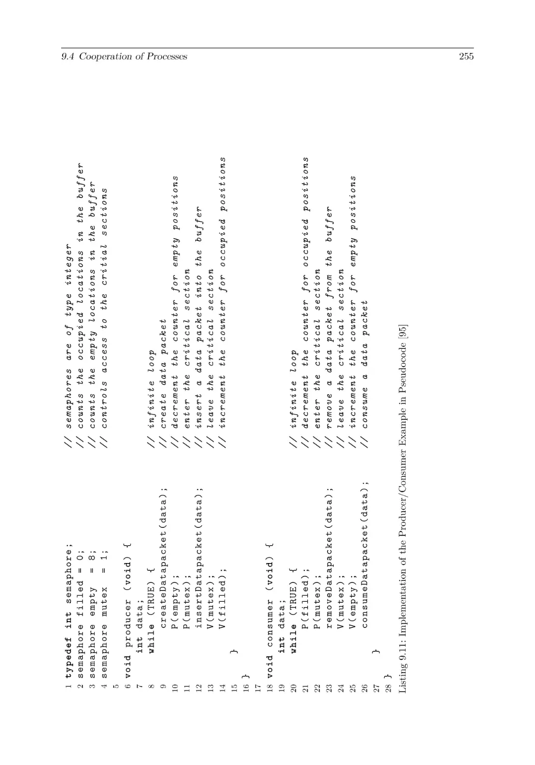
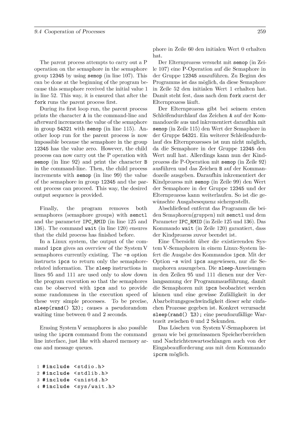
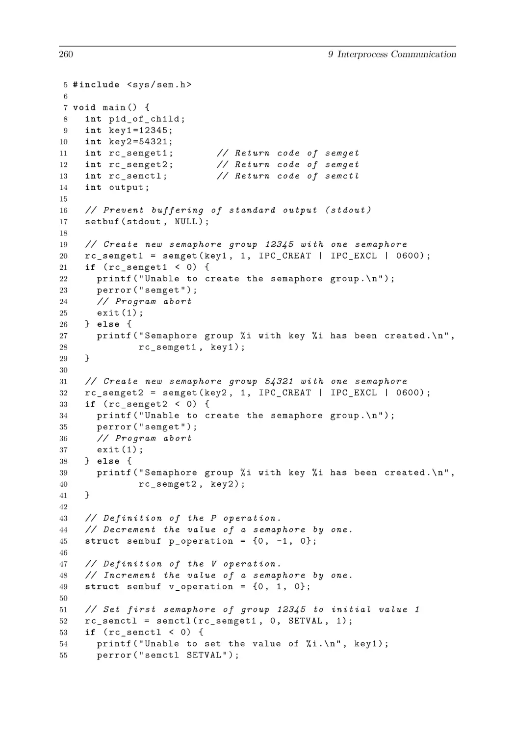
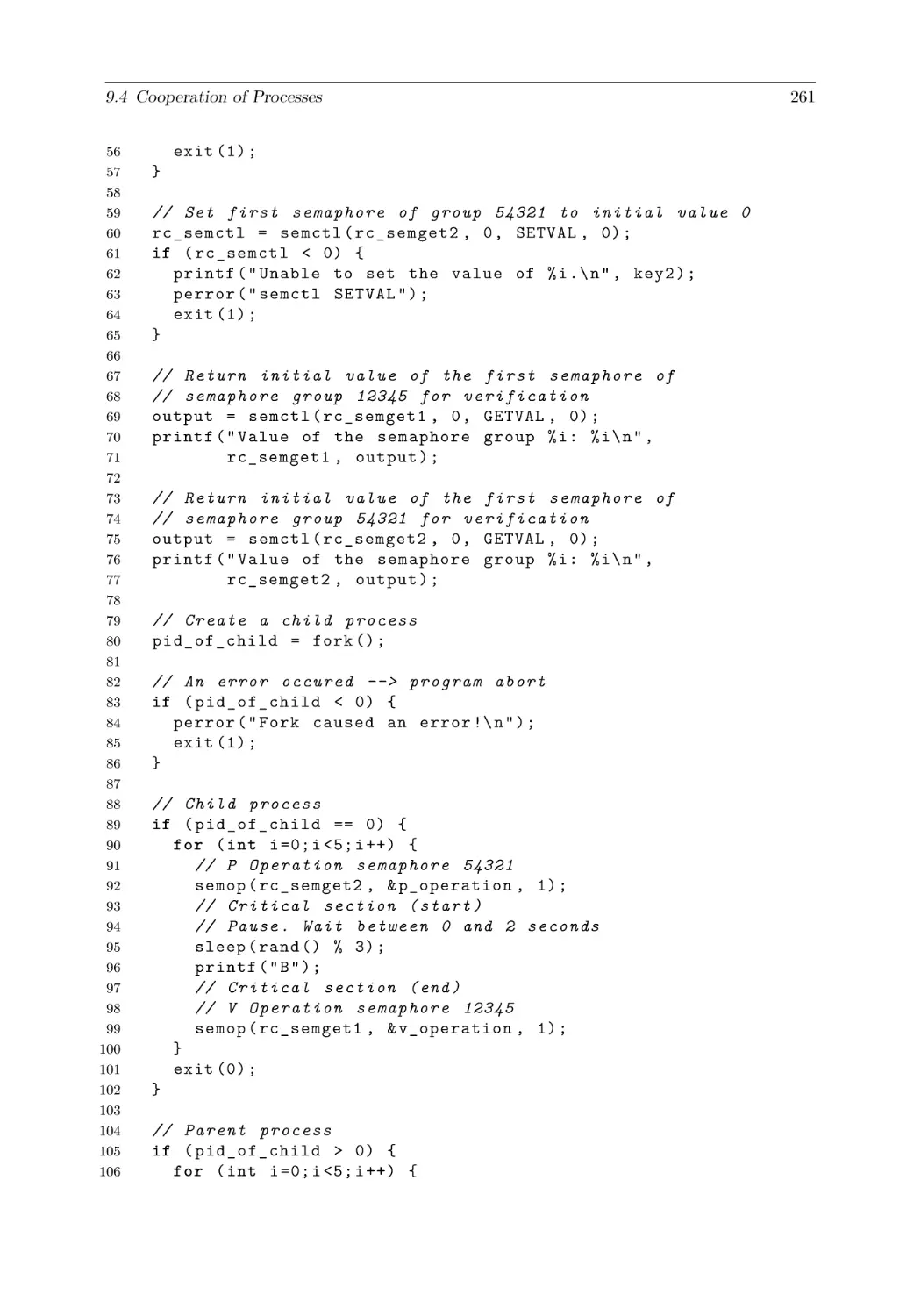
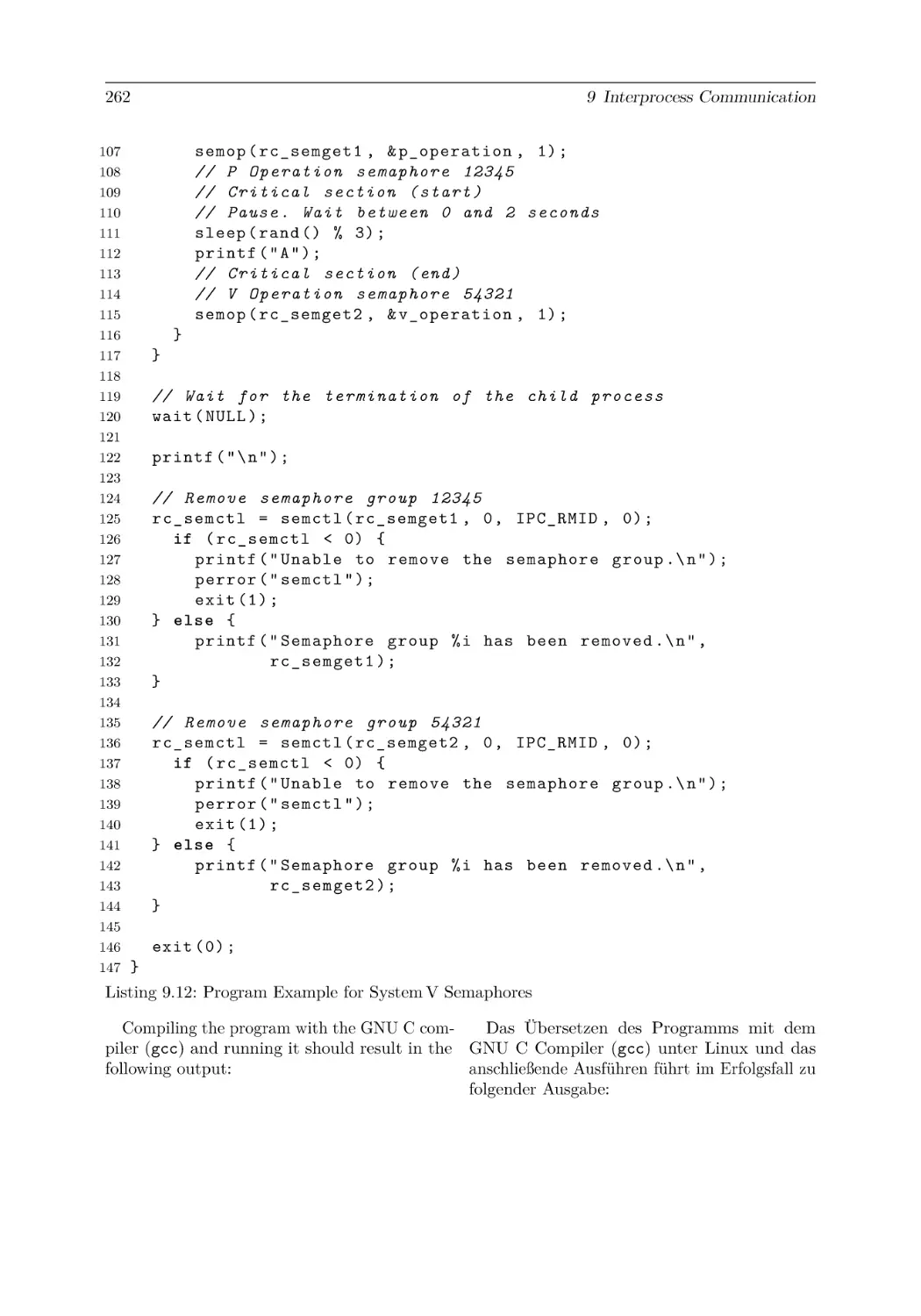
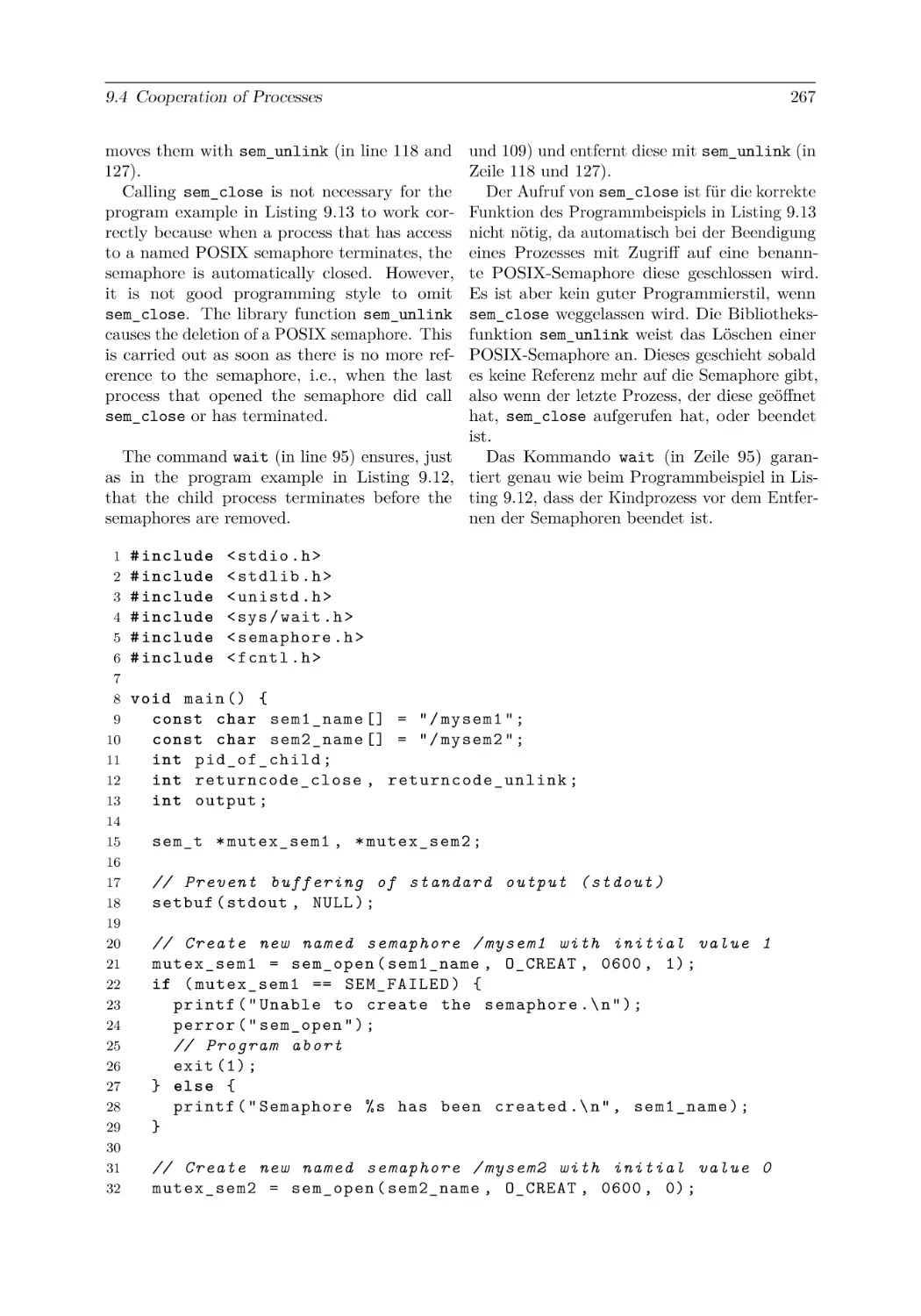
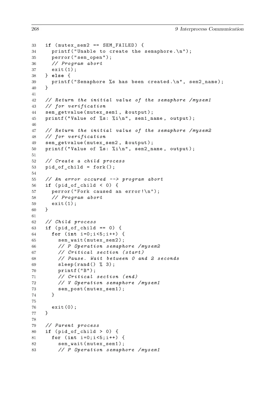
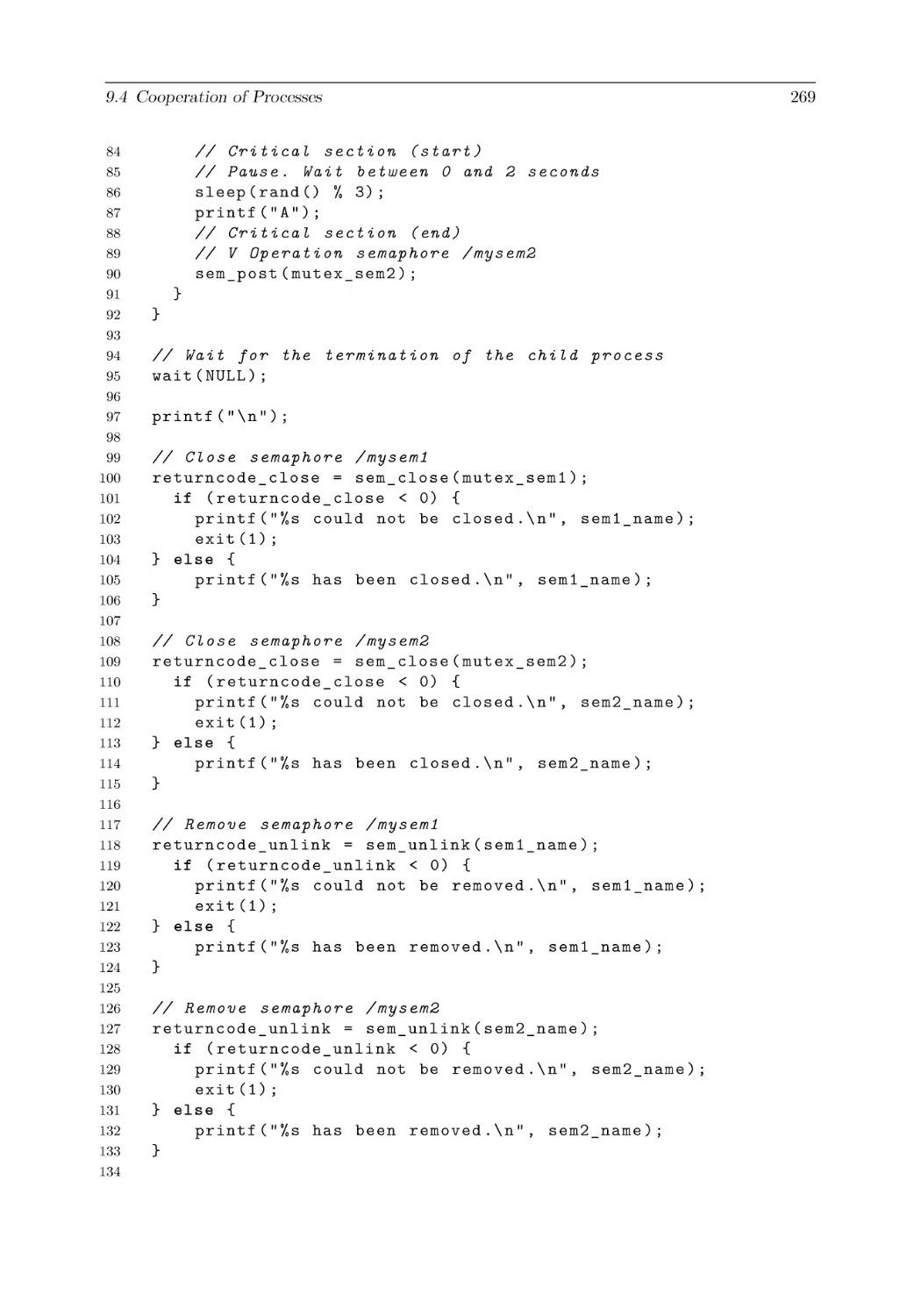
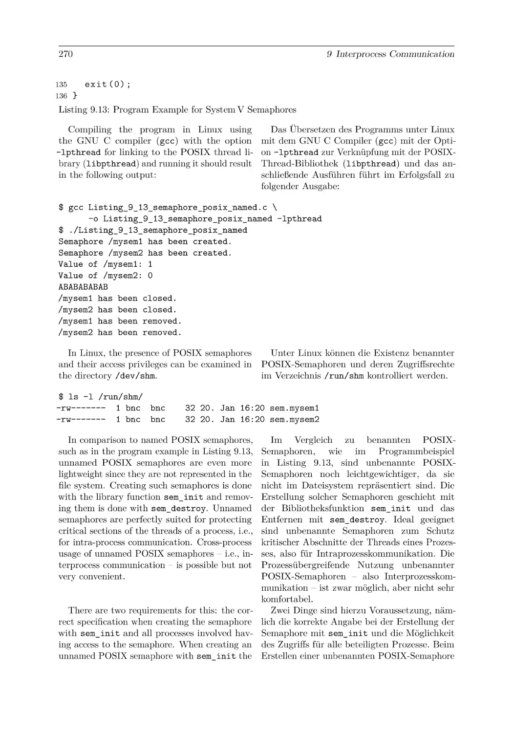
9.4 Cooperation of Processes . . . . . . . . . . . . . . . . .

.
.
.
.
.
.
.
.
.
.
.
.
.

195
195
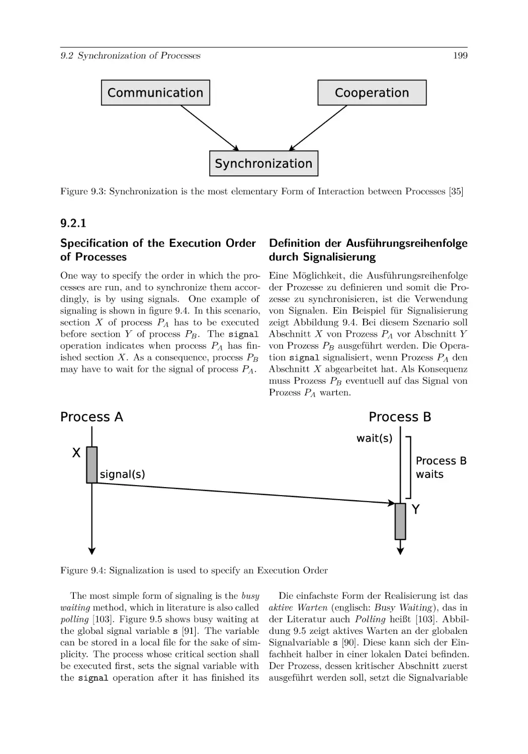
198
199
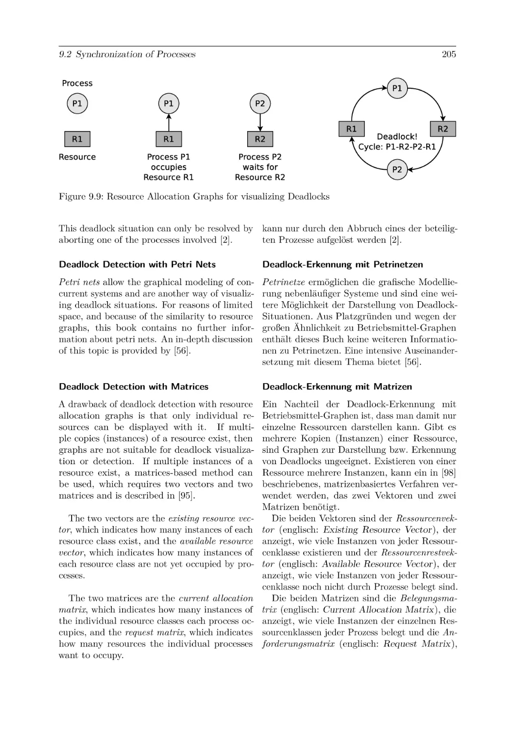
201
203
208
208
214
218
225
230
237
252

.
.
.
.
.
.
.
.
.
.
.
.
.
.
.
.
.
.

xii

Contents
9.4.1
9.4.2
9.4.3
9.4.4
9.4.5

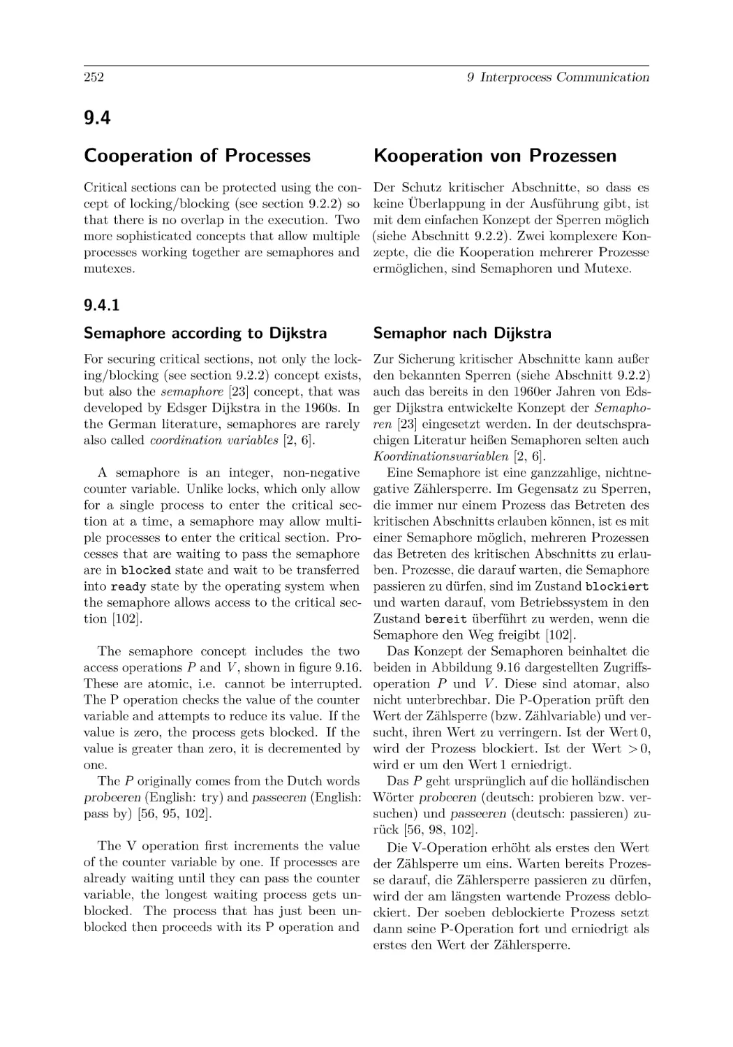
Semaphore according to Dijkstra
Semaphores (System V) . . . . .
Semaphores (POSIX) . . . . . .
Mutex . . . . . . . . . . . . . . .
Monitor . . . . . . . . . . . . . .

.
.
.
.
.

252
256
264
271
273

10 Virtualization
10.1 Partitioning . . . . . . . . . . . . . . .
10.2 Hardware Emulation . . . . . . . . . .
10.3 Application Virtualization . . . . . . .
10.4 Full Virtualization . . . . . . . . . . .
10.5 Paravirtualization . . . . . . . . . . . .
10.6 Hardware Virtualization . . . . . . . .
10.7 Operating System-level Virtualization .

.
.
.
.
.
.
.

275
275
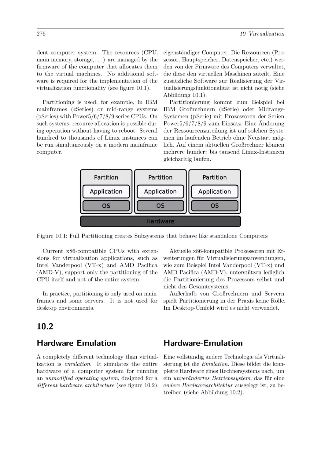
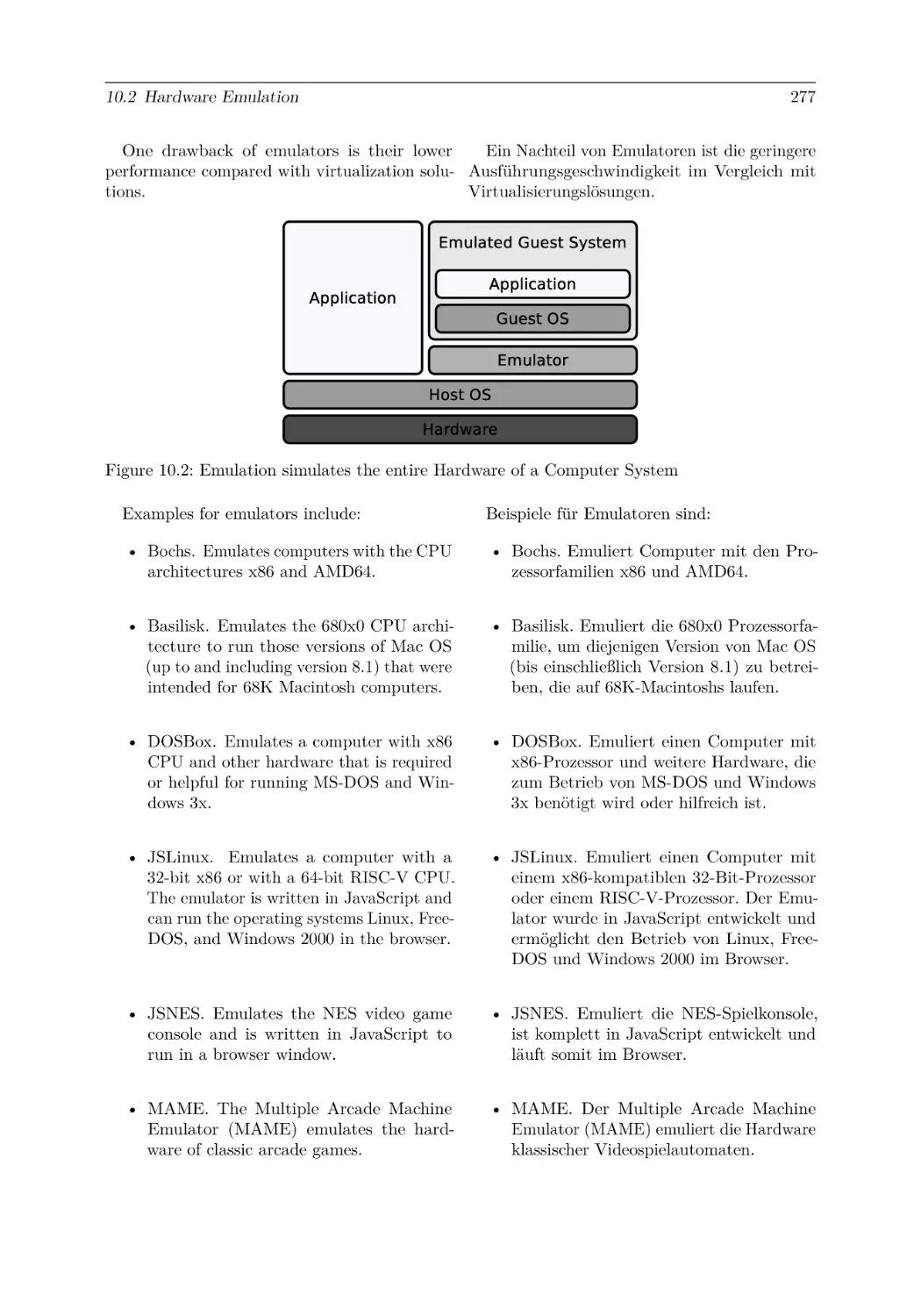
276
278
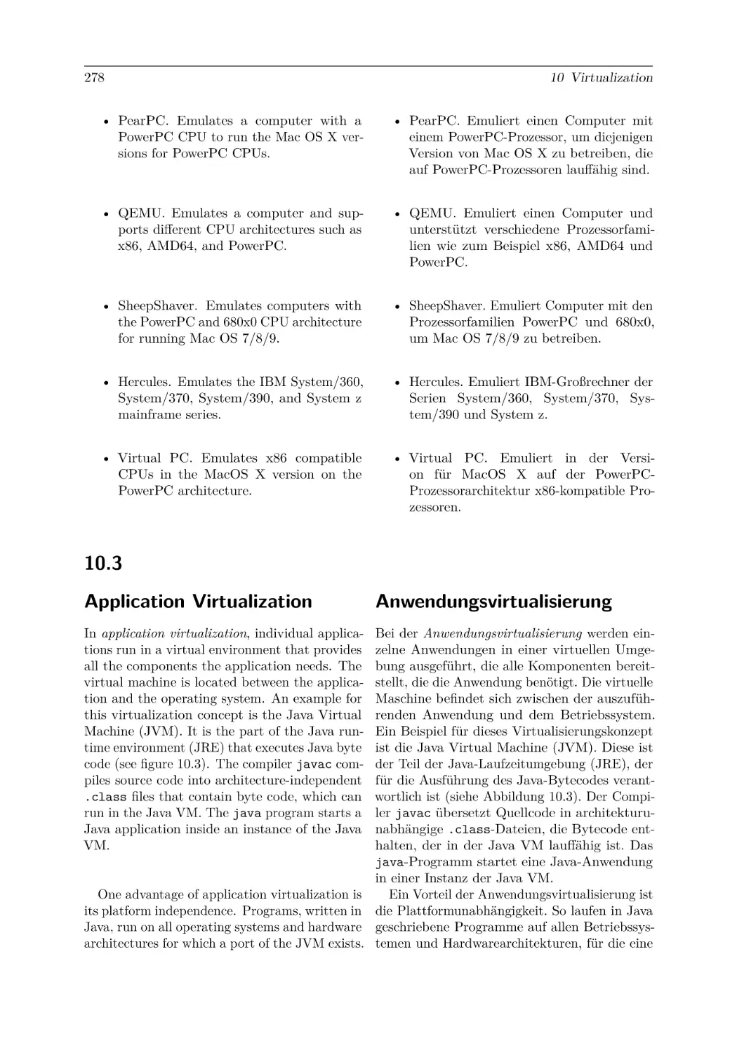
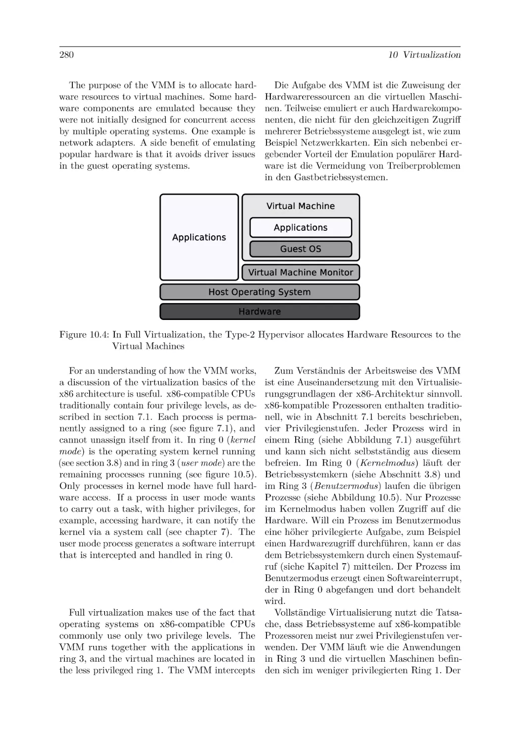
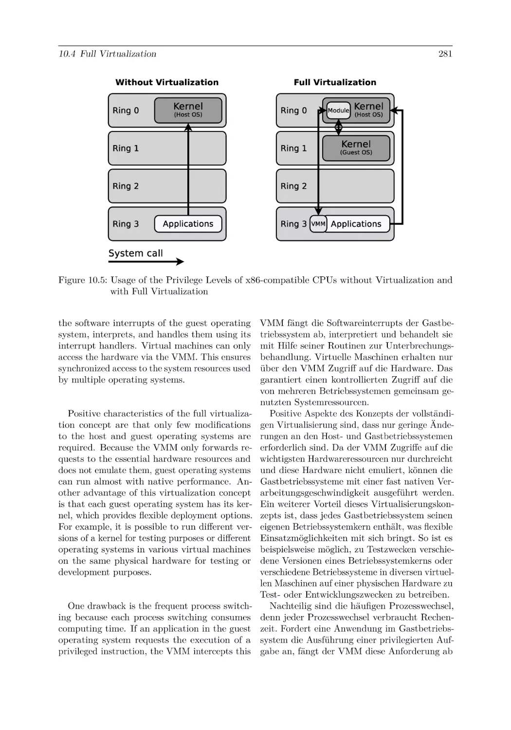
279
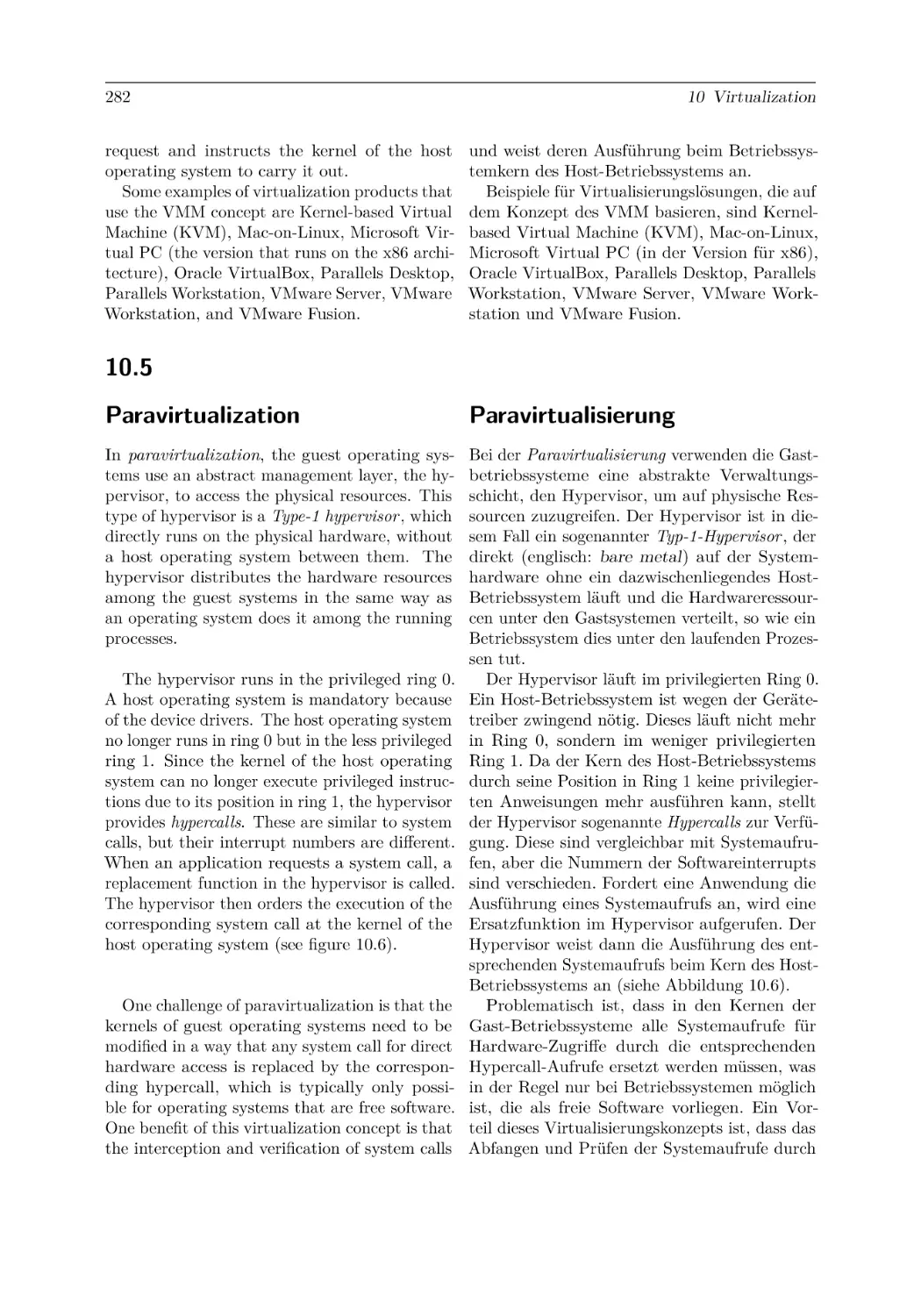
282
283
284

Glossary

287

References

301

Index

307

Inhaltsverzeichnis
1 Einleitung
2 Grundlagen der Informationstechnik
2.1 Bit . . . . . . . . . . . . . . . . .
2.2 Repräsentation von Zahlen . . .
2.2.1 Dezimalsystem . . . . . .
2.2.2 Dualsystem . . . . . . . .
2.2.3 Oktalsystem . . . . . . . .
2.2.4 Hexadezimalsystem . . . .
2.3 Datei- und Speichergrößen . . . .
2.4 Informationsdarstellung . . . . .
2.4.1 ASCII-Kodierung . . . . .
2.5 Unicode . . . . . . . . . . . . . .
2.6 Darstellung von Zeichenketten .

1
.
.
.
.
.
.
.
.
.
.
.

.
.
.
.
.
.
.
.
.
.
.

3
3
4
5
5
6
7
8
9
10
12
13

3 Grundlagen der Betriebssysteme
3.1 Einordnung der Betriebssysteme in die Informatik . . . . . . .
3.2 Positionierung und Kernfunktionalitäten von Betriebssystemen
3.3 Entwicklung der Betriebssysteme . . . . . . . . . . . . . . . . .
3.3.1 Zweite Generation von Computern . . . . . . . . . . . .
3.3.2 Dritte Generation von Computern . . . . . . . . . . . .
3.3.3 Vierte Generation von Computern . . . . . . . . . . . .
3.4 Betriebsarten . . . . . . . . . . . . . . . . . . . . . . . . . . . .
3.4.1 Stapelbetrieb und Dialogbetrieb . . . . . . . . . . . . .
3.4.2 Einzelprogrammbetrieb und Mehrprogrammbetrieb . . .
3.4.3 Einzelbenutzerbetrieb und Mehrbenutzerbetrieb . . . .
3.5 8/16/32/64-Bit-Betriebssysteme . . . . . . . . . . . . . . . . .
3.6 Echtzeitbetriebssysteme . . . . . . . . . . . . . . . . . . . . . .
3.6.1 Harte und weiche Echtzeitbetriebssysteme . . . . . . . .
3.6.2 Architekturen von Echtzeitbetriebssystemen . . . . . . .
3.7 Verteilte Betriebssysteme . . . . . . . . . . . . . . . . . . . . .
3.8 Architektur des Betriebssystemkerns . . . . . . . . . . . . . . .
3.8.1 Monolithische Kerne . . . . . . . . . . . . . . . . . . . .
3.8.2 Minimale Kerne . . . . . . . . . . . . . . . . . . . . . . .
3.8.3 Hybride Kerne . . . . . . . . . . . . . . . . . . . . . . .
3.9 Schichtenmodell . . . . . . . . . . . . . . . . . . . . . . . . . .

.
.
.
.
.
.
.
.
.
.
.
.
.
.
.
.
.
.
.
.

15
15
16
19
20
21
22
23
23
25
26
27
28
28
29
30
32
34
34
36
37

4 Grundlagen der Rechnerarchitektur
4.1 Von-Neumann-Architektur . . . . . . . . . . . . . . . . . . . . . . . . . . . . . . .
4.1.1 Hauptprozessor . . . . . . . . . . . . . . . . . . . . . . . . . . . . . . . . . .
4.1.2 Von-Neumann-Zyklus . . . . . . . . . . . . . . . . . . . . . . . . . . . . . .

39
39
40
41

.
.
.
.
.
.
.
.
.
.
.

xiv

Inhaltsverzeichnis
4.1.3 Busleitungen . . . . . . . . . . . . . . .
4.2 Ein-/Ausgabegeräte . . . . . . . . . . . . . . .
4.3 Digitale Datenspeicher . . . . . . . . . . . . . .
4.4 Speicherhierarchie . . . . . . . . . . . . . . . .
4.4.1 Register . . . . . . . . . . . . . . . . . .
4.4.2 Cache . . . . . . . . . . . . . . . . . . .
4.4.3 Cache-Schreibstrategien . . . . . . . . .
4.4.4 Hauptspeicher . . . . . . . . . . . . . .
4.4.5 Festplatten . . . . . . . . . . . . . . . .
4.4.6 Adressierung der Daten auf Festplatten
4.4.7 Zugriﬀszeit bei Festplatten . . . . . . .
4.4.8 Solid-State Drives . . . . . . . . . . . .
4.4.9 Daten aus Flash-Speicherzellen auslesen
4.5 RAID . . . . . . . . . . . . . . . . . . . . . . .
4.5.1 RAID 0 . . . . . . . . . . . . . . . . . .
4.5.2 RAID 1 . . . . . . . . . . . . . . . . . .
4.5.3 RAID 2 . . . . . . . . . . . . . . . . . .
4.5.4 RAID 3 . . . . . . . . . . . . . . . . . .
4.5.5 RAID 4 . . . . . . . . . . . . . . . . . .
4.5.6 RAID 5 . . . . . . . . . . . . . . . . . .
4.5.7 RAID 6 . . . . . . . . . . . . . . . . . .
4.5.8 RAID-Kombinationen . . . . . . . . . .

.
.
.
.
.
.
.
.
.
.
.
.
.
.
.
.
.
.
.
.
.
.

42
45
48
49
52
52
53
54
55
56
58
58
60
64
67
68
69
70
71
72
73
73

5 Speicherverwaltung
5.1 Konzepte zur Speicherverwaltung . . . . . . . . . . .
5.1.1 Statische Partitionierung . . . . . . . . . . . .
5.1.2 Dynamische Partitionierung . . . . . . . . . .
5.1.3 Buddy-Speicherverwaltung . . . . . . . . . .
5.2 Speicheradressierung in der Praxis . . . . . . . . . .
5.2.1 Real Mode . . . . . . . . . . . . . . . . . . .
5.2.2 Protected Mode und virtueller Speicher . . .
5.2.3 Seitenorientierter Speicher (Paging) . . . . .
5.2.4 Segmentorientierter Speicher (Segmentierung)
5.2.5 Stand der Technik beim virtuellen Speicher .
5.2.6 Kernelspace und Userspace . . . . . . . . . .
5.3 Seitenersetzungsstrategien . . . . . . . . . . . . . . .
5.3.1 Optimale Strategie . . . . . . . . . . . . . . .
5.3.2 Least Recently Used . . . . . . . . . . . . . .
5.3.3 Least Frequently Used . . . . . . . . . . . . .
5.3.4 First In First Out . . . . . . . . . . . . . . .
5.3.5 Clock / Second Chance . . . . . . . . . . . .
5.3.6 Random . . . . . . . . . . . . . . . . . . . . .

.
.
.
.
.
.
.
.
.
.
.
.
.
.
.
.
.
.

75
75
76
77
79
83
84
88
90
99
100
102
103
104
105
106
107
108
109

6 Dateisysteme
6.1 Technische Grundlagen der Dateisysteme .
6.2 Blockadressierung bei Linux-Dateisystemen
6.2.1 Minix . . . . . . . . . . . . . . . . .
6.2.2 ext2/3/4 . . . . . . . . . . . . . . . .
6.3 Dateisysteme mit Dateizuordnungstabellen
6.3.1 FAT12 . . . . . . . . . . . . . . . . .
6.3.2 FAT16 . . . . . . . . . . . . . . . . .
6.3.3 FAT32 . . . . . . . . . . . . . . . . .

.
.
.
.
.
.
.
.

111
111
112
115
117
120
124
124
126

.
.
.
.
.
.
.
.

.
.
.
.
.
.
.
.
.
.
.
.
.
.
.
.
.
.
.
.
.
.

.
.
.
.
.
.
.
.

.
.
.
.
.
.
.
.
.
.
.
.
.
.
.
.
.
.
.
.
.
.

.
.
.
.
.
.
.
.

Inhaltsverzeichnis
.
.
.
.
.
.
.
.
.
.
.
.

126
127
130
131
133
135
138
138
140
140
141
142

7 Systemaufrufe
7.1 Benutzermodus und Kernelmodus . . . . . . . . . . . . . . . . . . . . . . . . . . .
7.2 Systemaufrufe und Bibliotheken . . . . . . . . . . . . . . . . . . . . . . . . . . . .
7.3 Ablauf eines Systemaufrufs . . . . . . . . . . . . . . . . . . . . . . . . . . . . . . .

145
145
146
150

8 Prozessverwaltung
8.1 Prozesskontext . . . . . . . . . . . . . . . . . . . .
8.2 Prozesszustände . . . . . . . . . . . . . . . . . . .
8.3 Struktur eines Prozesses im Speicher . . . . . . . .
8.4 Prozesse erzeugen mit fork . . . . . . . . . . . . .
8.5 Prozesse ersetzen mit exec . . . . . . . . . . . . . .
8.6 Prozesswechsel und Scheduling von Prozessen . . .
8.6.1 Prioritätengesteuertes Scheduling . . . . . .
8.6.2 First Come First Served . . . . . . . . . . .
8.6.3 Round Robin . . . . . . . . . . . . . . . . .
8.6.4 Shortest Job First / Shortest Process Next
8.6.5 Shortest Remaining Time First . . . . . . .
8.6.6 Longest Job First . . . . . . . . . . . . . . .
8.6.7 Longest Remaining Time First . . . . . . .
8.6.8 Highest Response Ratio Next . . . . . . . .
8.6.9 Earliest Deadline First . . . . . . . . . . . .
8.6.10 Fair-Share-Scheduling . . . . . . . . . . . .
8.6.11 Multilevel-Scheduling . . . . . . . . . . . .
8.6.12 Scheduling von Linux-Betriebssystemen . .

.
.
.
.
.
.
.
.
.
.
.
.
.
.
.
.
.
.

153
153
155
162
165
171
175
177
178
179
180
181
182
182
183
183
184
185
187

9 Interprozesskommunikation
9.1 Kritische Abschnitte und Wettlaufsituationen . . .
9.2 Synchronisation von Prozessen . . . . . . . . . . .
9.2.1 Deﬁnition der Ausführungsreihenfolge durch
9.2.2 Schutz kritischer Abschnitte durch Sperren
9.2.3 Verhungern und Deadlock . . . . . . . . . .
9.3 Kommunikation von Prozessen . . . . . . . . . . .
9.3.1 Gemeinsamer Speicher (System V) . . . . .
9.3.2 POSIX-Speichersegmente . . . . . . . . . .
9.3.3 Nachrichtenwarteschlangen (System V) . . .
9.3.4 POSIX-Nachrichtenwarteschlangen . . . . .
9.3.5 Kommunikationskanäle . . . . . . . . . . .
9.3.6 Sockets . . . . . . . . . . . . . . . . . . . .
9.4 Kooperation von Prozessen . . . . . . . . . . . . .

. . . . . . . . .
. . . . . . . . .
Signalisierung
. . . . . . . . .
. . . . . . . . .
. . . . . . . . .
. . . . . . . . .
. . . . . . . . .
. . . . . . . . .
. . . . . . . . .
. . . . . . . . .
. . . . . . . . .
. . . . . . . . .

.
.
.
.
.
.
.
.
.
.
.
.
.

195
195
198
199
201
203
208
208
214
218
225
230
237
252

6.4
6.5

6.6

6.7
6.8

6.3.4 VFAT . . . . . . . . . . . . . . . . . .
6.3.5 exFAT . . . . . . . . . . . . . . . . . .
Journaling-Dateisysteme . . . . . . . . . . . .
Extent-basierte Adressierung . . . . . . . . .
6.5.1 ext4 . . . . . . . . . . . . . . . . . . .
6.5.2 NTFS . . . . . . . . . . . . . . . . . .
Copy-on-Write . . . . . . . . . . . . . . . . .
6.6.1 ZFS . . . . . . . . . . . . . . . . . . .
6.6.2 Btrfs . . . . . . . . . . . . . . . . . . .
6.6.3 ReFS . . . . . . . . . . . . . . . . . .
Datenzugriﬀe mit einem Cache beschleunigen
Defragmentierung . . . . . . . . . . . . . . .

xv
.
.
.
.
.
.
.
.
.
.
.
.

.
.
.
.
.
.
.
.
.
.
.
.

.
.
.
.
.
.
.
.
.
.
.
.
.
.
.
.
.
.

.
.
.
.
.
.
.
.
.
.
.
.

.
.
.
.
.
.
.
.
.
.
.
.
.
.
.
.
.
.

.
.
.
.
.
.
.
.
.
.
.
.

.
.
.
.
.
.
.
.
.
.
.
.
.
.
.
.
.
.

.
.
.
.
.
.
.
.
.
.
.
.

.
.
.
.
.
.
.
.
.
.
.
.
.
.
.
.
.
.

.
.
.
.
.
.
.
.
.
.
.
.

.
.
.
.
.
.
.
.
.
.
.
.
.
.
.
.
.
.

.
.
.
.
.
.
.
.
.
.
.
.

.
.
.
.
.
.
.
.
.
.
.
.
.
.
.
.
.
.

.
.
.
.
.
.
.
.
.
.
.
.

.
.
.
.
.
.
.
.
.
.
.
.
.
.
.
.
.
.

.
.
.
.
.
.
.
.
.
.
.
.

xvi

Inhaltsverzeichnis
9.4.1
9.4.2
9.4.3
9.4.4
9.4.5

Semaphor nach Dijkstra
Semaphoren (System V)
POSIX-Semaphoren . .
Mutex . . . . . . . . . .
Monitor . . . . . . . . .

.
.
.
.
.

252
256
264
271
273

10 Virtualisierung
10.1 Partitionierung . . . . . . . . .
10.2 Hardware-Emulation . . . . . .
10.3 Anwendungsvirtualisierung . . .
10.4 Vollständige Virtualisierung . .
10.5 Paravirtualisierung . . . . . . .
10.6 Hardware-Virtualisierung . . . .
10.7 Betriebssystem-Virtualisierung .

.
.
.
.
.
.
.

275
275
276
278
279
282
283
284

Glossar

287

Literatur

301

Index / Stichwortverzeichnis

307

1
Introduction

Einleitung

This book intends to provide a compact, but
not a comprehensive overview of operating systems and their components. The aim is to assist
its readers in gaining a basic understanding of
the way operating systems and their components work. No prior technical knowledge is
required.

Dieses Buch will einen Überblick über das
Thema Betriebssysteme und deren Komponenten schaﬀen, ohne dabei den Anspruch auf Vollständigkeit zu erheben. Das Ziel ist es, den Leserinnen und Lesern ein grundlegendes Wissen
über die Funktionsweise von Betriebssystemen
und deren Komponenten zu vermitteln. Technische Vorkenntnisse sind dabei nicht erforderlich.
In den Kapiteln 2 und 3 ﬁndet eine Einführung in die Grundlagen der Informationstechnik
und der Betriebssysteme statt. Dies ist nötig,
um die Thematik Betriebssysteme und den Inhalt dieses Buchs verstehen zu können.
Ein Verständnis der notwendigsten Hardwarekomponenten eines Computers ist elementar,
um die Arbeitsweise von Betriebssystemen zu
verstehen. Darum beschäftigt sich Kapitel 4
mit den Grundlagen der Rechnerarchitektur.
Schwerpunkte dieses Kapitels sind die Arbeitsweise des Hauptprozessors, des Speichers und
der Bussysteme.
Kapitel 5 beschreibt die grundlegenden Konzepte der Speicherverwaltung und die Art und
Weise, wie moderne Betriebssysteme den Cache
und den Hauptspeicher verwalten.
Eine andere Form der Speicherverwaltung thematisiert Kapitel 6. Dieses Kapitel beschreibt
die technischen Grundlagen klassischer und moderner Dateisysteme anhand ausgewählter Beispiele.
Die Interaktion der Benutzerprozesse mit den
Funktionen des Betriebssystemkerns geschieht
via Systemaufrufe. Diese können direkt oder
über Bibliotheksfunktionen aufgerufen werden.
Eine Beschreibung der Arbeitsweise von und
mit Systemaufrufen enthält Kapitel 7.
Der Fokus von Kapitel 8 liegt auf der Prozessverwaltung. Schwerpunkte sind einerseits die
Art und Weise, wie Prozesse im Betriebssystem
realisiert werden und nach welchen Kriterien
diese den Prozessor zugewiesen bekommen.

The chapters 2 and 3 provide an introduction
to the fundamentals of information technology
(IT) and operating systems. These topics are
necessary to understand operating systems and
the contents of this book.
An understanding of the main hardware components of a computer is essential to understand
how operating systems work. Therefore, chapter 4 deals with the basics of computer architecture. This chapter focuses on the way the CPU,
the memory, and the bus systems work.

Chapter 5 describes the fundamental concepts
of memory management and the way modern
operating systems organize the cache and the
main memory.
Chapter 6 deals with another form of memory
management. This chapter describes the technical basics of classic and modern ﬁle systems
using various examples.
The user processes interact with the functions
of the operating system kernel via system calls.
These are called directly or via library functions.
A description of the functioning of system calls
and how to use them is included in chapter 7.
The focus of chapter 8 is on process management. The topics of this chapter are, among
others, the implementation of processes by the
operating system, and the criteria by which they
are assigned to the CPU.

© Springer Fachmedien Wiesbaden GmbH, ein Teil von Springer Nature 2023
C. Baun, Operating Systems / Betriebssysteme,
https://doi.org/10.1007/978-3-658-42230-1_1

2
Possible ways for protecting critical sections
and the various aspects of interprocess communication are described in chapter 9.
Finally, chapter 10 provides an introduction
to the virtualization concepts that are relevant
for operating systems.

1 Introduction
Möglichkeiten zum Schutz kritischer Abschnitte und die verschiedenen Aspekte der Interprozesskommunikation beschreibt Kapitel 9.
Abschließend ﬁndet in Kapitel 10 eine Einführung in die aus Sicht der Betriebssysteme
relevanten Virtualisierungskonzepte statt.

2
Fundamentals of
Computer Science

Grundlagen der
Informationstechnik

A basic understanding of information technology (IT) is required to understand how
operating systems work. These fundamentals
include the variants of information representation, and the representation of numbers, orders
of magnitude, and the way information (especially textual information) are represented in
computers.

Um die Funktionsweise von Betriebssystemen
zu verstehen, ist ein grundlegendes Verständnis
der Informationstechnik (IT) nötig. Bei diesen
Grundlagen handelt es sich um die Möglichkeiten der Informationsdarstellung und Repräsentation von Zahlen, Größenordnungen und die
Art und Weise, wie Informationen (speziell Texte) in Rechnern dargestellt werden.

2.1
Bit

Bit

A bit is the smallest possible unit of information,
and every piece of information is bound to an
information carrier [32]. An information carrier,
which can have one of two states, can represent
one bit of data. The value of one or more bits
is called state. One bit can represent two states.
Diﬀerent scenarios can represent one bit of data.
Examples are:

Ein Bit ist die kleinstmögliche Einheit der Information und jede Information ist an einen
Informationsträger gebunden [32]. Ein Informationsträger, der sich in genau einem von zwei
Zuständen beﬁnden kann, kann die Datenmenge
1 Bit darstellen. Den Wert eines oder mehrerer
Bits nennt man Zustand. Ein Bit kann zwei
Zustände darstellen. Verschiedene Sachverhalte
können die Datenmenge 1 Bit darstellen. Beispiele sind:

• The position of a switch with two states

• Die Stellung eines Schalters mit zwei Zuständen

• The switching state of a transistor

• Der Schaltzustand eines Transistors

• The presence of an electrical voltage or
charge

• Das Vorhandensein einer elektrischen
Spannung oder Ladung

• The presence of magnetization

• Das Vorhandensein einer Magnetisierung

© Springer Fachmedien Wiesbaden GmbH, ein Teil von Springer Nature 2023
C. Baun, Operating Systems / Betriebssysteme,
https://doi.org/10.1007/978-3-658-42230-1_2

2 Fundamentals of Computer Science
• The value of a variable with logical truth
values

• Der Wert einer Variable mit den logischen
Wahrheitswerten

If more than two states are required to store
information, multiple bits (bit sequences) are
needed. With n bits, it is possible to represent 2n diﬀerent states (see table 2.1). With
2 bits, 22 = 4 diﬀerent states can be represented, namely 00, 01, 10, and 11. With 3 bits,
23 = 8 diﬀerent states (000, 001, 010, 011, 100,
101, 110, and 111) can be represented. With
each additional bit, the number of representable
states (bit sequences) doubles [32].

Benötigt man zur Speicherung einer Information mehr als zwei Zustände, sind Folgen von
Bits (Bitfolgen) nötig. Mit n Bits kann man 2n
verschiedene Zustände darstellen (siehe Tabelle 2.1). Also kann man mit 2 Bits 22 = 4 verschiedene Zustände repräsentieren, nämlich 00,
01, 10 und 11. Mit 3 Bits kann man schon 23 = 8
verschiedene Zustände (000, 001, 010, 011, 100,
101, 110 und 111) repräsentieren. Jedes zusätzliche Bit verdoppelt die Anzahl der möglichen
darstellbaren Zustände (Bitfolgen) [32].

Table 2.1: The Number of representable States doubles with each additional Bit
Bits
1
2
3
4
5
6
7
8

States
1

2 =2
22 = 4
23 = 8
24 = 16
25 = 32
26 = 64
27 = 128
28 = 256

Bits
9
10
11
12
13
14
15
16

States
9

2 = 512
210 = 1,024
211 = 2,048
212 = 4,096
213 = 8,192
214 = 16,384
215 = 32,768
216 = 65,536

Bits

States

17
18
19
20
21
22
23
24

217 = 131,072
218 = 262,144
219 = 524,288
220 = 1,048,576
221 = 2,097,152
222 = 4,194,304
223 = 8,388,608
224 = 16,777,216

2.2
Representation of Numbers

Repräsentation von Zahlen

Numbers can be represented in various ways.
One task of IT is to map numbers from the
real world to the computer. In this context, the
distinction between value and representation is
signiﬁcant.
In mathematics, numbers are distinguished
as elements of diﬀerent sets of values (natural
numbers, integers, real numbers, complex numbers, . . . ). The value of a number is also called
abstract number, and its value is independent of
the representation (for example, 0.5 = 1/2).

Zahlen kann man auf unterschiedliche Arten
darstellen. Eine Aufgabe der IT ist es, Zahlen
aus der realen Welt im Computer abzubilden.
Wichtig ist dabei die Unterscheidung zwischen
Wert und Darstellung.
In der Mathematik unterscheidet man Zahlen als Elemente verschiedener Wertemengen
(natürliche Zahlen, ganze Zahlen, reelle Zahlen,
komplexe Zahlen, usw.). Den Wert einer Zahl
nennt man auch abstrakte Zahl und der Wert ist
unabhängig von der Darstellung (zum Beispiel
0,5 = 1/2).
Operationen eines Rechners werden aber nicht
auf Werten, sondern auf Bitfolgen ausgeführt.
Darum ist für die IT besonders die Darstellung der Zahlen interessant. Die Darstellung
wird vom verwendeten Stellenwertsystem (Positionssystem) bestimmt. Die für die IT wichtigen

However, operations of a computer are not
executed on values, but on bit sequences. This
is why the representation of numbers is particularly interesting for IT. The representation is
determined by the place value system (positional
notation). Relevant for IT are the decimal sys-

2.2 Representation of Numbers
tem, the binary system, the octal system, and
the hexadecimal system.

5
Stellenwertsysteme sind das Dezimalsystem, das
Dualsystem, das Oktalsystem und das Hexadezimalsystem.

2.2.1
Dezimalsystem

Decimal System

The decimal system uses the number 10 as base. Das Dezimalsystem verwendet als Basis die
Each digit D at the position i has the value Zahl 10. Jede Ziﬀer D an der Stelle i hat den
D × 10i . One example is:
Wert D × 10i . Ein Beispiel ist:
2013 = 2 × 103 + 0 × 102 + 1 × 101 + 3 × 100
Computer systems distinguish between two
electrical states. Therefore, the number 2 as
base; hence, the binary system is ideal for IT.

Computer-Systeme unterscheiden prinzipiell
zwischen zwei elektrischen Zuständen. Darum
ist aus Sicht der IT als Basis die Zahl 2 und
damit das Dualsystem optimal geeignet.

2.2.2
Binary System

Dualsystem

The binary system uses the number 2 as base.
Numbers are represented by using the digits
of the values zero and one. Number representations in the binary system are called binary
numbers. All positive natural numbers, including zero, can be represented by sequences of
symbols from the set {0, 1}. If n is the number
of bits, x0 is the least signiﬁcant bit (LSB), and
xn−1 is the most signiﬁcant bit (MSB).

Das Dualsystem verwendet als Basis die Zahl 2.
Zahlen werden nur mit den Ziﬀern der Werte
Null und Eins dargestellt. Zahldarstellungen im
Dualsystem heißen Dualzahlen oder Binärzahlen. Alle positiven natürlichen Zahlen inklusive
der Null können durch Folgen von Symbolen aus
der Menge {0, 1} repräsentiert werden. Wenn n
der Anzahl der Bits entspricht, ist x0 das niederwertigste Bit (Least Signiﬁcant Bit – LSB) und
xn−1 das höchstwertigste Bit (Most Signiﬁcant
Bit – MSB).
Da lange Reihen von Nullen und Einsen für
Menschen schnell unübersichtlich werden, verwendet man zur Darstellung von Bitfolgen häuﬁg das Oktalsystem oder das Hexadezimalsystem.
Die Umrechnung der Stellenwertsysteme ist
einfach möglich. Zur Verdeutlichung ist das Stellenwertsystem der jeweiligen Zahl in den folgenden Beispielen tiefgestellt beigefügt.
Bei der Umwandlung von Dualzahlen in Dezimalzahlen werden die Ziﬀern mit ihren Stellenwertigkeiten ausmultipliziert und die Ergebnisse
addiert.

Since long series of zeros and ones quickly
become confusing to humans, the octal system
or the hexadecimal system are often used to
represent bit sequences.
The conversion of numbers between diﬀerent
place value systems is simple. For clariﬁcation,
the place value system of the respective number
is subscripted in the following examples.
When converting binary numbers to decimal
numbers, the digits are multiplied by their place
values, and the results are summed up.

101001002 = 27 + 25 + 22 = 16410

2 Fundamentals of Computer Science

Multiple ways exist to convert decimal numbers to binary numbers. One method is presented in table 2.2. The decimal number is
divided by the base value 2, and the result, as
well as the remainder (value zero or one), are
noted. In the next round (row of the table), the
result of the division is again divided by the base
value, and the result, as well as the remainder,
are both noted. This algorithm continues until
the result of the division is zero.

Die Umwandlung von Dezimalzahlen in Dualzahlen ist unter anderem mit dem in Tabelle 2.2
gezeigten Verfahren möglich. Dabei wird die Dezimalzahl durch die Basis 2 dividiert und das
Ergebnis und der Rest (Wert Null oder Eins)
werden notiert. Das Ergebnis der Division wird
in der nächsten Runde (Zeile der Tabelle) erneut durch die Basis dividiert und erneut werden
das Ergebnis und der Rest notiert. Dieser Restwertalgorithmus wird so lange weitergeführt, bis
das Ergebnis der Division Null ist.

Table 2.2: Converting the decimal number 16410 to the binary number 101001002
k

Quotient
k DIV 2

Remainder
k MODULO 2

164
82
41
20
10
5
2
1

82
41
20
10
5
2
1
0

0 = x0
0 = x1
1 = x2
0 = x3
0 = x4
1 = x5
0 = x6
1 = x7

2.2.3
Octal System

Oktalsystem

The octal system uses the number 8 as base and
represents groups of 3 bits with a single digit.

Das Oktalsystem verwendet als Basis die Zahl 8
und kann Gruppen von 3 Bits mit einem Zeichen
darstellen.
Bei der Umwandlung von Dualzahlen in Oktalzahlen wird die Bitkette vom niederwertigsten Bit beginnend in Dreiergruppen unterteilt.
Jede Dreiergruppe entspricht einer Stelle der
Oktalzahl.

When converting from binary numbers to octal numbers, the bit sequence is subdivided,
beginning at the least signiﬁcant bit, in groups
of three. Each group of three corresponds to a
single position of the octal number.

16410 = 10|100|1002 = 2448
The conversion of octal numbers to binary
Die Umwandlung von Oktalzahlen in Dualzahnumbers is done analogously. One digit in the len erfolgt analog. Eine Stelle im Oktalsystem
octal system corresponds to three digits in the entspricht drei Stellen im Dualsystem.
binary system.

2.2 Representation of Numbers

2.2.4
Hexadecimal System

Hexadezimalsystem

The hexadecimal system uses the number 16
as base. The representation of positive natural numbers is done with the 16 symbols from
the set {0, 1, . . . 8, 9, A, B, C, D, E, F }. A single
character can represent a group of 4 bits (tetrad,
half-byte or nibble).

Das Hexadezimalsystem verwendet als Basis die Zahl 16. Die Darstellung positiver natürlicher Zahlen erfolgt mit den
16 Ziﬀern und Buchstaben aus der Menge {0, 1, . . . 8, 9, A, B, C, D, E, F }. Ein Zeichen
kann eine Gruppe von 4 Bits (Tetrade, Halbbyte
oder Nibble) darstellen.

Table 2.3: Diﬀerent Representations of positive natural Numbers
Decimal
representation

Binary
representation

Octal
representation

Hexadecimal
representation

00
01
02
03
04
05
06
07
08
09
10
11
12
13
14
15

0000
0001
0010
0011
0100
0101
0110
0111
1000
1001
1010
1011
1100
1101
1110
1111

00
01
02
03
04
05
06
07
10
11
12
13
14
15
16
17

0
1
2
3
4
5
6
7
8
9
A
B
C
D
E
F

When converting binary numbers to hexadecimal numbers, the bit sequence is subdivided
into tetrads, starting with the least signiﬁcant
bit. Each tetrad corresponds to one digit of the
hexadecimal number.

Bei der Umwandlung von Dualzahlen in Hexadezimalzahlen wird die Bitkette vom niederwertigsten Bit beginnend in Tetraden unterteilt.
Jede Tetrade entspricht einer Stelle der Hexadezimalzahl.

16410 = 1010|01002 = A416
The conversion of hexadecimal numbers to
binary numbers is done analogously. One digit
in the hexadecimal system corresponds to four
digits in the binary system.
Table 2.3 contains an overview of the various
representations of the ﬁrst 16 positive natural
numbers in the decimal system, the binary system, the octal system, and the hexadecimal
system.

Die Umwandlung von Hexadezimalzahlen in
Dualzahlen geschieht analog. Eine Stelle im Hexadezimalsystem entspricht vier Stellen im Dualsystem.
Tabelle 2.3 enthält eine Übersicht der verschiedenen Darstellungen der ersten 16 positiven
natürlichen Zahlen im Dezimalsystem, Dualsystem, Oktalsystem und Hexadezimalsystem.

2 Fundamentals of Computer Science

2.3
File and Storage Dimensions

Datei- und Speichergrößen

For performance reasons, computers usually do
not carry out read and write operations on single bits, but instead, work with bit sequences
whose lengths are multiples of eight. A group of
8 bits is called byte. The value of a byte can be
represented either by 8 bits or two hexadecimal
digits.
A ﬁle is an arbitrarily long sequence of bytes
that contain related data. All information (numbers, texts, music, programs, . . . ) a computer
should work with has to be represented as a
sequence of bytes and stored as a ﬁle [32].

Computer lesen und schreiben aus Geschwindigkeitsgründen meist nicht einzelne Bits, sondern
arbeiten mit Bitfolgen, deren Längen Vielfache
von Acht sind. Eine Gruppe von 8 Bits nennt
man Byte. Den Wert eines Bytes kann man entweder durch 8 Bits oder zwei Hexadezimalziﬀern
darstellen.
Eine Datei ist eine beliebig lange Folge von
Bytes und enthält inhaltlich zusammengehörende Daten. Alle Informationen (Zahlen, Texte,
Musik, Programme, usw.), mit denen ein Computer arbeiten soll, müssen als Folge von Bytes
repräsentiert werden können und als Datei gespeichert werden [32].
Da sich die Größenordnungen der meisten
Dateien im Bereich mehrerer Tausend oder Millionen Bytes beﬁnden, gibt es verschiedene Größeneinheiten zur verkürzten Zahlendarstellung.
Für Datenspeicher mit binärer Adressierung ergeben sich Speicherkapazitäten von 2n Byte,
also Zweierpotenzen (siehe Tabelle 2.4).

Since most ﬁles have a size of several thousand or millions of bytes, diﬀerent size units
for shortened number representation exist. For
data storage with binary addressing, storage
capacities of 2n bytes (powers of two) are used
(see table 2.4).

Table 2.4: File and Memory Sizes
Name
Kilobyte
Megabyte
Gigabyte
Terabyte
Petabyte
Exabyte
Zettabyte
Yottabyte

Symbol
kB
MB
GB
TB
PB
EB
ZB
YB

Bytes
210
220
230
240
250
260
270
280

= 1,024
= 1,048,576
= 1,073,741,824
= 1,099,511,627,776
= 1,125,899,906,842,624
= 1,152,921,504,606,846,976
= 1,180,591,620,717,411,303,424
= 1,208,925,819,614,629,174,706,176

The units in table 2.4 are typically used by
operating systems to specify the storage capacities of the main memory and the storage devices. However, the manufacturers of hard disk
drives, CD/DVDs, and USB storage drives prefer using decimal preﬁxes for the calculation
of the storage capacity and its speciﬁcation on
the packaging. This means, for example, 109
instead of 230 for GB is used and 1012 instead of
240 for TB. For this reason, for example, when
using a DVD-R disc with a speciﬁed capacity of

Die Maßeinheiten in Tabelle. 2.4 haben sich
für die Größenangabe von Hauptspeicher und
Speichermedien in Betriebssystemen eingebürgert. Die Hersteller von Festplatten, CD/DVDs
und USB-Speichermedien bevorzugen zur Berechnung der Kapazität und zur Angabe auf der
Verpackung aber lieber Dezimal-Präﬁxe, also
zum Beispiel den Faktor 109 anstatt 230 für GB
und 1012 anstatt 240 für TB. Aus diesem Grund
wird zum Beispiel bei einem DVD-Rohling mit
einer angegebenen Kapazität von 4,7 GB in vie-

2.4 Information Representation

4.7 GB, several applications will show its correct len Anwendungen korrekterweise nur die Kapacapacity of only 4.38 GB.
zität 4,38 GB angezeigt.
109 = 1,000,000,000 ,
In this case, the diﬀerence in capacity between
the power of two and the power of ten is approximately 7.37 %.
For larger storage systems, the diﬀerence is
even more signiﬁcant. For example, of a hard
disk drive with a propagated storage capacity
of 1 TB, only about 930 GB can be used.
1012 = 1,000,000,000,000 ,
The diﬀerence in capacity between the power
of two and the power of ten, in this case, is already approximately 9.95 %. With each further
unit of measurement (PB, EB, ZB, . . . ), the
diﬀerence in capacity between the power of two
and the power of ten grows.
The International Electrotechnical Commission (IEC) proposed in 1996 to label the popular
size factors that are based on powers of two with
the lowercase letter “i”, and to reserve the established designations for the powers of 10. This
proposal did not succeed so far, and the alternative names Kibibyte (KiB), Mebibyte (MiB),
Gibibyte (GiB), Tebibyte (TiB), Pebibyte (PiB),
Exbibyte (EIB), and Zebibyte (ZiB) did not gain
much popularity outside the academic world.

230 = 1,073,741,824
Der Kapazitätsunterschied zwischen Zweierpotenz und Zehnerpotenz ist in diesem Fall ca.
7,37 %.
Bei größeren Speichern ist der Unterschied
noch größer. So können von einer Festplatte mit
angeblich 1 TB Speicherkapazität tatsächlich
nur etwa 930 GB verwendet werden.
240 = 1,099,511,627,776
Der Kapazitätsunterschied zwischen Zweierpotenz und Zehnerpotenz ist in diesem Fall
schon ca. 9,95 % und mit jeder weiteren Maßeinheit (PB, EB, ZB, usw.) wächst der Kapazitätsunterschied zwischen Zweierpotenzen und
Zehnerpotenzen weiter.
Die International Electrotechnical Commission (IEC) schlug 1996 vor, die populären Größenfaktoren, die auf den Zweierpotenzen basieren, mit einem kleinen „i“ zu kennzeichnen und
die etablierten Bezeichnungen der Maßeinheiten
für die Zehnerpotenzen zu reservieren. Dieser
Vorschlag konnte sich bislang nicht durchsetzen
und die daraus resultierenden alternativen Bezeichnungen Kibibyte (KiB), Mebibyte (MiB),
Gibibyte (GiB), Tebibyte (TiB), Pebibyte (PiB),
Exbibyte (EiB) und Zebibyte (ZiB) sind außerhalb des akademischen Bereichs nicht besonders
populär.

2.4
Information Representation

Informationsdarstellung

Data is represented as sequences of zeros and
ones that encode arbitrary information. In order to represent text and numbers with data,
the characters of the alphabet (uppercase and
lowercase), punctuation marks such as period,
comma, and semicolon, as well as some special characters like +, %, &, and $ are encoded
as bit sequences. Special characters, such as
space (SP), carriage return (CR), and tabulator
(TAB) are also required. The most established

Daten sind Folgen von Nullen und Einsen,
die beliebige Informationen repräsentieren. Um
Text und Zahlen durch Daten darzustellen, kodiert man die Zeichen des Alphabets (Groß- und
Kleinschreibung), Satzzeichen wie Punkt, Komma und Semikolon, sowie einige Spezialzeichen
wie zum Beispiel +, %, & und $ in Bitfolgen. Zudem sind Sonderzeichen wie Leerzeichen (SP),
Wagenrücklauf (CR) und Tabulator (TAB) nötig. Die am besten etablierte Kodierung ist der

2 Fundamentals of Computer Science

encoding is the American Standard Code for American Standard Code for Information InterInformation Interchange (ASCII).
change (ASCII).

2.4.1
ASCII Encoding

ASCII-Kodierung

The ASCII encoding, also called US-ASCII, is
a 7-bit character encoding. I.e., each character
is assigned to a bit sequence of 7 bits. There
are 27 = 128 diﬀerent bit sequences, which is
also the number of characters deﬁned by this
character encoding (see table 2.5). Of these 128
characters, 95 characters are printable, and 33
characters are not. The printable characters are
(starting with space):

Die ASCII-Kodierung, häuﬁg auch US-ASCII
genannt, ist eine 7-Bit-Zeichenkodierung. Das
heißt, dass jedem Zeichen eine Bitfolge aus 7 Bits
zugeordnet ist. Es existieren also 27 = 128
verschiedene Bitfolgen und exakt so viele Zeichen deﬁniert die Zeichenkodierung (siehe Tabelle 2.5). Von den 128 Zeichen sind 95 Zeichen
druckbar und 33 Zeichen nicht druckbar. Die
druckbaren Zeichen sind (beginnend mit dem
Leerzeichen):

!"#$%&’()*+,-./0123456789:;<=>?
@ABCDEFGHIJKLMNOPQRSTUVWXYZ[\]^_
‘abcdefghijklmnopqrstuvwxyz{|}~
The non-printable characters 0016 to 2016 and
7F16 , for example, backspace (BS) and carriage
return (CR), are control characters originally
used to control a teleprinter. ASCII is, therefore, not only a standard for storing data but
also suitable for data transmission. The beginning and the end of a data transmission are
highlighted by Start of Text (STX) and End
of Text (ETX). The transmission can be controlled with non-printable characters such as
Acknowledge (ACK) and Negative Acknowledge
(NAK). With Bell (BEL), a sender can transmit
an alarm signal to the receiver, e.g., in the event
of an error.
The 8th bit can be used as a parity bit for
error detection. In this case, it has the value
0, if the number of one-bits at the remaining
seven bit positions is even. Otherwise, it has
the value 1.
Due to improved protocols for data transmission, the 8th bit is no longer required for error detection when transmitting ASCII-encoded
texts. Therefore, in order to be able to encode
additional characters, US-ASCII was upgraded
with numerous extensions and became an 8-bit
character encoding. If each character has a sequence of 8 bits assigned, then 28 = 256 diﬀerent
bit sequences are available. This resulted in
128 additional characters in comparison to the

Die nicht druckbaren Zeichen 0016 bis 2016
und 7F16 , zum Beispiel Backspace (BS) und
Carriage Return (CR), sind Steuerzeichen, die
ursprünglich zur Steuerung eines Fernschreibers
verwendet wurden. ASCII ist also nicht nur ein
Standard zur Datenablage, sondern auch zur
Datenübertragung geeignet. Den Anfang und
das Ende einer Datenübertragung markiert man
mit Start of Text (STX) bzw. End of Text (ETX).
Die Steuerung der Übertragung ist mit nicht
druckbaren Zeichen wie Acknowledge (ACK) und
negative Acknowledge (NAK) möglich. Mit Bell
(BEL) kann ein Sender, zum Beispiel bei einem
Fehler, ein Alarmsignal an den Empfänger senden.
Das 8. Bit kann als Paritätsbit zur Fehlererkennung verwendet werden. In diesem Fall hat
es den Wert 0, wenn die Anzahl der Einsen an
den übrigen sieben Bitpositionen gerade ist und
ansonsten den Wert 1.
Durch verbesserte Protokolle zur Datenübertragung benötigt man das 8. Bit bei der Datenübertragung von ASCII-kodierten Texten nicht
mehr zur Fehlererkennung. Darum wurde, um
zusätzliche Zeichen kodieren zu können, USASCII mit zahlreichen Erweiterungen zu einer
8-Bit-Zeichenkodierung erweitert. Wird jedem
Zeichen eine Bitfolge aus 8 Bits zugeordnet, sind
28 = 256 verschiedene Bitfolgen verfügbar. Es
sind also 128 Zeichen mehr verfügbar, als bei

2.4 Information Representation

Table 2.5: The ASCII Character Encoding (US-ASCII)
Dez

Hex

Char.

Dez

Hex

Char.

Dez

Hex

Char.

Dez

Hex

Char.

000
001
002
003
004
005
006
007
008
009
010
011
012
013
014
015
016
017
018
019
020
021
022
023
024
025
026
027
028
029
030
031

00
01
02
03
04
05
06
07
08
09
0A
0B
0C
0D
0E
0F
10
11
12
13
14
15
16
17
18
19
1A
1B
1C
1D
1E
1F

NUL
SOH
STX
ETX
EOT
ENQ
ACK
BEL
BS
TAB
LF
VT
FF
CR
SO
SI
DLE
DC1
DC2
DC3
DC4
NAK
SYN
ETB
CAN
EM
SUB
ESC
FS
GS
RS
US

032
033
034
035
036
037
038
039
040
041
042
043
044
045
046
047
048
049
050
051
052
053
054
055
056
057
058
059
060
061
062
063

20
21
22
23
24
25
26
27
28
29
2A
2B
2C
2D
2E
2F
30
31
32
33
34
35
36
37
38
39
3A
3B
3C
3D
3E
3F

Space
!
"
#
$
%
&
'
(
)
*
+
,
.
/
0
1
2
3
4
5
6
7
8
9
:
;
<
=
>
?

064
065
066
067
068
069
070
071
072
073
074
075
076
077
078
079
080
081
082
083
084
085
086
087
088
089
090
091
092
093
094
095

40
41
42
43
44
45
46
47
48
49
4A
4B
4C
4D
4E
4F
50
51
52
53
54
55
56
57
58
59
5A
5B
5C
5D
5E
5F

@
A
B
C
D
E
F
G
H
I
J
K
L
M
N
O
P
Q
R
S
T
U
V
W
X
Y
Z
[
\
]
^
_

096
097
098
099
100
101
102
103
104
105
106
107
108
109
110
111
112
113
114
115
116
117
118
119
120
121
122
123
124
125
126
127

60
61
62
63
64
65
66
67
68
69
6A
6B
6C
6D
6E
6F
70
71
72
73
74
75
76
77
78
79
7A
7B
7C
7D
7E
7F

‘
a
b
c
d
e
f
g
h
i
j
k
l
m
n
o
p
q
r
s
t
u
v
w
x
y
z
{
|
}
~
DEL

standard US-ASCII. Since these 128 additional
characters are not suﬃcient to encode all internationally required special characters, several
ASCII extensions for diﬀerent languages and
regions exist.
These extensions are compatible with the
original US-ASCII. All characters speciﬁed in
US-ASCII are encoded in the diﬀerent extensions by the same bit sequences. The ﬁrst 128
characters of all ASCII extensions are, therefore,
identical to the original ASCII table. Extensions such as ISO Latin 9 (ISO 8859-15) contain
language-speciﬁc characters (e.g., German umlauts) and special characters (e.g., the Euro

US-ASCII. Da diese 128 zusätzlichen Zeichen
nicht ausreichen, um alle international benötigten Sonderzeichen zu kodieren, existieren verschiedene ASCII-Erweiterungen für die verschiedenen Sprachen und Regionen.
Die Erweiterungen sind mit dem ursprünglichen US-ASCII kompatibel. Alle im US-ASCII
deﬁnierten Zeichen werden in den verschiedenen Erweiterungen durch die gleichen Bitfolgen
kodiert. Die ersten 128 Zeichen einer ASCIIErweiterung sind also mit der ursprünglichen
ASCII-Tabelle identisch. Die Erweiterungen wie
zum Beispiel ISO Latin 9 (ISO 8859-15) enthalten sprachspeziﬁsche Zeichen (zum Beispiel

2 Fundamentals of Computer Science

symbol €), which are not included in the stan- Umlaute) und Sonderzeichen (zum Beispiel das
dard Latin alphabet.
Euro-Symbol €), die nicht im lateinischen Grundalphabet enthalten sind.
One disadvantage of these ASCII extensions
Ein Nachteil der ASCII-Erweiterungen ist,
is that not all extensions are available on all dass nicht in allen Betriebssystemen alle Erweioperating systems. If two communication part- terungen verfügbar sind. Wenn zwei Kommuniners do not use the identical extension, the spe- kationspartner nicht die identische Erweiterung
cial characters in the text are displayed incor- verwenden, werden unter anderem die Sonderrectly.
zeichen im Text falsch angezeigt.

2.5
Unicode

Unicode

In order to avoid problems caused by diﬀerent
character encodings, the multi-byte encoding
Unicode (ISO 10646) was developed. It is extended continuously and is supposed to contain
all known characters in the future.

Um die Probleme durch unterschiedliche Zeichenkodierungen zu vermeiden, wurde die
Mehrbyte-Kodierung Unicode (ISO 10646) entwickelt. Diese wird laufend erweitert und soll
in Zukunft alle bekannten Schriftzeichen enthalten.
Es existieren verschiedene Unicode-Standards.
Am populärsten ist UTF-8. Die ersten 128 Zeichen werden mit einem Byte codiert und sind
mit US-ASCII identisch. Die Kodierungen der
anderen Zeichen verwenden zwischen 2 und
6 Bytes. Aktuell enthält UTF-8 über 100.000
Zeichen.
Bei UTF-8 entspricht jedes mit 0 beginnende
Byte einem 7-Bit US-ASCII-Zeichen. Jedes mit
1 beginnende Byte gehört zu einem aus mehreren Bytes kodierten Zeichen. Besteht ein mit
UTF-8 kodiertes Zeichen aus n ≥ 2 Bytes, beginnt das erste Byte mit n Einsen und jedes der
n − 1 folgenden Bytes mit der Bitfolge 10 (siehe
Tabelle 2.6).

Several Unicode standards exist. The most
popular one is UTF-8. The ﬁrst 128 characters
are encoded with a single byte and are identical to US-ASCII. The encodings of the other
characters use between 2 and 6 bytes. Currently,
UTF-8 contains over 100,000 characters.
With UTF-8, each byte beginning with a 0bit corresponds to a 7-bit US-ASCII character.
Each byte beginning with a 1-bit belongs to
a character encoded with multiple bytes. If a
character that is encoded with UTF-8 consists
of n ≥ 2 bytes, the ﬁrst byte begins with n
1-bits, and each of the following n − 1 bytes
begins with the bit sequence 10 (see table 2.6).

Table 2.6: Multi-Byte Character Encoding with UTF-8
Code
length

Bits for
encoding

Format

1 byte
2 bytes
3 bytes
4 bytes
5 bytes
6 bytes

7 bits
11 bits
16 bits
21 bits
26 bits
31 bits

0xxxxxxx
110xxxxx
1110xxxx
11110xxx
111110xx
1111110x

10xxxxxx
10xxxxxx
10xxxxxx
10xxxxxx
10xxxxxx

10xxxxxx
10xxxxxx 10xxxxxx
10xxxxxx 10xxxxxx 10xxxxxx
10xxxxxx 10xxxxxx 10xxxxxx 10xxxxxx

2.6 Representation of Strings

2.6
Representation of Strings

Darstellung von Zeichenketten

For encoding continuous text, the individual
characters are concatenated to a string. The
text “Betriebssysteme kompakt.” becomes
the following string.

Um einen fortlaufenden Text zu kodieren,
werden die einzelnen Zeichen zu einer Zeichenkette (String) aneinandergefügt. Der Text
„Betriebssysteme kompakt.“ wird zur nachstehenden Zeichenfolge.

B, e, t, r, i, e, b, s, s, y, s, t,
e, m, e, , k, o, m, p, a, k, t, .
All characters (including space) are replaced
Alle Zeichen (auch das Leerzeichen) werby the decimal character numbers of the ASCII den durch die dezimalen Zeichennummern der
table.
ASCII-Tabelle ersetzt.
066 101 116 114 105 101 098 115 115 121 115 116
101 109 101 000 107 111 109 112 097 107 116 046
Alternatively, the hexadecimal character numAlternativ kann man die hexadezimalen Zeibers of the ASCII table can be speciﬁed.
chennummern der ASCII-Tabelle angeben.
42 65 74 72 69 65 62 73 73 79 73 74
65 6D 65 00 6B 6F 6D 70 61 6B 74 2E
The conversion of the characters to binary
Konvertiert man die Zeichennummern in
numbers results in their representation as a bit Dualzahlen, erhält man die Repräsentation als
sequence.
Bitfolge.
01000010
01100010
01100101
01101101

01100101
01110011
01101101
01110000

01110100
01110011
01100101
01100001

01110010
01111001
00000000
01101011

01101001
01110011
01101011
01110100

01100101
01110100
01101111
00101110

3
Fundamentals of
Operating Systems

Grundlagen der
Betriebssysteme

Following a classiﬁcation of operating systems
in the ﬁeld of computer science, this chapter
describes basic concepts and distinction criteria of operating systems. These include the
diﬀerent operation methods batch mode and
time-sharing, as well as single- and multitasking. It follows a description of the most relevant
characteristics of real-time operating systems
and distributed operating systems. Furthermore, a comparison of the various architectural
concepts of operating system kernels takes place,
and the basic structure of the operating systems
is described using a layer model.

Nach einer Einordnung des Themas Betriebssysteme in die Informatik behandelt dieses Kapitel grundlegende Begriﬀe und Unterscheidungskriterien der Betriebssysteme. Dazu gehören die
unterschiedlichen Betriebsarten Stapelbetrieb
und Dialogbetrieb sowie Einzel- und Mehrprogrammbetrieb. Es folgt eine Beschreibung der
wichtigsten Eigenschaften von Echtzeitbetriebssystemen sowie von verteilten Betriebssystemen.
Im weiteren Verlauf des Kapitels werden die
unterschiedlichen Architekturkonzepte von Betriebssystemkernen gegenübergestellt und der
prinzipielle Aufbau der Betriebssysteme anhand
eines Schichtenmodells dargestellt.

3.1
Operating Systems in
Computer Science

Einordnung der
Betriebssysteme in die
Informatik

Computer science consists of four main pillars:
practical, technical, theoretical computer science, and mathematics. Like any other subject,
computer science is also inﬂuenced by other subjects. Studying computer science or a comparable ﬁeld always includes at least one minor subject to satisfy personal interests and job market
demands. Minor subjects are often electronic
engineering, business administration/economics,
or medicine, rarely geography, or linguistics.
The list of minor subjects presented here is not
complete. The same applies to the computer
science topics shown in ﬁgure 3.1.

Die Informatik gliedert sich in die vier Teilgebiete praktische, technische und theoretische Informatik sowie Mathematik. Wie jedes Fachgebiet
ist auch die Informatik beeinﬂusst von anderen
Fachgebieten. Ein Studium der Informatik oder
eine vergleichbare Ausbildung berücksichtigen
daher auch immer mindestens ein Nebenfach,
um den persönlichen Neigungen und dem Arbeitsmarkt gerecht zu werden. Nebenfächer sind
häuﬁg E-Technik, BWL/VWL oder Medizin,
seltener Geographie oder Sprachwissenschaften.
Die an dieser Stelle präsentierte Auﬂistung der
Nebenfächer hat keinen Anspruch auf Vollständigkeit. Das gleiche gilt für die in Abbildung 3.1
gezeigten Themen der Informatik.

© Springer Fachmedien Wiesbaden GmbH, ein Teil von Springer Nature 2023
C. Baun, Operating Systems / Betriebssysteme,
https://doi.org/10.1007/978-3-658-42230-1_3

16
Operating systems are entirely comprised
of software. For this reason, the subjects of
operating systems primarily include elements of
practical computer science. Because one of the
main tasks of operating systems is the control
of the computers, the operating systems topic
always includes elements of technical computer
science, too.
Figure 3.1 gives an overview of the subjects
of computer science and some of their topics.

3 Fundamentals of Operating Systems
Bei Betriebssystemen handelt es sich ausschließlich um Software. Darum umfasst das
Thema Betriebssysteme primär Inhalte aus der
praktischen Informatik. Da eine der Hauptaufgaben von Betriebssystemen die Steuerung der
jeweiligen Computer ist, gehören zum Thema
Betriebssysteme auch immer Inhalte der technischen Informatik.
Abbildung 3.1 zeigt eine Übersicht über die
Teilgebiete der Informatik und dazugehöriger
Themen.

Figure 3.1: Operating Systems in Computer Science

3.2
Positioning and Core
Functionalities of Operating
Systems

Positionierung und
Kernfunktionalitäten von
Betriebssystemen

Each computer has an operating system installed directly above the hardware layer (see
ﬁgure 3.2), which implements the essential features by using the operating system kernel and
various system processes. These are processes
that provide services for the operating system.
From the hierarchical perspective, the user processes that process the users’ tasks are positioned above the operating system.

Auf jedem Computer ist direkt über der
Hardware-Ebene ein Betriebssystem (siehe Abbildung 3.2) installiert, das mit Hilfe des Betriebssystemkerns (englisch: Kernel) und verschiedener Systemprozesse (das sind Prozesse,
die Dienstleistungen für das Betriebssystem erbringen) die grundlegenden Kernfunktionalitäten anbietet. Aus hierarchischer Sicht über dem
Betriebssystem beﬁnden sich die Benutzerprozesse, die die Aufträge der Benutzer abarbeiten.

3.2 Positioning and Core Functionalities of Operating Systems
One exception to the principle that an
operating system runs directly above the hardware layer is the paravirtualization concept (see
section 10.5). There, a hypervisor runs directly
on the hardware, which allocates hardware resources to the guest systems.

Eine Ausnahme vom Grundsatz, dass direkt
über der Hardware-Ebene ein Betriebssystem
läuft, ist das Virtualisierungskonzept Paravirtualisierung (siehe Abschnitt 10.5). Dort läuft
direkt auf der Hardware ein Hypervisor, der die
Hardwareressourcen unter den Gastsystemen
verteilt.

Figure 3.2: Position of the Operating System
An overview of the main features (tasks) of
Eine Übersicht über die Kernfunktionalitäten
the operating systems is given in ﬁgure 3.3. (Aufgabenbereiche) der Betriebssysteme zeigt
These are the management of . . .
Abbildung 3.3. Diese sind die Verwaltung der . . .
• hardware components of a computer

• Hardwarekomponenten eines Computers.

• data in diﬀerent memory layers (cache,
main memory, swap space, and storage
drives) of the computer

• Daten in den unterschiedlichen Datenspeichern (Cache, Hauptspeicher, Auslagerungsspeicher und Speicherlaufwerke) des
Computers.

• processes and the provision of functions
for interprocess communication

• Prozesse und die Bereitstellung von Funktionalitäten zur Interprozesskommunikation.

• diﬀerent users and user groups

• unterschiedlichen Benutzer und Benutzergruppen.

Consequently, most of the core functionalities of the operating systems, described in this
section and shown in ﬁgure 3.3, are also the
subjects this book describes. Basic knowledge
about the hardware components, which are controlled by the operating system, is provided in
chapter 4. The diﬀerent ways of memory man-

Konsequenterweise sind die allermeisten in
diesem Abschnitt beschriebenen und in Abbildung 3.3 gezeigten Kernfunktionalitäten der Betriebssysteme auch die Themen, die dieses Buch
vermitteln will. Grundlegendes Wissen zu den
Hardwarekomponenten, die durch die Betriebssysteme verwaltet werden, vermittelt Kapitel 4.

3 Fundamentals of Operating Systems
18

Figure 3.3: Essential Features of Operating Systems

3.3 Evolution of Operating Systems
agement are described in the chapters 5 and 6.
Process management and the various forms of
interprocess communication are discussed in the
chapters 7, 8, and 9.

19
Die verschiedenen Formen der Speicherverwaltung sind die Inhalte der Kapitel 5 und 6. Die
Verwaltung der Prozesse und die unterschiedlichen Formen der Interprozesskommunikation
vermitteln die Kapitel 7, 8 und 9.

3.3
Evolution of Operating Systems Entwicklung der
Betriebssysteme
The list of computer system generations, whose
chronological order is less strict than table 3.1
suggests, shows why the ﬁrst operating systems
were not developed before the 1950s.

Die Auﬂistung der Generationen von Computersystemen, deren zeitliche Grenzen unschärfer
sind, als es Tabelle 3.1 vermuten lässt, macht
deutlich, warum es erst ab den 1950er Jahren
erste Entwicklungen im Bereich Betriebssysteme
gab.

Table 3.1: Generations of Computer Systems
Gen.

Time period

Technological progress

0
1
2
3
4
5

until 1940
1940 – 1955
1955 – 1965
1965 – 1980
1980 – 2000
2000 until ?

(Electro-)mechanical calculating machines
Electron tubes, relays, jack panels
Transistors, batch processing
Integrated circuits, time-sharing
Very large-scale integration, PCs/Workstations
Distributed systems, mobile systems, multi-core CPUs, virtualization

Some of the requirements for a computer, i.e.,
Zu den Anforderungen an einen Computer,
for a universal electronic calculating machine, also an eine universelle, elektronische Rechenare stored programs, conditional jumps, and a maschine gehören: Gespeicherte Programme, beseparation of memory and CPU.
dingte Sprünge und die Trennung von Speicher
und Prozessor.
The ﬁrst generation of computer systems was
Die erste Generation von Computersystemen
developed during the second world war. Kon- entstand während des zweiten Weltkriegs. Konrad Zuse, in 1941, constructed the Z3 in Ger- rad Zuse konstruierte 1941 in Deutschland mit
many, which was the ﬁrst working computer der Z3 den ersten funktionsfähigen Computer
ever. Other ﬁrst-generation computers were der Welt. Andere frühe Computer der ersten
developed during the 1940s in the USA (e.g., Generation entstanden im weiteren Verlauf der
Atanasoﬀ-Berry computer, Mark I, ENIAC) and 1940er Jahre in den USA (z.B. Atanasoﬀ-BerryEngland (Colossus). Computers of this genera- Computer, Mark I, ENIAC) sowie in England
tion were machines with sometimes more than (Colossus). Computer dieser Generation waren
10,000 electron tubes or relays, which were slow Maschinen mit teilweise mehr als 10.000 Röhand error-prone compared to modern comput- ren oder Relais, die im Vergleich zu modernen
ers. For these reasons, these computers were Computern langsam und fehleranfällig arbeitenot used for universal purposes, but only for ten. Computer dieser Generation wurden aus
specialized tasks such as ﬂight path calculations den genannten Gründen nicht für universelle
or cryptanalysis. Operating systems and also Zwecke, sondern nur für spezielle Aufgaben wie
programming languages were still unknown at zum Beispiel Flugbahnberechnungen oder zur
that time, and the programs were implemented Kryptoanalyse verwendet. Betriebssysteme und

3 Fundamentals of Operating Systems

by the users (programmers) directly on the hard- auch Programmiersprachen waren zu jener Zeit
ware, using patch bays.
noch unbekannt und die Programme wurden
von den Benutzer (Programmierern) über Steckfelder gesteckt, also direkt in der Hardware implementiert.
In the 1940s, Konrad Zuse developed the proIn den 1940er Jahren entwickelte Konrad Zuse
gramming language Plankalkül in addition to zusätzlich zu seinen Computern die Programhis computers. Since the language was not prac- miersprache Plankalkül. Da die Sprache praktically used (the ﬁrst compilers for it were de- tisch nicht eingesetzt wurde (Compiler dafür
veloped decades later), it is mainly of historical wurden erst Jahrzehnte später entwickelt), hat
relevance.
sie primär historische Bedeutung.

3.3.1
Second Generation of Computers

Zweite Generation von Computern

In the early 1950s, punch cards (see ﬁgure 3.4)
replaced the patch panels. Each punch card usually represents one line of program code with
80 characters or the corresponding amount of
binary data. The fact that the line length of
e-mails and text ﬁles today typically is 80 characters is due to the punch card standard. 12
hole positions are used for the encoding of each
character. Numbers are encoded with a single
hole in the corresponding line. Letters and special characters are encoded by punching multiple
holes in the column.

Ab Anfang der 1950er Jahre lösten Lochkarten
(siehe Abbildung 3.4) die Steckfelder ab. Jede
Lochkarte stellt üblicherweise eine Zeile Programmtext mit 80 Zeichen oder entsprechend
viele binäre Daten dar. Dass die Zeilenlänge
von E-Mails und Textdateien heute noch typischerweise 80 Zeichen beträgt, geht auf die
Lochkarte zurück. 12 Lochpositionen stehen für
die Kodierung jedes Zeichens zur Verfügung. Ziffern kodiert man mit einem einzelnen Loch in
der entsprechenden Zeile. Buchstaben und Sonderzeichen kodiert man, indem mehrere Löcher
in die Spalte gestanzt werden.
Durch die Einführung der Transistoren ab
Mitte der 1950er Jahre wurden die Computersysteme zuverlässiger. Auf Computern dieser zweiten Generation wurden Programme in den Programmiersprachen Fortran oder COBOL von
Programmierern auf Formblätter aufgeschrieben, von Eingebern bzw. Codierern in Lochkarten gestanzt und anschließend einem Operator
übergeben. Der Operator koordinierte die Reihenfolge der Programme, bestückte den Computer mit den Lochkarten, sorge dafür, dass
der Compiler von einem Magnetband geladen
wurde und übergab die Programmausgabe als
Ausdruck an den Auftraggeber. Diese Form der
Softwareentwicklung und Programmausführung
war bedingt durch die zahlreichen Zwischenschritte und den beim Benutzer- und Prozesswechsel entstehenden Leerlauf ineﬃzient.
Das Sammeln der Programme auf Magnetbändern führte zu einer eﬃzienteren Programmausführung, weil so das Einlesen beschleunigt wurde. Betriebssysteme, die in dieser zweiten Generation verwendet wurden, ermöglich-

Following the introduction of transistors in
the mid-1950s, computer systems became more
reliable. On computers of the second generation, programs in the programming languages
Fortran or COBOL were written on form sheets
by programmers, punched by coders into punch
cards, and then handed over to an operator. The
operator coordinated the order of the programs,
equipped the computer with the punch cards,
ensured that the compiler was loaded from a
magnetic tape, and handed over the program
output as a printout to the client. This way of
software development and program execution
was ineﬃcient due to the numerous intermediate steps and the idle time that occurred during
user and process changes.

Collecting the programs on magnetic tapes
resulted in more eﬃcient program execution
because this accelerated the reading process.
Operating systems used in this second genera-

3.3 Evolution of Operating Systems

Figure 3.4: Example of a Punch Card
tion only implemented batch processing (see sec- ten ausschließlich Stapelverarbeitung (siehe Abtion 3.4.1) and singletasking (see section 3.4.2). schnitt 3.4.1) und Einzelprogrammbetrieb (siehe
Abschnitt 3.4.2).

3.3.2
Third Generation of Computers

Dritte Generation von Computern

From the early 1960s on, integrated circuits allowed the production of more powerful, smaller,
and cheaper computers. The operating systems
for batch processing were improved in the 1960s
to process multiple jobs at the same time. This
feature is called multitasking (see section 3.4.2),
and one of its preconditions is the existence of
at least a simple form of memory management.
(see chapter 5).

Ab den frühen 1960er Jahren ermöglichten integrierte Schaltungen leistungsfähigere, kleinere
und auch in der Herstellung billigere Computer. Die Betriebssysteme zur Stapelverarbeitung
wurden in den 1960er Jahren dahingehend erweitert, dass sie mehrere Aufträge gleichzeitig
abarbeiten konnten. Diese Fähigkeit heißt Mehrprogrammbetrieb (siehe Abschnitt 3.4.2) und
erforderte erstmals eine einfache Speicherverwaltung (siehe Kapitel 5).
Eine Aufgabe der Speicherverwaltung ist
der sogenannte Speicherschutz (siehe Kapitel 5.2.2). Dabei wird der Arbeitsspeicher aufgeteilt, um laufende Programme voneinander zu
trennen. Dadurch beeinträchtigen Programmierfehler oder der Absturz einzelner Programme
nicht die Stabilität anderer Programme oder des
Gesamtsystems.
Weitere wichtige Funktionalitäten von Betriebssystemen, die für die dritte Generation von
Computersystemen entwickelt wurden, sind:

One task of memory management is memory
protection (see chapter 5.2.2). For this purpose,
the main memory is split into smaller parts to
separate programs from each other while they
are running. As a result, bugs or crashes of
single programs do not aﬀect the stability of
other programs or the overall system.
Further important features of operating systems that were developed for the third generation of computer systems are:
• File systems (see chapter 6) that allow
quasi-simultaneous ﬁle access and organize
the way data is stored on the drives.

• Dateisysteme (siehe Kapitel 6), die quasigleichzeitige Dateizugriﬀe erlauben und

3 Fundamentals of Operating Systems
die Art und Weise der Datenspeicherung
auf den Laufwerken organisieren.
• Swapping (see chapter 7), i.e., the process
of storage and retrieval of data into/from
main memory from/into swap space (usually on hard disk drives or SSDs).

• Swapping (siehe Kapitel 7), also das Einund Auslagern von Daten in den/vom Arbeitsspeicher vom/in den Auslagerungsspeicher (meist auf Festplatten oder
SSDs).

• Scheduling (see section 8.6), is the automatic creation of an execution plan (schedule), which is used to allocate time-limited
resources to users or processes.

• Scheduling (siehe Abschnitt 8.6), also die
automatische Erstellung eines Ablaufplanes (englisch: Schedule), der Benutzern
bzw. Prozessen zeitlich begrenzte Ressourcen zuteilt.

During the 1970s, computers were enhanced
so that several users were able to work simultaneously on a mainframe via terminals. This
working method is called time-sharing (see section 3.4.1).

Während der 1970er Jahre wurden die Computer dahingehend ausgebaut, dass mehrere Benutzer gleichzeitig über Dialogstationen (Terminals) an einem Großrechner arbeiten konnten.
Diese Form der Arbeit heißt Dialogbetrieb (siehe
Abschnitt 3.4.1).
Die Entwicklung des Mikroprozessors Ende
der 1970er Jahre führte in den frühen 1980er
Jahren zur Entwicklung der Heimcomputer (z.B.
Apple II) und des IBM Personal Computers
(PC). Weitere bekannte Vertreter der dritten
Generation sind CDC 6600, IBM System/360,
DEC PDP-8 und CRAY 1.
Einige Betriebssysteme aus der dritten Generation von Computersystemen sind IBM
OS/360, Multics (der Vorgänger von Unix),
Unics (später Unix) aus den Bell Laboratories,
DEC VMS für DEC VAX-Rechner und Version
6/7 Unix.

The development of the microprocessor at the
end of the 1970s led to the development of the
home computer (e.g., Apple II) and the IBM
personal computer (PC) in the early 1980s. Further well-known computer systems of the third
generation are CDC 6600, IBM System/360,
DEC PDP-8, and CRAY 1.
Some operating systems for third generation
computer systems are IBM OS/360, Multics
(the predecessor of Unix), Unics (later Unix)
from the Bell Laboratories, DEC VMS for DEC
VAX computers, and version 6/7 Unix.

3.3.3
Fourth Generation of Computers

Vierte Generation von Computern

From the early 1980s onwards, the growing
performance of CPUs, and increasing memory
capacity combined with decreasing acquisition
costs, led to the establishment of personal computers and workstations in private contexts, as
well as university and business areas. One important objective of operating systems of this
generation is the provision of intuitive user interfaces for users who want to know little or
nothing about the underlying hardware.

Die zunehmende Leistungsfähigkeit der Prozessoren und zunehmende Speicherkapazität bei
sinkenden Anschaﬀungskosten führten ab den
frühen 1980er Jahren zu einer Etablierung der
Personal Computer und Workstations im privaten, universitären und unternehmerischen Umfeld. Eine zunehmend wichtige Aufgabe von Betriebssystemen dieser Generation ist die Bereitstellung intuitiver Benutzeroberﬂächen für die
Benutzer, die immer weniger von der zu Grunde
liegenden Hardware wissen wollen.

3.4 Operating Modes
Some fourth generation operating systems
are disk operating systems such as QDOS
(Quick and Dirty Operating System), MS-DOS,
IBM PC-DOS, Apple DOS, and Atari DOS.
Further examples are desktop operating systems like AmigaOS, Atari TOS, Windows, and
Mac OS, as well as Unix-like systems such as
Microsoft Xenix, SGI IRIX, SunOS, IBM AIX,
NeXTSTEP, the GNU project and Linux.

23
Einige Betriebssysteme der vierten Generation sind Disk Operating Systeme wie QDOS
(Quick and Dirty Operating System), MS-DOS,
IBM PC-DOS, Apple DOS und Atari DOS. Weitere Beispiele sind Desktop-Betriebssysteme wie
AmigaOS, Atari TOS, Windows und Mac OS
sowie Unix-ähnliche Systeme wie Microsoft Xenix, SGI IRIX, SunOS, IBM AIX, NeXTSTEP,
das GNU-Projekt und Linux.

3.4
Operating Modes

Betriebsarten

Operating systems can be classiﬁed according
to the operating modes batch processing and
time-sharing, single-user and multi-user mode,
as well as singletasking and multitasking.

Die Betriebssysteme lassen sich anhand der
Betriebsarten Stapelbetrieb und Dialogbetrieb,
Einzelprogrammbetrieb und Mehrprogrammbetrieb sowie Einzelbenutzerbetrieb und Mehrprogrammbetrieb klassiﬁzieren.

3.4.1
Batch Processing and Time-sharing

Stapelbetrieb und Dialogbetrieb

In the batch processing mode, each program
must be provided complete with all input data
before the execution can begin. Even modern
computer systems allow batch processing, for
example, in the form of batch ﬁles or shell
scripts. This form of batch processing is a useful tool, especially for the processing of routine
tasks. Batch processing usually works in a noninteractive way. A started process is executed
without any user interaction until it terminates
or an error occurs. One objective of batch processing is to maximize CPU utilization.

Stapelverarbeitung (englisch: Batch Processing)
heißt auch Stapelbetrieb oder Batchbetrieb. Bei
dieser Betriebsart muss jedes Programm mit
allen Eingabedaten vollständig vorliegen, bevor
die Abarbeitung beginnen kann. Auch heutige
Systeme ermöglichen Stapelverarbeitung, zum
Beispiel in Form von Batch-Dateien oder ShellSkripten. Speziell zur Ausführung von Routineaufgaben ist diese Form des Stapelbetriebs ein
nützliches Werkzeug. Üblicherweise ist Stapelbetrieb interaktionslos. Nach dem Start eines
Programms wird dieses bis zum Ende oder Auftreten eines Fehlers ohne Interaktion mit dem
Benutzer abgearbeitet. Ein Ziel des Stapelbetriebs ist die maximale Prozessorausnutzung.
Abbildung 3.5 zeigt die Beschleunigung durch
Automatisierung, die Stapelbetrieb ermöglicht.
Durch den Stapelbetrieb geht keine Rechenleistung durch Benutzerwechsel verloren. Allerdings
wird auch bei dieser dargestellten Variante des
Stapelbetriebs der Hauptprozessor noch nicht
optimal ausgenutzt, denn dieser liegt während
der Ein-/Ausgabe brach.
Das in Abbildung 3.6 dargestellte System ist
ein Beispiel für ein komplexes System zur Datenverarbeitung aus den 1960er Jahren mit Stapelbetrieb und optimaler Ausnutzung der Re-

Figure 3.5 shows the acceleration by automation that batch processing provides. In batch
processing, the user change does not waste computing resources. However, even with this variant of batch operation, the CPU is still not
optimally utilized, because it is in idle state
during input/output operations.
The system shown in ﬁgure 3.6 is an example
of a sophisticated IT system from the 1960s with
batch processing and optimal computing power
utilization. In this scenario, a frontend and

3 Fundamentals of Operating Systems

Figure 3.5: Comparison of Single-user Mode with Singletasking, without and with Batch Processing [102]

Figure 3.6: Example of an IT System with Batch Processing and optimal Utilization of Computing
Power [95]
a backend both support the mainframe. The
frontend stores the programs of the users on
magnetic tape. The backend reads the program
outputs from magnetic tape and prints them.
The read performance of magnetic tape is better
in comparison to punch cards, and data can be
stored much faster on tape than printed. In
eﬀect, the time-consuming input/output tasks
were taken away from the mainframe and handled by the frontend and the backend instead.
Removing input/output workload from the CPU
by using additional hardware is called spooling.
By spooling, the input/output is done concurrently with the processing of the other tasks.

chenleistung. In diesem Szenario unterstützten
ein Vorrechner und ein Nachrechner den eigentlichen Großrechner (Hauptrechner). Der Vorrechner schreibt die gesammelten Programme
der Benutzer auf Magnetband. Der Nachrechner
liest die gesammelten Ausgaben der Programme
vom Magnetband und druckt diese aus. Von
Band kann schneller eingelesen werden als von
Lochkarten, und auf Band kann schneller geschrieben werden als auf Papier. Vorrechner und
Nachrechner befreien den Großrechner somit
von langsamer Ein-/Ausgabearbeit. Die Entlastung des Hauptprozessors durch zusätzliche
Hardware für Ein-/Ausgabeoperationen ist unter dem Begriﬀ Spooling bekannt. Durch Spoo-

3.4 Operating Modes

Today, even modern computers have, in addition to the CPU, speciﬁc I/O processors with
DMA (Direct Memory Access) capability. These
write data directly into the main memory and
fetch the results from there. There are also
so-called spooling processes for printing.
In time-sharing (interactive mode), multiple
users can work on a computer system simultaneously and competitively by sharing the available
computing resources of the CPU. A challenging
aspect of this operation mode is the fair distribution of the computing time. It is done with
the help of time slices. The time slices can be
allocated to the programs according to diﬀerent
scheduling methods (see section 8.6).

Although the users work concurrently and
interactively via terminals on a computer, their
programs are independent of each other due to
the multitasking (see section 3.4.2) mode.

25
ling geschieht die Ein-/Ausgabe nebenläuﬁg zur
Bearbeitung der übrigen Aufträge.
Auch moderne Computersysteme haben neben dem Hauptprozessor spezielle, DMA-fähige (Direct Memory Access)
Ein-/Ausgabeprozessoren. Diese schreiben
Daten direkt in den Hauptspeicher und holen
von dort die Ergebnisse. Zudem existieren
sogenannte Spoolingprozesse zum Drucken.
Bei der Betriebsart Dialogbetrieb (englisch:
Time-Sharing), die auch Zeitteilbetrieb heißt,
arbeiten mehrere Benutzer an einem Computersystem gleichzeitig und konkurrierend, indem
sie sich die verfügbare Rechenzeit des Hauptprozessors teilen. Eine Herausforderung hierbei
ist die faire Verteilung der Rechenzeit. Dieses
geschieht mit Hilfe von Zeitscheiben (englisch:
Time Slices). Die Verteilung der Zeitscheiben
an die Programme kann nach unterschiedlichen
Scheduling-Verfahren (siehe Abschnitt 8.6) erfolgen.
Obwohl die Benutzer gleichzeitig über Terminals an einem Computer interaktiv arbeiten, sind deren Programme durch den Mehrprogrammbetrieb (siehe Abschnitt 3.4.2) unabhängig voneinander.

3.4.2
Singletasking and Multitasking

Einzelprogrammbetrieb und
Mehrprogrammbetrieb

The singletasking mode only allows the Beim Einzelprogrammbetrieb (englisch: Singleexecution of one program at a time.
tasking) läuft zu jedem Zeitpunkt nur ein einziges Programm.
The technical term task means the same as
Der Begriﬀ Task ist gleichzusetzen mit Prothe term process, or job, from the user’s point zess oder aus Anwendersicht Aufgabe bzw. Aufof view.
trag.
Quasi-parallel program or process execution
Die quasi-parallele Programm- bzw. Prozessis called multitasking. Multiple programs can ausführung heißt Mehrprogrammbetrieb (engbe executed at the same time (with multiple lisch: Multitasking). Mehrere Programme könCPUs or CPU cores) or in a quasi-parallel way. nen gleichzeitig (bei mehreren Prozessoren bzw.
The processes are activated alternately at short Rechenkernen) oder zeitlich verschachtelt (quasiintervals. This creates the impression of con- parallel) ausgeführt werden. Die Prozesse wercurrency. One drawback of multitasking is the den in kurzen Abständen abwechselnd aktiviert.
overhead that is caused by process switching.
Dadurch entsteht der Eindruck der Gleichzeitigkeit. Ein Nachteil des Mehrprogrammbetriebs
ist das Umschalten von Prozessen, welches einen
Verwaltungsaufwand (Overhead) verursacht.
Multitasking is useful despite the overhead
Mehrprogrammbetrieb ist trotz des Verwalbecause processes often need to wait for external tungsaufwand sinnvoll, denn Prozesse müsevents. Reasons for this include, for example, in- sen häuﬁg auf äußere Ereignisse warten.

3 Fundamentals of Operating Systems

put or output operations of users or waiting for a
message from another program. Through multiprogram operation, processes that wait for incoming e-mails, successful database operations,
data to be written to the hard disk drive, or
something similar, can be placed into the background, and other processes can be executed
sooner.

Gründe sind zum Beispiel Benutzereingaben,
Eingabe/Ausgabe-Operationen von Peripheriegeräten oder das Warten auf eine Nachricht eines anderen Programms. Durch Mehrprogrammbetrieb können Prozesse, die auf ankommende
E-Mails, erfolgreiche Datenbankoperationen, geschriebene Daten auf der Festplatte oder ähnliches warten, in den Hintergrund geschickt werden und andere Prozesse kommen früher zum
Einsatz.
The overhead that is caused by the quasiDer Verwaltungsaufwand, der bei der quasiparallel execution of programs due to program parallelen Abarbeitung von Programmen durch
switching is insigniﬁcant compared to the per- die Programmwechsel entsteht, ist im Vergleich
formance gain.
zum Geschwindigkeitszuwachs zu vernachlässigen.

3.4.3
Single-user and Multi-user

Einzelbenutzerbetrieb und
Mehrbenutzerbetrieb

In single-user mode, the computer can only be
used by one user at a time. Several single-user
operating systems with single- and multitasking
functionality exist. Examples of operating systems that only oﬀer single-user operation are
MS-DOS, Microsoft Windows 3x/95/98, and
OS/2.

Beim Einzelbenutzerbetrieb (englisch: SingleUser Mode) steht der Computer immer nur einem einzigen Benutzer zur Verfügung. Es existieren Single-User-Betriebssysteme mit Singleund mit Multitasking-Funktionalität. Beispiele
für Betriebssysteme, die ausschließlich Einzelbenutzerbetrieb bieten, sind MS-DOS, Microsoft
Windows 3x/95/98 und OS/2.
Beim Mehrbenutzerbetrieb (englisch: MultiUser Mode) können mehrere Benutzer gleichzeitig mit dem Computer arbeiten. Die Benutzer teilen sich hierbei die Systemleistung. Die
Systemressourcen müssen mit Hilfe geeigneter
Scheduling-Methoden (siehe Abschnitt 8.6) möglichst gerecht verteilt werden. Die verschiedenen
Benutzer müssen (durch Passwörter) identiﬁziert und Zugriﬀe auf Daten und Prozesse anderer Benutzer durch das Betriebssystem verhindert werden. Beispiele für Betriebssysteme, die
Mehrbenutzerbetrieb ermöglichen, sind Linux
und andere Unix-ähnliche Systeme, Mac OS X,
sowie die Server-Versionen der Microsoft Windows NT-Familie. Dazu gehören auch die Versionen Terminal Server und MultiPoint Server.
Tabelle 3.2 enthält eine Einordnung bekannter Betriebssysteme in die Betriebsarten
Einzelprogrammbetrieb und Mehrprogrammbetrieb sowie Einzelbenutzerbetrieb und Mehrprogrammbetrieb.
Eine Besonderheit sind die sogenannten
halben Multi-User-Betriebssysteme. Zu die-

In multi-user mode, multiple users can work
with the computer at the same time. The users
share the resources of the system. They must be
shared as fairly as possible by using appropriate
scheduling methods (see section 8.6). The individual users must be identiﬁed (by passwords),
and the operating system must prevent attempts
to access data and processes of diﬀerent users.
Examples of operating systems that provide
multi-user operation are Linux and other Unixlike systems, Mac OS X, and the server editions
of the Microsoft Windows NT family. These
include Terminal Server and MultiPoint Server
editions.

Table 3.2 shows a classiﬁcation of popular
operating systems into the categories singletasking, multitasking, single-user, and multi-user
operation mode.
Particularly interesting is the so-called
half multi-user operating systems.
The

3.5 8/16/32/64-Bit Operating Systems

Table 3.2: Classiﬁcation of popular operating systems into diﬀerent operation modes
Single-user

Multi-user

Singletasking

MS-DOS, Palm OS

—

Multitasking

Windows 3x/95/98, Mac OS 8x/9x,
AmigaOS, Risc OS, BeOS, Haiku,
OS/2, eComStation, ArcaOS

Linux/UNIX, Mac OS X, Server editions of the Windows NT family

desktop/workstation editions of Microsoft Windows NT/2000/XP/Vista/7/8/10/11 belong to
this category. When using these operating systems, diﬀerent users can only work on the system one after the other, but the data of these
users are protected from each other. With inofﬁcial extensions, it is also possible to extend the
desktop/workstation editions so that multiple
users can simultaneously log on to the system
via the Remote Desktop Protocol (RDP).

ser Kategorie gehören beispielsweise die
Desktop/Workstation-Versionen von Microsoft
Windows NT/2000/XP/Vista/7/8/10/11. Bei
diesen Betriebssystemen können verschiedene
Benutzer nur nacheinander am System arbeiten, aber die Daten der verschiedenen Benutzer sind voreinander geschützt. Mit inoﬃziellen Erweiterungen ist es auch möglich die
Desktop/Workstation-Versionen dahingehend
zu erweitern, dass mehrere Benutzer sich gleichzeitig via Remote Desktop Protocol (RDP) am
System anmelden können.

3.5
8/16/32/64-Bit Operating
Systems
Each operating system internally uses memory
addresses of a certain length. Modern operating
systems are usually 64-bit operating systems.
Many Linux distributions, as well as Microsoft
Windows, additionally are available as 32-bit
operating systems, especially for older hardware.
An operating system can only address as many
memory units as the address space is capable of.
Therefore, a 64-bit operating system can address
more memory than a 32-bit operating system.
However, the size of the address space depends,
in terms of the hardware, on the address bus
(see section 4.1.3).

8/16/32/64-BitBetriebssysteme

Jedes Betriebssystem arbeitet intern mit Speicheradressen einer bestimmten Länge. Moderne
Betriebssysteme werden üblicherweise als 64-BitBetriebssysteme angeboten. Zahlreiche LinuxDistributionen sowie Microsoft Windows sind
speziell für ältere Hardware zusätzlich noch als
32-Bit-Betriebssysteme verfügbar. Ein Betriebssystem kann nur so viele Speichereinheiten ansprechen, wie der Adressraum zulässt. Darum
kann ein 64-Bit-Betriebssystem mehr Speicher
ansprechen als ein 32-Bit-Betriebssystem. Die
Größe des Adressraums hängt Hardwareseitig
allerdings vom Adressbus (siehe Abschnitt 4.1.3)
ab.
8-bit operating systems can address 28
8-Bit-Betriebssysteme können 28 Speichereinmemory units. Examples of such operating sys- heiten adressieren. Beispiele für solche Betriebstems are GEOS, Atari DOS, or Contiki [19].
systeme sind GEOS, Atari DOS oder Contiki [19].
16-bit operating systems can address 216
16-Bit-Betriebssysteme können 216 Speichememory units. Examples of such operating sys- reinheiten adressieren. Beispiele für solche Betems are MS-DOS, Windows 3x, and OS/2 1x. triebssysteme sind MS-DOS, Windows 3x und
OS/2 1x.

3 Fundamentals of Operating Systems

32-bit operating systems can address 232
memory units. Examples of such operating
systems are Windows 95/98/NT/Vista/7/8/10,
OS/2 2/3/4, eComStation, BeOS, Linux, and
Mac OS X until revision 10.7.

32-Bit-Betriebssysteme können 232 Speichereinheiten adressieren. Beispiele für
solche
Betriebssysteme
sind
Windows
95/98/NT/Vista/7/8/10, OS/2 2/3/4, eComStation, BeOS, Linux und Mac OS X bis
einschließlich 10.7.
64-bit operating systems can address 264
64-Bit-Betriebssysteme können 264 Speichememory units. Examples of such operating sys- reinheiten adressieren. Beispiele für solche Betems are Windows 7/8/10 (64-bit), Windows triebssysteme sind Windows 7/8/10 (64 Bit),
11, Linux (64-bit), and Mac OS X (64-bit).
Windows 11, Linux (64 Bit) und Mac OS X
(64 Bit).

3.6
Real-Time Operating Systems

Echtzeitbetriebssysteme

Real-time operating systems are multitasking
operating systems with additional real-time features for the compliance of time conditions. The
essential quality criteria of real-time operating
systems are reaction time and the ability to
adhere to deadlines.

Echtzeitbetriebssysteme sind Betriebssysteme
die Mehrprogrammbetrieb mit zusätzlichen
Echtzeit-Funktionen für die Einhaltung von Zeitbedingungen bieten. Wesentliche Qualitätskriterien von Echtzeitbetriebssystemen sind die Reaktionszeit und die Einhaltung von Zeitschranken
(englisch: Deadlines).
Existing real-time operating systems can be
Die existierenden Echtzeitbetriebssysteme
classiﬁed into hard real-time operating systems können in die beiden Gruppen harte Echtzeitbeand soft real-time operating systems.
triebssysteme und weiche Echtzeitbetriebssysteme unterschieden werden.

3.6.1
Hard and Soft Real-Time Operating
Systems

Harte und weiche
Echtzeitbetriebssysteme

Hard real-time operating systems must strictly
adhere to deadlines. Delays cannot be accepted
under any circumstances, as they can lead to
catastrophic consequences and high costs. The
results of a process execution may be useless
if they are available too late. Some examples
of applications for hard real-time operating systems, where the need to adhere to time constraints is evident, include welding robots, reactor control systems, vehicle anti-lock braking
systems, aircraft ﬂight control systems, and intensive care monitoring systems. Examples of
hard real-time operating systems are QNX4,
VxWorks, LynxOS, and the Linux extension
RTLinux [109], which is a real-time microkernel
that runs the entire Linux operating system as
a process alongside the real-time processes.

Harte Echtzeitbetriebssysteme müssen Zeitschranken unbedingt einhalten. Verzögerungen
können unter keinen Umständen akzeptiert werden, denn sie können zu katastrophalen Folgen und hohen Kosten führen. Die Ergebnisse einer Prozessausführung sind unter Umständen nutzlos, wenn die Bearbeitung des Prozesses zu spät erfolgt. Einige Einsatzbeispiele für
harte Echtzeitbetriebssysteme, bei denen die
Notwendigkeit der Einhaltung von Zeitschranken eindeutig ist, sind Schweißroboter, Systeme
in der Reaktorsteuerung, Antiblockiersysteme
bei Fahrzeugen, Systeme zur Flugzeugsteuerung
und Überwachungssysteme auf der Intensivstation. Beispiele für harte Echtzeitbetriebssysteme
sind QNX4, VxWorks, LynxOS und die LinuxErweiterung RTLinux [109]. Dabei handelt es
sich um einen Echtzeit-Mikrokern, der das kom-

3.6 Real-Time Operating Systems

For soft real-time operating systems, certain tolerances are acceptable when adhering
to deadlines. Delays lead to acceptable costs.
Some examples of applications for soft real-time
operating systems are telephone systems, parking ticket or ticket vending machines, or multimedia applications such as audio/video on
demand.
Soft real-time behavior for processes with high
priority is guaranteed by all modern desktop
operating systems such as Microsoft Windows,
Apple Mac OS X, or Linux. However, these
operating systems cannot guarantee hard realtime behavior due to unpredictable events such
as swapping (see section 5.2.2) or interrupts
caused by hardware components.

29
plette Linux-Betriebssystem als einen Prozess
neben den Echtzeitprozessen betreibt.
Bei weichen Echtzeitbetriebssystemen sind
gewisse Toleranzen bei der Einhaltung von Zeitschranken erlaubt. Verzögerungen führen zu akzeptablen Kosten. Einige Einsatzbeispiele für
weiche Echtzeitbetriebssysteme sind Telefonanlagen, Parkschein- oder Fahrkartenautomaten
oder Multimedia-Anwendungen wie Audio/Video on Demand.
Weiches Echtzeitverhalten können alle aktuellen Desktop-Betriebssysteme wie zum Beispiel
Microsoft Windows, Apple Mac OS X oder Linux für Prozesse mit hoher Priorität garantieren. Wegen des unberechenbaren Zeitverhaltens
durch Swapping (siehe Abschnitt 5.2.2), Unterbrechungen (englisch: Interrupts) durch Hardwarekomponenten, etc. kann von diesen Betriebssystemen aber kein hartes Echtzeitverhalten garantiert werden.

3.6.2
Architectures of Real-Time Operating Architekturen von
Systems
Echtzeitbetriebssystemen
Real-time operating systems can also be catego- Neben der Unterscheidung anhand der Einrized according to their architecture.
haltung von Zeitschranken, können Echtzeitbetriebssysteme auch anhand Ihrer Architektur in
verschiedene Gruppe eingeteilt werden.
In real-time operating systems that impleBei Echtzeitbetriebssystemen mit der Archiment the Thin kernel architecture, the operating tektur Thin-Kernel läuft der Betriebssystemsystem kernel itself runs as a process with the kern selbst als Prozess mit niedrigster Priorität.
lowest priority. The real-time kernel does the Der Echtzeitkern übernimmt das Scheduling.
scheduling, and real-time processes are executed Die Echtzeit-Prozesse werden mit der höchsten
with the highest priority. The purpose of this Priorität ausgeführt. Der Zweck dieses Vorgestrategy is to minimize reaction time.
hens ist es, die Reaktionszeit zu minimieren.
If a real-time operating system has a so-called
Verfügt ein Echtzeitbetriebssystemen über
Nano kernel, further operating system kernels einen sogenannten Nano-Kernel, bedeutet das,
can be executed in addition to the real-time das neben dem Echtzeitkern weitere Betriebssyskernel (see ﬁgure 3.7).
temkerne laufen können (siehe Abbildung 3.7).
The technical terms Pico kernel, Femto kerDie Fachbegriﬀe Pico-Kernel, Femto-Kernel
nel, and Atto kernel are examples of marketing und Atto-Kernel sind Beispiele für Marketingbeterms used by vendors of real-time systems to griﬀe der Hersteller von Echtzeitsystemen, um
emphasize the compact size of their real-time die geringe Größe ihrer Echtzeitkerne hervorzukernels. The size of the operating system kernel heben. Die Größe des Betriebssystemkerns wird
is generally seen as a quality factor since the allgemein als Qualitätskriterium angesehen, da
reduction of the real-time kernel to the essential die Reduktion des Echtzeitkerns auf die wichfeatures is supposed to minimize the probability tigsten Funktionalitäten die Wahrscheinlichkeit
of bugs.
von Fehlern minimieren soll.

3 Fundamentals of Operating Systems

Figure 3.7: Architectures of Real-Time Operating Systems with Thin Kernel and Nano Kernel

3.7
Distributed Operating Systems Verteilte Betriebssysteme
A distributed operating system is a distributed
system that controls the processes on multiple
independent computers. The individual nodes
remain hidden from the users and their applications (see ﬁgure 3.8). The system appears
as a single large computer system. In the ﬁeld
of distributed systems, this principle is called
Single System Image [14].

Ein verteiltes Betriebssystem ist ein verteiltes
System, das die Prozesse auf mehreren unabhängigen Computern steuert. Die einzelnen Knoten bleiben den Benutzern und deren Prozessen
verborgen (siehe Abbildung 3.8). Das System
erscheint als ein einzelner großer Computer. Dieses Prinzip ist im Bereich der verteilten Systeme
auch unter dem Fachbegriﬀ des Single System
Image [14] bekannt.

Figure 3.8: Distributed Operating Systems Architecture
Some examples of distributed operating sysEinige Beispiele für verteilte Betriebssysteme
tems are:
sind:

3.7 Distributed Operating Systems

• Amoeba. This operating system was developed from the mid-1980s to the mid1990s under the guidance of Andrew S.
Tanenbaum at the Free University of Amsterdam [100]. Particularly remarkable
is the fact that the programming language Python was initially developed for
Amoeba [88].

• Amoeba. Dieses Betriebssystem wurde von
Mitte der 1980er Jahre bis Mitte der
1990er Jahre unter der Leitung von Andrew S. Tanenbaum an der Freien Universität Amsterdam entwickelt [100]. Besonders hervorzuheben ist, dass die Programmiersprache Python ursprünglich für
Amoeba entwickelt wurde [88].

• Inferno was initially developed at the Bell
Laboratories and is based on the Unix
operating system Plan 9. Unlike other distributed operating systems, Inferno does
not replace the operating system but relies on an existing host operating system.
It may be Microsoft Windows, Linux, or
diﬀerent Unix operating systems. The current version (Inferno 4th edition) supports
numerous hardware architectures and was
released as free software in 2005. Applications are developed in the Limbo language.
Same as Java, Limbo produces byte code,
which is executed by a virtual machine.
Inferno has minimum hardware requirements. For example, it requires only 1 MB
of main memory [24].

• Inferno wurde ursprünglich in den Bell Laboratories entwickelt und basiert auf dem
Unix-Betriebssystem Plan 9. Im Gegensatz zu anderen verteilten Betriebssystemen ersetzt Inferno nicht das Betriebssystem, sondern setzt auf einem bereits existierenden Host-Betriebssystem auf. Dabei
kann es sich um Microsoft Windows, Linux
oder verschiedene Unix-Betriebssysteme
handeln. Die aktuelle Version (Inferno 4th
edition) unterstützt zahlreiche Hardwarearchitekturen und wurde 2005 als freie
Software veröﬀentlicht. Anwendungen werden in der Sprache Limbo programmiert.
Diese produziert genau wie Java einen Bytecode, den eine virtuelle Maschine ausführt. Das Betriebssystem hat nur minimale Anforderungen an die Hardware. So
benötigt das Betriebssystem nur 1 MB Arbeitsspeicher [24].

• Rainbow was developed at the University
of Ulm. This distributed operating system was developed in the mid-2000s. It
implements the concept of shared memory
with a uniform address space, in which all
computers that are part of the cluster can
store data as objects. For applications, it
is transparent on which computer in the
cluster the objects are physically located.
Applications can access desired objects
via uniform addresses from any computer.
If the object is physically located in the
memory of a remote computer, Rainbow
does the transmission and local deployment to the requesting computer in an
automated and transparent way [86].

• Rainbow von der Universität Ulm. Dieses ab Mitte der 2000er Jahre entwickelte verteilte Betriebssystem realisiert das
Konzept eines gemeinsamen Speichers mit
einem für alle verbunden Computer einheitlichen Adressraum, in dem Datenobjekte abgelegt werden. Für Anwendungen
ist es transparent, auf welchem Computer
im Cluster sich Objekte physisch beﬁnden. Anwendungen können über einheitliche Adressen von jedem Computer auf
gewünschte Objekte zugreifen. Sollte sich
das Objekt physisch im Speicher eines entfernten Computers beﬁnden, sorgt Rainbow automatisch und transparent für eine
Übertragung und lokale Bereitstellung auf
dem bearbeitenden Computer [86].

• Sprite was developed at the University
of California in Berkeley from the mid-

• Sprite, das von Mitte der 1980er Jahre bis
Mitte der 1990er Jahre an der University

3 Fundamentals of Operating Systems
1980s to the mid-1990s. This operating
system connects workstations so that they
appear as a single time-sharing system to
users (see section 3.4.1) [74]. Interestingly,
pmake, a parallel version of the make tool,
had initially been developed for Sprite.

of California in Berkeley entwickelt wurde.
Dieses Betriebssystem verbindet Workstations in einer Art und Weise, dass sie für
die Benutzer wie ein einzelnes System mit
Dialogbetrieb (siehe Abschnitt 3.4.1) erscheinen [74]. Interessant ist auch, dass
pmake, eine parallele Version des Werkzeugs make, ursprünglich für Sprite entwickelt wurde.

The distributed operating system concept was
not successful. Existing distributed operating
systems did not go beyond the research project
stage. One reason was that the idea of replacing the established operating systems did not
make sense. A positive aspect is the numerous
tools and technologies that have been developed
as by-products – such as address spaces that
are distributed over several independent computers, the Python programming language, or
the pmake tool, which are well established in
computer science today.

Das Konzept der verteilten Betriebssysteme
konnte sich nicht durchsetzen. Die existierenden
verteilten Betriebssysteme kamen nicht über das
Stadium von Forschungsprojekten hinaus. Ein
Grund war, dass das Ersetzen der etablierten
Betriebssysteme nicht sinnvoll erschien. Positiv
anzumerken sind die zahlreichen Werkzeuge und
Technologien, die quasi als Nebenprodukte entstanden sind – wie Adressräume, die sich über
mehrere unabhängige Computer verteilen, die
Programmiersprache Python oder das Werkzeug
pmake, die heute in der Informatik einen festen
Platz haben.
Um Anwendungen für Verbünde von Computern zu entwickeln, existieren Bibliotheken
wie zum Beispiel das Message Passing Interface (MPI) [31], OpenSHMEM [17] oder Uniﬁed
Parallel C (UPC) [22]. MPI stellt ein von der
Hardware unabhängiges Message Passing, also Kommunikation basierend auf dem Versand
von Nachrichten, bereit (siehe Abbildung 3.9).
Die beiden Lösungen OpenSHMEM und UPC
ermöglichen den Aufbau eines partitionierten
globalen Adressraums über unabhängige Computer. Der Einsatz solcher Bibliotheken ist eine
leichtgewichtigere Lösung als die Entwicklung
und Installation vollständig neuer Betriebssysteme.

There are libraries for the development of
applications for clusters, such as the Message
Passing Interface (MPI) [31], OpenSHMEM [17],
or Uniﬁed Parallel C (UPC) [22]. MPI implements a hardware-independent message passing, i.e., communication that is based on message exchange (see ﬁgure 3.9). The solutions
OpenSHMEM and UPC both allow the construction of a partitioned global address space over
independent computers. Using such libraries
is a more lightweight solution compared to the
development and deployment of entirely new
operating systems.

3.8
Kernel Architectures

Architektur des
Betriebssystemkerns

The kernel contains the essential functions of Der Betriebssystemkern (englisch: Kernel) entthe operating system. It is the interface to the hält die grundlegenden Funktionen des Betriebshardware of the computer.
systems. Er ist die Schnittstelle zur Hardware
des Computers.
The basic features are the same for all
Die grundlegenden Funktionalitäten sind bei
operating systems. They include the provision allen Betriebssystemen gleich. Zu diesen gehört

3.8 Kernel Architectures

Figure 3.9: Modern Architecture of Distributed Systems
of system calls, functions for user administration
and process management including the deﬁnition of the execution order (scheduling) and
interprocess communication, a process switch
(dispatcher), essential device drivers, functions
for memory management as well as ﬁle systems
for storing ﬁles on storage devices.

Each fully functional operating system must
implement the above features. The developers
of the operating systems have some options for
the placement of the corresponding functions.
These can be implemented either inside the kernel or outside the kernel in processes that are
called service or server in this context. There
are three diﬀerent architectures: monolithic kernel, microkernel, and hybrid kernel.

One eﬀect of the placement is that functions
located inside the kernel have full hardware
access. They run in the address space of the kernel, the so-called kernel mode (see section 7.1).
On the other hand, if a function runs outside
the kernel address space, it only has access to
its virtual memory, the so-called user mode.

die Bereitstellung von Systemaufrufen, Funktionen zur Benutzerverwaltung und Prozessverwaltung inklusive Festlegung der Ausführungsreihenfolge (englisch: Scheduling) und Interprozesskommunikation, ein Prozessumschalter (englisch: Dispatcher), die nötigen Gerätetreiber,
Funktionen zur Speicherverwaltung und Dateisysteme zur Verwaltung von Dateien auf Speicherlaufwerken.
Jedes vollständige Betriebssystem muss die
genannten Funktionalitäten erbringen. Die Entwickler der Betriebssysteme haben gewisse Freiheiten bei der Positionierung der entsprechenden Funktionen. Diese können entweder vom
Betriebssystemkern selbst oder von Prozessen,
die in diesem Kontext auch Dienst oder Server
heißen, außerhalb des Kerns erbracht werden.
Dementsprechend werden die drei Architekturen monolithischer Kern, minimaler Kern und
hybrider Kern unterschieden.
Eine konkrete Auswirkung der Positionierung
ist, dass Funktionen, die sich im Betriebssystemkerns beﬁnden, vollen Hardwarezugriﬀ haben.
Sie laufen im Adressraum des Kerns, dem sogenannten Kernelmodus (siehe Abschnitt 7.1).
Wird eine Funktion hingegen außerhalb des
Adressraums des Kerns ausgeführt, kann diese
nur auf ihren virtuellen Speicher, den sogenannten Benutzermodus, zugreifen.

3 Fundamentals of Operating Systems

3.8.1
Monolithic Kernels

Monolithische Kerne

A monolithic kernel contains all functions for Ein monolithischer Betriebssystemkern enthält
providing the features of an operating system alle Funktionen zur Erbringung der Funktio(see ﬁgure 3.10).
nalitäten eines Betriebssystems (siehe Abbildung 3.10).
One advantage of this architectural principle
Ein Vorteil dieses Architekturprinzips ist,
is that it requires the least number of process dass im Vergleich zu allen anderen Architekswitches compared to all other architectural turen weniger Prozesswechsel nötig sind. Daprinciples. Thus, the execution speed of an durch ist die Ausführungsgeschwindigkeit eioperating system with a monolithic kernel is nes Betriebssystems mit einem monolithischen
better in comparison to a microkernel or hy- Kern besser als mit einem minimalen oder eibrid kernel. Also, the stability of operating sys- nem hybriden Kern. Zudem haben Betriebssystems with a monolithic kernel often has grown teme mit einem monolithischen Kern häuﬁg eine
over the years. As a consequence, in practice, durch jahrelange Entwicklungstätigkeit gewachoperating systems with a microkernel are not sene Stabilität. Dadurch sind Betriebssysteme
inherently more stable than those with a mono- mit einem minimalen Kern in der Praxis nicht
lithic kernel.
zwangsläuﬁg stabiler als diejenigen mit einem
monolithische Kern.
A drawback is that crashed kernel compoNachteilig ist, dass abgestürzte Komponenten
nents cannot be restarted separately and may des Kerns nicht separat neu gestartet werden
cause the entire operating system to crash. Also, können und eventuell das gesamte Betriebssyskernel extensions cause a high development ef- tem zum Absturz bringen. Zudem ist der Entfort, because, for each compilation of the exten- wicklungsaufwand für Erweiterungen am Kern
sion, the entire kernel needs to be recompiled. höher, da dieser bei jedem Kompilieren komOne option to reduce the mentioned drawbacks plett neu übersetzt werden muss. Eine Möglichis using so-called modules as in the Linux kernel. keit, die genannten Nachteile abzumildern, ist
die Verwendung von sogenannten Modulen wie
beim Linux-Betriebssystemkern.
It is possible to outsource many hardware
Bei Linux können bestimmte Funktionen
and ﬁle system drivers into modules. However, wie beispielsweise Hardware- und Dateisystemthe modules are executed in kernel mode, and Treiber in Module auslagert werden. Diese wernot in user mode. Therefore, the Linux ker- den jedoch im Kernelmodus und nicht im Benutnel is a monolithic kernel. Further examples zermodus ausgeführt. Darum ist der Linux-Kern
of operating systems with a monolithic kernel ein monolithischer Kern. Weitere Beispiele für
are variants of the Berkeley Software Distri- Betriebssysteme mit monolithischem Kern sind
bution (BSD), MS-DOS, FreeDOS, Windows verschiedene Varianten der Berkeley Software
95/98/ME, Mac OS (up to version 8.6) and Distribution (BSD), MS-DOS, FreeDOS, WinOS/2.
dows 95/98/ME, Mac OS (bis Version 8.6) und
OS/2.

3.8.2
Microkernels

Minimale Kerne

Microkernels typically contain only the essential functions for memory management, process
management, process synchronization, and interprocess communication. Device drivers, ﬁle
system drivers, and all other functions run as

In minimalen Betriebssystemkernen, die auch
Mikrokern oder Mikrokernel heißen, beﬁnden
sich üblicherweise nur die nötigsten Funktionen
zur Speicher- und Prozessverwaltung sowie zur
Synchronisation und Interprozesskommunikation. Gerätetreiber, Treiber für Dateisysteme und

3.8 Kernel Architectures

Figure 3.10: Architecture or Monolithic Kernels and Microkernels
so-called services or servers outside the kernel alle weiteren Funktionalitäten laufen als sogein user mode (see ﬁgure 3.10).
nannte Dienste bzw. Server außerhalb des Kerns
im Benutzermodus (siehe Abbildung 3.10).
The beneﬁts of this design principle are that
Die Vorteile dieses Architekturprinzips sind,
functions that have been outsourced from the dass aus dem Kern ausgelagerte Funktionalikernel can be exchanged more easily. In theory, täten leichter austauschbar sind. Theoretisch
a microkernel provides better stability and secu- bietet ein minimaler Kern eine bessere Stabilirity because fewer functions run in kernel mode. tät und Sicherheit, weil weniger Funktionen im
Kernelmodus laufen.
Drawbacks are that the microkernel architecNachteilig ist, dass das Architekturprinzip
ture oﬀers the worst performance compared to der minimalen Kerne im Vergleich zu allen anall other designs because it requires the highest deren Architekturen die geringste Ausführungsnumber of process switches. Also, developing a geschwindigkeit bietet, weil es gleichzeitig die
new operating system kernel is a complex and größte Anzahl an benötigten Prozesswechseln
time-consuming task that requires considerable aufweist. Zudem ist die Entwicklung eines neuen
ﬁnancial resources or the enthusiasm of volun- Betriebssystemkerns eine komplexe und zeitintary developers. From the users’ or customers’ tensive Entwicklung die große ﬁnanzielle Resperspective, the architecture of the kernel is sel- sourcen oder großen Enthusiasmus freiwilliger
dom a critical factor, because it has no impact Entwickler benötigt. Aus Sicht der Benutzer
on the functionality of the operating system.
oder Kunden eines Betriebssystems ist die Architektur des Betriebssystemkerns auch kaum
ein entscheidendes Kriterium, da die Architektur keine Auswirkung auf den Funktionsumfang
hat.
One example that illustrates the complexity
Ein Beispiel, das die Komplexität der Entwickof developing a new microkernel is GNU Hurd, lung eines neuen minimalen Kerns veranschauwhich is a kernel that is being developed for the licht, ist der Kernel GNU Hurd, der seit den
operating system GNU since the early 1990s. frühen 1990er Jahren für das Betriebssystem

36
Ultimately, it was the absence of a working
Hurd kernel, and the troubles with its development, that motivated a Finnish computer science student named Linus Torvalds in 1991 to
begin developing his own (for simplicity’s sake:
monolithic) kernel and thus the Linux operating
system.
Operating systems with a microkernel are,
for instance, AmigaOS, MorphOS, Tru64, the
real-time operating system QNX Neutrino, Symbian, Minix, GNU Hurd, and the distributed
operating system Amoeba.

3 Fundamentals of Operating Systems
GNU entwickelt wird. Letztlich war es auch das
Fehlen eines funktionierenden Hurd-Kerns und
die Probleme bei dessen Entwicklung, die 1991
einen ﬁnnischen Studenten der Informatik mit
dem Namen Linus Torvalds dazu motivierten,
die Entwicklung an einem eigenen (der Einfachheit halber monolithischen) Betriebssystemkern
und damit am Betriebssystem Linux zu starten.
Beispiele für Betriebssysteme mit eine minimalen Kern sind AmigaOS, MorphOS, Tru64,
das Echtzeitbetriebssystem QNX Neutrino,
Symbian, Minix, GNU Hurd und das verteilte Betriebssystem Amoeba.

3.8.3
Hybrid Kernels

Hybride Kerne

A compromise between monolithic kernels and
microkernels are hybrid kernels, which are also
called macrokernels. For performance reasons,
these contain components that are never located
inside microkernels. It is not speciﬁed which
additional components are compiled into the
kernel of systems with hybrid kernels.

Ein Kompromiss zwischen monolithischen Kernen und minimalen Kernen sind die hybriden
Kerne, die auch Makrokernel heißen. Diese enthalten aus Geschwindigkeitsgründen Komponenten, die bei minimalen Kernen außerhalb des
Kerns liegen. Es ist nicht speziﬁziert, welche
Komponenten bei Systemen mit hybriden Kernen zusätzlich in den Kernel einkompiliert sind.
Vorteile hybrider Kerne sind, dass sie theoretisch eine höhere Geschwindigkeit als minimale
Kerne ermöglichen und das sie im Vergleich zu
monolithischen Kernen eine höhere Stabilität
bieten.
Die Vor- und Nachteile hybrider Kerne zeigt
das Beispiel von Windows NT 4. Bei diesem
Betriebssystem aus dem Jahr 1996 enthält der
Betriebssystemkern das Graﬁksystem [66]. Ein
positiver Eﬀekt war eine verbesserte Leistung
bei der Graﬁkausgabe. Nachteilig war allerdings,
dass fehlerhafte Graﬁktreiber zu häuﬁgen Abstürzen führen. Da der Marktanteil von NT 4
geringer war als der von Windows 95/98, lag
der Fokus der Hersteller von Graﬁkkarten auch
nicht in der Verbesserung der Graﬁktreiber für
NT 4.
Beispiele für Betriebssysteme mit hybriden
Kernen sind Windows seit NT 3.1, ReactOS,
Apple Mac OS X, BeOS, ZETA, Haiku, Plan 9
und DragonFly BSD.

The advantages of hybrid kernels are that
they theoretically provide better performance
than microkernels and that they oﬀer better
stability in comparison to monolithic kernels.
The example of Windows NT 4 illustrates the
advantages and drawbacks of hybrid kernels. In
this operating system from 1996, the kernel contains the Graphics Device Interface [66]. One
positive eﬀect was an improvement in the performance of the graphics subsystem. A drawback,
however, was that buggy graphics drivers often
caused crashes, and since the market share of
NT 4 was smaller than that of Windows 95/98,
the vendors of graphics cards did not focus on
improving the graphics drivers for NT 4.
Operating systems with hybrid kernels are,
for instance, Windows since NT 3.1, ReactOS,
Apple Mac OS X, BeOS, ZETA, Haiku, Plan 9,
and DragonFly BSD.

3.9 Structure (Layers) of Operating Systems

3.9
Structure (Layers) of
Operating Systems

Schichtenmodell

In literature (e.g., in [95] and [102]), the components of operating systems are often structured by models of several layers. Thereby, the
operating systems are logically structured with
layers that surround each other. The layers enclose each other and contain more and more
abstract functions from inside to outside (see
ﬁgure 3.11).

In der Literatur (z.B. bei [98] und bei [102]) ist
es ein etabliertes Verfahren, die Komponenten
von Betriebssystemen mit Schichtenmodellen zu
visualisieren. Dabei werden die Betriebssysteme
mit ineinander liegenden Schichten logisch strukturiert. Die Schichten umschließen sich gegenseitig und enthalten von innen nach außen immer
abstraktere Funktionen (siehe Abbildung 3.11).

Figure 3.11: The Level of Abstraction inside the Layers grows from Inside to Outside [102]
Three layers are required as a minimum to
achieve a meaningful representation. The innermost layer includes those parts of the operating
system that depend on the hardware. Operating
systems can be ported to diﬀerent computer architectures only by customizing the innermost
layer. The central layer includes basic input/output services for devices and data. These are libraries and interfaces [102]. The outermost layer
includes the applications and the user interface.
Typically, operating systems are illustrated with
more than three logical layers, as in ﬁgure 3.12.

Each layer communicates with neighboring
layers via well-deﬁned interfaces, calls functions
of the next inner layer, and provides functions
to the next outer layer. All functions (so-called
services) which a layer oﬀers, and the rules
which have to be complied to, are called protocol. In practice, the constraint that communi-

Das Minimum für eine sinnvolle Darstellung
sind drei Schichten. Die innerste Schicht enthält
diejenigen Teile des Betriebssystems, die abhängig von der Hardware sind. Betriebssysteme
können nur durch Anpassungen in der innersten
Schicht an unterschiedliche Computerarchitekturen angepasst werden. Die mittlere Schicht
enthält grundlegende Ein-/Ausgabe-Dienste für
Geräte und Daten. Dabei handelt es sich um Bibliotheken und Schnittstellen [102]. Die äußerste
Schicht enthält die Anwendungsprogramme und
die Benutzerschnittstelle. Meist stellt man Betriebssysteme wie in Abbildung 3.12 mit mehr
als drei logischen Schichten dar.
Jede Schicht kommuniziert mit benachbarten Schichten über wohldeﬁnierte Schnittstellen,
kann Funktionen der nächst inneren Schicht aufrufen und stellt Funktionen der nächst äußeren
Schicht zur Verfügung. Alle Funktionen (die sogenannten Dienste), die eine Schicht anbietet,
und die Regeln, die dabei einzuhalten sind, hei-

38
cation is only possible with neighboring layers
is not always met. In Linux, for instance, the
applications (processes) of the users (layer 4 in
ﬁgure 3.12) can use the library functions of the
standard library glibc (interface D) or directly
use the system calls (interface C) of the kernel.

3 Fundamentals of Operating Systems
ßen zusammen Protokoll. In der Praxis wird
die Einschränkung, dass Kommunikation nur
mit benachbarten Schichten möglich ist, nicht
immer durchgehalten. Bei Linux beispielsweise können Anwendungen (Prozesse) der Benutzer (Schicht 4 in Abbildung 3.12) die Bibliotheksfunktionen der Standardbibliothek glibc
(Schnittstelle D) oder direkt die Systemaufrufe
(Schnittstelle C) des Betriebssystemkerns nutzen.

Figure 3.12: Illustration of the Components of Linux, and generally Unix-like Operating Systems,
with a multilayer Model

4
Fundamentals of
Computer
Architecture

Grundlagen der
Rechnerarchitektur

A legitimate question is: Why does it make
sense for a compact work on operating systems,
such as this one, to include a description of
how the CPU, memory, and bus systems work?
Operating systems and their tools belong to
the software topic. The answer to the above
question is just the reason for using operating
systems. Operating systems assist users, and
their processes in using the hardware and an
understanding of the essential hardware components of a computer is mandatory to understand
the functioning of operating systems.

Eine berechtigte Frage ist: Warum ist es sinnvoll, dass ein kompaktes Buch wie dieses zum
Thema Betriebssysteme auch eine Beschreibung
der Arbeitsweise des Hauptprozessors, des Speichers und der Bussysteme enthält? Immerhin
gehören die Betriebssysteme und deren Werkzeuge zum Themenkomplex Software. Die Antwort
auf die oben genannte Frage ergibt sich aus dem
Grund der Verwendung von Betriebssystemen.
Betriebssysteme erleichtern den Benutzern und
deren Prozessen die Nutzung der Hardware und
ein Verständnis der notwendigsten Hardwarekomponenten eines Computers ist elementar,
um die Arbeitsweise der Betriebssysteme zu verstehen.

4.1
Von Neumann Architecture

Von-Neumann-Architektur

The Von Neumann architecture was developed
in the 1940s by John von Neumann. It describes
the structure of a universal computer that is not
limited to a ﬁxed program and has input/output devices. In a computer whose structure
and functioning follow the principles of the Von
Neumann architecture, data and programs are
binary coded and stored in the same memory.
Konrad Zuse already implemented essential concepts of the Von Neumann architecture in 1937
in the Zuse Z1. The Z1 used binary numbers,
was able to process ﬂoating-point numbers, and
loaded the running program during its execution
from a storage medium (punched tape).

Die in den 1940er Jahren von John von Neumann entwickelte Von-Neumann-Architektur beschreibt den Aufbau eines Universalrechners,
der nicht an ein festes Programm gebunden
ist und über Ein-/Ausgabegeräte verfügt. In
einem Computer, dessen Aufbau und Arbeitsweise den Regeln der Von-Neumann-Architektur
entspricht, werden Daten und Programme binär
kodiert und liegen im gleichen Speicher. Wesentliche Ideen der Von-Neumann-Architektur
wurden bereits 1937 von Konrad Zuse in der
Zuse Z1 realisiert. So arbeitete die Z1 bereits
intern mit binären Zahlen, konnte mit Fließkommazahlen umgehen und las das laufende

© Springer Fachmedien Wiesbaden GmbH, ein Teil von Springer Nature 2023
C. Baun, Operating Systems / Betriebssysteme,
https://doi.org/10.1007/978-3-658-42230-1_4

4 Fundamentals of Computer Architecture
Programm während der Abarbeitung von einem
Speichermedium (Lochstreifen) ein.

4.1.1
Central Processing Unit

Hauptprozessor

Most components of a computer are passive and
are controlled by the Central Processing Unit
(CPU). During program execution, the CPU (see
ﬁgure 4.1) executes the machine instructions of
the running program step by step. Programs
are sequences of machine instructions that are
stored in successive memory addresses. A CPU
consists of two components which are: arithmetic logic unit and control unit. Furthermore,
memory and input/output devices are required.

Die meisten Komponenten eines Computers sind
passiv und werden durch den Hauptprozessor,
englisch Central Processing Unit (CPU) gesteuert. Bei der Programmausführung setzt der Prozessor (siehe Abbildung 4.1) die Maschineninstruktionen des aktuell laufenden Programms
Schritt für Schritt um. Programme sind Folgen
von Maschineninstruktionen, die in aufeinander
folgenden Speicheradressen abgelegt sind. Ein
Prozessor besteht aus den beiden Komponenten Rechenwerk und Steuerwerk. Zudem sind
Speicher und Ein-/Ausgabegeräte nötig.

Figure 4.1: Components of the CPU in the Von Neumann Architecture
The control unit interprets instructions, coDas Steuerwerk, das auch Befehlswerk (engordinates the other components of the CPU, lisch: Control Unit) und seltener Leitwerk geand controls the input/output devices and the nannt wird, interpretiert Befehle, koordiniert
control bus.
die anderen Komponenten des Prozessors und
steuert die Ein-/Ausgabe-Einheiten sowie den
Steuerbus.
The arithmetic logic unit (ALU) manipulates
Das Rechenwerk, dessen englische Bezeichdata and addresses by carrying out the logical nung Arithmetic Logic Unit (ALU) ist, reali(NOT, AND, OR, XOR, . . . ) and mathematical siert die Manipulation der Daten und Adres(ADD, SUB, . . . ) operations.
sen, indem es die logischen (NOT, AND,
OR, XOR, . . . ) und mathematischen (ADD,
SUB, . . . ) Operationen ausführt.

4.1 Von Neumann Architecture
The memory consists of registers for the shortterm storage of operands and addresses, and of
main memory, which is used according to the
Von Neumann architecture for storing programs
and data.

41
Der Speicher besteht aus Registern zur kurzfristigen Speicherung von Operanden und Adressen sowie Hauptspeicher, der gemäß der VonNeumann-Architektur zur Speicherung der Programme und Daten verwendet wird.

4.1.2
Fetch-Decode-Execute Cycle

Von-Neumann-Zyklus

The CPU repeats the fetch-decode-execute cycle
from the moment the system is started until it
stops. Each phase of the cycle may take several
clock cycles to complete. The phases are:

Den Von-Neumann-Zyklus (englisch: FetchDecode-Execute Cycle) wiederholt der Prozessor
vom Systemstart bis zu dem Zeitpunkt, an dem
der Computer gestoppt wird. Jede Phase des Zyklus kann mehrere Takte in Anspruch nehmen.
Die Phasen sind:

1. FETCH: Fetch the command to be executed
from memory and copy it into the instruction register.

1. FETCH: Den abzuarbeitenden Befehl aus
dem Speicher in das Befehlsregister (Instruction Register) kopieren.

2. DECODE: The control unit resolves the command into switching instructions for the
arithmetic logic unit.

2. DECODE: Das Steuerwerk löst den Befehl
in Schaltinstruktionen für das Rechenwerk
auf.

3. FETCH OPERANDS:
If
parameters
(operands) for the command exist,
they are fetched from memory.

3. FETCH OPERANDS: Eventuell verfügbare
Parameter (Operanden) für den Befehl
aus dem Speicher holen.

4. EXECUTE: The arithmetic logic unit carries
out the command.

4. EXECUTE: Das Rechenwerk führt den Befehl aus.

5. UPDATE PROGRAM COUNTER: The program
counter register is set to the next command.

5. UPDATE PROGRAM COUNTER: Der Befehlszähler (Program Counter) wird auf den
nächsten Befehl gesetzt.

6. WRITE BACK: The result of the command
is stored in a register, or main memory, or
sent to an output device.

6. WRITE BACK: Das Ergebnis des Befehls
wird in einem Register oder im Hauptspeicher gespeichert oder zu einem Ausgabegerät gesendet.

Modern CPUs and computer systems still
operate according to the principle of the Von
Neumann cycle and implement a Von Neumann
computer. However, a signiﬁcant diﬀerence
between modern computers and the Von Neumann architecture is the bus. A single bus that
connects the input/output devices directly with
the CPU is nowadays impossible.

Auch moderne Prozessoren und Rechnersysteme arbeiten nach dem Prinzip des VonNeumann-Zyklus und realisieren einen VonNeumann-Rechner. Eine deutliche Abweichung
moderner Computer vom Konzept des VonNeumann-Rechner ist aber der Bus. Ein einzelner Bus, der die Eingabe-/Ausgabe-Geräte

4 Fundamentals of Computer Architecture
direkt mit dem Hauptprozessor verbindet, ist
heute nicht mehr möglich.

4.1.3
Bus Lines

Busleitungen

The data bus transmits data between the CPU,
main memory, and I/O devices. The number
of data bus lines speciﬁes the number of bits
that can be transferred per clock cycle. Usually,
the number of lines is equal to the size of the
registers of the arithmetic logic unit inside the
CPU. The data bus bandwidth of modern CPUs
is 64 bits. The CPU can, therefore, transfer
64 bits of data within a clock cycle to the main
memory and away from it.
Memory addresses and I/O devices are accessed (addressed) via the address bus. The
number of bus lines speciﬁes the maximum
number of addressable memory addresses. If
there are 32 bus lines, 32 bits long memory
addresses are supported. Such a CPU can
address 232 Bits = 4 GB of memory in total. Table 4.1 gives an overview of the address bus and
data bus sizes of some CPUs.

Der Datenbus überträgt Daten zwischen Hauptprozessor, Arbeitsspeicher und Peripherie. Die
Anzahl der Datenbusleitungen legt fest, wie viele
Bits pro Takt übertragen werden können. Üblicherweise ist die Anzahl der Datenbusleitungen
identisch mit der Größe der Arbeitsregister im
Rechenwerk des Prozessors. Die Datenbusbreite
moderner Prozessoren ist 64 Bits. Der Prozessor
kann somit 64 Datenbits innerhalb eines Taktes
zum und vom Arbeitsspeicher weg übertragen.
Speicheradressen und Peripherie-Geräte werden über den Adressbus angesprochen (adressiert). Die Anzahl der Busleitungen legt die maximale Anzahl der adressierbaren Speicheradressen fest. Sind 32 Busleitungen vorhanden, sind
32 Bits lange Speicheradressen möglich. Insgesamt kann ein solcher Prozessor 232 Bits = 4 GB
Speicher adressieren. Tabelle 4.1 enthält eine
Übersicht über die Adressbus- und Datenbusbreiten einiger Prozessoren.

Table 4.1: Sizes of the Address Bus and the Data Bus of various CPUs
Processor (CPU)
4004, 4040
8008, 8080
8085
8088
8086 (XT)
80286 (AT)
80386SX
80386DX, 80486SX/DX/DX2/DX4
Pentium I/MMX/II/III/IV/D/M, Celeron
Pentium Core Solo/Duo, Core 2 Duo/Extreme
Pentium Pro, Dual-Core, Core 2 Quad, Core i7
Itanium
AMD Phenom-II, Itanium 2, AMD64
The control bus transmits the commands (e.g.,
read and write instructions) from the CPU and
status messages from the I/O devices. The
control bus also contains lines that are used by
I/O devices to transmit the interrupt requests

Address bus
4 Bits
8 Bits
16 Bits
20 Bits
20 Bits
24 Bits
32 Bits
32 Bits
32 Bits
32 Bits
36 Bits
44 Bits
48 Bits

max. addressable
Memory
24
28
216
220
220
224
232
232
232
232
236
244
248

= 16
= 256
= 65
= 1
= 1
= 16
= 4
= 4
= 4
= 4
= 64
= 16
= 256

Bytes
Bytes
kB
MB
MB
MB
GB
GB
GB
GB
GB
TB
TB

Data bus
4 Bits
8 Bits
8 Bits
8 Bits
16 Bits
16 Bits
16 Bits
32 Bits
64 Bits
64 Bits
64 Bits
64 Bits
64 Bits

Der Steuerbus überträgt die Kommandos (z.B.
Lese- und Schreibanweisungen) vom Prozessor
und Statusmeldungen von den Peripheriegeräten. Der Steuerbus enthält auch Leitungen, über
die E/A-Geräte dem Prozessor Unterbrechungs-

4.1 Von Neumann Architecture

to the CPU. Typically, the control bus has a anforderungen (Interrupts) signalisieren. Typimaximum size of 10 lines.
scherweise ist der Steuerbus höchstens 10 Leitungen breit.

Figure 4.2: Northbridge and Southbridge are used to connect the Components with the CPU
In modern computers, the chipset connects
the CPU to the rest of the system. It consists of the northbridge and the southbridge (see
ﬁgure 4.2). The northbridge is located close to
the CPU for rapid data transfer to and away
from it. One of the tasks of the northbridge is
to connect the main memory and the graphics
adapter(s) to the CPU. The southbridge is used
to connect low-speed components.
The bus between CPU and chipset, which
contains the address bus, data bus, and control
bus, is called Front-Side-Bus (FSB) in modern
computer systems.
In contrast to the Von Neumann architecture, I/O devices are not directly connected to
the CPU. Modern computer systems contain
diﬀerent serial and parallel bus systems that are
designed for particular applications. Point-topoint connections are used more and more often.
I/O controllers operate between the devices and
the CPU. Some selected bus systems are shown
in table 4.2.

In modernen Computern ist der Chipsatz das
verbindende Element. Dieser besteht aus Northbridge und Southbridge (siehe Abbildung 4.2).
Die Northbridge liegt dicht am Prozessor, um
Daten schnell zu dieser bzw. von ihr weg übertragen zu können. Konkret gehört zum Aufgabenbereich der Northbridge die Anbindung des
Hauptspeichers und der Graﬁkkarte(n) an den
Prozessor. Die Southbridge ist für die Anbindung langsamerer Komponenten zuständig.
Der Bus zwischen Prozessor und Chipsatz,
der den Adressbus, Datenbus und Steuerbus
enthält, heißt in modernen Computersystemen
Front-Side-Bus (FSB).
Anders als im Konzept der Von-NeumannArchitektur sind E/A-Geräte nicht direkt mit
dem Prozessor verbunden. Moderne Computer enthalten verschiedene serielle und parallele
Bussysteme, die für die jeweilige Anwendungszwecke ausgelegt sind. Immer häuﬁger werden
Punkt-zu-Punkt-Verbindungen eingesetzt. E/AController arbeiten als Vermittler zwischen den

4 Fundamentals of Computer Architecture
Geräten und dem Prozessor. Einige ausgewählte
Bussysteme enthält Tabelle 4.2.

Table 4.2: Some Bus Systems

Parallel busses
Serial busses

Internal computer busses

External computer busses

PATA (IDE), PCI, ISA, SCSI
SATA, PCI-Express

PCMCIA, SCSI
Ethernet, FireWire, USB, eSATA

For performance and cost reasons, more
and more parts of the chipset, such as the
memory controller, are relocated into the CPU.
Figure 4.3 illustrates this development using
some CPUs from the year 2008 as examples.
Two of the three CPUs shown in the ﬁgure already contain the memory controller, which in
previous generations had been a part of the
northbridge. Because of this relocation, the
northbridge only contains the controller for PCI
Express (PCIe).

Aus Geschwindigkeits- und Kostengründen
werden zunehmend Teile des Chipsatzes wie beispielsweise der Speichercontroller in den Hauptprozessor verlagert. Abbildung 4.3 zeigt diese
Entwicklung exemplarisch anhand einiger Prozessoren aus dem Jahr 2008. Zwei der drei in
der Abbildung gezeigten Prozessoren enthalten
bereits den Speichercontroller, der bei vorhergehenden Prozessor-Generationen noch ein Teil
der Northbridge war. Durch diese Verlagerung
enthält die Northbridge nur noch den Controller
für PCI-Express (PCIe).

Figure 4.3: The Memory Controller is nowadays often relocated from the Northbridge into the
CPU
In some modern computer systems, the entire northbridge is relocated into the CPU. One
beneﬁt of this modiﬁed architecture is that the
price of the overall system is reduced. Figure 4.4
demonstrates this trend. It shows the placement

Bei einigen modernen Computersystemen ist
die Funktionalität der Northbridge bereits komplett in den Prozessor verlagert. Ein Vorteil dieser veränderten Architektur sind die geringeren
Kosten für das Gesamtsystem. Exemplarisch für

4.2 Input/Output Devices
of the functionalities in the chipset generations
Intel P55 and P67 from 2009 and 2011. Since
that time, the southbridge is also called Platform Controller Hub (PCH).

45
diese Entwicklung zeigt Abbildung 4.4 die Verteilung der Funktionalitäten bei den Chipsatzgenerationen Intel P55 und P67 aus den Jahren
2009 und 2011. Ab dieser Zeit heißt die Southbridge auch Platform Controller Hub (PCH).

Figure 4.4: Relocation of the Northbridge into the CPU

4.2
Input/Output Devices

Ein-/Ausgabegeräte

Devices that are connected to computer systems
are categorized into character devices and block
devices, according to their minimum transfer
unit size.
Character devices always communicate with
the CPU upon the arrival or request of each
character. Examples for such devices are mouse,
keyboard, printer, terminal, and magnetic tape.
When using block devices, data transfer only
takes place when an entire block (e.g., 1-4 kB) is
present. Examples of such devices are hard disk
drive (HDD), solid-state drive (SSD), CD/DVD
drive, and ﬂoppy drive. Most block devices support direct memory access (DMA) to transfer
data to the main memory without CPU involvement.

Geräte an Computersystemen werden bezüglich
der kleinsten Übertragungseinheit in zeichenorientierte und blockorientierte Geräte unterschieden.
Zeichenorientierte Geräte kommunizieren bei
Ankunft bzw. Anforderung jedes einzelnes Zeichens immer mit dem Prozessor. Beispiele für
solche Geräte sind Maus, Tastatur, Drucker,
Terminal und Magnetband. Bei blockorientierten Geräten ﬁndet Datenübertragung erst dann
statt, wenn ein vollständiger Block (z.B. 1-4 kB)
vorliegt. Beispiele für solche Geräte sind Festplatte, SSD, CD-/DVD-Laufwerk und DiskettenLaufwerk. Die meisten blockorientierten Geräte
unterstützen Direct Memory Access, um Daten
ohne Beteiligung des Prozessors in den Hauptspeicher zu übertragen.
If, for example, a record is to be read from a
Soll zum Beispiel ein Datensatz von einer
hard disk drive, the following steps are carried Festplatte gelesen werden, sind folgende Schritte
out:
nötig:
1. The CPU receives a request from a process
to read a record from a hard disk drive.

1. Der Prozessor bekommt von einem Prozess die Anforderung, einen Datensatz von
einer Festplatte zu lesen.

4 Fundamentals of Computer Architecture
2. The CPU sends an I/O command to the
controller by using the driver.

2. Der Prozessor schickt dem Controller mit
Hilfe des Treibers einen I/O-Befehl.

3. The controller locates the record on the
hard disk drive.

3. Der Controller lokalisiert den Datensatz
auf der Festplatte.

4. The process receives the requested record.

4. Der Prozess erhält die angeforderten Daten.

There are three concepts of how processes can
read data into a computer:

Es gibt drei Konzepte, wie Prozesse im Computer Daten einlesen können:

• Busy Waiting. The device driver sends
the request to the device and waits by an
inﬁnite loop until the controller indicates
that the data is available. As soon as the
data is made available, it is written into
the memory, and the process execution
continues. One advantage of this concept
is that no additional hardware is required.
One drawback is that it slows down the
simultaneous execution of multiple processes because the CPU must check periodically whether the data is available.

• Busy Waiting (geschäftiges bzw. aktives
Warten). Der Gerätetreiber sendet die Anfrage an das Gerät und wartet in einer
Endlosschleife, bis der Controller anzeigt,
dass die Daten bereit stehen. Stehen die
Daten bereit, werden sie in den Speicher
geschrieben und die Ausführung des Prozesses geht weiter. Ein Vorteil dieses Konzepts ist es, dass keine zusätzliche Hardware nötig ist. Ein Nachteil ist, dass es die
gleichzeitige Abarbeitung mehrerer Prozesse verlangsamt, weil der Prozessor regelmäßig prüfen muss, ob die Daten bereit
stehen.

One example of a Busy Waiting implementation is the Programmed Input/Output (PIO) protocol. The CPU accesses
the memory areas of the devices via read
and write commands and then copies data
between the devices and the main memory
(see ﬁgure 4.5). PIO was used among
other things for PATA hard disk drives in
PIO mode, for the legacy serial interfaces
(ports) and the legacy parallel ports, as
well as for the PS/2 interface for mouse
and keyboard.

Ein Beispiel für eine Realisierung von
Busy Waiting ist das Zugriﬀsprotokoll
Programmed Input/Output (PIO). Dabei
greift der Prozessor mit Lese- und Schreibbefehlen auf die Speicherbereiche der Geräte zu und kopiert so Daten zwischen
den Geräten und dem Hauptspeicher (siehe Abbildung 4.5). Eingesetzt wurde PIO
unter anderem bei PATA-Festplatten im
PIO-Modus, bei der seriellen Schnittstelle
und bei der parallelen Schnittstelle, sowie
bei der PS/2-Schnittstelle für Maus und
Tastatur.

• Interrupt-driven. The driver initializes the
I/O operation and waits for an interrupt
from the controller. The driver is sleeping.
The CPU is not blocked while waiting for
the interrupt, and the operating system
can assign the CPU to another process.
If an interrupt occurs, the driver is woken up and gets the CPU assigned. In

• Interrupt-gesteuert. Der Treiber initialisiert die E/A-Aufgabe und wartet auf
einen Interrupt, also auf eine Unterbrechung durch den Controller. Das bedeutet,
dass der Treiber quasi schläft. Der Prozessor ist während des Wartens auf den
Interrupt nicht blockiert und das Betriebssystem kann den Prozessor einem anderen

4.2 Input/Output Devices

the next step, the CPU fetches the data
from the controller (by instruction of the
device driver) and stores it in the main
memory. Then, the interrupted process
gets assigned the CPU by the operating
system, and process execution continues.

Prozess zuweisen. Kommt es zum Interrupt, wird der Treiber dadurch geweckt
und bekommt den Prozessor zugewiesen.
Im nächsten Schritt holt der Prozessor
(auf Anweisung des Gerätetreibers) die Daten vom Controller und legt diese in den
Hauptspeicher. Anschließend weist das Betriebssystem den Prozessor dem unterbrochenen Prozess zu, der seine Abarbeitung
fortsetzen kann.

Advantages of this concept are that the
CPU does not get blocked and that the
simultaneous execution of multiple processes is not slowed down. One drawback
is that additional hardware in the form
of an interrupt controller and corresponding interrupt lines in the control bus are
required for the transmission of the interrupts.

Die Vorteile dieses Konzepts sind, dass der
Prozessor nicht blockiert wird und dass die
gleichzeitige Abarbeitung mehrerer Prozesse nicht verlangsamt wird. Nachteilig
ist, dass zusätzliche Hardware in Form
eines Interrupt-Controllers und entsprechender Interrupt-Leitungen im Steuerbus
für das Senden der Interrupts nötig sind.

• Direct Memory Access (DMA). In this concept, data is transferred directly between
the main memory and the I/O device using a DMA controller (see ﬁgure 4.5).
After the data transfer has been completed, the DMA controller triggers an
interrupt. I/O devices that use DMA
for data transfer include SSDs, hard disk
drives, sound cards, network interface
cards, and TV/DVB tuner cards.

• Direct Memory Access (DMA). Bei diesem
Konzept werden Daten über einen DMAController direkt zwischen Arbeitsspeicher und E/A-Gerät übertragen (siehe
Abbildung 4.5). Nach der Datenübertragung löst der DMA-Controller einen Interrupt aus. Typische E/A-Geräte, bei denen DMA zum Datenaustausch verwendet wird, sind SSD-Laufwerke, Festplatten, Soundkarten, Netzwerkkarten und
TV/DVB-Karten.

An example of a protocol that speciﬁes
how data is transferred between the DMA
controller and the main memory is UltraDMA (UDMA). It is the successor protocol of the PIO mode.

Ein Beispiel für ein Protokoll, das festlegt, wie Daten zwischen DMA-Controller
und Arbeitsspeicher übertragen werden,
ist Ultra-DMA (UDMA). Dabei handelt es
sich um den Nachfolger des PIO-Modus.

One advantage of DMA in comparison to
the other concepts is that fetching data
causes no CPU workload, and the simultaneous execution of multiple processes is
not slowed down. The need for additional
hardware in the form of a DMA controller
is not a drawback, as it is state of the art
that a DMA controller is integrated into
the chipset since the late 1980s.

Ein Vorteil von DMA gegenüber den übrigen Konzepten ist, dass der Prozessor
vollständig entlastet und die gleichzeitige Abarbeitung mehrerer Prozesse nicht
verlangsamt wird. Die Notwendigkeit zusätzlicher Hardware in Form eines DMAControllers ist kein Nachteil, da es seit
Ende der 1980er Jahre üblich ist, dass ein
DMA-Controller im Chipsatz integriert
ist.

4 Fundamentals of Computer Architecture

Figure 4.5: Simpliﬁed Illustration of how DMA Mode and PIO Mode work

4.3
Digital Data Storage

Digitale Datenspeicher

The Von Neumann architecture, unlike the socalled Harvard architecture, for example, does
not diﬀerentiate between memory to store programs and memory to store data. The operating
system can use the entire main memory that
is connected to the computer for all purposes.
However, modern computer systems contain
diﬀerent types of memory. These are connected
either directly to the CPU by buses or by controllers.

Die Von-Neumann-Architektur unterscheidet
anders als beispielsweise die sogenannte
Harvard-Architektur nicht in Speicher für Programme und Speicher für sonstige Daten. Das
Betriebssystem kann den gesamten mit dem
Computer verbundenen Hauptspeicher für alle
Zwecke verwenden. Dennoch enthalten moderne Computersysteme unterschiedliche Speicher.
Diese sind durch Busse entweder direkt mit dem
Prozessor oder über Controller mit diesem verbunden.
Im Vergleich dazu ist bei der HarvardArchitektur der Befehlsspeicher für die Programme logisch und physisch vom Datenspeicher getrennt. Beispiele für Implementierungen dieses
Architekturkonzepts sind der Mark I von 1944
sowie die 8-Bit-Mikrocontroller AVR von Atmel,
die unter anderem auf den Arduino Einplatinencomputern verwendet werden.
Tabelle 4.3 enthält eine Übersicht über ausgewählte Datenspeicher und deren Eigenschaften.
Die Datenspeicher unterscheiden sich unter anderem in der Art und Weise, wie Lese- und
Schreibzugriﬀe ausgeführt werden (elektronisch,
magnetisch, mechanisch, optisch oder magnetoptisch) und in der Zugriﬀsart (wahlfrei oder
sequentiell). Wahlfreier Zugriﬀ heißt, dass das
Medium nicht – wie z.B. bei Bandlaufwerken
– von Beginn an sequentiell durchsucht werden

The Harvard architecture, in comparison, logically and physically separates the instruction
memory from data memory. Examples for implementations of this architecture concept are
Mark I (1944) and the 8-bit Microcontroller
AVR from Atmel, which is used on Arduino
single-board computers.
Table 4.3 shows an overview of selected data
storage technologies and their characteristics.
The data storage technologies diﬀer, among
other things, in the way read and write operations are performed (electronic, magnetic,
mechanical, optical, or magnetic-optical) and in
the access mode (random or sequential). Random access means that the medium does not
need to be searched sequentially from the beginning – such as with magnetic tapes – to locate

4.4 Memory Hierarchy
a speciﬁc record (ﬁle). The heads of magnetic
disks or the laser of a CD/DVD drive can move
to any position of the medium within a known
maximum time.
Also, table 4.3 shows for each data storage
technology if it has moving parts, and whether it
stores data persistently or not. Moving parts reduce lifetime, increase energy consumption, and
cause waste heat. A persistent (non-volatile)
storage holds the data for an extended period,
even if no electrical energy is applied. In contrast, the data that is stored in volatile storage
is lost when no electrical energy is applied. The
most common example of volatile memory is
main memory.

49
muss, um eine bestimmte Stelle (Datei) zu ﬁnden. Die Köpfe von Magnetplatten oder der
Laser eines CD/DVD-Laufwerks können in einer bekannten maximalen Zeit zu jedem Punkt
des Mediums springen.
Zudem gibt Tabelle 4.3 an, welche Datenspeicher bewegliche Teile enthalten und ob sie
Daten persistent speichern. Bewegliche Teile
reduzieren die Lebensdauer, erhöhen den Energieverbrauch und die Abwärme. Ein persistenter
bzw. nichtﬂüchtiger Datenspeicher hält die Daten auch ohne Stromzufuhr für einen längeren
Zeitraum. Im Gegensatz dazu sind die in einem ﬂüchtigen Speicher abgelegten Daten beim
Wegfall der Stromzufuhr verloren. Das aus dem
Alltag bekannteste Beispiel für einen ﬂüchtigen
Speicher ist der Hauptspeicher.

4.4
Memory Hierarchy

Speicherhierarchie

The diﬀerent storage technologies in a computer
system form a hierarchy that is often represented in the literature (e.g., [38, 39, 99]) as a
pyramid (see ﬁgure 4.6). Therefore, the term
storage pyramid can be used as well. The reason
for the existence of the memory hierarchy are
the price/performance and price/capacity ratio.
The faster the memory is, the more expensive
and limited is its capacity. The categorization
as primary storage, secondary storage, and tertiary storage is shown in ﬁgure 4.6 is motivated
by the memory’s connection to the CPU and
the computer. The CPU has direct access to
the primary storage [39]. Secondary storage is
accessed via a controller, and the same applies
to tertiary storage. Primary storage and secondary storage are permanently connected to
the computer. This does not apply to tertiary
storage. Tertiary storage is typically used as
archive storage.
Furthermore, tertiary storage is categorized
into nearline storage and oﬄine storage. Nearline storage is automatically and without human
intervention connected to the system (e.g., tape
library). In the case of oﬄine storage, the media are stored in cabinets or storage rooms and
must be connected manually to the system. Ex-

Die unterschiedlichen Speicher bilden eine Hierarchie, die in der Literatur (zum Beispiel bei
[38, 39, 99]) häuﬁg als Pyramide dargestellt ist
(siehe Abbildung 4.6). Darum ist auch der Begriﬀ Speicherpyramide passend. Der Grund für
die Speicherhierarchie sind das Verhältnis von
Preis/Leistung und Preis/Speicherkapazität. Je
schneller ein Speicher ist, desto teurer und knapper ist er. Die in Abbildung 4.6 gezeigte Unterscheidung in Primärspeicher, Sekundärspeicher
und Tertiärspeicher hängt mit der Anbindung
des Speichers an den Prozessor und den Computer zusammen. Auf Primärspeicher greift der
Prozessor direkt zu [39]. Der Sekundärspeicher
wird über einen Controller angesprochen. Auch
beim Tertiärspeicher ist für den Zugriﬀ ein Controller nötig. Zudem ist er im Gegensatz zum
Primärspeicher und Sekundärspeicher nicht permanent mit dem Computer verbunden. Seine
Hauptaufgabe ist die Archivierung.
Tertiärspeicher wird zudem noch unterschieden in Nearlinespeicher und Oﬄinespeicher.
Nearlinespeicher werden automatisch und ohne
menschliches Zutun dem System bereitgestellt.
Typische Beispiele für Nearlinespeicher sind
Band-Bibliotheken (englisch: Tape-Library), bei
denen automatisch die Speicherbänder den Laufwerken zugeführt werden. Bei Oﬄinespeichern

4 Fundamentals of Computer Architecture
50

Write operation

Table 4.3: Some digital Data Storage Technologies and their Characteristics
Storage technology

mechanic
mechanic
magnetic
magnetic
magnetic
magnetic
magnetic
electric
magnetic
magnetic
magnetic
magneto-optical
optical
mechanic
optical
optical
magneto-optical
optical
electric

Read operation

Punched tape
Punch card
Magnetic tape
Magnetic stripe card
Drum memory
Magnetic-core memory
Bubble memory
Main memory (DRAM)
Compact cassette (Datasette)
Floppy disk
Hard disk drive
Magneto optical disc (MO-Disk)
CD-ROM/DVD-ROM
CD-R/CD-RW/DVD-R/DVD-RW
MiniDisc
Flash memory (USB drive, SSD, CF/SD card)

sequential
sequential
sequential
sequential
random
random
random
random
sequential
random
random
random
random
random
random
random

Access method

yes
yes
yes
yes
yes
no
no
no
yes
yes
yes
yes
yes
yes
yes
no

Movable parts

yes
yes
yes
yes
yes
yes
yes
no
yes
yes
yes
yes
yes
yes
yes
yes

Persistent storage

4.4 Memory Hierarchy

amples of oﬄine storage are CD/DVD media werden die Medien in Schränken oder Lagerräuand removable hard disk drives.
men aufbewahrt und müssen von Hand in das
System integriert werden. Beispiele für Oﬄinespeicher sind CD/DVD-Medien sowie Wechselfestplatten.

Figure 4.6: The Memory Hierarchy
When a record is accessed for the ﬁrst time,
a copy is created that travels in the memory
hierarchy to the top layer (see ﬁgure 4.7). If
the record is modiﬁed, the modiﬁcation must
be passed down (written back) at some point
in time. During the write-back operation, the
copies of the record must be updated at all layers
to avoid inconsistencies, because modiﬁcations
cannot be passed directly to the lowest layer (to
the original record).

Beim ersten Zugriﬀ auf ein Datenelement wird
eine Kopie erzeugt, die entlang der Speicherhierarchie nach oben wandert (siehe Abbildung 4.7).
Wird das Datenelement verändert, müssen die
Änderungen irgendwann nach unten durchgereicht (zurückgeschrieben) werden. Beim Zurückschreiben müssen die Kopien des Datenblocks auf allen Ebenen aktualisiert werden, um
Inkonsistenzen zu vermeiden, denn Änderungen
können nicht direkt auf die unterste Ebene (zum
Original) durchgereicht werden.

Figure 4.7: Functioning of the Memory Hierarchy

4 Fundamentals of Computer Architecture

4.4.1
Register

Data inside registers can be accessed by the
CPU immediately. They operate with the same
clock speed as the CPU itself. Some registers
that are relevant for the operation of a computer
system are:

Die Register enthalten die Daten, auf die der
Prozessor sofort zugreifen kann. Sie sind genauso schnell getaktet wie der Prozessor selbst.
Einige für den Betrieb eines Computersystems
relevanten Register sind:

• Address registers are used to store the
memory addresses of operands and instructions. Examples of address registers include the base register, also called segment
register, and the index register for oﬀset
(see section 5.2.1).

• Die Adressregister dienen zur Speicherung
der Speicheradressen von Operanden und
Befehlen. Beispiele für Adressregister sind
das Basisadressregister, das auch Segmentregister genannt wird, und das Indexregister für den Oﬀset (siehe Abschnitt 5.2.1).

• Data registers, also called accumulators,
store operands for the ALU and their results. Examples include the 32-bit registers EAX, ECX, EDX, and EBX, and the
corresponding 64-bit registers RAX, RBX,
RCX, and RDX (see section 7.3).

• Die Datenregister, die auch Akkumulatoren heißen, speichern Operanden für
die ALU und deren Resultate. Beispiele
sind die 32-Bit-Register EAX, ECX, EDX
und EBX und die entsprechenden 64-BitRegister RAX, RBX, RCX und RDX (siehe Abschnitt 7.3).

• The program counter, also called Instruction Pointer, stores the memory address
of the next command (see section 4.1.2).

• Der Befehlszähler, der auch Program
Counter oder Instruction Pointer heißt,
enthält die Speicheradresse des nächsten
Befehls (siehe Abschnitt 4.1.2).

• The instruction register stores the command that is currently being executed (see
section 4.1.2).

• Das Befehlsregister, das auch Instruction Register heißt, speichert den aktuellen
Befehl (siehe Abschnitt 4.1.2).

• The stack register, also called stack
pointer, stores the memory address at the
top of the stack (see section 8.1).

• Das Stapelregister, das auch Stack Pointer heißt, enthält die Speicheradresse am
Ende des Stacks (siehe Abschnitt 8.1).

4.4.2
Cache

Cache

The cache (buﬀer memory) stores copies of parts
of the main memory to accelerate access to this
data.
Typically, several levels of cache memory do
exist. The First Level Cache (L1 cache) is integrated into the CPU. The Second Level Cache
(L2 cache) operates at a lower clock speed and

Der Puﬀerspeicher (englisch: Cache) enthält Kopien von Teilen des Arbeitsspeichers, um den
Zugriﬀ auf diese Daten zu beschleunigen.
Er ist üblicherweise in mehrere Ebenen unterteilt. Der First Level Cache (L1-Cache) ist
direkt in den Prozessor integriert. Der Second
Level Cache (L2-Cache) ist mit einer geringe-

4.4 Memory Hierarchy
was initially located outside the CPU. Since
1999/2000, hardware vendors integrate the L2
cache into the CPU, too. For this reason, a
Third Level Cache (L3 cache) as CPU-external
cache has been established.

In modern CPUs (e.g., Intel Core i-series and
AMD Phenom II), the L3 cache is also integrated into the CPU (see ﬁgure 4.3). In multicore CPUs with integrated L3 cache, the cores
share the L3 cache, while each core has its own
L1 cache and L2 cache.
Some CPU architectures (e.g., Intel Itanium 2
and some Intel Haswell CPUs) even implement
a CPU-external Fourth Level Cache (L4 cache).
Typical cache level capacities are:

53
ren Geschwindigkeit getaktet und befand sich
ursprünglich außerhalb des Prozessors. Seit den
Jahren 1999/2000 integrieren die Hersteller zunehmend den L2-Cache in die Prozessoren. Das
führte zur Etablierung einer weiteren CacheEbene, nämlich des Third Level Cache (L3Cache) als Prozessor-externen Cache.
Bei modernen Prozessoren (z.B. Intel Corei-Serie und AMD Phenom II) ist auch der L3Cache in den Prozessor integriert (siehe Abbildung 4.3). Bei Mehrkernprozessoren mit integriertem L3-Cache teilen sich die Kerne den
L3-Cache, während jeder Kern einen eigenen
L1-Cache und L2-Cache hat.
Einige Prozessor-Architekturen (z.B. Intel Itanium 2 und einige Intel Haswell CPUs) haben
sogar einen Prozessor-externen Fourth Level Cache (L4-Cache).
Typische Kapazitäten der Cache-Ebenen sind:

• L1 cache: 4 kB to 256 kB

• L1-Cache: 4 kB bis 256 kB

• L2 cache: 256 kB to 4 MB

• L2-Cache: 256 kB bis 4 MB

• L3 cache: 1 MB to 16 MB

• L3-Cache: 1 MB bis 16 MB

• L4 cache: 64 MB to 128 MB

• L4-Cache: 64 MB bis 128 MB

4.4.3
Cache Write Policies

Cache-Schreibstrategien

When writing to the cache, the two write policies Beim Schreiben auf den Cache werden die
beidem Schreibstrategien Write-Through und
write-through und write-back exist.
Write-Back unterschieden.
With write-through, modiﬁcations are immeBei Write-Through werden Änderungen sofort
diately propagated to lower memory layers. One an tiefere Speicherebenen weitergegeben. Ein
advantage of this strategy is that data consis- Vorteil dieser Strategie ist, dass die Konsistenz
tency is ensured. A drawback, however, is the der Daten gesichert ist. Ein Nachteil ist allerlower performance. Figure 4.8 shows the prin- dings die geringere Geschwindigkeit. Das Principle in a simpliﬁed way. A process that wants zip zeigt auf vereinfachte Weise Abbildung 4.8.
to carry out a write operation writes the data Ein Softwareprozess, der eine Schreibanweisung
into the cache in step (1) and sends the write abarbeiten möchte, schreibt in Schritt 1 die Daoperation to the controller. The controller com- ten in den Cache und übergibt dem Controller
mands the writing of the data into the storage die Schreibanweisung. In Schritt 2 weist der
in step (2). After the data has been written suc- Controller das Schreiben der Daten auf dem
cessfully, the controller reports the successful Datenspeicher an. Nachdem die Daten erfolgwriting of the data to the process in step (3).
reich geschrieben wurde, meldet der Controller
in Schritt 3 das erfolgreiche Schreiben der Daten
an den Prozess.
With write-back, modiﬁcations are not propaBei Write-Back werden Änderungen erst dann
gated before the corresponding page is removed weitergegeben, wenn die betreﬀende Seite aus

54
from the cache. The principle is shown in
ﬁgure 4.9. A process that wants to carry out a
write operation writes the data into the cache
in step (1) and sends the write operation to
the controller. The controller already reports
the successful writing of the data to the process in step (2). The writing of the data into
the storage in step 3 is therefore carried out
asynchronously to the write instruction in the
process. One advantage of write-back is better
performance, but there is a potential risk of losing data. Modiﬁcations to the data in the cache
get lost in case of a system failure. For every
page in the cache, a dirty bit is stored inside
the cache, indicating whether the page has been
modiﬁed or not.
The concept of having a dirty bit, indicating
whether data has been modiﬁed, also exists
for the virtual memory in the page tables (see
section 5.2.3) and the segment tables (see section 5.2.4).

4 Fundamentals of Computer Architecture
dem Cache verdrängt wird. Das Prinzip zeigt
Abbildung 4.9. Ein Softwareprozess, der eine
Schreibanweisung abarbeiten möchte, schreibt
in Schritt 1 die Daten in den Cache und übergibt dem Controller die Schreibanweisung. In
Schritt 2 meldet der Controller bereits das erfolgreiche Schreiben der Daten an den Prozess.
Das Schreiben der Daten auf dem Datenspeicher
in Schritt 3 erfolgt somit asynchron zur Schreibanweisung im Softwareprozess. Der Vorteil der
höheren Geschwindigkeit bei Write-Back wird
mit der potentiellen Gefahr von Datenverlust
erkauft. Änderungen an Daten im Cache gehen
beim Systemausfall verloren. Für jede Seite im
Cache wird ein Dirty-Bit im Cache gespeichert,
das angibt, ob die Seite geändert wurde.
Das Konzept des Dirty-Bit, das anzeigt ob
Daten verändert wurden, gibt es auch beim virtuellen Speicher in den Seitentabellen (siehe Abschnitt 5.2.3) und den Segmenttabellen (siehe
Abschnitt 5.2.4).

Figure 4.8: Cache Write Policy Write-through

4.4.4
Main Memory

Hauptspeicher

The main memory is a random access memory, Der Hauptspeicher, der auch Arbeitsspeicher
and therefore it is also just called Random oder Random Access Memory (RAM) heißt,

4.4 Memory Hierarchy

Figure 4.9: Cache Write Policy Write-back
Access Memory (RAM). Another characteristic of the main memory is that it is a volatile
memory. Its capacity in modern computer systems is usually several gigabytes.

ist wie der Name es beschreibt, ein Speicher
mit wahlfreiem Zugriﬀ. Eine weitere Besonderheit des Hauptspeichers ist, dass er ein ﬂüchtiger Speicher ist. Seine Kapazität auf modernen
Computersystemen ist üblicherweise mehrere
Gigabyte.
All requests from the CPU that cannot be
Alle Anfragen des Hauptprozessors, die nicht
answered by the cache, are sent to the main vom Cache beantwortet werden können, wermemory in the next step.
den im nächsten Schritt an den Hauptspeicher
gestellt.

4.4.5
Hard Disk Drives

Festplatten

Hard disk drives are about 100 times less expensive per bit in comparison to main memory and
oﬀer about 100 times more capacity. However,
a disadvantage of this storage technology is that
accessing hard disk drives is about 1000 times
slower than accessing main memory. The reason
for the reduced access time is that hard disk
drives are mechanical devices. They contain one
or more disks (also called platters), which rotate
at 4200, 5400, 7200, 10800, or 15000 revolutions
per minute. For each side of each magnetic disk,
there is an arm with a read-and-write head. It

Festplatten pro Bit etwa um Faktor 100 preisgünstiger als Hauptspeicher und bieten etwa
Faktor 100 mehr Kapazität. Ein Nachteil dieses
Datenspeichers ist jedoch, dass Zugriﬀe auf Festplatten im Vergleich zum Hauptspeicher um ca.
Faktor 1000 langsamer sind. Der Grund für die
geringere Zugriﬀsgeschwindigkeit ist, dass Festplatten mechanische Geräte sind. Sie enthalten
eine oder mehrere Scheiben (englisch: Platters),
die mit 4200, 5400, 7200, 10800 oder 15000 Umdrehungen pro Minute rotieren. Für jede Seite jeder Magnetplatte existiert ein Schwungarm mit

4 Fundamentals of Computer Architecture

magnetizes areas of the disk surface and thus einem Schreib-/Lesekopf . Dieser magnetisiert
reads or writes data. The distance between the Bereiche der Scheibenoberﬂäche und schreibt
magnetic disk and the head is a few nanometers. bzw. liest so die Daten. Zwischen Magnetplatte und Kopf beﬁndet sich ein Luftpolster von
wenigen Nanometern.
Usually, hard disk drives include a cache with
Üblicherweise verfügen Festplatten über einen
a capacity of typically 16-32 MB, which buﬀers Cache mit einer Kapazität von typischerweise
the read and write operations.
16-32 MB, der die Schreib- und Lesezugriﬀe puffert.
The surfaces of the magnetic disks are magneDie Oberﬂächen der Magnetplatten werden in
tized by the heads in circular tracks. All tracks kreisförmigen Spuren (englisch: Tracks) von den
on all disks at a speciﬁc arm position are part Köpfen magnetisiert. Alle Spuren auf allen Platof a cylinder. The tracks are divided into log- ten bei einer Position des Schwungarms bilden
ical units (segments of a circle) called blocks einen Zylinder (englisch: Cylinder). Die Spuor sectors. Typically, a sector contains up to ren sind in logische Einheiten (Kreissegmente)
512 bytes or 4 kB of payload. Sectors are the unterteilt, die Blöcke oder Sektoren heißen. Tysmallest addressable units on hard disk drives. pischerweise enthält ein Sektor bis zu 512 Bytes
If data is to be modiﬁed, the entire sector must oder 4 kB Nutzdaten. Sektoren sind die kleinsbe read and rewritten.
ten adressierbaren Einheiten auf Festplatten.
Müssen Daten geändert werden, muss der ganze
Sektor gelesen und neu geschrieben werden.
The software does not address sectors but soSoftwareseitig sprechen die Betriebssysteme
called clusters (see section 6.1) as the smallest nicht Sektoren, sondern sogenannte Cluster (sieaddressable unit. Clusters are groups of sectors he Abschnitt 6.1) als kleinste Zuordnungseinheit
an. Cluster sind Verbünde von Sektoren mit feswith a ﬁxed size (e.g., 4 or 8 kB).
ter Größe (z.B. 4 oder 8 kB).

4.4.6
Addressing Data on Hard Disk Drives Adressierung der Daten auf
Festplatten
Hard disk drives with capacities of up to 8 GB
use the so-called Cylinder-Head-Sector – CHS
addressing. This form of addressing faces several
limitations. The Parallel ATA (PATA) interface
uses 28 bits for CHS addressing that speciﬁes . . .

Festplatten mit Größen bis 8 GB verwenden die
sogenannte Zylinder-Kopf-Sektor-Adressierung
(Cylinder-Head-Sector-Addressing – CHS). Diese Form der Adressierung unterliegt mehreren Einschränkungen. Die Schnittstelle Parallel ATA (PATA) verwendet 28 Bits für CHSAdressierung und davon . . .

• 16 bits for the cylinders (up to 65536)

• 16 Bits für die Zylinder (maximal 65536)

• 4 bits for the heads (up to 16)

• 4 Bits für die Köpfe (maximal 16)

• 8 bits for sectors per track (up to 255, because sector number 0 is not used)

• 8 Bits für die Sektoren/Spur (maximal 255,
da Sektornummer 0 nicht verwendet wird)

The BIOS uses 24 bits for CHS addressing
Das BIOS verwendet 24 Bits für CHSthat speciﬁes . . .
Adressierung und davon . . .
• 10 bits for the cylinders (up to 1024)

• 10 Bits für die Zylinder (maximal 1024)

• 8 bits for the heads (up to 255, because
head number 0 is not used)

• 8 Bits für die Köpfe (maximal 255, da
Kopfnummer 0 nicht verwendet wird)

4.4 Memory Hierarchy

• 6 bits for sectors per track (up to 63, because sector number 0 is not used)

• 6 Bits für die Sektoren/Spur (maximal 63,
da Sektornummer 0 nicht verwendet wird)

For each boundary, the lower value is deciding.
For this reason, BIOS versions released before
1995 can usually address a maximum of 504 MB.
This value is calculated by multiplying cylinders,
heads, and sectors per track – each sector stores
512 bytes of payload.

Bei den Grenzen ist der jeweils niedrigere Wert entscheidend. Darum können BIOSVersionen, die vor 1995 erschienen sind, üblicherweise maximal 504 MB adressieren. Der Wert
berechnet sich aus der Multiplikation der Zylinder, Köpfe und Sektoren pro Spur. Jeder Sektor
speichert 512 Bytes Nutzdaten.

1024 cylinders × 16 heads × 63 sectors/track × 512 bytes/sector = 528,482,304 bytes

528,482,304 bytes/1024/1024 = 504 MB
As it does not make sense for economic reasons to integrate 8 disks with 16 heads in 2.5”
or 3.5” format hard disk drives, BIOS versions
from the mid-1990s onwards used the so-called
Extended CHS (ECHS). In this case, not the
physical but logical heads are addressed. By
increasing the number of heads to up to 255
and decreasing the number of cylinders by the
same factor, up to 7844 GB of capacity can be
addressed.

Da es bei Festplatten im Format 2,5” oder
3,5” aus ökonomischen Gründen nicht sinnvoll
ist, 8 Scheiben mit 16 Köpfen einzubauen, verwendeten BIOS-Versionen ab Mitte der 1990er
Jahre das sogenannte Erweiterte CHS (Extended CHS). Dabei werden nicht die physischen,
sondern logische Köpfe adressiert. Durch eine
Erhöhung der Anzahl der Köpfe auf maximal
255 und eine Verringerung der Zylinder um den
gleichen Faktor sind Kapazitäten bis 7844 GB
möglich.

1024 cylinders × 255 heads × 63 sectors/track × 512 bytes/sector = 8,422,686,720 bytes

8,422,686,720 bytes/1024/1024/1024 = 7844 MB
Hard disk drives with a capacity greater than
7844 GB use Logical Block Addressing – LBA.
In this form of addressing, all sectors are numbered, starting with 1. Since the usable area per
track increases towards the outside, the tracks
contain more and more sectors towards the outside. In contrast to this, with CHS addressing
all tracks have the same number of sectors. This
highlights a major drawback of CHS addressing
when compared to LBA addressing. The CHS
addressing method wastes storage capacity since
the data density decreases from the inner tracks
to the outer tracks.

Festplatten mit einer Kapazität von mehr
als 7844 GB verwenden logische Blockadressierung (Logical Block Addressing – LBA). Bei
dieser Form der Adressierung werden alle Sektoren von 1 beginnend durchnummeriert. Da
die nutzbare Fläche pro Spur nach außen hin
zunimmt, enthalten die Spuren nach außen hin
immer mehr Sektoren. Im Gegensatz dazu sind
bei CHS-Adressierung alle Spuren in gleich viele Sektoren unterteilt. Daraus ergibt sich ein
großer Nachteil der CHS-Adressierung gegenüber der LBA-Adressierung. CHS-Adressierung
verschwendet Speicherkapazität, da die Datendichte mit jeder weiteren Spur nach außen hin
immer weiter abnimmt.

4 Fundamentals of Computer Architecture

To ensure compatibility, the ﬁrst 7844 GB of
Aus Kompatibilitätsgründen können bei allen
all hard disk drives > 7844 GB can be addressed Festplatten > 7844 GB die ersten 7844 GB via
via CHS addressing.
CHS-Adressierung adressiert werden.

4.4.7
Access Time of HDDs

Zugriﬀszeit bei Festplatten

Access time is an important performance indicator of conventional hard disk drives. Two
components inﬂuence the access time of a hard
disk drive:

Die Zugriﬀszeit ist ein wichtiges Kriterium für
die Geschwindigkeit von konventionellen Festplatten. Zwei Faktoren sind für die Zugriﬀszeit
einer Festplatte verantwortlich:

• The Average Seek Time is the time that
it takes for the arm to reach a track.
For modern hard disk drives, this time
is between 5 and 15 ms.

• Die Suchzeit (englisch: Average Seek Time) ist die Zeit, die der Schwungarm
braucht, um eine Spur zu erreichen. Bei
modernen Festplatten liegt diese Zeit zwischen 5 und 15 ms.

• The Average Rotational Latency Time is
the delay caused by the rotational speed
until the wanted sector is located below
the read/write head. Once the head has
reached the right track, on average a half
rotation of the disk must be waited for
the correct sector to be under the head.
The Average Rotational Latency Time is
the half Rotational Latency Time. This
period depends entirely on the rotational
speed of the disks. It is between 2 and
7.1 ms for modern hard disk drives, and is
calculated by the following formula:

• Die durchschnittliche Zugriﬀsverzögerung
durch Umdrehung (englisch: Average Rotational Latency Time) ist die Verzögerung
durch die Drehgeschwindigkeit, bis der
Schreib-/Lesekopf den gewünschten Block
erreicht. Sobald der Kopf die richtige Spur
erreicht hat, muss im Durchschnitt eine
halbe Umdrehung der Scheibe abgewartet
werden, bis sich der richtige Sektor unter dem Kopf beﬁndet. Die durchschnittliche Zugriﬀsverzögerung durch Umdrehung entspricht der halben Zugriﬀsverzögerung durch Umdrehung. Diese Zeitspanne hängt ausschließlich von der Drehgeschwindigkeit der Scheiben ab. Sie liegt
bei modernen Festplatten zwischen 2 und
7,1 ms und wird mit der folgenden Formel
berechnet:

1000
Average Rotational Latency Time [ms] =

[ms]
[sec]
[ms]
30,000
× 60
× 0.5
[sec]
[min]
[min]
=
revolutions
revolutions
[min]
[min]

4.4.8
Solid-State Drives

Solid-State Drives

Solid-state drives (SSD) only contain ﬂash Solid-State Drives (SSD) enthalten ausschließmemory, and consequently, unlike hard disk lich Flash-Speicher und damit im Gegensatz
drives, have no moving parts. This is the cause zu Festplatten keine beweglichen Teile. Daraus

4.4 Memory Hierarchy
of many advantages over hard disk drives. Examples are shorter access time, less energy consumption, less weight, and better mechanical
robustness. Also, there are no noise emissions.
Since the position of the data in the semiconductor is irrelevant for access time, defragmentation (see section 6.8) of SSDs does not inﬂuence
access time. Furthermore, write operations during defragmentation would unnecessarily reduce
the lifetime of the memory cells.

Drawbacks of SSDs, when compared to hard
disk drives, are the higher price (this disadvantage will decline in the coming years, as the
manufacturing costs of semiconductor drives
are continuously decreasing) in comparison to
hard disk drives of the same capacity and the
fact that it is diﬃcult to securely erase or overwrite data as all write accesses are distributed
from the internal controller of the drive to the
existing memory cells using a wear-leveling algorithm. Another drawback is the already mentioned limited number of write/erase cycles.

Because ﬂash memory cells have a limited
lifetime, the drives’ built-in controllers use wearleveling algorithms that evenly distribute write
operations to the existing memory cells. Modern
operating systems also include ﬁle systems that
are designed to minimize write operations when
ﬂash memory is used. Examples of such ﬁle
systems are the Journaling Flash File System
(JFFS), JFFS2, Yet Another Flash File System (YAFFS), and LogFS. JFFS includes a
wear-leveling algorithm. This is useful for embedded systems where ﬂash memory is directly
connected without a controller that has wear
leveling implemented.

Flash memory stores data as electrical charges.
In contrast to main memory, there is no electricity required to keep the data in memory.
Each ﬂash memory cell (see ﬁgure 4.10) is a
ﬂoating gate transistor with three connectors
(electrodes):

59
ergeben sich verschiedene Vorteile gegenüber
Festplattenspeicher. Beispiele sind die kürzere
Zugriﬀszeit, der geringere Energieverbrauch, das
geringere Gewicht und eine höhere mechanische
Robustheit. Zudem gibt es keine Geräuschentwicklung. Da die Position der Daten im Halbleiter für die Zugriﬀsgeschwindigkeit irrelevant ist,
ist das Defragmentieren (siehe Abschnitt 6.8)
von SSDs im Hinblick auf die Zugriﬀsgeschwindigkeit sinnlos. Zudem würden die Schreibzugriﬀe beim Defragmentieren die Lebenszeit der
Speicherzellen unnötig reduzieren.
Nachteile von SSDs gegenüber Festplattenspeicher sind der höhere Preis (dieser Nachteil wird sich in den kommenden Jahren zunehmend abschwächen, da die Herstellungskosten von Halbleiterspeicher kontinuierlich sinken)
im Vergleich zu Festplatten gleicher Kapazität
sowie die Tatsache, dass ein sicheres Löschen
bzw. Überschreiben von Daten schwierig ist,
da alle Schreibzugriﬀe vom internen Controller
des Laufwerks auf die vorhandenen Speicherzellen anhand eines Wear-Leveling-Algorithmus
verteilt werden. Ein weiterer Nachteil ist die
bereits erwähnte, eingeschränkte Anzahl an
Schreib-/Löschzyklen.
Da die Flash-Speicherzellen nur eine eingeschränkte Lebensdauer haben, verwenden die
eingebauten Controller der Laufwerke WearLeveling-Algorithmen, die die Schreibzugriﬀe
auf die verfügbaren Speicherzellen gleichmäßig verteilen. Moderne Betriebssysteme enthalten zudem Dateisysteme, die speziell für FlashSpeicher ausgelegt sind, und darum Schreibzugriﬀe minimieren. Beispiele für solche Dateisysteme sind Journaling Flash File System (JFFS),
JFFS2, Yet Another Flash File System (YAFFS)
und LogFS. JFFS enthält einen eigenen WearLeveling-Algorithmus. Das ist bei eingebetteten
Systemen sinnvoll, wo Flash-Speicher direkt ohne einen Controller mit eigenem Wear Leveling
angeschlossen ist.
In Flash-Speicher werden Daten als elektrische Ladungen gespeichert. Im Gegensatz zum
Hauptspeicher ist jedoch kein Strom nötig, um
die Daten im Speicher zu halten. Jede FlashSpeicherzelle (siehe Abbildung 4.10) ist ein
Floating-Gate-Transistor mit den drei Anschlüssen (Elektroden):

4 Fundamentals of Computer Architecture
• Gate

• Tor

• Drain

• Senke

• Source

• Quelle

The gate is the control electrode. It consists
of the control gate and the ﬂoating gate that
stores the data in the form of electrons. The
ﬂoating gate is surrounded by an insulator and
stores electrical charge like a capacitor. Ideally,
the charge stored in it remains stable for years.
A positively doped (p) semiconductor separates
the two negatively doped (n) electrodes drain
and source. Equal to an npn transistor, the
npn passage is not conductive without a base
current.

Das Gate ist die Steuerelektrode. Es besteht
aus dem Steueranschluss (englisch: ControlGate) und der Ladungsfalle (englisch: FloatingGate), die die Daten in Form von Elektronen
speichert. Die Ladungsfalle ist von einem Isolator umgeben und speichert Ladung wie ein
Kondensator. Die in ihr gespeicherte Ladung
bleibt im Idealfall über Jahre stabil. Ein positiv
dotierter (p) Halbleiter trennt die beiden negativ dotierten (n) Elektroden Drain und Source.
Wie beim npn-Transistor ohne Basisstrom leitet
der npn-Übergang nicht.

Figure 4.10: Components of a Flash Memory Cell

4.4.9
Reading Data from Flash Memory
Cells
Above a certain positive voltage level (threshold
value) at the gate, an n-type channel is created
in the p-area. Electric current can ﬂow through
this channel between source and drain.

Daten aus Flash-Speicherzellen
auslesen

Ab einer bestimmten positiven Spannung, dem
sogenannten Schwellwert (englisch: Threshold),
an Gate entsteht im p-Bereich ein n-leitender
Kanal. Durch diesen kann elektrischer Strom
zwischen Source und Drain ﬂießen.
If the ﬂoating gate stores electrons, the
Sind Elektronen in der Ladungsfalle, veränthreshold is changed, and a higher positive volt- dert das den Threshold. Es ist eine höhere po-

4.4 Memory Hierarchy

age at the gate is required so that current can sitive Spannung am Gate nötig, damit Strom
ﬂow between source and drain. This way, the zwischen Source und Drain ﬂießen kann. So wird
stored value of the ﬂash memory cell is readout. der gespeicherte Wert der Flash-Speicherzelle
ausgelesen.
Writing Data into Flash Memory Cells

Daten in Flash-Speicherzellen schreiben

Data is stored inside ﬂash memory cells by using
Fowler-Nordheim tunneling. It allows electrons
to pass through an insulating oxide layer. If
a suﬃciently high positive voltage is applied
to the control gate, electrons can ﬂow between
source and drain.

Schreibzugriﬀe auf Flash-Speicherzellen werden
durch den Fowler-Nordheim-Tunneleﬀekt realisiert. Dieser lässt Elektronen durch eine isolierende Oxidschicht passieren. Wird eine ausreichend große positive Spannung am Control-Gate
angelegt, können Elektronen zwischen Source
und Drain ﬂießen.
Ist die positive Spannung am Control-Gate
groß genug (6 bis 20V), werden einige Elektronen durch den Isolator in das Floating-Gate
getunnelt. Das Verfahren, das auch in Abbildung 4.11 dargestellt ist, heißt auch Channel
Hot Electron Injection.

If the high enough positive voltage is applied
(6 to 20V), some electrons tunnel through the
insulator into the ﬂoating gate. The method
shown in ﬁgure 4.11 is also called Channel Hot
Electron Injection.

Figure 4.11: Electrons tunnel into the Floating Gate of a Flash Memory Cell

Erasing Data in Flash Memory Cells

Daten in Flash-Speicherzellen löschen

To erase a ﬂash memory cell, a signiﬁcant negative voltage (-6 to -20V) is applied at the control
gate. As a result, electrons tunnel in the reverse
direction out of the ﬂoating gate (see ﬁgure 4.12).
The insulating layer, which surrounds the ﬂoating gate, suﬀers from each erase cycle, and at
some point, the insulating layer is no longer

Um eine Flash-Speicherzelle zu löschen, wird
eine hohe negative Spannung (-6 bis -20V)
am Control-Gate angelegt. Die Elektronen werden dadurch in umgekehrter Richtung aus dem
Floating-Gate herausgetunnelt (siehe Abbildung 4.12). Die isolierende Schicht, die das
Floating-Gate umgibt, leidet allerdings bei

62
suﬃcient to hold the charge in the ﬂoating gate.
For this reason, ﬂash memory survives only a
limited number of program/erase cycles. The
exact number of possible write/erase cycles depends, among other things, on how many bits a
memory cell can store.

4 Fundamentals of Computer Architecture
jedem Löschvorgang, und ab einem gewissen Punkt ist die isolierende Schicht nicht
mehr ausreichend, um die Ladung im FloatingGate zu halten. Aus diesem Grund überlebt
Flash-Speicher nur eine eingeschränkte Anzahl
Schreib-/Löschzyklen. Die exakte Anzahl möglicher Schreib-/Löschzyklen hängt unter anderem
davon ab, wie viele Bits eine Speicherzelle gleichzeitig speichern kann.

Figure 4.12: Tunneling Electrons out of the Floating Gate of a Flash Memory Cell

Functioning of Flash Memory

Arbeitsweise von Flash-Speicher

Die Speicherzellen sind in Gruppen zu Seiten
und Blöcken angeordnet. Je nach dem Aufbau
eines Flash-Speichers enthält ein Block immer
eine feste Anzahl an Seiten. Schreib- und Löschoperationen können nur für komplette Seiten
oder Blöcke durchgeführt werden. Aus diesem
Grund sind Schreib- und Löschoperationen bei
Flash-Speicher aufwendiger als Leseoperationen.
Sollen Daten in einer Seite verändert werden,
muss der gesamte Block gelöscht werden. Dafür
wird der Block in einen Puﬀerspeicher kopiert,
in dem die Daten verändert werden. Anschließend wird der Block im Flash-Speicher gelöscht
und der veränderte Block vom Puﬀerspeicher in
den Flash-Speicher geschrieben.
There are two types of ﬂash memory: NOR
Es existieren zwei Arten von Flash-Speicher:
memory and NAND memory. The circuit sym- NOR-Speicher und NAND-Speicher. Das jeweibol indicates the internal connection of the lige Schaltzeichen bezeichnet die interne VerThe memory cells are arranged in groups of
pages and blocks. Depending on the structure of
a ﬂash memory, a block always includes a ﬁxed
number of pages. Write and erase operations
can only be carried out for entire pages or blocks.
For this reason, write and erase operations for
ﬂash memories are more complex than read
operations. If data in a page is to be modiﬁed,
the entire block must be erased. For doing this,
the block is copied into a memory buﬀer, in
which the data is modiﬁed. The block is then
erased from the ﬂash memory, and the modiﬁed
block in the memory buﬀer is written into the
ﬂash memory.

4.4 Memory Hierarchy

memory cells and has an impact on the capacity bindung der Speicherzellen und beeinﬂusst die
and access time (latency) of the storage.
Kapazität und Zugriﬀsgeschwindigkeit des Speichers.
NOR memory

NOR-Speicher

In NOR memory, each memory cell has its data
line. This design allows random access to the
memory for read and write operations. The
resulting advantage is the shorter access time of
NOR memory in comparison to NAND memory.
Drawbacks are the more complex and, therefore,
more expensive structure, the higher power consumption in comparison to NAND memory, and
the typically low storage capacity (less than
32 MB).
NOR memory does not include pages. The
memory cells are grouped into blocks. Typical
block sizes are 64, 128, or 256 kB. For erase
operations, random access is impossible. Erase
operations can only be carried out for entire
blocks.
Typical applications for NOR memory are industrial environments and components for storing the ﬁrmware of a computer system.

Bei NOR-Speicher ist jede Speicherzelle über
eine eigene Datenleitung angeschlossen. Diese
Bauweise ermöglicht den wahlfreien Lese- und
Schreibzugriﬀ auf den Speicher. Der resultierende Vorteil ist die bessere Zugriﬀszeit von NORSpeicher gegenüber NAND-Speicher. Nachteilig
sind der komplexere und somit kostspieligere
Aufbau, der höhere Stromverbrauch im Vergleich zu NAND-Speicher und die üblicherweise
geringe Kapazität (kleiner als 32 MB).
NOR-Speicher enthält keine Seiten. Die Speicherzellen sind direkt zu Blöcken zusammengefasst. Typische Blockgrößen sind 64, 128 oder
256 kB. Bei Löschoperationen ist kein wahlfreier Zugriﬀ möglich, sondern es muss immer ein
vollständiger Block gelöscht werden.
Typische Einsatzbereiche von NOR-Speicher
sind industrielle Anwendungen sowie Bausteine
zur Speicherung der Firmware eines Computers.

NAND memory

NAND-Speicher

In NAND memory, the memory cells are
grouped into pages with a typical size of 512
to 8192 bytes each. Each page has a dedicated
data line. Multiple pages form a block. Typical
block sizes are 32, 64, 128, or 256 pages.

Bei NAND-Speicher sind die Speicherzellen zu
Seiten zusammengefasst, die üblicherweise 512
bis 8192 Bytes groß sind. Jede Seite ist über eine
eigene Datenleitung angeschlossen. Mehrere Seiten umfassen einen Block. Typische Blockgrößen
sind 32, 64, 128 oder 256 Seiten.
Ein Vorteil von NAND-Speicher gegenüber
NOR-Speicher ist die geringere Anzahl von Datenleitungen, die daraus resultierende Platzersparnis und die preisgünstigere Herstellung. Ein
Nachteil ist, dass kein wahlfreier Zugriﬀ möglich
ist, was die Zugriﬀszeit negativ beeinﬂusst. Leseund Schreibzugriﬀe sind nur für ganze Seiten
möglich. Löschoperationen sind nur für ganze
Blöcke möglich.
Typische Einsatzbereiche von NANDSpeicher sind SSD-Laufwerke, USB-Sticks und
Speicherkarten.
NAND-Speicher existiert in den Ausprägungen Single-Level Cell (SLC), Multi-Level Cell
(MLC), Triple-Level Cell (TLC) und Quad-Level
Cell (QLC). Je nachdem, zu welcher Gruppe ein
Speicher gehört, können seine einzelnen Spei-

One advantage of NAND memory when compared to NOR memory is that it includes fewer
data lines, which results in space-saving and
more cost-eﬀective production. A drawback is
that random access is impossible, which has
a negative impact on access time. Read and
write operations can only be performed for entire pages. Erase operations can only be carried
out for entire blocks.
Typical applications for NAND memory are
solid-state drives (SSD), USB ﬂash memory
drives, and memory cards.
Diﬀerent types of NAND memory exist
– Single-Level Cell (SLC), Multi-Level Cell
(MLC), Triple-Level Cell (TLC), and QuadLevel Cell (QLC). Depending on which group
a memory belongs to, each of its memory cells
can store 1, 2, 3, or 4 bits (see ﬁgure 4.13).

4 Fundamentals of Computer Architecture

For an SLC memory cell, only two charge
levels (states) have to be distinguished to ensure
functionality. For an MLC memory cell, there
are four charge levels. For a TLC memory cell,
there are eight charge levels, and for a QLC
memory cell, there are 16 charge levels that
have to be distinguished. It means that it is no
longer suﬃcient to check, as with SLC, whether
an electric current can ﬂow between source and
drain at a certain positive voltage at the gate.
It must also be checked how much voltage is
needed at the gate, because there can be several
diﬀerent charge levels at the ﬂoating gate.

In a direct comparison of SLC-, MLC-, TLC-,
and QLC memory with identical capacity, SLC
memory is the most expensive one. In exchange,
it provides the best write performance and tends
to have the longest lifetime because it survives
more write and erase cycles than the other
NAND types.

cherzellen 1, 2, 3 oder 4 Bits speichern (siehe
Abbildung 4.13).
Während bei einer SLC-Speicherzelle nur
zwei Ladungsniveaus (Zustände) unterschieden werden müssen, damit die Funktionalität gegeben ist, müssen bei einer MLCSpeicherzelle vier Ladungsniveaus, bei einer
TLC-Speicherzelle acht Ladungsniveaus und bei
einer QLC-Speicherzelle 16 Ladungsniveaus unterschieden werden. Dies bedeutet, dass es nicht
mehr genügt, wie bei SLC zu überprüfen, ob bei
einer bestimmten positiven Spannung am Gate ein elektrischer Strom zwischen Source und
Drain ﬂießen kann. Es muss auch überprüft werden, wie viel Spannung am Gate dafür nötig ist,
weil es mehrere unterschiedliche Ladungsniveaus
in der Ladungsfalle geben kann.
Vergleicht man SLC-, MLC-, TLC- und QLCSpeicher gleicher Kapazität miteinander, dann
ist der SLC-Speicher am teuersten, bietet aber
dafür die höchste Schreibgeschwindigkeit und
tendenziell die höchste Lebensdauer, weil er
mehr Schreib-/Löschzyklen übersteht als die
übrigen Ausprägungen von NAND-Speicher.

4.5
RAID

RAID

The list of selected hardware components below
this paragraph shows that in recent decades, the
speed of CPUs has grown faster than the data
access times (latency) of hard disk drives.

Die folgende Auﬂistung einiger ausgewählter
Hardwarekomponenten zeigt, dass in den letzten Jahrzehnten die Geschwindigkeit der Prozessoren schneller angewachsen ist als die Zugriﬀsgeschwindigkeiten der Festplatten.

• Hard disk drives
1973: IBM 3340, 30 MB capacity, 30 ms
data access time
1989: Maxtor LXTl00S, 96 MB capacity,
29 ms data access time
1998: IBM DHEA-36481, 6 GB capacity,
16 ms data access time
2006: Maxtor STM320820A, 320 GB
capacity, 14 ms data access time
2011: Western Digital WD30EZRSDTL,
3 TB capacity, 8 ms data access time
2018:
Seagate BarraCuda Pro
ST14000DM001,
14TB
capacity,
(ST14000DM001), 4-5 ms data access
time

• Festplatten
1973: IBM 3340, 30 MB Kapazität, 30 ms
Zugriﬀszeit
1989: Maxtor LXTl00S, 96 MB Kapazität,
29 ms Zugriﬀszeit
1998: IBM DHEA-36481, 6 GB Kapazität,
16 ms Zugriﬀszeit
2006: Maxtor STM320820A, 320 GB
Kapazität, 14 ms Zugriﬀszeit
2011: Western Digital WD30EZRSDTL,
3 TB Kapazität, 8 ms Zugriﬀszeit
2018:
Seagate
BarraCuda
Pro
ST14000DM001,
14 TB
Kapazität,
4-5 ms Zugriﬀszeit

4.5 RAID

Figure 4.13: The diﬀerent Types of NAND Flash Memory identify diﬀerent Numbers of Charge
Levels
• CPUs
1971: Intel 4004, 740 kHz clock speed
1989: Intel 486DX, 25 Mhz clock speed
1997: AMD K6-2, 550 Mhz clock speed
2007: AMD Opteron Santa Rosa F3,
2,8 GHz clock speed
2010: Intel Core i7 980X Extreme (6
Cores), 3,33 Ghz clock speed
2018: Ryzen Threadripper 2990WX (32
Cores), 3 Ghz clock speed

• Prozessoren
1971: Intel 4004, 740 kHz Taktfrequenz
1989: Intel 486DX, 25 Mhz Taktfrequenz
1997: AMD K6-2, 550 Mhz Taktfrequenz
2007: AMD Opteron Santa Rosa F3,
2,8 GHz Taktfrequenz
2010: Intel Core i7 980X Extreme (6
Cores), 3,33 Ghz Taktfrequenz
2018: Ryzen Threadripper 2990WX (32
Cores), 3 Ghz Taktfrequenz

This gap will continue to grow in the future.
Since hard disk drives contain moving parts,
their performance cannot be improved inﬁnitely.
Their physical, material, and economic limitations must be accepted. SSDs oﬀer better read
and write performance than hard disk drives,
but they also have performance and capacity
limitations. One way to overcome these limitations and improve reliability at the same time
is to use multiple drives (hard disk drives or
SSDs) in a so-called RAID (Redundant Array
of Independent Disks).

Dieser Abstand vergrößert sich in Zukunft
weiter. Da Festplatten aus beweglichen Teilen
bestehen, lässt sich ihre Geschwindigkeit nicht
beliebig verbessern. Die physikalischen, materiellen und wirtschaftlichen Grenzen müssen akzeptiert werden. SSDs bieten höhere Lese- und
Schreibgeschwindigkeiten als Festplatten, aber
auch bei ihnen gibt es Beschränkungen bzgl.
Geschwindigkeit und Kapazität. Eine Möglichkeit, diese Beschränkungen zu umgehen und
gleichzeitig die Datensicherheit zu erhöhen, ist
das gleichzeitige Verwenden mehrerer Laufwerke

4 Fundamentals of Computer Architecture

A RAID consists of multiple drives, but for
users and their processes, the RAID behaves
like a single large drive. The so-called RAIDLevel speciﬁes how the data is distributed across
the drives of a RAID system. Table 4.4 shows
an overview of the characteristics of the RAID
levels 0 to 6. The most common RAID levels in
practice are RAID 0, RAID 1, and RAID 5.

(Festplatten oder SSDs) in einem sogenannten
RAID (Redundant Array of Independent Disks).
Ein RAID-Verbund besteht zwar aus mehreren Laufwerken, doch die Benutzer und deren
Prozesse nehmen den Verbund als ein einziges
großes Laufwerk wahr. Das sogenannte RAIDLevel speziﬁziert die Art und Weise der Verteilung der Daten über die Laufwerke eines RAIDSystems. Eine Übersicht mit den Eckdaten der
RAID-Level 0 bis 6 enthält Tabelle 4.4. Die in
der Praxis gebräuchlichsten RAID-Level sind
RAID 0, RAID 1 und RAID 5.

Table 4.4: Overview of the most common RAID Levels

1
2
3

RAID
Level

n
(Number of Drives)

net Capacity1

allowed to fail2

0
1
2
3
4
5
6

≥2
≥2
≥3
≥3
≥3
≥3
≥4

n
1
n − [log2 n]
n−1
n−1
n−1
n−2

0 (none)
n − 1 drives
1 drive
1 drive
1 drive
1 drive
2 drives

Performance
(read)3
(write)3
n∗X
n∗X
variable
(n − 1) ∗ X
(n − 1) ∗ X
(n − 1) ∗ X
(n − 2) ∗ X

n∗X
X
variable
(n − 1) ∗ X
(n − 1) ∗ X
(n − 1) ∗ X
(n − 2) ∗ X

If the drives are of diﬀerent sizes, a RAID 1 array only provides the capacity of the smallest drive.
Indicates how many drives may fail without data loss.
X is the performance of a single drive while reading or writing. The maximum possible performance, in theory,
is often limited by the controller or the performance of the CPU.

Several diﬀerent ways exist to implement a
RAID. The most powerful variant is HardwareRAID. In this case, a RAID controller is used.
Such controllers are usually PCI-Express (PCIe)
expansion cards, which have interfaces for connecting internal and, possibly, external drives.
Furthermore, Hardware-RAID controllers have
a powerful processor that calculates the parity
information required, depending on the RAID
level used, and monitors the state of the connected RAIDs. One advantage of HardwareRAID over alternative implementations is that
it is independent of the operating system. The
RAID controller operates transparently for the
operating system. It conﬁgures and manages
the RAID. The operating system uses the RAID
in the same manner as a single large drive. One
further advantage is that using such a the RAID
does not generate CPU load. A drawback is the
relatively high price of some hundred Euro for
the controller.

Es gibt verschiedene Möglichkeiten, einen
RAID-Verbund technisch zu realisieren. Die leistungsfähigste Variante ist das Hardware-RAID.
Dabei kommt ein RAID-Controller zum Einsatz. Solche Controller sind meist Steckkarten für PCI-Express (PCIe), die Schnittstellen
zum Anschluss von internen und eventuell auch
externen Laufwerken bieten. Zudem verfügen
Hardware-RAID-Controller über einen leistungsfähigen Prozessor, der die je nach verwendetem
RAID-Level benötigten Paritätsinformationen
berechnet und den Zustand der angeschlossenen
RAID-Verbünde überwacht. Ein Vorteil eines
Hardware-RAID gegenüber alternativen Implementierungsvarianten ist die Betriebssystemunabhängigkeit. Der RAID-Controller arbeitet
für das Betriebssystem transparent. Er konﬁguriert und verwaltet den RAID-Verbund. Das
Betriebssystem sieht den RAID-Verbund als ein
einzelnes großes Laufwerk. Ein weitere Vorteil
ist, dass der Betrieb der RAID-Verbünde den

4.5 RAID

Another option for implementing a RAID is
the so-called Host-RAID. Hence, either an inexpensive RAID controller without a dedicated
processor or the mainboard chipset of the computer system provides the RAID functionality.
With such a solution, only RAID 0 or RAID 1
is usually recommendable because otherwise,
the CPU needs to calculate parity information.
This has a negative impact on the overall performance of the computer system. Another drawback is the potentially troublesome dependency
on a hardware component that may be diﬃcult to replace in the event of a failure. It
cannot be guaranteed that a Host-RAID also
functions on a newer motherboard or with another Host-RAID controller. The advantages of
host RAID are the low purchase price and, as
with Hardware-RAID, operating system independence.

The third possibility is the so-called SoftwareRAID. Modern operating systems like Linux,
Windows and Mac OS X provide the software
for connecting drives to a RAID without a RAID
controller. In Linux, the command mdadm exists. When Software-RAID is used, no costs
arise for additional hardware. A drawback
is a dependency on the operating system because a Software-RAID only functions within
the operating system family in which it was
created. Just as with Host-RAID, only the
construction of a RAID 0 or RAID 1 is recommendable when using Software-RAID, because
otherwise, the calculation of parity information
needs to be performed by the CPU.

67
Hauptprozessor nicht belastet. Nachteilig ist der
vergleichsweise hohe Preis von einigen hundert
Euro für den Controller.
Eine weitere Möglichkeit zur Realisierung eines RAID-Verbunds ist das sogenannte HostRAID. Dabei erbringt entweder ein preiswerter RAID-Controller ohne eigenen Prozessor
oder der Chipsatz des Computers die RAIDFunktionalität. Mit solch einer Lösung ist meist
nur der Aufbau eines RAID 0 oder RAID 1
empfehlenswert, denn das Berechnen von Paritätsinformationen muss der Hauptprozessor
erledigen. Dies wirkt sich negativ auf die Gesamtleistung des Computers aus. Ein weiterer
Nachteil ist, dass man sich in ein potentiell problematisches Abhängigkeitsverhältnis von einer
Hardware begibt, die im Fehlerfall eventuell nur
schwer wieder zu beschaﬀen ist. Dass ein HostRAID auch auf einem neueren Mainboard oder
mit einem anderen Host-RAID-Controller funktioniert, ist keineswegs garantiert. Die Vorteile
von Host-RAID sind der geringe Anschaﬀungspreis und ebenso wie bei Hardware-RAID die
Betriebssystemunabhängigkeit.
Als dritte Möglichkeit existiert das sogenannte Software-RAID. Moderne Betriebssysteme
wie Linux, Windows und Mac OS X ermöglichen das softwaremäßige Zusammenschließen
von Laufwerken zu einem RAID auch ohne einen
entsprechenden Controller. Unter Linux existiert
hierfür das Kommando mdadm. Bei SoftwareRAID entstehen keine Kosten für zusätzliche
Hardware. Nachteilig ist die Betriebssystemabhängigkeit, denn ein Software-RAID-Verbund
funktioniert nur innerhalb der Betriebssystemfamilie, in der er erzeugt wurde. Genau wie beim
Host-RAID ist beim Software-RAID nur der
Aufbau eines RAID 0 oder RAID 1 empfehlenswert, denn das Berechnen von Paritätsinformationen muss der Hauptprozessor erledigen.

4.5.1
RAID 0

RAID 0

This RAID level implements so-called Striping.
It increases the data rate but does not provide
redundancy. In a RAID 0, the connected drives
are partitioned into blocks of equal size. For
suﬃciently large input/output jobs (more than 4
or 8 kB), operations can be performed in parallel
on several or all drives (see ﬁgure 4.14).

Dieses RAID-Level realisiert das sogenannte
Striping. Es verbessert die mögliche Datentransferrate, bietet aber keine Redundanz. In einem
RAID 0 werden die verbundenen Laufwerke in
Blöcke gleicher Größe unterteilt. Bei ausreichend
großen Ein-/Ausgabeaufträgen (größer 4 oder
8 kB), können die Zugriﬀe parallel auf mehre-

4 Fundamentals of Computer Architecture
ren oder allen Laufwerken durchgeführt werden
(siehe Abbildung 4.14).

Figure 4.14: RAID 0 implements Block-level Striping
In the event of a drive failure, it is impossible
to completely reconstruct the data. RAID 0
should therefore only be used for scenarios where
the availability of the data is irrelevant, or where
backups are created at regular intervals.

Fällt allerdings ein Laufwerk aus, können die
Daten nicht mehr vollständig rekonstruiert werden. RAID 0 eignet sich darum nur für solche
Anwendungsbereiche, wo die Sicherheit (Verfügbarkeit) der Daten bedeutungslos ist oder eine
geeignete Form der Datensicherung existiert.

4.5.2
RAID 1

RAID 1

The focus of this RAID level is on availability. It
implements a mirroring of the data. All drives
in the array store the same data (see ﬁgure 4.15).
If the drives are of diﬀerent sizes, a RAID 1 array
only provides the capacity of the smallest drive.
The failure of a single drive does not cause data
loss because the remaining drives store identical
data. A loss of data only occurs if all drives fail.

Der Fokus dieses RAID-Levels liegt auf der Sicherheit. Es realisiert eine Spiegelung der Daten (englisch: Mirroring). Dabei enthalten alle Laufwerke im Verbund die identischen Daten (siehe Abbildung 4.15). Sind die Laufwerke
unterschiedlich groß, bietet der Verbund mit
RAID 1 höchstens die Kapazität des kleinsten
Laufwerks. Der Ausfall eines Laufwerks führt
nicht zu Datenverlust, weil die übrigen Laufwerke die identischen Daten vorhalten. Zum
Datenverlust kommt es nur beim Ausfall aller
Laufwerke.
Eine Verbesserung der Schreibgeschwindigkeit
ist mit RAID 1 nicht möglich. Die Lesegeschwindigkeit kann allerdings durch eine intelligente
Verteilung der Zugriﬀe auf die angeschlossenen
Laufwerke gesteigert werden.
Da jede Datenänderung auf allen Laufwerken
geschrieben wird, ﬁnden fehlerhafte Dateioperationen sowie Angriﬀe durch Viren oder andere

RAID 1 cannot improve the data rate for
write operations. However, read performance
can be improved by an intelligent distribution
of the requests to the attached drives.
Since every modiﬁcation of data is written by
all drives, corrupted ﬁle operations and attacks
by viruses or other malware take place on all

4.5 RAID

Figure 4.15: RAID 1 implements Block-level Mirroring
drives. For this reason, neither RAID 1 nor any Schadsoftware auf allen Laufwerken statt. Aus
other RAID level can replace regular backups diesem Grund sollte weder ein RAID 1 noch ein
of important data.
anderes RAID-Level die regelmäßige Sicherung
wichtiger Daten ersetzen.

4.5.3
RAID 2

RAID 2

This RAID level implements bit-level striping
with Hamming code error correction. It means
that the data is distributed bit by bit to the
drives. All bits whose position numbers are
powers of two (1, 2, 4, 8, 16, etc.) are the
parity bits. The distribution of the payload
data and the parity bits over multiple drives (see
ﬁgure 4.16) improves the data rate for reading
and writing.

Dieses RAID-Level realisiert Bit-Level Striping
mit Hamming-Code-Fehlerkorrektur. Das bedeutet, dass die Daten bitweise auf die Laufwerke
verteilt werden. Alle Bits, deren Positionsnummer Potenzen von zwei sind (1, 2, 4, 8, 16, usw.),
sind die Prüfbits. Die Verteilung der Nutzdaten
und der Prüfbits über mehrere Laufwerke (siehe
Abbildung 4.16) verbessert den Datendurchsatz
beim Lesen und Schreiben.

Figure 4.16: RAID 2 implements Bit-level Striping

70
RAID 2 has mostly been used by mainframe
computers. Due to the large number of drives required, RAID 2 was never signiﬁcantly popular.
This RAID level was useful at a time when
the drives didn’t have an internal Hamming
code-based error correction. Since modern hard
disk drives and SSDs already detect and correct
individual bit errors via Hamming code error
correction, RAID 2 no longer makes sense and
is no longer used in practice.

4 Fundamentals of Computer Architecture
Der primäre Anwendungsbereich von RAID 2
waren Großrechner. Wegen der großen Anzahl
benötigter Laufwerke war RAID 2 zu keiner Zeit
nennenswert populär. Sinnvoll war dieses RAIDLevel zu einer Zeit, als die Laufwerke noch
keine interne Hamming-Code-Fehlerkorrektur
enthielten. Da moderne Festplatten und SSDs bereits via Hamming-Code-Fehlerkorrektur
einzelne Bitfehler erkennen und korrigieren, ist
RAID 2 nicht länger sinnvoll und wird in der
Praxis nicht mehr verwendet.

4.5.4
RAID 3

RAID 3

Byte-Level Striping with parity information
is implemented by RAID 3. Parity information is stored on a dedicated parity drive
(see ﬁgure 4.17). Each write operation on the
RAID causes write operations on the parity
drive, which is a bottleneck. Furthermore, the
parity drive statistically fails more frequently
because, in contrast to the data drives, each
write operation on the RAID array also causes
a write operation on the parity drive. For these
reasons, RAID 3 was mostly replaced by RAID 5
in practice.

Byte-Level Striping mit Paritätsinformationen
realisiert RAID 3. Die Paritätsinformationen
werden auf einem Paritätslaufwerk gespeichert
(siehe Abbildung 4.17). Jede Schreiboperation
auf dem RAID führt auch zu Schreiboperationen auf dem Paritätslaufwerk, was einen Engpass (Flaschenhals) darstellt. Zudem fällt das
Paritätslaufwerk statistisch häuﬁger aus, weil
es im Gegensatz zu den Datenlaufwerken bei jedem Schreibzugriﬀ auf den RAID-Verbund auch
einen Schreibzugriﬀ auf das Paritätslaufwerk
kommt. Aus diesen Gründen wurde RAID 3 in
der Praxis meist von RAID 5 verdrängt.

Figure 4.17: RAID 3 implements Byte-level Striping with a dedicated Parity Drive
Table 4.5 shows the calculation of parity inforTabelle 4.5 zeigt die Berechnung der Paritätsmation using the scenario shown in ﬁgure 4.17 informationen anhand des in Abbildung 4.17
with three data drives and one parity drive.
gezeigten Szenarios mit drei Datenlaufwerken
und einem Paritätslaufwerk.

4.5 RAID

Table 4.5: Calculation of the Parity Information in RAID 3
Bits on the Payload Drives
0
1
1
1
1
0
0
0

+
+
+
+
+
+
+
+

0
0
1
1
0
1
1
0

+
+
+
+
+
+
+
+

0
0
0
1
1
1
0
1

Sum
=⇒
=⇒
=⇒
=⇒
=⇒
=⇒
=⇒
=⇒

0
1
2
3
2
2
1
1

Sum is . . .
=⇒
=⇒
=⇒
=⇒
=⇒
=⇒
=⇒
=⇒

even
odd
even
odd
even
even
odd
odd

Bit on the Parity Drive
=⇒
=⇒
=⇒
=⇒
=⇒
=⇒
=⇒
=⇒

0
1
0
1
0
0
1
1

4.5.5
RAID 4

RAID 4

Block-Level Striping with parity information is
implemented by RAID 4. Just like RAID 3,
the parity information is stored on a dedicated
parity drive (see ﬁgure 4.18). The diﬀerence
to RAID 3 is that not single bits or bytes, but
blocks (chunks) of the same size are stored. Besides this, the drawbacks mentioned for RAID 3
also apply for RAID 4.

Block-Level Striping mit Paritätsinformationen
realisiert RAID 4. Genau wie bei RAID 3 werden auch hier die Paritätsinformationen auf einem Paritätslaufwerk gespeichert (siehe Abbildung 4.18). Der Unterschied zu RAID 3 ist, dass
nicht einzelne Bits oder Bytes, sondern Blöcke
(englisch: Chunks) gleicher Größe geschrieben
werden. Ansonsten gelten die für RAID 3 genannten Nachteile auch für RAID 4.

Figure 4.18: RAID 4 implements Block-level Striping with a dedicated Parity Drive
Just like RAID 3, RAID 4 is rarely used in
practice, because RAID 5 does not have the
drawbacks described above.
A RAID 4 with just a single data drive appears to be similar to a RAID 1 at ﬁrst glance
because, in this case, the same data is stored on
the data drive and the parity drive. However,
such a RAID 4 array does not provide an improved data rate for read operations. Furthermore, the write speed is decreased by the need

Genau wie RAID 3 wird auch RAID 4 in der
Praxis selten eingesetzt, weil RAID 5 nicht die
bereits beschriebenen Nachteile aufweist.
Ein RAID 4 mit nur einem Datenlaufwerk
weist auf den ersten Blick Ähnlichkeit mit einem
RAID 1 auf, da in diesem Fall auf dem Datenlaufwerk und auf dem Paritätslaufwerk die gleichen Daten gespeichert sind. Allerdings bietet
ein solcher RAID-4-Verbund keine verbesserte
Lesegeschwindigkeit. Zudem wird die Schreibge-

4 Fundamentals of Computer Architecture

to read and recalculate parity information for
each write operation. This eﬀort for reading
and recalculating does not exist when mirroring
with RAID 1 is used.

schwindigkeit durch das bei jedem Schreibzugriﬀ
nötige Einlesen und Neuberechnen der Paritätsinformationen verringert. Dieser Aufwand zum
Einlesen und Berechnen existiert bei der Spiegelung mit RAID 1 nicht.
Application examples for RAID 4 are the NAS
Anwendungsbeispiele für RAID 4 sind die
servers FAS2020, FAS2050, FAS3040, FAS3140, NAS-Server FAS2020, FAS2050, FAS3040,
FAS6080 from NetApp.
FAS3140, FAS6080 der Firma NetApp.

4.5.6
RAID 5

RAID 5

Block-Level Striping with distributed parity
information is implemented by RAID 5, where
the payload and parity information are both
distributed to all drives (see ﬁgure 4.19). The
advantages of this technique are an improved
data rate for reading and writing, and enhanced
availability without having a single parity drive
causing a bottleneck.

Block-Level Striping mit verteilten Paritätsinformationen realisiert RAID 5. Dabei werden
die Nutzdaten und Paritätsinformationen auf
alle Laufwerke verteilt (siehe Abbildung 4.19).
Die Vorteile dieses Vorgehens sind neben einem
verbesserten Datendurchsatz beim Lesen und
Schreiben auch eine Verbesserung der Datensicherheit, ohne dass ein einzelnes Paritätslaufwerk einen Flaschenhals verursacht.

Figure 4.19: RAID 5 implements Block-level Striping with distributed Parity Information
In the same way, as with RAID 4, the payload
data is not stored as individual bits or bytes,
but as blocks (Chunks) of the same size. The
blocks are typically 512 bytes and 8 kB in size.
Depending on the speciﬁc application, it may
be useful to use larger blocks, for example, for
database systems or E-mail servers.

Genau wie bei RAID 4 werden die Nutzdaten nicht als einzelne Bits oder Bytes, sondern als Blöcke (englisch: Chunks) gleicher Größe geschrieben. Typischerweise sind die Blöcke
512 Bytes und 8 kB groß. Je nach konkreter Anwendung kann es sinnvoll sein, größere Blöcke
zu verwenden, zum Beispiel bei Datenbanken
oder Email-Servern.
Parity information is calculated by combining
Die Berechnung der Paritätsinformationen erthe blocks of a row (see ﬁgure 4.19) with XOR. folgt, indem die Blöcke einer Zeile (siehe AbThe calculation below, for example, returns the bildung 4.19) mit XOR verknüpft werden. Die
parity information of the blocks 16 to 19:
folgende Berechnung erzeugt zum Beispiel die
Paritätsinformationen der Blöcke 16 bis 19:

4.5 RAID

Parity(16–19) = Block 16 XOR Block 17 XOR Block 18 XOR Block 19

4.5.7
RAID 6

RAID 6

Block-Level Striping with double distributed
parity information is implemented by RAID 6.
The functioning of this RAID level is the same
as RAID 5, but it can handle the simultaneous
failure of up to two drives because the parity
information is stored twice (see ﬁgure 4.20). The
improved availability compared to RAID 5 is
obtained by a lower throughput when writing
data, because the eﬀort for writing the parity
information is higher.

Block-Level Striping mit doppelt verteilten Paritätsinformationen realisiert RAID 6. Dieses
RAID-Level funktioniert im Prinzip genau so
wie RAID 5, verkraftet aber den gleichzeitigen
Ausfall von bis zu zwei Laufwerken, weil die Paritätsinformationen doppelt vorgehalten werden
(siehe Abbildung 4.20). Die verbesserte Datensicherheit gegenüber RAID 5 wird durch einen
niedrigeren Datendurchsatz beim Schreiben erkauft, da der Schreibaufwand für die Paritätsinformationen höher ist.

Figure 4.20: RAID 6 implements Block-level Striping with double distributed Parity Information

4.5.8
RAID Combinations

RAID-Kombinationen

In addition to the popular RAID levels, several
RAID combinations exist. It means that at least
two RAIDs with possibly diﬀerent RAID levels
are combined to a larger array. One example of
such a combination is RAID 10 (see ﬁgure 4.21),
where at least two RAID 1 are connected to
a huge RAID 0. Further examples of possible
combinations are:

Zusätzlich zu den bekannten RAID-Leveln existieren verschiedene RAID-Kombinationen. Dabei werden mindestens zwei RAID-Verbünde mit
eventuell sogar unterschiedlichen RAID-Leveln
zu einem größeren Verbund zusammengefasst.
Ein Beispiel für eine solche Kombination ist
RAID 10 (siehe Abbildung 4.21), bei dem mindestens zwei RAID 1 zu einem großen RAID 0
verbunden sind. Einige weitere Beispiele für
mögliche Kombinationen sind:

4 Fundamentals of Computer Architecture
• RAID 00: Multiple RAID 0 are connected
to a RAID 0

• RAID 00: Mehrere RAID 0 werden zu
einem RAID 0 verbunden

• RAID 01: Multiple RAID 0 are connected
to a RAID 1

• RAID 01: Mehrere RAID 0 werden zu
einem RAID 1 verbunden

• RAID 05: Multiple RAID 0 are connected
to a RAID 5

• RAID 05: Mehrere RAID 0 werden zu
einem RAID 5 verbunden

• RAID 15: Multiple RAID 1 are connected
to a RAID 5

• RAID 15: Mehrere RAID 1 werden zu
einem RAID 5 verbunden

• RAID 50: Multiple RAID 5 are connected
to a RAID 0

• RAID 50: Mehrere RAID 5 werden zu
einem RAID 0 verbunden

• RAID 51: Multiple RAID 5 are connected
to a RAID 1

• RAID 51: Mehrere RAID 5 werden zu
einem RAID 1 verbunden

Depending on the combination and the RAID
Je nach Kombination und den verwendeten
levels used, the availability and performance can RAID-Leveln ist es auf diese Weise möglich,
be improved. However, this also increases the die Ausfallsicherheit und Geschwindigkeit noch
number of drives that are required.
weiter zu steigern. Gleichzeitig steigt damit aber
auch die Anzahl der benötigten Laufwerke.

Figure 4.21: RAID 10 implements Block-level Mirroring and Striping

5
Memory
Management

Speicherverwaltung

Section 4.3 so far clariﬁed that memory stores
the data and programs to be executed and that
it forms a hierarchy in the computer system
(see also section 4.4 on the memory pyramid).
This chapter introduces several concepts for
memory addressing and memory management
by an operating system. The operating system
assigns portions of the memory to programs during process creation (see section 8.4) and during
process execution at their request. Furthermore,
the operating system frees parts of the allocated
memory when processes no longer need them.

In Abschnitt 4.3 wurde bislang geklärt, dass
der Speicher die Daten und auszuführenden Programme aufnimmt und im Computersystem eine
Hierarchie bildet (siehe auch Abschnitt 4.4 zur
Speicherpyramide). Dieses Kapitel beschreibt
verschiedene mögliche Konzepte der Speicheradressierung und Speicherverwaltung durch ein
Betriebssystem. Konkret weist das Betriebssystem den Programmen bei der Prozesserzeugung
(siehe Abschnitt 8.4) und während der Prozessausführung auf deren Anforderung hin Teile des
Speichers zu. Zudem gibt das Betriebssystem
Teile des zugewiesenen Speichers frei, wenn diese
von Prozessen nicht länger benötigt werden.

5.1
Memory Management
Concepts

Konzepte zur
Speicherverwaltung

There are diﬀerent concepts for the management
of memory. This section describes how the three
concepts static and dynamic partitioning and
Buddy memory allocation work, as well as their
advantages and disadvantages.
At this point, it shall be said that static and
dynamic partitioning, in contrast to the Buddy
memory allocation, are no longer used in practice by modern operating systems. Nevertheless,
a discussion of static and dynamic partitioning
is useful for understanding the memory management of modern operating systems (see section 5.2).

Für die Verwaltung des Speichers gibt es verschiedene Konzepte. Dieser Abschnitt beschreibt
die Funktionsweise sowie Vor- und Nachteile der
drei Konzepte statische und dynamische Partitionierung sowie Buddy-Speicherverwaltung.
An dieser Stelle soll vorweggenommen werden,
dass statische und dynamische Partitionierung
im Gegensatz zur Buddy-Speicherverwaltung in
der Praxis in modernen Betriebssystemen nicht
mehr verbreitet sind. Dennoch ist eine Auseinandersetzung mit der statischen und dynamischen
Partitionierung sinnvoll, um die Speicherverwaltung moderner Betriebssysteme in der Praxis
(siehe Abschnitt 5.2) zu verstehen.

© Springer Fachmedien Wiesbaden GmbH, ein Teil von Springer Nature 2023
C. Baun, Operating Systems / Betriebssysteme,
https://doi.org/10.1007/978-3-658-42230-1_5

5 Memory Management

5.1.1
Static Partitioning

Statische Partitionierung

This memory management concept splits the
main memory into partitions of equal size or
diﬀerent size (see ﬁgure 5.1). A drawback of
this procedure is that internal fragmentation
occurs in any case.

Bei diesem Konzept der Speicherverwaltung
wird der Hauptspeicher in Partitionen gleicher
oder unterschiedlicher Größe unterteilt (siehe
Abbildung 5.1). Ein Nachteil dieses Verfahrens
ist, dass zwangsläuﬁg interne Fragmentierung
entsteht.
Interne Fragmentierung des Speichers entsteht, wenn ein Speicherbereich einem Prozess
zugeordnet, aber nicht vollständig mit Daten
gefüllt ist. Der ungenutzte Teil des zugeordneten Speicherbereich ist für andere Prozesse nicht
verfügbar.
Diese Form der Speicherverwaltung ist somit
ineﬃzient. Dieses Problem ist bei Partitionen unterschiedlicher Größe weniger stark ausgeprägt,
aber keinesfalls gelöst. Ein weiterer Nachteil
ist, dass die Anzahl der Partitionen die Anzahl
möglicher Prozesse limitiert [97].

Internal fragmentation of the memory occurs
when a memory partition is assigned to a process but is not entirely ﬁlled with data. Other
processes cannot use the unused part of the
allocated memory partition.
Consequently, this memory management
method is ineﬃcient.
With partitions of
diﬀerent sizes, this problem is less severe, but
not solved. Another drawback is that the number of partitions limits the number of possible
processes [94].

Figure 5.1: Various Options for Memory Management with Static Partitioning
In the best case, a process gets a partition
that ﬁts as precisely as possible to cause as little
internal fragmentation as possible. If partitions
of diﬀerent sizes are used, there are two methods
of assigning partitions to processes. Either the
operating system manages a separate process
queue for each partition, or it manages a single
queue for all partitions.

Im Idealfall erhalten Prozesse eine möglichst
passgenaue Partition, um möglichst wenig interne Fragmentierung zu verursachen. Werden
Partitionen unterschiedlicher Größe verwendet,
gibt es zwei Möglichkeiten, um Prozessen Partitionen zuzuweisen. Entweder verwaltet das Betriebssystem eine eigene Prozesswarteschlange
für jede Partition oder es verwaltet eine einzelne
Warteschlange für alle Partitionen.
A queue is a data structure used to cache data
Eine Warteschlange (englisch: Queue) ist eiobjects in a speciﬁc order. Usually, queues are ne Datenstruktur zur Zwischenspeicherung von
implemented as linked lists or as ring buﬀers.
Datenobjekten in einer bestimmten Reihenfol-

5.1 Memory Management Concepts

A drawback of multiple queues is that some
partitions may be used less often or even never.
One example of an operating system that uses
static partitioning is IBM OS/360 MFT from
the 1960s.

77
ge. Üblicherweise werden Warteschlangen als
verkettete Listen oder als Ringpuﬀer realisiert.
Ein Nachteil mehrerer Warteschlangen ist,
dass bestimmte Partitionen seltener oder eventuell sogar nie verwendet werden.
Ein Beispiel für ein Betriebssystem, das statische Partitionierung verwendet, ist IBM OS/360
MFT aus den 1960er Jahren.

5.1.2
Dynamic Partitioning

Dynamische Partitionierung

Using this concept of memory management, the
operating system assigns a partition of the exact
required size to each process. It inevitably leads
to external fragmentation (see ﬁgure 5.2).

Bei diesem Konzept der Speicherverwaltung
weist das Betriebssystem jedem Prozess eine zusammenhängende Partition mit exakt der benötigen Größe zu. Dabei kommt es zwangsläuﬁg zu
externer Fragmentierung (siehe Abbildung 5.2).
Externe Fragmentierung des Speichers entsteht, wenn bei der Speicherverwaltung zu
Lücken zwischen den Speicherbereichen, die bereits Prozessen zugeordnet sind, kommt. Sind
diese Lücken sehr klein, ist es unwahrscheinlich,
dass Sie in Zukunft Prozessen zugeordnet werden können. Eine Möglichkeit, um das Problem
der externen Fragmentierung zu lösen, ist die
regelmäßige und zeitaufwendige Defragmentierung des Speichers. Dieses ist aber nur dann
möglich, wenn die Partitionen verschiebbar sind.
Verweise in Prozessen dürfen durch ein Verschieben von Partitionen nicht ungültig werden.
Vollständig gelöst ist das Problem der externen Fragmentierung beim virtuellen Speicher
(siehe Abschnitt 5.2.2).
Ein Beispiel für ein Betriebssystem, das dynamische Partitionierung verwendet, ist IBM
OS/360 MVT aus den 1960er Jahren.
Unterschiedliche Zuteilungskonzepte für Speicher bei dynamischer Partitionierung sind denkbar (siehe Abbildung 5.3). Dabei geht es um die
Frage, wie das Betriebssystem bei einer Speicheranforderung einen geeigneten freien Speicherbereich sucht. Die Darstellung des Speichers
durch das Betriebssystem erfolgt in Form einer
verketteten Liste mit Speicherbereichen. Jeder
Eintrag enthält eine Bezeichnung, ob der Bereich frei oder durch einen Prozess belegt ist,
die Startadresse, die Länge und einen Zeiger auf
den nächsten Eintrag. Eine ausführlichere Beschreibung der Zuteilungskonzepte bieten [90]
und [97].

External fragmentation of memory occurs
when memory management causes gaps between
memory partitions that are already assigned to
processes. If these gaps are tiny, it is unlikely
that they can be allocated to processes in the
future. One way to solve the issue of external
fragmentation is regular and time-consuming
defragmentation. However, this is only possible
if the partitions can be relocated. References in
processes must not become invalid by relocating
partitions.

Entirely solved is the issue of external fragmentation in virtual memory (see section 5.2.2).
One example of an operating system that uses
dynamic partitioning is IBM OS/360 MVT from
the 1960s.
Diﬀerent allocation concepts for memory
with dynamic partitioning are possible (see
ﬁgure 5.3). In this context, it is crucial how the
operating system ﬁnds a suitable free memory
area in the event of a memory request. Memory
is represented by the operating system in the
form of a linked list with memory partitions.
Each entry contains a description of whether
the area is free or assigned to a process, the start
address, length, and a pointer to the next entry.
A more detailed description of the allocation
concepts is provided by [91] and [94].

5 Memory Management

Figure 5.2: External Fragmentation is inevitable in Memory Management with dynamic Partitioning

First Fit

A memory management with the allocation
concept First Fit searches for a matching free
memory partition starting at the beginning of
the address space for each memory request. An
advantage of First Fit is its speed in comparison
to other concepts because it does not inspect
all free memory areas in the linked list for every
request. The search ends with the ﬁrst matching free memory partition. One drawback is
that First Fit does not utilize the memory as
eﬃciently as possible, because in most scenarios
the ﬁrst free partition of suﬃcient size is not the
one that causes the least external fragmentation,
i.e., the one that ﬁts best.

Eine Speicherverwaltung mit dem Zuteilungskonzept First Fit sucht bei jeder Speicheranforderung ab dem Anfang des Adressraums einen
passenden freien Speicherbereich. Ein Vorteil
von First Fit ist seine Geschwindigkeit im Vergleich mit anderen Konzepten, weil es nicht in
jedem Fall alle freien Speicherbereiche in der
verketteten Liste untersucht. Mit dem ersten
passenden freien Speicherbereich ist die Suche
beendet. Ein Nachteil ist, dass First Fit den Speicher nicht optimal ausnutzt, weil in den meisten
Fällen der erste freie Speicherbereich passender
Größe nicht derjenige sein wird, der am wenigsten externe Fragmentierung verursacht, der also
am besten passt.

Next Fit

With the allocation concept Next Fit, the
operating system does not always search for
a matching partition from the beginning of the
address space, but instead from the position of
the last allocation onwards. One characteristic
symptom of this procedure is that it fragments
the large area of free memory at the end of
the address space faster than other allocation
concepts. This means that memory must be defragmented more often when using this method.

Beim Zuteilungskonzept Next Fit durchsucht
das Betriebssystem den Adressraum nicht immer von Anfang an, sondern ab der letzten Zuweisung nach einem passenden freien Speicherbereich. Symptomatisch für dieses Verfahren
ist, dass es den großen Bereich freien Speichers
am Ende des Adressraums schneller zerstückelt
als andere Konzepte. Dadurch muss bei diesem
Verfahren der Speicher häuﬁger defragmentiert
werden.

5.1 Memory Management Concepts

Best Fit

If memory management works according to the
concept Best Fit, the operating system searches
for the free partition that ﬁts the memory request best, i.e., for the partition where the least
external fragmentation occurs. One characteristic of this method is that it creates tiny memory
partitions (mini-fragments). Best Fit uses available memory most eﬃciently compared to the
other memory allocation concepts. A drawback
is that its performance is worst compared to all
other allocation methods because it checks all
free partitions in the linked list for each memory
request.

Arbeitet die Speicherverwaltung nach dem Konzept Best Fit, sucht das Betriebssystem immer
den freien Bereich, der am besten zur Speicheranforderung passt, also denjenigen Block, bei
dem am wenigsten externe Fragmentierung entsteht. Symptomatisch für dieses Verfahren ist,
dass es sehr kleine Speicherbereiche (Minifragmente) erzeugt. Von allen Zuteilungskonzepten
nutzt Best Fit den vorhanden Speicher am besten aus. Ein Nachteil ist, dass es im Vergleich
mit allen anderen Konzepten am langsamsten
arbeitet, weil es bei jeder Speicheranforderung
alle freien Speicherbereiche in der verketteten
Liste untersucht.

5.1.3
Buddy Memory Allocation

Buddy-Speicherverwaltung

The buddy memory management starts with
just a single partition that covers the entire
memory. If a process requests a memory area,
the requested memory capacity is rounded up
to the next higher power of two, and a matching
free partition is searched. If no partition of this
size exists, the operating system searches for
a partition of twice the size and splits it into
two parts of equal size, so-called buddies. One
part is then assigned to the requesting process.
If there are no partitions of double the size,
the operating system looks for a partition of
quadruple the size, and so on.

Bei der Buddy-Speicherverwaltung gibt es zu
Beginn nur einen Bereich, der den gesamten
Speicher abdeckt. Fordert ein Prozess einen
Speicherbereich an, wird dessen Speicherkapazität zur nächsthöheren Zweierpotenz aufgerundet
und ein entsprechender, freier Bereich gesucht.
Existiert kein Bereich dieser Größe, sucht das
Betriebssystem nach einem Bereich doppelter
Größe und unterteilt diesen in zwei Hälften, sogenannte Buddies. Eine Hälfte wird daraufhin
dem anfordernden Prozess zugewiesen. Existiert
auch kein Bereich doppelter Größe, sucht das
Betriebssystem einen Bereich vierfacher Größe,
usw.
Wird ein Speicherbereich freigegeben, prüft
das Betriebssystem, ob sich zwei Hälften gleicher
Größe wieder zu einem größeren Speicherbereich
zusammenfassen lassen. Es werden aber nur zuvor vorgenommene Unterteilungen rückgängig
gemacht.
Abbildung 5.4 zeigt die Arbeitsweise der
Buddy-Speicherverwaltung anhand einiger Speicheranforderungen und -freigaben auf einen
Speicher mit 1 MB Gesamtkapazität. Diese Kapazität erscheint unter Berücksichtigung der
Speicherkapazitäten moderner Datenspeicher
sehr gering, ist aber für ein Beispiel ausreichend.
Zu
Beginn
behandelt
die
BuddySpeicherverwaltung den Speicher wie einen
großen Bereich. In Schritt (1) fordert ein
Prozess A vom Betriebssystem einen 65 kB

If a memory partition is deallocated, the
operating system checks whether two partitions
of the same size can be recombined to a larger
memory partition. However, only previously
made partitionings are reversed.
Figure 5.4 shows the working method of the
buddy memory management based on some
memory requests on memory with 1 MB capacity. This capacity may appear very small when
considering the storage capacities of modern
computer memory, but it is suﬃcient for this
example.
At ﬁrst, the buddy memory management handles the memory as a single large partition. In
step (1), process A requests a 65 kB of memory
from the operating system. The next higher

5 Memory Management

Figure 5.3: Example of a Memory Allocation for dynamic Partitioning with diﬀerent Allocation
Concepts
power of two is 128 kB. Since no such partition
is available, the operating system searches for
a free partition whose capacity corresponds to
the next higher power of two (256 kB). Such a
partition also does not exist, and there is no
partition of 512 kB in size. However, a 1024 kB
partition is available. It is now split until a
128 kB partition exists, that can be assigned to
the requesting process A.

großen Speicherbereich an. Die nächsthöhere
Zweierpotenz ist 128 kB. Da kein solcher
Bereich frei ist, sucht das Betriebssystem nach
einem freien Bereich dessen Kapazität der
nächsthöhere Zweierpotenz (256 kB) entspricht.
Ein solcher Bereich ist genau so wenig verfügbar
wie ein 512 kB großer Bereich. Es ist aber ein
1024 kB großer Bereich verfügbar. Dieser wird
nun so oft unterteilt, bis ein 128 kB großer

5.1 Memory Management Concepts

The procedure for the memory request in step
(2) has a similar eﬀect. Here, process B requests
the 30 kB of memory from the operating system.
The next higher power of two is 32 kB. Since
no such partition is available, the operating system searches for a free partition whose capacity
corresponds to the next higher power of two
(64 kB). Such a partition is not available, so
the ﬁrst non-assigned partition with a size of
128 kB is split until a partition with a size of
32 kB becomes available, which can be assigned
to the requesting process B.
Analogous to the requests (1) and (2), the
allocation of a 128 kB memory partition to process C is done in step (3) so that its 94 kB of
data can be stored. Here, again, a partition
with the size of the next higher power of two
must ﬁrst be split into two parts.
Process D requests a partition with a size of
34 kB in step (4). The next higher power of two
is 64 kB, and this request can be fulﬁlled directly.
Process E requires a partition of 256 kB for the
fulﬁllment of its request for 136 kB of memory
in step (5). Since no such area is available, the
512 kB area is split.
Deallocating the memory of process D in step
(6) does not cause the partition boundaries to
change. A combination with the free neighboring partition that has a size of 32 kB is impossible because buddy memory management can
only reverse partitionings in the correct order.
After deallocating the memory of process B in
step (7), the two 32 kB partitions can be recombined to a 64 kB partition. Thus, the previous
partitioning is reversed. Next, the 64 kB partition can be recombined with its neighbor of the
same size to form a 128 kB partition.

Deallocating the memory of the processes C,
A, and F in the steps (8-10) causes that previously made partitionings of partitions are reversed. Finally, the initial state is re-established,
and the buddy memory management treats the
memory as a single area.

81
Bereich verfügbar ist, der dem anfragenden
Prozess A zugewiesen werden kann.
Ähnlich ist der Ablauf bei der Speicheranforderung in Schritt (2). Hier fordert ein Prozess B vom Betriebssystem einen 30 kB großen
Speicherbereich an. Die nächsthöhere Zweierpotenz ist 32 kB. Da kein solcher Bereich frei
ist, sucht das Betriebssystem nach einem freien Bereich dessen Kapazität der nächsthöheren
Zweierpotenz (64 kB) entspricht. Auch ein solcher Bereich ist nicht frei verfügbar, also wird
der erste 128 kB große Bereich so oft unterteilt,
bis ein 32 kB großer Bereich verfügbar ist, der
dem anfragenden Prozess B zugewiesen werden
kann.
Analog zu den Anfragen (1) und (2) erfolgt
die Zuweisung eines 128 kB großen Speicherbereich zu Prozess C in Schritt (3), um dessen
94 kB Daten zu speichern. Auch hier muss zuerst
ein Bereich mit der Größe der nächsthöheren
Zweierpotenz in zwei Teile unterteilt werden.
Prozess D fordert in Schritt (4) einen 34 kB
großen Speicherbereich an. Die nächsthöhere
Zweierpotenz ist 64 kB und diese Anfrage kann
direkt erfüllt werden. Prozess E benötigt zur Erfüllung seiner Anfrage nach einem 136 kB großen
Speicher in Schritt (5) einen 256 kB großen Bereich. Da kein solcher zur Verfügung steht, wird
der 512 kB große Bereich unterteilt.
Die Freigabe des Speichers von Prozess D in
Schritt (6) führt zu keiner Veränderung der Bereichsgrenzen. Eine Verbindung mit dem freien
32 kB großen benachbarten Bereich ist unmöglich, da die Buddy-Speicherverwaltung Unterteilungen nur dann rückgängig machen kann,
wenn die korrekte Reihenfolge eingehalten wird.
Nach der Freigabe des Speichers von Prozess
B in Schritt (7) können die beiden 32 kB großen
Bereiche wieder zu einem 64 kB großen Bereich
vereinigt werden. Die zuvor vorgenommene Unterteilung wird also rückgängig gemacht. Danach kann der 64 kB große Bereich wieder mit
seinem gleich großen Nachbarn zu einem 128 kB
großen Bereich vereinigt werden.
Die Freigaben des Speichers der Prozesse C, A
und F in den Schritten (8-10) führen dazu, dass
immer wieder zuvor gemachte Unterteilungen
von Bereichen rückgängig gemacht werden. Am
Ende ist der Anfangszustand erneut erreicht und
die Buddy-Speicherverwaltung sieht den Speicher wie einen zusammenhängenden Bereich.

5 Memory Management

Figure 5.4: Working Method of Buddy Memory Management
Figure 5.4 shows a signiﬁcant drawback of the
buddy memory management method. Internal
and external fragmentation occurs.
Even though the buddy method has already
been introduced in 1965 by Kenneth Knowlton [49] and in 1968 by Donald Knuth [50] for
memory management on computer systems, it is
still relevant in practice today. For example, the
Linux kernel uses a variant of buddy memory
management for assigning memory pages to processes. In this case, the operating system manages a free-list for each supported partition size.

Abbildung 5.4 zeigt einen deutlichen Nachteil
der Buddy-Speicherverwaltung. Es kommt zu
interner und externer Fragmentierung.
Obwohl das Buddy-Verfahren schon 1965 von
Kenneth Knowlton [49] und 1968 von Donald
Knuth [50] zum Zweck der Speicherverwaltung
bei Computern beschrieben wurde, ist es auch
heute noch in der Praxis relevant. Der LinuxBetriebssystemkern verwendet beispielsweise eine Variante der Buddy-Speicherverwaltung für
die Zuweisung der Speicherseiten zu den Prozessen. Das Betriebssystem verwaltet in diesem
Fall für jede möglich Blockgröße eine Frei-Liste.
The ﬁle /proc/buddyinfo provides up-toDie aktuellsten Informationen zum Zustand
date information about the memory manage- der Speicherverwaltung unter Linux enthält die
ment in Linux.
Datei /proc/buddyinfo.
# cat /proc/buddyinfo
Node 0, zone
DMA
Node 0, zone
DMA32
Node 0, zone
Normal

1
208
43

1
124
62

1
1646
747

0
566
433

2
347
273

1
116
300

1
139
254

0
115
190

1
17
20

1
4
8

3
212
287

The DMA row shows the partitioning of the ﬁrst
Die Zeile DMA zeigt die Aufteilung der ersten
16 MB memory of the system. The DMA32 row 16 MB im System. Die Zeile DMA32 zeigt die Aufshows the partitioning of the memory greater teilung des Speichers größer 16 MB und kleiner

5.2 Memory Addressing in Practice
than 16 MB and smaller than 4 GB in the system, and the Normal row shows the partitioning
of the memory greater than 4 GB.
The ﬁrst column indicates the number of free
chunks (“buddies”) of size 20 × page size [bytes].
The command getconf PAGESIZE returns the
page size in bytes on the command line in Linux.

83
4 GB im System und die Zeile Normal zeigt die
Aufteilung des Speichers größer 4 GB.
Spalte 1 enthält die Anzahl der freien
Blöcke („Buddies“) mit der Größe 20 ∗
Seitengröße [Bytes]. Die Seitengröße in Bytes
liefert auf der Kommandozeile unter Linux der
Befehl getconf PAGESIZE.

$ getconf PAGESIZE
4096
For the majority of common hardware architectures (e.g., x86), the pages are 4096 bytes =
4 kB in size. For Alpha and UltraSPARC CPUs,
it is 8 kB [69] and for Apple Silicon processors
it is 16 kB. For Intel Itanium (IA-64), the page
size is variable. Possible sizes are 4, 8, 16, or
64 kB.
Therefore, for x86-compatible CPUs, the ﬁrst
column in the /proc/buddyinfo ﬁle, which contains solely numbers, indicates the number of
free chunks of size 4 kB. The second column contains the number of free chunks of size 8 kB, the
third column the chunks of size 16 kB, etc. The
last column (number 11) indicates how many
free 4096 kB = 4 MB large chunks exist in the
system.

The information shown in this work from
the buddyinfo ﬁle was taken from a 64-bit
Linux operating system. On 32-bit systems,
the rows have diﬀerent names, and they represent diﬀerent parts of the memory. In such
systems, there is no DMA32 row present in the
output. The Normal row indicates the partitioning of memory greater than 16 MB and smaller
than 896 MB in the system. Furthermore, there
is a row labeled HighMem, which indicates the
partitioning of the memory greater than 896 MB
in the system.

Auf den meisten gängigen Hardwarearchitekturen (u.a. x86) sind die Seiten 4096 Bytes
= 4 kB groß. Beim Alpha-Prozessor und bei
UltraSPARC-Prozessoren ist die Seitengröße
8 kB [69] und bei den Prozessoren von Apple
Silicon ist sie 16 kB. Beim Intel Itanium (IA-64)
ist die Seitengröße variabel. Mögliche Größen
sind 4, 8, 16 oder 64 kB.
Dementsprechend informiert bei x86kompatiblen Prozessoren die erste Spalte in
der Datei /proc/buddyinfo, die ausschließlich
Zahlen enthält, über die Anzahl der freien
Blöcke mit der Größe 4 kB. Die zweite Spalte
mit ausschließlich numerischen Werten enthält
die Anzahl der freien Blöcke mit der Größe
8 kB, die dritte Spalte diejenigen Blöcke
mit der Größe 16 kB, usw. Die letzte Spalte
(Nummer 11) gibt an, wie viele freie 4096 kB =
4 MB große Blöcke im System existieren.
Die in diesem Buch gezeigten Informationen aus der Datei buddyinfo stammen von einem 64-Bit-Linux-Betriebssystem. Auf 32-BitSystemen sind die Benennungen der Zeilen sowie die Speicherbereiche, die diese beschreiben,
anders. Dort gibt es die Zeile DMA32 gar nicht.
Die Zeile Normal beschreibt die Aufteilung des
Speichers größer 16 MB und kleiner 896 MB im
System. Zusätzlich gibt es eine Zeile HighMem,
die die Aufteilung des Speichers größer 896 MB
im System beschreibt.

5.2
Memory Addressing in Practice Speicheradressierung in der
Praxis
As described in the sections 3.5 and 4.1.3, Wie in den Abschnitten 3.5 und 4.1.3 gezeigt,
modern computers with 32-bit or 64-bit können moderne Computer mit 32-Bit- oder

84
operating systems can manage high numbers
of memory addresses. One of the tasks of an
operating system is to organize the requests of
the processes to the memory. Two concepts of
memory addressing – real mode and protected
mode – are well established in practice and are
described in this section.

5 Memory Management
64-Bit-Betriebssystemen große Anzahl von Speicheradressen verwalten. Eine der Aufgaben eines
Betriebssystems ist, die Zugriﬀe der Prozesse
auf den Speicher zu organisieren. Zwei Konzepte der Speicheradressierung – Real Mode und
Protected Mode – sind in der Praxis etabliert
und werden in diesem Abschnitt vorgestellt.

5.2.1
Real Mode

Real Mode

The real mode, also called real address mode,
is one of two possible operating modes of
x86-compatible CPUs. This memory addressing method implements direct access to the
main memory addresses by the processes (see
ﬁgure 5.5). Since the real mode does not protect
against accidental or unauthorized access, each
process can have access to the entire addressable memory. Therefore, this simple concept is
inadequate for multitasking operating systems
(see section 3.4.2). Furthermore, the concept
cannot be used to implement a swap space that
is transparent for the processes.

Der Real Mode, der auch Real Address Mode
heißt, ist eine von zwei möglichen Betriebsarten x86-kompatibler Prozessoren. Dieses Konzept der Speicheradressierung realisiert einen
direkten Zugriﬀ auf die Speicheradressen des
Hauptspeichers durch die Prozesse (siehe Abbildung 5.5). Da der Real Mode keinen Zugriﬀsschutz bietet, kann jeder Prozess auf den gesamten adressierbaren Speicher zugreifen. Darum
ist dieses einfache Konzept ungeeignet für Betriebssysteme mit Mehrprogrammbetrieb (siehe
Abschnitt 3.4.2). Zudem wäre das Konzept ungeeignet, um einen für die Prozesse transparenten
Auslagerungsspeicher (englisch: Swap) zu realisieren.

Figure 5.5: Real Mode Memory Management
Another reason why real mode is inappropriEin weiterer Grund, warum der Real Mode
ate for modern operating systems is that only für moderne Betriebssysteme ungeeignet ist, ist
1 MB of memory can be addressed. This limita- die Beschränkung des adressierbaren Hauptspeition goes back to the maximum memory expan- chers auf maximal 1 MB. Diese Einschränkung

5.2 Memory Addressing in Practice

sion of an Intel 8086 processor, whose address geht zurück auf den maximaler Speicherausbau
bus contains only 20 bus lines (see table 4.1).
eines Intel 8086 Prozessors, dessen Adressbus
nur 20 Busleitungen (siehe Tabelle 4.1) umfasst.
In the operating system MS-DOS and the
Beim Betriebssystem MS-DOS und den dazu
operating systems compatible with it, such as kompatiblen Betriebssystemen wie zum Beispiel
IBM PC-DOS, DR-DOS, and FreeDOS as well IBM PC-DOS, DR-DOS und FreeDOS sowie
as in early versions of Microsoft Windows, the bei frühen Versionen von Microsoft Windows ist
real mode memory addressing method is used. der Real Mode die verwendete Form der SpeiWith these operating systems only the ﬁrst cheradressierung. Bei diesen Betriebssystemen
640 kB, the so-called lower memory of the 1 MB stehen vom 1 MB großen Speicher nur die ersten
large memory can be used by the operating 640 kB, der sogenannte untere Speicher, für das
system itself and the currently running pro- Betriebssystem selbst und das aktuell laufende
gram. The remaining 384 kB, the so-called upper Programm zur Verfügung. Die restlichen 384 kB,
memory, contains among other things the BIOS der sogenannte obere Speicher, enthalten unter
of the graphics adapter, the memory window to anderem das BIOS der Graﬁkkarte, das Speithe graphics adapter’s memory, and the BIOS cherfenster zum Graﬁkkartenspeicher und das
ROM of the motherboard.
BIOS ROM des Mainboards.
Microsoft Windows 2.0 exclusively runs in real
Microsoft Windows 2.0 läuft ausschließlich
mode. Windows 2.1 and 3.0 both can operate in im Real Mode. Windows 2.1 und 3.0 können
either real mode or protected mode. Windows entweder im Real Mode oder im Protected Mo3.1 and later versions only implement protected de laufen. Windows 3.1 und spätere Versionen
mode.
laufen ausschließlich im Protected Mode.
The technical term real mode was introduced
Die Bezeichnung Real Mode wurde mit dem
with the Intel 80286 CPU. In real mode, the Intel 80286 Prozessor eingeführt. Im Real MoCPU accesses the main memory the same way de greift der Prozessor wie ein 8086 Prozessor
as an 8086 CPU does. Every x86-compatible auf den Hauptspeicher zu. Jeder x86-kompatible
CPU starts at system start or after a reset in Prozessor startet beim Systemstart bzw. Reset
real mode. Modern operating systems switch to im Real Mode. Moderne Betriebssysteme wechseln während des Starts in den Protected Mode.
protected mode during the boot process.
Organization and Addressing of Memory in
Real Mode
Real mode splits the available memory into segments of equal size. the size of each segment is
64 kB. The addressing of the memory is done via
segment and oﬀset. These are two 16 bits long
values separated by a colon. Segment and oﬀset
are stored in the two 16 bits long registers segment register and oﬀset register (see ﬁgure 5.6).
The segment register stores the segment number, and the oﬀset register points to an address
between 0 and 216 (=65,536), relative to the
address in the segment register.

Organisation und Adressierung des Speichers
im Real Mode

Im Real Mode wird der verfügbare Speicher in
gleich große Segmente unterteilt. Jedes Segment
ist 64 kB groß. Die Adressierung des Speichers
geschieht via Segment und Oﬀset. Dabei handelt es sich um zwei 16 Bits lange Werte, die
durch einen Doppelpunkt voneinander getrennt
sind. Segment und Oﬀset werden in den zwei
16 Bits großen Registern Segmentregister und
Oﬀsetregister (siehe Abbildung 5.6) gespeichert.
Das Segmentregister speichert die Nummer des
Segments und das Oﬀsetregister zeigt auf eine
Adresse zwischen 0 und 216 (=65.536) relativ
zur Adresse im Segmentregister.
In literature, the segment register is someIn der Literatur heißt das Segmentregister an
times called base address register [95, 102] or einigen Stellen Basisregister [98, 102] oder Segsegment pointer [91]. The oﬀset register is some- mentzeiger (englisch: Segment Pointer [90]). Das
times called index register [91].
Oﬀsetregister heißt in der Literatur an einigen
Stellen Indexregister [90].

5 Memory Management

Figure 5.6: Addressing in Real Mode
The Intel 8086 has four segment registers (see
ﬁgure 5.7), namely:

Beim Intel 8086 existieren vier Segmentregister (siehe Abbildung 5.7), nämlich:

• CS (code segment): This register points to
the beginning of the segment that contains
the program code (instructions) of the
currently running program.

• CS (Code Segment): Dieses Register zeigt
auf den Anfang des Segments, das den
Programmcode des aktuell laufenden Programms enthält.

• DS (data segment): This register points to
the beginning of the segment that contains
the global data of the currently running
program.

• DS (Data Segment): Dieses Register zeigt
auf den Anfang des Segments, das die globalen Daten des aktuell laufenden Programms enthält.

• SS (stack segment): This register points to
the beginning of the segment that contains
the stack for the local data of the currently
running program.

• SS (Stack Segment): Dieses Register zeigt
auf den Anfang des Segments, das den
Stack für die lokalen Daten des aktuell
laufenden Programms enthält.

• ES (extra segment): This register points
to the beginning of the segment that contains further data of the currently running
program.

• ES (Extra Segment): Dieses Register zeigt
auf den Anfang des Segments, das weitere
Daten des aktuell laufenden Programms
enthält.

Starting with the Intel 80386, two additional
segment registers (FS and GS) for additional
extra segments exist, which is not discussed
here any further. The oﬀset registers used for
the addressing inside the segments are:

Ab dem Intel 80386 existieren zwei weitere Segmentregister (FS und GS) für zusätzliche
Extra-Segmente, auf die an dieser Stelle nicht
weiter eingegangen wird. Die Oﬀsetregister, die
zur Adressierung innerhalb der Segmente dienen,
sind:

5.2 Memory Addressing in Practice

• IP (instruction pointer): This register
points to the memory address with the
next machine instruction to be executed
in the code segment (see section 4.4.1).

• IP (Instruction Pointer): Dieses Register zeigt auf die Speicheradresse mit
dem nächsten auszuführenden Maschinenbefehl im Codesegment (siehe Abschnitt 4.4.1).

• SI (source index): This register points to a
memory address inside the data segment.

• SI (Source Index): Dieses Register zeigt
auf eine Speicheradresse im Datensegment.

• SP (stack pointer): This register points
to the memory address that contains the
end of the stack in the stack segment (see
section 4.4.1).

• SP (Stack Pointer): Dieses Register zeigt
auf die Speicheradresse, die das Ende des
Stacks im Stacksegment enthält (siehe Abschnitt 4.4.1).

• DI (destination index): This register
points to a memory address in the extra
segment.

• DI (Destination Index): Dieses Register
zeigt auf eine Speicheradresse im Extrasegment.

Figure 5.7: Addressing in Real Mode – Segment Registers since the Intel 8086
Figure 5.6 shows that the segments implement
Abbildung 5.6 zeigt anschaulich, dass die Sega simple form of memory protection.
mentbereiche einen einfachen Speicherschutz
realisieren.
Although the segment and oﬀset registers are
Auch wenn die Segment- und Oﬀsetregister
16 bits in size each, the memory addresses in real jeweils 16 Bits groß sind, haben die Speichermode have a length of only 20 bits, regardless of adressen im Real Mode, unabhängig von der
the CPU generation used. The reason for this verwendeten Prozessorgeneration nur eine Länis the size of the address bus of the Intel 8086, ge von 20 Bits. Der Grund sind die 20 Busleiwhich has only 20 lines.
tungen im Adressbus des Intel 8086.

5 Memory Management

5.2.2
Protected Mode and Virtual Memory Protected Mode und virtueller
Speicher
The analysis of the memory management concepts in section 5.1 and the real mode helps to
understand the demands of modern operating
systems on memory management. These are:

Die Auseinandersetzung mit den Konzepten zur
Speicherverwaltung in Abschnitt 5.1 sowie mit
dem Real Mode hilft die Anforderungen moderner Betriebssysteme an die Speicherverwaltung
zu verstehen. Diese sind:

• Relocation: If a process is replaced from
the main memory, it is unknown at which
address it will later be reloaded into
the main memory. For this reason, processes preferably must not refer to physical
memory addresses (as in real mode).

• Relokation: Wird ein Prozess aus dem
Hauptspeicher verdrängt, ist nicht bekannt, an welcher Adresse er später wieder in den Hauptspeicher geladen wird.
Aus diesem Grund sollen Prozesse nach
Möglichkeit keine Referenzen auf physische Speicheradressen (wie beim Real Mode) enthalten.

• Protection: Memory areas must be protected against accidental or unauthorized
access by other processes. As a consequence, the operating system must implement memory protection by verifying
all requests for memory addresses by the
processes.

• Schutz: Speicherbereiche müssen vor unbeabsichtigtem oder unzulässigem Zugriﬀ
durch andere Prozesse geschützt sein. Als
Konsequenz daraus muss das Betriebssystem einen Speicherschutz realisieren, indem es alle Zugriﬀe der Prozesse auf Speicheradressen überprüft.

• Shared use: Despite memory protection,
it must be possible for processes to collaborate (i.e., access shared data) via shared
memory segments (see section 9.3.1).

• Gemeinsame Nutzung: Trotz Speicherschutz muss es möglich sein, dass Prozesse
über gemeinsame Speicherbereiche, sogenannte Shared Memory-Segmente (siehe
Abschnitt 9.3.1), auf gemeinsame Daten
zugreifen.

• Increased capacity: Until the mid-1980s,
1 MB of memory may have been suﬃcient.
However, modern operating systems need
to be able to address more memory. Especially with multitasking (see section 3.4.2),
which all modern operating systems oﬀer,
it is also useful when operating systems
can address more main memory than physically exists. Modern operating systems
implement a swap memory, in which they
can swap out processes that are currently
not assigned to a CPU or a CPU core
when the main memory is fully occupied.

• Größere Speicherkapazität: Bis Mitte der
1980er Jahre mögen 1 MB Speicher ausreichend gewesen sein. Moderne Betriebssysteme müssen aber in der Lage sein,
mehr Speicher zu adressieren. Speziell
beim Mehrprogrammbetrieb (siehe Abschnitt 3.4.2), den alle modernen Betriebssysteme bieten, ist es auch sinnvoll,
wenn Betriebssysteme mehr Hauptspeicher adressieren können, als physisch existiert. Moderne Betriebssysteme realisieren
einen Auslagerungsspeicher, der (speziell
in der deutschsprachigen Literatur) auch
Hintergrundspeicher [28, 39], oder einfach
Swap heißt. In diesen können die Betriebssysteme bei vollem Hauptspeicher diejeni-

5.2 Memory Addressing in Practice

89
gen Prozesse auslagern, die gegenwärtig
keinen Zugriﬀ auf einen Prozessor bzw.
einen Prozessorkern haben.

Protected mode meets all requirements mentioned in this section. It is the second possible
operating mode for x86-compatible CPUs and
was introduced with the Intel 80286 in the early
1980s.

In protected mode, the processes do not use
physical main memory addresses. Instead, they
use virtual memory, which is independent of the
memory technology used and the given expansion capabilities. It consists of logical memory
addresses that are numbered in ascending order from address 0 on. Each process runs in
its copy of the physical address space, which is
isolated from other processes, and each process
can only access its virtual memory. A simpliﬁed
illustration of this concept is shown in ﬁgure 5.8.
The mapping of the virtual memory to physical
memory is called mapping.

Alle in diesem Abschnitt genannten Anforderungen realisiert der Schutzmodus, der auch in
der deutschsprachigen Literatur häuﬁger unter
der englischen Bezeichnung Protected Mode beschrieben wird. Bei diesem handelt es sich um
die zweite mögliche Betriebsart x86-kompatibler
Prozessoren, die mit dem Intel 80286 in den frühen 1980er Jahren eingeführt wurde.
Im Protected Mode verwenden die Prozesse
keine physischen Hauptspeicheradressen, sondern einen virtuellen Speicher, der unabhängig
von der verwendeten Speichertechnologie und
den gegebenen Ausbaumöglichkeiten ist. Er besteht aus logischen Speicheradressen, die von
der Adresse 0 aufwärts durchnummeriert sind.
Jeder Prozess läuft ausschließlich in seiner eigenen, von anderen Prozessen abgeschotteten
Kopie des physischen Adressraums und jeder
Prozess darf nur auf seinen eigenen virtuellen
Speicher zugreifen. Eine einfache Darstellung
dieses Konzepts zeigt Abbildung 5.8. Die Abbildung des virtuellen Speichers auf den physischen
Speicher heißt Mapping.

Figure 5.8: Mapping of the Virtual Memory to the Physical Memory in Protected Mode
Figure 5.8 shows another advantage of the
virtual memory concept, namely that it utilizes
the available main memory more eﬃciently because the processes do not need to be stored in
the main memory in a consecutive area. By the
way, a continuous placement of the processes in
the main memory would bring no improvement
because the main memory is electronic memory
with random access (see section 4.3). Therefore

Abbildung 5.8 zeigt einen weiteren Vorteil des
virtuellem Speichers, nämlich die bessere Ausnutzung des existierenden Hauptspeichers, weil
die Prozesse nicht am Stück im Hauptspeicher
liegen müssen. Eine zusammenhängende Anordnung der Prozesse im Hauptspeicher würde auch
keinen Vorteil bringen, da der Hauptspeicher ein
elektronischer Speicher mit wahlfreiem Zugriﬀ
(siehe Abschnitt 4.3) ist und der Zugriﬀ auf jede
Speicheradresse gleich schnell ist.

90
the access to each memory address takes the
same amount of time.
An additional advantage of the virtual
memory concept is that more memory can be
addressed and used as is physically present in
the system. Swapping is done transparently for
the processes (see ﬁgure 5.9).

5 Memory Management

Ein weiterer Vorteil des virtuellen Speichers
ist, dass mehr Speicher angesprochen und verwendet werden kann, als physisch im System
existiert. Das Auslagern (englisch: Swapping)
geschieht für die Prozesse transparent (siehe
Abbildung 5.9).

Figure 5.9: Virtual Memory supports Swapping that is performed transparently for the Processes [91, 102]
In protected mode, the CPU supports two
Im Protected Mode unterstützt die CPU zwei
diﬀerent implementation variants of the virtual unterschiedliche Methoden zur Realisierung des
memory concept. These are segmentation and virtuellen Speichers. Dabei handelt es sich um
paging.
die Segmentierung und das Paging.

5.2.3
Page-based Memory Management
(Paging)

Seitenorientierter Speicher (Paging)

Page-based memory management, so-called pag- Beim seitenorientierten Speicher, dem sogeing, maps the virtual pages of the processes nannten Paging, werden die virtuellen Seiten
to physical pages in the main memory. These der Prozesse auf physische Seiten im Haupt-

5.2 Memory Addressing in Practice
pages have the same size. The page size of most
hardware architectures is 4 kB. Exceptions are
Alpha and Sparc CPUs. These architectures
have a page size of 8 kB.

The operating system maintains a page table
for each process. It indicates where the individual pages of the process are located. The
virtual memory addresses consist of two parts.
The most signiﬁcant part is the page number,
and the less signiﬁcant part is the oﬀset, i.e.,
an address within a page. The length of the
virtual addresses depends on the number of bus
lines in the address bus (see section 4.1.3) and
is, therefore, 16, 32, or 64 bits.
Since the processes do not need to be stored
in main memory in a consecutive area, external
fragmentation is irrelevant (see ﬁgure 5.10). Internal fragmentation can only occur in the last
page of each process.

91
speicher abgebildet. Die Seiten heißen in der
deutschsprachigen Literatur auch Kacheln [105]
und haben die gleiche Länge. Die Seitengröße
beträgt bei den allermeisten Hardwarearchitekturen 4 kB. Ausnahmen sind Alpha-Prozessoren
und Sparc-Prozessoren. Dort ist die Seitengröße
8 kB.
Das Betriebssystem verwaltet für jeden Prozess eine Seitentabelle (englisch: Page Table).
In dieser steht, wo sich die einzelnen Seiten des
Prozesses beﬁnden. Die virtuellen Speicheradressen bestehen aus zwei Teilen. Der werthöhere
Teil enthält die Seitennummer und der wertniedrigere Teil den Oﬀset, also eine Adresse
innerhalb einer Seite. Die Länge der virtuellen
Adressen hängt von der Anzahl der Busleitungen im Adressbus (siehe Abschnitt 4.1.3) ab und
ist darum 16, 32 oder 64 Bits.
Da die Prozesse nicht am Stück im Hauptspeicher liegen müssen, spielt externe Fragmentierung keine Rolle (siehe Abbildung 5.10). Interne
Fragmentierung kann nur in der letzten Seite
jedes Prozesses auftreten.

Figure 5.10: External Fragmentation is irrelevant in Paging because the Processes do not need to
be stored in Main Memory in a consecutive Area [91]
Virtual memory addresses are translated
by the CPU with the Memory Management
Unit (MMU) and the page table into physical
addresses (see ﬁgure 5.11). Each time a virtual
address is requested, the operating system determines whether the assigned physical address
is in main memory or in swap memory (usually

Virtuelle Speicheradressen übersetzt der
Hauptprozessor mit der Memory Management
Unit (MMU) und der Seitentabelle in physische Adressen (siehe Abbildung 5.11). Das Betriebssystem prüft bei jedem Zugriﬀ auf eine
virtuelle Adresse, ob sich deren zugeordnete
physische Adresse im Hauptspeicher oder im

92
on an SSD or hard disk drive). If the data is located in swap memory, the operating system has
to copy the data into main memory. If the main
memory has no more free capacity, the operating
system must relocate further data from the main
memory into swap memory [95, 102].
All modern CPUs include a Memory Management Unit. However, this was not the case
for computer systems in the 1980s. For some
computer systems, it was possible to equip them
with external MMUs and thus implement virtual memory. Examples are the Motorola CPUs
68010 and 68020 for which the manufacturer
oﬀered the external MMUs 68451 (used, for
example, in Unix workstations of the Sun-2
generation by Sun Microsystems) and 68851
(used, for example, in the Apple Macintosh II).
Another example is the external MMU 8722
from MOS Technology for the Commodore C128
home computer.

5 Memory Management
Auslagerungsspeicher (meist auf einer SSD oder
Festplatte) beﬁndet. Beﬁnden sich die Daten im
Auslagerungsspeicher, muss das Betriebssystem
die Daten in den Hauptspeicher einlesen. Ist der
Hauptspeicher voll, muss das Betriebssystem
andere Daten aus dem Hauptspeicher in den
Auslagerungsspeicher verdrängen [98, 102].
Alle modernen Hauptprozessoren enthalten
eine Memory Management Unit. Bei den gängigen Computersystemen in den 1980er Jahren
war das aber nicht bei allen Prozessorfamilien der Fall. Einige Computersysteme konnten
aber mit externen MMUs nachgerüstet werden
und so ebenfalls einen virtuellen Speicher realisieren. Beispiele sind die Prozessoren 68010
und 68020 für die der Hersteller Motorola die
externen MMUs 68451 (wurde u.a. in den UnixWorkstations der Generation Sun-2 von Sun Microsystems eingesetzt) und 68851 (wurde u.a. im
Apple Macintosh II eingesetzt) anbot. Ein weiteres Beispiel ist die externe MMU 8722 von MOS
Technology für den Commodore C128 Heimcomputer.

Figure 5.11: Translation of virtual Memory Addresses into physical Addresses by the Memory
Management Unit [102]
The page size speciﬁed by the hardware architecture has an impact on the amount of internal
fragmentation and the length of the page tables.
Small pages cause less internal fragmentation
but more extended page tables and, therefore,
more overhead. Bigger pages cause shorter page
tables, but more internal fragmentation in the
last page of every process.

Die durch die Hardwarearchitektur vorgegebene Seitengröße beeinﬂusst der Grad der internen
Fragmentierung und die Länge der Seitentabellen. Kurze Seiten verursachen weniger interne
Fragmentierung, aber dafür längere Seitentabellen und damit mehr Verwaltungsaufwand.
Längere Seiten verursachen kürzere Seitentabel-

5.2 Memory Addressing in Practice

93
len, aber dafür mehr interne Fragmentierung in
der letzten Seite jedes Prozesses.

Page Table Size

Größe der Seitentabellen

The following formula speciﬁes the maximum Die maximale Größe der Seitentabellen gibt die
page table size.
folgende Formel an.

maximum page table size =

virtual address space
× size of each page table entry
page size

Therefore, the maximum page table size on a
Dementsprechend ist die maximale Größe der
32-bit operating system on a hardware architec- Seitentabellen bei 32-Bit-Betriebssystemen auf
ture with 4 kB page size is 4 kB:
einer Hardwarearchitektur mit 4 kB Seitengröße:
232 bytes
4 GB
× 4 bytes = 12
× 22 bytes = 222 bytes = 4 MB
4 kB
2 bytes
In 64-bit operating systems, the page tables
of the individual processes can be considerably
larger. However, since most processes do not
require several gigabytes of memory, the management overhead for the page tables on modern
computers is low.

Bei 64-Bit-Betriebssystemen können die Seitentabellen der einzelnen Prozesse deutlich größer sein. Da aber die meisten im Alltag laufenden Prozesse nicht mehrere Gigabyte Speicher
benötigen, fällt der Overhead durch die Verwaltung der Seitentabellen auf modernen Computern gering aus.

Page Table Structure and Address
Translation

Struktur der Seitentabellen und
Adressumwandlung

Each page table record (see ﬁgure 5.12) contains
a present-bit that indicates whether the page
is stored inside the main memory and a dirtybit that speciﬁes whether the page has been
modiﬁed. The dirty bit is also called modiﬁedbit [91, 95, 102] in literature.
There is also a reference-bit that indicates
whether the page has been referenced. Read
and write operations are taken into account.
Such a bit is fundamental to the functioning
of some page replacement strategies, such as
clock or second chance (see section 5.3) [25].
In addition to the described bits, each page
table record contains further control bits. These
specify, among other things, whether processes
in user mode have read-only or write access
to the page (read/write-bit), whether processes
in user mode are allowed to access the page
(user/supervisor-bit), whether modiﬁcations are
written immediately (write-through) or when
they are removed (write-back) by default (writethrough-bit) and whether the page is allowed to

Jeder Eintrag in einer Seitentabelle (siehe Abbildung 5.12) enthält ein Present-Bit, das angibt,
ob die Seite im Hauptspeicher liegt und ein
Dirty-Bit, das anzeigt, ob die Seite verändert
wurde. Das Dirty-Bit heißt in der Literatur auch
Modiﬁed-Bit [90, 98, 102].
Zudem gibt es noch ein Reference-Bit, das angibt, ob es einen Zugriﬀ auf die Seite gab. Dabei
werden auch lesende Zugriﬀe berücksichtigt. Ein
solches Bit ist für das Funktionieren einiger möglicher Seitenersetzungsstrategien wie zum Beispiel Clock bzw. Second Chance elementar (siehe
Abschnitt 5.3) [25]. Außer den beschrieben Bits
enthält jeder Eintrag noch weitere Steuerbits.
Diese deﬁnieren unter anderem, ob Prozesse im
Benutzermodus nur lesend oder auch schreibend
auf die Seite zugreifen dürfen (Read/Write-Bit),
ob Prozesse im Benutzermodus auf die Seite
zugreifen dürfen (User/Supervisor-Bit), ob Änderungen sofort (Write-Through) oder erst beim
verdrängen (Write-Back) durchgeschrieben werden (Write-Through-Bit) und ob die Seite in den

94
be loaded into the cache or not (cache-disablebit). Finally, each record contains the physical
page address. It is concatenated with the oﬀset
of the virtual address.

5 Memory Management
Cache geladen werden darf oder nicht (CacheDisable-Bit). Schlussendlich enthält jeder Eintrag noch die physische Seitenadresse. Diese
wird mit dem Oﬀset der virtuellen Adresse verknüpft.

Figure 5.12: Page Table Structure
The address translation mechanism for singlelevel paging is shown in ﬁgure 5.13. The ﬁgure
also shows that two registers in the CPU enable
the Memory Management Unit to access the
page table of the running process. These are the
Page-Table Base Register (PTBR) that contains
the physical address where the page table starts
in main memory, and the Page-Table Length
Register (PTLR) that indicates the length of
the page table of the running process.
Single-level paging is suﬃcient for 16-bit architectures, but already on 32-bit architectures,
the operating systems implement multi-level
paging. This results from the size of the page
tables in multitasking operation mode [91, 102].
At the beginning of this section, a calculation demonstrated that even in 32-bit operating
systems with 4 kB page size, the page table
of each process might be up to 4 MB in size.
In modern 64-bit operating systems, page tables can be much larger. For using less main
memory, modern operating systems implement
multi-level paging [105]. Thereby, the page table is split into several smaller tables. When
calculating a physical address, the operating system checks the pages level by level. If necessary,
individual pages of the diﬀerent levels can be
relocated to the swap memory to free up storage
capacity in main memory.
Modern hardware architectures allow
operating systems to split the page table in
up to ﬁve smaller tables. Table 5.1 contains

Das Prinzip der Adressumwandlung beim einstuﬁgen Paging zeigt Abbildung 5.13. Die Abbildung zeigt auch, dass es zwei Register im
Hauptprozessor der Memory Management Unit
ermöglichen, auf die Seitentabelle des laufenden
Prozesses zuzugreifen. Dabei handelt es sich um
das Page-Table Base Register (PTBR), das die
physische Adresse enthält, wo die Seitentabelle
im Hauptspeicher anfängt und das Page-Table
Length Register (PTLR), das die Länge der Seitentabelle des laufenden Prozesses enthält.
Einstuﬁges
Paging
ist
auf
16-BitArchitekturen ausreichend, aber bereits
auf 32-Bit-Architekturen realisieren die Betriebssysteme ein mehrstuﬁges Paging. Der
Grund dafür ist die Größe der Seitentabellen
beim Multitasking [90, 102].
Zu Beginn dieses Abschnitts wurde berechnet, dass schon bei 32-Bit-Betriebssystemen mit
4 kB Seitengröße die Seitentabelle jedes Prozesses 4 MB groß sein kann. Bei modernen 64Bit-Betriebssystemen können die Seitentabellen
noch wesentlich größer sein. Um den Hauptspeicher zu schonen, realisieren moderne Betriebssysteme ein mehrstuﬁges Paging [105]. Die Seitentabelle wird dabei in mehrere kleinere Tabellen aufgespalten. Bei der Berechnung einer physischen Adresse durchläuft das Betriebssystem
die Teilseiten Stufe für Stufe. Einzelne Teilseiten
können bei Bedarf auf den Auslagerungsspeicher
verdrängt werden, um Platz im Hauptspeicher
zu schaﬀen.
Moderne Hardwarearchitekturen ermöglichen
Betriebssystemen die Unterteilung der Seitentabelle in bis zu fünf kleinere Tabellen. Einige

Figure 5.13: Address Translation with Paging (single-level)

5.2 Memory Addressing in Practice
95

5 Memory Management
96

Figure 5.14: Address Translation with Paging (two-levels)

5.2 Memory Addressing in Practice
some selected architectures and their paging
methods.

97
ausgewählte Architekturen und deren Art des
Paging enthält Tabelle 5.1.

Table 5.1: Selected Architectures and their Paging Methods
Architecture
IA32 (x86-32)
IA32 with PAEb
PPC64
AMD64 (x86-64)
Intel Ice Lake Xeonc
a

Page table structure
2
3
3
4
5

levels
levels
levels
levels
levels

Virtual address length
32 bits
32 bits
41 bits
48 bits
57 bits

Partitioninga
10+10+12
2+9+9+12
10+10+9+12
9+9+9+9+12
9+9+9+9+9+12

The last number indicates the oﬀset length in bits. The other numbers indicate the lengths of the page tables.
PAE = Physical Address Extension. With this paging extension of the Pentium Pro CPU, more than 4 GB of

RAM can be addressed by the operating system. However, the memory usage per process is still limited to 4 GB.
Intel Ice Lake Xeon Scalable processors implement 5-level paging. [43]

Issue Handling in Paging

Behandlung von Problemen beim Paging

The present-bit in each page table record speciﬁes whether the page is in the main memory or
not. If a process tries to request a page that
is not located in the physical main memory, a
page fault exception occurs, which is often called
page fault [91], page error [12, 95] or hard (page)
fault [96] in literature, and less often page fault
interrupt [28].

Das Present-Bit in jedem Eintrag der Seitentabelle gibt an, ob sich die Seite im Hauptspeicher
beﬁndet oder nicht. Versucht ein Prozess auf
eine Seite zuzugreifen, die nicht im physischen
Hauptspeicher liegt, kommt es zu einer Page
Fault Ausnahme (englisch: Page Fault Exception [90]), die in der deutschsprachigen Literatur
häuﬁg Seitenfehler [12, 98] oder harter Seitenfehler [98] und seltener Page Fault Interrupt [28]
heißt.
Den Ablauf eines Seitenfehlers und dessen Behandlung zeigt Abbildung 5.15. In Schritt (1)
versucht ein Prozess auf eine Seite in seinem
virtuellen Speicher zuzugreifen. Das Present-Bit
in jedem Eintrag der Seitentabelle gibt an, ob
die Seite im Hauptspeicher ist oder nicht. Da die
Seite nicht im Hauptspeicher ist, kommt es zum
Seitenfehler. In Schritt (2) wird ein SoftwareInterrupt (Exception) ausgelöst, um vom Benutzermodus in den Kernelmodus (siehe Abschnitt 3.8) zu wechseln. Das Betriebssystem
unterbricht die Programmausführung des Prozesses im Benutzermodus und erzwingt das Ausführen eines Exception-Handlers im Kernelmodus. Zur Behandlung eines Seitenfehlers lokalisiert das Betriebssystem in Schritt (3) die Seite
zuerst mit Hilfe des Controllers und des entsprechenden Gerätetreibers auf dem Auslagerungsspeicher (meist auf einer SSD oder Festplatte).
In Schritt (4) kopiert das Betriebssystem die
Seite vom Auslagerungsspeicher in eine freie
Hauptspeicherseite und aktualisiert in Schritt

The handling of a page fault is illustrated in
ﬁgure 5.15. In step (1), a process tries to request
a page in its virtual memory. The present-bit
in each page table record indicates whether the
page is in main memory or not. Since the page
is not in main memory, a page fault exception
occurs. In step (2), a software interrupt (exception) is triggered to switch from user mode to
kernel mode (see section 3.8). The operating
system interrupts the execution of the process
in user mode and forces the execution of an
exception handler in kernel mode. For handling
a page fault, the operating system ﬁrst allocates
the page in step (3) using the controller and the
associated device driver on the swap memory
(usually on an SSD or hard disk drive). In step
(4), the operating system copies the page from
the swap space into an available main memory
page, and it updates the page table in step
(5). Finally, the operating system returns control over the CPU to the program in step (6).

5 Memory Management

Afterward, the program again executes the in- (5) die Seitentabelle. Abschließend gibt das Bestruction that caused the page fault [84].
triebssystem in Schritt (6) die Kontrolle über
den Prozessor wieder an das Programm zurück.
Dieses führt die Anweisung, die zum Seitenfehler
führte, erneut aus [84].

Figure 5.15: Handling of a Page Fault by the Operating System
In contrast to the hard page fault principle
already described, does a soft page fault or soft
fault not require the page to be reloaded into
main memory. It is already in main memory
but not assigned to the requesting process. One
example of a situation that causes a soft page
fault to occur is when a shared memory page
that is mapped into the virtual memory of another process is to be modiﬁed. In this case, the
page cannot be shared anymore. The operating
system needs to copy the page and adjust the
page table entry. Soft page fault handling has
little impact on the performance of a process
compared to hard page fault handling [96].

Another exception that the operating system
must be able to handle when paging is used is
a segmentation fault or segmentation violation,
which is also called access violation exception or
general protection fault exception. Regardless of
its name, this exception is caused by a paging

Im Gegensatz zum bereits beschriebenen harten Seitenfehler muss bei einem weichen Seitenfehler die Seite nicht in den Hauptspeicher
nachgeladen werden. Sie beﬁndet sich bereits im
Hauptspeicher, ist allerdings nicht dem anfragenden Prozess zugeordnet. Ein Beispiel für eine
Situation, in der ein weicher Seitenfehler auftritt, ist wenn in einer Seite, die in den virtuellen
Speicher eines weiteren Prozesses eingebunden
ist, ein Schreibzugriﬀ durchgeführt werden soll.
In konkreten Fall kann die Seite nicht mehr zwischen mehreren Prozessen geteilt werden. Das
Betriebssystem muss eine Kopie der Seite erstellen und den Seitentabelleneintrag anpassen.
Im Gegensatz zu harten Seitenfehlern verlangsamen weiche Seitenfehler die Prozessabarbeitung
nur geringfügig [98].
Eine andere Ausnahme, die das Betriebssystem im Zusammenhang mit dem Paging behandeln muss, ist die sogenannte Schutzverletzung
(englisch: Segmentation Fault oder Segmentation Violation), die auch Access Violation Ausnahme oder General Protection Fault Ausnah-

5.2 Memory Addressing in Practice
problem that has nothing to do with segmentation (see section 5.2.4). Such an exception
is triggered when a process tries to request a
virtual memory address that it is not allowed to
access. In some legacy Windows operating systems, segmentation faults often caused system
crashes and resulted in a blue screen. In Linux,
the signal SIGSEGV is returned as a result [36].

99
me heißt. Trotz des Namens handelt es sich bei
dieser Ausnahme um ein Paging-Problem, das
nichts mit Segmentierung (siehe Abschnitt 5.2.4)
zu tun hat. Ausgelöst wird eine solche Ausnahme, wenn ein Prozess versucht, auf eine
virtuelle Speicheradresse zuzugreifen, auf die
er nicht zugreifen darf. Bei einigen WindowsBetriebssystemen aus der Vergangenheit waren
Schutzverletzungen häuﬁg ein Grund für Systemabstürze und hatten einen Blue Screen zur
Folge. Unter Linux wird als Ergebnis das Signal
SIGSEGV erzeugt [36].

5.2.4
Segment-based Memory
Management (Segmentation)

Segmentorientierter Speicher
(Segmentierung)

With segment-oriented memory or segmentation, Beim segmentorientierten Speicher, der sogethe virtual memory of the processes consists of nannten Segmentierung, besteht der virtuelle
Speicher der Prozesse aus Segmenten untersegments of diﬀerent size.
schiedlicher Länge.
The operating system maintains a segment taDas Betriebssystem verwaltet für jeden Proble for each process. Each segment table record zess eine Segmenttabelle (englisch: Segment Taincludes the segment size and its start address ble). Jeder Eintrag der Segmenttabelle enthält
in main memory. Virtual addresses of processes die Länge des Segments und seine Startadresse
are converted into physical addresses by using im Hauptspeicher. Virtuelle Adressen der Prozesse werden mit Hilfe der Segmenttabellen in
segment tables.
physische Adressen umgerechnet.
One drawback of segment-based memory is
Ein Nachteil der Segmentierung ist, dass für
that for each segment to be stored in the main jedes Segment, das im Hauptspeicher abgelegt
memory, a memory block of this size must be werden soll, ein entsprechend großer zusammenavailable in a consecutive area.
hängender Speicherbereich frei sein muss.
Internal fragmentation does not occur in a
Interne Fragmentierung gibt es bei der Segsegment-based memory. External fragmentation mentierung nicht. Externe Fragmentierung entoccurs as in the dynamic partitioning concept steht wie beim Konzept der dynamischen Parti(see section 5.1.2), but with a lesser impact [91]. tionierung (siehe Abschnitt 5.1.2), ist aber nicht
so deutlich ausgeprägt [90].
Segment Table Structure and Address
Translation
Just like in paging, each segment table record
includes a present-bit indicating whether the
page is inside the main memory (see ﬁgure 5.16).
When a program tries to request a segment that
is not located in main memory, the operating
system raises a segment not present exception.

Struktur der Segmenttabellen und
Adressumwandlung

Genau wie beim Paging enthält auch jeder Eintrag in einer Segmenttabelle ein Present-Bit, das
angibt, ob die Seite im Hauptspeicher liegt (siehe Abbildung 5.16). Versucht ein Programm auf
ein Segment zuzugreifen, das nicht im Hauptspeicher liegt, löst das Betriebssystem eine Segment not present-Ausnahme aus.
Also, each record includes a dirty-bit that inZudem enthält jeder Eintrag ein Dirty-Bit,
dicates whether the page has been modiﬁed and das angibt, ob die Seite verändert wurde, und
further control bits that, among other things, weitere Steuerbits, die unter anderem Zugriﬀs-

100
specify access privileges. Furthermore, each
record includes an entry specifying the segment
size and segment base. It is combined with the
oﬀset of the virtual address. The address conversion method of a segment-based memory is
shown in ﬁgure 5.17.

5 Memory Management
rechte deﬁnieren. Zudem enthält jeder Eintrag
die Länge des Segments und die Segmentbasis.
Diese wird mit dem Oﬀset der virtuellen Adresse
verknüpft. Das Prinzip der Adressumwandlung
bei Segmentierung zeigt Abbildung 5.17.

Figure 5.16: Segment Table Structure
The maximum segment size is speciﬁed by
the oﬀset length of the virtual addresses. For
example, if the length of the oﬀset is 12 bits,
the maximum segment size for this memory
management method is 212 = 4096 bits and
thus 512 bytes.

Die Länge des Oﬀsets der virtuellen Adressen
deﬁniert die maximale Segmentgröße. Ist der Oﬀset zum Beispiel 12 Bits lang, ist die maximale
Segmentgröße bei dieser Form der Speicherverwaltung 212 = 4096 Bits und damit 512 Bytes.

5.2.5
State of the Art of Virtual Memory

Stand der Technik beim virtuellen
Speicher

Modern operating systems (for x86-compatible
CPUs) operate in protected mode and only
use paging. The segments Data, Code, Extra, and Stack, whose start addresses in main
memory specify the corresponding registers (see
section 5.2.1), cover the entire address space (see
ﬁgure 5.18). The example shows the address
space of a 32-bit operating system. This way,
the entire address space of each process can be
addressed via the oﬀset. Segmentation is, therefore, no longer eﬀectively used. This mode of
operation is called the ﬂat memory model.

Moderne Betriebssysteme (für x86-kompatible
Prozessoren) arbeiten im Protected Mode und
verwenden ausschließlich Paging. Die Segmente Data, Code, Extra und Stack, deren Startadressen im Hauptspeicher die entsprechenden
Register (siehe Abschnitt 5.2.1) deﬁnieren, decken den gesamten Adressraum ab (siehe Abbildung 5.18). Das Beispiel zeigt den Adressraum
eines 32-Bit-Betriebssystems. Damit ist der vollständige Adressraum jedes Prozesses über den
Oﬀset adressierbar. Segmentierung wird somit
eﬀektiv nicht mehr verwendet. Diese Arbeitsweise heißt Flat Memory-Modell.
Dass die Segmentierung beim Flat MemoryModell keinen Speicherschutz mehr bietet wegen
des nachgeschalteten Pagings kein Nachteil. Ein
Vorteil des Flat Memory-Modells ist, dass Betriebssysteme leichter auf andere Prozessorarchitekturen ohne Segmentierung portiert werden
können.

The fact that segmentation in the ﬂat memory
model no longer provides memory protection is
not a problem because of additional paging. One
advantage of the ﬂat memory model method is
that it eases the porting of operating systems
to other CPU architectures that do not support
segment-based memory management.

Figure 5.17: Address Translation with Segment-based Memory

5.2 Memory Addressing in Practice
101

102

5 Memory Management

Figure 5.18: Data, Code, Extra, and Stack Segment cover the entire Address Space in the Flat
Memory Model

5.2.6
Kernel Space and User Space

Kernelspace und Userspace

Operating systems separate the virtual address
space of each process into kernel space, also
called kernel address space, and user space, also
called user address space. Kernel space is the
memory area for the kernel and its extensions or
modules (drivers). User space is the area for the
currently running process that the operating system extends using swap memory (Linux/Unix:
swap, Windows: page ﬁle).

Die Betriebssysteme unterteilen den virtuellen
Adressraum jedes Prozesses in den Kernelspace,
der auch Kernel Address Space heißt, und in den
Userspace, der auch User Address Space heißt.
Der Kernelspace ist der Bereich für den Betriebssystemkern und seine Erweiterungen bzw.
Module (Treiber). Der Userspace ist der Bereich
für den aktuell ausgeführten Prozess, den das
Betriebssystem um den Auslagerungsspeicher
(Linux/Unix: Swap, Windows: Page-File) vergrößert.
Der virtuelle Adressraum (virtuelle Speicher)
von 32-Bit-Prozessoren ist auf 4 GB pro Prozess beschränkt. Der Betriebssystemkern von
Linux reserviert auf 32-Bit-Systemen standardmäßig 25% für den Betriebssystemkern und
75% für die Prozesse im Benutzermodus. Bei
Windows auf 32-Bit-Systemen ist das Verhältnis standardmäßig 50:50 [12]. In diesem
Zusammenhang spricht man auch vom sogenannten 3G/1G- oder 2G/2G-Split. Bei einem
3G/1G-Split auf der Intel IA32-Architektur
(x86-32) bilden die virtuellen Speicheradressen
0x00000000 bis 0xBFFFFFFF der Userspace. Diese Adressen stehen dem laufenden Prozess im
Benutzermodus zur Verfügung. Auf diesen Bereich können Prozesse im Benutzermodus, aber
auch im Kernelmodus zugreifen. Die virtuellen

The virtual address space (virtual memory) of
32-bit CPUs is limited to 4 GB per process. The
Linux kernel on 32-bit systems by default reserves 25% for the kernel and 75% for processes
in user mode. For Windows on 32-bit systems,
the default ratio is 50:50 [12]. This method is
called 3G/1G or 2G/2G split. With a 3G/1G
split on the Intel IA32 architecture (x86-32),
the virtual memory addresses 0x00000000 to
0xBFFFFFFF are user space. The running user
mode process can request these addresses. This
area can be requested by processes in user mode,
but also kernel mode. The virtual addresses
0xC0000000 to 0xFFFFFF comprise the kernel
space. Only processes in kernel mode are allowed to request these addresses.

5.3 Page Replacement Strategies

64-bit CPUs with a 64-bit address bus are
able to address 16 exabytes of memory in theory.
However, the popular 64-bit CPUs have an
address bus that is only 36, 44, or 48 bits wide
(see section 4.1.3). Nevertheless, the 48 bits wide
address bus of the AMD64 (x86-64) architecture allows addressing 256 TB of memory. These
CPUs operate with a 64 bits wide data bus, and
the 64-bit operating systems with 64 bits long
memory addresses, but only the 48 least signiﬁcant bits are used for addressing. If the address
bus is only 36 or 44 bits wide, only the same
number of least signiﬁcant bits of the memory
addresses are used.
If a 32-bit process runs in a 64-bit operating
system, it will be allowed to use the ﬁrst 4 GB
of the entire user space.
A 64-bit process running in a 64-bit operating
system with the AMD64 (x86-64) architecture, i.e., with a 48 bits wide address
bus, can use the lower half of the 256 TB
address space in user mode. These are the
memory addresses 0x00000000 000000000 to
0x00007FFF FFFFFFFF. These addresses now
form the user space. The upper half of
the 256 TB address space is used as kernel space by the kernel.
These are the
memory addresses 0xFFFF8000 000000000 to
0xFFFFFFFF FFFFFFFF.

103
Speicheradressen 0xC0000000 bis 0xFFFFFFFF
bilden der Kernelspace. Auf diese Adressen können nur Prozesse im Kernelmodus zugreifen.
64-Bit-Prozessoren mit einem 64 Bits breiten Adressbus könnten theoretisch 16 Exabyte
Speicher adressieren. Bei den gängigen 64-BitProzessoren ist der Adressbus aber nur 36,
44 oder 48 Bits breit (siehe Abschnitt 4.1.3).
Ein 48 Bits breiter Adressbus bei der Architektur AMD64 (x86-64) ermöglicht es immerhin,
256 TB Speicher zu adressieren. Diese Prozessoren arbeiten mit einem 64 Bits breiten Datenbus
und die 64-Bit-Betriebssysteme zwar mit 64 Bits
langen Speicheradressen, bei der Adressierung
werden aber nur die 48 niederwertigsten Bits verwendet. Ist der Addressbus nur 36 oder 44 Bits
breit, werden auch nur entsprechend viele niederwertigste Bits der Speicheradressen verwendet.
Wird ein 32-Bit-Prozess in einem 64-BitBetriebssystem ausgeführt, erhält es die ersten
4 GB des Userspace vollständig.
Einem 64-Bit-Prozess in einem 64-BitBetriebssystem bei der Architektur AMD64
(x86-64), also bei einem 48 Bits breiten Adressbus, steht die untere Hälfte des 256 TB
großen Addressraums im Benutzermodus zur
Verfügung. Dabei handelt es sich um die
Speicheradressen 0x00000000 000000000 bis
0x00007FFF FFFFFFFF. Diese Adressen bilden nun den Userspace. Die obere Hälfte des 256 TB großen Addressraums steht
dem Betriebssystemkern als Kernelspace zur
Verfügung. Dabei handelt es sich um die
Speicheradressen 0xFFFF8000 000000000 bis
0xFFFFFFFF FFFFFFFF.

5.3
Page Replacement Strategies

Seitenersetzungsstrategien

The eﬃciency of a memory management
strategy for main memory and cache is indicated by how successful it is in keeping those
pages in memory that are requested frequently.
Since fast memory is a limited resource, memory
management must try to identify those pages in
memory that are unlikely to be requested soon
and replace them ﬁrst if memory capacity is
requested.

Die Eﬃzienz einer Speicherverwaltung für
Hauptspeicher und Cache zeigt sich dadurch,
wie erfolgreich sie darin ist, diejenigen Seiten
im Speicher zu halten, auf die häuﬁg zugegriﬀen
wird. Da schneller Speicher ein knappes Gut ist,
muss die Speicherverwaltung versuchen, diejenigen Seiten im Speicher zu identiﬁzieren, auf die
in naher Zukunft vermutlich nicht zugegriﬀen
wird und diese bei weiteren Speicheranforderungen zu verdrängen.

104
In case of a request to a memory, two results
are possible. If the requested data is available
in memory, it is a hit. If the requested data is
not available in memory, it is a miss. Based on
this, the eﬃciency of memory management can
be evaluated using the metrics hit rate and miss
rate.

Dividing the number of requests to the
memory with the result hit by the number of
all requests results in a value between zero and
one. It is the hit rate. The higher the hit rate,
the more eﬃcient is the memory management
in the given application scenario.
The miss rate is calculated by dividing the
number of requests to memory with the result
miss by the number of all requests. Alternatively: miss rate = 1 − hit rate.
The following subsections describe the working methods of some page replacement strategies, their advantages and drawbacks, and typical areas of application. For each page replacement strategy, this book presents one example
with a speciﬁc request sequence to an initially
empty memory of ﬁnite capacity. To be precise,
the requests are requests for pages inside the
virtual address space of a process. If a requested
page is not already in the cache, the operating
system must request it from the main memory
or even from swap memory.
The following sections provide descriptions
and examples of the optimal strategy, from Least
Recently Used, Least Frequently Used, FIFO,
Clock that is also called Second Chance, and of
Random. This is not a comprehensive list of the
existing page replacement strategies. Further
methods like Time To Live or Most Frequently
Used (MFU) are not discussed in this book due
to the limited space, and because they play a
marginal role in practice.

5 Memory Management
Bei einer Anfrage an einen Speicher sind prinzipiell zwei Ergebnisse möglich. Liegen die angefragten Daten im Speicher, handelt es sich
um einen Treﬀer (englisch: Hit). Alternativ sind
die angefragten Daten nicht im Speicher vorhanden (englisch: Miss). Darauf basierend kann
die Eﬃzienz einer Speicherverwaltung mit Hilfe
der beiden Kennzahlen Hitrate und Missrate
bewerten werden.
Die Division der Anzahl der Anfragen an den
Speicher mit dem Ergebnis Hit durch die Anzahl
aller Anfragen liefert als Ergebnis einen Wert
zwischen Null und Eins. Dabei handelt es sich
um die Hitrate. Je höher die Hitrate ist, desto
eﬃzienter arbeitet die Speicherverwaltung im
konkreten Anwendungsszenario.
Die Missrate ergibt sich aus der Division der
Anzahl der Anfragen an den Speicher mit dem
Ergebnis Miss durch die Anzahl aller Anfragen
oder alternativ: Missrate = 1 − Hitrate.
Die folgenden Unterabschnitte beschreiben
die Arbeitsweise einiger Seitenersetzungsstrategien, deren Vor- und Nachteile sowie typische
Einsatzbereiche. Dieses Buch präsentiert zu jeder Seitenersetzungsstrategie ein Beispiel mit
einer bestimmten Anfragesequenz auf einen initial leeren Speicher mit endlicher Kapazität.
Konkret stellen diese Anfragen Anforderungen
an Seiten im virtuellen Adressraum eines Prozesses dar. Wenn eine angefragte Seite nicht
schon im Cache ist, muss das Betriebssystem
sie aus dem Hauptspeicher oder gar aus dem
Auslagerungsspeicher (Swap) nachladen.
Die folgenden Abschnitte enthalten Beschreibungen und Beispiele der optimalen Strategie,
von Least Recently Used und Least Frequently Used, FIFO, Clock bzw. Second Chance
und Random. Es handelt sich hierbei um keine
vollständige Liste der existierenden Seitenersetzungsstrategien. Weitere Verfahren wie Time To
Live oder Most Frequently Used (MFU) werden
aus Platzgründen – und weil sie in der Praxis
eine untergeordnete Rolle spielen – in diesem
Buch nicht weiter behandelt.

5.3.1
Optimal Strategy

Optimale Strategie

The optimal page replacement strategy always Die optimale Seitenersetzungsstrategie verreplaces the page that is not requested for the drängt immer diejenige Seite, auf die am längslongest time in the future. The downside of this ten in der Zukunft nicht zugegriﬀen wird. Ein

5.3 Page Replacement Strategies
method is that it is impossible to implement
because the future is unpredictable. In practice,
operating systems can only evaluate memory requests from the past and try to make conclusions
about future requirements from the collected
historical data [28]. The optimal strategy is
only used for the evaluation and comparison
with other page replacement strategies. It delivers a result that the memory management of
operating systems is supposed to most closely
approximate in practice [105].

105
oﬀensichtlicher Nachteil dieses Verfahrens ist,
dass es wegen der Unvorhersehbarkeit der Zukunft unmöglich zu implementieren ist. In der
Praxis können die Betriebssysteme nur die Speicherzugriﬀe in der Vergangenheit auswerten und
versuchen, daraus Rückschlüsse auf zukünftige
Anforderungen zu ziehen [28]. Relevant ist die
optimale Strategie einzig zum Vergleich mit anderen Seitenersetzungsstrategien und der Bewertung von deren Eﬃzienz. Sie liefert ein Ergebnis,
dem die Speicherverwaltung von Betriebssystemen in der Praxis möglichst nahe kommen
sollen [105].

Figure 5.19: Optimal Page Replacement Strategy Example
Figure 5.19 shows that the speciﬁed sequence
of 12 requests to a memory that is initially
empty and has a capacity of just three pages,
results in seven miss events when using the optimal strategy. Consequently, the hit rate is
≈ 0.42, and the miss rate is ≈ 0.58. The pages
that are highlighted in gray in ﬁgure 5.19 are
the new pages that are loaded into memory, i.e.,
the miss events.

Abbildung 5.19 zeigt, dass die angegebene Sequenz aus 12 Anfragen auf einen initial leeren
Speicher mit einer Kapazität von nur drei Seiten
unter Verwendung der optimalen Strategie zu
sieben Miss-Ereignissen führt. Konsequenterweise ist die Hitrate ≈ 0,42 und die Missrate ≈ 0,58.
Diejenigen Seiten, die in Abbildung 5.19 grau
hinterlegt sind, sind die neu in den Speicher
geladenen Seiten, also die Miss-Ereignisse.

5.3.2
Least Recently Used
The page replacement strategy Least Recently
Used (LRU) replaces the page that has not been
requested for the longest time. For this purpose,
the operating system manages a queue in which
all page numbers are referenced. If a page is
loaded into memory or referenced, it is relocated
to the front of the queue. If the memory has no
more free capacity and a miss occurs, the page
at the end of the queue is replaced. A drawback
of this method is that it ignores the number of
requests.

Least Recently Used

Die Seitenersetzungsstrategie Least Recently
Used (LRU) verdrängt diejenige Seite, auf die
am längsten nicht zugegriﬀen wurde. Dafür verwaltet das Betriebssystem eine Warteschlange,
in der die Seitennummern eingereiht sind. Wird
eine Seite in den Speicher geladen oder auf diese zugegriﬀen, wird sie am Anfang der Warteschlange eingereiht. Ist der Speicher voll und
es kommt zum Miss, lagert das Betriebssystem
die Seite am Ende der Warteschlange aus. Ein
Nachteil dieses Verfahrens ist, dass es nicht die
Zugriﬀshäuﬁgkeit berücksichtigt.
Figure 5.20 shows that the sequence of reAbbildung 5.20 zeigt, dass die aus Abquests that is already familiar from section 5.3.1 schnitt 5.3.1 bereits bekannte Anfragesequenz

106

5 Memory Management

Figure 5.20: Least Recently Used Page Replacement Strategy Example
to a memory, that is initially empty and has a
capacity of just three pages, results in ten miss
events when using LRU. Hence, the hit rate is
≈ 0.17, and the miss rate is ≈ 0.83.

auf einen initial leeren Speicher mit einer Kapazität von drei Seiten bei Verwendung von LRU
zu zehn Miss-Ereignissen führt. Die Hitrate ist
somit ≈ 0,17 und die Missrate ≈ 0,83.

5.3.3
Least Frequently Used

Least Frequently Used

When using the Least Frequently Used (LFU)
strategy, the operating system replaces the page
that was requested the least often. For implementing this strategy, the operating system
manages a reference counter for each page in the
page table, which stores the number of requests.

Bei der Strategie Least Frequently Used (LFU)
verdrängt das Betriebssystem diejenige Seite,
auf die am wenigsten häuﬁg zugegriﬀen wurde.
Um diese Strategie zu realisieren, verwaltet das
Betriebssystem für jede Seite in der Seitentabelle einen Referenzzähler, der die Anzahl der
Zugriﬀe speichert.
Sind alle Speicherplätze in einem mit LFU
verwalteten Speicher belegt und kommt es zum
Miss, wird diejenige Seite aus dem Speicher verdrängt, deren Referenzzähler den niedrigsten
Wert hat. Ein Vorteil dieses Verfahrens ist, dass
es die Zugriﬀshäuﬁgkeit der Seiten berücksichtigt. Ein sich daraus ergebender Nachteil ist
allerdings, dass Seiten, auf die in der Vergangenheit häuﬁg zugegriﬀen wurde, den Speicher
blockieren können.

If memory that is managed with LFU has
no more free capacity and a miss occurs, then
the page with the lowest reference counter value
is replaced. One advantage of this method is
that it takes into account how often pages are
requested. However, one drawback is that pages
that have often been requested in the past may
block the memory.

Figure 5.21: Least Frequently Used Page Replacement Strategy Example

5.3 Page Replacement Strategies
Figure 5.21 shows the sequence of requests,
which is already familiar from section 5.3.1. For
a memory that is initially empty and has a
capacity of just three pages, the sequence sequence results in ten miss events when using
LFU. Hence, the hit rate is ≈ 0.17, and the miss
rate is ≈ 0.83.

107
Abbildung 5.21 zeigt, dass die aus Abschnitt 5.3.1 bereits bekannte Anfragesequenz
auf einen initial leeren Speicher mit einer Kapazität von drei Seiten bei Verwendung von
LFU zu 10 Miss-Ereignissen führt. Die Hitrate
in diesem Szenario ist ≈ 0,17 und die Missrate
≈ 0,83.

5.3.4
First In First Out

First In First Out

The page replacement strategy First In First
Out (FIFO) always replaces the page that has
been in memory for the longest time. A common
assumption when using FIFO is that, as with
any other page replacement strategy, expanding
the memory while keeping the sequence of requests results in less or at worst the same number of miss events. This assumption was proven
wrong for FIFO in 1969 by Laszlo Belady. He
demonstrated that with speciﬁc request patterns, FIFO causes more miss events in expanded memory [5]. This phenomenon is called
Belady’s anomaly in literature. Since the discovery of Belady’s anomaly, FIFO, if used at
all, usually follows another page replacement
strategy.

Die Seitenersetzungsstrategie First In First Out
(FIFO) verdrängt immer diejenige Seite, die
sich am längsten im Speicher beﬁndet. Eine
logische Annahme bei der Verwendung von
FIFO ist, dass wie bei allen anderen Seitenersetzungsstrategien eine Vergrößerung des Speichers
bei gleichbleibender Anfragesequenz zu weniger oder schlechtestenfalls gleich vielen MissEreignissen führt. Diese Annahme wurde für
FIFO 1969 durch Laszlo Belady wiederlegt. Er
zeigte, dass bei bestimmten Zugriﬀsmustern
FIFO bei einem vergrößerten Speicher zu mehr
Miss-Ereignissen führt [5]. Dieses Phänomen
heißt in der Literatur Beladys Anomalie. Seit der
Entdeckung von Beladys Anomalie wird FIFO,
wenn es denn überhaupt noch verwendet wird,
meist einer anderen Seitenersetzungsstrategie
nachgeschaltet.

Figure 5.22: FIFO Page Replacement Strategy Example with a Sequence of Requests that triggers
Belady’s Anomaly

108
Figure 5.22 shows an example of FIFO, where
Belady’s anomaly is visible. For an initially
empty memory with a capacity of four pages,
using FIFO with the given sequence of requests
results in 10 miss events. For a smaller memory
with a capacity of three pages, the sequence of
requests results in only nine miss events.

5 Memory Management
Abbildung 5.22 zeigt ein Beispiel für FIFO,
bei dem Beladys Anomalie sichtbar ist. Bei einem initial leeren Speicher mit einer Kapazität
von vier Seiten führt die Verwendung von FIFO
bei der gegebenen Anfragesequenz zu 10 MissEreignissen. Bei einem kleineren Speicher mit
einer Kapazität von drei Seiten führt die Anfragesequenz nur zu neun Miss-Ereignissen.

5.3.5
Clock / Second Chance

Clock / Second Chance

When using the Clock strategy, which is also
called Second Chance, the operating system uses
the reference-bit (see section 5.2.3) in the page
table [28, 102] when selecting the next page to
be replaced. If a page is loaded into memory,
the reference-bit has the value zero. If a page is
requested, then the operating system modiﬁes
the value of the reference-bit to the value one.

Bei Clock, das auch Second Chance heißt, berücksichtigt das Betriebssystem bei die Auswahl
der nächsten zu ersetzenden Seite das ReferenceBit (siehe Abschnitt 5.2.3) in der Seitentabelle [28, 102]. Wird eine Seite in den Speicher
geladen, hat das Reference-Bit den Wert Null.
Wird auf eine Seite zugegriﬀen, ändert das Betriebssystem den Wert des Reference-Bits auf
den Wert Eins.
Zudem verwaltet das Betriebssystem einen
Zeiger, der auf die zuletzt zugegriﬀene Seite
zeigt. Beim Miss wird der Speicher ab dem
Zeiger nach der ersten Seite durchsucht, deren
Reference-Bit den Wert Null hat. Diese Seite
wird ersetzt. Bei allen bei der Suche durchgesehenen Seiten, bei denen das Reference-Bit den
Wert Eins hat, wird der Wert auf Null zurückgesetzt. Beim Suchen nach einer geeigneten Seite
zum Verdrängen erhalten also Seiten, auf die in
der Vergangenheit nach dem Laden in den Speicher mindestens ein weiteres Mal zugegriﬀen
wurde, eine zweite Chance.

The operating system also manages a pointer
that refers to the last requested page. In case
of a miss, the memory is scanned, starting from
the position of the pointer, for the ﬁrst page,
whose reference-bit has value zero. This page is
replaced then. For all pages, which are examined
during the scan, where the reference-bit has
value one, the value is set to zero. This approach
ensures that when searching for a proper page to
replace, pages that were requested at least once
in the past after being loaded into the memory,
get a second chance.

Figure 5.23: Clock (Second Chance) Page Replacement Strategy Example
Figure 5.23 shows the sequence of requests
that is already familiar from section 5.3.1. For
an initially empty memory with a capacity of
three pages, the sequence results in ten miss
events when using clock (second chance). Hence,

Abbildung 5.23 zeigt, dass die aus Abschnitt 5.3.1 bereits bekannte Anfragesequenz
auf einen initial leeren Speicher mit einer Kapazität von drei Seiten bei Verwendung von Clock
bzw. Second Chance zu 10 Miss-Ereignissen

5.3 Page Replacement Strategies
the hit rate is ≈ 0.17, and the miss rate is
≈ 0.83.
Examples of operating systems that use this
page replacement strategy or variants are Linux,
BSD-Unix, VAX/VMS (originally from Digital
Equipment Corporation), and Microsoft Windows NT 4.0 on uniprocessors systems [83, 85].

109
führt. Die Hitrate ist somit ≈ 0,17 und die
Missrate ≈ 0,83.
Beispiele für Betriebssysteme, die diese Ersetzungsstrategie oder Varianten davon verwenden, sind Linux, BSD-Unix, VAX/VMS (ursprünglich von der Digital Equipment Corporation) und Microsoft Windows NT 4.0 auf
Uniprozessor-Systemen [83, 85].

5.3.6
Random

Random

This page replacement strategy replaces pages
randomly. Since this method does not require
any additional administrative information in
the page table, it is more resource-eﬃcient than
other strategies. Furthermore, unlike the Second
Chance strategy, for example, it is not necessary
to search for a page that can be replaced. One
drawback is that pages that are often used are
replaced from memory, which in consequence results in reduced performance due to later reloading.

Bei der Seitenersetzungsstrategie Random werden zufällige Seiten verdrängt. Da dieses Verfahren ohne zusätzliche Verwaltungsinformationen
in der Seitentabelle auskommt, ist es ressourcenschonender als andere Strategien. Zudem muss
nicht wie zum Beispiel bei Second Chance langwierig nach einer Seite gesucht werden, die verdrängt werden kann. Nachteilig ist dafür, dass
unter Umständen häuﬁg verwendete Seiten aus
dem Speicher verdrängt werden, was wiederum
durch das spätere Nachladen zu Geschwindigkeitsverlusten führt.
Beispiele für Betriebssysteme, die die Ersetzungsstrategie Random einsetzen, sind
IBM OS/390 und Windows NT 4.0 auf
Multiprozessor-Systemen [75, 83]. Ein weiteres
Einsatzbeispiel ist der Intel i860 RISC-Prozessor.
Dieser verwendet Random als Ersetzungsstrategie für den Cache [79].

Examples of operating systems that use the
random page replacement strategy are IBM
OS/390 and Windows NT 4.0 on multiprocessor
systems [75, 83]. Another example is the Intel
i860 RISC CPU. It uses random as the page
replacement strategy for the cache [79].

6
File Systems

Dateisysteme

Not only the management of main memory
and cache (see chapter 5) but also the management of mass storage (e.g., solid-state drives and
hard disk drives) with ﬁle systems belongs to
the operating system’s tasks. File systems organize the storage of ﬁles on data storage devices.
Files are sequences of bytes that represent data
belonging together. File systems manage the
names and attributes (metadata) of the ﬁles and
form a namespace, i.e., a hierarchy of directories
and ﬁles.

Neben der Verwaltung des Hauptspeichers
und des Cache (siehe Kapitel 5) gehört auch die
Verwaltung des Massenspeichers (zum Beispiel
Solid-State Drives und Festplatten) mit Dateisystemen zu den Aufgaben der Betriebssysteme.
Dateisysteme organisieren die Ablage von Dateien auf Datenspeichern. Dateien sind Folgen
von Bytes, die inhaltlich zusammengehörende
Daten repräsentieren. Dateisysteme verwalten
die Namen und Attribute (Metadaten) der Dateien und bilden einen Namensraum, also eine
Hierarchie von Verzeichnissen und Dateien.
Dateisysteme abstrahieren die Komplexität
der Datenhaltung auf Massenspeicher dahingehend, dass die Prozesse und Benutzer auf Dateien abstrakt über deren Dateinamen ansprechen können und nicht direkt auf die einzelnen
Speicheradressen der Dateien zugreifen müssen.
Diesen Zugewinn an Komfort sollen die Dateisysteme mit möglichst wenig Aufwand (Overhead)
für Verwaltungsinformationen realisieren.
Zu Beginn dieses Kapitels erfolgt eine Beschreibung der technischen Grundlagen der
Linux-Dateisysteme, gefolgt von einer Beschreibung der technischen Grundlagen der Dateisysteme von MS-DOS und Windows. Abschließend
enthält das Kapitel eine Auseinandersetzung
mit den Themen Journaling, Extents, Copy-onWrite, Dateisystem-Cache und Defragmentierung.

File systems abstract the complexity of data
storage on mass storage, so that processes and
users can abstractly address ﬁles using ﬁle
names and do not need to access the individual
storage addresses of the ﬁles directly. File systems are supposed to implement this comfort
improvement with as little eﬀort (overhead) as
possible for metadata.
This chapter begins with a description of the
technical principles of Linux ﬁle systems, followed by a description of the basics of MS-DOS
and Windows ﬁle systems. Finally, the chapter
discusses the topics journaling, extents, copy-onwrite, ﬁle system cache, and defragmentation.

6.1
Technical Principles of File
Systems

Technische Grundlagen der
Dateisysteme

File systems address clusters and not storage Dateisysteme adressieren Cluster und nicht Blödevice blocks. Each ﬁle occupies an integer num- cke des Datenträgers. Jede Datei belegt eine
© Springer Fachmedien Wiesbaden GmbH, ein Teil von Springer Nature 2023
C. Baun, Operating Systems / Betriebssysteme,
https://doi.org/10.1007/978-3-658-42230-1_6

112

6 File Systems

ber of clusters. In literature, clusters are often
called blocks [91, 95] and less often zones [101].
There is a tendency to confuse these with the
sectors of hard disk drives, which sometimes
are called blocks in literature, too. The optimal cluster size is essential for the eﬃciency of
the ﬁle system (see table 6.1). The bigger the
clusters are, the more storage capacity is lost
because of internal fragmentation.
A simple example demonstrates the consequences of diﬀerent cluster sizes. If a 1 kB large
ﬁle is to be stored on a ﬁle system with 4 kB
large clusters, 3 kB are lost due to internal fragmentation. If the same ﬁle is to be stored on a
ﬁle system with 64 kB clusters, 63 kB are lost.
The cluster size can be speciﬁed with certain
restrictions when creating the ﬁle system. In
Linux, the following applies: cluster size ≤ page
size. As described in section 5.1.3, the page size
depends on the hardware architecture used and
is usually 4 kB.

ganzzahlige Anzahl von Clustern. In der Literatur heißen die Cluster häuﬁg Blöcke [90, 98]
und seltener Zonen [101]. Das führt leicht zu
Verwechslungen mit den Sektoren der Laufwerke, die in der Literatur auch manchmal Blöcke
heißen. Die Clustergröße ist wichtig für die Eﬃzienz des Dateisystems (siehe Tabelle 6.1). Je
größer die Cluster sind, desto mehr Speicher
geht durch interne Fragmentierung verloren.
Ein einfaches Beispiel zeigt die Konsequenzen der unterschiedlichen Clustergrößen. Soll
beispielsweise eine 1 kB große Datei auf einem
Dateisystem mit 4 kB großen Clustern gespeichert werden, gehen 3 kB durch interne Fragmentierung verloren. Soll die gleiche Datei auf
einem Dateisystem mit 64 kB großen Clustern
gespeichert werden, gehen 63 kB verloren. Die
Clustergröße kann mit gewissen Einschränkungen beim Anlegen des Dateisystems deﬁniert
werden. Unter Linux gilt: Clustergröße ≤ Seitengröße. Wie in Abschnitt 5.1.3 beschrieben, hängt
die Seitengröße von der verwendeten Hardwarearchitektur ab und ist meist 4 kB.

Table 6.1: Beneﬁts and Drawbacks of increasing or shrinking the Cluster Size of a File System

Advantage
Drawback

The smaller the clusters are . . .

The bigger the clusters are . . .

the less capacity is lost due to internal
fragmentation
the more overhead is caused by large
ﬁles

the less overhead is caused by large ﬁles
the more capacity gets lost due to internal fragmentation

6.2
Block Addressing in Linux File Blockadressierung bei
Linux-Dateisystemen
Systems
If a ﬁle is created in a Linux ﬁle system, an
inode (index node) is created as well. It stores all
metadata of a ﬁle except the ﬁlename. Metadata
are, among other things, the size, user ID (UID),
group ID (GID), access rights, and date of a
ﬁle. Each inode is identiﬁed by its unique inode
number in the ﬁle system. In addition to the
well-deﬁned storage of metadata, the inode of
each ﬁle also refers to clusters that contain the
actual data of the ﬁle.

Wird in einem Linux-Dateisystem eine Datei
angelegt, wird immer auch ein Indexknoten, genannt Inode (Index Node), angelegt. Dieser speichert alle Verwaltungsdaten (Metadaten) einer
Datei außer dem Dateinamen. Metadaten sind
unter anderem Dateigröße, Benutzerzugehörigkeit (User-ID = UID), Gruppenzugehörigkeit
(Group-ID = GID), Zugriﬀsrechte und Datum
einer Datei. Jeder Inode wird über seine im
Dateisystem eindeutige Inode-Nummer identiﬁziert. Neben der wohldeﬁnierten Ablage der
Verwaltungsdaten verweist der Inode jeder Datei

6.2 Block Addressing in Linux File Systems

Since each inode has a unique inode number,
and the address space is ﬁnite, it is possible that
in a ﬁle system with many small ﬁles, no free
inode numbers are available. As a result, no
further ﬁles can be created in the ﬁle system
even though it still has free storage capacity.
The command df -i is useful in such situations.
It indicates the address space of inodes of all
ﬁle systems which are mounted by the Linux
system and how many inode numbers are still
available on the individual ﬁle systems.

All Linux ﬁle systems implement the functional principle of inodes. Even a directory is
just a ﬁle that contains the ﬁlename and the
inode number of each ﬁle that is assigned to the
directory [12, 39].
The traditional working method of Linux ﬁle
systems is block addressing. This term is misleading, because ﬁle systems always address
clusters and not blocks (of the volume), as mentioned before. However, since the term has been
established in literature for decades, it is used
in this book as well. Linux ﬁle systems that use
block addressing include Minix and ext2/3.

Figure 6.1 shows block addressing using the
example of the Linux ﬁle systems ext2/3. Each
inode stores up to 12 cluster numbers directly, in
addition to the metadata of the ﬁle (except the
ﬁle name). If a ﬁle requires additional clusters,
then these are indirectly addressed with clusters
whose contents are further cluster numbers of
the ﬁle.
Figure 6.1 illustrates that with a ﬁle system
that has a cluster size of 1 kB, each inode can
directly address only 12 kB of a ﬁle. If a ﬁle
requires more storage capacity, further clusters
are indirectly addressed. The ﬁle systems ext2
and ext3 use 32 bit (= 4 Byte) large cluster
numbers. Each cluster of 1 kB size can, therefore, store a maximum of 256 additional cluster
addresses [39]. Consequently, an ext2/3 ﬁle system with clusters that are 1 kB in size has to
use an additional cluster just for storing cluster
numbers for all ﬁles with a ﬁle size of > 12 kB

113
auch auf Cluster, welche die eigentlichen Daten
der Datei enthalten.
Da jeder Inode eine eindeutige Inode-Nummer
hat, und der Adressraum endlich ist, kann es vorkommen, dass in einem Dateisystem, das viele
kleine Dateien speichert, keine Inode-Nummern
mehr frei sind. Im Ergebnis können dann keine
weiteren Dateien im Dateisystem erstellt werden, obwohl noch freie Speicherkapazität vorhanden ist. Hilfreich ist bei solchen Situationen
das Kommando df -i. Dieses zeigt, wie groß
der Adressraum an Inodes in den eingebunden
Dateisystemen des Linux-Systems ist und wie
viele Inode-Nummern auf den einzelnen Dateisystemen noch verfügbar sind.
Alle Linux-Dateisysteme basieren auf dem
Funktionsprinzip der Inodes. Auch ein Verzeichnis ist nichts anderes als eine Datei, die als
Inhalt für jede dem Verzeichnis zugewiesene Datei den Dateinamen und die zugehörigen InodeNummer enthält [12, 39].
Linux-Dateisysteme arbeiten traditionell nach
dem Prinzip der Blockadressierung. Eigentlich
ist dieser Begriﬀ irreführend, da die Dateisysteme immer Cluster adressieren und nicht Blöcke
(des Datenträgers), wie bereits erwähnt. Weil der
Begriﬀ aber seit Jahrzehnten in der Literatur
etabliert ist, wird er auch in diesem Buch verwendet. Linux-Dateisystemen, die Blockadressierung verwenden, sind unter anderem Minix
und ext2/3.
Abbildung 6.1 zeigt die Blockadressierung am
Beispiel der Linux-Dateisysteme ext2/3. Jeder
Inode speichert außer den Metadaten der Datei
(mit Ausnahme des Dateinamens) bis zu 12 Clusternummern direkt. Benötigt eine Datei mehr
Cluster, wird indirekt adressiert mit Clustern,
deren Inhalt die weiteren Clusternummern der
Datei sind.
In Abbildung 6.1 ist zu sehen, dass bei einer Clustergröße im Dateisystem von 1 kB jeder
Inode nur 12 kB einer Datei direkt adressieren
kann. Benötigt eine Datei mehr Speicherplatz,
müssen weitere Cluster indirekt adressiert werden. Die Dateisysteme ext2 und ext3 verwenden
32 Bit (= 4 Byte) large Clusternummern. Jeder 1 kB große Cluster kann also maximal 256
Adressen weiterer Cluster speichern [39]. Somit
muss ein ext2/3-Dateisystem mit 1 kB großen
Clustern für alle Dateien mit einer Dateigröße
von > 12 kB und ≤ 268 kB einen weiten Cluster

6 File Systems
114

Figure 6.1: Block Addressing using the Example ext2/3

6.2 Block Addressing in Linux File Systems
and ≤ 268 kB. For even larger ﬁles, the ﬁle system must address two times indirectly or even
three times indirectly. In this way, an ext2/3
ﬁle system with 1 kB large clusters can provide
a maximum ﬁle size of 16 GB. With ﬁles of this
size, however, the administrative eﬀort is enormous. Imagine how many clusters have to be
adjusted if a ﬁle that has a size of several gigabytes becomes resized or if a large ﬁle is moved
to another ﬁle system with block addressing.

At this point, it also becomes clear that the
cluster size has a strong impact on overhead.
With 2 kB or 4 kB cluster size, all clusters up
to a ﬁle size of 24 kB or 48 kB are addressed
directly. On the other hand, the capacity loss
due to internal fragmentation grows, because, in
every ﬁle system, there are ﬁles that are smaller
than the cluster size.
The following two sections describe the functioning of the Minix and ext2/3 ﬁle systems,
which work according to the block addressing
concept and have played an important role in
the history of Linux.

115
zur Speicherung von Clusternummern verwalten.
Bei noch größeren Dateien muss das Dateisystem entsprechend zweifach-indirekt oder sogar
dreifach-indirekt adressieren. Auf diese Weise
kann ein ext2/3-Dateisystem mit 1 kB große
Clustern eine maximale Dateigröße von 16 GB
realisieren. Bei derart großen Dateien ist allerdings auch der Verwaltungsaufwand enorm.
Man bedenke, wie viele Cluster angepasst werden müssen, wenn sich die Größe einer mehrere
Gigabyte großen Datei ändert oder wenn eine
große Datei gar auf ein anderes Dateisystem mit
Blockadressierung verschoben wird.
An dieser Stelle wird auch deutlich, wie groß
der Einﬂuss der Clustergröße auf den Verwaltungsaufwand ist. Bei 2 kB bzw. 4 kB Clustergröße können bei Dateien bis zu einer Dateigröße
von 24 kB bzw. 48 kB alle Cluster direkt adressiert werden. Dafür steigt der Kapazitätsverlust
durch interne Fragmentierung, weil es in der Praxis auch immer Dateien im Dateisystem gibt,
die kleiner als die Clustergröße sind.
Die folgenden beiden Abschnitte beschreiben
die Funktionsweise der Dateisysteme Minix und
ext2/3, die nach dem Prinzip der Blockadressierung arbeiten und in der Entwicklungsgeschichte
von Linux eine große Rolle gespielt haben.

6.2.1
Minix

Minix

The name Minix stands ﬁrst and foremost for
the Unix-like operating system, which has been
in development by Andrew Tanenbaum for educational purposes since the mid-1980s. However,
Minix is also the name of the standard Linux
ﬁle system until 1992.

Der Name Minix steht in erster Linie für das
Unix-ähnliche Betriebssystem, das seit Mitte
der 1980er Jahre federführend von Andrew Tanenbaum ursprünglich als Lehrsystem entwickelt wurde. Gleichzeitig bezeichnet Minix aber
auch das Minix-Dateisystem, das bis 1992 das
Standard-Dateisystem von Linux war.
Das Minix-Dateisystem zeichnet sich besonders durch seinen geringen Verwaltungsaufwand
aus. Auch wenn es in der Praxis unter Linux
heute kaum noch eine Rolle spielt, ist eine Beschreibung seiner gut verständlichen Struktur
und seiner Eigenschaften für einen Einstieg in
das Thema Dateisysteme sinnvoll.
Ein Minix-Dateisystem enthält nur sechs Bereiche und der Datenspeicher wird bei Minix
als lineare Kette gleichgroßer Cluster (1-8 kB)
dargestellt.
Abbildung 6.2 zeigt die Struktur eines MinixDateisystems. Der Bootblock enthält den Boot-

The Minix ﬁle system is particularly famous
for its low overhead. Although it hardly plays
a role anymore in practice with Linux today, a
description of its logical structure and its characteristics is useful for an introduction to the
ﬁle system topic.
A Minix ﬁle system contains just six areas
and represents the storage as a linear chain of
clusters of equal size (1-8 kB).
Figure 6.2 shows the structure of a Minix
ﬁle system. The boot block contains the boot

116

6 File Systems

Figure 6.2: Minix File System Structure
loader that starts the operating system. The
superblock contains information about the ﬁle
system. For example, it indicates the number of
inodes and clusters. The inodes bitmap contains
a list of all inodes with the information if the
inode is occupied (value: 1) or unused (value: 0).
The cluster bitmap contains a list of all clusters
with the information whether the cluster is occupied (value: 1) or unused (value: 0). The next
area contains the inodes with the metadata of
the stored ﬁles. Finally, there is the area that
contains the contents of the ﬁles and directories.
It is by far the largest part of the ﬁle system.
The Minix ﬁle system version that was stateof-the-art in the early 1990s utilized 16 bits large
cluster numbers and 1 kB large clusters. For this
reason, it was possible to create 216 = 65,536
inodes (ﬁles) per ﬁle system. The maximum ﬁle
system size was 64 MB. This limitation results
from the number of possible cluster numbers
and the cluster size.

Loader, der das Betriebssystem startet. Der Superblock enthält Informationen über das Dateisystem. Zum Beispiel ist hier die Anzahl der Inodes und Cluster angegeben. Die Inodes-Bitmap
enthält eine Liste aller Inodes mit der Information, ob der Inode belegt (Wert: 1) oder frei
(Wert: 0) ist. Das Cluster-Bitmap enthält eine
Liste aller Cluster mit der Information, ob der
Cluster belegt (Wert: 1) oder frei (Wert: 0) ist.
Der darauf folgende Bereich enthält die Inodes
mit den Metadaten der gespeicherten Dateien.
Abschließend folgt der Bereich, der die Inhalte
der Dateien und Verzeichnisse enthält. Dies ist
der mit Abstand größte Bereich im Dateisystem.
Die Anfang der 1990er Jahre aktuelle Version
des Minix-Dateisystems arbeitete mit 16 Bits
langen Clusternummern und 1 kB großen Clustern. Aus diesem Grund konnten pro Dateisystem 216 = 65.536 Inodes (also Dateien) angelegt
werden. Die maximale Dateisystemgröße waren
64 MB. Diese Limitierung ergibt sich aus der
Anzahl der möglichen Clusternummern und der
Clustergröße.

216 cluster numbers ∗ 1 kB cluster size = 65,536 kB = 64 MB
Versions 2 and 3 of the Minix ﬁle system support more cluster numbers and bigger clusters,
but at the time of their release, they did not
play a signiﬁcant role under Linux any longer.
The free operating system Minix was relevant
in the academic context only during most of
its development but has seen an unexpected
usage growth since around 2015. It is used intensively on most desktops and server systems
with Intel processors, even if their users and
administrators do not notice it. The reason for
this is that the Minix 3 operating system runs as
ﬁrmware called Intel Active Management Technology (AMT) in Intel chipsets (until around
2008 in the Northbridge, later in the Platform
Controller Hub – see section 4.1.3) with the
so-called Management Engine (ME) since ver-

Die Versionen 2 und 3 des Minix-Dateisystems
haben großzügigere Parameter, spielten zum
Zeitpunkt ihres Erscheinens aber unter Linux
schon keine signiﬁkante Rolle mehr.
Das freie Betriebssystem Minix war die allermeiste Zeit während seiner Entwicklung nur im
akademischen Kontext relevant, konnte aber seit
ca. 2015 einen erstaunlichen Zuwachs an Nutzung verzeichnen. Es wird intensiv auf den meisten Desktops und Server-Systemen mit IntelProzessoren eingesetzt, auch wenn deren Benutzer und Administratoren davon nichts mitbekommen. Der Grund dafür ist, das in IntelChipsätzen (bis ca. 2008 in der Northbridge,
danach im Platform Controller Hub – siehe Abschnitt 4.1.3) mit der sogenannten Management
Engine (ME) ab Version 11 intern das Betriebs-

6.2 Block Addressing in Linux File Systems
sion 11. This fact is quite critical since we are
talking about a co-processor with a permanently
running operating system [26]. Furthermore,
the system has full access to the main memory
and most hardware components, including the
Ethernet interfaces. Moreover, users and administrators cannot control or remove the management engine on most systems, and it runs as
long as the computer is plugged in, even when
the CPU is shut down [16]. The management
engine is shipped by Intel as a cryptographically
signed binary and is poorly documented. Which
ﬁle system is used by the presumably heavily
modiﬁed Minix 3 in the Intel management engine, however, is not known.

117
system Minix 3 als Firmware mit dem Namen
Intel Active Management Technology (AMT)
läuft. Dieser Umstand ist durchaus kritisch zu
sehen, da es sich hierbei um einen Co-Prozessor
mit dauerhaft laufendem Betriebssystem handelt [26]. Das System hat vollständigen Zugriﬀ
auf den Hauptspeicher und einen großen Teil der
Hardware inklusive der Ethernet-Schnittstellen.
Zudem kann die Management Engine von den
Benutzern und Administratoren auf den allermeisten Systemen weder kontrolliert, noch entfernt werden, und läuft solange der Computer
am Strom ist, also auch wenn der Hauptprozessor abgeschaltet ist [16]. Die Management
Engine wird von Intel als kryptograﬁsch signierte Binärdatei ausgeliefert und ist kaum dokumentiert. Welches Dateisystem das von Intel
eingesetzte und vermutlich stark veränderte Minix 3 in der Management Engine verwendet, ist
allerdings nicht bekannt.

6.2.2
ext2/3/4

ext2/3/4

The ﬁle systems ext2 (Second Extended Filesystem), ext3 (Third Extended Filesystem), and
ext4 (Fourth Extended Filesystem) combine the
ﬁle system clusters to so-called block groups (see
ﬁgure 6.3) of the same size. The information
about the metadata and free clusters of each
block group is maintained in the respective block
group. One advantage of block groups is that
the inodes, and thus the metadata, are physically stored close to the clusters they address.
This form of data organization can be particularly beneﬁcial when used on hard disk drives
(see section 4.4.5) because it reduces seek times
and fragmentation [15].

Bei den Dateisystemen ext2 (Second Extended
Filesystem), ext3 (Third Extended Filesystem)
und ext4 (Fourth Extended Filesystem) werden
die Cluster des Dateisystems in sogenannten
Blockgruppen (siehe Abbildung 6.3) gleicher Größe zusammengefasst. Die Informationen über die
Metadaten und freien Cluster jeder Blockgruppe
werden in der jeweiligen Blockgruppe verwaltet.
Ein Vorteil der Blockgruppen ist, dass die Inodes, und damit die Metadaten, physisch nahe bei
den Clustern liegen, die sie adressieren. Diese
Form der Datenorganisation kann besonders auf
Festplatten (siehe Abschnitt 4.4.5) vorteilhaft
sein, weil somit Suchzeiten und Fragmentierung
reduziert werden [15].

Figure 6.3: By using Block Groups, the File Systems ext2, ext3, and ext4 store the Inodes
(Metadata) physically close to the Clusters, they address

118
With ﬂash memory, for example, an SSD (see
section 4.4.8), the internal controller distributes
the data to the existing memory cells by using
a wear-leveling algorithm. Therefore on an SSD
with the ext2/3/4 ﬁle systems, the metadata is
not necessarily physically close to the clusters
it addresses. However, this does not matter,
because the position of the data in the individual
memory cells of a ﬂash memory is irrelevant for
access time. Therefore, fragmentation in ﬂash
memories has no negative eﬀects in general.

The maximum size of a block group is eight
times the cluster size in bytes. For example,
if, as shown in ﬁgure 6.1, the cluster size of a
ﬁle system is 1024 bytes, each block group can
contain up to 8192 clusters. The default cluster size is 4096 bytes. In such a scenario, each
block group may contain up to 32,768 clusters,
and the maximum block size is 32,768 clusters *
4096 bytes cluster size = 128 MB.
Before the ﬁrst block group (see ﬁgure 6.3)
the 1 kB large boot block is located. It contains
the boot manager, which starts the operating
system.
Each block group includes a copy of the superblock at the very beginning. It contains information about the ﬁle system, such as the number of inodes and clusters, as well as the number
of free inodes and free clusters in each block
group. The replicas of the superblock allow for
the original superblock to be repaired in the
event of an error.
Each descriptor table contains information
about its block group. This information includes
the cluster numbers of the areas block bitmap
and inode bitmap, as well as the number of free
clusters and free inodes in the block group. The
block bitmap and the inode bitmap are each one
cluster in size. These two areas indicate the
occupation status of the clusters and inodes in
each block group. Following the two bitmaps,
each block has an inode table area that contains
the inodes of the block group. The remaining
clusters of each block group are used for the
contents of the ﬁles.

6 File Systems
Bei Flash-Speicher, zum Beispiel bei einer
SSD (siehe Abschnitt 4.4.8), verteilt der interne Controller die Daten anhand eines WearLeveling-Algorithmus auf die vorhandenen Speicherzellen. Darum sind bei einer SSD auch
mit den Dateisystemen ext2/3/4 die Metadaten
nicht zwingend physisch nahe bei den Clustern,
die sie adressieren. Das spielt aber keine Rolle,
weil die Position der Daten in den einzelnen
Speicherzellen eines Flash-Speichers für die Zugriﬀsgeschwindigkeit irrelevant ist und darum
Fragmentierung bei Flash-Speichern generell keine negativen Auswirkungen hat.
Die maximale Größe einer Blockgruppe entspricht der achtfachen Clustergröße in Bytes.
Beträgt beispielsweise so wie in Abbildung 6.1
die Clustergröße eines Dateisystems 1024 Bytes, kann jede Blockgruppe maximal 8192 Cluster umfassen. Die standardmäßige Clustergröße
ist 4096 Bytes. In einem solchen Fall kann jede
Blockgruppe maximal 32.768 Cluster umfassen
und die maximale Blockgröße ist 32.768 Cluster
* 4096 Bytes Clustergröße = 128 MB.
Vor der ersten Blockgruppe (siehe Abbildung 6.3) beﬁndet sich der 1 kB große Bootblock. Dieser enthält den Bootmanager, der das
Betriebssystem startet.
Jede Blockgruppe enthält zu Beginn eine Kopie des Superblocks. Der Superblock enthält
Informationen über das Dateisystem wie zum
Beispiel die Anzahl der Inodes und Cluster im
Dateisystem und die Anzahl der freien Inodes
und Cluster in jeder Blockgruppe. Die Kopien des Superblocks erlauben im Fehlerfall eine
Reparatur des Original-Superblocks.
Jede Deskriptor-Tabelle enthält Informationen über die jeweilige Blockgruppe, in der sie
sich beﬁndet. Zu diesen Informationen gehören
unter anderem die Clusternummern der Bereiche Block-Bitmap und Inode-Bitmap, sowie die
Anzahl der freien Cluster und Inodes in der
Blockgruppe. Die Block-Bitmap und der InodeBitmap sind jeweils einen Cluster groß. Diese
beiden Bereiche enthalten die Information, welche Cluster und welche Inodes in der jeweiligen
Blockgruppe belegt sind. Am Anschluss an die
beiden Bitmaps folgt in jeder Blockgruppe ein
Bereich mit der Inode-Tabelle, die die Inodes
der Blockgruppe enthält. Die restlichen Cluster jeder Blockgruppe sind für die Inhalte der
Dateien nutzbar.

6.2 Block Addressing in Linux File Systems

119

As described at the beginning of section 6.2,
Wie zu Beginn von Abschnitt 6.2 bereits bea directory is just a (text) ﬁle that contains the schrieben, ist ein Verzeichnis auch nichts anderes
ﬁle name and the inode number of each ﬁle that als eine (Text-)Datei, die als Inhalt für jede dem
is assigned to the directory.
Verzeichnis zugewiesene Datei den Dateinamen
und die zugehörige Inode-Nummer enthält.
The ﬁle system ext2 in 1992/93 replaced
Das Dateisystem ext2 löste 1992/93 Minix
Minix as the standard ﬁle system of Linux and als Standard-Dateisystem unter Linux ab und
became replaced by ext3 around the year 2001. wurde selbst erst um das Jahr 2001 von ext3
The only diﬀerence between ext2 and ext3 is abgelöst. Der einzige Unterschied zwischen den
that the latter has a journal (see section 6.4) beiden Dateisystemen ist, dass ext3 ein sogein which the write operations are collected be- nanntes Journal (siehe Abschnitt 6.4) führt, in
fore they are carried out. The most signiﬁcant dem die Schreibzugriﬀe vor ihrer Ausführung
evolution of ext4 is the extent-based addressing gesammelt werden. Die maßgebliche Weiterent(see section 6.5.1).
wicklung von ext4 ist die Extent-basierte Adressierung (siehe Abschnitt 6.5.1).
In comparison to its successors ext3/4 and
Gegenüber seinen Nachfolgern ext3/4 soother modern ﬁle systems, ext2 seems obsolete. wie gegenüber anderen, modernen Dateisystem
Nevertheless, its use on ﬂash drives (e.g., USB wirkt ext2 veraltet. Dennoch kann seine Verﬂash memory drives) with a capacity of just a wendung zum Beispiel auf Flash-Speichern (z.B.
few gigabytes can be useful, because the lack USB-Sticks) mit wenigen Gigabyte Kapazität
of a journal and the low metadata overhead sinnvoll sein, weil das Fehlen eines Journals und
have a positive eﬀect on the lifespan of memory der geringe Aufwand für Verwaltungsinformacells [70].
tionen sich positiv auf die Lebensdauer der Speicherzellen auswirkt [70].
Table 6.2 shows the maximum ﬁle size and ﬁle
Tabelle 6.2 enthält die maximale Dateigröße
system size for clusters of diﬀerent sizes when und Dateisystemgröße von ext2 und ext3 bei unusing ext2 and ext3 in Linux. For ext4 (see sec- terschiedlich großen Clustern unter Linux. Bei
tion 6.5.1), the boundaries are diﬀerent because ext4 (siehe Abschnitt 6.5.1) gelten wegen der
of the extent-based addressing. As described Extent-basierten Adressierung andere Grenzen.
in section 6.2, the maximum ﬁle size depends Wie in Abschnitt 6.2 schon beschrieben wurde,
on the cluster size. The same applies to the hängt die maximale Dateigröße von der Clustermaximum ﬁle system size. Section 6.2 already größe ab. Das gleiche gilt auch für die maximale
explained how the maximum ﬁle size is calcu- Dateisystemgröße. Dort wurde auch schon rechlated for clusters of 1 kB. The maximum ﬁle nerisch gezeigt, wie sich die maximale Dateigrösystem size is calculated from the number of ße für 1 kB große Cluster ergibt. Die maximale
possible cluster numbers and the cluster size, Dateisystemgröße berechnet sich genau wie bei
the same way as with Minix in section 6.2. For Minix in Abschnitt 6.2 aus der Anzahl der mög32 bits large cluster numbers and 1 kB large clus- lichen Clusternummern und der Clustergröße.
ters, the maximum ﬁle system size is calculated Bei 32 Bits langen Clusternummern und 1 kB
großen Clustern berechnet sich die maximale
as follows:
Dateisystemgröße wie folgt:
232 ∗ 1 kB cluster size = 4,294,967,296 kB = 4,194,304 MB = 4096 GB = 4 TB

120

6 File Systems

Table 6.2: Maximum File Size and File System Size of ext2 and ext3 for Clusters of diﬀerent Sizes
Cluster size

Maximum ﬁle size

Maximum partition size

1 kB
2 kB
4 kB

16 GB
256 GB
2 TB

4 TB
8 TB
16 TB

6.3
File Systems with a File
Allocation Table

Dateisysteme mit
Dateizuordnungstabellen

The File Allocation Table (FAT) ﬁle system
bases on the data structure of the same name.
The FAT is a table of ﬁxed size that contains
a record for each cluster of the ﬁle system,
indicating whether the cluster is unused, the
media is damaged at this location, or a ﬁle occupies the cluster. In the latter case, the FAT
record stores the address of the next cluster that
belongs to that ﬁle, or it indicates the end of
the ﬁle with the entry EOF (End-Of-File). The
clusters of a ﬁle thus form a linked list in the
FAT, the cluster chain.

Das Dateisystem File Allocation Table (FAT)
basiert auf der gleichnamigen Datenstruktur,
deren deutsche Bezeichnung Dateizuordnungstabelle ist. Die FAT ist eine Tabelle fester Größe,
die für jeden Cluster des Dateisystems einen
Eintrag enthält, der angibt ob der Cluster frei,
das Medium an dieser Stelle beschädigt oder der
Cluster von einer Datei belegt ist. Im letzten
Fall speichert der FAT-Eintrag die Adresse des
nächsten Clusters, der zu dieser Datei gehört
oder er zeigt das Ende der Datei mit dem Eintrag EOF (End-Of-File) an. Die Cluster einer
Datei bilden in der FAT somit eine verkettete
Liste, die sogenannte Clusterkette.
Es existieren verschiedene Versionen des FATDateisystems, wovon besonders FAT12, FAT16,
FAT32 eine signiﬁkante Verbreitung hatten, da
Sie über Jahrzehnte die Standard-Dateisysteme
der Betriebssystemfamilien DOS und Windows
waren. Die jüngeren FAT-Versionen sind nach
wie vor Standard bei mobilen Flash-Speichern
wie USB-Sticks und SD-Karten. Die Zahl im
Versionsnamen eines FAT-Dateisystems gibt die
Länge der Clusternummern an.

Diﬀerent versions of the FAT ﬁle system exist,
of which FAT12, FAT16, FAT32, in particular,
had signiﬁcant popularity, as they had been the
standard ﬁle systems of the operating system
families DOS and Windows for decades. The
more modern FAT versions are still standard for
portable ﬂash memory drives such as USB ﬂash
memory drives and SD cards. The number in
the version naming of a FAT ﬁle system indicates
the length of the cluster numbers.

Figure 6.4: Structure of a File System that implements a File Allocation Table (FAT)
Figure 6.4 shows the structure of a ﬁle system with (at least) one FAT. The boot sector
contains executable x86 machine code, which
is supposed to start the operating system, and
some information about the ﬁle system. This
information includes:

Abbildung 6.4 zeigt die Struktur eines Dateisystems mit (mindestens) einer FAT. Im Bootsektor liegen ausführbarer x86-Maschinencode,
der das Betriebssystem starten soll, und Informationen über das Dateisystem. Zu diesen Informationen gehören:

6.3 File Systems with a File Allocation Table

121

• block size of the storage device (512, 1024,
2048 or 4096 bytes)

• die Blockgröße des Speichermediums (512,
1024, 2048 oder 4096 Bytes),

• number of blocks per cluster

• die Anzahl der Blöcke pro Cluster,

• number of blocks (sectors) on the storage
device

• die Anzahl der Blöcke (Sektoren) auf dem
Speichermedium,

• description (name) of the storage device

• eine Beschreibung des Speichermediums
und

• FAT version number

• eine Angabe der FAT-Version.

Especially with magnetic, rotating storage
media such as hard disk drives (see section 4.4.5)
and ﬂoppy disks, the blocks are usually called
sectors. In this case, the term sector size instead
of block size is more appropriate.
Between the boot block and the (ﬁrst) FAT,
optional reserved sectors may be located, e.g.,
for the boot manager. The FAT stores a record
for each cluster in the ﬁle system, which informs
whether the cluster is unused, occupied, or defective. The consistency of the FAT is essential
for the functioning of the ﬁle system. Therefore,
a copy of the FAT usually exists to secure a full
FAT as a backup in case of data loss.
When creating a new FAT ﬁle system, it is
possible to specify whether the FAT is to be
stored only once or twice. In the age of ﬂoppy
disks, not having a backup FAT was an easy
way to (slightly) increase the storage capacity
of the storage device.
The root directory follows after the FAT.
There, every ﬁle and every directory is represented by a record.
In the ﬁle systems FAT12 and FAT16, the root
directory is located directly behind the FAT
and has a ﬁxed size. The maximum number
of directory entries is therefore limited. With
FAT32, the root directory can reside at any
position in the data area and has a variable size.
The last and by far the largest area in the ﬁle
system contains the actual data.

Insbesondere bei magnetischen, rotierenden Datenträgern wie Festplatten (siehe Abschnitt 4.4.5) und Disketten werden die Blocks
meist als Sektoren bezeichnet. In diesem Fall
wäre der Begriﬀ Sektorgröße anstatt Blockgröße
passender.
Zwischen Bootsektor und (erster) FAT können sich optionale reservierte Sektoren, z.B. für
den Bootmanager, beﬁnden. In der FAT sind
alle Cluster im Dateisystem, inklusive der Angabe, ob der Cluster frei, belegt oder defekt ist,
erfasst. Die Konsistenz der FAT ist für die Funktionalität des Dateisystems elementar. Darum
existiert üblicherweise eine Kopie der FAT, um
bei Datenverlust noch eine vollständige FAT als
Backup zu haben.
Bei der Anlage eines neuen FAT-Dateisystems
kann angegeben werden, ob die FAT nur einoder zweimal vorgehalten werden soll. Im Zeitalter der Disketten war der Verzicht auf eine
Kopie der FAT eine einfache Möglichkeit, um
die Speicherkapazität der Datenträger (wenn
auch nur geringfügig) zu erhöhen.
Im Anschluss an die FAT beﬁndet sich das
Stammverzeichnis (Wurzelverzeichnis). Dort ist
jede Datei und jedes Verzeichnis durch einen
Eintrag repräsentiert.
Bei den Dateisystemen FAT12 und FAT16 beﬁndet sich das Stammverzeichnis direkt hinter
der FAT und hat eine feste Größe. Die maximale Anzahl an Verzeichniseinträgen ist somit
begrenzt. Bei FAT32 kann sich das Stammverzeichnis an einer beliebigen Position im Datenbereich beﬁnden und hat eine variable Größe.
Der letzte und mit Abstand größte Bereich im
Dateisystem enthält die eigentlichen Daten.

122
Figure 6.5 shows the structure of the root
directory. The example (for a ﬁle system with
1 kB clusters) presents a fragment with the entries of three ﬁles. In addition to the ﬁle names,
the root directory contains a date entry for each
ﬁle, as well as the ﬁle size, and the number of the
ﬁrst cluster of the ﬁle. The size of the ﬁrst ﬁle
CODE.C is 1240 bytes, and therefore it needs two
clusters. The record in the root directory refers
to the ﬁrst cluster (401) of the ﬁle, and the FAT
record of this ﬁrst cluster contains the number
of the next cluster (402). The second cluster of
the ﬁle is also the last one. For this reason, the
record for cluster 402 in the FAT has the value
EOF (End-Of-File). The second ﬁle OS.DAT is
implemented in the same way as the ﬁrst one.
The third ﬁle FILE.TXT is much smaller than a
cluster, and therefore in the record of its cluster
(581) in the FAT is the value EOF.

6 File Systems
Abbildung 6.5 zeigt die Struktur des Stammverzeichnisses. Das Beispiel (für ein Dateisystem
mit 1 kB großen Clustern) zeigt einen Ausschnitt
mit den Einträgen von drei Dateien. Neben den
Dateinamen enthält das Stammverzeichnis für
jede Datei einen Datumseintrag sowie die Dateigröße und die Nummer des ersten Clusters
der Datei. Die erste Datei CODE.C ist 1240 Bytes
groß und benötigt somit zwei Cluster. Der Eintrag im Stammverzeichnisses verweist auf den
ersten Cluster (401) der Datei und in der FAT
ist im Eintrag dieses ersten Clusters die Nummer des nächsten Clusters (402) angegeben. Der
zweite Cluster der Datei ist auch gleichzeitig der
letzte Cluster. Aus diesem Grund enthält in der
FAT der Eintrag für Cluster 402 den Wert EOF
(End-Of-File). Die Realisierung der zweiten Datei OS.DAT ist analog zur ersten Datei. Die dritte
Datei FILE.TXT ist deutlich kleiner als ein Cluster und darum steht im Eintrag ihres Clusters
(581) in der FAT auch der Wert EOF.

Figure 6.5: Root Directory and FAT
For the sake of simplicity, the example in
ﬁgure 6.5 lacks any fragmentation of the ﬁles
(see section 6.8). It is also very rare in practice
that the clusters of ﬁles are in the correct order
next to each other.

Aus Gründen der Verständlichkeit wurde
beim Beispiel in Abbildung 6.5 auf eine Fragmentierung (siehe Abschnitt 6.8) der Dateien
verzichtet. Dass die Cluster der Dateien in der
korrekten Reihenfolge direkt nebeneinander liegen, kommt in der Praxis selten vor.
A more detailed description of the structure
Eine detailliertere Übersicht über die Strukof root directory records is shown in ﬁgure 6.6. tur der Einträge im Stammverzeichnis enthält

6.3 File Systems with a File Allocation Table
The naming convention for the ﬁles in schema
8.3 is obvious. Eight characters are available for
the ﬁle name and three characters for the ﬁle
name extension.

123
Abbildung 6.6. Deutlich erkennbar ist die Konvention zur Benennung der Dateien im Schema
8.3. Dabei stehen acht Zeichen für den Dateinamen und drei Zeichen für die Dateinamenserweiterung zur Verfügung.

Figure 6.6: Structure of the Root Directory Records
Typical issues with FAT-based ﬁle systems are
lost clusters and cross-linked clusters. Figure 6.7
shows four ﬁles in the root directory. Each
record refers to the ﬁrst cluster of the ﬁle. Using
the FAT and the cluster numbers to the next
cluster, the cluster chain with the contents of
the ﬁles is determined. For the ﬁles 1 and 2
in ﬁgure 6.7, there are no issues. Here the
cluster chains from the ﬁrst cluster to the cluster
with the entry EOF are correct. The record of
cluster 12 in the FAT contains an error. The
value of the record is 29 and not 15, causing
some clusters of ﬁle 3 to be lost. The reference
to cluster 29 also harms another ﬁle, because
cluster 29 is already a part of the cluster chain
of ﬁle 4. In practice, a read operation on ﬁle 3
would mostly produce incorrect results. Write
operations on ﬁle 3 would also, in most cases,
unintentionally modify the contents of ﬁle 4.
The longer the time is, the more of such lost
and cross-linked clusters exist in the ﬁle system,
and the higher is the risk of data loss. It is
possible to use utilities such as chkdsk under
DOS and Windows and fsck.fat under Linux
to ﬁx such issues.

Typische Probleme von Dateisystemen, die
auf einer FAT basieren, sind verlorene Cluster (englisch: lost clusters) und querverbundene
Cluster (englisch: cross-linked clusters). Abbildung 6.7 zeigt vier Dateien im Stammverzeichnis. Jeder Eintrag verweist auf den ersten Cluster der jeweiligen Datei. Mit Hilfe der FAT und
den Clusternummern zum jeweils nächsten Cluster ergibt sich die Clusterkette mit den Inhalten
der Dateien. Bei den Dateien 1 und 2 in Abbildung 6.7 gibt es keine Probleme. Hier sind die
Clusterketten vom ersten Cluster bis zum Cluster mit dem Eintrag EOF korrekt. Beim Eintrag
von Cluster 12 in der FAT gibt es einen Fehler. Der Wert des Eintrags ist 29 und nicht 15.
Dadurch sind einige Cluster von Datei 3 nicht
mehr angebunden. Der Verweis auf Cluster 29
hat zudem negative Auswirkungen auf eine weitere Datei, denn Cluster 29 ist bereits ein Teil
der Clusterkette von Datei 4. Ein Lesezugriﬀ auf
Datei 3 würde in der Praxis meist zu falschen
Ergebnissen führen. Schreibzugriﬀe auf Datei 3
würden in den meisten Fällen auch ungewollt
Inhalte von Datei 4 verändern. Je länger solche verlorenen und querverbundenen Cluster im

124

6 File Systems
Dateisystem existieren, umso größer ist die Gefahr eines Datenverlusts. Zur Behebung solcher
Fehler existieren Dienstprogramme wie chkdsk
unter DOS und Windows sowie fsck.fat unter
Linux.

Figure 6.7: Lost and cross-linked Clusters are common Problems of File Systems with a FAT [10]

6.3.1
FAT12

FAT12

In FAT12, which was released in 1980 with
the operating system QDOS (Quick and Dirty
Operating System), later renamed MS-DOS,
the cluster numbers are 12 bits large. Therefore, a maximum of 212 = 4096 clusters can be
addressed. Possible cluster sizes are 512 bytes,
1 kB, 2 kB, and 4 kB. The maximum ﬁle system
size is 16 MB.
For 12 bits large cluster numbers and 4 kB
large clusters, the maximum ﬁle system size
is calculated as follows: 212 cluster numbers ×
4 kB cluster size = 16,384 kB = 16 MB.

Bei FAT12, das 1980 mit dem Betriebssystem
QDOS (Quick and Dirty Operating System),
später umbenannt in MS-DOS, erschienen ist,
sind die Clusternummern 12 Bits lang. Damit
können maximal 212 = 4096 Cluster adressiert
werden. Mögliche Clustergrößen sind 512 Bytes,
1 kB, 2 kB und 4 kB. Die maximale Dateisystemgröße beträgt 16 MB.
Bei 12 Bits langen Clusternummern und
4 kB großen Clustern berechnet sich die
maximale
Dateisystemgröße
wie
folgt:
212 Clusternummern ∗ 4 kB Clustergröße =
16.384 kB = 16 MB.

6.3.2
FAT16

FAT16

Due to the limitations of FAT12, especially concerning the maximum ﬁle system size of no more
than 16 MB, FAT16 was released in 1983, with
which 216 = 65,536 clusters per ﬁle system can
be addressed. Because 12 clusters are reserved,
there are only 65,524 clusters available [13]. The

Aufgrund der Einschränkungen von FAT12, besonders im Hinblick auf die maximale Dateisystemgröße von nur 16 MB, erschien schon 1983
FAT16, mit dem 216 = 65.536 Cluster pro Dateisystem adressiert werden können. Weil 12 Cluster reserviert sind, sind eﬀektiv nur 65.524 Clus-

6.3 File Systems with a File Allocation Table
clusters can be between 512 bytes and 256 kB in
size.
Table 6.3 shows the default cluster sizes of
Windows 2000/XP/Vista/7/8/10 with diﬀerent
ﬁle system dimensions.
Oddly, not all operating systems support all
cluster sizes of FAT16. MS-DOS and Windows
95/98/Me, for example, do not support clusters
> 32 kB. Therefore the maximum ﬁle system
size for these operating systems is limited to
2 GB. Windows 2000/XP/7/8/10, for example,
do not support clusters > 64 kB. For these
operating systems, the maximum ﬁle system
size is therefore limited to 4 GB. 128 kB and
256 kB large clusters are only supported by Windows NT 4.0 on storage devices with a block
size (sector size) > 512 bytes [61].
The cluster size can be speciﬁed when creating
the ﬁle system. It allows creating large clusters,
even on small partitions. In practice, however,
this rarely makes sense. The primary application of FAT16 is mobile storage devices like
USB-ﬂash memory drives or partitions on such
storage devices with a capacity of up to 2 GB.
For larger ﬁle systems, it is not practical to use
FAT16 because of the memory loss when using
large clusters due to internal fragmentation.

125
ter verfügbar [13]. Die Cluster können zwischen
512 Bytes und 256 kB groß sein.
Tabelle
6.3
enthält
die
StandardClustergrößen unter Windows 2000/XP/Vista/7/8/10 bei unterschiedlich großen
Dateisystemgrößen.
Kurioserweise unterstützten auch nicht alle
Betriebssysteme alle Clustergrößen bei FAT16.
MS-DOS und Windows 95/98/Me beispielsweise unterstützen keine Cluster > 32 kB. Damit
ist auch die maximale Dateisystemgröße bei
diesen Betriebssystemen auf 2 GB beschränkt.
Windows 2000/XP/7/8/10 beispielsweise unterstützen keine Cluster > 64 kB. Bei diesen
Betriebssystemen ist somit die maximale Dateisystemgröße auf 4 GB beschränkt. 128 kB und
256 kB große Cluster unterstützt ausschließlich
Windows NT 4.0 auf Datenspeichern mit einer
Blockgröße (Sektorgröße) > 512 Bytes [61].
Die Clustergröße kann beim Erzeugen des
Dateisystems festgelegt werden. Somit können
auch auf kleinen Partitionen große Cluster realisiert werden. In der Praxis ist das aber nur
selten sinnvoll. Das primäre Einsatzgebiet von
FAT16 sind mobile Datenträger wie USB-Sticks
oder Partitionen auf diesen Datenträgern mit
einer Kapazität von bis zu 2 GB. Bei größeren
Dateisystemen ist ein Einsatz wegen des Speicherverlustes bei großen Clustern durch interne
Fragmentierung nicht sinnvoll.

Table 6.3: Maximum File System Size of FAT16 for Clusters of diﬀerent Size
Partition size
up to
32 MB 64 MB 128 MB 256 MB 512 MB 1 GB 2 GB 4 GB 8 GB -

31 MB
63 MB
127 MB
255 MB
511 MB
1 GB
2 GB
4 GB
8 GB
16 GB

Cluster size
512 bytes
1 kB
2 kB
4 kB
8 kB
16 kB
32 kB
64 kB
128 kB
256 kB

126

6 File Systems

6.3.3
FAT32

FAT32

Because of growing hard disk drive capacities,
and because clusters ≥ 32 kB waste storage resources, the FAT32 ﬁle system was released in
1997. The cluster numbers of this ﬁle system
are 32 bits long. However, since 4 bits are reserved, only 228 = 268,435,456 clusters can
be addressed. The cluster size can have values between 512 bytes and 32 kB. Table 6.4
shows the standard cluster sizes of Windows
2000/XP/Vista/7/8/10 for diﬀerent ﬁle system
dimensions. As with other FAT ﬁle systems, the
cluster size can be speciﬁed when creating the
ﬁle system.

Als Reaktion auf steigende Festplattenkapazitäten und weil Cluster ≥ 32 kB viel Speicher verschwenden, erschien 1997 das Dateisystem FAT32. Bei diesem sind die Clusternummern 32 Bits lang. Da allerdings 4 Bits reserviert sind, können nur 228 = 268.435.456 Cluster adressiert werden. Die Cluster können zwischen 512 Bytes und 32 kB groß sein. Tabelle 6.4
enthält die Standard-Clustergrößen unter Windows 2000/XP/Vista/7/8/10 bei unterschiedlich großen Dateisystemgrößen. Genau wie bei
den anderen FAT-Dateisystemen kann die Clustergröße beim Erzeugen des Dateisystems festgelegt werden.
Die maximale Dateigröße unter FAT32 ist
4 GB. Der Grund dafür ist, dass nur 4 Bytes für
die Angabe der Dateigröße zur Verfügung stehen
(siehe Abbildung 6.6). Das primäre Einsatzgebiet von FAT32 sind mobile Datenträger wie
USB-Sticks oder Partitionen darauf mit einer
Kapazität > 2 GB.

The maximum ﬁle size in FAT32 is 4 GB. The
reason for this is that only 4 bytes are available
to indicate the ﬁle size (see ﬁgure 6.6). FAT32
is mostly used with mobile storage devices such
as USB ﬂash memory drives or on partitions of
such storage devices with a capacity > 2 GB.

Table 6.4: Default Cluster Size of FAT32 for diﬀerent Partition Sizes
Partition size
up to
64 MB 128 MB 256 MB 8 GB 16 GB 32 GB -

Cluster size

63 MB
127 MB
255 MB
8 GB
16 GB
32 GB
2 TB

512 bytes
1 kB
2 kB
4 kB
8 kB
16 kB
32 kB

6.3.4
VFAT

VFAT

The Virtual File Allocation Table (VFAT) is
a ﬁle system extension for FAT12/16/32 that
allows longer ﬁle names. It was released in 1997.
Because of this extension, ﬁle names that do not
follow the schema 8.3 became supported under
Windows for the ﬁrst time. With VFAT, ﬁle
names can have a length of up to 255 characters, and Unicode (see section 2.5) is used as
character encoding method.

Eine 1997 erschienene Erweiterung für die Dateisysteme FAT12/16/32, die längere Dateinamen
ermöglicht, ist Virtual File Allocation Table
(VFAT). Damit wurden unter Windows erstmals
Dateinamen unterstützt, die nicht dem Schema
8.3 folgen. Mit VFAT können Dateinamen bis zu
einer Länge von 255 Zeichen realisiert werden.
Die Kodierung der Zeichen erfolgt via Unicode
(siehe Abschnitt 2.5).

6.3 File Systems with a File Allocation Table
The VFAT extension is an interesting example
of the implementation of new functionality without losing backward compatibility. VFAT distributes long ﬁle names to a maximum of 20
pseudo-directory records. The ﬁrst four bits in
the ﬁle attributes ﬁeld of a VFAT record in the
FAT have the value 1 (see ﬁgure 6.6). One special feature is that upper/lower case characters
(case-sensitive) are displayed. Still, characters
are treated case-insensitive, just like the traditional DOS and Windows operating system
families that operate case-insensitively.
VFAT stores a unique ﬁle name in the 8.3
format for each ﬁle. Operating systems without the VFAT extension ignore the pseudodirectory entries and only show the shortened
ﬁle name. This way, Microsoft operating systems without VFAT can access ﬁles with long
ﬁle names. However, the short ﬁle names must
be unique. This condition is satisﬁed by how
the shortened ﬁle names are created. All special characters and dots inside the ﬁle name
get erased, all lowercase letters get converted
to uppercase letters, and only the ﬁrst six letters are used. Next follows the string ~1 before the dot. The ﬁrst three characters after
the dot are kept, and the rest is erased. If a
ﬁle with the same name already exists, ~1 becomes ~2, etc. For example, the ﬁle with the
ﬁlename A very long file name.test.pdf is
displayed in MS-DOS as AVERYL~1.pdf This is
the case if there is no ﬁle with the same shortened ﬁle name in the ﬁle system. If such a ﬁle
exists, the number is incremented.

127
VFAT ist ein interessantes Beispiel für die
Realisierung einer neuen Funktionalität unter
Beibehaltung der Abwärtskompatibilität. Lange Dateinamen verteilt VFAT auf maximal 20
Pseudo-Verzeichniseinträge. Bei einem VFATEintrag in der FAT, haben die ersten vier
Bits im Feld Dateiattribute den Wert 1 (siehe Abbildung 6.6). Eine Besonderheit ist, dass
Groß-/Kleinschreibung zwar angezeigt, aber wie
traditionell unter den Betriebssystemfamilien
DOS und Windows üblich, ignoriert wird.
VFAT speichert für jede Datei einen eindeutigen Dateinamen im Format 8.3. Betriebssysteme ohne die VFAT-Erweiterung ignorieren
die Pseudo-Verzeichniseinträge und zeigen nur
den verkürzten Dateinamen an. Dadurch können Microsoft-Betriebssysteme ohne VFAT auf
Dateien mit langen Dateinamen zugreifen. Allerdings müssen die kurzen Dateinamen eindeutig
sein. Dies wird durch die Art und Weise der
Erzeugung der verkürzten Dateinamen gewährleistet. Dafür werden alle Sonderzeichen und
Punkte innerhalb des Dateinamens gelöscht, alle Kleinbuchstaben werden in Großbuchstaben
umgewandelt und es werden nur die ersten sechs
Buchstaben beibehalten. Danach folgt die Zeichenkette ~1 vor dem Punkt. Die ersten drei
Zeichen hinter dem Punkt werden beibehalten
und der Rest gelöscht. Existiert schon eine Datei
gleichen Namens, wird ~1 zu ~2, usw. So wird
beispielsweise die Datei mit dem Dateinamen
Ein ganz langer Dateiname.test.pdf unter
MS-DOS als EINGAN~1.pdf dargestellt. Dies ist
zumindest dann der Fall, wenn noch keine Dateimit dem gleichen verkürzten Dateinamen im
Dateisystem existiert. Wenn doch, wird entsprechend hochgezählt.

6.3.5
exFAT

exFAT

The latest and most up-to-date ﬁle system based
on the FAT concept is the Extended File Allocation Table (exFAT) released in 2006. Microsoft
designed it particularly for use on ﬂash storage
media. For this reason, it does not implement
a journal (see section 6.4). A journal would increase the number of write accesses, thus shortening the ﬂash memory lifetime.

Das jüngste und modernste auf dem Konzept der
FAT basierende Dateisystem ist das 2006 erschienene Extended File Allocation Table (exFAT).
Dieses wurde von der Firma Microsoft speziell
für den Einsatz auf Flash-Speichermedien entwickelt. Aus diesem Grund verwendet es kein
Journal (siehe Abschnitt 6.4). Ein Journal würde die Anzahl der Schreibzugriﬀe erhöhen, was
die Lebensdauer von Flashspeicher verkürzt.

128

6 File Systems

As in FAT32, the cluster numbers in exFAT are 32 bits long. However, because unlike FAT32, no bits are reserved, up to 232 =
4,294,967,296 clusters can be addressed. The
clusters can be between 512 bytes and 32 MB
in size. Table 6.5 shows the default cluster sizes
in Windows XP/Vista/7/8/10 for diﬀerent ﬁle
system sizes. The cluster size can be speciﬁed
when the ﬁle system is created. The maximum
ﬁle size for exFAT is 16 EB (264 bytes).

Wie bei FAT32 sind auch in exFAT die Clusternummern 32 Bits lang. Da aber im Gegensatz zu FAT32 keine reservierten Bits enthalten
sind, können auch bis zu 232 = 4.294.967.296
Cluster adressiert werden. Die Cluster können
zwischen 512 Bytes und 32 MB groß sein. Tabelle 6.5 enthält die Standard-Clustergrößen unter Windows XP/Vista/7/8/10 bei unterschiedlich großen Dateisystemgrößen. Die Clustergröße kann beim Erzeugen des Dateisystems festgelegt werden. Die maximale Dateigröße bei
exFAT ist 16 EB (264 Bytes).

Table 6.5: Default Cluster Size of exFAT for diﬀerent Partition Sizes [67]
Partition size

Cluster size

up to 256 MB
256 MB - 32 GB
32 GB - 256 GB
The exFAT ﬁle system lacks numerous capabilities of modern ﬁle systems, such as integrated compression and encryption, software
RAID, and quotas. To improve data security,
however, the ﬁle system includes automatic error correction of metadata with checksums [64].

4 kB
32 kB
128 kB

Zahlreiche Fähigkeiten moderner Dateisysteme wie z.B. integrierte Kompression und Verschlüsselung, Software-RAID und Kontingente
(Quotas) fehlen bei exFAT. Zur Verbesserung
der Datensicherheit enthält das Dateisystem
aber eine automatische Fehlerkorrektur der Metadaten mit Prüfsummen [64].

Figure 6.8: Structure of the exFAT File System
Figure 6.8 shows the structure of an exFAT
ﬁle system. The ﬁrst area is called Volume Boot
Record (VBR) and comprises 12 blocks on the
disk, containing the most relevant metadata of
the ﬁle system. It includes the boot sector index

Abbildung 6.8 zeigt die Struktur eines exFATDateisystems. Der erste Bereich, der sogenannte
Volume Boot Record (VBR), der 12 Blöcke auf
dem Datenträger umfasst, enthält die wichtigsten Metadaten des Dateisystems. Dazu gehören

6.3 File Systems with a File Allocation Table

129

and a checksum over the remaining 11 blocks of
the VBR.
The boot sector contains executable x86 machine code used to start the operating system
and some information about the ﬁle system.
This information includes:

der Bootsektor und eine Prüfsumme über die
übrigen 11 Blöcke des VBR.
Im Bootsektor liegen ausführbarer x86Maschinencode, der das Betriebssystem starten
soll, und Informationen über das Dateisystem.
Zu diesen Informationen gehören:

• the position of the ﬁrst block (sector) of
the FAT and its size (the number of sectors),

• die Position des ersten Blocks (Sektors)
der FAT und deren Größe (Anzahl der
Sektoren),

• the position of the ﬁrst block of the data
area (Cluster Heap) and its size, and

• die Position des ersten Blocks des Datenbereichs (Cluster Heap) und dessen Größe
und

• the position of the ﬁrst block of the root
directory.

• die Position des ersten Blocks des Stammverzeichnisses.

A backup copy of the VBR follows the VBR.
Next comes the FAT and the data area (cluster
heap). The cluster numbers of the ﬁrst cluster
of the FAT and the data area and their size
(the number of sectors) are speciﬁed in the boot
sector [63].
In contrast to the other FAT ﬁle system revisions, the root directory has no ﬁxed position
in exFAT. Instead, it is located within the data
area and is usually not stored in one piece but
fragmented [89].

Anschließend an den VBR folgt eine Sicherheitskopie des VBR. Darauf folgen die FAT und
der Datenbereich (Cluster Heap). Die Clusternummern des ersten Clusters der FAT und der
Datenbereichs sowie deren Größe (Anzahl der
Sektoren) sind im Bootsektor deﬁniert [63].
Das Stammverzeichnis (Wurzelverzeichnis)
hat im Gegensatz zu den übrigen FATDateisystemversionen keine feste Position. Es
beﬁndet sich innerhalb des Datenbereichs und
liegt dort üblicherweise nicht am Stück vor, sondern fragmentiert [89].
Das exFAT verglichen mit FAT32 mit VFAT
eine deutlich geringere Verbreitung hat, liegt u.a.
daran, dass der Quellcode bis 2013 nicht vorlag.
Zudem erfolgte die vollständige patentrechtliche
Freigabe durch den Hersteller erst 2019. Bis
zu diesem Zeitpunkt waren die patentrechtliche
Situation für freie (Re-)Implementierungen und
deren Einsatz in Teilen ungeklärt.

The fact that exFAT is signiﬁcantly less
popular than FAT32 with VFAT is due, among
other things, to the point that the source code
was not made available until 2013. In addition, only in 2019 declared the vendor that
the patent becomes free of royalties. Before
this happened, the patent situation for free (re)implementations and their use was partly unclear.
This ﬁle system has been supported in current
Windows releases since Windows 7, and there
are updates for some older Windows versions
(e.g., XP and Vista). Mac OS X includes exFAT
ﬁle system drivers since release 10.6.4 and the
Linux kernel since release 5.4.

Unterstützung für dieses Dateisystem ist Bestandteil von modernen Windows-Versionen
seit Windows 7. Für einige ältere WindowsVersionen (u.a. XP und Vista) existieren ofﬁzielle Updates. In Mac OS X sind exFATDateisystemtreiber seit Version 10.6.4 und im
Linux-Kernel seit Version 5.4 enthalten.

130

6 File Systems

6.4
Journaling File Systems

Journaling-Dateisysteme

If ﬁles (or directories – they are just ﬁles, too)
are created, relocated (moved), renamed, erased,
or modiﬁed, write operations in the ﬁle system
are carried out. Write operations shall convert
data from a consistent state to another consistent state. If a failure occurs during a write
operation, the consistency of the ﬁle system
must be checked. If a ﬁle system has a size of
several gigabytes, the consistency check can last
several hours or days. Skipping the consistency
check is not a reasonable alternative because
this increases the risk of data loss.

Sollen Dateien (oder Verzeichnisse, die ja auch
nichts anderes sind als Dateien) erstellt, verschoben, umbenannt, gelöscht oder einfach verändert
werden, sind Schreibzugriﬀe im Dateisystem nötig. Schreibzugriﬀe sollen Daten von einem konsistenten Zustand in einen neuen konsistenten
Zustand überführen. Kommt es während eines
Schreibzugriﬀs zum Ausfall, muss die Konsistenz des Dateisystems überprüft werden. Ist ein
Dateisystem mehrere Gigabyte groß, kann die
Konsistenzprüfung mehrere Stunden oder Tage
dauern. Die Konsistenzprüfung zu überspringen
ist keine sinnvolle Alternative, weil so das Risiko
von Datenverlust steigt.
Um bei der Konsistenzprüfung die zu überprüfenden Daten einzugrenzen, führen moderne Dateisysteme ein sogenanntes Journal (in
der deutschsprachigen Literatur heißt es manchmal Logbuch [2]), in dem die Schreibzugriﬀe vor
ihrer Durchführung gesammelt werden. Konsequenterweise heißen solche Dateisysteme auch
Journaling-Dateisysteme. Der Vorteil, dass nach
einem Absturz nur diejenigen Dateien (Cluster) und Metadaten überprüft werden müssen,
die im Journal stehen, wird durch den Nachteil
zusätzlicher Schreibzugriﬀe erkauft. Ein Journal erhöht die Anzahl der Schreibzugriﬀe, weil
Änderungen erst ins Journal geschrieben und
danach durchgeführt werden.
Es existieren verschiedene JournalingKonzepte. Das Metadaten-Journaling arbeitet
nach der Cache-Schreibstrategie Write-Back
(siehe Abschnitt 4.4.2). Das Dateisystem
erfasst im Journal nur Änderungen an den
Metadaten (Inodes). Änderungen an den
Clustern der Dateien führt der Linux-Kernel
erst nur im Page Cache (siehe Abschnitt 6.7) im
Hauptspeicher durch. Nach einer bestimmten
Zeit oder nach einer manuellen Anweisung
durch den Benutzer überträgt der Systemaufruf
sync die Änderungen im Page Cache auf den
Datenspeicher. Vorteilhaft bei dieser Form des
Journalings ist, dass eine Konsistenzprüfung
nur wenige Sekunden dauert. Nachteilig ist,
dass nur die Konsistenz der Metadaten nach
einem Absturz garantiert ist. Datenverlust
durch einen Systemabsturz ist weiterhin mög-

To narrow down the data to be checked during the consistency check, modern ﬁle systems
implement a journal that collects the write operations before carrying them out. Consequently,
such ﬁle systems are called journaling ﬁle systems. The advantage of such ﬁle systems is
that after a crash, only those ﬁles (clusters) and
metadata must be checked, for which a record
exists in the journal. The drawback is additional write operations. A journal increases the
number of write operations because modiﬁcations are written into the journal before they
are carried out.

Various journaling concepts exist. Metadata
journaling works according to the cache write
strategy write-back (see section 4.4.2). The ﬁle
system only collects metadata (inode) modiﬁcations in the journal. Modiﬁcations to the
clusters of the ﬁles are carried out by the Linux
kernel at ﬁrst only in the page cache (see section 6.7) in the main memory. After a certain
time or a manual request by the user, the system call sync commits the modiﬁcations in the
page cache to the storage device. One advantage
of this journaling concept is that consistency
checks only take a few seconds. One drawback
is that only the consistency of the metadata is
ensured after a crash. Data loss due to a system
crash is still possible. This journaling concept is
optional for the ﬁle systems ext3/4. NTFS (see

6.5 Extent-based Addressing

131

section 6.5.2) and XFS only implement meta- lich. Diese Form des Journalings ist optional
data journaling.
bei den Dateisystemen ext3/4. NTFS (siehe
Abschnitt 6.5.2) und XFS bieten ausschließlich
Metadaten-Journaling.
Using full journaling means that the ﬁle sysBeim vollständigen Journaling erfasst das
tem collects all modiﬁcations to the metadata Dateisystem alle Änderungen an den Metadaand clusters of ﬁles in the journal. In contrast ten und alle Änderungen an den Clustern der
to metadata journaling, this also ensures the Dateien im Journal. Dadurch ist im Gegensatz
consistency of the ﬁles. The drawback of this zum Metadaten-Journaling auch die Konsistenz
method is that all write operations are carried der Dateien garantiert. Nachteilig ist, dass alout twice. Also, this journaling concept is op- le Schreibzugriﬀe doppelt ausgeführt werden.
Auch diese Form des Journalings ist optional
tional for the ﬁle systems ext3/4.
bei den Dateisystemen ext3/4.
Most Linux ﬁle systems, by default, use a comDie meisten Linux-Dateisysteme verwenpromise between the two journaling concepts den standardmäßig einen Kompromiss aus
discussed, namely ordered-journaling. Thereby den beiden bislang besprochenen Journalingthe ﬁle system collects only metadata modiﬁ- Konzepten, nämlich das Ordered-Journaling.
cations in the journal. File modiﬁcations are Dabei erfasst das Dateisystem im Journal nur
carried out in the ﬁle system ﬁrst, and next, Änderungen an den Metadaten. Änderungen an
the relevant metadata modiﬁcations are written den Clustern von Dateien werden erst im Dateiinto the journal. One advantage of this concept system durchgeführt und danach die Änderunis that, as with metadata journaling, consis- gen an den betreﬀenden Metadaten ins Jourtency checks only take a few seconds. Further- nal geschrieben. Ein Vorteil dieses Konzepts ist,
more, write speed is similar to that of metadata dass so wie beim Metadaten-Journaling die Konjournaling. However, even with this concept, sistenzprüfungen nur wenige Sekunden dauert.
only the consistency of the metadata is ensured. Zudem werden ähnlich hohe SchreibgeschwinDuring a system crash, as long as incomplete digkeit wie beim Metadaten-Journaling erreicht.
transactions are contained in the journal, new Allerdings ist auch bei diesem Konzept nur die
ﬁles and attachments to existing ﬁles get lost Konsistenz der Metadaten ist garantiert. Beim
because, the clusters are not yet allocated to Systemabsturz mit nicht abgeschlossenen Transthe inodes. A write operation that intends to aktionen im Journal sind neue Dateien und Daoverwrite a ﬁle may result in inconsistent con- teianhänge verloren, da die Cluster noch nicht
tent after a crash, and the ﬁle probably cannot den Inodes zugeordnet sind. Ein Schreibvorgang,
be repaired because no backup of the original der darauf abzielt, eine Datei zu überschreiversion was made. Despite these compromises ben, führt nach einem Absturz möglicherweise
in terms of protection against data loss, ordered zu inkonsistentem Inhalt, und die Datei kann
journaling is the default concept for ext3/4 ﬁle wahrscheinlich nicht repariert werden, da die ursystems, and it is the only journaling concept sprüngliche Version nicht gesichert wurde. Trotz
that is supported by JFS.
dieser Kompromisse bei der Datensicherheit ist
Ordered-Journaling das standardmäßig verwendete Konzept bei den Dateisystemen ext3/4
und es ist das einzige von JFS unterstützte
Journaling-Konzept.

6.5
Extent-based Addressing

Extent-basierte Adressierung

One issue with ﬁle systems that operate Ein Problem von Dateisystemen, die nach dem
according to the block addressing concept (see Adressierungsschema der Blockadressierung (sie-

132

6 File Systems

section 6.2) is overhead. This issue worsens as he Abschnitt 6.2) arbeiten, ist der Aufwand für
the storage capacity of storage devices increases. die Verwaltungsinformationen. Dieses Problem
verschärft sich durch die steigende Speicherkapazität der Datenspeicher.
Since each inode addresses only a few cluster
Da jeder Inode bei Blockadressierung nur einumbers directly when block addressing is used, ne sehr geringe Anzahl Clusternummern direkt
large ﬁles occupy numerous additional clusters adressiert, belegen große Dateien zahlreiche zufor indirect addressing. Figure 6.9 shows the sätzliche Cluster zur indirekten Adressierung.
problem of block addressing using ext3 as an Abbildung 6.9 zeigt am Beispiel von ext3 das
example, which is that each inode in this ﬁle sys- Problem der Blockadressierung, nämlich dass
tem (with 4 kB large clusters) is able to address jeder Inode bei diesem Dateisystem (mit 4 kB
großen Clustern) maximal 48 kB direkt adresa maximum of 48 kB of data directly.
sieren kann.

Figure 6.9: Block Addressing by Example of ext3. Each Inode can directly address 48 kB
One solution to reduce the growing overhead
Eine Lösung, um den zunehmendem Verwalfor addressing, despite the rising ﬁle and ﬁle tungsaufwand für die Adressierung trotz steigensystem dimensions, is using extents.
der Datei- und Dateisystemgrößen zu reduzieren,
sind Extents.
With extent-based addressing, the inodes do
Bei Extent-basierter Adressierung adressienot address individual clusters. Instead, the ren die Inodes nicht einzelne Cluster. Stattdesinodes map areas of ﬁles that are as large as sen bilden sie möglichst große Dateibereiche
possible to areas (the so-called extents) on the auf zusammenhängende Bereiche (die sogenannstorage device in one piece (see ﬁgure 6.10). ten Extents) auf dem Datenspeicher ab (siehe
Instead of many individual cluster numbers, this Abbildung 6.10). Statt vieler einzelner Clusterform of addressing requires only three values:
nummern erfordert diese Form der Adressierung
nur drei Werte:
• The ﬁrst cluster number of the area (extent) in the ﬁle

• Die erste Clusternummer des Bereichs (Extents) in der Datei

6.5 Extent-based Addressing

133

• The size of the area in the ﬁle (in clusters)

• Die Größe des Bereichs in der Datei (in
Clustern)

• The number of the ﬁrst cluster on the
storage device

• Die Nummer des ersten Clusters auf dem
Speichergerät

Figure 6.10: Using Extents, the Inodes do not address individual Clusters, but instead Areas on
the Storage Device
Examples of ﬁle systems that address the
cluster of ﬁles via extents are JFS, XFS, Btrfs,
NTFS, and ext4. Due to the limited space in
this book, the focus in the following sections
will be on ext4 and NTFS.

Beispiele für Dateisysteme, die via Extents
die Cluster der Dateien adressieren, sind JFS,
XFS, Btrfs, NTFS und ext4. Aus Platzgründen
geht dieses Buch in den folgenden Abschnitten
nur auf ext4 und NTFS ein.

6.5.1
ext4
The ﬁle system ext4 (fourth extended ﬁlesystem)
is a journaling ﬁle system like ext3. Because ext4
has 48 bits large cluster numbers (in ext3, the
cluster numbers are 32 bits large), it supports
much larger ﬁle systems than its predecessor
ext3. Since 2008 it is marked as a stable part of
the Linux kernel. The most signiﬁcant diﬀerence
to ext3 is extent-based addressing. Figure 6.9
illustrates the reduced overhead for large ﬁles
with the example of ext4.

ext4

Das Dateisystem ext4 (Fourth Extended Filesystem) ist wie ext3 ein Journaling-Dateisystem.
Da bei ext4 die Länge der Clusternummern
auf 48 Bits vergrößert wurde, kann ext4 deutlich größere Dateisysteme als der Vorgänger
ext3 verwalten. Seit dem Jahr 2008 ist es
ein als stabil gekennzeichneter Teil des LinuxBetriebssystemkerns. Der bedeutendste Unterschied zu ext3 ist die Adressierung mit Extents.
Abbildung 6.9 zeigt am Beispiel von ext4 anschaulich den reduzieren Verwaltungsaufwand
bei großen Dateien.
With block addressing in ext2/3 (see
Bei Blockadressierung mit ext2/3 (siehe Abﬁgure 6.9), each inode has 15 ﬁelds of four bildung 6.9) sind in jedem Inode 15 je vier Bytes
bytes each, i.e., a total of 60 bytes, available große Felder, also insgesamt 60 Bytes, zur Adres-

134

6 File Systems

Figure 6.11: Extent-based addressing demonstrated by the Example of ext4. Each Inode can
address a maximum of 512 MB directly
for addressing clusters. By contrast, ext4 (see
ﬁgure 6.11) uses these 60 bytes for one extent
header (12 bytes) and for addressing four extents (12 bytes each).
For every extent, in the inode of the ﬁle. . .

sierung von Clustern verfügbar. Im Gegensatz
dazu verwendet ext4 (siehe Abbildung 6.11) diese 60 Bytes für einen Extent-Header (12 Bytes)
und zur Adressierung von vier Extents (jeweils
12 Bytes).
Für jeden Extent wird im Inode der Datei. . .

• in a 4 bytes long data ﬁeld, the ﬁrst cluster
number of the area in the ﬁle is stored,

• in einem 4 Bytes langen Datenfeld die erste Clusternummer des Bereichs in der Datei gespeichert,

• in a 2 bytes long data ﬁeld, the number of
clusters of the extent, and

• in einem 2 Bytes langen Datenfeld die Anzahl der Cluster des Bereichs, und

• in a 6 bytes long data ﬁeld, the ﬁrst cluster
number on the storage device.

• in einem 6 Bytes langen Datenfeld die
Nummer des ersten Clusters auf dem Speichergerät.

Extents cannot be larger than 128 MB
(215 bits) because ext4, just like its predecessors ext2 and ext3, organizes the ﬁle system’s
clusters into so-called block groups (see section 6.2.2) which have a maximum size of
128 MB. The remaining sixteenth bit (the most
signiﬁcant bit) in the data ﬁeld specifying

Extents können nicht größer als 128 MB
(215 Bits) sein, weil ext4, genau wie seine Vorgänger ext2 und ext3, die Cluster des Dateisystems in sogenannten Blockgruppen (siehe
Abschnitt 6.2.2) mit einer maximalen Größe
von 128 MB organisiert. Das übrig gebliebene
sechzehnte Bit (es ist das Bit mit dem höchs-

6.5 Extent-based Addressing

135

the number of clusters of the extent indicates
whether the extent already has data written to it.
With this information, the ﬁle system can preallocate storage capacity using the so-called persistent preallocation to speed up subsequent writes
as well as to eliminate future storage capacity
bottlenecks for individual applications [27, 57].

With four extents, an ext4 inode can directly
address 512 MB. If a ﬁle is larger than 512 MB,
ext4 creates a tree of extents. The functional
principle is analogous to indirect block addressing.

ten Stellenwert) im Datenfeld das die Anzahl
der Cluster des Extents deﬁniert, gibt an, ob
der Extent bereits mit Daten beschrieben ist.
Mit dieser Information kann das Dateisystem
mit Hilfe der sogenannten Persistent Preallocation Speicherkapazität vorbelegen, um spätere
Schreibzugriﬀe zu beschleunigen sowie um zukünftige Engpässe bzgl. Speicherkapazität für
einzelne Anwendungen auszuschließen [27, 57].
Mit vier Extents kann ein ext4-Inode 512 MB
direkt adressieren. Ist eine Datei größer als
512 MB, realisiert ext4 einen Baum aus Extents.
Das Funktionsprinzip ist analog zur indirekten
Blockadressierung.

6.5.2
NTFS

NTFS

In the early 1990s, Microsoft started developing
the New Technology File System (NTFS) as a
successor to the FAT ﬁle systems for the Windows NT operating system family. Since that
time, the following versions of NTFS have been
released:

Ab Anfang der 1990er Jahre wurde das New
Technology File System (NTFS) als Nachfolger der FAT-Dateisysteme von Microsoft für
die Betriebssystemfamilie Windows NT entwickelt. Seit dieser Zeit sind folgende Versionen
von NTFS erschienen:

• NTFS 1.0: Included in Windows NT 3.1

• NTFS 1.0: Bestandteil von Windows NT
3.1

• NTFS 1.1: Included in Windows NT
3.5/3.51

• NTFS 1.1: Bestandteil von Windows NT
3.5/3.51

• NTFS 2.x: Included in Windows NT 4.0
up to SP3

• NTFS 2.x: Bestandteil von Windows NT
4.0 bis SP3

• NTFS 3.0: Included in Windows NT 4.0
since SP3/2000

• NTFS 3.0: Bestandteil von Windows NT
4.0 ab SP3/2000

Included in
• NTFS 3.1:
XP/2003/Vista/7/8/10/11

Windows

• NTFS 3.1: Bestandteil von Windows
XP/2003/Vista/7/8/10/11

Recent versions are backward compatible with
older versions and oﬀer more features than the
FAT ﬁle systems. NTFS includes transparent
compression and encryption via Triple-DES and
AES since version 2.x and the support for quotas
since version 3.x.

Neuere Versionen sind zu früheren Versionen
abwärtskompatibel und bieten im Gegensatz
zu den FAT-Dateisystemen einen vergrößerten
Funktionsumfang. Dazu gehörten transparente
Kompression und Verschlüsselung via TripleDES und AES ab Version 2.x und die Unterstützung für Kontingente (Quota) ab Version
3.x.

136

6 File Systems

Further enhancements of NTFS compared to
its predecessor FAT include a maximum ﬁle size
of 16 TB and a maximum ﬁle system size of
256 TB. Possible cluster sizes are 512 bytes to
64 kB. Just like VFAT (see section 6.3.4), NTFS
supports ﬁlenames of up to 255 Unicode characters in length. It implements interoperability
with the MS-DOS operating system family by
storing a unique ﬁle name in the format 8.3 for
each ﬁle.

One of the characteristic elements of NTFS
is the Master File Table (MFT). It contains
references that assign extents and clusters to
ﬁles. Furthermore, the metadata of the ﬁles
are located in the MFT. It includes the ﬁle
size, creation date, date of last modiﬁcation,
ﬁle type and sometimes the ﬁle content as well.
The content of small ﬁles ≤ 900 bytes is stored
directly in the MFT [65].
When a partition is formatted, a ﬁxed space
is reserved for the MFT. It is usually 12.5% of
the partition size. If the MFT area has no more
free capacity, the ﬁle system uses additional free
space in the partition for the MFT. That may
cause a fragmentation of the MFT, but this
has no negative eﬀect when using ﬂash memory
drives (see section 4.4.8).
The clusters can be between 512 kB and 64 kB
in size. Table 6.6 shows the standard cluster sizes of Windows 2000/XP/Vista/7/8/10/11
with diﬀerent ﬁle system sizes. As with FAT ﬁle
systems, the cluster size can be speciﬁed when
the ﬁle system is created.

Weitere Verbesserungen von NTFS im Vergleich zu seinem Vorgänger FAT sind unter anderem eine maximale Dateigröße von 16 TB und
eine maximale Dateisystemgröße von 256 TB.
Mögliche Clustergrößen sind 512 Bytes bis 64 kB.
Genau wie VFAT (siehe Abschnitt 6.3.4) speichert NTFS Dateinamen bis zu einer Länge von
255 Unicode-Zeichen und genau wie VFAT realisiert NTFS eine Kompatibilität zur Betriebssystemfamilie MS-DOS, indem es für jede Datei
einen eindeutigen Dateinamen im Format 8.3
speichert.
Charakteristisch für den Aufbau von NTFS
ist die Hauptdatei (englisch: Master File Table
– MFT). Diese enthält Referenzen, die Extents
und Cluster zu Dateien zuordnen. Zudem beﬁnden sich die Metadaten der Dateien in der MFT.
Dazu gehören die Dateigröße, das Datum der
Erstellung, das Datum der letzten Änderung,
der Dateityp und eventuell auch der Dateiinhalt.
Der Inhalt kleiner Dateien ≤ 900 Bytes wird direkt in der MFT gespeichert [65].
Beim Formatieren einer Partition wird für die
MFT ein fester Bereich reserviert. Üblicherweise sind das 12,5% der Partitionsgröße. Ist der
Bereich voll, verwendet das Dateisystem zusätzlichen freien Speicher in der Partition für die
MFT. Dabei kommt es meist zu einer Fragmentierung der MFT, was aber bei Flash-Speicher
(siehe Abschnitt 4.4.8) keine negativen Auswirkungen hat.
Die Cluster können zwischen 512 kB und
64 kB groß sein. Tabelle 6.6 enthält die
Standard-Clustergrößen
unter
Windows
2000/XP/Vista/7/8/10/11 bei unterschiedlich
großen Dateisystemgrößen. Genau wie bei den
FAT-Dateisystemen kann die Clustergröße beim
Erzeugen des Dateisystems festgelegt werden.

Table 6.6: Default Cluster Size of NTFS for diﬀerent Partition Sizes
Partition size
up to
16 TB 32 TB 64 TB 128 TB -

16 TB
32 TB
64 TB
128 TB
256 TB

Cluster size
4 kB
8 kB
16 kB
32 kB
64 kB

Figure 6.12 shows the NTFS ﬁle system strucAbbildung 6.12 zeigt die Struktur des Dateiture with the MFT and the area reserved for the systems NTFS mit der MFT und dem standardMFT by default. Starting from the logical cen- mäßig reservierten Bereich für die MFT. Ab

6.5 Extent-based Addressing
ter of the partition, a backup copy of the most
important metadata in the MFT exists. The
ﬁgure also shows the structure of MFT records
for ﬁles whose contents can be stored directly
inside the MFT and for ﬁles whose contents are
stored inside extents. In NTFS, the extents are
also called Data Runs. For the addressing with
extents in NTFS, the Virtual Cluster Number
(VCN) indicates the ﬁrst cluster number of an
extent and the Logical Cluster Number (LCN)
indicates the ﬁrst cluster number of an extent
on the storage device.

137

der logischen Mitte der Partition beﬁndet sich
eine Sicherheitskopie der wichtigsten Metadaten in der MFT. Die Abbildung zeigt auch die
Struktur von MFT-Einträgen für Dateien, deren
Inhalt direkt in der MFT gespeichert werden
kann, sowie für Dateien, deren Inhalte in Extents gespeichert sind. Die Extents heißen bei
NTFS auch Data Runs. Bei der Adressierung
mit Extents in NTFS bezeichnet Virtual Cluster
Number (VCN) die erste Clusternummer eines
Extents, und Logical Cluster Number (LCN)
steht für die Nummer des ersten Clusters eines
Extents auf dem Speichergerät.
Directories in NTFS are ﬁles (MFT entries)
Auch Verzeichnisse sind bei NTFS Dateien
whose ﬁle contents are the numbers of the MFT (MFT-Einträge), deren Dateiinhalt die Numrecords (ﬁles) assigned to the particular direc- mern der MFT-Einträge (Dateien) sind, die dem
tory.
jeweiligen Verzeichnis zugeordnet sind.

Figure 6.12: Structure of the NTFS File System with the Master File Table (MFT)

138

6 File Systems

6.6
Copy-on-Write

Copy-on-Write

A ﬁle system that implements the Copy-onWrite (CoW) principle does not modify the content of a ﬁle during a write operation. Instead,
it writes the modiﬁed content as a new ﬁle by
using free clusters (see ﬁgure 6.13). Afterward,
the metadata is modiﬁed for the new ﬁle. Until
the metadata has been updated, the original ﬁle
is kept and can be used after a system crash.
Two beneﬁts of CoW are better data security
in comparison to journaling ﬁle systems. Also,
older versions of modiﬁed ﬁles are kept by the
ﬁle system and are available for the users. Examples of ﬁle systems that implement CoW are
Btrfs, ZFS and ReFS.

Arbeitet ein Dateisystem nach dem Prinzip
Copy-on-Write (CoW) ändert es bei einem
Schreibzugriﬀ nicht den Inhalt der Originaldatei, sondern schreibt den veränderten Inhalt
als neue Datei in freie Cluster (siehe Abbildung 6.13). Anschließend werden die Metadaten
auf die neue Datei angepasst. Bis die Metadaten
angepasst sind, bleibt die Originaldatei erhalten und kann nach einem Systemabsturz weiter
verwendet werden. Zwei Vorteile von CoW sind
eine bessere Datensicherheit im Vergleich zu
Journaling-Dateisystemen und dass ältere Versionen geänderter Dateien vom Dateisystem vorgehalten werden, die für den Benutzer zur Verfügung stehen. Beispiele für Dateisysteme, die
CoW unterstützen, sind Btrfs, ZFS und ReFS.

Figure 6.13: Using Copy-on-Write, old File Versions are preserved and can be restored

6.6.1
ZFS

ZFS

Sun Microsystems initially developed the ZFS
ﬁle system. It was free software under the
Common Development and Distribution License
(CDDL) from 2005 until its acquisition by Oracle in 2009. However, its incompatibility with
the GNU General Public License (GPL) prevented an integration into the Linux kernel
and a distribution outside the UNIX operating
systems Solaris or OpenSolaris and FreeBSD.
As of 2010, Oracle developed ZFS further and
distributed it as proprietary software. At the
same time, several initiatives and projects to

Das Dateisystem ZFS wurde ursprünglich von
Sun Microsystems entwickelt und war von 2005
bis zur Übernahme durch Oracle 2009 freie Software unter der Lizenz Common Development
and Distribution License (CDDL). Deren Inkompatibilität zur Softwarelizenz GNU General
Public License (GPL) verhinderte allerdings eine
Integration in den Linux-Kernel und eine Verbreitung außerhalb der UNIX-Betriebssysteme
Solaris bzw. OpenSolaris und FreeBSD. Ab
2010 wurde ZFS als proprietäre Software durch
Oracle weiterentwickelt und vertrieben. Gleich-

6.6 Copy-on-Write
utilize or reimplement ZFS on Linux and other
free operating systems arose. One example is
zfs-fuse, a prototype ﬁle system driver for the
FUSE (Filesystem in Userspace) interface of
the Linux kernel. The most advanced projects
merged in 2013 to become the OpenZFS project.
The result is a port and further development of
the latest free release of the ZFS source code
from Sun/Oracle with a focus on Linux and
FreeBSD, but in principle, it can also run in
other operating systems.

In addition to CoW, ZFS implements several
state-of-the-art features. Multiple physical volumes can be combined into logical units (socalled pools), and diﬀerent RAID levels can be
implemented via built-in software RAID (see
section 4.5) to improve reliability. ZFS thus also
includes the functionality of a Logical Volume
Manager. A Logical Volume Manager (LVM)
implements an abstraction layer between storage
devices, individual partitions, and ﬁle systems.
An LVM can create and modify virtual partitions (logical volumes) during runtime. Logical
volumes can span across multiple storage devices
and provide software RAID. The vast majority
of modern operating systems include an LVM.

Furthermore, ZFS implements integrated
data compression and encryption, automatic
error correction with checksums and snapshots.
By the so-called ZFS Intent Log (ZIL), ZFS also
implements a feature that is similar to journaling (see section 6.4). The ZIL can reside within
a pool or on its dedicated fast drive. When
using the ZIL, data is ﬁrst written into the ZIL
before being written into the ﬁle system. Thus,
in the same way, as in journaling, data is written
twice.

The maximum ﬁle size and the maximum
ﬁle system size in ZFS is 16 EB (264 bytes).
However, because ZFS implements 128 bits long
addresses, much larger ﬁle systems are possible
in theory [9].

139
zeitig entstanden verschiedene Ansätze und
Projekte zur Nutzbarmachung bzw. Reimplementierung von ZFS unter Linux und anderen freien Betriebssystemen. Ein Beispiel dafür
ist zfs-fuse, ein prototypischer Dateisystemtreiber für die FUSE-Schnittstelle (Filesystem in
Userspace) des Linux-Kernels. Die am weitesten
fortgeschrittenen Projekte haben sich 2013 im
Projekt OpenZFS zusammengetan. Das Resultat ist eine Portierung und Weiterentwicklung
der letzten freien Version des ZFS-Quellcodes
von Sun/Oracle mit dem Fokus auf Linux und
FreeBSD, das aber prinzipiell auch unter weiteren Betriebssystemen lauﬀähig ist.
Außer CoW implementiert ZFS mehrere moderne Funktionen. Mehrere physische Datenträger können zu logischen Einheiten (sogenannten Pools) zusammengefasst und verschiedene
RAID-Level via eingebautem Software-RAID
(siehe Abschnitt 4.5) zur Erhöhung der Ausfallsicherheit realisiert werden. ZFS enthält somit
auch die Funktionalität eines Logical Volume
Managers. Ein Logical Volume Manager (LVM)
realisiert eine Abstraktionsebene zwischen Speicherlaufwerken, einzelnen Partitionen und den
Dateisystemen. Durch einen LVM können virtuelle Partitionen (logische Volumes) erzeugt und
während der Laufzeit verändert werden. Die
logischen Volumes können sich über mehrere
Speicherlaufwerke erstrecken und ermöglichen
Software-RAID. Die allermeisten modernen Betriebssysteme enthalten einen LVM.
Zusätzlich implementiert ZFS u.a. integrierte
Datenkompression und Verschlüsselung, automatische Fehlerkorrektur mit Prüfsummen und
platzsparende Schnappschüsse (englisch: Snapshots). Mit dem sogenannten ZFS Intent Log
(ZIL) implementiert ZFS auch eine zum Journaling (siehe Abschnitt 6.4) vergleichbare Funktionalität. Das ZIL kann sich innerhalb eines
Pools beﬁnden oder auf einem eigenen schnellen Laufwerk. Bei Verwendung des ZIL werden
Daten zuerst in das ZIL geschrieben und dann
in das Dateisystem. Es werden also wie beim
Journaling auch Daten doppelt geschrieben.
Die maximale Dateigröße bei ZFS ist 16 EB
(264 Bytes). Der gleiche Wert gilt für die maximale Dateisystemgröße. Dadurch, dass ZFS
intern mit 128 Bits langen Adressen arbeitet,
sind theoretisch deutlich größere Dateisysteme
möglich [9].

140

6 File Systems

6.6.2
Btrfs

Btrfs

The Btrfs ﬁle system has been developed as free
software under the GPL software license since
2007 and included in the Linux kernel since 2013.
The state-of-the-art features of this ﬁle system
include copy-on-write, snapshots, built-in data
compression, and automatic error correction
with checksums. Btrfs also implements the functions of a logical volume manager and provides
integrated software RAID (see section 4.5).

Btrfs ist ein freies Dateisystem, das seit 2007 als
freie Software unter der Softwarelizenz GPL entwickelt wird und seit 2013 im Linux-Kernel enthalten ist. Zu den modernen Fähigkeiten dieses
Dateisystems gehören Copy-on-Write, platzsparende Snapshots, integrierte Datenkompression
und automatische Fehlerkorrektur mit Prüfsummen. Auch Btrfs enthält die Funktionalität eines
Logical Volume Managers und bietet integriertes
Software-RAID (siehe Abschnitt 4.5).
Wegen der genannten positiven Eigenschaften, der nahtlosen Integration in den LinuxKernel, der aktiven Unterstüzung der Entwicklung durch zahlreiche Unternehmen und der
Integration als Standarddateisystem in mehrere
Linux-Distributionen (z.B. Fedora und openSUSE) und kommerzielle Server- und Speichersysteme (z.B. die NAS-Server der Firma Synology
verwenden meist Btrfs) könnte es in Zukunft
das nächste Standard-Dateisystem werden. Die
Adressierung der Cluster geschieht bei Btrfs mit
Hilfe von Extents.
Die Größe der Cluster in Btrfs entspricht standardmäßig der Seitengröße (meist 4 kB) [82].
Auch größere Cluster bis maximal 64 kB sind
möglich. Es muss sich allerdings um ein Vielfaches der Blockgröße (Sektorgröße) auf dem Datenträger und eine Zweierpotenz handeln. Die
maximale Dateigröße bei Btrfs ist 16 EB (264
Bytes). Der gleiche Wert gilt für die maximale
Dateisystemgröße.

Btrfs could become the future standard ﬁle
system. Reasons are the features mentioned
already, the seamless integration into the Linux
kernel, the active support of the development
by several companies, and the integration as
standard ﬁle system into several Linux distributions (e.g., Fedora and openSUSE) and commercial server systems and storage systems (e.g.,
the NAS servers of Synology mostly use Btrfs).
Btrfs implements extents for the cluster addressing.
By default, the cluster size in Btrfs is equal
to the page size (usually 4 kB) [82]. Larger
clusters up to a maximum of 64 kB are also
possible. However, it must be a multiple of the
block size (sector size) on the storage device and
a power of two. The maximum ﬁle size and the
maximum ﬁle system size in Btrfs is 16 EB (264
bytes).

6.6.3
ReFS

ReFS

Windows 8/10 and Windows Server
2012/2016/2019 include the Resilient File
System (ReFS). However, these operating
systems only allow the use of ReFS for a few
application scenarios, such as software RAID.
Nevertheless, ReFS is considered the future
standard ﬁle system of the Windows operating
system family and the successor to NTFS.
The clusters can have a size of either 4 kB or
64 kB. The maximum ﬁle size and maximum
ﬁle system size is 35 PB. ReFS stores ﬁles and
directories as objects inside key-value tables
implemented as B+ trees [72].

Windows 8/10 und Windows Server
2012/2016/2019 enthalten das Resilient
File System (ReFS). Die Betriebssysteme
erlauben die Verwendung von ReFS aber
bislang nur für wenige Anwendungszwecke, wie
zum Beispiel Software-RAID. Dennoch gilt
ReFS als zukünftiges Standard-Dateisystem
der Windows-Betriebssystemfamilie und als
Nachfolger von NTFS. Die Cluster können
entweder 4 kB oder 64 kB groß sein. Die
maximale Dateigröße ist 35 PB. Der gleiche
Wert gilt für die maximale Dateisystemgröße.
Dateien und Verzeichnisse speichert ReFS als

6.7 Accelerating Data Access with a Cache

141
Objekte in Schlüssel-Wert-Tabellen, die als B+
Bäume realisiert sind [72].

6.7
Accelerating Data Access with Datenzugriﬀe mit einem Cache
beschleunigen
a Cache
Modern operating systems accelerate ﬁle accesses with a cache in the main memory, called
page cache or buﬀer cache [54, 102]. If a ﬁle
is requested for reading, the kernel ﬁrst tries
to allocate the ﬁle in the page cache. If the
ﬁle is not present there, it is loaded into the
page cache. The page cache is never as big as
the amount of stored ﬁles on the storage drives
of the computer system. That is why rarely
requested ﬁles must be replaced from the page
cache. If a ﬁle has been modiﬁed in the cache,
the modiﬁcations must be passed down (written
back) the memory hierarchy, at latest, when
the ﬁle is replaced. Optimal use of the page
cache is impossible because data accesses are
non-deterministic, i.e., unpredictable.

Many popular operating systems do not pass
down the write operations immediately. They
operate according to the write-back principle
(see section 4.4.2). For example, the MS-DOS
and Windows operating system families up to
and including version 3.11 use the Smartdrive
utility to implement a page cache. All later versions of Windows include a cache manager that
implements a page cache [62]. Linux automatically buﬀers as many ﬁles in the page cache
as there is free space in the main memory. The
command free -m returns an overview of the
memory usage in the command line interpreter
(shell) in Linux and informs how much main
memory is currently used for the page cache.

One advantage of using a page cache is that
it increases the performance of the system when
accessing ﬁles. One drawback is that modiﬁcations to ﬁles are lost if the system crashes.

Moderne Betriebssysteme beschleunigen Dateizugriﬀe mit einem Cache im Hauptspeicher,
der Page Cache oder Buﬀer Cache genannt
wird [54, 102]. Wird eine Datei lesend angefragt,
schaut der Betriebssystemkern zuerst, ob die Datei im Page Cache vorliegt. Bei einem negativem
Ergebnis wird sie in diesen geladen. Der Page
Cache ist nie so groß, wie die Menge der gespeicherten Dateien auf den Speicherlaufwerken des
Computersystems. Darum müssen selten nachgefragte Dateien aus dem Page Cache verdrängt
werden. Wurde eine Datei im Cache verändert,
müssen die Änderungen spätestens beim Verdrängen in der Speicherhierarchie nach unten
durchgereicht (zurückgeschrieben) werden. Ein
optimales Verwenden des Page Cache ist nicht
möglich, da Datenzugriﬀe nicht deterministisch,
also nicht vorhersagbar sind.
Zahlreiche bekannte Betriebssystemen geben
Schreibzugriﬀe nicht direkt weiter. Sie arbeiten
nach dem Funktionsprinzip des Write-Back (siehe Abschnitt 4.4.2). Die Betriebssystemfamilien
MS-DOS und Windows bis einschließlich Version 3.11 verwenden beispielsweise das Programm
Smartdrive, um einen Page Cache zu realisieren. Auch all späteren Versionen von Windows
enthalten einen Cache Manager, der einen Page
Cache verwaltet [62]. Linux puﬀert automatisch
so viele Dateien im Page Cache wie Platz im
Hauptspeicher frei ist. Das Kommando free -m
gibt im Kommandozeileninterpreter (Shell) unter Linux eine Übersicht der Speicherbelegung
aus und informiert darüber, wie viel Speicherkapazität des Hauptspeichers gegenwärtig für
den Page Cache verwendet wird.
Ein Vorteil, der durch den Einsatz eines
Page Cache entsteht, ist die höhere SystemGeschwindigkeit bei Dateizugriﬀen. Ein Nachteil
ist, dass bei einem Systemabsturz Dateiänderungen verloren gehen.

142

6 File Systems

6.8
Defragmentation

Defragmentierung

As described in section 6.1, each cluster in the
ﬁle system can only be assigned to a single ﬁle.
If a ﬁle is larger than one cluster, it is split and
distributed among several clusters. Fragmentation inevitably occurs over time in each ﬁle
system. It means that logically related clusters,
i.e., the clusters of a ﬁle, are not located physically close to each other. In the age of hard
disk drives and small caches, the fragmentation
of data often had a negative impact on the performance of computer systems, because if the
clusters of a ﬁle are distributed over the hard
disk drive, the heads need to perform more timeconsuming position changes when accessing the
ﬁle. Therefore, during the development of ﬁle
systems such as ext2 (see section 6.2.2), one objective was to avoid frequent head movements
in the hard disk drives by a smart arrangement
of the metadata. For solid-state drives (see section 4.4.8), the position of the clusters does not
aﬀect the access time (latency).

Wie in Abschnitt 6.1 beschrieben, darf jeder
Cluster im Dateisystem nur einer Datei zugeordnet sein. Ist eine Datei größer als ein Cluster, wird sie auf mehrere verteilt. Zwangsläuﬁg
kommt es über die Zeit in jedem Dateisystem
zur Fragmentierung. Das heißt, dass logisch zusammengehörende Cluster, also die Cluster einer Datei, nicht räumlich beieinander sind. Im
Zeitalter der Festplatten und geringer Caches
konnte sich die Fragmentierung der Daten negativ auf die Leistungsfähigkeit eines Computers
auswirken, denn liegen die Cluster einer Datei
über die Festplatte verteilt, müssen die Festplattenköpfe (siehe Abschnitt 4.4.5) bei Zugriﬀen
auf die Datei eine höhere Anzahl zeitaufwendiger Positionswechsel durchführen. Darum war
es bei der Entwicklung mancher Dateisysteme
wie zum Beispiel ext2 (siehe Abschnitt 6.2.2)
ein Ziel, häuﬁge Bewegungen der Schwungarme
durch eine geschickte Anordnung der Metadaten zu vermeiden. Bei Solid-State Drives (siehe
Abschnitt 4.4.8) spielt die Position der Cluster
keine Rolle für die Zugriﬀsgeschwindigkeit.
Auch bei Festplatten führt Defragmentierung
in der Praxis nur selten zu einer besseren Gesamtleistung des Computers. Der Grund dafür
ist, dass eine zusammenhängende Anordnung
der Cluster einer Datei nur das fortlaufende
Vorwärtslesen eben dieser Datei beschleunigen
würde, da in einem solchen Fall keine Suchzeiten
mehr vorkommen würden.
Überhaupt ist das Defragmentieren eines Datenspeichers nur dann sinnvoll, wenn die Suchzeiten groß sind. Bei Betriebssystemen, die keinen Page Cache verwenden, wirken sich hohe
Suchzeiten besonders negativ aus.
Bei Betriebssystemen mit Einzelprogrammbetrieb (siehe Abschnitt 3.4.2) wie zum Beispiel MS-DOS kann immer nur eine Anwendung
laufen. Wenn bei solchen Betriebssystemen der
laufende Prozess hängt, weil er auf die Ergebnisse von Lese- und Schreibanforderungen wartet,
verringert dies die Systemgeschwindigkeit signiﬁkant. Aus diesem Grund kann bei Betriebssystemen mit Einzelprogrammbetrieb das regelmäßige Defragmentieren der angeschlossenen
Festplatten sinnvoll sein.

Even with hard disk drives, defragmentation
in practice seldomly results in a better overall
system performance. It is because a continuous
arrangement of the clusters would only accelerate continuous forward reading of that ﬁle,
because in such case, no more seek times occur.

In general, defragmenting a storage device
makes sense only if the seek times are long. With
operating systems that do not use a page cache,
long seek times have an explicitly negative eﬀect.
Operating systems with single program
operation mode (see section 3.4.2) such as MSDOS can only run one application at a time. On
such operating systems, if the running process
hangs because it waits for the results of read and
write requests, the system speed is signiﬁcantly
reduced. For this reason, periodic defragmentation of the connected hard disk drives can be
useful for singletaslking operating systems.

6.8 Defragmentation
In multitasking operating systems, several
programs are always executed in parallel, or
at least in a quasi-parallel way. In practice,
processes can seldom read large amounts of data
in succession, without other processes requesting
read/write operations that are carried out “in
between” by the operating system scheduler (see
section 8.6). To prevent programs, that are
running at the same time, from interfering too
much with each other, operating systems read
more data than requested for each read request,
and keep a stock of data in the page cache (see
section 6.7). The positive eﬀect of the page
cache on the overall performance of the system
dramatically exceeds the short-term beneﬁts of
defragmentation.
Writing data to a storage device always leads
to fragmentation. The defragmentation of hard
disk drives has, in such operating systems,
mainly a benchmarking eﬀect that is not relevant in practice. For this reason, defragmenting
the hard disk drives of multitasking operating
systems is not useful concerning the overall system performance and the lifespan of the storage
devices.

143
Bei modernen Betriebssystemen mit Mehrprogrammbetrieb laufen immer mehrere Programme parallel oder zumindest quasi-parallel ab. In
der Praxis können Prozesse fast nie große Datenmengen am Stück lesen, ohne dass durch das
Scheduling (siehe Abschnitt 8.6) des Betriebssystems andere Anwendungen ihre Lese- und
Schreibanweisungen „dazwischenschieben“. Damit sich gleichzeitig laufende Programme nicht
zu sehr gegenseitig behindern, lesen Betriebssysteme bei jeder Leseanweisung mehr Daten
ein als angefordert und sie halten einen Vorrat
an Daten im Page Cache (siehe Abschnitt 6.7).
Die auf die Gesamtleistung des Systems positive Wirkung des Page Cache überwiegt bei
weitem die kurzzeitigen Vorteile einer Defragmentierung.
Durch das Schreiben von Daten auf einen Datenträger kommt es zwangsläuﬁg zu Fragmentierung. Das Defragmentieren der Festplatten
hat bei solchen Betriebssystemen primär einen
Benchmark-Eﬀekt, der für die Praxis nicht relevant ist. Aus diesem Grund ist bei Betriebssystemen mit Mehrprogrammbetrieb das Defragmentieren der Festplatten im Hinblick auf die
Gesamtleistung des Systems und auf die Lebensdauer der Datenspeicher nicht sinnvoll.

7
System Calls

Systemaufrufe

As described in section 5.2.2, all processes
outside the operating system kernel are only
allowed to access their virtual memory. If a
user mode process wants to perform a more
privileged task, such as a hardware access, the
creation or management of a process or a ﬁle, it
must request this from the kernel via a system
call.

Wie in Abschnitt 5.2.2 beschrieben, dürfen
alle Prozesse außerhalb des Betriebssystemkerns
ausschließlich auf ihren eigenen virtuellen Speicher zugreifen. Will ein Prozess im Benutzermodus eine höher privilegierte Aufgabe wie
zum Beispiel einen Hardwarezugriﬀ durchführen, einen Prozess oder eine Datei erzeugen oder
verwalten, muss er dies dem Betriebssystemkern durch einen Systemaufruf (englisch: System Call) mitteilen.
Zu Beginn dieses Kapitels erfolgt eine Beschreibung des Benutzermodus und des Kernelmodus und wie diese realisiert sind. Anschließend folgt eine Einführung in das Thema Systemaufrufe und wie diese direkt oder indirekt
via Bibliotheksfunktionen aufgerufen werden.

This chapter starts with a description of user
mode and kernel mode and how operating systems implement them. An introduction to system calls follows, and how to invoke them directly or indirectly via library functions.

7.1
User Mode and Kernel Mode

Benutzermodus und
Kernelmodus

x86-compatible CPUs implement four privilege
levels, also called rings (see ﬁgure 7.1). The
privilege levels are intended to improve stability and security. Each process is permanently
assigned to a ring and cannot free itself from
it. The rings are implemented using the register
Current Privilege Level (CPL). It stores the ring
number of the currently running process [42].

x86-kompatible Prozessoren enthalten vier Privilegienstufen, die auch Ringe heißen (siehe Abbildung 7.1). Die Privilegienstufen sollen die
Stabilität und Sicherheit verbessern. Jeder Prozess wird in einem Ring ausgeführt und kann
sich nicht selbstständig aus diesem befreien. Die
Realisierung der Ringe geschieht mit Hilfe des
Registers Current Privilege Level (CPL). Dieses
speichert die Ringnummer des aktuell laufenden
Prozesses [42].
Im Ring 0, dem sogenannten Kernelmodus, läuft der Betriebssystemkern (siehe Abschnitt 3.8). Prozesse, die im Kernelmodus laufen, haben vollen Zugriﬀ auf die Hardware. Der
Kern kann auch physischen Speicher direkt im
Real Mode (siehe Abschnitt 5.2.1) adressieren.

The kernel (see section 3.8) runs in ring 0, the
kernel mode. Processes running in kernel mode
have full hardware access. The kernel can also
address physical memory directly in real mode
(see section 5.2.1). The other processes run in

© Springer Fachmedien Wiesbaden GmbH, ein Teil von Springer Nature 2023
C. Baun, Operating Systems / Betriebssysteme,
https://doi.org/10.1007/978-3-658-42230-1_7

146

7 System Calls

Figure 7.1: The four Privilege Levels (Rings) of x86-compatible CPUs
ring 3, the user mode. These processes can only Im Ring 3, dem sogenannten Benutzermodus,
access virtual memory (see section 5.2.2).
laufen die übrigen Prozesse. Diese arbeiten ausschließlich mit virtuellem Speicher (siehe Abschnitt 5.2.2).
Modern operating systems only use two
Moderne Betriebssysteme verwenden ausprivilege levels. One reason for this is that schließlich zwei Privilegienstufen. Ein Grund dasome once-popular hardware architectures, such für ist, dass einige vormals populäre Hardwareas the Alpha CPU, the PowerPC architecture, Architekturen wie zum Beispiel der Alphaand the MIPS architecture, only implement two Prozessor, die PowerPC-Architektur und die
levels.
MIPS-Architektur, nur zwei Stufen enthalten.

7.2
System Calls and Libraries

Systemaufrufe und
Bibliotheken

A system call can be invoked directly or through
a library (see ﬁgure 7.2). A system call is a function call in the operating system that triggers
a switch from user mode to kernel mode. It is
called a context switch.

Ein Systemaufruf kann direkt oder über den Umweg einer Bibliothek aufgerufen werden (siehe
Abbildung 7.2). Bei einem Systemaufruf handelt
es sich um einen Funktionsaufruf im Betriebssystemkern, der einen Sprung vom Benutzermodus
in den Kernelmodus auslöst. In diesem Kontext
spricht man vom sogenannten Moduswechsel.
Beim Moduswechsel gibt ein Prozess die Kontrolle über den Hauptprozessor an den Betriebssystemkern ab und ist so lange unterbrochen,
bis die Anfrage bearbeitet ist. Nach dem Systemaufruf gibt der Kern den Prozessor wieder
an den Prozess im Benutzermodus ab. Der Pro-

During a context switch, a process passes the
control over the CPU to the kernel and is suspended until the request is processed. After
the system call, the kernel returns the control over the CPU to the process in user mode.
The process then continues its execution at the

7.2 System Calls and Libraries
point where the context switch was previously
requested. The functionality of a system call is
always provided in the kernel and thus outside
of the address space of the calling process.

147
zess führt daraufhin seine Abarbeitung an der
Stelle fort, an der er den Moduswechsel zuvor
angefordert hat. Die Leistung eines Systemaufrufs wird immer im Kern und damit außerhalb
des Adressraums des aufrufenden Prozesses erbracht.

Figure 7.2: System Calls are the Interface to the Operating System for User Mode Processes
One example of a system call is ioctl. Processes in Linux call device-speciﬁc instructions
with this system call. It enables processes to
communicate and control character-oriented devices (e.g., mouse, keyboard, printer, and terminals) as well as block-oriented devices (e.g.,
SSD/hard disk drives and CD/DVD drive). The
syntax of ioctl is:

Ein Beispiel für einen Systemaufruf ist ioctl.
Damit realisieren Prozesse unter Linux gerätespeziﬁsche Anweisungen. Dieser Systemaufruf
ermöglicht Prozessen die Kommunikation und
Steuerung von zeichenorientierten Geräten (z.B.
Maus, Tastatur, Drucker und Terminals) sowie
blockorientierten Geräten (z.B. SSD/Festplatte und CD-/DVD-Laufwerk). Die Syntax von
ioctl ist:

ioctl (file descriptor,
request code number,
integer value or pointer);

ioctl (File-Deskriptor,
Aktionsanforderung,
Integer-Wert oder Zeiger);

Some typical application scenarios for this
Einige typische Einsatzszenarien dieses Syssystem call are the formatting of a ﬂoppy disk temaufrufs sind das Formatieren einer Disketten-

148

7 System Calls

track, initializing a modem or sound card, ejecting a CD from the drive, reading the status
and link information of the Wi-Fi interface, or
accessing sensors and actuators via a bus, such
as the serial Inter-Integrated Circuit (I2 C) data
bus.
Modern operating system kernels include
several hundred system calls [53, 107]. A selection from the ﬁelds process management,
ﬁle management, and directory management
is shown in table 7.1.

spur, das Initialisieren eines Modems oder einer
Soundkarte, das Auswerfen einer CD auf dem
Laufwerk, das Auslesen von Status- und Verbindungsinformationen der WLAN-Schnittstelle
oder der Zugriﬀ auf Sensoren und Aktoren über
einen Bus wie den seriellen Datenbus InterIntegrated Circuit (I2 C).
Die Kerne moderner Betriebssysteme bieten
mehrere hundert Systemaufrufe an [53, 107]. Eine Auswahl unter anderem aus den Aufgabenbereichen Prozess-, Datei- und Verzeichnisverwaltung enthält Tabelle 7.1.

Table 7.1: A Selection of System Calls of the Linux Kernel
System call

Function

chdir
chmod
chown
close
execve
exit
fork
getpid
getppid
kill
link
lseek
mkdir
mount
open
read
rmdir
stat
umount
uname
unlink
time
waitpid
write

Change current directory
Change ﬁle permissions of a ﬁle
Change the owner of a ﬁle
Close an open ﬁle
Replace the calling process with a new one and keep the process ID (PID)
Terminate the calling process
Create a new child process
Request the process ID (PID) of the calling process and print it out
Request the parent process ID (PPID) of the calling process and print it out
Send a signal to a process
Create a directory entry (link) to a ﬁle
Specify the read/write ﬁle oﬀset
Create a new directory
Attach a ﬁle system to the ﬁle system hierarchy
Open a ﬁle for reading/writing
Read data from a ﬁle into the buﬀer
Remove an empty directory
Determine the status of a ﬁle
Detach a ﬁle system
Request information about the running kernel and print it out
Erase a directory entry
Print the number of seconds since January 1st, 1970 (UNIX time)
Wait for the termination of a child process
Write data from the buﬀer into a ﬁle

A list with the names of the system calls in
Linux can be found in the source code of the
Linux kernel. For kernel version 2.6.x, this list is
located in the ﬁle arch/x86/kernel/syscall_
table_32.S.
For kernel version 3.x, 4.x, and 5.x, the
list of system calls is either located in
the ﬁles arch/x86/syscalls/syscall_[64|
32].tbl or in arch/x86/entry/syscalls/
syscall_[64|32].tbl.

Eine Liste mit den Namen der Systemaufrufe
unter Linux beﬁndet sich in den Quellen des
Linux-Kerns. Bei Kernel-Version 2.6.x ist die
Liste in der Datei arch/x86/kernel/syscall_
table_32.S.
Beim Linux-Kernel 3.x, 4.x und 5.x beﬁnden sich die Systemaufrufe in den Dateien
arch/x86/syscalls/syscall_[64|32].tbl
oder
arch/x86/entry/syscalls/syscall_
[64|32].tbl.

7.2 System Calls and Libraries
Invoking system calls directly from selfdeveloped programs is usually not recommended.
The reason is that the portability of such software is poor since not all system calls are identical for diﬀerent operating system families. Furthermore, it is not guaranteed that future releases of the operating system kernel do not
contain modiﬁcations to individual system calls.
For this reason, for the development of selfwritten software, it is better to use library functions, which are logically located between the
user processes and the kernel. These functions
are also called wrapper functions [25] in literature. All modern operating systems include
such libraries.

The library is used for the communication
between the user processes and the kernel, and
the context switching between user mode and
kernel mode. Examples of such libraries are
the UNIX C standard library, the Linux GNU
C library glibc, and the Windows Native API
ntdll.dll.
The program example in listing 7.1 shows how
convenient it is to use the library function of
the same name instead of the system call using
a simple C source code, and the system call
getpid.
1
2
3
4
5
6
7
8
9
10
11
12
13
14
15
16
17
18

# include
# include
# include
# include

149
Aus eigenen Programmen Systemaufrufe direkt aufrufen ist in der Praxis meist nicht empfehlenswert. Der Grund dafür ist, dass solche
Software schlecht portabel ist, da nicht alle Systemaufrufe bei den verschiedenen Betriebssystemfamilien identisch sind. Zudem ist nicht garantiert, dass eine neue Version des Betriebssystemkerns nicht auch Veränderungen an einzelnen Systemaufrufen enthält. Aus diesem Grund
sollte bei der Entwicklung eigener Software lieber auf die Funktionen einer Bibliothek zurückgegriﬀen werden, die sich logisch zwischen den
Benutzerprozessen und dem Betriebssystemkern
beﬁndet. Diese Funktionen heißen in der Literatur auch Wrapper-Funktionen [25]. Alle modernen Betriebssysteme enthalten solche Bibliotheken.
Die Bibliothek ist zuständig für die Vermittlung der Kommunikation zwischen den Benutzerprozessen mit dem Betriebssystemkern und
für das Anweisen der Moduswechsel zwischen
Benutzer- und Kernelmodus. Beispiele für solche Bibliotheken sind die UNIX C Standard
Library, die Linux GNU C-Bibliothek glibc und
die Native API ntdll.dll von Windows.
Das Programmbeispiel in Listing 7.1 zeigt
anhand eines einfachen C-Quellcodes und des
Systemaufrufs getpid, wie einfach es ist, anstatt
des Systemaufrufs die gleichnamige Bibliotheksfunktion zu verwenden.

< syscall .h >
< unistd .h >
< stdio .h >
< sys / types .h >

int main ( void ) {
u n s i g n e d int ID1 , ID2 ;
// System call
ID1 = syscall ( SYS_getpid ) ;
printf ( " Result of the system call : % d \ n " , ID1 ) ;
// Wrapper function of the glibc , which calls the system call
ID2 = getpid () ;
printf ( " Result of the wrapper function : % d \ n " , ID2 ) ;
return (0) ;
}

Listing 7.1: Calling a Library Function is as simple as directly invoking a System Call
Das Übersetzen dieses Quellcodes mit dem
Compiling this source code with the GNU C
compiler (gcc) in Linux and executing it pro- GNU C Compiler (gcc) unter Linux und anduces the same result for the system call and schließende Ausführen führt beim Systemaufruf
the library function, namely the process number und der Bibliotheksfunktion zum gleichen Ergebof the running process is returned:

150

7 System Calls
nis, nämlich der Ausgabe der Prozessnummer
des laufenden Prozesses:

$ gcc Listing_7_1_Systemcall.c -o Listing_7_1_Systemcall
$ ./Listing_7_1_Systemcall
Result of the system call: 3452
Result of the wrapper function: 3452

7.3
System Call Processing

Ablauf eines Systemaufrufs

For a detailed understanding of how the kernel processes a system call that is wrapped
by a library function, the individual steps
are described in this section. The following
example and its description are taken from [95].
Figure 7.3 shows the processing of the system
call read when it gets invoked by the library
function of the same name. read reads a certain
number (nbytes) of bytes from the ﬁle (fd) and
stores it in a buﬀer (buffer).

Zum besseren Verständnis, wie der Betriebssystemkern einen durch eine Bibliotheksfunktion
gekapselten Systemaufruf abarbeitet, enthält
dieser Abschnitt eine Beschreibung der einzelnen Arbeitsschritte. Das folgende Beispiel und
seine Beschreibung ist aus [98] entnommen. Abbildung 7.3 zeigt die Abarbeitung des Systemaufrufs read, wenn er durch die gleichnamige
Bibliotheksfunktion aufgerufen wird. read liest
eine bestimmte Menge (nbytes) von Bytes aus
der Datei (fd) und schreibt sie in einen Puﬀer
(buffer).

Figure 7.3: Processing of a System Call Step-by-Step [95]

7.3 System Call Processing
The user mode process stores the parameters
on the stack in the steps 1-3 (see section 8.3),
and invokes the user mode process, the library
function for read, in step 4. The library function stores the system call number in the accumulator register EAX (or in the 64-bit register
RAX) in step 5. The library wrapper function
stores the parameters of the system call in the
registers EBX, ECX, and EDX (or in the 64-bit
registers RBX, RCX, and RDX).
In step 6, the software interrupt (exception)
0x80 (decimal: 128) is triggered to switch from
user mode to kernel mode. The software interrupt interrupts program execution in user mode
and enforces the execution of an exception handler in kernel mode.
The operating system kernel maintains the
system call table, which is a list of all system
calls. In this list, each system call is assigned to
a unique number and an internal kernel function.
The called exception handler is a function
in the kernel that reads out the content of the
EAX (or in the 64-bit register RAX) register. In
step 7, the exception handler function calls the
corresponding kernel function from the system
call table with the arguments that are stored
in the registers EBX, ECX, and EDX (or in the
64-bit registers RBX, RCX, and RDX). In step 8,
the system call is executed, and in step 9, the
exception handler returns control back to the
library that triggered the software interrupt.
Then the function returns to the user mode
process in step 10 in the same way as a normal
function would have done. To complete the
system call, the user mode process must clean up
the stack in step 11, just like after every function
call. The user process can then continue to run.

151
In den Schritten 1-3 legt der Benutzerprozess die Parameter auf den Stack (siehe Abschnitt 8.3) und in Schritt 4 ruft er die Bibliotheksfunktion für read auf. Die Bibliotheksfunktion speichert in Schritt 5 die Nummer des Systemaufrufs im Akkumulator Register EAX (bzw.
im entsprechenden 64-Bit-Register RAX). Die Parameter das Systemaufrufs speichert die Bibliotheksfunktion in den Registern EBX, ECX und EDX
(bzw. in den entsprechenden 64-Bit-Registern
RBX, RCX und RDX).
In Schritt 6 wird der Softwareinterrupt (englisch: Exception) 0x80 (dezimal: 128) ausgelöst,
um vom Benutzermodus in den Kernelmodus
zu wechseln. Der Softwareinterrupt unterbricht
die Programmausführung im Benutzermodus
und erzwingt das Ausführen eines ExceptionHandlers im Kernelmodus.
Der Betriebssystemkern verwaltet die System
Call Table, eine Liste mit allen Systemaufrufen. Jedem Systemaufruf ist dort eine eindeutige Nummer und eine Kernel-interne Funktion
zugeordnet.
Der aufgerufene Exception-Handler ist eine
Funktion im Kern, die den Inhalt des Registers
EAX (bzw. im 64-Bit-Register RAX) ausliest. Die
Exception-Handler-Funktion ruft in Schritt 7
die entsprechende Funktion im Kern aus der
System Call Table mit den in den Registern
EBX, ECX und EDX (bzw. in den 64-Bit-Registern
RBX, RCX und RDX) gespeicherten Argumenten
auf. In Schritt 8 startet der Systemaufruf und
in Schritt 9 gibt der Exception-Handler die Kontrolle an die Bibliothek zurück, die den Softwareinterrupt ausgelöst hat. Die Funktion kehrt
danach in Schritt 10 zum Benutzerprozess so
zurück, wie es auch eine normale Funktion getan hätte. Um den Systemaufruf abzuschließen,
muss der Benutzerprozess in Schritt 11 genau
wie nach jedem Funktionsaufruf den Stack aufräumen. Anschließend kann der Benutzerprozess
weiterarbeiten.

8
Process Management Prozessverwaltung
Process management, as described in section 3.8, is one of the essential functions of
operating systems.
Every process in the operating system is an
instance of a currently running program. Moreover, processes are dynamic objects that represent sequential activities in the computer system.
On a modern computer system, multiple processes are being executed all the time. In multitasking operation mode, the CPU switches back
and forth between the processes.
Each process includes, in addition to the
program code, its process context, which is independent of the contexts of other processes.
Operating systems manage three types of context information: hardware context, system context, and user context.

Wie in Abschnitt 3.8 bereits beschrieben wurde, ist die Prozessverwaltung eine der grundlegenden Funktionalitäten eines Betriebssystems.
Jeder Prozess im Betriebssystem ist eine Instanz eines Programms, das ausgeführt wird.
Zudem sind Prozesse dynamische Objekte und
sie repräsentieren sequentielle Aktivitäten im
Computer.
Auf einem modernen Computersystem sind
immer mehrere Prozesse in Ausführung. Der
Hauptprozessor wird beim Mehrprogrammbetrieb im raschen Wechsel zwischen den Prozessen hin- und hergeschaltet.
Jeder Prozess umfasst außer dem Programmcode noch seinen Prozesskontext, der von den
Kontexten anderer Prozesse unabhängig ist. Betriebssysteme verwalten drei Arten von Kontextinformationen: Hardwarekontext, Systemkontext
und Benutzerkontext.

8.1
Process Context

Prozesskontext

The hardware context contains the contents
of the registers in the CPU during process
execution. Some of these registers have already
been described in section 4.4.1. Registers whose
content the operating system needs to back up
in the event of a process change are, among
others:

Der Hardwarekontext sind die Inhalte der Register im Hauptprozessor zum Zeitpunkt der Prozessausführung. Einige dieser Register wurden
bereits in Abschnitt 4.4.1 vorgestellt. Register,
deren Inhalt das Betriebssystem bei einem Prozesswechsel sichern muss, sind unter anderem:

• Program counter (instruction pointer) –
stores the memory address of the next
command to be executed

• Befehlszähler (Program Counter, Instruction Pointer) – enthält die Speicheradresse
des nächsten auszuführenden Befehls

• Stack pointer – stores the memory address
at the end of the stack

• Stack pointer – enthält die Speicheradresse am Ende des Stacks

© Springer Fachmedien Wiesbaden GmbH, ein Teil von Springer Nature 2023
C. Baun, Operating Systems / Betriebssysteme,
https://doi.org/10.1007/978-3-658-42230-1_8

154

8 Process Management

• Base pointer – points to an address in the
stack

• Base pointer – zeigt auf eine Adresse im
Stack

• Instruction register – stores the instruction which is currently executed

• Befehlsregister (Instruction Register) –
speichert den aktuellen Befehl

• Accumulator – stores operands for the
ALU and their results

• Akkumulator – speichert Operanden für
die ALU und deren Resultate

• Page-table base register – stores the
address of the page table of the running
process (see section 5.2.3)

• Page-Table Base Register – enthält die
Adresse, bei der die Seitentabelle des
laufenden Prozesses anfängt (siehe Abschnitt 5.2.3)

• Page-table length register – stores the
length of the page table of the running
process (see section 5.2.3)

• Page-Table Length Register – enthält die
Länge der Seitentabelle des laufenden Prozesses (siehe Abschnitt 5.2.3)

The system context is the information, the
Der Systemkontext umfasst die Informatiooperating system stores about a process. Exam- nen, die das Betriebssystem über einen Prozess
ples are:
speichert. Beispiele sind:
• Process table record

• Eintrag in der Prozesstabelle

• Process ID (PID)

• Prozessnummer (PID)

• Process state

• Prozesszustand

• Information about parent or child processes

• Information über Eltern- oder Kindprozesse

• Priority

• Priorität

• Identiﬁers = access credentials to resources

• Zugriﬀsrechte auf Ressourcen

• Quotas = allowed usage quantity of individual resources

• Erlaubte Nutzungsmengen (englisch: Quotas) einzelner Ressourcen

• Runtime

• Laufzeit

• Open ﬁles

• Geöﬀnete Dateien

8.2 Process States
• Assigned devices
The user context contains the pages in the
allocated virtual memory address space (see
section 5.2.2).
For managing the processes, the operating
system implements, the process table, which is a
list of all existing processes. It contains a record
for each process, which is called process control
block (see ﬁgure 8.1). If the CPU switches from
one process to another one, the operating system
stores the hardware context and the system
context of the running process in the process
table record. If a process gets assigned to the
CPU, its context is restored by using the content
of the process control block (see ﬁgure 8.2).

155
• Zugeordnete Geräte
Der Benutzerkontext sind die Seiten im zugewiesenen Adressraum des virtuellen Speichers
(siehe Abschnitt 5.2.2).
Zur Verwaltung der Prozesse führt das Betriebssystem mit der Prozesstabelle eine Liste
aller existierenden Prozesse. Diese enthält für
jeden Prozess einen Eintrag, den Prozesskontrollblock (siehe Abbildung 8.1). Dort speichert
das Betriebssystem beim Prozesswechsel den
Hardwarekontext und den Systemkontext des
jeweiligen Prozesses. Erhält ein Prozess Zugriﬀ
auf den Hauptprozessor, wird sein Kontext mit
dem Inhalt des Prozesskontrollblocks wiederhergestellt (siehe Abbildung 8.2).

Figure 8.1: The Process Table contains Pointers to the Process Control Blocks

8.2
Process States

Prozesszustände

Every process is at any moment in a particular
state. The number of diﬀerent states depends
on the process state model of the operating
system. Generally, the process states running,
for the process to which the CPU is assigned to,

Jeder Prozess beﬁndet sich zu jedem Zeitpunkt
in einem bestimmten Zustand. Wie viele unterschiedliche Zustände es gibt, hängt vom
Zustands-Prozessmodell des verwendeten Betriebssystems ab. Prinzipiell genügen der Pro-

156

8 Process Management

Figure 8.2: If a Process gets the CPU assigned, its Context gets restored by using the Content of
the Process Control Block
and idle, for the processes that are waiting for zesszustand rechnend (englisch: running) für
the assignment of the CPU (see ﬁgure 8.3) are den Prozess, dem der Hauptprozessor zugeteilt
suﬃcient [91].
ist und der Zustand untätig (englisch: idle) für
die Prozesse, die auf die Zuteilung des Prozessors warten (siehe Abbildung 8.3) [90].

Figure 8.3: Generally, two Process States are suﬃcient for simple Process Management
For implementing a 2-state process model, as
shown in ﬁgure 8.3, the processes in idle state
must be stored in a queue (see ﬁgure 8.4) in
which they wait for execution. The queue is
sorted by an algorithm that takes the process
priority and/or the waiting time into account.

Um ein in Abbildung 8.3 gezeigtes 2-ZustandsProzessmodell zu realisieren, müssen die Prozesse im Zustand untätig in einer Warteschlange
(siehe Abbildung 8.4) gespeichert werden, in
der sie auf ihre Ausführung warten. Die Liste
wird nach einem Algorithmus sortiert, der sinnvollerweise die Prozesspriorität und/oder die
Wartezeit berücksichtigt.

8.2 Process States
The priority (proportional computing power)
in Linux has a value from −20 to +19 (in integer
steps). The value −20 is the highest priority, 19
is the lowest priority [54]. The default priority is
0. Standard users can assign priorities from 0 to
19. The system administrator (root) can also
assign negative values to processes. The priority
of a process can be speciﬁed in Linux when
starting the process with the command nice.
Modifying the priority of an already existing
process can be done with the renice command.

157
Die Priorität (anteilige Rechenleistung) hat
unter Linux einen Wert von −20 bis +19 (in
ganzzahligen Schritten). Der Wert −20 ist die
höchste Priorität und 19 die niedrigste Priorität [54]. Die Standardpriorität ist 0. Normale
Benutzer können Prioritäten von 0 bis 19 vergeben. Der Systemverwalter (root) darf Prozessen auch negative Werte zuweisen. Die Priorität
eines Prozesses kann unter Linux beim Start
des Prozesses mit dem Kommando nice angebeben werden. Die Veränderung der Priorität
eines bereits existierenden Prozesses ist mit dem
Kommando renice möglich.

Figure 8.4: The Processes in idle State are stored in a Queue
The model, shown in ﬁgure 8.4, also demonstrates the working method of the dispatcher.
Its task is to carry out the state transitions. The
execution order of the processes is speciﬁed by
the scheduler, which uses a scheduling algorithm
(see section 8.6).
The process model with two states has the
advantage that it is simple to implement, but
it also has a conceptual ﬂaw. It assumes that
all processes are ready to run at any time. In
practice, this is not the case. In a multitasking operating system, there are always processes that are blocked, which can be caused
by diﬀerent reasons. Possible reasons include,
for example, that a process is waiting for the input/output of a device, the result of another process, the occurrence of a synchronization event,
or user interaction. Therefore, it makes sense to
categorize idle processes into two groups, namely
those processes which are in the ready state and
those which are in the blocked state. Figure 8.5
shows the resulting 3-state process model.

Das Modell in Abbildung 8.4 zeigt auch die
Arbeitsweise des Dispatchers. Dessen Aufgabe
ist die Umsetzung der Zustandsübergänge. Die
Ausführungsreihenfolge der Prozesse legt der
Scheduler fest, der einen Scheduling-Algorithmus
(siehe Abschnitt 8.6) verwendet.
Das 2-Zustands-Prozessmodell hat zweifellos
den Vorteil, dass es sehr einfach realisierbar ist,
es hat aber auch einen konzeptionellen Fehler.
Dieser besteht in der Annahme, dass alle Prozesse jederzeit zur Ausführung bereit sind. In
der Praxis ist das allerdings nicht der Fall, denn
es gibt in einem Betriebssystem mit Mehrprogrammbetrieb auch immer Prozesse, die blockiert sind, was unterschiedliche Gründe haben
kann. Mögliche Gründe können zum Beispiel
sein, dass ein Prozess auf die Ein-/Ausgabe eines
Geräts, das Ergebnis eines anderen Prozesses,
das Eintreten eines Synchronisationsereignisses
oder die Reaktion des Benutzers wartet. Darum
ist es sinnvoll, die untätigen Prozesse in zwei
Gruppen zu unterscheiden, nämlich in diejenigen Prozesse, die im Zustand bereit (englisch:
ready) sind und diejenigen im Zustand blockiert
(englisch: blocked). Abbildung 8.5 zeigt das resultierende 3-Zustands-Prozessmodell.
One way to implement a 3-state process
Eine Möglichkeit, um ein 3-Zustandsmodel, as shown in ﬁgure 8.5, is by using two Prozessmodell wie in Abbildung 8.5 zu realisie-

158

8 Process Management

Figure 8.5: The 3-State Process Model takes into Account that not all Processes are ready to run
at any Time
queues. One queue is used for processes in the
ready state and the other queue for processes in
the blocked state (see ﬁgure 8.6).

ren, ist die Verwendung von zwei Warteschlangen. Eine Warteschlange würde die Prozesse
im Zustand bereit aufnehmen und die andere
die Prozesse im Zustand blockiert (siehe Abbildung 8.6).

Figure 8.6: In Principle, two Queues are suﬃcient for implementing the 3-State Process Model [91]
However, it makes more sense to use multiple queues for the blocked processes, as shown
in ﬁgure 8.7. Modern operating systems such
as Linux work according to this concept. For
each event for which at least a single process is
waiting, the operating system creates a queue.
Each time an event occurs, all processes in
the corresponding queue are transferred to the
queue that contains the processes in the ready
state. One advantage of this concept is that the
operating system does not have to check for all
existing processes in the blocked state, whether

Sinnvoller ist allerdings so wie in Abbildung 8.7 dargestellt die Verwendung mehrerer Warteschlangen für die blockierten Prozesse. Nach diesem Konzept arbeiten moderne Betriebssysteme wie zum Beispiel Linux in der
Praxis. Für jedes Ereignis, auf das mindestens
ein Prozess wartet, legt das Betriebssystem eine
Warteschlange an. Tritt ein Ereignis ein, werden
alle in der entsprechenden Warteschlange beﬁndlichen Prozesse in die Warteschlange mit den
Prozessen im Zustand bereit überführt. Ein Vorteil dieses Konzepts ist, dass das Betriebssystem
nicht für alle existierenden Prozesse im Zustand

8.2 Process States

159

an event that has occurred if it is relevant for blockiert überprüfen muss, ob ein eingetretenes
them [91].
Ereignis auf sie zutriﬀt [90].

Figure 8.7: Modern Operating Systems use multiple Queues for blocked Processes [91]
During state transition, the process control
block of the aﬀected process is removed from
the old state list and inserted into the new state
list. No list exists for processes in the running
state.
Because it can be useful to limit the number
of processes on low-end computers with few
resources to save memory, and to specify the
degree of multitasking, it is useful to expand the
3-state process model by two additional process
states to the 5-state process model. In the new
state, there are processes whose process control
block has already been created by the operating
system, but which are not yet added to the
queue for processes in the ready state.

A process that is in the exit state has already
ﬁnished execution or was terminated, but for
various reasons, its record in the process table,
and thus its process control block, has not yet
been removed.
If not enough physical memory is available
for all processes, parts of processes must be
swapped to the swap memory. If the operating
system can outsource processes that are in the
blocked state, the 5-state process model must
be extended by an additional process state,
suspended, to the 6-state process model (see

Beim Zustandsübergang wird der Prozesskontrollblock des betreﬀenden Prozesses aus der
alten Zustandsliste entfernt und in die neue Zustandsliste eingefügt. Für Prozesse im Zustand
rechnend existiert keine Liste.
Weil es auf Computern mit geringer Ressourcenausstattung sinnvoll sein kann, die Anzahl
der ausführbaren Prozesse zu limitieren, um
Speicher zu sparen und den Grad des Mehrprogrammbetriebs festzulegen, ist es sinnvoll, das
3-Zustands-Prozessmodell um zwei weitere Prozesszustände zum 5-Zustands-Prozessmodell zu
erweitern. Im Zustand neu (englisch: new) sind
diejenigen Prozesse, deren Prozesskontrollblock
das Betriebssystem zwar bereits erzeugt hat,
die aber noch nicht in die Warteschlange für
Prozesse im Zustand bereit eingefügt sind.
Ein Prozess im Zustand beendet (englisch:
exit) ist bereits fertig abgearbeitet oder wurde
abgebrochen, sein Eintrag in der Prozesstabelle
und damit sein Prozesskontrollblock wurden aus
verschiedenen Gründen aber noch nicht entfernt.
Ist nicht genügend physischer Hauptspeicher
für alle Prozesse verfügbar, müssen Teile von
Prozessen auf den Auslagerungsspeicher (Swap)
ausgelagert werden. Soll das Betriebssystem
in der Lage sein, bei Bedarf Prozesse auszulagern, die im Zustand blockiert sind, muss das
5-Zustands-Prozessmodell um einen weiteren

160

8 Process Management

Figure 8.8: The 5-State Process Model allows to specify the Degree of Multitasking and takes into
Account that Processes may have ﬁnished Execution but have not yet been erased
ﬁgure 8.9). As a result, additional main memory Prozesszustand, suspendiert (englisch: suspencapacity is available for the processes in the ded), zum 6-Zustands-Prozessmodell (siehe Abstates running and ready.
bildung 8.9) erweitert werden. Dadurch steht
den Prozessen in den Zuständen rechnend und
bereit mehr Hauptspeicher zur Verfügung.

Figure 8.9: With the 6-State Process Model, it is possible to outsource Parts of Processes to the
Swap Memory

8.2 Process States
If a process has been suspended, it is better to
use the freed up space in main memory to activate an outsourced process instead of assigning
it to a new process. However, this is only useful if the activated process is no longer blocked.
The 6-state process model cannot classify the
outsourced processes into blocked suspended,
and ready suspended processes. Therefore, it
makes sense to extend the 6-state process model
with an additional process state to the 7-state
process model (see ﬁgure 8.10).

161
Wurde ein Prozess suspendiert, ist es besser,
den frei gewordenen Platz im Hauptspeicher zu
verwenden, um einen ausgelagerten Prozess zu
aktivieren, als ihn einem neuen Prozess zuzuweisen. Das ist aber nur dann sinnvoll, wenn
der aktivierte Prozess nicht mehr blockiert ist.
Im 6-Zustands-Prozessmodell fehlt die Möglichkeit, die ausgelagerten Prozesse in blockierte
und nicht-blockierte ausgelagerte Prozesse zu
unterscheiden. Darum ist es sinnvoll, das 6Zustands-Prozessmodell um einen weiteren Prozesszustand zum 7-Zustands-Prozessmodell zu
erweitern (siehe Abbildung 8.10).

Figure 8.10: The 7-State Process Model diﬀerentiates between blocked suspended and ready
suspended Processes
The process model of Linux (see ﬁgure 8.11)
is very similar to the 7-state process model described here, as shown in ﬁgure 8.10. The most
obvious diﬀerence is that the state running is
divided into the two states user running for
processes in user mode and kernel running for
processes in kernel mode. Furthermore, the
state ﬁnished in Linux is called zombie. A zombie process has completed execution (via system
call exit). However, its record in the process
table still exists until the parent process has requested the return value (via system call wait).

Das Prozessmodell von Linux (siehe Abbildung 8.11) kommt dem in diesem Abschnitt
entwickelten 7-Zustands-Prozessmodell in Abbildung 8.10 schon sehr nahe. Der oﬀensichtlichste
Unterschied ist, dass der Zustand rechnend in
der Praxis in die beiden Zustände benutzer rechnend (englisch: user running) für Prozesse im
Benutzermodus und kernel rechnend (englisch:
kernel running) für Prozesse im Kernelmodus
unterteilt ist. Zudem heißt der Zustand beendet unter Linux Zombie. Ein Zombie-Prozess
ist zwar fertig abgearbeitet (via Systemaufruf
exit), aber sein Eintrag in der Prozesstabelle

162

8 Process Management
existiert noch so lange, bis der Elternprozess
den Rückgabewert (via Systemaufruf wait) abgefragt hat.

Figure 8.11: Process State Model of Linux with eight States

8.3
Structure of a Process in
Memory
The structure of processes in the main memory
(see ﬁgure 8.12) is described in this section
by using the Linux operating system as an
example. By default, Linux uses 25% of the
virtual address space on a 32-bit system for the
operating system kernel (kernel mode) and 75%
for the processes in user mode. In such a system, each running process can use up to 3 GB
of memory. Section 5.2.6 already described the
limitations of 64-bit systems. The structure of
processes on 64-bit systems is identical to 32-bit
systems. The only diﬀerence is that the address
space is larger and, thus, the possible expansion
of the processes in memory is also.

Struktur eines Prozesses im
Speicher

Die Struktur von Prozessen im Hauptspeicher
(siehe Abbildung 8.12) beschreibt dieser Abschnitt anhand des Betriebssystems Linux. Bei
der standardmäßigen Aufteilung des virtuellen
Adressraums auf einem 32-Bit-System reserviert
Linux standardmäßig 25% für den Betriebssystemkern (Kernelmodus) und 75% für die Prozesse im Benutzermodus. Auf solch einem System
kann jeder laufende Prozess damit bis zu 3 GB
Speicher verwenden. In Abschnitt 5.2.6 wurden bereits die Grenzen von 64-Bit-Systemen
beschrieben. Die Struktur von Prozessen auf
64-Bit-Systemen unterscheidet sich nicht von
32-Bit-Systemen. Einzig der Adressraum ist größer und damit die mögliche Ausdehnung der
Prozesse im Speicher.
The user space in the memory structure of
Der Userspace in der dargestellten Speicherthe processes (see ﬁgure 8.12) is the user context struktur der Prozesse (siehe Abbildung 8.12)
(see section 8.1). It is the virtual address space entspricht dem Benutzerkontext (siehe Abschnitt 8.1). Das ist der vom Betriebssystem

8.3 Structure of a Process in Memory

163

Figure 8.12: Structure of a Linux Process in the Memory of a 32-Bit System
(virtual memory) allocated by the operating
system (see section 5.2.2).
The text segment contains the program code
(machine code). Multiple processes can share
it, and therefore, it only needs to be stored in
physical memory once [36, 95]. Consequently,
it is usually read-only [102]. The content of the
text segment is read by the system call exec
(see section 8.5) from the program ﬁle during
process creation.
The Heap grows dynamically and consists of
the two parts data segment and BSS (Block
Started by Symbol). The data segment includes initialized variables and constants. It
contains all data, which have their values assigned in global declarations, i.e., outside of
functions. One example for such a declaration
is int sum = 0;
Also, the content of the data segment is read
from the program ﬁle by exec during process
creation.
The BSS area includes the uninitialized variables [39]. These are variables that have their
values assigned in global declarations and get

zugewiesene virtuelle Adressraum bzw. virtuelle
Speicher (siehe Abschnitt 5.2.2).
Das Textsegment enthält den ausführbaren
Programmcode (Maschinencode). Es kann von
mehreren Prozessen geteilt werden und muss somit nur einmal im physischen Speicher vorgehalten werden [36, 98]. Darum ist es üblicherweise
nur lesbar (englisch: read only) [102]. Den Inhalt
des Textsegments liest der Systemaufruf exec
(siehe Abschnitt 8.5) bei der Prozesserzeugung
aus der Programmdatei.
Der Heap wächst dynamisch und besteht
aus den beiden Teilen Datensegment und BSS
(Block Started by Symbol). Das Datensegment
enthält die initialisierten Variablen und Konstanten. Es enthält alle Daten, die ihre Werte
in globalen Deklarationen, also außerhalb von
Funktionen zugewiesen bekommen. Ein Beispiel
für eine solche Deklaration ist int summe = 0;
Auch den Inhalt des Datensegments liest exec
bei der Prozesserzeugung aus der Programmdatei.
Der Bereich BSS enthält die nicht initialisierten Variablen [39]. Dabei handelt es sich um
diejenigen Variablen, die ihre Werte in globa-

164

8 Process Management

no initial value assigned. One example of such len Deklarationen zugewiesen bekommen und
a declaration is int i;
denen kein Anfangswert zugewiesen wird. Ein
Beispiel für eine solche Deklaration ist int i;
Moreover, the process can assign memory in
Zudem kann hier der Prozess dynamisch zur
this area dynamically at runtime. In C, this is Laufzeit Speicher allokieren. Unter C geschieht
done with the function malloc [102]. Therefore, das mit der Funktion malloc [102]. Der Bereich
unlike the data segment, the BSS area can grow BSS kann also im Gegensatz zum Datensegment
during the program’s runtime. exec initializes während der Laufzeit eines Programms wachsen.
all variables in the BSS with the value 0 [95].
Alle Variablen im BSS initialisiert exec mit dem
Wert 0 [98].
The stack contains the command line arguDer Stack enthält die Kommandozeilenarments of the program call and the environment gumente des Programmaufrufs und die Umgevariables. It allows to implement nested func- bungsvariablen. Er ermöglicht die Realisierung
tion calls and operates according to the principle geschachtelter Funktionsaufrufe und arbeitet
Last In First Out (LIFO). With every function nach dem Prinzip Last In First Out (LIFO).
call, a data structure is placed onto the stack, Mit jedem Funktionsaufruf wird eine Datenwhich includes the call parameters, the return struktur auf den Stack gelegt, die die Aufrufaddress, and a pointer to the calling function parameter, die Rücksprungadresse und einen
in the stack. Functions also add their local Zeiger auf die aufrufende Funktion im Stack
variables to the stack. When returning from enthält. Die Funktionen legen auch ihre lokalen
a function, the data structure of the function Variablen auf den Stack. Beim Rücksprung aus
is removed from the stack. Consequently, the einer Funktion wird die Datenstruktur der Funkstack can grow during the program’s runtime. tion aus dem Stack entfernt. Der Stack kann also
Although it is not shown in ﬁgure 8.12, two während der Laufzeit eines Programms wachsen.
separate stacks [102] exist, one for user mode Auch wenn es aus Abbildung 8.12 nicht hervor
and one for kernel mode.
geht, existieren für den Benutzermodus und für
den Kernelmodus zwei voneinander getrennte
Stacks [102].
Because the areas text segment, data segment,
Da die Bereiche Textsegment, Datensegment
and BSS (at least when all global and uninitial- und BSS (zumindest im Zustand, dass alle globaized variables initially have the value 0) are read len und nicht initialisierten Variablen initial den
from the program ﬁle, their size is already ﬁxed Wert 0 haben) beim Start eines Prozesses aus
before the process is started. In Linux, the size der Programmdatei gelesen werden, steht deren
command-line tool returns the size (in bytes) Größe schon vor dem Start eines Prozesses fest.
of the text segment, data segment, and BSS of Das Kommando size gibt unter Linux die Gröprogram ﬁles [36].
ße (in Bytes) von Textsegment, Datensegment
und BSS von Programmdateien aus [36].
$ size /bin/c*
text
data
46480
620
7619
420
55211
592
51614
568
57349
600
120319
868
131911
2672

bss
1480
32
464
464
464
2696
1736

dec
48580
8071
56267
52646
58413
123883
136319

hex
bdc4
1f87
dbcb
cda6
e42d
1e3eb
2147f

filename
/bin/cat
/bin/chacl
/bin/chgrp
/bin/chmod
/bin/chown
/bin/cp
/bin/cpio

The process structure in ﬁgure 8.12 appears
In Abbildung 8.12 erscheint die Struktur der
clear and well organized. In practice, however, Prozesse klar und aufgeräumt. In der Praxis
the pages that are part of a process (see hingegen sind die Seiten, die Teil eines Prozesses
ﬁgure 8.13), are distributed because of the usage sind, wie in Abbildung 8.13 zu sehen, durch den

8.4 Process Creation via fork

165

of virtual memory. The pages are stored in a virtuellen Speicher in unzusammenhängender
fragmented way in main memory, and perhaps Weise im Hauptspeicher und eventuell auch im
also in swap memory.
Auslagerungsspeicher (Swap) verteilt.

Figure 8.13: Processes are stored in Physical Memory by Virtual Memory, not in a continuous
manner and not always in Main Memory [92]

8.4
Process Creation via fork

Prozesse erzeugen mit fork

The system call fork is the standard way to
create a new process in Linux and other Unixlike operating systems. When a process calls
fork, the operating system creates an identical
copy of that process. The calling process, in
this case, is called the parent process. The new
process is called the child process, and after
its creation, it has the same program code as
the parent process. Even the program counters
refer to the same program code line. As with all
other processes, the memory areas of the child
and parent processes are separated from each
other. In other words, the child process and the
parent process both have their process context
(see section 8.1).

Der Systemaufruf fork ist unter Linux und anderen Unix-(ähnlichen) Betriebssystemen die üblicherweise verwendete Möglichkeit, einen neuen
Prozess zu erzeugen. Ruft ein Prozess fork auf,
erzeugt das Betriebssystem eine identische Kopie dieses Prozesses. Der aufrufende Prozess
heißt in diesem Kontext Elternprozess (englisch:
Parent Process) und in der deutschsprachigen Literatur manchmal Vaterprozess [25, 81]. Der neu
erzeugte Prozess heißt Kindprozess und er hat
nach der Erzeugung den gleichen Programmcode wie der Elternprozess. Auch die Befehlszähler
haben den gleichen Wert, verweisen also auf die
gleiche Zeile im Programmcode. Die Speicherbereiche von Kindprozess und Elternprozess sind,
wie bei allen anderen Prozessen auch, streng
voneinander getrennt. Kurz gesagt: Kindprozess

166

8 Process Management

There is a variant of fork named vfork,
which does not copy the address space of the parent process, and therefore causes less overhead
than fork. Using vfork is useful if the child
process is to be replaced by another process immediately after its creation (see section 8.5) [36].
A process that is based on the C source code
in listing 8.1 calls the standard library function
for the system call fork. This results in the
creation of an exact copy of the calling process.
In the source code, the two processes can only
be identiﬁed using the return value of fork. If
the return value is negative, an error occurred
when attempting to create the process. If the
return value is a positive integer, it is the parent
process, and the return value is the process ID
(PID) of the child process. If the return value
has the value 0, it is the child process.

und Elternprozess besitzen ihren eigenen Prozesskontext (siehe Abschnitt 8.1).
Mit vfork existiert eine Variante von fork,
die nicht den Adressraum des Elternprozesses
kopiert, und somit weniger Verwaltungsaufwand
als fork verursacht. Die Verwendung von vfork
ist sinnvoll, wenn der Kindprozess direkt nach
seiner Erzeugung durch einem anderen Prozess
ersetzt werden soll (siehe Abschnitt 8.5) [36].
Ein Prozess, der auf dem C-Quellcode
in Listing 8.1 basiert, ruft die StandardBibliotheksfunktion für den Systemaufruf fork
auf. Dadurch wird eine exakte Kopie des Prozesses erzeugt. Im Quellcode ist eine Unterscheidung der beiden Prozesse nur anhand des Rückgabewerts von fork möglich. Ist der Rückgabewert negativ, gab es beim Versuch der Prozesserzeugung einen Fehler. Ist der Rückgabewert
eine positive ganze Zahl, handelt es sich um den
Elternprozess und der Rückgabewert entspricht
der Prozessnummer (PID) des Kindprozesses.
Hat der Rückgabewert den Wert 0, handelt es
sich um den Kindprozess.

# include < stdio .h >
# include < unistd .h >
3 # include < stdlib .h >
1
2
4
5
6
7
8
9

void main () {
// Create a child process
int return_value = fork () ;
if ( return_value < 0) {
// Return value of fork = negative number --> error
// Memory or processes table might be full
printf ( " An error occurred .\ n " ) ;
}

10
11
12
13
14
15

if ( return_value > 0) {
// Return value of fork = positive number --> parent process
// Return value = PID of the ne child process
printf ( " Parent : Here is the parent process .\ n " ) ;
printf ( " Parent : PID of the child : % i \ n " , return_value ) ;
}

16
17
18
19
20
21
22

if ( return_value == 0) {
// Return value of fork = 0 --> child process
printf ( " Child : Here is the child process .\ n " ) ;
}

23
24
25
26

}

Listing 8.1: The System Call fork and the Standard Library Function of the same Name create
a Copy of the calling Process

8.4 Process Creation via fork

167

After compiling the program with the GNU
Nach dem Übersetzen des Programms mit
C compiler (gcc) and running it, the output, in dem GNU C Compiler (gcc) und dem anschliemost cases, has a form like this:
ßenden Ausführen, hat die Ausgabe in den meisten Fällen eine Form wie diese:
$ gcc Listing_8_1_fork.c -o Listing_8_1_fork
$ ./Listing_8_1_fork
Parent: Here is the parent process.
Parent: PID of the child: 49724
Child: Here is the child process.
By creating more new child processes with
fork, an unrestricted deep tree of processes is
created. The output of the pstree command
gives an overview of this process hierarchy. It
returns an overview of the running processes
in Linux according to their parent/child relationships. Another useful command is ps -ef.
It returns all running processes of the system,
including the columns PID (Process ID) and
PPID (Parent Process ID), which inform about
the parent/child relationships.
The example in listing 8.2 demonstrates by
using the C programming language that parent and child processes are always independent
of each other and have diﬀerent memory areas.
When the program is executed, it creates an
identical copy as a child process using the standard library function for the fork system call.
Parent process and child process each use a for
loop to increment a counter variable i, starting
from value 0 to value 5,000,000.

1
2
3
4
5
6
7
8
9
10
11
12
13
14
15
16
17

Durch das Erzeugen immer neuer Kindprozesse mit fork entsteht ein beliebig tiefer
Baum von Prozessen. Eine Übersicht über diese Prozesshierarchie ermöglicht das Kommando pstree. Dieses gibt die laufenden Prozesse
unter Linux entsprechend ihrer Eltern-/KindBeziehungen aus. Ein weiteres hilfreiches Kommando ist ps -ef. Dieses gibt alle laufenden Prozesse im System inklusive der Spalten
PID (Process ID) und PPID (Parent Process
ID) aus, die Aufschluss über die Eltern-/KindBeziehungen geben.
Das Beispiel in Listing 8.2 in der Programmiersprache C demonstriert, dass Elternund Kindprozess immer unabhängig voneinander sind und unterschiedliche Speicherbereiche verwenden. Wird das Programm ausgeführt, erzeugt es mit Hilfe der StandardBibliotheksfunktion für den Systemaufruf fork
eine identische Kopie als Kindprozess. Elternprozess und Kindprozess zählen jeweils mit Hilfe einer for-Schleife eine Zählvariable i vom Wert 0
bis zum Wert 5.000.000 hoch.

# include < stdio .h >
# include < unistd .h >
# include < stdlib .h >
void main () {
int i ;
if ( fork () ) {
// Parent process source code
for ( i = 0; i < 5000000; i ++) {
printf ( " \ n Parent : % i " , i ) ;
}
} else {
// Child process source code
for ( i = 0; i < 5000000; i ++) {
printf ( " \ n Child : % i " , i ) ;
}
}

168

8 Process Management

18 }
Listing 8.2: Parent and Child Processes are independent of each other

The output of the program demonstrates the
process switching. The value of the loop variable
i proves that parent and child processes are
independent of each other. Furthermore, the
result of the execution cannot be reproduced
since the exact times of the process switching
depend on various factors such as the number
of running processes, the process priorities, and
the number of CPU cores. Therefore, they are
unpredictable.

An der Ausgabe des Programms sind die Prozesswechsel zu sehen. Der Wert der Schleifenvariablen i beweist, dass Eltern- und Kindprozess
unabhängig voneinander sind. Zudem ist das Ergebnis der Ausführung nicht reproduzierbar, da
die genauen Zeitpunkte der Prozesswechsel von
verschiedenen Faktoren wie der Anzahl der laufenden Prozesse, der Prozessprioritäten und der
Anzahl der Rechenkerne abhängen und somit
unvorhersehbar sind.

$ gcc Listing_8_2_fork.c -o Listing_8_2_fork
$ ./Listing_8_2_fork
Child : 0
Child : 1
...
Child : 21019
Parent: 0
...
Parent: 50148
Child : 21020
...
Child : 129645
Parent: 50149
...
Parent: 855006
Child : 129646
...
For obtaining a similar output on a multi-core
processor system, it is necessary to enforce the
execution of Listing 8.2 on a single processor
core. This can be achieved in Linux operating
systems with the taskset command, which allows, among other things, to specify the CPU
allocation of processes. The following command
assigns the process from Listing 8.2 to the CPU
core number 1.

Um auf einem System mit einem Mehrkernprozessor eine vergleichbare Ausgabe zu erhalten, ist es nötig die Ausführung von Listing 8.2
auf einem einzelnen Prozessorkern zu erzwingen. Dieses ist unter Linux-Betriebssystemen
mit dem Kommando taskset möglich, das es
u.a. erlaubt den CPU-Bezug von Prozessen zu
deﬁnieren. Das folgende Kommando weist den
aus Listing 8.2 resultierenden Prozess dem Prozessorkern mit der Nummer 1 zu.

$ taskset --cpu-list 1 ./Listing_8_2_fork

The previous examples of process generation
have demonstrated that every child process has
a parent process. Furthermore, the process state
zombie in section 8.2 shows that a process does
not terminate before its parent has requested
the return value. Each process in the operating
system is, therefore, a child process to which a

Die bisherigen Beispiele zur Prozesserzeugung
haben gezeigt, dass jeder Kindprozess einen Elternprozess hat. Zudem ist anhand des Prozesszustands Zombie in Abschnitt 8.2 ersichtlich,
das ein Prozess erst dann endgültig beendet ist,
wenn sein Elternprozess den Rückgabewert abgefragt hat. Jeder Prozess im Betriebssystem ist

8.4 Process Creation via fork
single parent process must be assigned to at any
time. It raises the question of what an operating
system is supposed to do when a parent process
terminates before a child process. The answer
to this question is shown by the output of the
program example in listing 8.3, which like the
previous examples, is implemented in the C
programming language.
1
2
3
4
5
6
7
8
9
10
11
12
13
14
15
16
17
18
19
20
21
22
23
24
25
26
27

169
also ein Kindprozess, dem zu jedem Zeitpunkt
exakt einen Elternprozess zugewiesen sein muss.
Das wirft die Frage auf, was ein Betriebssystem
machen muss, wenn ein Elternprozess vor einem
Kindprozess terminiert. Die Antwort darauf liefert das Programmbeispiel in Listing 8.3, das
wie die vorherigen in der Programmiersprache
C realisiert ist.

# include < stdio .h >
# include < unistd .h >
# include < stdlib .h >
void main () {
int pid_of_child ;
pid_of_child = fork () ;
// An error occured --> program abort
if ( pid_of_child < 0) {
perror ( " \ n fork () caused an error ! " ) ;
exit (1) ;
}
// Parent process
if ( pid_of_child > 0) {
printf ( " \ n Parent : PID : % i " , getpid () ) ;
printf ( " \ n Parent : PPID : % i " , getppid () ) ;
}
// Child process
if ( pid_of_child == 0) {
printf ( " \ n Child : PID : % i " , getpid () ) ;
printf ( " \ n Child : PPID : % i " , getppid () ) ;
}

}
Listing 8.3: Parent and Child Processes are independent of each other
The example in listing 8.3 creates a child
process by calling fork. Parent process and
child process use the library functions for the
system calls getpid and getppid to request the
own process ID (PID) and the parent process
ID (PPID). In most cases, the output looks like
this:
After compiling the program with the GNU
C compiler (gcc) and running it, the output, in
most cases, has a form like this:

In Listing 8.3 erzeugt der laufende Prozess mit fork einen Kindprozess. Elternprozess
und Kindprozess erfragen mit den Bibliotheksfunktionen für die Systemaufrufe getpid und
getppid die eigene Prozessnummer (PID) und
die Prozessnummer (PPID) des jeweiligen Elternprozesses.
Nach dem Übersetzen des Programms mit
dem GNU C Compiler (gcc) und dem anschließenden Ausführen, hat die Ausgabe in den meisten Fällen eine Form wie diese:

170

8 Process Management

$ gcc Listing_8_3_fork.c -o Listing_8_3_fork
$ ./Listing_8_3_fork
Parent: PID: 20952
Parent: PPID: 3904
Child: PID: 20953
Child: PPID: 20952
As expected, the output shows that the PPID
(in this case, it has the value 20952) of the child
process is the same as the PID of the parent
process. However, in rare cases, the output has
the following form:

Wie zu erwarten zeigt die Ausgabe, dass die
PPID (in diesem Fall hat sie den Wert 20952)
des Kindprozesses der PID des Elternprozesses
entspricht. In seltenen Fällen hat die Ausgabe
die folgende Form:

$ gcc Listing_8_3_fork.c -o Listing_8_3_fork
$ ./Listing_8_3_fork
Parent: PID: 20954
Parent: PPID: 3904
Child: PID: 20955
Child: PPID: 1
In such a case, the parent process terminated
before the child process, and, as usual, the child
process got the init process assigned as its new
parent process. The init process is the ﬁrst process in Linux and UNIX-like operating systems.
It adopts orphaned processes automatically.
Since Linux Kernel 3.4 (2012) and Dragonﬂy
BSD 4.2 (2015), it is also possible that other
processes than init become the new parent
process of an orphaned process.
A potential threat of the system call fork
is fork bombs. A fork bomb is a malware that
calls fork or a library function in an inﬁnite
loop. The program creates copies of the calling process until there is no more free memory
in the operating system, and the computer becomes unusable. The source code in listing 8.4
implements a fork bomb in the C programming
language.
1

# include < unistd .h >

2
3
4

int main ( void )
{
5
while (1)
6
fork () ;
7 }
Listing 8.4: Fork Bomb Example

In einem solchen Fall wurde der Elternprozess vor dem Kindprozess beendet und wie üblich wurde dem Kindprozess der Prozess init
als neuer Elternprozess zugeordnet. Der initProzess ist der erste Prozess unter Linux und
verwandten Betriebssystemen. Er adoptiert elternlose Prozesse automatisch.
Seit Linux Kernel 3.4 (2012) und Dragonﬂy
BSD 4.2 (2015) können zumindest bei diesen
Betriebssystemen auch andere Prozesse als init
neue Elternprozesse eines verweisten Kindprozesses werden.
Eine potentielle Gefahr des Systemaufrufs
fork sind Forkbomben. Eine Forkbombe ist
ein Schadprogramm, das fork oder eine entsprechende Bibliotheksfunktion in einer Endlosschleife aufruft. Das Programm wird so lange
Kopien des aufrufenden Prozesses erzeugen, bis
kein Speicher im Betriebssystem mehr frei ist
und der Computer unbenutzbar ist. Der Quellcode in Listing 8.4 realisiert eine Forkbombe in
der Programmiersprache C.

8.5 Replacing Processes via exec
Fork bombs are a potential threat, especially
in situations where a large number of users have
simultaneous access to a computer system. The
most straightforward way to handle this threat
is to limit the maximum number of processes
per user and the maximum memory usage per
user.

171
Forkbomben sind besonders dort eine potentielle Gefahr, wo eine große Zahl von Benutzern
gleichzeitig auf einen Computer zugreift. Die
einfachste Möglichkeit, um mit dieser Gefahr
umzugehen ist die maximale Anzahl an Prozessen pro Benutzer und den maximalen Speicherverbrauch pro Benutzer einzuschränken.

8.5
Replacing Processes via exec

Prozesse ersetzen mit exec

With the system call fork, it is possible to
create a child process that is an identical copy
of the calling process. However, if a whole new
process and not a copy is to be created, then
the system call exec must be used to replace
one process by another. In this case, the new
process gets the PID of the calling process (see
ﬁgure 8.14).

Mit dem Systemaufruf fork ist es möglich, einen
Kindprozess als identische Kopie des aufrufenden Prozesses zu erzeugen. Soll aber ein ganz
neuer Prozess und keine Kopie erstellt werden,
muss der Systemaufruf exec verwendet werden,
um einen Prozess durch einen anderen zu ersetzen. In diesem Fall erbt der neue Prozess
die PID des aufrufenden Prozesses (siehe Abbildung 8.14).

Figure 8.14: Replacing one Process with another is done by calling exec
If a program shall be started from a process,
such as a command-line interpreter (shell), a
new process must be created ﬁrst with fork
and then replaced with exec. If no new process
is created with fork before exec is called, the
parent process gets lost. Figure 8.15 shows the
diﬀerent ways of process creation in Linux [28]:

Soll aus einem Prozess wie beispielsweise aus
einem Kommandozeileninterpreter (Shell) heraus ein Programm gestartet werden, muss zuerst
mit fork ein neuer Prozess erzeugt und dieser
anschließend mit exec ersetzt werden. Wird vor
einem Aufruf von exec kein neuer Prozess mit
fork erzeugt, geht der Elternprozess verloren.
Abbildung 8.15 fasst die existierenden Möglichkeiten der Prozesserzeugung unter Linux zusammen [28]:

• Process forking: A running process creates
a new, identical process with fork.

• Die Prozessvergabelung (englisch: Process
forking): Ein laufender Prozess erzeugt
mit fork einen neuen, identischen Prozess.

• Process chaining: A running process creates a new process with exec() and terminates itself this way because it gets replaced by the new process.

• Die Prozessverkettung (englisch: Process
chaining): Ein laufender Prozess erzeugt
mit exec einen neuen Prozess und beendet (terminiert) sich damit selbst, weil der
neue Prozess ihn ersetzt.

172
• Process creation: A running process creates a new, identical process with fork,
which replaces itself via exec() by a new
process.

8 Process Management
• Die Prozesserzeugung (englisch: Process
creation): Ein laufender Prozess erzeugt
mit fork einen neuen, identischen Prozess,
der sich selbst mit exec durch einen neuen
Prozess ersetzt.

Figure 8.15: The System Calls fork and exec are used in Linux for Process creation
The following example shows the eﬀects of
calling exec in the command line interpreter.
The ﬁrst call of the command ps -f returns
two processes as an output. First, the UNIX
shell bash with process number 26756 and the
executed command itself, whose PPID is 26756,
and it matches the PID of the bash, as expected.
In the next step, another bash is started in
the already running bash. The output of the
command ps -f now shows the initial bash, the
ps command, and the new bash instance. The
PPID 26756 of the new bash matches the PID
of the initial bash, and the PPID 1278 of the
ps command matches the PID of the new bash
instance as expected.

The subsequent call of the command exec
with the ps -f command as argument creates
a new bash that is replaced by the ps -f command. This command got the PID 1278 of the
replaced bash and its parent relationship (PPID
26756). It terminates as soon as the parent process of the ps command requests its return value.
After that, the operating system no longer has
a process with process number 1278.

Das folgende Beispiel zeigt die Auswirkungen
eines Aufrufs von exec im Kommandozeileninterpreter. Der erste Aufruf des Kommandos
ps -f zeigt zwei Prozesse. Einmal die UNIXShell Bash mit der Prozessnummer 26756 und
das aufgerufene Kommando selbst, dessen PPID
26756 ist, und wie erwartet mit der PID der
Bash übereinstimmt. Im nächsten Schritt wird
eine weitere Bash innerhalb der bereits laufenden gestartet. Die neue Ausgabe des Kommandos ps -f zeigt nun die ursprüngliche Bash, das
ps-Kommando und die neue Instanz der Bash
an. Die PPID 26756 der neuen Bash stimmt mit
der PID der ursprünglichen Bash überein und
die PPID 1278 des ps-Kommandos stimmt wie
erwartet mit der PID der neuen Bash-Instanz
überein.
Der anschließende Aufruf des Kommandos
exec mit dem Kommando ps -f als Argument
führt dazu, dass die neue Bash durch das Kommando ps -f ersetzt wird. Dieses Kommando
hat nun auch die PID 1278 der ersetzten Bash
und deren Elternbeziehung (PPID 26756) geerbt.
Sobald der Elternprozess des ps-Kommandos
dessen Rückgabewert abgefragt hat, wird es terminieren. Danach existiert einstweilen im Betriebssystem kein Prozess mehr, der die Prozessnummer 1278 hat.

8.5 Replacing Processes via exec
$ ps -f
UID
PID PPID
bnc
1265 26756
bnc
26756 1694
$ bash
$ ps -f
UID
PID PPID
bnc
1278 26756
bnc
1293 1278
bnc
26756 1694
$ exec ps -f
UID
PID PPID
bnc
1278 26756
bnc
26756 1694

173

C STIME TTY
0 13:25 pts/1
0 10:17 pts/1

TIME CMD
00:00:00 ps -f
00:00:00 bash

C
1
0
0

TIME
00:00:00
00:00:00
00:00:00

STIME
13:25
13:25
10:17

TTY
pts/1
pts/1
pts/1

C STIME TTY
0 13:25 pts/1
0 10:17 pts/1

TIME CMD
00:00:00 ps -f
00:00:00 bash

Another example that demonstrates how to
work with the system call exec is the program
in listing 8.5. The program structure is very
similar to the previous examples of fork. In
the example, the running process creates a child
process with the library function for the system call fork. The return value is stored in
the integer variable pid. As in the previous
examples, the return value of fork is used in
the source code to determine whether it is the
parent process or the child process. The parent
process returns its process ID and the child’s
process ID as output. It gets its process ID by
using the library function for the system call
getpid. The process ID of the child is obtained
by the value of the integer variable pid. Before
the parent process terminates, it requests its
process number again.

The child process outputs its process ID, and
that of the parent process, which it can request
from the operating system using the library functions for the system calls getpid and getppid.
Finally, the child process replaces itself by calling execl with the date command as an argument. The example uses the library function
execl because the system call exec does not
exist as a library function, but there are several
variants, one of which is execl [39, 81].

# include < stdio .h >
# include < unistd .h >
3 # include < stdlib .h >
1
2
4

CMD
bash
ps -f
bash

Ein weiteres Beispiel zur Arbeitsweise mit
dem Systemaufruf exec ist das Programm in
Listing 8.5. Der Aufbau hat eine große Ähnlichkeit mit den vorangegangenen Beispielen zu
fork. Im Programmbeispiel erzeugt der laufende
Prozess mit der Bibliotheksfunktion für den Systemaufruf fork einen Kindprozess. Den Rückgabewert speichert das Programm in der IntegerVariable pid. Wie bei den vorherigen Beispielen
wird anhand des Rückgabewerts von fork im
Quellcode erkannt, ob es sich jeweils um den
Elternprozess oder den Kindprozesses handelt.
Der Elternprozess gibt seine eigene Prozessnummer und die Prozessnummer des Kindes aus.
Die eigene Prozessnummer erfährt er mit Hilfe
der Bibliotheksfunktion für den Systemaufruf
getpid. Die Prozessnummer des Kindes erfährt
er durch den Wert der Integer-Variable pid. Bevor sich der Elternprozess beendet, erfragt er
noch einmal seine eigene Prozessnummer.
Der Kindprozess gibt seine eigene Prozessnummer und die des Elternprozesses aus, die
er mit Hilfe der Bibliotheksfunktionen für die
Systemaufrufe getpid und getppid vom Betriebssystem erfragt. Abschließend ersetzt sich
der Kindprozess selbst durch einen Aufruf von
execl mit dem Kommando date als Argument. Im Beispiel wurde die Bibliotheksfunktion execl verwendet, weil der Systemruf exec
nicht als Bibliotheksfunktion existiert, aber dafür mehrere Varianten, von der eine execl
ist [39, 81].

174
5
6
7
8

8 Process Management
int main () {
int pid ;
// Create a child process
pid = fork () ;

9
10

// An error occured --> program abort
if ( pid < 0) {
printf ( " fork () caused an error !\ n " ) ;
exit (1) ;
}

11
12
13
14
15
16

// Parent process
if ( pid > 0) {
printf ( " [ Parent ] Own PID :
printf ( " [ Parent ] PID of the child :
}

17
18
19
20
21
22

// Child process
if ( pid == 0) {
printf ( " [ Child ]
printf ( " [ Child ]

23
24
25
26
27

Own PID :
% d \ n " , getpid () ) ;
PID of the parent : % d \ n " , getppid () ) ;

// Current program is replaced by " date "
// " date " will be the process name in the process table
execl ( " / bin / date " , " date " , " -u " , NULL ) ;

28
29

}

30
31
32
33
34

% d \ n " , getpid () ) ;
% d \ n " , pid ) ;

printf ( " [ Parent ] Program abort .\ n " ) ;
return 0;
}

Listing 8.5: The Library Function execl calls the System Call exec and in this way replaces a
Process by a new one
After compiling the program with the GNU
Nach dem Übersetzen des Programms mit
C compiler (gcc) and running it, the output dem GNU C Compiler (gcc) und dem anschliehas, in most cases, the following form:
ßenden Ausführen, hat die Ausgabe in den meisten Fällen die folgende Form:
$ gcc Listing_8_5_exec.c -o Listing_8_5_exec
$ ./Listing_8_5_exec
[Parent] Own PID:
45413
[Parent] PID of the child: 45414
[Parent] Program abort.
[Child] Own PID:
45414
[Child] PID of the parent: 45413
Do 19. Jan 08:32:34 UTC 2023
In rare cases, the parent process terminates
before the child process, and the process init
with process ID 1 is assigned to the child process
as the new parent process.

In seltenen Fällen wird auch bei diesem Programmbeispiel der Elternprozess vor dem KindProzess beendet und dem Kindprozess der Prozess init mit der Prozessnummer 1 als neuer
Elternprozess zugeordnet.

8.6 Process Switching and Process Scheduling

175

$ gcc Listing_8_5_exec.c -o Listing_8_5_exec
$ ./Listing_8_5_exec
[Parent] Own PID:
46699
[Parent] PID of the child: 46700
[Parent] Program abort.
[Child] Own PID:
46700
[Child] PID of the parent: 1
Do 19. Jan 08:33:58 UTC 2023

8.6
Process Switching and Process Prozesswechsel und Scheduling
von Prozessen
Scheduling
Tasks of multitasking operating systems are,
among others, dispatching and scheduling. Dispatching is the switching of the CPU during
process switching. Scheduling is the determination of the point in time when process switching
occurs, and the calculation of the execution order of the processes.
During process switching, the dispatcher removes the CPU from the running process and
assigns it to the process, which is the ﬁrst one
in the queue. For transitions between the states
ready and blocked, the dispatcher removes the
corresponding process control blocks from the
status lists and accordingly inserts them newly.
Transitions from or to the state running always switch the process that the CPU currently
executes. If a process switches into the state
running or from the state running to another
state, the dispatcher needs to back up the process context (register contents) of the executed
process in the process control block. Next, the
dispatcher assigns the CPU to another process
and imports the context (register contents) of
the process, which is executed next, from its
process control block.

The scheduler in the kernel speciﬁes the
execution order of the processes in the state
ready. However, no scheduling strategy is optimally suited for each system, and no scheduling strategy can take into account all scheduling criteria in an optimal way, such as CPU
load, response time (latency), turnaround time,
throughput, eﬃciency, real-time behavior (com-

Zu den Aufgaben von Betriebssystemen mit
Mehrprogrammbetrieb gehört das Dispatching
und das Scheduling. Dispatching ist das Umschalten des Hauptprozessors beim Prozesswechsel. Scheduling ist das Festlegen des Zeitpunkts
des Prozesswechsels und der Ausführungsreihenfolge der Prozesse.
Beim Prozesswechsel entzieht der Dispatcher
im Betriebssystemkern dem rechnenden Prozess den Prozessor und teilt ihn dem Prozess
zu, der in der Warteschlange an erster Stelle
steht. Bei Übergängen zwischen den Zuständen
bereit und blockiert werden vom Dispatcher
die entsprechenden Prozesskontrollblöcke aus
den Zustandslisten entfernt und neu eingefügt.
Übergänge aus oder in den Zustand rechnend
bedeuten immer einen Wechsel des gegenwärtig rechnenden Prozesses auf dem Prozessor.
Beim Prozesswechsel in oder aus dem Zustand
rechnend muss der Dispatcher den Prozesskontext, also die Registerinhalte des gegenwärtig
ausgeführten Prozesses im Prozesskontrollblock
speichern (retten), danach den Prozessor einem
anderen Prozess zuteilen und den Prozesskontext (Registerinhalte) des jetzt auszuführenden
Prozesses aus seinem Prozesskontrollblock wieder herstellen.
Der Scheduler im Betriebssystemkern legt
die Ausführungsreihenfolge der Prozesse im
Zustand bereit fest. Allerdings ist kein Verfahren für jedes System optimal geeignet und
kein Schedulingverfahren kann alle SchedulingKriterien wie Prozessor-Auslastung, Antwortzeit (Latenz), Durchlaufzeit (Turnaround Time), Durchsatz, Eﬃzienz, Echtzeitverhalten

176

8 Process Management

pliance with deadlines), waiting time, overhead,
fairness, consideration of priorities, and even resource utilization. When choosing a scheduling
strategy, a compromise between the scheduling
criteria must always be found. There are two
classes of scheduling strategies:

(Termineinhaltung), Wartezeit, Verwaltungsaufwand (Overhead), Fairness, Berücksichtigen von
Prioritäten und gleichmäßiger Ressourcenauslastung optimal berücksichtigen. Bei der Auswahl eines Schedulingverfahrens muss immer ein
Kompromiss zwischen den Scheduling-Kriterien
gefunden werden. Die existierenden Schedulingverfahren werden in zwei Klassen unterschieden:

• Non-preemptive scheduling or cooperative
scheduling. A process, which is assigned
to the CPU by the scheduler, remains in
control of the CPU until its execution is
ﬁnished, or until it gives control back voluntarily. The most problematic aspect of
such scheduling strategies is that a process
may occupy the CPU as long as it wants to.
Examples of operating systems that use
this scheduling method are Windows 3.x
and Mac OS 8/9.

• Nicht-präemptives (nicht-verdrängendes)
Scheduling bzw. kooperatives Scheduling.
Dabei behält ein Prozess, der vom Scheduler den Hauptprozessor zugewiesen bekommen hat, die Kontrolle über diesen bis
zu seiner vollständigen Fertigstellung oder
bis er die Kontrolle freiwillig wieder abgibt.
Problematisch bei solchen Schedulingverfahren ist, dass ein Prozess den Prozessor
so lange belegen kann wie er will. Beispiele für Betriebssysteme, die diese Form des
Schedulings verwenden sind Windows 3.x
und Mac OS 8/9.

• Preemptive scheduling. The CPU may
be removed from a process before its
execution is complete. If the CPU is
removed from a process, this process is
paused until the scheduler assigns the
CPU to it again. A drawback of preemptive scheduling is the higher overhead. However, the advantages of preemptive scheduling outweigh the drawbacks
because operating systems can react to
events with it and consider processes priorities. Examples of operating systems
that use this scheduling method are Linux,
Mac OS X, and Windows from version 95
on.

• Präemptives (verdrängendes) Scheduling.
Dabei kann einem Prozess der Prozessor
vor seiner Fertigstellung entzogen werden.
In einem solchen Fall pausiert der Prozess
so lange, bis der Scheduler ihm erneut
den Prozessor zuteilt. Ein Nachteil des
verdrängenden Schedulings ist der höhere
Verwaltungsaufwand. Allerdings überwiegen die Vorteile des präemptivem Schedulings, weil Betriebssysteme damit auf Ereignisse reagieren und Prozesse mit einer
höheren Priorität berücksichtigen können.
Beispiele für Betriebssysteme, die diese
Form des Schedulings verwenden sind Linux, Mac OS X, Windows 95 und neuere
Versionen.

The following example shows how signiﬁcant
the impact of the scheduling method used can be
on the overall performance of a computer system.
Two processes PA and PB shall be executed
one after the other and without interruption.
Process PA needs 27 ms CPU time, and process
PB needs 3 ms CPU time. The operating system
scheduler must determine the execution order of
the two processes. The tables 8.1 and 8.2 show
the possible scenarios and their consequences.

Wie groß der Einﬂuss des verwendeten Schedulingverfahrens auf die Gesamtleistung eines
Computers sein kann, zeigt das folgende Beispiel. Zwei Prozesse PA und PB sollen nacheinander und ohne Unterbrechung ausgeführt
werden. Prozess PA benötigt den Hauptprozessor 27 ms und Prozess PB benötigt ihn nur 3 ms.
Der Scheduler des Betriebssystems muss die Reihenfolge festlegen, in der die beiden Prozesse
ausgeführt werden. Die Tabellen 8.1 und 8.2 zei-

8.6 Process Switching and Process Scheduling

177
gen die beiden möglichen Szenarien und deren
Auswirkungen.

Table 8.1: Impact of the Execution Order on average Runtime
Execution order
PA ,PB
PB ,PA

Runtime
PB
PA
27 ms
30 ms

30 ms
3 ms

Average runtime
27+30
= 28.5 ms
2
30+3
= 16.5 ms
2

Table 8.2: Impact of the Execution Order on average Waiting Time
Execution order
PA ,PB
PB ,PA

Waiting time
PA
PB
0 ms
3 ms

27 ms
0 ms

The results in the tables 8.1 and 8.2 show that
the runtime and waiting time of the process with
the high resource demand only worsen slightly
when a process with a short runtime is executed
before. If a process with a long runtime runs
before a process with a short runtime, the runtime and waiting time of the process with little
resource requirements gets signiﬁcantly worse.
The waiting time of a process is the time the
process had to wait in the ready list for getting
assigned to the CPU.
The following sections and table 8.3 describe
some classic and modern scheduling methods
and their characteristics.

Average waiting time
0+27
2
3+0
2

= 13.5 ms
= 1.5 ms

Die Ergebnisse in den Tabellen 8.1 und 8.2
zeigen, dass sich Laufzeit und Wartezeit des
Prozesses mit hohem Ressourcenaufwand nur
wenig verschlechtern, wenn ein Prozess mit kurzer Laufzeit zuvor ausgeführt wird. Läuft ein
Prozess mit einer langen Laufzeit aber vor einem
Prozess mit kurzer Laufzeit, verschlechtern sich
die Laufzeit und die Wartezeit des Prozesses
mit geringem Ressourcenbedarf deutlich.
Die Wartezeit eines Prozesses ist die Zeit, die
der Prozess in der bereit-Liste auf die Zuteilung des Prozessors gewartet hat.
Die folgenden Abschnitte und Tabelle 8.3 stellen einige klassische und moderne Schedulingverfahren und deren Eigenschaften vor.

8.6.1
Priority-driven Scheduling

Prioritätengesteuertes Scheduling

In priority-controlled scheduling, the process
with the highest priority in the ready state
always gets assigned to the CPU next. The
processes are thus processed according to their
importance or urgency. Priority may depend on
various criteria, such as required resources, user
rank, demanded real-time criteria, etc.

Beim prioritätengesteuerten Scheduling bekommt immer der Prozess mit der höchsten
Priorität im Zustand bereit als nächstes den
Prozessor zugewiesen. Die Prozesse werden somit nach ihrer Wichtigkeit bzw. Dringlichkeit
abgearbeitet. Die Priorität kann von verschiedenen Kriterien abhängen, zum Beispiel benötigte Ressourcen, Rang des Benutzers, geforderte
Echtzeitkriterien usw.
Prioritätengesteuertes Scheduling kann verdrängend (präemptiv) oder nicht-verdrängend
(nicht-präemptiv) realisiert sein und die Vergabe der Prioritäten kann statisch oder dynamisch

Priority-controlled scheduling can be implemented as preemptive scheduling or nonpreemptive, and the priority values can be assigned statically or dynamically. Static priori-

178

8 Process Management

Table 8.3: An Overview of classic and modern Scheduling Methods
Scheduling
NPa Pb
Priority-driven scheduling
X
X
First Come First Served
X
Round Robin
X
Shortest Job First
X
Shortest Remaining Time First
X
Longest Job First
X
Longest Remaining Time First
X
Highest Response Ratio Next
X
Earliest Deadline First
X
X
Fair-Share
X
Static multilevel scheduling
X
Multilevel feedback scheduling
X
O(1) scheduler
X
Completely Fair Scheduler
X
a
NP = non-preemptive scheduling.
b
P = preemptive scheduling.
c
A scheduling method is fair when no process
assignment of the CPU.
ties remain unchanged throughout the lifetime
of a process and are often used in real-time
systems (see section 3.6). Dynamic priorities
are adjusted from time to time. In this case,
the scheduling method used is called multilevel
feedback scheduling (see section 8.6.11).

One risk of static priority-driven scheduling
is that low priority processes may starve [12].
They might wait inﬁnitely long for the assignment of the CPU because processes with a
higher priority continuously appear in the ready
list. Static priority-driven scheduling is, therefore, not fair.
Figure 8.16 shows a possible implementation
of priority-driven scheduling. Thereby, a queue
exists for each priority value.

Fairc

CPU runtime
must be known

Takes priorities
into account

no
yes
yes
no
no
no
no
yes
yes
yes
no
yes
yes
yes

no
no
no
yes
yes
yes
yes
yes
no
no
no
no
no
no

yes
no
no
no
no
no
no
no
no
no
yes
yes
yes
yes

can starve because it waits endlessly for the

erfolgen. Statische Prioritäten ändern sich während der gesamten Lebensdauer eines Prozesses
nicht und werden häuﬁg in Echtzeitsystemen
(siehe Abschnitt 3.6) verwendet. Dynamische
Prioritäten werden von Zeit zu Zeit angepasst.
In diesem Fall heißt das verwendete Schedulingverfahren Multilevel-Feedback Scheduling (siehe
Abschnitt 8.6.11).
Eine Gefahr beim statischen prioritätengesteuertem Scheduling ist, dass Prozesse mit niedriger Priorität verhungern können [12]. Sie warten also endlos lange auf die Zuteilung des Prozessors, weil immer wieder Prozesse mit einer höheren Priorität in der bereit-Liste ankommen.
Das statische prioritätengesteuerte Scheduling
ist somit nicht fair.
Abbildung 8.16 zeigt eine mögliche Realisierung für das prioritätengesteuerte Scheduling.
Hierbei existiert für jede mögliche Priorität eine
Warteschlange.

8.6.2
First Come First Served

First Come First Served

The scheduling method First Come First Served Das Schedulingverfahren First Come First Ser(FCFS) works according to the principle First ved (FCFS) funktioniert nach dem Prinzip First
In First Out (FIFO). The processes get assigned In First Out (FIFO). Die Prozesse bekommen

8.6 Process Switching and Process Scheduling

179

Figure 8.16: Priority-driven Scheduling can be implemented with several Queues for diﬀerent
Priority Values [91]
to the CPU according to their order of arrival.
Running processes are not interrupted by FCFS.
It is, therefore, a non-preemptive scheduling
method.
Since all processes are processed according to
their arrival order, the method is fair. However,
the average waiting time may be high under
certain circumstances, since processes with short
execution times may need to wait for a long
time if processes with long execution times have
arrived before. For example, FCFS can be used
for batch processing (see section 3.4.1) [95].

den Prozessor entsprechend ihrer Ankunftsreihenfolge zugewiesen. Laufende Prozesse werden
bei FCFS nicht unterbrochen. Es handelt sich
somit um nicht-verdrängendes Scheduling.
Da alle Prozesse entsprechend ihrer Ankunftsreihenfolge berücksichtigt werden, ist das Verfahren fair. Allerdings kann die mittlere Wartezeit unter Umständen hoch sein, da Prozesse
mit kurzer Abarbeitungszeit eventuell eine lange Zeit warten müssen, wenn vor ihnen Prozesse
mit langer Abarbeitungszeit eingetroﬀen sind.
FCFS eignet sich unter anderem für Stapelverarbeitung (siehe Abschnitt 3.4.1) [98].

8.6.3
Round Robin

Round Robin

Round Robin (RR) speciﬁes time-slices with a
ﬁxed duration. The processes are queued in
a cyclic queue and processed according to the
FIFO principle (see ﬁgure 8.17). The ﬁrst process of the queue is assigned to the CPU for
the duration of a time slice. After this time
slice has elapsed, the process is removed from
the CPU, and it is positioned at the end of the
queue. Round Robin is, therefore, a preemptive scheduling method. If a process has been

Bei Round Robin (RR), das in der Literatur
auch Zeitscheibenverfahren [12, 102] heißt, werden Zeitscheiben (englisch: Time Slices) mit
einer festen Dauer deﬁniert. Die Prozesse werden in einer zyklischen Warteschlange eingereiht
und nach dem Prinzip FIFO abgearbeitet (siehe
Abbildung 8.17). Der erste Prozess der Warteschlange erhält für die Dauer einer Zeitscheibe
Zugriﬀ auf den Prozessor. Nach dem Ablauf der
Zeitscheibe wird dem Prozess der Zugriﬀ auf den

180

8 Process Management

completed, it is removed from the queue. New Prozessor wieder entzogen und er wird am Ende
processes are inserted at the end of the queue. der Warteschlange eingereiht. Bei Round Robin handelt sich somit um verdrängendes Scheduling. Wird ein Prozess erfolgreich beendet,
wird er aus der Warteschlange entfernt. Neue
Prozesse werden am Ende der Warteschlange
eingereiht.
CPU time is distributed in a fair way among
Die Zugriﬀszeit auf den Prozessor verteilt diethe processes. Round Robin with a time slice ses Verfahren fair auf die Prozesse. Round Robin
size of ∞ behaves like FCFS.
mit der Zeitscheibengröße ∞ verhält sich wie
FCFS.

Figure 8.17: The Round Robin Scheduling Method arranges the Processes in a cyclic Queue
Round Robin prefers processes with short
execution times, because the longer the
execution time of a process is, the more rounds
are required for its execution to complete. The
size of the time slices inﬂuences the performance
of the system. The length is usually in a singledigit or double-digit millisecond range [102].
The shorter the time slices, the more process
switching must take place, and each process
switching causes overhead. The longer the time
slices are, the more the perceived simultaneousness is lost. The system hangs. For an interactive system, users might say it is “jerky”. This
scheduling method can be used for interactive
systems [95].

Round Robin bevorzugt Prozesse mit kurzer Abarbeitungszeit, denn je länger die Bearbeitungsdauer eines Prozesses ist, desto mehr
Runden sind für seine vollständige Ausführung
nötig. Die Größe der Zeitscheiben ist wichtig für
die Systemgeschwindigkeit. Sie liegt üblicherweise im ein- oder zweistelligen Millisekundenbereich [102]. Je kürzer die Zeitscheiben sind,
desto mehr Prozesswechsel müssen stattﬁnden
und jeder Prozesswechsel verursacht einen Verwaltungsaufwand (Overhead). Je länger die Zeitscheiben sind, desto mehr geht die „gefühlte
Parallelität“ verloren. Das System hängt. Bei
einem interaktiven System würden man sagen:
„es ruckelt“. Dieses Schedulingverfahren eignet
sich unter anderem für interaktive Systeme [98].

8.6.4
Shortest Job First / Shortest Process Shortest Job First / Shortest Process
Next
Next
With Shortest Job First (SJF), which is also Bei Shortest Job First (SJF), das auch Shortest
called Shortest Process Next (SPN), the process Process Next (SPN) heißt, erhält der Prozess

8.6 Process Switching and Process Scheduling
with the shortest execution time is assigned to
the CPU ﬁrst. It is a non-preemptive scheduling method. SJF is not fair because processes
with a short execution time are preferred, and
processes with a long execution time may only
get assigned to the CPU after a long waiting
period, or they starve.
The main problem of SJF is that for each
process, it is necessary to know how long it takes
until its termination, i.e., how long its execution
time is. In practice, it is seldom the case that
this information exists [102]. In scenarios where
the execution time of processes can be estimated,
possibly by recording and analyzing previous
processes, SJF can be used for batch processing
(see section 3.4.1), or for interactive processes
that have a short execution time in general [12,
28, 95].

181
mit der kürzesten Abarbeitungszeit als erster
Zugriﬀ auf den Prozessor. Es handelt sich um
nicht-verdrängendes Scheduling. SJF ist nicht
fair, denn Prozesse mit kurzer Abarbeitungszeit
werden bevorzugt und Prozesse mit langer Abarbeitungszeit erhalten eventuell erst nach einer
langen Wartezeit Zugriﬀ auf den Prozessor oder
sie verhungern.
Das größte Problem von SJF ist, dass für
jeden Prozess bekannt sein muss, wie lange er bis
zu seiner Terminierung braucht, also wie lange
seine Abarbeitungszeit ist. Das ist in der Praxis
praktisch nie der Fall [102]. In Szenarien, wo die
Abarbeitungszeit der Prozesse, eventuell durch
die Erfassung und Analyse vorheriger Prozesse
abgeschätzt werden kann, eignet sich SJF für
Stapelverarbeitung (siehe Abschnitt 3.4.1) oder
für interaktive Prozesse, die generell eine kurze
Abarbeitungszeit haben [12, 28, 98].

8.6.5
Shortest Remaining Time First

Shortest Remaining Time First

Preemptive SJF is called Shortest Remaining
Time First (SRTF). If a new process is created,
the remaining execution time of the currently
running process is compared to each process
in the list of waiting processes. If the currently running process has the shortest remaining execution time, it continues to run. If one
or more processes in the list of waiting processes have a shorter execution time or remaining execution time, the process with the shortest
remaining execution time is assigned to the CPU.
The processes in the list of waiting processes are
only compared to the currently running process
when a new process is created. As long as no
new process is created, no running process is
interrupted.
This scheduling method has the same drawbacks as the preemptive variant SJF. The (remaining) execution time of the processes must
be determined or estimated, which in practice
is usually unrealistic. This scheduling method
is not fair, since processes with a long execution
time may starve.

Verdrängendes SJF heißt Shortest Remaining
Time First (SRTF). Wird ein neuer Prozess erstellt, wird die Restlaufzeit des aktuell rechnenden Prozesses mit jedem Prozess in der Liste der
wartenden Prozesse verglichen. Hat der gegenwärtig rechnende Prozesses die kürzeste Restlaufzeit, darf er weiterrechnen. Haben ein oder
mehr Prozesse in der Liste der wartenden Prozesse eine kürzere Abarbeitungszeit bzw. Restlaufzeit, erhält der Prozess mit der kürzesten
Restlaufzeit Zugriﬀ auf den Prozessor. Die Prozesse in der Liste der wartenden Prozesse werden
nur dann mit dem aktuell rechnenden Prozess
verglichen, wenn ein neuer Prozess erstellt wird.
Solange kein neuer Prozess eintriﬀt, wird auch
kein rechnender Prozess unterbrochen.
Die Nachteile von SJF gelten auch für die
verdrängenden Variante. Die (Rest-)laufzeit der
Prozesse muss bekannt sein oder abgeschätzt
werden, was in der Praxis in den allermeisten
Fällen unrealistisch ist. Das Verfahren ist nicht
fair, da Prozesse mit langer Abarbeitungszeit
verhungern können.

182

8 Process Management

8.6.6
Longest Job First

Longest Job First

With Longest Job First (LJF), the process with
the longest execution time is assigned to the
CPU ﬁrst. It is a non-preemptive scheduling
method. LJF is not fair, because processes
with a long execution time are preferred, and
processes with a short execution time may only
by assigned to the CPU after a very long waiting
time, or starve.

Bei Longest Job First (LJF) erhält der Prozess
mit der längsten Abarbeitungszeit als erster
Zugriﬀ auf den Prozessor. Es handelt sich um
nicht-verdrängendes Scheduling. LJF ist nicht
fair, da Prozesse mit langer Abarbeitungszeit
bevorzugt werden und Prozesse mit kurzer Abarbeitungszeit möglicherweise erst nach sehr langer Wartezeit Zugriﬀ auf den Prozessor erhalten
oder verhungern.
Genau wie bei SJF und SRTF muss auch bei
LJF für jeden Prozess bekannt sein, wie lange er den Prozessor bis zu seiner Abarbeitung
benötigt. Wenn die Abarbeitungszeit der Prozesse abgeschätzt werden kann, eignet sich LJF
genau wie SJF für Stapelverarbeitung (siehe
Abschnitt 3.4.1).

Just as with SJF and SRTF, also with LJF, it
must be determined for each process how long
its execution time is. If the execution time of the
processes can be estimated, LJF, in the same
way as SJF, can be used for batch processing
(see section 3.4.1).

8.6.7
Longest Remaining Time First

Longest Remaining Time First

Preemptive LJF is called Longest Remaining
Time First (LRTF). If a new process is created,
as with SRTF, the remaining execution time of
the currently running process is compared to
each process in the list of waiting processes. If
the currently running process has the longest
remaining execution time, it continues to run.
If one or more processes in the list of waiting
processes have a longer execution time or remaining execution time, the process with the
longest remaining execution time is assigned to
the CPU. The processes in the list of waiting
processes are only compared with the currently
running process when a new process is created.
As long as no new process is created, no running
process is interrupted.
This scheduling method has the same drawbacks as the preemptive variant LJF. The (remaining) execution time of the processes must
be determined or estimated, which in practice is
usually unrealistic. This scheduling method is
not fair, since processes with a short execution
time may starve.

Verdrängendes LJF heißt Longest Remaining
Time First (LRTF). Wird ein neuer Prozess erstellt, wird genau wie bei SRTF die Restlaufzeit
des gegenwärtig rechnenden Prozesses mit jedem Prozess in der Liste der wartenden Prozesse
verglichen. Hat der rechnende Prozess die längste Restlaufzeit, darf er weiterrechnen. Haben
ein oder mehr Prozesse in der Liste der wartenden Prozesse eine längere Abarbeitungszeit bzw.
Restlaufzeit, erhält der Prozess mit der längsten Restlaufzeit Zugriﬀ auf den Prozessor. Die
Prozesse in der Liste der wartenden Prozesse
werden nur dann mit dem rechnenden Prozess
verglichen, wenn ein neuer Prozess erstellt wird.
Solange kein neuer Prozess eintriﬀt, wird auch
kein rechnender Prozess unterbrochen.
Die Nachteile von LJF gelten auch für die
verdrängende Variante. Die (Rest-)laufzeit der
Prozesse muss bekannt sein oder abgeschätzt
werden, was in der Praxis in den allermeisten
Fällen unrealistisch ist. Das Verfahren ist nicht
fair, da Prozesse mit kurzer Abarbeitungszeit
verhungern können.

8.6 Process Switching and Process Scheduling

183

8.6.8
Highest Response Ratio Next

Highest Response Ratio Next

The scheduling method Highest Response
Ratio Next (HRRN) is a fair variant of
SJF/SRTF/LJF/LRTF because it takes the age
of each process into account to avoid starvation.
The deciding criterion for the execution order
of the processes is a response ratio, which the
scheduler calculates for each process using this
equation:

Das Schedulingverfahren Highest Response Ratio Next (HRRN) ist eine faire Variante von
SJF/SRTF/LJF/LRTF, denn es berücksichtigt
das Alter der Prozesse, um ein Verhungern zu
vermeiden. Das für die Ausführungsreihenfolge der Prozesse entscheidende Kriterium ist ein
Antwortquotient (englisch: Response Ratio), den
der Scheduler für jeden Prozess mit Hilfe der
folgenden Formel berechnet:

response ratio =

estimated execution time [s] + waiting time [s]
estimated execution time [s]

The response ratio has the value 1 when a
process is created, and it rises quickly for short
processes. This scheduling method operates
eﬃciently if the response ratio of all processes
in the system is low. After the termination
or blocking of a process, the process with the
highest response ratio is assigned to the CPU.
This method prevents any process from starving.
Thus, HRRN is a fair scheduling method.

Since with HRRN, just like with
SJF/SRTF/LJF/LRTF, statistical recordings of the past must be used to estimate the
execution times of the processes, this scheduling
method is hardly usable in practice [12].

Der Antwortquotienten hat bei der Erzeugung eines Prozesses den Wert 1 und steigt bei
kurzen Prozessen schnell an. Das Schedulingverfahren arbeitet dann eﬃzient, wenn der Antwortquotient aller Prozesse im System niedrig
ist. Nach der Beendigung oder bei der Blockade eines Prozesses bekommt der Prozess mit
dem höchsten Antwortquotient den Prozessor
zugewiesen. Damit ist sichergestellt, dass kein
Prozess verhungert. Das macht HRRN zu einem
fairen Verfahren.
Da
bei
HRRN
genau
wie
bei
SJF/SRTF/LJF/LRTF die Laufzeiten der
Prozesse durch statistische Erfassungen der
Vergangenheit abgeschätzt werden müssen,
ist das Verfahren in der Praxis meist nicht
einsetzbar [12].

8.6.9
Earliest Deadline First

Earliest Deadline First

The aim of the scheduling method Earliest Deadline First (EDF) is to comply with the deadlines
of the processes. The processes in the ready
state are arranged according to their deadlines.
The process with the closest deadline is assigned
to the CPU next. The queue is reviewed and
reorganized whenever a new process switches
to the ready state, or when an active process
terminates.

Der Fokus beim Schedulingverfahren Earliest
Deadline First (EDF) ist, dass die Termine zur
Fertigstellung (Deadlines) der Prozesse eingehalten werden. Die Prozesse im Zustand bereit
werden anhand ihrer jeweiligen Deadline geordnet. Der Prozess, dessen Deadline am nächsten
ist, bekommt als nächstes den Prozessor zugewiesen. Eine Überprüfung und gegebenenfalls
Neuorganisation der Warteschlange ﬁndet immer dann statt, wenn ein neuer Prozess in den
Zustand bereit wechselt oder ein aktiver Prozess terminiert.

184
EDF can be implemented as a preemptive or
non-preemptive scheduling method. Preemptive
EDF can be used in real-time operating systems
(see section 3.6), non-preemptive EDF can be
used for batch processing (see section 3.4.1), for
example.

8 Process Management
EDF kann verdrängend oder nichtverdrängend realisiert werden. Verdrängendes
EDF eignet sich beispielsweise für Echtzeitbetriebssysteme (siehe Abschnitt 3.6) und
nicht-verdrängendes EDF für Stapelverarbeitung (siehe Abschnitt 3.4.1).

8.6.10
Fair-Share Scheduling

Fair-Share-Scheduling

The scheduling method fair-share distributes
the available resources between groups of processes in a fair manner. The computing time is
allocated to the users and not to the processes.
As a result, the computing time, which a user
receives, is independent of the number of his
processes (see ﬁgure 8.18). The resource shares,
received by the users, are called shares [46].

Das Schedulingverfahren Fair-Share verteilt die
verfügbaren Ressourcen zwischen Gruppen von
Prozessen in einer fairen Art und Weise. Die
Rechenzeit wird den Benutzern und nicht den
Prozessen zugeteilt. Das führt dazu, dass die
Rechenzeit die ein Benutzer erhält, unabhängig von der Anzahl seiner Prozesse ist (siehe
Abbildung 8.18). Die Ressourcenanteile, die die
Benutzer erhalten, heißen Shares [46].

Figure 8.18: Fair-Share fairly distributes Resources between Groups of Processes
Fair-Share is often used in distributed systems
as a scheduling method by the job scheduler.
The task of a job scheduler (e.g., Maui Cluster
Scheduler, Moab Cluster Suite, Oracle Grid Engine, Slurm Workload Manager) is to distribute
the compute jobs among the resources within a
site. If a job scheduler distributes jobs between
the sites of a distributed system, it is called a
meta scheduler [8].

Fair-Share wird häuﬁg in verteilten Systemen
als Schedulingverfahren vom verwendeten JobScheduler eingesetzt. Die Aufgabe eines JobSchedulers (z.B. Maui Cluster Scheduler, Moab Cluster Suite, Oracle Grid Engine, Slurm
Workload Manager) ist die Verteilung der Rechenaufträge auf Ressourcen innerhalb eines
Standorts. Verteilt ein Job-Scheduler Aufgaben
zwischen den Standorten eines verteilten Systems, heißt dieser Meta-Scheduler [8].
One example of an operating system that
Ein Beispiel für ein Betriebssystem, das einen
includes a fair share scheduler is Oracle Solaris Fair-Share-Scheduler enthält, ist Oracle Solaris
Version 9 and 10 [59, 73].
Version 9 und 10 [59, 73].

8.6 Process Switching and Process Scheduling

185

8.6.11
Multilevel Scheduling

Multilevel-Scheduling

Some of the scheduling methods presented so far
(SJF, SRTF, LJF, LRTF, and HRRN) are generally unusable in practice because it is impossible
to predict the execution times of the processes
in advance, and estimations based on statistical
data from the past do not provide exact results.
The other methods discussed (priority-driven
scheduling, FCFS, RR, EDF, and fair-share) are
all trade-oﬀs between the diﬀerent scheduling
criteria. One way to address this issue is to
implement static or dynamic multilevel scheduling.

Einige der bislang vorgestellten Schedulingverfahren (SJF, SRTF, LJF, LRTF und HRRN)
sind in der Praxis meist untauglich, weil die
Laufzeiten der Prozesse im Voraus nicht bekannt
sind und Abschätzungen durch statistische Erfassung aus der Vergangenheit keine exakten
Ergebnisse liefern. Von den übrigen vorgestellten Verfahren (Prioritätengesteuertes Scheduling, FCFS, RR, EDF und Fair-Share) erfordert
jedes Kompromisse bezüglich der unterschiedlichen Scheduling-Kriterien. Eine Möglichkeit,
damit umzugehen, ist die Implementierung von
statischem oder alternativ von dynamischem
Multilevel-Scheduling.
Beim statischen Multilevel-Scheduling wird
die bereit-Liste in mehrere Teillisten unterteilt.
Für jede Teilliste kann eine andere SchedulingStrategie verwendet werden. Die Teillisten haben unterschiedliche Prioritäten oder Zeitmultiplexe (z.B. 80%:20% oder 60%:30%:10%). Somit
ist statisches Multilevel-Scheduling geeignet, um
zeitkritische von zeitunkritischen Prozessen zu
trennen. Ein Beispiel für eine sinnvolle Unterteilung der Prozesse in verschiedene Prozessklassen (Teillisten) mit verschiedenen SchedulingStrategien enthält Tabelle 8.4.

The static multilevel scheduling method splits
the list of processes with the state ready into
multiple sublists. A diﬀerent scheduling strategy
can be used for each sublist. The sublists have
diﬀerent priorities or time multiplexes (e.g.,
80%:20% or 60%:30%:10%). Therefore, static
multilevel scheduling can be used to separate
time-critical from non-time-critical processes.
One example of a useful classiﬁcation of the processes into diﬀerent process categories (sublists)
with diﬀerent scheduling methods is shown in
table 8.4.

Table 8.4: Static Multilevel Scheduling Example with diﬀerent Process Classes
Priority

Process category

Scheduling method

top
middle
lowest

Real-time processes (time-critical)
Interactive processes
Compute-intensive batch processes

Priority-driven scheduling
Round Robin
First Come First Served

One drawback of static multilevel scheduling is that for correct functioning, each process
must be inserted into the correct process category when it is created. Furthermore, static
multilevel scheduling is not fair because processes with a low priority can starve [102].
Multilevel feedback scheduling solves these issues by sanctioning processes that have been
running for a long time by reducing their priority level [28]. Multilevel feedback scheduling
works just like static multilevel scheduling with
multiple queues. Each queue has a diﬀerent
priority or time multiplex. Each new process

Ein Nachteil von statischem MultilevelScheduling ist, dass für eine korrekte Arbeitsweise jeder Prozess bei seiner Erzeugung in die
passende Prozessklasse eingefügt werden muss.
Zudem ist das statischen Multilevel-Scheduling
nicht fair, weil Prozesse mit einer niedrigen Priorität verhungern können [102].
Diese Probleme löst das Multilevel-FeedbackScheduling, indem es Prozesse, die schon
länger aktiv sind, durch eine Reduzierung
von deren Priorität bestraft [28]. MultilevelFeedback-Scheduling arbeitet genau wie statisches Multilevel-Scheduling mit mehreren Warteschlangen. Jede Warteschlange hat eine ande-

186

8 Process Management

is added to the top queue and gets the highest re Priorität oder einen anderen Zeitmultiplex.
priority by default (see ﬁgure 8.19).
Jeder neue Prozess wird in die oberste Warteschlange eingefügt. Damit hat er automatisch
die höchste Priorität (siehe Abbildung 8.19).

Figure 8.19: In Multilevel Feedback Scheduling, each new Process is added to the top Queue with
the highest Priority Level [91]
Each queue uses the scheduling method
Round Robin, which eliminates the need
for complicated estimations of (remaining)
execution times. If a process returns the CPU
voluntarily, it is added to the same queue again.
If a process has utilized its entire time slice, it is
added to the next lower queue with a lower priority. The priorities are, therefore, dynamically
assigned with this procedure.
Multilevel feedback scheduling prefers new
processes to older (longer running) processes.
The scheduling method also prefers processes
with many input/output operations, because
after releasing the CPU voluntarily, these processes are added again to the original queue, and
thus keep their priority level. Older, longer running processes are delayed, which is in practice
mostly acceptable.
Many modern operating systems such as
Linux (up to kernel 2.4) [56], Mac OS X [52],
FreeBSD [60], NetBSD [68], and the Microsoft
Windows NT family [12, 56] use variants of the
multilevel feedback scheduling for the process
scheduling.

Innerhalb jeder Warteschlange wird Round
Robin eingesetzt. Dadurch sind keine komplizierten Abschätzungen der (Rest-)laufzeiten nötig.
Gibt ein Prozess den Prozessor freiwillig wieder
ab, wird er wieder in die gleiche Warteschlange
eingereiht. Hat ein Prozess seine volle Zeitscheibe genutzt, kommt er in die nächst tiefere Warteschlange mit einer niedrigeren Priorität. Die
Prioritäten werden bei diesem Verfahren somit
dynamisch vergeben.
Multilevel-Feedback-Scheduling bevorzugt
neue Prozesse gegenüber älteren (länger laufenden) Prozessen. Das Verfahren bevorzugt auch
Prozesse mit vielen Ein-/Ausgabeoperationen,
weil diese nach einer freiwilligen Abgabe des Prozessors wieder in die ursprüngliche Warteliste
eingeordnet werden und dadurch ihre Priorität behalten. Ältere, länger laufende Prozesse
werden verzögert, was in der Praxis meist akzeptabel ist.
Viele moderne Betriebssysteme wie zum Beispiel Linux (bis Kernel 2.4) [56], Mac OS X [52],
FreeBSD [60], NetBSD [68], und die Microsoft Windows NT-Familie [12, 56] verwenden
für das Scheduling der Prozesse Varianten des
Multilevel-Feedback-Scheduling.

8.6 Process Switching and Process Scheduling

187

8.6.12
Scheduling of Linux Operating
Systems

Scheduling von
Linux-Betriebssystemen

The Linux operating system kernel has been subject to signiﬁcant development eﬀorts over the
last few decades. Even the process scheduling
has been redesigned several times.

Der Linux-Betriebssystemkern hat in den letzten Jahrzehnten große Weiterentwicklungen erfahren. Auch das Prozess-Scheduling wurde dabei mehrfach neu entwickelt.

Process Scheduling up to Linux Kernel 2.4

Prozess-Scheduling bis Linux Kernel 2.4

Up to kernel 2.4, Linux implements a multilevel Bis Kernel 2.4 implementiert Linux eine Varianfeedback scheduling variant with three process te des Multilevel-Feedback-Scheduling mit drei
classes [56, 90]:
Prozessklassen [56, 90]:
• Timesharing. This category includes the
normal user processes without real-time
demand. The scheduling works preemptively. The scheduling algorithm decides
the duration of the next time slice for each
process, depending on its priority.

• Timesharing. Diese Klasse enthält die normalen Benutzerprozesse ohne Echtzeitanforderungen. Das Scheduling arbeitet präemptiv. Der Scheduling-Algorithmus ermittelt für jeden Prozess die Länge der
nächsten Zeitscheibe, abhängig von der
Prozesspriorität.

• Realtime with FIFO. Processes of this category have the maximum process priority, and the scheduling is non-preemptive.
Thus, processes assigned to this category
do not get a time slice assigned to them.
Such processes are interrupted by the
operating system kernel only when. . .

• Realtime mit FIFO. Prozesse dieser Klasse haben die höchste Prozesspriorität und
das Scheduling ist nicht-präemptiv. Prozessen, die dieser Klasse zugeordnet sind,
wird somit keine Zeitscheibe zugeordnet.
Solche Prozesse werden nur dann vom Betriebssystemkern unterbrochen, wenn. . .

– another process with a higher priority in the category Realtime with
FIFO switches to the ready state,

– ein anderer Prozess mit einer höheren
Priorität in der Klasse Realtime mit
FIFO in den Zustand bereit wechselt,

– the currently running process
switches to blocked state, or

– der aktuell laufende Prozess in den
Zustand blockiert wechselt, oder

– the currently running process voluntarily releases the assigned CPU core.

– der aktuell laufende Prozess den zugewiesenen Prozessorkern freiwillig
abgibt.

• Realtime with Round Robin. Processes
of this category get time slices one after
the other. Thus, the scheduling works
preemptively. The scheduling algorithm
decides the duration of the next time slice
for each process, depending on the process

• Realtime mit Round Robin. Prozesse dieser
Klasse erhalten nacheinander eine Zeitscheibe. Das Scheduling arbeitet somit
präemptiv. Der Scheduling-Algorithmus
ermittelt für jeden Prozess die Länge der
nächsten Zeitscheibe, abhängig von der

188

8 Process Management
priority, and appends the process at the
end of the waiting queue when the time
slice has expired.

Prozesspriorität, und fügt den Prozess
nach Ablauf der Zeitscheibe wieder am
Ende der Warteschlange ein.

Because the Linux operating system kernel
also implements threads, the kernel’s scheduling
refers to threads, not processes. A process can
be treated as a single thread, but a process
can also contain multiple threads that share
resources. For convenience, this section only
mentions processes.

Da der Linux-Betriebssystemkern auch
Threads realisiert, bezieht sich das Scheduling
des Kernels eigentlich auf Threads und nicht
auf Prozesse. Ein Prozess kann als ein einzelner Thread angesehen werden, aber ein Prozess
kann auch mehrere Threads enthalten, die sich
Ressourcen teilen. Zur Vereinfachung wird im
Verlauf dieses Abschnitts nur von Prozessen gesprochen.
Das Schlüsselwort Realtime sollte an dieser
Stelle nicht falsch interpretiert werden. Linux
realisiert kein hartes sondern ein weiches Echtzeitbetriebssystem (siehe Abschnitt 3.6.1) [56].
Bei Prozessen in den Klassen Timesharing
und Realtime mit Round Robin wird mit jeder
weiteren Zeitscheibe die Länge der Zeitscheiben verkürzt. Gibt ein Prozess den zugewiesenen Prozessorkern vor dem Ende der laufenden Zeitscheibe wieder ab, bleibt die Länge der
Zeitscheibe bei der nächsten Zuweisung eines
Prozessorkerns gleich [97, 98].
Die manuelle Zuordnung einzelner Prozesse
zu den drei Prozessklassen und damit zu den unterschiedlichen Scheduling-Strategien geschieht
bei diesem und den späteren Linux-Schedulern
O(1) und CFS mit dem Kommandozeilenwerkzeug chrt. Es ermöglicht mit den Kommandozeilenparametern --other, --fifo und --rr die
Zuweisung einzelner Prozesse anhand ihrer Prozessnummer (PID) zu den einzelnen in diesem
Abschnitt vorgestellten Prozessklassen.

The keyword Realtime must not be misinterpreted. Linux is not a hard but a soft real-time
operating system (see section 3.6.1) [56].
For processes in the categories Timesharing
and Realtime with Round Robin, the time slice
length is reduced with each further time slice. If
a process returns the assigned CPU core before
the end of the current time slice, the time slice
length is preserved for the next allocation of a
CPU core [97, 98].
The manual mapping of individual processes
to the three process categories, and thus to the
diﬀerent scheduling strategies, is done in this
and the more modern Linux schedulers O(1) and
CFS with the command line tool chrt. It implements the command line parameters --other,
--fifo, and --rr for allocating individual processes based on their process number (PID) to
each process category presented in this section.

Process Scheduling in Linux Kernel 2.6 to
2.6.22 with the O(1) Scheduler

Prozess-Scheduling in Linux Kernel 2.6 bis
2.6.22 mit dem O(1)-Scheduler

The Linux operating system kernel revisions 2.6
(December 2003) up to 2.6.22 (July 2007) implement the so-called O(1) scheduler. However,
the three process categories have remained the
same.
The operating system kernel maintains for
every CPU core the data structure runqueue,
which contains, among other things, two priority arrays and two pointers to these arrays
for the scheduling [7]. Each of the two arrays
contains a chained list for each process priority
that maintains the processes with that process
priority (see Figure 8.20).

Die Linux-Betriebssystemkerne 2.6 (Dezember
2003) bis 2.6.22 (Juli 2007) implementieren den
sogenannten O(1)-Scheduler. Die drei Prozessklassen haben sich dabei nicht geändert.
Der Betriebssystemkern verwaltet für jeden
Prozessorkern die Datenstruktur Ausführungswarteschlange (englisch: Runqueue), die u.a.
zwei Arrays (englisch: Priority Arrays) und zwei
Zeiger auf diese Arrays für das Scheduling enthält [7]. Jedes der beiden Arrays enthält für
jede Prozesspriorität eine verkettete Liste, die

8.6 Process Switching and Process Scheduling

189
die Prozesse mit der jeweiligen Prozesspriorität
verwaltet (siehe Abbildung 8.20).

Figure 8.20: Working Method of the Linux O(1)-Scheduler
The O(1) scheduler implements the two proDer O(1)-Scheduler implementiert die beiden
cess categories Timesharing for the normal (non- Prozessklassen Timesharing für die normalen
real-time) user processes and Realtime for pro- Benutzerprozesse ohne Echtzeitanforderungen
cesses that demand soft real-time operation [56]. und Realtime für Prozesse mit weichen Echtzeitanforderungen [56].
The two process categories diﬀer in the value
Der Unterschied zwischen beiden Prozessklasranges of the dynamic priority levels. The O(1) sen sind die unterschiedlichen Wertebereiche
scheduler implements 140 dynamic priority lev- der dynamischen Prioritätsstufen. Beim O(1)els (see Figure 8.20). The smaller the value, the Scheduler gibt es 140 dynamische Prioritätsstuhigher the priority. The value range for real- fen (siehe Abbildung 8.20). Je kleiner der Wert,
time processes is 0-99, and the value range for desto höher ist die Priorität. Der Wertebereich
timesharing processes is 100-139.
für Realtime-Prozesse ist 0-99 und der Wertebereich für Timesharing-Prozesse ist 100-139.
The process in the active array with the highDer Prozess im aktiven Array mit der höchsest dynamic priority level gets the CPU core ten dynamischen Prioritätsstufe bekommt als
assigned next for a time slice. Searching the pro- nächstes den Prozessorkern für eine Zeitscheibe
cess with the highest dynamic priority level is zugewiesen. Die Suche nach dem Prozess mit der

190
done in a resource-saving way because, for each
array, the operating system kernel maintains a
bitmap with one bit for each priority level [1].
For each priority level for which at least one
process exists in the array, the corresponding
bit position in the bitmap has the value 1. Otherwise, the bit position in the bitmap has the
value 0. For searching the next process with the
highest dynamic priority level, only the bitmap
must be searched for the highest priority level
that currently has processes assigned to it [41].

As soon as the array marked as active is completely emptied, the scheduler switches the arrays. Doing so is simply swapping the pointers
to the two arrays, which does not cause signiﬁcant overhead. Furthermore, by switching the
arrays after all processes in the state ready have
been executed for a time slice, a fair execution
of all processes is ensured [98].
The O(1) scheduler favors in the timesharing
process category interactive processes over processes that run for a longer time. In particular,
the scheduler favors processes that frequently
utilize a CPU core for only a short time and
then voluntarily release it. For this purpose,
the scheduler awards a bonus or malus in the
value range +5 to -5 to the process priority level.
Time-critical processes whose task is input/output and user interaction are thus automatically
executed preferentially [56].
The initial priority level of a process of the
timesharing process category results from the
static process priority (nice-value). For timesharing processes, the 40 static process priorities
in Linux are mapped to the dynamic priority
levels from 100 to 139.
The 40 static process priorities in Linux have
the value range −20 to +19 (in integer values).
The value −20 is the highest priority, and 19
is the lowest one. The default priority level is
0. Normal users can assign priorities from 0 to
19. The system administrator (root) may also
assign negative values to processes.
Consequently, the 0(1) scheduler inserts a normal user process with the default nice-value of

8 Process Management
höchsten dynamischen Prioritätsstufe geschieht
ressourcenschonend, denn für jedes Array verwaltet der Betriebssystemkern eine Bitmap mit
einem Bit für jede Prioritätsstufe [1]. Für jede
Prioritätsstufe, für die mindestens ein Prozess
im Array existiert, hat die entsprechende Bitposition im Bitmap den Wert 1. Ansonsten hat die
Bitposition in der Bitmap den Wert 0. Für die
Suche nach dem nächsten Prozess mit der höchsten dynamischen Prioritätsstufe muss nur die
Bitmap dahingehend durchsucht werden, welches die höchste Prioritätsstufe ist, der aktuell
Prozesse zugeordnet sind [41].
Sobald das als aktiv markierte Array vollständig geleert ist, wechselt der Scheduler die
Arrays. Dabei handelt es sich lediglich um einen
Tausch der Zeiger auf die beiden Arrays, was
keinen signiﬁkanten Verwaltungsaufwand verursacht. Durch das Wechseln der Arrays nach
einem Durchlauf aller Prozesse im Zustand bereit ist eine faire Abarbeitung aller Prozesse
gewährleistet [98].
Der O(1)-Scheduler bevorzugt bei der Prozessklasse Timesharing interaktive Prozesse vor
Prozessen die länger laufen. Konkret bevorzugt
der Scheduler solche Prozesse, die häuﬁg einen
Prozessorkern nur kurze Zeit belegen und ihn
dann freiwillig wieder abgeben. Um dieses zu
gewährleisten vergibt der Scheduler einen Bonus oder Malus im Wertebereich +5 bis-5 auf
die Prioritätsstufe. Zeitkritische Prozesse, deren
Aufgabe Ein-/Ausgabe und Benutzerinteraktion
ist, werden somit automatisch bevorzugt abgearbeitet [56].
Die initiale Prioritätsstufe eines Prozesses der
Prozessklasse Timesharing ergibt sich aus der
statischen Prozesspriorität (nice-Wert). Die 40
möglichen statischen Prozessprioritäten unter
Linux werden bei Timesharing-Prozessen einfach auf die dynamischen Prioritätsstufen von
100 bis 139 abgebildet.
Die 40 statischen Prozessprioritäten haben
unter Linux den Wertebereich −20 bis +19 (in
ganzzahligen Schritten). Der Wert −20 ist die
höchste Priorität und 19 die niedrigste Priorität.
Die Standardpriorität ist 0. Normale Benutzer
können Prioritäten von 0 bis 19 vergeben. Der
Systemverwalter (root) darf Prozessen auch negative Werte zuweisen.
Das heißt für den 0(1)-Scheduler, dass ein
normaler Benutzerprozess mit dem standardmä-

8.6 Process Switching and Process Scheduling
0, during the initial assignment into the lists,
to the dynamic process priority 119. Furthermore, a process can improve its position in the
scheduling by up to ﬁve priority levels because of
interactive behavior, or it can lower its position
by up to ﬁve priority levels because of its CPUintensive behavior. The distinction between
interactive and CPU-intensive processes is a precondition for obtaining the bonus or malus of
up to ﬁve priority levels. The scheduler achieves
this by monitoring the runtime behavior [54].

Processes of process classiﬁcation Realtime
keep their priority levels [1] and can belong
either to process category Realtime with FIFO
(non-preemptive) or to Realtime with Round
Robin (preemptive).
The time slice length of a timesharing process
is determined for each run from its dynamic
priority level, hence from the assigned static
process priority (the nice-value) and the consequences of its process interactivity. The time
slice length is calculated as follows [7]:

time slice lengt [ms] =

191
ßigen nice-Wert von 0 bei der initialen Eingruppierung in die Listen für die dynamische Prozesspriorität 119 eingefügt wird. Zudem kann ein
Prozess seine Position beim Scheduling durch
interaktives Verhalten um bis zu fünf Prioritätsstufen verbessern oder durch prozessorlastiges
Verhalten um bis zu fünf Prioritätsstufen verschlechtern. Voraussetzung zur Gewährung des
Bonus oder Malus von bis zu fünf Prioritätsstufen ist die Unterscheidung von interaktiven und
prozessorlastigen Prozessen. Dieses realisiert der
Scheduler durch Beobachtung des Laufzeitverhaltens [54].
Prozesse der Prozessklasse Realtime behalten
ihre Prioritätsstufen [1] und können entweder
zur Prozessklasse Realtime mit FIFO (nichtpräemptiv) oder zu Realtime mit Round Robin
(präemptiv) gehören.
Die Zeitscheibendauer eines TimesharingProzesses ergibt sich für jeden Durchlauf aus
seiner dynamischen Prioritätsstufe, also aus der
zugeordneten statischen Prozesspriorität (dem
nice-Wert) und den Konsequenzen seiner Prozessinteraktivität. Die Zeitscheibendauer berechnet sich wie folgt [7]:

(140 − priority level) ∗ 5
(140 − priority level) ∗ 20

Since only the system administrator (root)
may assign processes negative values as static
process priority (nice-values from −20 to −1),
which result in the dynamic priority levels 100119, obviously such processes are massively preferred when calculating the time slice length.
Table 8.5 shows for some priority levels the time
slice length calculated by the 0(1) scheduler.
The allocated time slice length does not need
to be utilized in one run, and, depending on the
situation, this may not be possible. For example,
if there is an interrupt due to the presence of
a process with a higher priority level or due
to an interrupt handling, the process that is in
execution state keeps the remaining time slice
length and gets reassigned to the list of the same
priority level.
For systems with multi-core CPUs or systems
with multiple CPUs, there may be a strong imbalance in the distribution of processes among
the CPU cores [1, 56]. To compensate such im-

(if priority level 120-139)
(if priority level 100-119)

Da nur der Systemverwalter (root) Prozessen
auch negative Werte als statische Prozesspriorität (nice-Werte von −20 bis −1) zuweisen darf,
die in den dynamischen Prioritätsstufen 100-119
resultieren, ist es oﬀensichtlich, dass solche Prozesse bei der Berechnung der Zeitscheibendauer
massiv bevorzugt werden. Tabelle 8.5 zeigt für
einige Prioritätsstufen die Zeitscheibendauern
beim 0(1)-Scheduler.
Die zugewiesene Zeischeibendauer muss nicht
in einem Durchlauf verbraucht werden und je
nach Situation ist das auch gar nicht möglich.
Wenn es zum Beispiel durch die Ankunft eines
Prozesses mit einer höheren Prioritätsstufe oder
wegen der Behandlung eines Interrupts zu einer
Unterbrechung kommt, behält der rechnende
Prozess die noch übrige Restdauer seiner Zeitscheibe und wird wieder in die Liste der gleichen
Prioritätsstufe eingereiht.
Bei Systemen mit Mehrkernprozessoren oder
bei Systemen mit mehreren Prozessoren kann es
zu einem starken Ungleichgewicht in der Verteilung der Prozesse auf die Prozessorkerne kom-

192

8 Process Management

Table 8.5: Time Slice Lengths of normal User Processes (Process Category Timesharing) of the
O(1) Scheduler
Priority level

nice value

100
101
102
...
117
118
119
120
121
122
123
...
137
138
139

-20
-19
-18
...
-3
-2
-1
0
1
2
3
...
17
18
19

balances implements the O(1) scheduler a load
balancer which, for each runqueue, monitors
the equal distribution of the processes over the
available runqueues (i.e., CPU cores) when the
pointers to the arrays get switched as well as at
regular intervals. If necessary, the scheduler allocates individual processes to other runqueues.

The scheduler’s name indicates the time complexity of the algorithms behind it. The time
complexity is O(1), which implies that the scheduler always requires the same CPU time for its
operation. The time needed to calculate the
execution order of the processes automatically
is independent of the number of threads or processes the scheduler needs to handle [98].

Time slice length
800 ms
780 ms
760 ms
...
460 ms
440 ms
420 ms
100 ms
95 ms
90 ms
85 ms
...
15 ms
10 ms
5 ms

men [1, 56]. Um diesem entgegenzuwirken, implementiert der O(1)-Scheduler einen Lastverteiler (englisch: Load Balancer), der für jede Ausführungswarteschlange beim Wechsel der Zeiger
auf die Arrays und in regelmäßigen Abständen
die gleichmäßige Verteilung der Prozesse auf die
verfügbaren Prozessorkerne bzw. Ausführungswarteschlangen kontrolliert und gegebenenfalls
einzelne Prozesse anderen Ausführungswarteschlangen (also Prozessorkernen) zuweist.
Die Benennung des Schedulers weist auf die
Zeitkomplexität der zugrundeliegenden Algorithmen hin. Diese ist O(1), was bedeutet, dass
der Scheduler für seine Funktion immer die gleiche Prozessorzeit benötigt. Die nötige Zeit zur
automatischen Berechnung der Ausführungsreihenfolge der Prozesse ist unabhängig von der
Anzahl der verwalteten Threads bzw. Prozesse [98].

Process Scheduling since Linux Kernel 2.6.23 Prozess-Scheduling seit Linux Kernel 2.6.23
mit dem CFS-Scheduler
with the CFS Scheduler
The Linux operating system kernels since revision 2.6.23 (October 2007) implement the socalled Completely Fair Scheduler (CFS). This
scheduler is much more simpliﬁed because it
does not need a data structure such as the runqueue, does not compute time slices, and does
not switch back and forth between arrays for active and expired processes. The purpose of this

Die Linux-Betriebssystemkerne seit Version
2.6.23 (Oktober 2007) implementieren den sogenannten Completely Fair Scheduler (CFS).
Dieser Scheduler stellt eine Vereinfachung dar,
da er ohne eine Datenstruktur wie die Ausführungswarteschlange (Runqueue) auskommt, keine Zeitscheiben berechnet und nicht zwischen
Arrays für aktive und abgelaufene Prozesse hin-

8.6 Process Switching and Process Scheduling
scheduler is to allocate a similarly large (fair)
share of CPU time to all processes assigned to
a CPU core [56]. Thus, for n processes, each
process is to be allocated a share of 1/n of
the available CPU time. For example, if ﬁve
processes are assigned to a CPU core, the scheduler’s goal is to allocate 20% of the CPU time
to each process [29].
The Linux operating system kernel implements a CFS scheduler for each CPU core and
a variable vruntime (virtual runtime) for each
process. The variable’s value represents a virtual CPU runtime in nanoseconds and informs
about how much CPU time the particular process has already been utilized. The process with
the lowest vruntime gets access to the CPU core
next and is permitted to utilize it until its vruntime value has reached a fair level, i.e., until it
has reached the intended share of 1/n of the
available CPU time. The scheduler attempts to
achieve an as equal as possible vruntime value
for all processes [56].
The organization of the processes is done by
a red-black tree [20, 87] (i.e., a self-balancing
binary search tree). In it, the processes are
arranged based on their vruntime values (see
Figure 8.21). The values are the keys of the
inner nodes. The leaf nodes (NIL nodes) do not
have keys and do not contain any data. NIL
stands for none, nothing, null, etc., which means
a null value or null pointer, depending on the
programming language.
The processes assigned to a CPU core are
arranged in the red-black tree in such a way
that the processes with the highest demand for
CPU time (lowest vruntime) are on the lefthand side of the tree and the processes with
the lowest demand (highest vruntime) for CPU
time are on the right-hand side. For fairness,
the CFS scheduler assigns the CPU core next to
the process on the far left of the red-black tree.
If the process is removed from the CPU core
before it terminates and is inserted into the redblack tree again, its vruntime value is increased
by the time the process was allowed to compute
on the CPU core. The nodes (processes) in the
red-black tree thus wander continuously from

193
und herwechselt. Ziel des Schedulers ist es, allen
Prozessen, die einem Prozessorkern zugeordnet
sind, einen ähnlich großen (fairen) Anteil Rechenzeit zuzuteilen [56]. Bei n Prozessen soll
also jedem Prozess ein Anteil von 1/n der verfügbaren Rechenzeit zugeordnet werden. Sind
also z.B. fünf Prozesse einem Prozessorkern zugeordnet, ist es das Ziel des Schedulers jedem
Prozess 20% der Rechenzeit zuzuweisen [29].
Der Linux-Betriebssystemkern realisiert für
jeden Prozessorkern einen CFS-Scheduler und
für jeden Prozess eine Variable vruntime (virtual
runtime). Der Wert der Variablen repräsentiert
eine virtuelle Prozessorlaufzeit in Nanosekunden
und informiert darüber, wie lange der jeweilige
Prozess schon gerechnet hat. Der Prozess mit
der niedrigsten vruntime bekommt als nächstes
Zugriﬀ auf den Prozessorkern und darf so lange rechnen, bis sein vruntime-Wert wieder auf
einem fairen Niveau ist, also sich dem angestrebten Anteil von 1/n der verfügbaren Rechenzeit
angenähert hat. Der Scheduler strebt einen möglichst gleichen vruntime-Wert für alle Prozesse
an [56].
Die Verwaltung der Prozesse geschieht mit
Hilfe eines Rot-Schwarz-Baums (also eines
selbstbalancierenden binären Suchbaums) [20,
87]. Dort werden die Prozesse anhand
der vruntime-Werte einsortiert (siehe Abbildung 8.21). Die Werte sind die Schlüssel der
inneren Knoten. Die Blattkonten (NIL-Knoten)
haben keine Schlüssel und enthalten keine Daten.
NIL ist dabei stellvertretend für none, nothing,
null, etc. also je nach Programmiersprache für
einen Null-Wert oder Null-Pointer.
Die einem Prozessorkern zugeordneten Prozesse sind im Rot-Schwarz-Baum dahingehend
einsortiert, dass die Prozesse mit dem höchsten
Bedarf an Prozessorzeit (niedrigste vruntime)
auf der linken Seite des Baums sind und die
Prozesse mit dem geringsten Bedarf (höchste
vruntime) an Prozessorzeit auf der rechten Seite.
Aus Fairnessgründen weist der CFS-Scheduler
dem Prozess ganz links im Rot-Schwarz-Baum
als nächstes den Prozessorkern zu. Wird der Prozess vor seiner Beendigung vom Prozessorkern
verdrängt und erneut in den Rot-Schwarz-Baum
eingefügt, erhöht sich der Wert um die Zeit,
die der Prozess auf dem Prozessorkern rechnen
durfte. Die Knoten (Prozesse) im Rot-SchwarzBaum wandern somit kontinuierlich von rechts

194

8 Process Management

Figure 8.21: The CFS scheduler manages the processes assigned to a CPU core using a red-black
tree based on their vruntime values [45]
right to left, and a fair distribution of the CPU
resources is ensured [45].
The CFS scheduler considers the static process priorities (nice-value) of the processes
in such a way that a low nice-value (high
static process priority) results in an eﬀectively
longer CPU time and a high nice-value (low
static process priority) results in an eﬀectively
shorter CPU time. The vruntime values are
thus weighted diﬀerently depending on the nice
value. In other words, the virtual clock can run
at diﬀerent speeds [29, 55].

nach links und eine faire Verteilung der Ressource Rechenleistung ist gewährleistet [45].
Die statischen Prozessprioritäten (niceWerte) der Prozesse berücksichtigt der CFSScheduler in der Art und Weise, dass ein niedriger nice-Wert (hohe statische Prozesspriorität)
zu einer eﬀektiv höheren Rechenzeit führt und
ein hoher nice-Wert (niedrige statische Prozesspriorität) zu einer eﬀektiv niedrigeren Rechenzeit. Die vruntime-Werte werden also abhängig
vom nice-Wert unterschiedlich gewichtet. Anders gesagt: Die virtuelle Uhr kann unterschiedlich schnell laufen [29, 55].

9
Interprocess
Communication

Interprozesskommunikation

Processes do not only perform read and write
operations on data. They also often need to call
each other, wait for each other, and coordinate
with each other. In short, processes must be able
to interact with each other. This functionality
is called interprocess communication (IPC), and
this chapter describes the various ways in which
processes can transmit information to others
and access shared resources.

Prozesse müssen nicht nur Lese- und Schreibzugriﬀe auf Daten ausführen, sondern sie müssen
sich auch häuﬁg gegenseitig aufrufen, aufeinander warten und sich untereinander abstimmen.
Kurz gesagt: Prozesse müssen miteinander interagieren können. Diese Funktionalität heißt
Interprozesskommunikation (IPC) und das vorliegende Kapitel beschreibt die verschiedenen
Möglichkeiten, wie Prozesse Informationen an
andere Prozesse weiterreichen und auf gemeinsame Ressourcen zugreifen können.

9.1
Critical Sections and Race
Conditions

Kritische Abschnitte und
Wettlaufsituationen

If multiple processes run in parallel, a distinction is made between critical and uncritical sections. In uncritical sections, the processes do
not access shared data at all or only carry out
read operations on shared data. In critical sections, the processes carry out read and write
operations on shared data. For avoiding errors,
critical sections must not be processed by multiple processes at the same time. For enabling
processes to access shared memory, and the data
stored on it, without conﬂict, the operating
system must provide a mechanism for mutual
exclusion.

Laufen mehrere parallel ausgeführte Prozesse,
unterscheidet man kritische von unkritischen
Abschnitten. Bei unkritischen Abschnitten greifen die Prozesse gar nicht oder nur lesend auf
gemeinsame Daten zu. Bei kritischen Abschnitten hingegen greifen die Prozesse lesend und
schreibend auf gemeinsame Daten zu. Um Fehler
zu vermeiden, dürfen kritische Abschnitte nicht
von mehreren Prozessen gleichzeitig durchlaufen
werden. Damit Prozesse konﬂiktfrei auf einen
gemeinsam genutzten Speicher und die darauf
abgelegten Daten zugreifen können, muss das
Betriebssystem einen Mechanismus zum wechselseitigen Ausschluss (englisch: Mutual Exclusion) bereitstellen.
Ein Beispiel für einen kritischen Abschnitt
aus [98] ist das folgende Szenario eines DruckerSpoolers in Tabelle 9.1. Die beiden Prozesse PA
und PB möchten jeweils ein Dokument ausdru-

One example of a critical section from [95]
is the scenario of a printer spooler in table 9.1.
The processes PA and PB each want to print a
document (see ﬁgure 9.1). The spooler uses two

© Springer Fachmedien Wiesbaden GmbH, ein Teil von Springer Nature 2023
C. Baun, Operating Systems / Betriebssysteme,
https://doi.org/10.1007/978-3-658-42230-1_9

196
variables whose values are stored in a text ﬁle
and can, therefore, be accessed by all processes.
The variable out stores the number of the next
document to be printed in the spooler directory,
and the variable in stores the number of the
next free entry in the spooler directory. Each
process must store its document in the spooler
directory and then increment the value of the
variable in by one.
Process PA ﬁrst reads the value of the variable
in, to obtain the next free number (it is the
number 16). A process switching occurs, and
process PB reads the value of the variable in
to obtain the next free number. The variable
still has the value 16. Process PB then adds
its print job into the memory location with the
number 16. As soon as the print job has been
transferred, process PB increments the counter
variable of the spooling directory by one. Next,
the process switching takes place again, and PA
still assumes that the next free memory location
is the one with the number 16. Therefore, PA
also writes its print job into the memory location
with the number 16, which overwrites the print
job from process PB . Finally, process PA also
increments the counter variable of the spooler
directory by one.

9 Interprocess Communication
cken (siehe Abbildung 9.1). Der Spooler arbeitet
mit zwei Variablen, deren Werte in einer Textdatei gespeichert werden und somit für alle Prozesse erreichbar sind. Die Variable out speichert die
Nummer des nächsten auszudruckenden Dokuments im Spooler-Verzeichnis und die Variable
in speichert die Nummer des nächsten freien
Eintrags im Spooler-Verzeichnis. Jeder Prozess
muss sein Dokument in das Spooler-Verzeichnis
schreiben und danach den Wert der Variable in
um den Wert 1 erhöhen.
Prozess PA liest im ersten Schritt den Wert
der Variable in, um die Nummer des nächsten
freien Speicherplatzes (es ist die Nummer 16)
zu erhalten. Daraufhin kommt es zum Prozesswechsel und Prozess PB liest im ersten Schritt
den Wert der Variable in, um die Nummer des
nächsten freien Speicherplatzes zu erfahren. Die
Variable speichert unverändert den Wert 16.
Daraufhin schreibt Prozess PB seinen Druckauftrag in den Speicherplatz mit der Nummer
16. Sobald der Druckauftrag übermittelt ist, erhöht Prozess PB die Zählvariable des SpoolerVerzeichnisses um den Wert 1. Nun kommt es
erneut zum Prozesswechsel und PA nimmt immer noch an, das der nächste freie Speicherplatz
derjenige mit der Nummer 16 ist. Aus diesem
Grund schreibt PA seinen Druckauftrag ebenfalls in den Speicherplatz mit der Nummer 16
und überschreibt damit den Druckauftrag von
Prozess PB . Abschließend erhöht auch Prozess
PA die Zählvariable des Spooler-Verzeichnisses
um den Wert 1.

Figure 9.1: Two Processes are in a Race Condition [95]

9.1 Critical Sections and Race Conditions

197

Table 9.1: Example of a Critical Section and its potential Consequences [95]
Process PB

Process PA
next_free_slot = in;
(Result: 16)
Process
switching

next_free_slot = in;
(Result: 16)
Store record in next_free_slot;
(Result: 16)
in = next_free_slot+1;
(Result: 17)
Process
switching
Store record in next_free_slot;
(Result: 16)
in = next_free_slot+1;
(Result: 17)
As a result, the spooling directory is in a consistent state, but the record of process PB was
overwritten by process PA and was lost. Such
a situation is called a race condition. It is an
unintended race condition of two processes that
want to modify the value of the same record. In
such a situation, the result of a process depends
on the execution sequence or timing of other
events.
Race conditions often are the root cause of
bugs that are hard to locate and ﬁx because their
occurrence and symptoms depend on diﬀerent
events. The symptoms may be diﬀerent or disappear with each test run. One way to avoid
race conditions is by using the blocking concept
(see section 9.2.2) or the semaphore concept (see
section 9.4.1).
Unintended race conditions are not trivial and
can have tragic consequences depending on the
situation. A well-known example of possible
results caused by a race condition is the linear
particle accelerator Therac-25, which was used
for radiation therapy of cancer tumors. This device caused some accidents in the United States
in the mid-1980s. Of the patients that were
killed, two died because of a race condition,
which resulted in inconsistent settings of the device, causing an increased radiation dose. The

Im Ergebnis ist das Spooler-Verzeichnis zwar
in einem konsistenten Zustand, aber der Eintrag von Prozess PB wurde von Prozess PA
überschrieben und ging verloren. Eine solche
Situation heißt Race Condition. Sie beschreibt
die unbeabsichtigte Wettlaufsituation zweier Prozesse, die den Wert der gleichen Speicherstelle
ändern wollen. Das Ergebnis eines Prozesses
hängt dabei von der Reihenfolge oder dem zeitlichen Ablauf anderer Ereignisse ab.
Race Conditions sind ein häuﬁger Grund für
schwer auﬃndbare Programmfehler, denn das
Auftreten und die Symptome hängen von unterschiedlichen Ereignissen ab. Bei jedem Testdurchlauf können die Symptome unterschiedlich
sein oder verschwinden. Eine Vermeidung ist
unter anderem durch das Konzept der Sperren
(siehe Abschnitt 9.2.2) oder das Konzept der
Semaphore (siehe Abschnitt 9.4.1) möglich.
Unbeabsichtigte Wettlaufsituationen sind keine Petitesse und können je nach Anwendungsfall durchaus tragische Auswirkungen nach sich
ziehen. Ein bekanntes Beispiel für tragische Auswirkungen durch eine Race Condition ist der
Elektronen-Linearbeschleuniger Therac-25, der
zur Strahlentherapie von Krebstumoren eingesetzt wurde. Dieser verursachte Mitte der 1980er
Jahre in den vereinigten Staaten Unfälle. Von
den getöteten Patienten starben zwei nachweislich durch eine Race Condition, die zu inkonsis-

198
control process did not synchronize correctly
with the user interface process. The bug only
occurred when the operator operated the device
too fast. During testing, the bug did not occur because it required experience (routine) to
operate the device this fast [51].

9 Interprocess Communication
tenten Einstellungen des Gerätes und damit zu
einer erhöhten Strahlendosis führte. Ursächlich
war eine fehlerhafte Synchronisierung mit dem
Prozess der Eingabeauﬀorderung. Der Fehler
trat allerdings nur dann auf, wenn die Bedienung zu schnell erfolgte. Bei Tests trat der Fehler
nicht auf, weil es Erfahrung (Routine) erforderte,
um das Gerät so schnell zu bedienen [51].

9.2
Synchronization of Processes

Synchronisation von Prozessen

Interprocess communication has a functional
and a temporal aspect. From a functional point
of view, interprocess communication enables
communication and cooperation between processes (see ﬁgure 9.2).

Bei der Prozessinteraktion unterscheidet man
den funktionalen und den zeitlichen Aspekt. Aus
funktionaler Sicht ermöglicht die Prozessinteraktion die Kommunikation und die Kooperation
zwischen Prozessen (siehe Abbildung 9.2).

Figure 9.2: Interprocess Communication enables Communication and Cooperation between Processes [35]
Furthermore, there is a temporal aspect of
interprocess communication, which is synchronization. Communication and cooperation both
are based on synchronization because synchronization between the interacting partners is
mandatory for obtaining correct results. Synchronization is, thus, the most elementary form
of interaction (see ﬁgure 9.3). For this reason,
this chapter ﬁrst describes the synchronization
of processes, and then diﬀerent forms of communication and cooperation.

Zudem gibt es bei der Prozessinteraktion auch
einen zeitlichen Aspekt, nämlich die Synchronisation. Kommunikation und Kooperation basieren beide auf der Synchronisation, denn sie
benötigen eine zeitliche Abstimmung zwischen
den Interaktionspartnern, um korrekte Ergebnisse zu erhalten. Synchronisation ist somit die
elementarste Form der Interaktion (siehe Abbildung 9.3). Aus diesem Grund beschreibt dieses
Kapitel zuerst die Synchronisation von Prozessen und anschließend unterschiedliche Formen
der Kommunikation und der Kooperation.

9.2 Synchronization of Processes

199

Figure 9.3: Synchronization is the most elementary Form of Interaction between Processes [35]

9.2.1
Speciﬁcation of the Execution Order
of Processes

Deﬁnition der Ausführungsreihenfolge
durch Signalisierung

One way to specify the order in which the processes are run, and to synchronize them accordingly, is by using signals. One example of
signaling is shown in ﬁgure 9.4. In this scenario,
section X of process PA has to be executed
before section Y of process PB . The signal
operation indicates when process PA has ﬁnished section X. As a consequence, process PB
may have to wait for the signal of process PA .

Eine Möglichkeit, die Ausführungsreihenfolge
der Prozesse zu deﬁnieren und somit die Prozesse zu synchronisieren, ist die Verwendung
von Signalen. Ein Beispiel für Signalisierung
zeigt Abbildung 9.4. Bei diesem Szenario soll
Abschnitt X von Prozess PA vor Abschnitt Y
von Prozess PB ausgeführt werden. Die Operation signal signalisiert, wenn Prozess PA den
Abschnitt X abgearbeitet hat. Als Konsequenz
muss Prozess PB eventuell auf das Signal von
Prozess PA warten.

Figure 9.4: Signalization is used to specify an Execution Order
The most simple form of signaling is the busy
waiting method, which in literature is also called
polling [103]. Figure 9.5 shows busy waiting at
the global signal variable s [91]. The variable
can be stored in a local ﬁle for the sake of simplicity. The process whose critical section shall
be executed ﬁrst, sets the signal variable with
the signal operation after it has ﬁnished its

Die einfachste Form der Realisierung ist das
aktive Warten (englisch: Busy Waiting), das in
der Literatur auch Polling heißt [103]. Abbildung 9.5 zeigt aktives Warten an der globalen
Signalvariable s [90]. Diese kann sich der Einfachheit halber in einer lokalen Datei beﬁnden.
Der Prozess, dessen kritischer Abschnitt zuerst
ausgeführt werden soll, setzt die Signalvariable

200

9 Interprocess Communication

critical section. The other process periodically
checks whether the signal variable is set. If the
signal variable is set, then the wait operation
resets it.

The names signal and wait for the required
operations are generic identiﬁers. The operating
systems provide utilities, such as system calls
and library functions, to implement the functionalities that are described in this section.
A drawback of busy waiting is that it wastes
CPU resources because the wait operation occupies the CPU at regular intervals. This technique is also called spinlock [28].

mit der signal-Operation, sobald er seinen kritischen Abschnitt fertig abgearbeitet hat. Der
andere Prozess prüft in regelmäßigen Abständen, ob die Signalvariable gesetzt ist. Ist die
Signalvariable gesetzt, setzt die wait-Operation
diese zurück.
Die Namen signal und wait für die benötigen Operationen sind generische Bezeichner. Die
existierenden Betriebssysteme stellen Werkzeuge wie Systemaufrufe und Bibliotheksfunktionen
zur Verfügung, um die in diesem Abschnitt beschrieben Funktionalitäten nachzubilden.
Ein Nachteil des aktiven Wartens ist, dass
Rechenzeit verschwendet wird, weil die waitOperation den Prozessor in regelmäßigen Abständen belegt. Diese Technik heißt auch Warteschleife [28].

signal(s)

wait(s)

set s

is s set?

reset s

Figure 9.5: Working Principle of Busy Waiting (Spinlock)
A better concept for synchronizing processes
that does not waste CPU resources is shown in
ﬁgure 9.6. In the literature, it is often called passive waiting [103]. The signal operation sets
the signal variable s and checks if there is a process waiting. If this is the case, the signal
operation deblocks it. The wait operation
checks whether the signal variable is set. Is
this the case, the wait operation resets the signal variable. If the signal variable is not set, the
wait operation blocks the process.
One way to specify an execution order with
passive waiting in Linux and other UNIX-like
operating systems is by using the function
sigsuspend. With this function, a process
blocks itself until another process sends an
appropriate signal to it (usually SIGUSR1 or
SIGUSR2) with the command kill and thus signals that it shall continue working.

Ein besseres Konzept zur Synchronisation
von Prozessen, das keine Rechenzeit des Prozessors vergeudet, zeigt Abbildung 9.6. In der
Literatur heißt es häuﬁg passives Warten [103].
Die signal-Operation setzt die Signalvariable
s und überprüft, ob es einen wartenden Prozess
gibt. Ist das der Fall, deblockiert die signalOperation diesen. Die wait-Operation prüft, ob
die Signalvariable gesetzt ist. Ist das Fall, setzt
die wait-Operation die Signalvariable zurück.
Ist die Signalvariable nicht gesetzt, blockiert die
wait-Operation den Prozess.
Eine Möglichkeit, um mit den Mitteln von Linux und anderen Unix-ähnlichen Betriebssystem
eine Ausführungsreihenfolge mit passivem Warten festzulegen, ist die Funktion sigsuspend.
Mit dieser blockiert sich ein Prozess so lange
selbst, bis ein anderer Prozess ihm mit dem
Kommando kill ein passendes Signal (meist
SIGUSR1 oder SIGUSR2) sendet und somit signalisiert, dass er weiterarbeiten soll.

9.2 Synchronization of Processes

201

signal(s)

wait(s)

set s

is s set?
no

process waiting?
yes

yes

block process
no

deblock process

reset s

Figure 9.6: Passive Waiting does not waste CPU Resources
With the system call kill, and the library
function of the same name, as well as the command of the same name in the shell, it is possible
to send signals to processes.
Alternative system calls and function calls of
the same name, by which a process can block
itself until it is woken up again by a system call,
are pause and sleep [37].

Mit dem Systemaufruf kill und der gleichnamigen Bibliotheksfunktion sowie dem gleichnamigen Kommando in der Shell ist es möglich,
Signale an Prozesse zu senden.
Alternative Systemaufrufe und gleichnamige
Funktionsaufrufe, mit denen sich ein Prozess
selbst so lange blockieren kann, bis er durch
einen Systemaufruf wieder geweckt wird, sind
pause und sleep [37].
An in-depth discussion of the options for conEine intensive Auseinandersetzung mit den
trolling the execution order of processes by sig- Möglichkeiten, die Ausführungsreihenfolge von
nals is given in [36, 37, 39].
Prozessen durch Signale zu beeinﬂussen, bieten [36, 37, 39].

9.2.2
Protecting Critical Sections by
Blocking

Schutz kritischer Abschnitte durch
Sperren

Signaling always speciﬁes an execution order.
However, if it is only necessary to ensure that
there is no overlap in the execution of the critical
sections, the two atomic operations lock and
unlock can be used, as shown in ﬁgure 9.7. The
operation lock blocks the other process, and
unlock indicates that the other process may
enter its critical section.

Beim Signalisieren wird immer eine Ausführungsreihenfolge festlegt. Soll aber einfach nur
sichergestellt werden, dass es keine Überlappung
in der Ausführung der kritischen Abschnitte
gibt, können die beiden atomaren Operationen
lock und unlock wie in Abbildung 9.7 eingesetzt werden. Die Operation lock blockiert hier
den anderen Prozess und unlock teilt ihm mit,
dass er in seinen kritischen Abschnitt eintreten
darf.
Das in Abbildung 9.7 gezeigte Synchronisationskonzept zum Schutz kritischer Abschnitte
ohne Deﬁnition einer Ausführungsreihenfolge
heißt in der Literatur auch Sperren [104]. Die
Arbeitsweise der beiden Operationen lock und

The synchronization concept of ﬁgure 9.7
shows how to protect critical sections without
having to specify an execution order. It is called
blocking in literature. The working method of
the operations lock and unlock for locking and
unlocking processes is shown in ﬁgure 9.8.

202

9 Interprocess Communication

Figure 9.7: Locking secures critical Sections [104]
unlock zum Sperren und Freigeben von Prozessen zeigt Abbildung 9.8.

Figure 9.8: Blocking (Locking) prevents the overlapping Execution of two critical Sections
The operations lock and unlock for locking and unlocking processes can also be implemented in Linux and other Unix-like operating
systems with system calls and library functions
such as sigsuspend, kill, pause, and sleep.
An even more straightforward way to implement locking is using the signals SIGSTOP (signal
number 19) and SIGCONT (signal number 18).
With the ﬁrst signal, another process in the system can be stopped, and with the second signal,
it can be reactivated.
If the locking must not be implemented with
signals, a local ﬁle can also serve as a locking mechanism for mutual exclusion. In this
concept, each process must verify before entering its critical section whether it can open

Auch die beiden Operationen lock und
unlock zum Sperren und Freigeben von Prozessen können unter Linux und anderen Unixähnlichen Betriebssystem mit Systemaufrufen
und Bibliotheksfunktion wie sigsuspend, kill,
pause und sleep realisiert werden.
Eine noch einfachere Möglichkeit zur Realisierung von Sperren ist die Verwendung der
beiden Signale SIGSTOP (Signalnummer 19) und
SIGCONT (Signalnummer 18). Mit dem ersten Signal ist es möglich, einen anderen Prozess im
System zu stoppen und mit dem zweiten Signal
kann er reaktiviert werden.
Soll das Sperren nicht mit Signalen realisiert
werden, kann auch eine lokale Datei als Sperrmechanismus für wechselseitigen Ausschluss dienen.
Dafür muss nur jeder Prozess vor dem Eintritt
in seinen kritischen Abschnitt prüfen, ob er die

9.2 Synchronization of Processes
the ﬁle exclusively with the system call open
or with a standard library function like fopen.
If this is not the case, it must pause for a certain time (e.g., with the system call sleep) and
then try again (busy waiting), or with sleep
or pause and hope that the process that has
already opened the ﬁle unblocks it with a signal
at the end of its critical section (passive waiting).
An in-depth discussion of this concept of process
synchronization is provided by [25, 36, 102].

203
Datei mit dem Systemaufruf open, oder alternativ mit einer Standard-Bibliotheksfunktion wie
fopen, exklusiv öﬀnen kann. Wenn das nicht
der Fall ist, muss er für eine bestimmte Zeit
pausieren (z.B. mit dem Systemaufruf sleep)
und es danach erneut versuchen (aktives Warten) oder alternativ sich mit sleep oder pause
selbst pausieren und hoﬀen, dass der Prozess,
der bereits die Datei geöﬀnet hat, ihn nach Abschluss seines kritischen Abschnitts mit einem
Signal deblockiert (passives Warten). Eine intensive Auseinandersetzung mit diesem Konzept
zu Prozesssynchronisation bieten [25, 36, 102].

9.2.3
Starvation and Deadlock

Verhungern und Deadlock

When deﬁning an execution order, or when
blocking processes, starvation or a deadlock may
occur. Starvation is a situation in which a process does not remove a lock, and therefore one
or more processes are waiting endlessly for the
release. If two or more processes wait for resources that are locked mutually, then this is
called deadlock. Because all processes that are
involved in the deadlock have to wait inﬁnitely
long, no one can initiate an event that resolves
the situation. According to [18], the following
conditions must be fulﬁlled simultaneously for
a deadlock to occur [95]:

Bei der Deﬁnition einer Ausführungsreihenfolge oder dem Blockieren von Prozessen kann
es leicht zum Verhungern (englisch: Starvation)
oder zu einer Verklemmung (englisch: Deadlock)
kommen. Das Verhungern beschreibt eine Situation, in der ein Prozess eine Sperre nicht wieder aufhebt und darum ein oder mehr Prozesse
endlos auf die Freigabe warten. Beim Deadlock
warten zwei oder mehr Prozesse auf die von
ihnen gesperrten Ressourcen. Sie sperren sich
somit gegenseitig. Da alle am Deadlock beteiligten Prozesse endlos lange warten, kann keiner
ein Ereignis auslösen, das die Situation auﬂöst.
Damit ein Deadlock entstehen kann, müssen
laut [18] folgende Bedingungen gleichzeitig erfüllt sein [98]:

• Mutual Exclusion. At least one resource
is occupied by exactly one process, or is
available. It means that the resource cannot be shared.

• Wechselseitiger Ausschluss. Mindestens eine Ressource wird von genau einem Prozess belegt oder ist verfügbar. Sie ist also
nicht gemeinsam nutzbar.

• Hold and wait. A process that already occupies at least one resource requests additional resources that are already occupied
by another process.

• Anforderung weiterer Betriebsmittel. Ein
Prozess, der bereits mindestens eine Ressource belegt, fordert weitere Ressourcen
an, die von einem anderen Prozess bereits
belegt sind.

• No preemption. The operating system
can not deallocate resources which a process occupies, only the process can release
them by itself.

• Ununterbrechbarkeit. Die Ressourcen, die
ein Prozess besitzt, können nicht vom Betriebssystem entzogen, sondern nur durch
ihn selbst freigegeben werden.

204

9 Interprocess Communication

• Circular wait. A cyclic chain of processes
exists. Each process requests a resource
that the next process in the chain occupies.

• Zyklische Wartebedingung. Es gibt eine zyklische Kette von Prozessen. Jeder Prozess
fordert eine Ressource an, die der nächste
Prozess in der Kette besitzt.

If one of these conditions is not fulﬁlled, no
deadlock can occur.
Various methods for deadlock detection exist. Two of them are introduced in the next
two sections. Such methods generally have
the drawback that they cause overhead. In
principle, deadlocks can occur in all popular
operating systems and are often tolerated, depending on the importance of the computer
system. If, for example, the maximum number
of inodes in a ﬁle system is allocated, no new
ﬁles can be created. If the process table is full,
no more new processes can be created [12, 95].
If main memory and swap memory are full, the
operating system becomes unusable [28]. The
probability that such things happen in daily life
is low, but it is also not impossible. Such potential deadlocks are more likely to be accepted
in the vast majority of applications than the
overhead that is required to detect and avoid
them. In this context, literature knows the technical term ostrich algorithm, which recommends
ignoring the potential deadlock [28, 95].

Fehlt eine der genannten Bedingungen, kann
kein Deadlock entstehen.
Es gibt verschiedene Verfahren zur DeadlockErkennung. Zwei davon stellen die folgenden
beiden Abschnitte vor. Solche Verfahren haben
generell den Nachteil, dass Sie einen Verwaltungsaufwand erzeugen. In allen bekannten Betriebssystemen sind Deadlocks prinzipiell möglich und häuﬁg werden sie abhängig von der
Wichtigkeit des Computersystems akzeptiert.
Sind beispielsweise alle möglichen Inodes im
Dateisystem vergeben, können keine neuen Dateien mehr angelegt werden. Ist die Prozesstabelle voll, können keine neuen Prozesse mehr
erzeugt werden [12, 98]. Sind der Hauptspeicher
und der Auslagerungsspeicher voll, wird das
Betriebssystemen unbenutzbar [28]. Die Wahrscheinlichkeit, dass solche Dinge im Alltag passieren, ist gering, aber es ist auch nicht unmöglich. Solche potentiellen Deadlocks werden in
den allermeisten Anwendungsfällen eher akzeptiert als der zur Erkennung und Vermeidung
nötige Verwaltungsaufwand. In diesem Zusammenhang spricht man auch von einer Politik der
Deadlock-Ignorierung oder Vogel-Strauß-Politik
(englisch: Ostrich Algorithm) [28, 98].

Resource Graphs

Betriebsmittel-Graphen

Resource allocation graphs are one way to visualize the relations between processes and resources, using directed graphs, and to model
potential deadlocks when the sequence of resource requests from the processes is known in
advance. Processes are represented as circles in
the graph and resources as rectangles. An edge
from a process to a resource means that the process is blocked because it waits for the resource.
An edge from a resource to a process means that
the process occupies the resource [12].

Betriebsmittel-Graphen (englisch: Resource Allocation Graphs) sind eine Möglichkeit, um mit
gerichteten Graphen die Beziehungen von Prozessen und Ressourcen darzustellen und potentielle Deadlocks zu modellieren, wenn der zeitliche
Ablauf der Ressourcenanforderungen durch die
Prozesse im Voraus bekannt ist. Prozesse sind
im Graph als Kreise und Ressourcen als Rechtecke dargestellt. Eine Kante von einem Prozess
zu einer Ressource bedeutet, dass der Prozess
blockiert ist, weil er auf die Ressource wartet.
Eine Kante von einer Ressource zu einem Prozess bedeutet, dass der Prozess die Ressource
belegt [12].
Abbildung 9.9 zeigt die Komponenten und BeFigure 9.9 shows the components and relations in the resource graph and a circular wait ziehungen im Betriebsmittel-Graph, außerdem
situation. The two processes wait for each other. wird ein Zyklus dargestellt. Die beiden Prozesse
warten aufeinander. Diese Deadlock-Situation

9.2 Synchronization of Processes

205

Figure 9.9: Resource Allocation Graphs for visualizing Deadlocks
This deadlock situation can only be resolved by kann nur durch den Abbruch eines der beteiligaborting one of the processes involved [2].
ten Prozesse aufgelöst werden [2].
Deadlock Detection with Petri Nets

Deadlock-Erkennung mit Petrinetzen

Petri nets allow the graphical modeling of concurrent systems and are another way of visualizing deadlock situations. For reasons of limited
space, and because of the similarity to resource
graphs, this book contains no further information about petri nets. An in-depth discussion
of this topic is provided by [56].

Petrinetze ermöglichen die graﬁsche Modellierung nebenläuﬁger Systeme und sind eine weitere Möglichkeit der Darstellung von DeadlockSituationen. Aus Platzgründen und wegen der
großen Ähnlichkeit zu Betriebsmittel-Graphen
enthält dieses Buch keine weiteren Informationen zu Petrinetzen. Eine intensive Auseinandersetzung mit diesem Thema bietet [56].

Deadlock Detection with Matrices

Deadlock-Erkennung mit Matrizen

A drawback of deadlock detection with resource
allocation graphs is that only individual resources can be displayed with it. If multiple copies (instances) of a resource exist, then
graphs are not suitable for deadlock visualization or detection. If multiple instances of a
resource exist, a matrices-based method can
be used, which requires two vectors and two
matrices and is described in [95].

Ein Nachteil der Deadlock-Erkennung mit
Betriebsmittel-Graphen ist, dass man damit nur
einzelne Ressourcen darstellen kann. Gibt es
mehrere Kopien (Instanzen) einer Ressource,
sind Graphen zur Darstellung bzw. Erkennung
von Deadlocks ungeeignet. Existieren von einer
Ressource mehrere Instanzen, kann ein in [98]
beschriebenes, matrizenbasiertes Verfahren verwendet werden, das zwei Vektoren und zwei
Matrizen benötigt.
Die beiden Vektoren sind der Ressourcenvektor (englisch: Existing Resource Vector), der
anzeigt, wie viele Instanzen von jeder Ressourcenklasse existieren und der Ressourcenrestvektor (englisch: Available Resource Vector), der
anzeigt, wie viele Instanzen von jeder Ressourcenklasse noch nicht durch Prozesse belegt sind.
Die beiden Matrizen sind die Belegungsmatrix (englisch: Current Allocation Matrix), die
anzeigt, wie viele Instanzen der einzelnen Ressourcenklassen jeder Prozess belegt und die Anforderungsmatrix (englisch: Request Matrix),

The two vectors are the existing resource vector, which indicates how many instances of each
resource class exist, and the available resource
vector, which indicates how many instances of
each resource class are not yet occupied by processes.
The two matrices are the current allocation
matrix, which indicates how many instances of
the individual resource classes each process occupies, and the request matrix, which indicates
how many resources the individual processes
want to occupy.

206

9 Interprocess Communication

The values of the following example for deadlock detection with matrices are taken from [95].
Similar examples are provided by [12] and [91].
In the following scenario, the existing resource
vector, the current allocation matrix, and the
request matrix are given.
Existing resource vector =

⎡

0
Current allocation matrix = ⎣ 2
0
⎡

2
Request matrix = ⎣ 1
2

0
0
1

0
0
1
0
1
0

1
0
2

⎤
0
1 ⎦
0

⎤
1
0 ⎦
0

In the existing resource vector, each column
represents a resource class. Thus, the resource
vector indicates that four instances of resource
class 1 exist, two instances of class 2, three
instances of class 3, and one instance of class 4.
Also, in the current allocation matrix, the
columns represent the resource classes, and each
row represents a process. The current allocation matrix speciﬁes that process 1 occupies
one instance of class 3, process 2 occupies two
instances of class 1 and one instance of class 4,
and process 3 occupies one instance of class 2
and two instances of class 3.
The request matrix indicates how many instances of each resource class (represented again
by the columns) each process (represented again
by the rows) still requests, so that it can be processed completely, and release all its occupied
resources afterward.
By using the existing resource vector and the
current allocation matrix, it is possible to calculate the available resource vector. For this
purpose, the records in the existing resource vector are subtracted from the summed columns in
the current allocation matrix. For this example,
the following available resource vector is calculated:

die anzeigt, wie viele Ressourcen die einzelnen
Prozesse noch anfordern.
Die Werte des folgenden Beispiels zur
Deadlock-Erkennung mit Matrizen sind aus [98]
entnommen. Ähnliche Beispiele enthalten [12]
und [90]. Gegeben sind im Szenario der Ressourcenvektor, die Belegungsmatrix und die Anforderungsmatrix.

0
Belegungsmatrix = ⎣ 2
0

0
0
1

1
0
2

⎤
0
1 ⎦
0

Ressourcenvektor =

⎡

2
Anforderungsmatrix = ⎣ 1
2

0
0
1

0
1
0

⎤
1
0 ⎦
0

Im Ressourcenvektor ist jede Spalte stellvertretend für eine Ressourcenklasse. Dementsprechend sagt der Ressourcenvektor aus, dass
vier Instanzen der Ressourcenklasse 1 existieren,
zwei Instanzen der Klasse 2, drei Instanzen der
Klasse 3 und eine Instanz der Klasse 4.
Auch in der Belegungsmatrix beschreiben die
Spalten die Ressourcenklassen und jede Zeile
steht für einen Prozess. Die Belegungsmatrix
gibt somit an, dass Prozess 1 eine Instanz von
Klasse 3 belegt, Prozess 2 belegt zwei Instanzen
vom Klasse 1 und eine Instanz vom Klasse 4
und Prozess 3 belegt eine Instanz von Klasse 2
und zwei Instanzen vom Klasse 3.
Die Anforderungsmatrix gibt an, wie viele
Instanzen jeder Ressourcenklasse (erneut dargestellt durch die Spalten) jeder Prozess (erneut
dargestellt durch die Zeilen) noch anfordert, damit er komplett abgearbeitet wird und anschließend alle seine belegten Ressourcen freigeben
kann.
Mit Hilfe des Ressourcenvektors und der Belegungsmatrix ist es möglich, den Ressourcenrestvektor zu berechnen. Dafür werden die Werte im
Ressourcenvektor von den summierten Spalten
in der Belegungsmatrix subtrahiert. Für unser
Beispiel ergibt sich der folgende Ressourcenrestvektor:

9.2 Synchronization of Processes

Available resource vector =

207

This means that only two instances of class 1
and one instance of class 2 are available. The
resource classes 3 and 4 are fully occupied. A
comparison of the available resource vector with
the individual rows of the request matrix shows
which processes can continue to run at this point
because the operating system can fulﬁll their
resource requests.
Process 1 is blocked because no instance of
class 4 is available, and process 2 is blocked
because no instance of class 3 is available. Only
process 3 is not blocked. It is the only process
that can continue to run. As soon as it has
ﬁnished execution, the operating system frees its
resources. This modiﬁes the available resource
vector and the request matrix as follows:
Available resource vector =
⎡

2
Request matrix = ⎣ 1
−

0
0
−

0
1
−

⎤
1
0 ⎦
−

Ressourcenrestvektor =

2
Anforderungsmatrix = ⎣ 1
−

Konkret bedeutet das, dass nur zwei Instanzen von Klasse 1 und noch eine Instanz von
Klasse 2 frei sind. Die Ressourcenklassen 3 und 4
sind vollständig belegt. Ein Vergleich des Ressourcenrestvektors mit den einzelnen Zeilen der
Anforderungsmatrix zeigt, welche Prozesse zum
aktuellen Zeitpunkt weiterlaufen können, weil
das Betriebssystem ihre Ressourcenanforderungen bedienen kann.
Prozess 1 ist blockiert, weil keine Instanz vom
Klasse 4 frei ist und Prozess 2 ist blockiert, weil
keine Instanz vom Klasse 3 frei ist. Nur Prozess 3 ist nicht blockiert. Er kann als einziger
Prozess weiterlaufen. Sobald er fertig ausgeführt
ist, gibt das Betriebssystem seine Ressourcen
frei. Dadurch ändern sich der Ressourcenrestvektor und die Anforderungsmatrix wie folgt:

⎡

According to the new available resource vector, two instances of the resource classes 1, 2,
and 3 are now available. Processes still occupy
all resources of class 4. Therefore, no instances
of class 4 are available now. A comparison of
the newly available resource vector with the individual rows of the request matrix shows that
process 1 is still blocked because no resource
of class 4 is available. However, process 2 can
continue to run, and as soon as it has ﬁnished
execution, the operating system also frees its
resources. This modiﬁes the available resource
vector and the request matrix as follows:

Available resource vector =

Ressourcenrestvektor =

0
0
−

0
1
−

⎤
1
0 ⎦
−

Nach dem neuen Ressourcenrestvektor sind
nun jeweils zwei Instanzen der Ressourcenklassen 1, 2 und 3 frei. Alle Ressourcen von Klasse 4
sind nach wie vor von Prozessen belegt. Entsprechend sind zum aktuellen Zeitpunkt keine
Instanzen der Klasse 4 verfügbar. Ein Vergleich
des neuen Ressourcenrestvektors mit den einzelnen Zeilen der Anforderungsmatrix zeigt, dass
Prozess 1 immer noch blockiert ist, weil keine
Ressource von Klasse 4 frei ist. Prozess 2 hingegen kann weiterlaufen und sobald er fertig
ausgeführt ist, gibt das Betriebssystem auch
seine Ressourcen frei. Dadurch ändern sich der
Ressourcenrestvektor und die Anforderungsmatrix wie folgt:
Ressourcenrestvektor =

208

9 Interprocess Communication

⎡

2
Request matrix = ⎣ −
−

0
−
−

⎤
1
− ⎦
−

From this point in time on, process 1 is also no
longer blocked, since the operating system can
now fulﬁll its resource requests (two instances of
class 1 and one instance of class 4). No deadlock
occurs in the presented scenario.

⎡

2
Anforderungsmatrix = ⎣ −
−

0
−
−

⎤
1
− ⎦
−

Ab diesem Zeitpunkt ist auch Prozess 1 nicht
mehr blockiert, da das Betriebssystem nun seine
Ressourcenanforderungen (zwei Instanzen der
Klasse 1 und eine Instanz der Klasse 4) bedienen
kann. Damit ist klar, dass es im vorgestellten
Szenario nicht zum Deadlock kommt.

9.3
Communication of Processes

Kommunikation von Prozessen

Operating systems enable interprocess communication via shared memory, message queues,
pipes, and sockets. The following sections describe these four communication concepts.

Betriebssysteme ermöglichen den Prozessen die
Interprozesskommunikation durch die Nutzung
von gemeinsamem Speicher, Nachrichtenwarteschlangen, Pipes und Sockets. Die folgenden
Abschnitte beschreiben diese vier Kommunikationskonzepte.

9.3.1
Shared Memory (System V)

Gemeinsamer Speicher (System V)

Interprocess communication via a shared
memory is memory-based communication. The
shared memory segments used for this purpose
are memory areas, which can be accessed directly by multiple processes (see ﬁgure 9.10).
Processes need to coordinate access operations
by themselves and ensure that their memory
requests are mutually exclusive. A receiver process cannot read anything from shared memory
until the sender process has ﬁnished writing. If
access operations are not coordinated carefully,
inconsistencies occur.

Interprozesskommunikation über einen gemeinsamen Speicher (englisch: Shared Memory) ist
speicherbasierte Kommunikation. Die dabei verwendeten gemeinsamen Speichersegmente sind
Speicherbereiche, auf die mehrere Prozesse direkt zugreifen können (siehe Abbildung 9.10).
Die Prozesse müssen die Zugriﬀe selbst koordinieren und sicherstellen, dass ihre Speicherzugriﬀe sich gegenseitig ausschließen. Ein lesender Prozess darf nichts aus dem gemeinsamen
Speicher lesen, bevor der schreibende Prozess
fertig geschrieben hat. Ist die Koordinierung der
Zugriﬀe nicht sorgfältig, kommt es zu Inkonsistenzen.
Das in diesem Abschnitt beschriebene Konzept zur Realisierung und Nutzung gemeinsamer Speicherbereiche entspricht dem Standard
System V. Daneben existieren auch die gemeinsamen Speichersegmente gemäß dem Standard
POSIX – Portable Operating System Interface
(siehe Abschnitt 9.3.2).
Der Betriebssystemkern von Linux speichert
zur Verwaltung der gemeinsamen Speicherbe-

The shared memory concept described in this
section follows the System V standard. Apart
from that, there are also the shared memory
segments according to the standard POSIX –
Portable Operating System Interface (see section 9.3.2).
The Linux kernel maintains a shared memory
table with information about the existing shared

9.3 Communication of Processes

209

Figure 9.10: Shared Memory Segments are Memory Areas which multiple Processes can access
directly
memory segments to manage them. This information includes the start address in memory,
size, owner (username and group), and privileges
(see ﬁgure 9.11). A shared memory segment is
always addressed by its index number in the
shared memory table.

reiche eine Shared Memory-Tabelle mit Informationen über die existierenden Segmente. Zu
diesen Informationen gehören: Anfangsadresse
im Speicher, Größe, Besitzer (Benutzername
und Gruppe) und Zugriﬀsrechte (siehe Abbildung 9.11). Ein gemeinsames Speichersegment
wird immer über seine Indexnummer in der Shared Memory-Tabelle angesprochen.

Figure 9.11: The Kernel manages the Information about the Shared Memory Segments in the
Shared Memory Table
If a shared memory segment is no longer
attached to a process, it is not automatically
deleted by the operating system. It is preserved
until the removal is instructed by the system
call shmctl, or until the operating system is
rebooted. Linux provides four system calls for
working with shared memory (see table 9.2).

Ist ein gemeinsames Speichersegment an keinen Prozess mehr gebunden, wird es nicht automatisch vom Betriebssystem gelöscht, sondern
bleibt erhalten, bis die Löschung durch den Systemaufruf shmctl angewiesen wird oder bis zum
Neustart des Betriebssystems. Linux stellt vier
Systemaufrufe für die Arbeit mit gemeinsamem
Speicher bereit (siehe Tabelle 9.2).
The program example in listing 9.1 shows in
Das Programmbeispiel in Listing 9.1 zeigt in
the programming language C the creation of a der Programmiersprache C die Erzeugung eines
System V shared memory segment in Linux with gemeinsamen System V-Speichersegments unter

210

9 Interprocess Communication

Table 9.2: Linux System Calls for working with System V Shared Memory Segments
System call

Purpose

shmget
shmat
shmdt
shmctl

Create a shared memory segment or access an existing one
Attach a shared memory segment to a process
Detach/release a shared memory segment from a process
Request the status (including permissions) of a segment, modify or erase it

the function shmget (see line 18), appending
the virtual address space of the calling process
with shmat (see line 27), writing a string into
the segment (see line 36), reading this string
from the segment (see line 45), detaching the
segment from the virtual address space of the
calling process with shmdt (see line 51), and
ﬁnally erasing (deleting) the segment from the
operating system with shmctl (see line 60).

The example is quite unrealistic because the
same process does both: the writing and the
reading part. However, it demonstrates the implementation of the operations mentioned above
in a compact way. Also, it is simple to relocate
parts of the source code to a second process. It
would make sense for a second process to gain
access to an existing segment and have read or
write access to it.
If calling the function shmget in line 18 has
been successful, the return value is the shared
memory ID, which is unique in the operating
system. If the return value of the function is
−1, the kernel was unable to create the segment.
A shared memory key for the new segment is
speciﬁed in line 9. The constant MAXMEMSIZE
in line 6 speciﬁes the memory capacity of the
segment. In this case, it is 20 bytes. The parameter IPC_CREAT in line 18 indicates that a
possibly existing segment with the same shared
memory key must not be overwritten, but only
its shared memory ID must be returned. The
parameter 0600 in the same line speciﬁes the
privileges. In this example, only the user who
creates the segment has read and write access
to it.
For trying to append the segment to the
virtual address space of the calling process,
with the function shmat in line 27, the variable return_shmget is speciﬁed as parameter.

Linux mit der Funktion shmget (in Zeile 18),
das Anhängen an den virtuellen Adressraum
des aufrufenden Prozess mit shmat (in Zeile 27),
das Schreiben einer Zeichenkette in das Segment
(in Zeile 36), das Auslesen dieser Zeichenkette
aus dem Segment (in Zeile 45), das Lösen des
Segments vom virtuellen Adressraum des aufrufenden Prozess mit shmdt (in Zeile 51) und
abschließend das Entfernen (Löschen) das Segments aus dem Betriebssystem mit shmctl (in
Zeile 60).
Das Beispiel geht an der Realität vorbei, weil
der schreibende und der lesende Prozess identisch sind. Es zeigt aber auf kompakte Art
und Weise die Realisierung der oben genannten
Schritte. Zudem ist es einfach, einzelne Codebereiche in einen zweiten Prozess zu verlagern.
Sinnvollerweise würde ein zweiter Prozess den
Zugriﬀ auf ein existierendes Segment und einen
Lese- oder Schreibzugriﬀ darauf erhalten.
War der Aufruf der Funktion shmget in Zeile 18 erfolgreich, ist der Rückgabewert die im
Betriebssystem eindeutige Shared Memory-ID.
Wenn der Rückgabewert der Funktion −1 ist,
konnte der Betriebssystemkern das Segment
nicht anlegen. Ein Shared Memory-Key für das
neue Segment wird in Zeile 9 deﬁniert. Die
Konstante MAXMEMSIZE in Zeile 6 enthält die
Speicherkapazität des Segments, in diesem Fall:
20 Bytes. Der Parameter IPC_CREAT in Zeile 18
gibt an, dass ein eventuell existierendes Segment mit dem gleichen Shared Memory-Key
nicht überschrieben, sondern nur seine Shared
Memory-ID zurückgeliefert werden soll. Der Parameter 0600 in der gleichen Zeile deﬁniert die
Zugriﬀsrechte. In diesem Fall darf nur der Benutzer, der das Segment anlegt, auf dieses lesend
und schreibend zugreifen.
Beim Versuch das Segment mit der Funktion
shmat in Zeile 27 an den virtuellen Adressraum
des aufrufenden Prozess anzuhängen, ist als Parameter die Variable return_shmget angegeben.

9.3 Communication of Processes
It contains the return value of shmget with the
unique shared memory ID. If the return value
of the function is −1, the kernel was unable
to append the segment. Checking the return
value of shmat looks a bit diﬀerent from the
other functions discussed in this section because
the return value is a pointer that must not be
compared to a natural number [106].
When writing the string into the segment
with the function sprintf in line 36, the return
value of return_shmget is also speciﬁed with
the variable return_shmget as the target of the
write operation. Also, the return value of the
function indicates whether the write operation
was successful because the return value contains
the number of written characters. In case of an
error, it is < 0.
The read access to the segment with the function printf in line 45 is self-explanatory.
Also, when trying to detach the segment from
the process using the function shmdt in line 51,
and when trying to erase the segment with the
function shmctl and the parameter IPC_RMID
in line 60, the variable return_shmget that contains the shared memory ID is speciﬁed as parameter. The return value for these functions is
also −1 in the event of an error.
1
2
3
4
5
6
7
8
9
10
11
12
13
14
15
16
17
18
19
20
21
22

211
Diese enthält den Rückgabewert von shmget mit
der eindeutigen Shared Memory-ID. Wenn der
Rückgabewert der Funktion −1 ist, konnte der
Betriebssystemkern das Segment nicht anhängen. Die Überprüfung des Rückgabewerts sieht
bei shmat etwas anders aus als bei den in diesem
Abschnitt besprochenen Funktionen, weil der
Rückgabewert ein Zeiger ist, der nicht mit einer
natürlichen Zahl verglichen werden darf [106].
Beim Schreiben der Zeichenkette in das Segment mit der Funktion sprintf in Zeile 36 ist
ebenfalls mit der Variable return_shmget der
Rückgabewert von shmget als Ziel der Schreibanweisung angegeben. Auch hier gibt wieder
der Rückgabewert der Funktion Auskunft darüber, ob der Schreibzugriﬀ erfolgreich durchgeführt wurde, denn der Rückgabewert enthält
die Anzahl der geschriebenen Zeichen und im
Fehlerfall ist er < 0.
Der Lesezugriﬀ auf das Segment mit der Funktion printf in Zeile 45 ist selbsterklärend.
Auch beim Versuch, das Segment mit der
Funktion shmdt in Zeile 51 vom Prozess zu lösen
und beim Versuch, das Segment mit der Funktion shmctl und dem Parameter IPC_RMID in
Zeile 60 zu löschen, ist als Parameter die Variable return_shmget angegeben, die die Shared
Memory-ID enthält. Auch bei diesen Funktionen
ist der Rückgabewert im Fehlerfall −1.

# include < stdlib .h >
# include < sys / types .h >
# include < sys / ipc .h >
# include < sys / shm .h >
# include < stdio .h >
# define MAXMEMSIZE 20
int main ( int argc , char ** argv ) {
int key = 12345;
int return_shmget ;
int return_shmdt ;
int return_sprintf ;
int return_printf ;
int return_shmctl ;
char * shmpointer ;
// Create shared memory segment
return_shmget = shmget ( key , MAXMEMSIZE , IPC_CREAT | 0600) ;
if ( return_shmget < 0) {
printf ( " Unable to create the shared memory segment .\ n " ) ;
exit (1) ;
}

212
23
24
25
26
27
28
29
30
31
32
33
34
35
36
37
38
39
40
41
42
43
44
45
46
47
48
49
50
51
52
53
54
55
56
57
58
59
60
61
62
63
64
65
66
67
68

9 Interprocess Communication

printf ( " The shared memory segment has been created .\ n " ) ;
// Attach the shared memory segment
shmpointer = shmat ( return_shmget , 0 , 0) ;
if ( shmpointer ==( char *) -1) {
printf ( " Unable to attach the shared memory segment .\ n " ) ;
exit (1) ;
} else {
printf ( " The shared memory segment has been attached .\ n " ) ;
}
// Write a string into the shared memory segment
return_sprintf = sprintf ( shmpointer , " Hello World . " ) ;
if ( return_sprintf < 0) {
printf ( " The write operation failed .\ n " ) ;
exit (1) ;
} else {
printf ( " % i characters were written .\ n " , return_sprintf ) ;
}
// Read the string from the shared memory segment
if ( printf ( " Content of the segment : % s \ n " , shmpointer ) < 0) {
printf ( " The read operation failed .\ n " ) ;
exit (1) ;
}
// Detach the shared memory segment
return_shmdt = shmdt ( shmpointer ) ;
if ( return_shmdt < 0) {
printf ( " Unable to detach the shared memory segment .\ n " ) ;
exit (1) ;
} else {
printf ( " The shared memory segment has been detached .\ n " ) ;
}
// Erase the shared memory segment
return_shmctl = shmctl ( return_shmget , IPC_RMID , 0) ;
if ( return_shmctl == -1) {
printf ( " Unable to erase the shared memory segment .\ n " ) ;
exit (1) ;
} else {
printf ( " The shared memory segment has been erased .\ n " ) ;
}

exit (0) ;
}
Listing 9.1: Program Example for System V Shared Memory Segments
69

9.3 Communication of Processes

213

Compiling the program with the GNU C comDas Übersetzen des Programms mit dem
piler (gcc) and running it should result in the GNU C Compiler (gcc) und das anschließenfollowing output:
de Ausführen führt im Erfolgsfall zu folgender
Ausgabe:
$ gcc Listing_9_1_shared_memory_systemv.c -o Listing_9_1_shared_memory_systemv
$ ./Listing_9_1_shared_memory_systemv
The shared memory segment has been created.
The shared memory segment has been attached.
12 characters were written.
Content of the segment: Hello World.
The shared memory segment has been detached.
The shared memory segment has been erased.
It is interesting to observe the diﬀerent states
the segment that the program creates and then
erases is in during runtime. These states can
be traced from the Linux command line interface using the ipcs utility, which returns information about existing System V shared memory
segments.
After creating the segment with the shmget
function, the permissions and the size, that has
been speciﬁed in the program example, are visible in the output of ipcs. With the -m option,
ipcs is instructed to return only the shared
memory areas. The nattch column indicates
the number of processes that have already attached to the segment.
$ ipcs -m
------ Shared Memory Segments -------key
shmid
owner
perms
0x00003039 630718524 bnc
600
The shared memory key is speciﬁed in hexadecimal notation. A conversion to the decimal
system with the command printf proves that
the shared memory key, which was speciﬁed in
the program example, has actually been used.
$ printf "%d\n" 0x00003039
12345

Interessant ist die Beobachtung der verschiedenen Zustände, in denen sich das im Programm
erstellte und abschließend gelöschte Segment
während der Laufzeit beﬁndet. Diese Zustände
kann man mit dem Programm ipcs, das Informationen über bestehende gemeinsame System V-Speichersegmente liefert, auf der Kommandozeile von Linux nachvollziehen.
Nach der Erzeugung des Segments mit der
Funktion shmget sind in der Ausgabe von ipcs
die im Programmbeispiel festgelegten Zugriﬀsrechte und die Größe sichtbar. Mit der Option
-m wird ipcs angewiesen, nur die gemeinsamen
Speicherbereiche auszugeben. Die Spalte nattch
gibt an, wie viele Prozesse das Segment bereits
an sich gebunden haben.

bytes
20

nattch
0

status

Der Shared Memory-Key ist in Hexadezimalschreibweise angegeben. Eine Konvertierung ins
Dezimalsystem mit dem Kommando printf
zeigt, dass der im Programmbeispiel festgelegte
Shared Memory-Key berücksichtigt wurde.

# Convert from hexadecimal to decimal

After appending the segment using the shmat
function, the output of ipcs has changed only
in the nattch column. Here it becomes evident
that up to now, one process has attached the
segment to its virtual memory.

Nach dem Anhängen des Segments mit der
Funktion shmat verändert sich die Ausgabe von
ipcs nur in der Spalte nattch. Hier wird deutlich, dass bislang ein Prozess das Segment an
seinen virtuellen Speicher angebunden hat.

214
$ ipcs -m
------ Shared Memory Segments -------key
shmid
owner
perms
0x00003039 630718524 bnc
600
Writing into the memory segment, and
reading from it, is not indicated in the output of ipcs, but detaching the segment from
the process with the function shmdt (again in
the column nattch). After erasing the segment
with shmctl, the output of ipcs does not show
anything of the segment anymore.
Erasing shared memory segments is also possible using the ipcrm command from the command line interface. This is particularly helpful
when shared memory segments are created but
not removed during the development of software. The command below removes the shared
memory segment with the ID 630718524 from
the operating system:

9 Interprocess Communication

bytes
20

nattch
1

status

Das Schreiben in das Speichersegment und
das Lesen daraus schlägt sich nicht in der Ausgabe von ipcs nieder – das Lösen des Segments
vom Prozess mit der Funktion shmdt hingegen
schon (erneut in der Spalte nattch). Nach dem
Löschen des Segments mit shmctl ist auch in
der Ausgabe von ipcs nichts mehr davon zu
sehen.
Das Löschen gemeinsamer Speichersegmente
ist auch von der Eingabeauﬀorderung aus mit
dem Kommando ipcrm möglich. Das ist besonders hilfreich, wenn bei der Entwicklung eigener Software zwar Segmente erzeugt, aber nicht
mehr entfernt wurden. Das folgende Kommando
entfernt das Segment mit der Shared MemoryID 630718524 aus dem Betriebssystem:

$ ipcrm shm 630718524
resource(s) deleted

9.3.2
Shared Memory (POSIX)

POSIX-Speichersegmente

An alternative method of implementing shared
memory segments is oﬀered by the POSIX
standard. The POSIX interface was developed a few years after System V and is therefore considered more modern and easier to understand. However, a drawback can be that
in legacy Linux distributions and other Unixlike operating systems, the POSIX interprocess
communication is only sometimes completely
included or available. However, this drawback
has become more and more attenuated in practice since the support of the POSIX interface
in Linux and other Unix-like operating systems
has been state-of-the-art for several years.

Eine alternative Möglichkeit, um gemeinsame
Speichersegmente zu realisieren, bietet der Standard POSIX. Die POSIX-Schnittstelle ist einige Jahre nach System V entstanden und gilt
dementsprechend als moderner und leichter zugänglich. Ein Nachteil kann in bestimmten Einsatzszenarien allerdings sein, dass besonders
in älteren Linux-Distributionen und anderen
älteren Unix-ähnlichen Betriebssystemen die
POSIX-Interprozesskommunikation nicht immer komplett oder gar nicht verfügbar ist. Dieser Nachteil wird in der Praxis aber immer
mehr abgeschwächt, da eine Unterstützung der
POSIX-Schnittstelle in Linux und anderen Unixähnlichen Betriebssystemen schon mehrere Jahre Stand der Technik ist.
Tabelle 9.3 enthält die in der HeaderDatei mman.h deﬁnierten C-Funktionsaufrufe für
POSIX-Speichersegmente. Außer diesen Funktionsaufrufen zählen auch noch weitere Funtionen zur POSIX-Schnittstelle für Speichersegmente. Eine Auswahl sind close, um den De-

Table 9.3 includes the C function calls for
POSIX memory segments speciﬁed in the header
ﬁle mman.h Besides these function calls, other
functions are part of the POSIX interface for
memory segments. Among these are close for
closing the descriptor of a memory segment and

9.3 Communication of Processes

215

ftruncate for specifying the size of a memory skriptor eines Speichersegments zu schließen,
segment.
und ftruncate, um die Größe eines Speichersegments zu deﬁnieren.
Table 9.3: C Function Calls for POSIX Memory Segment Management
Function call

Purpose

shm_open
mmap
munmap
shm_unlink

Create a memory segment or access an existing one
Attach a memory segment to a process
Detach/release a memory segment from a process
Erase a memory segment

The program example in Listing 9.2 shows the
Das Programmbeispiel in Listing 9.2 zeigt in
life cycle of a POSIX memory segment in Linux der Programmiersprache C den Lebenszyklus
in the programming language C. Therefore, it is eines POSIX-Speichersegments unter Linux und
similar to the program example in Listing 9.1. ist dem Programmbeispiel in Listing 9.1 dementsprechend sehr ähnlich.
POSIX memory segment names must start
Die Namen von POSIX-Speichersegmenten
with a slash (/), as shown in the example, and müssen wie im Beispiel mit einem Schrägstrich
must not contain another slash. In the program – Slash (/) beginnen und dürfen im weiteren
example in Listing 9.2, the name of the new Verlauf keinen weiteren Slash enthalten. Im Promemory segment is /mymemory (see line 13).
grammbeispiel in Listing 9.2 ist der Name des
neuen Speichersegments /mymemory (siehe Zeile 13).
The program creates a memory segment with
Das Programm erstellt mit der Funktion
the function shm_open (in line 16). The param- shm_open (in Zeile 16) ein Speichersegment. Der
eter O_CREAT speciﬁes that any existing memory Parameter O_CREAT deﬁniert, dass ein eventuell
segment of the same name shall not be overwrit- existierendes Speichersegment mit dem gleichen
ten, but only its descriptor shall be returned. Namen nicht überschrieben, sondern nur desThe parameter 0600 in the same line speciﬁes sen Deskriptor zurückgeliefert werden soll. Der
the access privileges exactly as in the program Parameter 0600 in der gleichen Zeile deﬁniert
example in Listing 9.1. The parameter O_RDWR genau wie im Programmbeispiel in Listing 9.1
speciﬁes that the memory segment shall be die Zugriﬀsrechte. Der Parameter O_RDWR deopened for reading and writing.
ﬁniert, dass das Speichersegment lesend und
schreibend geöﬀnet werden soll.
With the function ftruncate (in line 26),
Mit der Funktion ftruncate (in Zeile 26)
the program expands the memory segment to vergrößert das Programm das Speichersegment
the speciﬁed size, and with mmap (in line 35), auf die deﬁnierte Größe und mit mmap (in Zeithe memory segment is appended to the virtual le 35) wird das Speichersegment an den virtueladdress space of the calling process.
len Adressraum des aufrufenden Prozess angehängt.
Writing the string into the segment with the
Das Schreiben der Zeichenkette in das Segfunction sprintf (in line 50) and the read ment mit der Funktion sprintf (in Zeile 50)
operation to the segment with the function und der Lesezugriﬀ auf das Segment mit der
printf (in line 59) are self-explanatory. The Funktion printf (in Zeile 59) sind selbsterkläreturn value of sprintf indicates whether the rend. Der Rückgabewert von sprintf gibt Auswrite operation was successful because the re- kunft darüber, ob der Schreibzugriﬀ erfolgreich
turn value contains the number of characters durchgeführt wurde, denn der Rückgabewert
written, and in case of an error, it has value −1. enthält die Anzahl der geschriebenen Zeichen
und im Fehlerfall ist er −1.

216

9 Interprocess Communication

Finally, the program detaches the segment
from the virtual address space of the calling
process with munmap (in line 65), closes the descriptor with close (in line 74) and removes
(erases) the segment from the operating system
with shm_unlink (in line 83).

Abschließend löst das Programm das Segment
vom virtuellen Adressraum des aufrufenden Prozess mit munmap (in Zeile 65), schließt den Deskriptor mit close (in Zeile 74) und entfernt
(löscht) das Segment aus dem Betriebssystem
mit shm_unlink (in Zeile 83).

# include < sys / mman .h >
# include < fcntl .h >
# include < stdio .h >
# include < stdlib .h >
5 # include < string .h >
6 # include < unistd .h >
7 # define MAXMEMSIZE 20
1
2
3
4

8
9
10

int main ( int argc , char ** argv ) {
int shmem_fd ;
// File descriptor of the segment
11
int rc_sprintf ;
// Return value of sprintf
12
void * shmem_pointer ;
13
const char name [] = " / mymemory " ; {
14
15
16
17
18
19
20
21
22
23
24
25
26
27
28
29
30
31
32
33
34
35
36
37
38
39
40
41
42
43
44
45

// Create shared memory segment
shmem_fd = shm_open ( name , O_CREAT | O_RDWR , 0600) ;
if ( shmem_fd < 0) {
printf ( " Unable to create the shared memory segment .\ n " ) ;
perror ( " shm_open " ) ;
exit (1) ;
} else {
printf ( " Shared memory segment % s was created .\ n " , name ) ;
}
// Adjust the size of the memory segment
if ( ftruncate ( shmem_fd , MAXMEMSIZE ) < 0) {
printf ( " Unable to adjust the size .\ n " ) ;
perror ( " ftruncate " ) ;
exit (1) ;
} else {
printf ( " The size of % s was adjusted .\ n " , name ) ;
}
// Attach the shared memory segment
shmem_pointer = mmap (0 ,
MAXMEMSIZE ,
PROT_WRITE ,
MAP_SHARED ,
shmem_fd ,
0) ;
if ( shmem_pointer < 0) {
printf ( " Unable to attach % s .\ n " , name ) ;
perror ( " mmap " ) ;
exit (1) ;
} else {

9.3 Communication of Processes
46
47
48
49
50
51
52
53
54
55
56
57
58
59
60
61
62
63
64
65
66
67
68
69
70
71
72
73
74
75
76
77
78
79
80
81
82
83
84
85
86
87
88
89
90
91

217

printf ( " % s was attached .\ n " , name ) ;
}
// Write a string into the shared memory segment
rc_sprintf = sprintf ( shmem_pointer , " Hello World . " ) ;
if ( rc_sprintf < 0) {
printf ( " The write operation failed .\ n " ) ;
exit (1) ;
} else {
printf ( " % i characters were written .\ n " , rc_sprintf ) ;
}
// Read the string from the shared memory segment
if ( printf ( " Content of % s : % s \ n " , name , shmem_pointer ) < 0) {
printf ( " The read operation failed .\ n " ) ;
exit (1) ;
}
// Detach the shared memory segment
if ( munmap ( shmem_pointer , MAXMEMSIZE ) < 0) {
printf ( " Unable to detach % s .\ n " , name ) ;
perror ( " munmap " ) ;
exit (1) ;
} else {
printf ( " % s was detached from the process .\ n " , name ) ;
}
// Close the shared memory segment
if ( close ( shmem_fd ) < 0) {
printf ( " Unable to close % s .\ n " , name ) ;
perror ( " close " ) ;
exit (1) ;
} else {
printf ( " % s was closed .\ n " , name ) ;
}
// Erase the shared memory segment
if ( shm_unlink ( name ) < 0) {
printf ( " Unable to erase % s .\ n " , name ) ;
perror ( " shm_unlink " ) ;
exit (1) ;
} else {
printf ( " % s was erased .\ n " , name ) ;
}

exit (0) ;
}
Listing 9.2: Program Example for POSIX Shared Memory Segments
92

Compiling the program in Linux using the
Das Übersetzen des Programms unter Linux
GNU C compiler (gcc) with the option -lrt mit dem GNU C Compiler (gcc) mit der Op-

218

9 Interprocess Communication

for linking to the library (librt) and running tion -lrt zur Verknüpfung mit der Bibliothek
it should result in the following output:
(librt) und das anschließende Ausführen führt
im Erfolgsfall zu folgender Ausgabe:
$ gcc Listing_9_2_shared_memory_posix.c -o Listing_9_2_shared_memory_posix -lrt
$ ./Listing_9_2_shared_memory_posix
Shared memory segment /mymemory was created.
The size of /mymemory was adjusted.
/mymemory was attached.
12 characters were written.
Content of /mymemory: Hello World.
/mymemory was detached from the process.
/mymemory was closed.
/mymemory was erased.
In Linux, the presence of POSIX memory segments, their memory usage, access privileges,
and their contents can be examined in the directory /dev/shm. The program example in
Listing 9.2 creates the following memory segment:
$ ls -l /dev/shm/
-rw------- 1 bnc bnc 20

Unter Linux können die Existenz von POSIXSpeichersegmenten, deren Speicherverbrauch,
Zugriﬀsrechte und auch der Inhalt im Verzeichnis /dev/shm kontrolliert werden. Das Programmbeispiel in Listing 9.2 erzeugt folgendes
Speichersegment:

8. Okt 11:46 mymemory

As expected, the memory segment has a size
of 20 bytes because that’s the size speciﬁed by
ftruncate (in line 26). The content of the ﬁle
mymemory is the data written into the memory
segment with sprintf (in line 50) .

Wie zu erwarten ist das Speichersegment
20 Bytes groß, weil das die Größe ist, die mit
ftruncate (in Zeile 26) deﬁniert wurde. Der Inhalt der Datei mymemory sind die Daten, die mit
sprintf (in Zeile 50) in das Speichersegment
geschrieben wurden.

$ cat /dev/shm/mymemory
Hello World.

9.3.3
Message Queues (System V)

Nachrichtenwarteschlangen
(System V)

Message queues are linked lists in which processes can store, and from where processes can
fetch messages according to the FIFO principle
(see ﬁgure 9.12).

Nachrichtenwarteschlangen (englisch: Message
Queues) sind verkettete Listen, in die Prozesse
nach dem FIFO-Prinzip Nachrichten ablegen
und aus denen sie Nachrichten abholen können
(siehe Abbildung 9.12).
Ein Vorteil gegenüber gemeinsamen Speicherbereichen ist, dass die auf eine Nachrichtenwarteschlange zugreifenden Prozesse ihre Zugriﬀe
nicht selbst koordinieren müssen. Dieses ist Aufgabe des Betriebssystems.
Normalerweise ist ein Prozess, der eine Nachricht in eine Nachrichtenwarteschlange ohne

One advantage in comparison to shared
memory segments is that the processes which
access a message queue do not need to coordinate their access operations by themselves. The
operating system does it.
Usually, a process that wants to send a message into a message queue lacking free capacity,

9.3 Communication of Processes
is blocked until there is enough free capacity
available. The same applies to read operations.
If a process tries to fetch a message from an
empty message queue, the process is blocked
until a message is present.
Alternatively, non-blocking read and write
operations to message queues are also possible.
In such a case, when trying to write into a full
message queue or read from an empty message
queue, the function would return an error message, and the process continues to run and needs
to handle the situation.

Exactly as with the shared memory segments,
the termination of a process does not aﬀect the
data that is already stored in a message queue.
It means that messages in the message queue
are preserved even after the process that created
them has ﬁnished.
Each message sent to a message queue gets a
message type (a positive integer) assigned. Processes receiving messages from message queues
can ﬁlter them according to their type. This allows, for example, using a single message queue
to implement multiple logical message queues
diﬀerentiated by diﬀerent message types.

219
freie Kapazität senden möchte, so lange blockiert, bis wieder Kapazität frei ist. Ähnlich ist
es bei Lesezugriﬀen. Versucht ein Prozess eine
Nachricht aus einer leeren Nachrichtenwarteschlange zu empfangen, ist der Prozess so lange
blockiert, bis eine Nachricht vorliegt.
Alternativ sind auch nicht-blockierende Leseund Schreibzugriﬀe auf Nachrichtenwarteschlangen möglich. In einem solchen Fall würde beim
Versuch, in eine volle Nachrichtenwarteschlange
zu schreiben oder aus einer leeren Nachrichtenwarteschlange zu lesen, die jeweilige Funktion eine Fehlermeldung zurückgeben und der Prozess
weiterarbeiten. Der Prozess muss dann selbst
mit der Situation umgehen.
Genau wie bei den gemeinsamen Speicherbereichen hat die Beendigung eines Prozesses
keinen Einﬂuss auf die Daten, die sich bereits in
einer Nachrichtenwarteschlange beﬁnden. Nachrichten bleiben also auch nach der Beendigung
des Erzeuger-Prozesses in der Nachrichtenwarteschlange erhalten.
Jeder Nachricht, die in eine Nachrichtenwarteschlange gesendet wird, wird ein Nachrichtentyp
(eine positive ganze Zahl) zugewiesen. Prozesse,
die Nachrichten aus Nachrichtenwarteschlangen
empfangen, können diese Nachrichten anhand
des Nachrichtentyps ﬁltern. Damit ist es zum
Beispiel möglich über eine einzige Nachrichtenwarteschlange mehrere logische, nach verschiedenen Nachrichtentypen unterschiedene, Nachrichtenwarteschlangen zu realisieren.

Figure 9.12: Message Queues implement Interprocess Communication according to the FIFO
Principle
The interprocess communication concept deDas in diesem Abschnitt beschriebene
zur
Interprozesskommunikation
scribed in this section is System V message Konzept
System V-Nachrichtenwarteschlangen.
queues. Apart from that, POSIX message sind
queues also exist (see section 9.3.4).
Daneben
existieren
auch
POSIXNachrichtenwarteschlangen
(siehe
Abschnitt 9.3.4).

220

9 Interprocess Communication

Linux provides four system calls for working
Linux stellt vier Systemaufrufe für die Arbeit
with System V message queues (see table 9.4). mit System V-Nachrichtenwarteschlangen bereit
(siehe Tabelle 9.4).
Table 9.4: Linux System Calls for working with System V Message Queues
System call

Purpose

msgget
msgsnd
msgrcv
msgctl

Create a message queue or access an existing one
Write (send) a message into a message queue
Read (receive) a message from a message queue
Request the status (i.a. permissions) of a message queue, modify or erase it

The program example in listing 9.3 demonstrates in the programming language C the creation of a System V message queue in Linux
using the function msgget (see line 23), writing
a message into the message queue with msgsnd
(see line 42), reading this message from the message queue with msgrcv (see line 57), and ﬁnally
erasing the message queue from the operating
system with msgctl (see line 68).

This example is also quite unrealistic because
the same process does both: the sending and
the receiving part. However, this example also
demonstrates the implementation of the operations mentioned above in a compact way. Furthermore, it is simple to relocate parts of the
source code to a second process. It would make
sense for a second process to gain access to an
existing message queue and write to it or read
from it.
If the message queue has successfully been
created using the msgget function in line 23,
the return value is the message queue ID, which
is unique in the operating system. If the return
value has the value -1, then the attempt to
create the message queue has failed. Possible
reasons are, for example, that the main memory
and swap memory have no more free capacity or
that the maximum number of message queues
in the operating system has been reached. The
key of the new message queue is speciﬁed in
line 15. Just as in listing 9.1, the parameter
IPC_CREAT in line 23 indicates that a possibly
existing message queue with the same message
queue key must not be overwritten, but only
its message queue ID must be returned. The
parameter 0600 in the same line also speciﬁes
the privileges. In this example, only the user

Das Programmbeispiel in Listing 9.3 zeigt in
der Programmiersprache C die Erzeugung einer System V-Nachrichtenwarteschlange unter
Linux mit der Funktion msgget (in Zeile 23),
das Schreiben einer Nachricht in die Nachrichtenwarteschlange mit msgsnd (in Zeile 42), das
Auslesen dieser Nachricht aus der Nachrichtenwarteschlange mit msgrcv (in Zeile 57) und abschließend das Entfernen (Löschen) der Nachrichtenwarteschlange aus dem Betriebssystem
mit msgctl (in Zeile 68).
Auch dieses Beispiel geht an der Realität vorbei, weil der sendende und der empfangende
Prozess identisch sind. Aber auch dieses Beispiel
zeigt auf kompakte Art und Weise die Realisierung der oben genannten Schritte. Zudem ist es
einfach, einzelne Codebereiche in einen zweiten
Prozess zu verlagern. Sinnvollerweise würde ein
zweiter Prozess den Zugriﬀ auf eine existierende Nachrichtenwarteschlange und das Schreiben
oder Lesen daraus enthalten.
War die Erzeugung der Nachrichtenwarteschlange mit der Funktion msgget in Zeile 23
erfolgreich, ist der Rückgabewert die im Betriebssystem eindeutige Message Queue-ID. Hat
der Rückgabewert den Wert -1, ist der Versuch,
die Nachrichtenwarteschlange anzulegen, fehlgeschlagen. Mögliche Gründe sind beispielsweise,
dass der Hauptspeicher und Auslagerungsspeicher vollständig belegt sind, oder dass die maximale Anzahl an Nachrichtenwarteschlangen
im Betriebssystem bereits erreicht wurde. Ein
Message-Queue-Key für die neue Nachrichtenwarteschlange wird in Zeile 15 deﬁniert. Genau
wie bei Listing 9.1 legt auch hier der Parameter
IPC_CREAT in Zeile 23 fest, dass eine eventuell
existierende Nachrichtenwarteschlange mit der
gleichen Message-Queue-Key nicht überschrieben, sondern nur ihre Message Queue-ID zurück-

9.3 Communication of Processes
who creates the message queue has read and
write access to it.

When attempting to write a message to the
message queue using the msgsnd function, the
variable rc_msgget is speciﬁed as the target
of the write statement. This variable contains
the return value of the msgget function. The
msgsnd function writes the contents of a send
buﬀer, which receives a string in line 36. The
structure of the send buﬀer is speciﬁed in the
lines 9-12. The structure that is speciﬁed in
this example includes a character string of up
to 80 characters per send buﬀer instance and
a number that indicates the message type. In
line 34, the value 1 is speciﬁed as the message
type. If the return value of the function is a
positive integer, then the write operation was
successful, and the return value is equal to the
number of characters sent. In the event of an
error, the return value is −1.
Without the parameter IPC_NOWAIT in line 42,
if the message queue has no more free capacity, the process would be blocked until suﬃcient
free capacity is available. In the example in
listing 9.3, this is unlikely to happen. However,
in situations where no new message queue is created but an existing one is used, this is possible.

In line 57, the program tries to read the ﬁrst
message of type 1 from the message queue using
the function msgrcv. As parameters of the function, the variable rc_msgget with the return
value of msgget is used, and among other things,
a receive buﬀer, which speciﬁes the structure of
the message and corresponds to the structure of
the send buﬀer, is speciﬁed. The message type
is indicated in line 51. It is again 1. The parameter IPC_NOWAIT ensures that when calling the
msgrcv function, the process does not wait in
blocked state for the arrival of a message in case
of an empty message queue, but instead aborts
with an error message.

If mtype has the value 0, the ﬁrst message is
fetched from the message queue. If the value

221
geliefert werden soll. Der Parameter 0600 in der
gleichen Zeile deﬁniert auch hier die Zugriﬀsrechte. In diesem Fall darf nur der Benutzer, der
die Nachrichtenwarteschlange anlegt, auf diese
lesend und schreibend zugreifen.
Beim Versuch, mit der Funktion msgsnd eine
Nachricht in die Nachrichtenwarteschlange zu
schreiben, ist mit der Variable rc_msgget der
Rückgabewert von msgget als Ziel der Schreibanweisung angegeben. Geschrieben wird der
Inhalt eines Sendepuﬀers, dem in Zeile 36 eine
Zeichenkette übergeben wird. Die Struktur des
Sendepuﬀers ist in den Zeilen 9-12 deﬁniert. Die
im Beispiel deﬁnierte Struktur sieht nicht nur
eine maximal 80 Zeichen lange Zeichenkette pro
Sendepuﬀerinstanz vor, sondern auch eine Zahl,
die den Nachrichtentyp deﬁniert. In Zeile 34
wird als Nachrichtentyp der Wert 1 deﬁniert.
Ist der Rückgabewert der Funktion eine positive ganze Zahl, dann war der Schreibzugriﬀ
erfolgreich und der Rückgabewert entspricht der
Anzahl der gesendeten Zeichen. Im Fehlerfall ist
der Rückgabewert −1.
Ohne den Parameter IPC_NOWAIT in Zeile 42
wäre der Prozess, wenn die Nachrichtenwarteschlange keine freie Kapazität mehr hat, so lange
blockiert, bis ausreichend freie Kapazität vorliegt. In unserem Beispiel in Listing 9.3 ist es
unwahrscheinlich, dass so etwas passieren kann.
Aber in Fällen, in denen nicht eine neue Nachrichtenwarteschlange erzeugt, sondern auf eine bereits existierende zugegriﬀen wird, ist es
durchaus möglich.
In Zeile 57 versucht das Programm, mit der
Funktion msgrcv die erste Nachricht vom Nachrichtentyp 1 aus der Nachrichtenwarteschlange
zu lesen. Als Parameter der Funktion sind neben der Variable rc_msgget mit dem Rückgabewert von msgget unter anderem ein Empfangspuﬀer angegeben, der die Struktur der Nachricht deﬁniert und der Struktur des Sendepuffers entspricht. Der Nachrichtentyp ist erneut 1
und wird in Zeile 51 deﬁniert. Der Parameter
IPC_NOWAIT beim Aufruf von msgrcv stellt sicher, dass der Prozess im Fall einer leeren Nachrichtenwarteschlange nicht im blockierten Zustand auf das Vorhandensein einer Nachricht
wartet, sondern stattdessen mit einer Fehlermeldung abbricht.
Hat mtype den Wert 0, wird die erste Meldung aus der Nachrichtenwarteschlange gelesen.

222

9 Interprocess Communication

of mtype is a positive integer, the ﬁrst message
of this type is fetched. If the value of mtype is
negative, the ﬁrst message of a type less than or
equal to the absolute value of mtype is fetched.
Also, when trying to erase the message
queue with the function msgctl and the parameter IPC_RMID in line 68, the variable
rc_msgget, which contains the message queue
ID, is speciﬁed as a parameter. The return value
for these functions is also −1 in case of an error.
# include
# include
# include
# include
5 # include
6 # include
1
2
3
4

Ist der Wert von mtype eine positive ganze Zahl,
wird die erste Meldung dieses Typs gelesen. Ist
der Wert von mtype negativ, wird die erste Nachricht gelesen, deren Typ kleiner oder gleich dem
absoluten Wert von mtype ist.
Auch beim Versuch, die Nachrichtenwarteschlange mit der Funktion msgctl und dem Parameter IPC_RMID in Zeile 68 zu löschen, ist
als Parameter die Variable rc_msgget angegeben, die die Message Queue-ID enthält. Auch
bei diesen Funktionen ist der Rückgabewert im
Fehlerfall −1.

< stdlib .h >
< sys / types .h >
< sys / ipc .h >
< stdio .h >
< sys / msg .h >
< string .h >

7
8

// Template of a buffer for msgsnd and msgrcv
typedef struct msgbuf {
long mtype ;
char mtext [80];
12 } msg ;
9
10
11
13
14
15
16
17
18
19
20
21
22
23
24
25
26
27
28
29
30
31
32
33

int main ( int argc , char ** argv ) {
int key = 12345;
int rc_msgget ;
int rc_msgctl ;
int rc_msgrcv ;
// Create a receive buffer and a send buffer
msg sendbuffer , receivebuffer ;
// Create a message queue
rc_msgget = msgget ( key , IPC_CREAT | 0600) ;
if ( rc_msgget < 0) {
printf ( " Unable to create the message queue .\ n " ) ;
perror ( " msgget " ) ;
exit (1) ;
} else {
printf ( " Message queue % i with ID % i has been created .\ n " ,
key , rc_msgget ) ;
}

// Specifiy the message type
sendbuffer . mtype = 1;
// Write the message into the send buffer
strncpy ( sendbuffer . mtext , " Testmessage " , 11) ;

37
38
39

// Write a message into the message queue
if ( msgsnd ( rc_msgget ,

34
35

9.3 Communication of Processes
40
41
42
43
44
45
46
47
48
49
50
51
52
53
54
55
56
57
58
59
60
61
62
63
64
65
66
67
68
69
70
71
72
73
74
75
76
77
78

223

& sendbuffer ,
sizeof ( sendbuffer . mtext ) ,
IPC_NOWAIT ) == -1) {
printf ( " Unable to write the message .\ n " ) ;
perror ( " msgsnd " ) ;
exit (1) ;
} else {
printf ( " Message written : % s \ n " , sendbuffer . mtext ) ;
}
// Fetch the first message of type 1 from the message queue
receivebuffer . mtype = 1;
rc_msgrcv = msgrcv ( rc_msgget ,
& receivebuffer ,
sizeof ( receivebuffer . mtext ) ,
receivebuffer . mtype ,
MSG_NOERROR | IPC_NOWAIT ) ;
if ( rc_msgrcv < 0) {
printf ( " Unable to fetch a message from the queue .\ n " ) ;
perror ( " msgrcv " ) ;
exit (1) ;
} else {
printf ( " Fetched message : % s \ n " , receivebuffer . mtext ) ;
printf ( " Message length : % i characters .\ n " , rc_msgrcv ) ;
}
// Erase the message queue
rc_msgctl = msgctl ( rc_msgget , IPC_RMID , 0) ;
if ( rc_msgctl < 0) {
printf ( " The message queue has been erased .\ n " ) ;
perror ( " msgctl " ) ;
exit (1) ;
} else {
printf ( " Message queue % i with ID % i has been erased .\ n " ,
key , rc_msgget ) ;
}

exit (0) ;
}
Listing 9.3: Program Example for System V Message Queues
79

224

9 Interprocess Communication

$ gcc Listing_9_3_message_queue_systemv.c -o Listing_9_3_message_queue_systemv
$ ./Listing_9_3_message_queue_systemv
Message queue 12345 with ID 131072 has been created.
Message written: Testmessage
Fetched message: Testmessage
Message length: 80 characters.
Message queue 12345 with ID 131072 has been erased.
It is interesting to observe the diﬀerent states
in which the message queue that the program
creates and then erases is in during runtime.
These states can be traced from the Linux
command line interface using the ipcs utility,
which returns information about existing message queues.
After creating the message queue with the
msgget function, the permissions, and the size
that have been speciﬁed in the program example,
are visible in the output of ipcs. Using the -q
option, ipcs is instructed only to return the
message queues. The columns used-bytes and
messages indicate that the message queue is
still empty.

Interessant ist die Beobachtung der verschiedenen Zustände, in denen sich die im Programm
erstellte und abschließend gelöschte Nachrichtenwarteschlange während der Laufzeit beﬁndet.
Diese Zustände kann man mit dem Programm
ipcs, das Informationen über bestehende Nachrichtenwarteschlange liefert, auf der Kommandozeile von Linux nachvollziehen.
Nach der Erzeugung der Nachrichtenwarteschlange mit der Funktion msgget sind in der
Ausgabe von ipcs die im Programmbeispiel festgelegten Zugriﬀsrechte und die Größe sichtbar.
Mit der Option -q wird ipcs angewiesen, nur
die Nachrichtenwarteschlangen auszugeben. Aus
den Spalten used-bytes und messages geht
hervor, dass die Nachrichtenwarteschlange noch
leer ist.

$ ipcs -q
------ Message Queues -------key
msqid
owner
0x00003039 131072
bnc

perms
600

Just like the shared memory key for the
shared memory segments (see section 9.3.3),
the message queue key is also speciﬁed in hexadecimal notation. A conversion to the decimal
system with the command printf shows that
the message queue key, which is speciﬁed in
the program example, matches the one that is
actually used.

$ printf "%d\n" 0x00003039
12345

used-bytes
0

messages
0

Genau wie zuvor schon der Shared MemoryKey bei den gemeinsamen Speicherbereichen
(siehe Abschnitt 9.3.3) ist auch der Message
Queue-Key in Hexadezimalschreibweise angegeben. Eine Konvertierung ins Dezimalsystem
mit dem Kommando printf zeigt, dass der im
Programmbeispiel festgelegte Message QueueKey mit dem tatsächlich verwendeten übereinstimmt.

# Convert from hexadecimal to decimal

After writing the message into the message
queue with the function msgsnd, the output of
ipcs has changed in the columns used-bytes
and messages. The size of all messages in the
message queue and the number of messages are
indicated here.

Nach dem Schreiben der Nachricht in die
Nachrichtenwarteschlange mit der Funktion
msgsnd verändert sich die Ausgabe von ipcs
in den Spalten used-bytes und messages. Hier
sind die Größe aller Nachrichten in der Nachrichtenwarteschlange und die Anzahl der Nachrichten angegeben.

9.3 Communication of Processes

225

$ ipcs -q
------ Message Queues -------key
msqid
owner
0x00003039 131072
bnc

perms
600

After erasing the message queue with msgctl,
the output of ipcs does not show anything of
the message queue anymore.
Erasing message queues is also possible using
the ipcrm command from the command line
interface, just as with shared memory areas.
The following command removes the message
queue with the ID 131072 from the operating
system:

used-bytes
80

messages
1

Nach dem Löschen der Nachrichtenwarteschlange mit msgctl ist auch in der Ausgabe
von ipcs nichts mehr davon zu sehen.
Das Löschen von Nachrichtenwarteschlangen
ist genau wie bei gemeinsamen Speicherbereichen auch von der Eingabeauﬀorderung aus
mit dem Kommando ipcrm möglich. Das folgende Kommando entfernt die Nachrichtenwarteschlange mit der Message Queue-ID 131072
aus dem Betriebssystem:

$ ipcrm msg 131072
resource(s) deleted

9.3.4
Message Queues (POSIX)

POSIX-Nachrichtenwarteschlangen

An alternative way of implementing interprocess
communication with message queues is oﬀered
by the POSIX standard.
Table 9.5 contains the C function calls for
POSIX message queues speciﬁed in the header
ﬁle mqueue.h

Eine alternative Möglichkeit, um Interprozesskommunikation mit Nachrichtenwarteschlangen
zu realisieren, bietet der Standard POSIX.
Tabelle 9.5 enthält die in der Header-Datei
mqueue.h deﬁnierten C-Funktionsaufrufe für
POSIX-Nachrichtenwarteschlangen.

Table 9.5: C Function Calls for POSIX Message Queues
Function call

Purpose

mq_open
mq_send

Create a message queue or access an existing one
Write (send) a message into a message queue. Blocking operation, except
the message queue is opened with the parameter O_NONBLOCK
Write (send) a message into a message queue. Blocking operation with
speciﬁed timeout
Read (receive) a message from a message queue. Blocking operation,
except the message queue is opened with the parameter O_NONBLOCK
Read (receive) a message from a message queue. Blocking operation with
speciﬁed timeout
Query the attributes of a message queue. e.g., number of messages in the
queue, maximum message length, maximum number of messages
Modify the attributes of a message queue
The process shall be notiﬁed as soon as a message is available
Close a message queue
Erase a message queue

mq_timedsend
mq_receive
mq_timedreceive
mq_getattr
mq_setattr
mq_notify
mq_close
mq_unlink

226
The program example in Listing 9.4 demonstrates the life cycle of a POSIX message queue
on Linux using the C programming language.
It is quite similar to the program example in
Listing 9.3.
As shown in the example, POSIX message
queue names must start with a slash (/) and
must not contain another slash [76]. In the
program example in Listing 9.4, the name of
the new message queue is /myqueue (see line 8).

The program creates a message queue with
the function mq_open (in line 25). The parameter O_CREAT speciﬁes that any existing message queue with the same name should not be
overwritten, but only its descriptor should be
returned. The parameter 0600 in the same line
speciﬁes the access privileges in the same way
as in the program example in Listing 9.3. The
parameter O_RDWR speciﬁes that the message
queue shall be opened for reading and writing.
The O_NONBLOCK parameter speciﬁes that the
message queue shall be opened in a non-blocking
way [47]. This form of opening strongly inﬂuences writing messages to the message queue or
reading messages from it.

The program tries to write a message into
the message queue using the function mq_send
(in line 38). The message to be sent is a string
(see line 9). In addition, a non-negative integer
value is speciﬁed as the message priority. The
minimum possible message priority is the value
zero.
The program requests an overview of the
message queue attributes using the function
mq_getattr in line 50. Among these attributes
is the number of messages inside the message
queue (mq_curmsgs).
Line 67 contains an attempt to read the oldest message with the highest priority from the
message queue using the function mq_receive.
Parameters of the function include the variable mymq_descriptor with the return value
of mq_open and a receive buﬀer. If the function’s return value is a positive integer, the read

9 Interprocess Communication
Das Programmbeispiel in Listing 9.4 zeigt in
der Programmiersprache C den Lebenszyklus
einer POSIX-Nachrichtenwarteschlange unter
Linux und ist dem Programmbeispiel in Listing 9.3 dementsprechend sehr ähnlich.
Die
Namen
von
POSIXNachrichtenwarteschlangen
müssen
wie
im Beispiel mit einem Schrägstrich – Slash
(/) beginnen und dürfen im weiteren Verlauf
keinen weiteren Slash enthalten [76]. Im
Programmbeispiel in Listing 9.4 ist der Name
der neuen Nachrichtenwarteschlange /myqueue
(siehe Zeile 8).
Das Programm erstellt mit der Funktion
mq_open (in Zeile 25) eine Nachrichtenwarteschlange. Der Parameter O_CREAT deﬁniert, dass
eine eventuell existierende Nachrichtenwarteschlange mit dem gleichen Namen nicht überschrieben, sondern nur ihr Deskriptor zurückgeliefert werden soll. Der Parameter 0600 in der
gleichen Zeile deﬁniert genau wie im Programmbeispiel in Listing 9.3 die Zugriﬀsrechte. Der
Parameter O_RDWR deﬁniert, dass die Nachrichtenwarteschlange lesend und schreibend geöﬀnet
werden soll. Der Parameter O_NONBLOCK weist
das nichtblockierende Öﬀnen der Nachrichtenwarteschlange an [47]. Diese Form des Zugriﬀs
hat starken Einﬂuss auf das Schreiben von Nachrichten in die Nachrichtenwarteschlange bzw.
Lesen von Nachrichten daraus.
Mit der Funktion mq_send (in Zeile 38) versucht das Programm eine Nachricht in die Nachrichtenwarteschlange zu schreiben. Die zu sendende Nachricht ist eine Zeichenkette (siehe Zeile 9). Zudem wird ein ganzzahliger nichtnegativer Wert als Nachrichtenpriorität angegeben.
Die niedrigst mögliche Nachrichtenpriorität ist
der Wert Null.
In Zeile 50 fordert das Programm mit der
Funktion mq_getattr eine Übersicht der Eigenschaften der Nachrichtenwarteschlange an. Dazu
gehört auch die Anzahl der aktuell in der Nachrichtenwarteschlange beﬁndlichen Nachrichten
(mq_curmsgs).
In Zeile 67 versucht das Programm, mit der
Funktion mq_receive die älteste Nachricht mit
der höchsten Priorität aus der Nachrichtenwarteschlange zu lesen. Als Parameter der Funktion
sind neben der Variable mymq_descriptor mit
dem Rückgabewert von mq_open unter anderem
ein Empfangspuﬀer angegeben. Ist der Rückga-

9.3 Communication of Processes

227

operation was successful, and the return value bewert der Funktion eine positive ganze Zahl,
is equal to the number of characters received. war der Lesezugriﬀ erfolgreich und der RückgaIn case of an error, the return value is −1.
bewert entspricht der Anzahl der empfangenen
Zeichen. Im Fehlerfall ist der Rückgabewert −1.
Finally, the program closes the message queue
Abschließend schließt das Programm die
with mq_close (in line 80) and removes it with Nachrichtenwarteschlange mit mq_close (in Zeimq_unlink (in line 89).
le 80) und entfernt diese mit mq_unlink (in Zeile 89).
Calling mq_close is not necessary for the proDer Aufruf von mq_close ist für die korrekte
gram example in Listing 9.4 to work correctly Funktion des Programmbeispiels in Listing 9.4
because when a process that has access to a nicht nötig, da bei der Beendigung eines Pronamed POSIX message queue terminates, the zesses mit Zugriﬀ auf eine benannte POSIXqueue is automatically closed. However, it is Nachrichtenwarteschlange, diese automatisch genot good programming style to omit mq_close. schlossen wird. Es ist aber kein guter ProgramThe library function mq_unlink causes the dele- mierstil, wenn mq_close weggelassen wird. Die
tion of a POSIX message queue. This is carried Bibliotheksfunktion mq_unlink weist das Löout as soon as there is no more reference to the schen einer POSIX-Nachrichtenwarteschlange
message queue, i.e., when the last process that an. Dieses geschieht sobald es keine Referenz
opened the message queue has called mq_close mehr auf die Nachrichtenwarteschlange gibt, also wenn der letzte Prozess, der diese geöﬀnet
or has terminated.
hat, mq_close aufgerufen hat, oder beendet ist.
# include
# include
3 # include
4 # include
1
2

5
6
7
8
9
10
11
12
13
14
15
16
17
18
19
20
21
22
23
24
25
26
27
28
29
30

< stdio .h >
< stdlib .h >
< string .h >
< mqueue .h >

int main ( int argc , char ** argv ) {
int rc_mq_receive ;
// Return code ) of mq_receive
const char mq_name [] = " / myqueue " ;
char message [] = " Hello World " ;
mqd_t mymq_descriptor ;
int msg_prio = 0;
char recv_buffer [80];

// Message queue descriptor
// Specify message priority
// Receive buffer

struct mq_attr attr ;
attr . mq_flags = 0;
attr . mq_maxmsg = 10;
attr . mq_msgsize = 80;
attr . mq_curmsgs = 0;

//
//
//
//

Flags
Maximum number of messages
Maximum message size ( bytes )
Number of messages in the queue

// Fill the memory area of the receive buffer with zeros
memset (& recv_buffer , 0 , sizeof ( recv_buffer ) ) ;
// Create a message queue
mymq_descriptor = mq_open ( mq_name ,
O_RDWR | O_CREAT | O_NONBLOCK ,
0600 ,
& attr ) ;
if ( mymq_descriptor < 0) {
printf ( " Unable to create the message queue .\ n " ) ;

228
31
32
33
34
35
36
37
38
39
40
41
42
43
44
45
46
47
48
49
50
51
52
53
54
55
56
57
58
59
60
61
62
63
64
65
66
67
68
69
70
71
72
73
74
75
76
77
78
79
80
81

9 Interprocess Communication
perror ( " mq_open " ) ;
exit (1) ;
} else {
printf ( " Message queue % s can be used now .\ n " , mq_name ) ;
}
// Write a message into the message queue
if ( mq_send ( mymq_descriptor ,
message ,
strlen ( message ) ,
msg_prio ) == -1) {
printf ( " Unable to write the message .\ n " ) ;
perror ( " mq_send " ) ;
exit (1) ;
} else {
printf ( " Message written : % s \ n " , message ) ;
}
// Query the attributes of a message queue
if ( mq_getattr ( mymq_descriptor , & attr ) == -1) {
printf ( " Unable to query the attributes .\ n " ) ;
perror ( " mq_getattr " ) ;
}
// Query the number of messages in the message queue
if ( attr . mq_curmsgs == 0) {
printf ( " % s does not contain messages .\ n " , mq_name ) ;
} else if ( attr . mq_curmsgs == 1) {
printf ( " % s contains % d messages .\ n " ,
mq_name ,
attr . mq_curmsgs ) ;
} else {
printf ( " Messages in % s : % d \ n " , mq_name , attr . mq_curmsgs ) ;
}
// Fetch the oldest message of the highest priority
rc_mq_receive = mq_receive ( mymq_descriptor ,
recv_buffer ,
sizeof ( recv_buffer ) ,
& msg_prio ) ;
if ( rc_mq_receive < 0) {
printf ( " Unable to fetch a message from the queue .\ n " ) ;
perror ( " mq_receive " ) ;
} else {
printf ( " Fetched message : % s \ n " , re c v _buffer );
printf ( " Message length % i characters .\ n " , rc_mq_receive ) ;
}
// Close the message queue
if ( mq_close ( mymq_descriptor ) < 0) {
printf ( " Unable to close % s .\ n " , mq_name ) ;

9.3 Communication of Processes
82
83
84
85
86
87
88
89
90
91
92
93
94
95

229

perror ( " mq_close " ) ;
exit (1) ;
} else {
printf ( " Message queue % s has been closed .\ n " , mq_name ) ;
}
// Erase the message queue
if ( mq_unlink ( mq_name ) < 0) {
printf ( " Unable to erase % s .\ n " , mq_name ) ;
perror ( " mq_unlink " ) ;
exit (1) ;
} else {
printf ( " Message queue % s has been erased .\ n " , mq_name ) ;
}

96
97
98

exit (0) ;
}
Listing 9.4: Program Example for POSIX Message Queues
Compiling the program in Linux using the
Das Übersetzen des Programms unter Linux
GNU C compiler (gcc) with the option -lrt mit dem GNU C Compiler (gcc) mit der Opfor linking to the library (librt) and running tion -lrt zur Verknüpfung mit der Bibliothek
it should result in the following output:
(librt) und das anschließende Ausführen führt
im Erfolgsfall zu folgender Ausgabe:
$ gcc Listing_9_4_message_queue_posix.c -o Listing_9_4_message_queue_posix -lrt
$ ./Listing_9_4_message_queue_posix
Message queue /myqueue can be used now.
Message written: Hello World
/myqueue contains 1 messages.
Fetched message: Hello World
Message length 11 characters.
Message queue /myqueue has been closed.
Message queue /myqueue has been erased.
In Linux, the presence of POSIX message
queues and their access privileges can be examined in the directory /dev/mqueue. The program example in Listing 9.2 creates the following
message queue:
$ ls -l /dev/mqueue/
-rw------- 1 bnc bnc 80

Unter Linux können die Existenz von POSIXNachrichtenwarteschlangen und deren Zugriﬀsrechte im Verzeichnis /dev/mqueue kontrolliert
werden. Das Programmbeispiel in Listing 9.4
erzeugt folgende Nachrichtenwarteschlange:

7. Okt 18:17 myqueue

The content of the ﬁle myqueue includes some
information about the state of the message
queue. Of particular interest is the record QSIZE.
It contains the size of all messages in the message queue and the number of messages.
$ cat /dev/mqueue/myqueue
QSIZE:13
NOTIFY:0

SIGNO:0

Der Inhalt der Datei myqueue enthält einige
Informationen über den aktuellen Zustand der
Nachrichtenwarteschlange. Besonders hervorzuheben ist der Eintrag QSIZE. Hier sind die Größe
aller Nachrichten in der Nachrichtenwarteschlange und die Anzahl der Nachrichten angegeben.
NOTIFY_PID:0

230

9 Interprocess Communication

The default sizes for mq_maxmsg (maximum
number of messages per queue) and mq_msgsize
(maximum message size in bytes), which are set
in the program example in Listing 9.4, in the
lines 17 and 18, can also be obtained from the
following ﬁles in Linux:

$ cat
8192
$ cat
10

Die Standardgrößen für mq_maxmsg (maximale Anzahl an Nachrichten pro Warteschlange)
und für mq_msgsize (maximale Nachrichtengröße in Bytes), die im Programmbeispiel in Listing 9.4 in den Zeilen 17 und 18 gesetzt werden,
können unter Linux auch in den folgenden Dateien eingesehen werden:

/proc/sys/fs/mqueue/msgsize_default
/proc/sys/fs/mqueue/msg_default

The same directory contains additional ﬁles
Im gleichen Verzeichnis beﬁnden sich noch
that provide information about the system-wide weitere Dateien, die über die systemweiten Malimitations.
ximalwerte informieren.

9.3.5
Pipes

Kommunikationskanäle

Modern operating systems provide interprocess Moderne Betriebssysteme ermöglichen Interprocommunication via two diﬀerent types of pipes: zesskommunikation über zwei verschiedene Aranonymous pipes and named pipes.
ten von Pipes, nämlich anonyme und benannte
Pipes.
Anonymous Pipes

Anonyme Pipes

An anonymous pipe, also called unnamed
pipe [103], is a buﬀered communication channel
between two processes, and it works according
to the FIFO principle.
If a process tries to write data into a full pipe,
then the process is blocked until there is free
capacity in the pipe. The same happens when
reading data. If a process tries to read data
from an empty pipe, the process is blocked until
data is present.
Creating a pipe in Linux is done with the
system call pipe. Thereby, the operating system
kernel creates an inode (see section 6.2) and two
ﬁle descriptors (handles).

Eine anonyme Pipe (englisch: unnamed Pipe [103]) ist ein gepuﬀerter Kommunikationskanal zwischen zwei Prozessen und arbeitet nach
dem FIFO-Prinzip.
Versucht ein Prozess Daten in eine volle Pipe
zu schreiben, ist der Prozess so lange blockiert,
bis es wieder freien Platz in der Pipe gibt. Ähnlich ist es bei Lesezugriﬀen. Versucht ein Prozess
aus einer leeren Pipe Daten zu lesen, ist der Prozess so lange blockiert, bis Daten vorliegen.
Das Anlegen einer Pipe geschieht unter Linux mit dem Systemaufruf pipe. Dabei legt
der Betriebssystemkern einen Inode (siehe Abschnitt 6.2) und zwei Zugriﬀskennungen (englisch: Handles) bzw. Deskriptoren an.
Lese- und Schreibzugriﬀe auf eine Pipe
sind über die beiden Zugriﬀskennungen mit
den Systemaufrufen read und write oder alternativ mit den entsprechenden StandardBibliotheksfunktionen möglich.
Anonyme Pipes sind immer unidirektional.
Das heißt, dass die Kommunikation nur in eine
Richtung funktioniert (siehe Abbildung 9.13).
Ein Prozess kann in die Pipe schreiben und

Processes access the handles with read and
write system calls (or standard library functions) for reading data from or writing data into
the pipe.
Anonymous pipes are always unidirectional.
This means that communication is only possible
in one direction (see ﬁgure 9.13). One process
can write into the pipe, and one process can

9.3 Communication of Processes
read from it. If communication in both directions is supposed to be possible at the same
time, two pipes are necessary – one for each
communication direction.

231
ein Prozess aus ihr lesen. Soll Kommunikation
in beide Richtungen gleichzeitig möglich sein,
sind zwei Pipes nötig, eine für jede mögliche
Kommunikationsrichtung.

Figure 9.13: Interprocess Communication via Anonymous Pipes is only unidirectionally
Anonymous pipes can only be used to communicate between closely related processes. Only
processes that are related via fork are allowed
to communicate via anonymous pipes because
when creating child processes with fork, the
child processes inherit access to the ﬁle descriptors. If the last process, which has access to an
anonymous pipe, terminates, the pipe is erased
by the kernel.
At any time, a pipe can only be accessed by
a single process. In contrast to shared memory
segments, the kernel automatically ensures mutual exclusion of access operations.
The program example in listing 9.5 demonstrates interprocess communication via anonymous pipes in Linux. In line 11, the program
tries to create an anonymous pipe with the pipe
function. Previously, it creates the two required
ﬁle descriptors testpipe[0] for reading and
testpipe[1] for writing in line 8. In line 20,
the program tries to create a child process with
the function fork. If the process creation has
been successful, the parent process in line 34
closes the read channel of the pipe with the function close and writes a string into the write
channel with the function write (in line 39).
The child process also blocks the write channel of the pipe in line 47 with the function
close and reads the string from the read channel in line 53 with the function read. A receive
buﬀer is required for reception, which is set up
in line 50 and has a capacity of 80 characters.
Finally, the child process returns the received
string to the command line.

Anonyme Pipes ermöglichen Kommunikation
nur zwischen eng verwandten Prozessen. Nur
Prozesse, die via fork eng verwandt sind, können über anonyme Pipes kommunizieren, denn
bei der Erzeugung von Kindprozessen mit fork
erben die Kindprozesse auch den Zugriﬀ auf
die Zugriﬀskennungen. Mit der Beendigung des
letzten Prozesses, der Zugriﬀ auf eine anonyme
Pipe hat, wird diese vom Betriebssystemkern
entfernt.
Zu jedem Zeitpunkt kann immer nur ein Prozess auf eine Pipe zugreifen. Im Gegensatz zu
gemeinsamen Speichersegmenten stellt der Betriebssystemkern den wechselseitigen Ausschluss
der Zugriﬀe automatisch sicher.
Das Programmbeispiel in Listing 9.5 zeigt wie
Interprozesskommunikation via anonyme Pipes
unter Linux möglich ist. In Zeile 11 versucht das
Programm, eine anonyme Pipe mit der Funktion
pipe anzulegen. Zuvor legt es in Zeile 8 die beiden benötigten Zugriﬀskennungen testpipe[0]
zum Lesen und testpipe[1] zum Schreiben an.
In Zeile 20 versucht das Programm, einen Kindprozess mit der Funktion fork zu erzeugen. War
die Prozesserzeugung erfolgreich, schließt der Elternprozess in Zeile 34 den Lesekanal der Pipe
mit der Funktion close und schreibt in Zeile 39
mit der Funktion write eine Zeichenkette in
den Schreibkanal. Der Kindprozess blockiert in
Zeile 47 den Schreibkanal der Pipe ebenfalls mit
der Funktion close und liest in Zeile 53 mit
der Funktion read die Zeichenkette aus dem
Lesekanal. Zum Empfang ist ein Empfangspuffer nötig, der in Zeile 50 erzeugt wird und im
Beispiel eine Kapazität von 80 Zeichen hat. Abschließend gibt der Kindprozess die empfangene
Zeichenkette auf der Kommandozeile aus.

232
1
2
3
4
5
6
7
8
9
10
11
12
13
14
15
16
17
18
19
20
21
22
23
24
25
26
27
28
29
30
31
32
33

9 Interprocess Communication

# include < stdio .h >
# include < stdlib .h >
# include < unistd .h >
void main () {
int pid_of_child ;
// Create file descriptors ( handles ) for read and write
int testpipe [2];
// Create the pipe testpipe
if ( pipe ( testpipe ) < 0) {
printf ( " Unable to create the Pipe .\ n " ) ;
// Terminate the program ( failure )
exit (1) ;
} else {
printf ( " The pipe testpipe has been created .\ n " ) ;
}
// Create a child process
pid_of_child = fork () ;
// An error occured during fork
if ( pid_of_child < 0) {
printf ( " An error occured during fork !\ n " ) ;
// Terminate the program ( failure )
exit (1) ;
}
// Parent process
if ( pid_of_child > 0) {
printf ( " Parent process . PID : % i \ n " , getpid () ) ;

// Block the read channel of the pipe
close ( testpipe [0]) ;

35
36

char message [] = " Test message " ;

37
38
39
40
41
42
43
44
45
46
47
48
49
50
51

// Write data into the write channel of the pipe
write ( testpipe [1] , & message , sizeof ( message ) ) ;
}
// Child process
if ( pid_of_child == 0) {
printf ( " Child process . PID : % i \ n " , getpid () ) ;
// Block the write channel of the pipe
close ( testpipe [1]) ;
// Create a receive buffer
char buffer [80];

9.3 Communication of Processes
52
53
54
55
56

233

// Read data from the read channel of the pipe
read ( testpipe [0] , buffer , sizeof ( buffer ) ) ;
// Return received data to the command line
printf ( " Data received : % s \ n " , buffer ) ;

}
}
Listing 9.5: Program Example for Anonymous Pipes
57
58

Compiling the program with the GNU C comDas Übersetzen des Programms mit dem
piler (gcc) in Linux and running it afterward GNU C Compiler (gcc) unter Linux und das
should result in the following output:
anschließende Ausführen führt im Erfolgsfall zu
folgender Ausgabe:
$ gcc Listing_9_5_anonymous_pipe.c -o Listing_9_5_anonymous_pipe
$ ./Listing_9_5_anonymous_pipe
The pipe testpipe has been created.
Parent process. PID: 31465
Child process. PID: 31466
Data received: Test message

Named Pipes

Benannte Pipes

Besides anonymous pipes, modern operating Außer den anonymen Pipes ermöglichen modersystems also provide named pipes [103]. They ne Betriebssysteme auch benannte Pipes (engcan also simply be called FIFO.
lisch: named pipe [103]). Diese heißen auch einfach FIFO.
Processes that are not closely related to each
Über benannte Pipes können auch nicht eng
other are able to communicate via named pipes. miteinander verwandte Prozesse kommunizieren.
Furthermore, named pipes enable bidirectional Zudem ermöglichen benannte Pipes bidirektiocommunication between two processes.
nale Kommunikation zwischen zwei Prozessen.
Each named pipe is represented by a special
Jede benannte Pipe ist durch einen Eintrag im
ﬁle in the ﬁle system. For this reason, unlike Dateisystem repräsentiert. Aus diesem Grund
anonymous pipes, they remain intact, even if bleiben sie im Gegensatz zu anonymen Pipes
no process uses them.
auch dann erhalten, wenn kein Prozess auf sie
zugreift.
In Linux, a pipe is created with the system
Das Anlegen einer Pipe geschieht unter Linux
call mkfifo, or with a standard library function mit dem Systemaufruf mkfifo bzw. einer gleichof the same name. The program example in list- namigen Standard-Bibliotheksfunktion. Das
ing 9.6 demonstrates in the programming lan- Programmbeispiel in Listing 9.6 zeigt in der
guage C how interprocess communication with Programmiersprache C, wie Interprozesskommunamed pipes is possible in Linux. In line 10, nikation mit benannten Pipes unter Linux mögthe program tries to create a named pipe that lich ist. In Zeile 10 versucht das Programm eine
has the name testfifo and all possible permis- benannte Pipe mit dem Namen testfifo und
sions using the function mkfifo. The function größtmöglichen Zugriﬀsrechten mit der Funkticall creates a special ﬁle in the ﬁle system with on mkfifo anzulegen. Der Funktionsaufruf erthe name testfifo in the current working di- zeugt im aktuellen Verzeichnis einen Dateisysterectory. The ﬁrst letter in the output of the meintrag mit dem Namen testfifo. Der erste
command testfifo shows that testfifo is a Buchstabe in der Ausgabe des Kommandos ls
named pipe.
zeigt, das testfifo eine benannte Pipe ist.

234

9 Interprocess Communication

The ﬁrst character of each ﬁle in the output
of ls -l indicates what type of ﬁle this is. If it
is a normal ﬁle, there is just a hyphen at this
point. The letter d identiﬁes a directory. Sockets
have the letter s, and pipes have the letter p.
Device ﬁles for character-oriented devices have
the letter c, and for block-oriented devices, it is
the letter b. Symbolic links, i.e., ﬁles that refer
to other ﬁles, are identiﬁed by the letter l.

Das erste Zeichen jedes Dateisystemeintrags
in der Ausgabe von ls -l gibt an, um welche
Art von Datei es sich handelt. Im Fall einer
normalen Datei würde sich an dieser Stelle nur
ein Bindestrich beﬁnden. Ein Verzeichnis identiﬁziert der Buchstabe d. Sockets haben den
Buchstaben s und benannte Pipes den Buchstaben p. Gerätedateien für zeichenorientierte
Geräte haben den Buchstaben c, und für blockorientierte Geräte steht der Buchstabe b. Symbolische Links (Verknüpfungen), also Dateien,
die auf andere Dateien verweisen, identiﬁziert
der Buchstabe l.

$ ls -la testfifo
prw-r--r-- 1 bnc bnc 0 Nov 12 10:54 testfifo
In line 20, the program tries to create a
child process with fork. If the process creation has been successful, the parent process
opens the pipe for writing with open (line 38)
and writes a string into the write channel with
write (line 41). Then, the parent process closes
the pipe with close in line 44.

The child process opens the pipe for reading
in line 59, also with the function open, and reads
with the function read the string from the read
channel (line 62). A receive buﬀer is required for
reception, which is created in line 56 and has, in
this example, a capacity of 80 characters. Then
the child process returns the received string to
the command line and closes the pipe with the
function close in line 70. Finally, the child
process erases the pipe with unlink in line 73.

# include
# include
3 # include
4 # include
5 # include
1
2

6
7
8
9
10
11
12
13

In Zeile 20 versucht das Programm, einen
Kindprozess mit der Funktion fork zu erzeugen.
War die Prozesserzeugung erfolgreich, öﬀnet der
Elternprozess in Zeile 38 die Pipe für Schreibzugriﬀe mit der Funktion open und schreibt in
Zeile 41 mit der Funktion write eine Zeichenkette in den Schreibkanal. Anschließend schließt
der Elternprozess den Zugriﬀ auf die Pipe mit
der Funktion close in Zeile 44.
Der Kindprozess öﬀnet in Zeile 59 die Pipe
für Lesezugriﬀe ebenfalls mit der Funktion open
und liest in Zeile 62 mit der Funktion read die
Zeichenkette aus dem Lesekanal. Zum Empfang
ist ein Empfangspuﬀer nötig, der in Zeile 56
erzeugt wird und im Beispiel eine Kapazität
von 80 Zeichen hat. Anschließend gibt der Kindprozess die empfangene Zeichenkette auf der
Kommandozeile aus und schließt den Zugriﬀ auf
die Pipe mit der Funktion close in Zeile 70.
Abschließend entfernt der Kindprozess die Pipe
mit der Funktion unlink in Zeile 73.

< stdio .h >
< stdlib .h >
< fcntl .h >
< unistd .h >
< sys / stat .h >

void main () {
int pid_of_child ;
// Create the pipe testfifo
if ( mkfifo ( " testfifo " ,0666) < 0) {
printf ( " Unable to create the pipe .\ n " ) ;
// Terminate the program ( failure )

9.3 Communication of Processes
14
15
16
17
18
19
20
21
22
23
24
25
26
27
28
29
30
31

exit (1) ;
} else {
printf ( " The pipe testfifo has been created .\ n " ) ;
}
// Create a child process
pid_of_child = fork () ;
// An error occured during fork
if ( pid_of_child < 0) {
printf ( " An error occured during fork !\ n " ) ;
// Terminate the program ( failure )
exit (1) ;
}
// Parent process
if ( pid_of_child > 0) {
printf ( " Parent process . PID : % i \ n " , getpid () ) ;

32
33
34
35

// Create the file descriptor ( handle ) for the pipe
int fd ;
char message [] = " Test message " ;

36
37
38

// Open the pipe for writing
fd = open ( " testfifo " , O_WRONLY ) ;

39
40
41

// Write data into the pipe
write ( fd , & message , sizeof ( message ) ) ;

42
43
44
45
46
47
48
49
50
51
52
53
54
55
56
57
58
59
60
61
62
63
64

// Close the pipe
close ( fd ) ;
exit (0) ;
}
// Child process
if ( pid_of_child == 0) {
printf ( " Child process . PID : % i \ n " , getpid () ) ;
// Create the file descriptor ( handle ) for the pipe
int fd ;
// Create a receive buffer
char buffer [80];
// Open the pipe for reading
fd = open ( " testfifo " , O_RDONLY ) ;
// Read data from the pipe
if ( read ( fd , buffer , sizeof ( buffer ) ) > 0) {
// Return received data to the command line
printf ( " Data received : % s \ n " , buffer ) ;

235

236

9 Interprocess Communication
} else {
printf ( " Unable to read data from the pipe .\ n " ) ;
}

65
66
67
68
69

// Close the pipe
close ( fd ) ;

70
71
72

// Erase the pipe
if ( unlink ( " testfifo " ) < 0) {
printf ( " Unable to erase the pipe .\ n " ) ;
// Terminate the program ( failure )
exit (1) ;
} else {
printf ( " The pipe has been erased .\ n " ) ;
}

73
74
75
76
77
78
79
80
81
82

exit (0) ;
}

83 }
Listing 9.6: Program Example for Named Pipes (FIFO)

Compiling the program with the GNU C comDas Übersetzen des Programms mit dem
piler (gcc) in Linux and running it afterward GNU C Compiler (gcc) unter Linux und das
should result in the following output:
anschließende Ausführen führt im Erfolgsfall zu
folgender Ausgabe:
$ gcc Listing_9_6_named_pipe_fifo.c -o Listing_9_6_named_pipe_fifo
$ ./Listing_9_6_named_pipe_fifo
The pipe testfifo has been created.
Parent process. PID: 13807
Child process. PID: 13808
Data received: Test message
The pipe has been erased.

Pipes in the Command Line Interface

Mit Pipes auf der Kommandozeile arbeiten

On the command line, pipes can be inserted in
sequences of commands with the vertical line
|, the so-called pipe character. This character
instructs the operating system to use the output
of the command to the left of the character as
an input when executing the command to the
right of the character. Such concatenations of
commands are often used for ﬁltering output
with the grep command. One example is:

Auf der Kommandozeile können Pipes in Folgen
von Kommandos mit dem senkrechten Strich,
dem sogenannten Pipe-Zeichen |, realisiert werden. Dieses weist das Betriebssystem an, die Ausgabe des Kommandos links neben dem Zeichen
als Eingabe bei der Ausführung des Kommandos rechts vom Zeichen zu verwenden. Häuﬁg
werden solche Verkettungen von Anweisungen
zum Filtern von Ausgaben mit dem Kommando
grep verwendet. Ein Beispiel ist:

$ lsof | grep pipe
The lsof command returns a list of all opened
Das Kommando lsof gibt in einem Linuxﬁles in a Linux operating system, including the Betriebssystem eine Liste aller aktuell oﬀenen

9.3 Communication of Processes
existing named pipes. The grep pipe command, which ﬁlters the output of lsof, returns
only those lines from the output of lsof that
contain the keyword pipe.
The individual steps that the operating system performs in the above example can be reconstructed in detail. In the Linux command-line
shell, it is possible to create a named pipe using
the command mknod [39]. The ﬁrst command,
among the three below, creates a named pipe
fifoexample in the current directory. The output of the lsof command is then redirected to
the named pipe. It is essential that this process
has the ampersand character & appended, to
keep it running in the background, not terminating it immediately. The process that starts
the command must exist until the data has been
read from the named pipe. The third command
grep ﬁlters the contents of the pipe and only returns the lines to the command line containing
the search pattern pipe.

237
Dateien, also auch die existierenden benannten
Pipes aus. Durch das Kommando grep pipe,
das die Ausgabe von lsof ﬁltert, werden nur
diejenigen Zeilen aus der Ausgabe von lsof ausgegeben, die das Schlüsselwort pipe enthalten.
Die einzelnen Schritte, die das Betriebssystem im obigen Beispiel abarbeitet, sind im Detail nachvollziehbar. In der Shell unter Linux
ist es mit dem Kommando mknod möglich, eine benannte Pipe zu erzeugen [39]. Das erste
Kommando unter den drei folgenden legt eine benannte Pipe fifoexample im aktuellen
Verzeichnis an. Anschließend wird die Ausgabe des Kommandos lsof in die benannte Pipe
umgeleitet. Wichtig ist, dass dieser Prozess mit
dem kaufmännischen Und & in den Hintergrund
geschickt und nicht sofort beendet wird. Der
Prozess, den das Kommando startet, muss so
lange existieren, bis die Daten aus der benannten Pipe ausgelesen sind. Das dritte Kommando
grep ﬁltert den Inhalt der Pipe und gibt nur
die Zeilen mit dem Schlüsselwort pipe auf der
Kommandozeile aus.

$ mknod fifoexample p
$ lsof > fifoexample &
$ grep pipe < fifoexample

9.3.6
Sockets

Sockets

If communication not only between processes on
one computer but across computer boundaries
has to be implemented, sockets are the appropriate form of interprocess communication. A
user mode process can request a socket from the
operating system, and send and receive data
via this socket afterward. The operating system
maintains all used sockets and the related connection information. The individual processes
of a computer are addressed using port numbers.
These numbers are assigned during connection
establishment.

Soll Kommunikation nicht nur zwischen Prozessen auf einem Computer, sondern über Rechnergrenzen hinweg möglich sein, sind Sockets
die geeignete Form der Interprozesskommunikation. Ein Benutzerprozess kann einen Socket
vom Betriebssystem anfordern, und über diesen
anschließend Daten versenden und empfangen.
Das Betriebssystem verwaltet alle benutzten
Sockets und die zugehörigen Verbindungsinformationen. Die Adressierung der einzelnen Prozesse auf einem Computer geschieht mit Hilfe
von Portnummern. Deren Vergabe erfolgt beim
Verbindungsaufbau.
Eine weitere positive Eigenschaft von Sockets
ist, dass sie Kommunikation zwischen Prozessen
ermöglichen, die in verschiedenen Betriebssystemen laufen.
Je nach verwendetem Transportprotokoll, das
zur Kommunikation zwischen den Prozessen ver-

Another positive attribute of sockets is that
they enable communication between processes
running in diﬀerent operating systems.
Depending on the transport layer protocol
used for interprocess communication, two types

238
of sockets are possible: connectionless sockets
and connection-oriented sockets.
Connectionless sockets, also called datagram
sockets, use the User Datagram Protocol (UDP)
transport layer protocol. One advantage of connectionless sockets is that UDP has less overhead than TCP. A drawback is that individual
UDP segments can arrive in the wrong sequence
or get lost. Segments are the messages used by
transport layer protocols.

9 Interprocess Communication

Figure 9.14 shows how interprocess communication with connection-oriented sockets works.
The required functions are:

wendet wird, unterscheidet man verbindungslose
und verbindungsorientierte Sockets.
Verbindungslose Sockets, die auch Datagram
Sockets heißen, verwenden das Transportprotokoll User Datagram Protocol (UDP). Ein Vorteil verbindungsloser Sockets ist der geringere
Verwaltungsaufwand (Overhead) von UDP im
Vergleich zu TCP. Ein Nachteil ist, dass einzelne UDP-Segmente einander überholen oder
verloren gehen können. Segmente sind die Nachrichteneinheiten, mit denen Transportprotokolle
kommunizieren.
Verbindungsorientierte Sockets, die auch
Stream Sockets heißen, verwenden das Transportprotokoll Transmission Control Protocol
(TCP). Dieses bietet zum Preis des höheren Verwaltungsaufwands eine höhere Verlässlichkeit
als UDP, da es verlorene Segmente neu anfordert und die korrekte Reihenfolge der Segmente
sicherstellt.
Den Ablauf der Interprozesskommunikation
mit verbindungsorientierten Sockets zeigt Abbildung 9.14. Die benötigten Funktionen sind:

• socket for creating a socket (sender and
client both need a socket) on the local
system

• socket zum Erstellen eines Sockets (Sender und Client benötigen jeweils einen
Socket) auf dem lokalen System.

• bind for binding a socket at the server to
a port number

• bind, um einen Socket auf Serverseite an
eine Portnummer zu binden.

• listen for making a socket on the
server ready for reception by telling the
operating system to set up a queue for
connections with clients

• listen, um einen Socket auf Serverseite
empfangsbereit zu machen, indem das Betriebssystem eine Warteschlange für Verbindungen mit Clients einrichtet.

• accept for accepting incoming connection
requests from clients on the server

• accept, um auf Serverseite eintreﬀende
Verbindungsanforderungen von Clients zu
akzeptieren.

• connect for sending a connection request
from the client to a server

• connect, um vom Client eine Verbindungsanforderung an einen Server zu senden.

• send and recv for exchanging data
between client and server

• send und recv, um Daten zwischen Client
und Server auszutauschen.

Connection-oriented sockets, also called
stream sockets, use the transport layer protocol Transmission Control Protocol (TCP). It
has better reliability than UDP at the cost of
additional overhead, because it requests lost segments again, and ensures the correct order of
the segments.

9.3 Communication of Processes

239

• close for closing a socket on the local
system

• close, um einen Socket auf dem lokalen
System zu schließen.

The program examples in the listings 9.7
and 9.8 show how interprocess communication
with sockets and the TCP transport protocol are
possible when using Linux. The server program
in listing 9.7 creates a socket in line 34 with
the function socket, which uses the transport
layer protocol TCP (SOCK_STREAM) and the network layer protocol IPv4 (AF_INET). The return
value of the function is the socket descriptor
(sd), which is a positive integer.
Socket addresses are stored in the structure
sockaddr_in (see line 15) when using the programming language C. It contains the variables sin_family for the address family, and
sin_port for the port number, as well as the
structure sin_addr for the address that contains a variable s_addr.
In line 43, the server assigns a port number
to the socket with the function bind. This port
number is speciﬁed as a parameter right after
the ﬁle name (argv[1]) in the command line
when the program is started, and it is stored in
line 26 in the variable portnumber. The function atoi in line 26 converts the port number,
which is a string, into the data type integer.

Die Programmbeispiele in Listing 9.7 und Listing 9.8 zeigen wie Interprozesskommunikation
mit Sockets und dem Transportprotokoll TCP
unter Linux möglich ist. Das Server-Programm
in Listing 9.7 legt in Zeile 34 mit der Funktion
socket einen Socket an, der das Transportprotokoll TCP (SOCK_STREAM) und das Vermittlungsprotokoll IPv4 (AF_INET) verwendet. Der Rückgabewert der Funktion ist der Socket-Deskriptor
(sd), eine positive ganze Zahl.
Socket-Adressen werden in der Programmiersprache C in der Struktur sockaddr_in (siehe Zeile 15) gespeichert. Diese enthält die Variablen sin_family für die Adressfamilie und
sin_port für die Portnummer sowie die Struktur sin_addr für die Adresse, die wiederum eine
Variable s_addr enthält.
In Zeile 43 verknüpft der Server mit der Funktion bind den Socket mit einer Portnummer.
Diese wird als Parameter direkt nach dem Dateinamen (argv[1]) beim Start des Programms
in der Kommandozeile angegeben und in Zeile 26 in der Variable portnumber gespeichert.
Die Funktion atoi in Zeile 26 konvertiert die
Portnummer, die als Zeichenkette vorliegt, in
den Datentyp Integer.
Das Einrichten einer Warteschlange für eintreﬀende Verbindungsanforderungen geschieht
mit der Funktion listen in Zeile 51. Der zweite
Parameter neben dem Socket-Deskriptor ist die
maximale Anzahl wartender Verbindungen (für
die accept noch nicht aufgerufen wurde). In
unserem Beispiel kann die Warteschlange fünf
Verbindungsanforderungen aufnehmen. Sobald
listen ausgeführt wurde, lauscht der Socket am
Port. Er wartet auf eintreﬀende Verbindungsanforderungen.
Die erste Verbindungsanforderung in der Warteschlange holt die Funktion accept in Zeile 58.
Der Rückgabewert in der Variable new_socket
ist der Socket-Deskriptor des neuen Sockets.
Enthält die Warteschlange keine Verbindungsanforderungen, ist der Prozess blockiert, bis eine
Verbindungsanforderung eintriﬀt. Nachdem eine
Verbindungsanforderung mit accept angenommen wurde, ist die Verbindung mit dem Client
vollständig aufgebaut.

Setting up a queue for incoming connection
requests is done with the function listen in
line 51. The second parameter next to the
socket descriptor is the maximum number of
connections waiting (for those, the accept function has not yet been called). In our example,
the queue can hold up to ﬁve connection requests. Once listen has been executed, the
socket listens on the port. It waits for incoming
connection requests.
The function accept in line 58 fetches the
ﬁrst connection request in the queue. The return value in the variable new_socket is the
socket descriptor of the new socket. If the queue
contains no connection requests, the process is
blocked until a connection request is received.
Once a connection request has been accepted
with accept, the connection to the client is
established.

240

9 Interprocess Communication

In line 70, the server reads a message from the
new socket with the function read and writes
it into a buﬀer (buffer), which was created in
line 17 and ﬁlled with zero bytes. After the
contents of the buﬀer have been printed out on
the command line in line 76, a message is sent
back to the client for veriﬁcation. It is done
with the function write in line 81 that writes
the message into the new socket.

In Zeile 70 liest der Server mit der Funktion read eine Nachricht aus dem neuen Socket
und schreibt diese in einen Puﬀer (buffer), der
in Zeile 17 erzeugt und mit Null-Bytes gefüllt
wurde. Nachdem der Inhalt des Puﬀers auf der
Kommandozeile in Zeile 76 ausgegeben wurde,
wird an den Client zur Bestätigung eine Nachricht zurückgesendet. Dies geschieht, indem das
Programm mit der Funktion write in Zeile 81
die Nachricht in den neuen Socket schreibt.
In the lines 87 and 92, the new socket and
In den Zeilen 87 und 92 werden der neue
the listening socket are terminated with close. Socket und der lauschende Socket mit close
beendet.

Figure 9.14: Connectionless Communication via Sockets and the Transport Layer Protocol TCP

6
7

# include
# include
# include
# include
# include
# include
# include

8
9

int main ( int argc , char * argv [])

1
2
3
4
5

< stdio .h >
< stdlib .h >
< string .h >
< sys / socket .h >
< netinet / in .h >
< unistd .h >
< arpa / inet .h >

9.3 Communication of Processes
10
11
12
13
14
15
16
17
18
19
20

241

{
int sd ;
int new_socket ;
int portnumber ;
int addrlen ;
struct sockaddr_in addr ;
char buffer [1024] = { 0 };

21
22
23

// The port number must be specified as an argument
if ( argc < 2) {
printf ( " IP - Address and / or port number are / is missing .\ n " ) ;
exit (1) ;
}

24
25
26

// The argument following the file name is the port number
portnumber = atoi ( argv [1]) ;

27
28
29
30
31
32
33
34
35
36
37
38
39
40
41
42
43
44
45
46
47
48
49
50
51
52
53
54
55
56
57
58
59
60

// Store the socket address in the structure
addr . sin_family = AF_INET ;
addr . sin_addr . s_addr = INADDR_ANY ;
addr . sin_port = htons ( portnumber ) ;

sockaddr_in

// Create socket
sd = socket ( AF_INET , SOCK_STREAM , 0) ;
if ( sd < 0) {
printf ( " Unable to create the socket .\ n " ) ;
exit (1) ;
} else {
printf ( " The socket has been created .\ n " ) ;
}
// Bind socket to a port number
if ( bind ( sd , ( struct sockaddr *) & addr , sizeof ( addr ) ) < 0) {
printf ( " The port is not available .\ n " ) ;
exit (1) ;
} else {
printf ( " The socket has been bound to the port number .\ n " ) ;
}
// Create a queue for connection requests
if ( listen ( sd , 5) == 0) {
printf ( " Waiting for connection requests .\ n " ) ;
} else {
printf ( " An error occurred during the listen function .\ n " ) ;
}
addrlen = sizeof ( addr ) ;
new_socket = accept ( sd , ( struct sockaddr *) & addr , & addrlen ) ;
if ( new_socket < 0) {
printf ( " Connection request failed .\ n " ) ;

242
61
62
63
64
65
66
67
68
69
70
71
72
73
74
75
76
77
78
79
80
81
82
83
84
85
86
87
88
89
90
91
92
93
94

9 Interprocess Communication
exit (1) ;
} else {
printf ( " Connection to a client established .\ n " ) ;
}
// Fill the contents of the buffer with zero bytes
memset ( buffer , 0 , sizeof ( buffer ) ) ;
// Receive message
if ( read ( new_socket , buffer , sizeof ( buffer ) ) < 0) {
printf ( " The read operation has failed .\ n " ) ;
exit (1) ;
}
// Print the received message
printf ( " Received message : % s \ n " , buffer ) ;
char reply []= " Server : Message received .\ n " ;
// Send message
if ( write ( new_socket , reply , sizeof ( reply ) ) < 0) {
printf ( " The write operation has failed .\ n " ) ;
exit (1) ;
}
// Close the socket
if ( close ( new_socket ) == 0) {
printf ( " The connected socket has been closed .\ n " ) ;
}
// Close the socket
if ( close ( sd ) == 0) {
printf ( " The socket has been closed .\ n " ) ;
}

95
96

exit (0) ;
}
Listing 9.7: Program Example for TCP Sockets (Server)
97

The program example in listing 9.8 implements a client that can exchange data with the
server of listing 9.7.
The client program also creates a socket in
line 28 with the function socket that uses the
transport layer protocol TCP (SOCK_STREAM)
and the network layer protocol IPv4 (AF_INET).
The IP address is speciﬁed in the example as
a parameter right after the ﬁle name (argv[1])
in the command line when the program is
started. The second parameter, after the ﬁle

Das Programmbeispiel in Listing 9.8 realisiert
einen Client, der mit dem Server in Listing 9.7
Daten austauschen kann.
Auch das Client-Programm erzeugt in Zeile 28 mit der Funktion socket einen Socket,
der das Transportprotokoll TCP (SOCK_STREAM)
und das Vermittlungsprotokoll IPv4 (AF_INET)
verwendet.
Die IP-Adresse wird im Beispiel als Parameter
direkt nach dem Dateinamen (argv[1]) beim
Start des Programms in der Kommandozeile
angegeben. Der zweite Parameter nach dem Da-

9.3 Communication of Processes
name (argv[2]), contains the port number of
the server.
In the lines 40-42, the program stores the
address family, IP address, and port number of
the server in the variable addr, which represents
the structure sockaddr_in.
With connect in line 45, the client sends a
connection request to the server. If the return
value of the function is 0, the connection request
was successful.
In line 57, a string is read at the command
line interface and stored in the variable buffer,
which has previously been ﬁlled with zero bytes
in line 16. The client program writes the contents of the variable buffer in line 60 into the
new socket with write, and sends it to the
server.
After the content of the variable in line 66
has been overwritten again with zero bytes,
the client program receives a message from the
server in line 69 with read, stores it in the variable buffer, and returns it to the command
line.
Finally, the function close closes the socket
in line 77.
# include
# include
# include
# include
5 # include
6 # include
7 # include
1
2
3
4

243
teinamen (argv[2]) enthält die Portnummer
des Servers.
In den Zeilen 40-42 speichert das Programm
die Adressfamilie, IP-Adresse und Portnummer
des Servers in der Variable addr, die der Struktur sockaddr_in entspricht.
Mit connect in Zeile 45 sendet der Client eine
Verbindungsanforderung an den Server. Wenn
der Rückgabewert der Funktion dem Wert 0
entspricht, war die Verbindungsanforderung erfolgreich.
In der Zeile 57 wird eine Zeichenkette auf der
Eingabeauﬀorderung eingelesen und in der Variable buffer gespeichert, die zuvor in Zeile 16
mit Null-Bytes gefüllt wurde. Den Inhalt der
Variable buffer schreibt die Client-Anwendung
in Zeile 60 mit write in den neuen Socket und
sendet ihn damit an den Server.
Nachdem der Inhalt der Variable in Zeile 66 erneut mit Null-Bytes überschrieben wurde, empfängt die Client-Anwendung in Zeile 69 mit read
eine Nachricht des Servers, speichert sie in der
Variable buffer und gibt sie auf der Eingabeauﬀorderung aus.
Abschließend beendet die Funktion close in
Zeile 77 den Socket.

< stdio .h >
< stdlib .h >
< string .h >
< sys / socket .h >
< netinet / in .h >
< unistd .h >
< arpa / inet .h >

8
9

int main ( int argc , char * argv [])
{
int sd ;
12
int portnumber ;
13
struct sockaddr_in addr ;
10
11

14
15
16
17
18

// Fill the buffer with zero bytes
char buffer [1024] = { 0 };

// If hostname and / or port number are missing ...
if ( argc < 3) {
printf ( " Host name and / or port number are missing .\ n " ) ;
exit (1) ;
}

23
24
25

// Second argument after the file name = port number
portnumber = atoi ( argv [2]) ;

19
20
21

244
26
27
28
29
30
31
32
33
34
35
36
37
38
39
40
41
42
43
44
45
46
47
48
49
50
51
52
53
54
55
56
57
58
59
60
61
62
63
64
65
66
67
68

9 Interprocess Communication

// Create socket
sd = socket ( AF_INET , SOCK_STREAM , 0) ;
if ( sd < 0) {
printf ( " Unable to create the socket .\ n " ) ;
exit (1) ;
} else {
printf ( " The socket has been created .\ n " ) ;
}
// Fill the memory area of sockaddr_in with zeros
memset (& addr , 0 , sizeof ( addr ) ) ;
// Store the socket address in the structure sockaddr_in
addr . sin_family = AF_INET ;
addr . sin_port = htons ( portnumber ) ;
addr . sin_addr . s_addr = ine t_addr ( argv [1]) ;
// Send a connection request to the server
if ( connect ( sd ,
( struct sockaddr *) & addr ,
sizeof ( addr ) ) < 0) {
printf ( " Connection request failed .\ n " ) ;
exit (1) ;
} else {
printf ( " Connection to the server established .\ n " ) ;
}
printf ( " Please enter the message : " ) ;
// Read the message from the command line interface
fgets ( buffer , sizeof ( buffer ) , stdin ) ;
// Send message
if ( write ( sd , buffer , strlen ( buffer ) ) < 0) {
printf ( " The write operation has failed .\ n " ) ;
exit (1) ;
}
// Fill the buffer with zero bytes
memset ( buffer , 0 , sizeof ( buffer ) ) ;

72
73
74

// Receive message
if ( read ( sd , buffer , sizeof ( buffer ) ) < 0) {
printf ( " The read operation has failed .\ n " ) ;
exit (1) ;
} else {
printf ( " % s \ n " , buffer ) ;
}

75
76

// Close the socket

69
70
71

9.3 Communication of Processes
77
78
79
80
81

245

if ( close ( sd ) == 0) {
printf ( " The socket has been closed .\ n " ) ;
}

exit (0) ;
}
Listing 9.8: Program Example for TCP Sockets (Client)
82

Compiling the program with the GNU C comDas Übersetzen der Programme mit dem
piler (gcc) in Linux and running it afterward GNU C Compiler (gcc) unter Linux und das
should result in the following output:
anschließende Ausführen führt im Erfolgsfall zu
folgender Ausgabe auf dem Server:
$ gcc Listing_9_7_tcp_socket_server.c -o Listing_9_7_tcp_socket_server
$ ./Listing_9_7_tcp_socket_server 50003
The socket has been created.
The socket has been bound to the port number.
Waiting for connection requests.
Connection to a client established.
Received message: This is a test message.
The connected socket has been closed.
The socket has been closed.
The output on the client is as follows:

Die Ausgabe auf dem Client ist wie folgt:

$ gcc Listing_9_8_tcp_socket_client.c -o Listing_9_8_tcp_socket_client
$ ./Listing_9_8_tcp_socket_client 127.0.0.1 50003
The socket has been created.
Connection to the server established.
Please enter the message: This is a test message.
Server: Message received.
The socket has been closed.
The output of the client and server shows
that both processes were running in the same
operating system, and therefore on the same
computer system.
During the development of a server such as
in Listing 9.7, tools for testing are handy because a client may not yet exist, or its proper
functioning cannot yet be guaranteed. In such
a case, classic command-line tools such as the
telnet client or the more modern tool Netcat,
also called nc, are helpful. The following output
shows how how to use nc with the IP address
and port number as command line parameters.
Additional information about the connection
and the amount of data transferred is obtained
using the command line parameters -v or -vv.

Anhand der Ausgabe von Client und Server ist
ersichtlich, dass sich bei der Ausführung beide
Prozesse im gleichen Betriebssystem und damit
auf dem gleichen Computersystem befanden.
Während der Entwicklung eines Servers wie
in Listing 9.7, sind Werkzeuge zum Testen hilfreich, da ein Client vielleicht noch nicht existiert
oder dessen korrekte Funktion noch nicht garantiert werden kann. In einem solchen Fall sind
klassische Kommandozeilenwerkzeuge wie der
Telnet-Client oder besser das modernere Werkzeug Netcat, auch nc genannt, hilfreich. Die
folgende Ausgabe zeigt den Aufruf von nc mit
der IP-Adresse und Portnummer als Kommandozeilenparametern. Zusätzliche Informationen
zur Verbindung und zu den übertragenen Daten-

246

9 Interprocess Communication
mengen liefern die Kommandozeilenparamter -v
bzw. -vv.

$ nc 127.0.0.1 50003
This is a test message.
Server: Message received.
Another helpful command-line tool for this
purpose is netstat (network statistics). This
tool allows monitoring of the open ports on the
local system and the network connections to
remote machines. The following output from
netstat shows not only the TCP socket of the
server waiting for connection requests but also
the active connection between the server and
the netcat client nc.

$ netstat
tcp 0 0
tcp 0 0
tcp 0 0

-tap | grep 50003
0.0.0.0:50003
0.0.0.0:*
localhost:53394 localhost:50003
localhost:50003 localhost:53394

Communication ﬂow with connectionless
sockets (see ﬁgure 9.15) diﬀers slightly from
connection-oriented sockets. The program examples in Listing 9.9 and Listing 9.10 demonstrate how interprocess communication with
sockets using the UDP transport layer protocol
works in Linux. For the server in Listing 9.9,
the relevant diﬀerences to the TCP server in
Listing 9.7 are the absence of the listen and
accept functions, and the use of the functions
sendto and recvfrom instead of send and recv.
1
2
3
4
5
6
7
8
9

Ein weiteres hilfreiches Kommandozeilenwerkzeug in diesem Zusammenhang ist netstat (network statistics). Dieses Werkzeug ermöglicht es
zu überprüfen, welche Ports auf dem lokalen
System geöﬀnet sind und welche Netzwerkverbindungen zu entfernten Rechnern bestehen. Die
folgende Ausgabe von netstat zeigt nicht nur
den TCP-Socket des auf Verbindungsanforderungen wartenden Servers, sondern auch die
aktive Verbindung zwischen dem Server und
dem netcat-Client nc.

# include
# include
# include
# include
# include
# include
# include

LISTEN
ESTABLISHED
ESTABLISHED

Der Ablauf der Kommunikation mit verbindungslosen Sockets (siehe Abbildung 9.15) unterscheidet sich nur geringfügig von verbindungsorientierten Sockets. Die Programmbeispiele in
Listing 9.9 und Listing 9.10 zeigen wie Interprozesskommunikation mit Sockets und dem
Transportprotokoll UDP unter Linux möglich
ist. Beim Server in Listing 9.9 sind die relevanten Unterschiede zum TCP-Server in Listing 9.7
der Wegfall der Funktionen listen und accept
sowie die Verwendung der Funktionen sendto
und recvfrom anstatt send und recv.

< stdio .h >
< stdlib .h >
< string .h >
< sys / socket .h >
< netinet / in .h >
< unistd .h >
< arpa / inet .h >

int main ( int argc , char * argv [])
{
int sd ;
int portnumber ;
13
int addrlen ;
14
struct sockaddr_in addr , client_addr ;
10
11
12

15
16

110353/./Listing_9_
110385/nc
110353/./Listing_9_

// Fill the buffer with zero bytes

9.3 Communication of Processes

247

Figure 9.15: Connection-oriented Communication via Sockets and the Transport Layer Protocol
UDP

17
18
19
20
21
22
23
24
25
26
27
28
29
30
31
32
33
34

char buffer [1024] = { 0 };
// The port number must be specified as an argument
if ( argc < 2) {
printf ( " The port number is missing .\ n " ) ;
exit (1) ;
}
// The argument following the file name is the port number
portnumber = atoi ( argv [1]) ;
// Fill the memory area of sockaddr_in with zeros
memset (& addr , 0 , sizeof ( addr ) ) ;
// Fill the memory area of sockaddr_in with zeros
memset (& client_addr , 0 , sizeof ( client_addr ) ) ;

35
36

// Store the socket address in the structure sockaddr_in
addr . sin_family = AF_INET ;
addr . sin_addr . s_addr = INADDR_ANY ;
addr . sin_port = htons ( portnumber ) ;

37
38

// Create socket

248
39
40
41
42
43
44
45
46
47

9 Interprocess Communication
sd = socket ( AF_INET , SOCK_DGRAM , 0) ;
if ( sd < 0) {
printf ( " Unable to create the socket .\ n " ) ;
exit (1) ;
} else {
printf ( " The socket has been created .\ n " ) ;
}

53
54
55

// Bind socket to a port number
if ( bind ( sd ,
( struct sockaddr *) & addr ,
sizeof ( addr ) ) < 0) {
printf ( " The port is not available .\ n " ) ;
exit (1) ;
} else {
printf ( " The socket has been bound to the port number .\ n " ) ;
}

56
57

addrlen = sizeof ( client_addr ) ;

48
49
50
51
52

58
59
60
61
62
63
64
65
66
67
68
69
70
71
72
73
74
75
76
77
78
79
80
81
82
83
84
85
86
87
88
89

// Receive message
if ( recvfrom ( sd ,
( char *) buffer ,
sizeof ( buffer ) ,
0,
( struct sockaddr *) & client_addr ,
& addrlen ) < 0) {
printf ( " The read operation has failed .\ n " ) ;
exit (1) ;
}
// Print the received message
printf ( " Received message : % s \ n " , buffer ) ;
char reply []= " Server : Message received .\ n " ;
// Send message
if ( sendto ( sd ,
( const char *) reply ,
sizeof ( reply ) ,
0,
( struct sockaddr *) & client_addr ,
addrlen ) < 0) {
printf ( " The write operation has failed .\ n " ) ;
exit (1) ;
}
// Close the socket
if ( close ( sd ) == 0) {
printf ( " The socket has been closed .\ n " ) ;
}

9.3 Communication of Processes

249

90
91
92

exit (0) ;
}
Listing 9.9: Program Example for UDP-Sockets (Server)
For the client in Listing 9.10, the relevant differences to the TCP client in Listing 9.8 are the
absence of the function connect for establishing
a connection and the use of the functions sendto
and recvfrom instead of send and recv.

1
2
3
4
5
6
7
8
9

# include
# include
# include
# include
# include
# include
# include

Beim Client in Listing 9.10 sind die relevanten Unterschiede zum TCP-Client in Listing 9.8
der Wegfall der Funktion connect zum Verbindungsaufbau sowie die Verwendung der Funktionen sendto und recvfrom anstatt send und
recv.

< stdio .h >
< stdlib .h >
< string .h >
< sys / socket .h >
< netinet / in .h >
< unistd .h >
< arpa / inet .h >

int main ( int argc , char * argv [])
{
int sd ;
int portnumber ;
13
int addrlen ;
14
struct sockaddr_in addr ;
10
11
12

15
16
17
18
19

// Fill the buffer with zero bytes
char buffer [1024] = { 0 };

21
22
23

// If hostname and / or port number are missing ...
if ( argc < 3) {
printf ( " Host name and / or port number are missing .\ n " ) ;
exit (1) ;
}

24
25
26

// Second argument after the file name = port number
portnumber = atoi ( argv [2]) ;

27
28
29
30
31
32
33
34
35
36
37
38
39
40

// Create socket
sd = socket ( AF_INET , SOCK_DGRAM , 0) ;
if ( sd < 0) {
printf ( " Unable to create the socket .\ n " ) ;
exit (1) ;
} else {
printf ( " The socket has been created .\ n " ) ;
}
// Fill the memory area of sockaddr_in with zeros
memset (& addr , 0 , sizeof ( addr ) ) ;
// Store the socket address in the structure sockaddr_in

250
41
42
43
44
45
46
47
48
49
50
51
52
53
54
55
56
57
58
59
60
61
62
63
64
65
66
67
68
69
70
71
72
73
74
75
76
77
78
79
80
81
82

9 Interprocess Communication
addr . sin_family = AF_INET ;
addr . sin_port = htons ( portnumber ) ;
addr . sin_addr . s_addr = ine t_addr ( argv [1]) ;
printf ( " Please enter the message : " ) ;
// Read the message from the command line interface
fgets ( buffer , sizeof ( buffer ) , stdin ) ;
addrlen = sizeof ( addr ) ;
// Send message
if ( sendto ( sd ,
( const char *) buffer ,
strlen ( buffer ) ,
0,
( struct sockaddr *) & addr ,
addrlen ) < 0) {
printf ( " The write operation has failed .\ n " ) ;
exit (1) ;
}
// Fill the buffer with zero bytes
memset ( buffer , 0 , sizeof ( buffer ) ) ;
// Receive message
if ( recvfrom ( sd ,
( char *) buffer ,
sizeof ( buffer ) ,
0,
( struct sockaddr *) & addr ,
& addrlen ) < 0) {
printf ( " The read operation has failed .\ n " ) ;
exit (1) ;
} else {
printf ( " % s \ n " , buffer ) ;
}
// Close the socket
if ( close ( sd ) == 0) {
printf ( " The socket has been closed .\ n " ) ;
}

83
84
85

exit (0) ;
}
Listing 9.10: Program Example for UDP-Sockets (Client)
Compiling the program with the GNU C comDas Übersetzen der Programme mit dem
piler (gcc) in Linux and running it afterward GNU C Compiler (gcc) unter Linux und das
should create the following output at the server anschließende Ausführen führt im Erfolgsfall zu
site:
folgender Ausgabe auf dem Server:

9.3 Communication of Processes

251

$ gcc Listing_9_9_udp_socket_server.c -o Listing_9_9_udp_socket_server
$ ./Listing_9_9_udp_socket_server 50004
The socket has been created.
The socket has been bound to the port number.
Received message: This is a test message.
The socket has been closed.
The output on the client is as follows:

Die Ausgabe auf dem Client ist wie folgt:

$ gcc Listing_9_10_udp_socket_client.c -o Listing_9_10_udp_socket_client
$ ./Listing_9_10_udp_socket_client 127.0.0.1 50004
The socket has been created.
Please enter the message: This is a test message.
Server: Message received.
The socket has been closed.
The output of the client and server shows
that both processes were running in the same
operating system, and therefore on the same
computer system.
If the server from Listing 9.9 is running, it is
possible to work with it or perform some tests
using tools such as Netcat (nc), in the same way
as with the TCP server from Listing 9.7. The
command-line parameter -u speciﬁes that the
transport layer protocol UDP will be used for
the communication.

Anhand der Ausgabe von Client und Server ist
ersichtlich, dass sich bei der Ausführung beide
Prozesse im gleichen Betriebssystem und damit
auf dem gleichen Computersystem befanden.
Läuft der Server aus Listing 9.9, kann genau
wie beim TCP-Server aus Listing 9.7 mit geeigneten Werkzeugen wie Netcat (nc) mit diesem
gearbeitet werden bzw. dieser getestet werden.
Der Kommandozeilenparamter -u legt fest, das
via Transportprotokoll UDP kommuniziert werden soll.

$ nc -u 127.0.0.1 50004
This is a test message.
Server: Message received.
Again, the command-line tool netstat is
handy at this point because it allows monitoring
the open UDP ports via the command-line parameter -u. The following output from netstat
shows not only the UDP socket of the server
but also the socket of the netcat client nc that
is interacting with the server.

Auch an dieser Stelle ist das Kommandozeilenwerkzeug netstat hilfreich, denn es ermöglicht
auch die Kontrolle der geöﬀneten UDP-Ports
via Kommandozeilenparamter -u. Die folgende
Ausgabe des Aufrufs von netstat zeigt nicht
nur den UDP-Socket des Servers, sondern auch
den Socket des netcat-Client nc, der mit dem
Server interagiert.

$ netstat -tapu | grep 50004
udp 0 0 localhost:48274 localhost:50004
udp 0 0 0.0.0.0:50004
0.0.0.0:*

ESTABLISHED

127343/nc
127279/./Listing_9_

252

9 Interprocess Communication

9.4
Cooperation of Processes

Kooperation von Prozessen

Critical sections can be protected using the concept of locking/blocking (see section 9.2.2) so
that there is no overlap in the execution. Two
more sophisticated concepts that allow multiple
processes working together are semaphores and
mutexes.

Der Schutz kritischer Abschnitte, so dass es
keine Überlappung in der Ausführung gibt, ist
mit dem einfachen Konzept der Sperren möglich
(siehe Abschnitt 9.2.2). Zwei komplexere Konzepte, die die Kooperation mehrerer Prozesse
ermöglichen, sind Semaphoren und Mutexe.

9.4.1
Semaphore according to Dijkstra

Semaphor nach Dijkstra

For securing critical sections, not only the locking/blocking (see section 9.2.2) concept exists,
but also the semaphore [23] concept, that was
developed by Edsger Dijkstra in the 1960s. In
the German literature, semaphores are rarely
also called coordination variables [2, 6].

Zur Sicherung kritischer Abschnitte kann außer
den bekannten Sperren (siehe Abschnitt 9.2.2)
auch das bereits in den 1960er Jahren von Edsger Dijkstra entwickelte Konzept der Semaphoren [23] eingesetzt werden. In der deutschsprachigen Literatur heißen Semaphoren selten auch
Koordinationsvariablen [2, 6].
Eine Semaphore ist eine ganzzahlige, nichtnegative Zählersperre. Im Gegensatz zu Sperren,
die immer nur einem Prozess das Betreten des
kritischen Abschnitts erlauben können, ist es mit
einer Semaphore möglich, mehreren Prozessen
das Betreten des kritischen Abschnitts zu erlauben. Prozesse, die darauf warten, die Semaphore
passieren zu dürfen, sind im Zustand blockiert
und warten darauf, vom Betriebssystem in den
Zustand bereit überführt zu werden, wenn die
Semaphore den Weg freigibt [102].
Das Konzept der Semaphoren beinhaltet die
beiden in Abbildung 9.16 dargestellten Zugriﬀsoperation P und V . Diese sind atomar, also
nicht unterbrechbar. Die P-Operation prüft den
Wert der Zählsperre (bzw. Zählvariable) und versucht, ihren Wert zu verringern. Ist der Wert 0,
wird der Prozess blockiert. Ist der Wert > 0,
wird er um den Wert 1 erniedrigt.
Das P geht ursprünglich auf die holländischen
Wörter probeeren (deutsch: probieren bzw. versuchen) und passeeren (deutsch: passieren) zurück [56, 98, 102].
Die V-Operation erhöht als erstes den Wert
der Zählsperre um eins. Warten bereits Prozesse darauf, die Zählersperre passieren zu dürfen,
wird der am längsten wartende Prozess deblockiert. Der soeben deblockierte Prozess setzt
dann seine P-Operation fort und erniedrigt als
erstes den Wert der Zählersperre.

A semaphore is an integer, non-negative
counter variable. Unlike locks, which only allow
for a single process to enter the critical section at a time, a semaphore may allow multiple processes to enter the critical section. Processes that are waiting to pass the semaphore
are in blocked state and wait to be transferred
into ready state by the operating system when
the semaphore allows access to the critical section [102].
The semaphore concept includes the two
access operations P and V , shown in ﬁgure 9.16.
These are atomic, i.e. cannot be interrupted.
The P operation checks the value of the counter
variable and attempts to reduce its value. If the
value is zero, the process gets blocked. If the
value is greater than zero, it is decremented by
one.
The P originally comes from the Dutch words
probeeren (English: try) and passeeren (English:
pass by) [56, 95, 102].
The V operation ﬁrst increments the value
of the counter variable by one. If processes are
already waiting until they can pass the counter
variable, the longest waiting process gets unblocked. The process that has just been unblocked then proceeds with its P operation and

9.4 Cooperation of Processes
ﬁrst decrements the value of the counter variable.
The V originally comes from the Dutch words
verhogen (English: raise) and vrijgeven (English:
release) [56, 95, 102].
The mentioned FIFO procedure, in which the
longest waiting process is fetched from the queue
ﬁrst, corresponds to the strong semaphore [91]
concept. It is the typical form of semaphores
that operating systems provide. One advantage
of this approach is that waiting processes cannot
starve.
Another concept is the weak semaphore [91].
In this concept, processes are not fetched from
the queue depending on the time they have been
blocked, but instead on the process priority, for
example. Such semaphores are useful, among
other things, when real-time operation shall be
implemented (see section 3.6).

253

Das V geht ursprünglich auf die holländischen
Wörter verhogen (deutsch: erhöhen) und vrijgeven (deutsch: freigeben) zurück [56, 98, 102].
Die beschriebene FIFO-Vorgehensweise, bei
der der am längsten wartende Prozess als erstes
aus der Warteschlange geholt wird, entspricht
dem Konzept der starken Semaphore [90]. Dieses ist die typische Form der Semaphore, die
Betriebssysteme bereitstellen. Ein Vorteil dieser Vorgehensweise ist, dass wartende Prozesse
nicht verhungern können.
Ein anderes Konzept ist die schwache Semaphore [90]. Hier werden Prozesse nicht abhängig
vom Zeitpunkt der Blockierung aus der Warteschlange geholt, sondern es ist zum Beispiel
die Prozesspriorität entscheidend. Solche Semaphoren sind unter anderem dort hilfreich, wo
Echtzeitbetrieb (siehe Abschnitt 3.6) realisiert
werden soll.

Figure 9.16: The P Operation attempts to decrement the Value of a Semaphore, and the
V Operation increments it [102]

Producer/Consumer Example

Erzeuger/Verbraucher-Beispiel

One scenario that illustrates the usefulness of
semaphores is the producer/consumer example.
It involves a producer process that generates
data and sends that data to another process
(the consumer).
A ﬁnite buﬀer is used to minimize waiting
times of the consumer. The producer inserts
data into the buﬀer, and the consumer removes
data from it (see ﬁgure 9.17). If the buﬀer is full,
the producer must be blocked. If the buﬀer is
empty, the consumer must be blocked. To avoid
inconsistencies, mutual exclusion is mandatory.

Ein Szenario, das den Nutzen von Semaphoren
anschaulich zeigt, ist das Erzeuger/VerbraucherBeispiel. Dabei sendet ein Daten erzeugender
Prozess (der Erzeuger) diese Daten an einen
anderen Prozess (den Verbraucher).
Ein endlicher Zwischenspeicher (Puﬀer) soll
Wartezeiten des Verbrauchers minimieren. Der
Erzeuger legt Daten in den Puﬀer und der Verbraucher entfernt sie aus diesem (siehe Abbildung 9.17). Ist der Puﬀer voll, muss der Erzeuger blockieren. Bei einem leeren Puﬀer muss
der Verbraucher blockieren. Um Inkonsistenzen

254

9 Interprocess Communication
zu vermeiden, ist gegenseitiger Ausschluss zwingend erforderlich.

Figure 9.17: In the Creator/Consumer Example, one Process inserts Data into the Buﬀer, and
another Process removes Data from it
Three semaphores empty, full and mutex are
required to synchronize the access operations to
the buﬀer.
The semaphore empty counts the free positions in the buﬀer. The producer process decrements it with the P operation, and the consumer
process increments it with the V operation. If
empty has value 0, the buﬀer is full, and the
creator process is blocked.
The semaphore filled counts the data packets, i.e., the occupied positions in the buﬀer.
The producer process increments it with the
V operation, and the consumer process decrements it with the P operation. If filled has
value 0, the buﬀer is empty, and the receiver
process gets blocked.
The semaphores filled and empty are used
in opposite to each other.
The binary semaphore mutex is used to ensure
mutual exclusion. Binary semaphores are initialized with value 1 and ensure that two or more
processes cannot enter their critical sections at
the same time.

Zur Synchronisation der Zugriﬀe auf den Puffer werden drei Semaphoren leer, filled, und
mutex benötigt.
Die Semaphore empty zählt die freien Plätze
im Puﬀer. Der Erzeuger-Prozess erniedrigt sie
mit der P-Operation, der Verbraucher-Prozess
erhöht sie mit der V-Operation. Wenn empty
den Wert 0 hat, ist der Puﬀer vollständig belegt
und der Erzeuger-Prozess blockiert.
Die Semaphore filled zählt die Datenpakete,
also die belegten Plätze im Puﬀer. Der ErzeugerProzess erhöht sie mit der V-Operation, der
Verbraucher-Prozess erniedrigt sie mit der POperation. Wenn filled den Wert 0 hat, ist
der Puﬀer leer und der Verbraucher-Prozess
blockiert.
Die Semaphoren filled und empty werden
gegenläuﬁg zueinander eingesetzt.
Die binäre Semaphore mutex ist für den wechselseitigen Ausschluss zuständig. Binäre Semaphoren werden mit dem Wert 1 initialisiert und
garantieren, dass zwei oder mehr Prozesse nicht
gleichzeitig in ihre kritischen Bereiche eintreten
können.
Listing 9.11 shows a possible solution to the
Listing 9.11 zeigt eine mögliche Lösung des
producer/consumer example using the three Erzeuger/Verbraucher-Beispiels mit den in diesemaphores described in this section.
sem Abschnitt beschriebenen drei Semaphoren.

void consumer ( void ) {
int data ;
while ( TRUE ) {
P ( filled ) ;
P ( mutex ) ;
removeDatapacket ( data ) ;
V ( mutex ) ;
V ( empty ) ;
consumeDatapacket ( data ) ;
}
}
//
//
//
//
//
//
//

//
//
//
//
//
//
//

//
//
//
//

infinite loop
decrement the counter for occupied positions
enter the critical section
remove a data packet from the buffer
leave the critical section
increment the counter for empty positions
consume a data packet

infinite loop
create data packet
decrement the counter for empty positions
enter the critical section
insert a data packet into the buffer
leave the critical section
increment the counter for occupied positions

semaphores are of type integer
counts the occupied locations in the buffer
counts the empty locations in the buffer
controls access to the critial sections

Listing 9.11: Implementation of the Producer/Consumer Example in Pseudocode [95]

26
27

24
25

21
22
23

18
19

14
15
16

10
11
12
13

7
8

void producer ( void ) {
int data ;
while ( TRUE ) {
createDatapacket ( data ) ;
P ( empty ) ;
P ( mutex ) ;
insertDatapacket ( data ) ;
V ( mutex ) ;
V ( filled ) ;
}
}

typedef int semaphore ;
semaphore filled = 0;
3 semaphore empty
= 8;
4 semaphore mutex
= 1;

9.4 Cooperation of Processes
255

256

9 Interprocess Communication

Further Popular Interprocess Communication
Problems

Weitere klassische Probleme der
Interprozesskommunikation

Besides the producer/consumer example described in this work, many other examples for
the use of semaphores with the purpose of process cooperation exist in literature. Three wellknown examples that cannot be discussed in
depth in this book due to space limitations are:

Außer dem Erzeuger/Verbraucher-Beispiel gibt
es noch zahlreiche andere in der Literatur populäre Beispiele für den Einsatz von Semaphoren
und Mutexen zur Kooperation von Prozessen.
Drei bekannte Beispiele, die aus Platzgründen in
diesem Buch nicht intensiv besprochen werden
können, sind:

• Readers-writers problem

• Leser-/Schreiberproblem

• Dining philosophers problem

• Philosophenproblem

• Sleeping barber problem

• Problem des schlafenden Friseurs

The readers-writers problem [11, 25, 28, 91,
95, 105] is about the concurrent access of
several processes to a shared memory location
or database.
In the dining philosophers problem [25, 78, 95],
several processes must be synchronized so
that they can access limited resources, e.g.,
input/output devices, in a way that no process
starves.
In the problem of the sleeping barber [23, 28,
97, 103], multiple processes must be synchronized, so that race conditions do not occur when
accessing diﬀerent resources.

Beim Leser-/Schreiberproblem [11, 25, 28, 90,
98, 105] geht es um den gleichzeitigen Zugriﬀ
mehrerer Prozesse auf eine gemeinsame Speicherstelle oder eine Datenbank.
Beim Philosophenproblem [25, 78, 98] müssen mehrere Prozesse so synchronisiert werden, dass Sie auf knappe Ressourcen, wie z.B.
Ein-/Ausgabegeräte, zugreifen können, ohne
das einzelne Prozesse verhungern.
Beim Problem des schlafenden Friseurs [23,
28, 97, 103], müssen mehrere Prozesse so synchronisiert werden, dass es beim Zugriﬀ auf verschiedene Ressourcen nicht zu Race Conditions
kommt.

9.4.2
Semaphores (System V)

Semaphoren (System V)

The semaphore concept of Linux diﬀers in some
points from the semaphore concept of Dijkstra.
In Linux and other Unix-like operating systems, the counter variable can be incremented
or decremented with a P or V operation by
more than one. It is also possible to perform
atomic access operations on several diﬀerent
semaphores. This way, several P operations can
be combined and executed only if none of the
P operations block [102]. This is only possible
when the semaphores are in the same semaphore
group. The concept described in this section for
cross-process protection of critical sections is
also called System V semaphore in the litera-

Das Konzept der Semaphoren unter Linux
weicht in einigen Punkten vom Konzept der
Semaphoren nach Dijkstra ab. Unter Linux und
anderen Unix-ähnlichen Betriebssystemen kann
die Zählvariable mit einer P- oder V-Operation
um mehr als den Wert 1 erhöht bzw. erniedrigt werden. Es können auch Zugriﬀsoperationen
auf mehreren verschiedenen Semaphoren atomar
durchgeführt werden. So können zum Beispiel
mehrere P-Operationen zusammengefasst und
nur dann durchgeführt werden, wenn keine der
P-Operationen blockiert [102]. Das ist aber nur
dann möglich, wenn sich die Semaphoren in einer
Semaphorengruppe beﬁnden. Das in diesem Abschnitt beschriebene Konzept zum prozessüber-

9.4 Cooperation of Processes

257

ture. In addition, POSIX semaphores also exist greifenden Schutz kritischer Abschnitte heißt in
(see section 9.4.3).
der Literatur auch System V-Semaphoren. Daneben existieren auch die POSIX-Semaphoren
(siehe Abschnitt 9.4.3).
The Linux kernel maintains a semaphore table
Der Linux-Betriebssystemkern verwaltet ei(see ﬁgure 9.18), which contains references to ne Semaphorentabelle (siehe Abbildung 9.18),
arrays of semaphores. Each array contains a die Verweise auf Arrays mit Semaphoren entsingle or a group of semaphores and is identi- hält. Jedes Array enthält eine einzelne oder eine
ﬁed by the index of the table. Semaphores are Gruppe von Semaphoren und wird über den
addressed using the table index and the position Index der Tabelle identiﬁziert. Einzelne Semain the group.
phoren werden über den Tabellenindex und die
Position in der Gruppe angesprochen.
Furthermore, the Linux operating system kerZudem
verwaltet
der
Linuxnel maintains for each semaphore group a data Betriebssystemkern für jede Semaphorengruppe
structure semid_ds with the metadata of the eine Datenstruktur semid_ds mit den Mesemaphore group. These metadata include the tadaten der Semaphorengruppe. Diese sind
number of semaphores in the semaphore group, unter anderem die Anzahl der Semaphoren
the access privileges, the time of the last access in der Semaphorengruppe, die Zugriﬀsrechte,
(P or V operation), and the time of the last der Zeitpunkt des letzten Zugriﬀs (P- oder
modiﬁcation [4, 36].
V-Operation) und der letzten Änderung [4, 36].

Figure 9.18: The Semaphore Table in Linux refers to Arrays of multiple System V Semaphores [102]
Linux provides three system calls for working
Linux stellt drei Systemaufrufe für die Arbeit
with semaphores (see table 9.6).
mit Semaphoren bereit (siehe Tabelle 9.6).
Table 9.6: Linux System Calls for working with System V Semaphores
System call

Purpose

semget
semctl

Create a new semaphore, or a group of semaphores, or open an existing semaphore
Request or modify the value of an existing semaphore, or a group of semaphores,
or erase a semaphore
Carry out P and V operations on semaphores

semop

The program example in Listing 9.12 shows
Das Programmbeispiel in Listing 9.12 zeigt,
how the protection of critical sections with Sys- wie der Schutz kritischer Abschnitte mit Sys-

258
tem V semaphores can be done in Linux. In the
example, two processes use loops to print single
characters in the command-line. One process
prints only the letter A and the other process
prints only the letter B. The desired result is
an alternating character sequence. Assuming
each process has ﬁve loop iterations, the desired
output is the string ABABABABAB.

The program creates in line 20 and 32 two
semaphore groups with the names (keys) 12345
and 54321 with semget. Each semaphore group
contains only one semaphore, as declared by the
second parameter. The parameters IPC_CREAT
and IPC_EXCL combined specify that a new
semaphore group is created and that any existing group with the same key is not used. If a
semaphore group with the same key already exists, semget returns an error message [4, 36]. If
in the example only the parameter IPC_CREAT
(without IPC_EXCL) was speciﬁed, a possibly
already existing semaphore group of the same
name would be used by the program [108]. The
parameter 0600 speciﬁes the access privileges.
In this case, only the user who creates the
semaphore group can carry out read and write
operations on it.

The program sets the initial values of the
semaphores with semctl (in line 52 and 60)
with the parameter SETVAL. The semaphore of
semaphore group 12345 will be set to value 1
and the semaphore of semaphore group 54321
will be set to value 0 to specify the execution
order of the involved processes. In the lines 69
and 75, the program again requests the values of
the two semaphores with semctl but this time
with the parameter GETVAL for printing them
on the command-line for veriﬁcation [37].
In line 80, the program attempts to create
a child process using the fork function. If the
process creation was successful, there is now a
child process that tries with semop (in line 92)
to carry out a P operation on the semaphore in
semaphore group 54321 i.e., decrement its value
by one. This is impossible at the beginning of
the program because, in line 60, the semaphore
got the initial value 0.

9 Interprocess Communication
tem V-Semaphoren unter Linux möglich ist.
Konkret sollen im Beispiel zwei Prozesse mit
Hilfe von Schleifen einzelne Zeichen auf der
Kommandozeile ausgeben. Ein Prozess gibt ausschließlich den Buchstaben A aus und der andere
Prozess ausschließlich den Buchstaben B. Das
gewünschte Ergebnis ist eine abwechselnde Zeichenausgabe. Geht man davon aus, dass es pro
Prozess fünf Schleifendurchläufe gibt, ist die gewünschte Ausgabe die Zeichenfolge ABABABABAB.
Das Programm erstellt zwei Semaphorengruppen mit den Namen (Keys) 12345 und 54321
mit semget (in Zeile 20 und 32). In jeder Semaphorengruppe beﬁndet sich – deﬁniert durch den
zweiten Parameter – nur ein Semaphor. Die Parameter IPC_CREAT und IPC_EXCL zusammen
deﬁnieren, dass eine neue Semaphorengruppe
erstellt wird und nicht auf eine eventuell existierende Gruppe mit identischem Key zugegriﬀen
wird. Für den Fall, dass schon eine Semaphorengruppe mit dem gleichen Key existiert, gibt
semget eine Fehlermeldung zurück [4, 36]. Wäre
im Beispiel nur der Parameter IPC_CREAT (ohne IPC_EXCL) angegeben, würde eine eventuell
schon existierende Semaphorengruppe gleichen
Namens vom Programm verwendet werden [108].
Der Parameter 0600 deﬁniert die Zugriﬀsrechte.
In diesem Fall darf nur der Benutzer, der die
Semaphorengruppe anlegt, auf diese lesend und
schreibend zugreifen.
Die initialen Werte der Semaphoren setzt das
Programm mit semctl (in Zeile 52 und 60) mit
dem Parameter SETVAL. Die Semaphore der Semaphorengruppe 12345 erhält den Wert 1 und
die Semaphore der Semaphorengruppe 54321
erhält den Wert 0, um später die Startreihenfolge der beteiligten Prozesse zu deﬁnieren. In den
Zeilen 69 und 75 fragt das Programm die Werte der beiden Semaphoren erneut mit semctl,
aber diesmal mit dem Parameter GETVAL ab,
um Sie zur Kontrolle auf der Kommandozeile
auszugeben [37].
In Zeile 80 versucht das Programm, einen
Kindprozess mit der Funktion fork zu erzeugen.
War die Prozesserzeugung erfolgreich, existiert
nun ein Kindprozess, der versucht mit semop (in
Zeile 92) eine P-Operation auf die Semaphore
in der Gruppe 54321 auszuführen, also deren
Wert um eins zu dekrementieren. Zu Beginn des
Programms ist das nicht möglich, da diese Sema-

9.4 Cooperation of Processes

The parent process attempts to carry out a P
operation on the semaphore in the semaphore
group 12345 by using semop (in line 107). This
can be done at the beginning of the program because this semaphore received the initial value 1
in line 52. This way, it is ensured that after the
fork runs the parent process ﬁrst.
During its ﬁrst loop run, the parent process
prints the character A in the command-line and
afterward increments the value of the semaphore
in group 54321 with semop (in line 115). Another loop run for the parent process is now
impossible because the semaphore in the group
12345 has the value zero. However, the child
process can now carry out the P operation with
semop (in line 92) and print the character B
in the command-line. Then, the child process
increments with semop (in line 99) the value
of the semaphore in group 12345 and the parent process can proceed. This way, the desired
output sequence is provided.
Finally,
the program removes both
semaphores (semaphore groups) with semctl
and the parameter IPC_RMID (in line 125 and
136). The command wait (in line 120) ensures
that the child process has ﬁnished before.
In a Linux system, the output of the command ipcs gives an overview of the System V
semaphores currently existing. The -s option
instructs ipcs to return only the semaphorerelated information. The sleep instructions in
lines 95 and 111 are used only to slow down
the program execution so that the semaphores
can be observed with ipcs and to provide
some randomness in the execution speed of
these very simple processes. To be precise,
sleep(rand() %3); causes a pseudorandom
waiting time between 0 and 2 seconds.
Erasing System V semaphores is also possible
using the ipcrm command from the command
line interface, just like with shared memory areas and message queues.

# include
# include
3 # include
4 # include
1
2

< stdio .h >
< stdlib .h >
< unistd .h >
< sys / wait .h >

259
phore in Zeile 60 den initialen Wert 0 erhalten
hat.
Der Elternprozess versucht mit semop (in Zeile 107) eine P-Operation auf die Semaphore in
der Gruppe 12345 auszuführen. Zu Beginn des
Programms ist das möglich, da diese Semaphore
in Zeile 52 den initialen Wert 1 erhalten hat.
Damit steht fest, dass nach dem fork zuerst der
Elternprozess läuft.
Der Elternprozess gibt bei seinem ersten
Schleifendurchlauf das Zeichen A auf der Kommandozeile aus und inkrementiert daraufhin mit
semop (in Zeile 115) den Wert der Semaphore in
der Gruppe 54321. Ein weiterer Schleifendurchlauf des Elternprozesses ist nun nicht möglich,
da die Semaphore in der Gruppe 12345 den
Wert null hat. Allerdings kann nun der Kindprozess die P-Operation mit semop (in Zeile 92)
ausführen und das Zeichen B auf der Kommandozeile ausgeben. Daraufhin inkrementiert der
Kindprozess mit semop (in Zeile 99) den Wert
der Semaphore in der Gruppe 12345 und der
Elternprozess kann weiterlaufen. So ist die gewünschte Ausgabesequenz sichergestellt.
Abschließend entfernt das Programm die beiden Semaphoren(gruppen) mit semctl und dem
Parameter IPC_RMID (in Zeile 125 und 136). Das
Kommando wait (in Zeile 120) garantiert, dass
der Kindprozess zuvor beendet ist.
Eine Übersicht über die existierenden System V-Semaphoren in einem Linux-System liefert die Ausgabe des Kommandos ipcs. Mit der
Option -s wird ipcs angewiesen, nur die Semaphoren auszugeben. Die sleep-Anweisungen
in den Zeilen 95 und 111 dienen nur der Verlangsamung der Programmausführung, damit
die Semaphoren mit ipcs beobachtet werden
können und eine gewisse Zufälligkeit in der
Abarbeitungsgeschwindigkeit dieser sehr einfachen Prozesse gegeben ist. Konkret verursacht
sleep(rand() %3); eine pseudozufällige Wartezeit zwischen 0 und 2 Sekunden.
Das Löschen von System V-Semaphoren ist
genau wie bei gemeinsamen Speicherbereichen
und Nachrichtenwarteschlangen auch von der
Eingabeauﬀorderung aus mit dem Kommando
ipcrm möglich.

260
5
6
7
8
9
10
11
12
13
14
15
16
17
18
19
20
21
22
23
24
25
26
27
28
29
30
31
32
33
34
35
36
37
38
39
40
41
42
43
44
45
46
47
48
49
50
51
52
53
54
55

9 Interprocess Communication

# include < sys / sem .h >
void main () {
int pid_of_child ;
int key1 =12345;
int key2 =54321;
int rc_semget1 ;
int rc_semget2 ;
int rc_semctl ;
int output ;

// Return code of semget
// Return code of semget
// Return code of semctl

// Prevent buffering of standard output ( stdout )
setbuf ( stdout , NULL ) ;
// Create new semaphore group 12345 with
rc_semget1 = semget ( key1 , 1 , IPC_CREAT |
if ( rc_semget1 < 0) {
printf ( " Unable to create the semaphore
perror ( " semget " ) ;
// Program abort
exit (1) ;
} else {
printf ( " Semaphore group % i with key % i
rc_semget1 , key1 ) ;
}

one semaphore
IPC_EXCL | 0600) ;

// Create new semaphore group 54321 with
rc_semget2 = semget ( key2 , 1 , IPC_CREAT |
if ( rc_semget2 < 0) {
printf ( " Unable to create the semaphore
perror ( " semget " ) ;
// Program abort
exit (1) ;
} else {
printf ( " Semaphore group % i with key % i
rc_semget2 , key2 ) ;
}

one semaphore
IPC_EXCL | 0600) ;

group .\ n " ) ;

has been created .\ n " ,

group .\ n " ) ;

has been created .\ n " ,

// Definition of the P operation .
// Decrement the value of a semaphore by one .
struct sembuf p_operation = {0 , -1 , 0};
// Definition of the V operation .
// Increment the value of a semaphore by one .
struct sembuf v_operation = {0 , 1 , 0};
// Set first semaphore of group 12345 to initial value 1
rc_semctl = semctl ( rc_semget1 , 0 , SETVAL , 1) ;
if ( rc_semctl < 0) {
printf ( " Unable to set the value of % i .\ n " , key1 ) ;
perror ( " semctl SETVAL " ) ;

9.4 Cooperation of Processes
56
57
58
59
60
61
62
63
64
65
66
67
68
69
70
71
72
73

exit (1) ;
}
// Set first semaphore of group 54321 to initial value 0
rc_semctl = semctl ( rc_semget2 , 0 , SETVAL , 0) ;
if ( rc_semctl < 0) {
printf ( " Unable to set the value of % i .\ n " , key2 ) ;
perror ( " semctl SETVAL " ) ;
exit (1) ;
}
// Return initial value of the first semaphore of
// semaphore group 12345 for verification
output = semctl ( rc_semget1 , 0 , GETVAL , 0) ;
printf ( " Value of the semaphore group % i : % i \ n " ,
rc_semget1 , output ) ;

// Return initial value of the first semaphore of
// semaphore group 54321 for verification
output = semctl ( rc_semget2 , 0 , GETVAL , 0) ;
printf ( " Value of the semaphore group % i : % i \ n " ,
rc_semget2 , output ) ;

78
79
80

// Create a child process
pid_of_child = fork () ;

74
75
76

81
82
83
84
85
86
87
88
89
90
91
92
93
94
95
96
97
98
99
100
101
102
103
104
105
106

// An error occured --> program abort
if ( pid_of_child < 0) {
perror ( " Fork caused an error !\ n " ) ;
exit (1) ;
}
// Child process
if ( pid_of_child == 0) {
for ( int i =0; i <5; i ++) {
// P Operation semaphore 54321
semop ( rc_semget2 , & p_operation , 1) ;
// Critical section ( start )
// Pause . Wait between 0 and 2 seconds
sleep ( rand () % 3) ;
printf ( " B " ) ;
// Critical section ( end )
// V Operation semaphore 12345
semop ( rc_semget1 , & v_operation , 1) ;
}
exit (0) ;
}
// Parent process
if ( pid_of_child > 0) {
for ( int i =0; i <5; i ++) {

261

262

9 Interprocess Communication
semop ( rc_semget1 , & p_operation , 1) ;
// P Operation semaphore 12345
// Critical section ( start )
// Pause . Wait between 0 and 2 seconds
sleep ( rand () % 3) ;
printf ( " A " ) ;
// Critical section ( end )
// V Operation semaphore 54321
semop ( rc_semget2 , & v_operation , 1) ;

107
108
109
110
111
112
113
114
115
116
117

}

118
119
120

// Wait for the termination of the child process
wait ( NULL ) ;

121
122
123
124
125
126
127
128
129
130
131
132
133
134
135
136
137
138
139
140
141
142
143
144

}

printf ( " \ n " ) ;
// Remove semaphore group 12345
rc_semctl = semctl ( rc_semget1 , 0 , IPC_RMID , 0) ;
if ( rc_semctl < 0) {
printf ( " Unable to remove the semaphore group .\ n " ) ;
perror ( " semctl " ) ;
exit (1) ;
} else {
printf ( " Semaphore group % i has been removed .\ n " ,
rc_semget1 ) ;
}
// Remove semaphore group 54321
rc_semctl = semctl ( rc_semget2 , 0 , IPC_RMID , 0) ;
if ( rc_semctl < 0) {
printf ( " Unable to remove the semaphore group .\ n " ) ;
perror ( " semctl " ) ;
exit (1) ;
} else {
printf ( " Semaphore group % i has been removed .\ n " ,
rc_semget2 ) ;
}

145
146

exit (0) ;
}
Listing 9.12: Program Example for System V Semaphores

147

Compiling the program with the GNU C comDas Übersetzen des Programms mit dem
piler (gcc) and running it should result in the GNU C Compiler (gcc) unter Linux und das
following output:
anschließende Ausführen führt im Erfolgsfall zu
folgender Ausgabe:

9.4 Cooperation of Processes

263

$ gcc Listing_9_12_semaphore_systemv.c -o Listing_9_12_semaphore_systemv
$ ./Listing_9_12_semaphore_systemv
Semaphore group 12 with key 12345 has been created.
Semaphore group 13 with key 54321 has been created.
Value of the semaphore group 12: 1
Value of the semaphore group 13: 0
ABABABABAB
Semaphore group 12 has been removed.
Semaphore group 13 has been removed.
Without mutual exclusion using the
semaphores in Listing 9.12, there would be a
more or less random output sequence of the two
processes. Possible output sequences would be,
for example ABBABABA, ABBAABAB, or ABABABBA.
Without mutual exclusion using the semaphores
and without the sleep instructions, the output
sequence would be, in most cases, AAAAABBBBB,
and in relatively rare cases BBBBBAAAAA or
something like AABAAABBBB. For any case,
the output sequence would not be predicted
with certainty because it would depend on
the workload of the overall system (number
of processes and their resource consumption)
and the scheduling behavior of the operating
system and would thus be partially subject to
randomness.
It is interesting to observe the semaphore
groups using the ipcs utility, which returns
information about the number of semaphores included, the access privileges, the ownership, and
the associated semaphore IDs and semaphore
keys.
Exactly as with shared memory segments
(see Section 9.3.3) and message queues (see
Section 9.3.3), the operating system kernel
automatically assigns the IDs (semid) to the
semaphores. By contrast, the semaphore key
(key) is speciﬁed in the source code and is returned by ipcs in hexadecimal notation.

Ein Verzicht auf den gegenseitigen Ausschluss
mittels der Semaphoren in Listing 9.12 würde
zu einer mehr oder weniger zufälligen Ausgabereihenfolge der beiden Prozesse führen. Mögliche Ausgabesequenzen wären z.B. ABBABABABA,
ABBAABABAB oder ABABABABBA. Ohne gegenseitigen Ausschluss mittels der Semaphoren und
ohne die sleep-Anweisungen wäre die Ausgabesequenz in den meisten Fällen AAAAABBBBB
und in relativ seltenen Fällen BBBBBAAAAA oder
so ähnlich wie AABAAABBBB. In jedem Fall wäre
die Ausgabesequenz nicht sicher vorhersagbar,
weil abhängig von der Auslastung des Gesamtsystems (Anzahl und Ressourcenverbrauch der
übrigen Prozesse) und vom Schedulingverhalten
des Betriebssystems und damit teilweise dem
Zufall unterworfen.
Interessant ist die Beobachtung der Semaphorengruppen mit dem Programm ipcs, das Informationen über die Anzahl der enthaltenen Semaphoren, die Zugriﬀsrechte, den Besitzer und die
zugehörigen Semaphor-IDs und Semaphor-Keys
liefert.
Genau wie bei gemeinsamen Speichersegmenten (siehe Abschnitt 9.3.3) und Nachrichtenwarteschlangen (siehe Abschnitt 9.3.3) legt der
Betriebssystemkern die IDs (semid) der Semaphoren automatisch fest. Der Semaphor-Key
(key) hingegen ist im Programquelltext deﬁniert und wird von ipcs im Hexadezimalsystem
angegeben.

$ ipcs -s
------ Semaphore Arrays -------key
semid
owner
perms
0x00003039 12
bnc
600
0x0000d431 13
bnc
600

nsems
1
1

Neben den in diesem Abschnitt bereits
In addition to the parameters (GETVAL,
SETVAL and IPC_RMID) for semctl that have vorgestellten Kommandoparametern (GETVAL,
already been discussed in this section, many SETVAL und IPC_RMID) für semctl existieren

264

9 Interprocess Communication

other parameters for requesting and modifying information about existing semaphores or
semaphore groups exist. Table 9.7 contains a
selection of these command parameters.

noch zahlreiche weitere Kommandoparameter,
mit denen Informationen über existierende Semaphoren oder Semaphorengruppen abgefragt
und verändert werden können. Eine Auswahl
dieser Kommandoparameter enthält Tabelle 9.7.

Table 9.7: Parameters of semctl [4]
Parameter

Purpose

GETALL
GETNCNT
GETPID

Request the values of all semaphores in a semaphore group
Request the number of processes waiting until the semaphore’s value exceeds zero
Request the process number (PID) of the process that last carried out a P or V
operation on the semaphore
Request the value of a semaphore
Request the number of processes waiting until the semaphore’s value is zero
Request information about semaphore-speciﬁc limits (e.g., maximum number of
semaphores per group)
Erase a semaphore group
Request the content of the data structure semid_ds of a particular semaphore
group, which the operating system kernel maintains for each semaphore group.
The data structure contains the metadata of the semaphore group. These metadata include the number of semaphores in the semaphore group, the access
privileges, the time of the last access (P or V operation), and the time of the last
modiﬁcation
Modify the ownership and access privileges
Almost identical to IPC_INFO. It also returns the number of semaphores and
semaphore groups currently in the system SETALL
Set all semaphores of a semaphore group to a given value
Set a semaphore to a given value

GETVAL
GETZCNT
IPC_INFO
IPC_RMID
IPC_STAT

IPC_SET
SEM_INFO
SETALL
SETVAL

9.4.3
Semaphores (POSIX)

POSIX-Semaphoren

An alternative method of implementing
semaphores is oﬀered by the POSIX standard.
The POSIX semaphore interface is considered
more intuitive and, therefore, easier to learn
than System V, but this is a subjective feeling.

Eine alternative Möglichkeit, um Semaphoren
zu realisieren, bietet der Standard POSIX. Die
Schnittstelle von POSIX-Semaphoren gilt im
Vergleich zu System V als intuitiver und damit
leichter erlernbar, was aber subjektives Empﬁnden ist.
Eine konkrete Vereinfachung der Arbeit mit
POSIX-Semaphoren ist u.a., dass sie im Gegensatz von System V-Semaphoren nicht in Semaphorengruppen organisiert sind, sondern genau wie beim von Edsger Dijkstra entwickelten
Konzept [23], eigenständige ganzzahlige, nichtnegative Zählersperren sind. Zudem wird einer POSIX-Semaphore bei der Erzeugung mit
der Bibliotheksfunktion sem_open oder alternativ mit sem_init sofort der initiale Wert zuge-

A substantial simpliﬁcation of working with
POSIX semaphores is, among other things, that
in contrast to System V semaphores, they are
not organized in semaphore groups but are independent non-negative integer counter variables
precisely as in the concept [23] developed by Edsger Dijkstra. Furthermore, a POSIX semaphore
gets its initial value assigned immediately at creation with the library function sem_open or with
sem_init. When using System V semaphores,

9.4 Cooperation of Processes

265

the two system calls semget and semctl or the wiesen. Bei System V-Semaphoren sind hierfür
library functions of the same name are required die beiden Systemaufrufe semget und semctl
for this purpose [36].
oder die gleichnamigen Bibliotheksfunktionen
nötig [36].
POSIX semaphores can be named or unnamed
POSIX-Semaphoren können als benannte
semaphores. Both variants are suitable for in- (englisch: named Semaphor) oder alternativ als
terprocess and intraprocess communication, i.e., unbenannte Semaphoren (englisch: unnamed Sefor cooperation between processes and for co- maphor) realisiert sein. Beide Varianten eigenen
operation only between the threads of a pro- sich für Inter- und für Intraprozesskommunikacess [71]. Named POSIX semaphores are repre- tion, also für Kooperation zwischen Prozessen
sented in Linux in the /dev/shm/ directory as und für Kooperation ausschließlich zwischen den
ﬁles with ﬁlenames in the form sem.<name>. Threads eines Prozesses [71]. Benannte POSIXFor unnamed POSIX semaphores, this is not Semaphoren sind unter Linux im Verzeichnis
the case. POSIX semaphores cannot be exam- /dev/shm/ als Dateien mit Datennamen in der
ined with the ipcs command-line tool and they Form sem.<name> repräsentiert. Bei unbenanncannot be manually removed with ipcrm
ten POSIX-Semaphoren ist das nicht der Fall.
Generell können POSIX-Semaphoren nicht mit
dem Kommandozeilenwerkzeug ipcs untersucht
und auch nicht mit ipcrm manuell entfernt werden.
Table 9.8 contains the C function calls for
Tabelle 9.8 enthält die in der Header-Datei
POSIX semaphores speciﬁed in the header ﬁle semaphore.h deﬁnierten C-Funktionsaufrufe
semaphore.h.
der POSIX-Semaphoren.
Table 9.8: C Function Calls for POSIX Semaphores
Function call

Purpose

sem_init
sem_open
sem_post
sem_wait
sem_trywait
sem_timedwait
sem_getvalue
sem_destroy
sem_close
sem_unlink

Create a unnamed semaphore and set its initial value
Create a named semaphore and set its initial value
V Operation
P Operation. Blocking instruction
P Operation. Executed only if it does not block the calling process
P Operation. Blocking instruction with speciﬁed timeout
Request the value of a semaphore
Delete unnamed semaphore
Close named semaphore
Delete named semaphore

The program example in Listing 9.13 demonstrates how protecting critical sections with
named POSIX semaphores can be done in Linux.
Exactly as in the program example in Listing 9.12, two processes use loops to print single
characters (either A or B) in ﬁve loop runs on
the command-line. Again, the desired result is
the character sequence ABABABAB.
The program creates two named POSIX
semaphores /mysem1 and /mysem2 using the library function sem_open (in line 21 and 32) and
the parameter O_CREAT, and sets their initial

Das Programmbeispiel in Listing 9.13 zeigt,
wie der Schutz kritischer Abschnitte mit benannten POSIX-Semaphoren unter Linux möglich ist. Genau wie beim Programmbeispiel in
Listing 9.12 sollen zwei Prozesse mit Hilfe von
Schleifen einzelne Zeichen (entweder A oder B)
in fünf Schleifendurchläufen auf der Kommandozeile ausgeben. Auch hier ist das gewünschte
Ergebnis wieder die Zeichenfolge ABABABABAB.
Das Programm erstellt zwei benannte POSIXSemaphoren /mysem1 und /mysem2 mit der Bibliotheksfunktion sem_open (in Zeile 21 und 32)
und dem Parameter O_CREAT, und weist diesen

266
values to 1 and 0. The parameter 0600 speciﬁes the same access privileges as in the program
example in Listing 9.12. Also, in this example, it
would be possible to use the parameter O_CREAT
in addition to the parameter O_EXCL to prevent
that a possibly existing semaphore of the same
name is used.
POSIX semaphore names must start with
a slash (/), as shown in the example in Listing 9.13, and must not contain another slash.

In the lines 44 and 49, the program requests the values of the two semaphores
with sem_getvalue for printing them on the
command-line for veriﬁcation.
In line 53, the program attempts to create a
child process with the function fork. If the process creation was successful, there is now a child
process that tries with sem_wait (in line 65)
to carry out a P operation on the semaphore
/mysem2 i.e., to decrement its value by one. This
is impossible at the beginning of the program
because this semaphore was set to initial value 0
in line 32.
The parent process tries using sem_wait (in
line 82) to carry out a P operation on the
semaphore /mysem1. This can be done at the beginning of the program because that semaphore
is set to initial value 1 in line 21. Thus, just
like in the program example in Listing 9.12, it is
ensured that the parent process runs ﬁrst after
the fork.
During its ﬁrst loop run, the parent process
prints the character A on the command-line and,
after that, increments with sem_post (in line 90)
the value of the semaphore /mysem2. Another
loop run of the parent process is impossible because the value of the semaphore /mysem1 is
zero. Now, the child process can carry out the
P operation on the semaphore /mysem2 with
sem_wait (in line 65) and print the character
B on the command-line. Next, the child process increments with sem_post (in line 73) the
value of the semaphore /mysem1 and the parent
process can proceed. This ensures the desired
output sequence.
Finally, the program closes both semaphores
with sem_close (in line 100 and 109) and re-

9 Interprocess Communication
die initialen Werte 1 und 0 zu. Der Parameter 0600 deﬁniert die gleichen Zugriﬀsrechte
wie im Programmbeispiel in Listing 9.12. Auch
hier wäre es möglich, zusätzlich zum Parameter
O_CREAT den Parameter O_EXCL anzugeben, um
das Öﬀnen einer eventuell existierenden Semaphore gleichen Namens zu unterbinden.
Die Namen benannter POSIX-Semaphoren
müssen wie im Beispiel in Listing 9.13 mit einem Schrägstrich – Slash (/) beginnen und dürfen im weiteren Verlauf keinen weiteren Slash
enthalten.
In den Zeilen 44 und 49 fragt das Programm die Werte der beiden Semaphoren mit
sem_getvalue ab, um Sie zur Kontrolle auf der
Kommandozeile auszugeben.
In Zeile 53 versucht das Programm, einen
Kindprozess mit der Funktion fork zu erzeugen.
War die Prozesserzeugung erfolgreich, existiert
nun ein Kindprozess, der versucht mit sem_wait
(in Zeile 65) eine P-Operation auf die Semaphore
/mysem2 auszuführen, also deren Wert um eins
zu dekrementieren. Zu Beginn des Programms
ist das nicht möglich, da diese Semaphore in
Zeile 32 den initialen Wert 0 erhalten hat.
Der Elternprozess versucht mit sem_wait (in
Zeile 82) eine P-Operation auf die Semaphore /mysem1 auszuführen. Zu Beginn des Programms ist das möglich, da diese Semaphore
in Zeile 21 den initialen Wert 1 erhalten hat.
Damit steht genau wie beim Programmbeispiel
in Listing 9.12 fest, dass nach dem fork zuerst
der Elternprozess läuft.
Der Elternprozess gibt bei seinem ersten
Schleifendurchlauf das Zeichen A auf der Kommandozeile aus und inkrementiert daraufhin mit
sem_post (in Zeile 90) den Wert der Semaphore /mysem2. Ein weiterer Schleifendurchlauf des
Elternprozesses ist nun nicht möglich, da die Semaphore /mysem1 den Wert null hat. Allerdings
kann nun der Kindprozess die P-Operation auf
die Semaphore /mysem2 mit sem_wait (in Zeile 65) ausführen und das Zeichen B auf der Kommandozeile ausgeben. Daraufhin inkrementiert
der Kindprozess mit sem_post (in Zeile 73) den
Wert der Semaphore /mysem1 und der Elternprozess kann weiterlaufen. So ist die gewünschte
Ausgabesequenz sichergestellt.
Abschließend schließt das Programm die beiden Semaphoren mit sem_close (in Zeile 100

9.4 Cooperation of Processes
moves them with sem_unlink (in line 118 and
127).
Calling sem_close is not necessary for the
program example in Listing 9.13 to work correctly because when a process that has access
to a named POSIX semaphore terminates, the
semaphore is automatically closed. However,
it is not good programming style to omit
sem_close. The library function sem_unlink
causes the deletion of a POSIX semaphore. This
is carried out as soon as there is no more reference to the semaphore, i.e., when the last
process that opened the semaphore did call
sem_close or has terminated.

267

und 109) und entfernt diese mit sem_unlink (in
Zeile 118 und 127).
Der Aufruf von sem_close ist für die korrekte
Funktion des Programmbeispiels in Listing 9.13
nicht nötig, da automatisch bei der Beendigung
eines Prozesses mit Zugriﬀ auf eine benannte POSIX-Semaphore diese geschlossen wird.
Es ist aber kein guter Programmierstil, wenn
sem_close weggelassen wird. Die Bibliotheksfunktion sem_unlink weist das Löschen einer
POSIX-Semaphore an. Dieses geschieht sobald
es keine Referenz mehr auf die Semaphore gibt,
also wenn der letzte Prozess, der diese geöﬀnet
hat, sem_close aufgerufen hat, oder beendet
ist.
The command wait (in line 95) ensures, just
Das Kommando wait (in Zeile 95) garanas in the program example in Listing 9.12, tiert genau wie beim Programmbeispiel in Listhat the child process terminates before the ting 9.12, dass der Kindprozess vor dem Entfersemaphores are removed.
nen der Semaphoren beendet ist.
# include
# include
# include
# include
5 # include
6 # include
1
2
3
4

< stdio .h >
< stdlib .h >
< unistd .h >
< sys / wait .h >
< semaphore .h >
< fcntl .h >

7
8

void main () {
const char sem1_name [] = " / mysem1 " ;
const char sem2_name [] = " / mysem2 " ;
int pid_of_child ;
12
int returncode_close , returncode_unlink ;
13
int output ;
9
10
11

14
15

sem_t * mutex_sem1 , * mutex_sem2 ;

16
17
18

// Prevent buffering of standard output ( stdout )
setbuf ( stdout , NULL ) ;

19
20
21

// Create new named semaphore / mysem1 with initial value 1
mutex_sem1 = sem_open ( sem1_name , O_CREAT , 0600 , 1) ;
if ( mutex_sem1 == SEM_FAILED ) {
printf ( " Unable to create the semaphore .\ n " ) ;
perror ( " sem_open " ) ;
// Program abort
exit (1) ;
} else {
printf ( " Semaphore % s has been created .\ n " , sem1_name ) ;
}

30
31
32

// Create new named semaphore / mysem2 with initial value 0
mutex_sem2 = sem_open ( sem2_name , O_CREAT , 0600 , 0) ;

22
23
24
25
26
27
28

268
33
34
35
36
37
38
39
40
41
42
43
44
45
46
47

9 Interprocess Communication
if ( mutex_sem2 == SEM_FAILED ) {
printf ( " Unable to create the semaphore .\ n " ) ;
perror ( " sem_open " ) ;
// Program abort
exit (1) ;
} else {
printf ( " Semaphore % s has been created .\ n " , sem2_name ) ;
}
// Return the initial value of the semaphore / mysem1
// for verification
sem_getvalue ( mutex_sem1 , & output ) ;
printf ( " Value of % s : % i \ n " , sem1_name , output ) ;

// Return the initial value of the semaphore / mysem2
// for verification
sem_getvalue ( mutex_sem2 , & output ) ;
printf ( " Value of % s : % i \ n " , sem2_name , output ) ;

51
52
53

// Create a child process
pid_of_child = fork () ;

48
49

54
55
56
57
58
59
60
61
62
63
64

// An error occured --> program abort
if ( pid_of_child < 0) {
perror ( " Fork caused an error !\ n " ) ;
// Program abort
exit (1) ;
}

73
74

// Child process
if ( pid_of_child == 0) {
for ( int i =0; i <5; i ++) {
sem_wait ( mutex_sem2 ) ;
// P Operation semaphore / mysem2
// Critical section ( start )
// Pause . Wait between 0 and 2 seconds
sleep ( rand () % 3) ;
printf ( " B " ) ;
// Critical section ( end )
// V Operation semaphore / mysem1
sem_post ( mutex_sem1 ) ;
}

75
76
77

}

65
66
67
68
69
70
71
72

78
79
80
81
82
83

exit (0) ;

// Parent process
if ( pid_of_child > 0) {
for ( int i =0; i <5; i ++) {
sem_wait ( mutex_sem1 ) ;
// P Operation semaphore / mysem1

9.4 Cooperation of Processes
// Critical section ( start )
// Pause . Wait between 0 and 2 seconds
sleep ( rand () % 3) ;
printf ( " A " ) ;
// Critical section ( end )
// V Operation semaphore / mysem2
sem_post ( mutex_sem2 ) ;

84
85
86
87
88
89
90
91
92
93
94
95
96
97
98
99
100
101
102
103
104
105
106
107
108
109
110
111
112
113
114
115
116
117
118
119
120
121
122
123
124
125
126
127
128
129
130
131
132
133
134

}
}
// Wait for the termination of the child process
wait ( NULL ) ;
printf ( " \ n " ) ;
// Close semaphore / mysem1
returncode_close = sem_close ( mutex_sem1 ) ;
if ( returncode_close < 0) {
printf ( " % s could not be closed .\ n " , sem1_name ) ;
exit (1) ;
} else {
printf ( " % s has been closed .\ n " , sem1_name ) ;
}
// Close semaphore / mysem2
returncode_close = sem_close ( mutex_sem2 ) ;
if ( returncode_close < 0) {
printf ( " % s could not be closed .\ n " , sem2_name ) ;
exit (1) ;
} else {
printf ( " % s has been closed .\ n " , sem2_name ) ;
}
// Remove semaphore / mysem1
returncode_unlink = sem_unlink ( sem1_name ) ;
if ( returncode_unlink < 0) {
printf ( " % s could not be removed .\ n " , sem1_name ) ;
exit (1) ;
} else {
printf ( " % s has been removed .\ n " , sem1_name ) ;
}
// Remove semaphore / mysem2
returncode_unlink = sem_unlink ( sem2_name ) ;
if ( returncode_unlink < 0) {
printf ( " % s could not be removed .\ n " , sem2_name ) ;
exit (1) ;
} else {
printf ( " % s has been removed .\ n " , sem2_name ) ;
}

269

270

9 Interprocess Communication

exit (0) ;
}
Listing 9.13: Program Example for System V Semaphores

135
136

Compiling the program in Linux using
the GNU C compiler (gcc) with the option
-lpthread for linking to the POSIX thread library (libpthread) and running it should result
in the following output:

Das Übersetzen des Programms unter Linux
mit dem GNU C Compiler (gcc) mit der Option -lpthread zur Verknüpfung mit der POSIXThread-Bibliothek (libpthread) und das anschließende Ausführen führt im Erfolgsfall zu
folgender Ausgabe:

$ gcc Listing_9_13_semaphore_posix_named.c \
-o Listing_9_13_semaphore_posix_named -lpthread
$ ./Listing_9_13_semaphore_posix_named
Semaphore /mysem1 has been created.
Semaphore /mysem2 has been created.
Value of /mysem1: 1
Value of /mysem2: 0
ABABABABAB
/mysem1 has been closed.
/mysem2 has been closed.
/mysem1 has been removed.
/mysem2 has been removed.
In Linux, the presence of POSIX semaphores
Unter Linux können die Existenz benannter
and their access privileges can be examined in POSIX-Semaphoren und deren Zugriﬀsrechte
the directory /dev/shm.
im Verzeichnis /run/shm kontrolliert werden.
$ ls -l /run/shm/
-rw------- 1 bnc bnc
-rw------- 1 bnc bnc

32 20. Jan 16:20 sem.mysem1
32 20. Jan 16:20 sem.mysem2

In comparison to named POSIX semaphores,
such as in the program example in Listing 9.13,
unnamed POSIX semaphores are even more
lightweight since they are not represented in the
ﬁle system. Creating such semaphores is done
with the library function sem_init and removing them is done with sem_destroy. Unnamed
semaphores are perfectly suited for protecting
critical sections of the threads of a process, i.e.,
for intra-process communication. Cross-process
usage of unnamed POSIX semaphores – i.e., interprocess communication – is possible but not
very convenient.

Im Vergleich zu benannten POSIXSemaphoren, wie im Programmbeispiel
in Listing 9.13, sind unbenannte POSIXSemaphoren noch leichtgewichtiger, da sie
nicht im Dateisystem repräsentiert sind. Die
Erstellung solcher Semaphoren geschieht mit
der Bibliotheksfunktion sem_init und das
Entfernen mit sem_destroy. Ideal geeignet
sind unbenannte Semaphoren zum Schutz
kritischer Abschnitte der Threads eines Prozesses, also für Intraprozesskommunikation. Die
Prozessübergreifende Nutzung unbenannter
POSIX-Semaphoren – also Interprozesskommunikation – ist zwar möglich, aber nicht sehr
komfortabel.
There are two requirements for this: the corZwei Dinge sind hierzu Voraussetzung, nämrect speciﬁcation when creating the semaphore lich die korrekte Angabe bei der Erstellung der
with sem_init and all processes involved hav- Semaphore mit sem_init und die Möglichkeit
ing access to the semaphore. When creating an des Zugriﬀs für alle beteiligten Prozesse. Beim
unnamed POSIX semaphore with sem_init the Erstellen einer unbenannten POSIX-Semaphore

9.4 Cooperation of Processes
parameter pshared is used to specify whether
the semaphore will be available exclusively in
the process context of the calling process (i.e.,
used in a multi-threaded scenario) or if it will be
used to protect critical sections across processes
(i.e., be accessible by diﬀerent processes). This
requires that the semaphore resides in a System V memory segment (see section 9.3.1) or in a
POSIX memory segment (see section 9.3.2) that
can be accessed by the processes involved [71].
This restriction applies even if the involved processes are closely related because a child process inherits a copy of the unnamed semaphore
through fork but cannot automatically use it
to reach the semaphore of the parent process.

271
mit sem_init wird mit dem Parameter pshared
deﬁniert, ob die Semaphore ausschließlich im
Prozesskontext des aufrufenden Prozesses zur
Verfügung stehen soll (also in einem Szenario
mit mehreren Threads zum Einsatz kommt),
oder ob sie zum prozessübergreifenden Schutz
kritischer Abschnitte verwendet werden soll (also für verschiedene Prozesse erreichbar sein
soll). Damit das möglich ist, muss sich die Semaphore in einem System V-Speichersegment
(siehe Abschnitt 9.3.1) oder in einem POSIXSpeichersegment (siehe Abschnitt 9.3.2) beﬁnden, auf das die beteiligten Prozesse Zugriﬀ
haben [71]. Diese Einschränkung gilt auch dann,
wenn die beteiligten Prozesse eng miteinander
verwandt sind, denn ein Kindprozess erbt durch
fork zwar eine Kopie der unbenannten Semaphore, aber kann dadurch nicht automatisch die
Semaphore des Elternprozesses erreichen.

9.4.4
Mutex

Mutex

Semaphores oﬀer the feature of counting.
However, if this feature is not required, a simpliﬁed semaphore version, the mutex, can be used
instead. The mutex concept is used to protect
critical sections, which can only be accessed by
a single process at any given moment. The term
mutex is derived from mutual exclusion.

Wird die Möglichkeit einer Semaphore zu zählen
nicht benötigt, kann die vereinfachte Version
einer Semaphore, der Mutex, verwendet werden.
Mit dem Konzept des Mutex ist der Schutz
kritischer Abschnitte möglich, auf die zu jedem
Zeitpunkt immer nur ein Prozess zugreifen darf.
Der Begriﬀ Mutex ist abgeleitet von Mutual
Exclusion, also wechselseitiger Ausschluss.
Ein Mutex kann nur die beiden Zustände
belegt und nicht belegt annehmen. Aus diesem
Grund ist die Funktionalität eines Mutex mit
der einer binären Semaphore identisch.
Alle gängigen Standardbibliotheken implementieren Funktionen um Mutexe zur Kooperation von Threads zu erstellen und um mit diesen
zu arbeiten. Dieser Abschnitt enthält eine Übersicht über diese Funktionen aus unterschiedlichen Bibliotheken. Für die Zusammenarbeit von
Prozessen sind diese Funktionen entweder gar
nicht, oder nur über den Umweg eines gemeinsamen Speichersegmenten geeignet.
Tabelle 9.9 enthält die in der Header-Datei
threads.h deﬁnierten Funktionsaufrufe aus der
C-Standard-Bibliothek zur Arbeit mit Mutexen [21, 30, 48].
Tabelle 9.10 enthält die Funktionsaufrufe aus
der Bibliothek pthread.h zur Realisierung von
POSIX-Threads. [8, 28, 77, 98, 103, 108]

A mutex can only have the two states occupied and not occupied. Because of this, the
functionality of a mutex is identical to that of
a binary semaphore.
All popular standard libraries implement functions for creating and working with mutexes
for thread cooperation. This section gives an
overview of these functions from diﬀerent libraries. Unfortunately, for the cooperation of
processes, these functions are either inappropriate or require shared memory segments.

Table 9.9 contains the function calls from the
C standard library for working with mutexes
speciﬁed in the header ﬁle threads.h [21, 30,
48].
Table 9.10 contains the function calls from the
C library pthread.h, which implements POSIX
threads [8, 28, 77, 98, 103, 108].

272

9 Interprocess Communication

Table 9.9: C Function Calls for Mutexes
Function call

Purpose

mtx_init
mtx_unlock
mtx_lock
mtx_trylock
mtx_timedlock
mtx_destroy

Create mutex
Release mutex. Similar to the V operation of semaphores.
Lock mutex. Blocking instruction. Similar to the P operation of semaphores
Lock mutex. Will only be carried out if it does not block the calling thread
Lock mutex. Blocking instruction with speciﬁed timeout
Delete mutex

Table 9.10: C Function Calls for POSIX Mutexes
Function call

Purpose

pthread_mutex_init
pthread_mutex_unlock
pthread_mutex_lock

Create mutex
Release mutex. Similar to the V operation of semaphores.
Lock mutex. Blocking instruction. Similar to the P operation
of semaphores
Lock mutex. Will only be carried out if it does not block the
calling thread
Lock mutex. Blocking instruction with speciﬁed timeout
Delete mutex

pthread_mutex_trylock
pthread_mutex_timedlock
pthread_mutex_destroy

Table 9.11 contains the function calls speciﬁed
in the header ﬁle threads.h for working with
mutexes. It is a part of the C standard library
of the Solaris operating system from Oracle
(formerly Sun Microsystems) [33, 58, 80, 93].

Tabelle 9.11 enthält die in der HeaderDatei threads.h deﬁnierten Funktionsaufrufe
zur Arbeit mit Mutexen aus der C-StandardBibliothek des Betriebssystems Solaris von
Oracle (vormals Sun Microsystems) [33, 58, 80,
93].

Table 9.11: C Function Calls for Mutexes in the Solaris Operating System
Function call

Purpose

mutex_init
mutex_unlock
mutex_lock
mutex_trylock
mutex_destroy

For the two last-mentioned options
(pthread.h and threads.h in Solaris), it
is also possible to use mutexes for the cooperation of threads of diﬀerent processes. For that
to be possible, however, just as before with the
POSIX semaphores, the corresponding mutex
must reside in a System V memory segment
(see Section 9.3.1) or in a POSIX memory
segment (see Section 9.3.2) which the involved
processes can access [28].

Bei den beiden letztgenannten Möglichkeiten (pthread.h und threads.h unter Solaris)
ist es auch möglich, Mutexe zur Kooperation
von Threads unterschiedlicher Prozesse zu verwenden. Damit das möglich ist, muss sich aber
genau wie zuvor bei den POSIX-Semaphoren
der entsprechende Mutex in einem System VSpeichersegment (siehe Abschnitt 9.3.1) oder
in einem POSIX-Speichersegment (siehe Abschnitt 9.3.2) beﬁnden, auf das die beteiligten
Prozesse Zugriﬀ haben [28].

9.4 Cooperation of Processes
If a thread wants to access the critical
section, it calls mtx_lock (alternatively:
pthread_mutex_lock or mutex_lock). If the
critical section is not locked, the thread can enter. If the critical section is locked, the thread
is blocked until the thread in the critical section
is ﬁnished and calls mtx_unlock (alternatively:
pthread_mutex_unlock or mutex_unlock). If
multiple threads are waiting for the critical
section, randomness decides [98]. In addition,
there are non-blocking functions (mtx_trylock,
pthread_mutex_trylock and mutex_trylock)
and depending on the standard library used,
functions with a timeout (mtx_timedlock and
pthread_mutex_timedlock) are also available.

273
Will ein Thread auf den kritischen Abschnitt zugreifen, ruft er mtx_lock (alternativ: pthread_mutex_lock oder mutex_lock)
auf. Ist der kritische Abschnitt nicht gesperrt, kann der Thread eintreten. Ist der kritische Abschnitt gesperrt, wird der Thread
blockiert, bis der Thread im kritischen Abschnitt fertig ist und mtx_unlock (alternativ:
pthread_mutex_unlock oder mutex_unlock)
aufruft. Warten mehrere Threads auf den kritischen Abschnitt, entscheidet der Zufall [98]. Zudem gibt es auch nichtblockierende Funktionen
(mtx_trylock, pthread_mutex_trylock und
mutex_trylock) und je nach Standardbibliothek auch solche mit Timeout (mtx_timedlock
und pthread_mutex_timedlock).

9.4.5
Monitor

Monitor

Another concept to protect critical sections is
the monitor concept, which was developed by
Per Brinch Hansen [34] and Tony Hoare [40]
in the 1970s. A monitor consists of a data
structure and access operations to it, which are
summarized as a module [2]. Processes can call
the access operations of the monitor, but cannot
access the internal data structure of the monitor [25]. The compiler implements the monitor
as a resource with exclusive access, using the
operating system concepts mutex or semaphore.
The compiler ensures that only one process at a
time can access the monitor and thus the critical
section. It is done transparently for software
developers.

Ein weiteres Konzept zum Schutz kritischer Abschnitte ist der von Per Brinch Hansen [34] und
Tony Hoare [40] in den 1970er Jahren entwickelte Monitor. Ein Monitor besteht aus einer
Datenstruktur und Zugriﬀsoperationen darauf,
die als Modul zusammengefasst sind [2]. Prozesse können die Zugriﬀsoperationen des Monitors
aufrufen, aber nicht auf die interne Datenstruktur des Monitors zugreifen [25]. Der Compiler
realisiert den Monitor als exklusives Betriebsmittel, indem er auf der Ebene des Betriebssystems
die Konzepte Mutex oder Semaphore verwendet. Der Compiler stellt sicher, dass zu jedem
Zeitpunkt nur ein Prozess auf den Monitor und
damit auf dem kritischen Abschnitt zugreifen
kann. Für den Softwareentwickler geschieht dies
transparent.
Monitore bieten eine vergleichbare Funktionalität wie Mutexe oder binäre Semaphoren.
Zudem ist die Arbeit mit ihnen im Vergleich zu
Semaphoren einfacher und weniger fehleranfällig.
Beispiele für Programmiersprachen, die das
Monitor-Konzept anbieten, sind Java und Python [3]. Wenn unter Java eine Methode
oder ein Codebereich mit dem Schlüsselwort
synchronized gekennzeichnet ist, erzeugt die
Laufzeitumgebung einen Monitor und garantiert den exklusiven Zugriﬀ darauf [44]. Der
Zugriﬀ auf einen Monitor bzw. dessen Freigabe
geschieht unter Java mit den Methoden wait,

A monitor oﬀers similar functionality as a
mutex or a binary semaphore. Furthermore,
using them is more simple and less error-prone
than using semaphores.
Examples for programming languages that
oﬀer the monitor concept include Java and
Python [3]. In Java, if a method or code section is labeled with the keyword synchronized,
the runtime environment creates a monitor and
ensures exclusive access to it [44]. The access
to a monitor or its release is done with the
methods wait, notify, and notifyAll. Other
languages, such as C and PHP, lack the monitor

274

9 Interprocess Communication

concept. Here, the software developers have to notify und notifyAll. Bei anderen Sprachen
use semaphores or mutexes to protect critical wie beispielsweise C und PHP fehlt das Monitorsections.
Konzept. Hier müssen die Softwareentwickler
zum Schutz kritischer Abschnitte auf Semaphoren oder Mutexe zurückgreifen.
For reasons of limited space and because of
Aus Platzgründen und wegen der großen Ähnthe similarity to the mutex concept, this work lichkeit zum Konzept des Mutex enthält dieses
contains no further information about monitors. Buch keine weiteren Informationen zu MoniAn in-depth discussion of this topic is provided toren. Eine intensive Auseinandersetzung mit
by [12, 91, 95, 103].
diesem Thema bieten [12, 90, 98, 103].

10
Virtualization

Virtualisierung

Virtualization is a technique that combines
resources from a logical perspective so that their
utilization can be optimized. The technical
term virtualization includes several completely
diﬀerent concepts and technologies.

Virtualisierung ist eine Herangehensweise in
der Informationstechnik, die Ressourcen so in
einer logischen Sicht zusammenfasst, dass ihre
Auslastung optimiert werden kann. Das Schlagwort Virtualisierung umfasst mehrere grundsätzlich verschiedene Konzepte und Technologien.
Dieses Kapitel stellt die aus Sicht der Betriebssysteme interessanten Virtualisierungstechniken
vor. Bei diesen handelt es sich um Partitionierung, Hardware-Emulation, Anwendungsvirtualisierung, vollständige Virtualisierung, Paravirtualisierung, Hardware-Virtualisierung und
Betriebssystem-Virtualisierung. Andere Virtualisierungstechniken wie Netzwerk- oder Speichervirtualisierung behandelt dieses Buch nicht.
Die meisten in diesem Kapitel vorgestellten
Virtualisierungstechniken ermöglichen die Erzeugung virtueller Maschinen (VM). Jede VM
läuft in einer abgeschotteten Umgebung auf einer physischen Hardware und verhält sich wie
ein vollwertiger Computer mit eigenen Komponenten. In einer VM kann ein Betriebssystem
mit Anwendungen genau wie auf einem realen
Computer laufen. Die Anwendungen, die in einer
VM laufen, bemerken diesen Umstand nicht. Anforderungen der Betriebssystem-Instanzen werden von der Virtualisierungssoftware transparent abgefangen und auf die real vorhandene
oder emulierte Hardware umgesetzt.

This chapter introduces virtualization techniques that are relevant to operating systems.
These are partitioning, hardware emulation,
application virtualization, full virtualization,
paravirtualization, hardware virtualization, and
operating system virtualization. Other virtualization techniques, such as network or storage
virtualization, are not discussed in this book.
Most of the virtualization techniques presented in this chapter allow building and running virtual machines (VM). Each VM runs in
an isolated environment on physical hardware
and behaves like a full-ﬂedged computer system with dedicated components. In a VM, an
operating system with applications can run just
like on a physical computer. Applications running in a VM do not notice this. Requests from
the operating system instances are transparently
intercepted by the virtualization software, and
converted for the existing physical or emulated
hardware.

10.1
Partitioning

Partitionierung

If partitioning is used, the total amount of resources can be split to create subsystems of a
computer system. Each subsystem can contain
an executable operating system instance and
can be used in the same way as an indepen-

Beim Virtualisierungskonzept Partitionierung
können Teilsysteme auf den Gesamtressourcen
eines Computersystems deﬁniert werden. Jedes
Teilsystem kann eine lauﬀähige Betriebssysteminstanz enthalten und verhält sich wie ein

© Springer Fachmedien Wiesbaden GmbH, ein Teil von Springer Nature 2023
C. Baun, Operating Systems / Betriebssysteme,
https://doi.org/10.1007/978-3-658-42230-1_10

276
dent computer system. The resources (CPU,
main memory, storage, . . . ) are managed by the
ﬁrmware of the computer that allocates them
to the virtual machines. No additional software is required for the implementation of the
virtualization functionality (see ﬁgure 10.1).
Partitioning is used, for example, in IBM
mainframes (zSeries) or mid-range systems
(pSeries) with Power5/6/7/8/9 series CPUs. On
such systems, resource allocation is possible during operation without having to reboot. Several
hundred to thousands of Linux instances can
be run simultaneously on a modern mainframe
computer.

10 Virtualization
eigenständiger Computer. Die Ressourcen (Prozessor, Hauptspeicher, Datenspeicher, etc.) werden von der Firmware des Computers verwaltet,
die diese den virtuellen Maschinen zuteilt. Eine
zusätzliche Software zur Realisierung der Virtualisierungsfunktionalität ist nicht nötig (siehe
Abbildung 10.1).
Partitionierung kommt zum Beispiel bei
IBM Großrechnern (zSerie) oder MidrangeSystemen (pSerie) mit Prozessoren der Serien
Power5/6/7/8/9 zum Einsatz. Eine Änderung
der Ressourcenzuteilung ist auf solchen Systemen im laufenden Betrieb ohne Neustart möglich. Auf einem aktuellen Großrechner können
mehrere hundert bis tausend Linux-Instanzen
gleichzeitig laufen.

Figure 10.1: Full Partitioning creates Subsystems that behave like standalone Computers
Current x86-compatible CPUs with extensions for virtualization applications, such as
Intel Vanderpool (VT-x) and AMD Paciﬁca
(AMD-V), support only the partitioning of the
CPU itself and not of the entire system.

Aktuelle x86-kompatible Prozessoren mit Erweiterungen für Virtualisierungsanwendungen,
wie zum Beispiel Intel Vanderpool (VT-x) und
AMD Paciﬁca (AMD-V), unterstützen lediglich
die Partitionierung des Prozessors selbst und
nicht des Gesamtsystems.
In practice, partitioning is only used on mainAußerhalb von Großrechnern und Servern
frames and some servers. It is not used for spielt Partitionierung in der Praxis keine Rolle.
desktop environments.
Im Desktop-Umfeld wird es nicht verwendet.

10.2
Hardware Emulation

Hardware-Emulation

A completely diﬀerent technology than virtualization is emulation. It simulates the entire
hardware of a computer system for running
an unmodiﬁed operating system, designed for a
diﬀerent hardware architecture (see ﬁgure 10.2).

Eine vollständig andere Technologie als Virtualisierung ist die Emulation. Diese bildet die komplette Hardware eines Rechnersystems nach, um
ein unverändertes Betriebssystem, das für eine
andere Hardwarearchitektur ausgelegt ist, zu betreiben (siehe Abbildung 10.2).

10.2 Hardware Emulation

277

One drawback of emulators is their lower
Ein Nachteil von Emulatoren ist die geringere
performance compared with virtualization solu- Ausführungsgeschwindigkeit im Vergleich mit
tions.
Virtualisierungslösungen.

Figure 10.2: Emulation simulates the entire Hardware of a Computer System
Examples for emulators include:

Beispiele für Emulatoren sind:

• Bochs. Emulates computers with the CPU
architectures x86 and AMD64.

• Bochs. Emuliert Computer mit den Prozessorfamilien x86 und AMD64.

• Basilisk. Emulates the 680x0 CPU architecture to run those versions of Mac OS
(up to and including version 8.1) that were
intended for 68K Macintosh computers.

• Basilisk. Emuliert die 680x0 Prozessorfamilie, um diejenigen Version von Mac OS
(bis einschließlich Version 8.1) zu betreiben, die auf 68K-Macintoshs laufen.

• DOSBox. Emulates a computer with x86
CPU and other hardware that is required
or helpful for running MS-DOS and Windows 3x.

• DOSBox. Emuliert einen Computer mit
x86-Prozessor und weitere Hardware, die
zum Betrieb von MS-DOS und Windows
3x benötigt wird oder hilfreich ist.

• JSLinux. Emulates a computer with a
32-bit x86 or with a 64-bit RISC-V CPU.
The emulator is written in JavaScript and
can run the operating systems Linux, FreeDOS, and Windows 2000 in the browser.

• JSLinux. Emuliert einen Computer mit
einem x86-kompatiblen 32-Bit-Prozessor
oder einem RISC-V-Prozessor. Der Emulator wurde in JavaScript entwickelt und
ermöglicht den Betrieb von Linux, FreeDOS und Windows 2000 im Browser.

• JSNES. Emulates the NES video game
console and is written in JavaScript to
run in a browser window.

• JSNES. Emuliert die NES-Spielkonsole,
ist komplett in JavaScript entwickelt und
läuft somit im Browser.

• MAME. The Multiple Arcade Machine
Emulator (MAME) emulates the hardware of classic arcade games.

• MAME. Der Multiple Arcade Machine
Emulator (MAME) emuliert die Hardware
klassischer Videospielautomaten.

278

10 Virtualization

• PearPC. Emulates a computer with a
PowerPC CPU to run the Mac OS X versions for PowerPC CPUs.

• PearPC. Emuliert einen Computer mit
einem PowerPC-Prozessor, um diejenigen
Version von Mac OS X zu betreiben, die
auf PowerPC-Prozessoren lauﬀähig sind.

• QEMU. Emulates a computer and supports diﬀerent CPU architectures such as
x86, AMD64, and PowerPC.

• QEMU. Emuliert einen Computer und
unterstützt verschiedene Prozessorfamilien wie zum Beispiel x86, AMD64 und
PowerPC.

• SheepShaver. Emulates computers with
the PowerPC and 680x0 CPU architecture
for running Mac OS 7/8/9.

• SheepShaver. Emuliert Computer mit den
Prozessorfamilien PowerPC und 680x0,
um Mac OS 7/8/9 zu betreiben.

• Hercules. Emulates the IBM System/360,
System/370, System/390, and System z
mainframe series.

• Hercules. Emuliert IBM-Großrechner der
Serien System/360, System/370, System/390 und System z.

• Virtual PC. Emulates x86 compatible
CPUs in the MacOS X version on the
PowerPC architecture.

• Virtual PC. Emuliert in der Version für MacOS X auf der PowerPCProzessorarchitektur x86-kompatible Prozessoren.

10.3
Application Virtualization

Anwendungsvirtualisierung

In application virtualization, individual applications run in a virtual environment that provides
all the components the application needs. The
virtual machine is located between the application and the operating system. An example for
this virtualization concept is the Java Virtual
Machine (JVM). It is the part of the Java runtime environment (JRE) that executes Java byte
code (see ﬁgure 10.3). The compiler javac compiles source code into architecture-independent
.class ﬁles that contain byte code, which can
run in the Java VM. The java program starts a
Java application inside an instance of the Java
VM.

Bei der Anwendungsvirtualisierung werden einzelne Anwendungen in einer virtuellen Umgebung ausgeführt, die alle Komponenten bereitstellt, die die Anwendung benötigt. Die virtuelle
Maschine beﬁndet sich zwischen der auszuführenden Anwendung und dem Betriebssystem.
Ein Beispiel für dieses Virtualisierungskonzept
ist die Java Virtual Machine (JVM). Diese ist
der Teil der Java-Laufzeitumgebung (JRE), der
für die Ausführung des Java-Bytecodes verantwortlich ist (siehe Abbildung 10.3). Der Compiler javac übersetzt Quellcode in architekturunabhängige .class-Dateien, die Bytecode enthalten, der in der Java VM lauﬀähig ist. Das
java-Programm startet eine Java-Anwendung
in einer Instanz der Java VM.
Ein Vorteil der Anwendungsvirtualisierung ist
die Plattformunabhängigkeit. So laufen in Java
geschriebene Programme auf allen Betriebssystemen und Hardwarearchitekturen, für die eine

One advantage of application virtualization is
its platform independence. Programs, written in
Java, run on all operating systems and hardware
architectures for which a port of the JVM exists.

10.4 Full Virtualization

279

Figure 10.3: The Java Virtual Machine is one Example of Application Virtualization
A drawback is the lower performance compared
to native program execution.
Another example of application virtualization is VMware ThinApp, which was sold under the name Thinstall until 2008. The product packs Windows applications into single exe
ﬁles. Applications become portable and can be
used without a local installation in the Windows
operating system. For example, applications
can be run directly from a USB ﬂash memory
drive. Furthermore, no entries are made in the
Windows registry, and no environment variables
and DLL ﬁles are created on the system. User
preferences and created documents are stored
inside a separate sandbox.

Portierung der JVM existiert. Ein Nachteil ist
die geringere Ausführungsgeschwindigkeit gegenüber nativer Programmausführung.
Ein weiteres Beispiel für Anwendungsvirtualisierung ist VMware ThinApp, das bis 2008 unter
dem Namen Thinstall vertrieben wurde. Diese
Lösung ist in der Lage, Windows-Anwendungen
in einzelne exe-Dateien zu packen. Dadurch ist
es möglich, Anwendungen ohne lokale Installation unter Windows-Betriebssystemen auszuführen. Anwendungen können so zum Beispiel
direkt von einem USB-Stick ausgeführt werden.
Zudem erfolgen keine Einträge in der Windows
Registry und es werden keine Umgebungsvariablen und DLL-Dateien auf dem System erstellt.
Benutzereinstellungen und erstellte Dokumente
speichert diese Lösung in einer eigenen Sandbox.

10.4
Full Virtualization

Vollständige Virtualisierung

Full virtualization software solutions oﬀer each
virtual machine a complete virtual PC environment, including its own BIOS. Each guest
operating system has its own virtual machine with virtual resources like CPU(s), main
memory, storage devices, network adapters, etc.
The heart of the solution is a so-called Virtual
Machine Monitor (VMM) that runs hosted as
an application in the host operating system (see
ﬁgure 10.4). The VMM is also called a Type-2
hypervisor in literature.

Vollständige Virtualisierungslösungen bieten einer virtuellen Maschine eine vollständige, virtuelle PC-Umgebung inklusive eigenem BIOS. Jedes Gastbetriebssystem erhält eine eigene virtuelle Maschine mit virtuellen Ressourcen wie Prozessor(en), Hauptspeicher, Laufwerke, Netzwerkkarten, etc. Kern der Lösung ist
ein sogenannter Virtueller Maschinen-Monitor
(VMM), der hosted als Anwendung im HostBetriebssystem läuft (siehe Abbildung 10.4).
Der VMM heißt in der Literatur auch Typ-2Hypervisor.

280
The purpose of the VMM is to allocate hardware resources to virtual machines. Some hardware components are emulated because they
were not initially designed for concurrent access
by multiple operating systems. One example is
network adapters. A side beneﬁt of emulating
popular hardware is that it avoids driver issues
in the guest operating systems.

10 Virtualization
Die Aufgabe des VMM ist die Zuweisung der
Hardwareressourcen an die virtuellen Maschinen. Teilweise emuliert er auch Hardwarekomponenten, die nicht für den gleichzeitigen Zugriﬀ
mehrerer Betriebssysteme ausgelegt ist, wie zum
Beispiel Netzwerkkarten. Ein sich nebenbei ergebender Vorteil der Emulation populärer Hardware ist die Vermeidung von Treiberproblemen
in den Gastbetriebssystemen.

Figure 10.4: In Full Virtualization, the Type-2 Hypervisor allocates Hardware Resources to the
Virtual Machines
For an understanding of how the VMM works,
a discussion of the virtualization basics of the
x86 architecture is useful. x86-compatible CPUs
traditionally contain four privilege levels, as described in section 7.1. Each process is permanently assigned to a ring (see ﬁgure 7.1), and
cannot unassign itself from it. In ring 0 (kernel
mode) is the operating system kernel running
(see section 3.8) and in ring 3 (user mode) are the
remaining processes running (see ﬁgure 10.5).
Only processes in kernel mode have full hardware access. If a process in user mode wants
to carry out a task, with higher privileges, for
example, accessing hardware, it can notify the
kernel via a system call (see chapter 7). The
user mode process generates a software interrupt
that is intercepted and handled in ring 0.

Full virtualization makes use of the fact that
operating systems on x86-compatible CPUs
commonly use only two privilege levels. The
VMM runs together with the applications in
ring 3, and the virtual machines are located in
the less privileged ring 1. The VMM intercepts

Zum Verständnis der Arbeitsweise des VMM
ist eine Auseinandersetzung mit den Virtualisierungsgrundlagen der x86-Architektur sinnvoll.
x86-kompatible Prozessoren enthalten traditionell, wie in Abschnitt 7.1 bereits beschrieben,
vier Privilegienstufen. Jeder Prozess wird in
einem Ring (siehe Abbildung 7.1) ausgeführt
und kann sich nicht selbstständig aus diesem
befreien. Im Ring 0 (Kernelmodus) läuft der
Betriebssystemkern (siehe Abschnitt 3.8) und
im Ring 3 (Benutzermodus) laufen die übrigen
Prozesse (siehe Abbildung 10.5). Nur Prozesse
im Kernelmodus haben vollen Zugriﬀ auf die
Hardware. Will ein Prozess im Benutzermodus
eine höher privilegierte Aufgabe, zum Beispiel
einen Hardwarezugriﬀ durchführen, kann er das
dem Betriebssystemkern durch einen Systemaufruf (siehe Kapitel 7) mitteilen. Der Prozess im
Benutzermodus erzeugt einen Softwareinterrupt,
der in Ring 0 abgefangen und dort behandelt
wird.
Vollständige Virtualisierung nutzt die Tatsache, dass Betriebssysteme auf x86-kompatible
Prozessoren meist nur zwei Privilegienstufen verwenden. Der VMM läuft wie die Anwendungen
in Ring 3 und die virtuellen Maschinen beﬁnden sich im weniger privilegierten Ring 1. Der

10.4 Full Virtualization

281

Figure 10.5: Usage of the Privilege Levels of x86-compatible CPUs without Virtualization and
with Full Virtualization
the software interrupts of the guest operating
system, interprets, and handles them using its
interrupt handlers. Virtual machines can only
access the hardware via the VMM. This ensures
synchronized access to the system resources used
by multiple operating systems.

Positive characteristics of the full virtualization concept are that only few modiﬁcations
to the host and guest operating systems are
required. Because the VMM only forwards requests to the essential hardware resources and
does not emulate them, guest operating systems
can run almost with native performance. Another advantage of this virtualization concept
is that each guest operating system has its kernel, which provides ﬂexible deployment options.
For example, it is possible to run diﬀerent versions of a kernel for testing purposes or diﬀerent
operating systems in various virtual machines
on the same physical hardware for testing or
development purposes.

One drawback is the frequent process switching because each process switching consumes
computing time. If an application in the guest
operating system requests the execution of a
privileged instruction, the VMM intercepts this

VMM fängt die Softwareinterrupts der Gastbetriebssystem ab, interpretiert und behandelt sie
mit Hilfe seiner Routinen zur Unterbrechungsbehandlung. Virtuelle Maschinen erhalten nur
über den VMM Zugriﬀ auf die Hardware. Das
garantiert einen kontrollierten Zugriﬀ auf die
von mehreren Betriebssystemen gemeinsam genutzten Systemressourcen.
Positive Aspekte des Konzepts der vollständigen Virtualisierung sind, dass nur geringe Änderungen an den Host- und Gastbetriebssystemen
erforderlich sind. Da der VMM Zugriﬀe auf die
wichtigsten Hardwareressourcen nur durchreicht
und diese Hardware nicht emuliert, können die
Gastbetriebssysteme mit einer fast nativen Verarbeitungsgeschwindigkeit ausgeführt werden.
Ein weiterer Vorteil dieses Virtualisierungskonzepts ist, dass jedes Gastbetriebssystem seinen
eigenen Betriebssystemkern enthält, was ﬂexible
Einsatzmöglichkeiten mit sich bringt. So ist es
beispielsweise möglich, zu Testzwecken verschiedene Versionen eines Betriebssystemkerns oder
verschiedene Betriebssysteme in diversen virtuellen Maschinen auf einer physischen Hardware zu
Test- oder Entwicklungszwecken zu betreiben.
Nachteilig sind die häuﬁgen Prozesswechsel,
denn jeder Prozesswechsel verbraucht Rechenzeit. Fordert eine Anwendung im Gastbetriebssystem die Ausführung einer privilegierten Aufgabe an, fängt der VMM diese Anforderung ab

282
request and instructs the kernel of the host
operating system to carry it out.
Some examples of virtualization products that
use the VMM concept are Kernel-based Virtual
Machine (KVM), Mac-on-Linux, Microsoft Virtual PC (the version that runs on the x86 architecture), Oracle VirtualBox, Parallels Desktop,
Parallels Workstation, VMware Server, VMware
Workstation, and VMware Fusion.

10 Virtualization
und weist deren Ausführung beim Betriebssystemkern des Host-Betriebssystems an.
Beispiele für Virtualisierungslösungen, die auf
dem Konzept des VMM basieren, sind Kernelbased Virtual Machine (KVM), Mac-on-Linux,
Microsoft Virtual PC (in der Version für x86),
Oracle VirtualBox, Parallels Desktop, Parallels
Workstation, VMware Server, VMware Workstation und VMware Fusion.

10.5
Paravirtualization

Paravirtualisierung

In paravirtualization, the guest operating systems use an abstract management layer, the hypervisor, to access the physical resources. This
type of hypervisor is a Type-1 hypervisor, which
directly runs on the physical hardware, without
a host operating system between them. The
hypervisor distributes the hardware resources
among the guest systems in the same way as
an operating system does it among the running
processes.

Bei der Paravirtualisierung verwenden die Gastbetriebssysteme eine abstrakte Verwaltungsschicht, den Hypervisor, um auf physische Ressourcen zuzugreifen. Der Hypervisor ist in diesem Fall ein sogenannter Typ-1-Hypervisor, der
direkt (englisch: bare metal) auf der Systemhardware ohne ein dazwischenliegendes HostBetriebssystem läuft und die Hardwareressourcen unter den Gastsystemen verteilt, so wie ein
Betriebssystem dies unter den laufenden Prozessen tut.
Der Hypervisor läuft im privilegierten Ring 0.
Ein Host-Betriebssystem ist wegen der Gerätetreiber zwingend nötig. Dieses läuft nicht mehr
in Ring 0, sondern im weniger privilegierten
Ring 1. Da der Kern des Host-Betriebssystems
durch seine Position in Ring 1 keine privilegierten Anweisungen mehr ausführen kann, stellt
der Hypervisor sogenannte Hypercalls zur Verfügung. Diese sind vergleichbar mit Systemaufrufen, aber die Nummern der Softwareinterrupts
sind verschieden. Fordert eine Anwendung die
Ausführung eines Systemaufrufs an, wird eine
Ersatzfunktion im Hypervisor aufgerufen. Der
Hypervisor weist dann die Ausführung des entsprechenden Systemaufrufs beim Kern des HostBetriebssystems an (siehe Abbildung 10.6).
Problematisch ist, dass in den Kernen der
Gast-Betriebssysteme alle Systemaufrufe für
Hardware-Zugriﬀe durch die entsprechenden
Hypercall-Aufrufe ersetzt werden müssen, was
in der Regel nur bei Betriebssystemen möglich
ist, die als freie Software vorliegen. Ein Vorteil dieses Virtualisierungskonzepts ist, dass das
Abfangen und Prüfen der Systemaufrufe durch

The hypervisor runs in the privileged ring 0.
A host operating system is mandatory because
of the device drivers. The host operating system
no longer runs in ring 0 but in the less privileged
ring 1. Since the kernel of the host operating
system can no longer execute privileged instructions due to its position in ring 1, the hypervisor
provides hypercalls. These are similar to system
calls, but their interrupt numbers are diﬀerent.
When an application requests a system call, a
replacement function in the hypervisor is called.
The hypervisor then orders the execution of the
corresponding system call at the kernel of the
host operating system (see ﬁgure 10.6).

One challenge of paravirtualization is that the
kernels of guest operating systems need to be
modiﬁed in a way that any system call for direct
hardware access is replaced by the corresponding hypercall, which is typically only possible for operating systems that are free software.
One beneﬁt of this virtualization concept is that
the interception and veriﬁcation of system calls

10.6 Hardware Virtualization

283

Figure 10.6: A Host Operating System is mandatory for Paravirtualization because of the Device
Drivers
by the hypervisor only cause little performance
loss.
Examples of virtualization products that implement paravirtualization include Xen, Citrix Xenserver, Virtual Iron, and VMware ESX
Server.

den Hypervisor nur zu geringen Geschwindigkeitseinbußen führt.
Beispiele für Virtualisierungslösungen, die auf
dem Konzept der Paravirtualisierung basieren,
sind Xen, Citrix Xenserver, Virtual Iron und
VMware ESX Server.

10.6
Hardware Virtualization

Hardware-Virtualisierung

Up-to-date x86-compatible CPUs from Intel and
AMD implement extensions for hardware virtualization. One advantage of these extensions is
that unmodiﬁed operating systems can be used
as guest operating systems. The solutions from
Intel and AMD are similar, but incompatible
to each other. Since 2006, AMD64 CPUs include the Secure Virtual Machine Command Set
(SVM). This feature is called AMD-V and had
previously been named Paciﬁca.

Aktuelle x86-kompatible Prozessoren von Intel und AMD enthalten Erweiterungen, um
Hardware-Virtualisierung zu ermöglichen. Ein
Vorteil dieser Erweiterungen ist, dass unveränderte Betriebssysteme als Gast-Systeme ausgeführt werden können. Die Lösungen von Intel
und AMD sind ähnlich, aber inkompatibel zueinander. Seit 2006 enthalten AMD64-Prozessoren
den Secure-Virtual-Machine-Befehlssatz (SVM).
Diese Lösung heißt AMD-V und war vorher als
Paciﬁca bekannt.
Die Lösung von Intel heißt VT-x und war
zuvor unter dem Stichwort Vanderpool bekannt.
Die Erweiterung führte zu einer Überarbeitung der Privilegienstruktur, da ein neuer Ring 1 für den Hypervisor hinzugefügt wurde (siehe
Abbildung 10.7). Der Hypervisor bzw. VMM
läuft im Ring -1 und besitzt jederzeit die volle

The solution from Intel is called VT-x and
was previously called Vanderpool.
The extension resulted in a modiﬁcation of
the privilege levels by adding ring -1 for the
hypervisor (see ﬁgure 10.7). The hypervisor or
VMM runs in ring -1, and at all times has total
control over the CPU and the other hardware

284

10 Virtualization

resources, because ring -1 has a higher privilege Kontrolle über den Prozessor und die übrigen
than ring 0.
Hardwareressourcen, da mit Ring -1 ein höheres
Privileg als Ring 0 existiert.
The virtual machines run in ring 0 and are
Die virtuellen Maschinen laufen in Ring 0 und
called Hardware Virtual Machine (HVM) in heißen in einem solchen Kontext auch Hardware
such a scenario.
Virtual Machine (HVM).
An advantage of hardware virtualization is
Ein Vorteil der Hardware-Virtualisierung ist,
that guest operating systems do not need to be dass Gastbetriebssysteme nicht angepasst sein
modiﬁed. This allows for proprietary operating müssen. Dadurch laufen auch proprietäre Besystems, such as Windows, to be run as guest triebssysteme wie zum Beispiel Windows als
operating systems.
Gastsysteme.

Figure 10.7: With Hardware Virtualization, the Hypervisor runs in the new Ring -1, and the Host
Operating System returns to Ring 0
Some examples of virtualization products that
Beispiele für Virtualisierungslösungen, die
support hardware virtualization are Xen since Hardware-Virtualisierung unterstützen, sind
version 3, Windows Server since version 2008 Xen seit Version 3, Windows Server ab Version
(Hyper-V), VirtualBox and KVM.
2008 (Hyper-V), VirtualBox und KVM.

10.7
Operating System-level
Virtualization

Betriebssystem-Virtualisierung

With operating system virtualization, several
identical system environments can be run under
the same kernel, isolated from each other. These
system environments are usually called containers and, in rare cases, jails (see ﬁgure 10.8).

Bei der Betriebssystem-Virtualisierung können
unter ein und demselben Betriebssystemkern
mehrere voneinander abgeschottete identische
Systemumgebungen laufen, die in der Regel
Container und seltener Jails genannt werden

10.7 Operating System-level Virtualization
When launching a virtual machine, in contrast
to full virtualization, paravirtualization, and
emulation, no additional operating system is
started. Instead, an isolated runtime environment is created. Thus, all containers use the
same kernel.
Applications that run in a container can only
get in touch with applications within the same
container. One advantage of this virtualization
concept is the reduced overhead because the
kernel manages the hardware as usual. Depending on the speciﬁc application, the restriction of
having just a single kernel may be a limitation,
since operating system virtualization does not
allow diﬀerent operating systems to be used in
parallel on the same physical hardware. Only
independent instances of the same operating
system can be started.

285
(siehe Abbildung 10.8). Beim Start einer virtuellen Maschine wird also im Gegensatz zur vollständigen Virtualisierung, Paravirtualisierung
und Emulation kein zusätzliches Betriebssystem
gestartet, sondern eine isolierte Laufzeitumgebung erzeugt. Aus diesem Grund verwenden alle
Container denselben Betriebssystemkern.
Anwendungen, die in einem Container laufen, sehen nur Anwendungen im gleichen Container. Ein Vorteil dieses Virtualisierungskonzepts ist der geringe Verwaltungsaufwand, da
der Betriebssystemkern in gewohnter Weise die
Hardware verwaltet. Je nach konkretem Anwendungsfall ist die Beschränkung auf nur einen
Betriebssystemkern eine Einschränkung, da es
bei Betriebssystem-Virtualisierung nicht möglich ist, verschiedene Betriebssysteme gleichzeitig auf einer physischen Hardware zu verwenden.
Es werden nur unabhängige Instanzen eines Betriebssystems gestartet.

Figure 10.8: With Operating System Virtualization, the Operating System can create identical
System Environments (Containers) that are isolated from each other
This virtualization concept is particularly useful in situations where applications need to run
in isolated environments with high security. One
application example is Internet service providers
that oﬀer (virtual) root servers or web services
on multicore CPU architectures. Another use
case is the automated installation of sophisticated application software, such as a web server
or a database, without having to consider package dependencies on the operating system and
without having to modify it.
Examples of virtualization products that implement operating system virtualization include
Docker, the Solaris operating system from Oracle (previously Sun Microsystems), OpenVZ for
Linux, Linux-VServer, the FreeBSD operating

Dieses Virtualisierungskonzept ist besonders
da hilfreich, wo Anwendungen in isolierten Umgebungen mit hoher Sicherheit betrieben werden
sollen. Ein Anwendungsbeispiel sind InternetService-Provider, die (virtuelle) Root-Server
oder Webdienste auf Mehrkernprozessorarchitekturen anbieten. Ein weiterer Anwendungsfall
ist die automatisierte Installation komplexer Anwendungssoftware wie eines Web-Servers oder
einer Datenbank, ohne auf Paketabhängigkeiten
auf dem Betriebssystem Rücksicht nehmen zu
müssen und ohne dieses zu verändern.
Beispiele für Virtualisierungslösungen, die
Betriebssystem-Virtualisierung realisieren, sind
Docker, das Betriebssystem Solaris von Oracle
(vormals Sun Microsystems), OpenVZ für Linux,
Linux-VServer, das Betriebssystem FreeBSD,

286

10 Virtualization

system, Virtuozzo (the commercial variant of Virtuozzo (die kommerzielle Variante von
OpenVZ), and FreeVPS.
OpenVZ) und FreeVPS.

Glossary

Glossar

Adressbus Memory addresses and I/O devices
are addressed via the address bus

Adressbus Speicheradressen und PeripherieGeräte werden über den Adressbus angesprochen (adressiert)

AES The symmetric Advanced Encryption AES Das symmetrische VerschlüsselungsverfahStandard belongs to the group of block
ren Advanced Encryption Standard gehört
ciphers and is the successor of DES and
zur Gruppe der Blockchiﬀren und ist der
Triple-DES. The key length for AES is
Nachfolger von DES und Triple-DES. Die
128, 192, or 256 bits. Depending on the
Schlüssellänge bei AES ist 128, 192 oder
key length, the method uses 10, 12, or 14
256 Bit. Je nach Schlüssellänge sieht das
encryption rounds
Verfahren 10, 12 oder 14 Verschlüsselungsrunden vor
ASCII American Standard Code for Infor- ASCII American Standard Code for Informatimation Interchange. 7-bit character encoon Interchange. 7-Bit-Zeichenkodierung
ding
see Swap

Auslagerungsspeicher Ein
Speicherbereich
(Datei oder Partition) auf einer Festplatte
oder SSD, in den das Betriebssystem
bei vollem Hauptspeicher diejenigen
Prozesse auslagert, die gegenwärtig
keinen Zugriﬀ auf einen Prozessor bzw.
einen Prozessorkern haben

Batch processing is an operation mode in Batchbetrieb siehe Stapelbetrieb
which each program must be provided
entirely with all input data before the
execution can begin. Usually, batch processing works in a non-interactive way
see User mode

Benutzermodus Hier laufen alle Prozesse außer
dem Betriebssystemkern. Prozesse im Benutzermodus arbeiten ausschließlich mit
virtuellem Speicher

© Springer Fachmedien Wiesbaden GmbH, ein Teil von Springer Nature 2023
C. Baun, Operating Systems / Betriebssysteme,
https://doi.org/10.1007/978-3-658-42230-1

288
see Kernel

Glossary
Betriebssystemkern Zentrale Komponente eines Betriebssystems, dessen Funktionen
die Kernfunktionalitäten wie Benutzer-,
Hardware-, Prozess- und Datenverwaltung
ermöglichen

BIOS The Basic Input/Output System is the BIOS Das Basic Input/Output System ist die
Firmware von Computersystemen mit x86ﬁrmware of computer systems with x86kompatiblen Prozessoren. Es wird direkt
compatible CPUs. It is executed immenach dessen Einschalten des Computers
diately after the computer is powered
ausgeführt und leitet unter anderem den
on and, among other things, starts the
operating system. On modern computer
Start des Betriebssystems ein. Auf modernen Computern mit 64 Bit-Prozessoren
systems with 64-bit CPUs, the successor of the BIOS, the Uniﬁed Extensible
wird heute in der Regel der Nachfolger
Firmware Interface (UEFI), is used nowades BIOS, das Uniﬁed Extensible Firmwadays
re Interface (UEFI) verwendet
Binary system Place value system that uses 2 Binärsystem siehe Dualsystem
as base
Bit Smallest possible unit of information. Two Bit Kleinstmögliche Informationseinheit. Zwei
possible states
mögliche Zustände
Block see Sector

Block Siehe Sektor

BSS Block Started by Symbol. The part of BSS Block Started by Symbol. Der Teil des
the heap of a process that contains the
Heaps eines Prozesses, der die nicht initianon-initialized variables and grows dynamlisierten Variablen enthält und dynamisch
ically
wächst
Btrfs A free ﬁle system that is part of the Linux Btrfs Ein freies Dateisystem, das seit 2013 im
kernel since 2013. Because of its many
Linux-Kernel enthalten ist. Wegen der
advanced features such as snapshots, builtzahlreichen modernen Fähigkeiten wie
in compression, built-in software RAID
Schnappschüsse (englisch: Snapshots), in(see section 4.5) and copy-on-write (see
tegrierte Datenkompression, integriertes
section 6.6), Btrfs may become the next
Software-RAID (siehe Abschnitt 4.5) und
Linux standard ﬁle system in the future
Copy-on-Write (siehe Abschnitt 6.6) könnte Btrfs in Zukunft das nächste StandardDateisystem unter Linux werden
Buﬀer cache see Page cache

siehe Page Cache

Bus Physical interconnection between hard- Bus Physische Verbindung zwischen Hardwareware components. Computer systems conkomponenten. Computersysteme enthaltain several diﬀerent bus systems
ten zahlreiche unterschiedliche Bussysteme

289
Byte Group of 8 bits

Byte Gruppe von 8 Bits

Cache A fast buﬀer memory. Modern computer Cache Ein schneller Puﬀer-Speicher. Moderne
systems have several caches in the CPU,
Computersysteme enthalten verschiedeon the mainboard, and in storage devices.
ne Caches im Prozessor, auf dem MainModern operating systems also implement
board und in den Speicherlaufwerken. Moa ﬁle system cache (page cache) in main
derne Betriebssysteme realisieren zudem
memory
einen Dateisystem-Cache (Page Cache) im
Hauptspeicher
Cluster Groups of sectors/blocks of a ﬁxed size. Cluster Verbünde von Sektoren/Blöcken mit
fester Größe. Die kleinste ZuordnungsThe smallest allocation unit that modern
operating systems address on storage deeinheit, die moderne Betriebssysteme auf
vices. Each cluster in the ﬁle system can
Speicherlaufwerken ansprechen. Jede Daonly be assigned to a single ﬁle
tei belegt eine ganzzahlige Anzahl von
Clustern
Container Isolated system environment that is Container Abgeschottete Systemumgebung bei
used to isolate processes in operating sysBetriebssystem-Virtualisierung, um Protem virtualization
zesse zu isolieren
Context switch A switch from user mode to
kernel mode

siehe Moduswechsel

Control bus Commands (e.g., read and write
instructions) from the CPU and status
messages from the I/O devices are transmitted by the control bus. It also contains
lines that are used by I/O devices to transmit interrupt requests to the CPU

siehe Steuerbus

CPU Central Processing Unit. Central component of a computer system. The CPU
executes the machine instructions of the
currently running program step by step

siehe Prozessor

Cylinder All tracks on all disks of a hard disk
drive at a speciﬁc arm position

siehe Zylinder

see File system

Dateisystem Komponente des Betriebssystems,
die die strukturierte Ablage der Dateien
auf Speicherlaufwerken organisiert

see Page cache

Dateisystem-Cache Ein vom Betriebssystemkern verwalteter Cache im Hauptspeicher,

290

Glossary
um häuﬁg verwendete Dateien auf lokalen
Speicherlaufwerken

Data bus Transmits data between CPU, main Datenbus Überträgt Daten zwischen CPU, Armemory and I/O devices
beitsspeicher und Peripherie
Data segment The part of the heap of a pro- Datensegment Der Teil des Heaps eines Process that contains the initialized variables
zesses, der die initialisierten Variablen und
Konstanten enthält. Sein Inhalt wird bei
and constants. Its content is read from the
program ﬁle when the process is created
der Prozesserzeugung aus der Programmdatei gelesen
Deadlock Two or more processes wait for re- Deadlock Zwei oder mehr Prozesse warten auf
sources that are locked by each other
die von ihnen gesperrten Ressourcen und
sperren sich gegenseitig
Decimal system Place value system that uses
10 as base
see Time-sharing

Dispatcher The kernel component that carries
out the state transitions of the processes

Dezimalsystem Stellenwertsystem mit der Basis 10
Dialogbetrieb Mehrere Benutzer können gleichzeitig über Dialogstationen an einem Großrechner arbeiten
Siehe Prozessumschalter

DMA Direct Memory Access. Data is directly DMA Daten werden über einen DMAtransferred between the main memory and
Controller direkt zwischen Arbeitsspeicher
I/O device via a DMA controller
und E/A-Gerät übertragen
Driver A set of kernel functions that allows accessing a hardware component

siehe Treiber

see Binary system

Dualsystem Stellenwertsystem mit der Basis 2

see Real-time operation mode

Echtzeitbetrieb Mehrprogrammbetrieb mit zusätzlichen Echtzeit-Funktionen (z.B. Einhaltung von Zeitschranken)

see Single-user mode

Einzelbenutzerbetrieb Der Computer steht immer nur einem einzigen Benutzer zur Verfügung

291
see Singletasking

Einzelprogrammbetrieb Zu jedem Zeitpunkt
kann nur ein einziges Programm laufen

Emulator Simulates the entire hardware of a Emulator Bildet die komplette Hardware eines
Rechnersystems nach, um ein unverändercomputer system to run an unmodiﬁed
operating system that is designed for a
tes Betriebssystem, das für eine andere
diﬀerent hardware architecture
Hardwarearchitektur ausgelegt ist, zu betreiben
FAT File Allocation Table. A data structure FAT File Allocation Table. Datenstruktur, die
that contains a record for each cluster of
für jeden Cluster des Dateisystems einen
the ﬁle system, indicating whether the
Eintrag enthält, der vermerkt, ob der Cluscluster is free, the medium is defective at
ter frei, das Medium an dieser Stelle bethis point, or a ﬁle occupies the cluster
schädigt oder der Cluster von einer Datei
belegt ist
Front-Side-Bus The bus between CPU and Front-Side-Bus Der Bus zwischen Prozessor
und Chipsatz. Er enthält den Adressbus,
chipset. It includes the address bus, the
data bus, and the control bus
den Datenbus und den Steuerbus
GNU GNU’s not Unix. Since the mid-1980s, GNU GNU’s not Unix. Ein seit Mitte der
Richard Stallman has been the driving
1980er Jahre maßgeblich von Richard
force behind this project, which aims to
Stallman vorangetriebenes Projekt mit
dem Ziel, ein freies, Unix-ähnliches Bedevelop a free, Unix-like operating system.
triebssysteme zu entwickeln. Seit dieser
Since that time, a large number of free
Zeit ist eine große Anzahl an freien Werksoftware tools and compilers have been
developed, which were essential for the dezeugen und Compilern entstanden, ohne
velopment of the Linux operating system
die die Entwicklung des Betriebssystems
Linux kaum möglich gewesen wäre
see Main memory

Hauptspeicher Der Speicher eines Computers
der gemäß der Von-Neumann-Architektur
zur Speicherung der Programme und Daten verwendet wird

see Swap

Hintergrundspeicher siehe Auslagerungsspeicher

Heap The dynamic memory of a process that Heap Der dynamische Speicher eines Prozesses,
consists of a data segment and the BSS
der aus Datensegment und BSS besteht
Hexadecimal system Place value system that Hexadezimalsystem Stellenwertsystem mit der
uses 16 as base
Basis 16
Hybrid kernel A kernel that contains more func- Hybridkernel Ein Betriebssystemkern, der
tions than necessary, i.e., more functions
mehr Funktionen enthält als zwingend

292

Glossary
than a microkernel

nötig, also mehr Funktionen enthält als
ein Mikrokernel

Hypervisor A software for working with vir- Hypervisor Software zur Realisierung virtueller
tual machines. The hypervisor allocates
Maschinen. Der Hypervisor weist die Hardthe hardware resources to the virtual mawareressourcen den virtuellen Maschinen
chines and emulates hardware components
zu und emuliert Hardwarekomponenten
where it makes sense and where parallel
dort, wo es sinnvoll ist und wo ein gleichzeitiger Zugriﬀ durch verschiedene Betriebsaccess by diﬀerent operating systems is
not possible
systeme nicht möglich ist
Inode Index node. A data structure in the ﬁle Inode Indexknoten. Eine Datenstruktur im
system that exists for each ﬁle and that
Dateisystem, die für jede Datei erzeugt
wird und die alle Verwaltungsdaten (Mecontains all metadata of the ﬁle, except
the ﬁle name
tadaten) der Datei außer dem Dateinamen
enthält
ISO International Organization for Standard- ISO Internationale Organisation für Normung
ization
Interrupt A signal that instructs the CPU to Interrupt Eine Unterbrechungsanforderung, die
den Prozessor anweist, den laufenden Prointerrupt the running process
zess zu unterbrechen
JFS The Journaled File System is a ﬁle system JFS Das Journaled File System ist ein ursprünglich von IBM entwickeltes Dateisystem,
that had initially been developed by IBM.
It is free software since 1999 and part of
das seit 1999 freie Software und seit 2002
the Linux kernel since 2002
im Linux-Kernel enthalten ist
Journal Data structure in which modern ﬁle Journal Datenstruktur, in der in moderne
systems often collect write operations beDateisysteme häuﬁg Schreibzugriﬀe vor
fore they are carried out
ihrer Durchführung sammeln
see Page
Kernel Central component of an operating system that implements the essential functions such as user, hardware, process and
data management

Kachel siehe Seite
siehe Betriebssystemkern

Kernel mode This is where the kernel runs. Kernelmodus Hier läuft der BetriebssystemProcesses running in kernel mode have
kern. Prozesse, die im Kernelmodus laufen,
full hardware access
haben vollen Zugriﬀ auf die Hardware

293
Linux A free, Unix-like operating system. The Linux Ein freies, Unix-ähnliches Betriebssysessential components of Linux are the
tem. Die wichtigsten Komponenten von
Linux kernel, whose development was initiLinux sind der von Linus Torvalds Anated by Linus Torvalds in the early 1990s,
fang der 1990er Jahre initiierte Linuxand a collection of free software tools and
Betriebssystemkern sowie eine Sammlung
compilers, the so-called GNU tools
freier Werkzeuge und Compiler, die sogenannten GNU-Tools
Main memory The computer memory which
is used according to the Von Neumann
architecture for storing programs and data

siehe Hauptspeicher

see Multi-user mode

Mehrbenutzerbetrieb Mehrere Benutzer können gleichzeitig mit dem Computer arbeiten

see Multitasking

Mehrprogrammbetrieb Mehrere Programme
können gleichzeitig mit dem Computer
arbeiten

Microkernel A minimal kernel that only con- Mikrokernel Ein minimaler Betriebssystemtains the most essential functions for
kern, der nur die nötigsten Funktionen
memory and process management, synzur Speicher- und Prozessverwaltung sochronization, and interprocess communiwie zur Synchronisation und Interprozesskommunikation enthält. Gerätetreication. Device drivers, ﬁle system drivers,
and all other functions run outside the
ber, Treiber für Dateisysteme und alle weikernel in user mode
teren Funktionalitäten laufen außerhalb
des Kerns im Benutzermodus
Message queue Form of interprocess communication. Linked list in which processes store
messages according to the FIFO principle
and from which they can fetch messages
see Context switch

siehe Nachrichtenwarteschlange

Moduswechsel Sprung vom Benutzermodus in
den Kernelmodus

Multi-user mode Multiple users can work with
the computer at the same time

siehe Mehrbenutzerbetrieb

Multitasking Multiple programs can run on the
computer at the same time

siehe Mehrprogrammbetrieb

Mutex Enables mutual exclusion to protect Mutex Ermöglicht wechselseitigen Ausschluss
critical sections that can only be accessed
zum Schutz kritischer Abschnitte, auf die
zu jedem Zeitpunkt immer nur ein Prozess

294

Glossary
by a single process at a time. A simpliﬁed
version of the semaphore concept

see Message queue

zugreifen darf. Vereinfachte Version des
Semaphoren-Konzepts
Nachrichtenwarteschlange Form der Interprozesskommunikation. Verkettete Liste, in
die Prozesse nach dem FIFO-Prinzip
Nachrichten ablegen und aus der sie Nachrichten abholen können

Nibble Group of 4 bits, also called half-byte

Nibble Gruppe von 4 Bits bzw. ein Halbbyte

Octal system Place value system that uses the
number 8 as base

Oktalsystem Stellenwertsystem mit der Basis 8

Octet see Byte

Oktett siehe Byte

Page Cache A cache in main memory that is
managed by the kernel to buﬀer the ﬁles
that are frequently used on local storage
drives

siehe Dateisystem-Cache

Page A set of memory locations, which is
speciﬁed by the hardware architecture.
The main memory is partitioned into
pages of equal size

siehe Seite

Page table The operating system maintains a
page table for each process for converting
the virtual addresses of the process into
physical memory addresses

siehe Seitentabelle

Paging A concept of organization that imple- Paging Organisationskonzept, das den virtuelments the virtual memory of processes as
len Speicher der Prozesse in Form von
pages of the same length. The operating
Seiten gleicher Länge realisiert. Das Besystem manages a page table for each protriebssystem verwaltet für jeden Prozess
cess
eine Seitentabelle
Pipe Form of interprocess communication. A Pipe Form der Interprozesskommunikation. Eipipe is a communication channel that imne Pipe ist ein Kommunikationskanal, die
plements a buﬀered data stream between
einen gepuﬀerten Datenstrom zwischen
two processes
zwei Prozessen realisiert
Program A sequence of instructions in a pro- Programm Folge von Anweisungen in einer Programming language to perform tasks using
grammiersprache, um Aufgaben mithilfe
a computer
eines Computers zu bearbeiten

295
Protected Mode In this memory management Protected Mode In diesem Konzept der Speiconcept, the processes do not use physicherverwaltung verwenden die Prozesse
keine physischen Hauptspeicheradressen,
cal main memory addresses, but virtual
memory instead
sondern virtuellen Speicher
Protocol Agreement of communication rules

Protokoll Vereinbarung von Kommunikationsregeln

Process An instance of a program that is exe- Prozess Eine Instanz eines Programms, das auscuted
geführt wird
see CPU

Prozessor Zentrale Komponente eines Computers. Der Hauptprozessor führt die Maschineninstruktionen des aktuell laufenden
Programms Schritt für Schritt aus

see Dispatcher

Prozessumschalter Komponente des Betriebssystemkerns, die die Zustandsübergänge
der Prozesse durchführt

RAID Redundant Array of Independent Disks. RAID Redundant Array of Independent Disks.
Multi-drive array that is experienced by
Verbund mehrerer Speicherlaufwerke, der
users and their processes as a single large
durch die Benutzer und deren Prozesse
drive, oﬀering better performance and/or
wie ein einziges großes Laufwerk wahrgeavailability than a single drive.
nommen wird und eine bessere Geschwindigkeit und/oder Ausfallsicherheit bietet
als ein einzelnes Laufwerk
RAM Random access memory. The main
memory of a computer system

RAM Random Access Memory. Der Hauptspeicher (Arbeitsspeicher) eines Computersystems. Ein Speicher mit wahlfreiem Zugriﬀ

Real Mode In this memory addressing concept, Real Mode In diesem Konzept der Speicherthe processes use physical main memory
adressierung verwenden die Prozesse phyaddresses
sische Hauptspeicheradressen
Real-time operation mode Multitasking with
additional real-time functions (e.g., compliance with time limits)

siehe Echtzeitbetrieb

Register Memory areas in the CPU. The CPU Register Speicherbereiche im Prozessor. Der
contains data registers, address registers,
Hauptprozessor enthält unter anderem Dastack registers, and several special registenregister, Adressregister, Stapelregister
ters
und diverse Spezialregister

296

Glossary

ReFS Windows 8/10 and Windows Server ReFS Windows 8/10 und Windows Server
2012/2016 include the Resilient F ile
2012/2016 enthalten das Resilient F ile
System (ReFS). However, these operating
System (ReFS). Die Betriebssysteme
systems only allow using ReFS for a few
erlauben die Verwendung von ReFS
purposes, such as software RAID. Neveraber bislang nur für wenige Anwentheless, ReFS is expected to be the fudungszwecke, wie zum Beispiel Softwareture standard ﬁle system of the Windows
RAID. Dennoch gilt ReFS als zukünftioperating system family and the succesges Standard-Dateisystem der Windowssor of NTFS. Microsoft is quite secretive
Betriebssystemfamilie und als Nachfolger
about the way ReFS works. The author of
von NTFS. Die Firma Microsoft hält sich
bezüglich der Arbeitsweise von ReFS sehr
this work is not aware of a comprehensive
speciﬁcation of this ﬁle system. For this
bedeckt. Eine vollständige Speziﬁkation
dieses Dateisystems ist dem Autor dieses
reason, ReFS is not further discussed in
this book
Werks nicht bekannt. Aus diesem Grund
wird ReFS in diesem Werk nicht weiter
thematisiert
ROM A non-volatile read-only memory

ROM Read Only Memory. Ein nicht-ﬂüchtiger
Lesespeicher

Sector Smallest accessible unit on magnetic Sektor Kleinste zugreifbare Einheit auf magnestorage devices such as hard disk drives
tischen Datenspeichern wie zum Beispiel
and ﬂoppy disks. The size is typically 512
Festplatten und Disketten. Typischerweise
bytes or 4096 bytes for modern drives
512 Byte oder bei modernen Laufwerken
4096 Byte groß
Scheduling Automatic calculation of an Scheduling Automatische Erstellung eines Abexecution plan (schedule) of processes by
laufplanes der Prozesse durch das Bethe operating system
triebssystem
see Page

Seite Eine durch die Hardwarearchitektur deﬁnierte Menge von Speicherstellen. Der
Hauptspeicher wird in gleich große Speicherseiten unterteilt.

see Page table

Seitentabelle Das Betriebssystem verwaltet für
jeden Prozess eine Seitentabelle, mit deren Hilfe es die virtuellen Adressen des
Prozesses in physische Speicheradressen
umwandelt

Segmentation A concept of organization that Segmentierung Organisationskonzept, das den
implements the virtual memory of provirtuellen Speicher der Prozesse in Form
cesses as segments of diﬀerent lengths.
von Segmenten unterschiedlicher Länge
The operating system manages a segment
realisiert. Das Betriebssystemen verwaltet
table for each process
für jeden Prozess eine Segmenttabelle

297
Semaphore An integer, non-negative counter Semaphore Ganzzahlige, nichtnegative Zählervariable that can allow multiple processes
sperre, die mehreren Prozessen das Betreto enter a critical section
ten eines kritischen Abschnitts erlauben
kann
Single-user mode The computer can only be
used by a single user at any time

siehe Einzelbenutzerbetrieb

Singletasking Only a single program can be
run at any time

siehe Einzelprogrammbetrieb

Socket Platform-independent, standardized in- Socket Plattformunabhängige, standardisierte
terface between the implementation of the
Schnittstelle zwischen der Implementierung der Netzwerkprotokolle im Betriebsnetwork protocols in the operating system
and the applications. A socket consists of
system und den Anwendungen. Ein Socket
a port number and an IP address
besteht aus einer Portnummer und einer
IP-Adresse
SSD Solid State Drive. Non-volatile electronic SSD Solid State Drive. Nichtﬂüchtiges elektrostorage device
nisches Speichermedium
Stack Enables nested function calls. With each Stack Ermöglicht geschachtelte Funktionsauffunction call, the call parameters, return
rufe. Mit jedem Funktionsaufruf werden
address, and a pointer to the calling funcdie Aufrufparameter, Rücksprungadresse
tion are added to the stack. Furthermore,
und ein Zeiger auf die aufrufende Funktithe functions add their local variables onto
on auf den Stack gelegt. Zudem legen die
the stack
Funktionen ihre lokalen Variablen auf den
Stack.
see Batch processing

Stapelbetrieb Betriebsart, bei der das Programm mit allen Eingabedaten vollständig vorliegen muss, bevor die Abarbeitung
beginnen kann. Üblicherweise ist Stapelbetrieb interaktionslos.

see Control Bus

Steuerbus Dieser überträgt die Kommandos
(z.B. Lese- und Schreibanweisungen) vom
Prozessor und Statusmeldungen von den
Peripheriegeräten. Zudem enthält er Leitungen, über die E/A-Geräte dem Prozessor Unterbrechungsanforderungen (Interrupts) signalisieren

Swap A storage area (ﬁle or partition) on a hard
disk drive or SSD to which the operating
system relocates those processes that cur-

siehe Auslagerungsspeicher

298

Glossary
rently have no access to a processor or
processor core when the main memory
lacks free capacity

Swapping Process of outsourcing and retrieving Swapping Prozess des Ein- und Auslagern von
data in/from the main memory from/to
Daten in den/vom Arbeitsspeicher vom/in
the swap memory (usually a ﬁle or partiden Auslagerungsspeicher (meist eine Dation on a hard disk drive or SSD)
tei oder Partition auf einer Festplatte oder
SSD)
System Call A function call in the operating Systemaufruf Ein Funktionsaufruf im Betriebssystem kernel to perform a more privileged
systemkern, um eine höher privilegierte
task, e.g., hardware access. It causes a
Aufgabe, wie zum Beispiel einen Hardwarezugriﬀ, durchführen. Dabei kommt es
context switch, which is a switch from
user mode to kernel mode
zum Moduswechsel, also zum Sprung vom
Benutzermodus in den Kernelmodus
TCP Transmission
Control
Protocol. TCP Transmission Control Protocol. Verbindungsorientiertes Transportprotokoll
Connection-oriented Transport Layer
Protocol
Terminal Interface for the users for working on Terminal Dialogstationen zur Arbeit an einem
a mainframe computer
Großrechner
Time-sharing Multiple users can work simultaneously on one mainframe computer via
terminals

Siehe Dialogbetrieb

Time slice A period with a ﬁxed duration that
is available periodically. During a time
slice, a process can use a resource

siehe Zeitscheibe

see Driver

Treiber Eine Sammlung von Funktionen des Betriebssystemkerns, um auf eine Hardware
zugreifen zu können

Triple-DES An improvement of the symmet- Triple-DES Eine Verbesserung des symmetriric encryption method Data Encryption
schen Verschlüsselungsverfahrens Data
Standard (DES). Both methods belong to
Encryption Standart (DES). Beide Verfahthe block cipher category. Data to be enren gehören zur Gruppe der Blockchiﬀren.
crypted is ﬁrst split into blocks of the same
Dabei werden zu verschlüsselnden Daten
size. Then one block is encrypted after
zuerst in Blöcke gleicher Größe unterteilt.
the other. Triple-DES implements multiDanach wird ein Block nach dem anderen
ple executions of DES with three diﬀerent
verschlüsselt. Triple-DES basiert auf der
keys. First, each data block is encrypted
mehrfachen Ausführung von DES mit drei
with the ﬁrst key, then it is decrypted
verschiedenen Schlüsseln. Zuerst wird je-

299
with the second key, and ﬁnally, it is encrypted with the third key. The key length
of 168 bits is three times as long as DES
(56 bits)

der Datenblock mit dem ersten Schlüssel
chiﬀriert, dann mit dem zweiten Schlüssel dechiﬀriert und abschließend mit dem
dritten Schlüssel chiﬀriert. Die Schlüssellänge ist mit 168 Bit dreimal so groß wie
bei DES (56 Bit)

UID User ID. The unique identiﬁer (number) UID User-ID. Die eindeutige Kennung (Numof a user in the operating system
mer) eines Benutzers im Betriebssystem
UDP User Datagram Protocol. Connectionless
Transport Layer protocol

UDP User Datagram Protocol. Verbindungsloses Transportprotokoll

Unicode Multi-byte character encoding

Unicode Mehrbyte-Zeichenkodierung

Unix A multitasking and multi-user operating Unix Ein Betriebssystem mit Mehrprogrammsystem that was developed by the Bell
betrieb und Mehrbenutzerbetrieb, das ab
Labs in the C programming language
Ende der 1960er Jahre von den Bell Labs
since the end of the 1960s. The inventors
in der Programmiersprache C entwickelt
are Ken Thompson and Dennis Ritchie.
wurde. Als Erﬁnder gelten Ken Thompson
und Dennis Ritchie. Zahlreiche proprietäMany proprietary and free (e.g., Linux)
operating systems base on the concepts of
re und freie (z.B. Linux) Betriebssysteme
UNIX
bauen auf den Konzepten von UNIX auf
Virtual machine An isolated environment that Virtuelle Maschine Eine abgeschottete Umgeacts like a full-ﬂedged computer with dedbung, die sich wie ein vollwertiger Comicated components
puter mit eigenen Komponenten verhält
XFS A ﬁle system that was initially developed XFS Ein ursprünglich von der Firma Silicon
by Silicon Graphics (SGI), is free software
Graphics (SGI) entwickeltes Dateisystem,
das seit 2000 freie Software und seit 2001
since 2000 and is included in the Linux kernel since 2001. In general, XFS is regarded
im Linux-Kernel enthalten ist. Allgemein
to perform well and operate eﬃciently
gilt XFS als sehr leistungsfähig und ausgereift
see Time slice

Zeitscheibe Ein Zeitabschnitt fester Dauer, der
periodisch zur Verfügung steht. Während
einer Zeitscheibe kann ein Prozess eine
Ressource verwenden

see Time-sharing

Zeitteilbetrieb Siehe Dialogbetrieb

see Cylinder

Zylinder Alle Spuren auf allen Platten einer
Festplatte bei einer Position des Schwungarms

Bibliography
[1] Achilles A. (2006) Betriebssysteme. Eine kompakte Einführung mit Linux. Springer, Heidelberg
[2] Baumgarten U, Siegert H-J. (2007) Betriebssysteme. 6. Auﬂage. Oldenbourg Verlag, München
[3] Beazley D, Jones B. (2013) Python Cookbook. Third Edition. O’Reilly
[4] Beck M, Böhme H, Dziadzka M, Kunitz U, Magnus R, Verworner D. (1997) Linux Kernelprogrammierung. 4. Auﬂage. Addison-Wesley
[5] Belady L, Nelson R, Shedler G. (1969) An Anomaly in Space-time Characteristics of Certain
Programs Running in a Paging Machine. Communications of the ACM. Volume 12. Number 6
[6] Blöchl B, Meyberg C. (2002) Repetitorium der Informatik. 1. Auﬂage. Oldenbourg Verlag,
München
[7] Bovet D, Cesati M. (2006) Understanding the Linux Kernel. 3. Auﬂage. O’Reilly
[8] Bengel G, Baun C, Kunze M, Stucky K-U. (2015) Masterkurs Parallele und Verteilte Systeme.
Springer Vieweg, Wiesbaden
[9] Bonwick J, Ahrens M, Henson V, Maybee M, Shellenbaum M. (2003) The Zettabyte File
System. Proceedings of the 4th ACM Usenix Conference on File and Storage Technologies
[10] Bower, T. (2009) Operating Systems Study Guide.
http://faculty.salina.k-state.edu/tim/ossg/index.html
[11] Bräunl T. (1993) Parallele Programmierung. Vieweg, Braunschweig/Wiesbaden
[12] Brause R. (2017) Betriebssysteme. 4. Auﬂage. Springer, Berlin/Heidelberg
[13] Bunting S. (2008) EnCase Computer Forensics: The Oﬃcial EnCE: EnCase Certiﬁed Examine.
Second Edition. Wiley
[14] Buyya R, Cortes T, Jin H. (2001) Single System Image (SSI). The International Journal of
High Performance Computing Applications. Volume 15, Number 2
[15] Card R, Ts’o T, Tweedie S. (1995) Design and Implementation of the Second Extended
Filesystem. Proceedings of the First Dutch International Symposium on Linux
[16] Carikli D. (2018) The Intel Management Engine: an attack on computer users’ freedom.
Free Software Foundation. https://static.fsf.org/nosvn/blogs/Intel_ME_Carikli_
article_PRINT_2.pdf
[17] Chapman B, Curtis T, Pophale S, Poole S, Kuehn J, Koelbel C, Smith L. (2010) Introducing
OpenSHMEM. Proceedings of the 4th ACM Conference on Partitioned Global Address Space
Programming Model
[18] Coﬀman E, Elphick M, Shoshani A. (1971) System Deadlocks. Computing Surveys. Volume 3,
Number 2, Juni 1971, P. 67-78
© Springer Fachmedien Wiesbaden GmbH, ein Teil von Springer Nature 2023
C. Baun, Operating Systems / Betriebssysteme,
https://doi.org/10.1007/978-3-658-42230-1

302

Bibliography

[19] Contiki: The Open Source OS for the Internet of Things.
http://www.contiki-os.org
[20] Cormen T, Leiserson C, Rivest R, Stein C. (2010) Algorithmen – Eine Einführung. 3. Auﬂage.
Oldenbourg Verlag, München
[21] Crawford T, Prinz P. (2015) C in a Nutshell: The Deﬁnitive Reference. 2. Auﬂage. O’Reilly
[22] Dinan J, Balaji P, Lusk E, Sadayappan P, Thakur R. (2010) Hybrid Parallel Programming
with MPI and Uniﬁed Parallel C. Proceedings of the 7th ACM international conference on
Computing frontiers
[23] Dijkstra E. (1965) Cooperating sequential processes.
https://www.cs.utexas.edu/~EWD/ewd01xx/EWD123.PDF
[24] Dorward S, Pike R, Presotto D, Ritchie D, Trickey H, Winterbottom P. (1997) The Inferno
Operating System. Bell Labs Technical Journal. Volume 2, Number 1
[25] Ehses E, Köhler L, Riemer P, Stenzel H, Victor F. (2005) Betriebssysteme. Pearson, München
[26] Ermolov M, Goryachy M. (2017) How to Hack a Turned-Oﬀ Computer, or Running Unsigned
Code in Intel Management Engine. Black Hat Europe. London
[27] Fairbanks K. (2012) An analysis of Ext4 for digital forensics. Digital Investigation. Band 9.
S.118-130
https://doi.org/10.1016/j.diin.2012.05.010
[28] Glatz E. (2006) Betriebssysteme. dpunkt.verlag, Heidelberg
[29] Glatz E. (2019) Betriebssysteme. 4. Auﬂage, dpunkt.verlag, Heidelberg
[30] Goll J, Dausmann M. (2014) C als erste Programmiersprache: Mit den Konzepten von C11.
8. Auﬂage. Springer Fachmedien, Wiesbaden
[31] Gropp W, Lusk E, Doss N, Skjellum A. (1996) A high-performance, portable implementation
of the MPI message passing interface standard. Parallel Computing. Volume 22, Number 6
[32] Gumm H, Sommer M. (2011) Einführung in die Informatik. Oldenburg, München
[33] Hamilton M. (1999) Hamilton, M: Software Development: Building Reliable Systems. Pearson
[34] Brinch Hansen P. (1973) Shared Classes.
http://brinch-hansen.net/papers/1973b.pdf
[35] Heiß H.-U. (1999) Folienskript Betriebssysteme. Universität Paderborn
http://www2.cs.uni-paderborn.de/fachbereich/AG/heiss/lehre/bs/
[36] Herold H. (1996) UNIX-Systemprogrammierung. 2. Auﬂage. Addison-Wesley
[37] Herold H. (1999) Linux-Unix Kurzrefenz. 2. Auﬂage. Addison-Wesley
[38] Herold H, Lurz B, Wohlrab J. (2012) Grundlagen der Informatik. 2. Auﬂage. Pearson,
München
[39] Hieronymus A. (1993) UNIX-Systemarchitektur und Programmierung. Vieweg, Braunschweig/Wiesbaden
[40] Hoare C. (1974) Monitors: An Operating System Structuring Concept. Communications of
the ACM. Volume 17, Number 10, October 1974. P. 549-557

Bibliography

303

[41] Hönig T. (2006) Der O(1)-Scheduler im Kernel 2.6. Linux-Magazin 2/2004
https://www.linux-magazin.de/ausgaben/2004/02/die-reihenfolge-zaehlt/
[42] Intel 80386 Programmer’s Reference Manual 1986.
http://css.csail.mit.edu/6.858/2012/readings/i386.pdf
[43] 5-Level Paging and 5-Level EPT. White Paper. Revision 1.1. 2017.
https://software.intel.com/content/dam/develop/public/us/en/documents/
5-level-paging-white-paper.pdf
[44] Jobst F. (2015) Programmieren in Java. Hanser, München
[45] Jones M. (2009) Inside the Linux 2.6 Completely Fair Scheduler – Providing fair access to
CPUs since 2.6.23. IBM.
https://developer.ibm.com/tutorials/l-completely-fair-scheduler/
[46] Kay J, Lauder P. (1988) A Fair Share Scheduler. Communications of the ACM. Volume 31,
Number 1, January 1988. P. 44-55
[47] Kerrisk M. (2010) The Linux Programming Interface: A Linux and UNIX System Programming Handbook. No Starch Press
[48] Kirch U, Prinz P. (2019) C – kurz & gut. 2. Auﬂage. O’Reilly
[49] Knowlton K. (1965) A Fast storage allocator. Communications of the ACM. Volume 8,
Number 10, October 1965. P. 623-624
[50] Knuth D. (1968) The Art of Computer Programming – Volume 1. First Edition. AddisonWesley
[51] Leveson N, Turner C. (1993) An Investigation of the Therac-25 Accidents. IEEE Computer.
Volume 26, Number 7, June 1993. P. 18-41
[52] Levin J. (2013) Mac OS X and iOS Internals. To the Apple’s Core. Wiley
[53] LINUX System Call Quick Reference.
http://www.digilife.be/quickreferences/qrc/linux%20system%20call%20quick%
20reference.pdf
[54] Love R. (2005) Linux-Kernel-Handbuch. 1. Auﬂage. Addison-Wesley
[55] Love R. (2010) Linux-Kernel-Handbuch. 3. Auﬂage. Addison-Wesley
[56] Mandl P. (2014) Grundkurs Betriebssysteme. 4. Auﬂage. Springer Vieweg, Wiesbaden
[57] Mathur A, Cao M, Bhattacharya S, Dilger A, Tomas, A, Vivier L. (2007) The new ext4
ﬁlesystem: current status and future plans. Proceedings of the Linux symposium. Band 2.
S.21-33
[58] Mendoza A, Skawratananond C, Walker A. (2006) Unix to Linux Porting: A Comprehensive
Reference. Prentice Hall
[59] McDougall R, Mauro J. (2007) Solaris Internals: Solaris 10 and OpenSolaris Kernel Architecture. Second Edition. Prentice Hall
[60] McKusick M, Neville-Neil G, Watson R. (2014) The Design and Implementation of the
FreeBSD Operating System. 2. Auﬂage. Addison Wesley/Pearson

304

Bibliography

[61] Microsoft Corporation. Default cluster size for NTFS, FAT, and exFAT.
https://support.microsoft.com/en-us/kb/140365
[62] Microsoft Corporation. File Caching.
https://msdn.microsoft.com/de-de/library/windows/desktop/aa364218(v=vs.85)
.aspx
[63] Microsoft Corporation. exFAT ﬁle system speciﬁcation.
https://docs.microsoft.com/en-us/windows/win32/fileio/exfat-specification
[64] Microsoft Corporation. File System Functionality Comparison.
https://docs.microsoft.com/en-gb/windows/win32/fileio/
filesystem-functionality-comparison
[65] Microsoft Corporation. How NTFS Works (2003)
https://technet.microsoft.com/en-us/library/cc781134(v=ws.10).aspx
[66] Microsoft Corporation. MS Windows NT Kernel-mode User and GDI White Paper.
https://technet.microsoft.com/library/cc750820.aspx
[67] Microsoft Corporation. Standard-Clustergröße für NFTS, FAT und exFAT.
https://support.microsoft.com/en-us/help/140365/
[68] Rasiukevicius M. (2009) Thread scheduling and related interfaces in NetBSD 5.0.
https://www.netbsd.org/~rmind/pub/netbsd_5_scheduling_apis.pdf
[69] Musumeci G, Loukides M. (2002) System Performance Tuning. Second Edition. O’Reilly
[70] Mordvinova O, Kunkel J, Baun C, Ludwig T, Kunze M. (2009) USB Flash Drives as an
Energy Eﬃciency Storage Alternative. IEEE/ACM Grid 2009, Proceedings of the 10th
International Conference on Grid Computing
[71] Nehmer J, Sturm P. (2001) Systemsoftware. Grundlagen moderner Betriebssysteme. dpunkt
Verlag, Heidelberg
[72] Nordvik R, Georges H, Toolan F, Axelsson S. (2019) Reverse engineering of ReFS. Digital
Investigation. Band 30, S.127-147
https://doi.org/10.1016/j.diin.2019.07.004
[73] Oracle (2013) System Administration Guide: Oracle Solaris Containers-Resource Management
and Oracle Solaris Zones.
https://docs.oracle.com/cd/E22645_01/pdf/817-1592.pdf
[74] Ousterhout J, Cherenson R, Douglis F, Nelson N, Welch B. (1988) The Sprite Network
Operating System. IEEE Computer. Volume 21, Number 2
[75] Pancham P, Chaudhary D, Gupta R. (2014) Comparison of Cache Page Replacement
Techniques to Enhance Cache Memory Performance. International Journal of Computer
Applications. Volume 98, Number 19
[76] Quade J, Mächtel M. (2012) Moderne Realzeitsysteme kompakt. Eine Einführung mit
Embedded Linux. dpunkt Verlag, Heidelberg
[77] Rauber T, Rünger G. (2013) Parallel Programming: for Multicore and Cluster Systems.
2 Auﬂage. Springer, Berlin/Heidelberg
[78] Richter L. (1985) Betriebssysteme. 2. Auﬂage. Teubner, Stuttgart

Bibliography

305

[79] Rhodehamel M. (1989) The Bus Interface and Paging Units of the i860 Microprocessor.
Proceedings of the IEEE International Conference on Computer Design. P. 380-384
[80] Robbins K, Robbins S. (1996) Practical UNIX Programming. A Guide to Concurrency,
Communication, and Multithreading. Prentice Hall.
[81] Rochkind M. (1988) UNIX Programmierung für Fortgeschrittene. Hanser, München
[82] Rodeh O, Bacik J, Mason C. (2013) BTRFS: The Linux B-tree ﬁlesystem. ACM Transactions
on Storage (TOS). Band 9, Nummer 3
[83] Russinovich M. (1998) Inside Memory Management, Part 2.
http://windowsitpro.com/systems-management/inside-memory-management-part-2
[84] Silberschatz A, Galvin P, Gagne G. (2013) Operating System Concepts. Ninth Edition. Wiley
[85] Stuart B. (2009) Principles of Operating Systems. First Edition. Course Technology, Boston
[86] Schmitt T, Kämmer N, Schmidt P, Weggerle A, Gerhold S, Schulthess P. (2011) Rainbow
OS: A distributed STM for in-memory data clusters. IEEE MIPRO 2011, Proceedings of the
34th International Convention
[87] Sedgewick R. (1992) Algorithmen in C. Addison-Wesley.
[88] Severance C. (2015) Guido van Rossum: The Early Years of Python. IEEE Computer.
Volume 48, Number 2
[89] Shullich R. (2010) Reverse Engineering the Microsoft exFAT File System. https://www.
sans.org/reading-room/whitepapers/forensics/paper/33274
[90] Stallings W. (2003) Betriebssysteme – Prinzipien und Umsetzung. 4. Auﬂage. Pearson,
München
[91] Stallings W. (2000) Operating Systems – Internals and Design Principles. Fourth Edition.
Prentice-Hall, New Jersey
[92] Introduction to Computer Architecture. (2011)
http://cseweb.ucsd.edu/classes/wi11/cse141/Slides/19_VirtualMemory.key.pdf
[93] Sun Microsystems (1994) Multithreaded Programming Guide. SunSoft, Mountain View
https://docs.oracle.com/cd/E19457-01/801-6659/801-6659.pdf
[94] Tanenbaum A. (2001) Modern Operating Systems. Second Edition. Prentice Hall
[95] Tanenbaum A. (2008) Modern Operating Systems. Third Edition. Pearson
[96] Tanenbaum A, Bos H (2014) Modern Operating Systems. Fourth Edition. Prentice Hall
[97] Tanenbaum A. (2002) Moderne Betriebssysteme. 2. Auﬂage. Pearson, München
[98] Tanenbaum A. (2009) Moderne Betriebssysteme. 3. Auﬂage. Pearson, München
[99] Tanenbaum A, Goodman J. (2001) Computerarchitektur. Pearson, München
[100] Tanenbaum A, Sharp G. The Amoeba Distributed Operating System.
http://www.cs.vu.nl/pub/amoeba/Intro.pdf
[101] Tanenbaum A, Woodhull A. (2006) Operating Systems: Design and Implementation. Third
Edition. Prentice Hall

306

Bibliography

[102] Vogt C. (2001) Betriebssysteme. Spektrum Akademischer Verlag, Heidelberg
[103] Vogt C. (2012) Nebenläuﬁge Porgrammierung. Hanser, München
[104] Werner M. (2016) Folienskript Betriebssysteme. Technische Universität Chemnitz
https://osg.informatik.tu-chemnitz.de/lehre/os/
[105] Wettstein H. (1984) Architektur von Betriebssystemen. 2. Auﬂage. Hanser, München
[106] Willemer A. (2004) Wie werde ich UNIX-Guru? Rheinwerk Verlag, Bonn
http://openbook.rheinwerk-verlag.de/unix_guru/
[107] Windows X86 System Call Table (NT/2000/XP/2003/Vista/2008/7/8).
http://j00ru.vexillium.org/ntapi
[108] Wolf J. (2005) Linux-UNIX-Programmierung: Das umfassende Handbuch. 1. Auﬂage.
Galileo Computing, Bonn
[109] Yodaiken V. (1999) The RTLinux Manifesto.
http://www.yodaiken.com/papers/rtlmanifesto.pdf

Index
2-Zustands-Prozessmodell,
2-state process model, 156
3-Zustands-Prozessmodell,
3-state process model, 157
5-Zustands-Prozessmodell,
5-state process model, 159
6-Zustands-Prozessmodell,
6-state process model, 159
7-Zustands-Prozessmodell,
7-state process model, 161

156
157
159
160
161

Access
random, 48
sequential, 48
Access Time, 58
Access Violation Ausnahme, 98
Access Violation Exception, 98
Accumulator, 52, 151, 154
Address bus, 42
Address register, 52
Addresses
physical, 91
virtual, 91
Adressbus, 42
Adressen
physische, 91
virtuelle, 91
Adressregister, 52
AES, 135, 287
Akkumulator, 52, 151, 154
Aktives Warten, 199, 203
ALU, 40, 41, 52, 154
AmigaOS, 27, 36
Amoeba, 31, 36
Anonyme Pipe, 230
Anonymous pipe, 230
Antwortquotient, 183
Anwendungsvirtualisierung, 278
Application virtualization, 278
Arbeitsspeicher, 54
ArcaOS, 27
Arithmetic logic unit, 40, 41, 52, 154
ASCII, 10
Atari DOS, 27

Atto kernel, 29
Aufgabe, 25
Auftrag, 25
Ausführungswarteschlange, 188
Auslagerungsspeicher, 84, 88, 102, 159, 165
Average rotational latency time, 58
Average seek time, 58
AVR, 48
Backend, 24
Band-Bibliothek, 49
Base pointer, 154
Base register, 52
Basilisk, 277
Basisadressregister, 52
Batch processing, 21, 179
Befehlsregister, 41, 52, 154
Befehlswerk, 40
Befehlszähler, 41, 52, 153
Benannte Pipe, 233
Benutzerkontext, 155
Benutzermodus, 33, 34, 102, 146, 162, 280
BeOS, 27, 28, 36
Best Fit, 79
Betriebsmittel-Graphen, 204
Betriebssystem
Aufbau, 32
Aufgabenbereiche, 17
Einordnung, 15
Kern, 32
Kernfunktionalitäten, 17
Positionierung, 16
Verteilt, 30
Betriebssystem-Virtualisierung, 284
Betriebssysteme, 15
Betriebssystemkern, 16, 32, 162
Architektur, 32
Hybrid, 36
Microkernel, 34
Monolithisch, 34
Binary semaphore, 254
Binary system, 5
Binäre Semaphore, 254
BIOS, 288

© Springer Fachmedien Wiesbaden GmbH, ein Teil von Springer Nature 2023
C. Baun, Operating Systems / Betriebssysteme,
https://doi.org/10.1007/978-3-658-42230-1

308
Bit, 3
Bit Sequence, 4
Bit-level striping, 69
Bitfolge, 4
Block, 56, 112
Addressing, 113
Adressierung, 113
Group, 117
Gruppe, 117
Block-Bitmap, 118
Block-Level Striping, 70–73
Blue Screen, 99
Bochs, 277
Boot manager, 118
Boot sector, 120, 129
Bootblock, 115, 118
Bootmanager, 118
Bootsektor, 120, 129
Bottleneck, 70
BSD, 34
BSS, 163
Btrfs, 133, 138, 140, 288
Buddy, 79
Speicherverwaltung, 79
Buﬀer Cache, 141
Buﬀer Memory, 52
Bus
parallel, 44
seriall, 44
seriell, 44
Bus Lines, 42
Busleitungen, 42
Busy waiting, 46, 199, 203
Byte, 8
Cache, 52, 141
Disable bit, 94
Schreibstrategien, 53
Write-back, 141
CD drive, 45
CD-Laufwerk, 45
CDDL, 138
Central Processing Unit, 40
CFS, 192
Channel Hot Electron Inj., 61
Character Encoding, 10
Child process, 165
CHS-Adressierung, 56
Chunk, 71, 72
Circular wait, 204
Clock, 108
close, 214

INDEX
Cluster, 56, 111, 113
Bitmap, 116
Chain, 120, 123
cross-linked, 123
Größe, 112, 115
Kette, 120, 123
lost, 123
querverbundene, 123
Size, 112, 115
verlorene, 123
Cluster Heap, 129
COBOL, 20
Code segment, 86
Colossus, 19
Communication, 198, 208
Communication channel, 230
Completely Fair Scheduler, 192
Computer Architecture, 39
Container, 284
Context switch, 146
Contiki, 27
Control bus, 42
Control electrode, 60
Control unit, 40, 41
Control-Gate, 60
Cooperation, 198, 252
Copy-on-Write, 138
CoW, 138
Critical section, 195
Cylinder, 56
Data bus, 42
Data registers, 52
Data segment, 86, 163
Data storage, 48
electronic, 48
magnet-optical, 48
magnetic, 48
mechanical, 48
non-volatile, 49
optical, 48
persistent, 49
random, 54
random access, 48
sequential, 48
volatile, 49, 55
Datagram Socket, 238
Datei, 112
Dateigröße, 8
Dateisystem, 111
Adressierung, 113, 130, 131
Btrfs, 140

INDEX
Buﬀer Cache, 141
Cache, 141
Clusterkette, 120
Copy-on-Write, 138
CoW, 138
Dateizuordnungstabelle, 120
Defragmentierung, 142
exFAT, 127
ext2, 117
ext3, 117
ext4, 117, 133
Extent, 131
FAT, 120
FAT12, 124
FAT16, 124
FAT32, 126
File Allocation Table, 120
Fragmentierung, 142
Hauptdatei, 135
JFFS, 59
JFFS2, 59
Journal, 130
Linux, 112
LogFS, 59
Master File Table, 135
Minix, 115
NTFS, 135
Page Cache, 130, 141
ReFS, 140
Snapshot, 139, 288
VFAT, 126
YAFFS, 59
ZFS, 138
Dateizuordnungstabelle, 120
Datenbus, 42
Datenregister, 52
Datensegment, 163
Datenspeicher, 48
elektronisch, 48
ﬂüchtig, 49, 55
magnet-optisch, 48
magnetisch, 48
mechanisch, 48
nichtﬂüchtig, 49
optisch, 48
persistent, 49
sequentiell, 48
wahlfreie, 48, 55
Deadlock, 203–205
Detection, 204, 205
Erkennung, 204, 205

309
Ignorierung, 204
Vogel-Strauß, 204
Decimal System, 5
Defragmentation, 142
Defragmentierung, 77, 142
DES, 298
Deskriptor, 230
Destination Index, 87
Device
Block devices, 45
Character devices, 45
Dezimalsystem, 5
Dialogbetrieb, 25
Dienst, 33, 35, 37
Dining Philosophers Problem, 256
Dining philosophers problem, 256
Direct Memory Access, 25, 45, 47
directory, 113
Dirty bit, 54, 93, 99
Disketten-Laufwerk, 45
Dispatcher, 33, 157, 175
DMA, 25, 45
DOSBox, 277
DR-DOS, 85
DragonFly BSD, 36
Drain (electrode), 60
Drain (Elektrode), 60
Drucker, 45
Dualsystem, 5
DVD drive, 45
DVD-Laufwerk, 45
Dynamic Partitioning, 77
Dynamische Partitionierung, 77
Earliest Deadline First, 183
ECHS, 57
Echtzeitbetriebssysteme, 28, 178, 188
eComStation, 27, 28
EDF, 183
Ein-/Ausgabegeräte, 40, 45
Einzelbenutzerbetrieb, 26
Einzelprogrammbetrieb, 21, 25
Electrode, 59
Electronic data storage, 48
Elektrode, 59
Elektronischer Datenspeicher, 48
Elternprozess, 165
Emulation, 276
Engpass, 70
ENIAC, 19
Erweitertes CHS, 57
Erzeuger/Verbraucher, 253, 256

310
eSATA, 44
Ethernet, 44
Exception, 97
Exception-Handler, 97
exec, 171
exFAT, 127
exit, 161
ext2, 117
ext3, 117, 130, 131
ext4, 117, 130, 131, 133
Extended CHS, 57
Extents, 131, 132
Extra segment, 86
Fair-Share, 184
FAT, 120
FAT12, 124
FAT16, 124
FAT32, 126
FCFS, 178
Femto kernel, 29
Festplatte, 45, 55
Adressierung, 56
Zugriﬀszeit, 58
Fetch-Decode-Execute Cycle, 41
FIFO, 107, 178, 218, 230, 233
File, 112
File Allocation Table, 120
File descriptor, 230
File size, 8
File system
Addressing, 113, 130, 131
Btrfs, 140
Buﬀer Cache, 141
Cache, 141
Cluster chain, 120
Copy-on-Write, 138
CoW, 138
Defragmentation, 142
ext2, 117
ext3, 117
ext4, 133
Extent, 131
FAT, 120
FAT12, 124
FAT16, 124
FAT32, 126
File Allocation Table, 120
Fragmentation, 142
JFFS, 59
JFFS2, 59
Journal, 130

INDEX
Linux, 112
LogFS, 59
Master File Table, 135
Minix, 115
NTFS, 135
Page Cache, 141
Page cache, 130
Snapshot, 288
VFAT, 126
YAFFS, 59
ZFS, 138
FileSystem
Snapshot, 139
FireWire, 44
First Come First Served, 178
First Fit, 78
First In First Out, 107, 178, 218, 230, 233
First Level Cache, 52
Flaschenhals, 70
Flash memory
Erasing data, 61
Functioning, 62
NAND, 63
NOR, 63
Program/erase cycles, 61
Reading data, 60
Writing data, 61
Flash-Speicher
Arbeitsweise, 62
auslesen, 60
löschen, 61
NAND, 63
NOR, 63
Schreib-/Löschzyklen, 61
schreiben, 61
Flat memory model, 100
Flat Memory-Modell, 100
Floating-Gate, 60
Floppy drive, 45
Flüchtiger Datenspeicher, 49, 55
fork, 165
Fork bomb, 170
Forkbombe, 170
Fortran, 20
Fourth Level Cache, 53
Fowler-Nordheim-Tunnel, 61
Fragmentation, 117, 142
external, 77–79, 91, 99
internal, 76, 91, 92, 99, 112, 125
Fragmentierung, 117, 142
externe, 77–79, 91, 99

INDEX
interne, 76, 91, 92, 99, 112, 125
FreeBSD, 138, 186
FreeDOS, 34, 85
Front-Side-Bus, 43
Frontend, 23
ftruncate, 215
Full journaling, 131
Full virtualization, 279
Gate (electrode), 60
Gate (Elektrode), 60
Gemeinsamer Speicher, 208
POSIX, 214
System V, 208, 214
General Protect. Fault Ausnahme, 99
General Protect. Fault exception, 98
GEOS, 27
Gerät
blockorientiert, 45
zeichenorientiert, 45
GNU, 35, 36
Hurd, 36
Haiku, 27, 36
Halbbyte, 7
Half-byte, 7
Hamming-Code, 69
Handle, 230
Hard disk drive, 45
Hard Fault, 97
Hard Page Fault, 97
Hardware
Context, 153
Emulation, 276
Kontext, 153
Virtualisierung, 283
Virtualization, 283
Harter Seitenfehler, 97
Harvard architecture, 48
Harvard-Architektur, 48
Hauptdatei (NTFS), 136
Hauptprozessor, 40
Hauptspeicher, 41, 54, 59
HDD, 55
Access Time, 58
Addressing, 56
Heap, 163
Hercules, 278
Hexadecimal System, 7
Hexadezimalsystem, 7
Highest Response Ratio Next, 183
Hintergrundspeicher, 88

311
Hit rate, 104
Hitrate, 104
Hold and wait, 203
HRRN, 183
Hybrid kernel, 33
Hybrider Kern, 33
Hypervisor
Typ-1, 282
Typ-2, 279
Type-1, 282
Type-2, 279
I/O Devices, 45
IDE, 44
Increased capacity, 88
Index node, 112
Index register, 52
Indexknoten, 112
Indexregister, 52
Inferno, 31
Information Representation, 9
Informationsdarstellung, 9
Inode, 112
Inode-Bitmap, 118
Inodes bitmap, 116
Input/Output devices, 40
Instruction pointer, 52, 87, 153
Instruction register, 41, 52, 154
Interaktionsformen, 198
Interprocess communication, 195
Interprozesskommunikation, 195
Interrupt, 46
Interrupt lines, 47
Interrupt-Leitungen, 47
ipcrm, 214, 225, 259
ipcs, 213, 224, 259, 263
ISA, 44
Jail, 284
JFS, 131, 133, 292
Job, 25
Job-Scheduler, 184
Journal, 130
Journaling
Full, 131
Metadata, 130
Metadaten, 130
Ordered, 131
Vollständiges, 131
Journaling ﬁle system, 130
Journaling-Dateisysteme, 130
JSLinux, 277

312
JSNES, 277
Kernel, 16, 32
Architektur, 32
Hybrid, 36
Microkernel, 34
Monolithic, 34
Monolithisch, 34
Kernel address space, 102
Kernel mode, 33–35, 102, 145, 162, 280
Kernel space, 102
Kernelarchitektur, 32
Kernelmodus, 33–35, 102, 103, 145, 162, 280
Keyboard, 45
kill, 201
Kindprozess, 165
Kommunikation, 198, 208
Kommunikationskanal, 230
Kooperation, 198, 252
Kritischer Abschnitt, 195
Ladungsfalle, 60
Last In First Out, 164
LBA addressing, 57
LBA-Adressierung, 57
Least Frequently Used, 106
Least Recently Used, 105
Leitwerk, 40
Leser-/Schreiberproblem, 256
LFU, 106
LIFO, 164
Linux, 27, 28, 36, 176
Modul, 34
Module, 34
LJF, 182
Lochkarte, 20
lock, 201
Logbuch, 130
Logical Cluster Number, 137
Logical Volume Manager, 139
Longest Job First, 182
Longest Remaining Time First, 182
LRTF, 182
LRU, 105
LSB, 5
lsof, 236
LVM, 139
LynxOS, 28
Mac OS, 27, 28, 34, 36, 176
Macrokernel, 36
Magnet-optischischer Datenspeicher, 48

INDEX
Magnetband, 45
Magnetic data storage, 48
Magnetic tape, 45
magnetic-optical data memory, 48
Magnetischer Datenspeicher, 48
Main memory, 41, 54, 59
make, 32
Makrokernel, 36
malloc, 164
malware, 170
MAME, 277
Mapping, 89
Mark I, 19
Mark I, 48
Master File Table, 135, 136
Maus, 45
mdadm, 67
Mechanical data storage, 48
Mechanischer Datenspeicher, 48
Mehrbenutzerbetrieb, 26
Mehrprogrammbetrieb, 21, 25
Memory, 40
lower, 85
page-based, 90
upper, 85
Memory addresses
Length, 27
physical, 91
virtual, 91
Memory addressing, 83
Paging, 90
Protected mode, 88
Real mode, 84
Segmentation, 99
Virtual memory, 88
Memory defragmentation, 77
Memory hierarchy, 49
Memory management, 21, 75
Allocation concepts, 77
Concepts, 75
Defragmentation, 77
Dynamic partitioning, 77
Static partitioning, 76
Memory Management Unit, 91, 94
Memory protection, 87
Message Queue, 218, 225
POSIX, 225
System V, 218
Meta-Scheduler, 184
Metadata, 112
Metadata-Journaling, 130

INDEX
Metadaten, 112
Metadaten-Journaling, 130
MFU, 104
Microkernel, 33, 34
Mikrokern, 34
Minimaler Kern, 33
Minix, 36, 115
Mirroring, 68
Miss rate, 104
Missrate, 104
mknod, 237
MLC, 63
mmap, 215
MMU, 91, 94
Modiﬁed-bit, 93
Moduswechsel, 146
Monitor, 273
Monolithic kernel, 33
Monolithischer Kern, 33
MorphOS, 36
Most Frequently Used, 104
Mouse, 45
MPI, 32
mq_close, 225
mq_getattr, 225
mq_notify, 225
mq_open, 225
mq_receive, 225
mq_send, 225
mq_setattr, 225
mq_timedreceive, 225
mq_timedsend, 225
mq_unlink, 225
MS-DOS, 27, 34, 85
MSB, 5
msgctl, 220
msgget, 220
msgrcv, 220
msgsnd, 220
mtx_destroy, 272
mtx_init, 272
mtx_lock, 272
mtx_timedlock, 272
mtx_trylock, 272
mtx_unlock, 272
Multi-Level Cell, 63
Multi-user mode, 26
Multilevel-Feedback-Scheduling, 185
Multitasking, 21, 25
munmap, 215
Mutex, 271

313
mutex_destroy, 272
mutex_init, 272
mutex_lock, 272
mutex_trylock, 272
mutex_unlock, 272
Mutual exclusion, 195, 203
Nachrechner, 24
Nachrichtenwarteschlange, 218
POSIX, 225
System V, 218
Named pipe, 233
NAND memory, 63
NAND-Speicher, 63
Nano kernel, 29
nc (Netcat), 245, 251
Nearline storage, 49
Nearlinespeicher, 49
NetBSD, 186
Netcat, 245, 251
netstat, 246, 251
Next Fit, 78
Nibble, 7
nice, 157, 190, 191, 194
Nichtﬂüchtiger Datenspeicher, 49
No preemption, 203
Non-volatile data storage, 49
NOR memory, 63
NOR-Speicher, 63
Northbridge, 43, 45
npn transistor, 60
NTFS, 135
Hauptdatei, 136
LCN, 137
Master File Table, 136
VCN, 137
Numbers, 4
O(1)-Scheduler, 188
Octal System, 6
Oﬄine storage, 49
Oﬄinespeicher, 49
Oﬀset register, 85
Oktalsystem, 6
OpenSHMEM, 32
OpenSolaris, 138
Operating System
Main Features, 17
Tasks, 17
Operating System Kernel, 16
operating system kernel, 162
Operating System-level Virtualization, 284

314
Operating Systems, 15
OPT, 104
Optical data storage, 48
Optimal strategy, 104
Optimale Strategie, 104
Optischer Datenspeicher, 48
Ordered-journaling, 131
OS/2, 26–28, 34
Ostrich algorithm, 204
PAE, 97
Page Cache, 130, 141
Page error, 97
Page fault, 97
Page Fault Ausnahme, 97
Page Fault Exception, 97
Page Fault Interrupt, 97
Page Replacement Strategies
Clock, 108
FIFO, 107
LFU, 106
LRU, 105
MFU, 104
OPT, 104
Random, 109
Second Chance, 108
Time To Live, 104
Page replacement strategies, 103
TTL, 104
Page table, 91, 154
Size, 93
Structure, 93
Page-File, 102
Page-Table
Base Register, 94
Length Register, 94
Page-Table Base Register, 154
Page-Table Length Register, 154
Paging, 90
einstuﬁg, 94
Issues, 97
mehrstuﬁg, 94
multi-level, 94
Probleme, 97
Single-level, 94
Palm OS, 27
Paravirtualisierung, 282
Paravirtualization, 282
Parent process, 165
Parity bit, 69
Parity drive, 70, 71
Paritätslaufwerk, 70, 71

INDEX
Partitionierung, 275
dynamische, 77
statische, 76
Partitioning, 275
dynamic, 77
static, 76
Passive waiting, 200, 203
Passives Warten, 200, 203
PATA, 44, 46, 56
PC-DOS, 85
PCI, 44
PCI-Express, 44
PCMCIA, 44
Persistent data storage, 49
Persistenter Datenspeicher, 49
Petri net, 205
Petrinetz, 205
Philosophenproblem, 256
Physical address extension, 97
Physical addresses, 91
Physische Adressen, 91
Pico kernel, 29
PIO, 46
Pipe, 230
anonyme, 230
anonymous, 230
benannte, 233
FIFO, 233
named, 233
Plan 9, 36
Plankalkül, 20
Platter, 55
pmake, 32
Polling, 199
POSIX, 208
Gemeinsamer Speicher, 214
Message Queue, 225
Nachrichtenwarteschl., 225
Semaphore, 264
Shared Memory, 214
Present-Bit, 93, 97, 99
Primary storage, 49
Primärspeicher, 49
Printer, 45
Priority Array, 188
Priority-driven scheduling, 177
Prioritätenges. Scheduling, 177
Privilege level, 145
Privilegienstufe, 145
Process, 25, 153
anonymous pipe, 230

INDEX
Blocking, 201
Chaining, 171
Child process, 165
Communication, 208
Communication channel, 230
Context, 153
Cooperation, 252
Creation, 165, 172
Deadlock, 203
Fork bomb, 170
Forking, 171
Hardware context, 153
Hierarchy, 167
Message Queue, 218, 225
Monitor, 273
Mutex, 271
named pipe, 233
Parent process, 165
Pipe, 230
Priority, 156
Race condition, 197
Replacing, 171
Scheduling, 175
Semaphore, 252
Shared memory, 208
Socket, 237
Starvation, 203
State, 155
Structure, 162
Synchronization, 198
System context, 154
Tree, 167
User context, 155
Waiting time, 177
Zombie, 161
Process context, 153
Process control block, 155
Process hierarchy, 167
Process management, 153
Process states, 155
Process table, 155
Producer/consumer, 253, 256
Program counter, 41, 52, 153
Programmed Input/Output, 46
Protected mode, 85, 88
Protection, 88
Protocol, 37
Protokoll, 38
Prozess, 25, 153
anonyme Pipe, 230
Baum, 167

315
benannte Pipe, 233
Benutzerkontext, 155
Elternprozess, 165
Ersetzung, 171
Erzeugung, 165, 172
Forkbombe, 170
Gemeinsamer Speicher, 208
Hardwarekontext, 153
Hierarchie, 167
Interaktionsformen, 198
Interprocess communication, 195
Interprozesskomm., 195
Kindprozess, 165
Kommunikation, 208
Kommunikationskanal, 230
Kontext, 153
Kooperation, 252
Message Queue, 218, 225
Monitor, 273
Mutex, 271
Nachrichtenwarteschl., 218, 225
Parent Process, 165
Pipe, 230
Priorität, 156
Scheduling, 175
Semaphor, 252
Shared Memory, 208
Signalisieren, 199
Socket, 237
Sperren, 201
Struktur, 162
Synchronisation, 198
Systemkontext, 154
Vaterprozess, 165
Vergabelung, 171
Verhungern, 203
Verkettung, 171
Verklemmung, 203
Wartezeit, 177
Wettlaufsituation, 197
Zombie, 161
Zustand, 155
Prozesshierarchie, 167
Prozesskontext, 153
Prozesskontrollblock, 155
Prozesstabelle, 155
Prozessverwaltung, 153
Prozesszustände, 155
Prüfbit, 69
pthread_mutex_destroy, 272
pthread_mutex_init, 272

316
pthread_mutex_lock, 272
pthread_mutex_timedlock, 272
pthread_mutex_trylock, 272
pthread_mutex_unlock, 272
Puﬀerspeicher, 52
Punch card, 20
QEMU, 278
QLC, 63
QNX, 28
Neutrino, 36
Quad-Level Cell, 63
Quelle (Elektrode), 60
Queue, 76
Quota, 135, 154
Race Condition, 197
RAID, 64, 66
Combinations, 73
Hardware, 66
Host, 67
Kombinationen, 73
mdadm, 67
RAID 0, 67
RAID 1, 68
RAID 2, 69
RAID 3, 70
RAID 4, 71
RAID 5, 72
RAID 6, 73
RAID-Level, 66
Software, 67
Rainbow, 31
RAM, 54
Random, 109
Random access, 48
Random access memory, 54
RDP, 27
ReactOS, 36
Read-and-write head, 55
Read/Write bit, 93
Readers-writers problem, 256
Real address mode, 84
Real Mode, 84
Addressing, 85
Adressierung, 85
Real-time operating systems, 28, 178, 188
Rechenwerk, 40, 41
Rechnerarchitektur, 39
Reference-bit, 93, 108
ReFS, 138, 140, 296
Register, 41, 52, 153

INDEX
Accumulator, 52, 151, 154
Address register, 52
Adressregister, 52
Akkumulator, 52, 151, 154
Base register, 52
Basisadressregister, 52
Befehlsregister, 52
Befehlszähler, 52
Data registers, 52
Datenregister, 52
Index register, 52
Indexregister, 52
Instruction pointer, 52
Instruction register, 52
Program counter, 52
Segment register, 52
Segmentregister, 52
Stack pointer, 52
Stack register, 52
Stapelregister, 52
Registers, 153
Relocation, 88
Relokation, 88
Remote Desktop Protocol, 27
renice, 157
Resource graphs, 204
Response Ratio, 183
Response ratio, 183
Risc OS, 27
Root directory, 121
Rot-Schwarz-Baum, 193
Round Robin, 179
RR, 179
RTLinux, 28
Runqueue, 188
SATA, 44
Schadprogramm, 170
Scheduler, 33, 157, 175
Scheduling
Algorithm, 157
Algorithmus, 157
CFS, 192
cooperative, 176
EDF, 183
Fair-Share, 184
FCFS, 178
FIFO, 178
HRRN, 183
Job-Scheduler, 184
kooperativ, 176
LJF, 182

INDEX
LRTF, 182
Meta-Scheduler, 184
nicht-präemptiv, 176
nicht-verdrängend, 176
non-preemptive, 176
O(1), 188
preemptive, 176
Priority-driven, 177
Prioritäten, 177
präemptiv, 176
Round Robin, 179
RR, 179
SJF, 180
SPN, 180
SRTF, 181
verdrängend, 176
Scheduling methods, 175
Schedulingverfahren, 175
Schichtenmodell, 37
Schlafender Friseur, 256
Schreib-/Lesekopf, 56
Schutz, 88
Schutzmodus, 89
Schutzverletzung, 98
Schwache Semaphore, 253
Schwellwert, 60
SCSI, 44
SD card, 120
SD-Karte, 120
Second Chance, 108
Second Level Cache, 52
Secondary storage, 49
Sector, 56
Segment register, 52, 85
Segment Table, 99
Segment table
Structure, 99
Segmentation, 99
Fault, 98
Violation, 98
Segmentierung, 99
Segmentregister, 52
Segmenttabelle, 99
Struktur, 99
Seitenersetzungsstrategien, 103
Clock, 108
FIFO, 107
LFU, 106
LRU, 105
MFU, 104
OPT, 104

317
Random, 109
Second Chance, 108
Time To Live, 104
TTL, 104
Seitenfehler, 97
Seitentabelle, 91, 154
Größe, 93
Struktur, 93
Sektor, 56
Sekundärspeicher, 49
sem_close, 265
sem_destroy, 265
sem_getvalue, 265
sem_init, 265
sem_open, 265
sem_post, 265
sem_timedwait, 265
sem_trywait, 265
sem_unlink, 265
sem_wait, 265
Semaphore, 252
binary, 254
binäre, 254
Linux, 256
P-Operation, 252
POSIX, 264
schwache, 253
starke, 253
strong, 253
System V, 256, 257
V-Operation, 252
weak, 253
Semaphore group, 256
Semaphore table, 257
Semaphorengruppe, 256
Semaphorentabelle, 257
semctl, 257
semget, 257
semop, 257
Senke (Elektrode), 60
Sequential access, 48
Sequentieller Zugriﬀ, 48
Server, 33, 35
Service, 33, 35, 37
Shared Memory, 208
POSIX, 214
System V, 208, 214
Tabelle, 209
Shared memory table, 208
Shared use, 88
SheepShaver, 278

318
Shell, 141, 171
shm_open, 215
shm_unlink, 215
shmat, 210
shmctl, 210
shmdt, 210
shmget, 210
Shortest Job First, 180
Shortest Process Next, 180
Shortest Remaining Time First, 181
SIGCONT, 202
signal, 199, 200
Signalisieren, 199
SIGSEGV, 99
SIGSTOP, 202
Single System Image, 30
Single-Level Cell, 63
Single-user mode, 26
Singletasking, 21, 25
size, 164
SJF, 180
SLC, 63
Sleeping Barber Problem, 256
Smartdrive, 141
Snapshot, 139, 288
Socket, 237
connection oriented, 238
Connectionless, 238
Datagram, 238
Stream, 238
Verbindungslos, 238
Verbindungsorientierte, 238
Soft Fault, 98
Soft Page Fault, 98
Software interrupt, 97
Software-Interrupt, 97
Solaris, 138, 272
Mutex, 272
Solid-State Drive, 58
Source (electrode), 60
Source (Elektrode), 60
Source index, 87
Southbridge, 43, 45
Speicher, 40, 48
Auslagern, 90
oberer, 85
Seitenorientierter, 90
unterer, 85
Speicheradressen
Länge, 27
physische, 91

INDEX
virtuelle, 91
Speicheradressierung, 83
Paging, 90
Protected Mode, 88
Real Mode, 84
Segmentierung, 99
Virtueller Speicher, 88
Speichergröße, 8
Speicherhierarchie, 49
Speicherpyramide, 49
Speicherschutz, 87
Speicherverwaltung, 21, 75
Buddy, 79
Defragmentierung, 77
dynamische Partition., 77
Konzepte, 75
statische Partitionierung, 76
Zuteilungskonzepte, 77
Spiegelung, 68
Spinlock, 200
SPN, 180
Spooling, 24
Spooling process, 25
Spoolingprozess, 25
Sprite, 31
Spur (Festplatte), 56
SRTF, 181
SSD, 45, 58
Stack, 52, 164
Stack pointer, 52, 87, 153
Stack register, 52
Stack segment, 86
Stammverzeichnis, 121
Stapel, 52
Stapelregister, 52
Stapelverarbeitung, 21, 179
Starke Semaphore, 253
Starvation, 203
Static multilevel schedule., 185
Static partitioning, 76
Statische Partitionierung, 76
Statisches Multilevel-Scheduling, 185
Steuerbus, 42
Steuerelektrode, 60
Steuerwerk, 40, 41
Storage, 48
Storage pyramid, 49
Storage size, 8
Stream Socket, 238
String, 13
Striping, 67

INDEX

319

Strong semaphore, 253
Suchzeit, 58
Superblock, 116, 118
Swap, 84, 88, 90, 102, 159, 165
Swap memory, 102
Swapping, 90
Symbian, 36
Synchronisation, 198
Synchronization, 198
System call, 145
System call table, 151
System Call Table, 151
System context, 154
System V, 208, 214
Systemaufruf, 145
System Call Table, 151
Systemkontext, 154

Unicode, 12
UNIX time, 148
Unix-Shell, 141, 171
Unkritischer Abschnitt, 195
unlock, 201
Unterbrechung, 46
Ununterbrechbarkeit, 203
UPC, 32
US-ASCII, 10
USB, 44
USB ﬂash memory drive, 119, 120, 125, 126
USB-Stick, 119, 120, 125, 126
User address space, 102
User context, 155
User mode, 33, 34, 102, 146, 162, 280
User space, 102
UTF-8, 12

Tape library, 49
Task, 25
Tastatur, 45
TCP, 238
Terminal, 45
Tertiary storage, 49
Tertiärspeicher, 49
Tetrad, 7
Tetrade, 7
Text Segment, 163
Textsegment, 163
Thin kernel, 29
Third Level Cache, 53
Threshold, 60
Time slices, 25
Time To Live, 104
Time-Sharing, 25
TLC, 63
Tor (Elektrode), 60
Track, 56
Track (HDD), 56
Triple-DES, 135, 298
Triple-Level Cell, 63
Tru64, 36
TTL, 104
Typ-1-Hypervisor, 282
Typ-2-Hypervisor, 279
Type-1 hypervisor, 282
Type-2 hypervisor, 279

Vaterprozess, 165
Verhungern, 203
Verklemmung, 203
Verteilte Betriebssysteme, 30
Verwaltungsdaten, 112
Verzeichnis, 113
VFAT, 126
Virtual address, 91
Virtual Cluster Number, 137
Virtual machine, 275
Virtual machine monitor, 279
Virtual memory, 88
Paging, 90
Segmentation, 99
Virtual Runtime, 193
virtual runtime, 193
Virtualisierung, 275
Anwendungsvirt., 278
Betriebssystemvirt., 284
Container, 284
Emulation, 276
Hardware, 283
Jail, 284
Paravirt., 282
Partitionierung, 275
VMM, 279
Vollständige, 279
Virtualization, 275
Application, 278
Container, 284
Emulation, 276
Full, 279
Hardware, 283
Jails, 284

UDP, 238
UEFI, 288
Ultra-DMA, 47
Uncritical section, 195

320
Operating System-level, 284
Paravirt., 282
Partitioning, 275
VMM, 279
Virtuelle Adresse, 91
Virtuelle Maschine, 275
Virtueller Maschinen-Monitor, 279
Virtueller Speicher, 88
Paging, 90
Segmentierung, 99
VMM, 279
Vogel-Strauß-Politik, 204
Volatile data storage, 49, 55
Vollständige Virtualisierung, 279
Vollständiges Journaling, 131
Volume Boot Record, 128
Von-Neumann
Architecture, 39
Architektur, 39
Zyklus, 41
Vorrechner, 24
vruntime, 193
VxWorks, 28
Wahlfreier Zugriﬀ, 48
wait, 161, 162, 200
Waiting time, 177
Warteschlange, 76
Warteschleife, 200
Wartezeit, 177
Weak semaphore, 253
Wear-Leveling, 59, 118
Wechselseitiger Ausschluss, 195
Weicher Seitenfehler, 98
Wettlaufsituation, 197
Windows, 27, 176
2.0, 85
2.1, 85
3.0, 85
3.1, 85
3x, 26, 27

INDEX
7, 27, 28
8, 27, 28
10, 27, 28
11, 27
95, 26–28, 34, 36, 176
98, 26–28, 34, 36
2000, 27
ME, 34
NT, 26–28, 186
NT 3.1, 36
NT 4, 36
Vista, 27, 28
XP, 27
Wrapper function, 149
Wrapper-Funktion, 149
Write-back, 53, 93, 141
Write-through, 53, 93
Bit, 93
Wurzelverzeichnis, 121
XFS, 131, 133, 299
Zahlen, 4
Zeichenkette, 13
Zeichenkodierung, 10
Zeitscheiben, 25
Zeitscheibenverfahren, 179
Zeitschranken, 28
Zeitteilbetrieb, 25
ZETA, 36
ZFS, 138
Zombie process, 161
Zombie-Prozess, 161
Zone, 112
Zugriﬀ
sequentiell, 48
wahlfrei, 48
Zugriﬀsverzögerung, 58
Zugriﬀszeit, 58
Zuse Z3, 19
Zyklische Wartebedingung, 204
Zylinder, 56

springer-vieweg.de

Jetzt bestellen:
link.springer.com/978-3-658-38892-8