/


Tags: mathematics mathematical physics higher mathematics mathematical analysis undergraduate texts in mathematics
ISBN: 0-387-97825-9

Text
Undergraduate Texts in Mathematics
Anglin: Mathematics: A Concise History and Philosophy.
Readings in Mathematics.
Apostol: Introduction to Analytic Number Theory. Second edition.
Armstrong: Groups and Symmetry.
Armstrong: Basic Topology.
Bak/Newman: Complex Analysis.
Banchoff/Wermer: Linear Algebra Through Geometry. Second edition.
Berberian: A First Course in Real Analysis.
Bremaud: An Introduction to Probabilistic Modeling.
Bressoud: Factorization and Primality Testing.
Bressoud: Second Year Calculus.
Readings in Mathematics.
Brickman: Mathematical Introduction to Linear Programming and Game Theory.
Cederberg: A Course in Modern Geometries.
Childs: A Concrete Introduction to Higher Algebra.
Chung: Elementary Probability Theory with Stochastic Processes. Third edition.
Cox/Little/O'Shea: Ideals, Varieties, and Algorithms.
Curtis: Linear Algebra: An Introductory Approach. Fourth edition.
Devlin: The Joy of Sets: Fundamentals of Contemporary Set Theory. Second edition.
Dixmier: General Topology.
Driver: Why Math?
Ebbinghaus/Flum/Thomas: Mathematical Logic. Second edition.
Edgar: Measure, Topology, and Fractal Geometry.
Fischer: Intermediate Real Analysis.
Flanigan/Kazdan: Calculus Two: Linear and Nonlinear Functions. Second edition.
Fleming: Functions of Several Variables. Second edition.
Foulds: Optimization Techniques: An Introduction.
Foulds: Combinatorial Optimization for Undergraduates.
Franklin: Methods of Mathematical Economics.
Halmos: Finite-Dimensional Vector Spaces. Second edition.
Halmos: Naive Set Theory.
Hammerlin/Hoffmann: Numerical Mathematics.
Readings in Mathematics.
Iooss/Joseph: Elementary Stability and Bifurcation Theory. Second edition.
James: Topological and Uniform Spaces.
Janich: Linear Algebra.
Janich: Topology.
Kemeny/Snell: Finite Markov Chains.
Klambauer: Aspects of Calculus.
Kinsey: Topology of Surfaces.
Lang: A First Course in Calculus. Fifth edition.
Lang: Calculus of Several Variables. Third edition.
Lang: Introduction to Linear Algebra. Second edition.
Lang: Linear Algebra. Third edition.
Lang: Undergraduate Algebra. Second edition.
(Continued after index
Joseph H. Silverman John late
Rational Points
on Elliptic Curves
With 34 Illustrations
Springer-Verlag
New York Berlin Heidelberg London Paris
Tokyo Hong Kong Barcelona Budapest
Joseph H. Silverman John Tate
Department of Mathematics Department of Mathematics
Brown University University of Texas at Austin
Providence, RI 02912 Austin, TX 78712
USA USA
Editorial Board
J.H. Ewing F.W. Gehring P.R. Halmos
Dept. of Mathematics Dept. of Mathematics Dept. of Mathematics
Indiana University University of Michigan Santa Clara University
Bloomington, IN 47405 Ann Arbor, MI 48109 Santa Clara, CA 95053
USA USA USA
AMS Subject Classifications A991): 11G05,11D25
Library of Congress Cataloging-in-Publication Data
Silverman, Joseph H., 1955-
Rational points on elliptic curves / Joseph H. Silverman, John
late.
p. cm. — (Undergraduate texts in mathematics)
Includes bibliographical references and index.
ISBN 0-387-97825-9. - ISBN 3-540-97825-9
1. Curves, Elliptic. 2. Diophantine analysis. I. late, John
Torrence, 1925- . II. Title. III. Series.
QA567.2.E44S55 1992
516.3'52-dc20 92-4669
Printed on acid-free paper.
© 1992 Springer-Verlag New York, Inc.
All rights reserved. This work may not be translated or copied in whole or in part without the
written permission of the publisher (Springer-Verlag New York, Inc., 175 Fifth Avenue, New
York, NY 10010, USA), except for brief excerpts in connection with reviews or scholarly
analysis. Use in connection with any form of information storage and retrieval, electronic
adaptation, computer software, or by similar or dissimilar methodology now known or hereaf-
hereafter developed is forbidden.
The use of general descriptive names, trade names, trademarks, etc., in this publication, even if
the former are not especially identified, is not to be taken as a sign that such names, as
understood by the Trade Marks and Merchandise Marks Act, may accordingly be used freely by
anyone.
Production managed by Hal Henglein; manufacturing supervised by Robert Paella.
Photocomposed copy prepared from the authors' TEX file.
Printed and bound by R.R. Donnelley and Sons, Harrisonburg, VA.
Printed in the United States of America.
98765432 (Corrected Second Printing)
ISBN 0-387-97825-9 Springer-Verlag New York Berlin Heidelberg
ISBN 3-540-97825-9 Springer-Verlag Berlin Heidelberg New York
Preface
In 1961 the second author delivered a series of lectures at Haverford Col-
College on the subject of "Rational Points on Cubic Curves." These lectures,
intended for junior and senior mathematics majors, were recorded, tran-
transcribed, and printed in mimeograph form. Since that time they have been
widely distributed as photocopies of ever decreasing legibility, and por-
portions have appeared in various textbooks (Husemoller [1], Chahal [1]), but
they have never appeared in their entirety. In view of the recent inter-
interest in the theory of elliptic curves for subjects ranging from cryptogra-
cryptography (Lenstra [1], Koblitz [2]) to physics (Luck-Moussa-Waldschmidt [1]),
as well as the tremendous purely mathematical activity in this area, it
seems a propitious time to publish an expanded version of those original
notes suitable for presentation to an advanced undergraduate audience.
We have attempted to maintain much of the informality of the orig-
original Haverford lectures. Our main goal in doing this has been to write a
textbook in a technically difficult field which is "readable" by the average
undergraduate mathematics major. We hope we have succeeded in this
goal. The most obvious drawback to such an approach is that we have
not been entirely rigorous in all of our proofs. In particular, much of the
foundational material on elliptic curves presented in Chapter I is meant
to explain and convince, rather than to rigorously prove. Of course, the
necessary algebraic geometry can mostly be developed in one moderately
long chapter, as we have done in Appendix A. But the emphasis of this
book is on the number theoretic aspects of elliptic curves; and we feel that
an informal approach to the underlying geometry is permissible, because
it allows us more rapid access to the number theory. For those who wish
to delve more deeply into the geometry, there are several good books on
the theory of algebraic curves suitable for an undergraduate course, such as
Reid [1], Walker [1] and Brieskorn-Knorrer [1]. In the later chapters we have
generally provided all of the details for the proofs of the main theorems.
The original Haverford lectures make up Chapters I, II, III, and the
first two sections of Chapter IV. In a few places we have added a small
amount of explanatory material, references have been updated to include
some discoveries made since 1961, and a large number of exercises have
vi Preface
been added. But those who have seen the original mimeographed notes will
recognize that the changes have been kept to a minimum. In particular, the
emphasis is still on proving (special cases of) the fundamental theorems in
the subject: A) the Nagell-Lutz theorem, which gives a precise procedure
for finding all of the rational points of finite order on an elliptic curve;
B) Mordell's theorem, which says that the group of rational points on an
elliptic curve is finitely generated; C) a special case of Hasse's theorem, due
to Gauss, which describes the number of points on an elliptic curve defined
over a finite field.
In the last section of Chapter IV we have described Lenstra's ellip-
elliptic curve algorithm for factoring large integers. This is one of the recent
applications of elliptic curves to the "real world," to wit the attempt to
break certain widely used public key ciphers. We have restricted our-
ourselves to describing the factorization algorithm itself, since there have been
many popular descriptions of the corresponding ciphers. (See, for example,
Koblitz [2].)
Chapters V and VI are new. Chapter V deals with integer points on
elliptic curves. Section 2 of Chapter V is loosely based on an IAP under-
undergraduate lecture given by the first author at MIT in 1983. The remaining
sections of Chapter V contain a proof of a special case of Siegel's theorem,
which asserts that an elliptic curve has only finitely many integral points.
The proof, based on Thue's method of Diophantine approximation, is el-
elementary, but intricate. However, in view of Vojta's [1] and Faltings' [1]
recent spectacular applications of Diophantine approximation techniques,
it seems appropriate to introduce this subject at an undergraduate level.
Chapter VI gives an introduction to the theory of complex multiplication.
Elliptic curves with complex multiplication arise in many different contexts
in number theory and in other areas of mathematics. The goal of Chap-
Chapter VI is to explain how points of finite order on elliptic curves with complex
multiplication can be used to generate extension fields with abelian Galois
groups, much as roots of unity generate abelian extensions of the rational
numbers. For Chapter VI only, we have assumed that the reader is familiar
with the rudiments of field theory and Galois theory.
Finally, we have included an appendix giving an introduction to projec-
tive geometry, with an especial emphasis on curves in the projective plane.
The first three sections of Appendix A provide the background needed for
reading the rest of the book. In Section 4 of Appendix A we give an ele-
elementary proof of Bezout's theorem, and in Section 5 we provide a rigorous
discussion of the reduction modulo p map and explain why it induces a
homomorphism on the rational points of an elliptic curve.
The contents of this book should form a leisurely semester course,
with some time left over for additional topics in either algebraic geome-
geometry or number theory. The first author has also used this material as a
supplementary special topic at the end of an undergraduate course in mod-
modern algebra, covering Chapters I, II, and IV (excluding IV §3) in about
four weeks of classes. We note that the last five chapters are essentially
Acknowledgments vii
independent of one another (except IV §3 depends on the Nagell-Lutz the-
theorem, proven in Chapter II). This gives the instructor maximum freedom
in choosing topics if time is short. It also allows students to read portions
of the book on their own (e.g., as a suitable project for a reading course
or an honors thesis.) We have included many exercises, ranging from easy
calculations to published theorems. An exercise marked with a (*) is likely
to be somewhat challenging. An exercise marked with (**) is either ex-
extremely difficult to solve with the material we cover or actually a currently
unsolved problem.
It has been said that "it is possible to write endlessly on elliptic
curves." t We heartily agree with this sentiment, but have attempted to
resist succumbing to its blandishments. This is especially evident in our
frequent decision to prove special cases of general theorems, even when only
a few more pages would be required to prove a more general result. Our
goal throughout has been to illuminate the coherence and the beauty of
the arithmetic theory of elliptic curves; we happily leave the task of being
encyclopedic to the authors of more advanced monographs.
Computer Packages
The first author has written two computer packages to perform basic com-
computations on elliptic curves. The first is a stand-alone application which
runs on any variety of Macintosh. The second is a collection of Mathematica
routines with extensive documentation included in the form of Notebooks in
Macintosh Mathematica format. Instructors are welcome to freely copy and
distribute both of these programs. They may be obtained via anonymous
ftp at
gauss.math.brown.edu A28.148.194.40)
in the directory dist/EllipticCurve.
Acknowledgments
The authors would like to thank Rob Gross, Emma Previato, Michael
Rosen, Seth Padowitz, Chris Towse, Paul van Mulbregt, Eileen O'Sullivan,
and the students of Math 153 (especially Jeff Achter and Jeff Humphrey)
for reading and providing corrections to the original draft. They would also
like to thank Davide Cervone for producing beautiful illustrations from their
original jagged diagrams.
' From the introduction to Elliptic Curves: Diophantine Analysis, Serge Lang, Spring-
Springer-Verlag, New York, 1978. Professor Lang follows his assertion with the statement that
"This is not a threat," indicating that he, too, has avoided the temptation to write a book of
indefinite length.
viii Acknowledgments
The first author owes a tremendous debt of gratitude to Susan for her
patience and understanding, to Debby for her fluorescent attire brighten-
brightening up the days, to Danny for his unfailing good humor, and to Jonathan
for taking timely naps during critical stages in the preparation of this
manuscript.
The second author would like to thank Louis Solomon for the invitation
to deliver the Philips Lectures at Haverford College in the Spring of 1961.
Joseph H. Silverman
John Tate
March 27, 1992
Acknowledgments for the
Second Printing
The authors would like to thank the following people for sending us sug-
suggestions and corrections, many of which have been incorporated into this
second printing: G. Allison, D. Appleby, K. Bender, G. Bender, P. Berman,
J. Blumenstein, D. Freeman, L. Qoldberg, A. Guth, A. Granville, J. Kraft,
M. Mossinghoff, R. Pries, K. Ribet, H. Rose, J.-P. Serre, M. Szydlo, J. To-
bey, C.R. Videla, J. Wendel.
Joseph H. Silverman
John Tate
June 13, 1994
Contents
Preface v
Computer Packages vii
Acknowledgments vii
Introduction 1
CHAPTER I
Geometry and Arithmetic 9
1. Rational Points on Conies 9
2. The Geometry of Cubic Curves 15
3. Weierstrass Normal Form 22
4. Explicit Formulas for the Group Law 28
Exercises 32
CHAPTER II
Points of Finite Order 38
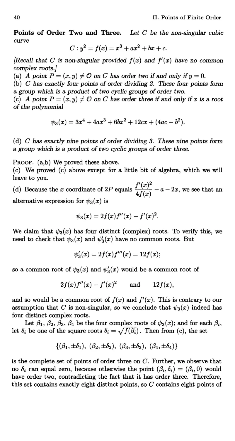
1. Points of Order Two and Three 38
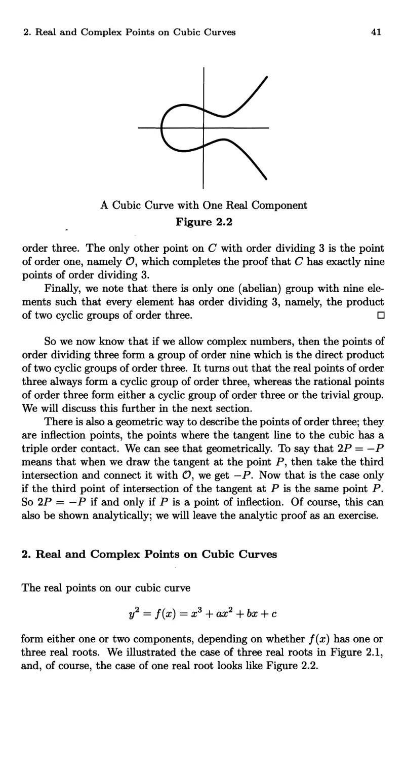
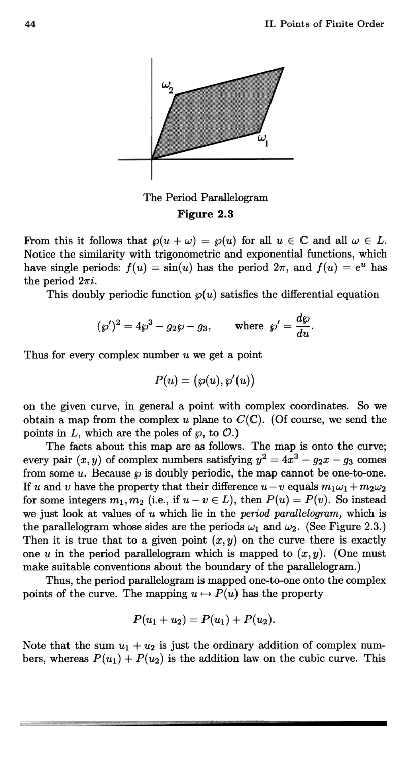
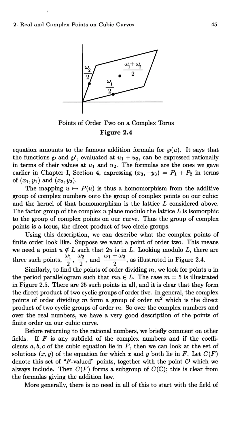
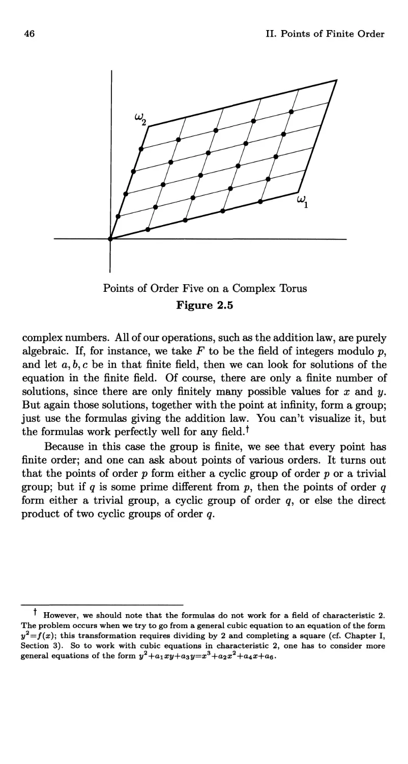
2. Real and Complex Points on Cubic Curves 41
3. The Discriminant 47
4. Points of Finite Order Have Integer Coordinates 49
5. The Nagell-Lutz Theorem and Further Developments 56
Exercises 58
CHAPTER HI
The Group of Rational Points 63
1. Heights and Descent 63
2. The Height of P + Po 68
3. The Height of 2P 71
4. A Useful Homomorphism 76
5. MordelPs Theorem 83
6. Examples and Further Developments 89
7. Singular Cubic Curves 99
Exercises 102
x Contents
CHAPTER IV
Cubic Curves over Finite Fields 107
1. Rational Points over Finite Fields 107
2. A Theorem of Gauss 110
3. Points of Finite Order Revisited 121
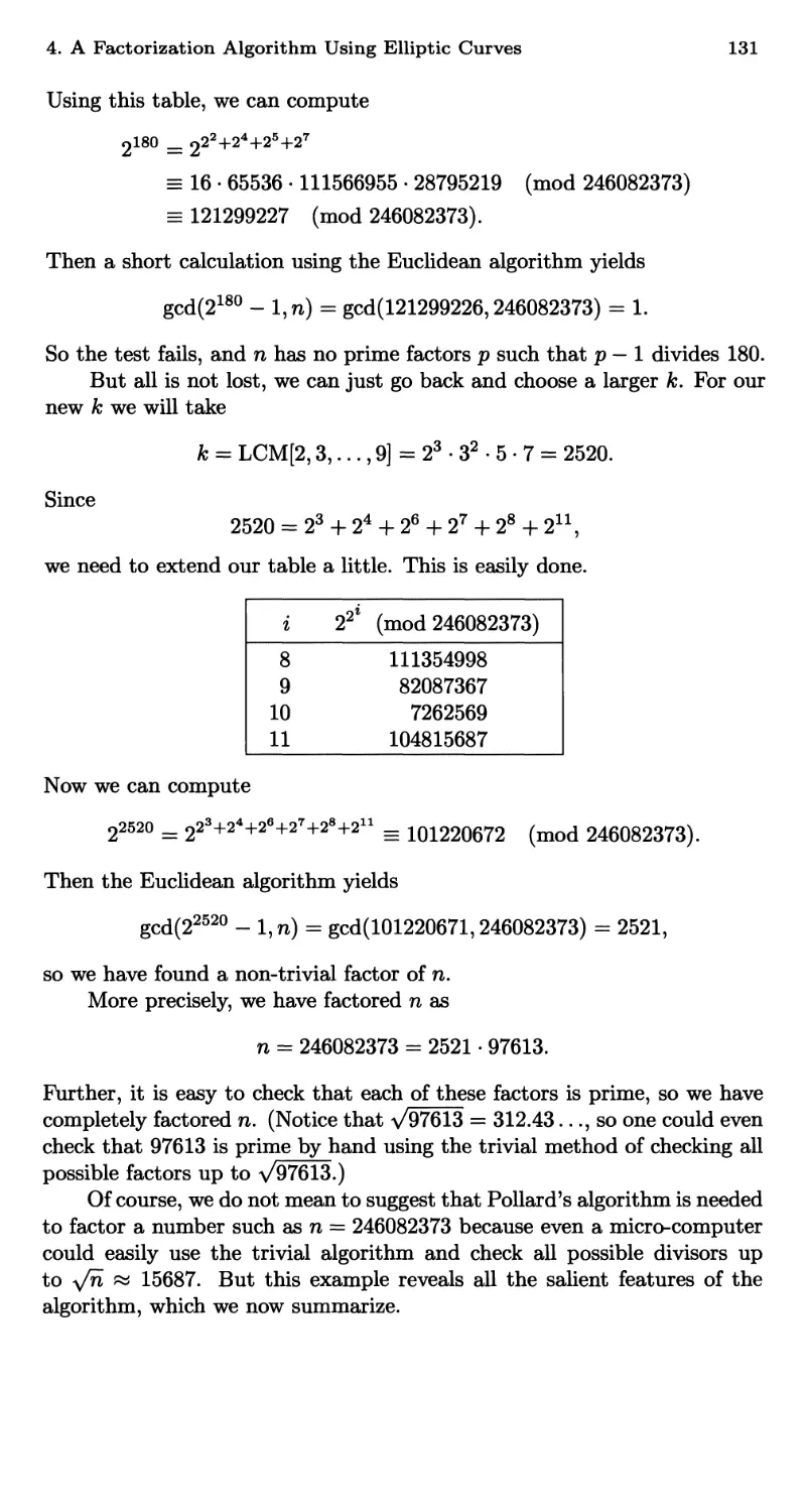
4. A Factorization Algorithm Using Elliptic Curves 125
Exercises 138
CHAPTER V
Integer Points on Cubic Curves 145
1. How Many Integer Points? 145
2. Taxicabs and Sums of Two Cubes 147
3. Thue's Theorem and Diophantine Approximation 152
4. Construction of an Auxiliary Polynomial 157
5. The Auxiliary Polynomial Is Small 165
6. The Auxiliary Polynomial Does Not Vanish 168
7. Proof of the Diophantine Approximation Theorem 171
8. Further Developments 174
Exercises 177
CHAPTER VI
Complex Multiplication 180
1. Abelian Extensions of Q 180
2. Algebraic Points on Cubic Curves 185
3. A Galois Representation 193
4. Complex Multiplication 199
5. Abelian Extensions of Q(i) 205
Exercises 213
APPENDIX A
Projective Geometry 220
1. Homogeneous Coordinates and the Projective Plane 220
2. Curves in the Projective Plane 225
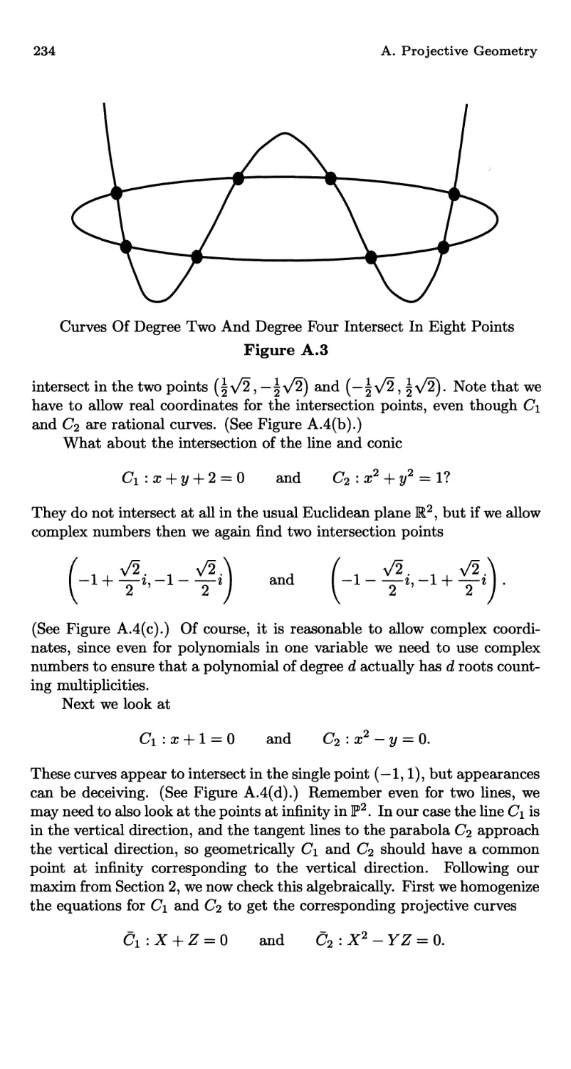
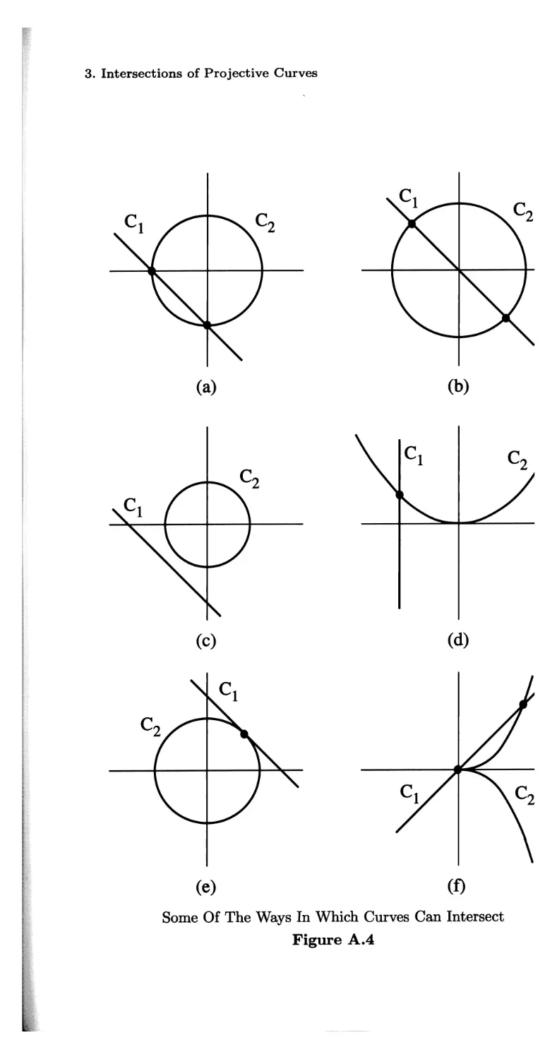
3. Intersections of Projective Curves 233
4. Intersection Multiplicities and a Proof of Bezout's Theorem 242
5. Reduction Modulo p 251
Exercises 254
Bibliography 259
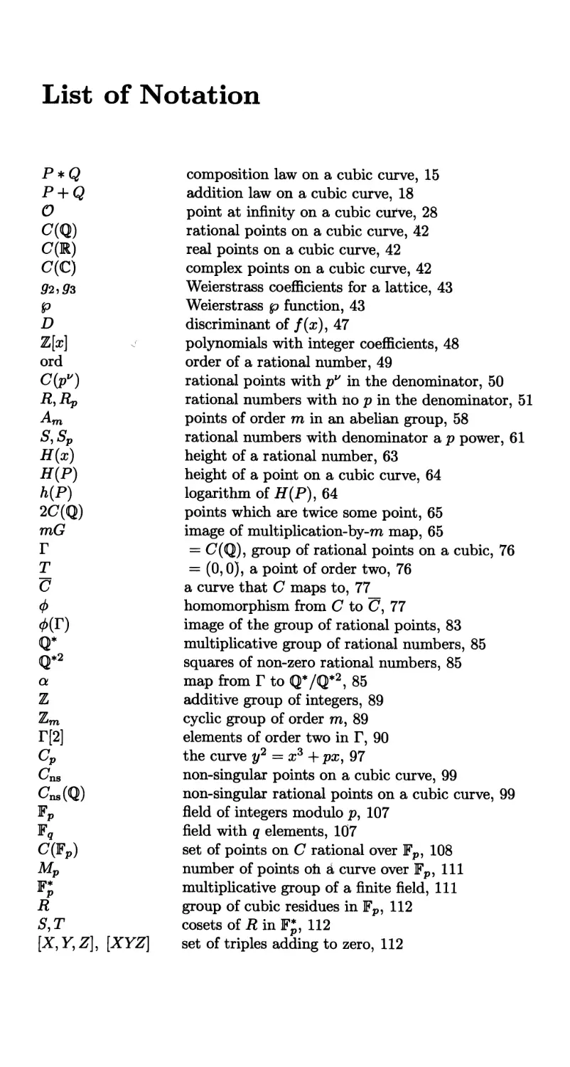
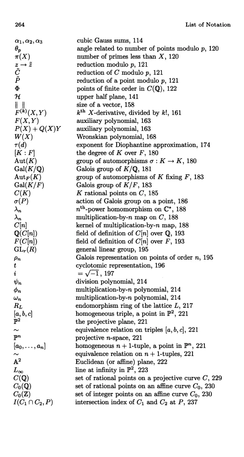
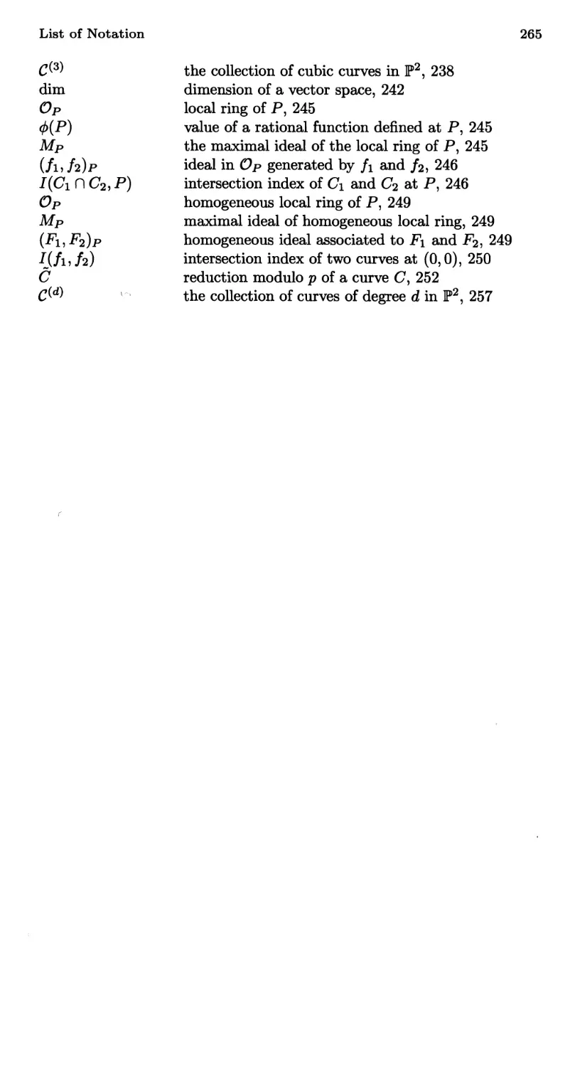
List of Notation 263
Index 267
Introduction
The theory of Diophantine equations is that branch of number theory which
deals with the solution of polynomial equations in either integers or rational
numbers. The subject itself is named after one of the greatest of the ancient
Greek algebraists, Diophantus of Alexandria,1 who formulated and solved
many such problems.
Most readers will undoubtedly be familiar with Fermat's Last Theo-
Theorem.2 This theorem says that if n > 3 is an integer, then the equation
Xn + Yn = Zn
has no solutions in non-zero integers X, Y, Z. Equivalently, the only solu-
solutions in rational numbers to the equation
xn + yn = 1
are those with either x = 0 or у = 0. Fermat's Theorem is now known to
be true for all exponents n < 125000, so it is unlikely that anyone will find
a counterexample by random guessing. On the other hand, there are still
a lot of possible exponents left to check between 125000 and infinity!
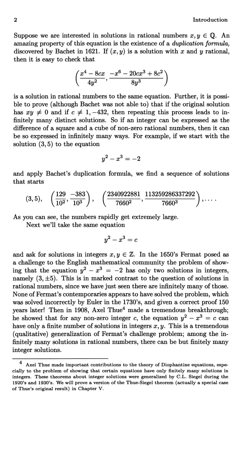
As another example, we consider the problem of writing an integer as
the difference of a square and a cube. In other words, we fix an integer с G Z
and look for solutions to the Diophantine equation3
Diophantus lived sometime before the 3rd century A.D. He wrote the Arithmetical a
treatise on algebra and number theory in 13 volumes, of which 6 volumes have survived.
2
Fermat's Last "Theorem" is really a conjecture, because it is still unsolved after more
than 350 years. Fermat stated his "Theorem" as a marginal note in his copy of Diophantus'
Arithmetical unfortunately, the margin was too small for him to write down his proof!
This equation is often called Bachet's equation, after the 17* century mathematician
who originally discovered the duplication formula. It is also sometimes called Mordell's equa-
equation, in honor of the 20th century mathematician L.J. Mordell, who made a fundamental
contribution to the solution of this and many similar Diophantine equations. We will be
proving a special case of Mordell's theorem in Chapter III.
2 Introduction
Suppose we are interested in solutions in rational numbers x, у € Q. An
amazing property of this equation is the existence of a duplication formula,
discovered by Bachet in 1621. If (ж, у) is a solution with x and у rational,
then it is easy to check that
x4 - 8cx -x6 - 20сж3 + 8c2 \
Ay2 ' Ъу3 )
is a solution in rational numbers to the same equation. Further, it is possi-
possible to prove (although Bachet was not able to) that if the original solution
has xy ф 0 and if с ф 1, —432, then repeating this process leads to in-
infinitely many distinct solutions. So if an integer can be expressed as the
difference of a square and a cube of non-zero rational numbers, then it can
be so expressed in infinitely many ways. For example, if we start with the
solution C,5) to the equation
?/2 - r3 - -2
and apply Bachet's duplication formula, we find a sequence of solutions
that starts
/129 -383 \ /2340922881 113259286337292 \
C'5)' VЮ2' Ю3 ) ' V 76602 ' 76603 )'""
As you can see, the numbers rapidly get extremely large.
Next we'll take the same equation
y*-x3=c
and ask for solutions in integers x,y € Z. In the 1650's Fermat posed as
a challenge to the English mathematical community the problem of show-
showing that the equation y2 — x3 = —2 has only two solutions in integers,
namely C, ±5). This is in marked contrast to the question of solutions in
rational numbers, since we have just seen there are infinitely many of those.
None of Fermat's contemporaries appears to have solved the problem, which
was solved incorrectly by Euler in the 1730's, and given a correct proof 150
years later! Then in 1908, Axel Thue4 made a tremendous breakthrough;
he showed that for any non-zero integer c, the equation y2 — x3 = с can
have only a finite number of solutions in integers x, y. This is a tremendous
(qualitative) generalization of Fermat's challenge problem; among the in-
infinitely many solutions in rational numbers, there can be but finitely many
integer solutions.
Axel Thue made important contributions to the theory of Diophantine equations, espe-
especially to the problem of showing that certain equations have only finitely many solutions in
integers. These theorems about integer solutions were generalized by C.L. Siegel during the
1920's and 1930's. We will prove a version of the Thue-Siegel theorem (actually a special case
of Thue's original result) in Chapter V.
Introduction
КО)
@,1)
A,0)
@,-1)
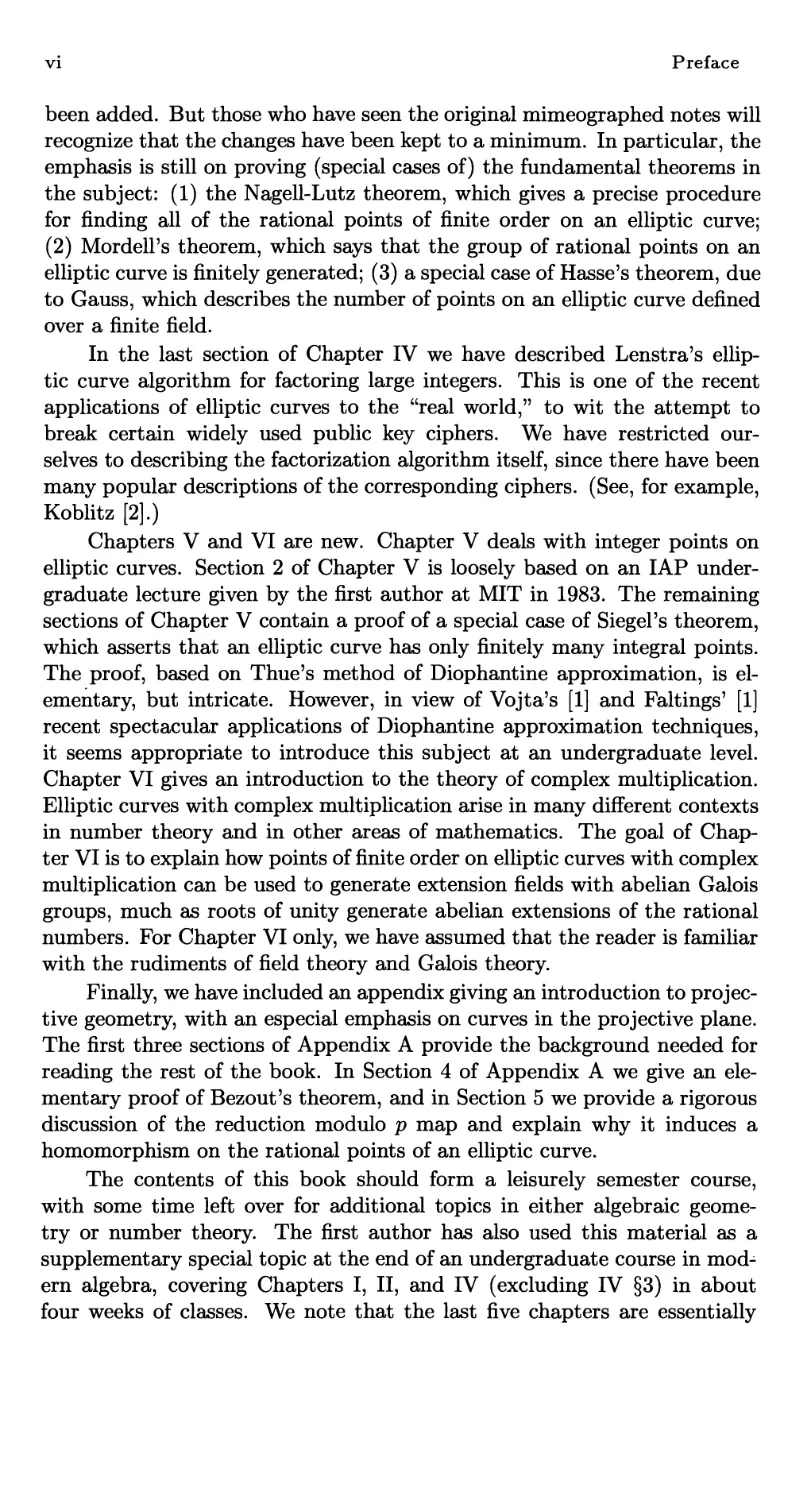
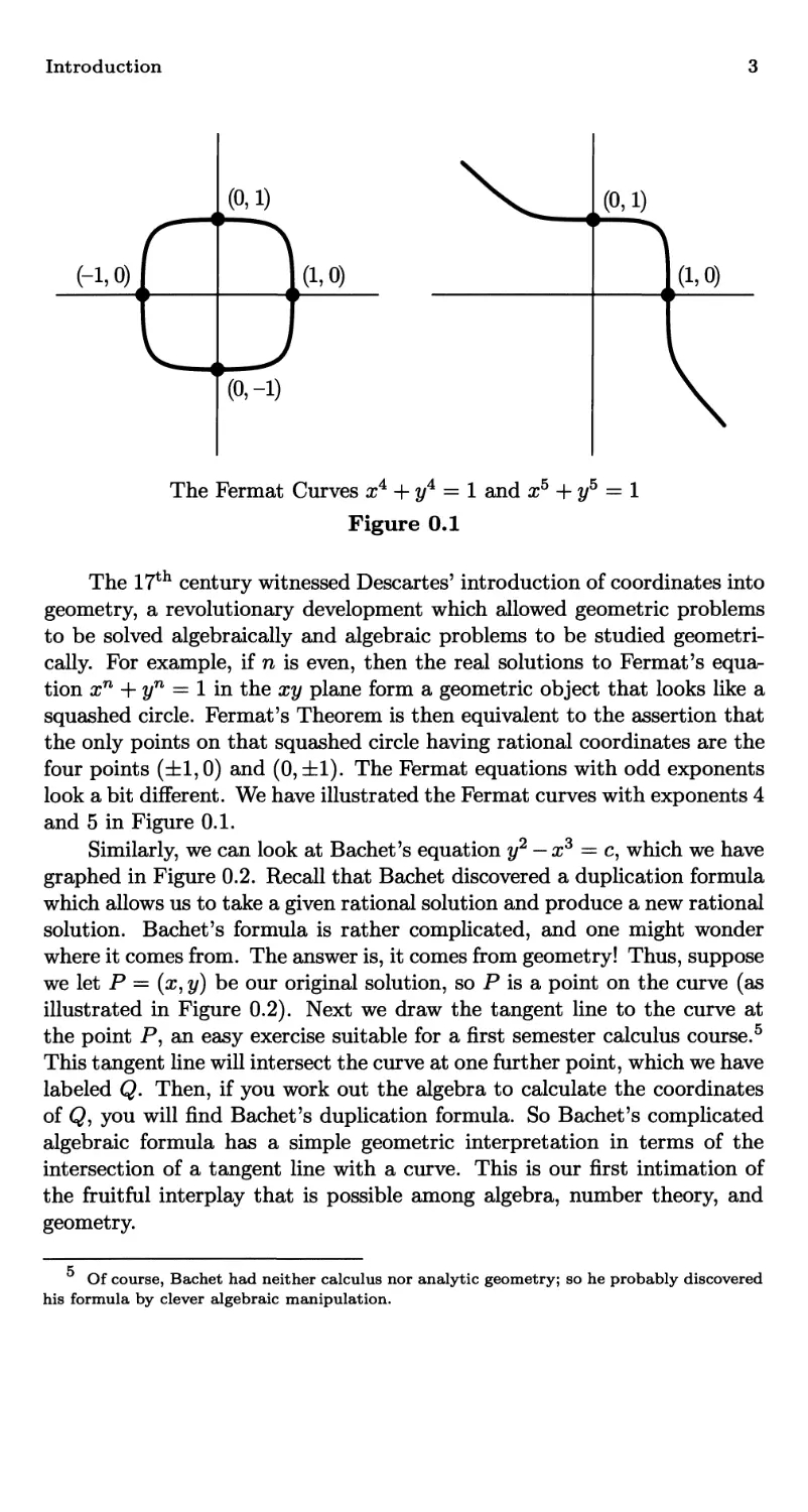
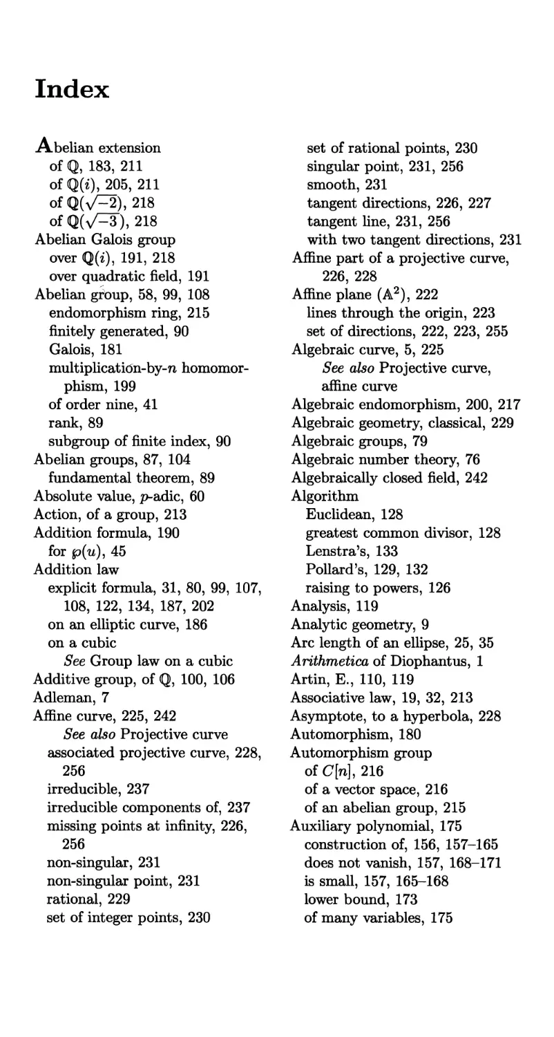
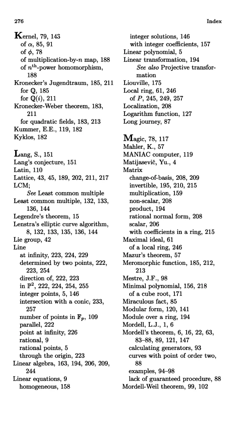
The Fermat Curves x4 + y4 = 1 and x5 + y5 = 1
Figure 0.1
The 17th century witnessed Descartes' introduction of coordinates into
geometry, a revolutionary development which allowed geometric problems
to be solved algebraically and algebraic problems to be studied geometri-
geometrically. For example, if n is even, then the real solutions to Fermat's equa-
equation xn + yn = 1 in the xy plane form a geometric object that looks like a
squashed circle. Fermat's Theorem is then equivalent to the assertion that
the only points on that squashed circle having rational coordinates are the
four points (±1,0) and @, ±1). The Fermat equations with odd exponents
look a bit different. We have illustrated the Fermat curves with exponents 4
and 5 in Figure 0.1.
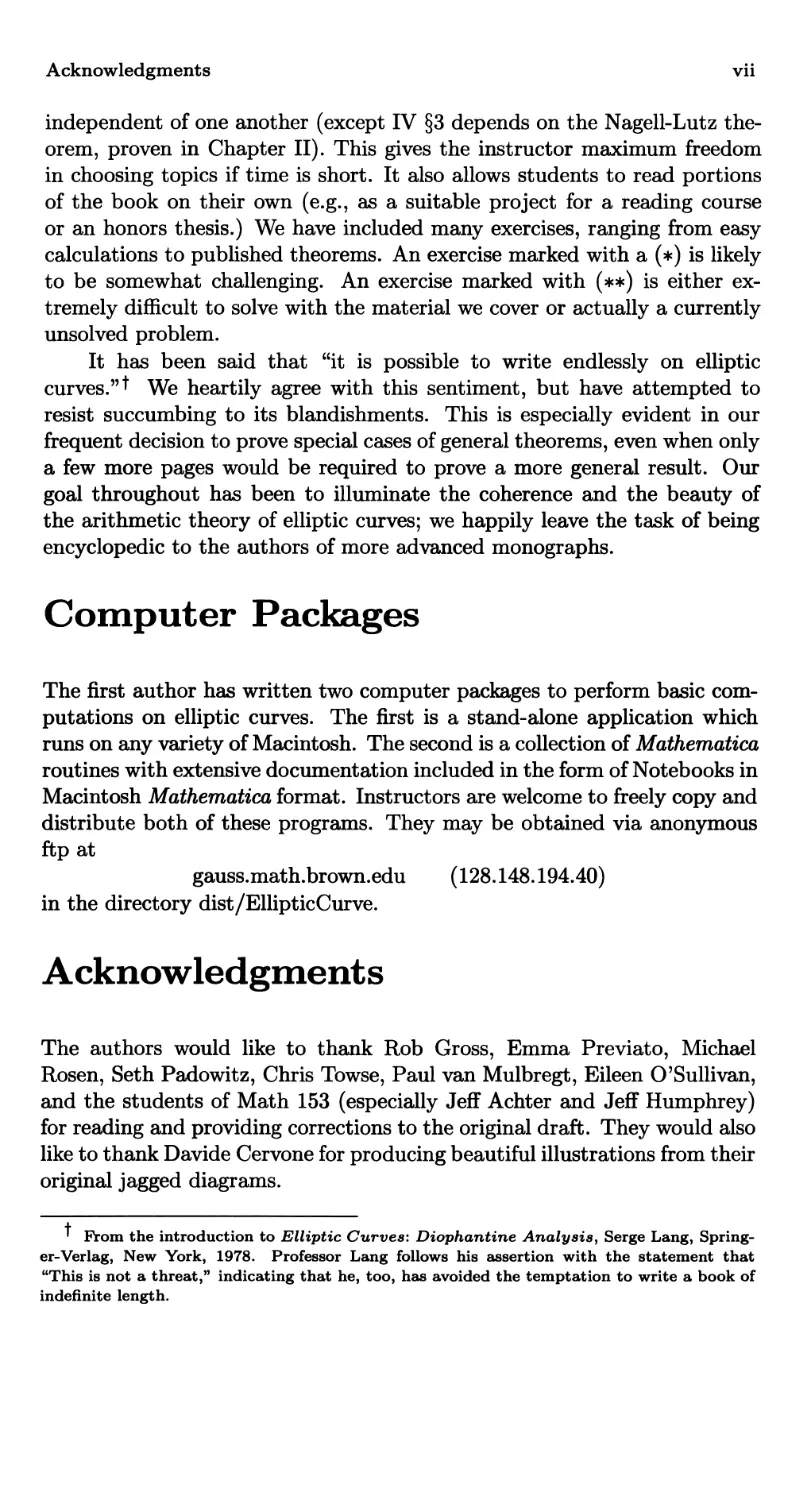
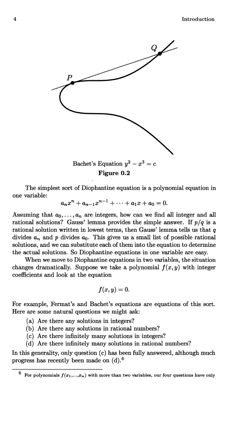
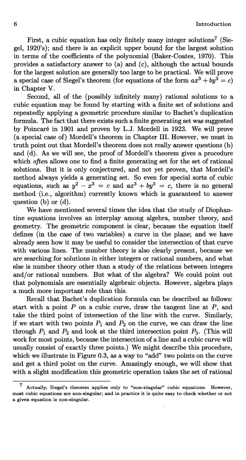
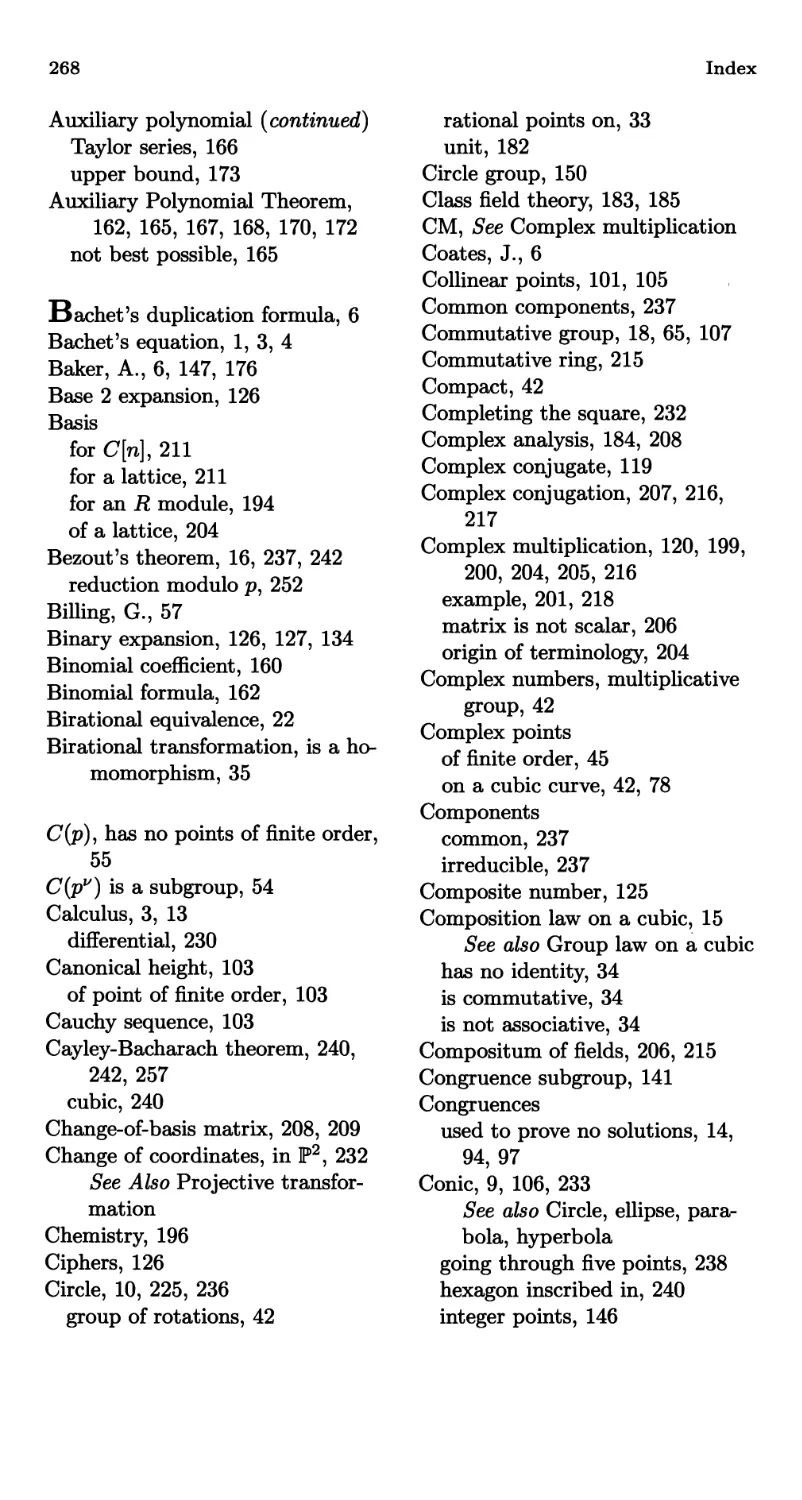
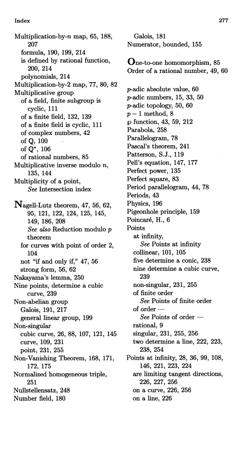
Similarly, we can look at Bachet's equation y2 — x3 = c, which we have
graphed in Figure 0.2. Recall that Bachet discovered a duplication formula
which allows us to take a given rational solution and produce a new rational
solution. Bachet's formula is rather complicated, and one might wonder
where it comes from. The answer is, it comes from geometry! Thus, suppose
we let P = (x, y) be our original solution, so P is a point on the curve (as
illustrated in Figure 0.2). Next we draw the tangent line to the curve at
the point P, an easy exercise suitable for a first semester calculus course.5
This tangent line will intersect the curve at one further point, which we have
labeled Q. Then, if you work out the algebra to calculate the coordinates
of Q, you will find Bachet's duplication formula. So Bachet's complicated
algebraic formula has a simple geometric interpretation in terms of the
intersection of a tangent line with a curve. This is our first intimation of
the fruitful interplay that is possible among algebra, number theory, and
geometry.
Of course, Bachet had neither calculus nor analytic geometry; so he probably discovered
his formula by clever algebraic manipulation.
Introduction
Q
Bachet's Equation y2 — x3 = с
Figure 0.2
The simplest sort of Diophantine equation is a polynomial equation in
one variable:
anxn + dn-xx"-1 + • • • + агх + a0 = 0.
Assuming that ao,..., сьп are integers, how can we find all integer and all
rational solutions? Gauss' lemma provides the simple answer. If p/q is a
rational solution written in lowest terms, then Gauss' lemma tells us that q
divides an and p divides ao. This gives us a small list of possible rational
solutions, and we can substitute each of them into the equation to determine
the actual solutions. So Diophantine equations in one variable are easy.
When we move to Diophantine equations in two variables, the situation
changes dramatically. Suppose we take a polynomial f(x,y) with integer
coefficients and look at the equation
f(x,y) = 0.
For example, Fermat's and Bachet's equations are equations of this sort.
Here are some natural questions we might ask:
(a) Are there any solutions in integers?
(b) Are there any solutions in rational numbers?
(c) Are there infinitely many solutions in integers?
(d) Are there infinitely many solutions in rational numbers?
In this generality, only question (c) has been fully answered, although much
progress has recently been made on (d).6
For polynomials f(xi,...,xn) with more than two variables, our four questions have only
Introduction 5
The set of real solutions to an equation f(x,y) = 0 forms a curve
in the xy plane. Such curves are often called algebraic curves to indicate
that they are the solutions of a polynomial equation. In trying to answer
questions (a)-(d), we might begin by looking at simple polynomials, such
as polynomials of degree 1 (also called linear polynomials, because their
graphs are straight lines.) For a linear equation
ax + by = с
with integer coefficients, it is easy to answer our questions. There are always
infinitely many rational solutions, there are no integer solutions if gcd(a, b)
does not divide c, and otherwise there are infinitely many integer solutions.
So linear equations are even easier than equations in one variable.
Next we might turn to polynomials of degree 2 (also called quadratic
polynomials). Their graphs are conic sections. It turns out that if such
ал equation has one rational solution, then there are infinitely many. The
complete set of solutions can be described very easily using geometry. We
will explain how this is done in the first section of Chapter I. We will also
briefly indicate how to answer question (b) for quadratic polynomials. So
although it would be untrue to say that quadratic polynomials are easy, it
is fair to say that their solutions are completely understood.
This brings us to the main topic of this book, namely, the solution of
degree 3 polynomial equations in rational numbers and in integers. One
example of such an equation is Bachet's equation y2 — x3 = с which we
looked at earlier; some other examples which will appear during our studies
are
y2 = x3 + ax2 + bx + c and ax3 -\-by3 = с
The real solutions to these equations are called cubic curves or elliptic
curves. (However, they are not ellipses, since ellipses are conic sections,
and conic sections are given by quadratic equations! The curious chain
of events that led to elliptic curves being so named will be recounted in
Chapter I, Section 3.) In contrast to linear and quadratic equations, the
rational and integer solutions to cubic equations are still not completely
understood; and even in those cases where the complete answers are known,
the proofs involve a subtle blend of techniques from algebra, number theory,
and geometry. Our main goal in this book is to introduce you to the
beautiful subject of Diophantine equations by studying in depth the first
case of such equations which are still imperfectly understood, namely cubic
equations in two variables. To give you an idea of the sorts of results we
will be studying, we briefly indicate what is known about questions (a)-(d).
been answered for some very special sorts of equations. Even worse, work of Davis, Matijasevic,
and Robinson has shown that in general it is not possible to find a solution to question (a).
That is, there does not exist an algorithm which takes as input the polynomial / and produces
as output either "YES" or "NO" as an answer to question (a).
6 Introduction
First, a cubic equation has only finitely many integer solutions7 (Sie-
gel, 1920's); and there is an explicit upper bound for the largest solution
in terms of the coefficients of the polynomial (Baker-Coates, 1970). This
provides a satisfactory answer to (a) and (c), although the actual bounds
for the largest solution are generally too large to be practical. We will prove
a special case of SiegeFs theorem (for equations of the form ax3 + by3 = c)
in Chapter V.
Second, all of the (possibly infinitely many) rational solutions to a
cubic equation may be found by starting with a finite set of solutions and
repeatedly applying a geometric procedure similar to Bachet's duplication
formula. The fact that there exists such a finite generating set was suggested
by Poincare in 1901 and proven by L.J. Mordell in 1923. We will prove
(a special case of) Mordell's theorem in Chapter III. However, we must in
truth point out that Mordell's theorem does not really answer questions (b)
and (d). As we will see, the proof of Mordell's theorem gives a procedure
which often allows one to find a finite generating set for the set of rational
solutions. But it is only conjectured, and not yet proven, that Mordell's
method always yields a generating set. So even for special sorts of cubic
equations, such as y2 — x3 = с and ax3 + by3 = c, there is no general
method (i.e., algorithm) currently known which is guaranteed to answer
question (b) or (d).
We have mentioned several times the idea that the study of Diophan-
tine equations involves an interplay among algebra, number theory, and
geometry. The geometric component is clear, because the equation itself
defines (in the case of two variables) a curve in the plane; and we have
already seen how it may be useful to consider the intersection of that curve
with various lines. The number theory is also clearly present, because we
are searching for solutions in either integers or rational numbers, and what
else is number theory other than a study of the relations between integers
and/or rational numbers. But what of the algebra? We could point out
that polynomials are essentially algebraic objects. However, algebra plays
a much more important role than this.
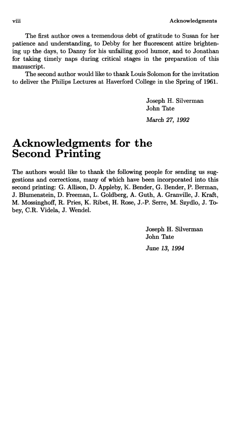
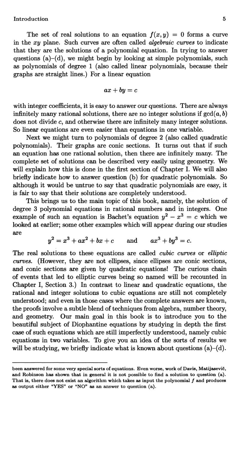
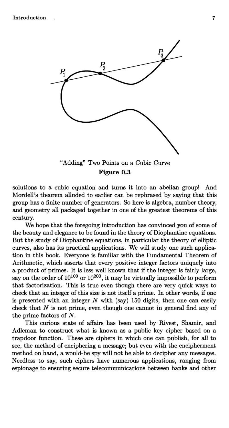
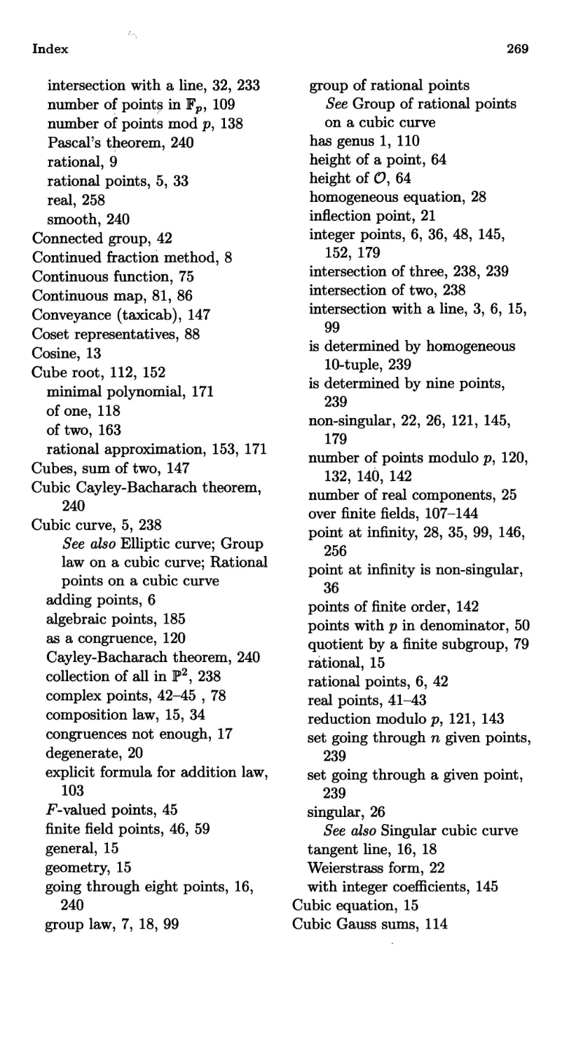
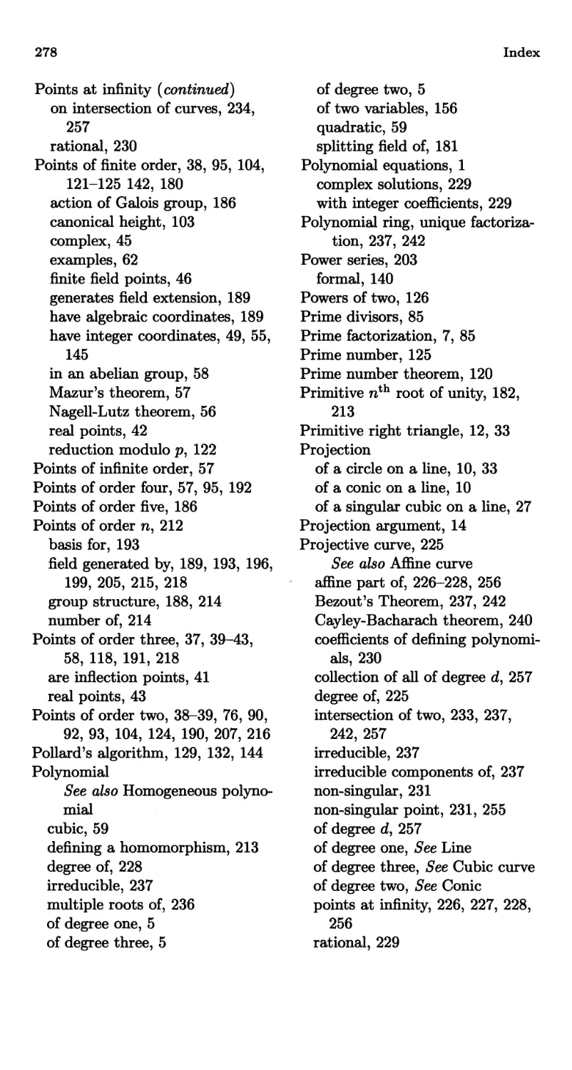
Recall that Bachet's duplication formula can be described as follows:
start with a point P on a cubic curve, draw the tangent line at P, and
take the third point of intersection of the line with the curve. Similarly,
if we start with two points Pi and P^ on the curve, we can draw the line
through P\ and P^ and look at the third intersection point P3. (This will
work for most points, because the intersection of a line and a cubic curve will
usually consist of exactly three points.) We might describe this procedure,
which we illustrate in Figure 0.3, as a way to "add" two points on the curve
and get a third point on the curve. Amazingly enough, we will show that
with a slight modification this geometric operation takes the set of rational
ГУ
Actually, Siegel's theorem applies only to "non-singular" cubic equations. However,
most cubic equations are non-singular; and in practice it is quite easy to check whether or not
a given equation is non-singular.
Introduction
"Adding" Two Points on a Cubic Curve
Figure 0.3
solutions to a cubic equation and turns it into an abelian group! And
Mordell's theorem alluded to earlier can be rephrased by saying that this
group has a finite number of generators. So here is algebra, number theory,
and geometry all packaged together in one of the greatest theorems of this
century.
We hope that the foregoing introduction has convinced you of some of
the beauty and elegance to be found in the theory of Diophantine equations.
But the study of Diophantine equations, in particular the theory of elliptic
curves, also has its practical applications. We will study one such applica-
application in this book. Everyone is familiar with the Fundamental Theorem of
Arithmetic, which asserts that every positive integer factors uniquely into
a product of primes. It is less well known that if the integer is fairly large,
say on the order of 10100 or 10200, it may be virtually impossible to perform
that factorization. This is true even though there are very quick ways to
check that an integer of this size is not itself a prime. In other words, if one
is presented with an integer N with (say) 150 digits, then one can easily
check that N is not prime, even though one cannot in general find any of
the prime factors of N.
This curious state of affairs has been used by Rivest, Shamir, and
Adleman to construct what is known as a public key cipher based on a
trapdoor function. These are ciphers in which one can publish, for all to
see, the method of enciphering a message; but even with the encipherment
method on hand, a would-be spy will not be able to decipher any messages.
Needless to say, such ciphers have numerous applications, ranging from
espionage to ensuring secure telecommunications between banks and other
8 Introduction
financial institutions. To describe the relation with elliptic curves, we will
need to briefly indicate how such a "trapdoor cipher" works.
First one chooses two large primes, say p and q, each with around 100
digits. Next one publishes the product N = pq. In order to encipher
a message, your correspondent only needs to know the value of N. But
in order to decipher a message, the factors p and q are needed. So your
messages will be safe as long as no one is able to factor N. This means
that in order to ensure the safety of your messages, you need to know the
largest integers that your enemies are able to factor in a reasonable amount
of time.
So how does one factor a large number which is known to be composite?
One can start trying possible divisors 2, 3,..., but this is hopelessly ineffi-
inefficient. Using techniques from number theory, various algorithms have been
devised, with exotic sounding names like the continued fraction method,
the ideal class group method, the p — 1 method, and the quadratic sieve
method. But one of the best methods currently available is Lenstra's El-
Elliptic Curve Algorithm, which as the name indicates relies on the theory
of elliptic curves. So it is essential to understand the strength of Lenstra's
algorithm if one is to ensure that one's public key cipher will not be broken.
We will describe how Lenstra's algorithm works in Chapter IV.
CHAPTER I
Geometry and Arithmetic
1. Rational Points on Conies
Everyone knows what a rational number is, a quotient of two integers. We
call a point in the (ж, у) plane a rational point if both its coordinates are
rational numbers. We call a line a rational line if the equation of the line
can be written with rational numbers; that is, if its equation is
ax + by + с = О
with a, 6, c, rational. Now it is pretty obvious that if you have two rational
points, the line through them is a rational line. And it is neither hard to
guess nor hard to prove that if you have two rational lines, then the point
where they intersect is a rational point. If you have two linear equations
with rational numbers as coefficients and you solve them, you get rational
numbers as answers.
The general subject of these notes is rational points on curves, espe-
especially on cubic curves. But as an introduction, we will start with conies.
Let
ax2 + bxy + cy2 + dx + ey + / = 0
be a conic. We will say that the conic is rational if we can write its equation
with rational numbers.
Now what about the intersection of a rational line with a rational conic?
Will it be true that the points of intersection are rational. By writing down
some examples, it is easy to see that the answer is, in general, no. If you use
analytic geometry to find the coordinates of these points, you will come out
with a quadratic equation for the x coordinate of the intersection. And if the
conic is rational and the line is rational, the quadratic equation you come
out with will have rational coefficients. So the two points of intersection will
be rational if and only if the roots of that quadratic equation are rational.
In general, they might be conjugate quadratic irrationalities.
However, if one of those points is rational, then so is the other. This
is true because if a quadratic equation with rational coefficients has one
10 I. Geometry and Arithmetic
Projecting a Conic onto a Line
Figure 1.1
rational root, then the other root is rational, because the sum of the roots
is the middle coefficient. This very simple idea enables one to describe
the rational points on a conic completely. Given a rational conic, the first
question is whether or not there are any rational points on it. (We will
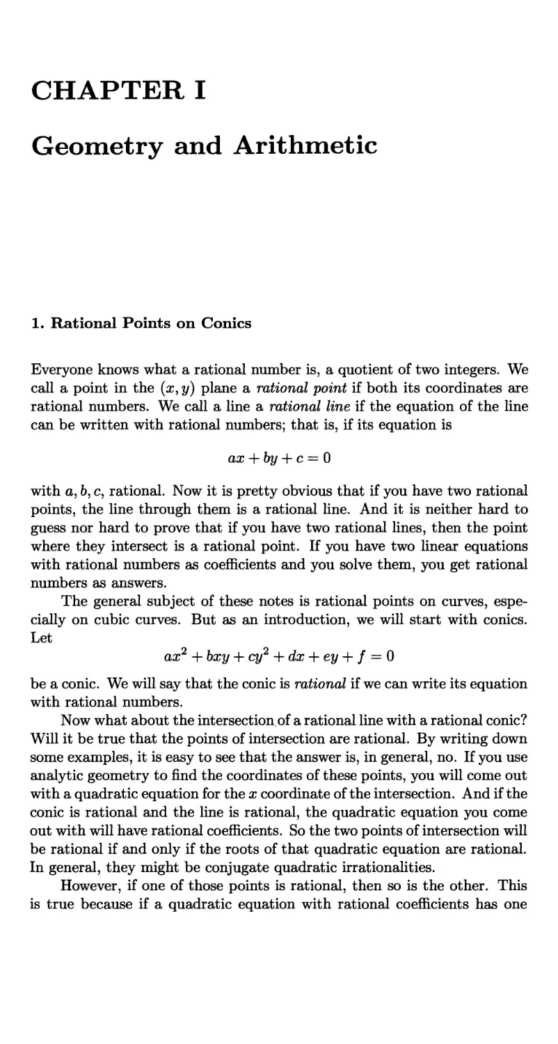
return to this question later.) But let us suppose that we know of one
rational point О on our rational conic. Then we can get all of them very
simply. We just draw some rational line and we project the conic onto the
line from this point O. (To project О itself onto the line, we use the tangent
line to the conic at O.)
A line meets a conic in two points, so for every point P on the conic we
get a point Q on the line; and conversely, for every point Q on the line, by
joining it to the point 0, we get a point P on the conic. (See Figure 1.1.)
We get a one-to-one correspondence between the points on the conic and
points on the line.t But now you see by the remarks we have made that if
the point P on the conic has rational coordinates, then the point Q on the
line will have rational coordinates. And conversely, if Q is rational, then
because О is assumed to be rational, the line through P and Q meets the
conic in two points, one of which is rational. So the other point is rational,
too. Thus the rational points on the conic are in one-to-one correspondence
with the rational points on the line. Of course, the rational points on the
line are easily described in terms of rational values of some parameter.
Let's carry out this procedure for the circle
x2+y2 = l.
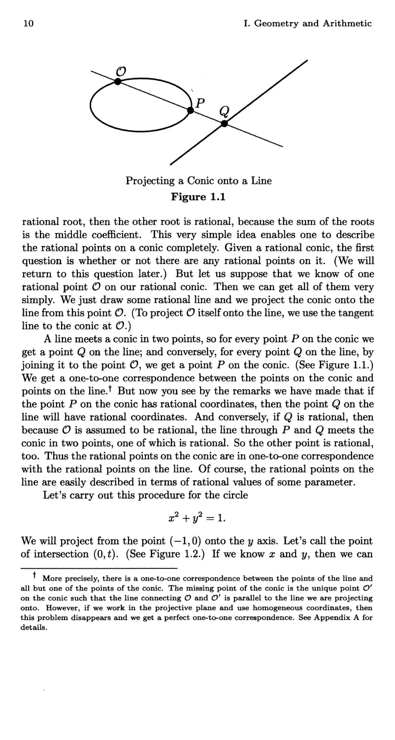
We will project from the point (—1,0) onto the у axis. Let's call the point
of intersection @,£). (See Figure 1.2.) If we know x and y, then we can
T More precisely, there is a one-to-one correspondence between the points of the line and
all but one of the points of the conic. The missing point of the conic is the unique point O'
on the conic such that the line connecting О and O' is parallel to the line we are projecting
onto. However, if we work in the projective plane and use homogeneous coordinates, then
this problem disappears and we get a perfect one-to-one correspondence. See Appendix A for
details.
1. Rational Points on Conies
11
A Rational Parametrization of the Circle
Figure 1.2
get t very easily. The equation of the line L connecting (—1,0) to @, t)
is у = t(l + x). The point (ж, у) is assumed to be on the line L and also on
the circle, so we get the relation
l-x2=y2=t2(l + xJ.
For a fixed value of t, this is a quadratic equation whose roots are the x
coordinates of the two intersections of the line L with the circle. Clearly, x =
— 1 is a root, because the point (—1,0) is on both L and the circle. To find
the other root, we cancel a factor of 1 + x from both sides of the equation.
This gives the linear equation 1 — x = t2(l + x). Solving this for x in terms
of t, and then using the relation у = t(l + x) to find y, we obtain
1-t2
X =
У =
2t
+2'
This is the familiar rational parametrization of the circle . And now
the assertion made above is clear from these formulas. That is, if x and у
are rational numbers, then t will be a rational number. Conversely, if t is
a rational number, then from these formulas it is obvious that the coordi-
coordinates x and у will be rational numbers. So this is the way you get rational
points on the circle: simply plug in an arbitrary rational number for t. That
will give you all points except (—1,0). [If you want to get (—1,0), you must
"substitute" infinity for t\]
These formulas can be used to solve the elementary problem of de-
describing all right triangles with integer sides. Let us consider the problem
of finding some other triangles, besides 3,4,5, which have whole number
12
I. Geometry and Arithmetic
Y
X
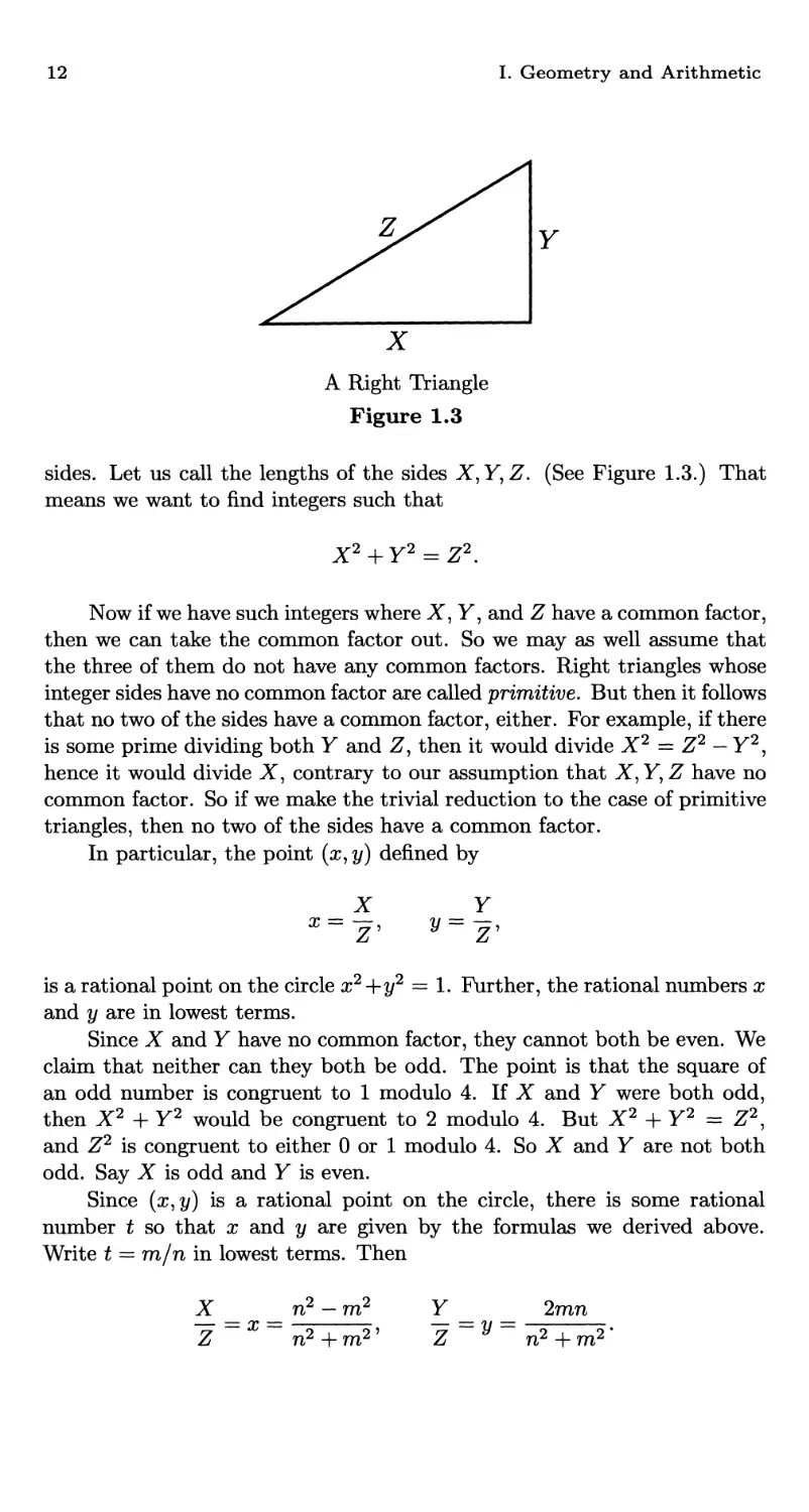
A Right Triangle
Figure 1.3
sides. Let us call the lengths of the sides X,Y,Z. (See Figure 1.3.) That
means we want to find integers such that
Now if we have such integers where X, Y, and Z have a common factor,
then we can take the common factor out. So we may as well assume that
the three of them do not have any common factors. Right triangles whose
integer sides have no common factor are called primitive. But then it follows
that no two of the sides have a common factor, either. For example, if there
is some prime dividing both Y and Z, then it would divide X2 = Z2 — Y2,
hence it would divide X, contrary to our assumption that X, Y, Z have no
common factor. So if we make the trivial reduction to the case of primitive
triangles, then no two of the sides have a common factor.
In particular, the point (x, y) defined by
x =
X
z'
Y
is a rational point on the circle x2 +y2 = 1. Further, the rational numbers x
and у are in lowest terms.
Since X and Y have no common factor, they cannot both be even. We
claim that neither can they both be odd. The point is that the square of
an odd number is congruent to 1 modulo 4. If X and Y were both odd,
then X2 + Y2 would be congruent to 2 modulo 4. But X2 + Y2 = Z2,
and Z2 is congruent to either 0 or 1 modulo 4. So X and Y are not both
odd. Say X is odd and Y is even.
Since (x,y) is a rational point on the circle, there is some rational
number t so that x and у are given by the formulas we derived above.
Write t = m/n in lowest terms. Then
n2-m2
Y
2mn
n2 + m2
1. Rational Points on Conies 13
Since X/Z and Y/Z are in lowest terms, this means that there is some
integer A so that
XZ = n2 + m2, XY = 2mn, AX = n2 — m2.
We want to show that A = 1. Because A divides both n2+m2 and n2 —
m2, it divides their sum 2n2 and their difference 2m2. But m and n have
no common divisors. Hence, A divides 2, and so A = 1 or A = 2. If A = 2,
then n2 — m2 = XX is divisible by 2, but not by 4, because we are assuming
that X is odd. In other words, n2 — m2 is congruent to 2 modulo 4. But n2
and m2 are each congruent to either 0 or 1 modulo 4, so this is not possible.
Hence, A = 1.
This proves that to get all primitive triangles, you take two relatively
prime integers m and n and let
be the sides of the triangle. These are the ones with X odd and Y even.
The others are obtained by interchanging X and Y.
These formulas have other uses; you may have met them in calculus .
In Figure 1.2, we have
x = cos#, у = sin#; and so t = tan hO = -.
1 + cos в
So the formulas given above allow us to express cosine and sine rationally
in terms of the tangent of the half angle:
.. I-*2 . л 2t
x = <
If you have some complicated identity in sine and cosine that you want
to test, all you have to do is substitute these formulas, collect powers of £,
and see if you get zero. (If they had told you this in high school, the whole
business of trigonometric identities would have become a trivial exercise in
algebra!)
Another use comes from the observation that these formulas let us
express all trigonometric functions of an angle в as rational expressions
in t = tan@/2). Note that
Oil
в = 2 arctan(t), d9 =
It*
So if you have an integral which involves cos в and sin в and dO, and you
make the appropriate substitutions, then you transform it into an integral
in t and dt. If the integral is a rational function of sin# and cos#, you
obviously come out with the integral of a rational function of t. Since
rational functions can be integrated in terms of elementary functions, it
14 I. Geometry and Arithmetic
follows that any rational function of sin в and cos 9 can be integrated in
terms of elementary functions.
What if we take the circle
and ask to find the rational points on it? That is the easiest problem of all,
because the answer is that there are none. It is impossible for the sum of
the squares of two rational numbers to equal 3. How can we see that it is
impossible?
If there is a rational point, we can write it as
X Y
x = — and у = —
for some integers X, Y, Z\ and then
If X, У, Z have a common factor, then we can remove it; so we may assume
that they have no common factor. It follows that both X and Y are not
divisible by 3. This is true because if 3 divides X, then 3 divides Y2 =
3Z2-X2, so 3 divides Y. But then 9 divides X2+Y2 = 3Z2, so 3 divides Z,
contradicting the fact that X, Y, Z have no common factors. Hence 3 does
not divide X, and similarly for Y.
Since X and Y are not divisible by 3, we have
X = ±l(mod3), r = ±l(mod3), and so X2 = Y2 = 1 (mod 3).
But then
0 = SZ2 = X2 + Y2 = 1 + 1 = 2 (mod 3).
This contradiction shows that no two rational numbers have squares which
add up to 3.
We have seen by the projection argument that if you have one rational
point on a rational conic, then all of the rational points can be described
in terms of a rational parameter t. But how do you check whether or not
there is one rational point? The argument we gave for x2 + y2 = 3 gives
the clue. We showed that there were no rational points by checking that a
certain equation had no solutions modulo 3.
There is a general method to test, in a finite number of steps, whether
or not a given rational conic has a rational point. The method consists in
seeing whether a certain congruence can be satisfied. The theorem goes
back to Legendre. Let us take the simple case
2. The Geometry of Cubic Curves 15
which is to be solved in integers. Legendre's theorem states that there is
an integer m, depending in a simple fashion on a, b, and c, so that the
above equation has a solution in integers, not all zero, if and only if the
congruence
aX2 + bY2 = cZ2 (mod m)
has a solution in integers relatively prime to m.
There is a much more elegant way to state this theorem, due to Hasse:
"A homogeneous quadratic equation in several variables is solvable by inte-
integers, not all zero, if and only if it is solvable in real numbers and in p-adic
numbers for each prime p." Once one has Hasse's result, then one gets
Legendre's theorem in a fairly elementary way. Legendre's theorem com-
combined with the work we did earlier provides a very satisfactory answer to
the question of rational points on rational conies. So now we move on to
cubics.
2. The Geometry of Cubic Curves
Now we are ready to begin our study of cubics. Let
ax3 + bx2y + cxy2 + dy3 + ex2 + fxy + gy2 + hx + iy + j = 0
be the equation for a general cubic. We will say that a cubic is rational if
the coefficients of its equation are rational numbers. A famous example is
or, in homogeneous form,
To find rational solutions of x3-\-y3 = 1 amounts to finding integer solutions
of X3 + У3 = Z3, the first non-trivial case of Fermat's Last "Theorem."
We cannot use the geometric principle that worked so well for conies
because a line generally meets a cubic in three points. And if we have one
rational point, we cannot project the cubic onto a line, because each point
on the line would then correspond to two points on the curve.
But there is a geometric principle we can use. If we can find two
rational points on the curve, then we can generally find a third one. Namely,
draw the line connecting the two points you have found. This will be a
rational line, and it meets the cubic in one more point. If we look and see
what happens when we try to find the three intersections of a rational line
with a rational cubic, we find that we come out with a cubic equation with
rational coefficients. If two of the roots are rational, then the third must
be also. We will work out some explicit examples below, but the principle
is clear. So this gives some kind of composition law: Starting with two
points P and Q, we draw the line through P and Q and let P * Q denote
the third point of intersection of the line with the cubic. (See Figure 1.4.)
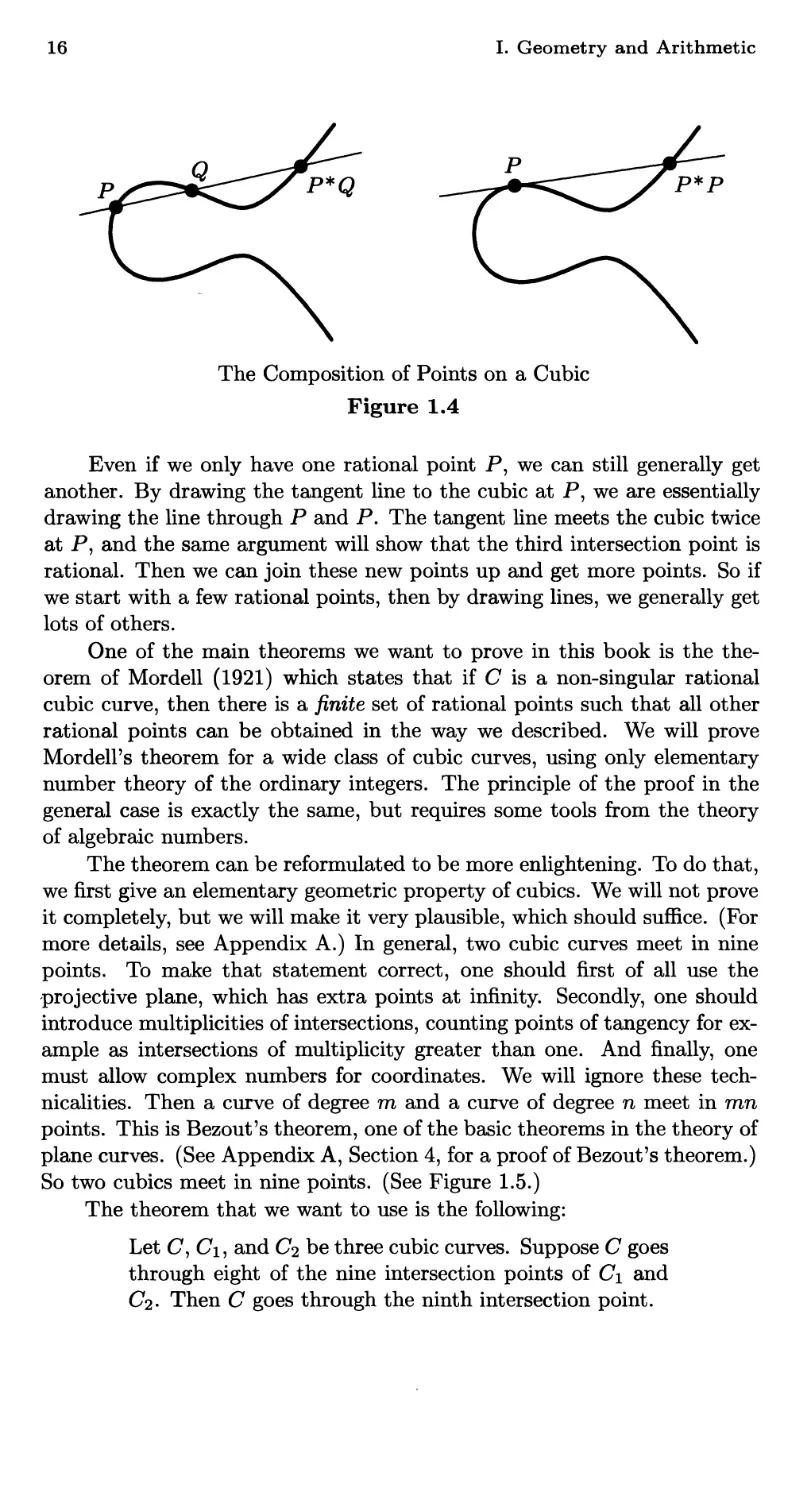
16 I. Geometry and Arithmetic
The Composition of Points on a Cubic
Figure 1.4
Even if we only have one rational point P, we can still generally get
another. By drawing the tangent line to the cubic at P, we are essentially
drawing the line through P and P. The tangent line meets the cubic twice
at P, and the same argument will show that the third intersection point is
rational. Then we can join these new points up and get more points. So if
we start with a few rational points, then by drawing lines, we generally get
lots of others.
One of the main theorems we want to prove in this book is the the-
theorem of Mordell A921) which states that if С is a non-singular rational
cubic curve, then there is a finite set of rational points such that all other
rational points can be obtained in the way we described. We will prove
Mordell's theorem for a wide class of cubic curves, using only elementary
number theory of the ordinary integers. The principle of the proof in the
general case is exactly the same, but requires some tools from the theory
of algebraic numbers.
The theorem can be reformulated to be more enlightening. To do that,
we first give an elementary geometric property of cubics. We will not prove
it completely, but we will make it very plausible, which should suffice. (For
more details, see Appendix A.) In general, two cubic curves meet in nine
points. To make that statement correct, one should first of all use the
projective plane, which has extra points at infinity. Secondly, one should
introduce multiplicities of intersections, counting points of tangency for ex-
example as intersections of multiplicity greater than one. And finally, one
must allow complex numbers for coordinates. We will ignore these tech-
technicalities. Then a curve of degree m and a curve of degree n meet in mn
points. This is Bezout's theorem, one of the basic theorems in the theory of
plane curves. (See Appendix A, Section 4, for a proof of Bezout's theorem.)
So two cubics meet in nine points. (See Figure 1.5.)
The theorem that we want to use is the following:
Let C, Ci, and C2 be three cubic curves. Suppose С goes
through eight of the nine intersection points of C\ and
C2. Then С goes through the ninth intersection point.
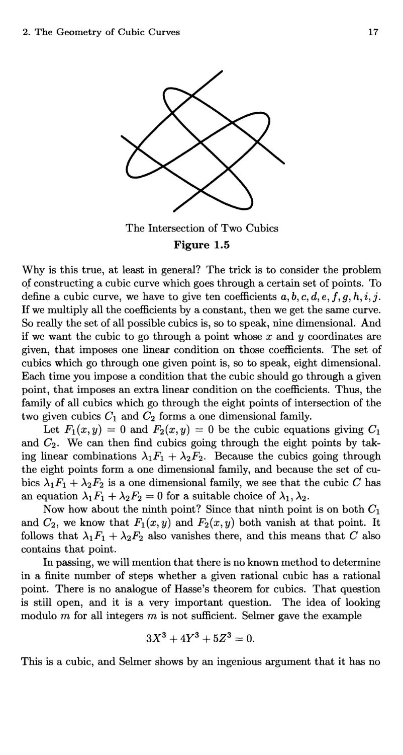
2. The Geometry of Cubic Curves 17
The Intersection of Two Cubics
Figure 1.5
Why is this true, at least in general? The trick is to consider the problem
of constructing a cubic curve which goes through a certain set of points. To
define a cubic curve, we have to give ten coefficients а, Ь, с, d, e,/, g, /i, i,j.
If we multiply all the coefficients by a constant, then we get the same curve.
So really the set of all possible cubics is, so to speak, nine dimensional. And
if we want the cubic to go through a point whose x and у coordinates are
given, that imposes one linear condition on those coefficients. The set of
cubics which go through one given point is, so to speak, eight dimensional.
Each time you impose a condition that the cubic should go through a given
point, that imposes an extra linear condition on the coefficients. Thus, the
family of all cubics which go through the eight points of intersection of the
two given cubics C\ and C2 forms a one dimensional family.
Let Fi(x,y) = 0 and F2(x,y) = 0 be the cubic equations giving C\
and C2. We can then find cubics going through the eight points by tak-
taking linear combinations AiFi + X2F2. Because the cubics going through
the eight points form a one dimensional family, and because the set of cu-
cubics Ai-Fi + X2F2 is a one dimensional family, we see that the cubic С has
an equation X\Fi -f X2F2 = 0 for a suitable choice of Ai, Л2.
Now how about the ninth point? Since that ninth point is on both C\
and C2, we know that F\{x,y) and Fi(x,y) both vanish at that point. It
follows that X\F\ + X2F2 also vanishes there, and this means that С also
contains that point.
In passing, we will mention that there is no known method to determine
in a finite number of steps whether a given rational cubic has a rational
point. There is no analogue of Hasse's theorem for cubics. That question
is still open, and it is a very important question. The idea of looking
modulo m for all integers m is not sufficient. Selmer gave the example
3X3 + AY3 + 5Z3 = 0.
This is a cubic, and Selmer shows by an ingenious argument that it has no
18 I. Geometry and Arithmetic
integer solutions other than @,0,0). However, one can check that for every
integer ra, the congruence
SX3 + 4У3 + 5Z3 = 0 (mod m)
has a solution in integers with no common factor. So for general cubics, the
existence of a solution modulo m for all m does not ensure that a rational
solution exists. We will leave this difficult problem aside, and assume that
we have a cubic which has a rational point O.
We want to reformulate Mordell's theorem in a way which has great
aesthetic and technical advantages. If we have any two rational points on
a rational cubic, say P and Q, then we can draw the line joining P to Q,
obtaining the third point which we denoted P * Q. This has the flavor
of many of the constructions you have studied in modern algebra. If we
consider the set of all rational points on the cubic, we can say that set has
a law of composition. Given any two points P, Q, we have defined a third
point P * Q. We might ask about the algebraic structure of this set and
this composition law; for example, is it a group? Unfortunately, it is not a
group; to start with, it is fairly clear that there is no identity element.
However, by playing around with it a bit, we can make it into a group
in such a way that the given rational point О becomes the zero element of
the group. We will denote the group law by + because it is going to be a
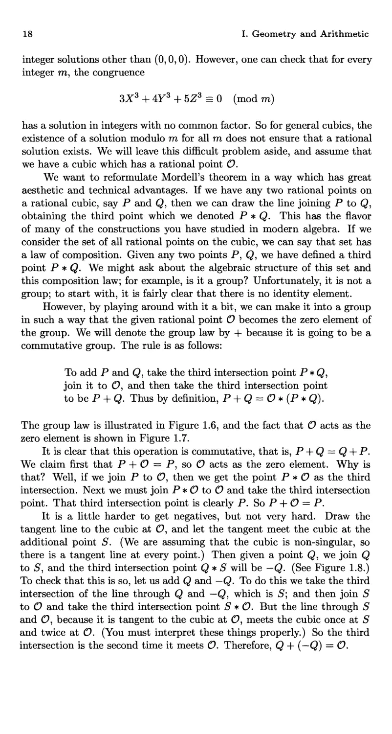
commutative group. The rule is as follows:
To add P and Q, take the third intersection point P*Q,
join it to O, and then take the third intersection point
to be P + Q. Thus by definition, P + Q = O*(P*Q).
The group law is illustrated in Figure 1.6, and the fact that О acts as the
zero element is shown in Figure 1.7.
It is clear that this operation is commutative, that is, P + Q — Q + P.
We claim first that P + О = P, so О acts as the zero element. Why is
that? Well, if we join P to 0, then we get the point P * О as the third
intersection. Next we must join P * О to О and take the third intersection
point. That third intersection point is clearly P. So P + О = P.
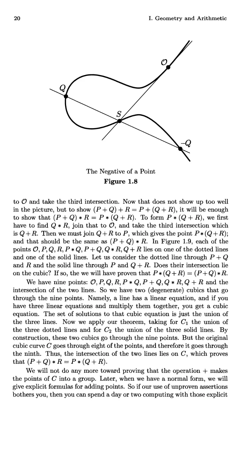
It is a little harder to get negatives, but not very hard. Draw the
tangent line to the cubic at 0, and let the tangent meet the cubic at the
additional point S. (We are assuming that the cubic is non-singular, so
there is a tangent line at every point.) Then given a point Q, we join Q
to 5, and the third intersection point Q * S will be — Q. (See Figure 1.8.)
To check that this is so, let us add Q and — Q. To do this we take the third
intersection of the line through Q and —Q, which is S; and then join S
to О and take the third intersection point S * O. But the line through S
and O, because it is tangent to the cubic at O, meets the cubic once at S
and twice at O. (You must interpret these things properly.) So the third
intersection is the second time it meets O. Therefore, Q -f (—Q) = O.
2. The Geometry of Cubic Curves
19
The Group Law on a Cubic
Figure 1.6
P+O =
Verifying О Is the Zero Element
Figure 1.7
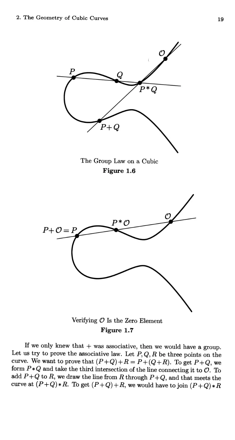
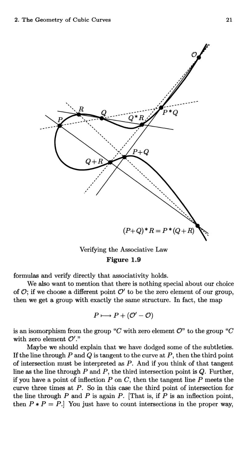
If we only knew that + was associative, then we would have a group.
Let us try to prove the associative law. Let P, Q, R be three points on the
curve. We want to prove that (P + Q)+R = P + (Q + R). To get P+Q, we
form P*Q and take the third intersection of the line connecting it to O. To
add P+Q to Д, we draw the line from R through P+Q, and that meets the
curve at (P + Q) * R- To get (P + Q)+ Д, we would have to join (P + Q) * R
20 I. Geometry and Arithmetic
The Negative of a Point
Figure 1.8
to О and take the third intersection. Now that does not show up too well
in the picture, but to show (P + Q) + R = P + (Q + R), it will be enough
to show that (P + Q) * R = P * (Q + R). To form P * (Q + R), we first
have to find Q * R, join that to 0, and take the third intersection which
is Q + R. Then we must join Q + R to P, which gives the point P* (Q + R);
and that should be the same as (P + Q) * R. In Figure 1.9, each of the
points O,P,Q,R,P*Q,P + Q,Q*R,Q + R lies on one of the dotted lines
and one of the solid lines. Let us consider the dotted line through P + Q
and R and the solid line through P and Q + R. Does their intersection lie
on the cubic? If so, the we will have proven that P*(Q + R) = (P + Q)*R.
We have nine points: O,P,Q,R,P * Q,P + Q,Q * R,Q + R and the
intersection of the two lines. So we have two (degenerate) cubics that go
through the nine points. Namely, a line has a linear equation, and if you
have three linear equations and multiply them together, you get a cubic
equation. The set of solutions to that cubic equation is just the union of
the three lines. Now we apply our theorem, taking for C\ the union of
the three dotted lines and for Ci the union of the three solid lines. By
construction, these two cubics go through the nine points. But the original
cubic curve С goes through eight of the points, and therefore it goes through
the ninth. Thus, the intersection of the two lines lies on C, which proves
that (P + Q)*R = P*(Q + R).
We will not do any more toward proving that the operation + makes
the points of С into a group. Later, when we have a normal form, we will
give explicit formulas for adding points. So if our use of unproyen assertions
bothers you, then you can spend a day or two computing with those explicit
2. The Geometry of Cubic Curves
21
Verifying the Associative Law
Figure 1.9
formulas and verify directly that associativity holds.
We also want to mention that there is nothing special about our choice
of O\ if we choose a different point O' to be the zero element of our group,
then we get a group with exactly the same structure. In fact, the map
is an isomorphism from the group UC with zero element 0" to the group UC
with zero element O1'."
Maybe we should explain that we have dodged some of the subtleties.
If the line through P and Q is tangent to the curve at P, then the third point
of intersection must be interpreted as P. And if you think of that tangent
line as the line through P and P, the third intersection point is Q. Further,
if you have a point of inflection P on C, then the tangent line P meets the
curve three times at P. So in this case the third point of intersection for
the line through P and P is again P. [That is, if P is an inflection point,
then P * P = P.] You just have to count intersections in the proper way,
22 I. Geometry and Arithmetic
and it is clear why if you think of the points varying a little bit. But to put
everything on solid ground is a big task. If you are going into this business,
it is important to start with better foundations and from a more general
point of view. Then all these questions would be taken care of.
How does this allow us to reformulate Mordell's theorem? Mordell's
theorem says that we can get all of the rational points by starting with
a finite set, drawing lines through those points to get new points, then
drawing lines through the new points to get more points, and so on. In
terms of the group law, this says that the group of rational points is finitely
generated. So we have the following statement of Mordell's theorem.
Mordell's Theorem. If a non-singular plane cubic
curve has a rational point, then the group of rational
points is finitely generated.
This version is obviously technically a much better form because we can
use a little elementary group theory, nothing very deep, but a convenient
device in the proof.
3. Weierstrass Normal Form
We are going to prove Mordell's theorem as Mordell did, using explicit for-
formulas for the addition law. To make these formulas as simple as possible,
it is important to know that any cubic with a rational point can be trans-
transformed into a certain special form called Weierstrass normal form. We will
not completely prove this, but we will give enough of an indication of the
proof so that anyone who is familiar with projective geometry can carry
out the details. (See Appendix A for an introduction to projective geom-
geometry.) Also, we will work out a specific example to illustrate the general
theory. After that, we will restrict attention to cubics which are given in
the Weierstrass form, which classically consists of equations that look like
y2 = 4ж3 - g2x - gs.
We will also use the slightly more general equation
y2 = xs + ax2 + bx + c,
and will call either of them Weierstrass form. What we need to show is that
any cubic is, as one says, birationally equivalent to a cubic of this type. We
will now explain what this means, assuming that the reader knows a (very)
little bit of projective geometry.
We start with a cubic curve, which we will think of as being in the
projective plane. The idea is to choose axes in the projective plane so that
the equation for the curve has a simple form. We assume we are given
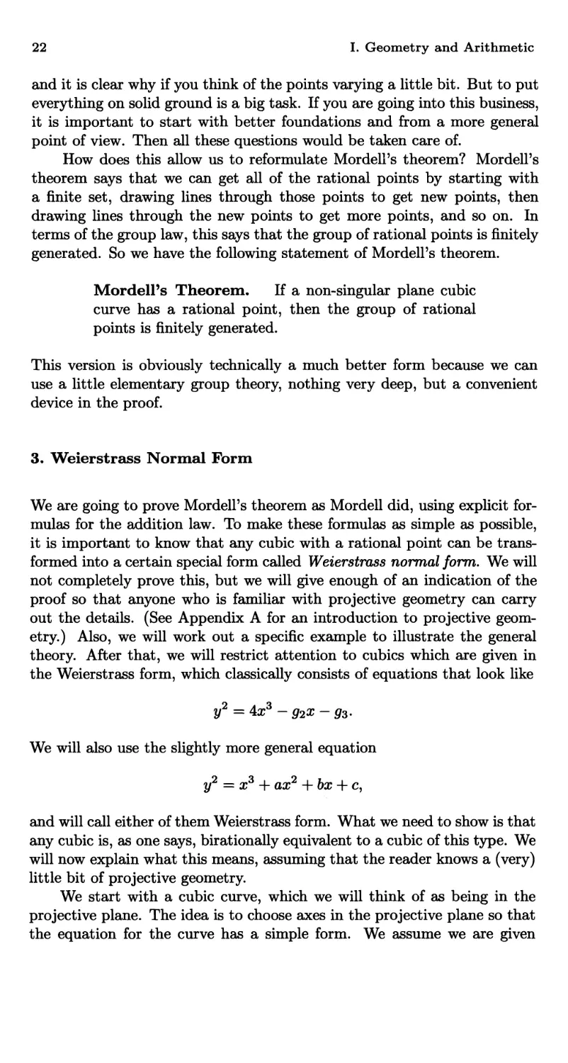
3. Weierstrass Normal Form 23
Choosing Axes to Put С into Weierstrass Form
Figure 1.10
a rational point О on C, so we begin by talcing Z = 0 to be the tangent
line to С at O. This tangent line intersects С at one other point, and
we take the X = 0 axis to be tangent to С at this new point. Finally, we
choose Y = 0 to be any line (other than Z = 0) which goes througn 0. (See
Figure 1.10. We are assuming that О is not a point of inflection; otherwise
we can take X = 0 to be any line not containing O.)
X Y
If we choose axes in this fashion and let x = ■—- and у = —, then
we get some linear conditions on the form the equation will take in these
coordinates. This is called a projective transformation. We will not work
out the algebra, but will just tell you that at the end the equation for С
takes the form
xy2 + (ax + b)y = ex2 + dx + e.
Next we multiply through by ж,
(xyJ + (ax + b)a;2/ = ex3 + dx2 + ex.
Now if we give a new name to жу, we will just call it у again, then we obtain
y2 + (ax + b)y = cubic in ж.
Replacing уЪуу— ^(аж + Ь), another linear transformation which amounts
to completing the square on the left-hand side of the equation, we obtain
y2 = cubic in x.
The cubic in x might not have leading coefficient 1, but we can adjust that
by replacing x and у by Xx and A2y, where A is the leading coefficient of
24 I. Geometry and Arithmetic
the cubic. So we do finally get an equation in Weierstrass form. And if
we want to get rid of the x2 term in the cubic, replace x by x — a for an
appropriate choice of a.
Tracing through all of the transformations from the original coordi-
coordinates to the new coordinates, we see that the transformation is not linear,
but it is rational. In other words, the new coordinates are given as ratios of
polynomials in the old coordinates. Hence, rational points on the original
curve correspond to rational points on the new curve.
An example should make all of this clear. Suppose we start with a
cubic of the form
u3 +v3 = a,
where a is a given rational number. The homogeneous form of this equation
is U^+V3 = aW3, so in the projective plane this curve contains the rational
point [1,-1,0]. Applying the above procedure (note that [1,-1,0] is an
inflection point) leads to new coordinates x and у which are given in terms
of и and v by the rational functions
12a u-v
x— and у = 36a .
U+V U+V
If you work everything out, you will see that x and у satisfy the Weierstrass
equation
2/2=s3-432a2.
Further, the process can be inverted, and one finds that и and v can be
expressed in terms of x and у by
36a + у , 36a - у
и = — and v = — .
6x 6x
Thus if we have a rational solution to u3+v3 = a, then we get rational x
and у which satisfy the equation y2 = xs — 432a2. And conversely, if we
have a rational solution of y2 = x3 — 432a2, then we get rational numbers
satisfying u3 + v3 = a. Of course, if и = —v, then the denominator in the
expression for x and у is zero; but there are only a finite number of such
exceptions, and they are easy to find. So the problem of finding rational
points on u3 + v3 = a is the same as the problem of finding rational points
on y2 = x3 — 432a2. And the general argument sketched above indicates
that the same is true for any cubic. Of course, the normal form has an
entirely different shape from the original equation. But there is a one-to-one
correspondence between the rational points on one curve and the rational
points on the other (up to a few easily catalogued exceptional points). So
the problem of rational points on general cubic curves having one rational
point is reduced to studying rational points on cubic curves in Weierstrass
normal form.
The transformations we used to put the curve in normalized form do
not map straight lines to straight lines. Since we defined the group law
3. Weierstrass Normal Form
25
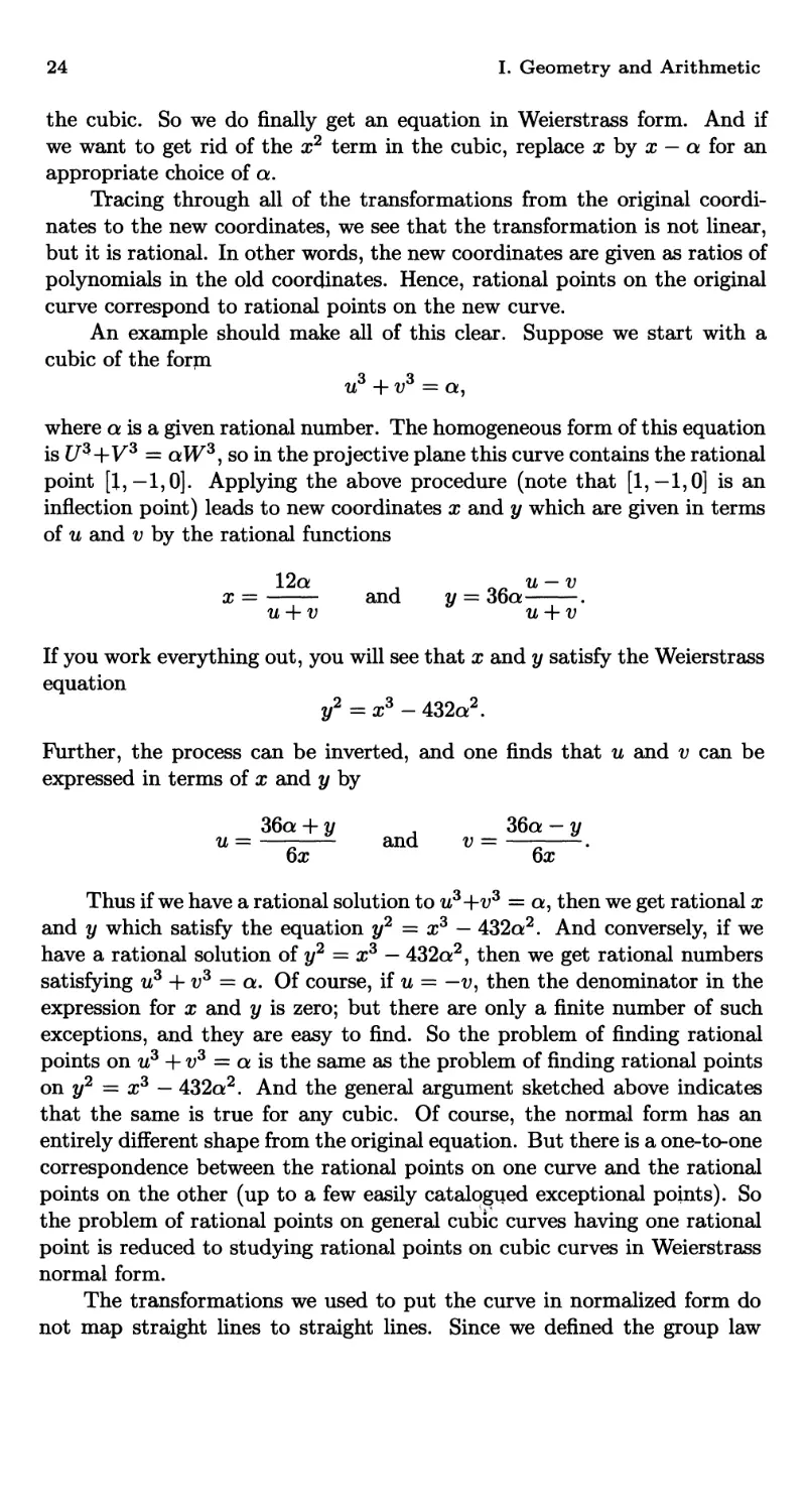
A Cubic Curve with One Real Component
Figure 1.11
on our curve using lines connecting points, it is not at all clear that our
transformation preserves the structure of the group. (That is, is our trans-
transformation a homomorphism?) It is, but that is not at all obvious. The
point is that our description of addition of points on the curve is not a
good one, because it seems to depend on the way the curve is embedded
in the plane. But in fact the addition law is an intrinsic operation which
can be described on the curve and is invariant under birational transfor-
transformation. This follows from basic facts about algebraic curves, but is not so
easy (virtually impossible?) to prove simply by manipulating the explicit
equations.
A cubic equation in normal form looks like
y2 = f(x) = xs + ax2 + bx + с
Assuming that the (complex) roots of f(x) are distinct, such a curve is
called an elliptic curve. (More generally, any curve birationally equivalent
to such a curve is called an elliptic curve.) Where does this name come
from, because these curves are certainly not ellipses? The answer is that
these curves arose in studying the problem of how to compute the arc length
of an ellipse. If one writes down the integral which gives the arc length of an
ellipse and makes an elementary substitution, the integrand will involve the
square root of a cubic or quartic polynomial. So to compute the arc-length
of an ellipse, one integrates a function involving у = y/f(x), and the answer
is given in terms of certain functions on the "elliptic" curve y2 = f(x).
Now we take the coefficients a, 6, с of f(x) to be rational, so in partic-
particular they are real; hence, the polynomial f(x) of degree 3 has at least one
real root. In real numbers we can factor it as
f(x) = (x - a)(x2 + /3x + 7) with a, /?,7 real.
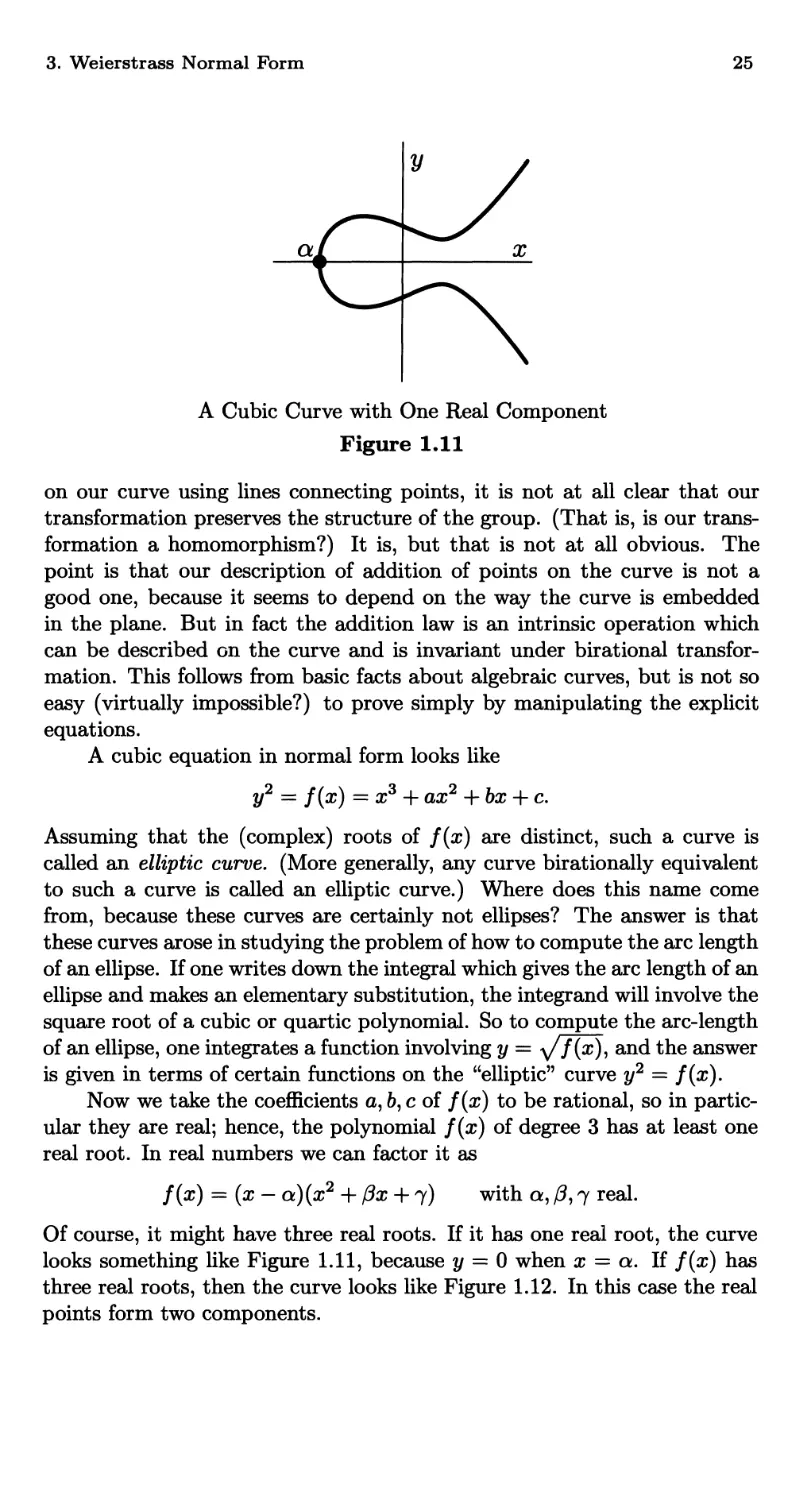
Of course, it might have three real roots. If it has one real root, the curve
looks something like Figure 1.11, because у = 0 when x = a. If f(x) has
three real roots, then the curve looks like Figure 1.12. In this case the real
points form two components.
26
I. Geometry and Arithmetic
A Cubic Curve with Two Real Components
Figure 1.12
All of this is valid, provided the roots of f(x) are distinct. What is
the significance of that condition? We have been assuming all along that
our cubic curve is non-singular. If we write the equation as F(x,y) =
y2 — f(x) = 0 and take partial derivatives,
OF
OF
then by definition the curve is non-singular, provided that there is no point
on the curve at which the partial derivatives vanish simultaneously. This
will mean that every point on the curve has a well-defined tangent line. Now
if these partial derivatives were to vanish simultaneously at a point (жо, 2/о)
on the curve, then yo — 0, and hence f(x0) = 0, and hence f(x) and f'(x)
have the common root xq. Thus x0 is a double root of /. Conversely, if /
has a double root жо, then (жо, 0) will be a singular point on the curve.
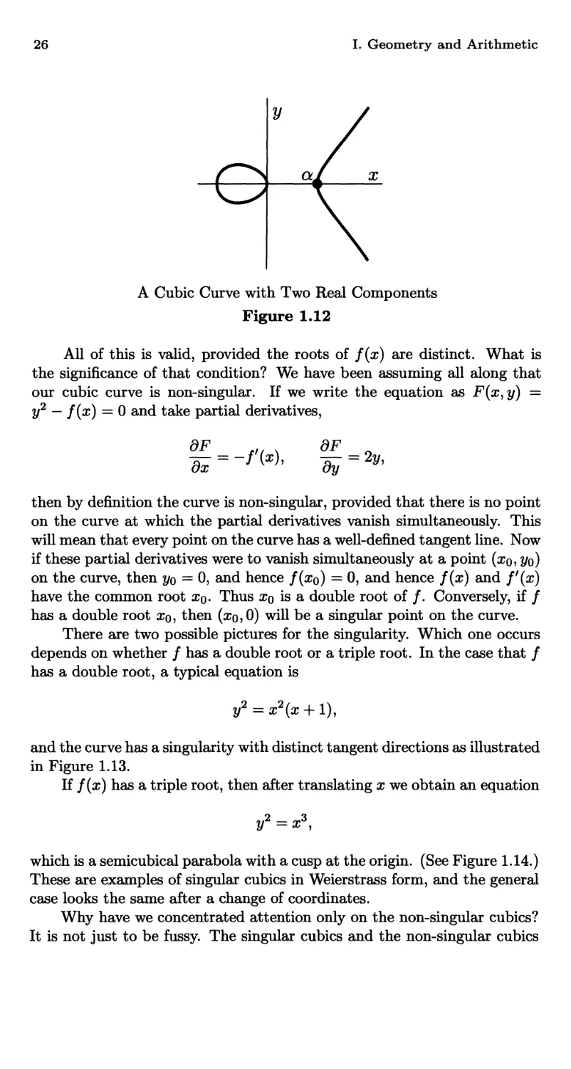
There are two possible pictures for the singularity. Which one occurs
depends on whether / has a double root or a triple root. In the case that /
has a double root, a typical equation is
and the curve has a singularity with distinct tangent directions as illustrated
in Figure 1.13.
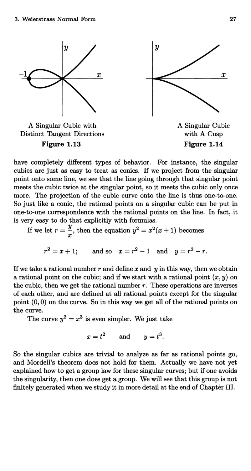
If f(x) has a triple root, then after translating x we obtain an equation
which is a semicubical parabola with a cusp at the origin. (See Figure 1.14.)
These are examples of singular cubics in Weierstrass form, and the general
case looks the same after a change of coordinates.
Why have we concentrated attention only on the non-singular cubics?
It is not just to be fussy. The singular cubics and the non-singular cubics
3. Weierstrass Normal Form
27
-1
A Singular Cubic with
Distinct Tangent Directions
Figure 1.13
A Singular Cubic
with A Cusp
Figure 1.14
have completely different types of behavior. For instance, the singular
cubics are just as easy to treat as conies. If we project from the singular
point onto some line, we see that the line going through that singular point
meets the cubic twice at the singular point, so it meets the cubic only once
more. The projection of the cubic curve onto the line is thus one-to-one.
So just like a conic, the rational points on a singular cubic can be put in
one-to-one correspondence with the rational points on the line. In fact, it
is very easy to do that explicitly with formulas.
ii
If we let r = -, then the equation y2 = x2(x + 1) becomes
x
r2 = x + 1; and so x = r2 — 1 and у = r3 —
r.
If we take a rational number r and define x and у in this way, then we obtain
a rational point on the cubic; and if we start with a rational point (ж, у) on
the cubic, then we get the rational number r. These operations are inverses
of each other, and are defined at all rational points except for the singular
point @,0) on the curve. So in this way we get all of the rational points on
the curve.
The curve y2 = xs is even simpler. We just take
= t2
and
= t3.
So the singular cubics are trivial to analyze as far as rational points go,
and Mordell's theorem does not hold for them. Actually we have not yet
explained how to get a group law for these singular curves; but if one avoids
the singularity, then one does get a group. We will see that this group is not
finitely generated when we study it in more detail at the end of Chapter III.
28 I. Geometry and Arithmetic
4. Explicit Formulas for the Group Law
We are going to look at the group of points on a non-singular cubic a little
more closely. If you are familiar with projective geometry, then you will
not have any trouble; and if not, then you will have to accept a point at
infinity, but only one. (If you have never studied any projective geometry,
you might also want to look at the first two sections of Appendix A.)
We start with the equation
y2 = xs + ax2 + bx + с
X Y
and make it homogeneous by setting x = — and у — —, yielding
Zi Zi
Y2Z = Xs + aX2Z + bXZ2 + cZs.
What is the intersection of this cubic with the line at infinity Z = 0?
Substituting Z = 0 into the equation gives X3 = 0, which has the triple
root X = 0. This means that the cubic meets the line at infinity in three
points, but the three points are all the same! So the cubic has exactly
one point at infinity, namely, the point at infinity where vertical lines (x =
constant) meet. The point at infinity is an inflection point of the cubic, and
the tangent line at that point is the line at infinity, which meets it there
with multiplicity three. And one easily checks that the point at infinity is
a non-singular point by looking at the partial derivatives there. So for a
cubic in Weierstrass form there is one point at infinity; we will call that
point O.
The point О is counted as a rational point, and we take it as the zero
element when we make the set of points into a group. So to make the game
work, we have to make the convention that the points on our cubic consist
of the ordinary points in the ordinary affine xy plane together with one
other point О that you cannot see. And now we find it is really true that
every line meets the cubic in three points; namely, the line at infinity meets
the cubic at the point О three times. A vertical line meets the cubic at
two points in the xy plane and also at the point O. And a non-vertical line
meets the cubic in three points in the xy plane. Of course, we may have to
allow x and у to be complex numbers.
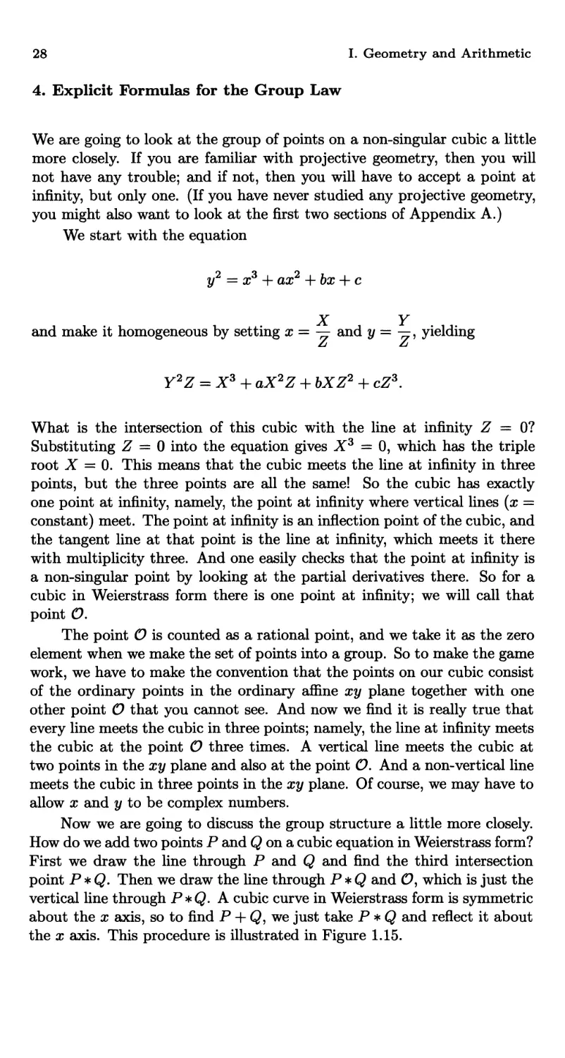
Now we are going to discuss the group structure a little more closely.
How do we add two points P and Q on a cubic equation in Weierstrass form?
First we draw the line through P and Q and find the third intersection
point P * Q. Then we draw the line through P * Q and 0, which is just the
vertical line through P*Q. A cubic curve in Weierstrass form is symmetric
about the x axis, so to find P + Q, we just take P * Q and reflect it about
the x axis. This procedure is illustrated in Figure 1.15.
4. Explicit Formulas for the Group Law
29
У
Adding Points on a Weierstrass Cubic
Figure 1.15
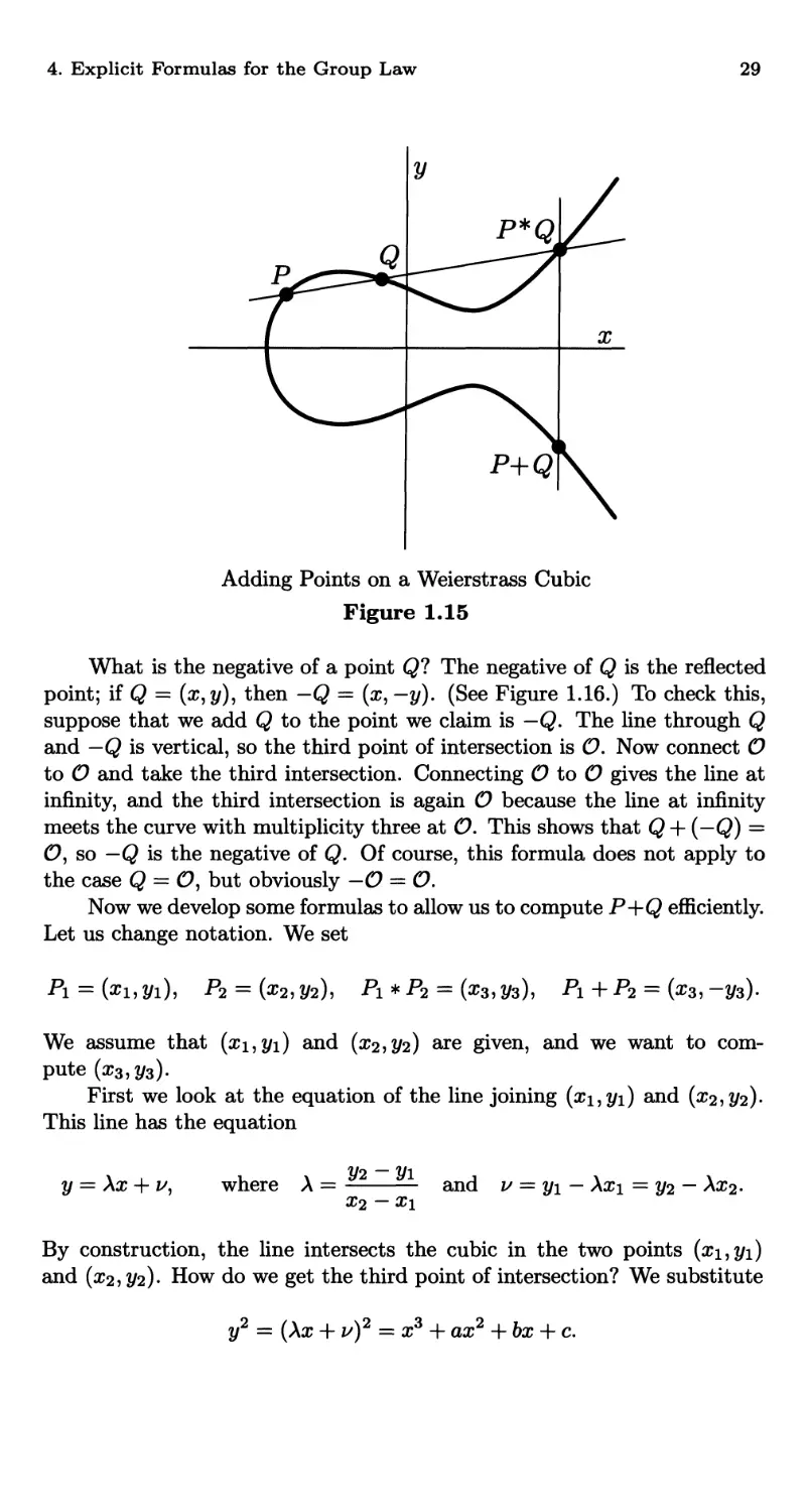
What is the negative of a point Q? The negative of Q is the reflected
point; if Q = (ж, 2/), then — Q = (ж, —у). (See Figure 1.16.) To check this,
suppose that we add Q to the point we claim is — Q. The line through Q
and — Q is vertical, so the third point of intersection is O. Now connect О
to О and take the third intersection. Connecting О to О gives the line at
infinity, and the third intersection is again О because the line at infinity
meets the curve with multiplicity three at O. This shows that Q + (—Q) =
0, so — Q is the negative of Q. Of course, this formula does not apply to
the case Q = 0, but obviously -O = O.
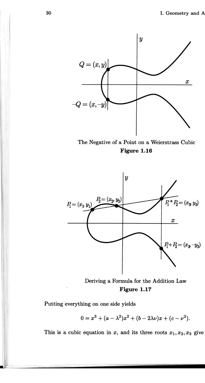
Now we develop some formulas to allow us to compute P+Q efficiently.
Let us change notation. We set
Pi =
Pi = (x2,2/2), Pi * Рч = (ж3, уз),
= (я?3, -2/з).
We assume that (ж 1,2/1) and (^2,2/2) are given, and we want to com-
compute (ж3,2/з).
First we look at the equation of the line joining (#1,2/1) and (#2,2/2)-
This line has the equation
2/ = Xx + 1/, where A =
and v = 2/1 — A#i = 2/2 —
By construction, the line intersects the cubic in the two points (#1,2/1)
and (#2,2/2)- How do we get the third point of intersection? We substitute
у2 = (Ах + vf = х3
с.
30
I. Geometry and A
У
The Negative of a Point on a Weierstrass Cubic
Figure 1.16
Deriving a Formula for the Addition Law
Figure 1.17
Putting everything on one side yields
0 = x3 + (a - \2)x2 + (b - 2Xu)x + (c - i/2).
This is a cubic equation in x, and its three roots
4. Explicit Formulas for the Group Law 31
coordinates of the three intersections. Thus,
x3 + (a - X2)x2 + (b - 2\v)x + (c - v2) = (x - хг)(х - x2)(x - x3).
Equating the coefficients of the x2 term on either side, we find that A2 — a —
#1 +#2 + #3> and so
xs = A2 - a - xi - x2, уз = Аж3 + v.
These formulas are the most efficient way to compute the sum of two points.
Let us do an example. We look at the cubic curve
y2 = xs + 17
which has the two points Pi = (—1,4) and P2 = B,5). To compute Pi +P2
we first find the line through the two points, у = ^x + ^, so A = |
and v = Щ. Next ж3 = A2 - x2 - xi = -§ and y3 = Аж3 + v = Щ. Finally
we find that Pi + P2 = (ж3, —y3) = (—|, —Щ-\ So computations really
are not that bad.
The formulas we gave earlier involve the slope A of the line connecting
the two points. What if the two points are the same? So suppose that we
have Po = (#o,2/o) and we want to find Po + Po = 2P0. We need to find
the line joining Po to Po. Because x\ = x2 and y\ = y2, we cannot use our
formula for A. But the recipe we described for adding a point to itself says
that the line joining Po to Po is the tangent line to the cubic at Po. From
the relation y2 = f(x) we find by implicit differentiation that
dy _ f'(x)
dx~ 2y '
so that is what we use when we want to double a point.
Continuing with our example curve у2 = ж3 + 17 and point Pi =
(-1,4), we compute 2Pi as follows. First, A = /'0&i)/2yi = /;(-l)/8 = §.
Then, once we have a value for A, we just substitute into the formulas as
above, eventually finding that 2Pi = (Щ, -Щ-).
Sometimes it is convenient to have an explicit expression for 2P in
terms of the coordinates for P. If we substitute A = f'(x)/2y into the
formulas given earlier, put everything over a common denominator, and
replace y2 by /(ж), then we find that
-ft/ ч x4 - 2bx2 - 8cx + b2 - 4ac
x coordinate of 2(ж, у) = » —2———— .
Ax6 + Aax2 + 4bx + Ac
This formula for xBP) is often called the duplication formula. It will come
in very handy later for both theoretical and computational purposes. We
will leave it to you verify this formula, as well as to derive a companion
formula for the у coordinate of 2P.
32 I. Geometry and Arithmetic
These are the basic formulas for the addition of points on a cubic when
the cubic is in Weierstrass form. We will use the formulas extensively to
prove many facts about rational points on cubic curves, including Mordell's
theorem. Further, if you were not satisfied with our incomplete proof that
the addition law is associative, you can just take three points at random
and compute. Of course, there are an awful lot of special cases to consider,
such as when one of the points is the negative of the other or two of the
points coincide. But in a few days you will be able to check associativity
using these formulas. So we need say nothing more about the proof of the
associative law!
Exercises
1.1. (a) If P and Q are distinct rational points in the (x,y) plane, prove
that the line connecting them is a rational line.
(b) If L\ and L2 are distinct rational lines in the (#, у) plane, prove
that their intersection is a rational point (or empty).
1.2. Let С be the conic given by the equation
F(x, y) = ax2 + bxy + cy2 + dx + ey + / = 0,
and let 6 be the determinant
Ba b d
b 2c e
d e 2/,
(a) Show that if 6 Ф 0, then С has no singular points. That is, show
that there are no points (#, y) where
ч dF, ч dF,
^'^ = ~дх^Х'У' = ~ду^Х^ =
(b) Conversely, show that if 8 = 0 and b2 — Aac ф 0, then there is a
unique singular point on C.
(c) Let L be the line у = ax + /3 with а ф 0. Show that the intersec-
intersection of L and С consists of either zero, one, or two points.
(d) Determine the conditions on the coefficients which ensure that the
intersection LnC consists of exactly one point. What is the geometric
significance of these conditions? (Note. There will be more than one
case.)
1.3. Let С be the conic given by the equation
x2 - Sxy + 2y2 - x + 1 = 0.
(a) Check that С is non-singular (cf. the previous exercise).
(b) Let L be the line у = ax + /3. Suppose that the intersection LnC
contains the point P$ = (xo, yo). Assuming that LnC consists of two
distinct points, find the second point of LnC in terms of a, /3, xo, 3/0-
(c) If L is a rational line and Pq is a rational point (i.e., a, /3, xo, 2/0 €
Q), prove that the second point of L П С is also a rational point.
Exercises 33
1.4. Find all primitive integral right triangles whose hypotenuse has length
less than 30.
1.5. Find all of the rational points on the circle
by projecting from the point A,1) onto an appropriate rational line.
(Your formulas will be simpler if you are clever in your choice of the
line.)
1.6. (a) Let a, b, c, d, e, / be non-zero real numbers. Use the substitu-
substitution t = tan@/2) to transform the integral
a + b cos 0 + с sin 0
du
into the integral of a rational function of t.
(b) Evaluate the integral
a + bcos0 + csin0
1 + cos 0 + sin 0
1.7. For each of the following conies, either find a rational point or prove
that there are no rational points.
(a) x2 + y2 = 6
(b) 3x2 + by2 = 4
(c) Sx2 + 6</2 = 4
1.8. Prove that for every exponent e > 1, the congruence
z2 + l = 0(mod5e)
has a solution xe G Z/5eZ. Prove further that these solutions can be
chosen to satisfy
x\ = 2 (mod 5), and #e+i = xe (mod 5e) for all e > 1.
(This is equivalent to showing that the equation x2 + 1 = 0 has a
solution in the 5-adic numbers. It is a special case of Hensel's lemma.
Hint Use induction on e.)
1.9. Let C\ and С% be the cubics given by the following equations:
d : x3 + 2y3 - x - 2y = 0, C2 : 2x3 - y3 - 2x + у = 0.
(a) Find the nine points of intersection of C\ and C^.
(b) Let {@,0), Pi,..., Ps} be the nine points from part (a). Prove
that if a cubic curve goes through Pi,... ,P8, then it must also go
through the ninth point @,0).
34 I. Geometry and Arithmetic
1.10. Define a composition law on the points of a cubic С by the following
rule as described in the text: Given P,Q e C, then P*Q is the point
on С so that P, Q, and P * Q are colinear.
(a) Explain why this law is commutative, P *Q = Q * P.
(b) Prove that there is no identity element for this composition law;
that is, there is no element Po £ С such that P0*P = P for all P eC.
(c) Prove that this composition law is not associative; that is, in
general, P * (Q * R) ^ (P * Q) * R.
(d) Explain why P*(P*Q) = Q.
(e) Suppose that the line through О and 5 is tangent to С at O.
Explain why
O*(Q*(Q*S))= O.
(This is an algebraic verification that the point we called — Q is the
additive inverse of Q.)
1.11. Let 5 be a set with a composition law * satisfying the following two
properties:
(i) P*Q = Q*P forallP,QeS.
(ii) P*(P*Q) = Q forallP,QeS.
Fix an element О G 5, and define a new composition law + by the
rule
= O*(P*Q).
(a) Prove that + is commutative and has О as identity element
(i.e., prove that P + Q = Q + P and P + О = P).
(b) Prove that for any given P,Q e S, the equation X + P = Q
has the unique solution X = P * (Q * O) in 5. In particular, if we
define —P to be P * (O * 0), then —P is the unique solution in 5 of
the equation X + P = O.
(c) Prove that + is associative (and so E, +) is a group) if and only
if
(iii) R * (O * (P * Q)) = P * (O * (Q * R)) for all P,Q,Re S.
(d) Let O' G S be another point, and define a composition law +'
by P+; Q = O' * (P* Q). Suppose that both + and +' are associative,
so we obtain two group structures E, +) and E, +') on 5. Prove that
the map
Pi > О * {О1 * P)
is a (group) isomorphism from E,+) to E, +').
(e) * Find a set 5 with a composition law * satisfying (i) and (ii)
such that E, +) is not a group.
Exercises 35
1.12. The cubic curve u3+v3 = a (with а ф 0) has a rational point [1, —1,0]
at infinity. (That is, this is a point on the homogenized equation U3 +
V3 = aW3.) Taking this rational point to be 0, we can make the
points on the curve into a group.
(a) Derive a formula for the sum Pi + P2 of two points Pi = (ui, v\)
and P2 = (^25^2)-
(b) Derive a duplication formula for 2P in terms of P = (u, v).
1.13. (a) Verify that if и and v satisfy the relation u3 + v3 = a, then the
quantities
12a , пл и — v
x = and у = 36а
u+v u + v
satisfy the relation y2 = x3 — 432a2.
(b) Part (a) gives a birational transformation from the curve u3+v3 =
a to the curve у2 = ж3—432a2. Each of these cubic curves has a group
law defined on it. Prove that the birational transformation described
in (a) is an isomorphism of groups.
1.14. Let С be the cubic curve u3 + v3 = и + v +1. In the projective plane,
this curve has a point [1, —1,0] at infinity. Find rational functions x =
х(щу) and у = y(u,v) so that x and у satisfy a cubic equation in
Weierstrass normal form with the given point still at infinity.
1.15. Let g(t) be a quartic polynomial with distinct (complex) roots, and
let a be a root of g(t). Let /3 Ф 0 be any number.
(a) Prove that the equations
13 2 02u
t — a' (t — aJ
give a birational transformation between the curve u2 = g(t) and the
curve y2 = /(#), where f(x) is the cubic polynomial
j(x) = g [a)px + 2# \а)Р x + q9 («)P ^ + 24^ \&)р .
(b) Prove that if g has distinct (complex) roots, then / also has
distinct roots, and so u2 = g(t) is an elliptic curve.
1.16. Let 0 < {3 < a, and let E be the ellipse
a2 + /32
(a) Prove that the arc length of E is given by the integral
pn/2
2
4a
/
Jo
36 I. Geometry and Arithmetic
for an appropriate choice of the constant к depending on a and /3.
(b) Check your value for к in (a) by verifying that when a = /3, the
integral yields the correct value for the arc length of a circle.
(c) Prove that the integral in (a) is also equal to
. f1 /1 - кЧ* M f1
4a / \ 7r-dt = 4;a /
io V 1-t2 Jo
1 - k2t2
(d) Prove that if the ellipse E is not a circle, then the equation
u2 = (l-t2)(l-k2t2)
defines an elliptic curve (cf. the previous exercise). Hence the problem
of determining the arc length of an ellipse comes down to evaluating
the integral
I
1 1 _
dt on the "elliptic" curve u2 = A - *2)A - k2t2).
1.17. Let С be a cubic curve in the projective plane given by the homoge-
homogeneous equation
Y2Z = X3 + aX2Z + bXZ2 + cZ3.
Verify that the point [0,1,0] at infinity is a non-singular point of С
1.18. The cubic curve
y2=x3 + 17
has the following five rational points:
P1 = (-2,3), P2 = (-1,4), P3 = B,5), P4 = D,9), P5 = (8,23).
(a) Show that P2, P4, and P5 can each be expressed as mP\ + nPs
for an appropriate choice of integers m and n.
(b) Compute the points
P6 = -Рг + 2P3 and P7 = 3Pi - P3.
(c) Notice that the points Р1,Р2,Рз,Р4,Р5,Рб,Рг all have integer
coordinates. There is exactly one more rational point on this curve
which has integer coordinates and у > 0. Find that point. (You
will probably need at least a programmable calculator or else a lot
of patience.)
(d) ** Prove the assertion in (c) that there are exactly eight rational
points (ж, у) on this curve with у > 0 and ж, у both integers. (This
is an extremely difficult problem, and you will almost certainly not
be able to do it with the tools we have developed. But it is also an
extremely interesting problem which is well worth thinking about.)
Exercises 37
1.19. Suppose that P = (#, у) is a point on the cubic curve
y2 = x3 + ax2 + Ъх + с.
(a) Verify that the x coordinate of the point 2P is given by the
duplication formula
x4 - 2bx2 -Sex- lac + b2
(b) Derive a similar formula for the у coordinate of 2P in terms of x
and y.
(c) Find a polynomial in x whose roots are the x coordinates of the
points P = (x, y) satisfying 3P = O. (Hint The relation 3P = О can
also be written IP = -P.)
(d) For the particular curve y2 = x3 + 1, solve the equation in (c) to
find all of the points satisfying 3P = O. Note you will have to use
complex numbers.
1.20. Consider the point P = C,8) on the cubic curve y2 = x3 - 43z +166.
Compute P, 2P, 3P, 4P, and 8P. Comparing 8P with P, what can
you conclude?
X HiJX 11
Points of Finite Order
1. Points of Order Two and Three
An element P of any group is said to have order m if
mP = P + P 4■ • • • + P = 0,
m summands
but m'P ф 0 for all integers 1 < m' < m. If such an m exists, then P has
finite order; otherwise it has infinite order. We begin our study of points
of finite order on cubic curves by looking at points of order two and order
three. As usual, we will assume that our non-singular cubic curve is given
by a Weierstrass equation
y2 = f(x) = x3 4- ax2 4- bx 4- c,
and that the point at infinity 0 is taken to be the zero element for the
group law.
Which points in our group satisfy 2P = 0, but P ^ O? Instead
of 2P = 0, it is easier to look at the equivalent condition P = —P.
Since —(ж, у) is just (x, — y), these are the points with у = 0:
Pi = (ab0), P2 = (a2,0), P3 = (a3,0),
where ai, a2, a3 are the roots of the cubic polynomial f{x). So if we allow
complex coordinates, there are exactly three points of order two, because
the non-singularity of the curve ensures that f(x) has distinct roots. If all
three roots of f(x) are real, then the picture looks like Figure 2.1.
1. Points of Order Two and Three
39
У
p p
Points of Order Two
Figure 2.1
If we take all of the points satisfying 2P = 0, including P = 0, then we
get the set {0, Pi, Рг, Р3}. It is easily seen that in any abelian group, the set
of solutions to the equation 2P = 0 forms a subgroup. So we have a group
of order four; and since every element has order one or two, it is obvious that
this group is the Four Group, a direct product of two groups of order two.
This means that the sum of any two of the points Pi, P2, P3 should equal
the third, which is obvious from the fact that the three points are collinear.
So now we know exactly what the group of points P such that 2P = 0 looks
like. If we allow complex coordinates, it is the Four Group; if we allow only
real coordinates, it is either the Four Group or cyclic of order two, depend-
depending on whether f(x) has three or one real root; and if we restrict our atten-
attention to rational coordinates, it is either the Four Group, cyclic of order two,
or trivial, depending on whether f(x) has three, one, or zero rational roots.
Next we look at the points of order three. Instead of 3P = 0, we
write 2P = -P, so a point of order 3 will satisfy xBP) = x(-P) = x(P).
Conversely, if P Ф 0 satisfies xBP) = x(P), then 2P = ±P, so either P =
0 (excluded by assumption) or 3P = 0. In other words, the points of order
three are exactly the points satisfying xBP) = x(P).
To find the points satisfying this condition, we use the duplication
formula and set the x coordinate of 2P equal to the x coordinate of P. If
we write P = (x, 2/), then we have shown in Chapter I that the x coordinate
of 2P equals
x4 - 2bx2 - Sex + b2 - 4ac
Ax3 + 4a#2 + 4foc + 4c
Setting this expression equal to #, cross-multiplying, and doing a little
algebra, we have completed the proof of part (c) of the following proposition.
40 II. Points of Finite Order
Points of Order Two and Three. Let С be the non-singular cubic
curve
С :y2 = f(x) = x3 + ах2 + Ъх + с.
[Recall that С is non-singular provided f(x) and f'(x) have no common
complex roots.]
(a) A point P = (x,y) 7^ О on С has order two if and only if у = 0.
(b) С has exactly four points of order dividing 2. These four points form
a group which is a product of two cyclic groups of order two.
(c) A point P = (x,y) ф О on С has order three if and only ifx is a root
of the polynomial
ip3(x) = Sx4 + 4az3 + 6bx2 + I2cx + Dac - b2).
(d) С has exactly nine points of order dividing 3. These nine points form
a group which is a product of two cyclic groups of order three.
Proof. (a,b) We proved these above.
(c) We proved (c) above except for a little bit of algebra, which we will
leave to you.
f'(xJ
(d) Because the x coordinate of 2P equals ;, \ — а — 2x, we see that an
alternative expression for фз(х) is
We claim that ^з(^) has four distinct (complex) roots. To verify this, we
need to check that фз(х) and ф'3(х) have no common roots. But
so a common root of ^з(#) and ^з(^) would be a common root of
2f(x)f"(x) - f{xf and 12/(x),
and so would be a common root of f(x) and f'(x). This is contrary to our
assumption that С is non-singular, so we conclude that ^з(^) indeed has
four distinct complex roots.
Let /?i, /?2, /?з, /?4 be the four complex roots of фз(х); and for each $,
let Si be one of the square roots 6i = у/ТЩ). Then from (c), the set
is the complete set of points of order three on C. Further, we observe that
no Si can equal zero, because otherwise the point (/3»,5») = (/?»,0) would
have order two, contradicting the fact that it has order three. Therefore,
this set contains exactly eight distinct points, so С contains eight points of
2. Real and Complex Points on Cubic Curves
41
A Cubic Curve with One Real Component
Figure 2.2
order three. The only other point on С with order dividing 3 is the point
of order one, namely 0, which completes the proof that С has exactly nine
points of order dividing 3.
Finally, we note that there is only one (abelian) group with nine ele-
elements such that every element has order dividing 3, namely, the product
of two cyclic groups of order three. □
So we now know that if we allow complex numbers, then the points of
order dividing three form a group of order nine which is the direct product
of two cyclic groups of order three. It turns out that the real points of order
three always form a cyclic group of order three, whereas the rational points
of order three form either a cyclic group of order three or the trivial group.
We will discuss this further in the next section.
There is also a geometric way to describe the points of order three; they
are inflection points, the points where the tangent line to the cubic has a
triple order contact. We can see that geometrically. To say that 2P = —P
means that when we draw the tangent at the point P, then take the third
intersection and connect it with 0, we get —P. Now that is the case only
if the third point of intersection of the tangent at P is the same point P.
So 2P = — P if and only if P is a point of inflection. Of course, this can
also be shown analytically; we will leave the analytic proof as an exercise.
2. Real and Complex Points on Cubic Curves
The real points on our cubic curve
y2 = f{x) = x3 + ax2 + Ъх + с
form either one or two components, depending on whether f(x) has one or
three real roots. We illustrated the case of three real roots in Figure 2.1,
and, of course, the case of one real root looks like Figure 2.2.
42 II. Points of Finite Order
This picture shows the real points, the points with real coordinates. Ac-
Actually, the equation for our cubic curve defines several sets of points. We
could write C(Q) for the set of points on the curve whose coordinates hap-
happen to be rational, C(R) for the points pictured above which have arbitrary
real coordinates, and C(C) for the set of pairs of complex numbers (x, y)
which satisfy the equation. And there is the point О at infinity, which we
take to be in all of these sets. We have made the points of the curve into a
group. This construction is purely algebraic, so it will work in any of these
three cases.
The points on the curve with complex coordinates form a group. The
points with real coordinates form a subgroup because if two points have
real coordinates, then so do their sum and difference. And since we are
assuming the coefficients a,b,c are rational numbers, it is even true that
the rational points form a subgroup of the group of real points.
So we have a big group and some subgroups:
{0} с C(Q) с C(R) с C(C).
To study the group of real points or complex points, one can use the meth-
methods of analysis.
It is obvious that the addition of real points on the curve is continuous.
So the group of real points is a one-dimensional Lie group; and this set is
in fact compact, although it does not look it because it has the point at
infinity. There is only one such connected group. Any one dimensional
compact connected Lie group is isomorphic to the group of rotations of
the circle; that is, the multiplicative group of complex numbers of absolute
value one. So if the group of real points on the curve is connected, then
it is isomorphic to the circle group; and in any case, the component of the
curve which contains the zero point is isomorphic to the circle group. And
from this description we can see immediately what the real points of finite
order look like.
If we think of the circle group as the multiplicative group of complex
numbers of absolute value one, then the points of finite order in that group
are the roots of unity. And for each integer m, the points of order dividing m
form a cyclic group of order m. Explicitly, this set of complex numbers is
е2(ш-1)тгг/т1
So the points of order dividing m in C(R) form a cyclic group of order m,
at least in the case that the group is connected.
If there are two connected components, then the group C(R) is the
direct product of the circle group with a group of order two. In this case,
there are two possibilities for the points of order dividing m. If m is odd,
we again get a cyclic group of order m; whereas if m is even, then we find
the direct product of a cyclic group of order two and a cyclic group of
order m.
2. Real and Complex Points on Cubic Curves 43
In particular, we see that the real points of order dividing 3 always
form a cyclic group of order three. Since we have seen that there are eight
points of order three, it is never possible for all of the complex points of
order three to be real, and certainly they cannot all be rational. Notice that
the x coordinates of the points of order three are the roots of the quartic
polynomial фъ (х) described in Section 1. This quartic has real coefficients,
so it has either zero, two, or four real roots. Because each value for x
gives two possible values for y, this shows that the curve has either zero,
four, or eight points of order three with real x coordinate. However, our
discussion shows that there must be exactly one real value of x for which
the two corresponding 2/'s are real. This can also be proven directly from
the equations, a task which we leave for the exercises.
Before continuing with our discussion of rational points, we briefly
digress to describe the structure of C(C). Substituting x — ^a for x, we can
eliminate the ax2 term; and then replacing x and у by 4x and %, we end
up with the classical form of Weierstrass equation:
у2 = 4х3 -д2Х~9з-
As always, the cubic polynomial on the right is assumed to have distinct
roots.
In the Weierstrass theory of elliptic functions, it is shown that whenever
you have two complex numbers #2> <7з so that the polynomial 4x3 — #2# — <7з
has distinct roots (i.e., such that g% —11 g\ ф 0), then you can find complex
numbers uj\, U2 (called periods) in the complex и plane by evaluating certain
definite integrals. These periods are R-linearly independent, and one looks
at the group formed by taking all of their Z-linear combinations:
L = Zcl?i + Zcl>2 = {^i^i + 712UJ2 : ni, П2 £ Z}.
(Such a subgroup of the complex plane is called a lattice.) Although there
are many choices for the generators ш^шъ of L, it turns out that the co-
coefficients <72 and #3 uniquely determine the group L itself. Conversely, the
group L uniquely determines #2 and #3 via the formulas
One uses the periods to define a function p(u) by the series
This meromorphic function is called the Weierstrass p function. It visibly
has poles at the points of L, and no other poles in the complex и plane.
Less obvious is the fact that p is doubly periodic; that is,
p(u + ui) = p(u) and p(u + U2) = p(u) for all complex numbers u.
44
II. Points of Finite Order
The Period Parallelogram
Figure 2.3
From this it follows that p(u + w) = p{u) for all и G С and all w G L.
Notice the similarity with trigonometric and exponential functions, which
have single periods: f(u) = sin(u) has the period 2тг, and f(u) = eu has
the period 2m.
This doubly periodic function p{u) satisfies the differential equation
/ /\2 л 3 i f dp
(p) =4p -д2р-дз, where p =-2-.
du
Thus for every complex number и we get a point
on the given curve, in general a point with complex coordinates. So we
obtain a map from the complex и plane to C(C). (Of course, we send the
points in L, which are the poles of p, to O.)
The facts about this map are as follows. The map is onto the curve;
every pair (x, y) of complex numbers satisfying y2 = 4x3 — g2x — g% comes
from some u. Because p is doubly periodic, the map cannot be one-to-one.
If и and v have the property that their difference u — v equals m\uji + ГП2Ш2
for some integers mi,m2 (i.e., if и - v G L), then P(u) = P(v). So instead
we just look at values of и which lie in the period parallelogram, which is
the parallelogram whose sides are the periods ш\ and UJ2- (See Figure 2.3.)
Then it is true that to a given point (ж, у) on the curve there is exactly
one и in the period parallelogram which is mapped to (x, y). (One must
make suitable conventions about the boundary of the parallelogram.)
Thus, the period parallelogram is mapped one-to-one onto the complex
points of the curve. The mapping и \—> P(u) has the property
Note that the sum щ + и^ is just the ordinary addition of complex num-
numbers, whereas P{u\) + P(u2) is the addition law on the cubic curve. This
2. Real and Complex Points on Cubic Curves
45
Points of Order Two on a Complex Torus
Figure 2.4
equation amounts to the famous addition formula for p(u). It says that
the functions p and p', evaluated at u\ + ^2, can be expressed rationally
in terms of their values at u\ and щ. The formulas are the ones we gave
earlier in Chapter I, Section 4, expressing (ж3,— y3) = P1-\- P2 in terms
of (a;i,yi) and (x2,y2).
The mapping и i-> P(u) is thus a homomorphism from the additive
group of complex numbers onto the group of complex points on our cubic;
and the kernel of that homomorphism is the lattice L considered above.
The factor group of the complex и plane modulo the lattice L is isomorphic
to the group of complex points on our curve. Thus the group of complex
points is a torus, the direct product of two circle groups.
Using this description, we can describe what the complex points of
finite order look like. Suppose we want a point of order two. This means
we need a point и ф L such that 2u is in L. Looking modulo L, there are
three such points, —, —, and , as illustrated in Figure 2.4.
Similarly, to find the points of order dividing m, we look for points и in
the period parallelogram such that mu G L. The case m = 5 is illustrated
in Figure 2.5. There are 25 such points in all, and it is clear that they form
the direct product of two cyclic groups of order five. In general, the complex
points of order dividing m form a group of order m2 which is the direct
product of two cyclic groups of order m. So over the complex numbers and
over the real numbers, we have a very good description of the points of
finite order on our cubic curve.
Before returning to the rational numbers, we briefly comment on other
fields. If F is any subfield of the complex numbers and if the coeffi-
coefficients a, b, с of the cubic equation lie in F, then we can look at the set of
solutions (x, y) of the equation for which x and у both lie in F. Let C(F)
denote this set of "F-valued" points, together with the point О which we
always include. Then C(F) forms a subgroup of C(C); this is clear from
the formulas giving the addition law.
More generally, there is no need in all of this to start with the field of
46
II. Points of Finite Order
Points of Order Five on a Complex Torus
Figure 2.5
complex numbers. All of our operations, such as the addition law, are purely
algebraic. If, for instance, we take F to be the field of integers modulo p,
and let a, b, с be in that finite field, then we can look for solutions of the
equation in the finite field. Of course, there are only a finite number of
solutions, since there are only finitely many possible values for x and y.
But again those solutions, together with the point at infinity, form a group;
just use the formulas giving the addition law. You can't visualize it, but
the formulas work perfectly well for any field.t
Because in this case the group is finite, we see that every point has
finite order; and one can ask about points of various orders. It turns out
that the points of order p form either a cyclic group of order p or a trivial
group; but if q is some prime different from p, then the points of order q
form either a trivial group, a cyclic group of order q, or else the direct
product of two cyclic groups of order q.
' However, we should note that the formulas do not work for a field of characteristic 2.
The problem occurs when we try to go from a general cubic equation to an equation of the form
y2=f(x); this transformation requires dividing by 2 and completing a square (cf% Chapter I,
Section 3). So to work with cubic equations in characteristic 2, one has to consider more
general equations of the form у2+а1ху+азу=х3+а2Х2+а4Х+ав.
3. The Discriminant 47
3. The Discriminant
After our digression into real and complex analysis, we return to the field
of rational numbers. As always, we take our curve in its normal form
y2 = f(x) = x3 + ax2 + bx + c,
where a, &, с are rational numbers. If we let X = d2x and Y = d3y, then
our equation becomes Y2 = X3 + d2aX2 + d4bX + d6c. By choosing a
large integer d, we can clear any denominators in a, b, a So from now on
we will assume that our cubic curve is given by an equation having integer
coefficients.
Our goal in this chapter is to prove a theorem, first proved by Nagell
and Lutz, which will tell us how to find all of the rational points of finite
order. Their theorem says that a rational point of finite order (x, y) must
have integer coordinates, and either у = 0 (for points of order two) or
else y\D, where D is the discriminant of the polynomial f(x). In particular,
a cubic curve has only a finite number of rational points of finite order.
The discriminant of f(x) is the quantity
D = -4a3с + a2b2 + ISabc - 4b3 - 27c2.
You may be familiar with this when a = 0, in which case D = —4b3 — 27c2.
If we factor / over the complex numbers,
f(x) = (x- ai){x - a2)(x - a3),
then one can check that
D = (ai - a2J(ai - a3J(a2 - a3J;
and so the non-vanishing of D tells us that the roots of f(x) are distinct.
Thus the question of finding the rational points of finite order can be
settled in a finite number of steps. You take the integer D, and consider
each of the finitely many integers у with y\D. You take all those values
of у and substitute them in the equation y2 = f(x). The polynomial f(x)
has integer coefficients and leading coefficient 1. If it has an integer root,
that root will divide the constant term. Thus, there are a finite number
of things to check, and in this way we will be sure to find all the points of
finite order in a finite number of steps.
Warning. We are riot asserting that a point (x, y) with integer coordinates
and y\D must have finite order. The Nagell-Lutz Theorem is not an "if and
only if" statement.
48 II. Points of Finite Order
If f(x) is any polynomial with leading coefficient 1 in the ring Ъ[х] of
polynomials with integer coefficients, then the discriminant of f(x) will al-
always be in the ideal of Z[x] generated by f(x) and f'{x). This follows
from the general theory of discriminants, but for our particular polyno-
polynomial f(x) = x3 + ax2 + bx + c, the quickest proof is just to write out an
explicit formula:
D = {A8b - 6a2)x - Da3 - Ibab + 27c)} f(x)
+ {Ba2 - Щх2 + Ba3 - lab + 9c)x + (a2b + 3ac - 4b2)}f{x).
We leave it to you to multiply this out and verify it is correct. The impor-
important thing to remember is that there are polynomials r(x) and s(x) with
integer coefficients so that D can be written as
D = r(x)f(x) + s(x)f(x).
Why do we want this formula for D? If we assume the first part of
the Nagell-Lutz theorem, namely that points of finite order have integer
coordinates, then we can use the formula to prove the second part, that
either у = 0 or y\D. More precisely, if P has finite order, then clearly 2P
also has finite order. So we will prove the following.
Lemma. Let P = (x, y) be a point on our cubic curve such that both P
and 2P have integer coordinates. Then either у = 0 or y\D.
Proof. We assume that у фО and prove that y\D. Because у ф 0, we know
that 2P ф O, so we may write 2P = (X, Y). By assumption, x, y, X, Y are
all integers. The duplication formula says that
2ж + Х = Л2-а, where Л = ^-^-.
Since ж, X, and a are all integers, it follows that Л is also an integer. Since 2y
and f'(x) are integers, we see that 2y\f'(x)] and, in particular, y\f'(x).
But y2 = f(x), so also y\f(x). Now we use the relation
D = r(x)f(x) + s(x)f'(x).
The coefficients of r and s are integers, so r(x) and s(x) take on integer
values when evaluated at the integer x. It follows that у divides D. □
4. Points of Finite Order Have Integer Coordinates 49
4. Points of Finite Order Have Integer Coordinates
Now we come to the most interesting part of the Nagell-Lutz theorem, the
proof that a rational point (ж, у) of finite order must have integer coordi-
coordinates. We will show that x and у are integers in a rather indirect way.
We observe that one way to show a positive integer equals 1 is to show
that it is not divisible by any primes. Thus we can break the problem up
into an infinite number of subproblems: namely, we show that when the
rational numbers x and у are written in lowest terms, there are no 2's in
the denominators, no 3's in the denominators, no 5's, and so on.
So we let p be some prime, and try to show that p does not divide the
denominator of x and does not divide the denominator of y. That leads us
to consider the rational points (x, y) where p does divide the denominator
of x or y.
It will be helpful to set some notation. Every non-zero rational number
may be written uniquely in the form —pv', where ra, n are integers prime
n
to p, n > 0, and the fraction m/n is in lowest terms. We define the order
of such a rational number to be the integer u, and write
ord
( — P ) =
To say that p divides the denominator (respectively, the numerator) of a
rational number is the same as saying that its order is negative (respectively,
positive). The order of a rational number is zero if and only if p divides
neither its numerator nor its denominator.
Let us look at a rational point (ж, у) on our cubic curve, where p divides
the denominator of ж, say
га и
x = and у =
CU.XVJ. U ,
up» wpa
where /x > 0 and p does not divide m,n,u,w. We plug this point into the
equation for our cubic curve. Putting things over a common denominator,
we find
u2 ra3 + am2np^
Now p\u2 and p \ w2, so
ord (-^—) = -2a.
w2p2a J
Since /x > 0 and p \ m, it follows that
p \ (ra3 + am2np^ +
50 II. Points of Finite Order
and hence
ord
m3
3р3» \
J = -
Thus, 2a = 3/i. In particular, a > 0, and so p divides the denominator of y.
Further, the relation 2a = 3/i means that 2|/i and 3|cr, so we have /i = 2v
and a = 3v for some integer v > 0.
Similarly, if we assume that p divides the denominator of y, we find
by the same calculation that the exact same result holds, namely, /i = 2v
and a = 3u for some integer v > 0. Thus, if p appears in the denominator
of either x or y, then it is in the denominator of both of them; and in this
case the exact power is p2v in x and p3v in у for some positive integer v > 0.
This suggests we make the following definition. We will let C(pv)
be the set of rational points of the cubic curve such that p2v divides the
denominator of x and p3lf divides the denominator of y. In other words,
C[pv) = {(x,y) G C(Q) : ord(x) < -2v and ord(y) < -3v}.
For instance, C(p) is the set where p is in the denominator of x and y,
and then there is at least a p2 in x and a p3 in y. Obviously, we have
inclusions
By convention, we will also include the zero element О in every C(pv).
Recall that our objective is to show that if (x, y) is a point of finite
order, then x and у are integers; and our strategy is to show that for every
prime p, the denominators of x and у are not divisible by p. With our new
notation, this means we want to show that a point of finite order cannot
lie in C(p). The first step in showing this is to prove that each of the
sets C{pv) is a subgroup of C(Q).
Those of you who know about p-adic numbers will see that it makes
good sense to consider this descending chain of subgroups. A high power
of p in the denominator means, in the p-adic sense, that the number is very
big. As we go down the chain of subgroups C{pv), we find points (x, y) with
bigger and bigger coordinates in the p-adic sense; points which are closer
and closer to infinity, and hence closer and closer to the zero element of our
group. The C(pvys are neighborhoods of О in the p-adic topology. But
this is all by way of motivation; we will not actually need to know anything
about p-adic numbers for the proof.
First we are going to change coordinates and move the point at infinity
to a finite place. We will let
t = — and s = —,
У У
Then у2 = х3 + ax2 + bx + c becomes
s = t3 + at2s + Us2 + cs3
4. Points of Finite Order Have Integer Coordinates
51
Two Views of a Cubic Curve
Figure 2.6
in the (£, s) plane. We can always get back the old coordinates, of course,
because у = 1/s and x = t/s. In the (t, s) plane we have all of the points
in the old (ж, у) plane except for the points where у = 0; and the zero
element О on our curve is now at the origin @,0) in the (£, s) plane.
You can visualize the situation this way. We have two views of the
curve. The view in the (x, y) plane shows us everything except O. The
view in the (£, s) plane shows us О and everything except the points of
order two. Except for О and the points of order two, there is a one-to-one
correspondence between points on the curve in the (x, y) plane and points
on the curve in the (t, s) plane. (See Figure 2.6.)
Further, a line у = Xx + v in the (x, y) plane corresponds to a line in
the (£, s) plane. Namely, if we divide у = Xx + v by uy, we get
1
1
—
V
X
zzz. —
V
X
—
У
+
1
—
У
so
s =
X
—
V
Thus, we can add points in the (£, s) plane by the same procedure as in
the (x, y) plane. We need to find the explicit formula.
It is convenient to look at a certain ring which we denote by R or Rp.
This ring R will be the set of all rational numbers with no p in the de-
denominator. Note that R is a ring, because if a and /3 have no p in their
denominators, then the same is true of a ± /3 and a/3.
Another way of describing R is to say that it consists of zero together
with all non-zero rational numbers x such that ord(a:) > 0. The ring R is
a certain subring of the field of rational numbers. It is a marvelous ring in
the sense that it has unique factorization; and it has only one prime, the
prime p. The units of R are just the rational numbers of order zero, that
is, numbers with numerator and denominator prime to p.
Let's look at the divisibility of our new coordinates s, t by powers of p,
in particular for points in C(p). Let (x, y) be a rational point of our curve
in the (x, y) plane lying in C(p"), so we can write
x =
m
and
пъ
52 II. Points of Finite Order
for some г > 0. Then
£ = - = p ^ and 5 = - = — p ^ ^ ;.
у пи У и
Thus, our point (t, s) is in C(pv) if and only if £ € p" Д and s € p3ly Д. This
says that pv divides the numerator of £ and p3v divides the numerator of s.
To prove that the C(p^)'s are subgroups, we have to add points and
show that if a high power of p divides the £ coordinate of two points, then
the same power of p divides the £ coordinate of their sum. This is just a
matter of writing down the formulas.
Let Pi — (*i,si) and P<i — (£2,52) ke distinct points. If t\ — £2,
then P\ — —P2, so P\ + P2 is certainly in C(pv). Assume now that t\ ф t2,
and let s — at + /3 be the line through Pi and Рг- The slope a is given by
*3-*i
We can rewrite this as follows. The points (£i,si) and (£2,52) satisfy the
equation
s = t3 + at2s + bts2 + cs3.
Subtracting the equation for Pi from the equation for P2 and factoring
gives
- 5i = {4 - tl) + а(ф2 - фО + b(t2sl - tie?) + cE^ - 5?)
= (*2 ~ *l) + <*{№ ~ *1)*2 + *l(«2 - Si)}
- 5?)} + C(S3 ~ 5?).
Some of the terms are divisible by 52 — si, and some of the terms are
divisible by £2 — ti- Factoring these quantities out, we can express their
ratio in terms of what is left, finding (after some calculation)
«2 I j. j. I .i.2 I n(±
+_ + 1 л+2 U+tr, i «Л ~(«2 i „.„_ i „2\ ' v /
The point of all this, as we will see, was to get the 1 in the denominator
of a, so the denominator of a will be a unit in R.
Similarly, if Pi = P2, then the slope of the tangent line to С at Pi is
ds = Ы\ + 2ati«i + bs\
dtK lJ 1 - at\ -
Notice that this is the same slope we get if we substitute t2 — £1 and 52
into the right-hand side of (*). So we may use (*) in all cases.
4. Points of Finite Order Have Integer Coordinates
53
Adding Points in the (£, s) Plane
Figure 2.7
Let Ps = (ts,ss) be the third point of intersection of the line s =
at + fi with the curve. (See Figure 2.7.) To get the equation whose roots
are *i, £2, *3> we substitute at + /3 for s in the equation of the curve:
at + /3 = t3 + a£2(a£ + /3) + b£(a£ + /3J + c(a£ + /3K.
Multiplying this out and collecting powers of t gives
0 = A + aa + ba2 + ca3)t3 + (a/3 + 2ba/3 + 3ca2f3)t2 + • ■ • .
This equation has roots ^1,^2,^3, so the right hand side equals
constant • (t — ti)(t — t2)(t — £3).
Comparing the coefficients of t3 and t2, we find that the sum of the roots
2
That is all the formulas we will need except for the trivial one
/3 = si — at\
saying that the line goes through Pi.
We now have a formula for £3, so how do we find Px + P2? We draw
the line through (£3,53) and the zero element @,0) and take the third
intersection with the curve. It is clear at once from the equation of the curve
that if (£, s) is on the curve, then so is (—t, — s). So this third intersection
is (-£3,-s3).
54 II. Points of Finite Order
Let's look more closely at the expression for a. The numerator of a
lies in p2"R, because each of £i,Si,£2,S2 is in pvR. For the same reason,
the quantity — at\ — bti(s2 + Si) — c{s\ + «1^2 + s\) is in p2"R, so the
denominator of a is a unit in R. And now you see why we wanted the 1 in
the denominator. It follows that a € p2vR.
Next, since s\ € p3vR and a G p2vR and £1 € pvR, it follows from
the formula /3 = s\ — at\ that /3 G р31УД. Further, we see that the denom-
denominator 1 + aa + ba2 + ca3 of £1 + £2 + £3 is a unit in Д. Looking at the
expression for £1 + £2 + £3 given above, we have
Because £b£2 € р^Д, it follows that £3 € р^Д, and so also -£3 €
This proves that if the £ coordinates of P\ and P2 lie in p* Д, then the £
coordinate of P\ + P2 also lies in pvR. Further, if the £ coordinate of P =
(£, s) lies in p^Д, then it is clear that the £ coordinate of — P = (—£, — s)
also lies in pvR. This shows that C{pv) is closed under addition and taking
negatives; hence it is a subgroup of C(Q).
In fact, we have proven something a bit stronger. We have shown that
), then
Here we are writing £(P) to denote the £ coordinate of P; so if P is given
in (x,y) coordinates as (x(P),y(P)), then £(P) = x(P)/y(P).
This last formula tells us more than the mere fact that C(pv) is a
subgroup. A more suggestive way to write it is
£(Pi + P2) = £(Pi) + £(P2) (mod p3vR).
Note that the + in P\ + P2 is the addition on our cubic curve, whereas
the + in £(Pi) + £(Рг) is addition in Д, which is just addition of rational
numbers. So the map P »—► £(P) is practically a homomorphism from C(pv)
into the additive group of rational numbers. It does not quite define a ho-
homomorphism, because £(Pi + P2) is not actually equal to £(Pi) + £(P2)-
However, what we do get is a homomorphism from C(pv) to the quo-
quotient group pvRjp3vR by sending P to £(P); and the kernel of this ho-
homomorphism consists of all points P with £(P) € p3vR. Thus, the kernel is
just C(p3iy), so we finally obtain a one-to-one homomorphism
It is not hard to see that the quotient group pvR/p3vR is a cyclic group
of order p2v. It follows that the quotient group C(pv)/C(p3v) is a cyclic
group of order p° for some 0 < a < 2v.
We summarize our results so far in the following proposition.
4. Points of Finite Order Have Integer Coordinates 55
Proposition. Let p be a prime, R the ring of rational numbers with
denominator prime to p, and let C(pv) be the set of rational points (x,y)
on our curve for which x has a denominator divisible by p2v', plus the
point O.
(a) C(p) consists of all rational points (ж, у) for which the denominator
of either x or у is divisible by p.
(b) For every v > 1, the set C(pv) is a subgroup of the group of rational
points C(Q).
(c) The map
is a one-to-one homomorphism. (By convention, we send О »-► 0.)
Using this proposition, it is not hard to prove our claim that points of
finite order have integer coordinates.
Corollary, (a) For every prime p, the subgroup C(p) contains no points
of finite order (other than O).
(b) Let P = (x,y) ф О be a rational point of finite order. Then x and у
are integers.
Proof. Let the order of P be m. Since P ф (9, we know m ф 1. Take
any prime p. We want to show that P ф С(р). Suppose to the contrary
that P € C(p). We will derive a contradiction.
The point P = (ж, у) may be contained in a smaller group C(pv), but
it cannot be contained in all of the groups C(pv), because the denominator
of x cannot be divisible by arbitrarily high powers of p. So we can find
some v > 0 so that P € C(pv), but P ф С{р^г). We separate the proof
into two cases depending on whether or not m is divisible by p.
Suppose first that p\m. Repeated application of the congruence
t(Pi + ft) = t(Pi) + t(P2) (mod p*vR)
gives the formula
t{mP) = mt(P) (mod p^R).
Since mP = 0, we have t(mP) —t(O) =0. On the other hand, since m is
prime to p, it is a unit in R. Therefore,
0 = t(P) (mod p3"R).
This means that P e C(p3iy), contradicting the fact that P £ C(p^+1).
Next we suppose that p\m. This case is handled similarly. First we
write m = pn, and look at the point P' — nP. Since P has order m,
it is clear that P' has order p. Further, since P € C(p) and C(p) is a
56 II. Points of Finite Order
subgroup, we see that P' € C(p). As above, we can find some v > 0 so
that P' e C(pv), but P' £ C(^+1). Then, just as before, we find
0 = t(O) = t(pP') = pt(P') (mod p3vR).
This means that t(P') = 0 (mod p3" R). Since 3i/ - 1 > v + 1, this
contradicts the fact that P' £ C^). That completes the proof of part (a)
of the corollary.
But now part (b) is easy, because if P = (ж, у) is a point of finite
order, we now know that P £ C(p) for all primes p. This means that the
denominators of x and у are divisible by no primes; hence, x and у are
integers. □
5. The Nagell-Lutz Theorem and Further Developments
We have really finished the proof of the Nagell-Lutz theorem, but to wrap
everything up we will state it formally and remind you of the two parts of
the proof.
Nagell-Lutz Theorem. Let
y2 = f{x) = x3 + ax2 + bx + c
be a non-singular cubic curve with integer coefficients a, b, c; and let D be
the discriminant of the cubic polynomial f(x),
D = -4a3c + a2b2 + ISabc - Ab3 - 27c2.
Let P = (ж, у) be a rational point of unite order. Then x and у are integers;
and either у — 0, in which case P has order two, or else у divides D.
Remark. For computational purposes, the following stronger form of the
Nagell-Lutz theorem is often useful. Let P — (x, y) be a rational point of
finite order with у ^ 0. Then y2 divides the discriminant D. We leave the
proof of this stronger statement for the exercises.
Proof. In Section 4 we showed that a point of finite order has integer
coordinates. If P has order two, then we know that у = 0, so we are done.
Otherwise, 2P ф О. But 2P is also a point of finite order, so it also has
integer coordinates. In Section 3 we showed that if both P = (ж, у) and 2P
have integer coordinates, then у divides .D, which completes the proof of
the theorem. □
Warning. We want to reiterate that the Nagell-Lutz theorem is not an
"if and only if" statement. It is quite possible to have points with integer
coordinates and with у dividing D which are not points of finite order.
The Nagell-Lutz theorem can be used to compile a list of points which
includes all points of finite order; but it can never be used to prove that
any particular point actually has finite order. To verify that a point P has
finite order, one must find an integer n > 1 such that nP — O.
5. The Nagell-Lutz Theorem and Further Developments 57
On the other hand, the Nagell-Lutz theorem can often be used to prove
that a point has infinite order. The idea is to compute P, 2P,... until one
arrives at some multiple nP whose coordinates are not integers. Then one
knows that nP, and a fortiori also P, cannot have finite order. This com-
computation can be accelerated by computing instead only the x coordinates
of 2P, 4P, 8P,... using the duplication formula until some x coordinate is
not an integer.
The question naturally arises as to what points of finite order can
occur. We have already seen that it is easy to get points of order two by
taking the cubic polynomial to have a rational root. Similarly, using our
description of the points of order three, it is not hard to find cubic curves
such that C(Q) has a point of order three. On the other hand, we have
indicated why it is not possible to find two independent points of order
three in C(Q), because it is not even possible in the larger group C(R).
It is also possible to find rational points of higher order. For example,
the point P = A,1) on the curve
О Q О
уг = x6 - хг + x
has order four, since one easily checks that 2P = @,0), and we know
that @,0) has order two. Then 3P = -P = A, -1) is also a point of order
four.
We can use the Nagell-Lutz theorem to check that there are no other
points of finite order on this curve. Here D = -3, so the possible values
for у are ±1 and ±3. We already know that у — ±1 gives points of order
four, so we check у = ±3. This leads to the equation x3 - x2 + x — 9 = 0.
The only possible rational roots are integers dividing 9, and one quickly
checks that ±1, ±3, and ±9 are not roots. So the only points of finite order
are the ones we know; and the subgroup which consists of all points of finite
order is a cyclic group of order four.
In fact, there are infinitely many curves with a rational point of order
four. For every rational number t Ф 0, ^, the point (t, t) on the non-singular
cubic curve
y2=x3-Bt-l)x2 + t2x
is a point of order four. (You should check this.)
In a similar fashion, one can write down infinitely many examples of
curves with rational points of orders 5,6,7,8,9,10, or 12. In essence, these
examples were written down during the second half of the 19th century. But
no one was ever able to find even a single example of a cubic curve with
a rational point of order eleven. There is a good reason for this because
Billing and Mahler [1] proved in 1940 that no such curve exists!
Many people worked on the problem of determining just which orders
are possible, culminating in a very beautiful and very difficult theorem of
Mazur [1,2]. We will not even be able to indicate how the proof goes, but
the statement of the theorem is as follows.
58 II. Points of Finite Order
Mazur's Theorem. Let С be a non-singular rational cubic curve, and
suppose that C(Q) contains a point of unite order m. Then either
1 < m < 10 or m = 12.
More precisely, the set of all points of unite order in C(Q) forms a subgroup
which has one of the following two forms:
(i) A cyclic group of order N with 1 < N < 10 or N = 12.
(ii) The product of a cyclic group of order two and a cyclic group of or-
order 2N with К N < 4.
Exercises
2.1. Let A be an abelian group, and for every integer m > 1, let Am be
the set of elements P € A satisfying mP = O.
(a) Prove that Am is a subgroup of A.
(b) Suppose that A has order M2, and further that for every integer m
dividing M, the subgroup Am has order m2. Prove that A is the direct
product of two cyclic groups of order M.
(c) Find an example of a non-abelian group G and an integer m > 1
so that the set Gm = {g G G : дш = e} is not a subgroup of G.
2.2. Let С be a non-singular cubic curve given by the usual Weierstrass
equation
y2 = f{x) = x3 + аж2 + foe + с
(a) Prove that
d2y 2f»(x)f(x) - f{xf _
dx2
Use this to deduce that a point P = (ж, у) € С is a point of order three
if and only if P ф О and P is a point of inflection on the curve С
(b) Suppose now that a,b,c are in R. Prove that ^з(ж) has exactly
two real roots, say ol\ and ol<i with ai < c*2. Prove that /(c*i) < 0
and /(аг) > 0. Use this to deduce that the points in C(R) of order
dividing 3 form a cyclic group of order three.
2.3. Let (Ji,^ G С be two complex numbers which are R-linearly inde-
independent, and let
L = Ъа)\ + Zo;2 = \yi\U\ + 712CJ2 : Пх, П2
be the lattice of С that they generate.
Exercises 59
(a) Show that the series
1
_J 2Л
/ \o о I
\U — LJ) UJZ I
\ / /
defining the Weierstrass p function is absolutely and uniformly con-
convergent on any compact subset of the complex и plane which does
not contain any of the points of L. Conclude that p is a meromorphic
function with a double pole at each point of L and that p has no other
poles.
(b) Prove that p is an even function [i.e., p(—u) = p(u)].
(c) Show that p is a doubly periodic function; that is, show that
p(u + a;) = p(u) for every и € С and every и € L.
(Hint. Prom (a), you can calculate the derivative p'(u) by differentiat-
differentiating each term of the series denning p{u). First prove р'(и+ш) = pf(u),
then integrate.)
2.4. Let С be the cubic curve
(a) For each prime 5 < p < 30, describe the group of points on this
curve having coordinates in the finite field with p elements.
(b) For each prime in (a), let Mp be the number of points in the
group. (Don't forget the point at infinity.) For the set of primes
satisfying p = 2 (mod 3), can you see a pattern for the values of Mp?
Make a general conjecture for the value of Mp when p = 2 (mod 3)
and prove that your conjecture is correct.
(c) ** Can you find a pattern for the value of Mp for the set of
primes satisfying p = 1 (mod 3)? Then compute M3i and see if it fits
your pattern. If not, make a new conjecture and compute the next
few Mp's to test your conjecture.
(d) Answer the same questions as in (a) and (b) for the cubic curve
y2 = x3+x. Note that in (b) you will have to replace the condition p =
2 (mod 3) by some other congruence condition.
2.5. (a) Let f(x) = х2+ах+Ъ = (x—qli)(x—ol2) be a quadratic polynomial
with the indicated factorization. Prove that
(ai - a2J = a2 - 4b.
(b) Let f(x) = x3 + ax2 + bx + с = (x — ol\)(x — ol2){x — аз) be a
cubic polynomial with the indicated factorization. Prove that
(ai - a2J(ai - a3J(a2 - a3J
= -4a3с + a2b2 + ISabc - 4b3 - 27c2.
60 II. Points of Finite Order
(c) * Let
f(x) = xn + агх71'1 + • • • + an = (x - аг)(х - a2) • • • (x - an)
be a polynomial with the indicated factorization. The discriminant
of f is denned to be
1)шс(/)=П П (««-«iJ.
so Disc(/) = 0 if and only if / has a double root. Prove that Disc(/)
can be expressed as a polynomial in the coefficients ai,..., an of /.
2.6. Let p be a prime, and for a rational number r = —pv with ra, n
n
prime to p, let ord(r) = v be as in the text. [By convention, we will
set ord(O) = oo.]
(a) Prove that for all rational numbers v\ and r^,
= or
(b) Prove that for all rational numbers v\ and Г2,
ord(ri + Г2) > min{ord(ri),ord(r2)}.
Further, if ord(ri) ф ord(r2), prove that the inequality is an equal-
equality.
(c) Define an "absolute value" on the rational numbers by the rule
г =
(By convention, we set ||0|| = 0.) Prove that || • || has the following
properties:
(i) ||r|| > 0; and ||r|| = 0 if and only if r = 0.
(ii) ||rir2|| = ||ri|| • ||r2||.
(iii) ||ri+r2|| }
Notice that property (iii) is stronger than the usual triangle inequality.
The absolute value || • || is called the p-adic absolute value on the
rational numbers. It can be used to define a topology on the rational
numbers, the p-adic topology.
Exercises 61
2.7. Let p be a prime, and let R = Rp be the set described in the text,
R = {non-zero rational numbers x such that ord(x) > 0} U {0}
(Here || • || is the p-adic absolute value defined in the previous exercise.
So the set R is a p-adic analogue of the interval [—1,1] on the real
line or of the unit disk {z € С : \z\ < 1} in the complex plane.)
(a) Prove that R is a subring of the rational numbers.
(b) Prove that the ideal generated by p is a maximal ideal, and de-
describe the quotient field R/pR.
(c) Prove that the unit group of R consists of all rational numbers a/b
such that p does not divide ab.
(d) Prove that R is a unique factorization domain.
(e) Describe all of the ideals of R. Use this description to prove that
the ideal generated by p is the only maximal ideal of R. (A ring such
as Д, which has exactly one maximal ideal, is called a local ring.)
2.8. Let p and R be as in the previous exercise, and let a > v be inte-
integers. Prove that the quotient group p"R/paR is a cyclic group of
order pa~v.
2.9. Let p be a prime, and let S — Sp be the set of rational numbers whose
denominator is a power of p. (p° = 1 is allowed.) Thus, S consists of
all rational numbers apv', where a is an integer prime to p and v is an
arbitrary integer.
(a) Prove that 5 is a subring of the rational numbers.
(b) Prove that the unit group in S consists of all numbers ±.pv with v
any integer.
(c) Let q be a prime other than p. Prove that q generates a maximal
ideal of 5, and describe the quotient field S/qS. Prove that every
maximal ideal of S is of this form.
2.10. Let p > 2 be a prime and let С be the cubic curve
С : у2 = x3 + px.
Find all points of finite order in C(Q).
2.11. As usual; let С be a non-singular cubic curve given by an equation
y2 = f(x) =x3 + ax2 + bx + c
with integer coefficients. We proved in Chapter I, Section 4, that
if P = (ж, у) is a point on C, then the x coordinate of 2P is given by
the formula
(op\ - ^0*0 _ s4 - 2bx2 - Sex + b2 - 4ac
^ j " 4/W ~ 4(z3 + ax2
62 II. Points of Finite Order
where ф(х) is the indicated polynomial.
(a) Let D = -4a?c + a2b2 + ISabc - 4b3 - 27c2 be the discriminant
of f(x). Find polynomials F(X) and Ф(-Х") with integer coefficients
so that
(ffini. F(JC) has degree 3 and Ф(Х) has degree 2.)
(b) If P = (#, у) is a rational point of finite order on C, prove that
either 2P = О or else 2/2|D. (This is the strong form of the Nagell-
Lutz theorem.)
2.12. For each of the following cubic curves, determine all of the points of
finite order. Also determine the structure of the group formed by
these points. (You may need to complete the square on the left before
you can use the Nagell-Lutz theorem. Feel free to use the strong form
of the Nagell-Lutz theorem described in the previous exercise. The
results proven in Chapter IV, Section 3, might also help in limiting
the amount of computation you need to do.)
(a) y2 = x3 - 2
(b) y2 = x3 + 8
(c) y2=x3
(d) y2 = x3
(e) y2-y = x3-x2
(f) y2 = x3 + l
(g) y2 = x3 - 43x + 166
(h) y2 + 7xy = x3 + 16x
(i) y2 + xy + у = x3 - x2 - 14x + 29
(j) y2 + xy = ж3 - 45x + 81
(k) y2 + 43xy - 210y = x3- 210x2
A) j/2 = x3-4x
(m) y2 + xy - by — x3 - 5x2
(n) y2 + bxy -6y = x3 - 3x2
(o) y2 + 17xy - 120y = x3 - 60x2
CHAPTER III
The Group of Rational Points
1. Heights and Descent
In this chapter we will prove Mordell's theorem that the group of rational
points on a non-singular cubic is finitely generated. There is a tool used in
the proof called the height. In brief, the height of a rational point measures
how complicated the point is from the viewpoint of number theory.
ттъ
We begin by defining the height of a rational number. Let x = — be a
n
rational number written in lowest terms. Then we define the height H(x)
to be the maximum of the absolute values of the numerator and the de-
denominator:
H(x) = H (^) = max{|m|, \n\}.
The height of a rational number is a positive integer.
Why is the height a good way of measuring how complicated a rational
number is? For example, why not just take the absolute value \x\? Consider
99999
the two rational numbers 1 and . They both have about the same
100000
absolute value, but the latter is clearly much more "complicated" than the
former, at least if one is interested in doing number theory. If this reason is
not convincing enough, then possibly the following property of the height
will explain why it is a useful notion.
Finiteness Property of the Height. The set of all
rational numbers whose height is less than some fixed
number is a finite set.
The proof of this fact is easy. If the height of x = — is less than some
n
fixed constant, then both \m\ and \n\ are less than that constant, so there
are only finitely many possibilities for m and n.
If
y2 = f(x) = x3 + ax2 + bx + с
64 III. The Group of Rational Points
is a non-singular cubic curve with integer coefficients a,b,c, and if P = (x,y)
is a rational point on the curve, we will define the height of P to be simply
the height of its x coordinate,
H(P) = H(x).
We will see that the height behaves somewhat multiplicatively; for example,
we will be comparing H(P + Q) with the product H(P)H(Q). For nota-
tional reasons it is often more convenient to have a function that behaves
additively, so we also define the "small /i" height by taking the logarithm:
h(P)= log H(P).
So h(P) is always a non-negative real number.
Note that the rational points on С also have the finiteness property.
If M is any positive number, then
{P e C(Q) : H(P) < M}
is a finite set; and the same holds if we use h(P) in place of H(P). This is
true because points in the set have only finitely many possibilities for their x
coordinate; and for each x coordinate, there are only two possibilities for
the у coordinate. That takes care of the points which are not at infinity.
There is one point О at infinity, and we will define its height to be
H(O) = 1, or equivalents, h(O) = 0.
Our ultimate goal is to prove that the group of rational points C(Q) is
finitely generated. This fact will follow from four lemmas. We are going to
state the lemmas now and use them to prove the finite generation of C(Q).
After that, we will see about proving the lemmas.
Lemma 1. For every real number M, the set
{P e C(Q) : h(P) < M}
is unite.
Lemma 2. Let Po be a fixed rational point on C. There is a constant ко,
depending on Pq and on а, Ь, с, so that
h(P + Po) < 2h(P) + k0 for all P <E C(Q).
Lemma 3. There is a constant к, depending on а, Ь, с, so that
hBP) > Ah(P) - к for all P e C(Q).
Notice Lemma 3 says that when you double a point, the height goes
up quite a bit. So as soon as you get a point with large height, doubling
it makes a much larger height. Notice also that Lemmas 2 and 3 relate
the group law on C, which is defined geometrically, to the height of points,
which is a number theoretic device. So in some sense one can think of the
height as a tool to translate geometric information into number theoretic
information.
1. Heights and Descent 65
Lemma 4. The index (C(Q) : 2C(Q)) is unite.
We are using the notation 2C(Q) to denote the subgroup of C(Q)
consisting of the points which are twice other points. For any commutative
group Г, the multiplication-by-m map
Г—+ Г, P^-
m terms
is a homomorphism; and the image of that homomorphism is a subgroup гаГ
of Г. The fourth lemma states that for Г = C(Q), the subgroup 2Г has
finite index in Г.
These lemmas are in increasing order of difficulty. We have already
proven Lemma 1. The middle two lemmas are related to the theory of
heights of rational numbers; and if you know the formulas for adding and
doubling points, then they can be proven without further reference to the
curve C. Lemma 4 is much subtler to prove; and since we want to restrict
ourselves to working with rational numbers, we will only be able to prove
it for a certain, fairly large, class of cubic curves.
We will now show how these four lemmas imply that C(Q) is a finitely
generated group. If you like, you can completely forget about rational
points on a curve. Just suppose that we are given a commutative group Г,
written additively, and a height function
h : Г —у [0, oo)
from Г to the non-negative real numbers. Suppose further that Г and h
satisfy the four lemmas. We will now restate our hypotheses and prove
that Г must be finitely generated.
Descent Theorem. Let Г be a commutative group. Suppose that there
is a function
h:T —+[0,oo)
with the following three properties.
(a) For every real number M, the set {P e Г : h(P) < M} is finite.
(b) For every Po e Г, there is a constant к0 so that
h(P + Po) < 2h(P) + «o for all PeT.
(c) There is a constant к so that
hBP) > ЩР) - к for all PeT.
Suppose further that
(d) The subgroup 2Г lias finite index in Г.
Then Г is finitely generated.
Proof. The first thing we do is take a representative for each coset of 2Г
in Г. We know that there are only finitely many cosets, say n of them;
66 III. The Group of Rational Points
let Qi, Q2, • • •, Qn be representatives for the cosets. This means that for
any element P G Г there is an index zi, depending on P, such that
P-Qh€2T.
After all, P has to be in one of the cosets. This means that we can write
P-Qh= 2Pi
for some P± G Г. Now we do the same thing with Pi. Continuing this
process, we find we can write
Pi-Q*2=2P2
P2 - Qi3 = 2P3
Pm-i - Qim = 2Pm,
where Q^,..., Qim are chosen from the coset representatives Qi,..., Qn,
and Pi,..., Pm are elements of Г.
The basic idea is that because Pi is more-or-less equal to 2Pi+i, the
height of Pi+i is more-or-less one fourth the height of P^. So the sequence
of points P, Pi, P2,... should have decreasing height, and eventually we will
end up in a set of points having bounded height. Prom property (a), that
set will be finite, which will complete the proof. Now we have to turn these
vague remarks into a valid proof.
Prom the first equation we have
P = Qil+2P1.
Now substitute the second equation Pi = Qi2 + 2P2 into this to get
P = Qn+2Qi2+4P2.
Continuing in this fashion, we obtain
P = Qh+ 2Qi2 + 4Qi3 + ■■■ + 1m^Qim + 2mPm.
In particular, this says that P is in the subgroup of Г generated by the Qis
and Pm. We are going to show that by choosing m large enough, we can
force Рш to have height less than a certain fixed bound. Then the finite
set of points with height less than that bound, together with the Qi's, will
generate Г.
Let's take one of the P/s in the sequence of points P, Pi, P2,... and
examine the relation between the height of Pj-± and the height of Pj. We
want to show that the height of Pj is considerably smaller. To do that, we
1. Heights and Descent 67
need to specify some constants. If we apply (b) with — Qi in place of Po,
then we get a constant Ki such that
h(P - Qi) < 2h(P) + кг for all P <E Г.
We do this for each Qi, 1 <i <n. Let к' be the largest of the k^s. Then
h(P - Qi) < 2h(P) + «' for all P e Г and all 1 < г < п.
We can do this because there are only finitely many Q^s. This is one place
we are using the property (d) that 2Г has finite index in Г.
Let к be the constant from (c). Then we can calculate
Pj) < hBPj) + к = hiPj-г - Q4) + к < 2h(Pj-1)
We rewrite this as
<
Prom this we see that if h(Pj-i) > к! + к, then
So in the sequence of points P, Pi, P^, Рз,... , as long as the point Pj sat-
satisfies the condition h(Pj) > к' + «, then the next point in the sequence
has much smaller height, namely, /i(Pj_|_i) < \h(Pj). But if you start with
a number and keep multiplying it by 3/4, then it approaches zero. So
eventually we will find an index m so that h(Pm) < к' + к.
We have now shown that every element P G Г can be written in the
form
P = aiQi + a2Q2 + ■ • • + anQn + 2ШД
for certain integers a±,..., an and some point ДеГ satisfying the inequal-
inequality h(R) < к' + к. Hence, the set
generates Г. Prom (a) and (d), this set is finite, which completes the proof
that Г is finitely generated. □
We have called this a Descent Theorem because the proof is very much
in the style of Fermat's method of infinite descent. One starts with an
arbitrary point, in our case a point P G C(Q), and by some clever manip-
manipulation one produces (descends to) a smaller point. Of course, one needs
to have a way of measuring the size of a point; we have used the height. If
68 III. The Group of Rational Points
one is lucky, repeated application of this idea leads to one of two possible
conclusions. In our case we were led to a finite set of generating points;
then all of the points arise from this finite generating set by reversing the
descent procedure. In other cases, one is led to a contradiction, usually
the existence of an integer strictly between zero and one. Then one can
conclude that there are no solutions. This is the method that Fermat used
to show that x* + y4 = 1 has no rational solutions with xy ^ 0; and it is un-
undoubtedly the idea he had in mind to prove the same thing for xn + yn = 1
for any n > 3. Unfortunately, additional complications arise as n increases,
so no one has yet been able to verify Fermat's claim.
In view of the Descent Theorem, and the proof of Lemma 1 already
given above, it remains to prove Lemmas 2, 3, and 4. This will occupy us
for the next several sections.
2. The Height of P + Po
In this section we will prove Lemma 2, which gives a relationship between
the heights of P, Po, and P -h Po- Before beginning we make a couple of
remarks.
The first remark is that if P = (#, у) is a rational point on our curve,
then x and у have the form
m _ n
x = -r and у = —
e2 e6
for integers га, п, е with e > 0 and gcd(m, e) = gcd(n, e) = 1. In other
words, if you write the coordinates of a rational point in lowest terms,
then the denominator of x is the square of a number whose cube is the
denominator of y. We essentially proved this in Chapter II, because we
showed that if pu divides the denominator of ж, then v is even and p3u/2
divides the denominator of y. However, since what we want to know is
so easy to prove, we will prove it again without resorting to studying one
prime at a time.
Thus, suppose we write
m , n
X=M ^ y=N
in lowest terms with M > 0 and N > 0. Substituting into the equation of
the curve gives
n2 m3 m2 m
++6
and then clearing denominators yields
M3n2 = N2m3 + aN2Mm2 + bN2M2m + cN2M3.
2. The Height of P + Po 69
Since iV2 is a factor of all terms on the right, we see that N2\M3n2,
But gcd(n,iV) = 1, so iV2|M3.
Now we want to prove the converse, that is, M3|iV2. This is done
in three steps. First, from (*) we immediately see that M|iV2m3; and
since gcd(ra, M) = 1, we find M\N2. Using this fact back in (*), we find
that M2\N2m3, so M\N. Finally, using (*) once again, we see that this
implies that M3|iV2ra3, so M3|iV2.
We have now shown that iV2|M3 and M3|iV2, so M3 = iV2. Further,
N
during the proof we showed that M\N. So if we let e = —:, then we find
that
2 N2 M3 Л/Г J з N3 N3 AT
e = W2 = W2=M and e = n
TYl Tt
Therefore x = -^ and у = -=■ have the desired form.
e2 e3
Our second remark concerns how we defined the height of the rational
points on our curve. We just took the height of the x coordinate. If the
point P is given in lowest terms as P = f -=■, -=■), then the height of P is
\ez e6 /
the maximum of \m\ and e2. In particular, \m\ < H(P) and e2 < H(P).
We claim that we can also bound the numerator of the у coordinate in
terms of H(P). Precisely, there is a constant К > 0, depending on a,b,c,
such that
\n\ < KH(PK/2.
To prove this we just use the fact that the point satisfies the equation.
Substituting into the equation and multiplying by e6 to clear denominators
gives
n2 = m3 -h ae2m2 + be4m + ce6.
Now take absolute values and use the triangle inequality.
\n2\ < \m3\ + \ae2m2\ + \be4m\ + |ce6|
< H(PK + \a\H(PK + \b\H(PK + \c\H(PK.
So we can take К = y/l + \a\ + |b| -f \c\.
We are now ready to prove Lemma 2, which we restate.
Lemma 2. Let Pq be a fixed rational point on C. There is a constant
depending on Pq and on а, Ь, с, so that
h(P + Po) < 2h(P) + «o for allPe C(Q).
Proof. The proof is really nothing more than writing out the formula for
the sum of two points and using the triangle inequality. We first remark
that the lemma is trivial if Po = O\ so we can take Po ^ 0, say Po =
(#o>2/o)- Next we note that in proving the existence of «o, it is enough to
prove that the inequality holds for all P except those in a some fixed finite
70 III. The Group of Rational Points
set. This is true because, for any finite number of P, we just look at the
differences h(P + Po) — 2h(P) and take «o larger than the finite number
of values that occur. Having said this, it suffices to prove Lemma 2 for all
points P with P <£ {Po, -Po, O}.
We write P = (x,y). The reason for avoiding both Po and —Po is to
have x ^ xo, because then we can avoid using the duplication formula. We
write
To get the height of P -I- Po, we need to calculate the height of £; so we
need a formula for £ in terms of (#, y) and (#o> Уо)- The formula we derived
earlier looks this way:
X — Xq
We need to write this out a little bit.
= {У - УоJ -(х- хоJ(х + xp + a)
(х-х0J
If we multiply all of this out, then in the numerator we find y2 — x3 ap-
appearing. Since P is on the curve, the expression y2 — x3 can be replaced
by ax2 + bx + c. What we end up with is an expression
Ay + Bx2 + Cx + D
^~ Ex2 + Fx + G '
where A, B, G, D, E, F, G are certain rational numbers which can be ex-
expressed in terms of a, 6, c, and (ж0, уо). Further, multiplying the numerator
and the denominator by the least common denominator of Д..., G, we
may assume that Л,..., G are all integers.
In summary, we have integers A,..., G, which depend only on а, Ь, с,
and (#0> 2/o)> so that for any point P = (ж, у) £ {Po, —Po, 0}, the x coordi-
coordinate of P + Po is equal to
Bx2 + Cx + D
^~ Ex2 + Fa: + G '
The important point is that once the curve and the point Po are fixed, then
this expression is correct for all points P. So it will be all right for our
constant «o to depend on A,..., G, as long as it does not depend on (#, y).
Now substitute x = -=■ and у = -^ and clear the denominators by
e2 e3
multiplying the numerator and denominator by e4. We find
Лпе + Вт2 + Gme2 + £>e4
3. The Height of 2P 71
and now the result we want is almost evident. Notice that we have an
expression for £ as an integer divided by an integer. We do not know that
it is in lowest terms, but cancellation will only make the height smaller.
Thus,
H(£) < тах{|Лпе + Вт2 + Сте2 + De% \Em2 + Fme2 + Ge4|}.
Further, from above we have the estimates
e < H(PI'2, n < КЯ(РK/2, m < #(P),
where К depends only on a,b,c. Using these and the triangle inequality
gives
\Ane + Вт2 + Сте2 + De4\ < \Ane\ + \Bm2\ + \Cme2\ + \De4\
<(|ЛК| + |Б| + |С| + |Л|)Я(РJ;
and
\Em2 + Fme2 + GeA\ < \Em2\ + \Fme2\ + \Ge4\
<(\E\ + \F\ + \G\)H(PJ.
Therefore,
H(P + Po) = H@ < тзх{\АК\ + \B\ + \C\ + \D\, \E\ + \F\ + \G\}H(PJ.
Taking the logarithm of both sides gives
where the constant «0 = logmax{|^i(:| -f \B\ -f \C\ -f \D\, \E\ -f \F\ -f \G\}
depends only on a,b,c, and (#o>2/o) an(l does not depend on P = (x,y).
This completes the proof of Lemma 2. □
3. The Height of IP
In the last section we proved that the height of a sum P + Po'is (essentially)
less than twice the height of P. In this section we want to prove Lemma 3,
which says that the height of 2P is (essentially) greater than four times the
height of P. This is harder, because to get the height large, we will need to
know that there is not too much cancellation in a certain rational number.
We now restate Lemma 3 and give the proof.
72 III. The Group of Rational Points
Lemma 3. There is a constant к, depending on a, 6, c, so that
h{2P) > ЩР) - к for all P e C(Q).
Proof. Just as in our proof of Lemma 2, it is all right to ignore any finite set
of points, since we can always take к larger than 4h(P) for all points in that
finite set. So we will discard the finitely many points satisfying 2P = O.
Let P = (x,y), and write 2P = (£,77). The duplication formula we
derived earlier states that
£ + 2ж = Л2-а, where Л = Q4
2
Putting everything over a common denominator and using у2 = /(ж), we
obtain an explicit formula for £ in terms of x:
4/(a)
Note that f(x) ф 0 because 2P ф О.
Thus, £ is the quotient of two polynomials in x with integer coefficients.
Since the cubic y2 = f(x) is non-singular by assumption, we know that f(x)
and f'(x) have no common (complex) roots. It follows that the polynomials
in the numerator and the denominator of £ also have no common roots.
Since h(P) = h(x) and hBP) = /i(£), we are trying to prove that
> Щх) - к.
Thus, we are reduced to proving the following general lemma about heights
and quotients of polynomials. Notice this lemma has nothing at all to do
with cubic curves.
Lemma 3'. Let ф(Х) and ф(Х) be polynomials with integer coefficients
and no common (complex) roots. Let d be the maximum of the degrees
of ф and ф.
(a) There is an integer R > 1, depending on ф and ф, so that for all rational
и m
numbers —,
gcd (п*ф (^) , n«ty (^) ) divides R.
(b) There are constants K\ and «2, depending on ф and ф, so that for all
TYl
rational numbers — which are not roots ofфi
n
J
\nJ \ф{т
; <dh[ — )
п)) \nJ
3. The Height of 2P 73
Proof, (a) First we observe that since ф and ф have degree at most d,
the quantities паф ( — ) and ndtp ( — ) are both integers, so it makes sense
\ n / \ n /
to talk about their greatest common divisor. The result we are trying to
prove says that there is not much cancellation when one takes the quotient
of these two integers.
Next we note that ф and tp are interchangable, so for concreteness, we
will take deg(</>) = d and deg(^) = e < d. Then we can write
—) = aomd + axmd~~xn Л V adnd,
n /
-) = bomend-e + 6ime-V"e+1 + • • • + bend.
n /
To ease notation, we will let
Ф(га, n) = г^ф (—) and Ф(т, n) = ndi\) (—) .
\ n / \ n /
So we need to find an estimate for gcd^(m,n),\I((m, n)) which does not
depend on m or n.
Since ф(Х) and ф(Х) have no common roots, they are relatively prime
in the Euclidean ring Q[X]. Thus, they generate the unit ideal, so we can
find polynomials F(X) and G(X) with rational coefficients satisfying
Let Л be a large enough integer so that AF(X) and AG(X) have integer
coefficients. Further, let D be the maximum of the degrees of F and G.
Note that A and D do not depend on m or n.
Now we evaluate the identity (*) at X = — and multiply both sides
n
by AnD+d. This gives
nDAF (™) ■ nU (™) () V (
Let 7 = 7(m, n) be the greatest common divisor of Ф(т, n) and Ф(т,п).
We have
{nDAF (~) } Ф(ш, n) + [nDAG (~) } Ф(т, п) = AnD+d.
Since the quantities in braces are integers, we see that 7 divides AnDJtd.
This is not good enough because we need to show that 7 divides one
fixed number which does not depend on n. We will show that 7 actually
divides Aa^d, where а$ is the leading coefficient of ф(Х). То prove this,
we observe that since 7 divides Ф(т, n), it certainly divides
D+2d-\
, n) = Aaorr^n0^-1 + А^т^п0*" + ■■■ + Aadn
74 III. The Group of Rational Points
But in the sum, every term after the first one contains AnD+d as a factor;
and we just proved that 7 divides AnD+d. It follows that 7 also divides the
first term ^aomdnD+d-1. Thus, 7 divides gcd(^nD+d, AaomdraD+d-1);
and because m and n are relatively prime, we conclude that 7 divides
AaQinD'ird~1. Notice we have reduced the power of n at the cost of multi-
multiplying by a0.
Now using the fact that 7 divides Ааопп+а~2Ф(т, п) and repeating
the above argument shows that 7 divides AaQnD+d~~2. The pattern is clear,
and eventually we reach the conclusion that 7 divides Aa^d, which finishes
our proof of (a).
(b) There are two inequalities to be proven. The upper bound is the easier;
the proof is similar to the proof of Lemma 2. We will just prove the lower
bound and leave the upper bound for you to do as an exercise.
As usual, it is all right to exclude some finite set of rational numbers
when we prove an inequality of this sort; we need merely adjust the con-
constant K\ to take care of the finitely many exceptions. So we may assume
777
that the rational number — is not a root of ф.
n
If r is any non-zero rational number, it is clear from the definition
that h(r) = hi -). So reversing the role of ф and ф if necessary, we may
W
make the same assumption as in (a), namely, that ф has degree d and ф
has degree e with e < d.
Continuing with the notation from (a), the rational number whose
height we want to estimate is
{) () Ф(та>в)
ф(-)
V п /
п /
This gives an expression for £ as a quotient of integers, so the height H{£)
would be the maximum of the integers |Ф(га,п)| and |Ф(т,га)| except for
the possibility that they may have common factors.
We proved in (a) that there is some integer R > 1, independent of m
and n, so that the greatest common divisor of Ф(т, п) and Ф(т, п) di-
divides R. This bounds the possible cancellation, and we find that
For the last line we have used the trivial observation max{a, b} > i(a + b).
3. The Height of 2P 75
In multiplicative notation, we want to compare H(£) to the quantity
H (— J = max{|ra|d, |n|d}, so we consider the quotient
\nJ
г
H{m/n)d ~ 2Д max{\m\d,\n\d}
Ю1+Ю1)
1
2Д
max «
This suggests that we look at the function p of a real variable t defined by
mn{\t\*,l} ■
Since ф has degree d and ф has degree at most d, we see that p has a
non-zero limit as |£| approaches infinity. This limit is either |ao|, if ф has
degree less than d, or |ao| + |6o|»if Ф has degree equal to d. So outside some
closed interval, the function p(t) is bounded away from zero.
But inside a closed interval, we are looking at a continuous function
which never vanishes because by assumption ф(Х) and ф(Х) have no com-
common zeros. And a continuous function on a compact set (such as a closed
interval) actually assumes its maximum and minimum values. In particu-
particular, since we know that our function is never equal to zero, its minimum
value must be positive. This proves that there is a constant C\ > 0 so
that p(t) > C\ for all real numbers t.
Using this fact in the inequality we derived above, we find that
The constants C\ and R do not depend on m and n, so taking logarithms
gives the desired inequality
with «i = logBiJ/Ci).
This concludes the proof of Lemma 3', and also Lemma 3. Notice that
there are two ideas in the proof: one is to bound the amount of cancellation,
Н(ф(х)Шх))
and the other is to look at — ,—- as a function on something
H(x)d
compact. □
76 III. The Group of Rational Points
4. A Useful Homomorphism
To complete the proof of Mordell's theorem, we need to prove Lemma 4,
which says that the subgroup 2C(Q) has finite index inside C(Q). This
is the subtlest part of the proof of Mordell's theorem. To ease notation a
little bit, we will write Г instead of C(Q):
Г = C(Q).
Unfortunately, we do not know how to prove Lemma 4 for all cubic
curves without using some algebraic number theory, and we want to stick to
the rational numbers. So we are going to make the additional assumption
that the polynomial f(x) has at least one rational root, which amounts to
saying that the curve has at least one rational point of order two. The same
method of proof works in general if you take a root of the equation f(x) = 0
and work in the field generated by that root over the rationale. But ulti-
ultimately we would need to know some basic facts about the unit group and
the ideal class group of this field, topics which we prefer to avoid. So we
will prove Lemma 4 in the case f(x) has a rational root x$. In this section
we will develop some tools which we will need for the proof, and then in
the next section we will give the proof of Lemma 4, thereby completing the
proof of Mordell's theorem.
Since f(xo) = 0, and / is a polynomial with integer coefficients and
leading coefficient 1, we know that xo is an integer. Making a change of
coordinates, we can move the point (#o,O) to the origin. This obviously
does not affect the group Г. The new equation again has integer coefficients;
in the new coordinates the curve will have the form
С : у2 = f(x) = x3 + ax2 + bx,
where a and b are integers. Then
Г = @,0)
is a rational point on С and satisfies 2T = O.
The formula for the discriminant of / given earlier becomes, in this
case,
D = b2(a2-4b).
We always assume our curve is non-singular, which means that D ^ 0, and
so neither a2 — 46 nor b is zero.
Since we are interested in the index (Г : 2Г), or equivalently in the
order of the factor group Г/2Г, it is extremely helpful to know that the
duplication map P t—► 2P can be broken down into two simpler operations.
The duplication map is in some sense of degree four because the rational
function giving the x coordinate of 2P is of degree four in the x coordinate
of P. We will write the map P и 2Р as a composition of two maps of
4. A Useful Homomorphism 77
degree two, each of which will be easier to handle. However, the two maps
will not be from С to itself, but rather from С to another curve С and then
back again to С
The other curve С that we will consider is the curve given by the
equation
С : у2 = x3 + ax2 + bx,
where
a = -2a and 6 = a2 - 46.
For reasons we will see in a moment, these two curves are intimately related;
and it is natural if you are studying С to also study C. One can play С
and С off against one another, and that is just what we are planning to do.
Suppose we apply the procedure again and look at
С : у2 = x3 + Ъх2 + Ъх.
Here
I = -2a = 4a and Ъ = a2 - 46 = 4a2 - 4(a2 - 46) = 166,
so the curve С is the curve y2 = x3 + Aax2 + 166ж. This is essentially the
same as C; we just need to replace у by 8y and x by 4ж, and then divide the
equation by 64. Thus, the group Г of rational points on С is isomorphic to
the group Г of rational points on C.
We are now going to define a map ф : С —► С which will be a group ho-
homomorphism and will carry the rational points Г into the rational points Г.
And then, by the same procedure, we will define a map ф : С —► С. In
view of the isomorphism С = С, the composition ф о ф is a homomorphism
of С into С which turns out to be multiplication by 2.
The map ф : С —► С is defined in the following way. If P = (ж, у) Е С
is a point with x ^ 0, then the point ф(х,у) = (x, y) is given by the formulas
by2 fx2-b\
x = x + a+ - = -^ and у = y[ r— .
XX2 \ X2 J
To see that ф is well-defined, we just have to check that x and у satisfy the
equation of C, which is easy:
x3 + ax2 + bx = x(x2 - 2ax + (a2 - 46))
{y2-ax2J-4bx*
X
„2
78
III. The Group of Rational Points
(a) (b)
The Map ф Described Analytically
Figure 3.1
(c)
This defines the map ф at all points except T = @,0) and O. We complete
the definition by setting
ф(Т) = О and ф(О) = О.
This ad hoc definition of ф looks like magic; we reached into our top hat
and out came an amazing map. The reason we presented ф in this way is to
emphasize that everything about ф follows from a little elementary algebra
and arithmetic; there is no need to use any analysis. However, if you are
willing to think in terms of complex points and the uniformization of the
curve С by the complex variable u, then x and у are elliptic functions of и
and you can see ф quite clearly. Namely, the complex points on our curve
can be represented by the points in the period parallelogram for suitable
periods Ш1,Ш2- (See Figure 3.1a.)
If we cut that parallelogram in half by a line parallel to one of the
sides, then we get a new parallelogram with sides W\ and U2 (Figure 3.1b),
where tJi = ^uj\ and JD2 = &2- This parallelogram corresponds to the
curve С То divide the parallelogram we had to pick a point of order two
on C, that is the point T in the figure. There is a natural map of С onto С
in which the point
и = ciuji + C2UJ2 is sent to п =
Now if we slice the parallelogram the other way, we get С which has the
period parallelogram tJi, Ш2 given by ui = \ш\ anda72 = \&2 (Figure 3.1c).
Clearly the curve in Figure 3.1a is isomorphic to the curve in Figure 3.1c via
the map и н-> |u, so the elliptic functions with periods cJi,T02 are essentially
the same as those with periods uji,uj2- From an analytic point of view, this
is the procedure we are using.
What is the kernel of ф? From the picture it is clear that the kernel
of ф consists of the two points О and T; and if you look at the algebraic
4. A Useful Homomorphism 79
formula for ф that we gave earlier, you will see that the only two points of С
which are sent to О are О and T. In books on elliptic functions one can find
formulas which express elliptic functions with periods ^uj\ and 0J2 rationally
in terms of elliptic functions with periods uj\ and cj2; these are exactly the
formulas for x and у in terms of x and y. Hopefully this explanation helps
to make the curve С and the map ф less mysterious.
We can also consider everything from a highbrow point of view. Since С
is an abelian group and {O, T} is a subgroup of C, we might say that С is
created by forming the quotient group C/{O,T}. Unfortunately, it is not
obvious that the elements of this quotient group actually correspond to the
points on some elliptic curve C. And even if we know that the quotient is
an elliptic curve, it is not obvious that the natural homomorphism from С
to С is given by rational functions.
However, all of this follows from general theorems on algebraic groups.
It is even true that the group of points on an elliptic curve modulo any finite
subgroup is again the group of points on an elliptic curve. Granting this,
and knowing that any elliptic curve can be written in Weierstrass form, it
is not difficult to guess the explicit formulas which we gave earlier.
Both the analytic viewpoint and the "highbrow" approach tell us that
the map ф is a homomorphism, but we can also prove this directly using
explicit formulas. To remind you where we are, and for future reference,
we will state this as a formal proposition.
Proposition. Let С and С be the elliptic curves given by the equations
С : у2 = x3 + ах2 + bx and С : у2 = x3 + ах2 + bx,
where
а = —2а and b = а2 — 4Ь.
Let Г = @,0) eC.
(a) There is a homomorphism ф : С —► С defined by
ifP = O orP = T.
The kernel of ф is {0, T}.
(b) Applying the same process to С gives a map ф : С —► С. The curve С
is isomorphic to С via the map (x,y) —> (ж/4, y/S). There is thus a homo-
homomorphism ф : С —> С defined by
ifP = OorP = T.
80 III. The Group of Rational Points
The composition ф о ф : С —► С is multiplication by two: ф о ф(Р) = IP.
Proof, (a) We checked earlier that ф maps points of С to points of C; and
once we know that ф is a homomorphism, it is obvious that the kernel of ф
consists of О and T. So we need to prove that ф is a homomorphism. This
is somewhat tedious because there are many exceptional cases; so we will
do a lot of it, and leave a few cases for you.
We have to prove that
Ф(Рг + Pi) = Ф{Рг) + Ф(Рт) for all PUP2€ C.
Note that the first plus sign is addition on C, whereas the second one is
addition on C.
If Pi or P2 is 0, there is nothing to prove. If one of Pi or P% is T,
say, Pi = T, then the thing to be proved is ф(Т + P) = ф(Р). This is
not hard to see. Using the explicit formula for the addition law, one easily
checks that if P = (ж, у), then
P + T
-(-•-4)-
\X X2 J
WritingP+T = (x(P+T),y{P+T)) and ф(Р+Т) = (х{Р+Т),у(Р+Т)),
we find
In the same way we compute
This shows that ф(Р + T) = ф(Р), except that the argument breaks down
if P = T. But in that case we obviously have ф{Т + T) = ф{Т) + ф(Т)
because everything is O.
Next we observe that ф takes negatives to negatives:
ф(-Р)=ф(х,-у)= Ulfj ГУ{Х1~Ъ)\ =-ф(х,у) =-
So in order to prove that ф is a homomorphism, it now suffices to show
that if Pi + P2 + P3 = 0, then ф{Р1) + ф{Р2) + ф(Рз) = О; because once
we know this, then
P2) = Ф(-Р3) = -
4. A Useful Homomorphism 81
Further, from what we have already done, we may assume that none of the
points Pi, P2, or ^3 is equal to О or T.
From the definition of the group law on a cubic curve, the condi-
condition Pi + P2 + P3 = О is equivalent to the statement that Pi, P2, and P3
are colinear, so let у = Xx + v be the line through them. (If two or three of
them coincide, then the line should be appropriately tangent to the curve.)
We must show that ф(Рг), ф{Р2)-> and ф(Рз) are the intersection of some
line with С
Note that v ^ 0, because v = 0 would mean that the line у = Xx + v
goes through T, contrary to our assumption that Pi,P2,P3 are distinct
from T. The line intersecting С that we take is
т _ , — vX — Ь , _ v2 — avX + 6Л2
у = Xx + v, where A= and v = .
v v
To check, say, that ф{Р\) = ф{х1,у\) = (a?i, уг) is on the line у = Xx + F,
we just substitute and compute
yi\
— H
V \X1J V
_ (i/A - b)y\ + (y2 - avX + bX2)x2
vx\
_ v^(y\ — ax2) — b(yi — Xx\)(yi + A#i) + v2x\
" ^f ;
and now using y\ — ax2 = x\ + bxi and yi — Xxi = i/, we get
- Ь(уг + Ххг) + vxj
(x2i - b)yi
=vi-
= —12
xi
The computation for ^(Рг) and ф(Рз) is exactly the same.
Notice, however, that strictly speaking it is not enough to show that
the three points ф(Рг), ^(Рг), Ф(Рз) lie on the line у = Xx + V. It is enough
if ф{Р\),ф{Р2),ф{Рз) are distinct; but in general we really have to show
that x(Pi), ж(Рг), ж(Р3) are the three roots of the cubic (Xx + VJ = /(ж),
whether or not those roots are distinct. We will leave it to you to verify
this if there are multiple roots. As an alternative, we might note that ф is*
continuous as a map from the complex points of С to the complex points
of C; so once we know that ф is a homomorphism for distinct points, we
get by continuity that it is a homomorphism in general,
(b) We noted above that the curve С is given by the equation
С : у2 = x3 + 4аж2 + 16bx,
82 III. The Group of Rational Points
so it is clear that the map (ж, у) —► (ж/4, y/S) is an isomorphism from С
to C. From (a) there is a homomorphism ф : С —► С defined by the same
equations that define c/>, but with a and b in place of a and b. Since the
map ф : С —► С is the composition of 0 : С —► С with the isomorphism С —►
С, we get immediately that ф is a well-defined homomorphism from С to C.
It remains to verify that ф о ф is multiplication by two, and that is
another tedious computation. A little algebra with the explicit formulas
we gave earlier yields
2abx
On the other hand, we have
V г/(*2-
so we can compute
/ ч , (У2 У(х2 -Ь)\
(х,у) = ф\^, x2 ')
1;(|Гь)A(;(|Г
"ly2 ' 8t/3x2 ) '
Now subsituting t/4 = ж2 (ж2 + аж + ЬJ and doing a little algebra gives the
desired result: ф о ф(х, у) = 2(х,у).
A similar computation gives фоф(х,у) = 2(х,у). Or we can argue as
follows. Since ф is a homomorphism, we know that
фBР) = ф(Р + Р) = ф(Р) + ф(Р) = 2ф(Р).
We just proved that 2P = ф о ф(Р), so we get ф о ф(ф(Р)) = 2(ф(Р)).
Now ф : С —> С is onto as a map of complex points, so for any PeCwe
can find P eC with ф(Р) = P. Therefore ^ о ^(P) = 2P.
Of course, we have really only proven that ф о ф = 2 for points
with ж^О and у ф 0 because the formulas we used above are not valid
if x or у is zero. So we really should check that ф о ф(Р) = О in the cases
that P is a point of order two. We will leave that for you to check explicitly,
although again, we could argue that it must be true by continuity. □
5. Mordell's Theorem 83
5. Mordell's Theorem
In this section we will complete the proof of Lemma 4, and with it the proof
of Mordell's theorem. Continuing with the notation from the last section,
we recall that we have two curves
С : у2 = x3 + ax2 + bx and С : у2 = x3 + ax2 + bx,
where a = — 2a and b = a2 — 4b; and we have homomorphisms
ф:С —► С and ф:С —> С
such that the compositions ф о ф : С -^ С and ф о ф : С -^ С are each
multiplication by two. Further, the kernel of 0 consists of the two points О
and T = @,0); and the kernel of ф consists of О and T = @,0).
The images of ф and ф are extremely interesting. Prom the complex
point of view, it is obvious that given any point in C, there is a point in С
which maps onto it. In other words, on complex points, the map ф is onto.
But now we examine what happens to the rational points.
It is clear from the formulas that ф maps Г into Г; but if you are given
a rational point in Г, it is not at all clear if it comes from a rational point
in Г. If we apply the map ф to the rational points Г, we get a subgroup
of the set of rational points Г; we denote this subgroup by ф(Т) and call
it the image of Г by ф. We make the following three claims, which taken
together, provide a good description of the image.
()#)
(ii) T = @,0) e ф(Т) if and only if b = a2 — 4b is a perfect square,
(iii) Let P = (ж, y) e Г with x ф 0. Then P e ф(Г) if and only if x is
the square of a rational number.
Statement (i) is obvious, because О = ф{О). Let's check statement (ii).
Prom the formula for ф we see that T e ф(Т) if and only if there is a rational
У2
point (ж, у) е Г such that — = 0. Note x Ф 0, because x = 0 means
that (x, y) = T, and ф(Т) is O, not Г. So T e ф(Т) if and only if there
is a rational point (ж, у)бГ with x ф 0 and t/ = 0. Putting t/ = 0 in the
equation for Г gives
0 = x3 + ax2 + bar = ж(ж2 + аж + b).
This equation has a non-zero rational root if and only if the quadratic
equation x2 + ax + b has a rational root, which happens if and only if its
discriminant a2 — 4b is a perfect square. This proves statement (ii).
Now we check statement (iii). If (x,y) e ф(Т) is a point with x ф 0,
then the defining formula for ф shows that x = y2 /x2 is the square of
a rational number. Suppose conversely that x = w2 for some rational
number w. We want to find a rational point on С that maps to (x,y).
84 III. The Group of Rational Points
The homomorphism ф has two elements in its kernel, О and T. Thus
if (x,y) lies in </>(Г), there will be two points of Г that map to it. Let
1 / о y\
= -lw -a+— , t/i= x\w\
2 V wj
= -lw -a I, y2 = -x2w
We claim that the points Pi = (ж^Уг) are on С and that ф(Р{) = (x,y)
for г = 1,2. Since Pi and P2 are clearly rational points, this will prove
that (х,у)еф(Г).
The most efficient way to check that Pi and P2 are on С is to do them
together, rather than working with them one at a time. First we compute
_ 1 (х
V
- 2ax2 + a2x ~У2
= 6.
The last line follows because y2 = x3 — 2ax2 + (a2 — 4b)x.
To show that Pi = {x^yi) lies on С amounts to showing that
Since we just proved that b = xix2, and since from the definition of
and у2 we have yi/xi = ±w, this is the same as showing that
w2 = xi -f a + x2.
This last equality is obvious from the definition of x\ and x2.
It remains to check that ф(Р{) = (х,у), so we must show that
4=x and У-М^.=у.
The first equality is clear from the definitions y, = ±XjW and x = w2. For
the second, we use b — xxx2 and the definition of j/, to compute
and
Х\-Ь) = XlW{x*-XlX2)=w(Xl-x2)
a:f x{
y2{x\ - Ъ) -x2w{x\ -
—
х2
5. Mordell's Theorem 85
So we are left to verify that w(x\ — X2) = y, which is obvious from the
definition of x\ and x^. This completes the verification of statement (iii).
Recall that our aim is to prove Lemma 4, which says that the sub-
subgroup 2Г has finite index inside Г. As we will see shortly, this will fol-
follow if we can prove that the index (Г : с/>(Г)) is finite and also the in-
index (Г : ^(f)) is finite. In fact, we will now show that (f : ф(Г)) < 2S+1,
where s is the number of distinct prime factors of b = a2 — 4b, and also
that (Г : ф(Т)) < 2r+1, where r is the number of distinct prime factors
of b.
It is clearly enough to prove one of these statements, so we will just
prove the second. Prom statements (i), (ii), and (iii), we know that ф(Т)
is the set of points (ж, у) G Г such that ж is a non-zero rational square,
together with 0, and also T if b is a perfect square. The idea of the proof is
to find a one-to-one homomorphism from the quotient group Т/ф(Т) into
a finite group.
Let Q* be the multiplicative group of non-zero rational numbers, and
let Q*2 denote the subgroup of squares of elements of Q*:
Q*2 = {u2 :ue Q*}.
We introduce a map a from Г to Q*/Q*2 defined by
a{O) = 1 (mod Q*2),
a(T) = b (modQ*2),
a(x, y)=x (mod Q*2) if x ф 0.
We claim that a is a homomorphism and that the kernel of a is pre-
precisely the image of ip. Further, we are able to say a lot about the image
of a. Because this result is so important, we state it formally, and then
give the proof. In particular, we want to draw your attention to part (c)
of the following proposition. It says that, modulo squares, there are only a
finite number of possibilities for the x coordinate of a point on the curve.
This miraculous fact is really the crux of the proof that the index (Г : 2Г)
is finite.
Proposition, (a) Tie map а : Г —► Q*/Q*2 described above is a homo-
homomorphism.
(b) Tie kernel of a is the image ^(T). Hence a induces a one-to-one
homomorphism
Г Q*
(c) Let Pi,P2,---,Pt be the distinct primes dividing b. Then the image of а
is contained in the subgroup of Q*/Q*2 consisting of the elements
{±p£11p£22 •••p? : eaci ег equals 0 or 1}.
86 III. The Group of Rational Points
(d) Tie index (Г : i/j(T)) is at most 2t+1.
Proof, (a) First we observe that a sends inverses to inverses, because
a{-P) = a{x, -y) = x=-= a{x, t/) = а(Р)~г (mod Q*2).
x
Hence, in order to prove that a is a homomorphism, it is enough to show
that whenever Px+P2 + P3 = 0, then a(P1)a(P2)a(P3) = 1 (mod Q*2).
The triples of points which add to zero consist of the intersections of
the curve with a line. If the line is у = Xx + v and the x coordinates of the
intersections are xi,x2ix3, we saw in Chapter I, Section 4, that xi,x2ix3
are the roots of the equation
x3 + (a - \2)x2 + (b - 2\v)x + (c - i/2) = 0.
This is for the cubic y2 = x3 + ax2 + bx + c. Thus,
xi + x2 + x3 = A2 - a,
xix2 + x2x3 + Ж1Ж3 = b- 2Ai/,
Х\Х2Хъ = U2 -С.
The last equation is the one we want. We are looking at a curve with с = 0,
so we find that
хгх2х3 = v2 e Q*2.
Therefore
a(P1)a(P2)a(P3) = хгх2х3 = v2 = 1 (mod Q*2).
This completes the proof in the case that Pi, P2, P3 are distinct from О
and T. We will leave it as an exercise to check the remaining cases.
[N.B. Here we cannot argue by "continuity." Even were we to topolo-
gize C(Q) by using the inclusion of C(Q) into the real points of C, there
is no way to put a topology onto Q*/Q*2 so that the map a would be
continuous. Up until now all of the maps we have looked at have been
defined geometrically, but the homomorphism a is completely arithmetic
in nature.]
(b) Comparing the definition of a with the description of ^{T) given
in statements (i), (ii), and (iii), it is clear that the kernel of a is pre-
precisely ^(Г).
(c) We want to know what rational numbers x can occur as the x coor-
coordinate of a point in Г. We know that such points have coordinates of the
form x = m/e2 and у = n/e3. Substituting into the equation and clearing
denominators gives
n2 = m3 + am2e2 + brae4 = m(m2 + arae2 + be4).
5. Mordell's Theorem 87
This equation contains the whole secret. It expresses the square n2 as
a product of two integers. If m and m2 + ame2 + be4 were relatively prime,
then each of them would be plus or minus a square, and so x = m/e2 would
be plus or minus the square of a rational number. In the general case, let
d = gcd(m, m2 + ame2 + be4).
Then d divides both m and be4. But m and e are relatively prime, since
we assumed that x was written in lowest terms. Therefore, d divides b.
Thus, the greatest common divisor of m and m2-\-ame2 + be4 divides b.
Since also n2 = m(m2 + ame2 + be4), we deduce that every prime divid-
dividing m appears to an even power except possibly for the primes dividing b.
Therefore
where each ei is either 0 or 1, and pi,<>-,Pt are the distinct primes divid-
dividing b. This proves that
a(P) = x=™= ±## ■ ■ -pV (mod Q*2);
e
and so the image of a is contained in the indicated set.
If x = 0, and hence m = 0, our argument breaks down. But then
the definition a(T) = b (mod Q*2) shows that the conclusion is still valid
because up to squares, b can be written in the indicated form,
(d) The subgroup described in (c) has precisely 2t+1 elements. On the
other hand, (b) says that the quotient group Г/^(Г) maps one-to-one into
this subgroup. Hence, the index of ф(Г) inside Г is at most 2t+1. □
It has been a long journey, but we now have all the tools needed to
prove Lemma 4. Let us remind you what we now know. We have homo-
morphisms ф : Г —► Г and ф : Г —► Г such that the compositions ф о ф
and ф о ф are multiplication by two and such that the indices (Г : VKH)
and (Г : ф(Т)) are finite. We want to prove that 2Г has finite index in-
inside Г. So the following exercise about abelian groups finishes the proof of
Lemma 4.
Lemma. Let A and В be abelian groups, and consider two homomor-
phisms ф : A —► В and ф : В —► A. Suppose that
фоф(а) = 2а for all ае A and фоф{Ъ) = 2Ъ for all be В.
Suppose further that ф(А) has finite index in B, and ф(В) has finite index
in A. Then 2A has finite index in A. More precisely, the index satisfies
{А:2А)<{А:ф{В)){В:ф{А)).
88 III. The Group of Rational Points
Proof. Since 'ф(В) has finite index in A, we can find elements ai,..., an
representing the finitely many cosets. Similarly, since ф(А) has finite index
in J5, we can choose elements bi,...,bm representing the finitely many
cosets. We claim that the set
{ai 4- ^(bj) : 1 < i < n, 1 < j < m}
includes a complete set of representatives for the cosets of 2A inside A.
To see this, let a G A. We need to show that a can be written as
the sum of an element of this set plus an element of 2A. Since a\,..., an
are representatives for the cosets of ф(В) inside A, we can find some ai
so that a — ai € 'ф(В), say a — ai = ip(b). Next, since bi,...,bm ^е
representatives for the cosets of ф(А) inside J5, we can find some bj so
that b-bj e ф{А), say b-bj = ф(а'). Then
+ ф{ф(а')) =сц + г/jibj) + 2a'.
□
To celebrate the completion of our proof of Mordell's theorem, we will
restate the version that we have proven:
Mordell's Theorem, (for Curves with a Rational Point of Order Two)
Let С be a non-singular cubic curve given by an equation
С : у2 = x3 + ах2 + Ъх,
where а and b are integers. Then the group of rational points C(Q) is a
finitely generated abelian group.
Proof. We saw in Section 1 that Lemmas 1, 2, 3, and 4 imply that C(Q) is
finitely generated. We proved Lemma 1 in Section 1, Lemma 2 in Section 2,
Lemma 3 in Section 3, and Lemma 4 (for curves with a rational point of
order two) in this section. □
Mordell's theorem tells us that we can produce all of the rational points
on С by starting from some finite set and usfng geometry (i.e., using the
group law). The following question arises: Given a particular cubic curve,
how can one find this generating set? Our proof of Mordell's theorem gives
us some tools which often allow us to answer this question. We will do a
number of examples in the next section. But at present lio one knows a
procedure which is guaranteed to work for all cubic curves!
6. Examples and Further Developments 89
6. Examples and Further Developments
In this section we are going to illustrate Mordell's theorem by working out
some numerical examples. First we discuss some consequences of what we
have already proven. We have shown that the group Г of rational points
on the curve
С : у2 = x3 + ax2 + bx
is a finitely generated abelian group. It follows from the fundamental theo-
theorem on abelian groups that Г is isomorphic, as an abstract group, to a direct
sum of infinite cyclic groups and finite cyclic groups of prime power order.
We will let Z denote the additive group of integers, and we will let Zm de-
denote the cyclic group Z/raZ of integers mod m. Then the structure theorem
tells us that Г looks like
г =
r times
More naively, this says that there are generators
Pb...,Pr,Qi,...,Qser
such that every PgF can be written in the form
P = щРг + • • ■ + nrPr + miQi + • • • + m8Q8.
Here the integers щ are uniquely determined by P, whereas the integers rrij
are determined modulo p^j.
The integer r is called the rank о/Г. The group Г will be finite if and
only if it has rank r = 0. The subgroup
corresponds to the elements of finite order in Г; it has order p^p^2 • • -pvsa •
Of course, the points Pi,..., Pr, Qi,..., Qs are not unique. There are
many possible choices of generators for Г.
We have already studied how to compute the elements of finite order
in Г in a finite number of steps. It is much harder to get hold of the rank.
We want to give some illustrations of how to do this in special cases. First
we will do a bit more theory, which will help us in doing the computations.
The proof of Mordell's theorem, if we are lucky, will allow us to deter-
determine the quotient group Г/2Г. From above, the subgroup 2Г looks like
so the quotient group has the form
Hi lu Pi
90 III. The Group of Rational Points
Now Z/2Z = Z2 is cyclic of order two, whereas
Ърщ ^ rz2, ifpi
2Z^7=l0, if Pi
Thus,
/■p . o"n\ or+(number of j with pj=2)
On the other hand, let Г [2] denote the subgroup of all Q G Г such
that 2Q = O. What does Г [2] look like? We need to know when
2(mPi + • • • + nrPr + miQi -f • • • + rnsQs) = 0.
This happens if щ = 0 for each г, and 2raj = 0 (modpj5'). Now if p
is odd and 2m = O(modp^), then m = O(modp^). However, if p = 2
and 2ra = 0 (modp"), then we only conclude that m = 0 (modp1"). So
the order of the subgroup Г [2] is
f 3 with Pj=2)
Combining these two formulas, we obtain the useful result
= 2Г-#Г[2].
This formula holds for any finitely generated abelian group of rank r.
In our case what are the possibilities for #Г[2]? How many points can
we have with 2Q = Ol Aside from (9, these are the points with у = 0, so
it is clear from the equation for the curve that the answer is
_ /
_ / 2, if a2 — 4b is not a square,
4, if a2 — 4b is a square.
Now we have only to recall the last step of the proof of MordelPs
theorem to get a formula for the rank which makes it computable in some
cases if we are lucky. Remember we have homomorphisms ф : Г —> Г
and ф : Г —> Г such that the composition ф о ф is multiplication by two.
Thus
We have an inclusion of subgroups Г D ф(Г) D 2Г, and thus
We want to analyze this last index (^(Г) : ф о ф(Т)). We start with
an abstract remark. Let A be an abelian group, let В be a subgroup of
finite index in A, and let ф : A —> A! be a homomorphism of A into some
group A!. We are interested in the index (ф(А) :
6. Examples and Further Developments 91
Using the standard isomorphism theorems from elementary group the-
theory, we find
А „ А/В А/В
ф{В) (В + ker(V>)) {В + ker(^))/B ker(^)/(ker(V>) П В)'
Hence,
If you do not like this abstract argument, you can check the equality of in-
indices directly in our case, because ker(^) consists of the two elements О, T,
and thus ker('0) П ф(Т) is either О or ker(^).
We now apply this abstract formula with A = Г and В = ф(Т). This
and the formula for (Г : 2Г) we derived earlier gives
(T . 2П (Г : W) • (Г : ф(Г))
But we have seen that T e ф(Т) if and only if b = a2 — 4b is a square; so
(ker(^) : ker(^) П ф(Г)) = { 2' ^ is not a scluare'
v y 11, if & is a square.
Now everything falls out nicely, and we find
(Г : 2Г) = (Г
=
#Г[2]
Of course, each of the indices in the numerator is a power of 2.
How should we compute these indices? Recall the method we used to
prove that they are finite. We had a homomorphism
Q* л п а и Ф,у)=х- (modQ*2)
a : Г —> —— defined by
Q*2 a(T) = b (mod Q*2).
We showed that the kernel of a equals the image ^(Г); and so the image
of a is isomorphic to
Г Г
а(Г) ^ - ^ ——
a[L ] " ker(a) - ф(Т)'
Hence, (Г : ^(Г)) = #а(Г).
Similarly, using the analogous homomorphism a : Г —> Q*/Q*2, we
find that (Г : ф(Г)) = #a(f). This gives the following alternative formula
for the rank of Г: _
2Г = #а(Г) • #а(Г)
92 III. The Group of Rational Points
It is this formula we will use to try to compute the rank.
In order to determine the image а(Г), we have to find out which ra-
rational numbers, modulo squares, can occur as the x coordinates of points
in Г. The way we do that is to write
771 П
in lowest terms with e > 0.
If m = 0, then (ж, у) = T and а(Г) = Ь. Thus Ь (mod Q*2) is always
in а(Г). If a2 — 4b is a square, say a2 — 4b = d2, then Г has two other points
of order two, namely
-a-d
So if a2 — 4b = d2, then а(Г) contains —-—.
Now we look at the points with m, n ф 0. These points satisfy
n2 = m3 + am2e2 + bme4 = m(m2 + ame2 + be4).
In Section 5 we showed that m and m2 -\-ame2+be4 are practically relatively
prime, so m and m2 + ame2 + be4 are both more or less squares. Now we
do things systematically.
Let b\ = ± gcd(m, b), where we choose the sign so that mb\ > 0. Then
we can write
m = bimi, b = bib2, with gcd(mi, b2) = 1 and mi > 0.
If we substitute in the equation of the curve, we get
n2 = bimi(b?m2 + abirrne2 + ЬгЬ2еА) = b\mi(bim\ + arnie2 + b2e4).
Thus, Ь2|п2, so b\\n and we can write n = bin\. Hence,
n\ = mi{b\m\ + arnie2 -h Ьге4).
Since gcd(b2,mi) = 1 and gcd(e,rni) = 1, we see that the quanti-
quantities m\ and bim2 + amie2 + b2e4 are relatively prime. Their product is a
square, and mi > 0, so we conclude that each of them is a square. Hence
we can factor rii as n\ — MN so that
M2 = mi and N2 = bim2 + am\e2 + Ьге4.
Eliminating mi, we obtain
6. Examples and Further Developments 93
and this tells the whole story: If you have a point (x, y) £ Г with у ф О,
then you can put that point in the form
bxM2
x y
Thus modulo squares, the x coordinate of any point on the curve is one of
the values of b\\ and since b\ is a divisor of the non-zero integer b, there
are only a finite number of possibilities for b\.
It is now very "easy" to find the order of а(Г). We take the integer b
and factor it as a product b = bi&2 in all possible ways. For each way of
factoring, we write down the equation
Here a, 61,62 are fixed, and M,e,N are the variables. Then а(Г) consists
of b (mod Q*2), together with those b\ (mod Q*2) such that the equation
has a solution with M^O.
In addition, the fact that x and у are in lowest terms implies
gcd(M, e) = gcd(iV, e) = gcd(bi, e) = 1;
and the assumption that gcd(b2,mi) = 1 implies
gcd(b2,M)=gcd(M,iV) = l.
All admissible solutions must also satisfy these side conditions. Notice that
if we find a solution M, e, TV, then we get a point in Г by the formulas for x
and у given earlier.
If you are observant, you will have noticed that we appear to have
forgotten two elements of а(Г). We noted above that if a2 — 4b is a square,
say a2 — 4b = d2, then there are points of order two whose images by a are
the values —-— € -=-77. However, notice that there is then a factorization
2 Q*2
of b given by
—a + d —a — d
b=— —;
so in applying the above procedure, we would consider the equation
This equation has the obvious solution (M, e, N) = A,1,0), so our general
procedure takes care of these values automatically.
To summarize, in order to determine the order of а(Г), we will write
down several equations of the form
N2 = biM4 + aM2e2 + Ь2е4,
94 III. The Group of Rational Points
one for each factorization b = 6162- We will need to decide whether or not
each of these equations has a solution in integers with M ф 0; and each
time we find ал equation with a solution (M, e, iV), then we get a new point
on the curve by the formula
The only trouble with all this is that at present, there is no known method
for deciding whether or not an equation like this has a solution. Except for
this "little" difficulty, we now have a method for computing the rank.
We can hope to get some results as follows: For each 61,62, either
exhibit a solution or show that the equation has no solutions by considering
it as a congruence or as an equation in real numbers. In this way we may
get enough information to decide the whole story. We will now illustrate
this procedure with several examples.
Example 1. С : у2 = x3 - x, С : у2 = x3 + Ax
We will start with a modest example. In this case a = 0 and b = — 1. The
first step is to factor b in all possible ways. There are two factorizations:
-1 = -1 x 1 and - 1 = 1 x -1.
Thus b\ can only be ±1. Since a(O) = 1 and a(T) = b = —1, we see that
is a group of two elements.
Next we must compute а(Г), so we need to apply our procedure to the
curve С : у2 = х3 + Ax. Now b = 4 has lots of factorizations; we can choose
bi = 1,-1,2,-2,4,-4.
But 4=1 (mod Q*2) and — 4 = — 1 (mod Q*2), so а(Г) consists of at most
the four elements {1,-1,2,—2}. Of course, we always have b £ с*(Г), but
in this case b = A is a square, so that does not help us.
The four equations we must consider are
(i) iV2 = M4 + 4e4,
(ii) N2 = -M4 - 4e4,
(iii) iV2 = 2M4 + 2e4,
(iv) N2 = -2M4 - 2e4.
Since N2 > 0, and we do not allow solutions with M = 0, we see that
equations (ii) and (iv) have no solutions in integers; in fact, they have no
6. Examples and Further Developments 95
solutions in real numbers with M^O, since the right-hand side would be
strictly negative.
Equation (i) has the obvious solution (M, e, N) = A,0,1), which cor-
corresponds to the fact that 1 € а(Г), so that is nothing new. Finally, our
theorem tells us that #а(Г) • #а(Г) is at least 4, so for this example we
know that а(Г) must have order at least two. Thus, equation (iii) must have
a solution. Of course, we needn't rely on this fancy reasoning, because (iii)
has the obvious solution
22 = 2 • I4 + 2 • I4.
So we conclude that a(T) has order two. Thus, the rank of Г is zero, and
the same for the rank of Г. This proves that the group of rational points
on С and С are both finite, and so all rational points have finite order.
To find the points of finite order, we can use the Nagell-Lutz theorem.
Thus, if P = (x, y) is a point of finite order in Г, then either у = 0 or у
divides Ь2(а2 - 4b) = 4. The points with у = 0 are @,0) and (±1,0); and it
is a simple matter to check that there are no points with у = ±1, у = ±2,
or у = ±4. We have thus proved that the group of rational points on the
curve С : у2 = x3 — x is precisely
c(Q) = {o,(o,o), A,0), (-1,0)} - A e A.
So here is the first explicit cubic equation for which we have actually found
all of the rational solutions.
Similarly, the points of finite order in Г satisfy either у = 0 or у
divides b (a2 — 4b) = —256. After some work, one finds four points of finite
order:
In this case the group of rational points is a cyclic group of order four,
because one easily checks that B,4) + B,4) = @,0).
Example 2. \C : y2 = x3 + ж, С : у2 = x3 - 4x\
The situation here is a slight variant of the previous example, so we will
leave the details to you. Again one finds that the rank is zero; the finite
groups of rational points being given by
{O,@,0), B,0), (-2,0)} = ^ Ф ^-
As a by-product of the calculation, we get the answer to ал interesting
question. Any integer solution of the equation N2 = M4 + e4 with e^0
(M2 MN\
gives a rational point on the curve C, namely, the point I —у, —^— 1. So
\ e e )
96 III. The Group of Rational Points
once we know that Г has only the two elements О and @,0), it follows that
the equation N2 = M4 + e4 has no solutions in which M, N, e are all non-
nonzero. This means, in particular, that the Fermat equation Z4 = XA + У4
has no solutions in non-zero integers. Of course, there are more elementary
proofs of this fact.
Example 3. С : у2 = x3 - 5ж, С : у2 = х3 + 20ж
For the curve С, we have a = 0 and b = —5, so the possibilities for b\
are 1, —1,5, —5. The corresponding equations are
(i) N2=MA- 5e4,
(ii) iV2 = -M4 + 5e4,
(iii) N2 = 5M4 - e4,
(iv) N2 = -5M4 + e4.
Notice that equations (i) and (ii) are the same as equations (iii) and (iv)
with the variables M and e reversed. Since the solutions that we find will
satisfy Me ф 0, it is enough to consider the first two equations.
After a little trial-and-error, we find solutions to (i) and (ii):
I2 = 34 - 5 • 24,
22 = -(I4) + 5 • I4.
Hence, all bi's occur; and as a by-product of the method, we can use the
formulas
ЪгМ2
to get the rational points (|, |) and (—1, —2) on C. This proves that
a(r) = {±l,±5}(modQ*2),
which is the Four Group.
What about a(F)? Since b = a2 - 4b = 20, the possibilities for b\ are
bi = ±1, ±2, ±4, ±5, ±10, ±20.
But ±4 = ±B2) and ±20 = ±E • 22), so the possibilities for bx modulo
squares are ±1, ±2, ±5, ±10.
Next we observe that since 6162 = b = 20, both b\ and 62 will have the
same sign. If they are negative, then the equation
can have no non-zero rational solutions, because it will not even have non-
nonzero real solutions. So we are down to
a(F)C{l,2,5,10(modQ*2)}.
6. Examples and Further Developments 97
Now a(O) = 1 and a(T) = b = 20 = 5 (mod Q*2) axe both in a(T). How
do we eliminate b\ = 2 and bi = 10?
We have to decide whether the equation
N2 = 2M4 + Юе4
has a solution in integers. Looking back at the relative primality condi-
conditions satisfied by M, N, e, it is enough to show that there are no solutions
with gcd(M, 10) = 1. Suppose that there is a solution. Since M is relatively
prime to 5, we know from Fermat's Little Theorem that M4 = 1 (mod 5).
So reducing the equation modulo 5, we see that N satisfies
N2 = 2 (mod 5).
But this congruence has no solutions, from which we conclude that the
equation N2 = 2M4+10e4 has no solutions in integers with gcd(M, 10) = 1.
Therefore 2 $ a(T).
A similar calculation would show that 10 ^ а(Г), but there is an easier
way. Since a(T) is a subgroup of Q*/Q*2, and we already know that 5 is in
this subgroup and 2 is not, it is immediate that 10 is not. So now we know
that
а(Г) = {1,5} (modQ*2).
Putting all this together, we find that
and so the rank of C(Q) is 1.
There is a general principle involved here. In eliminating the equa-
equations N2 = biM4 + b2e4 with Ъ\ and Ъч negative, we viewed it as an
equation in real numbers. This point of view was no help in eliminat-
eliminating Ъ\ = 2 and b\ = 10, but from the point of view of congruences mod-
modulo the prime p = 5, we saw that there are no solutions to the congru-
congruence N2 = 2M4 + 10e4 (mod 5). Thus, for the equation y2 = x3 - 5ж,
we could settle the whole issue by taking certain equations and looking at
them as equations in the real field and as congruences.
Life gets much rougher when we find a curve for which we do our best
to eliminate the bi's by real and congruence considerations, and still there
remain some b\ 's which we cannot eliminate and for which we cannot find
a solution to N2 = b\MA + fy^4- Such curves do occur in nature, and the
problems in such a situation are of a much higher order of difficulty. We
will exhibit an equation of this sort in the next example, although we will
not give a proof.
Example 4. Cp : y2 = x3 + px
It is curious that y2 = x3 + 20ж has infinitely many rational solutions,
whereas y2 = x3 + x and y2 = x3 + Ax have only a finite number. In
98 III. The Group of Rational Points
general, it is difficult to predict the rank from the equation of the curve.
For example, let's look at the curves Cp : y2 = x3 + px, where p is a prime.
In this case, b = p and b = — 4p, and it is not too hard to show that the
rank of Cp is either 0, 1, or 2.
If p = 7 or 11 (mod 16), then an argument similar to the ones we gave
above can be used to show that Cp has rank 0. Next, if
p == 3 or 5 or 13 or 15 (mod 16),
then it is conjectured but not yet proven that the rank is always equal
to 1. Finally, in the remaining case p = 1 (mod 8), it is believed that the
rank is always either 0 or 2, never 1. Both of these can occur, because the
curves Crs and Cgg both have rank 2, whereas the curves Cyj and C41 both
have rank 0.
The last two curves give examples of the hard problem mentioned
above. In trying to compute the rank of C17, for example, one needs to
check if the equation N2 = 17M4—4e4 has a non-trivial solution in integers.
It turns out that there are no such solutions, even though one can check that
there are real solutions and also solutions modulo m for every integer ml
So the proof that there are no integer solutions is of necessity somewhat
indirect.
We cannot resist mentioning one more Cp, studied by Bremner and
Cassels [1]. They show that the innocuous looking curve y2 = xs + 877ж
has rank 1, as it should by the conjecture mentioned above. They further
show that its group of rational points is generated by the points T = @,0)
and P = (xo,yo), where xq has the value
Xq =
/ 612776083187947368101 \ 2
V 7884153586063900210 ) '
So even cubic curves with comparatively small coefficients may require
points of extremely large height to generate their group of rational points.
We have now seen cubic curves whose rational points have rank 0 and 1,
and it is not too hard to find examples with rank 2 or 3 or even 4. But it
is extremely difficult to find curves with very large rank. In fact, it is still
an open question as to whether or not there exist curves with arbitrarily
large rank. Mestre [2] has shown that the curve
y2 + xy = x3 + bx + c,
b = -209811944511283096494753999485,
с = 26653992551590286206010035905960909459942897,
has rank at least 15. As of April 14, 1992, there are no cubic curves known
with rank 16 or larger.
7. Singular Cubic Curves 99
7. Singular Cubic Curves
As promised earlier, we will now briefly look at singular cubic curves. We
will show that the rational points on singular cubic curves and on non-
singular cubic curves behave completely differently.
Let С be a cubic curve with a singular point S G С Then any line
through 5 will intersect С at 5 with multiplicity at least two. If there
were a second singular point 5' G C, then the line L connecting 5 and 5'
would intersect С at least twice at 5 and at least twice at 5', so L would
intersect С at least four times. But a line and a cubic intersect in only three
points counting multiplicities. Thus, a cubic curve С can have at most one
singular point.
Even if С is singular, we would like to make the points of С into a
group, just as we did for non-singular cubics. It turns out that this can
be done quite easily provided we discard the singular point 5. So for any
cubic curve С we will define
Cns = {P G С : P is not a singular point}.
(The subscript ns stands for "non-singular.") Similarly, we let Cns(Q) de-
denote the subset of Cns consisting of points with rational coordinates. As
usual, we also fix a point О G Cns to be the origin. Then to add two
points P,Q G Cns, we use the same geometric procedure that worked for
non-singular curves. First we draw the line L connecting P and Q, and
let R be the other intersection point of L П C. Then we draw the line V
through R and O. The third intersection point of V П С is defined to be
the sum P + Q. Then one can check that Cns is an abelian group; and if О
is in Cns(Q), then Cns(Q) is a subgroup of Cns.
This describes the group law geometrically, but we can also give explicit
equations. In fact, if we make a change of variables so that the singular
cubic curve is given by a Weierstrass equation
y2 = x3 + ax2 + bx + c,
then all of the formulas for the addition law derived in Chapter I, Section 4
are still true. For example, on the singular cubic curve
with singular point 5 = @,0), the addition law becomes
+ (***) - {—, —) , where „ =
If С is non-singular, the Mordell-Weil theorem tells us that C(Q) is a
finitely generated group. We are now going to describe exactly what the
100 III. The Group of Rational Points
group Cns(Q) looks like in the case that С is singular. The answer and the
proof will be much easier than the Mordell-Weil theorem. The only slight
complication is that there axe two different answers, depending on what the
singularity looks like.
We observed in Chapter I that there axe two possible pictures for the
singularity 5. Either there axe distinct tangent directions at 5 (cf. Fig-
Figure 1.13) or there is a cusp (cf. Figure 1.14). A typical example of the first
case is the equation
С : у2 = x3 + x2
and a typical example of the second case is
С : У2 = x3.
We also saw in Chapter I that it is very easy to parametrize all of the
rational points on С and C". For example, the maps
Q —> C(Q) —> Q
r i—> (r2 — l,r3 — r)
(Х.У) ~ I
axe inverses to one another, so the set C(Q) essentially looks like the set Q.
Similarly the map r —► (r2,r3) shows that the set C"(Q) also looks like Q.
However, we axe now interested in Cns(Q) and C^S(Q) not as sets, but as
groups. It turns out that by using slightly different maps, we actually get
group homomorphisms.
Theorem, (a) Let С be the singular cubic curve y2 = x3 + x2. Then the
map
{y~~x ifp= (x y)
У + х
1 ifP = O,
is a group isomorphism from Cns(Q) to the multiplicative group of non-zero
rational numbers.
(b) Let С be the singular cubic curve y2 = x3. Then the map
Ф : Cns(Q) —> Q, ф(Р) = l У
О ifP = O,
is a group isomorphism from Cns(Q) to the additive group of all rational
numbers.
Proof, (a) First we observe that ф is well defined. The only possible
problem would be if we had a point (x,y) € Cns(Q) with у + x = 0. But
then the equation of С would imply that
x3 = y2 - x2 = (y + x)(y -x) = 0,
7. Singular Cubic Curves 101
so x = 0; and then also у = 0. Since @,0) is the singular point on C, we
see that у + x ф 0 for all points (ж, i/) G Cns.
V — x /1 + £\
Next, if we set £ = and solve for у = I j ж, we can substi-
y -\- x \\ t)
tute into y2 = xs + x2 and solve for x in terms of £:
At
x =
Thus, we get a map
Cns(Q),
It is easy to check that ф(ф(г)) —t and ф{ф{Р)) = P, which prove! that ф
and ф are inverse maps. Hence ф and ф are one-to-one and onto as maps
of sets. It remains to show that they are homomorphisms.
First we check that ф sends inverses to inverses.
Next let Р\,Р2,Рз € Cn8 be any three points on Cns. We know that
their sum is zero if and only if they are collinear. If we use coordinates Pi =
(хг,Уг), then the line through Pi and P^ has the equation
(x2 - хг)(у - 2/i) = B/2 - Уг)(х - хг).
Substituting (ж, у) = (х%,уз) and multiplying oUt both sides, we find that
Pi, P2? ^3 are collinear if and only if their coordinates satisfy the condition
Х1У2 - Х2У1 + х2уз - Х3У2 + Х3У1 ~ Х1У3 = 0. (*)
Now we need to verify that if three elements ^1,^2,^3 € Q* multiply
to 1, then their images ^(£1), ^(£2), Ф(^з) £ Cns(Q) sum to O. The formula
for ip given above says that
Letting Pi = ^(£1M P2 = ^(^2), and P3 = V'^), and substituting into the
left-hand-side of (*), we find after some algebra that
Х1У2 - Х2У1 + Х2У3 - Х3У2 + Х3У1 -
= 32(ti - faXti - t3)(t2 - t3)(tit2t3 -
102 III. The Group of Rational Points
This proves that
{1ъ) are collinear
at least provided ^1,^2,^3 are distinct and not equal to 1. The remaining
cases can be dealt with similarly, or we could define the group law on all
of the real points in Cns and argue that because ф : R* —> Cns(R) is a
homomorphism for distinct points, it is a homomorphism for all points by
continuity.
(b) The proof for this curve is similar to the proof in (a), but easier, so we
will leave it for you as an exercise. □
The Mordell-Weil theorem tells us that if С is a non-singular cubic
curve, then the group C(Q) is finitely generated. On the other hand, it is
easy to see that the groups (Q*, *) and (Q, +) are not finitely generated. So
our theorem implies that the group of rational points Cns(Q) on a singular
cubic curve is not finitely generated, at least for the two curves covered in
the theorem. In the exercises we will explain how to show that Cns(Q) is
not finitely generated for all singular cubic curves. So the rational points
on singular and non-singular cubic curves behave quite diflFerently; and
further, the rational points on the singular curves form groups (Q* and Q)
with which we are very familiar. We hope that this explains why we have
devoted most of our attention to studying rational points on the more
interesting and mysterious non-singular cubic curves.
Exercises
3.1. (a) Prove that the set of rational numbers x with height H{x) less
than к contains at most 2/c2 + к elements.
(b) * Let R(k) be the set of rational numbers x with height H(x) less
than к. Prove that
7TZ
3.2. Let Pi = (#1,2/1) and P2 = (#2,2/2) be points on the non-singular
cubic curve
y2 = x3 + ax2 + Ъх + с,
where a, 6, с are integers. Let
Рз = (а?з,Уз) = ^i+^2 and P4 = (#4,2/4) = Pi - Pi-
Exercises 103
(a) Derive formulas for the quantities xs + Ж4 and Ж3Ж4 in terms of x\
and x2. (Note that you should be able to eliminate y\ and y2 from
these formulas.)
(b) Prove that there is a constant я, which depends only on a, 6, c, so
that for all rational points Pi and P2,
h(Pi + P2) + h{Px - P2) < 2h(P1) + 2h{P2) + к.
Notice that this greatly strengthens the inequality given in Lemma 2.
(c) Prove that if к is replaced by a suitably large negative number,
then the opposite inequality in (b) will hold. In other words, prove
that there is a constant к, depending only on a, 6, c, so that for all
rational points Pi and P2,
-к< h(Px + P2) + h(P± - P2) - 2h{P1) - 2h(P2) < к.
{Hint In (b), replace P\ and P2 by P\ + P2 and Pi — P2 and use the
lower bound hBP) > 4/i(P) — /s0 provided by Lemma 3.)
(d) Prove that for any integer m there is a constant «m, depending
on a,b,c,m, so that for all rational points P,
-кт< h(mP) - m2h(P) < «m.
3.3. * Let С be a rational cubic curve given by the usual Weierstrass
equation.
(a) Prove that for any rational point P E C(Q), the limit
exists. The quantity h(P) is called the canonical height of P. (Hint.
Try to prove that the sequence is Cauchy.)
(b) Prove that there is a constant /s, depending only on a, 6, c, so that
for all rational points P we have
- к < h(P) - h(P) < к.
(c) Prove that for any integer m and any rational point P,
h{mP) = m2h{P).
(d) Prove that h(P) = 0 if and only if P is a point of finite order.
3.4. Prove the upper bound in Lemma 3', Section 3, whose proof was
omitted in the text.
104 III. The Group of Rational Points
3.5. Let a : Г —► Q*/Q*2 be the map defined in Section 5 by the rule
a(O) = 1 (mod Q*2),
a{T) = b (modQ*2),
a{x, y)=x (mod Q*2) if x ф 0.
Prove that if Px + P2 + T = O, then a(P1)a(P2)a(T) = 1 (mod Q*2).
(Except for a few trivial cases, this completes the proof that a is a
homomorphism.)
3.6. Let A and В be abelian groups and let ф : A —> В and ф : В —> A be
homomorphisms. Suppose that there is an integer m > 2 so that
ф о ф(а) = ma for all a E A,
ф о <ф(Ь) = mb for all b e B.
Suppose further that ф(А) has finite index in B, and ip(B) has finite
index in A.
(a) Prove that mA has finite index in Д and that the index satisfies
the inequality
(A : mA) < (A : >ф(В)) (В : ф(А)).
(b) Give an example to show that it is possible for the inequality
in (a) to be a strict inequality. More generally, show that the ratio
(А:ф(В))(В:ф(А))
(A : mA)
is an integer and give a good description of what this ratio represents.
3.7. This exercise describes a variant of the Nagell-Lutz theorem which
often simplifies calculations on curves with a rational point of order
two.
(a) Let С be a non-singular cubic curve given in Weierstrass form by
an equation
С : у2 = x3 + ax2 + Ъх,
where a and b are integers. Let P = (ж, у) е C(Q) be a point of finite
order with у Ф 0. Prove that x divides b and that the quantity
b
x + a-\—
x
is a perfect square. [Note that if this quantity is a square, say equal
to iV2, then (ж, xN) is a rational point on C; but such a point need not
have finite order. So this exercise gives a necessary condition for P to
have finite order, but not a sufficient condition.]
Exercises
105
(b) Let p be a prime. Prove that the only points of finite order on
the curve С : у2 = x3 + px are О and T.
(c) ** Let D ф 0 be an integer. Prove that the points of finite order
on the curve y2 = x3 + Dx are as described in the following table:
e C(Q) :
finite order
} S*
—, if D = 4d4 for some d,
4Z
— 0 —, if D = -d2 for some d,
Li L
otherwise.
3.8. For primes p, let Cp be the cubic curve y2 = x3 + px discussed in
Section 6.
(a) Prove that the rank of Cp is either 0, 1, or 2.
(b) If p = 7 (mod 16), prove that Cp has rank 0.
(c) If p = 3 (mod 16), prove that Cp has rank either 0 or 1.
Using the method developed in Section 6, find the rank of each of the
following curves.
3.9.
(a)
(b)
(c)
(d)**
(e)
(f)*
IT
v2
y2
y2
y2
y2
= хл + 3x
= x3 + 5x
= x3 + 7x
= x3 + 17x
= x3 + 73x
= x3 - 82x
3.10. (a) Let С be the singular cubic curve y2 = x3. Prove that the group
law on Cns is given by the formula
B2,2/2) = (
)
2/12/2
)
/
where ^ =
(b) Let С be the singular cubic curve y2 = x3 + x2. Find a formula
for the group law on Cns similar to the formula in (a).
3.11. Let С be the singular cubic curve y2 = x3. Prove that the map
Ф : Cns(Q) —> Q, ф(Р) =
is a group isomorphism from Cns(Q) to the additive group of all ra-
rational numbers.
3.12. Let Pi = (#1,2/1), P2 = (#2,2/2), an(l ^з = (#з,2/з) be three points in
the plane. Prove that Pi, P2, and P3 are collinear if and only if
det
2/1 1
2/2 1
2/3 1
= 0.
106 III. The Group of Rational Points
3.13. (a) Prove that the additive group of rational numbers (Q, +) is not
a finitely generated group.
(b) Prove that the multiplicative group of non-zero rational num-
numbers (Q*, *) is not a finitely generated group.
3.14. Let С be a cubic curve given by an equation
С : у2 = x3 + ax2 + bx + с
with a,b,c E Q. Suppose that С is singular, and let 5 = (жо>2/о) be
the singular point.
(a) Prove that xq and yo are in Q.
(b) Prove that the change of coordinates x = X + xo, у = Y gives a
new equation for С which has the form
Y2 = X3 + AX2 for some A e Q.
(c) Suppose that A = В2 ф 0 for some В е Q. Prove that Cns(Q)
is isomorphic (as a group) to the multiplicative group Q* of non-zero
rational numbers.
3.15. This is a continuation of the previous exercise. Let A be a non-zero
rational number which is not a perfect square (i.e., \fA £ Q).
(a) Let H be the conic u2 — Av2 = 1. If (u\,v\) and A12,^2) are two
points in #(Q),*we define their "product" by the formula
(Ui,Vi) * (tX2,^2) = (U1U2 + AviV2,UiV2 +^2^1).
Prove that with this operation, #(Q) is an abelian group.
(b) Prove that #(Q) is not a finitely generated group.
(c) Let С be the singular cubic curve y2 = x3 + Ax2. Prove that the
map
A,0)
is an isomorphism of groups. Deduce that Cns(Q) is not a finitely
generated group.
(Hint If you have studied field theory, it might help to refor-
reformulate this problem in terms of the field К = Q(vC4). First show
that #(Q) is isomorphic to a certain subgroup of K*. Then the map
in (c) becomes (x,y) —► (y — x\/A)/(y + fA)
CHAPTER IV
Cubic Curves over Finite Fields
1. Rational Points over Finite Fields
In this chapter we will look at cubic equations over a finite field, the field
of integers modulo p. We will denote this field by Fp. Of course, now we
cannot visualize things; but we can look at polynomial equations
with coefficients in Fp and ask for solutions (x,y) with x, у Е ¥p. More
generally, we can look for solutions x,y e¥q, where ¥q is an extension field
of Fp containing q = pe elements. We call such a solution a point on the
curve C. If the coordinates x and у of the solution lie in Fp, we call it a
rational point.
If we have a cubic curve which is non-singular, then we can define an
addition law on it, and the points form a commutative group. There is no
need to use any pictures; the procedures and formulas that we described
earlier make perfect sense for any field.
For example, consider the curve
y2 = x3 + ax2 + bx + с
for some a,b,c E Fp. This curve is non-singular if and only if p ф 2 and
the discriminant D = — 4a3с + a2b2 + ISabc — 463 — 27c2 of the cubic is not
zero (as an element of Fp). Given points Pi = (a?i,yi) and P2 = (#2,2/2)?
we define the sum Pi + P2 by the usual rules. Ignoring a few exceptional
cases (namely Pi = О, Р2 = O, and Pi + P2 = O), we take у = Xx + v to
be the line through Pi and P2, so
ifsi
108 IV. Cubic Curves over Finite Fields
and let v = 2/1 - Xxi = 2/2 - Аж2- Then P3 = (х3,уз) = Рг + P2 is given by
the formulas
xs = A2 — a — x\ — X2 and 2/3 = — \x$ — v.
All of this makes perfect sense if a, 6, c, a?i,2/i,#2,2/2 are in the finite
field Fp. Of course, it would be a lot of work to verify that this addition law
defines a group, since there are a lot of special cases to check. In particular,
the associative law would require some lengthy calculations. But we have
given you explicit formulas to work with; so if you have any doubts, feel
free to do the necessary checking.
If the curve С is given by an equation
we will denote the set of rational points by
C(FP) = {(x,y) : x,y E Fp and F(x,y) = 0}.
Actually, just as with our cubic curves, we may also include one or more
points "at infinity." These extra points come from making F into a ho-
homogenous polynomial in three variables. We will see an example in the
next section.
Before doing more general theory, let's look at an example. Consider
the curve
2/2 = x3 + x + 1
over the field F5. How can we find the rational points? Since x and у are
supposed to be in F5, we can just take each of the five possibilities for x,
plug them into the polynomial x3 + x + 1, and see when the result is a
square in F5. Doing this, we find nine points (including the point О at
infinity):
C(F5) = {0, @, ±1), B, ±1), C, ±1), D, ±2)}.
Thus, C(Fs) is an abelian group of order nine, so it is either cyclic
or a product of two groups of order three. We can determine which one
by making a group table. Let P = @,1). Then using the formulas given
above, we find that
2P=D,2), 3P=B,1), 4P=C,-1),....
Hence, C(Fs) is a cyclic group of order nine. The two points of order three
in C(Fs) are B, ±1); all of the other non-zero points have order nine.
As this example makes clear, there is never a problem about the
group C(FP) being finitely generated. Since there are only a finite number
of possibilities for x and 2/, C(FP) is actually a finite group. A natural ques-
question to ask is how big is it? Can we make any estimate as to the number
of points in C(FP)?
1. Rational Points over Finite Fields 109
To get an idea of what might be true, let's consider some simpler cases.
First, how many points are there on a straight line? If the line is у = ax+b,
we can take any value for x, and then the value for у is determined. So that
gives p points. But we really want to count projective points, and a line
always has one additional point "at infinity." (In homogeneous coordinates,
the line has the equation Y = aX+bZ, so it contains the extra point [1, a, 0].
See Appendix A, Sections 1 and 2.) Thus a line has p + 1 points.
Next we might look at a conic С which is the set of solutions x, у e ¥p
to a quadratic equation
ax2 + bxy + cy2 + dx + ey + f = 0.
In Chapter I, Section 1 we discussed the solutions to such equations with x
and у in the field of rational numbers Q; and everything we said works
equally well if we replace Q by the finite field Fp. Further, it turns out
that C(¥p) is never empty, so as long as С is non-singular, C(¥p) will
always contain exactly p+1 points.
We now turn our attention to the curve С given by the equation
С : у2 = f{x),
where f(x) is a polynomial with coefficients in Fp. How many points would
we expect С to have? We suppose p^2. As we observed above, among
the non-zero elements l,2,...,p—lof the field Fp, half of them are squares
(the quadratic residues) and half of them are non-squares (the quadratic
nonresidues).
Now think of substituting the different values x = 0,1,... ,p— 1 into the
equation y2 = f(x). If f(x) = 0, there is one solution, у = 0. If f(x) ф 0,
then for half the possible non-zero values of f(x), there are two solutions
for y\ and for the other possible values of /(ж), there are no solutions y.
So if the f(xYs were randomly distributed among the squares and the non-
squares, we would expect again to get approximately p+1 points. Of
course, this does not constitute a proof. But intuitively, each value for x
either yields one solution (if f(x) = 0), or else it has a 50% chance of
producing two solutions and a 50% chance of producing no solutions. So
the p possible values for x should give approximately p solutions, and then
including the point О at infinity gives p+1. Thus, the number of solutions
should look like
#C(FP) = p + 1 + (error term),
where we expect the "error term" to be fairly small compared to p.
It turns out that this is true; as long as the polynomial f(x) has distinct
roots, there is no tendency for the values of f(x) to be squares or non-
squares. So it is true that the number of points on a curve does not differ
too much from the number of points on a line. These rough remarks are
made precise by the following theorem.
110 IV. Cubic Curves over Finite Fields
Theorem. (Hasse, Weil) If С is a non-singular irreducible curve of genus д
defined over the finite Geld ¥p, then the number of points on С with coor-
coordinates in ¥p is p + 1 + e, where the (ierror term" e satisfies \e\ <
It would take us too far afield to actually define the genus, but that will
not matter. Let us just say that whenever you have a curve F(x, y) = 0,
there is a non-negative integer д associated to it called its genus; and as
long as the curve is not too singular, the genus increases as the degree of F
increases. For example, the Fermat curve xn + yn = 1 has genus equal
to \(n — l)(n — 2) (assuming p does not divide n). In particular, the cubic
curve x3 + y3 = 1 which we will be studying in Section 2 is a curve of
genus 1. More generally, any non-singular curve given by a cubic equation
is a curve of genus 1; so an alternative title for this book would have been
"Rational Points on Curves of Genus 1"! (But that might have sounded
too forbidding to the uninitiated.)
For an elliptic curve С over the finite field Fp, the Hasse-Weil theorem
thus gives the estimate
The Hasse-Weil theorem is also called the Riemann hypothesis for curves
over finite fields because there is an alternative way to state it which is
analogous to the famous, as yet unsolved, Riemann hypothesis. The theo-
theorem was conjectured by E. Artin in his thesis, was proved by Hasse [1] in
the case д = 1 (i.e., for elliptic curves), and was proved by Weil [1] for arbi-
arbitrary д. An amazingly deep generalization to higher dimensions, suggested
by Weil [2], was proved by Deligne [1].
For some special cubic curves, the result is due to Gauss. In the next
section we will give Gauss' proof of one of these special cases.
2. A Theorem of Gauss
In the last section we described an estimate for the number of solutions to a
cubic equation over a finite field. Certain special cases of that theorem were
proved by Gauss. We are going to discuss one of those cases, the Fermat
curve
This comes from Gauss' Disquisitiones Arithmeticae, Article 358; it is the
first non-trivial case of the theorem ever treated. If you want, you can read
about it in Latin in the Disquisitiones. (It's easy Latin. Or you can read it
in the language of your choice — there are several translations available.)
We take the curve in homogeneous form
x3 + y3 + z3 = 0
2. A Theorem of Gauss 111
and consider solutions in the projective sense. That is, we do not count the
trivial solution @,0,0); and we identify a solution (x,y,z) with all of its
non-zero multiples (ax,ay,az). With these conventions, we can now state
the theorem of Gauss.
Theorem. (Gauss) Let Mp be the number ofprojective solutions to the
equation
x3 + y3 + z3 = 0
with x,y,z in the unite field ¥p.
(a) Ifp ф 1 (mod 3), then Mp = p + 1.
(b) If p = 1 (mod 3), then there are integers A and В such that
A and В are unique up to changing their signs, and if we fix the sign of A
so that A = 1 (mod 3), then
Mp = p + 1 + A.
Note that if p = 1 (mod 3), then the equation 4p = A2 + 27B2 implies
that A2 = I(mod3). So A = ±l(mod3), and replacing A by —A if
necessary, we can always make A = 1 (mod 3).
Since B2 > 0, it follows that A2 = 4p-21B2 < 4p; and so |A| < 2^/p.
Since the genus in this case is д = 1, the Hasse-Weil theorem says that we
should have \MP — p — 1| < 2^/p. But Mp — p — 1 = A, so we do indeed
have a special case of the theorem.
Before beginning the proof of Gauss' theorem, we make a few remarks
about the field Fp. This field consists of p elements, 0,1,... ,p — 1. The
multiplicative group F* of Fp consists of the non-zero elements 1,2,... ,p— 1
with the group operation being multiplication.
The multiplicative group F* is a cyclic group of order p — 1. Why is
it cyclic? Well, if G is a non-cyclic finite abelian group, and if £ is the
least common multiple of the orders of its elements, then £ < #G (strict
inequality) and every element of G satisfies the equation x£ = 1. In other
words, the equation x£ = 1 has more than £ solutions in G. But over a field,
a polynomial equation never has more roots than its degree. Hence, the
multiplicative group of a finite field is cyclic. More generally, if К is any
field, and if G is a finite subgroup of its multiplicative group K*, then G is
cyclic. You may have run across this fact when К is the field of complex
numbers and G is a finite group of roots of unity.
Using this elementary fact about F*, the first part of Gauss' theorem
is easy.
Proof, (of Gauss' theorem) (a) For this part we suppose that
рф I(mod3).
112 IV. Cubic Curves over Finite Fields
Then 3 does not divide the order p — 1 of the cyclic group F*. It follows
that the map x —> x3 is an isomorphism from F* to itself.
For example, if p = 5, then in F5 we have
13 = 1, 23 = 3, 33 = 2, 43 = 4.
And, of course, 03 = 0, so in the case that p ф 1 (mod 3), every element of Fp
has a unique cube root. Thus, the number of solutions of x3 + y3 + z3 = 0
is equal to the number of solutions of the linear equation x + у + z = 0.
This is the equation of a line in the projective plane, so it has exactly p +1
points rational for Fp. Therefore, Mp = p + 1. So the case p ф 1 (mod 3) is
extremely easy.
(b) Now we consider the case that p = 1 (mod 3). Let us write
p = 3m + 1.
Since 3 divides the order of the group F*, the map x —> x3 is a homomor-
homomorphism of F* to itself which is neither one-to-one nor onto. The image of
this homomorphism is a subgroup which we will denote Д, so
R={x3 :x€F*p}.
The subgroup R has index 3 inside F*. The kernel of the map x —> x3
consists of three elements l,u,u2 satisfying u3 = 1. For example, if p = 13,
then R = {±1, ±5}, and the kernel of the homomorphism x —> x3 consists
of the numbers 1,3,9 6 FJ3.
The elements of R are called cubic residues. We will let S and T be the
other two cosets of R in F*. For example, if we take any s G F* which is not
in Д, then we could let S = sR and T = s2R. As illustration, if p = 13, we
can choose s = 2, and then S = 2R = {±2, ±10} and Г = 4Д = {±4, ±7}.
In general Fp is a disjoint union,
Fp = {0} U R U S U Г.
The number of elements in each of the sets Д, 5, T is m. Notice also
that -1 = (-1K is a cube, so R = -Я, S = -5, and T = -Г. (This
means that if r 6 Д, then —r G Д; and similarly for S and T.) Thinking
in terms of Д, 5, and T is the key to finding the number of solutions
of x3 + y3 + z3 = 0.
We want to express the number of solutions Mp in terms of Д, 5,
and T. It's a question of counting. We need to introduce a symbol. Suppose
that X, У, Z are subsets of the field Fp. We let [X, У, Z] or [ХУ^] denote
the number of triples (ж, у, z) such that
iGl, у е У, г G Z, and ж + 2/ + z = 0.
What is the number of solutions Mp in terms of this symbol? Let's
first consider the solutions of x3 -\-y3 + z3 = 0 where none of ж, у, z are zero.
2. A Theorem of Gauss 113
The number of ways of writing zero as a sum of three non-zero cubes is
obviously [RRR]. But for each non-zero cube there are three possible field
elements which give that cube. Thus, there are 27[RRR] solutions (x, у, z)
of x3 + y3 + z3 = 0 with x,y,z non-zero. But we have agreed not to
distinguish proportional solutions (x, у, z) and (ax, ay, az). There are p — 1
Г l Г l
choices for the multiplier a. Thus, there are [ г J = l m J projective
solutions of x3 + y3 + z3 = 0 in which none of x, у,
How many solutions are there if one of them is zero, say z = 0. Then
neither x nor у can be zero, because we do not allow @,0,0). So we
can pick anything non-zero for x, and once we do that there are three
possible values for y, namely the solutions of y3 = —x3. This has three
solutions because as we noted earlier, the group F* has an element и of
order three; and so for a given x, the equation y3 = —x3 has the three
solutions у = —x, — их, —u2x. Thus, there are 3(p — 1) triples (x, y, 0) such
that x3 + y3 = 0. Similarly for у = 0 and for x = 0, so there are 9(p — 1)
triples (x, y, z) such that x3 + y3 + z3 = 0 and one of x, y, z is zero. Since
we do not distinguish proportional triples, we must divide by the p — 1
possible multipliers; and so there are 9jf_~[ = 9 projective solutions with
one coordinate zero.
Combining these two calculations, we have shown that
р
m \ m
The symbol [XYZ] has many marvelous properties which are easy to
verify, such as the following:
[XY(Z U W)] = [XYZ] + [XYW] if Z П W = 0.
[XYZ] = [aX, aY, aZ] for any а ф 0, where aX = {ax : x e X}.
[XYZ] = [XZY] = [YXZ] = [YZX] = [ZXY] = [ZYX].
Thus, since Fp = {0} U R U S U Г is a disjoint union, and [RR¥P] = m2, we
have
[RR{0}] + [RRR] + [RRS] + [RRT] = m2.
Now fix elements s e S and t e T. Since [RRS] = [sR, sR, sS] = [SST]
and [RRT] = [tR,tR,tT] = [ITS], we obtain
[RR{0}] + [ДДД] + [SSIT] + [ITS] = m2. (*)
Again using Fp = {0} U R U S U Г and the obvious fact [¥PTS] = m2, we
get
[{0}TS] + [i?rS] + [STS] + [ITS] = m2. (**)
Now [{0}rS] = 0 because -S = S and SnT = 0. Also [ДЯ{0}] = m
because — Я = Д. So if we subtract (**) from (*), then we get
m + [RRR] = [RTS]]
114
IV. Cubic Curves over Finite Fields
The pth Roots of Unity
Figure 4.1
and so we have the beautiful formula
\BTS]
m
Now we just have to find a clever method of getting [RTS]. What we
are going to do is look at some complex numbers called cubic Gauss sums.
These complex numbers that we use in the proof are gadgets for keeping
track of information about the sets Д, S, and T.
We recall a little bit about pth roots of unity. (See Figure 4.1.) Let £ =
е2тгг/р The pth rootg of umty are then Х = £0? ^ £2? ? £P-1 Nqw (-a = ^b
if and only if a = b (mod p), which really means that £a makes sense if a is
an element of our finite field a e ¥p. Further, if a, b e Fp, then Ca+b = CaCb-
of<:
We define three complex numbers ai, a2, аз which are sums of powers
ses
The complex numbers а1,а2,аз are thus each a sum of m different pth
roots of unity; they are called cubic Gauss sums. It turns out that they are
the three roots of a polynomial equation with integer coefficients, and that
equation is what we next need to derive.
To do this, we multiply together two of the a^'s, say
2. A Theorem of Gauss 115
where Nx is the number of pairs (s, i) with s £ 5, £ £ T, such that
We observe that for r £ Д,
so that Nx only depends on the coset #, 5, or T that x lies in. Thus,
([STR] ifxeR,
mNx = [5, T, Rx] = < [STS] if ж £ 5,
[ [STT] iixeT.
Define integers a, b, с by
[5ГД] = ma, [STS] = mb, [5ГГ] = me.
Then
and
A similar calculation gives
= аа2 + Ьаз + cai,
aia2 = ааз + bai + ca2.
Prom now on you can relax because everything else is merely substitut-
substituting one formula into another until we find an expression for the integer a.
Since
0 = С -1 = (С - i)(Cp-1 + Cp + • • • + С +1)
and С ф 1, we have Cp-1 + Cp~2 H V С + 1 = 0. Hence,
ai +a2 + a3 = -1
because the three a^'s include all powers of £ except £°. Now adding up
the three formulas for the a^a^'s, we find
aia2 + aia3 + a2a3 = (a + b + c)(ai + a2 + a3) = -(a + 6 + c).
But
m(a + Ь + с) = [5ГЯ] + [5Г5] + [STT]
= [ST(RUSUT)] = [STFP] - [ST{0}] = m2,
so we find that
+ a2a3 = -m.
116 IV. Cubic Curves over Finite Fields
This allows us to compute the sum of the squares of the a^s as
a\ + ol\ + a3 = (ai + a2 4- a3J - 2(aia2 + aia3 + a2a3) = 1 + 2m.
What we need to find next is aia2a3. To get that, write
ba2 + ca3),
a2(a3ai) = a2(aa2 + ba3
= O!3(aa3 + bai + ca2).
Now adding these and using that we know
a\ + a2, + a3 = 1 + 2m and aia2 + aia3 + a2a3 = — m,
we get
3aia2a3 = a(l + 2?n) + (b + c)(—ш) = a + fcm,
where we have introduced a new letter
к = 2a — b — с = За — т.
So if we can find a value for fc, then we will also have computed
Let's stop for a moment and review what we are doing. The sets R, S
and T are defined multiplicatively in terms of cubing, whereas the sym-
symbol [RTS] tells us how many times the sum of three things is zero. We
are mixing up multiplication and addition and counting, and out of that
mixture we have concocted three complex numbers ai, a2, a3 and three in-
integers a, b, с and various algebraic relations among them. Now all we are
doing is manipulating those relations until we get what we want because
we know that 9a is our answer for the number of points on the curve.
The complex numbers ai, a2, a3 are the roots of the polynomial
F(t) = (t- аг)(г - a2)(t - a3) =t3+t2-mt- a + km.
о
Let Dp be the discriminant of F. Using our formulas for the 0^07's, we
can calculate a square root of Dp as
= (ai ~ ol2)(oli - a3)(a2 - а3)
= а2а3(а2 — а3) + a3ai(a3 — ai) + aia2(ai — a2)
= (aai + ba2 + ca3)(a2 — a3) + (aa2 + ba3 + cai)(a3 — ai)
+ (aa3 + 6ai + ca2)(ai - a2)
= (b — c)(a\ + a| + a3 — aia2 — aia3 — a2a3)
= (b-c)(l
= (b-c)p.
2. A Theorem of Gauss 117
Put
then we find that
ft+ft + ft = o,
ftft +ft/% + ft/% = -3p,
ftftft = Cfc - 2)p.
The polynomial whose roots are ft,ft,ft is
G(t) = (t - ft)(* - ft)(* - ft) = *3 - 3p* - Cfc - 2)p.
Let Л = 3fc — 2; so as noted above, the number of solutions Mp is given by
the formula
Mp = 3fc+p-1=р+1 + А.
Thus, this is the Л referred to in the statement of Gauss' theorem. We just
need to show that it has all of the necessary properties.
Let Dq be the discriminant of the polynomial G(t). Prom the formula
for the discriminant of a cubic, we have
DG = -4(-3pK - 27{ApJ = 4 • 27p3 - 27 AУ.
On the other hand, since /?» — /3j = 3(a» — otj), we have
DG = B7JDF.
Thus,
4 • 27p3 - 27Л V = L>G = B7JDF = B7JF - c) V-
Cancelling 27p2, we find
4p = Л2 + 27Б2
with В = b — с and Л = 3fc — 2 = 1 (mod 3). So, magically, we obtain the
result that 4p can be written in the form 4p = A2+27B2 with A = 1 (mod 3)
and Mp = p + 1 + A.
It remains to show that A is uniquely determined by the two condi-
conditions Ap = A2 + 27.B2 and A = 1 (mod 3). One can argue conceptually or
do it with formulas. In keeping with the first part of the proof, we will do it
with formulas. So suppose we had another representation 4p = A2 + 27B2.
Then
4p(B2-B2) = {A2+27B2)Bl-{A\+27B2)B2 = (АВг+АгВ^АВг-АгВ).
Since p divides the product on the right-hand side, it divides one of the
factors on the left, say p|(ABi — A\B).
Now multiplying the two formulas for 4p, we get
16p2 = A2 A2 + 27B2A2 + 27B2A2 + B7JБ2Б2,
118 IV. Cubic Curves over Finite Fields
so that
16p2 - (ААг + 27ВВгJ = 27{АВг - АгВJ.
Since p|(ABi - AiB), it follows that p|(AAi + 27BB1J\ and so
ААг + 27 В В2 V
P /
Well now, something is fishy because the left-hand side is less than 16,
whereas the right-hand side is 27 times the square of an integer. So both
sides must be zero. In particular, AB\ — A\B = 0; so if we let
л _ il _ Bi
Л" А~ B'
then Ax = XA and Bi = XB. Substituting into A2+27B2 = 4p = AJ+27B2
gives A2 = 1, so A = ±1. Finally, the assumption that A = A\ = 1 (mod 3)
forces A = 1, which proves the uniqueness and completes the proof of Gauss'
theorem. □
We illustrate the theorem with some examples. To find the number
of points Mp, we just have to solve the equation 4p = A2 + 27B2; and for
smallish p, that is not too hard. Here is a short table:
p
7
13
19
31
4027
A
1
-5
7
4
-104
В Mp
1
1
1
2
14
=A+p+1
9
9
27
36
3924
Mp is always divisible by 9. This is because the group of points on
the curve x3 + y3 + z3 = 0 has nine points of order three corresponding to
the solutions of x3 + y3 + z3 = 0. These are the points where one of ж, у,
or z is zero, and the other two are cube roots of 1 and —1. Note that in
the field Fp, there are three distinct cube roots of 1, so we get nine distinct
projective points on the curve. We will leave it to you to check that these
nine points form a subgroup isomorphic to Z/3Z ф Z/3Z, which implies
that Mp is always divisible by 9. Of course, all this is only for the case
thatp= I(mod3).
So we now have this crazy method for computing the number of points
on the curve. Take 4p and write it as A2 + 27Б2. We know we can do it. If
we actually want to compute A and B, it helps to note that Mp is divisible
by 9, so A = —p — 1 (mod 9). And in looking for B, we can think of the
formula 4p = A2 + 27B2 as a congruence modulo some low primes. This
2. A Theorem of Gauss 119
gives us some information, a kind of sieve, with congruences that В must
satisfy. This somewhat eases the quest for A and B.
There is a famous problem concerning the roots ai, c*2, a3. Letting £ =
e2ni/p foe the usual pth root of unity, we have the well-defined complex
number
\
In fact, since £~r is the complex conjugate of £r, an(l ~R = R> we see
that ai is actually a real number,
( +c ) 5
Similarly, 0:2 and 0:3 are real. For a given prime p, we can compute the
very easily by writing 4p = A2 + TIB2 ^ and then observing that the
are the roots of the polynomial
Since Др ^ 0, the a^s are distinct.
Question. For which primes p is ai the small-
smallest of the three roots?
The primes p = 1 (mod 3) are mysteriously divided into three types,
those types for which ai is the smallest root, the middle root, and the
largest root of the equation F(t) = 0. Let's call these Class 1, Class 2,
and Class 3. Kummer [1] made a table for all primes less than 500, and
found that there are 7 primes of Class 1, 14 primes of Class 2, and 24
primes of Class 3. Based on this evidence, he suggested that maybe primes
fall into the three classes in the ratio l-to-2-to-3. When early computers
became available, Emil Artin suggested this problem to von Neumann and
Goldstine to try out on the MANIAC computer. This is a good problem
to test on a machine because there is a built in check. On the one hand,
it can compute ai directly as a sum of cosines, while on the other hand,
it can search for A and В and use them to get the polynomial F(t). Then
it can substitute ai into F(t) and see if it gets zero. They computed for
all primes legs than 2000 and found that Kummer's table was correct — he
had not made any mistakes. This is quite a feat, since when p is around 500
you have to add up 133 cosines to get ct\.
However, tables of this sort for small primes can be quite misleading,
and Kummer's guess turned out to be wrong. What is true is that the
primes p = 1 (mod 3) are equally distributed among the three types. This
beautiful result was proven by Heath-Brown and Patterson [1]. The proof,
which is extremely difficult, uses tools from number theory, geometry, and
analysis.
122 IV. Cubic Curves over Finite Fields
theorem. We are going to study the collection of points of finite order, so
let us give it a name:
Ф = {P = (x,y) € C(Q) : P has finite order}.
Clearly, Ф is a subgroup of C(Q) because if Pi, P^ are points of finite order,
say mxP\ = О and m2P2 = O, then (mim2)(Pi±P2) = O. So both Рг + P2
and Pi — P2 are in Ф.
Since Ф consists of points with integer coordinates, together with 0,
we can define a reduction modulo p map
> if P = О.
Now Ф is a subgroup of C(Q), so it is a group; and provided p does not
divide 2D, we know that C(¥p) is a group. So we have a map from the
group Ф to the group C(FP), and we now want to check that this map is
a homomorphism. (For a more general description of the reduction mod-
modulo p map C(Q) —> C(¥p) and a proof that it is a homomorphism, see
Appendix A, Section 5.)
First we note that negatives go to negatives:
=P = (T^y) = (ж, -y) = -P.
, then Pi + P2 + P3 = O. As
So it suffices to show that if Px + P2 + P3 =
usual, there are some special cases to check.
If any of Pi, P2, or P3 equals 0, then the result we want follows from
the fact that negatives go to negatives. So we may assume that Pi, P2,
and P3 are not equal to O. We write their coordinates as
From the definition of the group law on C, the condition Pi + P2 + P3 = О
is equivalent to saying that Pi, P2, and P3 lie on a line. Let
у = \x + v
be the line through Pi, P2, P3. (If two or three of the points coincide, then
the line has to satisfy certain tangency conditions.)
Our explicit formula for adding points says that
x3 = A2 - a - xi - x2, уз = Аж3 + ^.
Since xi, x2i Ж3, 2/3, and a are all integers, we see that A and v are also
integers. This fact is what we needed because now we can reduce A and v
modulo p.
3. Points of Finite Order Revisited 123
Substituting the equation of the line into the equation of the cubic, we
know that the equation
x3 + ax2 + bx + с - (Xx + vf = 0
has Ж1,Ж2,жз as its three roots. In other words, we have the factorization
x3 + ax2 + bx + с — (Xx + i/J = (x — x\)(x — x2)(x — ж3).
This is the relation that ensures that P\ + P2 + Рз = О, regardless of
whether or not the points are distinct.
Reducing this last equation modulo p, we obtain
x3 + ax2 + Ьх + с - (Xx + vJ = (x- x\)(x - x2)(x - x3).
Of course, we can also reduce the equations yi = Xxi + v to get
for г = 1,2,3.
This means that the line у = Xx + v intersects the curve С at the three
points Pi, P2, and P3. Further, if two of the points А, А, -Рз are the same,
say P\ = P2, then the line is tangent to С at Pi; and similarly, if all three
coincide, then the line has a triple order contact with C. Therefore
which completes the proof that the reduction modulo p map is a homomor-
phism from Ф to C(¥p).
Now, lo and behold, we observe that this homomorphism is one-to-
one. Why is this true? Because a non-zero point (ж, у) б Ф is sent to the
reduced point (x,y) G C(FP), and that reduced point is clearly not O. So
the kernel of the reduction map consists only of 0, and hence the map is
one-to-one. This means that Ф looks like a subgroup of C(¥p) for every
prime p such that p is relatively prime to 2D. As we will see, this often lets
us determine Ф with very little work. But before giving some examples, we
will restate formally the theorem we have just finished proving.
Reduction Modulo p Theorem. Let С he a non-singular cubic curve
С : у2 = x3 + ax2 + bx + с
with integer coefficients a, 6, с and let D be the discriminant
D = -Aa3c + a2b2 + ISabc - Ab3 - 27c2.
Let Ф С C(Q) be the subgroup consisting of all points of unite order. For
any prime p, let P —> P be the reduction modulo p map
Ifp does not divide 2D, then the reduction modulo p map is an isomorphism
of Ф onto a subgroup ofC(¥p).
How can we use this theorem to determine the points of finite order?
We give three examples to illustrate how it is used.
124 IV. Cubic Curves over Finite Fields
Example 1. С : у2 = x3 + 3
The discriminant for this curve is D = —243 = — 35, so there is a one-to-one
homomorphism Ф —» C(¥p) for all primes p > 5. But it is easy to check
that
#C(F5) = 6 and #C(F7) = 13.
Thus #Ф divides both 6 and 13, so #Ф = 1. In other words, С has no points
of finite order other than O. Notice this means that the point A,2) G C(Q)
has infinite order, so С has infinitely many rational points.
It is worth comparing this method for determining Ф with the proce-
procedure given by the Nagell-Lutz theorem. Using the Nagell-Lutz theorem, we
would have to check that there are no points on С with у coordinate in the
set
{±1, ±3, ±9, ±27, ±81, ±243}.
[Using the stronger form of the Nagell-Lutz theorem, we would only need
to check у € {±1, ±3, ±9}.] Clearly у = ±1 gives no rational points. But
if у is divisible by 3, then the equation y2 = x3 4- 3 shows that x must also
be divisible by 3. Then 3 = y2 — x3 means that 3 would be divisible by 9,
which is absurd. So using the Nagell-Lutz theorem, we have again proven
that #Ф = 1. We will let you decide which method you think was more
efficient for computing Ф for this curve.
Example 2. С : у2 = x3 + x
Here the discriminant D = — 4 is quite small, so it might be easiest to use
the Nagell-Lutz theorem, but we will use the reduction theorem. We have
a one-to-one map Ф —» C(¥p) for all primes p > 3. A little computation
gives the values
#C(F3) = 4, #C(F5) = 4, #C(F7) = 8.
In fact, it is not hard to check that #C(FP) is divisible by 4 for every
prime p > 3.
But suppose we look at the actual groups.
We know that a point in С has order two if and only if its у coordinate is
zero. So
Now Ф looks like a subgroup of both of these groups, so the only possibilities
are that Ф is trivial or cyclic of order two. Since @,0) € C(Q) is a point of
order two, we conclude that Ф = {0, @,0)}.
4. A Factorization Algorithm Using Elliptic Curves 125
Example 3. С : у2 = x3 - 43ж + 166
The discriminant is D = -425984 = -215 • 13. Starting to apply the Nagell-
Lutz theorem, we soon find the point P = C,8) which might be a point
of finite order. Using the doubling formula, we can easily compute the x
coordinates of 2P, 4P, and 8P, which turn out to be
x{P) = 3, xBP) = -5, zDP) = 11, x{SP) = 3.
Since x(P) = x(8P), it follows that 8P = ±P, so P is a point of finite
order.
Next we use the reduction theorem. Since 2D is relatively prime to 3,
we know that Ф is a subgroup of С(¥з). It is easy to check that #G(Ез) = 7,
so Ф must have order 1 or 7. Since Ф contains the point P = C,8), we con-
conclude that Ф has order 7. Therefore, the points of finite order in C(Q) form
a cyclic subgroup of order 7, and C,8) generates this subgroup. Computing
the multiples of C,8), we can find all of the points of finite order:
Ф = {0, C, ±8), (-5, ±16), A1, ±32)}.
4. A Factorization Algorithm Using Elliptic Curves
In this section we are going to discuss the classical problem of factoring
integers. The fundamental theorem of arithmetic says that every integer
can be written as a product of primes in an essentially unique way. So
suppose we are given a large positive integer n and asked to factor it into
primes. First, n itself might be prime, in which case we are done. How can
we check? We will see below that it is not difficult to compute 2k (mod n),
even if n and к are very large. Now if n is prime, then Fermat's little
theorem says that 2n~1 = 1 (mod n). So if we compute 2n~1 (mod n) and
find it is not equal to 1, then we will know that n is composite. Suppose
that this is what happens. Then we will have conclusively proven that n is
composite without having any idea how to factor it!
Warning. The converse to Fermat's little theorem is not true. In fact,
there are composite numbers n such that an~x = 1 (mod n) for all a rela-
relatively prime to n. Such numbers are called pseudo-primes. So you cannot
use Fermat's theorem to prove that a number is prime, but only to (some-
(sometimes) prove that a number is not prime.
Suppose we are given a number n which we know is composite. If n
factors as n = П1П2, the smaller factor must be less than y/n. So here is a
method which will factor n. First we check if 2\n. If it does, we have found
a factor. If not, then we check if 3|n, then if 4|n, then if 5|n, etc. And by
the time we get up to д/п, we are guaranteed to find a factor. Of course,
120 IV. Cubic Curves over Finite Fields
Suppose that we take a non-singular cubic with integer coefficients, say
ax3 + bx2y + cxy2 + dy3 + ex2 + fxy + gy2 + hx + iy + j = 0,
and suppose that we read it as a congruence modulo p for various primes p.
If we ask for a formula for the number of solutions Mp, then it is only
for very special cubics that we get an answer like the one we obtained
for x3 4- y3 = 1. In general, not much is known about the behavior of Mp
as a function of p, although there is a conjecture due to Taniyama and
Weil which would associate to the collection of Mps a certain holomorphic
function (called a modular form) which has some wonderful transformation
properties. And of course, we always have the Hasse-Weil estimate
\Мр-р-1\<2у/к
but in general there is no nice formula for Mp like Gauss' result. It is
only when the elliptic curve has what is known as complex multiplication
that such a formula exists. We will discuss complex multiplication (from a
somewhat different viewpoint) in Chapter VI.
We conclude this section by describing a conjecture about the distri-
distribution of the Mp's in the case that the cubic curve does not have complex
multiplication. Since \MP — p — 1| < 2^/p, we can define an angle 0p be-
between 0 and тг by the condition
cos Op =
We also recall the standard notation тг(Х) for the number of primes less
than X. The prime number theorem says that тг(Х) is asymptotically equal
to X/logX. This means that the ratio Tr(X)/(X/logX) -* 1 as X -* oo.
Conjecture. (Sato-Tate) Assume that the cubic curve does not have
complex multiplication. For any fixed angles 0 < а < C < тг,
So the angles 0P, which determine the number of solutions Mp by the for-
formula
are conjecturally distributed in the interval [0, тг] according to a sin2 distri-
distribution.
3. Points of Finite Order Revisited 121
3. Points of Finite Order Revisited
Let С be a cubic curve, given as usual by a Weierstrass equation
С : у2 = x3 + ax2 + bx + с
with integer coefficients a, 6, a In Chapters II and III we studied the group
of rational points C(Q) on this curve, and in particular we showed that this
group is finitely generated (Mordell's theorem) and that the points of finite
order have integer coordinates (Nagell-Lutz theorem).
In this chapter we have been looking at curves with coefficients in
a finite field Fp. Suppose that we write z —> z for the map "reduction
modulo p,"
Then we can take the equation for C, which has integer coefficients, and we
can reduce those coefficients modulo p to get a new curve with coefficients
inFp:
С : у2 = x3 4- ax2 + bx + c.
When will the curve С be non-singular? It will be non-singular pro-
provided p > 3 and provided the discriminant
D = -4a3 с + d2b2 + lSdbc - 463 - 27c2
is non-zero. But reduction modulo p from Z to Fp is a homomorphism, so D
is just the reduction modulo p of the discriminant D of the cubic xs+ax2 +
bx 4- c. In other words, the reduced curve С (mod p) will be non-singular
provided p > 3 and p does not divide the discriminant D.
Having reduced the curve C, it is natural to try taking points on С and
reducing them modulo p to get points on C. We can do this provided that
the coordinates of the point have no p in their denominator. In particular,
if a point has integer coordinates, then we can reduce that point modulo p
for any prime p. That is, if P = (x, y) is a point in C(Q) with integer
coordinates, then x and у satisfy the equation
y2 = xs + ax2 + bx + c.
This equation gives a relation among integers, so we can reduce it modulo p
to get the equation
y2 = x3 4- ax2 4- bx 4- c.
This last equation says that P = (ж, у) is a point in C(¥p). So we get a
map from the points in C(Q) with integer coordinates to C(FP).
We proved in Chapter II, Section 4 that points of finite order in C(Q)
always have integer coordinates. This was the hard part of the Nagell-Lutz
128 IV. Cubic Curves over Finite Fields
Example 2. Greatest Common Divisor
Let a and b be given positive integers. How can we compute the greatest
common divisor of a and 6, that is, the largest integer which divides both a
and 6? If we can factor a and b into products of primes, then it is easy; but
if a and b are large, this is not a feasible procedure.
An efficient way to compute gcd(a, b) is the Euclidean algorithm, which
many of you have probably already seen. The idea is to use division with
remainder. Thus, first we divide a by b and get a quotient q and remainder r.
In other words,
a = bq + r with 0 < r < b.
Next we divide b by r, and so on. This leads to the following sequence of
equations.
a = bqi 4- Г2 with 0 < r2 < b
b = r^qi + 7*3 with 0 < r$ < r2
Г2 = r3qs + r4 with 0 < r4 < r3
rn-i = rnqn + rn+i with 0 < rn+1 < rn
(If you let Го = a and r\ = 6, the numbering system on the r»'s and q^s
will make more sense.) Since 6 = ri>r2>r*3>--- and the r^'s are
non-negative integers, we eventually get to zero; say rn+2 = 0. Then it is
not hard to check that
gcd(a,6) = rn+i.
How many steps does the Euclidean algorithm take in order to com-
compute gcd(a, 6)? We claim that the successive remainders satisfy the estimate
So every two steps the remainder is at least halved, and the algorithm fin-
finishes when we reach a remainder of zero. Switching a and b if necessary, we
may assume that a > 6; and we know that at the first step we have r<i < b.
Hence,
lt 1 1L 1 1L 1 ,
U < 2Ь> re < 2r4 < jb, r8 < 2re < 8b' *' *' r2i < 2^1
But r2i is a non-negative integer, so as soon as 2г~г > 6, we get r^i < 1,
which means that r^i = 0. In other words,
i > 1 + log2 b = Iog2B6) implies that r^i = 0.
So the Euclidean algorithm takes at most 21og2B6) steps to compute the
greatest common divisor of a and b. Again, because the logarithm grows
4. A Factorization Algorithm Using Elliptic Curves 129
so slowly, this makes the Euclidean algorithm practical even for very large
values of a and b.
Now we will verify the claim we made above that
ri+i < -Ti-i.
If Ti < \ri-i, then we are done because n+i < r». On the other hand,
suppose that r» > |^_i. We know that
7*i_i = nqi + г*+1 with 0 < n+i < Ti.
Now under our assumption that r» > §г»-1, we find that
Clearly, qi ^ 0 because otherwise r^-i = r»+i, which would contradict the
fact that the n's are strictly decreasing. Hence, qi > 1 (in fact, ^ = 1,)
and so 7*i+i < \ri-i.
We have proven:
Proposition. The Euclidean algorithm will compute the greatest com-
common divisor of a and b in at most 2 log2 max{2a, 26} operations, where each
operation is one division with remainder.
Now we turn to the difficult problem of factoring an integer into a
product of primes. We saw earlier that it is always possible to find a factor
of n in at most ^/n steps, but that takes too long. We will start by describing
a factorization method due to Pollard [1]. Pollard's method does not work
for all n's; but when it does work, it is fairly efficient. Further, it is the
prototype for the elliptic curve method we will discuss later.
The idea underlying Pollard's algorithm is not difficult. Suppose that n
happens to have a prime factor p such that p— 1 is a product of small primes.
From Fermat's little theorem, we know that if p does not divide a, then
oP'1 = 1 (modp);
so p will divide gcd(ap-1 — 1, n).
Of course, at the start we do not know what p is, so we cannot actually
compute dp~1 — 1. Instead, we choose an integer
k = 2e2 -Зез -Ьеъ--гег,
where 2,3,..., r are the first few primes and ei, в2,..., er are small positive
integers. Then we compute
130
IV. Cubic Curves over Finite Fields
Note that it is only necessary to compute ak — 1 modulo n. So from Ex-
Examples 1 and 2 discussed earlier, we can compute gcd(afe — l,n) in fewer
than 2 log2 Bkri) operations, which is a very reasonable amount of time even
if к and n are as large as 101000.
Now if we are lucky enough that n has a prime factor p with p — l|fc,
then p will divide ak — 1.* So in this case we will have
If gcd(afe — 1, n) ф n, then this gcd provides a non-trivial factor of n; so we
can factor n into two pieces and repeat the procedure for each piece. On
the other hand, if the gcd equals n, then we choose a new a and try again.
So the idea is to compute gcd(afe — l,n). If it is strictly between 1 and n,
we have factored n; if it equals n, we choose a new a; and if it equals 1, we
choose a larger k.
Let's see how this works in practice. We will try to factor
n = 246082373.
The first thing to do is to verify that n is not itself prime. This can be done
by computing 2n~1 (mod n) and showing it is not equal to 1. We will leave
this for you to check. So now we know that n is composite, and we want
to find a factor.
We will take
and
к = 22 • 32 • 5 = 180.
Since
180 = 22 + 24 + 25 + 27,
we need to compute 22* (mod n) for 0 < г < 7. The results are compiled in
the following table.
г
0
1
2
3
4
5
6
7
22* (mod 246082373)
2
4
16
256
65536
111566955
166204404
214344997
X
Actually, if о and n are not relatively prime, then Fermat's little theorem cannot be
used. However, if gcd(o,n)>l, then we have already found a non-trivial factor of n.
4. A Factorization Algorithm Using Elliptic Curves
131
Using this table, we can compute
q180 022+24+25+27
= 16 • 65536 • 111566955 • 28795219 (mod 246082373)
= 121299227 (mod 246082373).
Then a short calculation using the Euclidean algorithm yields
gcdB180 - l,n) = gcdA21299226,246082373) = 1.
So the test fails, and n has no prime factors p such that p — 1 divides 180.
But all is not lost, we can just go back and choose a larger k. For our
new к we will take
к = LCM[2,3,..., 9] = 23 • 32 • 5 • 7 = 2520.
Since
2520 = 23 + 24 + 26 + 27 + 28 + 211,
we need to extend our table a little. This is easily done.
22 (mod 246082373)
8
9
10
11
111354998
82087367
7262569
104815687
Now we can compute
22520 = 22e+242e+242e+2" = ЮШ0672 (mod 246082373).
Then the Euclidean algorithm yields
gcdB2520 - l,n) = gcdA01220671,246082373) = 2521,
so we have found a non-trivial factor of n.
More precisely, we have factored n as
n = 246082373 = 2521 • 97613.
Further, it is easy to check that each of these factors is prime, so we have
completely factored n. (Notice that л/97613 = 312.43..., so one could even
check that 97613 is prime by hand using the trivial method of checking all
possible factors up to \/97613.)
Of course, we do not mean to suggest that Pollard's algorithm is needed
to factor a number such as n = 246082373 because even a micro-computer
could easily use the trivial algorithm and check all possible divisors up
to y/n « 15687. But this example reveals all the salient features of the
algorithm, which we now summarize.
126 IV. Cubic Curves over Finite Fields
this procedure is somewhat inefficient. For example, suppose that n has
around 100 digits, and suppose that every second we can check 1,000,000
possible divisors. Then we will find a factor of n in no more than 3.2 x 10³r
years. And even if we made our calculations a million times faster, it could
still take around 3.2 x 1031 years. So we clearly need to find a better
procedure.
Why do we want to be able to factor large numbers? Prom a purely
mathematical viewpoint, the fundamental theorem of arithmetic is a beau-
beautiful theorem, so it is natural to want to be able to compute the factorization
it describes. But there is also a practical reason to factor large numbers.
Recently, mathematicians have devised new sorts of codes (really ciphers)
based on trap-door functions built around the problem of factoring large
integers. We have already seen the underlying principle, namely it is often
easy to tell if a number is composite, but hard to actually find a factor. It
would take us too far afield to describe these new ciphers, but let us just
say that if a message is enciphered using the composite integer n, then you
will be able to read the message if you can factor n. So the question of
factoring large integers is of great interest to governments and businesses
that wish to keep their messages secret.
Before we discuss the problem of factorization, we will consider two
other arithmetic problems and describe efficient algorithms to solve them.
Example 1. Raising to Powers Modulo n
Suppose we are given three positive integers a, k, and n, and we want to
compute
ak (mod n).
This means we want to find an integer b satisfying
b = ak (mod n) and 0 < b < n.
How long will it take us to do this? The obvious method is to com-
compute u2 = a • a, reduce a2 modulo n, compute as = a^ • a, reduce as
modulo n, etc. When we get to a& we will have our answer, at the cost
of к operations, where each operation consists of one multiplication and
one reduction modulo n. Is there a better way?
The answer is that there is a much better way, which we will illustrate
for the case к = 1000. The first step is to write к as a sum of powers of 2;
that is, write it in base 2. Thus
1000 = 23 + 25 + 26 + 27 + 28 + 29.
Then we observe that a1000 can be written as
a1000 = a2* -a2* -a2* -a?7 -a2* -a2*.
4. A Factorization Algorithm Using Elliptic Curves 127
The number a2% can be calculated with only г multiplications by successive
squaring. Thus we let AQ — a and calculate
A\ = Aq • Aq = a2 (mod n)
A2 = A\ • A\ = a4 (mod n)
A$ = A2 • A2 = a2 (mod n)
Ag = А8 • А8 = a2 (mod n).
Then
A3'A5-A6-A7.A8-A9 (mod n).
So it takes nine operations to get the A^'s, and then six operations to
get a1000. This is much better than the 1000 operations required by our
original method. And if к is much larger, say к « 10100, the savings are
enormous.
In general, to compute ak (mod n) we write
к = k0 + кг • 2 + k2 • 22 + fc3 • 23 + • • • + kr • 2r
with each fc* either 0 or 1. Next we calculate
all calculations being done modulo n. Finally we get ak as
ak = (product of the A^s for which ki = 1).
It takes r operations to get the A^'s, and then at most r operations to
get ak. The speed of this method depends on the size of r. We may assume
that kr = 1 because otherwise к has a smaller binary expansion. Then
к = k0 + кг • 2 + k2 • 22 + • • • + kr • 2r > 2r, so r < log2 fc.
We have proved the following result.
Proposition. It is possible to compute ak (mod n) in at most 2 log2 к
operations, where each operation consists of one multiplication and one
reduction modulo n.
The logarithm function grows very slowly, so this provides an extremely
practical method for computing ak (mod n) even for very large k. For ex-
example, if к = 10100, then the computation takes fewer than 700 steps.
128 IV. Cubic Curves over Finite Fields
Example 2. Greatest Common Divisor
Let a and b be given positive integers. How can we compute the greatest
common divisor of a and 6, that is, the largest integer which divides both a
and 6? If we can factor a and b into products of primes, then it is easy; but
if a and b are large, this is not a feasible procedure.
An efficient way to compute gcd(a, b) is the Euclidean algorithm, which
many of you have probably already seen. The idea is to use division with
remainder. Thus, first we divide a by b and get a quotient q and remainder r.
In other words,
a = bq + r with 0 < r < b.
Next we divide b by r, and so on. This leads to the following sequence of
equations.
a — bqi + r2 with 0 < r2 < b
b = r2q2 + f with 0 < гз < Г2
r2 = гз^з + f with 0 < r4 < r3
rn-i = rnqn + rn+i with 0 < rn+i < rn
(If you let ro = a and r\ = 6, the numbering system on the r^'s and q^s
will make more sense.) Since b = r± > r^ > гз > • • • and the r^'s are
non-negative integers, we eventually get to zero; say rn+2 = 0. Then it is
not hard to check that
gcd(a,b) =
How many steps does the Euclidean algorithm take in order to com-
compute gcd(a, 6)? We claim that the successive remainders satisfy the estimate
<
So every two steps the remainder is at least halved, and the algorithm fin-
finishes when we reach a remainder of zero. Switching a and b if necessary, we
may assume that a > 6; and we know that at the first step we have r^ < b.
Hence,
1L 1 1L 1 1L 1 .
Г4 < 2b> r6 < 2й < 46' Г8 < 2Г6 < 8 ' *" ' r2i < ¥~t
But r2i is a non-negative integer, so as soon as 2Z-1 > 6, we get r2i < 1,
which means that r2% = 0. In other words,
г > 1 4- log2 b = Iog2B6) implies that r2% = 0.
So the Euclidean algorithm takes at most 2 log2 B6) steps to compute the
greatest common divisor of a and b. Again, because the logarithm grows
4. A Factorization Algorithm Using Elliptic Curves 129
so slowly, this makes the Euclidean algorithm practical even for very large
values of a and 6.
Now we will verify the claim we made above that
If U < \ri-i, then we are done because ri+i < r^. On the other hand,
suppose that ri > \ri-\. We know that
П-1 = nqi + ri+i with 0 < ri+i < т{.
Now under our assumption that r\ > ^r^-i, we find that
ri+1 = Ti-i - nqi < n-i (l - \qi) .
Clearly, qi ф 0 because otherwise r^-i = Гг+i, which would contradict the
fact that the r^'s are strictly decreasing. Hence, q^ > 1 (in fact, qi = 1,)
and so ri+i < \гг-\.
We have proven:
Proposition. The Euclidean algorithm will compute the greatest com-
common divisor of a and b in at most 2 log2 max{2a, 26} operations, where each
operation is one division with remainder.
Now we turn to the difficult problem of factoring an integer into a
product of primes. We saw earlier that it is always possible to find a factor
of n in at most y/n steps, but that takes too long. We will start by describing
a factorization method due to Pollard [1]. Pollard's method does not work
for all n's; but when it does work, it is fairly efficient. Further, it is the
prototype for the elliptic curve method we will discuss later.
The idea underlying Pollard's algorithm is not difficult. Suppose that n
happens to have a prime factor p such that p— 1 is a product of small primes.
From Fermat's little theorem, we know that if p does not divide a, then
ар~г = 1 (modp);
so p will divide gcd(ap~1 — 1, n).
Of course, at the start we do not know what p is, so we cannot actually
compute ap~1 — 1. Instead, we choose an integer
k = 2e2 -Зез -5e5"-rer,
where 2,3,..., r are the first few primes and ei, в2,..., er are small positive
integers. Then we compute
gcd(afc-l,n).
130
IV. Cubic Curves over Finite Fields
Note that it is only necessary to compute ak — 1 modulo n. So from Ex-
Examples 1 and 2 discussed earlier, we can compute gcd(afc — l,ra) in fewer
than 2 Iog2Bfcn) operations, which is a very reasonable amount of time even
if к and n are as large as 101000.
Now if we are lucky enough that n has a prime factor p with p — l|fc,
then p will divide ak — 1.* So in this case we will have
gcd(afc - l,n) >p> 1.
If gcd(afc — 1, n) ф n, then this gcd provides a non-trivial factor of n; so we
can factor n into two pieces and repeat the procedure for each piece. On
the other hand, if the gcd equals n, then we choose a new a and try again.
So the idea is to compute gcd(afc — l,ra). If it is strictly between 1 and n,
we have factored n; if it equals n, we choose a new a; and if it equals 1, we
choose a larger k.
Let's see how this works in practice. We will try to factor
n = 246082373.
The first thing to do is to verify that n is not itself prime. This can be done
by computing 2n~1 (mod n) and showing it is not equal to 1. We will leave
this for you to check. So now we know that n is composite, and we want
to find a factor.
We will take
a = 2
and
к = 22 • 32 • 5 = 180.
Since
we need to compute 22* (mod n) for 0 < г < 7. The results are compiled in
the following table.
i
0
1
2
3
4
5
6
7
22* (mod 246082373)
2
4
16
256
65536
111566955
166204404
214344997
* Actually, if a and n are not relatively prime, then Fermat's little theorem cannot be
used. However, if gcd(a,n)>l, then we have already found a non-trivial factor of n.
4. A Factorization Algorithm Using Elliptic Curves 131
Using this table, we can compute
2180 = 222+24+25+2?
= 16 • 65536 • 111566955 • 28795219 (mod 246082373)
= 121299227 (mod 246082373).
Then a short calculation using the Euclidean algorithm yields
gcdB180 - l,n) = gcdA21299226,246082373) = 1.
So the test fails, and n has no prime factors p such that p — 1 divides 180.
But all is not lost, we can just go back and choose a larger k. For our
new к we will take
к = LCM[2,3,... ,9] = 23 • 32 • 5 • 7 = 2520.
Since
2520 = 23 + 24 + 26 + 27 + 28 + 211,
we need to extend our table a little. This is easily done.
22 (mod 246082373)
8 111354998
9 82087367
10 7262569
11 104815687
Now we can compute
22520 = 22e+2*+2e+242e+2" = Ю1220672 (mod 246082373).
Then the Euclidean algorithm yields
gcdB2520 - l,n) = gcdA01220671,246082373) = 2521,
so we have found a non-trivial factor of n.
More precisely, we have factored n as
n = 246082373 = 2521 • 97613.
Further, it is easy to check that each of these factors is prime, so we have
completely factored n. (Notice that V97613 = 312.43..., so one could even
check that 97613 is prime by hand using the trivial method of checking all
possible factors up to V97613.)
Of course, we do not mean to suggest that Pollard's algorithm is needed
to factor a number such as n = 246082373 because even a micro-computer
could easily use the trivial algorithm and check all possible divisors up
to y/n « 15687. But this example reveals all the salient features of the
algorithm, which we now summarize.
Ш
132 IV. Cubic Curves over Finite Fields
Pollard's p — 1 Algorithm. Let n > 2 be a composite integer for which
we are to find a factor.
| Step 1| Choose a number к which is a product of small primes to small
powers. For example, take
fc = LCM[l,2,3,...,lf]
for some integer K.
| Step 21 Choose an arbitrary integer a satisfying 1 < а < n.
| Step 3| Calculate gcd(a,n). If it is strictly greater than 1, then it is a
non-trival factor of n, so we are done. Otherwise, go on to Step 4.
| Step 41 Calculate D = gcd(afc — 1, n). If 1 < D < n, then D is a non-trivial
factor ofn and we are done. If D = 1, go back to Step 1 and take a larger k.
If D = n, go back to Step 2 and choose another a.
Notice that Pollard's algorithm should eventually stop because even-
eventually К in Step 1 will equal \{p — 1) for some prime p dividing n, so
eventually there will be some p — 1 dividing k. However, if it takes this
long to work, then the algorithm will not be practical for large values of n.
The algorithm only works in a "reasonable" amount of time if it happens
that n has a prime divisor p satisfying
p — 1 = product of small primes to small powers.
Now we are ready to describe Lenstra's idea [1] for using elliptic curves
to create an algorithm which (conjecturally) does not have this defect.
Pollard's algorithm is based on the fact that the non-zero elements in Z/pZ
form a group (Z/pZ)* of order p— 1; so if p— l|fc, then ak = 1 in the group.
Lenstra's idea is to replace the group (Z/pZ)* by the group of points on
an elliptic curve C(FP), and to replace the integer a by a point P G C(¥p).
As in Pollard's algorithm, we choose an integer к composed of a product
of small primes. Then, if it happens that the number of elements in C(¥p)
divides k, we will have kP = О in C(¥p). And just as before, the fact
that kP = О will generally allow us to find a non-trivial factor of n.
What is the advantage of Lenstra's algorithm? If we choose only one
curve С with integer coefficients and consider its reductions modulo various
primes, then there is no advantage. For a single curve C, we will win if
there is some prime p dividing n so that #C(FP) is a product of small
primes. Similarly, we win using Pollard's algorithm if there is a prime p
dividing n so that p — 1 is a product of small primes. But suppose now that
we do not win. Using Pollard's algorithm, not winning means losing, and
the game is over. But with Lenstra's algorithm, there is a new flexibility
which allows us to continue playing. Namely, we are free to choose a new
elliptic curve and start all over again. Since #C(FP) varies considerably for
a fixed prime p and varying curve C, our odds of eventually winning are
fairly good.
4. A Factorization Algorithm Using Elliptic Curves 133
Now we take these vague comments and turn them into an explicit
algorithm. We noted in Section 1 that if С is a non-singular cubic curve
with coefficients in Fp, then
#C(FP) = p + 1 - ep with \ep\ < 2^/p.
Further, one can show that as С varies over all such curves, the numbers ep
are quite well spread out over the interval from — 2^/p to +2^/р. So it is
quite likely (but not yet rigorously proven) that we will fairly rapidly run
across a curve С with #C(FP) equal to a product of small primes.
So here, formally laid out, is Lenstra's algorithm.
Lenstra's Elliptic Curve Algorithm. Let n>2bea composite integer
for which we are to find a factor.
| Step l| Check that gcd(n, 6) = 1 and that n does not have the form mr
for some r > 2.
Step 2
Step 3
Choose random integers 6, #i, yi between 1 and n.
Let с = y\ — x\ — bx\ (mod n), let С be the cubic curve
С : у2 = хъ + Ьх + с, and let P = (a?i, уг) G С.
| Step 41 Check that gcdDb3 + 27c2, n) = 1. (If it equals n, go back and
choose a new b. If it is strictly between 1 and n, then it is a non-trivial
factor of n, so we are done.)
| Step 51 Choose a number к which is a product of small primes to small
powers. For example, take
. k = LCM[l,2,3,...,K]
kP = 4, 4 •
for some integer K.
I Step 61 Compute
|Step 71 Calculate D = gcd(dfc,n). If 1 < D < n, then D is a non-trivial
factor of n and we are done. If D = 1, either go back to Step 5 and
increase к or go back to Step 2 and choose a new curve. If D = n, then go
back to Step 5 and decrease k.
There are two things about this algorithm that we should discuss.
First, why does it work? Second, how do we perform Step 6, which seems
to involve calculating
P + P + • • - + P ?
к times
To see why the algorithm works, suppose that we are lucky enough to
choose a curve С and number к so that, for some prime p dividing n, we
have #C(FP) dividing k. Then every element in C(¥p) has order dividing k,
134 IV. Cubic Curves over Finite Fields
so in particular if we take the point P e C(Q) and reduce it modulo p, we
know that* -
kP = kP = 6.
In other words, the reduction of kP modulo p is the point О at infinity, so
we must have p dividing dfc. Hence, p will divide gcd(<4, n). Further, unless
we are extremely unlucky, n will not divide dk, so we will get a non-trivial
factor of n. This explains why Lenstra's algorithm works.
Now how do we compute kP efficiently? Clearly, not as the fc-fold
sum P + P H + P. Instead, we use the same binary expansion scheme
we used to compute ak. First we write к as
к = k0 + кг • 2 + k2 • 22 + k3 • 23 + • • ■ + К • 2r
with each ki either 0 or 1. As before, we can do this with r < log2 k. Next
we compute
Po = P
Рг = 2P0 = 2P
P2 = 2Pi = 22P
P3 = 2P2 = 23P
Pr = 2Pr_i = 2rP
Finally we calculate
kP = (sum of P^'s for which ki — 1).
So we can compute kP in fewer than 2 log2 к steps of doubling and adding
points.
Note, however, that we really do not want to compute the coordinates
of kP as rational numbers because the numerators and denominators would
have approximately k2 digits. Even for relatively small values of &, such
as к « 1050, this leads to numbers with more digits than there are elemen-
elementary particles in the known universe. So it is much better to perform all of
our computations modulo n.
But n is not prime, so how can we use the formulas for doubling and
adding points? Let's consider the problem of adding together two points,
say Qi = (zi,yi) and Q2 = (x2,y2), where xi,y1)x2,y2 are integers mod-
modulo n. Our formula for Q3 = Qi + Q2 says that
Ж3 = A — x\ — x2 and 2/3 = —Ажз — yy\ — Aa?i), where
x2 — X\
"*" Actually, we need to know that reduction modulo p gives a homomorphism from all
of C(Q) to C(FP). In Section 3 we only proved that it is a homomorphism on the subgroup
of C(Q) consisting of the points of finite order. We will leave the general case as an exercise,
or you can find a proof in Appendix A, Section 5.
4. A Factorization Algorithm Using Elliptic Curves 135
The difficulty lies in computing Л because the ring Z/nZ is not a field, so
X2 — x\ may not have an inverse. In trying to do this computation, we are
faced with three possible outcomes:
A) gcd(a?2-a?i,n) = 1
In this case x2 — x\ does have an inverse in ——, so we can calcu-
nL
late <2з modulo n. [Possibly we should mention that if gcd(a, n) =
1, then the Euclidean algorithm can be modified to give a solution
to the equation ax = 1 (mod n). So there is a fast way to find the
inverse of a modulo n; cf. Exercise 4.18.]
B) 1 < gcd(#2 — xi,n) <n
In this case we cannot find Q3, but we don't care because the
integer gcd(^2 — x\,n) gives us the desired factor of n. So the
algorithm can be terminated here.
C) gcd(z2 -x1,n) = n
If this case occurs, then we have been very unlucky. The best bet
is to go back to Step 5 and reduce the value of k; or we could go
back to Step 2 and start with another curve.
Similarly, to double a point Q = (x,y) modulo n, we need to compute
the ratio
x f'(x) Зж2 + 2аж + Ь , , ч
A=V=—%— (modn)-
So we get the same three alternatives: either we can compute 2Q (mod n);
or we get a non-trivial factor of n; or gcd(y, n) = n and we have to start
with a new к or a new curve.
This, in essence, is how Lenstra's elliptic curve algorithm works; al-
although in practice there are several ways of making it more efficient. To
illustrate the general procedure, we will now use Lenstra's algorithm to
factor the integer
n = 1715761513.
The first thing to do is to check that n is not prime. Using the successive
squaring scheme described earlier, we easily calculate that
2n = 93082891 (mod n).
By Fermat's little theorem, this proves that n is not prime; so now we
search for a factor.
The first step in Lenstra's algorithm says to check that n is not a
perfect power. Using a calculator, we compute
Vn, #n, <fn, ... 3^~ 1-9855.
None of them are integers, so n is not a perfect power.
136 IV. Cubic Curves over Finite Fields
Since \/1715761513 « 42422, we know that n has some prime factor p
less than 42422. We want to choose a value for к so that some integer close
to p divides k. We will try
к = LCM[1,2,3,..., 17] = 12252240,
which has lots of factors less than 42422.
Next we have to choose an elliptic curve and a point on that curve. As
indicated in the description of Lenstra's algorithm, it is easiest to fix the
point P and one of the coefficients of the curve, and then choose the other
coefficient so that the point is on the curve. Thus, we will fix the point
P = B,l),
we will take various values of 6, and then we will set с = —7 — 2b. To start
with we will let b = 1, so с = —9. Thus, we are looking at the curve С and
point P given by
С : у2=я3 + я-9, Р=B,1)€С.
Our goal is to compute kP (mod n) using successive doubling, so the
first thing to do is express A; as a sum of powers of 2. This is easily accom-
accomplished, yielding
к = 12252240
= 24 + 26 + 210 4- 212 4- 213 + 214 + 215 + 217
+219 + 220 + 221+223.
So in order to compute kP (mod n), we need to determine 2гР (mod n)
for 0 < i < 23. This would take a lot of paper if we were to do it by hand,
but it is an easy task for even the smallest computer. The results are
compiled in the table given on the next page.
Finally, adding up the appropriate points in this table, we find the
value of kP (mod n):
24P = 16P = C85062894,618628731)
B4 + 26)P = 80P = (831572269,1524749605)
B4 + 26 4- 210)P = 1104P = A372980126,736595454)
B4 + 26 4- 210 + 212)P = 5200P = A247661424,958124008)
(previous partial sum) + 213P = 13392P = A548582473,1559853215)
(previous partial sum) + 214P = 29776P = B01510394,7154559)
(previous partial sum) + 215P = 62544P = F29067322,264081696)
(previous partial sum) + 217P = 193616P = (844665131,537510825)
(previous partial sum) + 219P = 717904P = (886345533,342856598)
(previous partial sum) + 220P = 1766480P = C70579416,1254954111)
(previous partial sum) + 221P = 3863632P = G7302130,514483068)
(previous partial sum) 4 223P = 12252240P = A225303014,142796033)
4. A Factorization Algorithm Using Elliptic Curves
137
г
0
1
2
3
4
5
6
7
8
9
10
11
12
13
14
15
16
17
18
19
20
21
22
23
2lP (mod 1715761513)
B,1)
A286821173,1072350709)
A334478523,112522703)
(912789305,77695868)
C85062894,618628731)
(866358838,450284374)
(904716938,169383608)
(808696477,1201030016)
E72301268,107111567)
A512647092,1695275444)
A858186,1224662922)
A550404618,825515387)
A519325194,1657497846)
E22917322,524407354)
B5207285,1375034461)
G81360494,1457273929)
A108412304,25813532)
D35914774,323718902)
A399483199,1203611423)
G78823593,192206539)
(853199887,1012680972)
E01929966,910060788)
A315182921,305331854)
B57200250,318342966)
So now we know that on the curve y2 = x3-\-x — 9 considered modulo n,
we have
kP = 12252240B,1) = D21401044,664333727) (mod 1715761513).
What does this tell us about factors of n? Nothing! The whole point of
Lenstra's algorithm is that it gives us a factor of n precisely when the ad-
addition law breaks down. So if we are actually able to compute kP (mod n),
then we have to start over with either a new &, a new P, or a new curve.
We will take the last alternative and vary the curve. So we will stick
with к = 12252240 and with P = B,1), but now we will take b = 2 and с =
—7 — 26 = —11. Using this curve and repeating the above calculation,
we again find we are able to compute kP (mod n). So we go on to b = 3
and с = —13, etc. This is all perfectly feasible with a small computer, and
we find that we are able to compute kP (mod n) for all b = 3,4,5,..., 41.
However, when we try b = 42, and с = —91, the addition law breaks
down and we find a factor of n. What happens is the following. We have
no trouble making a table of 2lP (mod n) for 0 < i < 23, just as above.
Then we start adding up the points in the table to compute kP (mod n).
138 IV. Cubic Curves over Finite Fields
At the penultimate step we find
B4 + 26 + 210 + • • • + 220 + 221)P = 3863632P
= A115004543,1676196055) (mod n).
Next, we read off from the (omitted) table
223p = A267572925,848156341) (mod n).
So to get kP we need to add these two points,
A115004543,1676196055)+A267572925,848156341) (mod n).
To do this we have to take the difference of their x coordinates and find the
inverse modulo n. But when we try to do this, we discover that the inverse
does not exist because
gcdA115004543-1267572925,n) = gcd(-152568382,1715761513) = 26927.
So the attempt to compute 12252240B,1) on the curve
y2 = xs + 42ж - 91 (mod 1715761513)
fails, but it leads to the factorization
n = 1715761513 = 26927 x 63719.
One easily checks that each of these factors is prime, so this gives the full
factorization of n.
Of course, we were lucky that the fc we picked was large enough. In
practice, if we had gotten up to a large b, say b = 1000, without finding a
factor of n, then we might have increased fc to LCM[1,2,..., 25] and started
over again. In that case it would probably make sense to also use a new
initial point, say P = C,1).
Exercises
4.1. Let p ф 2 be a prime, let a, b,c,d e ¥p satisfy acd ф 0, and let С be
the conic given by the homogeneous equation
С : ax2 + bxy + cy2 = dz2.
(a) If b2 ф 4ac, prove that #C(FP) = p + 1.
(b) If b2 = Aac, prove that either
#C(FP) = 1 or #C(Fp) = 2p+l.
Give examples (e.g., with p = 3) to show that both possibilities can
occur.
Exercises 139
4.2. Compute the group C(FP) for the curve
С : y2=x3 + x + l
and the primes p = 3, 7, 11, and 13.
4.3. Let p > 3 be a prime, and let m > 1 be an integer which is relatively
prime top— 1.
(a) Prove that the map x —> хш is an isomorphism from F* to itself.
(b) Prove that the equation
xm + ym + zm = 0
has exactly p + 1 projective solutions with x,y,z e¥p.
(c) ** Suppose instead that m divides p — 1. Let Mp be the number
of project ive solutions to the equation given in (b). Prove that Mp
satisfies the inequality
\MP - p - 1| < (m - l)(m - 2)y/p.
This problem is a little easier if you take m to be a prime, so you might
try to do that case first. [The Fermat equation xm + ym + zm = 0
has genus \{m — l)(m — 2), so (c) is a special case of the Hasse-Weil
theorem.]
4.4. Let p be an odd prime and let £ G С be a root of the equation
(Notice that £p = 1 and С ^ 1.) We define the set of quadratic
residues R in F* by
R = {x2 : xe
(a) Prove that R is a subgroup of F* of index 2. We denote the other
coset of R in F* by N and call it the set of quadratic non-residues.
(b) Prove that —1 G R if and only if p = 1 (mod 4).
(c) Define quadratic Gauss sums by the formulas
r£R n£N
Prove that a + /3 = -1.
(d) * Prove that
Г ^! ifp=l(mod4),
af3={
Deduce that
ifp=l(mod4),
V. v ■» ■» \ /
(e) If we fix £ = е27гг/р, compute the value of a for small values of p,
and use your computations to make a conjecture about the correct
sign for 2a + 1.
(f) ** Prove that your conjecture in (e) is correct.
140 IV. Cubic Curves over Finite Fields
4.5. Let С be the cubic curve given by the equation
(a) For each prime p < 1000, compute the number of points
Mp = #C(FP)
on С over the field Fp. Don't forget to include the point O. Also
compute the angles 0p determined by the conditions
cos0p = Mp~P~1, 0 < 6P < тт.
(b) Compare the quantities
#{p < 1000 : a < 6P < /?} and 168 f -
for various values of a and /3, such as
(«,/*)= @,5) or (|,£) or (f,
Note that 168 = тг(ЮОО) is the number of primes less than 1000.
Do your computations convince you that the Sato-Tate conjecture is
probably true? (For this exercise you will undoubtedly need to use a
computer.)
4.6. This exercise describes a special case of a theorem that was originally
proven by Eichler and Shimura. The Taniyama-Weil conjecture says
that a similar statement is true for every rational elliptic curve.
(a) Let С be the cubic curve given by the equation
С : у2 = x3 - 4x2 + 16.
As usual, let Mp = #C(FP) be the number of points on С over the
field Fp. Calculate Mp for all primes 3 < p < 13. (If you have a
computer, calculate up to p < 100.)
(b) Let F(q) be the (formal) power series given by the infinite product
F(q) = q Д A - qnJ{\ - qllnJ = q - 2q2 - q3 + 2q4 + • • •.
71=1
Let Nn be the coefficient of qn in F(q),
71=1
Exercises 141
Calculate Nn for n < 13. (If you have a computer, calculate up
to n < 100.)
(c) For each prime p, compute the sum Mp + Np of the quantities
calculated in (a) and (b). Formulate a conjecture as to what this value
should be in general.
(d) ** Prove that your conjecture in (c) is correct.
(e) If we replace the indeterminate q by the quantity e2niz, we obtain
a function
Ф(г) = F{e2™) = e2™ f[ (l - e2*inzf\l ~ e2*illnzf\
n=l
Prove that Ф(^) is a holomorphic function on the upper half plane 7i,
where H = {z = x + iy G С : у > 0}. Prove that
lim Ф(х + iy) = 0.
у—юо
(f) ** Prove that for every prime p except p = 11, the function Ф(г)
satisfies the relation
= Ф{рг) + ]ГФ ( Z-^- ) for all z e H.
Prove that if a, 6, c, d are integers satisfying
ad — be = 1 and с = 0 (mod 11),
then
Ф (^^j) = (cz + ^JФ(г) for all z G W.
[These are two of the amazing properties enjoyed by the function Ф(г),
which is called a modular form of weight 2 for the congruence sub-
subgroup ГоA1). Assuming that you have solved part (d), you will see
that the coefficients of this modular form completely determine the
number of points in C(FP) for all primes p.]
4.7. Let b and с be integers satisfying
6=11 (mod 15) and с = 4 (mod 15).
Further, assume that 463 + 27c2 ^ 0, and let С be the elliptic curve
С :y2 =x3 + bx + c.
Find all points of finite order in C(Q).
142
IV. Cubic Curves over Finite Fields
4.8. Let p = 3 (mod 4) be a prime, and let b G F*.
(a) Show that the equation
v2 = u4 - 4b
has p — 1 solutions (u, v) with u, v G Fp.
(b) Show that if (u,v) is a solution of the equation in (a), then
is a point on the elliptic curve
С : у2 = х3 + bx.
(c) Prove that the curve С defined in (b) satisfies #C(FP) = p + 1.
4.9. Let b be a non-zero integer which is fourth power free. (This means
that there are no primes p with p*\b.) Let С be the elliptic curve
С : у2 = х3 + bx,
and let Ф С C(Q) be the subgroup consisting of all points of finite
order.
(a) Prove that #Ф divides 4.
(b) More precisely, show that Ф is given by the following table:
Ф =
if b = 4,
—- 0 —- if -b is a square,
—— otherwise.
4.10. Let p = 2 (mod 3) be a prime, and let с G F*. Prove that the curve
С : y2 = xs + c
satisfies #C(FP) = p + 1.
4.11. Let с be a non-zero integer which is sixth power free» (This means
that there are no primes p with p6\c.) Let С be the elliptic curve
С :у2 = х3 + с,
and let Ф С C(Q) be the subgroup consisting of all points of finite
order.
(a) Prove that #Ф divides 6.
(b) More precisely, show that Ф is given by the following table:
Ф =
z
—— if с 7^ 1 is a square, or if с = —432,
3Z
//A
— if с 7^ 1 is a cube,
k {O} otherwise.
Exercises 143
4.12. Let С be a cubic curve given by a Weierstrass equation
y2 = xs + ax2 + bx + с
with integer coefficients. Let p > 3 be a prime not dividing the dis-
discriminant, so when we reduce С modulo p we get a non-singular cubic
curve С with coefficients in Fp. We define a general reduction mod-
modulo p map from C(Q) to C(¥p) as follows: Let
If p does not divide d, we choose an integer e such that de = l (mod p)
and set
P = (de2,bes)eC(¥p).
If p does divide d, we set P = O. Show that this map is a homomor-
phism from C(Q) to C(¥p), and that its kernel is the subgroup C(p)
we discussed in Chapter II, Sections 4 and 5. Thus, there is a one-to-
one homomorphism
Since we proved in Chapter II that С(р)Г\Ф = {0}, this immediately
implies the reduction theorem and provides a useful generalization.
4.13. (a) Prove that 561 = 3 • 11 • 17 is a pseudo-prime. That is, prove that
if a is any integer relatively prime to 561, then
a560 = 1 (mod 561).
(This can, of course, be checked on a computer. But with a little
cleverness, you should be able to verify it by hand in just a few lines.)
(b) Fix an integer a > 2. Prove that there are infinitely many com-
composite numbers m which satisfy am~1 = 1 (mod m).
4.14. Use the successive doubling method described in Section 4, Example 1,
to compute the following powers.
(a) 175386(mod26).
(b) 235687 (mod 38521).
4.15. Prove that the Euclidean algorithm described in Section 4, Example 2,
does compute the greatest common divisor of a and b.
4.16. Use the Euclidean algorithm to compute the gcd of the following pairs
of integers a, b. Write out each of the intermediate equations and com-
compare the number of steps needed with the upper bound 21og2B6).
(a) a = 1187319, b = 438987.
(b) a = 4152983, b = 298936.
144 IV. Cubic Curves over Finite Fields
4.17. If a > b > 0, we proved that the Euclidean algorithm presented in Sec-
Section 4, Example 2, will compute gcd(a,6) in no more than 21og2B6)
steps.
(a) Suppose that we revise the Euclidean algorithm as follows. Each
time we do a division with remainder r^-i = r^i+ri+i, we choose the
remainder to satisfy — \\vi\ < r^+i < \\vi\. Prove that the algorithm
still computes gcd(a, 6), but now in no more than Iog2B6) steps.
(b) Using the revised version of the Euclidean algorithm described
in (a), prove that the r^'s satisfy
|ri+2| <\\n\.
Deduce that the revised algorithm computes gcd(a, b) in no more than
21og5E6) steps. How large does b have to be before this estimate is
better than the estimate in (a)?
(c) Compute gcdD152983,298936) using the revised Euclidean algo-
algorithm. Compare the actual number of steps needed with the esti-
estimate 21og5E6) from (b).
4.18. If gcd(a, b) = 1, then we know that there exists integers a', bf such
that ao! + bb1 = 1. The Euclidean algorithm described in Section 4,
Example 2, gives a sequence of quotients tfi,... ,gn+i and remain-
remainders ro,..., rn+i used in computing gcd(a, b). Show how one can use
the (ft's and r^'s to find a! and bf. (Notice that this gives an effi-
efficient way to find the inverse of a modulo 6, which is needed in the
implementation of Lenstra's algorithm.)
4.19. Let n = 246082373.
(a) Write n in the form
n = fc0 + fci • 2 + k2 • 22 H h kr2r
with each ki either 0 or 1, and kr = 1.
(b) Extend the table in Section 4 up to 22Г (mod n) for the r in (a).
(c) Calculate 2n~1 (mod n), and use the answer to deduce that n is
not prime.
4.20. Let n = 7591548931.
(a) Calculate 2n~~1 (mod n), and use the result to prove that n is not
prime.
(b) Let к = LCM[2,3, • • •, К] for various values of if, and com-
compute 2k (mod n) and gcdBfc — l,n) until you find a non-trivial factor
of n. (You'll probably need to use a computer for this problem.)
4.21. Let n = 199843247. Using the elliptic curve
С : у2 = х3 + 59ж - 59,
the point P = A,1), and the integer к = 16296, compute kP (mod n)
as described in Lenstra's algorithm to find a non-trivial factor of n.
CHAPTER V
Integer Points on Cubic Curves
1. How Many Integer Points?
Let С be a non-singular cubic curve given by an equation
ax3 + bx2y + cxy2 + dy3 + ex2 + fxy + #y2 + fta? + iy + j = 0
with integer coefficients. We have seen that if С has a rational point (pos-
(possibly at infinity), then the set of all rational points on С forms a finitely
generated abelian group. So we can get every rational point on С by start-
starting from some finite set and adding points using the geometrically defined
group law.
Another natural number theoretic question would be to describe the
solutions (a?,y) to the cubic equation with x and у both integers. Since
the cubic equation may have infinitely many rational points, we are really
asking which of these rational points actually have integer coordinates.
For a curve given by a Weierstrass equation,
С : у2 = x3 + ax2 + bx + c,
the Nagell-Lutz theorem tells us that points of finite order have integer
coordinates; so it is natural to ask whether the converse is true. However, a
little experimentation shows that points with integer coordinates need not
have finite order. We saw one example in Chapter IV, Section 3, where
we showed that the curve y2 = x3 + 3 has no points of finite order, but it
clearly has the integer point A,2). Similarly, it is easy to show that the
curve y2 = x3 + 17 has no points of finite order, yet it has lots of integer
points, including
(-2,±3), (-1,±4), B, ±5), D, ±9), (8, ±23),
and six other points which we will leave as an exercise for you to discover.
Let's think a little bit about how many integer points we would expect.
If the rank of С is zero, then C(Q) is finite, and the Nagell-Lutz theorem
146 V. Integer Points on Cubic Curves
says that those finitely many points are integer points. This is the trivial
case because if there are only finitely many rational points, then there are
certainly only finitely many integer points.
The situation becomes much more interesting when the rank is greater
than zero. Suppose, for example, that the rank is 1 and that there are
no non-trivial points of finite order. Then we can choose a generator P
for C(Q), and every point in C(Q) has the form nP for some integer n. Sup-
Suppose that we look at the sequence of points P, 2P, 3P, If we write nP =
(жп, yn), then for n > 3 our explicit formula for the group law says that xn
is given by the formula
tn = ( — 1 —a — xn-\ — x\.
\Xn-l —XiJ
So even if P and (n — 1)P have integer coordinates, there is no reason
to expect that nP should have integer coordinates. In fact, looking at this
formula, it seems quite unlikely that very many of the nP's will have integer
coordinates.
This intuition turns out to be correct, although it is by no means easy
to prove. The general result, which is due to Siegel [1,2], goes as follows.
Siegel's Theorem. Let С be a non-singular cubic curve given by an
equation F(x,y) = 0 with integer coefficients. Then С has only finitely
many points with integer coordinates.
One warning is in order. The curve С consists of the points satisfy-
satisfying F(x,y) = 0 together with one or more points at infinity. С must be
non-singular at every point, including the points at infinity.
By way of contrast, we can compare Siegel's theorem with the situation
for linear and quadratic equations. If a linear equation
ax + by = c, with a,b,ce Z,
has a solution in integers (xo, yo), then it has infinitely many solutions given
by the recipe
(xo + frn,yo — an), n eZ.
Further, every integer solution has this form.
Similarly, quadratic equations can have infinitely many solutions. For
example, consider the equation
x2-2y2 = l.
This clearly has the solution C,2). But now suppose we have a solu-
solution (ж, у). Then it is easy to check that Cx + 4y, 2x + 3y) is also a solu-
solution. If we start with C,2) and apply this procedure, we get a sequence of
solutions
C,2), A7,12), (99,70), E77,408),....
2. Taxicabs and Sums of Two Cubes 147
Since the x and у coordinates are strictly increasing, there are infinitely
many distinct solutions; and it is possible to show that this gives all solu-
solutions with x, у > 0. Those of you who have studied Pell's equation
x2 -Dy2 = l
will recognize this special case and will know how to generate all solutions
for D = 2 using the powers of 3 + 2\/2.
There are several different proofs of Siegel's theorem, none of them
easy. In the next section we will consider one special case where the proof
is very easy and will discuss some further interesting questions that arise.
The remainder of the chapter will be devoted to another case of Siegel's
theorem, due to Axel Thue in 1909, whose proof uses many of the tools
needed to do the general case. The proof of Thue's theorem is complicated,
but just as in the proof of Mordell's theorem, the proof can be broken down
into several manageable steps.
The proofs of Siegel's theorem and Thue's theorem have one other
thing in common with the proof of Mordell's theorem. Recall that al-
although Mordell's theorem tells us that the group of rational points on С is
finitely generated, it does not provide us with a sure-fire method of finding
generators. Similarly, Siegel's and Thue's theorems tell us that the set of
points with integer coordinates is finite, but they do not provide a way for
us to find all of the integer points. In the 1930's, Skolem [1] came up with
a new proof of Siegel's theorem which in practice often allows one to find
all solutions; but it, too, is not guaranteed to work for every curve. Finally,
in 1966, Baker [2] gave an effective method to find all solutions.
2. Taxicabs and Sums of Two Cubes
The title of this section may provoke some curiosity because this is the
first time in this book that we have referred to methods of conveyance.
The reference has to do with a famous mathematical story. When the bril-
brilliant Indian mathematician Ramanujan was in the hospital in London, his
colleague G.H. Hardy came to visit. Hardy remarked that he had come
in taxicab number 1729, and surely that was a rather dull number. Ra-
Ramanujan instantly replied that, to the contrary, 1729 is a very interesting
number. It is the smallest number expressible as the sum of two cubes in
two different ways. Thus,
1729 = 93 + 103 = I3 + 123.
So the taxicab number 1729 gives a cubic curve
x3 + ys = 1729
148 V. Integer Points on Cubic Curves
which has two integer points. Of course, we can switch x and y, so we end
up with the four points
(9,10), A0,9), A,12), A2,1).
We claim that there are no other integer points. This is a special case of
Siegel's theorem, but in this case the proof is easy because the cubic ж3 + у3
factors.
Suppose that (ж, у) satisfies x3 + ys = 1729. Then
(x + y)(x2 -xy + y2) = 1729 = 7 • 13 • 19.
So we have just to consider all possible factorizations 1729 = AB and solve
x + у = A, x2 - xy + y2 = B.
Substituting у = A — x into the second equation, we find
3x2 - 3Ax + A2 - В = 0;
so for each factorization 1729 = AB we need to check if
ЗА ± V12B - ЗА2
is an integer. Doing this, we find that we only get integer solutions for the
two pairs (A,B) = A3,133) and (A,B) = A9,91), and these lead to the
four solutions listed above.
More generally, if we have any cubic equation which factors as
(ax + by + c)(dx2 + exy + fy2 + gx + hy + i)= j
with j ф 0, then we see immediately that there are only finitely many
integer solutions.t Merely look at all possible factorizations j = AB, solve
the pair of equations
+ c = A, dx2 + exy + fy2 + gx + hy + i = B,
ax H- by H- с = Л,
and see what integer solutions arise. This might be called the trivial case
of Siegel's theorem because it can be solved by an elementary factorization
argument.
But there are still many interesting questions that we can ask even
about an equation, such as x3 + y3 = m, for which Siegel's theorem is
trivial. For example, we know that there are finitely many solutions, but
* Well, not quite. For example, a silly equation like x3=l will have infinitely many so-
solutions because у is arbitrary. We need to assume that the equation is not of the form
n(ax-\-by-\-cK =m.
2. Taxicabs and Sums of Two Cubes 149
can we bound how large they are? Well, yes, we can do that rather easily.
We know that the solutions satisfy
x + y = A and x2 — xy + y2 = В
for some factorization AB = m. Hence
3 /1 \2 3
m > \B\ = \x2 - xy + y2\ = -x2 + f -x - у j > -x2,
so we see that \x\ < 2y/m/S. The same argument gives the same bound
for |у|, which proves the following theorem for the "taxicab equation."
Proposition. Let m > 1 be an integer. Then every solution to the
equation
x3 + у3 = т
in integers x, у £ Z satisfies
Next we might ask for the number of solutions. Ramanujan's observa-
observation was that for 1 < m < 1728, the equation x3 +y3 = m has at most one
solution in positive integers. And for m = 1729, there are two solutions.
Here we are counting (ж, у) and (у, х) as the same solution. Now one might
ask whether there is a value for m so that there are three solutions, and
four solutions, and so on? The answer is that for any N > 1 we can find
an m so that the equation ж3 + у3 = m has at least N solutions.
To do this, we begin with the observation that there are equations
x3 + y3 =
m
which have infinitely many rational solutions. For example, consider the
curve x3 + y3 = 9, which has the rational point B,1). As we saw in
Chapter I, Section 3, there is essentially a one-to-one correspondence be-
between the rational points on x3 + y3 = 9 and the rational points on the
curve Y2 = X3 — 48 given by the formulas
x+y x+y
The point A,2) on x3 + y3 = 9 corresponds to the point Q = D,4) on Y2 =
X3-48. If we compute 2Q = B8, -148) and 3Q = (^, ^), we see that Q
has infinite order because points of finite order have integer coordinates.
(That's part of the Nagell-Lutz theorem, which we proved in Chapter II.)
Hence, both Y2 = X3 — 48 and x3 + y3 = 9 have infinitely many rational
points.
150 V. Integer Points on Cubic Curves
Since there are infinitely many rational points on ж3 + у3 = 9, we
can certainly find N such points, say Pi,... , P/v- If P = (т> ~j) is апУ
rational point written in lowest terms, then substituting into the equation
and clearing denominators gives
Thus, b3 divides a3d3, and similarly d3 divides c3b3. But gcd(a,b) = 1
and gcd(c, d) = 1, so we find that b3 = ±d3. If we write our fractions with
positive denominators, we have b = d. Thus, we can write the coordinates
of Pi,..., PN as
Pl = (*L Si) pN = (Z*L Bit)
Note that Pi,..., P/v are rational points on the curve ж3 + у3 = 9.
Now for the main idea. We choose an m which in essence clears the
denominators of the P^'s, thereby making them into integer points. The m
that we choose is
Then if we multiply the x and у coordinates of any Pi by did2 • • • d/v, we
will get an integer point on ж3 + у3 = т. In other words, let
P/ = (di • • • di_iaidi+i • • • div, di • • • di-ic^di+i • • • dN).
Then P[,..., P'N are integer points on the curve
This proves our assertion, which we restate as a formal proposition.
Proposition. For every integer N > 1, there is an integer m > 1 so that
the cubic curve
x3 + у3 = т
has at least N points with integer coordinates.
Of course, this does not strictly generalize Ramanujan's observation
because he referred only to sums of two positive cubes. However, it is not
hard to prove that if the curve x3 + у3 = т has infinitely many rational
solutions and if m > 0, then there are infinitely many rational solutions
with x and у both positive. The idea is that the set of real points on this
curve looks like the circle group, so the subgroup generated by a point of
infinite order must be dense in the set of real points. Since there are real
points with ж, у > 0, an open set of such points will contain infinitely many
rational points with x,y > 0. So if you want, you can add the words "and
with x and у both positive" on to the end of our proposition.
2. Taxicabs and Sums of Two Cubes 151
In some sense, this proposition is a satisfactory answer to our question
of how many integer points a cubic curve can have. Nonetheless, it probably
leaves you a bit uneasy because we really haven't found a lot of intrinsically
integer points. Instead, we have found lots of rational points and cleared
their denominators. So possibly a more natural question would be the
following:
Given an integer iV, is it possible to find an integer m > 1
so that the equation x3 + y3 = m has at least N integer
solutions with gcd(a:, y) = 1 and x > y?
Amazingly enough, the answer to this question is not known, even for quite
small values of N. For N = 3, the smallest value of m is 3242197, which
has the representations
3242197 = 1413 4- 763 = 1383 4- 853 = 2023 4- (-171K.
And if we also require that the solution be in positive integers, as Ramanu-
jan did, then the answer for N = 3 was discovered by Paul Vojta in 1983:
15170835645 = 24683 + 5173 = 24563 + 7093 = 21523 + 17333.
For N = 4, it is still not known if there is an m with four positive solutions!
To conclude this chapter, we want to discuss an interesting relationship
between the number of integer points and the rank of the group of rational
points on elliptic curves. Serge Lang has given a general conjecture which
has been proven for certain special sorts of curves, including the curves we
have looked at in this section, as described in the following theorem.
Theorem. (Silverman [1]) Let m > 1 be an integer, and let Cm be the
cubic curve
Cm : x3 + y3 = m.
There is a constant к > 1, independent ofm, so that
#{(*,») € Cm(Q) : X,y € Z, gcd(x,y) = l} < «l+'ankCm(Q).
This theorem says that the integer points with gcd(a:, y) = 1 tend
to be somewhat linearly independent in the group of rational points. In
particular, if one could find enough such points, then one would know that
the rank was large.
You may recall we asked earlier whether there are cubic curves of
arbitrarily high rank, and noted that this is still an open question. So one
way to answer this question about large ranks would be to find a sequence
of m's so that the number of integer points in Cm(Q) with gcd(x,y) = 1
goes to infinity.
152 V. Integer Points on Cubic Curves
3. Thue's Theorem and Diophantine Approximation
In the last section we saw that it is easy to find all integer solutions to the
equation x3 + у3 = га. The reason it is easy is that the polynomial ж3 + у3
factors as (x + y)(x2 — xy + y2)] and so by taking the various factorizations
of m, we end up with two equations for the two unknowns x and y.
Suppose, instead, we take a polynomial that does not factor; for ex-
example, suppose we look at the equation
x3 + 2y3 = ra.
It is not clear whether an equation of this sort might have infinitely many
solutions. Notice that for equations of degree 2, the equation x2 — у2 = т
has only finitely many solutions, whereas x2 — 2y2 = m often has infinitely
many. So our experience with polynomials that factor is not necessarily a
good guide.
More generally, we will look at cubic equations of the form
ax* + by* = с •
It turns out that such an equation has only finitely many solutions in in-
integers, regardless of whether or not it factors. In this section we will show
how to reduce this problem to a question of approximating a certain real
number by rational numbers. We will outline how to prove the approxi-
approximation theorem that we need. The remainder of the chapter will then be
devoted to giving the details of the proof.
The theorem of Thue that we will prove is the following:
Theorem. (Thue [1]) Let а, Ь, с be non-zero integers. Then the equation
ax3 + by3 = c
has only finitely many solutions in integers x,y.
One trivial observation is that if (x, y) is a solution to ax3 + by3 = c,
then (ax,y) is a solution to X3 + a2bY3 = a2c. So it is enough to prove
Thue's theorem with a = 1. A second observation is that by replacing у
by —y and/or b by — b if necessary, it is enough to look at the equation
x3 - by3 = c, with Ь, с G Z, b > 0, c> 0.
This is the equation that we will prove has only finitely many integer solu-
solutions.
The factorization techniques we used in the last section worked ex-
extremely well, sp suppose we try to use them again. Of course, unless b is a
perfect cube, we cannot factor x3 — by3 over the rational numbers; we will
need to use a pube root of b. So we let
3. Thue's Theorem and Diophantine Approximation
153
and then we can factor
x3 - by3 = (x- 0y)(x2 + 0xy + 02y2).
It is important to note that this is NOT a factorization into integers; so we
cannot just factor с and get two equations for x and y.
However, what we observe is that if (ж, у) is a solution to x3 — by3 = с
with x and у large, then the difference \x — 0y\ must be quite small. This
is true because
/3xy + /32y2 = (x + \0yf
> f/
Hence
\c\ = |ж3 - Ьу3\ = \х- 0у\ ■ |х2 + /Зху + C2у2\ >\х- 0у\ ■ f/ЗУ.
So if we divide by |/32|y3|, we obtain the important inequality
,4|c| J_
s 3/32 \y\3'
This inequality says that if (x,y) is an integer solution to the equa-
tion x3 — by3 = с with \y\ large, then the rational number - is extremely
У
close to the irrational number 0 = \/b. In order to prove that there are
only finitely many integer solutions, we will prove that there are only finitely
many rational numbers with this approximation property. The study of es-
estimates of this sort is called the Theory of Diophantine Approximation. We
will prove the following Diophantine Approximation Theorem, which is due
to Thue.
Diophantine Approximation Theorem. (Thue [1]) Let bbea positive
integer which is not a perfect cube, and let 0 = \/b. Let С be a fixed
positive constant. Then there are only finitely many pairs of integers (p, q)
with q > 0 which satisfy the inequality
(*)
Assuming the truth of the Diophantine Approximation Theorem, how
can we finish the proof that x3 — by3 = с has only finitely many integer
solutions? First, if b is a perfect cube, then x3 — by3 factors, so we can
use the elementary argument from Section 2. Second, if we have a solution
with у = 0, then x3 = c, so there is at most one possible value for x. Third,
for all solutions (ж, у) with у ф 0, we saw above that
У
С . л „ 4|с|
7-^- with С = '
154
V. Integer Points on Cubic Curves
So from the Diophantine Approximation Theorem there are only finitely
many possible pairs (ж, у) with у > 0. To deal with solutions having у < 0,
we rewrite our inequality as
с
and then the Diophantine Approximation Theorem again shows that there
are only finitely many pairs (x,y).
Now "all" that is left is to prove the Diophantine Approximation The-
Theorem. To motivate the argument used in the actual proof, we are first going
to describe an idea for the proof which does not quite work.
As above, we consider the factorization
x3 - by3 = (x - /3y)(x2 + /3xy + /32y2)-
Suppose that - satisfies the estimate (*) in the Diophantine Approximation
q
Theorem. Substituting x = p and у = q into our identity and dividing by q3
yields
^в 4
We make two observations concerning this last equation. First, since b
is not a perfect cube, the integer p3 — bq3 is not zero; hence,
p*-W ^ i
Second, from (*) we have
so
< (/? + CJ + /3(/3 + C) + /32 < C,
where we have written С for the constant 3/32 + 3/3C + C2. The crucial
fact is that С depends only on /3 and C; it is the same for every choice
Of?
q
Substituting these two inequalities into the equation given above, we
>p
have shown that there is a constant С so that for every rational number -,
q
C'q3'
(**)
3. Thue's Theorem and Diophantine Approximation
155
Recall we are trying to prove that for every constant C, there are only
finitely many rational numbers - which satisfy the inequality
q
(*)
Comparing (*) and (**), we do not seem to have learned anything. (We
can conclude that С > 1/C, but in fact we already know that С is fairly
large.) The problem is that the bounds in both (*) and (**) involve a
multiple of -r-.
q .
Now there is nothing we can do about (*); that's what we are trying
to prove. But suppose that we could prove a stronger version of (**) with
some exponent less than 3, say for the sake of illustration that we could
prove
- C'q2-9'
Then comparing (*) with (**)', we would find
C'q
'/„2.9 -
and so
q < (CC)
10
In other words, we would have shown that every solution to (*) has its
denominator bounded by a number (CCI0 which depends only on С and b.
Then (*) would imply that the numerator is also bounded, so we could
conclude that (*) has only finitely many solutions.
How might we improve on (**)? Let's summarize how we proved (**).
We took the polynomial f(X) = X3 — b which has integer coefficients
and /3 as a root. Evaluating f(X) at p/q, we noted that |/(p/g)| is no
smaller than 1/q3. On the other hand, factoring f(X), we saw that \f(p/q) |
equals \p/q — /3\ times something that is bounded. Comparing the upper
and lower bounds for |/(p/#)| yielded (**).
One way to improve (**) might be to use some other polynomial in
place of X3 — b. More precisely, suppose that we find a polynomial F(X)
with integer coefficients which is divisible by (X — /3)n, where n > 1 is some
(presumably large) integer. Then F(X) factors as
F(X) = {X- p)nG{X)
for some polynomial G(X) G ЩХ], so just as above we can show that
-)
156
V. Integer Points on Cubic Curves
Here, С" depends on С and on the polynomial F(X), but it is the same
for all-'s.
9
On the other hand, if F(p/q) ф 0, then we immediately derive the
lower bound
|non-zero integer |
F\ -
1
where d is the degree of F. Comparing the upper and lower bounds and
taking nth roots, we find
1
qd/n'
So if d < 3n (strict inequality), we will be done.
Unfortunately, we can show that d is always greater than or equal
to 3n. Here's why. We have assumed that F(X) is divisible by (X — /3)n,
where /3 = \/b. We have further assumed that F(X) has integer coefficients.
Since the minimal polynomial of /3 over Q is X3 — b, it follows that F(X)
must be divisible by (X3 — b)n, from which we see that deg(F) > 3n. So
our first attempt to improve (**) meets with failure.
Thue's brilliant idea, which enabled him to improve (**), was to take
a polynomial of two variables F(X, Y) £ Z[X,Y]. He chose a polynomial
which vanishes to high order at the point (/3,/3), and then he compared
upper and lower bounds for the value
(//),
\ —, — 1 ,
)
ТЭ1 !Thc%
where — and — are
certain rational numbers which satisfy (*). So Thue's proof breaks down
into three parts:
A) Find a good polynomial F(X,Y).
B) Derive an upper bound for
F(£i,^) in terms of
and
92
C) Derive a lower bound for
In particular, show that
Fl — ,—
this value is not zero. This is technically the hardest part of the
proof!
This description of the proof is certainly very sketchy. We will now describe
each of the steps in more detail, leaving the actual proofs for the subsequent
sections of this chapter. It is important to understand this outline of the
proof before proceeding; otherwise, it is easy to get bogged down in the
numerous details.
| Step I: Construction of an Auxiliary Polynomial]
We begin by constructing a polynomial F(X, Y) with integer coefficients
such that F(X, Y) vanishes to very high order at the point (/3, /3). We will
need to find such an F so that the coefficients of F are not too large.
4. Construction of an Auxiliary Polynomial 157
I Step II: The Auxiliary Polynomial Is Small]
We assume that there are infinitely many pairs of integers (p, q) that satisfy
the Diophantine inequality (*), and we aim to derive a contradiction. Under
this assumption, we can find a rational number pi/qi satisfying (*) and
with qi quite large. Then we can find a second rational number ^2/^2
satisfying (*) with q^ much larger than q\. Having done this, we consider the
value of the polynomial F(X, Y) at the point (^1/^1,^2/^2)- Since F(X, Y)
vanishes to high order at (/?,/?), and since (*) says that each pi/qi is close
to /?, we find that F(pi/^1,^2/^2) is quite small.
I Step HI: The Auxiliary Polynomial Does Not Vanish |
This is the subtlest part of the proof. We want to show that F(pi /^1,^2/^2)
is not zero. For the sake of this outline of the proof, we will suppose that
we can show this. Then by writing the non-zero rational number
Pi P2 \ non-zero integer
4i' Я.2 )
we get the lower bound
(рл_ p
\Qi' Q2
>
This lower bound will contradict the upper bound from Step II, thereby
completing the proof of the theorem.
Unfortunately, there is one additional complication to the proof. In
Step III, we will not actually be able to show that F(pi/qi,p2/q2) is not
zero. Instead, we will show that some derivative of F does not vanish
at (Pi/qiiP2/q2)- This means that in Step II we will need to give an upper
bound for the values of derivatives of F. It is not hard to do this, so we
hope that you will not be deterred by the small notational inconveniences
this entails.
4. Construction of an Auxiliary Polynomial
In this section we are going to construct a polynomial F(X, Y) with rea-
reasonably small integer coefficients and the property that F vanishes to high
order at (/3, /?). The way that we will build F is by solving a system of linear
equations with integer coefficients. Results which describe integer solutions
to systems of linear equations are often named after Siegel because he was
the first to formalize this procedure.
158 V. Integer Points on Cubic Curves
Siegel's Lemma. Let N > M be positive integers, and let
+ • • • + clinTn = 0
+ ••• + Q>mnTn = 0
be a system of linear equations with integer coefficients. Then there is a
solution (£i,... ,£#) to this system of equations with *i,... ,*лг integers,
not all zero, and satisfying
max \ti\<2[AN max la»,-1
<i<N] ' V 1<г<М ' ЛУ
M
The statement of this lemma looks complicated, but it is really saying
something very easy. The system of homogeneous linear equations has
more variables than equations, so we know it has solutions. Since the
coefficients are integers, there will be rational solutions; and by clearing
the denominators of the rational solutions, we can find integer solutions.
So it is obvious that there are non-zero integer solutions. The last part
of the lemma then says that we can find some solution which is not too
large; precisely, we can find a solution whose size is bounded in terms of
the number of equations M, the number of variables iV, and the size of
the coefficients aij. This, too, is not surprising; so the real content of the
lemma is the precise form of the bound.
Proof. (Of Siegel's Lemma) For any vector t = (ti,..., t/v) with integer
coordinates, we let
||t||= шмс^|
be the largest of the absolute values of its coordinates. Similarly, we will
let A be the matrix
(an • • • clin \
' -I and H-AII = max \ац\.
I » I" i<i<M ' J]
«Ml * ' ' 0>MN I 1<3<N
So the statement of Siegel's lemma is that the equation At — 0 has a vector
solution t ф О with integer coordinates satisfying
If t = (ti,..., £jv) is any vector, we can estimate the size of the vector
f N N
At= '
4. Construction of an Auxiliary Polynomial 159
as follows. The ith coordinate of At satisfies the inequality
N N
\
3=1
<N\\A\\-\\t\\.
Hence
Thus if t is a vector with size ||t|| < Я, then its image At has
size 11-At11 < iV||A||iJ. In particular, multiplication by the matrix A maps
the set of integer vectors
ti€Z, ||t|| < JET}
into the set of integer vectors
eZ, ||u|| < N\\A\\H}.
We claim that if H is large enough, then T# will have more elements
than £/#, and so there will be two elements of T# with the same image
in Uh- (This is the famous "pigeonhole principle." Here Тн is the set of
pigeons, Uh is the set of pigeonholes, and multiplication by the matrix A
is the rule we use to assign each pigeon to a pigeonhole.)
How many elements are there in Тн and £/#? Each vector in Тн has N
coordinates, and each coordinate is an integer satisfying —H <U<H. So
#ГЯ = B[Я] + 1)N,
where [H] is the greatest integer in H. Similarly,
#UH = [2[ЩА\\Й] + 1)M.
Since N > M, we see that #T# will be larger than #G# provided H is
large enough; but we need to be more precise. If we assume that H > 1,
then
фТн > B(Я - 1) + l)N = BH - 1)N > HN;
and similarly
H < BN\\A\\H+ 1)M M
Combining these two estimates, we find that:
м
If Я>(ЗЛГ||А||)"-", then #Тя>#С/я.
160 V. Integer Points on Cubic Curves
Now we can finish the proof of Siegel's lemma. Let
м
H= (W\\A\\)N~M.
Then Th has more elements than £/#. Since multiplication by the ma-
matrix A sends elements of T# to elements of £/#, there must be two distinct
vectors t',t" e TH with the same image At' = At". Then t = t' - t"
satisfies
At = 0, and
м
Further, t ф 0 because t' and t" are distinct. Hence, the vector t has all of
the desired properties, which completes the proof of Siegel's lemma. □
Now we are ready to construct our auxiliary polynomial. We recall
that b > 0 is a fixed integer, and /3 = \/Ъ. We let n be a large positive
integer that we will specify later. (For those who are curious, the value
that we eventually choose for n will depend on b and on the two rational
numbers Pi/qi and P2/Q2 which are close to /3.) Then we let m be the
integer satisfying
2
m < -n < m + 1.
о
(That is, m is the greatest integer in |n.) We are going to construct a
non-zero polynomial
F{X,Y) = P{X)+YQ{X)
with integer coefficients so that P(X) and Q(X) have degree at most ra + n
and so that F(X,/3) is divisible by (X — /3)n. We will also need to keep
track of the size of the coefficients of F.
It is convenient to use superscripts to denote differentiation with re-
respect to X. However, if the integer coefficients of a polynomial have a
common factor, we will want to cancel the common factor out. For exam-
example, let's look at the simple polynomial f(x) = xn and differentiate it к
times. We obtain n(n — 1) • • • (n — к + l)xn~k. If we multiply and divide
by (n — fc)!, then we see that
k
=
dxk (n - fc)!
You have probably already noticed that the ratio т^гмт is always divisible
by fc!; in fact, the quantity (n_^!)!fc! is exactly the binomial coefficient (£)
giving the number of ways of choosing fc objects out of a set of n objects.
4. Construction of an Auxiliary Polynomial 161
This shows that when we take the kth derivative of any polynomial, we
can divide every coefficient by k\ and still have integer coefficients. So
we define F^k\X,Y) to be 1/fc! times the kth derivative of F(X,Y) with
respect to X:
FW(X у)-19" F(X Y) - г
F (x'y)" fcidx*F{x'Y) ~ и
Then F(k\X,Y) will have integer coefficients if F(X,Y) does.
The condition that F(X, /3) be divisible by (X — C)n is equivalent to its
first ra — 1 derivatives vanishing at X = /3, so we will choose the coefficients
of F(X, Y) so as to force
F(/3, /3) = F™ (/3, /3) = ... =
We will write
m-\-n m-\-n
y, uixi and Q(x) = J2
2=0 2=0
Then
771+П / .
fW(x,y)=J2
i=k
SO
m-\-n
П —fe
( ni y + fc -
v^ (i + fc
- S К
For this last equation we make the convention that иг = г>г = 0 if either i < 0
or г > m + n.
Our goal is to choose the u2's and v^s so that this last quantity vanishes
for all 0 < к < п. We can simplify matters a bit by recalling that /33 = 6,
so every power (Зг is an integer times one of 1, /3, or /32. We write i =
and break the last sum up into a double sum over j and £.
/3j + ^ + fc-
■( k
162 V. Integer Points on Cubic Curves
The quantity in braces will be always be an integer. On the other
hand, 1, /3, and /32 are linearly independent over Q. (That is, if we have a
sum A+BC+CC2 = 0 with A,B,C G Q, then necessarily A = В = С = 0.)
So we are forced to choose the щ'б and i^'s so that
+ , Wv^+p+k-i = 0
for every .£ G {0,1,2} and every к G {0,1,..., n - 1}.
Although our equations are rather messy, the astute reader will see that
we are in exactly the right situation to apply Siegel's lemma. We have 3n
homogeneous linear equations (one for each 0 < £ < 2 and 0 < к < n)
in the 2(m + n + 1) variables {^o, • • •, um+n, i>o,.. •, vm+n}. Further, these
equations have integer coefficients. So Siegel's lemma tells us that there is
a non-zero solution in integers satisfying
3n
max {\гц\, \vi\) < 2D • 2(m + n + 1) ■ /x) 2(m+n+i)-3n a
Here we have let /i denote the largest coefficient in the equations, which we
now need to estimate.
First we observe that
I 2N for any integers iV, M > 0.
[This is immediate once we notice that the binomial coefficient (^) is one
of the terms in the binomial expansion of A + 1)N.] Hence,
max _
0<i<m+n
0<3j+£<m+n N ' 0<fe<n
0<fe<n
< DЬ)Ш+П.
For the other part of our upper bound for max{|ui|, \vi\} we can use
the very coarse estimate
4 . 2(m + n + 1) < 2Ш+П+3 < 4m+n.
(We will assume m > 3.) Putting all of this together gives
3n
max {k|,H} < 2- ((I6fe)m+nJ(m+n+i)-3n>
We can also simplify the exponent. Since m satisfies m + 1 > |n, we
find that
3" = 3 <0
2(m + n+l)-3n 2^-l~ '
Substituting this into the above estimate for max{|ui|, |v»|}, we find we have
proven the following result, which was the main goal of this section.
4. Construction of an Auxiliary Polynomial 163
Auxiliary Polynomial Theorem. Let b be an integer, let /3 = \/b, and
let m,n be integers satisfying
2
m + 1 > —n > m > 3.
о
Then there is a non-zero polynomial with integer coefficients
m+n
F(X, Y) = P(X) + Q(X)Y = J2 u*Xi + у*х*¥
2=0
having the following two properties:
F^ (/3, /3) = 0 for all 0 < fc < n. (i)
max {|и,|,|^|}<2.A6Ь)9(т+п). (ii)
0<г<т+п
Example. Although the computations in this section have been somewhat
complicated, we would like to demonstrate with an example that the entire
argument is really just an easy exercise in linear algebra. We will take
n = 5 and m = 3,
and we will construct an auxiliary polynomial for the irrational number
The first thing we do is write out
F(X,Y) =
i=0
Next we take the kth derivative with respect to X, divide by fc!, and evaluate
at (X,Y) = (л/2, л/2). We need to do this for each к = 0,1,2,3,4 and
set the resulting quantities equal to 0. This gives equations (remember
that /33 = 2)
0= F(/3,/3) =uo + vo/3+ t*i/3+ vi/?2 + ---+ 4u8/?2+ Sv8
0 = F^ (/3, /3) = щ
Now in each of these equations we group the terms according to the
power of /3 they contain. For example, the last equation is
0 = F<4) (/3, /3) = {u4 + 70u7 + 30v6} + {5u5
+{15u6+
164
V. Integer Points on Cubic Curves
Since we want the щ'б and the v^s to be integers, the only way to force
this quantity to be zero is to make each of the expressions in brackets equal
to zero. Doing this for each of the F^ (/?,/?) 's gives us the following 15
linear equations in the 18 variables {uo, ..., us, i>o,. •., i>s}, which we write
in matrix form.
/10 0 2 0
0 10 0 2
0 0 10 0
0 10 0 8
0 0 2 0 0
0 0 0 3 0
0 0 10 0
0 0 0 3 0
0 0 0 0 6
0 0 0 10
0 0 0 0 4
0 0 0 0 0
0 0 0 0 1
0 0 0 0 0
0 0 0 0 0
4
о
о
о
10 0
0 12
20 0
0 30
о о
0 40
о о
10 0
о о
5 0
0 15
0 0
4 0
0 4
28 0
0 32
0 0
0 112
0 0
42 0
0 0
70 0
0 112
70 0
0 140
0 0
0 0 2 0
10 0 2
0 10 0
0 0 0 6
0 10 0
0 0 2 0
0 0 0 0
0 0 10
0 0 0 3
0 0 0 0
0 0 0 1
0 0 0 0
0 0 0 0
0 0 0 0
0 0 0 0
4 0
0 4
о о
0 24
0 0
о
о
2
0
8
0 10 0
12 0 0
0 20 0
0 0 30
0 20 0
0 0 40
4 0 0
0 0 30
1 0 0
0 5 0
28 0
0 32
84 0
0 112
0 0
0 224
0 0
70 0
0 0
70 0
0 140/
/и°\
из
щ
иъ
щ
и7
vo
V2
V3
V4
Vb
V6
v7
\v8/
/0\
0
0
0
0
0
0
0
0
0
0
0
0
0
W
This set of equations has three free variables. Using standard row
reduction, we can solve for all of the variables in terms of i>6, vr, and v$.
щ = Sv8
u3 = -64v8
щ = -20i>8
1>0 = ™У6
г>з = 5i>6
U\
U4
u7
V\
V4
= -4i>6
= — 5i>6
_ 5
= yV7
= 5v7
U2
Щ
us
V2
Vb
= — 4i>7
= — 5i>7
= 40v8
= 32i>8.
To find an auxiliary polynomial (for n = 5), it only remains to choose
particular values for VQ,vr,vs- We want the coefficients of F(X, Y) to be
integers, so we will need to make sure that i>6 and v? are divisible by 14.
Also, we want the coefficients of F(X, Y) to be as small as possible. We list
some natural choices for i>6,i>7,i>8 and the corresponding auxiliary polyno-
polynomial F(X, Y):
v7
vs F(X,Y)
14 0 0 -56X - 70X4 - ЬХ7 + 20У + 70X3Y + 14X6Y
0 14 0 -56X2 - 70X5 - 5X8 + 20ХУ + 70X4Y + 14X7Y
0 0 1 -8 - 64X3 - 20X6 + 40X2Y + 32X5Y + X8Y
It is now easy take derivatives and directly verify that each of these poly-
polynomials satisfies
dkF
dXk
U/2, \/2\ = 0 for all к = 0,1,2,3,4.
5. The Auxiliary Polynomial Is Small 165
Taking the last polynomial in our table, we find that there is an aux-
auxiliary polynomial for b = 2, n = 5, and m = 3 whose largest coefficient has
magnitude 64. It is instructive to compare this with our theorem, which
tells us that there is an auxiliary polynomial whose coefficients are no larger
than
2 • A6b)9(m+n) = 2 • 3272 « 4.7 • 10108.
It almost seems superfluous to point out that the estimate provided by our
Auxiliary Polynomial Theorem is far from the best possible such result!
Later we are going to use the auxiliary polynomial F(X, Y) by evalu-
evaluating it at rational numbers which are close to \fl. On the one hand, we
expect such a value to be very small because F(X, Y) vanishes to very high
order at (v^2, v^2); whereas on the other hand we will be able to show that
the value cannot be too small. For example, suppose we take the auxiliary
polynomial
F(X, Y) = -8 - 64X3 - 20X6 + 40X2Y + 32X5Y + X8Y
found above. The rational numbers
29 6Я^
— = 1.2608... and — = 1.2599206...
2 U4
are quite close to
^=1.2599210... .
And sure enough, we find that
2816387629
,/29 635\ __i
V23'504y~
238 • 504
-0.0000714
is quite small. This last calculation serves to illustrate the Smallness The-
Theorem which we will prove in the next section.
5. The Auxiliary Polynomial Is Small
The auxiliary polynomial F(X, Y) we constructed in the last section van-
vanishes to very high order at the point (/?, /?). So ifpi/qi and P2/Q2 are two ra-
rational numbers which are close to /?, then we would expect F (^1/91,^2/^2)
to be quite small. This is indeed the case, as we will now prove.
Smallness Theorem. Let F(X, Y) be an auxiliary polynomial as de-
described in the Auxiliary Polynomial Theorem. Then there is a constant
c\ > 0, depending only on b, so that for any real numbers ж, у such that
\x — C\ < 1 and any integer 0 < t < n, we have
166 V. Integer Points on Cubic Curves
(N.B. It is essential that c\ depend only on b, and not onnort or F.)
Proof. We know that many of the partial derivatives of F(X, Y) vanish
at (/3, /3). We can exploit this fact by writing out the Taylor series expansion
of F around the point (/3,/3). Since Y appears only to the first power
in F(X, Y) = P(X) + YQ(X), we find
m+n m-\-n
)k
- /3)
fe=0 fe=0
Now we use the fact that F^ (/3, /3) = 0 for all 0 < к < n, which means
that the first sum starts with the к = п term. Thus,
rri+n m+n
)k £
F(X,Y) = £ FW(C,C){X - /3)k + £ Q^(/3)(X - 0)k{Y - C).
k=n fe=0
We really want to estimate F^ (ж, у), so we differentiate t times with respect
to X and divide by t\. This yields
fc=n
771+П
fe=O
771+П
fe=n
771+П
+ {y^
fe=O
This last formula reveals the reason we have done this computation. If we
substitute values for X and Y that are close to /3, then the last expression
will be small, due to the presence of the factors (X — /3)n~* and (Y — /3).
So now we put X = x and Y = y, take the absolute value of both
sides, and use the triangle inequality. We find
m+n
fe=0
(**)
5. The Auxiliary Polynomial Is Small 167
Compare this estimate with the estimate we are trying to prove. All that
remains is to show that the quantities in braces are bounded by cn for some
constant c\ depending only on b.
First, we observe that for any integer к < m + n and any exponent e >
0,
Tj \x - /3|e < 2m+n because \x - /3\ < 1.
Next, we write F(X,Y) = P(X) + Q{X)Y = ^щХ1 + ViXlY as usual.
Then we can estimate
max
0<г<т+п
(*)-2 max {к|,К|}-/?ш+п
\kj 0<i<m+nV '" Ij
m+n
i=k
^ Li 'It * Li *
= 4B38628/3)m+n.
Notice we have made use of the upper bound for the coefficients of F
provided by the Auxiliary Polynomial Theorem.
This allows us to bound the first sum in braces in (**) by
"" * \x - /3|fe-n < (m + 1) • 4B38b28/3)m+n . 2m+n
< B70614°/9)n because m < |n.
A similar calculation gives a bound for
эг—fel
i=k
< (m + n + 1) • 2m+n • max H • /3m+n
0<г<т+п
= 2B38fe28/3)m+n.
And then the second sum in braces in (**) is bounded by
m+n. . ^
fe=0
168 V. Integer Points on Cubic Curves
We now have upper bounds for both of the bracketed expressions
in (**). Substituting these bounds into (**) gives
< B7Ob14°/9)n|z - /3|п~* + B205/3Ь14°/9)п|г/ - /3|
where we may take c\ = 270b140/9. This is precisely the estimate we have
been aiming to prove. □
6. The Auxiliary Polynomial Does Not Vanish
In the last section we showed that an auxiliary polynomial F(X, Y) will be
small if it is evaluated at a point close to (/3,/3). In this section we would
like to show that if the point has rational coordinates, then the auxiliary
polynomial does not vanish. Unfortunately, we are not able to prove such
a strong result. Instead, we will show that some derivative F^\X, Y) does
not vanish with t not too large.
Non-Vanishing Theorem. Let F(X, Y) be an auxiliary polynomial as
described in the Auxiliary Polynomial Theorem. Let pi/qi and Р2/Ч2 be
rational numbers in lowest terms. There is a constant C2 > 0, depending
only on b, and an integer
o<t<i+ С2П
so that
Fwfa,
[N.B. As always, it is crucial that the constant C2 depends only on b.]
Proof. We write F(X, Y) = P(X) + YQ(X) as usual. We are going to
look at the Wronskian polynomial W(X) denned by
W(X) = det
P(X) Q(X)
P'(X) Q'(X)
= P(X)Q'(X) - Q(X)P'{X).
Why is the Wronskian a natural object to look at?
We are looking for some derivative of jF(X, Y) which does not vanish
a^ (Pi141^2/42)- Suppose, for example, that we are unlucky and find
that F and its first derivative both vanish:
0 and
42) \qi 92
6. The Auxiliary Polynomial Does Not Vanish 169
This means that
J \QiJ 42
QiJ \QiJ 42
Eliminating Р2/Я2 from these two equations, we obtain
w (-) = p (-) Qf (-) ~ Q (-) pf (-) = °-
\QiJ \QiJ \QiJ \QiJ \QiJ
So the Wronskian appears naturally when we assume that some deriva-
derivatives F^ijpiIqi,p2142) vanish and try to draw conclusions.
Now we will work more generally. Suppose that we let T be the largest
integer such that
Fit) (Pi^ P2\ = pit) (PA + Q(t) (P±\P1=O for all 0 < t < Г.
Our goal is to show that T cannot be too large.
If we take pairs of these equations and eliminate Р2/Ч2 from them, we
get relations
P(t) (РЛ Q(s) (Pi\ _ p(.) (PA Q(t) (РЛ = „ ^ ^ 0 < e,* < r.
We can relate this to the Wronskian by differentiating W(X). Thus
r\
i+j=r
Substituting X = pi/qi, we find from the above relations that every term
in the sum vanishes (provided r < T — 1.) Hence,
W{r) (—) =0 for all 0 < r < T - 1.
This means that — is a (T - l)-fold root of W(X), so
V 9i/
T-l
W(X).
But W(X) has integer coefficients, so Gauss' lemma says that W(X) is
divisible by (qiX— pi)T~x in the polynomial ring Z[X]. (Recall that Gauss'
lemma says that if a polynomial with integer coefficients factors in Q[X],
170 V. Integer Points on Cubic Curves
then it factors in Z[X].) In other words, there is a polynomial V(X) with
integer coefficients such that
= (q1X-p1)T-1V(X).
In order to exploit this factorization, we need to estimate the size of the
coefficients of W(X). This is not difficult because the Auxiliary Polynomial
Theorem gives us a bound for the coefficients of P(X) and Q(X). If we
write, as usual, P(X) = J2uixi and Q(x) = J2vix\ then
W(X) = P(X)Q'(X) - Q(X)P'(X) =
So the largest coefficient of W(X) is bounded by
max \j(uiVj - ViUj)\ < 2(m + n)( max {
ij<m-\-n i<m-\-n
< 2(m + n) • B
where c3 is a constant depending only on b. (Note we always assume
that m < |n, as specified in the Auxiliary Polynomial Theorem.)
On the other hand, since V(X) has integer coefficients, the leading
coefficientt of the product (^iX-pi)T-1F(X) is at least q^'1. Thus, W(X)
has a coefficient which is at least as large as q[~l. So we have shown that
ql'1 < (largest coefficient of W(X)) < c%.
Taking logarithms and defining a new constant c<i = logC3, we find that
It only remains to recall that we chose T as the largest integer for
which the derivatives F^(pi/qi,p2/q2) vanish for all 0 < t < T. We have
just found an upper bound for T. It follows that there is some integer
suchthat ,
This (almost) concludes the proof of the Non-Vanishing Theorem.
What's left is that we must show that the Wronskian polynomial W(X)
is not identically zero. Suppose to the contrary that W(X) = 0. This means
that P'(X)Q(X) = Q'(X)P{X), so (by the quotient rule!)
dx {q(x)J
* Actually, we need to check that W(X) is not the zero polynomial. We will verify this
at the end.
7. Proof of the Diophantine Approximation Theorem 171
P(X)
Thus, the ratio is constant, say P(X) = aQ(X). Note that a G Q.
У (A)
Now we have F(X, У) = P(X) + YQ(X) = (a + ^)Q(X). Prom the
Auxiliary Polyomial Theorem we know that
o for all 0 < к < п.
Since a is rational, a + /3 Ф 0, so Q^(f3) = 0. In other words, /3 is an n-fold
root of Q(X), so (X - C)n | Q(X).
But C = \/b, and Q(X) has rational coefficients, so Q(X) must be
divisible by the nth power of the minimal polynomial of /3,
(X3-b)n\Q(X).
In particular, Q(X) has degree at least 3n.
However, we know that the degree of Q(X) is at most ra + n, where m
satisfies m < |n; so the degree of Q(X) is at most |n. This contradiction
shows that W(X) is not the zero polynomial, which completes the proof of
the Non-Vanishing Theorem. □
7. Proof of the Diophantine Approximation Theorem
We have now assembled all of the tools needed to prove the Diophantine
Approximation Theorem.
Diophantine Approximation Theorem. (Thue) Let b be a positive
integer which is not a perfect cube, and let C = \/b. Let С be a Gxed
positive constant. Then there are only finitely many pairs of integers (p, q)
with q > 0 which satisfy the inequality
С
Proof. We give a proof by contradiction. So we suppose that there are
infinitely many pairs (p, q) that satisfy the inequality (*). Let c\ and C2
be the two constants appearing in the Smallness Theorem (Section 5) and
the Non-Vanishing Theorem (Section 6), respectively. We emphasize again
that these constants depend only on the integer b, which is fixed throughout
our discussion.
The inequality (*) implies in particular (since q > 1) that
\p-0q\<C.
172 V. Integer Points on Cubic Curves
Since we are assuming infinitely many solutions (p, q) to (*), we see that
the values of q must tend toward infinity. (Otherwise, both p and q would
be bounded, which means there would be only finitely many pairs.) Hence
we can find a solution (pi,qi) to (*) whose second coordinate satisfies
e
9ca and qi > BciCI8. A)
Then, since our assumption is that there are still infinitely many more
solutions, we can find one (^2^2) whose second coordinate is even larger,
say satisfying*
<Z2 > <?f • B)
Next, we let n be the integer satisfying
„<|
8
Exponentiating, we can also write this as
Notice that inequality B) implies that > 65, so
logtf
C)
n > I • 65 - 1 > 72. D)
8
Now we start to make use of our theorems. We use the Auxiliary
Polynomial Theorem (Section 4) for our chosen value of n to find a poly-
polynomial F{X,Y). Then we apply the Non-Vanishing Theorem (Section 6)
to find an integer t such that
t<l + and F(t)(Pl^)^0. E)
log ft \qi 42 J
Notice that from A) we get the estimate
t<l + \n. F)
We are going to look at the rational number F^ f ^, ^j. More pre-
precisely, we are going to derive contradictory upper and lower bounds for this
* How do we know to choose the exponents 9 and 18 and 65 in A) and B)? The answer is
that initially, we do not know. What we did was to write down the proof leaving the exponents
as variables. Then, at the end, we could see what values would work. But there is nothing
magical about 9, 18, and 65; any larger values will also work. And if you redo our calculation
being a little more careful, you will find that smaller values will work, too.
7. Proof of the Diophantine Approximation Theorem
173
number, which will finish the proof of the theorem. We start with the lower
bound.
The auxiliary polynomial FW (X, Y) has integer coefficients and degree
at most m + ninl and degree 1 in Y. So multiplying everything out and
putting it over a common denominator, we find
F(t) (Pi PA = integer
\qi'q2) q™+nq2
Further, we know from E) that the integer in the numerator is not zero.
There being no integers strictly between 0 and 1, we deduce that the abso-
absolute value of the numerator is at least 1. Hence,
\4\'<ti
Now the Auxiliary Polynomial Theorem says m < |n, while C) gives
go
! obtain the fundamental lower bound
1
G)
4\
To find a complementary upper bound, we turn to the Smallness The-
Theorem (Section 5), which says
from F) and C),
from A).
(8)
that
Combining our lower bound G) with our upper bound (8), we discover
23 8 -
Tn+9
Qi
42
4
174
V. Integer Points on Cubic Curves
SO
35
On the other hand, D) says that n > 72. So we find
This is an obvious absurdity because the integer qi is certainly larger than 2
[e.g., from A)]. We have arrived at the desired contradiction, which com-
completes the proof that there are only finitely many pairs of integers (p, q)
with q > 0 satisfying the inequality (*). □
8. Further Developments
In this chapter we have proven that an equation
ax3
= c
has only finitely many solutions in integers ж, у. The proof depends on
a Diophantine Approximation Theorem which says roughly that it is not
possible to use rational numbers p/q to very closely approximate a cube
root \/b. With a small amount of modification, the proof that we gave can
be adapted to prove the following stronger result, which Thue published
in 1909.
Theorem. (Thue [1]) Let /3 G R be the root of an irreducible polyno-
polynomial f(X) e Q[X] having degree d = deg(/) > 3. Let e > 0 and С > 0
be any positive numbers. Then there are only Gnitely many pairs of inte-
integers (p, q) with q > 0 which satisfy the inequality
We proved the particular version of this theorem with f(X) = X3 — b,
d = 3, and e = \.
A number of mathematicians have strengthened Thue's result. Notice
that one way to make it stronger would be to decrease the exponent of q
appearing on the right-hand side. So we might ask for what value of r(d)
is it true that there are only finitely many rational numbers satisfying
8. Further Developments 175
Thue's result says that we may take r(d) = \d + 1. The following list
illustrates some of the progress made on this problem.
Liouville
Thue
Siegel
Gelfond, Dyson
Roth
1851
1909
1921
1947
1955
r{d) = d
r(d) = \d Л
r(d) = 2y/d
r{d) = y/2d
r(d) = 2.
Roth's theorem, which somewhat surprisingly says that for every d we may
take r(d) = 2, is the stongest theorem of this form that is possible. That
is, if we tried to take r(d) to be any constant value less than 2, then the
theorem would not be true. However, even Roth's theorem is not the end of
the story. There are higher dimensional generalizations due to Schmidt [1],
Vojta [1], and Faltings [1].
The proof that we gave for our special case of Thue's theorem contains
all of the ingredients which appear in general. One constructs an auxiliary
polynomial, evaluates it at some rational numbers, shows that it (or a
small derivative) does not vanish, and derives a contradiction by giving
upper and lower bounds for its magnitude. Siegel, Gelfond, and Dyson
obtain their stronger results by taking a general polynomial F(X, У), rather
than the special sort of polynomial P(X) + YQ(X) used by Thue. Roth
improves this by using an auxiliary polynomial F(Xi,...,Xr) of many
variables. However, when working with a polynomial in many variables,
it is extremely difficult to prove the analogue of what we called the Non-
Vanishing Theorem. The major new technique developed by Roth was an
intricate inductive procedure designed to show that some fairly small partial
derivative of his auxiliary polynomial F(Xi,..., Xr) does not vanish when
evaluated at {pi/яъ --чРг/Яг)-
In our concentration on proving the Diophantine Approximation The-
Theorem, we ignored the problem of effectivity. That is, we proved that there
are only finitely many pairs of integers (p, q) satisfying the inequality
but if we are given a particular value for b, such as b = 2, does our proof
give us a way of actually finding all such pairs?
The answer is NO! If you look at our proof, you will find it says the
following. If we can find a solution (pi,<Zi) to (*) with q\ very large (how
large depends on b,) then we can bound the coordinates of every other
solution in terms of b and q±. So if we can find that first large solution,
then we can find them all. But suppose that there are no large solutions.
"Ah," you may say, "then we just take all small solutions and we're done."
However, nothing we have proven gives us any way of verifying that there
176 V. Integer Points on Cubic Curves
are no large solutions. So if we find one large solution, then we can find
all solutions; but if we cannot find a large solution, then we have no way
of proving that the solution set we have found is complete. (This is a little
subtle. You should stop and think about it for a minute.)
This is not a good state of affairs. In 1966, Baker devised a new
method to prove a Diophantine Approximation Theorem which is effective.
Unfortunately, Baker's theorem is not even as strong as Thue's result; but
it is strong enough to deduce effective bounds for the integer solutions to
cubic equations. The bounds tend to be quite large, as the following result
illustrates.
Theorem. (Baker [2, page 45]) Let a,b,ceZ be integers, and let
tf = max{|a|,|b|,|c|}.
Then every point (x,y) on the elliptic curve
y2 = x3 + ax2 + bx + c
with integer coordinates x,t/GZ satisGes
тах{|х|,Ы}<ехр((Ю6ЯI0в).
For special curves such as the ones we considered in this chapter,
Baker's method yields somewhat better estimates. For example, Baker [1]
gives the estimate
IP
— ^2.9955'
valid for all rational numbers p/q. In Section 3 we showed that any solution
to
x3 - 2y3 = с
in integers x,j/GZ satisfies
4|c| 1
У
У
3'
Combining this inequality with Baker's result, we find that
\y\ < 101317 • |c|200°/9.
So again the bound is large, but at least it only grows like a power of \c\
rather than an exponential of a power of \c\.
Exercises 177
Exercises
5.1. Define a sequence of pairs of integers by the following rule:
Ы,Уо) = A,0);
(xi+1, yi+i) = {3xi + %, 2xi + Зг/i) for i > 0.
(a) Prove that every (ж^З/г) is a solution to the equation
x2 - 2y2 = 1.
(b) Suppose that (x, y) is a solution to the equation in (a) with x
and у positive integers. Prove that there is some index i > 0 such
that (ж, у) = (xi,yi). Hint. If у > 0, prove that
(ж, г/) = (Зи + 4и, 2u + 3v)
for positive integers u, v satisfying u2 — 2v2 = 1 and v < y.)
5.2. Let а, Ь, с be non-zero integers, and suppose that (ж, г/) is a solution
in integers to the equation
ax3 + bxy2 = c.
Prove that
тах{|аж2|, \Ьу2\} < 1 + max{|a|, \b\}c2.
5.3. Find all integer solutions to the following equations.
(a) x2y + xy2 = 240.
(b) (x-2y + 1)G9ж2 + 4гг/ - 34г/2) = 98.
(c) (х-2у + 1)D03ж2 - 38&п/ + 394г/2 + 1412ж - 1612у) = 1218.
5.4. Let т > 2 be an integer. Prove that the equation x3 +г/3 = га has no
more than d(ra) solutions in pairs of integers (ж, г/), where d(ra) is the
number of distinct (positive) divisors of ra. [N.B. For this exercise we
are counting (u, v) and (y,u) as distinct solutions if и ф v.]
5.5. Let mbea prime.
(a) Prove that the equation x3 + г/3 = га has no solutions in integers
unless either ra = 2, or else ra = 3u2 + 3u + 1 for some integer u.
(b) Find all primes ra less than 300 for which the equation in (a) has
an integer solution.
178 V. Integer Points on Cubic Curves
5.6. For this exercise we will look at the curves
Cd : y2=x3 + d.
We let Cd(Z) denote the set of integer points:
(a) Prove that for every integer N > 1 there is an integer d > 1 so
that Cd(Z) contains at least N points.
(b) More precisely, prove that there is a constant к > 0 and a sequence
of integers 1 < d\ < d^ < d$ < • • • so that
#Cdi (Z) > к log log di.
(Hint. Take a rational point P of infinite order on some C^, look at
the rational points P, 2P, 4P, 8P,..., and clear the denominators. Use
the height formula hBP) < Ah(P) + к to keep track of the size of the
denominators.)
(c) * Same as in (b), but prove the better lower bound
#Cd(Z)> «(logdiI'3.
(d) Show that Cyj has at least 16 integer points. How many integer
points can you find on C2089?
(e) ** Call an integer point primitive if gcd(x,y) = 1. Either prove
that the number of primitive integer points in C^(Z) is bounded in-
independently of d, or else find a sequence of d's so that the number of
primitive integer points in C^(Z) goes to infinity.
5.7. Let P € R be any real number.
(a) Prove that there are infinitely many rational numbers p/q satis-
satisfying
<!
~2q
(b) * Prove Dirichlet's result that there are infinitely many rational
numbers p/q satisfying
(This shows that the exponent 2 in Roth's theorem cannot be im-
improved.)
Exercises 179
5.8. Let /3 £ R be any real number. In this exercise we will consider
solutions to the inequality
1
(a) Suppose that p/q and p'/q' are distinct solutions with q' > q.
Prove that qf > \q2.
(b) Suppose we have a sequence of distinct solutions —, —, • • •, —,
Qo Qi Qr
labeled so that 4 < q0 < q\ < • • • < qr. Prove that
5.9. Let d > 3 be an integer, and let b be an integer that is not a perfect cPh
power.
(a) For any constant C, prove that there are only finitely many ra-
rational numbers p/q satisfying the inequality
P--Vb
q
<£.
(b) Let a, 6, and с be non-zero integers. Prove that the equation
axd + byd = c
has only finitely many solutions x, у € Z.
5.10. (a) * Prove the general version of Thue's Diophantine Approximation
Theorem stated at the beginning of Section 8.
(b) * Let a,Qtd + ditd~l + • • • + cy be a polynomial with integer co-
coefficients which is irreducible in Q[t]. Prove that for any non-zero
integer c, the equation
aoxd + axxd~ly + a2xd~2y2 + • • • + ad^xxyd~x + adyd = с
has only finitely many solutions x, у £ Z.
5.11. Let С be a non-singular cubic curve given by a Weierstrass equation
y2 = x3 + ax2 + bx + с
with integer coefficients. Let P £ C(Q), and suppose that there is
an integer n > 1 such that nP has integer coordinates. Prove that P
has integer coordinates. (Hint. Consider the subgroups C(p) defined
in Chapter II, Section 4.)
CHAPTER VI
Complex Multiplication
1. Abelian Extensions of Q
In this chapter we want to describe how points of finite order on certain
elliptic curves can be used to generate interesting extension fields of Q. Here
we mean points of finite order with arbitrary complex coordinates, not just
the ones with rational coordinates that we studied in Chapter II. So we will
need to use some basic theorems about extension fields and Galois theory,
but nothing very fancy. We will start by reminding you of most of the
facts we will be using, and you can look at any basic algebra text (such
as Herstein [1] or Jacobson [1]) for the proofs and additional background
material.
We will be interested in subfields of the complex numbers, Q С К С С.
Then К is a Q vector space, and the degree of К over Q is defined to be
[K : Q] = dimension of К as a Q vector space.
If [K : Q] is finite, then we say that К is a number field.
An important technique for studying number fields is to look at the
set of field homomorphisms
a : К ^ C.
Recall that a homomorphism of fields is always one-to-one because a field
has no non-trivial ideals. Also note that since by definition cr(l) = 1, any a
automatically satisfies cr(a) = a for all a € Q. One proves that the number
of homomorphisms К с-> С is always exactly equal to the degree [K : Q].
Now it sometimes happens that the image cr(K) is equal to the original
field K. Then a is actually an isomorphism from К to itself, in which case
we call a an automorphism of K. Note this does not mean &(a) = a for
every a € K, but merely that cr(a) £ K. If this happens for every cr, then
we call К a Galois extension ofQ. More generally, define
Aut(if) = {automorphisms a : К —» К}.
1. Abelian Extensions of Q 181
Clearly, Aut(if) is a group, since if cr,r € Aut(if), then we can form an
element ar £ Aut(if) by taking the composition (err) (a) = a(r(a)). The
number field if is a Galois extension of Q if and only if
#Aut(if) = [if :Q].
In this case we write Gal(if/Q) instead of Aut(if) and call Gal(if/Q) the
Galois group of K/Q.
This is all fairly abstract. How does one actually find number fields
that are Galois over Q? The answer is simple. Take any polynomial with
rational coefficients f(X) £ Q[X]. Factor f(X) over the complex numbers
f(X) = a{X - ai)(X -a2)---{X- an),
and let
be the the smallest subfield of С containing all of the a^'s. Then any ho-
momorphism a : К —» С is determined by the values of cr^i),..., cr(an);
and each a(ai) has to be a root of f(X), so equals some otj. In particu-
particular, cr(ai) 6 if, so cr(if) = if. [The inclusion cr(if) С if is clear, and then
equality follows by comparing the degrees of cr(if) and if over Q.] The
field if is called the splitting field of f{X) over Q, and we have just seen
that such a splitting field is a Galois extension. Conversely, one can prove
that if a number field if is a Galois extension of Q, then it is the splitting
field of some polynomial f(X) € Q[X].
This fact helps to explain why Galois extensions are both useful and
important. The study of roots of polynomials lies at the classical base of
much of algebra and number theory. In order to study those roots, one
can instead study the fields that the roots generate. And if one takes the
field generated by all of the roots, then one gets a Galois extension, which
has attached to it a certain finite group. So by using basic facts from
group theory, one can often make interesting deductions about the roots of
the original polynomial. Schematically, one might imagine this process as
follows:
Roots of
Polynomials
Field Theory
Extension
Fields
Galois Theory
Group
Theory
The easiest sorts of groups are abelian groups, so it is natural to begin
by looking at Galois extensions if /Q whose Galois groups are abelian. One
way such extensions arise is in the study of Fermat's equation
If we try to apply the factorization techniques used throughout this book,
we might move the xn to the other side of the equation and factor
yn = l-xn = (l- x)(l - Cx)(l - £2x)... A - С~гх).
182 VI. Complex Multiplication
Here С £ С is a primitive nth root of unity (i.e., £n = 1, and CJ 7^ 1 for
all 1 < j < n). For example, we could take £ = е27гг/п. In order to study
Fermat's equation, we are led (following Kummer) to look at the field Q(C)-
A field generated by roots of unity, such as the field Q(CM is called a
cyclotomic field (from the Greek kyklos, circle, because roots of unity lie on
the unit circle \z\ = 1 in the complex plane). Note Q(£) will contain all of
the powers of С so it is the splitting field of the polynomial Xn — 1 over Q.
Thus, Q(C) is a Galois extension of Q. We next describe its Galois group.
An automorphism a : Q(£) —» Q(£) is determined by the value of cr(£);
and that value will also be a primitive nth root of unity, because a will
preserve the order of an element. Every primitive nth root of unity is a
power of £, more precisely a power £* for some integer t relatively prime
to n. Thus, we get a one-to-one map of sets
t:
completely determined by the property
a(O = CtM for<7€Gal(Q(C)/Q).
Here (Z/nZ)* is the group of units in Z/nZ,
(a)'"*
rn (mod n) : gcd(m, n) = 1} .
We claim that the map t is actually a homomorphism. The proof is
easy. If <7,r G Gal(Q(C)/Q), then
= H0)t(r) = (Ct(a))t(r) = ct(op)t(r).
Hence, t(crr) = t(cr)t(r) (mod n), which proves our assertion.
We have just proven that there is a one-to-one homomorphism
t:
Since (Z/nZ)* is an abelian group, the same is true of Gal(Q(£)/Q). This
completes the proof of the following proposition.
Proposition. The Galois group of a cyclotomic extension is abelian.
More precisely if £ is a primitive nth root of unity, then there is a one-to-
one homomorphism
t: Gal(Q(C)/Q) —> (%=
1. Abelian Extensions of Q 183
determined by the property cr(C) = C^-
In fact, the map t is an isomorphism; but the proof is not easy unless n=p
is prime, in which case it can be proven by checking that [Q(C) : Q] = p — 1.
We now want to talk more generally about field extensions F С К
with F not necessarily equal to Q. Recall that for such an extension field,
one defines
Г
= <
automorphisms о : К —> К such 1
that a(a) = a for all a £ F j
If[K:F] = # Autf(K), then one says says that K/F is a Galois extension
and writes Gal(if/F) instead of AntF(K).
Now suppose that we have a subextension of a cyclotomic field,
Q С F С Q(C).
The Fundamental Theorem of Galois Theory tells us that F/Q will itself
be a Galois extension if and only if Gal(Q(C)/.F) is a normal subgroup
of Gal(Q(C)/Q). But we just proved that Gal(Q(C)/Q) is an abelian group,
so all of its subgroups are normal. Hence, F/Q is Galois, and Galois Theory
tells us that there is an isomorphism
Qal(Q(Q/Q) ^
Hence, every subfield of a cyclotomic field is a Galois extension of Q with
abelian Galois group. Amazingly enough, the converse is also true.
Theorem. (Kronecker-Weber Theorem) Let F be a Galois number Geld
whose Galois group Gal(F/Q) is abelian. Then there exists a cyclotomic
extension Q(£) of Q such that
F с Q(C).
Hencef the Galois extensions of Q with abelian Galois group are precisely
the subuelds of cyclotomic Gelds.
The proof of the Kronecker-Weber theorem is quite difficult, although
nowadays people would say that it is an immediate corollary of class field
theory (which is too complicated for us to even describe). But we can prove
a special case for you.
Suppose we take F to be a quadratic extension F = Q(y^), where p
is a prime. Then F/Q is a Galois extension whose Galois group is a cyclic
group of order two; in particular, the Galois group is abelian, so by the
Kronecker-Weber theorem, F should be contained in some cyclotomic ex-
extension.
184 VI. Complex Multiplication
To prove this for odd p, we let £ € С be a primitive pth root of unity,
and let 7 be the quadratic Gauss sum
a=0
Then one can check that
= (p ifp=l(mod4),
~\-p ifp=-l
(mod 4),
(cf. Exercise 4.4, where 7 = 2a+l). Hence, if p = 1 (mod 4), then Q(y^) =
QG) С Q(C)- Similarly, if p = — 1 (mod 4), then we can use the inclusions
Q(^) С Q(i, yf=p) = Q(i,7) С Q(i, C) = Q(O>
where £' is a primitive 4pth root of unity. So this proves the Kronecker-
Weber theorem for the quadratic extension Q(y/p) if p is an odd prime.
For p = 2 we leave it to the reader to check that л/2 = С + С~г f°r С =
е2тгг/8
If we use a little complex analysis, the Kronecker-Weber theorem be-
becomes even more astonishing. To calculate an nth root of unity, we can use
the exponential function
fe=O
This is an entire (i.e., everywhere holomorphic) function on C. If we eval-
evaluate this function at the rational number 1/n, we get a complex number
f f - ) = x ^ B*i)*
nkk\
given by a convergent series. Now we have three amazing facts:
(i) This series converges to a number which is a root of a polynomial
equation having rational coefficients (viz., it is a root of Xn — 1).
(ii) The field extension of Q generated by this number is a Galois extension
with abelian Galois group.
(iii) Every Galois extension of Q with abelian Galois group is contained in
one of these extensions.
So the abelian extensions of Q can be described in terms of certain spe-
special values of the holomorphic function f(z) = е2жгг. Further, recall our
homomorphism (really an isomorphism)
t:
2. Algebraic Points on Cubic Curves 185
where we can take £ = /A/n) = e27"/n. Then we can describe the effect of
an element a £ Gal(Q(£)/Q) on £ very easily in terms of the function /:
The question now arises whether a similar theory exists for other fields.
Kronecker's Jugendtraum (literally, "dream of youth") was to construct
such a theory for quadratic imaginary fields, that is, quadratic extensions F
of Q such that F is not contained in R. Kronecker's hope was to find a
holomorphic (or meromorphic) function f(z) with the following property:
for every Galois extension K/F with abelian Galois group, there should be
special values /(ai),..., f(an) of f(z) so that the field F(/(ai),..., /(an))
generated by these values is Galois with abelian Galois group, and so that
KcF(f(ai),...,f(an)).
He further hoped that if a £ Gal(F(/(ai),..., /(an))/F), then one would
be able to describe cr(/(ai)) in some simple manner as another special value
of the function f(z). Thus, Kronecker's Jugendtraum is true for F = Q,
since we can take f(z) = e2™z and the special values f(j/n), j £ (Z/nZ)*.
Kronecker and his contemporaries were largely able to construct such a
theory for quadratic imaginary fields using a construction that is intimately
tied up with the theory of elliptic curves. This is the theory we will be
discussing in the remainder of this chapter.
More generally, one can start with any number field F and ask for a
description of all Galois extensions K/F such that Gdl(K/F) is abelian.
The class field theory alluded to above gives such a description, but it does
so in a somewhat indirect manner. Except in certain special cases, the
extension of Kronecker's Jugendtraum to number fields is still very much
an open question.
2. Algebraic Points on Cubic Curves
As usual, let С be an elliptic curve given by a Weierstrass equation
С : у2 = x3 + ax2 + bx + с
with rational coefficients a,b,c £ Q. Up to now we have been mainly
concerned with points on this curve having either rational or integer coor-
coordinates, although we have occasionally talked about the real points C(R)
and the complex points C(C). More generally, if К С С is any subfield
of the complex numbers, then we can look at the set of iiT-rational points
onC:
C(K) = {(ж,у) : x,y£K and у2 = x3 + ax2 + bx + c} U {O}.
186 VI. Complex Multiplication
It is clear from the formulas for the addition law on С that C(K) is closed
under addition, so it is a subgroup of C(C).
For example, consider the curve
У2=х3- 4z2 + 16.
The discriminant of the cubic polynomial is D = 45056 = 212 -11, and
one can easily check (e.g., using the Nagell-Lutz theorem) that the rational
points of finite order on С form a group of order five,
{O,@, ±4), D, ±4)}.
With somewhat more effort, one can in fact prove that C(Q) consists of
only these five points; there are no points of infinite order.
However, if we replace Q by an extension field, matters may drastically
change. For example, if we take the field Q (л/—2), then С contains the
point
We can use the duplication formula to compute 2P,
/Z2 -276 - 448V/Z2 \
The point P has infinite order, so С (Q (л/—2)) contains infinitely many
points.
Suppose now that К is a Galois extension of Q. Then for any point P =
(x,y) £ C(K) and any element a £ Gal(if/Q), we can define a point
<г(Р)={ст(х),а(у)).
We will also set ст(О) = О. (This makes sense because in homogeneous
coordinates, О = [0,1,0], so we should have a(O) = [сг(О),сгA),сг(О)] =
[0,1,0] = О.) Of course, we should check that cr(P) is on the curve C;
but even more importantly, we must investigate how the map P —> cr(P)
interacts with the group law on C. All of this (and more) is contained in
the following elementary proposition.
Proposition. Let С be an elliptic curve defined by an equation with
coefficients in Q, and let К be a Galois extension of Q.
(a) C(K) is a subgroup of C(C).
(b) For P £ C(K) and а £ Gti(K/Q), define a(P) by
(p\ = l ((т(х), а(у)) ifP = (ж, у),
K } \O ifP = O.
Then a(P) £ C(K).
2. Algebraic Points on Cubic Curves 187
(c) For all Pe C{K) and all а, те Gal(AT/Q),
Further, the identity element e £ Gal(if/Q) acts trivially, e(P) = P.
(d) For allP,Qe C(K) and all а £ Gti(K/Q),
a(P + Q) = <j{P) + <j{Q) and а(-Р) = -<т{Р).
Hence, а(пР) = п(а(Р)) for all integers n.
(e) If P £ C(K) has order n and if а £ Gal(if/Q), then <т(Р) also has
order n.
Proof, (a) If Pi and P2 are in C(K), so their x and у coordinates are
in K, then it is clear from the explicit formulas for the addition law on С
that Pi ± P2 also have coordinates in K, Hence, C(K) is closed under
addition and subtraction, so it is a subgroup of C(C).
(b) Let P = (x,y) £ C(K). The coordinates of <r(P) are in K, so we just
need to check that cr(P) is a point of C. We use the fact that P is on С
and that а : К —► К is a homomorphism which fixes Q. Thus,
P £ С => у2 - x3 - ах2 - bx - с = О
=> а(у2 - х3 - ах2 - Ъх - с) = О
=> а{уJ - а{хK - а{а)а{хJ - а{Ь)а(х) - а{с) = О
because а is a homomorphism,
==> <j(yJ — <j(xK — а<т(хJ — bcr(x) — с — 0 because а fixes Q,
(c) We will leave this as an exercise.
(d) As in (b), this part follows from the fact that the addition law is given
by rational functions with coefficients in Q. There are several cases to
check; we will do one, and leave the others for you.
Write P = (xi,yi), Q = (ж2,2/2), and P+Q = (ж3, у3). We will assume
that P ф ±Q. Then the formulas we derived in Chapter I, Section 4 say
that
fV2-yi\2 (У2-У\\ , ч
x3 = I - а - xi - ж2, уз = I I (xi - x3) - yx.
\X2-XiJ \X2-XiJ
Using the fact that a is a homomorphism which fixes Q, we compute
188 VI. Complex Multiplication
Hence,
a(P+Q) = {<t(x3)Mvs)) = {(T(x1),a(y1)) + (a(x2),a(y2))=*(P)+*(Q).
The fact that (т(—Р) = —ст(Р) is even easier because if P = (x,y), then
a(-P) = a(x, -y) = {a(x)M-y)) = И*), ~<r(v)) = -*{?)■
Finally, by repeatedly applying the formula a(P 4- Q) = (r(P) 4- 0"(Q),
we easily find that a(nP) = na(P) for n > 0; and then a(—P) = —cr(P)
shows that it is also true for n < 0.
(e) Suppose that P G C(K) has order n. Then using (d) we find
na(P) = a(nP) = a(O) = O,
so a(P) has order dividing n. To see that the order is exactly n, we suppose
that ma(P) = O. Again using (d), this implies that a(mP) = O. Now we
apply а~г to both sides to deduce that
О = d~x{O) = a-1(a(mP)) = mP.
Since P has order exactly n, this implies that m>n. Hence, a(P) also has
order exactly n. □
In the last section we defined a cyclotomic field as the splitting field
(over Q) of a polynomial Xn — 1. To clarify the analogy with elliptic curves,
we want to reformulate this as follows.
Consider the group C* of non-zero complex numbers with the group
law being multiplication. For any integer n, raising to the nth power gives
a homomorphism from C* to itself:
А„ : C* —> C*, Xn(z) = zn.
The kernel of the homomorphism An consists of precisely the set of nth
roots of unity in C. So a cyclotomic field is the field generated over Q by
the elements in the kernel of some nth-power homomorphism An : C* —► C*.
Now we are going to do the same thing, replacing the group C* with
the elliptic curve C(C) and replacing the nth-power homomorphism with
the multiplication-by-n map
Xn : C(C) —> C(C), Xn(P) = nP
The kernel of An is a subgroup of C(C) which we will denote by
C[n] = ker(An) = {Pe C(C) : nP = O}.
It is the set of points of order dividing n. It is easy to describe C[n] as an
abstract group, at least if you believe the analytic description of C(C) that
we discussed in Chapter II, Section 2. (We will sketch a more algebraic
proof for you in the exercises.)
2. Algebraic Points on Cubic Curves 189
Proposition. As ал abstract group,
that is, C[n] is a direct sum of two cyclic groups of order n.
Proof. Recall from Chapter II, Section 2 that C(C) is isomorphic (as a
group) to C/L, where
L = Ъш\ 4- Ъшч = {miUJi 4- ГП2Ш2 : mi,m2 G Z}
is a lattice in C. With this description, it is easy to see what C[n] looks
like; in fact, we can give an explicit isomorphism
@1,02) 1—► — u>i H w2.
П
As we have seen, cyclotomic extensions are generated by the elements
in the kernel of the nth power map C* —► C*. In a similar manner, we
want to look at the field extensions generated by the points in C[n]. Now
a point P = (ж, у) G C[n] has two coordinates, so we might consider the
field generated by all of the coordinates of all of the points in C[ri\. The
following proposition suggests that this is a good field to look at.
Proposition. Let С be an elliptic curve given by a Weierstrass equation
С : у2 = x3 4- ax2 + Ъх 4- с
with rational coefficients a,b,c G Q.
(a) Let P = (xi,yi) G С be a point of order n. Then x\ and y\ are
algebraic over Q (i.e., x\ and y\ are the roots of a polynomial with rational
coefficients).
(b) Let
be the complete set of points ofC(C) of order dividing n. From above, m
is equal ton2 — 1. Let
be the Reid generated by the coordinates of all of the points in C[n]. Then К
is a Galois extension of Q. [N.B. In general, Gal(jFC/Q) will not be abelian.]
Proof, (a) We will give a computational proof, although in truth it is not
difficult to adapt the proof of (b) to simultaneously prove (a).
190 VI. Complex Multiplication
If we are given a point P = (ж, у) and an integer n > 2, how can we
tell if nP = Ol For n = 2, we have seen that
2P = O «=> ж3 4- ax2 4- to 4- с = 0;
so the x coordinate of a point of order two is clearly algebraic. In general,
if we repeatedly use the addition formula, we can find a multiplication-by-n
formula similar to the duplication formula. For large values of n the formula
would be extremely complicated, but the fact that the addition law is given
by rational functions means that if P = (ж, у), then the
, .. . _4 polynomial in x and у
(x coordinate of nP) = —= : —.
polynomial in x and у
In fact, since the x coordinates of nP and —nP = п(ж, —у) are the
same, it is not hard to see (e.g., by induction) that we can take the poly-
polynomials to depend only on x:
(x coordinate of nP) — n, {,
where фп(х) and i/jn(x) are relatively prime polynomials in Q[x]. Then a
point P = (x\,yi) will have order dividing n if and only if ^n(#i) = 0.
This proves that the x coordinate of a point of order n is algebraic
because it is a root of the polynomial i/jn(x); and since y2 = #34-a#24-to4-c,
the у coordinate will be algebraic, too.
(b) Let a : К —► С be a field homomorphism. In order to prove that К is
Galois over Q, we must verify that (т(К) = К.
The map a is completely determined by where it sends the x^s and y^s.
What are the allowable possibilities for these values? By assumption, each
point Pi is in C[n]; and from the proposition we proved,
О = a(O) = a(nPi) = na(Pi),
so a(Pi) is also in C[n]. This means that a(Pi) is one of the P/s (with г = j
being allowed). Hence, the x and у coordinates of cr(Pi) are already in K;
that is, (r(xi),a(yi) G K. This is true for each 1 < i < m, and so v(K) С К,
which completes the proof that К is a Galois extension of Q.
Addendum: Here is the alternative (albeit somewhat fancier) proof
of (a) that we mentioned. We have just seen that every field homomor-
homomorphism a : К —► С is determined by specifying some permutation of the
points Pi,...,Pm. In particular, this means that there are only finitely
many such homomorphisms. But, if some Xi or yi were not algebraic
over Q, then the field К would have infinite degree over Q, so there would be
infinitely many distinct homomorphisms К —> С. Therefore, all of the x^s
and y^'s must be algebraic over Q. □
2. Algebraic Points on Cubic Curves 191
Example. Let's see how this proposition works in practice. We will look
at the elliptic curve
С : у2 = x3 + x.
If P = (ж, у) is a point on this curve, then it is easy enough to compute 2P.
-2s2 4-1 ж6 + 5ж4-5ж2-
/
V
V ' 82/3
First we will look at the points of order three. We observe that
„ , ч . . /the x coordinate of 2P
P = (x,y) has order three <*=*► I
\ the ж coordinate of
equals \
P )
x4 - 2x2 4-1 _
3x4 4- 6x2 - 1 = 0 because y2 = x3 4- ж.
So the points of order three in C(C) are the points whose x coordinates
satisfy the polynomial equation
3x 4~ 6ж — 1 = 0.
In particular, the coordinates of the points of order three on С are algebraic
numbers.
Now each x gives two possible values for у (note points with у = 0
have order two, not order three). This gives eight points of order three,
and together with О they form the group C[3] = Z/3Z 0 Z/3Z.
Since our equation is so simple, we can solve it explicitly. Thus,
/2л/3 3
a = \ satisfies 3a4 4- 6a2 - 1 = 0;
and the other three roots are —a, (i\/ba) , and — (iy/bot) . Substi-
Substituting into y2 = x3 4- x, we can then find the у coordinates. Thus, if we
let
then the nine points in C[3] are
It is a nice exercise to check that the field generated by the coordinates
of these points is Q(/3, г), and that Gal(Q(/3, i)/Q) is a non-abelian group
of order 16. Recall that we never claimed that elliptic curves would give
192 VI. Complex Multiplication
abelian Galois groups over Q; instead, we said they would give abelian Ga-
Galois groups over certain quadratic fields. For this elliptic curve, we will prove
in Section 5 (as a special case of our main theorem) that Gal(Q(/3, i)/Q(i))
is an abelian group. You might try to prove this directly, without any
reference to elliptic curves.
Next we will look at the points on С having order four. Since a point
has order two if and only if its у coordinate is 0, we find that
tl) P = (ж, у) has order four 4=> 2P has order two
t;;; -ф=>- the у coordinate of 2P is 0
;5F <=> x6 + bx4 - 5x2 - 1 = 0.
1 U
i С
I •; So the points of order four in C(C) are the 12 points whose x coordinates
I :; satisfy the polynomial equation
О x6 + bx4 - bx2 - 1 = 0.
jjj Of course, there are also three points of order two and one point of order
one, which altogether give the 16 points in С[4].
The polynomial factors as
x6 + bx4 - bx2 - 1 = (x - l)(x + 1)(ж4 + 6x2 + 1).
Further, if we let a = (\/2 — l) г, then
x4 + 6x2 + 1 = (x - a){x + a)(x - a)^ + a'1).
And if we let /3 = A + i) (>/2 - l), then /32 = a3 + a. So a little algebra
gives us the complete set of points of order four on C:
(а-1,±а-2/3),(-а,±га-2/3)}.
Hence, the points of order four generate the field Q (г, \/2).
3. A Galois Representation 193
3. A Galois Representation
In the last section we considered the field
where {О, (#1,2/1),..., (#m,ym)} is the set C[n] of points having order
dividing n. This field will be our main object of study in the remainder of
this chapter, so it is convenient to give it a special name. We will call it
the field of definition of C[n] (over Q) and will denote it Q(C[n]). Thus,
field generated over Q by the x and\
у coordinates of all points in C[n] J '
Later, if we need to replace Q by another field F, we will write F(C[n]).
We proved in the last section that Q(C[n]) is a Galois extension of Q;
we now begin to describe its Galois group. If a G Gal(Q(C[n])/Q) and
if P G C[n], then we know from Section 2 that a(P) G C[n]. Thus, each a
induces a permutation of the set C[n]. But this permutation is not com-
completely arbitrary. For example, we also proved in Section 2 that
a(P + Q) = a(P) + a(Q), a(-P) = -a(P), and a(O) = O.
In other words, each a G Gal(Q(C[n])/Q) gives a homomorphism from C[n]
to itself:
C[n]-+C[n], Ph,
Further, this homomorphism has an inverse, namely the homomorphism
corresponding to cr~1. Thus, each a G Gal(Q(C[n])/Q) gives a group
isomorphism from C[n] to itself.
Using the description of C[n] proven in the last section, we can describe
these isomorphisms in a very explicit manner. Recall we proved that C[n]
is a direct sum of two cyclic groups of order n,
So C[n] can be generated by two "basis" elements, say Pi and P^. (There
are lots of possible choices for Pi and P2, just as in a vector space there
are many different bases. It will not matter which basis we choose.) Then
the n2 elements of C[n] are given by the set
4-a2P2 : ax,a2 G
nZ)
In other words, every element of C[n] can be written as aiPi 4- a^Pi for а
unique pair of elements a\, a2 G Z/nZ.
194 VI. Complex Multiplication
Now suppose that h : C[n] —► C[n] is any homomorphism from C[n] to
itself. Then
a2P2) = аф(Рх) 4- a2h(P2),
so /1 is completely determined once we know the value of h(Pi) and h(P2).
Conversely, if we take any two points Qi,Q2 £ C[n], then we get a homo-
homomorphism from C[n] to itself by the rule
Q>iPi + a2P2 1—у aiQi 4- a2Q2.
Note the analogy with linear algebra. A linear transformation between
vector spaces can be given by specifying the image of each element in a
basis. So we are really just doing linear algebra, except that the scalars
for our vector space are in the ring Z/nZ, rather than in a field. (A vector
space with scalars in a ring R is called an R-rnodule. It turns out that not
every it-module actually has a basis; but luckily for us, C[n] does.)
So a homomorphism h : C[n] —► C[n] is determined by the values
of h(Pi) and h(P2). Now each of h(Pi) and h(P2) is itself a linear combi-
combination of Pi and P2, say
h(P2)=f3hPi+6hP2.
Here ah,/3h,7h, Sh are elements of Z/nZ that are uniquely determined by h.
It is suggestive to write this is in matrix notation
Then if g : C[n] —> C[n] is another homomorphism, it is easy to check that
the composition gohis given by the usual matrix product:
fotgoh Pgoh\ = (ag Cg\fah ph\
V 79Oh Sgoh ) \jg 6g ) \-yh 6h) '
For example,
OLgohPl + 7<7ofcP2 = (9 О /i)(Pl)
= othg(P1)+lhg{P2)
= ан(адРг + ЪР2) + jhiPgPx + 6gP2)
= (ahag 4- JhP9)Pi 4- (ahjg 4-
This shows that one column is correct; we will leave you to check the other.
3. A Galois Representation 195
The homomorphisms C[n] —► C[n], P ь-> о-(Р), that we looked at
above are actually isomorphisms; that is, they have inverses. How is the
existence of an inverse to a homomorphism h : C[n] —► C[n] reflected in the
matrix for hi If we take g = /i, then the matrix for g о h is the identity
matrix, so we find that
/1 0\ = fah-i Ch-i\fah Ch\
V° l) \7fc-i 8h-i) \jh 6hJ'
Thus the matrix associated to an isomorphism is invertible. And conversely,
any invertible matrix can be used to define an isomorphism of C[n] to itself.
This suggests that we should look at the set (actually group) of invert-
invertible 2x2 matrices with coefficients in Z/nZ. More generally, one can look
at square matrices of any size with coefficients in any commutative ring R.
The resulting group is called the general linear group and is denoted by
рт /m_/rXr matrices A with coefficients 1
bbr(K) - | m R and satisfying detD) g it* J *
The condition that the determinant be a unit is equivalent to requiring
that A~l exists. (Note that А~г is required to have coefficients in the
ring R.) The proof of this fact for general rings is the same as the proof
you saw in linear algebra when it is a field. Of course, for 2x2 matrices
we can just write everything out. Thus, if A = I _ I is a matrix with
coefficients in it and if its determinant Д = a6 — /?7 is a unit in R, then
the inverse matrix
(a PY1 = ( S/A
\у S J \ -7/A
has coefficients in R. Conversely, if A has an inverse with coefficients in R,
then 1 = (det A)(det A~l), so det A is a unit.
Let's look at an example, say the case of 2 x 2 matrices with coefficients
in Z/2Z. It is easy to list all such matrices with non-zero determinant.
There are six of them:
) ( ) ( л ( mV m (
o v'v1 v'v0 v л1 °/'\1 °/'v1
The group GL/2(Z/2Z) is isomorphic to the symmetric group on three let-
letters; a quick way to get an isomorphism is to look at the way that the
matrices permute the three non-zero vectors in the vector space (Z/2ZJ.
Let us briefly recapitulate. To each element a G Gal(Q(C[n])/Q)
we have associated an isomorphism from C[n] to itself. And to each such
isomorphism, we have associated a matrix in GL2 (Z/nZ). So we get a map
Л. : Gal(Q(C[n])/Q) —
196 VI. Complex Multiplication
where а.а,{5а,а, 8а axe determined by the rule
a(P2)=0(TP1+6<TP2.
Further, the matrix computation we did above shows that
Pn((TT) = рп{&)рп(т)\
hence, pn is a homomorphism. So we have constructed a homomorphism
from the complicated group Gal(Q(C[n])/Q) that we are trying to study
into a group of matrices GL2(Z/nZ). Such a homomorphism is called a
representation.^ Since Gal(Q(C[n])/Q) is a Galois group, the representa-
representation pn is often called a Galois representation.
We have now proven a lot of important facts, which we record in the
following theorem.
Galois Representation Theorem. Let С Ъе ал elliptic curve given
by a Weierstrass equation with rational coefficients, and let n > 2 be an
integer. Fix generators Pi and Pi for C[n]. Then the map
Pn : Gal(Q(C[n])/Q) — GL2 [^
described above is a one-to-one homomorphism of groups.
Proof. We have proven everything except that pn is one-to-one. Suppose
that a e Gal(Q(C[ra])/Q) is in the kernel of pn, so pn(a) = (J °). This
means that a(Pi) = P\ and 0"(P2) = Яг? from which it follows that &(P) =
P for every P G C[n]. Since by definition a(x,y) = (а(ж),(т(г/)), this
means that a fixes the x and у coordinates of every point in C[n]. Now
recall that Q(C[n]) is generated over Q by the x and у coordinates of
the points in C[n]. Hence, a fixes the generators of Q(C[n]), and so it
fixes the entire field Q(C[n]). This means that a is the identity element
of Gal(Q(C[n])/Q), which proves that the kernel of pn consists of only one
element. Therefore, pn is one-to-one. □
Notice the analogy with the cyclotomic extensions studied in Section 1.
If we choose a generator £ G C* for the group of nth roots of unity, then we
get a homomorphism
' The theory of group representations is an extremely powerful tool for studying groups.
It is used extensively in mathematics, physics, and chemistry. We will not need any of the
general theory, but for those who are interested, a very nice introduction to the representation
theory of finite groups is given in Serre [2].
3. A Galois Representation 197
according to the rule a(Q = C*^. The homomorphism t is called the nth
cyclotomic representation of Q. As we mentioned (but did not prove) in
Section 1, the cyclotomic representation is not only one-to-one, it is actually
an isomorphism; so the Galois group of Q(C) over Q is isomorphic to the
unit group of the ring Z/nZ.
We have now done a lot of abstract theory, so this might be a good
time to look at some particular elliptic curves and explicitly determine the
representation pn for some small value of n, such as n — 2.
Example 1. Consider the elliptic curve given by the equation
C:y2=x(x-l)(x-2).
Then
C[2] = {0,@,0), A,0), B,0)}
consists entirely of rational points. So Q(C[2]) = Q, and hence the Galois
group Gal(Q(C[2])/Q) is the trivial group {oo}. The representation
P2 : Gal(Q(C[2])/Q) -
is given by p2(oo) = (J °). In particular, the image of p2 is definitely not
onto; so in contrast to the case of the cyclotomic representation, the Galois
representation associated to an elliptic curve need not be an isomorphism.
Example 2. Next we look at the elliptic curve
C:y*=x3 + x.
The points of order two are not all rational, but they are easy to write
down:
C[2] = {O, @,0), (i,0), H,0)}.
(Here, as always, we will use г to represent \/~1 •) Thus, Q(C[2]) = Q(i),
and the Galois group Gal(Q(C[2])/Q) = {oo,0"i} contains two elements,
the identity cr0 and complex conjugation &\.
To find the representation p2, we need to choose generators for С [2],
say we take Pi = @,0) and P2 = (г, 0). Then
ai(P2) = <ri(i,0) = H,0) = Pi + P2.
So the matrix associated to a\ is (J j), and the representation p2 is given
explicitly by
198 VI. Complex Multiplication
Example 3. Finally we will examine the elliptic curve
С : у2 = х3 - 2.
The points of order two are
C[2] = {O,
where ( = | (—1 + \/~-3) is a primitive 3rd root of unity. So the field
generated by the points of order two is
The Galois group Gal(Q(C[2])/Q) has order six; it is the full symmetric
group on the set consisting of the three non-zero points in С [2].
We will write
Gal(Q(C[2])/Q) = {е,ст,*2,т,ат,ст2т},
where a and r are determined by the properties
т(>/=3)=-У=3.
Then a and r satisfy the relations a3 = r2 = e and ат = та2. We also
observe that r(£) = £2.
Next we need to choose generators for C[2]; we will take the points Pi
and P2 described above. Then
=P2,
a{P2) - a (C#2,O) = (C'v^.o) = P3 = Рг+Р2.
From this computation we can read off P2 (<r) = (J J).
Similarly, we have
t(P2) = т (Cv^,0) = (С2^,О) =Р3 =
So the matrix for r is Р2(т) = (J i)-
Since the representation P2 is a homomorphism, and since a and r
generate Gal(Q(C[2])/Q), we can use the values of рг{р) and р2{т) to
compute P2 for any element of Gal(Q(C[2])/Q). For example,
j ;).(; j).
4. Complex Multiplication 199
Of course, one can also compute directly that
(<t2t)(Pi) = Pi + P2 and (<t2t)(P2) - P2.
Recall that one of our goals in this chapter is to construct field ex-
extensions with abelian Galois groups. Naturally, we are going to use the
fields Q(C[n]) that we have been studying. We have proven that there is a
one-to-one homomorphism
Pn : Gal(Q(C[n])/Q) — GL2 (^
We have also seen that pn need not be onto. That's good because the
group GLi2(Z/nZ) with n > 2 is never an abelian group! For example, the
matrices (J J) and (J J) do not commute. (You should check this.)
It turns out that for most elliptic curves the representations pn are
"almost" onto. It is only for a very special class of elliptic curves, called
elliptic curves with complex multiplication, that we will get abelian Galois
groups. We will save the actual definition of complex multiplication for
the next section, but to finish our general discussion of representations, we
want to quote the following beautiful (and difficult) theorem of Serre which
explains one sense in which the pn's are "almost" onto.
Theorem. (Serre [3,4], 1972) Let С he ал elliptic curve given by a Weier-
strass equation with rational coefficients. Assume that С does not have
complex multiplication. There is an integer N > 1, depending on the
curve C, so that if n is any integer relatively prime to N, then the Galois
representation
pn:Gal(Q(C[n])/Q)-+GL2( —
is an isomorphism.
4. Complex Multiplication
The complex points on an elliptic curve C(C) form an abelian group, and
for any abelian group and any integer n, there is a multiplication-by-n
homomorphism
multiplication
C(C) > C(C), P •—► nP.
by n
The kernel of this homomorphism is precisely C[n], the set of points of
order dividing n.
200 VI. Complex Multiplication
The multiplication by n homomorphism on C(C) has the special prop-
property that it is defined by rational functions; that is, the x and у coordinates
of nP are given by rational functions of the x and у coordinates of P. For
example, if P = (ж, у) is a point on the elliptic curve
y2 = xs + ax2 + bx + c,
then after a moderate amount of computation one finds that
g(x) =x4- 2bx2 - Sex + b2 - 4ac,
Л(ж) = ж6 + 2az5 + 5fa4 + 20сж3 + 5Dас - Ь2)ж2
+ 2Dа2с - ab2 - 2Ьс)х + 4аЬс - Ь3 - 8с2.
In general, a homomorphism ф : С (С) —> С (С) which is defined by
rational functions is called an isogeny. That is, an isogeny is a homomor-
homomorphism ф : C(C) -> C(C) that has the form
, v _ /polynomial in x and 2/ polynomial in x and 2/\
\ polynomial in x and 2/' polynomial in x and 2//
More generally, one can look at isogenies ф : С (С) —> C(C) between
two different elliptic curves. For example, consider the two elliptic curves
С : 2/2 = #3 + ax2 + fa; and С : ^2 = ж3 + а ж2 -f Ьж
that we studied in Chapter III, Section 4, where a = —2a and b = a2 — 4b.
We showed in Chapter III that the function
ф : C(C) — C(C), ф(х,у) = (g,
is a homomorphism. Thus ф is an isogeny from the elliptic curve С to the
elliptic curve C.
We will be particularly interested in isogenies from an elliptic curve to
itself; such isogenies are called endomorphisms (or sometimes algebraic en-
endomorphisms, to emphasize the fact that they are defined by rational func-
functions). We have just seen that every elliptic curve has the multiplication-by-
n endomorphisms, one for each integer n. For most elliptic curves, that's
the whole story; there will be no other endomorphisms. However, there
are some elliptic curves with additional endomorphisms. We will be fo-
focusing our attention on these special elliptic curves, which provides some
justification for giving them a special name.
Definition. Let С be an elliptic curve. We say that С has complex multi-
multiplication (or CM for short) if there is an endomorphism ф : С —> С which
is not a multiplication by n map.
4. Complex Multiplication 201
It might be helpful at this point to give a few examples of elliptic curves
having complex multiplication.
Example 1. The elliptic curve
С : у2 = xs + x
has the complex multiplication
ф{х,у) = (-x,iy)
because if y2 = xs + ж, then
= -у2 = -Х3-Х= (_жK + (_ж).
(Here г = у/—1 as visual.)
Example 2. The elliptic curve
С : у2 = х3 + 1
has the complex multiplication
<K*,v)={ г S'"yJ-
Since ( j = 1, it is easy to see that ф(х,у) is indeed a point
on С
Example 3. We recalled above an isogeny ф between two different curves
С : у2 = x3 + ax2 + Ьж and С : у2 = ж3 4- ож2 + bx.
Suppose that we choose a and b so that these two curves are isomorphic.
Then composing the isogeny ф : С —► С with the isomorphism С -^ С
will give an endomorphism of C. For example, if we take a = 0, then the
curves С \ y2 = x3 -\-bx and С : у2 = x3 — 4bx are isomorphic via the map
С —> С, (х, у) i—
Composing this with the isogeny ф : С —► С from above gives the endo-
endomorphism
ф : С —► С,
202 VI. Complex Multiplication
This endomorphism may look mysterious, but it really isn't. Notice
that the curve С : у2 = xs + bx is essentially the same as the curve
from Example 1; in particular, it has the obvious endomorphism defined
by (ж, у) —► (—ж, — iy). Then it is not hard to check that the complicated
map ф is really just
ф(х, у) = (ж, у) + (-ж, -iy).
(N.B. The -f sign means addition on the elliptic curve C.)
More generally, if ф\ and фъ are endomorphisms of C, then we can
define a new endomorphism ф\ + ф2 by
(Фг + Ф2) : С —» С, (</>! + <Ы(Р) = 0i(Р)
We can also get a new endomorphism by taking the composition,
(Ф1Ф2) :C^C, {
With this "addition" and "multiplication," the set of endomorphisms of С
becomes a ring. If С does not have complex multiplication, then this ring is
just isomorphic to Z, the ordinary ring of integers. But, if С does have com-
complex multiplication, then the endomorphism ring is strictly larger than Z.
It is an interesting question (which we will partially answer in the exercises)
as to what sort of ring it can be.
You may have noticed that we did not completely verify that the maps
in Examples 1, 2, and 3 are endomorphisms. We did show that they are
maps from С to С given by rational functions, but we did not check that
they are homomorphisms. Using the explicit formulas for the group law,
it is tedious (but not difficult) to check this. However, as the following
theorem shows, there is actually no need to do the work. Unfortunately,
the proof is too complicated for us to give. (See Silverman [2] III.4.8.)
Theorem. Let С and С be elliptic curves, and let ф : C(C) -> C(C)
be a map given by rational functions and satisfying ф(О) = О. Then ф is
automatically a homomorphism.
Why is an elliptic curve with an extra endomorphism said to have
"complex multiplication"? Recall from Chapter II, Section 2 that the com-
complex points on an elliptic curve look like C/L, where
L = {diUJi + U2UJ2 - CLi,CL2 €Z}
is a lattice in С So an endomorphism ф : C(C) —► C(C) gives a holomorphic
map
4. Complex Multiplication 203
This means that / is given by a convergent power series (at least in a
neighborhood of 0),
f(z) = c0 + ciz + c2z2 + cszs + • • •.
We also know that / is a homomorphism, so j{z\ -f z2) = f(z\) -f /(^2)
for all £1,2:2 in a neighborhood of 0. Of course, this equality is in the
quotient C/L, so we should really say that
/(^1 + z2) - f(zi) - f(z2) G L for all z\, z2 close to 0.
But L consists of a discrete set of points in C, and therefore contains no
non-empty open set; but the image of a non-constant holomorphic function
is open, so the difference j{z\ + z2) — f(z{) — f(z2) must be constant.
Putting z\ = z2 = 0, we see that the constant is — Co, so
/(^1 + #2) + c0 = f(zi) + f(z2) for all j2?i, z2 close to 0.
Further, since /@) = 0 in C/L, we find Co € L. Hence the maps z —► f(z)
and 2; —► f(z) — Co give the same endomorphism of C/L, so we may as
well take the latter in place of the former. This means we may assume
that Co = 0, so
f(zi + z2) = f(zi) + f(z2) for all j2?i, z2 close to 0.
As you might suspect, there are not very many power series with this prop-
property.
Proposition. Let f(z) be a holomorphic function at 0 with the property
that
for all zi,z2 in some neighborhood of 0. Then f(z) = cz for some с G C.
Proof. Putting zx = z2 = 0, we see that /@) = 2/@), so /@) = 0. Next
we compute the derivative of /:
,. (/(*)+/W)/(*) f . + ..
= hm — from given property 01 /,
fc->o h
= lim /(fe) ~ /@) because/@) = 0,
= /'@).
In other words, the derivative of f(z) is constant, which means that f(z)
is linear, f(z) = c0 + C12;. Then 0 = /@) = c0, so f(z) = c\z. П
204 VI. Complex Multiplication
Now let ф : C(C) —► C(C) be an endomorphism. Prom the proposition,
there is some с G С so that ф is given by
С _^ С
But с cannot be chosen completely arbitrarily because / is a function on
the quotient group C/L. Thus if zi, Z2 G С differ by an element of L, which
means that they give the same element of C/L, then we must have f(zi) =
/B:2). In terms of c, we find that
С
z\ — Z2 G L => f{z\) = /(^2) ==> cz\ = CZ2 in — => c{z\ — Z2) G L.
Hence, с must satisfy the condition cL С L; and conversely, if cL С L,
then /(z) = cz gives an endomorphism of C/L. (Note: cL means the set of
all complex numbers cu with ш G L.)
So finally we ask "what are the possible values for c?" Since L is an
abelian group, we will certainly have cL С L if с is an integer. These
are just the multiplication-by-c maps. If the elliptic curve has complex
multiplication, then by definition there is at least one more value of с G С
such that cL С L. We will now prove that this additional value is necessarily
complex (i.e., it is not real). So it is natural to say that the lattice L has
complex multiplication because there is a complex number с such that cL С
L. This is the origin of the appellation "complex multiplication" for elliptic
curves with an extra endomorphism. (For additional information about the
complex number c, see Exercise 6.15.)
Proposition. Let C/L be an elliptic curve with a complex multiplication
С С
/ : — —► —, f(z mod L) = cz (mod L)
L L
(i.e., с^Ъ). Then с is not a real number.
Proof. Choose generators for L, say
L = Zo?! -f- ZoJ2 = {o>lUJi -f- Q<2^2 '- ^Ъ a2 € Z}.
Note that ш\ and и>2 are linearly independent over R because otherwise L
would not be a lattice. In other words, if ri, Г2 G R satisfy riu\ + Г2Ш2 = 0,
then ri = Г2 = 0.
We know that cL С L. In particular, cu)\ is in L, so we can find
integers А, Б G Z so that
oji = Asjj\ -f I?u;2.
Thus
(c — A)u;i — Buj2 = 0.
If с were real, we could conclude that с — A = В = 0, so с = A. This would
contradict our assumption that с ^ Z. Therefore, с is not real. □
5. Abelian Extensions of Q(i) 205
5. Abelian Extensions of Q(z)
In this section we will look at the elliptic curve
С : у2 = xs + x
and the fields generated by its points of finite order. We have seen (Sec-
(Section 4, Example 1) that С has complex multiplication,
ф : С —> С, ф(х, у) = (-ж, iy).
Since the endomorphism ф involves г, it is probably not too surprising that
we will be looking at extensions of the field Q(i). But there is a more
concrete reason why Q(z) is the "right" field to study.
Let K/Q be any Galois extension with г € К, and let a e Gal(i*T/Q).
Then for any point P e C(K), we have two ways to get a new point
in C(K), namely we can apply the endomorphism ф to P or we can apply
the Galois element a to P. We ask whether a and ф commute. In other
words, is it true that
а(ф(Р)) = ф(а(Р)) for every point P e C{KI
Using the definitions, we see that
сг(ф(Р)) =a(-x,iy) = (cr(-x),cr(iy)) = (-cr(x),cr(i)cr(y)),
ф(а(Р))=ф(а(х),а(у)) = (-v(x)
So a and ф will commute provided that cr(i) = г; in other words, they will
commute if a € Gal(if/Q(z)). So if we are going to be using the map ф
to study Galois groups, it makes sense to look at Galois extensions of Q(z)
rather than of Q.
Our main theorem says that the points of finite order on С generate
abelian extensions of Q(i).
Theorem. Let С be the elliptic curve
y2 = x3 + x.
For each integer n > 1, let
be the held generated by г and the coordinates of the points in C[n].
Then Kn is a Galois extension of Q(i), and its Galois group is abelian.
Proof. The fields Q(i) and Q(C[n]) are both Galois over Q (cf. Section 2),
so their compositum Kn is actually Galois over Q. Hence Kn is certainly
206 VI. Complex Multiplication
Galois over Q(i). [If you do not like this proof, you can just rework the
proof from Section 2, replacing Q by Q(i).]
Now comes the interesting part of the theorem, namely the fact that
the group Gal(i*Tn/Q(z)) is abelian. We will use the representation that we
studied in Section 3. Thus, we fix generators Pi,P2 € С [га], and then we
get a one-to-one homomorphism
Pn : Gal(tfw/QW) - GL2 (-|) , Pn{a) =
where aCT,/3^,7^,^ are determined by the formulas
<т(Р2)=C<тР1+ё<тР2.
In a similar manner, the endomorphism ф : С —> С gives a homomor-
homomorphism ф : C[n] -> C[n]. [That is, if P e C[ra], then пф(Р) = ф{пР) =
ф(О) = О, so ф(Р) € С[га].] There are thus elements a, b, c, d G Z/nZ such
that
</>(Pi)=aPi+cP2,
So the homomorphism ф : C[n] —> C[n] corresponds to the matrix Г А
Further, and this is one of the crucial steps in the proof, we saw above
that for all a G Gal(irn/Q(z)) and all P e C(Kn),
а(ф(Р))=ф(а(Р)).
If we apply this with P = Рг and P = P2, this means that the matrices
associated to a and ф commute:
) \
а b\faa
c d) \
There are two more steps needed to complete the proof of the theorem.
First, we will show that the matrix for ф is not a scalar matrix; that is,
it is not a multiple of the identity matrix. Second, we will use a little
linear algebra to show that if a 2 x 2 matrix A is not a scalar matrix, then
any two matrices that commute with A also commute with one another.
From this we will be able to conclude that the image of pn is an abelian
subgroup of GL.2(Z/nZ); and then since pn is one-to-one, we will deduce
that Gal(-ftTn/Q(z)) is also abelian.
Lemma 1. Let 4=(JJ be the matrix corresponding to ф as above.
(a) A e GL2(Z/nZ).
(b) A is not a scalar matrix modulo £ for all primes £ dividing n. In other
words, for every prime £ dividing n, at least one of the following three
conditions is true:
5. Abelian Extensions of Q(i) 207
(i) b
(ii) c^O(mod^);
(iii) a
Proof, (a) We need to show that det(A) is a unit in Z/raZ. If we compose ф
with itself, we find that
ф{ф(Р)) = ф(ф(х,у)) = ф(-х^у) = (x,-y) = -P.
Thus, the matrix A corresponding to ф satisfies A2 = ( "J _J), which
implies that 1 = det(A2) = det(AJ. Therefore, det(A) is a unit, and
hence A e GL2(Z/nZ).
(b) Suppose to the contrary that there is some prime £ dividing n such that
This means that ф : C[£] —> C[£] is the same as the multiplication-by-m
map,
ф(Р) = mP for all P e C[£].
Let т : С —► С be complex conjugation. Once we fix a particular
inclusion Kn С С, we can think of r as an element of Gal(-ftTn/Q). Prom
Section 2 we know that r(mP) = mr(P). On the other hand, т(г) = —i
by definition, so we find that
т(ф(Р)) =r(-x,iy) = (т(-а:),т(»у)) = (-T(x),-iT{y)) = -ф(т(Р)).
This is true for any point in C(Kn)\ so, in particular, it is true for points
in C[£]. We therefore find that for every point P e C[£],
mr(P) = r(mP)
= т(ф(Р))
= -mr(P) because т(Р) is also in C[£].
Hence 2mr(P) = О for every P e C[£].
But т just permutes the elements in C[£], and so 2mP = О for ev-
every P e C[£]. There ares two possibilities — either £ = 2, or £ divides m.
But if £\m, then ф(Р) = О for every P e C[£], which is absurd because for
example ф(ф(Р)) = —P. So we must have £ = 2.
But for £ = 2 we can explicitly compute the matrix for ф. As generators
for C[2], we take Pi = @,0) and P2 = (г,0). Then
ф(Рг) = @,0) = Px and ф(Р2) = (-г, 0) = Pi + P2,
208 VI. Complex Multiplication
so the matrix for ф : С [2] —> С[2] is (J \). Since this matrix is not diagonal,
we have also eliminated £ = 2, which completes the proof of Lemma 1.
□
Lemma 2. Let A G GL2(Z/nZ) be a matrix which is not a scalar matrix
modulo £ for all primes £ dividing n. Then
is an abelian subgroup of GL2(Z/nZ). (In other words, the matrices that
commute with A also commute with one another.)
Proof. It is easy to check that the set is a subgroup of GL2(Z/nZ); we will
leave the verification to you. The hard part is to show that it is abelian.
We are going to prove Lemma 2 one prime at a time.* In order to show
that two numbers (or matrices) are congruent modulo n, it suffices to show
that they are congruent modulo £e for all prime powers £e dividing n. So
it is enough to prove Lemma 2 in the case that n = £e is a prime power.
The idea of the proof is very easy. By making a change-of-basis, we
will put A in rational normal form:
-a o-
Then we will explicitly describe all matrices which commute with such an A
and will show that they also commute with one another. More precisely,
we will prove the following two sublemmas:
Sublemma 2'. Let A e GL2(Z/^eZ) be a matrix which is not a scalar
matrix modulo £. Then there is a change-of-basis matrix T G GL2(Z/^eZ)
which puts A into rational normal form:
= (? * J
Sublemma 2". Let A = (? * J € GL2(Z/nZ). Then
' This may remind you of our proof of the Nagell-Lutz theorem in Chapter II, Section 4.
There we proved that a certain rational number а/d was an integer by checking, for each
prime £, that t did not divide d. In fact, this idea of looking at one prime at a time, which
in fancy language is called localization, is one of the most powerful tools available in number
theory. It is the algebraic equivalent of looking at a neighborhood of a point when you are
studying real or complex analysis.
5. Abelian Extensions of Q(i) 209
is an abelian subgroup of GL.2(Z/nZ).
We will start by proving Sublemma 2" because the proof is just a
calculation. We assume that A has the form A = f J bd J and ask which В £
GL2(Z/nZ) commute with A. If we write out the condition AB = В A, we
find
f by Ь6 \ f/3
\a + dy C + d6j \
6 by + )
Treating b and d as fixed quantities, we get four equations for the four
variables a,/3,7, <5; but the equations are not independent. A little algebra
shows that the general solution is
/3 = by and 6 = a
Hence,
Now to check that the matrices in this set commute with one another, we
just need to take two of them, multiply them together in both directions,
and verify that the answers are the same:
fa by \ (a1 by1 \ = (a1 by1 \ (a by \
\y a + dy)\y' a' + dy') \y' a' + dy'jyy a + dyj'
We will leave the actual multiplication to you. So we have completed the
proof of Sublemma 2".
Now we tackle Sublemma 2'. We will write
Recall from linear algebra that to put a 2 x 2 matrix A into rational normal
form, one takes a basis of the form {v,Av}. Then the columns of the
change-of-basis matrix T are the two column vectors v and Av, and one
sees immediately that
AT = r.
This is what we will do; the only difficulty is to ensure that the matrix T
we choose has an inverse. There will be three cases to consider.
210 VI. Complex Multiplication
Our assumption that A is not a scalar matrix modulo £ means that at
least one of the following three conditions is true:
(i) b^0(mod£)-
(ii) c^O(mod^);
(iii) a£d(mod£).
Corresponding to these three possibilities, we make the following choice for
the matrix T:
(i) If 6 =£0 (mod ^), thenT= fj *
(ii) If& = 0(imxH)andc=£0(imxH), then Г = j
(iii) lfb = c = 0(mod^)anda^d(mod^), then T =
Note that in all three cases we have det(T) ф 0 (mod £), so in all three case
we have T e GL2(Z/^eZ). For example, in case (iii),
det(T) =b + d-a-c = d-a^0 (mod £).
Hence, T is invertible; and since it is obvious in each case that AT =
T(i •)> we conclude that T~XAT = (° *). So that completes the proof of
Sublemma 2;.
Now we can use the sublemmas to finish the proof of Lemma 2. Let A G
GL2(Z/^eZ) be a matrix that is not a scalar matrix modulo £. Using Sub-
lemma 2;, we find a matrix T e GL2(Z/£eZ) so that Т~гАТ = (J *). Next
let B,B' e GL2(Z/rZ) be two matrices that commute with A,
AB = В A and AB1 = B1 A.
This implies that
^^ = (T^BT^T^AT), and
Prom Sublemma 2" we conclude that T~XBT and T^B'T commute:
Since T is invertible, this is the same as BB1 = B'B, which finishes the
proof of Lemma 2. □
Now we possess all the tools needed to prove our main theorem. We
have the representation
5. Abelian Extensions of Q(i) 211
and we have the matrix
A =
corresponding to the homomorphism ф : C[n] —> C[n]. We showed that A is
not equal to a scalar matrix modulo £ for all primes £ dividing n (Lemma 1).
Let a G Gal(lfn/Q(i)) be any element of our Galois group. We verified
that a and ф commute, which implies that the matrices A and pn{cr) com-
commute: Apn(a) = pn(a)A. Applying Lemma 2, we conclude that the matri-
matrices in the set {/0n(cr) : a G Gal(lfn/Q(z))} all commute with one another.
Since the representation pn is a homomorphism, it follows that
for all <n,a2 e Gal(#n/Q(t)).
Finally, we use the fact that pn is one-to-one (Galois Representation The-
Theorem, Section 3) to conclude that
(J\<Ji = (JiO\ for all <7i,02 G Gal(ifn/Q(i)).
In other words, Gal(ifn/Q(i)) is abelian, which completes the proof of our
main theorem. □
You may recall that in the case of abelian extensions of Q, not only
did all of the cyclotomic fields have abelian Galois groups, but it was also
true that every extension with abelian Galois group was contained in a
cyclotomic extension. A similar statement holds for abelian extensions
of Q(i). The proof is too difficult for us to give, but we would be remiss if
we failed to at least state this beautiful result.
Theorem. Let С : у2 = х3 +ж be the elliptic curve we have been studying
in this section. Let F/Q(i) be any Galois extension of Q(i) of finite degree,
and suppose that Gal(.F/Q(i)) is abelian. Then there is an integer n > 1
such that
Earlier we talked about Kronecker's dream of constructing extension
fields with abelian Galois groups by using special values of complex ana-
analytic functions. We have now shown how to construct abelian extensions
of Q(i) by taking the coordinates of points of finite order on the elliptic
curve y2 = x3 + x. We want to conclude by briefly explaining how this
construction is a realization of Kronecker's dream.
We begin by writing C(C) = C/L and choosing generators L = Ъи\ +
Ъм2 for the lattice L. (See Chapter II, Section 2.) Then, as generators
for C[n], we can take
Pi = — and P2 = —.
n n
212 VI. Complex Multiplication
Using Pi and P2, we get a representation
as usual.
The isomorphism C(C) = C/L described in Chapter II uses the Weier-
strass p function:
|—>C(Q, z^{p(z),p'(z)).
So the x and у coordinates of points on С are the values of p and p'. In
particular, a point of order dividing n in C/L looks like
+ CL2UJ2 n h,
tor some 01, a2 £ Z.
So Kn is generated by г and the numbers
_j__l £_£ and , _j__i 1— for 0 < 01, a2 < n.
V n У \ n )
Since the iiTn's are abelian extensions of Q(i), we have realized one part
of Kronecker's Jugendtraum; we have generated abelian extensions of Q(i)
using special values of meromorphic functions.
But more is true. We can use the representation pn to describe how
elements of Gal(JRTn/Q(i)) act on these special values:
= x(a1a(P1) + a2a(P2))
= x^aiQLa + a2/3(T)P1 + (ai7CT + a28a)P2)
_ ({aiotg + а2/3ст)ил , (aiTtr + ^0)^2 \
\ n n J
0J\ 0J2
Or, letting £1 = — and t2 = — be our generators for the points of order n,
n n
we can write this in the more suggestive matrix notation
And the same formula holds for p1. These formulas provide a concrete
realization of Kronecker's Jugendtraum for the field Q(i).
Exercises 213
Exercises
6.1. Recall that the discriminant of a (monic) polynomial
f(X) = (X- ai)(X - a2) ■ • • (X - an)
is defined to be
Мвс(/)=
(a) Prove that
(b) Let f{X) =Xn-l. Prove that
Disc(/) = (-i)("-4(
(c) Let С be a primitive nth root of unity. Prove that the cyclotomic
field Q(£) contains y^DiscQF).
(d) Prove that Q(y/n) is contained in the cyclotomic field Q(C')?
where £' is a primitive 4nth root of unity. (You might want to begin
with the case that n is odd.)
This exercise shows that every quadratic extension of Q is con-
contained in a cyclotomic extension, thereby proving the Kronecker-
Weber theorem for extensions K/Q satisfying Gal(lT/Q) = Z/2Z.
6.2. (a) Suppose that X(z) is a polynomial
X(z) = aQzn + aiz71'1 H h an-iz + an
of degree n such that A : C* —> C* is a homomorphism. Prove
that X(z) = zn.
(b) Suppose that X(z) is a meromorphic function such that the map A :
C* —► C* is a homomorphism. Prove that X(z) = zn for some inte-
integer n.
6.3. Let С be an elliptic curve defined by a Weierstrass equation with
coefficients in Q, and let К be a Galois extension of Q.
(a) Prove that for all P e C(K) and all cr, r G Gal(lT/Q),
r{a(P)) = (ra)(P).
(This is a sort of associative law. One says that there is an action of
the group Gal(K/Q) on the abelian group C(K). Group actions are
very important in many areas of mathematics.)
(b) Prove that for all P e C(K) and all a e Gal(lT/Q),
aBP) = 2a(P).
(Do not just quote the proposition in Section 2. When we proved that
proposition, this is one of the cases that we left for you to do.)
214 VI. Complex Multiplication
6.4. We define a sequence of division polynomials фп G X[x,y] for the
elliptic curve
С : у2 = x3 + x
inductively by the following rules:
for П ^ 2>
1 ~ ^n-2^l+l) for n > 3.
Further, define </>n and un by
(a) Prove that all of the фп, 0n, and o;n are in Ъ[х,у\.
(b) If n is odd, prove that фп, фп, and у~1сип are actually polyno-
polynomials in Z[#, y2]. If n is even, prove that Bу)~1фп, фп, and a;n are
polynomials in Ъ[х,у2\. Hence, by replacing y2 with ж3 + ж, we can
treat them as polynomials in Ъ[х\.
(c) As polynomials in x, show that
2
0n(#) = xn + lower order terms,
Фп(хJ = п2хп ~х + lower order terms.
(d) Prove that for any point P = (ж, у) G С,
(e) Prove that ^n{xJ has no double roots. Prove that ^n(xJ and
0п(ж) have no common roots. (Here we are talking about roots
inC.)
(f) Let P = (ж, у) G С (С) be a point on С Prove that nP = О ii
and only if фп(хJ = О.
(g) Prove that for every n, the group C[n] contains n2 points. Deduce
that
6.5. * Redo the previous exercise for the elliptic curve
С : у2 = х3 + bx + с.
Everything will be the same except that ^3 and ^4 are given by the
formulas
4 2 Ylcx - 62,
- ЪЬ2х2 - 4tbcx - 8с2 - Ь3).
Exercises 215
6.6. Let С be an elliptic curve given by a Weierstrass equation with ratio-
rational coefficients. Let ra, n > 1 be integers.
(a) If gcd(ra,n) = 1, prove that Q(C[mn]) is the compositum of
the fields Q(C[ra]) and Q(C[n]). (The compositum of two fields K\
and K*i is the smallest field containing both K\ and K2.)
(b) More generally, let £ = LCM[ra,n], and prove that Q(C[^]) is the
compositum of the fields Q(C[m]) and Q(C[n]).
6.7. Let R be a commutative ring with multiplicative identity. Let A be
an r x r matrix with coefficients in R.
(a) If det A is a unit in R, prove that there is a matrix В with coeffi-
coefficients in R such that AB = I. (Here / is the rxr identity matrix.)
(b) If there is a matrix В with coefficients in R such that AB = /,
prove that det A is a unit in R.
6.8. Let Л be an abelian group, and define End(-A) to be the set of homo-
morphisms from A to itself,
End(^l) = {homomorphisms A —► A}.
Define an addition and a multiplication on End(^l) by the rules
(g + ft) (a) = g{a) + ft(a) and {gh)(a) = g(h(a)).
[N.B. (gh)(a) is not equal to the product g(a)h(a).] In this exer-
exercise you will verify that End (A) is a ring. It is called the ring of
endomorphisms of A.
(a) Prove that (g + ft) and (#ft) are in End(A).
(b) Verify that with this addition and multiplication, End(A) is a
(not necessarily commutative) ring with multiplicative identity.
(c) The automorphism group of A, denoted Aut(A), is the group of
units in the ring End(A). Prove that the elements of Aut(A) are
isomorphisms from A to itself.
6.9. (a) If Л is a cyclic group of order n, prove that
A and Aut(A) *(;§)\
(b) If Л is a direct sum of г cyclic groups of order n, prove that
(c) If Л is a direct sum of r cyclic groups of order n, describe the ring
End(-A) in terms of a ring of matrices.
216 VI. Complex Multiplication
6.10. Let С be an elliptic curve given by a Weierstrass equation with coef-
coefficients in Q. Prove that there is a one-to-one homomorphism
Gal(Q(C[n])/Q) —> Aut(C[n])
defined by the rule that a G Gal(Q(C[n])/Q) goes to the map
C[n] — C[n], P ,—> a{P).
Further, show that Aut (C[n]) = GL2(Z/nZ), thereby recovering the
representation pn : Gal(Q(C[n])/Q) —► GL2(Z/nZ) defined in Sec-
Section 3.
6.11. Let F be a field, and let У be an F-vector space of dimension r. Let
л г. пг\ Гопе-to-one and onto F-linearl
Auti?(V) = < „ . >.
I transformations V —> V )
Prove that Autj?(V) is isomorphic to GLr(F), the group of invert-
ible r x r matrices with coefficients in F.
6.12. Let С be the elliptic curve y2 = x3 + x. The points Px = (i,0)
and P2 = (—*,0) are generators for С[2] (cf. Example 2 of Sec-
Section 3). The Galois group Gal(Q(C[2])/Q) consists of two elements,
the identity aQ and complex conjugation a\. Find the matrix /02@-1) G
GL2(Z/2Z) if the representation #2 is defined using the generators Pi
and P2-
6.13. For each of the following elliptic curves, determine Gal(Q(C[2])/Q),
the Galois group of the field generated by the points of order two.
(a) y2 = x3 - x.
{Ь)у2 = х3-х-2.
(с) у2 = x3 + x - 2.
(d)y2=x3-3x + l.
6.14. For each of the elliptic curves in the previous exercise, choose a basis
for С[2] and write down the matrices /02(cr) for each element a in
Gal(Q(C[2])/Q) (cf. Section 3, Examples 1-3).
6.15. Let C/L be an elliptic curve with a complex multiplication
"z-4 л.)--■
(a) Prove that there are integers А, В G Z such that
c2 + Ac + Б = 0.
£. Write L = Zwi + Zu;2 and use the fact that both сш\ and са;2
are in L.)
(b) Prove that the integers А, В in (a) satisfy A2 < 4B.
(c) Prove that the field Q(c) is a degree 2 extension of Q, and
that Q(c) is not contained in R (i.e., Q(c) is a quadratic imaginary
field).
Exercises 217
6.16. (a) Let С be an elliptic curve. Define the endomorphism ring of С
to be
End(C) = {endomorphisms С —► С}.
Note this is a little different from the endomorphism ring of С consid-
considered as an abelian group because we are not taking all homomorphisms
from С to itself, but only those which are defined by rational func-
functions. In other words, End(C) is the set of algebraic endomorphisms
of C. Prove that the addition and multiplication rules
@1 + <h)(P) = ФЛР) +
make End(C) into a ring.
(b) Let I/ С С be a lattice. Define a set of complex numbers Rl by
RL = {c G С : cL С L}.
Prove that Rl is a ring.
(c) Let C(C) = C/L be an elliptic curve. For each ф е End(C), we
showed in Section 4 that ф corresponds to a map
С С
where Сф eC satisfies СфЬ С L. Prove that the map
End(C) —► RL, ф\—> сф,
is a one-to-one homomorphism of rings.
(d) * Prove that the homomorphism in (c) is an isomorphism.
6.17. Let С be the elliptic curve
С : у2 = x3 + ж, and let Kn = Q(i) (C[n])
be the field considered in Section 5. We proved that Kn is Galois
over Q.
(a) Let r : С —► С be complex conjugation, which we consider as
an element of Gal(ifn/Q) (i.e., Start by fixing an inclusion Kn С С).
Prove that every element a G Gal(ifn/Q) can be written uniquely in
the form a = st with s e Gal(Kn/Q(i)) and t e {e,r}.
(b) Prove that for all s G Gal(lfn/Q(i)),
sr = rs.
(c) Prove that Gal(Kn/Q) is abelian if and only if every element
s g Gal(Kn/Q(i)) satisfies s2 = e.
218 VI. Complex Multiplication
6.18. Let С be the elliptic curve С : у2 = х3 + ж, and let
(See the Example in Section 2.)
(a) Prove that the minimal polynomial of /3 over Q is
27ж8 + 72ж4 - 16 = 0.
(b) Prove that Q(C[3]) = Q(/9,t).
(c) Compute the Galois group of Q(f3,i) over Q(i). In particular,
verify that it is abelian.
6.19. Let С be the elliptic curve
C:y2=x3 + 1.
For each integer n > 1, let
be the extension field of Q (v7--^) generated by the coordinates of
the points of order n on С Note that С has complex multiplication
(cf. Section 4, Example 2).
(a) Prove that Kn is a Galois extension of Q.
(b) Prove that
(
is abelian.
6.20. Let С be the elliptic curve
(a) Prove that the formula
gives an endomorphism ф :C —► С
(b) Prove that С has complex multiplication. {Hint Look at the
kernel of ф.)
(c) Let
be the extension field of Q (>/—2) generated by the coordinates of the
points of order n on С Prove that Kn is a Galois extension of Q.
(d) Prove that
Gal(ii:n/Q(v/Z2))
is abelian.
Exercises 219
6.21. Let С be the elliptic curve С : у2 = x3 +ж, let L be the lattice Z + Zi,
and let #3 = 140 ^ —^ be the quantity defined in Chapter II,
Section 2. ш€Ь,ш^ош
(a) Prove that #3 = 0.
(b) Prove that there is a complex number 7 so that the map
с _ c(c)> z _ (^рф.фуУОО),
is an isomorphism. Here p is the Weierstrass p function described in
Chapter II, Section 2.
(c) Show that the complex multiplication map
C(C) —♦ C(C), (x, у) к- (-x, -гу)
corresponds to the map
С С
In other words, verity the formulas
p(iz) = — р(г) and ^(гг) = —ip'(z).
APPENDIX A
Projective Geometry
In this appendix we have tried to summarize the basic properties of the
projective plane and protective curves that are used elsewhere in this book.
For further reading about projective algebraic geometry, the reader might
profitably consult Brieskorn-Knorrer [1], Pulton [1], or Reid [1]. More high-
powered accounts of modern algebraic geometry are given in Hartshorne [1]
and Griffiths and Harris [1].
1. Homogeneous Coordinates and the Projective Plane
There are many ways to approach the construction of the projective plane.
We will describe two constructions, one algebraic and one geometric, since
each in its own way provides enlightenment.
We begin with a famous question from number theory, namely the
solution of the equation
xN + yN = 1 (Fermat Equation #1)
in rational numbers x and y. Suppose that we have found a solution,
say x = а/с, у = b/d, where we write the fractions in lowest terms and
with positive denominators. Substituting and clearing denominators gives
the equation
NN NN
It follows that cN\aNdN. But gcd(a, c) = 1 by assumption, so we conclude
that cN\dN, and hence c\d. Similarly dN\bNcN and gcd(b, d) = 1, which im-
implies that d\c. Therefore с = ±d, and since we've assumed that с and d are
positive, we find that d = c. Thus any solution to the Fermat Equation #1
in rational numbers has the form (a/c,b/c), and thus gives a solution in
integers (a, b, c) to the homogeneous equation
XN + YN = ZN. (Fermat Equation #2)
Conversely, any integer solution (a, b, c) to the second Fermat Equation
with с ф 0 will give a rational solution (a/c, b/c) to the first. However,
1. Homogeneous Coordinates and the Protective Plane 221
different integer solutions (a, b, c) may lead to the same rational solution.
For example, if (a,b,c) is an integer solution to Fermat's Equation #2,
then for any integer t the triple (ta,tb,tc) will also be a solution, and
clearly (a, b, c) and (to, tb, tc) give the same rational solution to Fermat's
Equation #1. The moral is that in solving Fermat's Equation #2, we
should really treat triples (a, b, c) and (ta, tb, tc) as being the same solution,
at least for non-zero t. This leads to the notion of homogeneous coordinates
which we will describe in more detail later.
There is one more observation we wish to make before leaving this ex-
example, namely the "problem" that Fermat's Equation #2 may have some
integer solutions that do not correspond to rational solutions of Fermat's
Equation #1. First, the point @,0,0) is always a solution of the second
equation, but this solution is so trivial that we will just discard it. Second,
and potentially more serious, is the fact that if N is odd, then Fermat's
Equation #2 has the solutions A,-1,0) and (—1,1,0) which do not give
solutions to the first Fermat Equation. To see what is happening, sup-
suppose that we take a sequence of solutions (a>i,bi,Ci), i = 1,2,3,..., such
that (a>i,bi,Ci) —> A, —1,0) as i —> oo. Of course, we cannot do this with
integer solutions, so now we'll let the q^, b^, q's be real numbers. The corre-
corresponding solutions to the first Fermat Equation are (a>i/ci, bi/ci), and we see
that these solutions approach (oo^bo) as (di,bi,Ci) —> A,-1,0). In other
words, the extra solutions A, —1,0) and (—1,1,0) to Fermat's Equation #2
somehow correspond to solutions of the first Fermat Equation which lie "at
infinity." As we will see, the theory of solutions of polynomial equations
becomes neater and clearer if we treat these extra points "at infinity" just
like we treat all of the other points.
We are now ready for our first definition of the projective plane, which
is essentially an algebraic definition. We define the projective plane to be
the set of triples [a, b, c], with a, b, с not all zero, such that two triples [a, b, c]
and [a;, b;, c'] are considered to be the same point if there is a non-zero t
such that a = ta', b = tb\ с = td'. The numbers a, b, с are called homoge-
homogeneous coordinates for the point [a, b, c]. We will denote the projective plane
by P2. In other words, we define an equivalence relation ~ on the set of
triples [a, b, c] by the rule
[a, b, c] ~ [a;, b', c'] if there is a non-zero t so that a = £q', b = £b;, с = tc1.
Then P2 consists of the set of equivalence classes of triples [a, b, c] except
that we exclude the triple [0,0,0]:
2 {[a, b,c] : a,b,c are not all zero}
More generally, for any integer n > 1 we define projective n-space to be the
set of equivalence classes of homogeneous n + 1-tuples,
рп _ {[a0, oi,..., an] : a0, ab ..., an not all zero}
222 A. Projective Geometry
where [ao, ai,..., an] ~ [a'o, a[,..., a'n] if there is a non-zero t so that ao =
£a'0,...,an = £<C
We eventually want to do geometry in the projective plane, so we need
to define some geometric objects. In the next section we will study quite
general curves, but for the moment we will be content to describe the lines
in P2. We define a line in P2 to be the set of points [a, b, c] € P2 whose
coordinates satisfy an equation of the form
for some constants a, /?,7 not all zero. Note that if [a, b, c] satisfies such an
equation, then so does [£a, tb, tc] for any £, so to check if a point of P2 is on
a given line, one can use any homogeneous coordinates for the point.
In order to motivate our second description of the projective plane, we
consider a geometric question. It is well-known that two points in the usual
(ж, у) plane determine a unique line, namely the line which goes through
them. Similarly, two lines in the plane determine a unique point, namely
the point where they intersect, unless the two lines happen to be parallel.
Prom both an aesthetic and a practical viewpoint, it would be nice to
provide these poor parallel lines with an intersection point of their own.
Since the plane itself doesn't contain the requisite points, we will add on
the extra points by fiat. How many extra points do we need? For example,
would it suffice to use one extra point P and decree that any two parallel
lines intersect at the point PI The answer is no, and here's why.
Let L\ and Li be parallel lines, and let P be the extra point where they
are to intersect. Similarly, let L[ and L'2 be parallel lines which intersect
at the extra point P1. (See Figure A.I.) Suppose that L\ and L[ are not
parallel. Then L\ and L[ intersect at some ordinary point, say L\ П L[ =
{Q}. But two lines are allowed to have only one point in common, so it
follows that the points P € L\ and P' € L[ must be distinct. So we really
need to add an extra point for each distinct direction in the ordinary plane,
and then decree that a line L consists of its usual points together with the
extra point determined by its direction.
This leads to our second definition of the projective plane, this time in
purely geometric terms. For simplicity, we will denote the usual Euclidean
(also called affine) plane by
A2 = {(ж,2/) : x and у any numbers}.
Then we define the projective plane to be
P2 = A2 U {the set of directions in A2},
where direction is a non-oriented notion. Two lines have the same direction
if and only if they are parallel. Logically we could define a direction in
this sense to be an equivalence class of parallel lines, that is, a direction
is a collection of all lines parallel to a given line. The extra points in P2
1. Homogeneous Coordinates and the Protective Plane 223
Parallel Lines With Intersection Points "At Infinity"
Figure A.I
associated to directions, that is the points in P2 that are not in A2, are
often called points at infinity.
As indicated above, a line in P2 then consists of a line in A2 together
with the point at infinity specified by its direction. The intersection of
two parallel lines is the point at infinity corresponding to their common
direction. Finally, the set of all points at infinity is itself considered to be
a line Lqo, and the intersection of any other line L with L^ is the point
at infinity corresponding to the direction of L. With these conventions, it
is easy to see that there is a unique line going through any two distinct
points of P2, and further any two distinct lines in P2 intersect in exactly
one point. So the projective plane in this geometric incarnation eliminates
the need to make a distinction between parallel and non-parallel lines. In
fact, P2 has no parallel lines at all!
We now have two definitions of the projective plane, so it behooves us
to show that they are equivalent. First we need a mote analytic description
of the set of directions in A2. One way to describe these directions is by the
set of lines in A2 going through the origin, since every line in A2 is parallel
to a unique line through the origin. Now the lines through the origin are
given by equations
Ay = Bx
with A and В not both zero. However, it is possible for two pairs to give
the same line. More precisely, the pairs (A, B) and (A',B') will give the
same line if and only if there is a non-zero t such that A = tA! and В = tB'.
Thus the set of directions in A2 is naturally described by the points [A, B]
of the projective line P1. This allows us to write our second description
of P2 in the form
P2 = A2UP1;
a point [A, B] € P1 С P2 corresponds to the direction of the line Ay = Bx.
224 A. Protective Geometry
How is this related to the definition of P2 in terms of homogeneous
coordinates? Recall in our original example we associated a point (x, y) €
A2 with the point [ж, у, 1] € P2, and similarly a point [a, b, c] € P2 with с ф О
was associated to the point {а/с,Ъ/с) € A2. But the remaining points
in P2, namely those with с = 0, just give a copy of P1. In other words, the
following maps show how to identify our two definitions of the projective
plane:
{[а,Ь,с] : аД с not all zero} ^ ^ A2 U P1
Г h 1 /f^)eA ifc^O
[a,b,c] —у < \c cj
{ [a, b] € P1 if с = 0
[А, В A <— [Л, Б] ЕР1
It's easy to check that these two maps are inverses. For example, if с ф О
then
We'll leave the remaining verifications to you.
Each of our definitions of the projective plane came with a description
of what constitutes a line, so we should also check that the lines match up
properly. For example, a line L in P2 using homogeneous coordinates is the
set of solutions [a, b, c] to an equation
Suppose first that a and /3 are not both zero. Then any point [a, b, c] € L
with с ф 0 is sent to the point
(;■;)
on the line ax + /3y + 7 = 0 in A2.
And the point [—/?, a,0] € L is sent to the point [—/3,a] € P1, which
corresponds to the direction of the line — /3y = ax. This is exactly right,
since the line —/3y = ax is precisely the line going through the origin that
is parallel to the line ax + /3y + 7 = 0. This takes care of all of the lines
except for the line Z = 0 in P2. But the line Z = 0 is sent to the line
in A2 U P1 consisting of all of the points at infinity. So the lines in our two
descriptions of P2 are consistent.
2. Curves in the Protective Plane 225
2. Curves in the Projective Plane
An algebraic curve in the affine plane A2 is defined to be the set of solutions
to a polynomial equation in two variables,
/(*,</) = 0.
For example, the equation x2+y2 — 1 = 0 is a circle in A2, and 2x—3y2 + l =
0 is a parabola.
In order to define curves in the projective plane P2, we will need to use
polynomials in three variables, since points in P2 are represented by homo-
homogeneous triples. But there is the further difficulty that each point in P2 can
be represented by many different homogeneous triples. It thus makes sense
to look only at polynomials F(X, У, Z) with the property that F(a, b, с) = О
implies that F(to, tb, tc) = 0 for all t. These turn out to be the homogeneous
polynomials, and we use them to define curves in P2.
More formally, a polynomial F(X, У, Z) is called a homogeneous poly-
polynomial of degree d if it satisfies the identity
F(tX, tY, tZ) = tdF(X, У, Z).
This identity is equivalent to the statement that F is a linear combination
of monomials X%Y^Zk with i+j> + к = d. We define a projective curve С in
the projective plane P2 to be the set of solutions to a polynomial equation
where F is a non-constant homogeneous polynomial. We will also call С
an algebraic curve or sometimes just a curve if it is clear we are working
in P2. The degree of the curve С is the degree of the polynomial F. For
example,
d : X2 + У2 - Z2 = 0 and C2 : Y2Z - X3 - XZ2 = 0
are projective curves, where C\ has degree 2 and C*i has degree 3.
In order to check if a point P e P2 is on the curve C, we can take any
homogeneous coordinates [a, b, c] for P and check if F(a, b, c) is zero. This is
true because any other homogeneous coordinates for P look like [to, tb, tc]
for some non-zero t. Thus, F(a,b,c) and F(ta,tb,tc) = tdF(a^b1c) are
either both zero or both non-zero.
This tells us what a projective curve is when we use the definition of P2
by homogeneous coordinates. It will be very illuminating to relate this to
the description of P2 as A2 U P1, where A2 is the usual affine plane and the
points at infinity (i.e. the points in P1) correspond to the directions in A2.
Let С С Р2 be a curve given by a homogeneous polynomial of degree d,
С : F(X,y,Z)=0.
226 A. Protective Geometry
If P = [a, b, с] Е С is a point of С with с ^ 0, then according to the
identification P2 <-► A2 U P1 described in Section 1, the point P G С С Р2
corresponds to the point
-,-^€A2cA2UP1.
On the other hand, combining F(a, b, c) = 0 with the fact that F is homo-
homogeneous of degree d shows that
In other words, if we define a new (non-homogeneous) polynomial /(ж, у)
by
f(x,y) = F(x,
then we get a map
{[a,b,c] € С : с ф 0} —* {(в,у) € А2 : /(в,у) = 0}.
And it is easy to see that this map is one-to-one and onto, since if (r, 5) € A2
satisfies the equation f(x,y) = 0, then clearly [r, 5,1] € C. We call the
curve /(ж, у) = 0 in A2 the ajf^ine part of the projective curve C.
It remains to look at the points [a, b, c] on С with с = 0 and describe
them geometrically in terms of the affine part of C. The points [a, b, 0]
on С satisfy the equation F(X, Y, 0) = 0, and they are sent to the points
at infinity [a,b] £ P1 in A2 U P1. We claim that these points, which recall
are really directions in A2, correspond to the limiting tangent directions
of the affine curve f(x, y) = 0 as we move along the affine curve out to
infinity. In other words, and this is really the intuition to keep in mind, an
affine curve /(ж, у) = 0 is somehow "missing" some points which lie out at
infinity, and the points that are missing are the (limiting) directions as one
moves along the curve out towards infinity.
Rather than giving a general proof, we will illustrate with two exam-
examples. First, consider the line
say with a ^ 0. The affine part of L is the line Lq : ax + /3y + 1 = 0
in A2. The points at infinity on L correspond to the points with Z = 0.
There is only one such point, namely [—/?,a,0] € L, which corresponds
to the point at infinity [—/3,a] € P1, which in turn corresponds to the
direction — /3y = ax in A2. This direction is exactly the direction of the
line Lq. Thus L consists of the affine line Lo together with the single point
at infinity corresponding to the direction of Lo-
2. Curves in the Protective Plane
227
Points At Infinity Are Limits Of Tangent Directions
Figure A.2
Next we look at the protective curve
С : X2 - Y2 - Z2 = 0.
There are two points on С with Z = 0, namely [1,1,0] and [1,-1,0]. These
two points correspond respectively to the points at infinity [1,1], [1, —1] €
P1, or equivalently to the directions у = x and у = —x in A2. The affine
part of С is the hyperbola
Co : x2 - y2 - 1 = 0.
Suppose we take a sequence of points (ri, si), (гг, 5г)> • • • on Co such
that these points tend towards infinity, say |s2| —► oo. If we rewrite
r£ - s\ - 1 = 0 as
then the right-hand side goes to 0 as i —► oo, so we see that either
lim ^ = 1
i—юо 5,-
or
lim -i = -1,
г►oo S
depending on which branch of the hyperbola we travel on. (See Figure A.2.)
Let Li be the tangent line to Co at the point (п,^). We claim that
as г —► oo, the direction of the tangent line Li approaches the direction
of one of the lines у = ±х. This is nothing more than the assertion that
228 A. Projective Geometry
the lines у = ±x are asymptotes for the curve Co. To check this assertion
analytically we implicitly differentiate the equation x2 — y2 — 1 = 0 to get
dy x
— = —, and so
ax у
(slope of LA = (slope of Co at (r*, sA) = — —► ±1.
v ' Si i-юо
The preceding discussion shows that if we start with a projective
curve С : F(X, Y,Z) — 0, then we can write С as the union of its affine
part Co and its points at infinity. Here Co is the affine curve given by the
equation
and the points at infinity on С are the points with Z = 0, which corre-
correspond to the limiting directions of the tangent lines to Co. The process of
replacing the homogeneous polynomial F(X, Y, Z) by the inhomogeneous
polynomial /(ж,у) = F(a?,y, 1) is called dehomogenization (with respect to
the variable Z). We would now like to reverse this process.
Thus suppose we begin with an affine curve Co given by an equa-
equation /(ж,у) = 0. We want to find a projective curve С whose affine part
is Co, or equivalently we want to find a homogeneous polynomial F(X, Y, Z)
so that F(x,y, 1) = f(x,y). This is easy to do, although we want to be
careful not to also include the line at infinity in our curve. If we write the
polynomial /(ж,у) as ^1а*зх%У^ then the degree of f is defined to be the
largest value of i 4- j for which the coefficient a%j is not zero. For example,
deg(x2 + xy + x2y2 + y3) = 4 and deg(y2 - x3 - ax2 -bx-c) = 3.
Then we define the homogenization of the polynomial /(ж,у) = Ylaijxty^
to be
F(X, У, Z) = Y, aijX'YiZd-l-j, where d = deg(/).
It is clear from this definition that F is homogeneous of degree d and
that F(x,y, 1) = /(ж,у). Further, our choice of d ensures that F(X, У,0)
is not identically zero, so the curve defined by F(X, Y,Z) = 0 does not
contain the entire line at infinity. Thus by using homogenization and deho-
dehomogenization we obtain a one-to-one correspondence between affine curves
and projective curves that do not contain the line at infinity.
We should also mention that there is nothing sacred about the vari-
variable Z. We could just as well dehomogenize a curve F(X, Y, Z) with respect
to one of the other variables, say Y, to get an affine curve F(x, 1, z) = 0
in the affine xz plane. It is sometimes convenient to do this if we are espe-
especially interested in one of the points at infinity on the projective curve С.
In essence what we are doing is taking a different line, in this case the
2. Curves in the Projective Plane 229
line Y = 0, and making it into the "line at infinity." An example should
make this clearer. Suppose we want to study the curve
C:Y2Z-X3-Z3 = 0 and the point P=[0,1,0]gC.
If we dehomogenize with respect to Z, then the point P becomes a point
at infinity on the affine curve y2 — ж3 — 1 = 0. So instead we dehomogenize
with respect to У, which means setting Y = 1. We then get the affine curve
z — x3 — z3 = 0, and the point P becomes the point (ж, z) = @,0).
In general, by taking different lines to be the line at infinity, we can break a
projective curve С up into a lot of overlapping affine parts, and then these
affine parts can be "glued" together to form the entire projective curve.
Up to now we have been working with polynomials without worrying
overmuch about what the coefficients of our polynomials look like, and sim-
similarly we've talked about solutions of polynomial equations without spec-
specifying what sorts of solutions we mean. Classical algebraic geometry is
concerned with describing the complex solutions to systems of polynomial
equations, but in order to study number theory we will be more interested
in finding solutions whose coordinates are in non-algebraically closed fields
like Q, or even in rings like Z. That being the case, it makes sense to look at
curves given by polynomial equations with rational or integer coefficients.
We call a curve С rational if it is the set of zeros of a polynomial having
rational coefficients.* Note that the solutions of the equation F(X, У, Z) =
0 and the equation cF(X, У, Z) = 0 are the same for any non-zero c. This
allows us to clear the denominators of the coefficients, so a rational curve is
in fact the set of zeros of a polynomial with integer coefficients. All of the
examples given above are rational curves, since their equations have integer
coefficients.
Let С be a projective curve that is rational, say С is given by the
equation F(X, У, Z) = 0 for a homogeneous polynomial F having rational
coefficients. The set of rational points on C, which we denote by C(Q), is
the set of points of С having rational coordinates:
C(Q) = {[a,b,c] <E P2 : F(a,6,c) = 0 and a,b,c£ Q}.
Note that if P = [a, &, c] is in C(Q), it is not necessary that a, &, с themselves
be rational, since a point P has many different homogeneous coordinates.
All one can say is that [a, 6,c] GCisa rational point of С (i.e. is in C(Q))
if and only if there is a non-zero number t so that ta, tb, tc £ Q.
Similarly, if Cq is an affine curve that is rational, say С : f(x, y) = 0,
then the set of rational points on Cq is denoted Cq(Q) and consists of
* We should warn the reader that this terminology is non-standard. In the usual terminol-
terminology of algebraic geometry, a curve is called rational if it is isomorphic to the projective line P1,
and a curve given by polynomials with rational coefficients is said to be defined over Q.
230 A. Projective Geometry
all (r, s) £ С with r, s £ Q. It is easy to see that if Co is the affine piece
of a projective curve C, then C(Q) consists of C0(Q) together with those
points at infinity which happen to be rational. Some of the most famous
questions in number theory involve the set of rational points C(Q) on cer-
certain curves C. For example, the Nth Fermat curve Cn is the projective
curve
CN:XN +YN = ZN,
and Fermat's last theorem asserts that CV(Q) consists of only those points
with one of X, Y, or Z equal to zero.
The theory of Diophantine equations also deals with integer solutions
of polynomial equations. Let Co be an affine curve that is rational, say given
by an equation /(ж, у) = 0. We define the set of integer points o/Co, which
we denote Co(Z), to be the set of points of Co having integer coordinates:
C0(Z) = {(r, a) £ A2 : /(r, a) = 0 and r, a £ Z}.
Why do we only talk about integer points on affine curves and not on projec-
projective curves? The answer is that for a projective curve, the notion of integer
point and rational point coincide. Here we might say that a point [a, &, c] £
P2 is an integer point if its coordinates are integers. But if P £ P2 is any
point which is given by homogeneous coordinates P = [a, &, c) that are ra-
rational, then we can find an integer t to clear the denominators of a, b, c, and
so P = [ta, £&, tc] also has homogenous coordinates which are integers. So
for a projective curve С we would have C(Q) = C(Z).
It is also possible to look at polynomial equations and their solutions in
rings and fields other than Z or Q or R or С For example, one might look
at polynomials with coefficients in the finite field ¥p with p elements and
ask for solutions whose coordinates are also in the field Fp. You may worry
about your geometric intutions in situations like this. How can one visualize
points and curves and directions in A2 when the points of A2 are pairs (x, y)
with ж, у £ Fp? There are two answers to this question. The first and most
reassuring is that you can continue to think of the usual Euclidean plane
(i.e., R2) and most of your geometric intuitions concerning points and curves
will still be true when you switch to coordinates in Fp. The second and
more practical answer is that the affine and projective planes and affine and
projective curves are defined algebraically in terms of ordered pairs (r, s) or
homogenous triples [a, b, c] without any reference to geometry. So in proving
things one can work algebraically using coordinates, without worrying at all
about geometric intuitions. We might summarize this general philosophy
as
| Think Geometrically, Prove Algebraically. \
One of the fundamental questions answered by the differential calculus
is that of finding the tangent line to a curve. If С : /(ж, у) = 0 is an affine
curve, then implicit differentiation gives the relation ——Ь т:^—— = 0- So
дх ду dx
2. Curves in the Projective Plane 231
if P = (r, s) is a point on C, the tangent line to С at P is given by the
equation
This is the answer as provided by elementary calculus. But we clearly have
a problem if both of the partial derivatives are 0. For example, this happens
for each of the curves
C1:y2 = x3+x2 and C2 : y2 = x3
at the point P = @,0). If we sketch these curves, we see that they look
a bit strange at P. (See Figures 1.13 and 1.14 near the end of Section 3
of Chapter I.) The curve C\ crosses over itself at P, so it has two distinct
tangent directions there. The curve C2, on the other hand, has a cusp
at P, which means it comes to a sharp point at P. We will say that P is a
singular point of the curve С : /(ж, у) = 0 if
We call P a non-singular point if it is not singular, and we say that С is
a non-singular curve (or smooth curve) if every point of С is non-singular.
If P is a non-singular point of C, then we define the tangent line to С at P
to be the line described above.
For a projective curve С : F(X, Y, Z) = 0 described by a homogeneous
polynomial we make similar definitions. More precisely, if P = [a, &, c] is а
point on С with c^O, then we go to the affine part of С and check whether
or not the point
Po =(-,-) is singular on the affine curve Co : F(x, y, 1) = 0.
And if с = 0, then we can dehomogenize in some other way. For example,
if а ф 0, we check whether or not the point
=(-,-) is si
\a a)
singular on the affine curve Co : F(l, y, z) = 0.
We say that С is non-singular or smooth if all of its points, including the
points at infinity, are non-singular. If P is a non-singular point of C, we
define the tangent line to С at P by dehomogenizing, finding the tangent
line to the affine part of С at P, and then homogenizing the equation of
that tangent line to get a line in P2. (An alternative method to check for
singularity and find tangent lines on projective curves is described in the
exercises.)
When one is faced with a complicated equation, it is natural to try
to make a change of variables in order to simplify it. Probably the first
232 A. Projective Geometry
significant example of this that you have seen is the process of completing
the square to solve a quadratic equation. Thus to solve Ax2 + Bx + С = 0
we multiply through by AA and rewrite the equation as
BAx + Bf + AAC - B2 = 0.
This suggests the substitution x1 = 2Ax 4- B, and then we can solve
x'2 + 4AC - B2 = 0 for x1 = ±y/B2 - AAC. The crucial final step uses
the fact that our substitution is invertible, so we can solve for x in terms
of x' to obtain the usual quadratic formula
_ -B + x' _ -B±VB2-AAC
X~ 2A 2A
More generally, suppose we are given a projective curve С of degree d,
say defined by an equation С : F(X, Y,Z) = 0. In order to change coordi-
coordinates on P2 we make a substitution
X = mnX' + m12Y' + m13Z',
Y = m2iX' + m22Y'
Z = msiX' + m32Y' +
Then we get a new curve С given by the equation F'(X',Yf,Zf) = 0,
where F' is the polynomial
F\X\ У, Z') = F{mnXf + ml2Yf + m13Zf,
m2\X' + m22Y' + m23Z', m3iX' + m32Y'
The change of coordinates (*) gives a map from С to C; that is, given
a point [a', b', d] £ С, we substitute X1 = a', У = Ъ1, and Z1 = d into (*)
to get a point [a, &, c] £ C. Further, this map С —> С will have an inverse
provided that the matrix M = (ггЫэI<г <3 is invertible. More precisely,
if M = N = (riij), then the change of coordinates
X = пцХ + ni2Y
Y' = n21X + n22Y
Z = n3iX + n32Y
will map С to C". We call a change of coordinates on P2 given by an
invertible 3x3 matrix a projective transformation. Note that if the matrix
has rational coefficients, then the corresponding projective transformation
gives a one-to-one correspondence between C(Q) and C"(Q). So the number
theoretic problem of finding the rational points on the curve С is equivalent
to the problem of finding the rational points on С.
3. Intersections of Projective Curves 233
3. Intersections of Projective Curves
Recall that our geometric construction of the projective plane was based
on the desire that every pair of distinct lines should intersect in exactly one
point. In this section we are going to discuss the intersection of curves of
higher degree.
How many intersection points should two curves have? Let's begin
with a thought experiment, and then we'll consider some examples and
see to what extent our intuition is correct. Let C\ be an affine curve of
degree d\ and let C2 be an affine curve of degree d2- Thus, C\ and C2 are
given by polynomials
Ci : Л(ж, у) = 0 with deg(/i) = db and
C2 : /г(ж, у) = 0 with deg(/2) = d2.
The points in the intersection C\ П С4 are the solutions to the simultaneous
equations fi(x,y) = /2(^,2/) = 0. Suppose now that we consider /1 as
a polynomial in the variable у whose coefficients are polynomials in x.
Then fi(x, y) = 0, being a polynomial equation of degree d\ in y, should in
principle have d\ roots y\, уч,..., y&x. Now we substitute each of these roots
into the second equation /г(ж,у) = 0 to find d\ equations for ж, namely
/2(^,2/1) =0, /2(^,2/2) = 0, ... f2(x,ydl) = 0.
Each of these equations is a polynomial in x of degree d2, so in principal
each equation should yield d<i values for x. Altogether we appear to get did2
pairs (x,y) which satisfy fi(x,y) = /2(^,2/) = 0, which seems to indicate
we should have #(Ci П С2) = did2. For example, a curve of degree 2 and a
curve of degree 4 should intersect in 8 points, as is illustrated in Figure A.3.
This assertion, that curves of degree d\ and d2 intersect in did2 point, is
indeed true provided that it is interpreted properly. However, matters are
considerably more complicated than they appear at first glance, as will
be clear from the following examples. [Can you find all of the ways in
which our plausibility argument fails to be a valid proof? For example, the
"roots" 2/1,..., ydi really depend on ж, so we should write /2 (ж, yi(x)) = 0,
and then it is not at all clear how many roots we should expect.]
Curves of degree one are lines, and curves of degree two are called
conies. We already know that two lines in P2 intersect in a unique point,
so the next simplest case is the intersection of a line and a conic. Our
discussion above leads us to expect two intersection points, so we look at
some examples to see what really happens. The (affine) line and conic
Ci : x + у + 1 = 0 and C2 : x2 + y2 = 1
intersect in the two points (—1,0) and @, —1), as is easily seen by substitut-
substituting у = — x — 1 into the equation for C2 and solving the resulting quadratic
equation for x. (See Figure A.4(a).) Similarly,
Ci : x + у = 0 and C2 : x2 + y2 = 1
234
A. Projective Geometry
Curves Of Degree Two And Degree Four Intersect In Eight Points
Figure A.3
intersect in the two points (^л/2, — ^л/2) and (— \\/2, ^л/2). Note that we
have to allow real coordinates for the intersection points, even though C\
and C2 are rational curves. (See Figure A.4(b).)
What about the intersection of the line and conic
and
They do not intersect at all in the usual Euclidean plane R2, but if we allow
complex numbers then we again find two intersection points
and
1
-1-
г,-
(See Figure A.4(c).) Of course, it is reasonable to allow complex coordi-
coordinates, since even for polynomials in one variable we need to use complex
numbers to ensure that a polynomial of degree d actually has d roots count-
counting multiplicities.
Next we look at
d : x + 1 = 0
and
C2 : x2 - у = 0.
These curves appear to intersect in the single point (—1,1), but appearances
can be deceiving. (See Figure A.4(d).) Remember even for two lines, we
may need to also look at the points at infinity in P2. In our case the line C\ is
in the vertical direction, and the tangent lines to the parabola C2 approach
the vertical direction, so geometrically C\ and C2 should have a common
point at infinity corresponding to the vertical direction. Following our
maxim from Section 2, we now check this algebraically. First we homogenize
the equations for C\ and C2 to get the corresponding projective curves
Ci : X + Z = 0 and C2 : X2 - YZ = 0.
3. Intersections of Projective Curves
(a)
(b)
(d)
(e) (f)
Some Of The Ways In Which Curves Can Intersect
Figure A.4
236 A. Projective Geometry
Then C\ Г1С2 consists of the two points [—1,1,1] and [0,1,0], as can be seen
by substituting X = — Z into the equation for C2. So we get the expected
two points provided we work with projective curves.
All of this looks very good, but the next example illustrates another
problem which may occur. Consider the intersection of the line and conic
Ci : x + у = 2 and C2 : x2 + y2 = 2.
(See Figure A.4(e).) Then C\ П C2 consists of the single point A,1), and
even if we go to the projective curves
Ci : X + Y = 2Z and C2 : X2 + Y2 = 2Z2
we still find the single intersection point [1,1,1]. What is wrong?
Geometrically we immediately see the problem, namely the line C\ is
tangent to the circle C2 at the point A,1), so in some sense that point
should count double. We can also see this algebraically. If we substitute
the relation у = 2 — x from C\ into the equation for C2 and simplify, we
get the equation 2x2 — Ax + 2 = 0, or equivalently 2(x — IJ = 0. So
we do have a quadratic equation to solve for ж, and normally we would
expect to find two distinct roots, but in this case we happen to find one
root repeated twice. This makes sense, since even a degree d polynomial of
one variable can only be said to have d complex roots if we count multiple
roots according to their multiplicities.
This multiplicity problem can also occur if one of the curves is singular
at P, even if the two curves do not have the same tangent direction. For
example, consider the intersection of the line and the degree three curve
Ci : x - у = 0 and C2 : x3 - y2 = 0.
(See Figure A.4(f).) Our intuition says that C\ ПС2 should consist of three
points. Substituting у = x into the equation for C2 gives x3 — x2 = 0. This
is a cubic equation for ж, but it only has two distinct roots, namely x = 0
and x = 1. Thus C\ П C2 only contains the two points @,0) and A,1), but
the point @,0) needs to be counted twice, which gives the expected three
points when we count points with their multiplicity.
Finally, we look at an example where things go spectacularly wrong.
Consider the intersection of the line and conic
Сг'.х + у + 1 = 0 and C2 : 2x2 + xy - y2 + 4x + у + 2 = 0.
When we substitute у = — x — 1 into the equation for C2 we find that
everything cancels out and we are left with 0 = 0. This happens because
the equation for C2 factors as
2x2 + xy - у2 + 4ж + у + 2 = (x + у + 1)Bж - у + 2),
3. Intersections of Projective Curves 237
so every point on C\ lies on C^- Notice that C^ is the union of two curves,
namely C\ and the line 2x — у + 2 = 0.
In general, if С is a curve given by an equation С : /(ж, у) = 0, then
we factor / into a product of irreducible polynomials
/(ж, у) = рг(х,у)р2{х, у) • • -pn(x, у).
Note that С [ж, у] is a unique factorization domain, so every polynomial has
an essentially unique factorization into such a product. Then the irreducible
components of the curve С are the curves
We say that С is irreducible if it has only one irreducible component, or
equivalently if /(ж, у) is an irreducible polynomial. Next, if C\ and C2 are
two curves, we say that C\ and С2 have no common components if their
irreducible components are distinct. It is not hard to prove that C\ П С2
consists of a finite set of points if and only if C\ and C2 have no common
components. Finally, if we work instead with projective curves C, Ci, C2,
then we make the same definitions using factorizations into products of
irreducible homogeneous polynomials in C[X, Y,Z].
We now consider the general case of projective curves C\ and C2, which
we assume to have no common components. The intersection C\ П С2 is
then a finite set of points with complex coordinates. To each point P e P2
we assign a multiplicity or intersection index I(C\ П С2, P). This is a non-
negative integer reflecting the extent to which C\ and C4 are tangent to
one another at P or are not smooth at P. We will give a formal definition
in Section 4, but one can get a good feeling for the intersection index from
the following properties:
(i) If P g Ci П C2, then I(d П C2, P) = 0.
(ii) If P £ C\ П С2, if P is a non-singular point of C\ and C2, and
if C\ and C2 have different tangent directions at P, then I(C\ П
C2, P) = 1. (One often says in this case that C\ and С2 intersect
transversally at P.)
(iii) If P £ C\ П С2 and if C\ and C2 do not intersect transversally
at P, then J(Ci П C2, P) > 2.
(For a proof of these properties, see the last part of Section 4.)
With these preliminaries, we are now ready to formally state the the-
theorem which justifies the plausibility argument we gave at the beginning of
this section.
Bezout's Theorem. Let C\ and C2 be projective curves with no common
components. Then
Y, I(Ci ПС2,Р) = (degCi)(degC2),
РЕС1ПС2
238 A. Projective Geometry
where the sum is over all points of C\ П C2 having complex coordinates.
In particular, if C\ and C2 are smooth curves with only transversal inter-
intersections, then #(Ci П С2) = (degCi)(degC2); and in all cases there is an
inequality
#(CinC2)<(degCi)(degC2).
Proof. We will give the proof of Bezout's theorem in Section 4. □
It would be hard to overestimate the importance of Bezout's theorem in
the study of projective geometry. We should stress how amazing a theorem
it is. The projective plane was constructed so as to ensure that any two
lines (i.e., curves of degree 1) intersect in exactly one point, so one could say
that the projective plane is formed by taking the affine plane and adding
just enough points to make Bezout's theorem true for curves of degree 1. It
then turns out that the projective plane has enough points to make Bezout's
theorem true for all projective curves!
Sometimes Bezout's theorem is used to determine if two curves are the
same, or at least have a common component. For example, if C\ and C2
are conies, and if C\ and C2 have five points in common, then Bezout's
theorem tells us that they have a common component. Since the degree of
a component can be no larger than the degree of the curve, it follows that
either there is some line L contained in both C\ and C2, or else C\ — C2.
Thus there is only one conic going through any given five points as long
as no three of the points are collinear. This is analogous to the fact that
there is a unique line going through two given points. More generally, one
sees from Bezout's theorem if C\ and C2 are irreducible curves of degree d
with d2 +1 points in common, then C\ = C2. Note, however, that for d > 3
there is in general no curve of degree d going through d2 + 1 preassigned
points. This is because the number d2 +1 of conditions to be met is greater
than the number (d + l)(d + f)/2 unknown coefficients of a homogeneous
polynomial of degree d.
We now want to consider a slightly more complicated situation. Sup-
Suppose that C\ and C2 are two cubic curves, that is curves of degree 3, which
intersect in 9 distinct points Pi,..., P9. Suppose further that D is another
cubic curve which happens to go through the first 8 points Pi,..., Pg. We
claim that D also goes through the ninth point Pg. To see why this is true,
we consider the collection of all cubic curves in P2, which we will denote
by C^\ An element С G C^ is given by a homogeneous equation
C:aX3 + bX2Y + cXY2 + dY3 + eX2Z + /XZ2+
gY2Z + hYZ2 + iZ3 + jXYZ = 0,
so С is determined by the ten coefficients a, 6,... ,j. Of course, if we mul-
multiply the equation for С by any non-zero constant, then we get the same
curve, so really С is determined by the homogeneous 10-tuple [a, &,..., j].
3. Intersections of Projective Curves 239
Conversely, if two 10-tuples give the same curve, then they differ by multi-
multiplication by a constant. In other words, the set of cubic curves C^ is in a
very natural way isomorphic to the projective space P9.
Suppose we are given a point PeP2 and ask for all cubic curves
that go through P. This describes a certain subset of C^ = P9, and it
is easy to see what this subset is. If P has homogeneous coordinates P =
[Xq, Yo, Zq], then substituting P into the equation for С shows that С will
contain P if and only if the 10-tuple [a, 6,..., j] satisfies the homogeneous
linear equation
(X03)a + (X*Y0)b + (ВД2)с + (Y03)d + (X*Z0)e + (
(Y*Z0)g + (Y0ZS)h + (Z$)i + (X0Y0Z0) j = 0.
[N.B. This is a linear equation in the 10 variables a, &,..., j.] In other
words, for a given point P G P2, the set of cubic curves С G C^ which
contain P corresponds to the zeros of a homogeneous linear equation in P9.
Similarly, if we fix two points P, Q G P2, then the set of cubic curves
С G C^ containing both P and Q is given by the common solutions of two
linear equation in P9, where one linear equation is specified by P and the
other by Q. Continuing in this fashion, we find that for a collection of n
points Pi,P2,. • • ,Pn £ P2 there is a one-to-one correpsondence between
the two sets
{C G CC) : Pi,..., Pn G C} and \ certain system of n homo- > .
( simultaneous solutions of a
< certain system of n homo-
Igeneous linear equations in P9>
For example, suppose we take n = 9. The solutions to a system of 9
homogeneous linear equations in 10 variables generally consists of the mul-
multiples of a single solution. In other words, if vo is a non-zero solution,
then every solution will have the form Av0 for some constant A. Now
let Сi : Fi(X,Y,Z) = 0 and C2 : F2(X,Y,Z) = 0 be cubic curves in P2,
each going through the given 9 points. The coefficients of Fi and F2 are
then 10-tuples which are solutions to the given system of linear equations,
so we conclude that Fi = \F2, and hence C\ = C2. Thus, we find that, in
general, there is exactly one cubic curve in P2 that passes through 9 given
points. Note, however, that for special sets of nine points it is possible to
have a one parameter family of cubic curves going through them.
That is the situation of our original problem, to which we now return.
Namely, we take two cubic curves C\ and C2 in P2 that intersect in nine
distinct points Pi,..., Pg. Let C\ and C2 be given by the equations
, У, Z) = 0 and C2 : F2(X, У, Z) = 0.
We consider the set of all cubic curves С G C^ which pass through the
first 8 points Pi,..., Pg. This set corresponds to the simultaneous solution
of 8 homogeneous linear equations in 10 variables. The set of solutions
240 A. Projective Geometry
of this system consists of all linear combinations of two linearly indepen-
independent 10-tuples; in other words, if vi and v2 are independent solutions, then
every solution has the form AiVi + A2V2 for some constants Ai, Л2. (In prin-
principle, the set of solutions might have dimension greater than two. We leave
it as an exercise for you to check that because the eight points Pi,..., Pg
are distinct, the corresponding linear equations will be independent.)
But we already know two cubic curves passing through Pi,...,Pg,
namely C\ and C2. The coefficients of their equations F\ and F2 will thus
give two 10-tuples solving the system of 8 homogeneous linear equations, so
they will span the complete solution set. This means that if D is any other
cubic curve in P2 that contains the 8 points Pi,..., Pg, then the equation
for D has the form
D : AiFi(X, Y, Z) + X2F2(X, У, Z) = 0 for some constants Ab A2.
But the ninth point P9 is on both d and C2, so Fi(P9) = F2(P9) = 0. It
follows from the equation for D that D also contains the point P9, which
is exactly what we have been trying to demonstrate.
More generally, the following theorem is true.
Cayley-Bacharach Theorem. Let C\ and C2 be curves in P2 without
common components of respective degrees d\ and d2j and suppose that C\
and C2 intersect in d\d2 distinct points. Let D be a curve in P2 of de-
degree d\ + d2 — 3. If D passes through all but one of the points of C\ П C2,
then D must pass through the remaining point also.
It is not actually necessary that C\ and C2 intersect in distinct points.
For example, if P G C\ П C2 is a point of multiplicity 2, say because C\
and C2 have tne same tangent direction at P, then one needs to require
that D also have the same tangent direction at P. The most general result
is somewhat difficult to state, so we will content ourselves with the following
version:
Cubic Cayley-Bacharach Theorem. Let C\ and C2 be cubic curves
in P2 without common components, and assume that C\ is smooth. Sup-
Suppose that D is another cubic curve that contains 8 of the intersection
points of C\ П C2 counting multiplicities. This means that if C\ П C2 =
{Pb...,Pr}, then
J(Ci ПD,Pi) > J(Ci ПC2,Pi) for 1 < г < г, and
J(Ci П D, Pr) > I(d П C2, Pr) - 1.
(i ,i) (i 2,i)
J(Ci П D, Pr) > I(d П C2, Pr) - 1.
Then D goes through the ninth point ofCiC\C2. In terms of multiplicities,
this means that I(d П D, Pr) = 1(Сг П C2, Pr).
We will conclude this section of the appendix by applying the Cayley-
Bacharach theorem to prove a beautiful geometric result of Pascal. Let С be
a smooth conic, for example a hyperbola, a parabola, or an ellipse. Choose
3. Intersections of Projective Curves
241
/ \
Pascal's Theorem
Figure A.5
any six points lying on the conic, say labeled consecutively as Pi, P2, • • •, Лз>
and play connect-the-dots to draw a hexagon. Now take the lines through
opposite sides of the hexagon and extend them to find the intersection
points as illustrated in Figure A.5, say
Pascal's Theorem. The three points Qi, Q2, Q3 described above lie on
a line.
To prove Pascal's theorem, we consider the two cubic curves
A^^ and C2 ^A^
Why do we call C\ and C2 cubic curves? The answer is that if we choose
an equation for the line PiPj, say aijX + fiijY + 'yijZ = 0, then C\ is given
by the homogeneous cubic equation
Z) = 0,
and similarly for C2.
Notice that all nine of the points
Pi, P2, P3, P4, P5, ^6, Qu Q2, Qs are on both d and C2.
242 A. Projective Geometry
This sets us up to use the Cayley-Bacharach theorem. We take D to be
the cubic curve that is the union of our original conic С with the line
through Q\ and Q2,
D = С U ^
Clearly D contains the eight points Pb P2, P3, P*, Лз, Ре, Qi, Q2. The Cay-
Cayley-Bacharach theorem then tells us that D contains the ninth point in
С1ПС2, namely Q3. Now Q3 does not lie on C, since otherwise the
line PqP± would intersect the conic С in the three points Pq,Pi,Q$, con-
contradicting Bezout's theorem. Therefore Q3 must be on the line Q\Q2- In
other words, Qi, Q2, and Q3 are collinear, which completes the proof of
Pascal's theorem.
4. Intersection Multiplicities and a Proof of Bezout's Theorem
We give the proof of Bezout's theorem in the form of a long exercise with
hints. It is quite elementary. For the first weak inequality (which is all that
is needed in many important applications of the theorem) we use only linear
algebra and the notion of the dimension of a vector space. After that we
need the concepts of commutative ring, ideal, and quotient ring, and the fact
that unique factorization holds in polynomial rings, but that is about all.
Let С1 and C2 be curves in P2 of respective degrees щ and 712, without
common components. Until the last step of the proof we assume that the
line at infinity is not a component of either curve, and we work with affine
coordinates x, y. Let
/i(x, y) = 0 and /2 (ж, у) = О
be the equations for the two curves in the affine plane A2. The assumptions
we have made mean that the polynomials /1 and /2 have no common factor
and are of degree n\ and n<i respectively.
The proof is pure algebra (though the geometric ideas behind it should
be apparent) and works over any algebraically closed ground field fe. The
reader is welcome to take к = С, but к could also be an algebraic closure
of the finite field Fp, for example.
Let R = k[x, y] be a polynomial ring in two variables and let (Д, /2) =
Д/i + Д/2 be the ideal in R generated by the polynomials /1 and /2. The
steps in the proof of Bezout's theorem are as follows:
A) We prove the following two inequalities which, on eliminating the mid-
middle term, show that the number of intersection points of C\ and C2 in A2
is at most п\П2'-
#(dnC2nA2) < dim(—\A < ПШ2.
\{flj2)J
4. Intersection Multiplicities and a Proof of Bezout's Theorem 243
Note: In this section, dim means the dimension as a fc-vector space.
B) We show that (B) is an equality if C\ and C2 do not meet at infinity.
C) We strengthen (A) to get
П C2, P) (<> dim
where I(C\ Г\С2,Р) is a suitably defined intersection multiplicity of C\
and C2 at P.
D) We show that (A+) is in fact an equality.
The fact that к is algebraically closed is not needed for the inequal-
inequalities A) and C), but is essential for the equalities B) and D). Taken
together, B) and D) give Bezout's theorem in case C\ and C2 do not meet
at infinity. To get it in general there is one more step.
E) We show that the definition of intersection multiplicity does not change
when we make a projective transformation, and that there is a line L in P2
not meeting any intersection point. Changing coordinates so that the line L
is the line at infinity, we then get Bezout in general.
To round out the argument we include one more segment:
F) We prove some basic properties satisfied by the intersection multiplicity
J(Ci П C2, P) and show that it depends only on the initial part of the Taylor
expansions of /1 and f2 at P.
Now we sketch the proof as a series of exercises with hints, breaking
each of the segments (l)-E) into smaller steps.
A.1) Let Pi,P2,...,Pm be m different points in the (ж,у) plane. Show
that for each i there is a polynomial hi = hi(x,y) such that hi(Pi) = 1
and hi(Pj) = 0 for j ^ i. (Idea. Construct hi as a product of linear
polynomials, using the fact that for each j ^ i there is a line through Pj
not meeting Pi.)
A.2) Suppose that the m points Pi from A.1) lie in C\ ПС2. Prove that the
polynomials hi are linearly independent modulo (/ь/2), and consequently
that
This proves inequality (A). (Idea. Consider a possible dependence
+ c2h2 + • • • + Cmhm = gifi + #2/2 € (/1, /2)
with Ci G k. Substitute Pi into the equation to show that every c» = 0.)
This takes care of inequality (A). To prove (B) we define for each
integer d > 0,
(d+l)(d + 2) = d +
Rd = (vector space of polynomials f(x,y) of degree < d),
244 A. Projective Geometry
Thus Wd is the k-vector space of polynomials of the form
/ = 9ih + #2/2 with deggi <d-rii for г = 1,2.
Notice that Wd = 0 if d < max{ni, 712}, and in any case Wd С (Д, /г).
A.3) Show that dimRd = </>(d). (idea. One way to see this is to note that
ф(д) — ф(й — 1) = (number of monomial хг\р of degree d) = d + 1
and use induction on d.)
A.4) For d > п\ + П2, show that
-Rd-ni/l П Rd-n2f2 — Rd-nx -712/1/2-
(Here we use the hypothesis that /1 and /2 have no common factor.)
A.5) Prove that for d > n\ + П2,
dim Rd — dim Wd = <j){d) — (j>(d — щ) — (j>(d — 712) + <t>(d — n\— n^) = П1П2.
(Idea. If / is a non-zero polynomial, then g *-* gf defines an isomor-
isomorphism Rd-j —*■ Rd-jf', hence dim Rd-jf = <t>(d — j). Now use the lemma
from linear algebra which says that
dim(C/ + V) = dim(U) + dim(F) - dim(C/ П У)
for subspaces 17, V of a finite dimensional vector space.)
A.6) Prove inequality (B) by showing that if gj, 1 < j < n\U2 + 1, are
elements of Д, then they are linearly dependent modulo (/ь/2). (Idea.
Take d so large that the gj are in Rd and so that A.5) holds. Then use A.5)
to show that there is a non-trivial linear combination g = Ylcj9j such
()
This finishes segment A). For segment B) we begin by recalling how
one computes the intersections of an affine curve /(x,y) = 0 with the line
at infinity.
B.1) For each non-zero polynomial / = /(ж,у), let /* denote the homoge-
homogeneous part of / of highest degree. In other words, if
/ = ^2tCijx%y^ has degree n, then /* =
ij i+j=n
Because к is algebraically closed, we can factor /* into linear factors,
f*(x,y) = ДКж + гзд), <*гЛ G fc, n = deg/ = deg/*.
г=1
Show that the points at infinity on the curve /(ж,у) = О are the points
with homogeneous coordinates
4. Intersection Multiplicities and a Proof of Bezout's Theorem 245
(Idea. Put x = X/Z, у = Y/Z, etc.)
An example should make this clearer. Consider the polynomials
f(x, y) = x4- x2y2 + 3x3 + xy2 + 2y3 + 2y2 + Sx + 3,
f*(x, y)=x4- x2y2 = x2(x + y)(x - y),
each of which has degree 4. The quartic curve f(x, у) = О thus meets the
line at infinity in the points @,1,0), A, -1,0), A,1,0). The fact that x2
divides f*(x,y) means that the curve is tangent to the line at infinity at
the point @,1,0).
The remaining steps in segment 2 are as follows:
B.2) If Сi and С2 do not meet at infinity, show that /* and /| have no
common factor.
B.3) If /* and /2 have no common factor, show that (/1, /2) П Rd = Wd
for all d > ni +712.
B.4) If (/1, /2) П Rd = Wd and d > nx + n2, show that
dim
(Idea. B.2) is an easy consequence of B.1). To do B.3) we suppose that / G
(/ъ /г)ПД<г is written in the form / = #1/1 + #2/2 with g\ and #2 of smallest
possible degree. If deg#i > d — rai, then looking at the terms of highest
degree shows that g*fi + #3/2 = 0. Then use the fact that /f and /2 are
relatively prime to show that there is an h such that
deg(#i + hf2) < deg(#i) and deg(#2 - h/i) < deg(#2).
Deduce that deg^ < d — щ, and hence that / G Wd- For B.4) note that
by A.5) there are п\П2 element in Rd which are linearly independent mod-
modulo Wd, and that if (/1, /2) C\Rd = Wd, then they are linearly independent
as elements of R modulo (/1, /2). Hence, dimi?/(/i, /2) > П1П2.)
To define intersection multiplicity we introduce the important notion
of the local ring Op of a point P G A2. Let К = k(x,y) be the frac-
fraction field of R = fe[x, y], that is, К is the field of rational functions of x
and y. For a point P = (a, b) in the (ж, у) plane and a rational function
ф = f(x, y)/g(x, y) G if, we say that ф is defined at P if g(a, b) ^ 0, and
then we put
д(а,Ь) д(РУ
For a given point P we define the local ring of P to be the set of all ф G К
which are defined at P. We leave the following basic properties of Op
as exercises. First, Op is a subring of if, and the map ф *-> ф(Р) is a
homomorphism of Op onto к which is the identity on к. Let
MP = {ф G Op : ф(Р) = 0}
246 A. Projective Geometry
be the kernel of that homomorphism. Then Op is equal to a direct sum
Op = к + Mp, and Op/Mp = k. An element ф G Op has a multiplicative
inverse in Op if and only if ф £ Mp. Every ideal of Op other than Op itself
is contained in Mp, and so Mp is the unique maximal ideal of Op. (A ring
having a unique maximal ideal is called a local ring. We used another local
ring Rp С Q in Chapter II, Section 4. See also Exercise 2.7.)
Now let (/i,/2)p = Opfi + Op/2 denote the ideal in Op generated
by /1 and /2. Our definition of the intersection multiplicity (also called the
intersection index) of C\ and C2 at P is
°P
Y
j
{fuhl
We are now ready to do segment C), which means taking inequality (A)
and strengthening it to inequality
C.1) Show that
dlm
Deduce from inequality (B) that the intersection multiplicity I(C\ П C2, P)
is finite. (Idea. Note that any finite set of elements in Op can be written
over a common denominator. Show that ifgi/h, g2/h,..., gr/h are elements
of Op which are linearly independent modulo (/1, /2)p, then gi,g2,...gr
are elements of R which are independent modulo (/1, /2).)
C.2) Show that OP = R + (/1, /2)p. (Idea. By C.1) we may suppose that
the elements gi/h span Op modulo (/1,/г)р, and because ftr1 G Op, it
follows that the polynomials gt span Op modulo (Д, /г)р-)
C.3) Show that if P £ Ci П C2, then I(d П C2,P) = 0. Show that
if PGCinC2, then
(/1, /2)p С MP and I(d П C2, P) = 1 + dim
{flj2)
Conclude that if P G C\ П C2, then J(Ci ПС2,Р)>1, with equality if and
only if (/i,/2)p = Mp.
C.4) Suppose that P G Ci П C2. Let r satisfy r > dim(OP/(/i,/2)p).
Show that Mp С (/1, /2)p- (/dea. We are to prove that, given any collection
of r elements £1, t2,..., tr in Mp, their product t\t2 • • • tr is in (/1, /2)p.
Define a sequence of ideals Ji in Op by
«Л = ht2 • • • UOp + (/1, /2)p for 1 < i < r, and Jr+i = (/1, /2)p.
Then
Mp D Ji D J2 D • • • D Jr D Jr+i = (/l,/2)p.
4. Intersection Multiplicities and a Proof of Bezout's Theorem 247
Since r > dim(Mp/(/i,/2)p), it follows that Ji = Ji+\ for some i with
1 < г < r. If г = r, then M2 --'tr G (/i, /2)p and we are done. If г < r,
then we have
t\t2 - -U = t\t2 • • • ti+i</> + ф with ф G Op and ^ G (/i, /2)p,
so tit2 • • • ti(l - ti+i0) = ф G Op. But A - и+1ф)(Р) = 1, so we have
that (l-ti+i^) GOp. Hence tit2...tr = ^+i---tr(l-ti+i</>)-1 G OP
as claimed.)
C.5) Let P G Ci П С2 П A2, and let ф e OP. Show that there exists a
polynomial g G R such that
# = ф (mod (/i, /2)P) and
g = 0(mod (/i,/2)g) for all Q ^ P, Q G Ci П С2 П A2.
(Idea. The inequalities (A) and E) already proved show that ony a finite
number of points are involved here (at most nin2 in fact). Hence, by A.1)
there is a polynomial h = h(x, y) G R such that h(P) = 1 and h(Q) = 0
for Q ф P, Q G Ci П С2 П A2. This means ft, G OP and h £ MQ for
each of the other points Q. For integers г > 1 we have h~r G Op, and
if r is sufficiently large, then, by C.4), we will have hr G (/i,/2)q for
the other points Q. By C.2) there is a polynomial / G R such that / =
фЬГт (mod (/i, /2)p). Then # = fhr solves the problem.)
C.6) Show that the natural map
R— П t^jy «
given by
/■—>(•••,/ mod (/i, /2)P, • • -)p€CincanA>
is surjective, and conclude that the inequality (A+) holds, (idea. Let J be
the kernel of the map. Then (/i,/2) С J, so dim#/(/i,/2) > dim(i?/J).
The surjectivity of the map follows easily from C.5) and implies that
R
dim — = (dimension of the target space)
J
To prove that (A+) is an equality is now seen to be the same as showing
that the kernel J of the map (*) is equal to (/i,/2). So we must show
that J С (/i,/2), the other inclusion being obvious. Let / G J. Our
strategy for showing / G (/i, /2) is to consider the set
L={gSR:gfe(fi,f2)}
248 A. Projective Geometry
and to prove that 1 G L.
D.1) Show that L is an ideal in R and that (Д, /2) С L С R.
D.2) Show that L has the following property:
For every P G A2 there is a polynomial g € L such that #(P) 7^ 0. (**)
In fact, property (**) alone implies that 1 G L by the famous "Nullstel-
lensatz" of Hilbert. But we don't need the Nullstellensatz in full general-
generality, because we have an additional piece of information about L, namely
that (/ь/г) С L, and hence dim(R/L) is finite. Using this, and assuming
that 1 ^ L in order to prove a contradiction, verify the following assertion.
D.3) There is an a G к such that 1 ф L + R(x — a). (Idea. The powers of x
cannot all be linearly indpendent modulo L, so there are constants c* G к
and an integer n such that xn + c\xn~x Л h cn G L. Since fc is alge-
algebraically closed, we can write this as (x — a\)(x — аг) • • • (x — an) G L with
suitable a* G fc. Show that if 1 G L 4- Д(ж — сц) for alH = 1,..., n, then we
get a contradiction to the assumption that 1 ^ L.)
D.4) There is a b G fc such that 1 £ L + Д(ж - а) + Л(г/ - b). (Idea.
Replace L by L + Д(ж — а) and ж by 1/ and repeat the argument of D.3).)
D.5) Let P = (a, b) and show that g(P) = 0 for all g G L. This contra-
contradicts D.2) and shows that 1 G L. (Idea. Write
#(#,2/) = g(a+(x-a),b+(y-b)) = g(a,b)+g1(x,y)(x-a)+g2(x,y)(y-b)
and conclude that g(a, b) G L.)
Our next job is to describe К, (9р, Мр, (Д, /г)р in terms of homoge-
homogeneous coordinates, so that they make sense also for points P at infinity.
This will allow us to check that they are invariant under an arbitrary pro-
projective coordinate change in P2. To see what to do we put as usual x =
X/Z, у = У/Z, and we view R = k[x, y] = k[X/Z, Y/Z] as a subring of the
field fc(X, У, Z) of rational functions of X, Y, Z. Then К = к(х,у) becomes
identified with the set of all rational functions Ф = F/G of X, У, Z which
are homogeneous of degree 0 in the sense that F and G are homogeneous
polynomials of the same degree. Indeed, for ф G К we have
M* \ Kx'y) Znf(X/Z,Y/Z) F(X,Y,Z) S>(YV7,
ф(х'у) = Жу) = zmx/zy/z) - с(хЖг) = *(X'y'Z)) say'
where F and G are homogeneous of the same degree n = max{deg /, deg g}.
On the other hand, if Ф = F/G is a quotient of forms of the same degree,
then 3>(tX,tY,tZ) = Ф(Х,У,£), and
If P = [A, B, C] is a point in P2 and Ф = F/G G K, we say that Ф is
defined at P if G(A, Б, C) ^ 0, i.e., if P is not on the curve G(X, Y, Z) = 0.
4. Intersection Multiplicities and a Proof of Bezout's Theorem 249
If Ф is defined at P, we put Ф(Р) = F(A,B,C)/G(A,B,C), this ratio
being independent of the choice of homogeneous coordinate triple for P.
Clearly we should put
Op = {Ф G К : Ф is defined at P} and MP = {Ф G OP : Ф(Р) = О}.
We leave it to the conscientious reader to check the following assertion.
E.1) If P = (a,b) = [a, 6,1] G A2, then these definitions of OP, of Ф(Р)
for Ф G (9p, and of Mp coincide with our earlier definitions.
Now let C\ : F\ = 0 and C2 : F2 = 0 be two curves in P2 without any
common components. Let fi(x,y) = Fi(x,y, 1) and f2(x,y) = F2(x,y,l)
be the polynomials defining their affine parts. Define
(FUF2)P = | — G Op : F is of the form F = HtFi + H2F2 \ .
(Do you see why we cannot just say that (i^bi^p is the ideal in Op
generated by Fi and F21)
E.2) Check that if P G A2, then (FUF2)P = (Д, f2)P is the ideal in OP
generated by Д and f2.
Of course, we now define the intersection multiplicity of C\ and C2 at
every point P G P2 by
J(Ci П C2,P) = dim, p°£. .
We know from E.2) this coincides with our earlier definition for P G A2.
E.3) Check that the definitions of Op and (Fi,F2)p, and hence also of
the intersection multiplicity I(C\ П С2, P), are independent of our choice of
homogeneous coordinates in P2, i.e., they are are invariant under a linear
change of the coordinates X, У, Z.
To finally complete our proof of Bezout's theorem, we must show that
there is a line L in P2 which does not meet C\ П C2. Then we can take a
new coordinate system in which L is the line at infinity, and thereby reduce
to the case already proved. To show that L exists, we use the following:
E.4) Prove that, given any finite set S of points in P2, there is a line L not
meeting S. (Idea. Use that an algebraically closed field к is not finite.)
Finally, the next result allows us to apply E.4).
E.5) Prove that C\ П C2 is finite. (Idea. Use the fact that for every line L
which is not a component of either C\ or C2, we know (by putting L at
infinity and using part A) of this proof) that C\ П C2 contains a finite
number of points not on L.)
That completes our proof of Bezout's Theorem in all its gory de-
detail. To study more closely the properties of the intersection multiplicity
I(Ci П С2, P) at one point P, we can without loss of generality choose co-
coordinates so that P = @,0) = [0,0,1] is the origin in the affine plane, and
we can work with affine coordinates ж, у. Let R = fc[x, y] as before, and let
M = {/ = f(x,y) € R : f(P) = /@,0) = 0}.
250 A. Projective Geometry
F.1) Prove that M = (x, у) = Rx + Ry and MP = OPx + OPy.
It follows that for each n > 1, Mn is the ideal in i? generated by the
monomials ж71,^71!/,... ,xyn~x,yn. Hence every polynomial / G R can
be written uniquely as polynomial of degree at most n plus a remainder
polynomial r G Mn+1:
/(ж i/) = coo 4- c10x + coiy 4 • • • 4- с^хгу3 + • • •
4- спОжп + Сп-з.дж71!/ + • • • 4 СопУп 4 г.
F.2) Prove that every ф = f/g G Op can be written uniquely in the
form (*) with Cij G к and r G Mj5+1. In other words, the inclusion R С Op
induces an isomorphism R/Mn+1 = (9p/Mp+1 for every n > 0. {Idea. We
must show that OP = R + M£+1 and that Я П MJ5+1 = Mn+1. For the
first, show that every ф G Op can be written in the form ф = //A — h)
with / G R and h £ M. Hence
The second reduces to showing that if gf G Mn and g(P) ф 0, then / G Mn.
This can be done by considering the terms of lowest degree in g and /
and gf.)
Now we can already compute some intersection indices to see if our
definition gives answers which are geometrically reasonable. As a matter
of notation we introduce the symbol
for the intersection multiplicity of two curves /i = 0 and /2 = 0 at the
origin.
F.3) Check that the curve у = xn and the x axis intersect with multiplic-
multiplicity n at the origin, i.e., show that I(y — xn,y) = n. (Idea. Note first that
the ideals (y — xn1 y) and (жп, у) are equal, and that this ideal contains Mn.
Then, using what we know F.2) about Op/Mp, show that l,a?,... ,жп~1
is a basis for the vector space Op/(xn1y)Op.
F.4) (Nakayama's Lemma) Suppose J is an ideal of Op contained in a
finitely generated ideal Ф = @i,02>- • • ,Фт)Ор- Suppose some elements
of J generate Ф modulo МрФ, i.e., Ф = J + МрФ. Then J = Ф. (Idea.
The case Ф = (ф\,ф2)Ор is all we need. To prove that case, write
0i = h 4 афг + /302, 02 = h 4 70i 4 <502,
with J11J2 G J and a, /3,7, £ G Mp. Then use the fact that the determinant
of the matrix A~a г_Л is non-zero in order to express the 0's in terms of
the j's.)
5. Reduction Modulo p 251
F.5) Suppose that
/i = ax + by + (higher terms), f2 = ex + dy + (higher terms),
where "higher terms" means elements of M2. Show that the following are
equivalent.
(i) The curves /i = 0 and /2=0 meet transversally at the origin,
i.e., are smooth with distinct tangent directions there,
(ii) The determinant ad — be is not equal to zero.
(Idea, (i) <=> (ii) follows directly from the definitions. One way to do
(ii) => (iii) is to use F.4) with фг = ж, ф2 = у, and J = (Д,/2)р. То do
(iii) =>• (ii) note that if ad — bc = 0, then
whereas, by F.2), dim(Mp/Mj») = 2.
F.6) Let f(x, у) e R. Show that l(f(x, у), у) = m, where xm is the highest
power of x dividing f(x,0). (Idea. Use the fact that the ideal (f(x,y),y)
is the same as the ideal (f(x,0),y). Then argue as in F.3).)
F.7) Let С : F(X, Y, Z) = 0 be a curve in P2 that does not contain the
line Lqo '- Z = 0. Show that for each point Q = [a, 6,0] G L^, we have
I(C П Loo, Q) = m, where (bX - aY)m is the highest power of bX - aY
dividing F(X, Y, 0). (Idea. Make a suitable coordinate change to reduce
to F.6).)
5. Reduction Modulo p
Let P2(Q) denote the set of rational points in P2. We say that a homoge-
homogeneous coordinate triple [A, J5, C] is normalized if A,B,C are integers with
no common factors. Each point P £ P2(Q) has a normalized coordinate
triple which is unique up to sign. To obtain it we start with any triple
of rational coordinates, multiply through by a common denominator, and
then divide the resulting triple of integers by their greatest common divisor.
For exampe
The other normalized coordinate triple for this point is [—6,5, —15].
Let p be a fixed prime number and for each integer m £ Z, let fh G Fp =
Z/pZ denote its residue modulo p. If [Z, m, n] is a normalized coordinate
triple for a point P G P2(Q), then the triple [Z,m, n] defines a point P
in P2(FP) because at least one of the three numbers I, m, and n is not
252 A. Projective Geometry
divisible by p. Since P determines the triple [Z, ra, n] up to sign, the point P
depends only on P, not on the choice of coordinates for P. Thus, P i-> P
gives a well-defined map
P2(Q)—>P2(FP),
called for obvious reasons the reduction mod p map. Note that reduction
mod p does not map A2(Q) into A2(FP). For example,
p=G'°)=[p'o?i]=[1?
In fact, if P = (a,b) = [a,b, 1] G A2(Q), then its reduction P is in A2(FP)
if and only if the rational numbers a and b are "p-integral," i.e., have
denominators prime to p.
Let С : F(X,Y, Z) = 0 be a rational curve in P2. By rational we
mean as usual that the coefficients of F are rational numbers. Clearing the
denominators of the coefficients and then dividing by the greatest common
divisor of their numerators, we can suppose that the coefficients of F are
integers with greatest common divisor equal to one. Call such an F normal-
normalized. Then F, the polynomial we obtain by reducing the coefficients of F
modulo p, is non-zero and defines a curve С in characteristic p. If [i, ra, n]
is a normalized coordinate triple and if F(l, ra, n) = 0, then F(l,fh,n) = 0,
because x —> x is a homomorphism. In other words, if P is a rational point
on C, then P is a point on C; reduction mod p takes C(Q) and maps it
into C(FP).
If C\ and С2 are two curves, it follows that
сci(Fp)nед>).
Is there some sense in which {C\ П С2) = Ci П С2 if we count multiplici-
multiplicities? After all, the degrees of the reduced curves C» are the same as those
of the С*, so by Bezout's theorem the intersection before and after reduc-
reduction has the same number of points if we count multiplicities. But Bezout's
theorem requires that the ground field be algebraically closed, and we don't
have the machinery to extend our reduction mod p map to that case. How-
However, if we assume that all of the complex intersection points are rational,
then everything is okay. We treat only the special case in which one of the
curves is a line. This case suffices for the application to elliptic curves we
are after, and it is easy to prove.
Proposition. Suppose С is a rational curve and L is a rational line
in P2. Suppose that all of the complex intersection points of С and L
are rational. Let С ПЬ = {Pi, Р2? • • •»P<i}, where d = deg(C) and each
point Pi is repeated in the list as many times as its multiplicity. Assume
5. Reduction Modulo p 253
that L is not a component of C. Then С ПЬ = {Pi, P2, • • •, Pd} with the
correct multiplicities.
Proof. Suppose first that L is the line at infinity Z = 0. Let F(X, Y, Z) =
0 be a normalized equation for C. The assumption that L is not a compo-
component of С means that F(X, У, 0) ф 0, i.e., that some coefficient of F(X, У, 0)
is not divisible by p. For each intersection point Рг, let Рг = [h^mi^O] in
normalized coordinates. Then
2=1
for some constant c. This is true because the intersection points of a
curve F = 0 with the line Z = 0 correspond, with the correct multiplicities,
to the linear factors of F(X, Y,0). Since each of the linear polynomials
on the right of (*) is normalized and some coefficient of F is not divisible
by p, we see that с must be an integer not divisible by p. Therefore we can
reduce (*) modulo p to obtain
2=1
which shows that С ПЬ = {Pi, P2,..., P^} as claimed.
What if the line L is not the line Z = 0? Then we just make a linear
change of coordinates
'X'\ /пи п12 шз
У I = I ^21 П22 П23
' / \ ^31 ^32 ^33
so that L is the line Z' = 0 in the new coordinate system.
Is that all there is to it? No, we must be careful to make sure our
change of coordinates is compatible with reduction modulo p. This is not
true for general linear changes with n^ G Q. However, if we change using
a matrix (ny) with integer entries and determinant 1, then the inverse ma-
matrix (rriij) will have integer entries, and the reduced matrices (riij) and (rhij)
are inverses giving a corresponding coordinate change in characteristic p.
And clearly, if we change coordinates with (n^) and reduce mod p, the re-
result will be the same as if we first reduce mod p and then change coordinates
with {fiij).
Thus, to complete our proof we must show that for every rational
line L in P2 there is an "integral" coordinate change such that in the new
coordinates L is the line at infinity. To do this, we let
L : aX + bY + cZ = 0
be a normalized equation for the line L and use the following result.
254 A. Projective Geometry
Lemma. Let (a,b,c) be a triple of integers satisfying gcd(a, b, c) = 1.
Then there exists а 3 x 3 matrix with integer coefficients, determinant 1,
and bottom line (a, b, c).
Proof. Let d = gcd(b, c), choose integers r and 5 such that re — sb =
d, and note for later use that r and 5 are necessarily relatively prime.
Now gcd(a, d) = 1, so we can choose t and и such that td + иа = 1. Finally,
since gcd(r, 5) = 1, we can choose v and w such that vs — wr = u. Then
the matrix
t v w
0 r
b
has the desired properties. □
Finally, we apply the proposition to show that the reduction mod p
map respects the group law on a cubic curve.
Corollary. Let С be a non-singular rational cubic curve in P2 and let О
be a rational point on C, which we take as the origin for the group law on С
Suppose that С is non-singular and take О as the origin for the group law
on C. Then the reduction mod p map P —► P is a group homomorphism
C(Q) - C(FP).
Proof. Let P, Q e C(Q), and let R = P + Q. This means that there are
lines L\ and L2 and a rational point S £ C(Q) such that, in the notation
of the proposition,
CnLi = {P,Q,S} and СП L2 = {S,O,R}.
Putting tildes on everything, as is allowed by the proposition, we conclude
that P + Q = R. U
Exercises
A.I. Let P2 be the set of homogeneous triples [a,b,c] as usual, and recall
that with this definition a line in P2 is defined to be the set of solutions
of an equation of the form
aX
for some numbers a, /3,7 not all zero.
(a) Prove directly from this definition that any two distinct points
in P2 are contained in a unique line.
(b) Similarly, prove that any two distinct lines in P2 intersect in a
unique point.
Exercises 255
A.2. Let К be a field, for example К might be the rational numbers or
the real numbers or a finite field. Define a relation ~ on (n 4- 1)-
tuples [ao, ai,..., an] of elements of К by the following rule:
[ao, ai,..., an] ~ [a!0, а[,...,а'п] if there is a non-zero £ G К
so that ao = ta'o, a\ = ta^,..., an = ta!n.
(a) Prove that ~ is an equivalence relation. That is, prove that for
any (n + l)-tuples a = [a0, ab ..., an], b = [60, &i, • •., bn], and с =
[со, Ct,..., cn], the relation ~ satisfies the following three conditions:
(i) a ~ a (Reflexive)
(ii) a ~ b => b ~ a (Symmetric)
(iii) a ~ b and b ~ с ==> а ~ с (Transitive)
(b) Which of these properties (i), (ii), (iii) fails to be true if К is
replaced by a ring R that is not a field? (There are several answers
to this question, depending on what the ring R looks like.)
A.3. We saw in Section 1 that the directions in the affine plane A2 corre-
correspond to the points of the projective line P1. In other words, P1 can
be described as the set of lines in A2 going through the origin.
(a) Prove similarly that P2 can be described as the set of lines in A3
going through the origin.
(b) Let П С A3 be a plane in A3 that goes through the origin, and
let Su be the collection of lines in A3 going through the origin and
contained in П. Prom (a), Su defines a subset Lu of P2. Prove that Lu
is a line in P2, and conversely that every line in P2 can be constructed
in this way.
(c) Generalize (a) by showing that Pn can be described as the set of
lines in An+1 going through the origin.
A.4. Let F(Jf, У, Z) G C[X, Y, Z] be a homogeneous polynomial of degree d.
(a) Prove that the three partial derivatives of F are homogeneous
polynomials of degree d — 1.
(b) Prove that
dF 8F 8F
X+Y+Zd
(Hint. Differentiate F(tX, tY, tZ) = tdF(X, У, Z) with respect to *.)
A.5. Let С : F(X, Y, Z) = 0 be a projective curve given by a homogeneous
polynomial F G C[X, Y, Z], and let P e P2 be a point,
(a) Prove that P is a singular point of С if and only if
dXK> 3Y[ ' dZ{ '
(b) If P is a non-singular point of C, prove that the tangent line to С
at P is given by the equation
(m+(P)y+
256 A. Projective Geometry
A.6. Let С be the projective curve given by the equation
C:Y2Z-X3-Z3 = 0.
(a) Show that С has only one point at infinity, namely the point
[0,1,0] corresponding to the vertical direction x = 0.
(b) Let Co : y2 — x3 — 1 = 0 be the affine part of C, and let (r^, Si) be a
sequence of point on Co with Ti —> oo. Let Li be the tangent line to Co
at the point (r*, Si). Prove that as г —> oo, the slopes of the lines Li
approach infinity, i.e., they approach the slope of the line x = 0.
A.7. Let f{x,y) be a polynomial.
(a) Expand f(tx, ty) as a polynomial in t whose coefficients are poly-
polynomials in x and y. Prove that the degree of f(tx,ty), considered as
a polynomial in the variable £, is equal to the degree of the polyno-
polynomial f{x,y).
(b) Prove that the homogenization F(X, У, Z) of /(ж, у) is given by
У, Z) = Zd/ (§,§), where d = deg(/).
A.8. For each of the given affine curves Co, find a projective curve С whose
affine part is Co- Then find all of the points at infinity on the projec-
projective curve C.
(a) Co : Sx - ly + 5 = 0.
(b) Co : x2 + xy - 2y2 + x - by + 7 = 0.
(c) Co : x3 4- ж2!/ - Зху2 - Зу3 + 2ж2 - х + 5 = 0.
А.9. For each of the following curves С and points P, either find the tangent
line to С at P or else verify that С is singular at P.
(a) C:y2=x3-x, P = (l,0).
(b) C:X2+Y2 = Z2, P= [3,4,5].
(c) С : x2 + у4 + 2ху + 2x + 2y + 1 = 0, P = (-1,0).
(d) С : X3 + Y3 + Z3 = XrZ, P = [1, -1,0].
A. 10. (a) Prove that a projective transformation of P2 sends lines to lines.
(b) More generally, prove that a projective transformation of P2 sends
curves of degree d to curves of degree d.
A.ll.Let P, Pi, P2, P3 be points in P2 and let L be a line in P2.
(a) If Pi, P2, and P3 do not lie on a line, prove that there is a
projective transformation of P2 so that
Pi к— [0,0,1], P2 к— [0,1,0], P3 к— [1,0,0].
(b) If no three of Pi, P2, P3 and P lie on a line, prove that there
is a unique projective transformation as in (a) which also sends P
to [1,1,1].
(c) Prove that there is a projective transformation of P2 so that L is
sent to the line Z' = 0.
(d) More generally, if P does not lie on L, prove that there is a
projective transformation of P2 so that L is sent to the line Z' = 0
and P is sent to the point [0,0,1].
d
C\
C\
: x
: x
: x
: x
-y — 0)
- У - 1 = 0,
- У - 1 - 0,
-2 = 0,
C2:x2
C2:x2
C2:x2
C2:y2
-y-
-y2
-2y
-x3
= 0.
+ 2 =
2 -5 :
+ 2x
■ 0.
= 0.
= 0.
Exercises 257
A. 12. For each of the pairs of curves Ci, C2, find all of the points in the inter-
intersection C\ П С2. Be sure to include points with complex coordinates
and points at infinity.
(a)
(b)
(c)
(d)
A. 13.For each of the pairs of curves Ci, C2, compute the intersection in-
index I(C\ П C2, P) at the indicated point P. Also sketch the curves
and the point in R2.
(a) C1:x-y = 0, C2:x2-y = 0, P=@,0).
(b) d:y = 0, C2:^2-2/ = 0, P=@,0).
(c) Ci:a:-y = 0, C2 : ж3 - у2 = 0, P=@,0).
(d) d:x2-y = 0, C2:x3-y = 0, P=@,0).
(e) Ci:a: + y = 2, C2:z2+i/2 = 2, P=(l,l).
A. 14. Let C^ be the collection of curves of degree d in P2.
(a) Show that C^ is naturally isomorphic to the projective space P^
for a certain value of N, and find N explicitly in terms of d.
(b) In Section 3 we gave a plausibility arguement for why the Cayley-
Bacharach theorem is true for curves of degree 3. Give a similar
argument for general curves Ci, C2, and D of degrees di, d2, and d\ +
d2 — 3 respectively.
A. 15.Let P G A2. In this exercise we ask you to verity various properties
of Op, the local ring of P, as defined in Section 4.
(a) Prove that Op is a subring of К = k(x, y).
(b) Prove that the map ф ь-> 0(Р) is a homomorphism of Op onto fc.
Let Mp be the kernel of this homomorphism.
(c) Prove that Op equals the direct sum к + Mp.
(d) Prove that ф G Op is a unit if and only if ф ф Мр.
(e) Let / С Op be an ideal of OP. Prove that either / = <9>, or
else / С Mp. Deduce that Mp is the unique maximal ideal of Op.
A. 16. Let Pb P2, P3, P4, P5 be five distinct point in P2.
(a) Show that there exists a conic С (i.e., a curve of degree two)
passing through the five points.
(b) Show that С is unique if and only if no four of the five points lie
, on a line.
(c) Show that С is irreducible if and only if no three of the five points
lie on a line.
A. 17. In this exercise we guide you in proving the cubic Cayley-Bacharach
theorem in the case that the eight points are distinct. Let C\ : F\ = 0
and C2 : F2 = 0 be cubic curves in P2 without common component
which have eight distinct points Pi, P2,..., Pg in common. Suppose
that C3 : Fs = 0 is a third cubic curve passing through these same
eight points. Prove that C3 is on the "line of cubics" joining C\
258 A. Projective Geometry
and C2, i.e., prove that there are constants Ai and A2 such that
In order to prove this result, assume that no such Ai,A2 exist and
derive a contradiction as follows:
(i) Show that Fi, F2, and F3 are linearly independent,
(ii) Let P' and P" be any two points in P2 different from each other
and different from the Pi. Show that there is a cubic curve С pass-
passing through all ten points Pi,..., Pg, P', P". {Hint Show that there
exist constants Ai, A2, A3 such that F — \\F\ + A2F2 + A3F3 is not
identically 0 and such that the curve F = 0 does the job.)
(iii) Show that no four of the eight points Pi are collinear, and no
seven of them lie on a conic. {Hint. Use the fact that C\ and C2 have
no common component.)
(iv) Use the previous exercise to observe that there is a unique conic Q
going through any five of the eight points Pi,..., Pg.
(v) Show that no three of the eight points Pi are collinear. {Hint.
If three are on a line L, let Q be the unique conic going through the
other five, choose P' on L and P" not on Q. Then use (ii) to get a
cubic С which has L as a component, so is of the form С = L\JQ'
for some conic Q'. This contradicts the fact that Q is unique.)
(vi) To get the final contradiction, let Q be the conic through the
five points Pi,P2,... ,Ps. By (iii), at least one (in fact two) of the
remaining three points is not on Q. Call it Рб, and let L be the line
joining P7 and Pg. Choose P' and P" on L so that again the cubic С
through the ten points has L as a component. Show that this gives a
contradiction.
A. 18. Show that if C\ and C% are both singular at the point P, then their
intersection index satisfies 1{С\ П С2, P) > 3.
A. 19. Consider the affine curve С : у4 — xy — x3 = 0. Show that at the
origin (ж, у) = @,0), С meets the у axis four times, С meets the x
axis three times, and С meets every other line through the origin
twice.
A.20.Show that the separation of real conies into hyperbolas, parabolas,
and ellipses is an affine business and has no meaning projectively, by
giving an example of a quadratic homogeneous polynomial F(X, Y, Z)
with real coefficients such that
F(x, г/, 1) = 0 is a hyperbola in the real (ж, у) plane,
F(x, 1, z) = 0 is a parabola in the real (ж, z) plane,
, г/, z) = 0 is an ellipse in the real (г/, z) plane.
Bibliography
Artin [1]
Artin, M., Algebra, Prentice Hall, Englewood Cliffs, N.J., 1991.
Baker [1]
Baker, A., Contributions to the theory of Diophantine equations
(II). The Diophantine equation y2 = x3 + k. Philos. Trans. Roy.
Soc. London 263 A967/68), 193-208.
Baker [2]
, Transcendental Number Theory, Cambridge Univer-
University Press, Cambridge, 1975.
Billing-Mahler [1]
Billing, G., Mahler, K., On exceptional points on cubic curves.
J. London Math. Soc. 15 A940), 32-43.
Bremner-Cassels [1]
Bremner, A., Cassels, J.W.S., On the equation Y2 = X(X2+p).
Math. Сотр. 42 A984), 257-264.
Brieskorn-Knorrer [1]
Brieskorn, E., Knorrer, H., Plane Algebraic Curves, transl. by
J. Stillwell, Birkhauser, Basel, 1986.
Chahal [1]
Chahal, J.S., Topics in Number Theory, Plenum Press, New
York-London, 1988.
Deligne [1]
Deligne, P., La conjecture de Weil I. Publ. Math. IHES 43
A974), 273-307.
Faltings [1]
Faltings, G., Diophantine approximation on abelian varieties.
Annals of Math. 133 A991), 549-576.
Fueter [1]
Fueter, R., Uber kubische diophantische Gleichungen. Comm.
Math. Helv. 2 A930), 69-89.
Fulton [1] ^
Fulton, W., Algebraic Curves, Benjamin, 1969.
Griffiths and Harris [1]
Griffiths, P., Harris, J., Principles of Algebraic Geometry, John
Wiley & Sons, New York, 1978.
Hartshorne [1]
Hartshorne, R., Algebraic Geometry, Springer-Verlag, New
York, 1977.
Hasse [1]
Hasse, H., Beweis des Analogons der Riemannschen Vermu-
tung fur die Artinschen und F. K. Schmidtschen Kongruenzzeta-
funktionen in gewissen elliptischen Fallen. Nachr. Ges. Wiss.
Gottingen, Math.-Phys. K. A933), 253-262.
260 Bibliography
Heath-Brown and Patterson [1]
Heath-Brown, D.R., Patterson, S.J., The distribution of Kum-
mer sums at prime arguments. J. Reine Angew. Math. 310
A979), 111-130.
Herstein [1]
Herstein, I.N., Topics in Algebra, Xerox College Publishing,
Lexington, MA, 1975.
Husemoller [1]
Husemoller, D., Elliptic Curves, Springer-Verlag, New York,
1987.
Jacobson [1]
Jacobson, N., Basic Algebra I,11, W.H. Freeman & Co., New
York, 1985.
Koblitz [1]
Koblitz, N., Introduction to Elliptic Curves and Modular Forms,
Springer-Verlag, New York, 1984.
Koblitz [2]
, A Course in Number Theory and Cryptography, Sprin-
Springer-Verlag, New York, 1987.
Kummer [1]
Kummer, E.E., De residuis cubicis disquisitiones nonnullae an-
alyticae. J. Reine Angew. Math. 32 A846), 341-359.
Lang [1]
Lang, S., Elliptic Functions, Addison-Wesley, Reading, MA,
1973.
Lang [2]
, Elliptic Curves: Diophantine Analysis, Springer-
Verlag, Berlin, 1978.
Lang [3]
, Fundamentals of Diophantine Geometry, Springer-
Verlag, New York, 1983.
Lenstra [1]
Lenstra, H.W., Factoring integers with elliptic curves. Annals
of Math. 126 A987), 649-673.
Luck-Moussa-Waldschmidt [1]
Luck, J.M., Moussa, P., Waldschmidt, M., eds., Number Theory
and Physics, Proc. in Physics 47, Springer-Verlag, Berlin, 1990.
Lutz [1]
Lutz, E., Sur l'equation y2 = x3 — Ax — В dans les corps p-adic.
J. Reine Angew. Math. 177 A937), 237-247.
Mazur [1]
Mazur, В., Modular curves and the Eisenstein ideal. IHES
Publ. Math. 47 A977), 33-186.
Mazur [2]
, Rational isogenies of prime degree. Invent. Math. 44
A978), 129-162.
Bibliography 261
Mestre [1]
Mestre, J.-F., Formules explicites et minorations de conducteurs
de varieties algebriques. Compos. Math. 58 A986), 209-232.
Mestre [2]
, Private communication, January, 1992.
Mordell [1]
Mordell, L.J., On the rational solutions of the indeterminate
equations of the third and fourth degrees. Proc. Camb. Philos.
Soc. 21 A922), 179-192.
Nagell [1]
Nagell, Т., Solution de quelque problemes dans la theorie arith-
metique des cubiques planes du premier genre. Wid. Akad.
Sknfter O5/o/A935), Nr. 1.
Pollard [1]
Pollard, J.M., Theorems on factorization and primality testing.
Proc. Camb. Philos. Soc. 76 A974), 521-528.
Reid [1]
Reid, M., Undergraduate Algebraic Geometry, London Math.
Soc. Student Texts 12, Cambridge University Press, Cambridge,
1988.
Robert [1]
Robert, A., Elliptic Curves, Lecture Notes in Math. 326, Spring-
Springer-Verlag, Berlin, 1973.
Schmidt [1]
Schmidt, W., Simultaneous approximation to algebraic numbers
by rationals. Acta Math. 125 A970), 189-201.
Schmidt [2]
, Diophantine Approximation, Lecture Notes in Math.
785, Springer-Verlag, Berlin, 1980.
Selmer [1]
Selmer, E., The diophantine equation ax3 + by3 + cz3 = 0. Acta
Math. 85 A951), 203-362.
Serre [1]
Serre, J.-P., A Course in Arithmetic, Springer-Verlag, New
York, 1973.
Serre [2]
, Linear Representations of Finite Groups, Springer-
Verlag, New York, 1973.
Serre [3]
, Abelian £-adic Representations, Benjamin, New York,
1968.
Serre [4]
, Proprietes galoisiennes des points d'ordre fini des
courbes elliptiques. Invent. Math. 15 A972), 259-331.
Siegel [1]
Siegel, C.L., The integer solutions of the equation y2 = axn +
bxn~l + • • • + k. J. London Math. Soc. 1 A926), 66-68.
262 Bibliography
Siegel [2]
, Uber einige Anwendungen diophantischer Approximar
tionen A929). In Collected Works, Springer-Verlag, Berlin, 1966,
209-266.
Silverman [1]
Silverman, J.H., Integer points and the rank of Thue elliptic
curves. Invent Math. 66 A982), 395-404.
Silverman [2]
, The Arithmetic of Elliptic Curves, Springer-Verlag,
New York, 1986.
Skolem [1]
Skolem, Th., Diophantische Gleichungen, Springer-Verlag,
Berlin, 1938.
Tate [1]
Tate, J., The arithmetic of elliptic curves. Invent Math. 23
A974), 171-206.
Thue [1]
Thue, A., Uber Annaherungswerte Algebraischer Zahlen. J.
Reine Angew. Math. 135 A909), 284-305.
Vojta [1]
Vojta, P., Siegel's theorem in the compact case. Annals of Math.
133 A991), 509-548.
Walker [1]
Walker, R.J., Algebraic Curves, Dover, 1962.
Weil [1]
Weil, A., Sur les Courbes Algebriques et les Varietes qui s'en
Deduisent, Hermann, Paris, 1948.
Weil [2]
, Number of solutions of equations over finite fields.
Bull. Arner. Math. Soc. 55 A949), 497-508.
List of Notation
P * Q composition law on a cubic curve, 15
P + Q addition law on a cubic curve, 18
О point at infinity on a cubic curve, 28
C(Q) rational points on a cubic curve, 42
C(R) real points on a cubic curve, 42
C(C) complex points on a cubic curve, 42
#2 5<7з Weierstrass coefficients for a lattice, 43
p Weierstrass p function, 43
D discriminant of /(ж), 47
Z[x] s polynomials with integer coefficients, 48
ord order of a rational number, 49
C(pJ/) rational points with pv in the denominator, 50
Д, Up rational numbers with no p in the denominator, 51
Am points of order m in an abelian group, 58
5, Sp rational numbers with denominator a p power, 61
H(x) height of a rational number, 63
H(P) height of a point on a cubic curve, 64
h(P) logarithm of H(P), 64
2C(Q) points which are twice some point, 65
mG image of multiplication-by-m map, 65
Г = C(Q), group of rational points on a cubic, 76
T = @,0), a point of order two, 76
С a curve that С maps to, 77
ф homomorphism from С to C, 77
ф(Г) image of the group of rational points, 83
Q* multiplicative group of rational numbers, 85
Q*2 squares of non-zero rational numbers, 85
a map from Г to Q7Q*2> 85
Z additive group of integers, 89
Zm cyclic group of order m, 89
Г[2] elements of order two in Г, 90
Cp the curve y2 = x3 + px, 97
Cns non-singular points on a cubic curve, 99
Cns(Q) non-singular rational points on a cubic curve, 99
Fp field of integers modulo p, 107
¥q field with q elements, 107
C(FP) set of points on С rational over Fp, 108
Mp number of points oh at curve over Fp, 111
F* multiplicative group of a finite field, 111
R group of cubic residues in Fp, 112
S,T cosets of R in FJ, 112
[X, У, Z], [XYZ] set of triples adding to zero, 112
264
List of Notation
ep
тг(Х)
z —> z
С
P
Ф
П
F(X,Y)
P(X) + Q(X)Y
W(X)
r(d)
[K:F]
Aut(K)
Gal(K/Q)
AutF(K)
Gal(K/F)
C(K)
o{P)
C[n]
Q(C[n])
F{C[n\)
GLr(R)
Pn
t
i
Фп
Фп
Wn
Rl
[a,b,c]
p2
A2
cubic Gauss sums, 114
angle related to number of points modulo p, 120
number of primes less than X, 120
reduction modulo p, 121
reduction of С modulo p, 121
reduction of a point modulo p, 121
points of finite order in C(Q), 122
upper half plane, 141
size of a vector, 158
kth X-derivative, divided by fc!, 161
auxiliary polynomial, 163
auxiliary polynomial, 163
Wronskian polynomial, 168
exponent for Diophantine approximation, 174
the degree of К over F, 180
group of automorphisms a : К —> К, 180
Galois group of K/Q, 181
group of automorphisms of К fixing F, 183
Galois group of K/F, 183
К rational points on C, 185
action of Galois group on a point, 186
nth-power homomorphism on C*, 188
multiplication-by-n map on C, 188
kernel of multiplication-by-n map, 188
field of definition of C[n] over Q, 193
field of definition of C[n] over F, 193
general linear group, 195
Galois representation on points of order n, 195
cyclotomic representation, 196
Co(Q)
C0(Z)
C2,P)
division polynomial, 214
multiplication-by-n polynomial, 214
multiplication-by-n polynomial, 214
endomorphism ring of the lattice L, 217
homogeneous triple, a point in P2, 221
the projective plane, 221
equivalence relation on triples [a, b, c], 221
projective n-space, 221
homogeneous n + 1-tuple, a point in Fn, 221
equivalence relation on n + 1-tuples, 221
Euclidean (or affine) plane, 222
line at infinity in P2, 223
set of rational points on a projective curve C, 229
set of rational points on an affine curve Co, 230
set of integer points on an affine curve Co, 230
intersection index of C\ and C2 at P, 237
List of Notation 265
CC) the collection of cubic curves in P2, 238
dim dimension of a vector space, 242
Op local ring of P, 245
ф(Р) value of a rational function denned at P, 245
Mp the maximal ideal of the local ring of P, 245
(/ъ /г)р ideal in Op generated by Д and /2, 246
I(Ci П С2, P) intersection index of Ci and C2 at P, 246
Op homogeneous local ring of P, 249
Mp maximal ideal of homogeneous local ring, 249
(Fi, F2)p homogeneous ideal associated to F\ and F2, 249
I(hih) intersection index of two curves at @,0), 250
С reduction modulo p of a curve C, 252
^ the collection of curves of degree d in P2, 257
Index
Abelian extension
ofQ, 183,211
of Q(i), 205, 211
ofQ(V=2),218
ofQCv/1^), 218
Abelian Galois group
over Q(i), 191, 218
over quadratic field, 191
Abelian group, 58, 99, 108
endomorphism ring, 215
finitely generated, 90
Galois, 181
multiplicatitfn-by-n homomor-
phism, 199
of order nine, 41
rank, 89
subgroup of finite index, 90
Abelian groups, 87, 104
fundamental theorem, 89
Absolute value, p-adic, 60
Action, of a group, 213
Addition formula, 190
for p(u), 45
Addition law
explicit formula, 31, 80, 99, 107,
108, 122, 134, 187, 202
on an elliptic curve, 186
on a cubic
See Group law on a cubic
Additive group, of Q, 100, 106
Adleman, 7
Affine curve, 225, 242
See also Projective curve
associated projective curve, 228,
256
irreducible, 237
irreducible components of, 237
missing points at infinity, 226,
256
non-singular, 231
non-singular point, 231
rational, 229
set of integer points, 230
set of rational points, 230
singular point, 231, 256
smooth, 231
tangent directions, 226, 227
tangent line, 231, 256
with two tangent directions, 231
Affine part of a projective curve,
226, 228
Affine plane (A2), 222
lines through the origin, 223
set of directions, 222, 223, 255
Algebraic curve, 5, 225
See also Projective curve,
affine curve
Algebraic endomorphism, 200, 217
Algebraic geometry, classical, 229
Algebraic groups, 79
Algebraic number theory, 76
Algebraically closed field, 242
Algorithm
Euclidean, 128
greatest common divisor, 128
Lenstra's, 133
Pollard's, 129, 132
raising to powers, 126
Analysis, 119
Analytic geometry, 9
Arc length of an ellipse, 25, 35
Arithmetica of Diophantus, 1
Artin, E., 110, 119
Associative law, 19, 32, 213
Asymptote, to a hyperbola, 228
Automorphism, 180
Automorphism group
of C[n], 216
of a vector space, 216
of an abelian group, 215
Auxiliary polynomial, 175
construction of, 156, 157-165
does not vanish, 157, 168-171
is small, 157, 165-168
lower bound, 173
of many variables, 175
268
Index
Auxiliary polynomial (continued)
Taylor series, 166
upper bound, 173
Auxiliary Polynomial Theorem,
162, 165, 167, 168, 170, 172
not best possible, 165
Bachet's duplication formula, 6
Bachet's equation, 1, 3, 4
Baker, A., 6, 147, 176
Base 2 expansion, 126
Basis
for C[n], 211
for a lattice, 211
for an R module, 194
of a lattice, 204
Bezout's theorem, 16, 237, 242
reduction modulo p, 252
Billing, G., 57
Binary expansion, 126, 127, 134
Binomial coefficient, 160
Binomial formula, 162
Birational equivalence, 22
Birational transformation, is a ho-
momorphism, 35
), has no points of finite order,
55
C(pv) is a subgroup, 54
Calculus, 3, 13
differential, 230
Canonical height, 103
of point of finite order, 103
Cauchy sequence, 103
Cayley-Bacharach theorem, 240,
242, 257
cubic, 240
Change-of-basis matrix, 208, 209
Change of coordinates, in P2, 232
See Also Projective transfor-
transformation
Chemistry, 196
Ciphers, 126
Circle, 10, 225, 236
group of rotations, 42
rational points on, 33
unit, 182
Circle group, 150
Class field theory, 183, 185
CM, See Complex multiplication
Coates, J., 6
Collinear points, 101, 105
Common components, 237
Commutative group, 18, 65, 107
Commutative ring, 215
Compact, 42
Completing the square, 232
Complex analysis, 184, 208
Complex conjugate, 119
Complex conjugation, 207, 216,
217
Complex multiplication, 120, 199,
200, 204, 205, 216
example, 201, 218
matrix is not scalar, 206
origin of terminology, 204
Complex numbers, multiplicative
group, 42
Complex points
of finite order, 45
on a cubic curve, 42, 78
Components
common, 237
irreducible, 237
Composite number, 125
Composition law on a cubic, 15
See also Group law on a cubic
has no identity, 34
is commutative, 34
is not associative, 34
Compositum of fields, 206, 215
Congruence subgroup, 141
Congruences
used to prove no solutions, 14,
94,97
Conic, 9, 106, 233
See also Circle, ellipse, para-
parabola, hyperbola
going through five points, 238
hexagon inscribed in, 240
integer points, 146
Index
269
intersection with a line, 32, 233
number of points in Fp, 109
number of points mod p, 138
Pascal's theorem, 240
rational, 9
rational points, 5, 33
real, 258
smooth, 240
Connected group, 42
Continued fraction method, 8
Continuous function, 75
Continuous map, 81, 86
Conveyance (taxicab), 147
Coset representatives, 88
Cosine, 13
Cube root, 112, 152
minimal polynomial, 171
of one, 118
of two, 163
rational approximation, 153, 171
Cubes, sum of two, 147
Cubic Cayley-Bacharach theorem,
240
Cubic curve, 5, 238
See also Elliptic curve; Group
law on a cubic curve; Rational
points on a cubic curve
adding points, 6
algebraic points, 185
as a congruence, 120
Cayley-Bacharach theorem, 240
collection of all in P2, 238
complex points, 42-45 , 78
composition law, 15, 34
congruences not enough, 17
degenerate, 20
explicit formula for addition law,
103
F-valued points, 45
finite field points, 46, 59
general, 15
geometry, 15
going through eight points, 16,
240
group law, 7, 18, 99
group of rational points
See Group of rational points
on a cubic curve
has genus 1, 110
height of a point, 64
height of 0, 64
homogeneous equation, 28
inflection point, 21
integer points, 6, 36, 48, 145,
152, 179
intersection of three, 238, 239
intersection of two, 238
intersection with a line, 3, 6, 15,
99
is determined by homogeneous
10-tuple, 239
is determined by nine points,
239
non-singular, 22, 26, 121, 145,
179
number of points modulo p, 120,
132, 140, 142
number of real components, 25
over finite fields, 107-144
point at infinity, 28, 35, 99, 146,
256
point at infinity is non-singular,
36
points of finite order, 142
points with p in denominator, 50
quotient by a finite subgroup, 79
rational, 15
rational points, 6, 42
real points, 41-43
reduction modulo p, 121, 143
set going through n given points,
239
set going through a given point,
239
singular, 26
See also Singular cubic curve
tangent line, 16, 18
Weierstrass form, 22
with integer coefficients, 145
Cubic equation, 15
Cubic Gauss sums, 114
270
Index
Cubic Gauss sums (continued)
are real, 119
Rummer's conjecture, 119
Cubic polynomial, 5
discriminant of, 59
Cubic residues, 112
Curve, 225
See also Affine curve; Projec-
tive curve
algebraic, 5
intersection with a line, 6
irreducible, 109, 237
irreducible components of, 237
non-singular, 109, 231
non-singular point, 231, 255
number of points over Fp, 109
of genus p, 109
of genus 1, 110
rational, 229
singular point, 231, 255, 256
Curves over finite fields, Riemann
hypothesis, 110
Cusp, 26, 100, 231
Cyclic group, 61, 89, 108
C(jpT) is a, 54
automorphisms of, 215
direct sum of, 215
endomorphisms of, 215
multiplicative group of a finite
field, 111
Cyclotomic field, 182, 188, 196
abelian Galois group, 182
is Galois, 182
quadratic subfield, 183, 213
subfields of, 183, 211
Cyclotomic representation, 197
Davis, M., 4
Defined at P, 245, 249
Degenerate cubic curve, 20
Degree \
of a homogeneous polynomial,
225
of a projective curve, ^25
of an inhomogeneous polyno-
polynomial, 228
Dehomogenization, 226, 228
with respect to any variable, 229
Deligne, P., 110
Denominator, bounded, 155
Derivative
of a holomorphic function, 203
preserving integer coefficients,
161
Descartes, 3
Descent theorem, 65, 67
Determinant, 195, 215
Differential calculus, 230
Differential equation, 44
Diophantine approximation, 152
theory of, 153
Diophantine Approximation Theo-
Theorem, 153, 171, 174, 175, 179
effective version, 176
lack of effectivity, 175
motivation for proof, 154
Diophantine equations, 1
beautiful and elegant, 7
factorization method, 181
one variable, 4
two variables, 4
Diophantine inequality, 157
Diophantus of Alexandria, 1
Direct sum, 89
Direction, of a line, 222, 223
Dirichlet, L., 178
Discrete set, in C, 203
Discriminant, 47, 62, 76, 83, 116,
121, 123
of a cubic, 117
of a polynomial, 60, 213
Disquisitiones Arithmeticae of
Gauss, 110
Division polynomial, 214
Doubly periodic function, 44, 59
Duplication formula, 31, 35, 37, 39,
57, 61, 72, 186, 190, 200
of Bachet, 2, 3, 6
Duplication map, 76
Dyson, 175
Effectivity, 175
Index
271
Eichler, M., 140
Elementary particles, 134
Elements of finite order, 89
Ellipse, 25, 225, 258
arc length, 35
Pascal's theorem, 240
Elliptic curve, 5, 25, 176
See also Cubic curve
К rational points, 185
action of Galois group, 186, 213
adding points, 28
addition law, explicit formula, 80
algebraic points, 185
calculating the rank, 93
canonical height, 103
complex multiplication, 120, 200,
204
complex multiplication example,-
201, 218
complex points, 78, 180, 185,
202, 212, 216, 217
discriminant, 186
division polynomial, 214
duplication formula, 31
endomorphism, 200
explicit formula for group law,
53, 103, 108, 122, 134
factorization algorithm of
Lenstra, 133
finite field points, 59
formula for the rank, 91
formula to add points, 31
Galois representation
See Galois representation pn
group of points over a finite
field, 139
has genus 1, 110
height of a point, 64
height of a sum, 103
height of mP, 103
height of 0, 64
homomorphism, 77
See also Endomorphism;
Isogeny
is not an ellipse, 5
isogeny, 200
multiplication-by-n map, 188,
207
negative of a point, 29
non-singular, 121
number of points modulo p, 110,
120, 132, 140, 142
over a finite field, 107-144
points of finite order, 38,
121-125, 142, 180
See also Points of finite order
points of infinite order, 38
points of order n, 188, 214
points of order two, 90
points of order three, 37, 58
points with p in denominator, 50
practical applications, 7
quotient by a finite subgroup, 79
rank, 89
rank fifteen, 98
rational points, image of a ho-
homomorphism, 83
real points, 58, 185
reduction modulo p, 120, 121,
143, 254
singular
See Singular cubic curve
with complex multiplication, 199
without complex multiplication,
199
zero element, 28
Elliptic curve algorithm, 133
Elliptic functions, 43, 78
Endomorphism, 200, 201, 204, 205
See also Complex multiplica-
multiplication; Isogeny
addition of, 215
algebraic, 200, 217
associated complex number, 203,
204, 217
commutes with Galois group,
205
composition of, 202, 215
holomorphic map, 202
kernel of, 218
matrix associated to, 206, 211
multiplication-by-n, 200
272
Index
Endomorphism (continued)
mysterious, 202
ring of, 202
sum of, 202
Endomorphism ring
of a lattice, 217
of an abelian group, 215
of an elliptic curve, 217
Entire function, 184
Equations,
Diophantine, 1
polynomial, 1
Equivalence relation, on homoge-
homogeneous coordinates, 255
Error term, 109
Espionage, 8
Euclidean algorithm, 128, 129, 131,
143
revised version, 144
Euclidean plane, 222
See also Affine plane
Euclidean ring, 73
Euler, 2
Explicit formula, addition law on a
cubic, 70
Extension field
See also Field extension
abelian, 180
degree of, 180, 183
Galois, 183
of Q, 180
ofQ(i), 205
ofQ(Vz2), 218
/=3~), 218
Factorization method, 152, 154,
181
to find integer points, 148
Factorization of integers, 7, 125
See also Lenstra's algorthm;
Pollard's algorithm
Faltings, G., 175
Fermat, P., 1
Fermat cubic, 15
over Fp, 110
Fermat curve, 230
Fermat's challenge problem, 2
Fermat's equation, 3, 4, 139, 181,
220
homogeneous form, 220, 230
of degree 4, 96
Fermat's Last "Theorem," 1, 15,
68, 230
Fermat's Little Theorem, 97, 129,
135, 144
Fermat's method of infinite de-
descent, 67
Field extension
See also Extension field
compositum, 206, 215
Galois, 180
generated by points of finite or-
order, 189
generated by points of order
two, 216
generated by points of order
three, 191, 218
generated by points of order
four, 192
generated by points of order n,
189, 193, 196, 199, 205, 215,
218
generated by special values of
functions, 185, 212
infinite degree, 190
splitting field, 181
Field homomorphism, 180
Field of definition of C[n], 193,
205/215,218
Fiekl0i integers modulo p, 107
Field
See also Extension field
algebraically close, 242
automorphism, 180
cyclotomic, 182
quadratic imaginary, 185
Finite field, 46, 59, 107, 230
cube root, 112
cube roots of 1, 118
cubic residues, 112
multiplicative group, 111, 139
Finite group, 85
Index
273
representation theory of, 196
Finite index, 85, 87, 104
Finite order, 38
Finitely generated abelian group,
22, 65, 90
fundamental theorem, 89
rank, 89
Finiteness property of height, 63,
64
Five points, determine a conic, 238
Formal power series, 140
Four Group, 39, 96
Fourth power free, 142
Function
doubly periodic, 44, 59
entire, 184
even, 59
holomorphic, 141, 184
meromorphic, 43, 59
Fundamental Theorem
of arithmetic, 7, 125, 126
of Galois theory, 183
on abelian groups, 89
Galois extension, 186
Galois group, 181
abelian, 182
abelian over Q(i), 218
abelian over quadratic field, 191
action on C(K), 186, 213
action on points is a homomor-
phism, 193
acts on points, 186
commutes with endomorphism,
205
complex conjugation in, 207, 217
non-abelian, 191, 217
of cyclotomic field, 182
over Q(i), 205
over QtV^), 218
over QtV^), 218
Galois representation (pn), 196,
206, 210, 216
cyclotomic, 197
examples, 197, 216
is one-to-one, 196, 211
is "usually almost" onto, 199
need not be onto, 197
Serre's theorem, 199
Galois representation theorem, 211
Galois theory, 180
fundamental theorem, 183
Gauss sum
cubic, 114
is real, 119
Rummer's conjecture, 119
quadratic, 139, 184
Gauss, K.F., 110
Gauss' lemma, 4, 170
Gauss' theorem, 111
Gcd
See Greatest common divisor
Gelfond, 175
General linear group (GLr), 195,
215, 216
abelian subgroup, 208
is non-abelian, 199
Generators, 89
Genus, 109
of Fermat equation, 139
one 111
Geometric intuition, 230
Geometry, 88, 119
Goldstine, 119
Greatest common divisor, 128, 129,
143, 144
Greek, 182
Group action, 213
Group law on a cubic curve, 18,
81,88
See also Composition law on a
cubic
adding points, 28
associative law, 19, 32
birational map is a homomor-
phism, 35
explicit formula, 28, 31, 53, 80,
99, 108, 122, 103, 134, 146
homomorphism, 77
negative of a point, 18, 29
points of finite order, 38
See also Points of finite order
274
Index
Group law on a cubic curve (con-
(continued)
points of infinite order, 38
preserved by birational transfor-
transformations, 25
zero element, 18
Group of automorphisms
See Automorphism group
Group of rational points on a cubic
curve
See also Mordell's theorem
finitely generated, 22, 147
formula for the rank, 91
is finitely generated, 65
on singular cubic curve, 100
over a finite field, 139
points of finite order, 121-125
rank, 89, 151
rank fifteen, 98
Group of rotations, 42
Group of units in Z/nZ, 182
Group theory, 91
Group
abelian, 41, 181
cyclic, 215
finitely generated, 22, 102
Galois, 181
not finitely generated, 102, 106
of invertible matrices, 195
of non-zero complex numbers,
188
symmetric, 195
Half angle formula, 13
Hardy , 147
Hasse, H., 109, 110
Hasse-Weil theorem, 109, 111, 120,
133, 139
Hasse's theorem, 15, 17
Heath-Brown, D.R., 119
Height, 63
canonical, 103
finiteness property, 63, 64
logarithmic, 64
of 2P, 64, , 71-75, 178
of raP, 103
of 0, 64
of P + Po, 64, 68-71
of a rational number, 63
of a sum of points, 103
of points on cubic curves, 64, 69
of quotient of polynomials, 72
of rational numbers, 102
point with large, 98
Hensel's lemma, 33
Highbrow point of view, 79
Hilbert, D., 248
Hilbert's Nullstellensatz, 248
Holomorphic function, 184, 203
Holomorphic map, 202
is open, 203
Homogeneous coordinates, 186,
220, 221, 255
normalized, 251
Homogeneous equation, 28(, 36
Homogeneous function of qegree 0,
248
Homogeneous polynomial, 108,
225, 228, 255
cubic, 238
dehomogenization of, 226, 228,
229
of degree d, 225
Homogenization, 228, 256
Homomorphic function, 141
Homomorphism, 122, 134
defined by rational functions
See Isogeny
from С to C, 79
from Г to Q7Q*2, 85
nth power, 188
of abelian groups, 87
of cubic curves, is continuous, 81
of elliptic curves, 77
of fields, 180
one-to-one, 196
Hyperbola, 227, 258
asymptotes, 228
Pascal's theorem, 240
Hypotenuse, 33
Ideal class group, 76
Index
275
Ideal class group method, 8
Image
of a, 85, 91
of V, 85, 91
of the group of rational points,
83
Imaginary quadratic field, 185
Index of ф(Т) inside Г, 86
Infinite order, 38
Infinite product, 140
Infinity, points at, 221, 223
Inflection point, 21, 41
Inhomogeneous polynomial
degree of, 228, 256
homogenization of, 228, 256
Integer
additive group of, 89
factorization into primes, 7, 125
none between zero and one, 154,
156, 173
Integer points, 48
arbitrarily many, 150, 178
bounded by rank, 151
effective bounds, 176
factorization method, 148, 152,
177, 178
finitely many, 146, 152
linearly independent, 151
number of, 149, 177
on an affine curve, 230
on a projective curve, 230
on degree d curves, 179
on quadratic curves, 177
points of finite order, 55
primitive, 178
reduction modulo p, 121
size of, 149, 177
Integer solutions
to degree d equations, 179
to quadratic equations, 177
to systems of linear equations,
157
Integers modulo n, multiplicative
inverses, 135, 144
Integral, 13, 25, 33
Intersection
Bezout's Theorem, 237
Cayley-Bacharach theorem, 240
index
See Intersection index
may include points at infinity,
234, 244, 257
may require complex coordi-
coordinates, 234, 257
multiplicity of, 236, 240, 243,
246
of a line and a conic, 9, 32, 233,
257
of a line and a cubic, 15, 81, 86
of a line and a curve, 6, 244
of a line and a singular curve,
236
of projective curves, 233, 237,
242, 257
See also Bezout's theorem
of two cubics, 16, 33
of two lines, 9
of two rational lines, 32
tangential, 236
transversal, 237, 238, 251
with common components, 237
Intersection index, 16, 237, 240,
243, 246, 249, 257
invariant under projective trans-
transformation, 243, 249
is finite, 246
of singular curves, 258
properties of, 237, 243, 249-251
Intersection multiplicity
See Intersection index
Invertible matrix, 195, 210, 215
Irreducible components, 237
Irreducible curve, 109
Irreducible polynomial, 237
Isogeny, 200, 201
See also Endomorphism
between different elliptic curves,
200
Isomorphism, 82
Isomorphism theorems, 91
Jugendtraum, 185, 211
276
Index
Kernel, 79, 143
of a, 85, 91
of 0, 78
of multiplication-by-n map, 188
of nth-power homomorphism,
188
Kronecker's Jugendtraum, 185, 211
for Q, 185
for Q(i), 211
Kronecker-Weber theorem, 183,
211
for quadratic fields, 183, 213
Kummer, E.E., 119, 182
Kyklos, 182
Lang, S., 151
Lang's conjecture, 151
Latin, 110
Lattice, 43, 45, 189, 202, 211, 217
LCM;
See Least common multiple
Least common multiple, 132, 133,
136, 144
Legendre's theorem, 15
Lenstra's elliptic curve algorithm,
8, 132, 133, 135, 136, 144
Lie group, 42
Line
at infinity, 223, 224, 229
determined by two points, 222,
223, 254
direction of, 222, 223
in P2, 222, 224, 254, 255
integer points, 5, 146
intersection with a conic, 233,
257
number of points in Fp, 109
parallel, 222
point at infinity, 226
rational, 9
rational points, 5
through the origin, 223
Linear algebra, 163, 194, 206, 209,
244
Linear equations, 9
homogeneous, 158
integer solutions, 146
with integer coefficients, 157
Linear polynomial, 5
Linear transformation, 194
See also Projective transfor-
transformation
Liouville, 175
Local ring, 61, 246
of P, 245, 249, 257
Localization, 208
Logarithm function, 127
Long journey, 87
Magic, 78, 117
Mahler, K., 57
MANIAC computer, 119
Matijasevic, Yu., 4
Matrix
change-of-basis, 208, 209
invertible, 195, 210, 215
multiplication, 159
non-scalar, 208
product, 194
rational normal form, 208
scalar, 206
with coefficients in a ring, 215
Maximal ideal, 61
of a local ring, 246
Mazur's theorem, 57
Meromorphic function, 185, 212,
213
Mestre, J.F., 98
Minimal polynomial, 156, 218
of a cube root, 171
Miraculous fact, 85
Modular form, 120, 141
Module over a ring, 194
Mordell, L.J., 1, 6
Mordell's theorem, 6, 16, 22, 63,
83-88, 89, 121, 147
calculating generators, 93
curves with point of order two,
88
examples, 94-98
lack of guaranteed procedure, 88
Mordell-Weil theorem, 99, 102
Index
277
Multiplication-by-n map, 65, 188,
207
formula, 190, 199, 214
is defined by rational function,
200, 214
polynomials, 214
Multiplication-by-2 map, 77, 80, 82
Multiplicative group
of a field, finite subgroup is
cyclic, 111
of a finite field, 132, 139
of a finite field is cyclic, 111
of complex numbers, 42
of Q, 100
ofQ*, 106
of rational numbers, 85
Multiplicative inverse modulo n,
135, 144
Multiplicity of a point,
See Intersection index
Nagell-Lutz theorem, 47, 56, 62,
95, 121, 122, 124, 125, 145,
149, 186, 208
See also Reduction modulo p
theorem
for curves with point of order 2,
104
not "if and only if," 47, 56
strong form, 56, 62
Nakayama's lemma, 250
Nine points, determine a cubic
curve, 239
Non-abelian group
Galois, 191, 217
general linear group, 199
Non-singular
cubic curve, 26, 88, 107, 121, 145
curve, 109, 231
point, 231, 255
Non-Vanishing Theorem, 168, 171,
172, 175
Normalized homogeneous triple,
251
Nullstellensatz, 248
Number field, 180
Galois, 181
Numerator, bounded, 155
One-to-one homomorphism, 85
Order of a rational number, 49, 60
p-adic absolute value, 60
p-adic numbers, 15, 33, 50
p-adic topology, 50, 60
p — 1 method, 8
p function, 43, 59, 212
Parabola, 258
Parallelogram, 78
Pascal's theorem, 241
Patterson, S.J., 119
Pell's equation, 147, 177
Perfect power, 135
Perfect square, 83
Period parallelogram, 44, 78
Periods, 43
Physics, 196
Pigeonhole principle, 159
Poincare, H., 6
Points
at infinity,
See Points at infinity
collinear, 101, 105
five determine a conic, 238
nine determine a cubic curve,
239
non-singular, 231, 255
of finite order
See Points of finite order
of order —
See Points of order —
rational, 9
singular, 231, 255, 256
two determine a line, 222, 223,
238, 254
Points at infinity, 28, 36, 99, 108,
146, 221, 223, 224
are limiting tangent directions,
226, 227, 256
on a curve, 226, 256
on a line, 226
278
Index
Points at infinity (continued)
on intersection of curves, 234,
257
rational, 230
Points of finite order, 38, 95, 104,
121-125 142, 180
action of Galois group, 186
canonical height, 103
complex, 45
examples, 62
finite field points, 46
generates field extension, 189
have algebraic coordinates, 189
have integer coordinates, 49, 55,
145
in an abelian group, 58
Mazur's theorem, 57
Nagell-Lutz theorem, 56
real points, 42
reduction modulo p, 122
Points of infinite order, 57
Points of order four, 57, 95, 192
Points of order five, 186
Points of order n, 212
basis for, 193
field generated by, 189, 193, 196,
199, 205, 215, 218
group structure, 188, 214
number of, 214
Points of order three, 37, 39-43,
58, 118, 191, 218
are inflection points, 41
real points, 43
Points of order two, 38-39, 76, 90,
92, 93, 104, 124, 190, 207, 216
Pollard's algorithm, 129, 132, 144
Polynomial
See also Homogeneous polyno-
polynomial
cubic, 59
defining a homomorphism, 213
degree of, 228
irreducible, 237
multiple roots of, 236
of degree one, 5
of degree three, 5
of degree two, 5
of two variables, 156
quadratic, 59
splitting field of, 181
Polynomial equations, 1
complex solutions, 229
with integer coefficients, 229
Polynomial ring, unique factoriza-
factorization, 237, 242
Power series, 203
formal, 140
Powers of two, 126
Prime divisors, 85
Prime factorization, 7, 85
Prime number, 125
Prime number theorem, 120
Primitive nth root of unity, 182,
213
Primitive right triangle, 12, 33
Projection
of a circle on a line, 10, 33
of a conic on a line, 10
of a singular cubic on a line, 27
Projection argument, 14
Projective curve, 225
See also Affine curve
affine part of, 226-228, 256
Bezout's Theorem, 237, 242
Cayley-Bacharach theorem, 240
coefficients of defining polynomi-
polynomials, 230
collection of all of degree d, 257
degree of, 225
intersection of two, 233, 237,
242, 257
irreducible, 237
irreducible components of, 237
non-singular, 231
non-singular point, 231, 255
of degree d, 257
of degree one, See Line
of degree three, See Cubic curve
of degree two, See Conic
points at infinity, 226, 227, 228,
256
rational, 229
Index
279
set of integer points, 230
set of rational points (C(Q)),
229, 232
singular point, 231, 255, 256
smooth, 231
tangent line, 231, 255, 256
Projective geometry, 22
Projective line (P1), 223
Projective n-space (Pn), 221, 255
algebraic definition, 221
Projective plane (P2), 22, 35, 220,
221
= A2 UP1, 223, 225, 255
algebraic definition, 221, 224
change of coordinates, 232
curves in,
See Projective curve
geometric definition, 222, 224,
255
homogeneous coordinates, 221,
224
line at infinity, 223, 224, 229
lines in, 222, 224, 255
points at infinity, 221, 223, 224,
255
projective transformation, 232,
256
two lines intersect in a point,
223, 254
two points determine a line, 223,
254
Projective solutions, 111, 139
Projective transformation, 23, 232,
256
reduction modulo p, 253
sends lines to lines, 256
with rational coefficients, 232
pth roots of unity, 114
Public key cipher, 7
Pythagorean triples
See Right triangles with inte-
integer sides
Quadratic equation, 9, 83, 232
integer solutions, 146
number of points in Fp, 109, 138
Quadratic Gauss sum, 139, 184
Quadratic imaginary field, 216
Quadratic non-residues, 139
Quadratic polynomial, 5
discriminant of, 59
Quadratic residues, 109, 139
Quotient field, 61
Quotient group, 79, 85
Quotient rule, 170
Raising to powers, 126
Ramanujan, 147, 150
Rank
fifteen, 98
of an abelian group, 89
of an elliptic curve, 89, 151
of an elliptic curve, calculation
of, 93
zero, 89, 145
Rational approximation
large, 175
to an algebraic number, 174, 179
to a cube root, 153, 171
to a d*h root, 179
to a real number, 178, 179
Rational curve, 229
conic, 9
cubic, 15
line, 9, 32
Rational function,
defined at P, 245, 249
of degree 0, 248
of sin and cos, 13
Rational map, is a homomorphism,
202
Rational normal form, 208, 209
Rational number, 9
height, 102
Rational parametrization
of a circle, 11
of a singular cubic, 27, 100
Rational points, 9, 32
at infinity, 230
calculating generators, 93
height, 64
image of a homomorphism, 83
280
Index
Rational points (continued)
in a finite field, 107
on a circle, 33
on a cubic curve, 42, 68
on a cubic curve, height, 69
on a cubic curve, with p in de-
denominator, 50
on a projective curve, 229, 232
on an affine curve, 230
one-to-one correspondence, 24
reduction modulo p, 121
Rational points on a cubic curve
calculating generators, 93
image of a homomorphism, 83
one-to-one correspondence, 24
Rational transformation, 24
Real analysis, 208
Real numbers, 15
Real points, on a cubic curve, 41,
42
Reduction modulo p, 251-254
Bezout's theorem, 252
is a homomorphism, 123, 134,
254
is not defined on A2, 252
is one-to-one, 123
kernel, 143
map, 121, 122, 123, 143
number of points, 120
of a curve, 252
of a projective transformation,
253
on P2, 252
theorem, 123, 143
See also Nagell-Lutz theorem
Representation theory
of finite groups, 196
on points of order n, 196, 206,
210, 216
Residues, quadratic, 139
Riemann hypothesis, 110
Right triangles with integer sides,
11
Right triangles, primitive, 12
Ring
commutative, 195
general linear group of, 195
local, 246
non-commutative, 215
Ring of endomorphisms
See Endomorphism ring
Rivest, 7
i?-module, 194
Robinson, J., 4
Roots of unity, 42, 111, 114
primitive, 182, 213
Roth, K., 175
Roth's theorem, 175, 178
Row reduction, 164
Sato-Tate conjecture, 120, 140
Scalar matrix, 206
Scalars, 194
Schmidt, W., 175
Secret messages, 126
Selmer, E. 17
Serre, J.-R, 199
Serre's theorem, on image of Gar
lois representation, 199
Shamir, 7
Shimura, G., 140
Siegel, C.L., 2, 146, 157, 175
Siegel's lemma, 157, 162
SiegePs theorem, 6, 146, 148
effective version, 176
Sieve, 119
Silverman, J., 151
Sin2 distribution, 120
Sine, 13
Singular cubic curve, 26, 99, 106
group law, 99, 105
group of rational points, 100,
105, 106
group of rational points not
finitely generated, 102, 106
non-singular points on, 99
rational parametrization, 27, 100
real points, 102
singular point is rational, 106
Weierstrass form, 26, 100, 106
Singular curves, intersection of,
258
Index
281
Singular point, 231, 255, 256
is rational, 106
Skolem, 147
Smallness Theorem, 165, 171, 173
Smooth curve
See Non-singular curve
Special value
action of Galois group on, 185,
212
of meromorphic function, 185,
212
Splitting field, 181, 188
Structure theorem of abelian
groups, 89
Subgroup
normal, 183
of finite index, 87
Successive doubling, 143
Symmetric group on three letters,
195, 198
Tangent line, 3, 13, 18, 231
to an affine curve, 226, 228, 231,
256
to a cubic, 16
to a projective curve, 231, 255,
256
Taniyama, 120
Taniyama-Weil conjecture, 120,
140
Tate, J., 120
Taxicab, 147
Taxicab equation, 149, 177
Taylor series, 166
Theory of Diophantine Approxima-
Approximation, 153
Think Geometrically, Prove Alge-
Algebraically, 230
Thue, A., 2, 147, 153, 156, 174,
175, 179
Thue's theorem, 147, 152
Top hat, 78
Torus, 45
Transversal intersection, 237, 238,
251
Trap-door functions, 7, 126
Triangle inequality, 60, 69, 71, 166
Trigonometric identities, 13
Two cubes, sum of, 147
Unique factorization, 51, 242
Unique factorization domain, 61,
237
Unit circle, 182
Unit group, 51, 61, 76
of C, 188
of Z/nZ, 182, 197
of an endomorphism ring, 215
Universe, 134
Upper half plane, 141
Vector space, 180, 193, 216
sum and intersection, 244
Vojta, P., 151, 175
Von Neumann, 119
lVeierstrass p function, 43, 59,
212
Weierstrass equation, 43, 121, 145,
179, 185, 189
of a singular curve, 26, 100, 106
Weierstrass normal form, 22, 35
Weight two modular form, 141
Weil, A., 109, 110, 120
Wronskian polynomial, 168
derivative of, 169
is not identically zero, 170
size of coefficients, 170
Zero element, 18
Undergraduate Texts in Mathematics
(continued)
Lang: Undergraduate Analysis.
Lax/Burstein/Lax: Calculus with Applications and Computing. Volume 1.
LeCuyer: College Mathematics with APL.
Lidl/Pilz: Applied Abstract Algebra.
Macki-Strauss: Introduction to Optimal Control Theory.
Malitz: Introduction to Mathematical Logic.
Marsden/Weinstein: Calculus I, II, III. Second edition.
Martin: The Foundations of Geometry and the Non-Euclidean Plane.
Martin: Transformation Geometry: An Introduction to Symmetry.
Millman/Parker: Geometry: A Metric Approach with Models. Second edition
Owen: A First Course in the Mathematical Foundations of Thermodynamics.
Palka: An Introduction to Complex Function Theory.
Pedrick: A First Course in Analysis.
Peressini/Sullivan/Uhl: The Mathematics of Nonlinear Programming.
Prenowitz/Jantosciak: Join Geometries.
Priestley: Calculus: An Historical Approach.
Protter/Morrey: A First Course in Real Analysis. Second edition.
Protter/Morrey: Intermediate Calculus. Second edition.
Ross: Elementary Analysis: The Theory of Calculus.
Samuel: Projective Geometry.
Readings in Mathematics.
Scharlau/Opolka: From Fermat to Minkowski.
Sigler: Algebra.
Silverman/Tate: Rational Points on Elliptic Curves.
Simmonds: A Brief on Tensor Analysis. Second edition.
Singer/Thorpe: Lecture Notes on Elementary Topology and Geometry.
Smith: Linear Algebra. Second edition.
Smith: Primer of Modern Analysis. Second edition.
Stanton/White: Constructive Combinatorics.
Stillwell: Elements of Algebra: Geometry, Numbers, Equations.
Stillwell: Mathematics and Its History.
Strayer: Linear Programming and Its Applications.
Thorpe: Elementary Topics in Differential Geometry.
Troutman: Variational Calculus with Elementary Convexity.
Valenza: Linear Algebra: An Introduction to Abstract Mathematics.