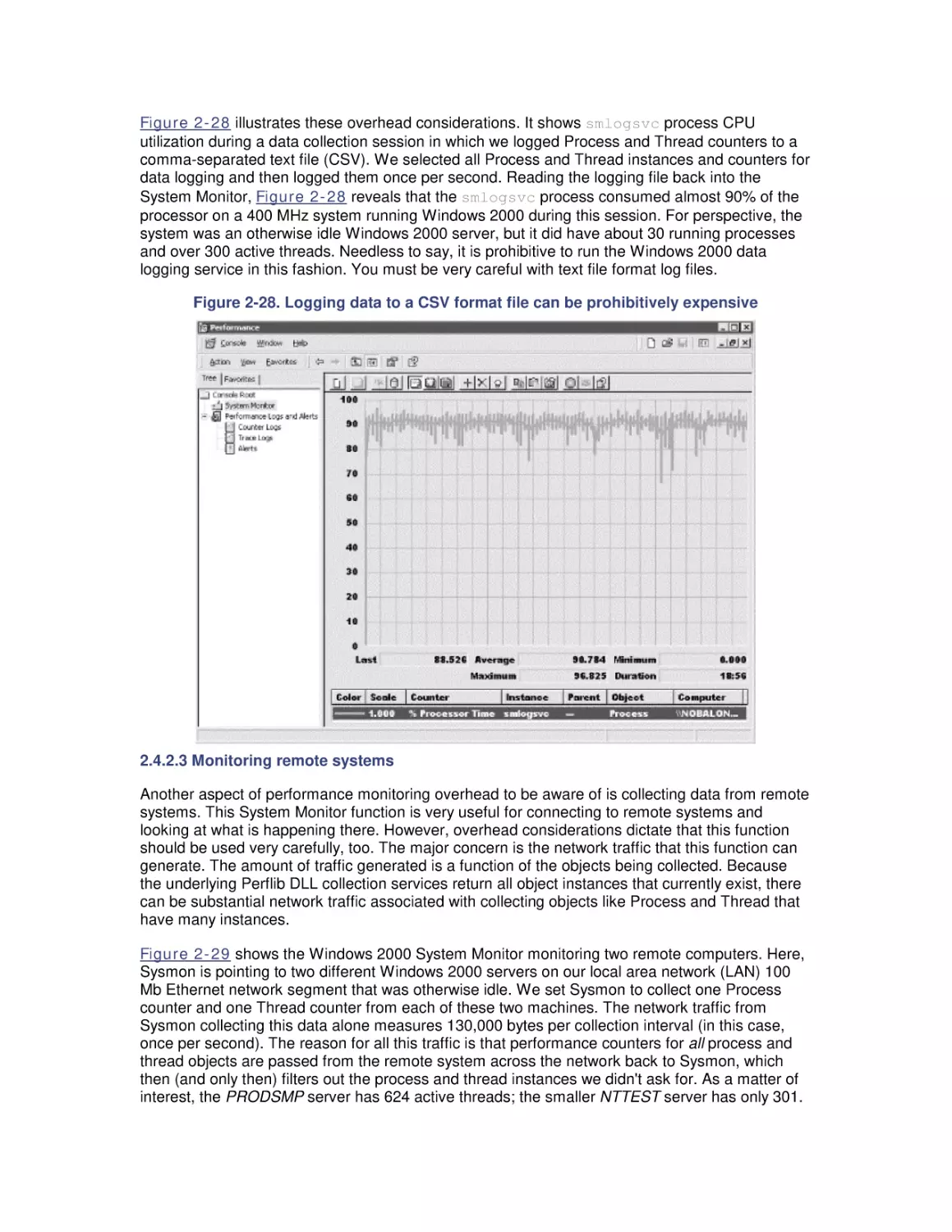
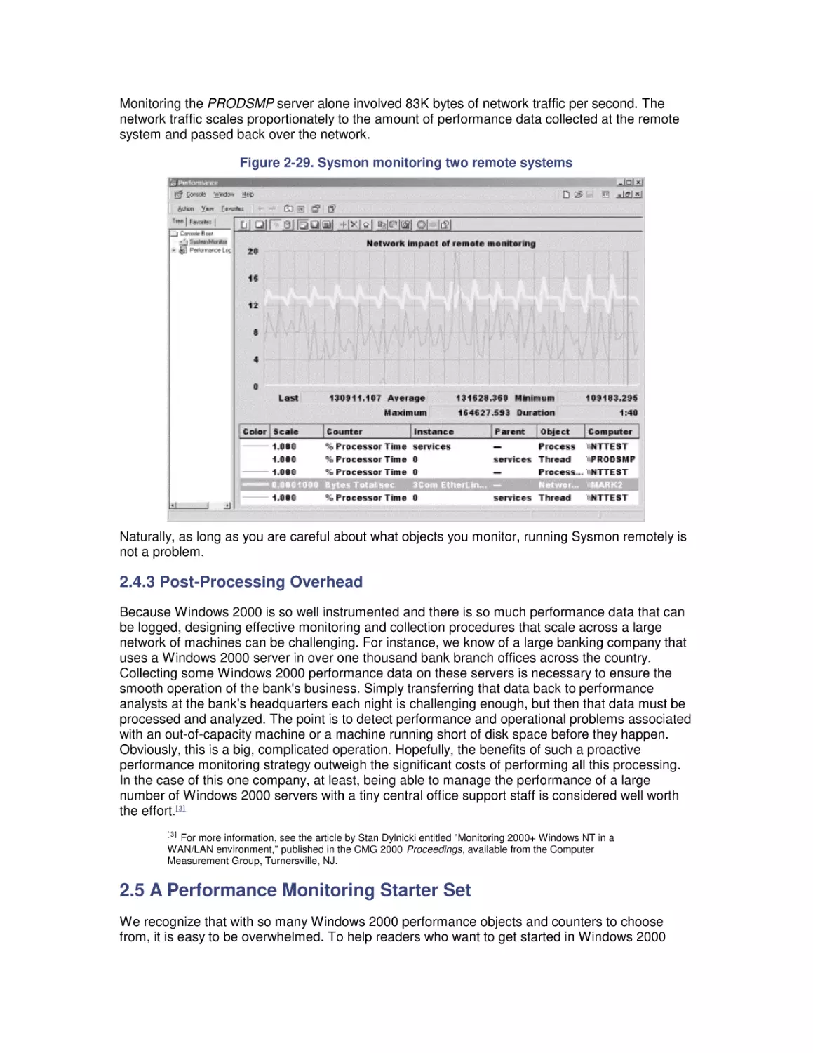
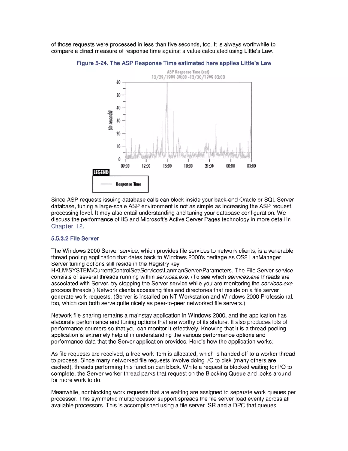
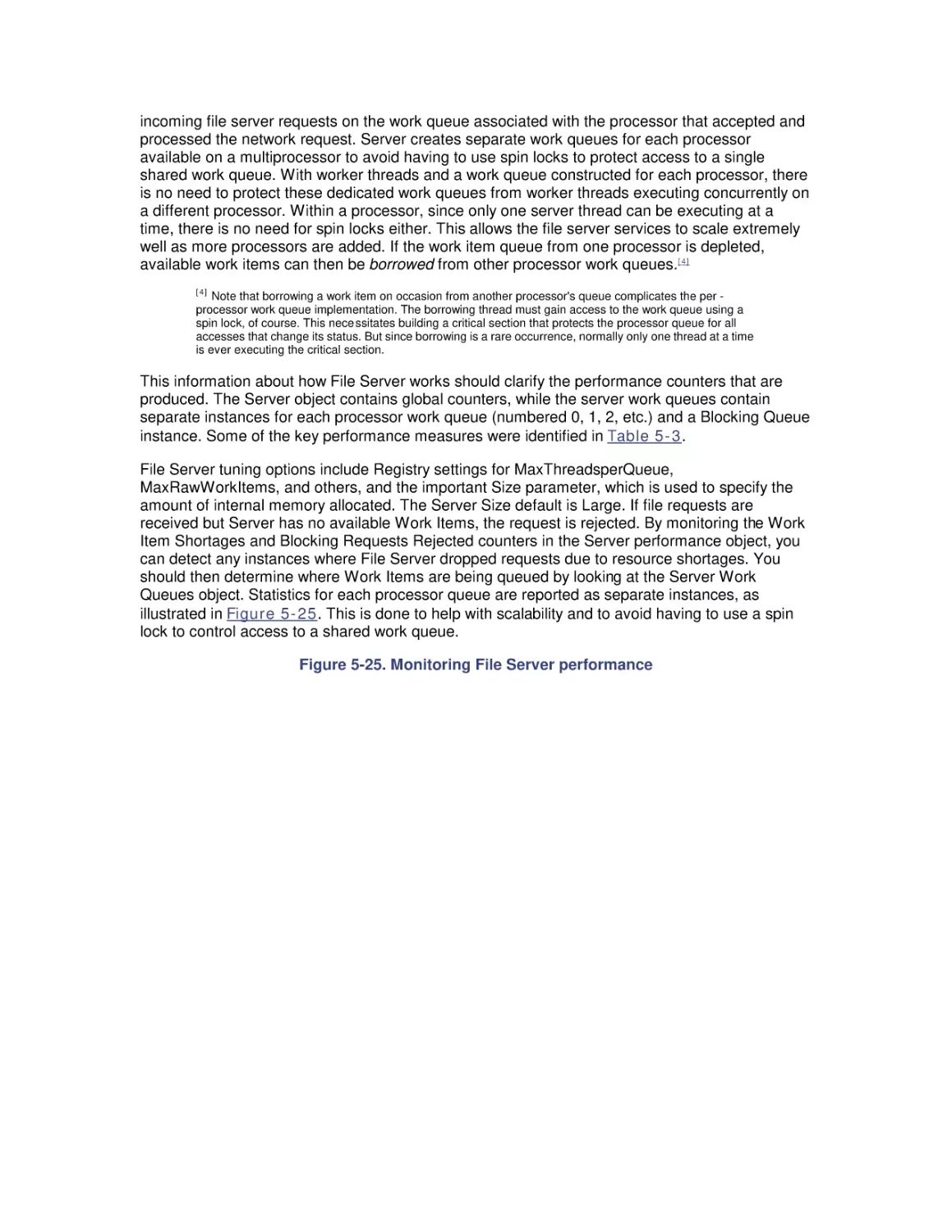
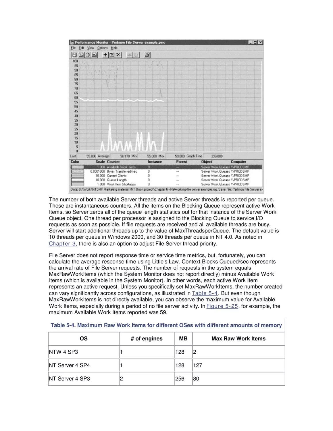
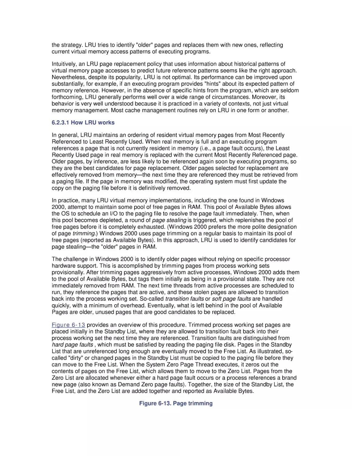
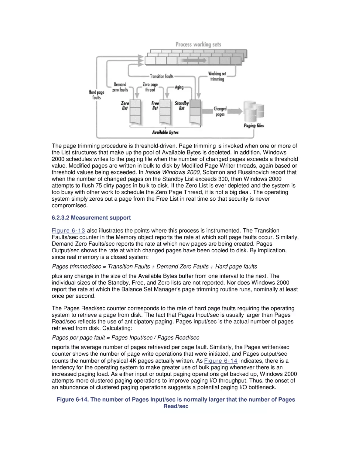
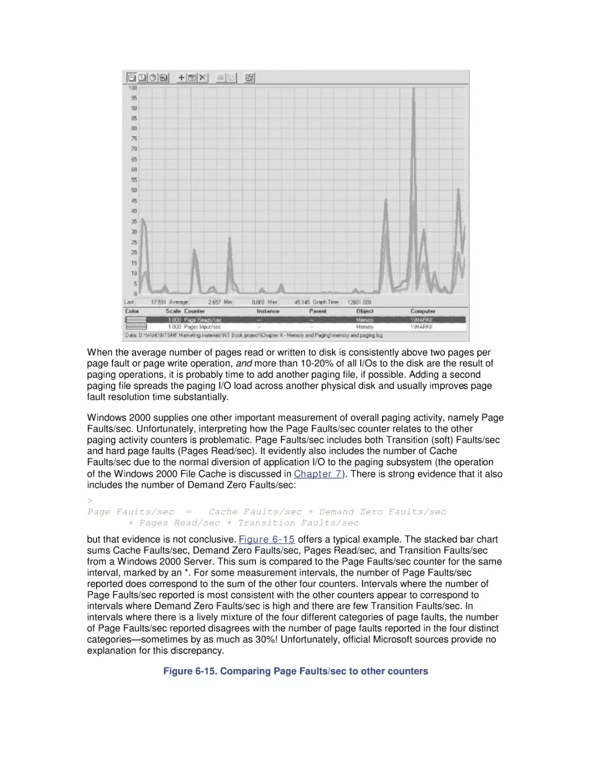
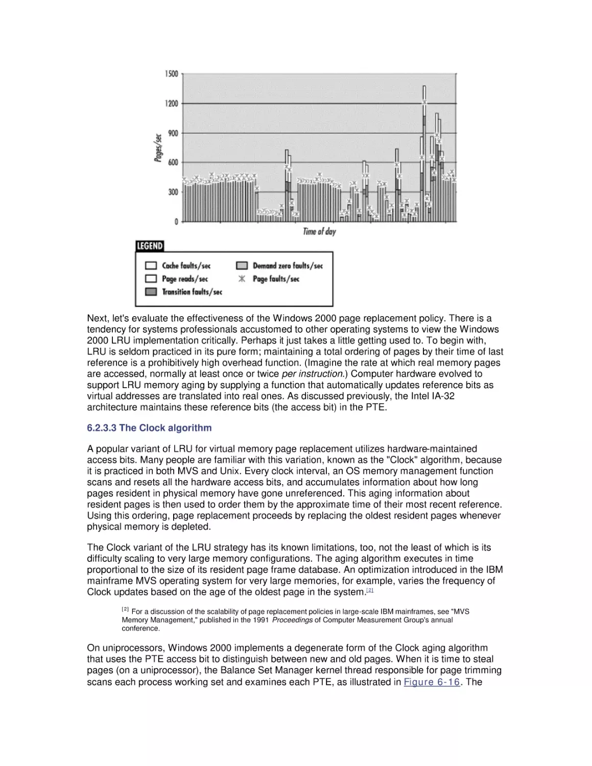
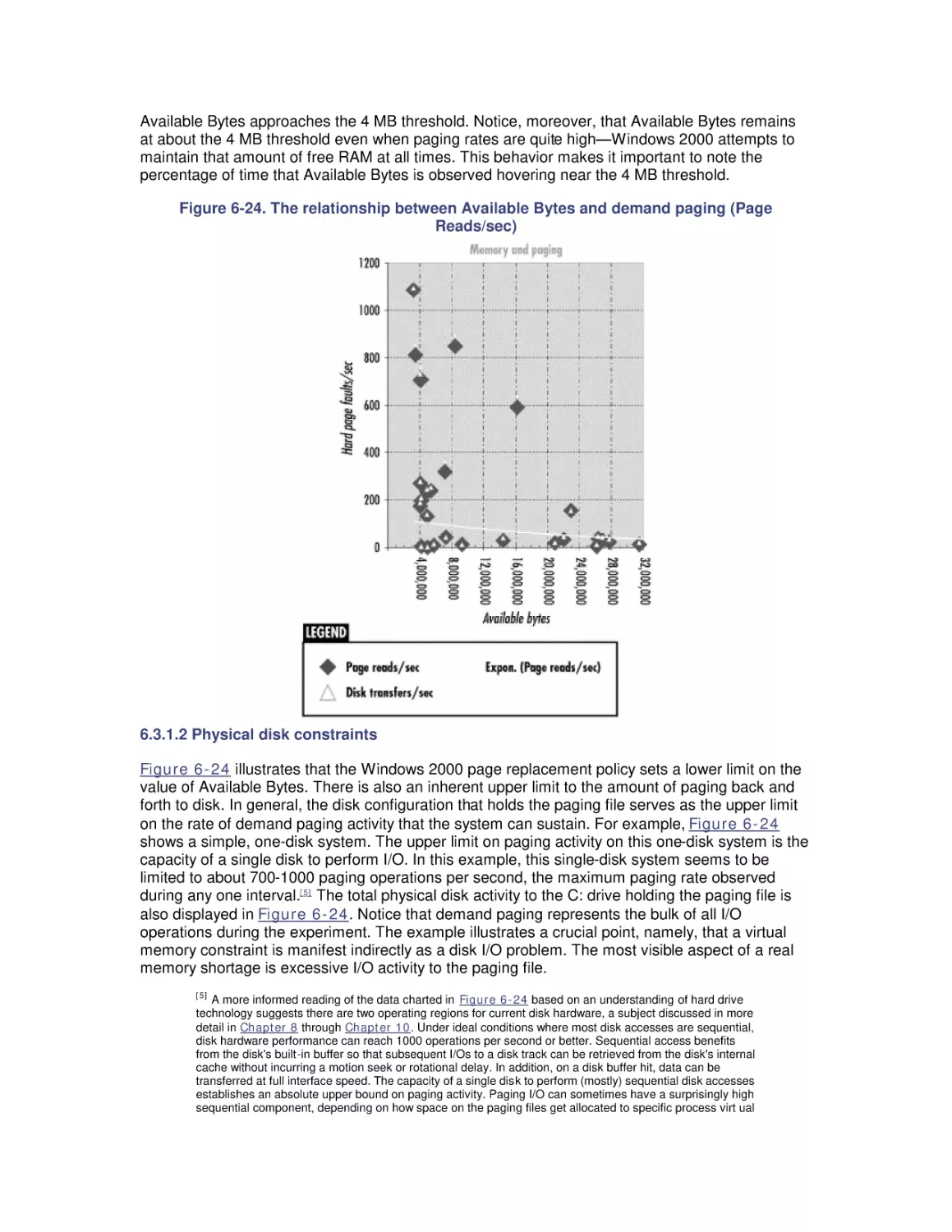
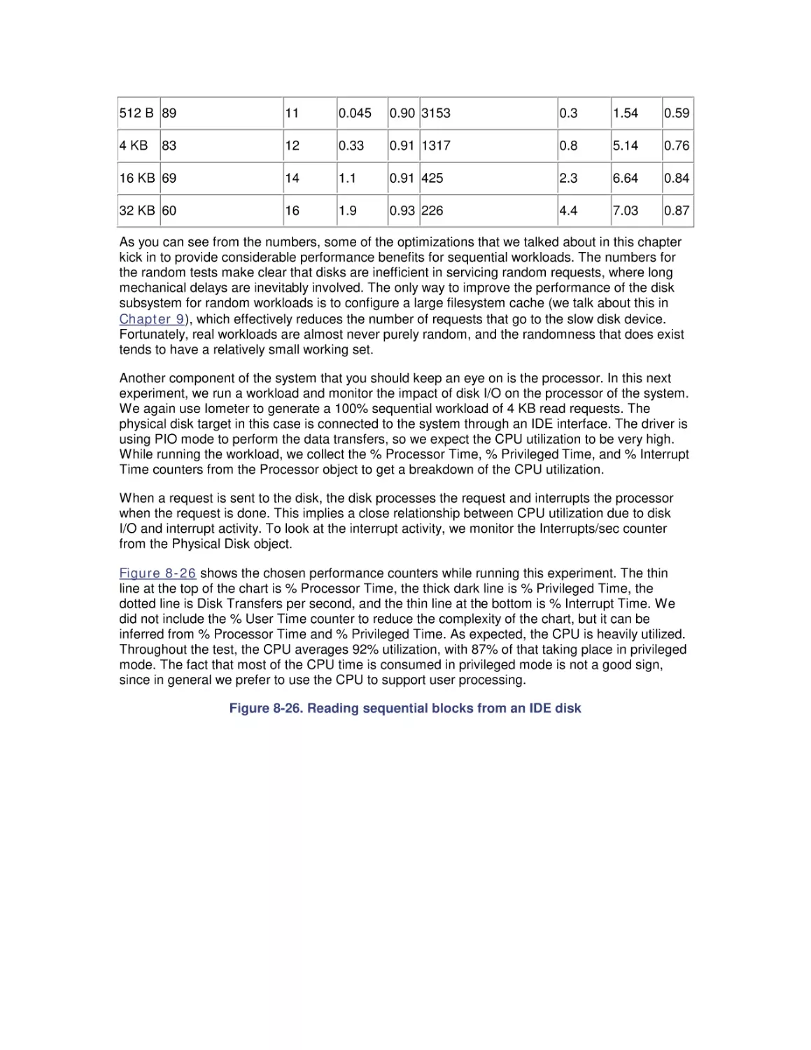
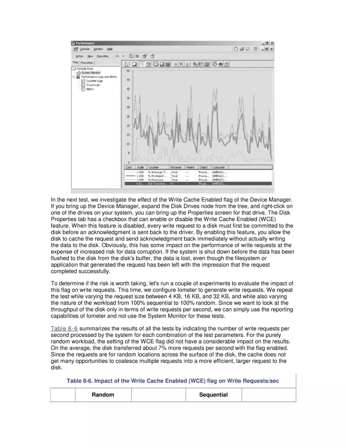
/


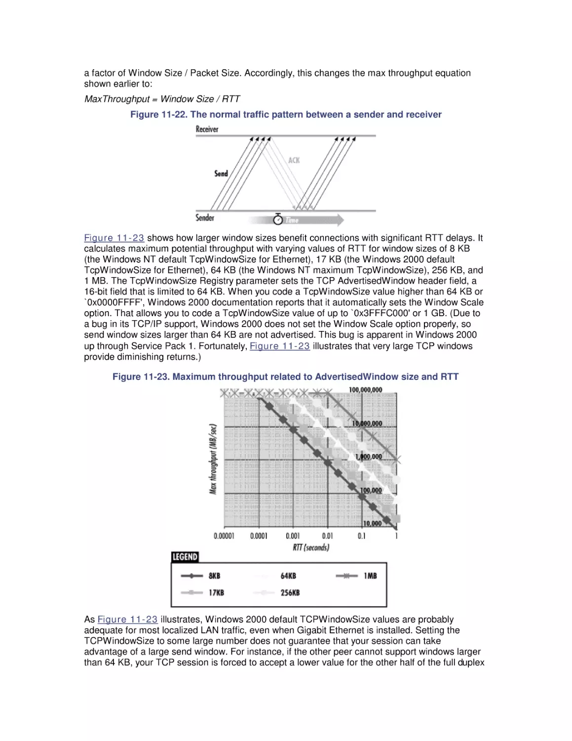


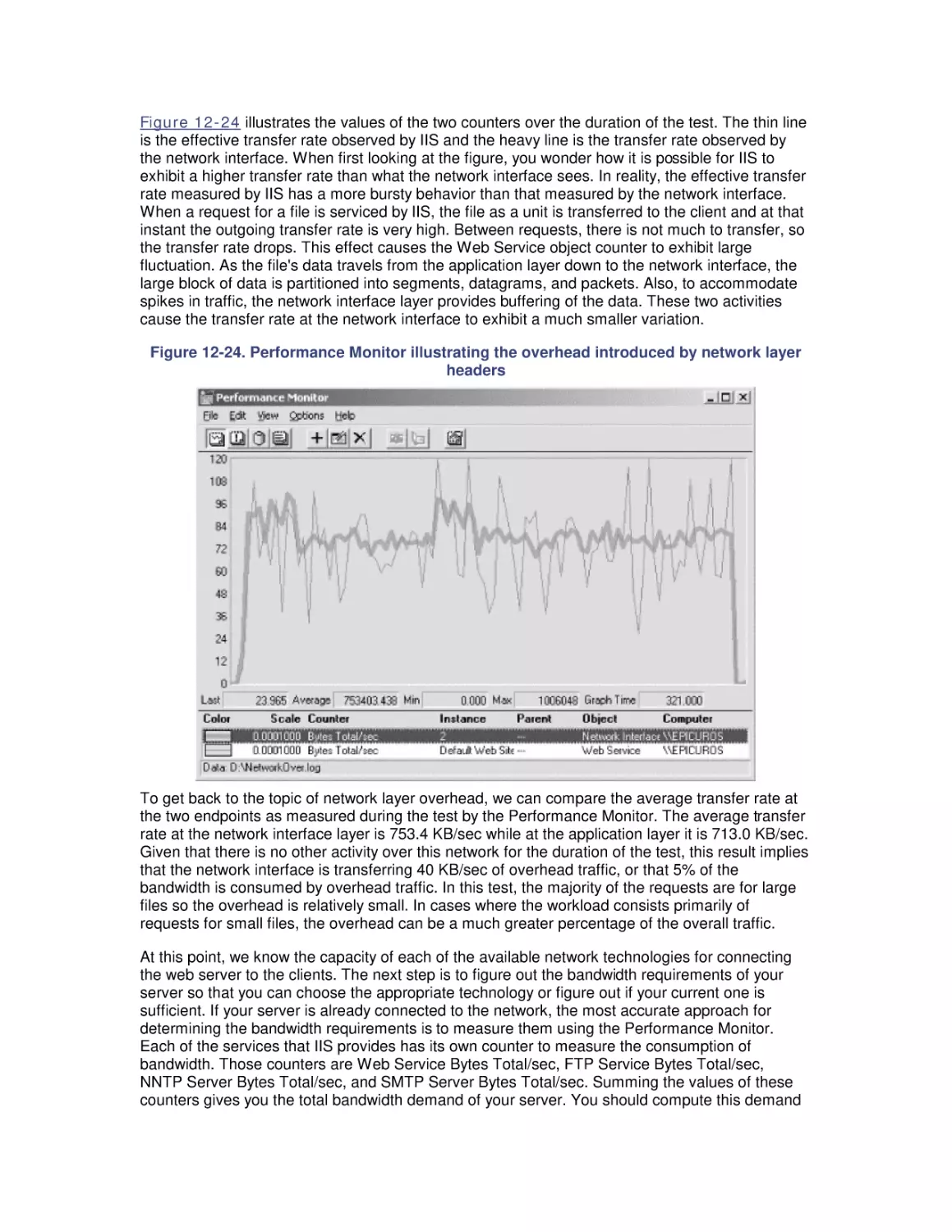


Author: Friedman Mark Pentakalos Odysseas
Tags: windows operating system
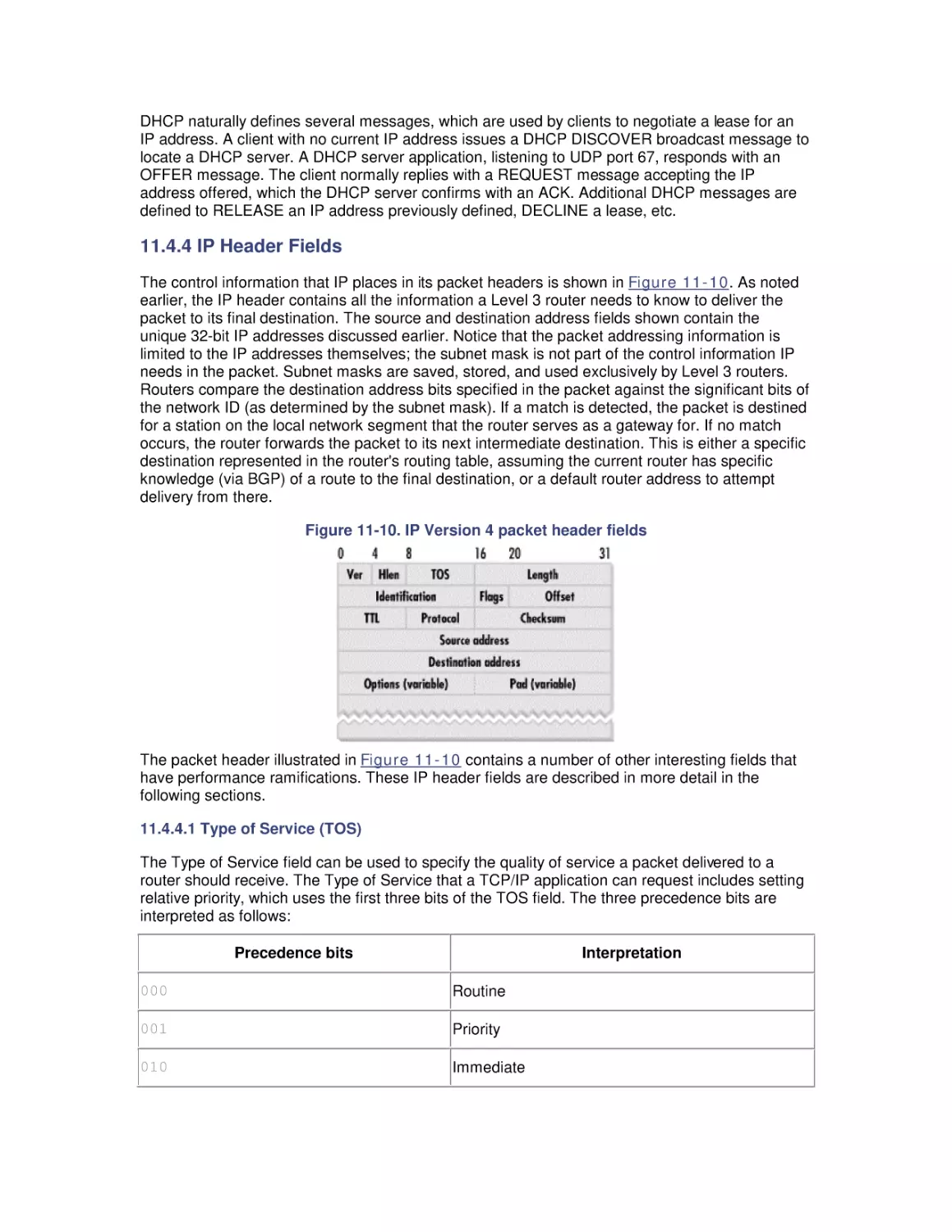
ISBN: 1-56592-466-5
Year: 2002


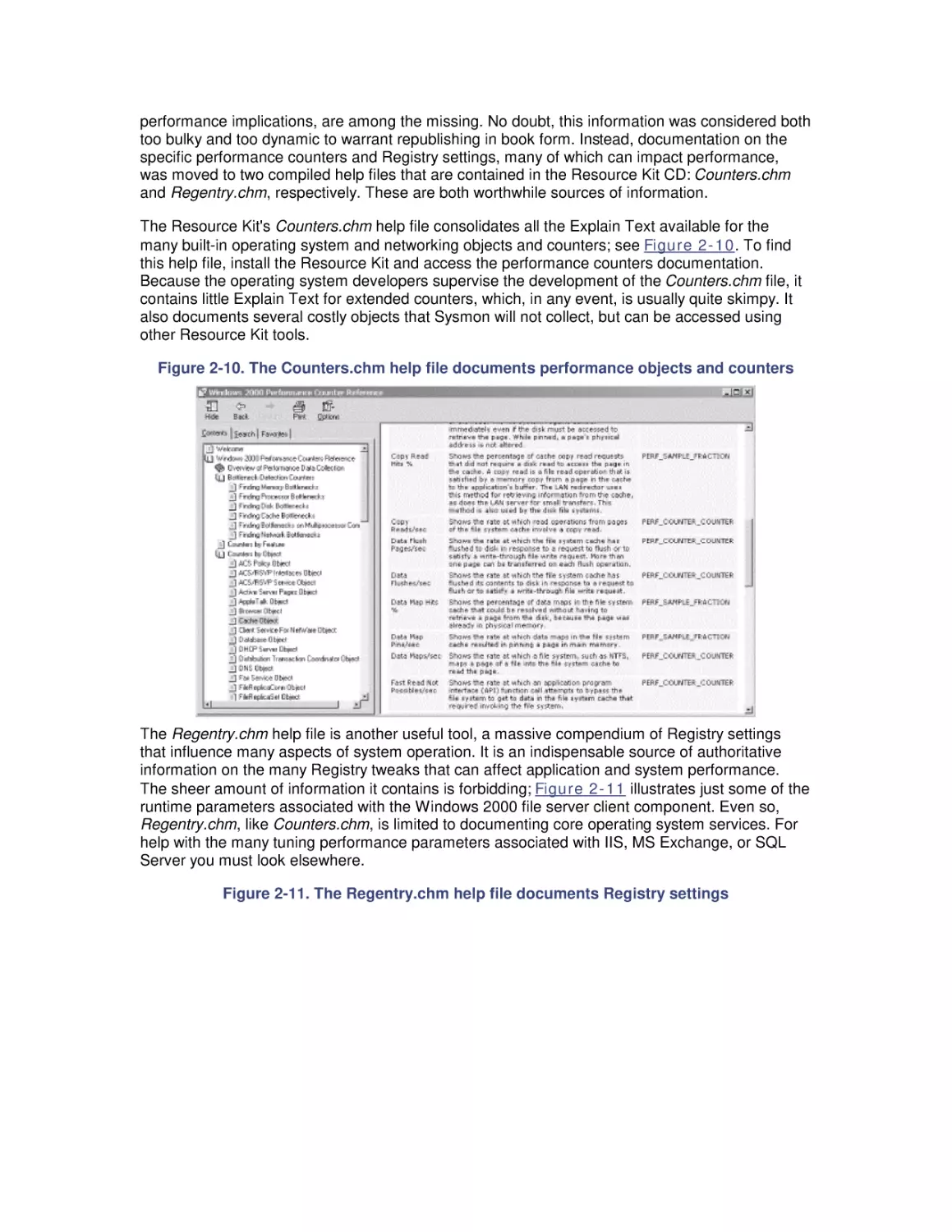
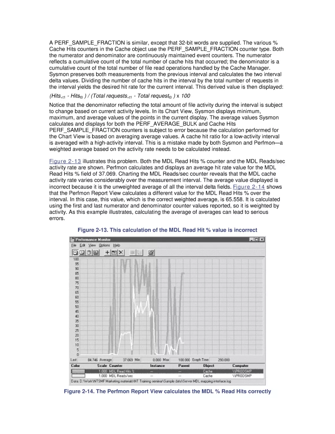
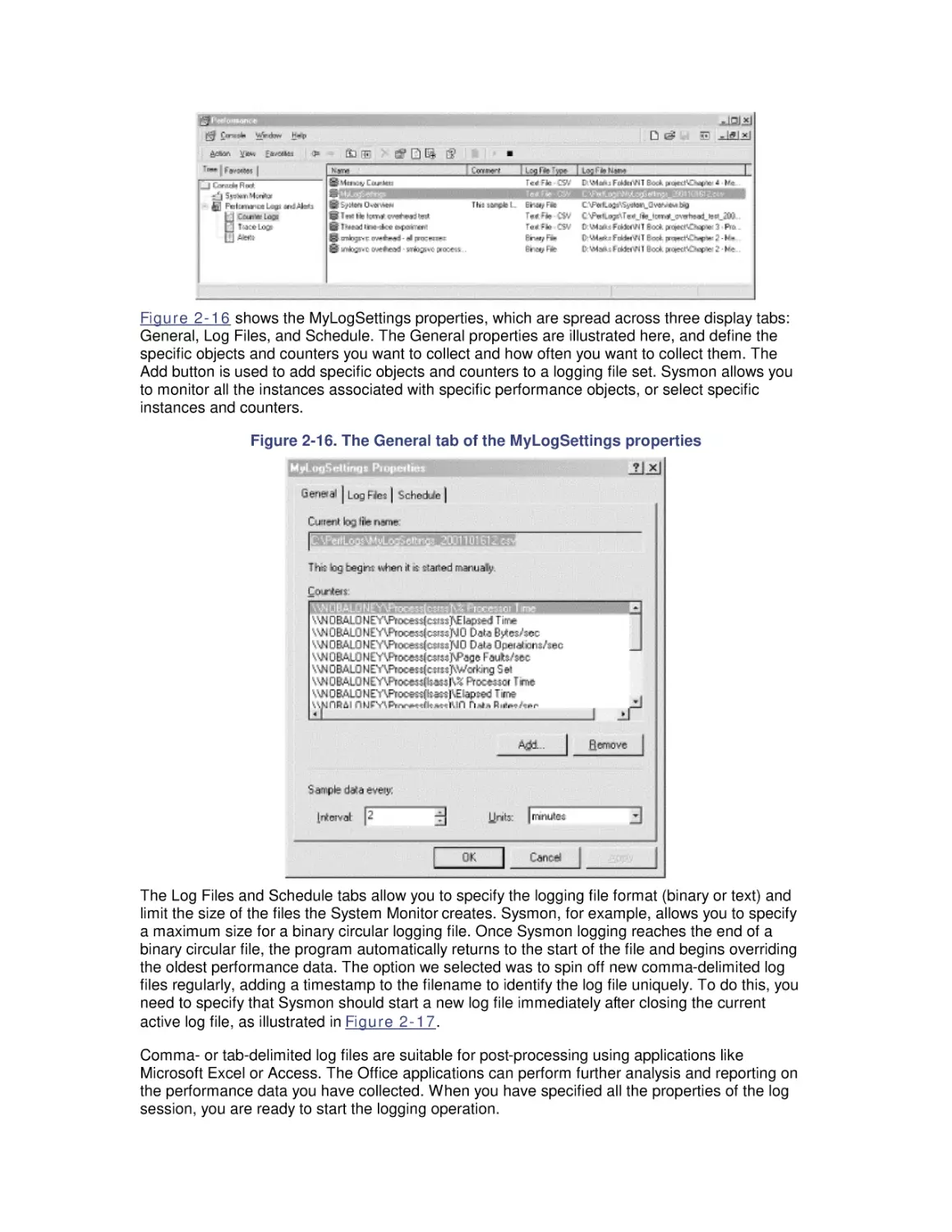
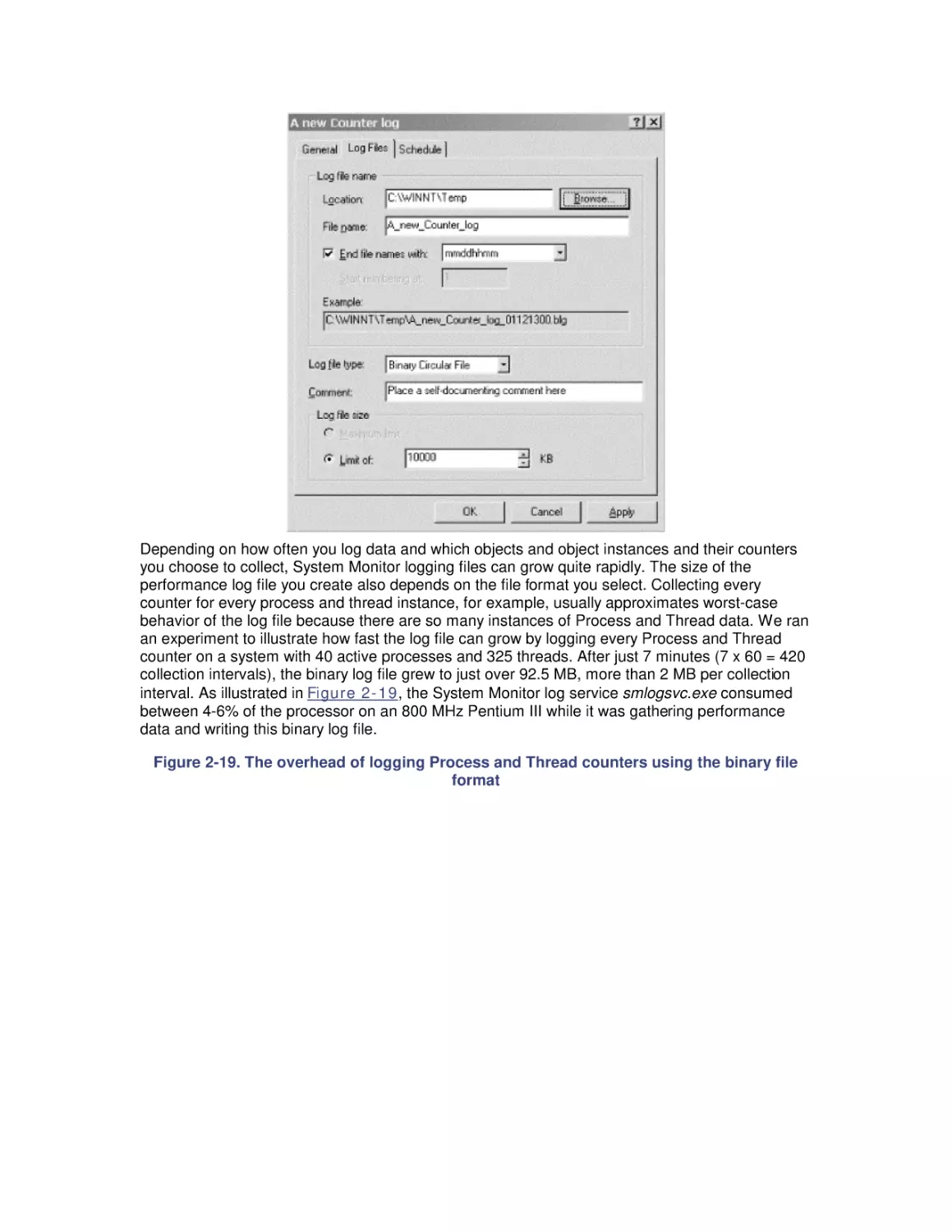
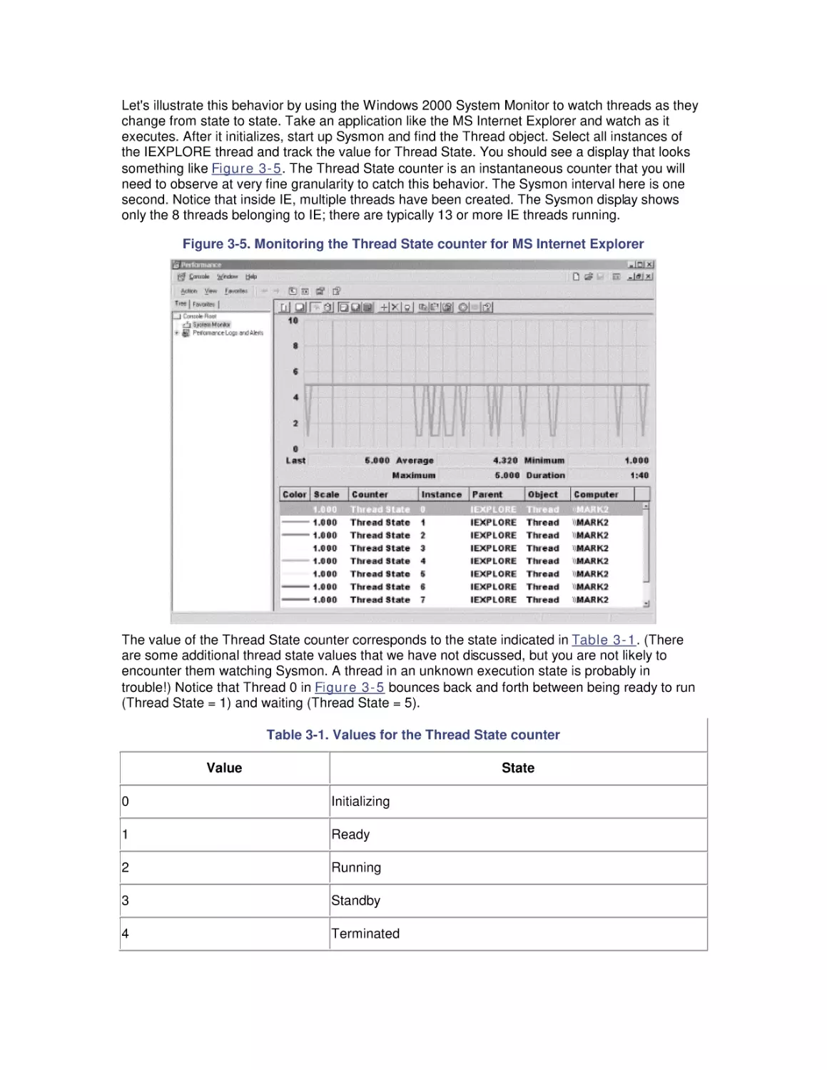
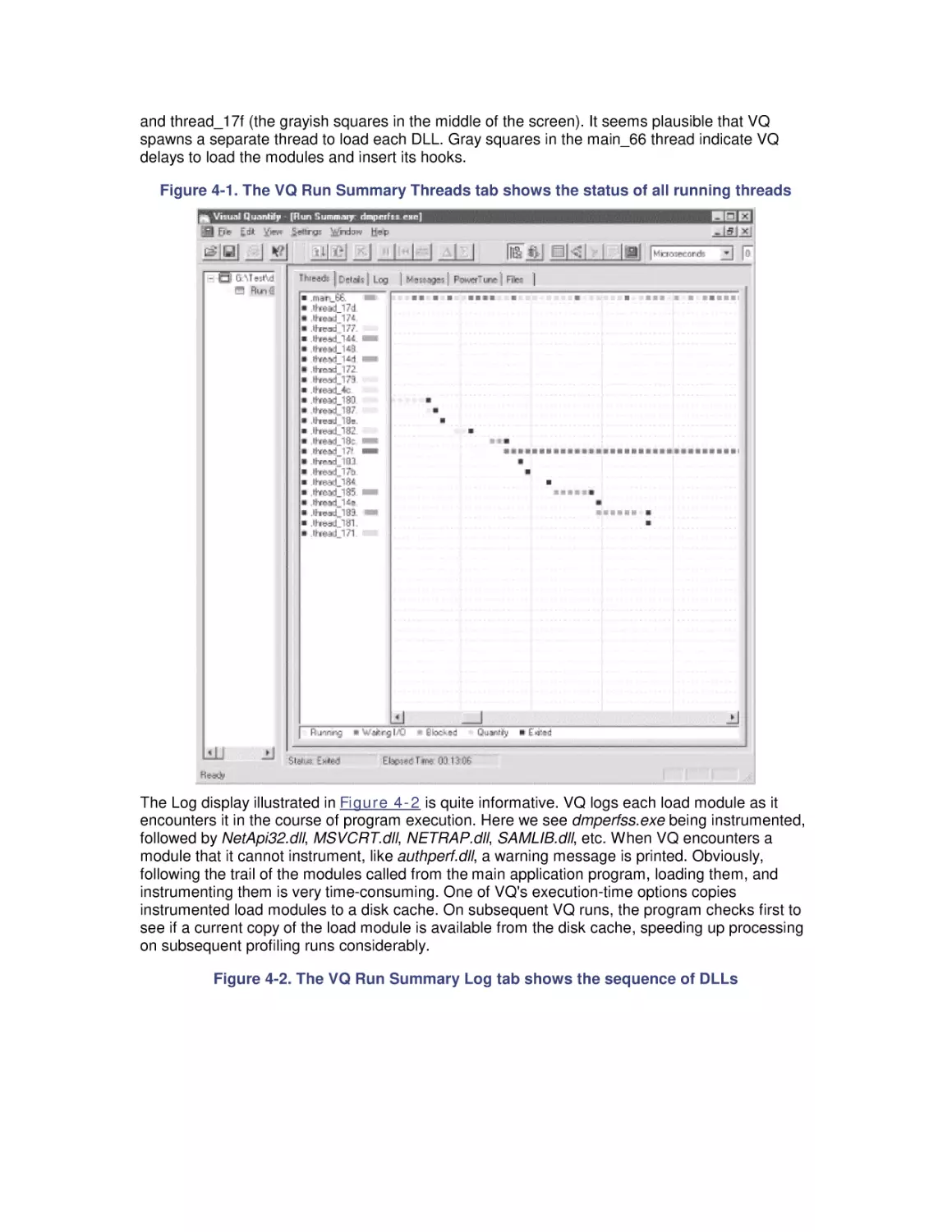
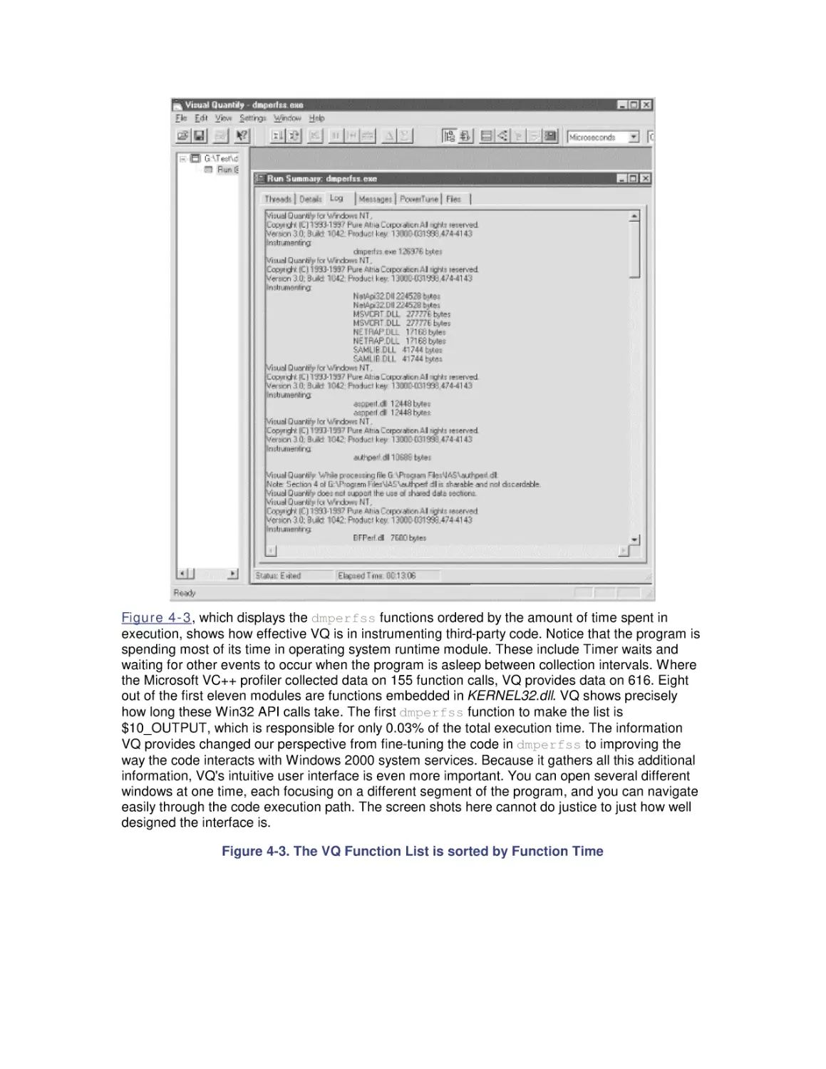
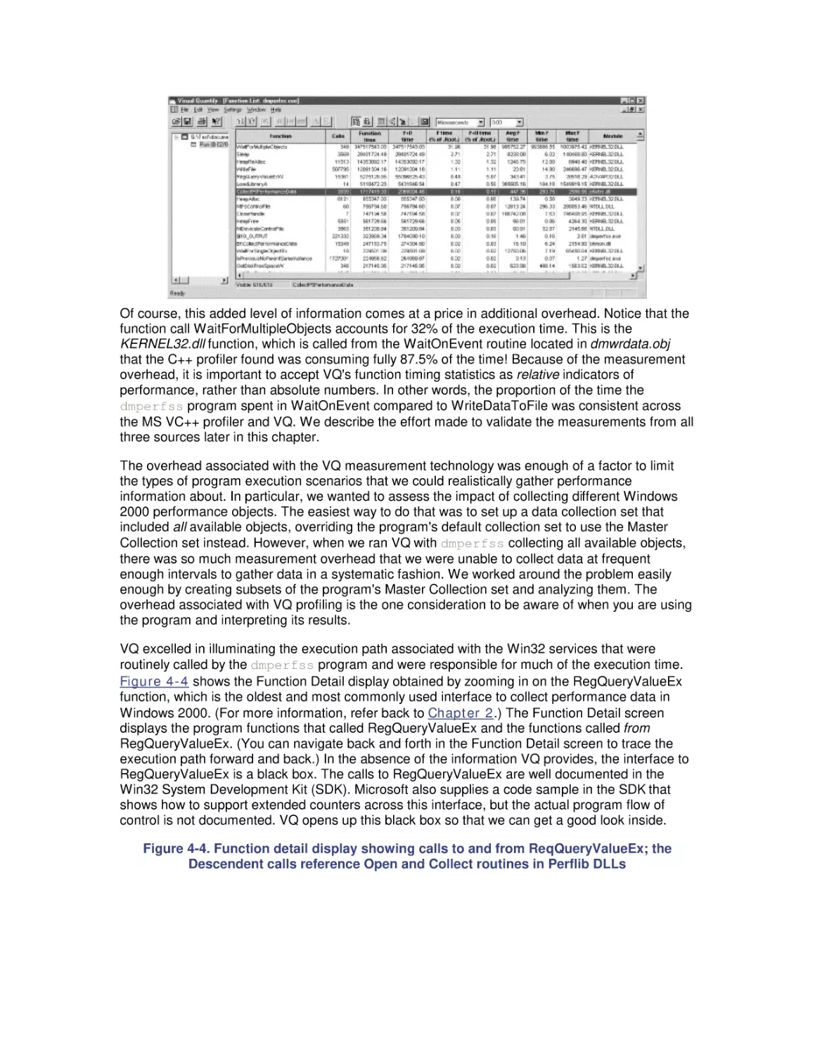
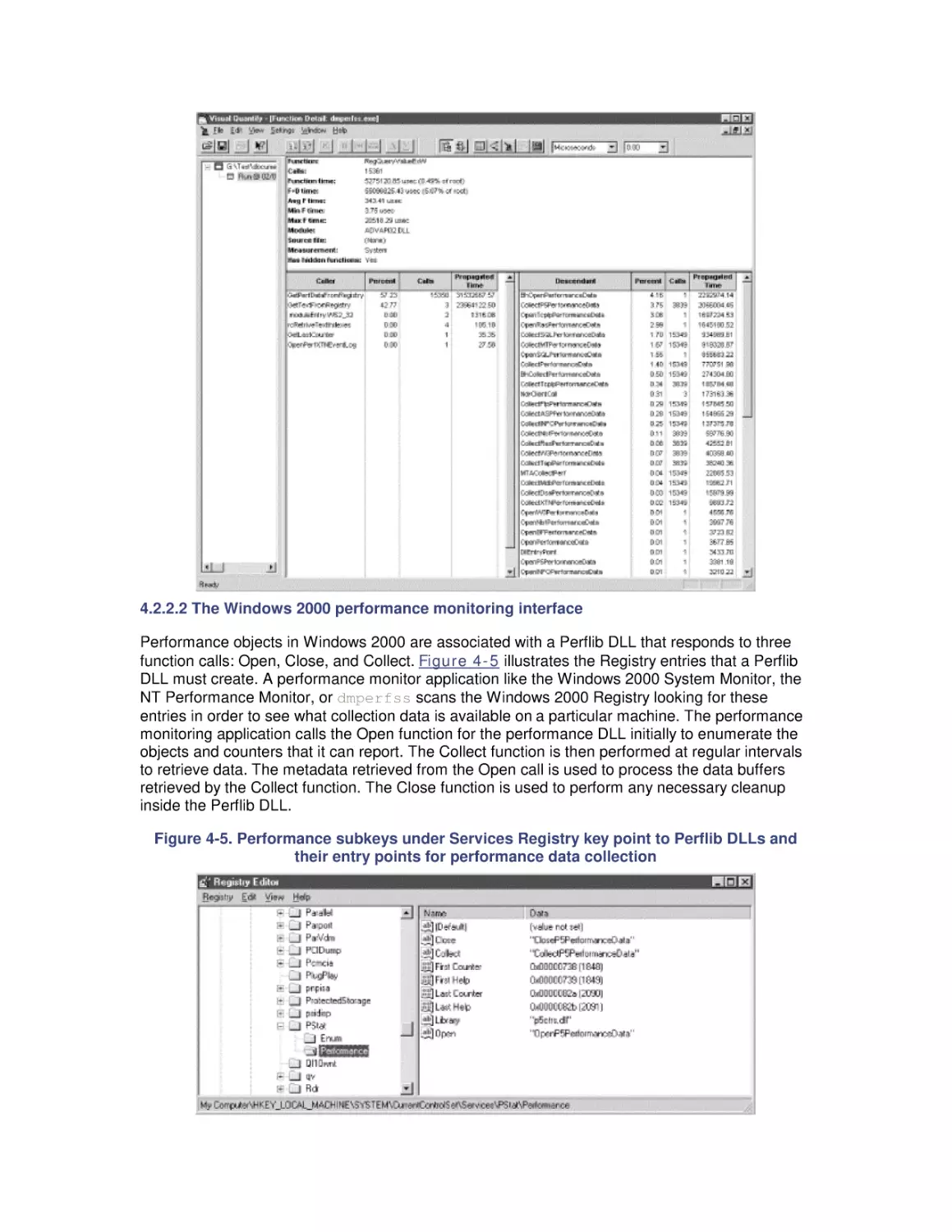
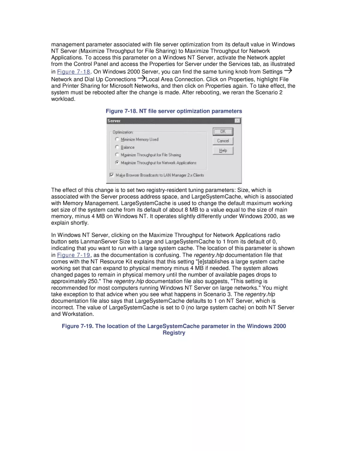
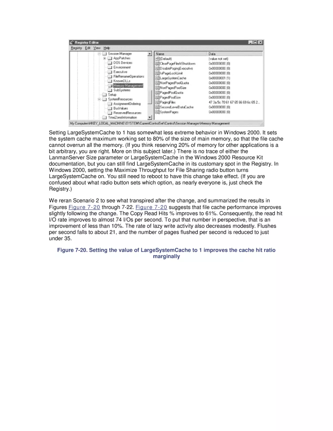
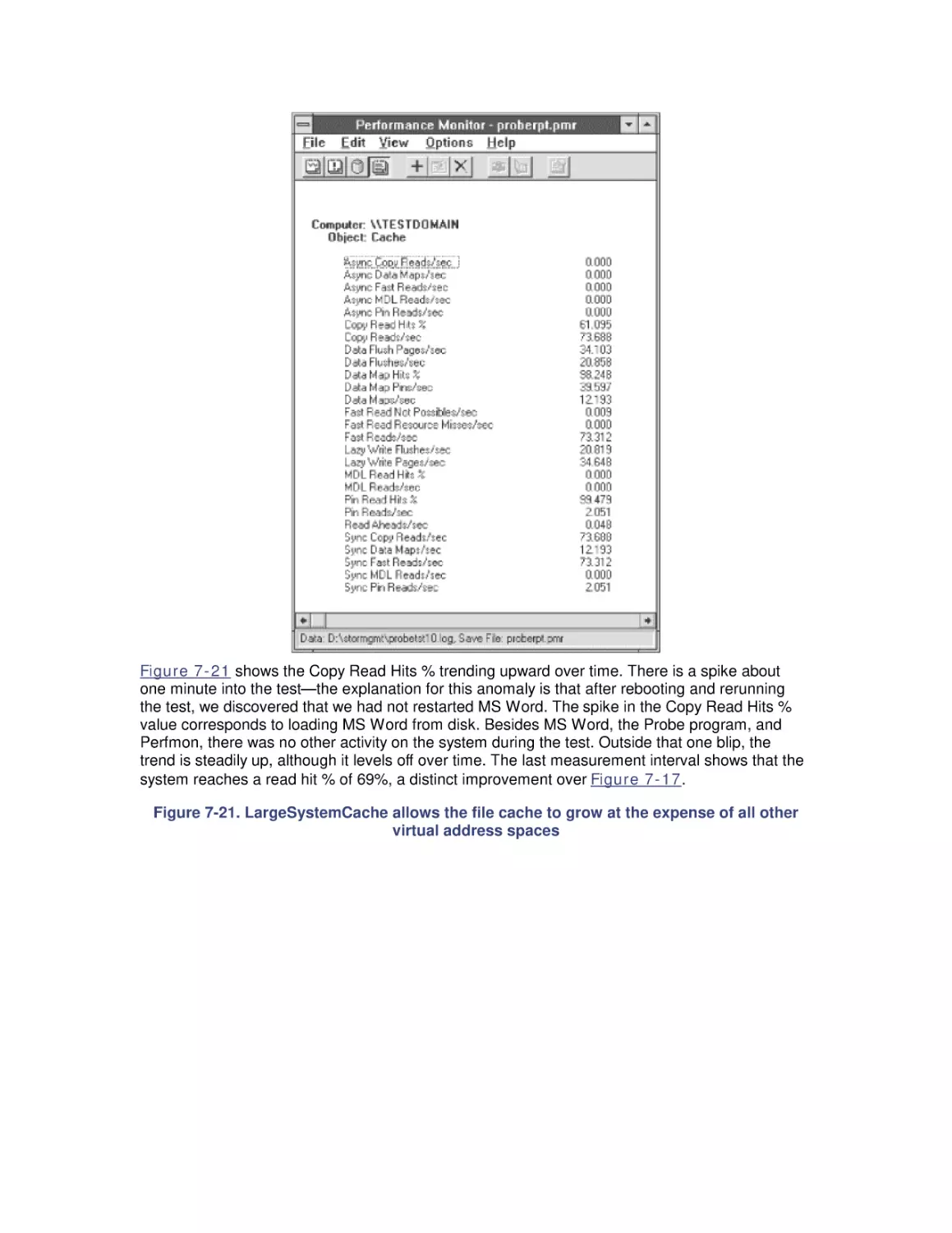
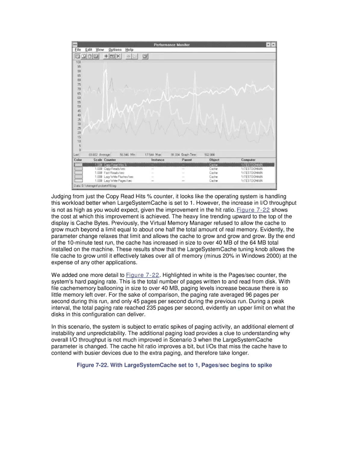
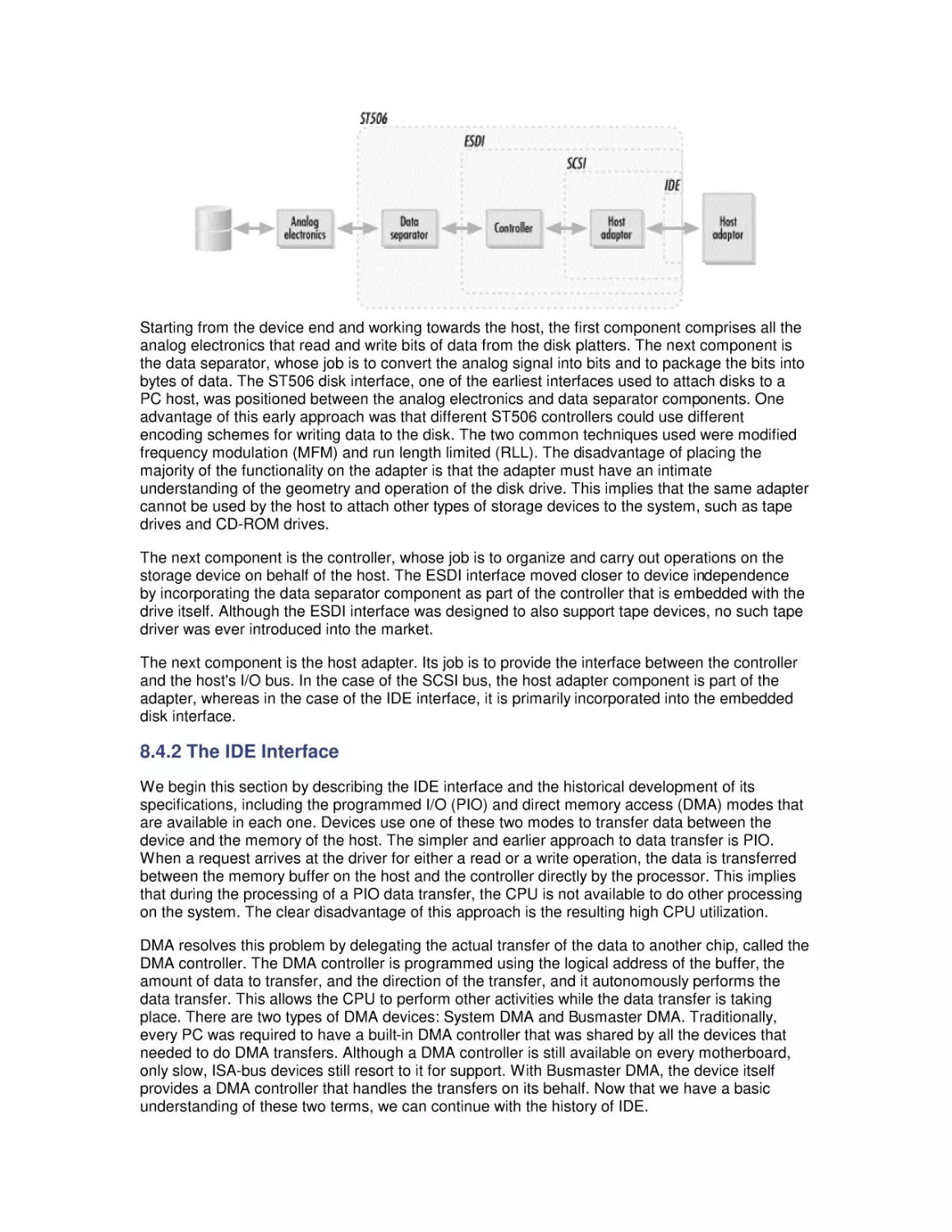
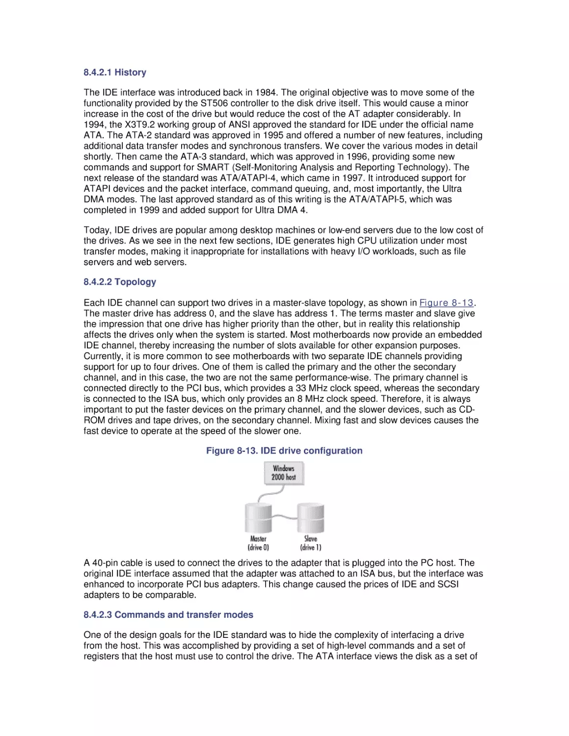
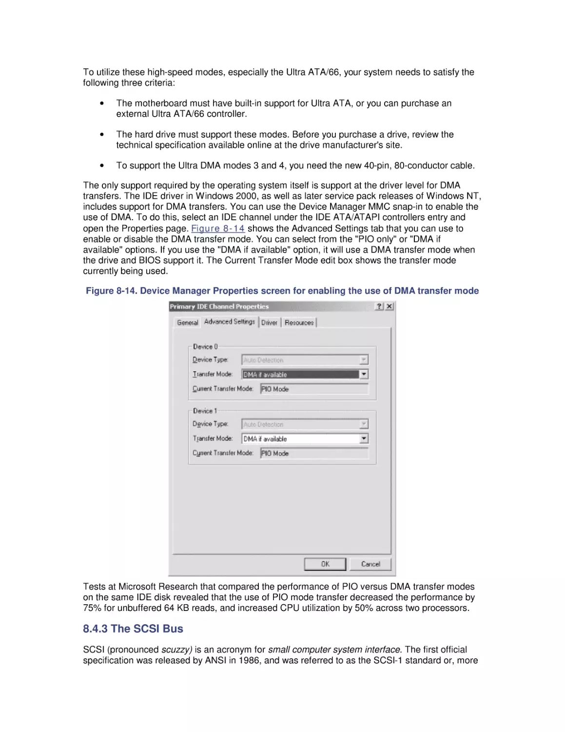
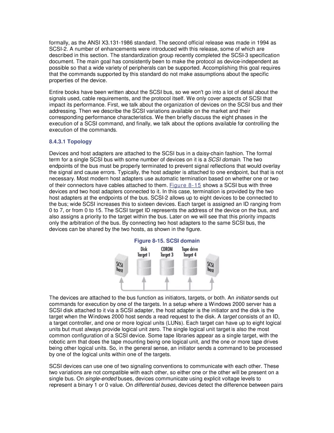
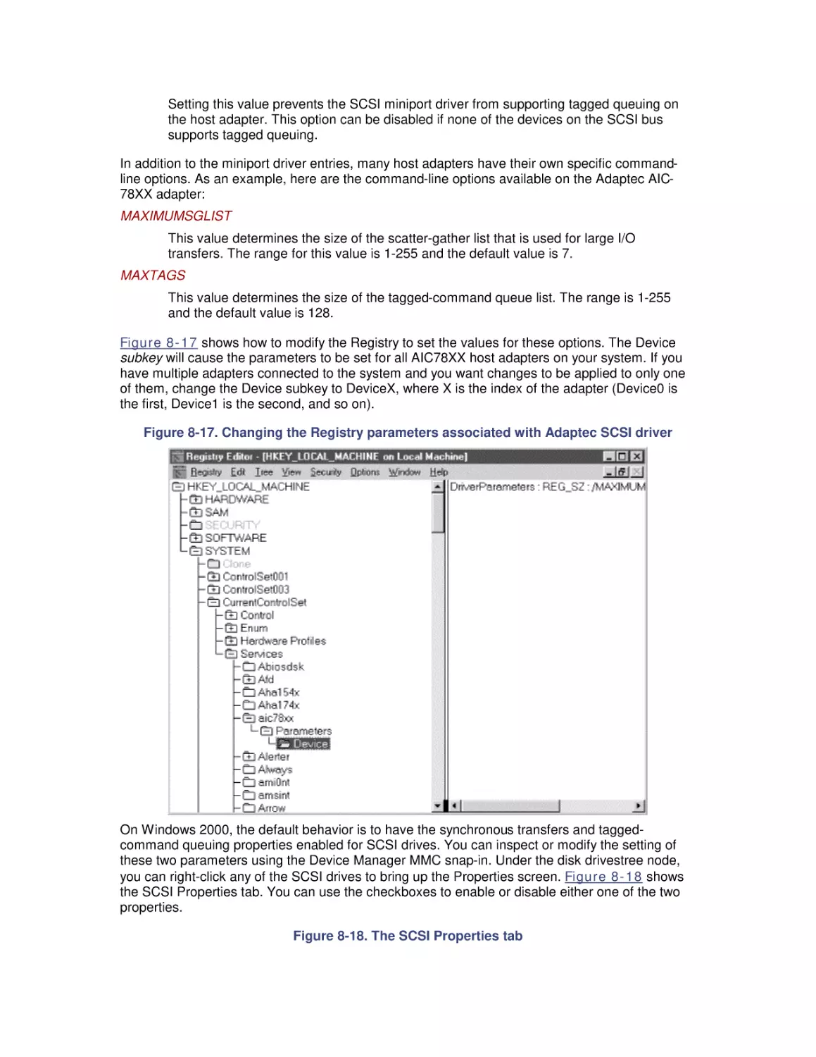
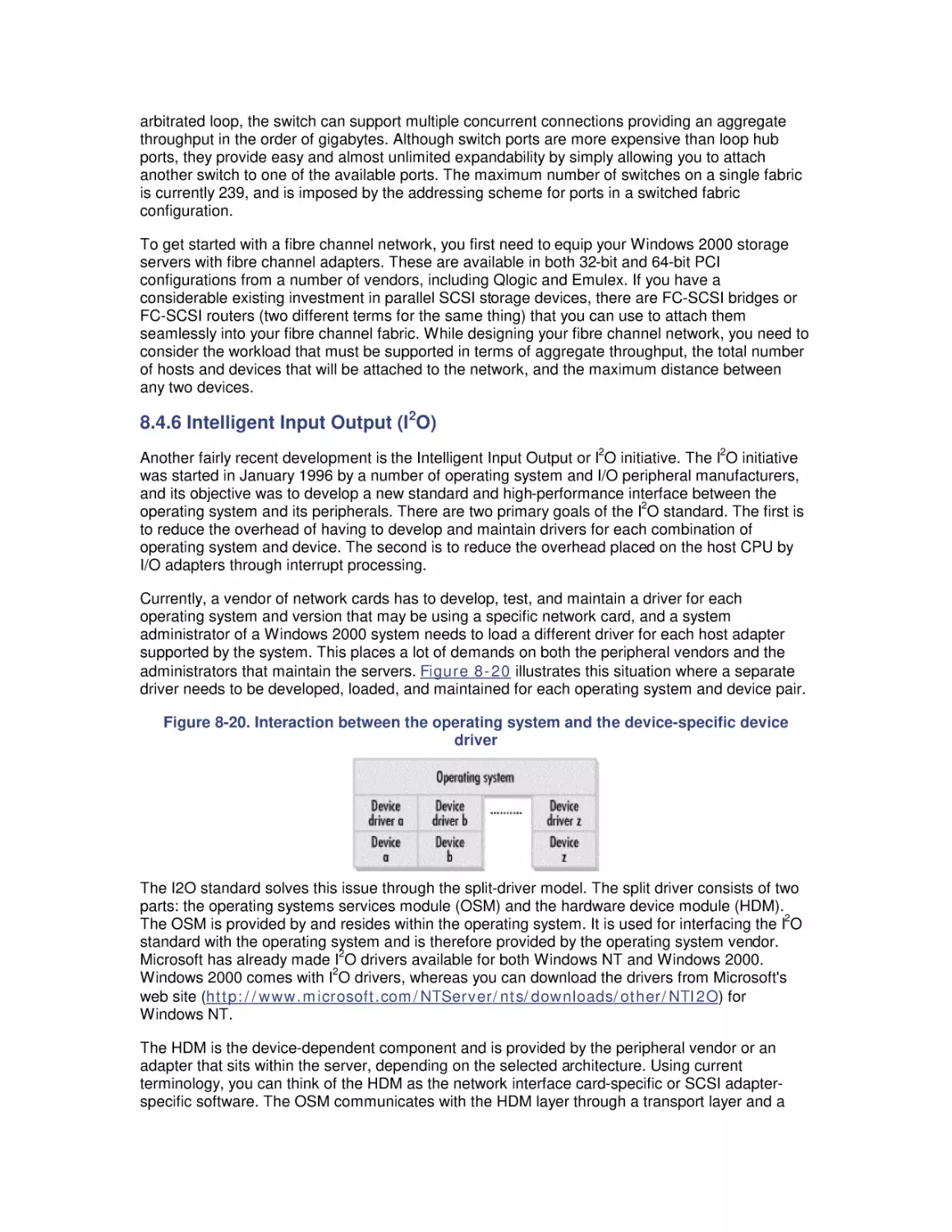
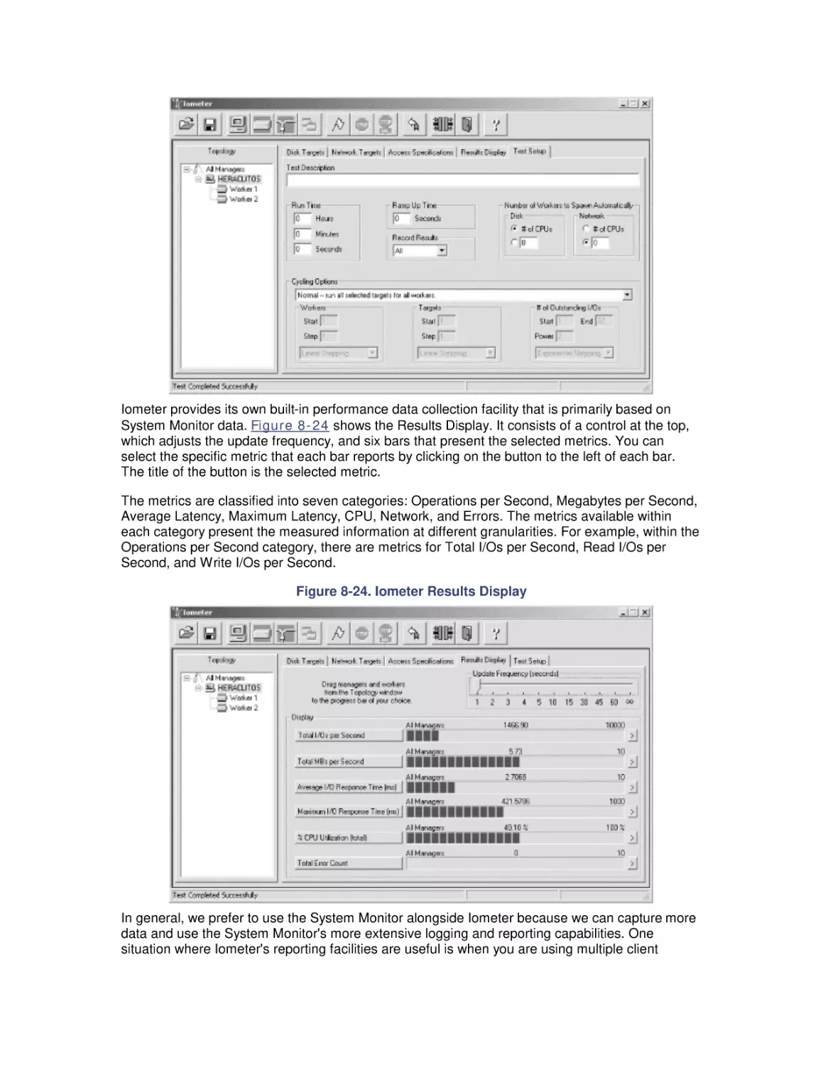
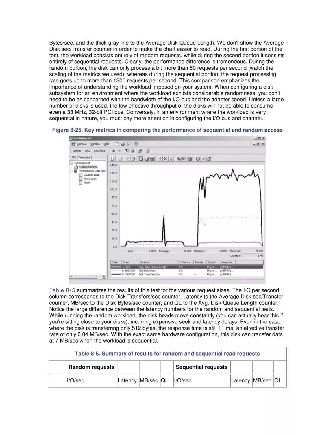
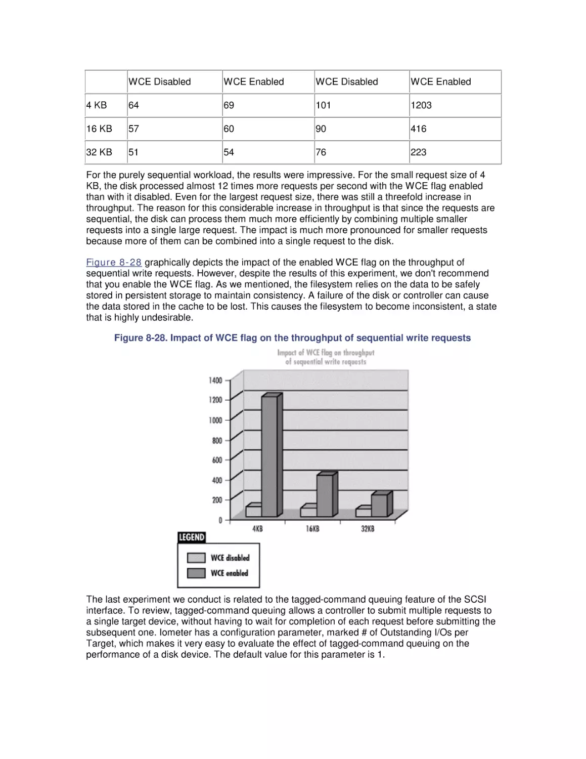
Text
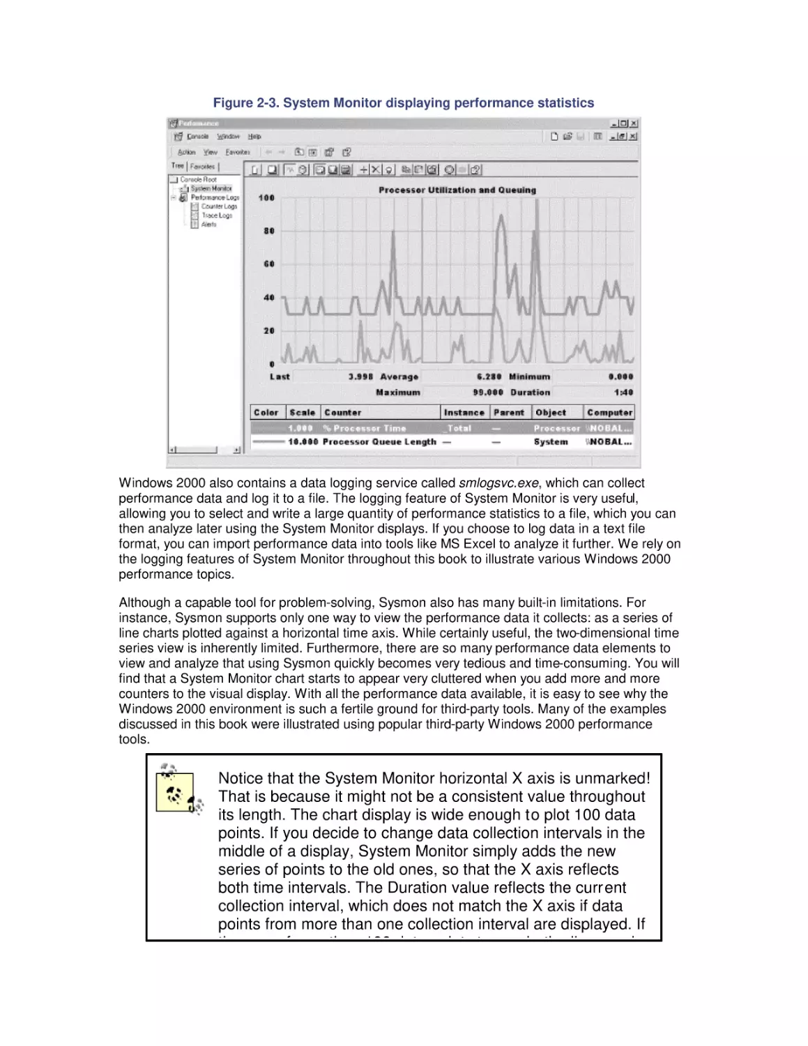
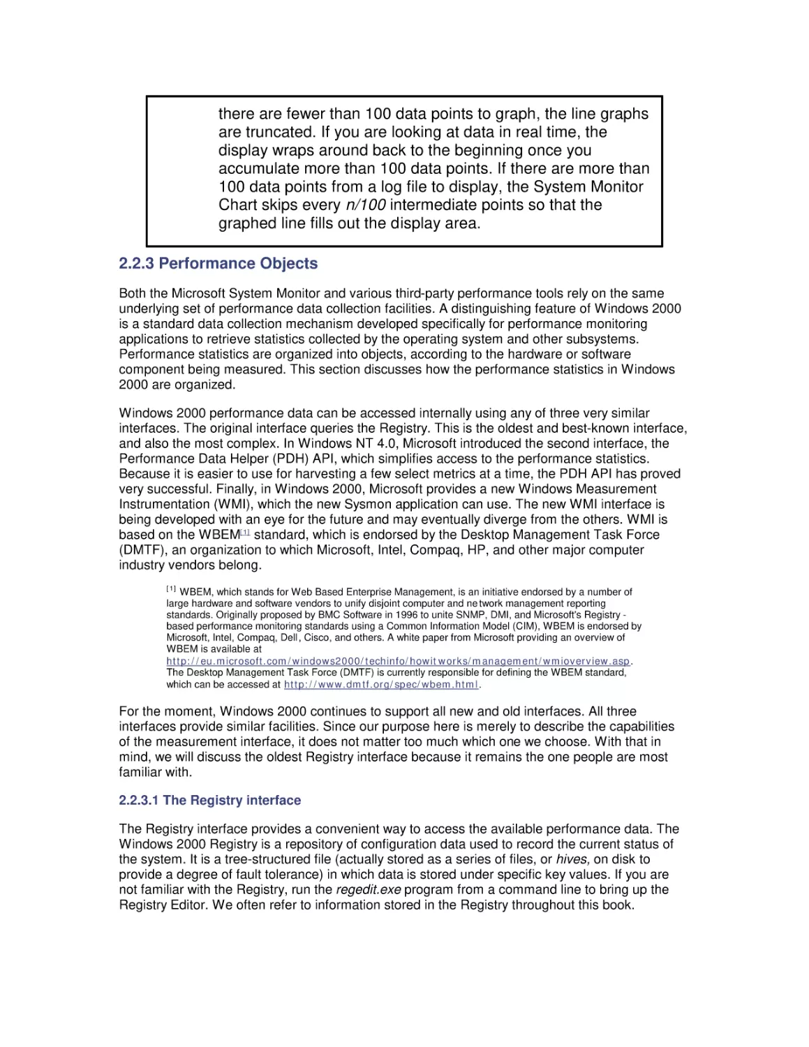
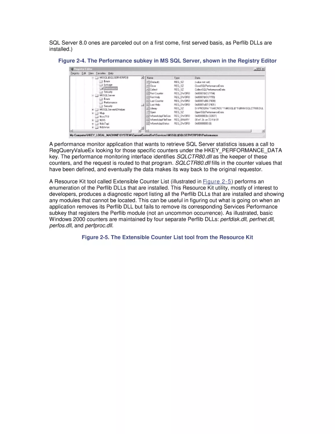
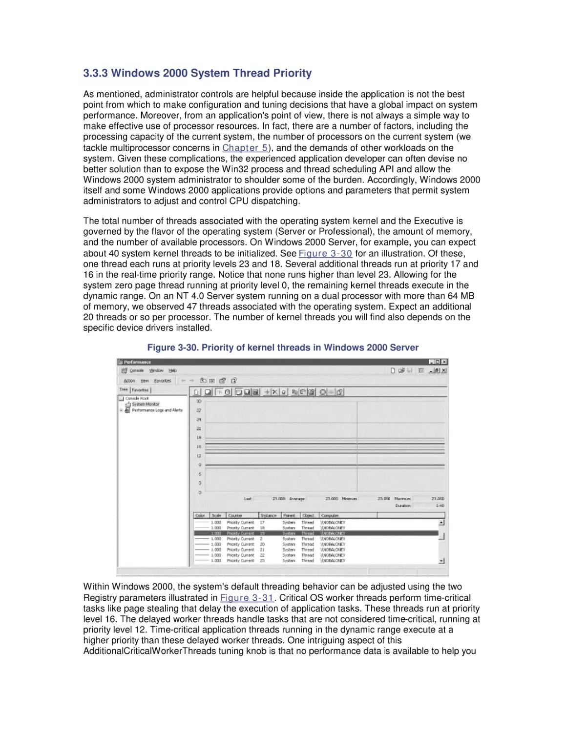
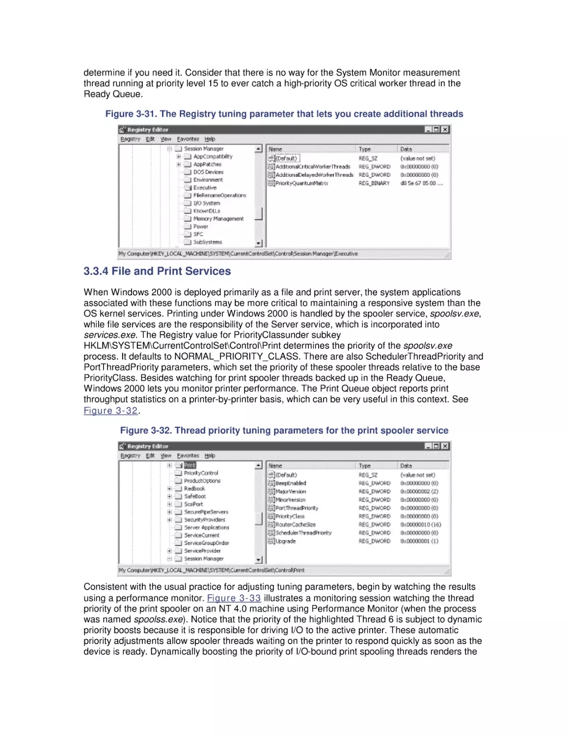
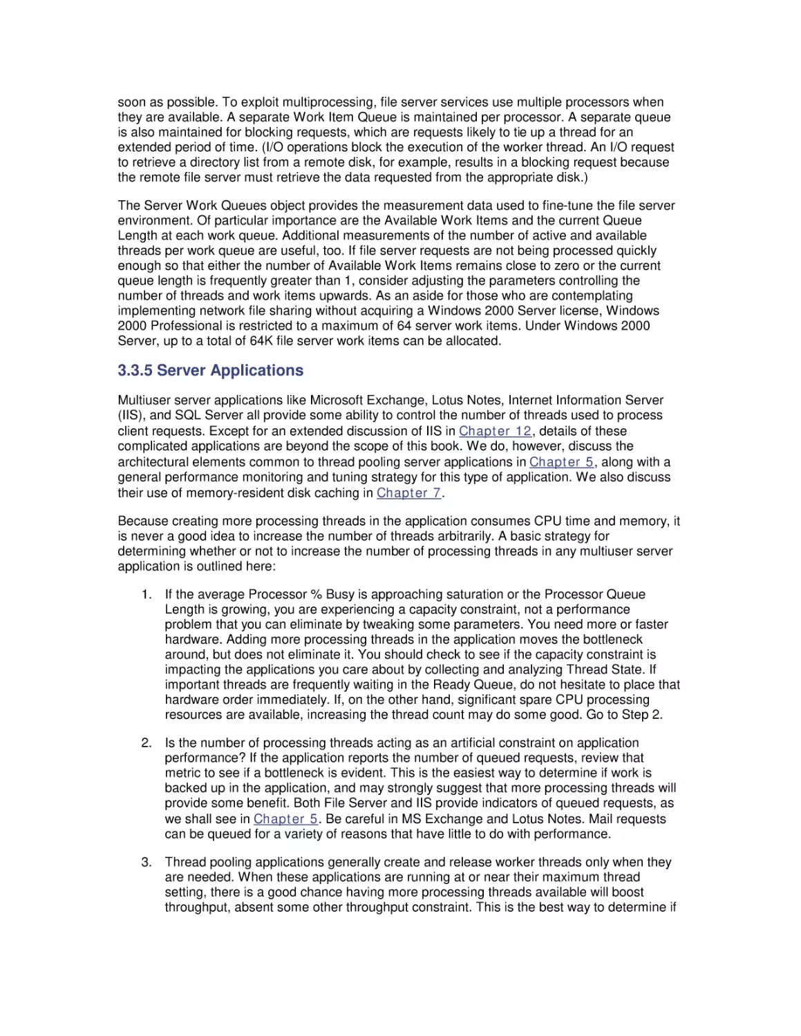
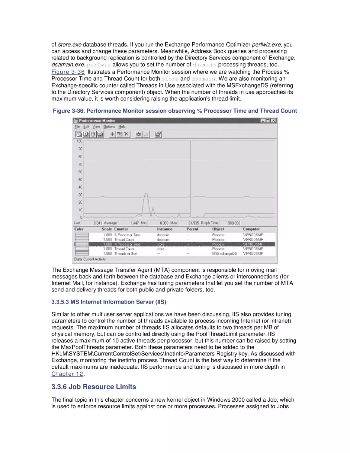
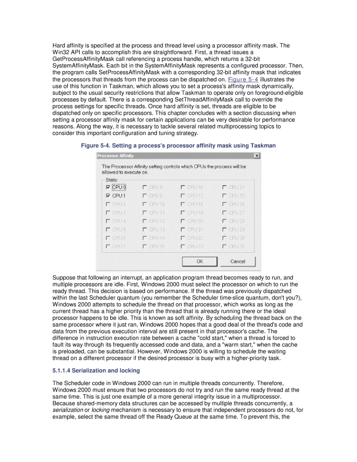
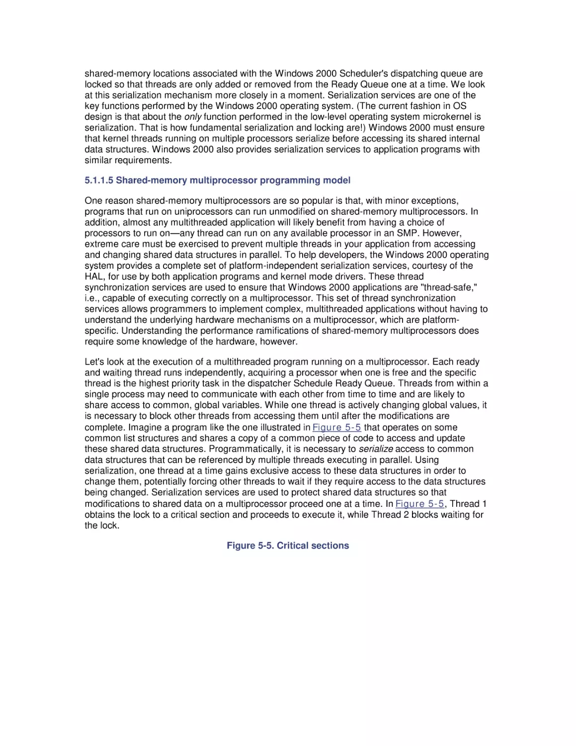
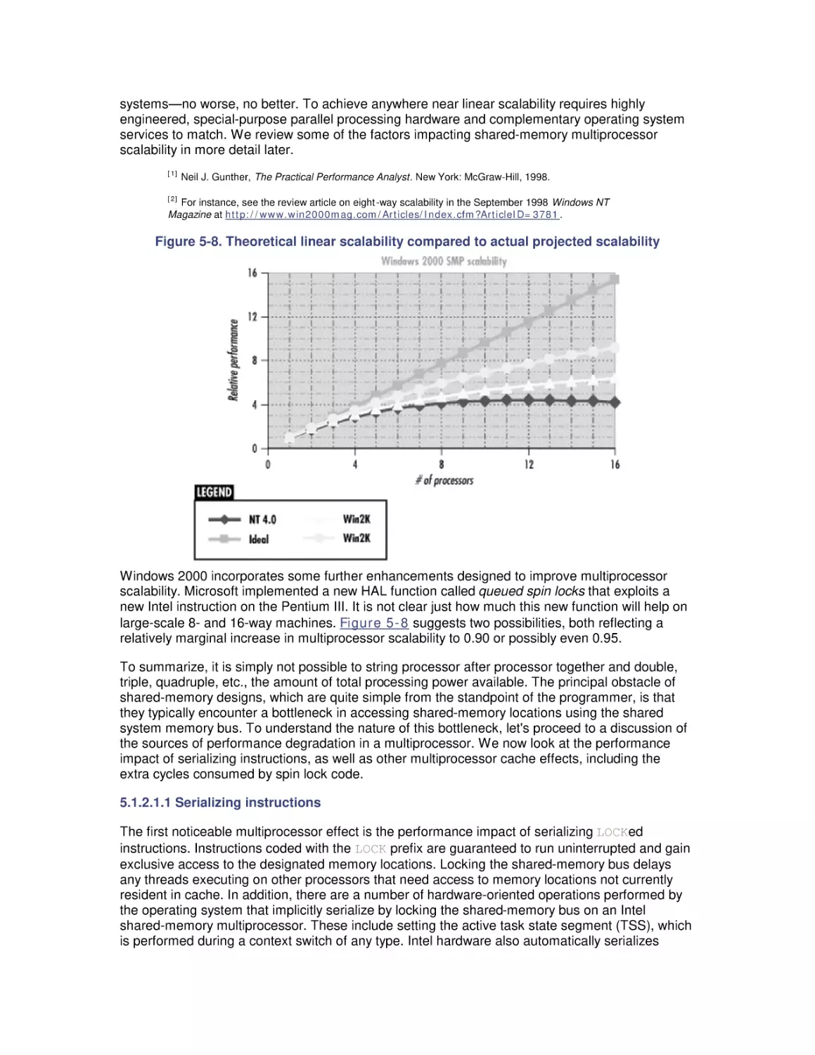
Windows 2000 Performance Guide
Odysseas Pentakalos
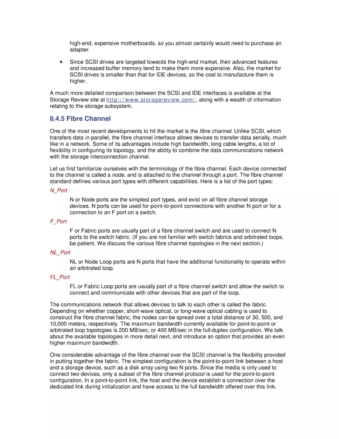
Mark Friedman
Publisher: O'Reilly
First Edition January 2002
ISBN: 1-56592-466-5, 718 pages
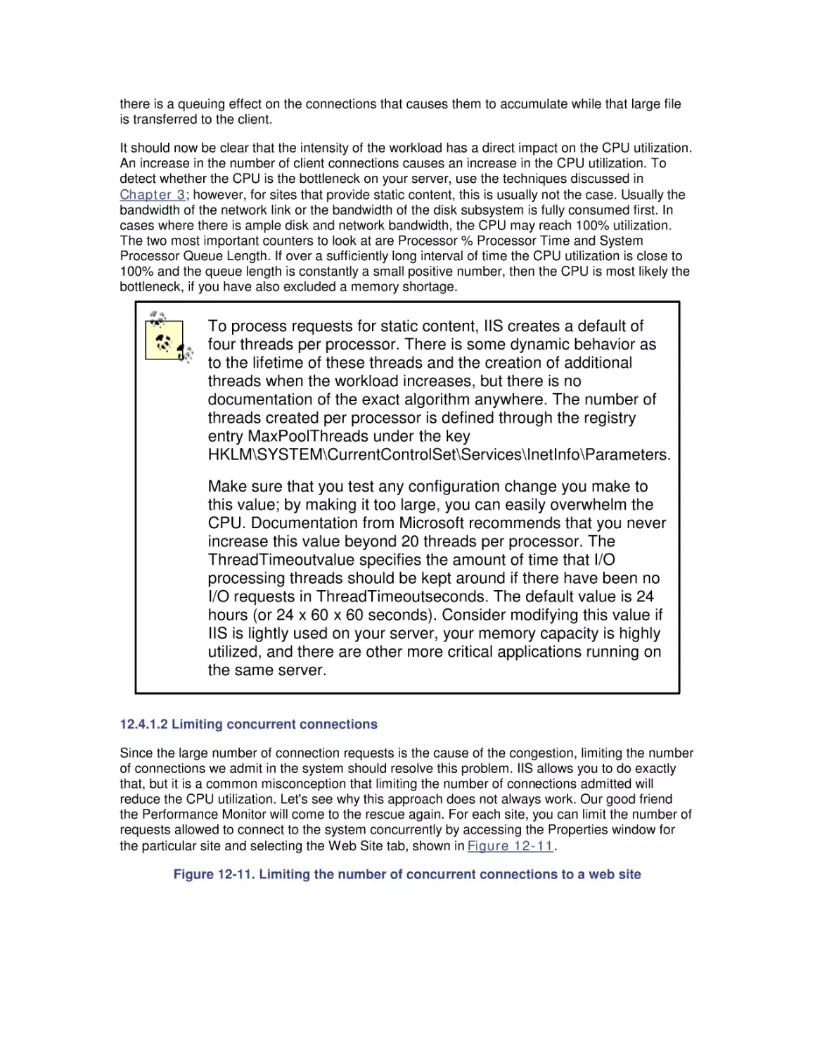
By Giantdino
Copyright
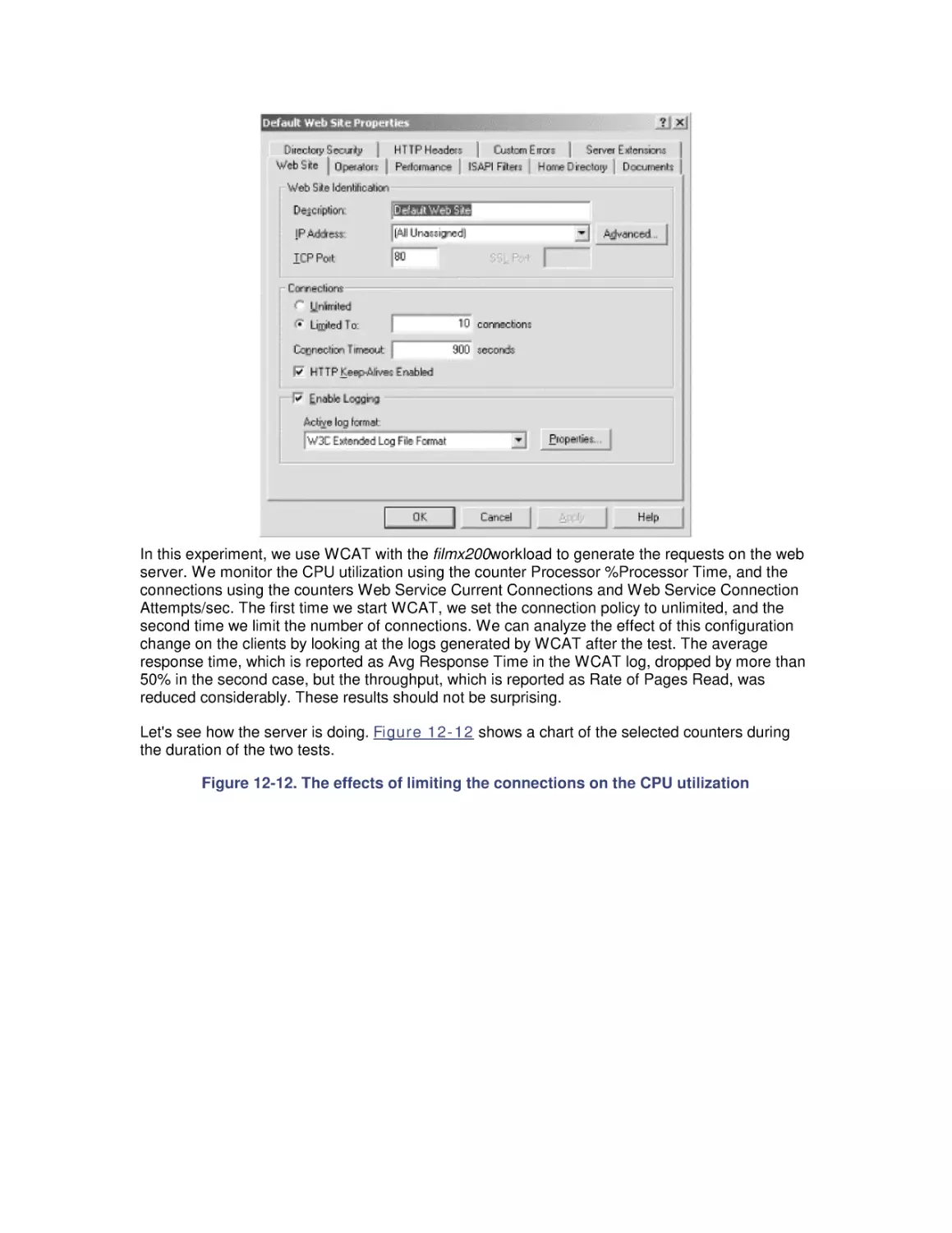
Table of Contents
Index
Full Description
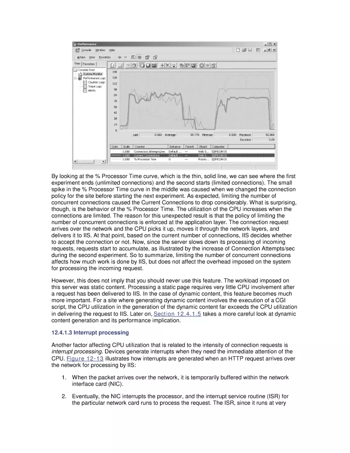
About the Author
Reviews
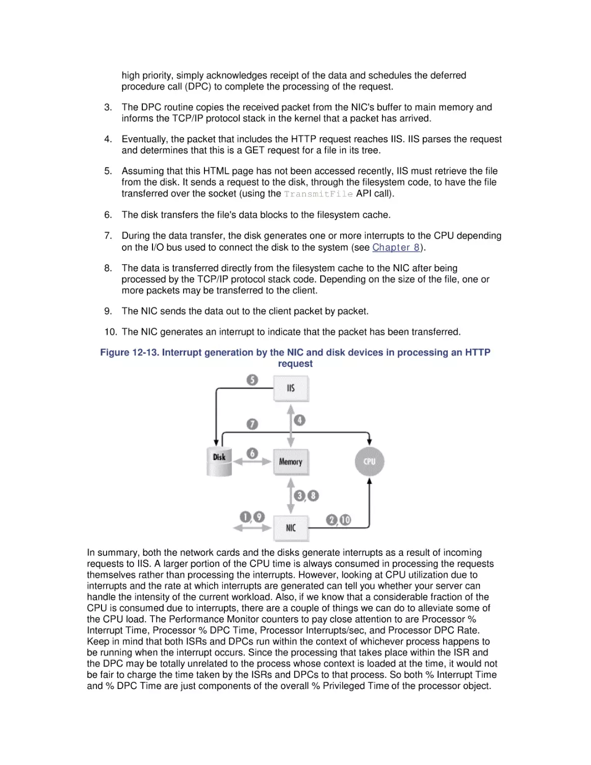
Reader reviews
Errata
Most computer systems do not degrade gradually. The painful reality
is that performance is acceptable day after day, until quite suddenly
it all falls apart. If this happnes on a system you're responsible for,
you'll need to be prepared to get your organization through the
crisis. Windows 2000 Performance Guide will give you the
information and the conceptual framework to become your own
Windows 2000 performance expert.
Windows 2000 Performance Guide
Preface
Intended Audience
Organization of This Book
Conventions Used in This Book
How to Contact Us
Acknowledgments
1. Perspectives on Performance Management
1.1 Windows 2000 Evolution
1.2 Tools of the Trade
1.3 Performance and Productivity
1.4 Performance Management
1.5 Problems of Scale
1.6 Performance Tools
2. Measurement Methodology
2.1 Performance Monitoring on Windows
2.2 Performance Monitoring API
2.3 Performance Data Logging
2.4 Performance Monitoring Overhead
2.5 A Performance Monitoring Starter Set
3. Processor Performance
3.1 Windows 2000 Design Goals
3.2 The Thread Execution Scheduler
3.3 Thread Scheduling Tuning
4. Optimizing Application Performance
4.1 Background
4.2 The Application Tuning Case Study
4.3 Intel Processor Hardware Performance
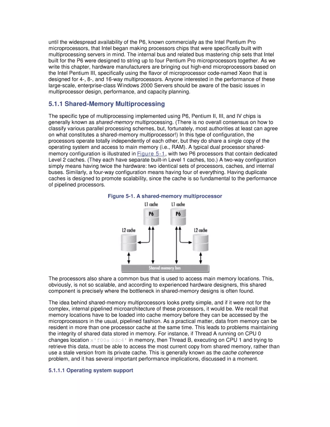
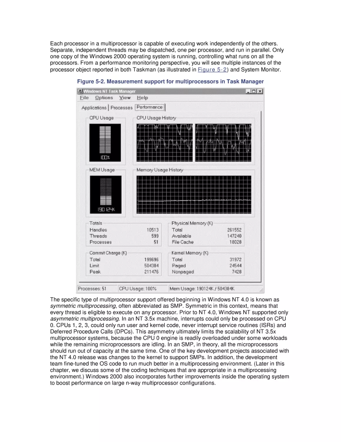
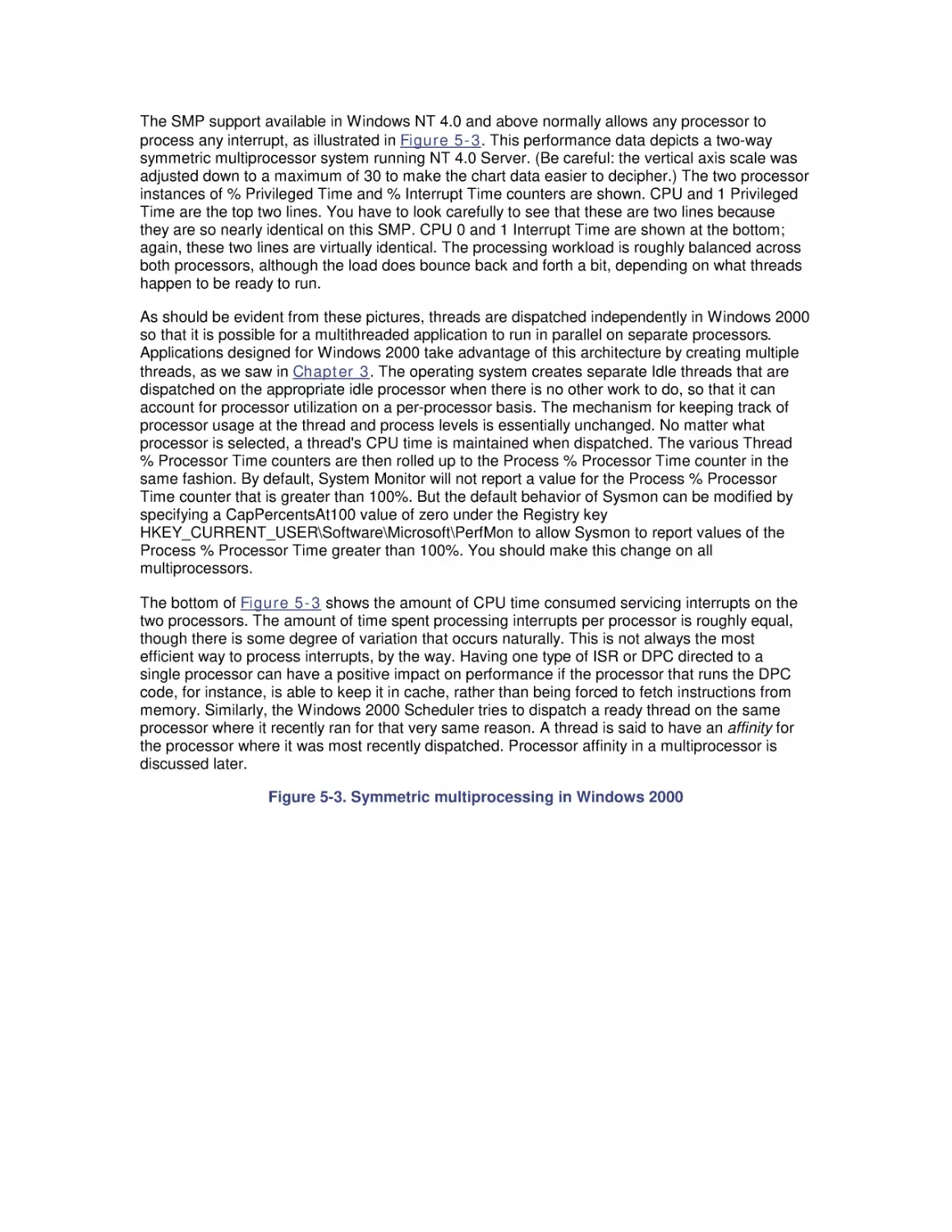
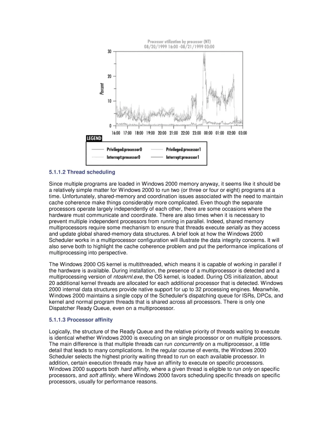
5. Multiprocessing
5.1 Multiprocessing Basics
5.2 Cache Coherence
5.3 Pentium Pro Hardware Counters
5.4 Optimization and SMP Configuration Tuning
5.5 Configuring Server Applications for Multiprocessing
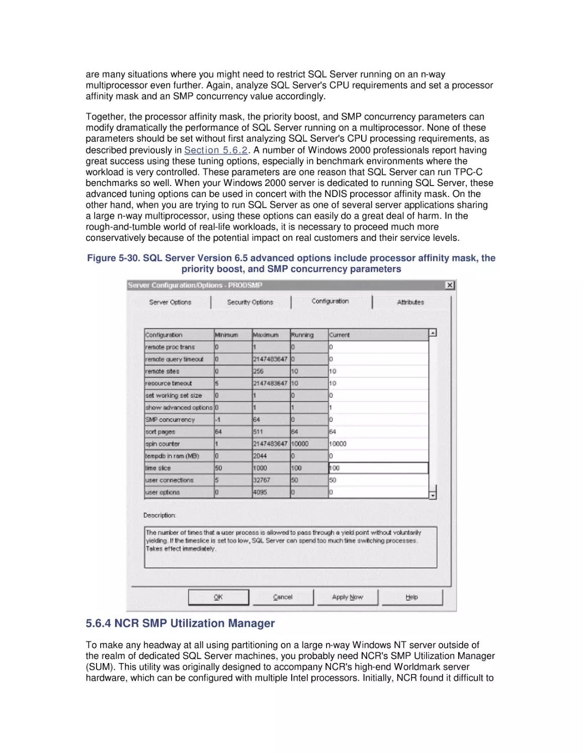
5.6 Partitioning Multiprocessors
6. Memory Management and Paging
6.1 Virtual Memory
6.2 Page Replacement
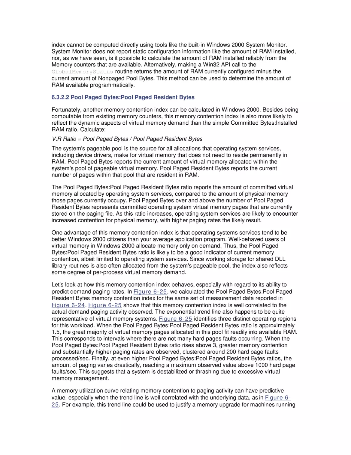
6.3 Memory Capacity Planning
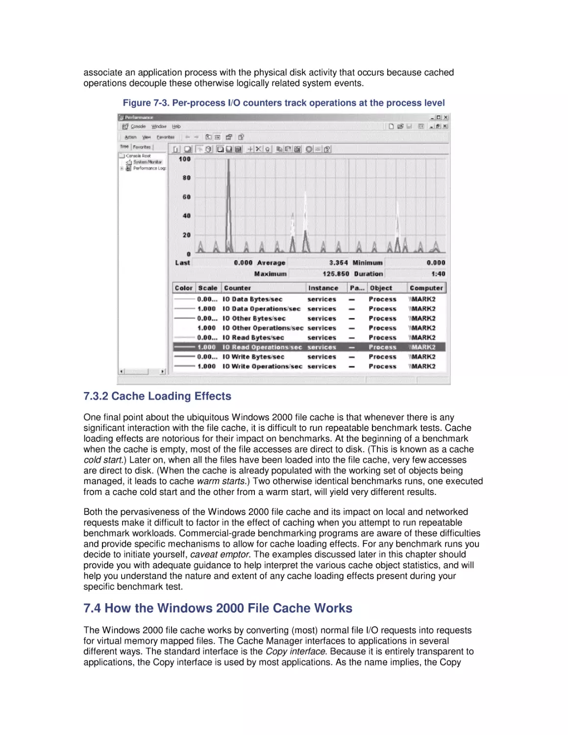
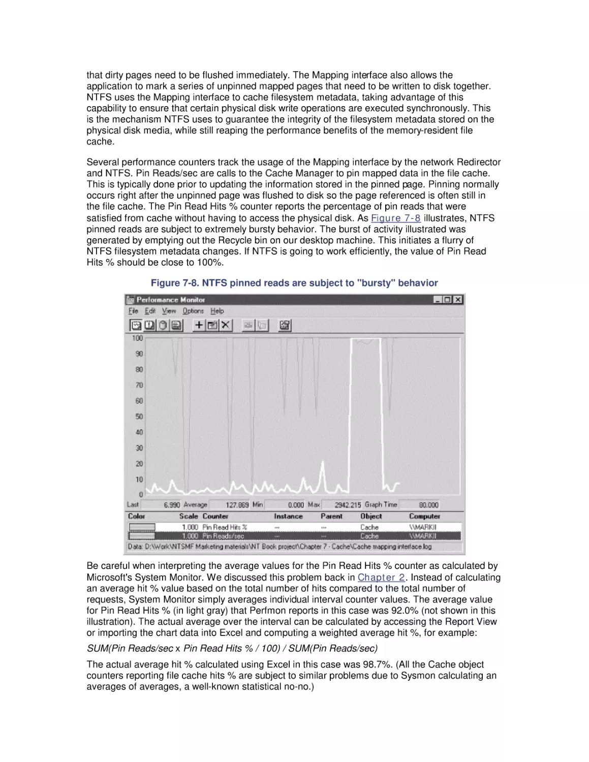
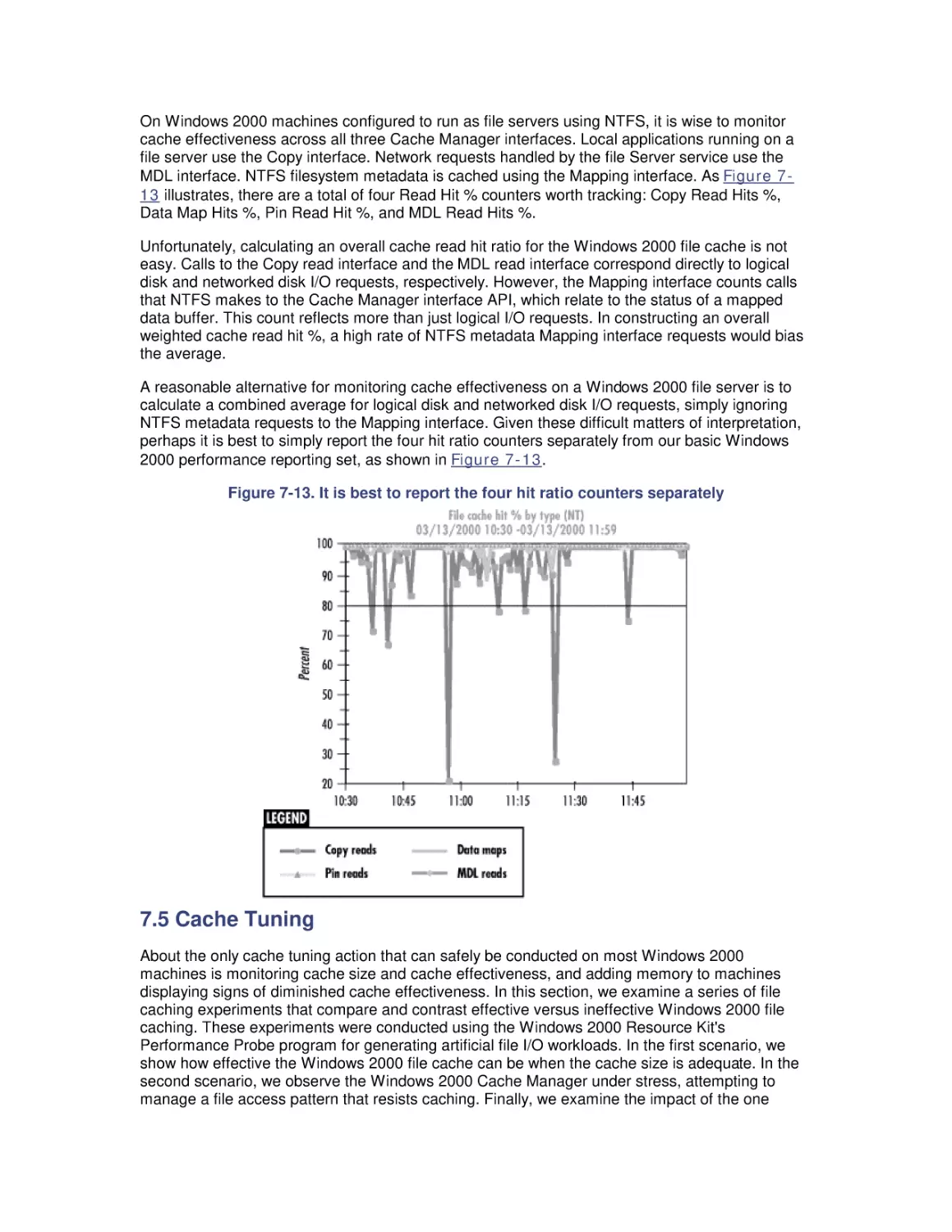
7. File Cache Performance and Tuning
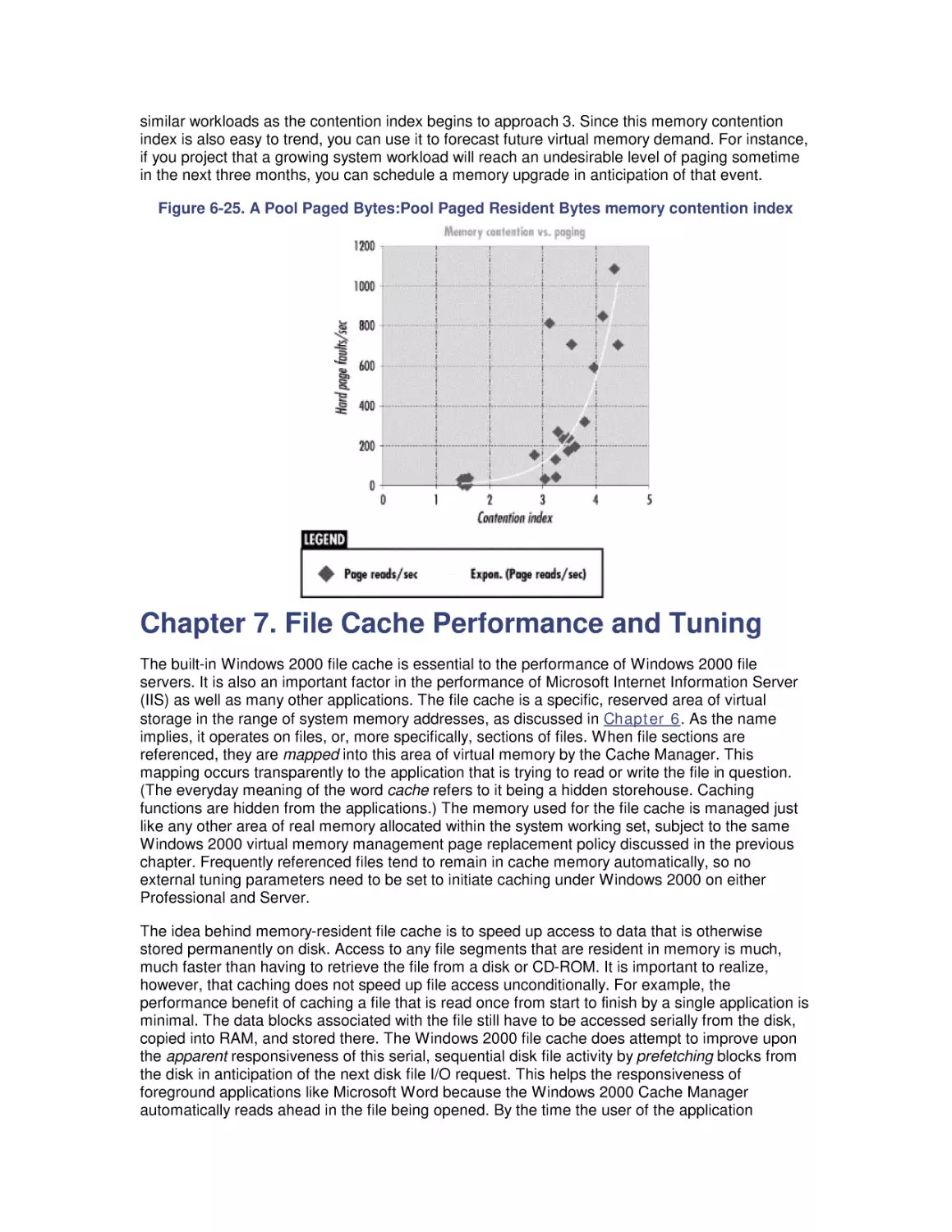
7.1 File Cache Sizing
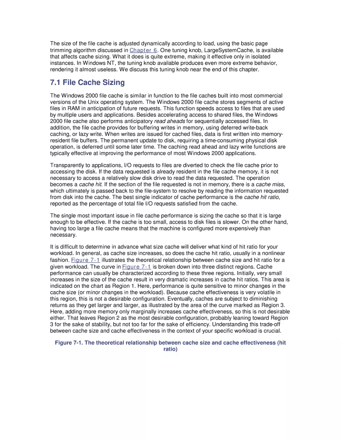
7.2 Cache Performance Counters
7.3 Universal Caching
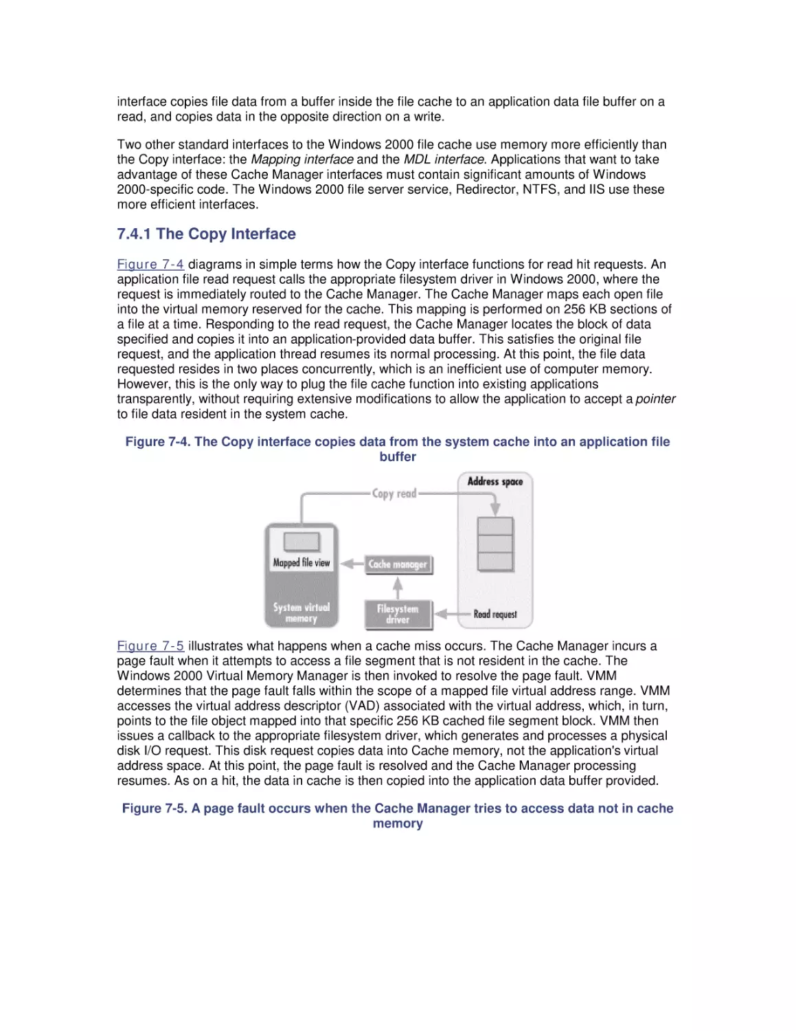
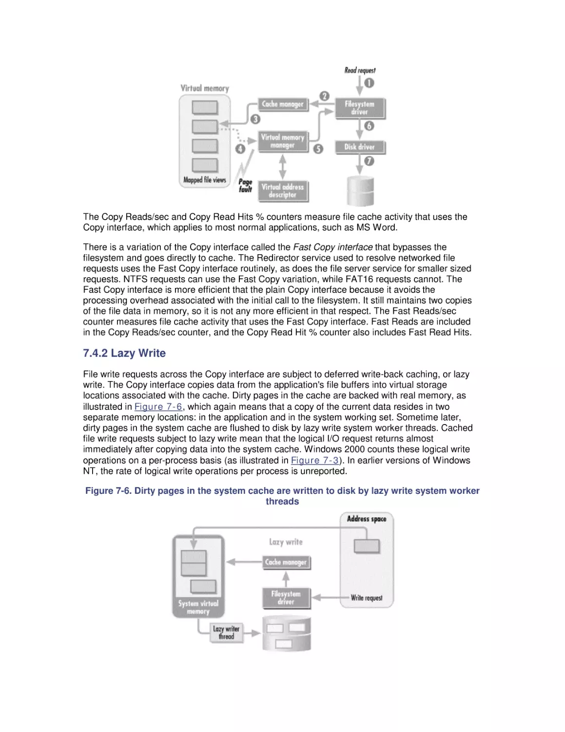
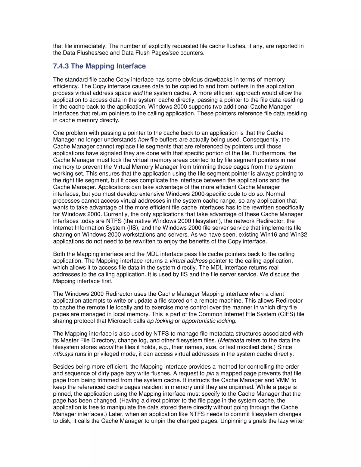
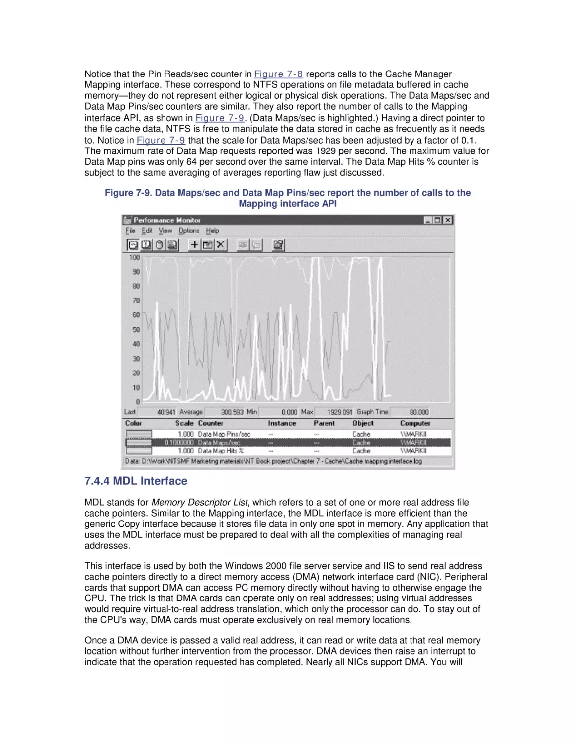
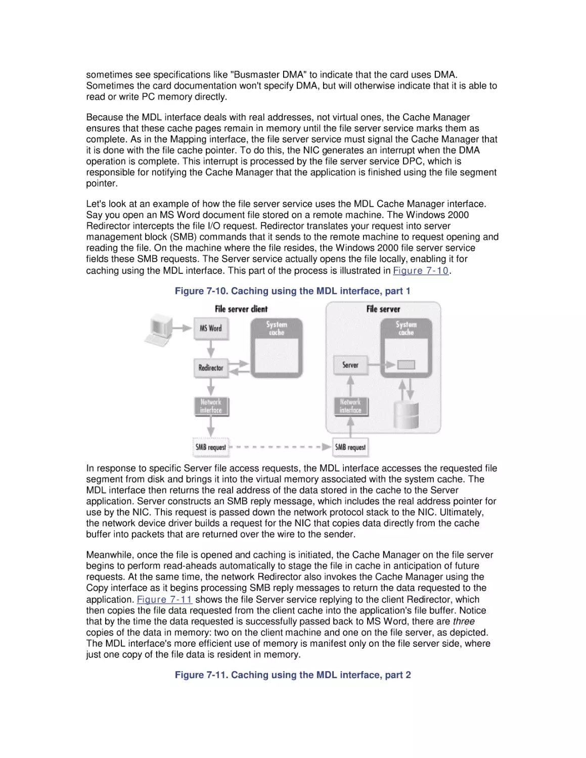
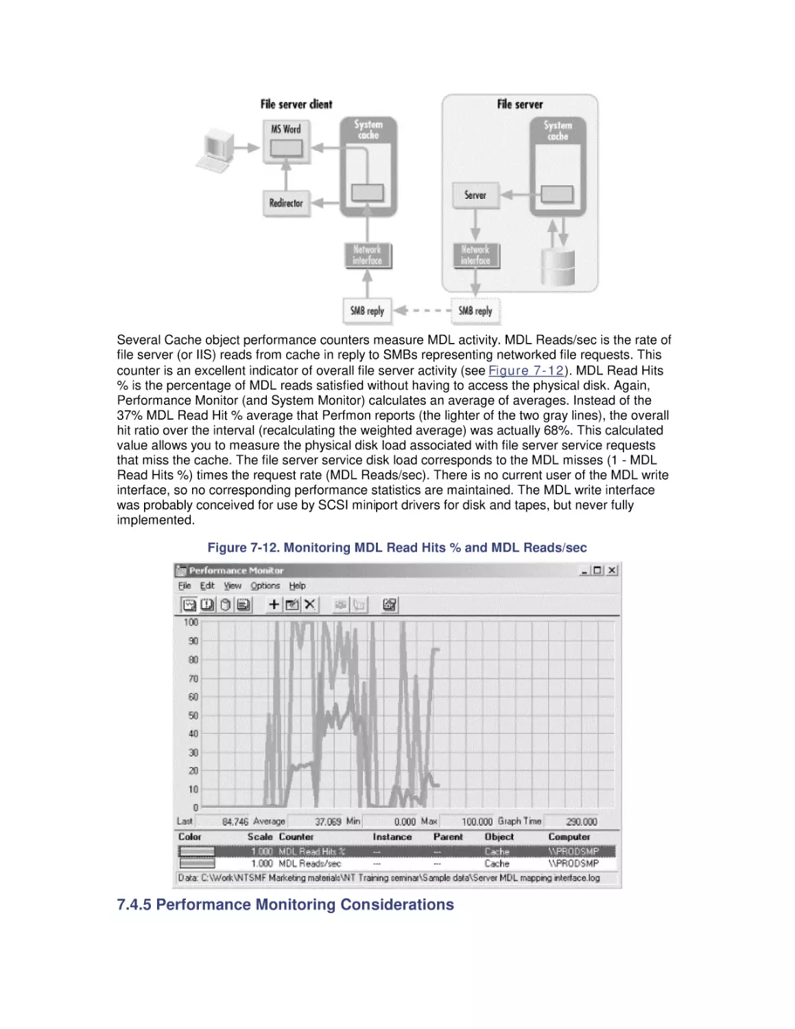
7.4 How the Windows 2000 File Cache Works
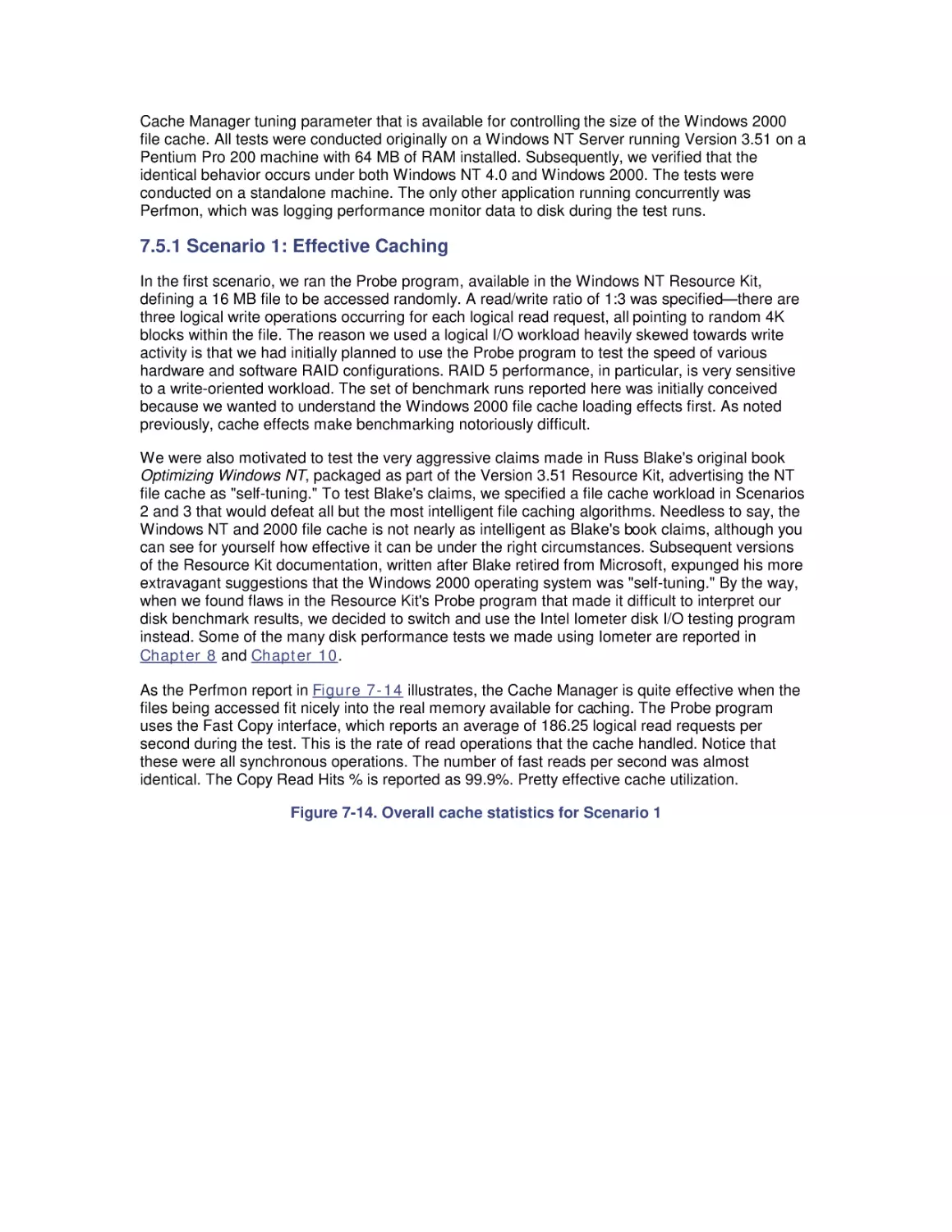
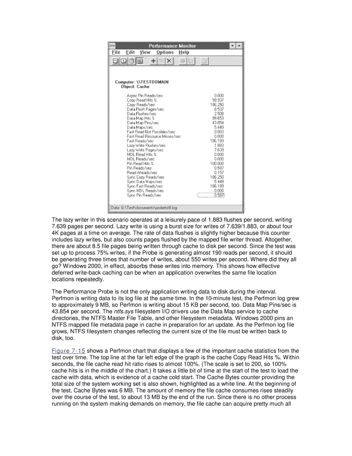
7.5 Cache Tuning
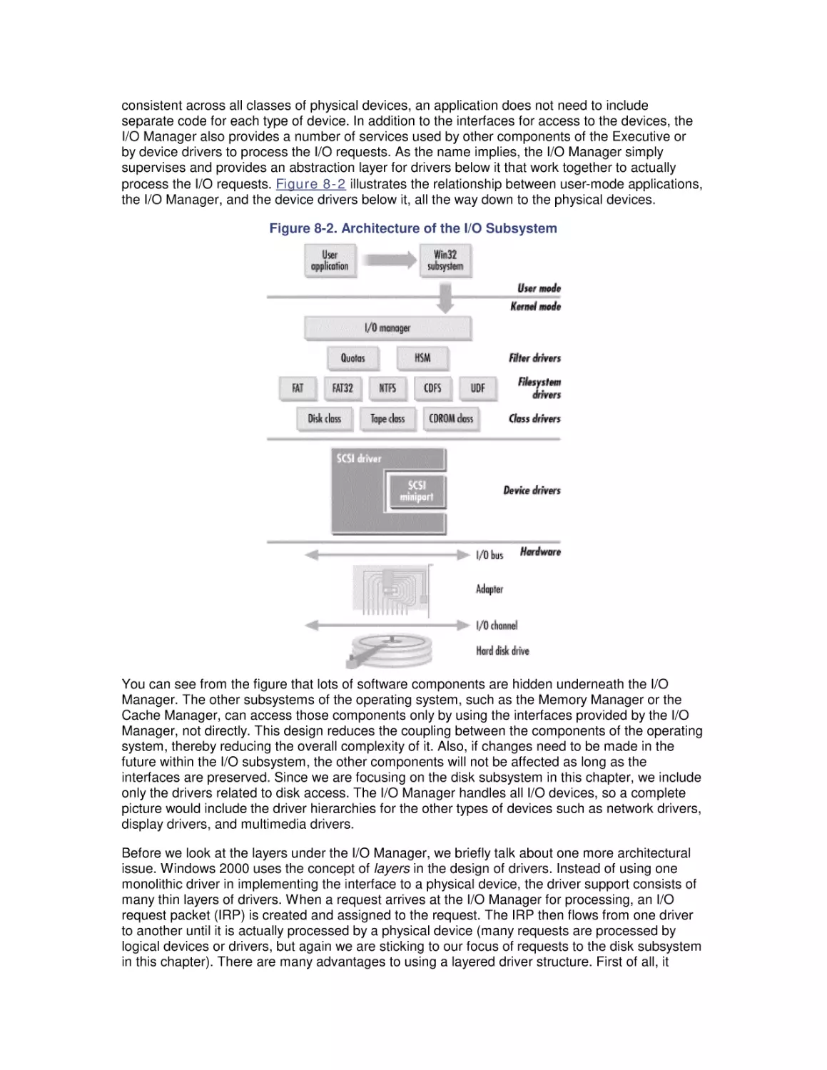
8. Disk Subsystem Performance
8.1 The I/O Subsystem
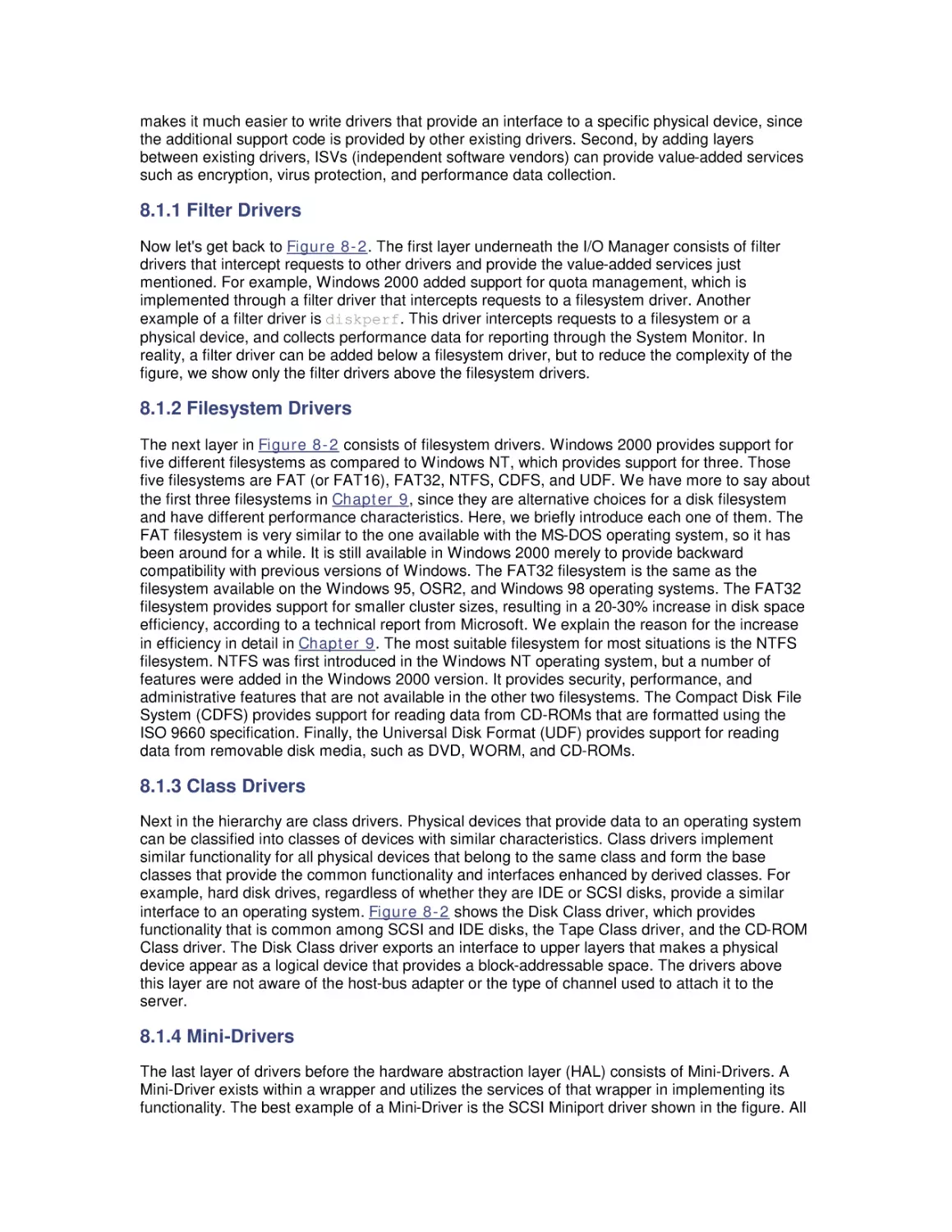
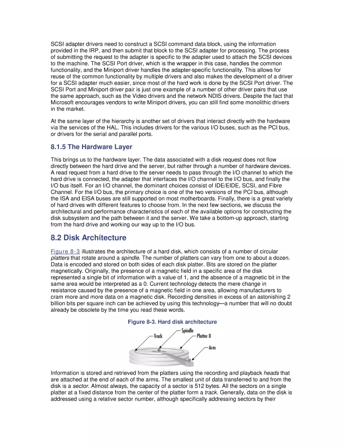
8.2 Disk Architecture
8.3 I/O Buses
8.4 Disk Interfaces
8.5 System Monitor Counters
8.6 Workload Studies
9. Filesystem Performance
9.1 Storage Management
9.2 Filesystems
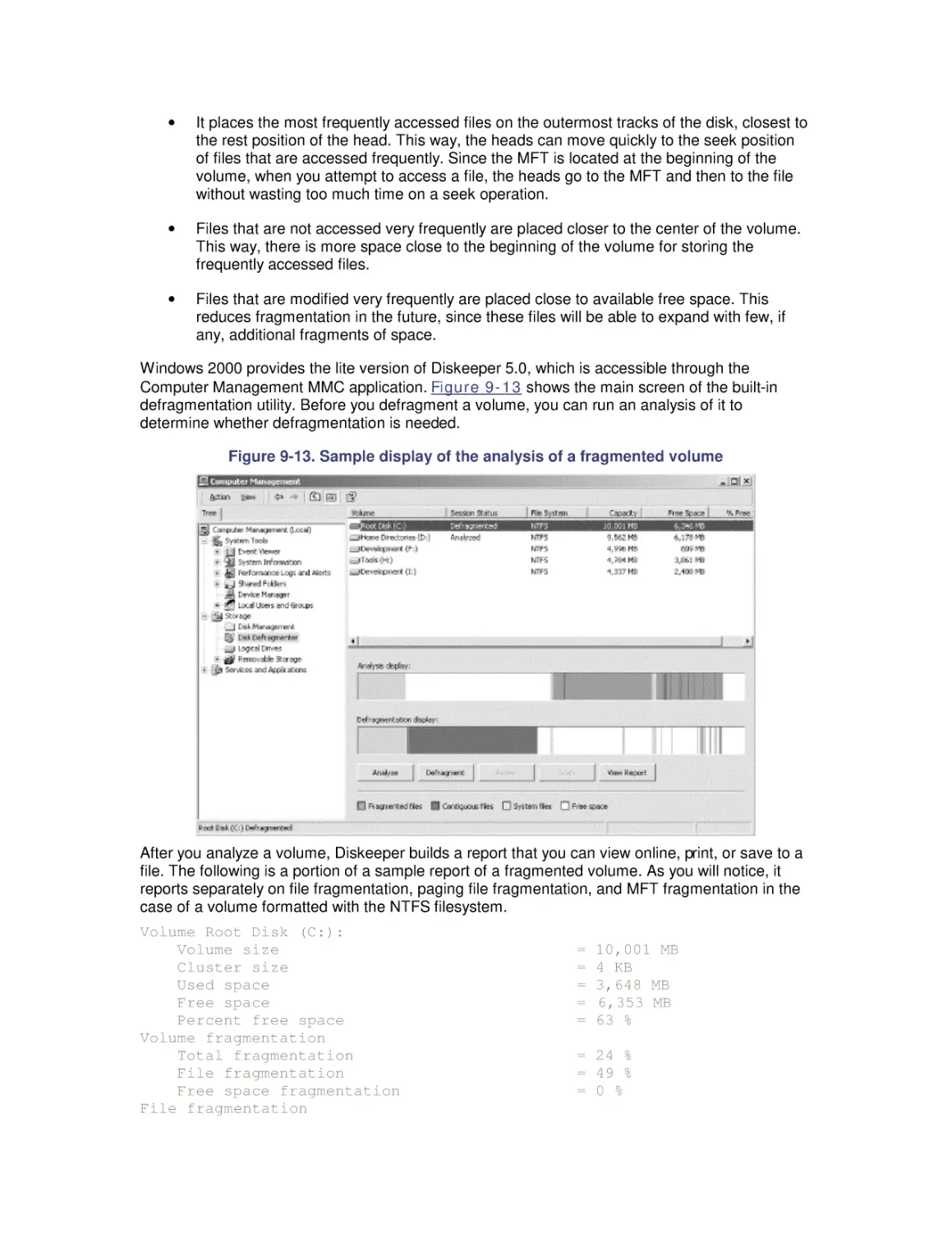
9.3 Defragmentation
9.4 System Monitor Counters
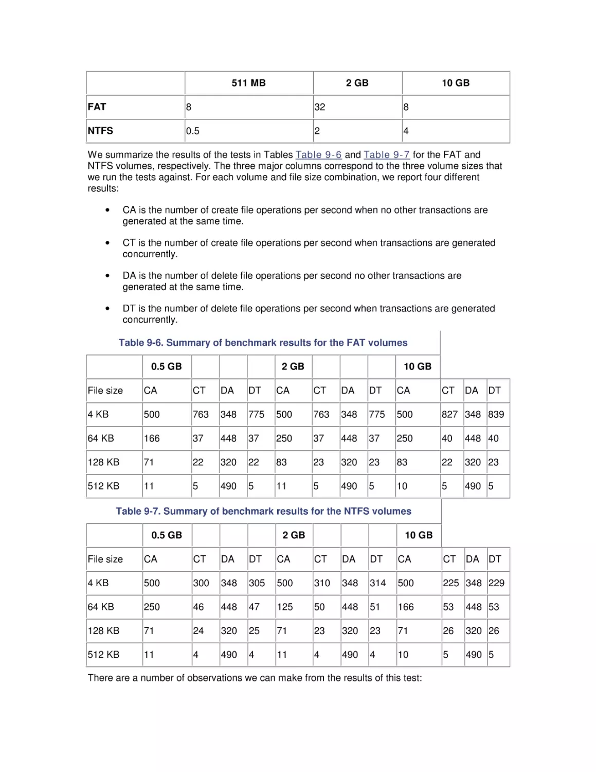
9.5 Comparing Filesystem Performance
9.6 Selecting a Filesystem
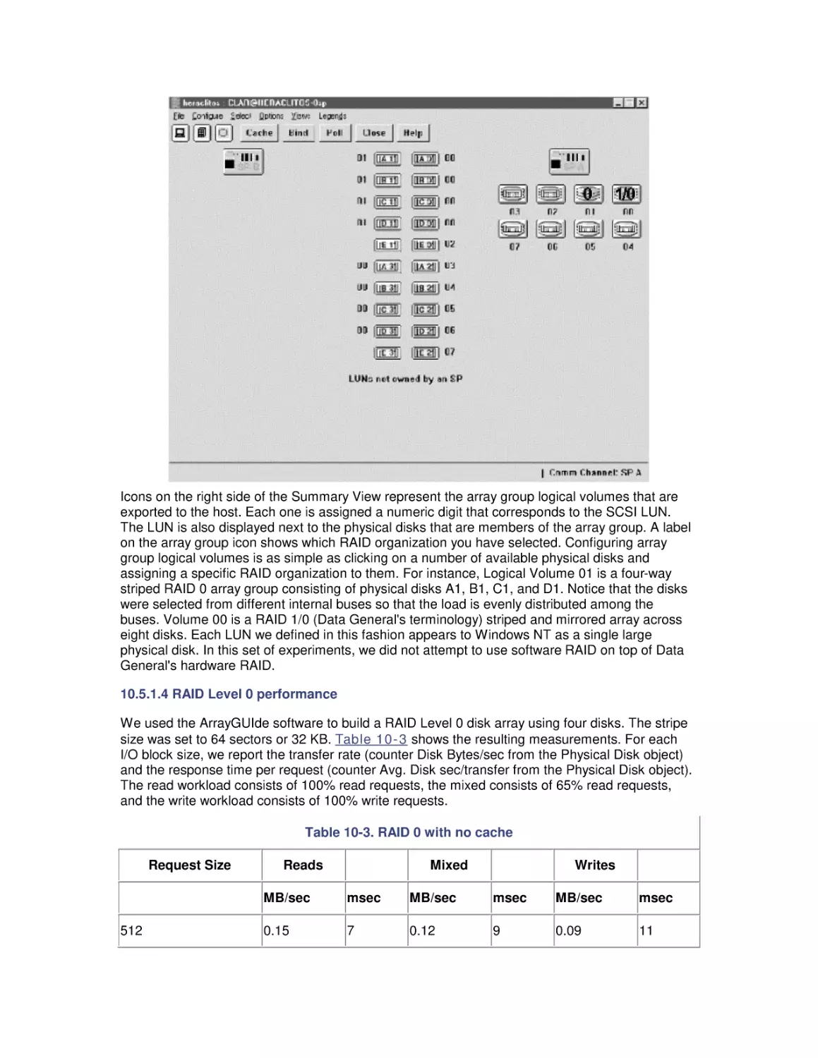
10. Disk Array Performance
10.1 Disk Striping
10.2 Enter RAID
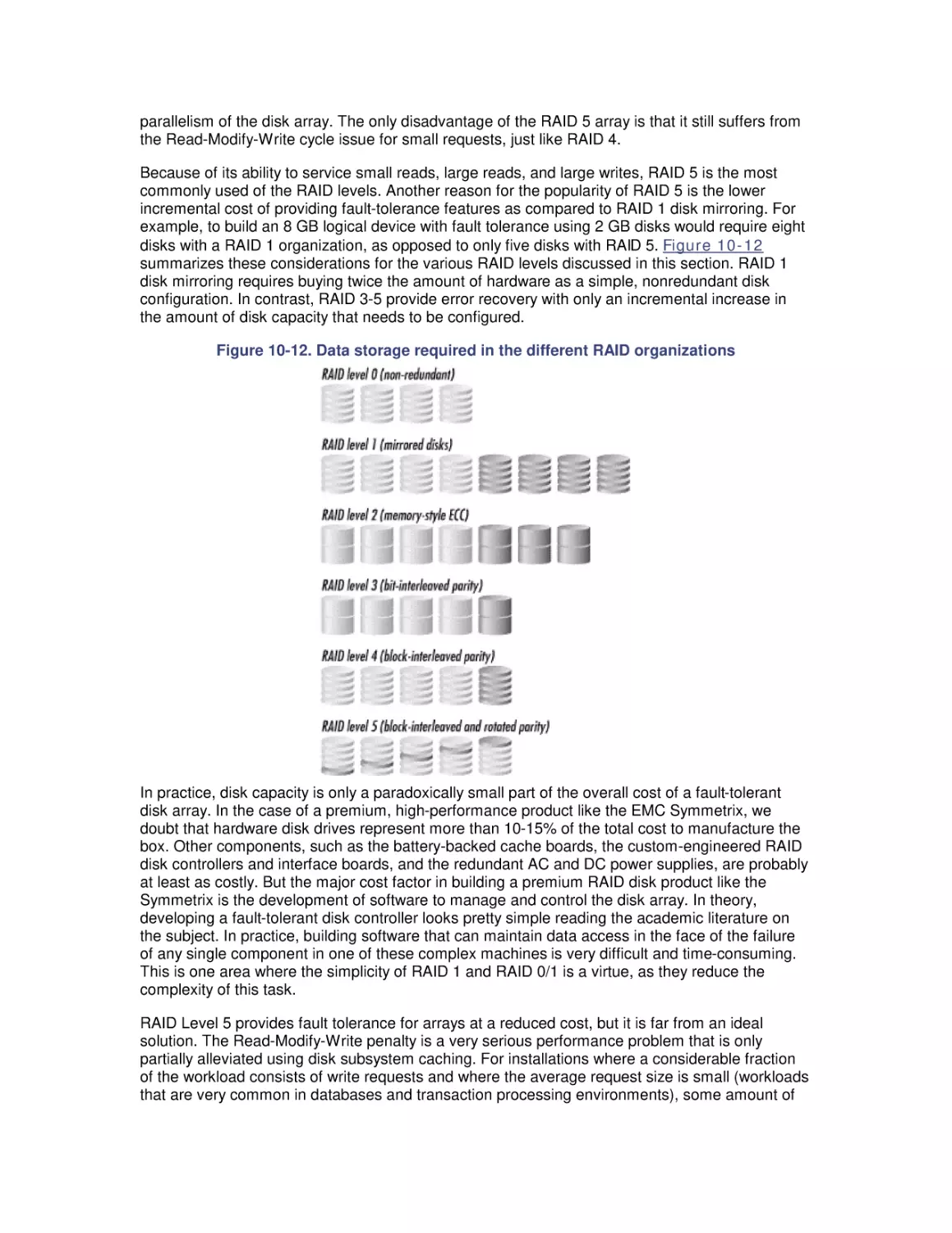
10.3 RAID Disk Organizations
10.4 RAID and Windows 2000
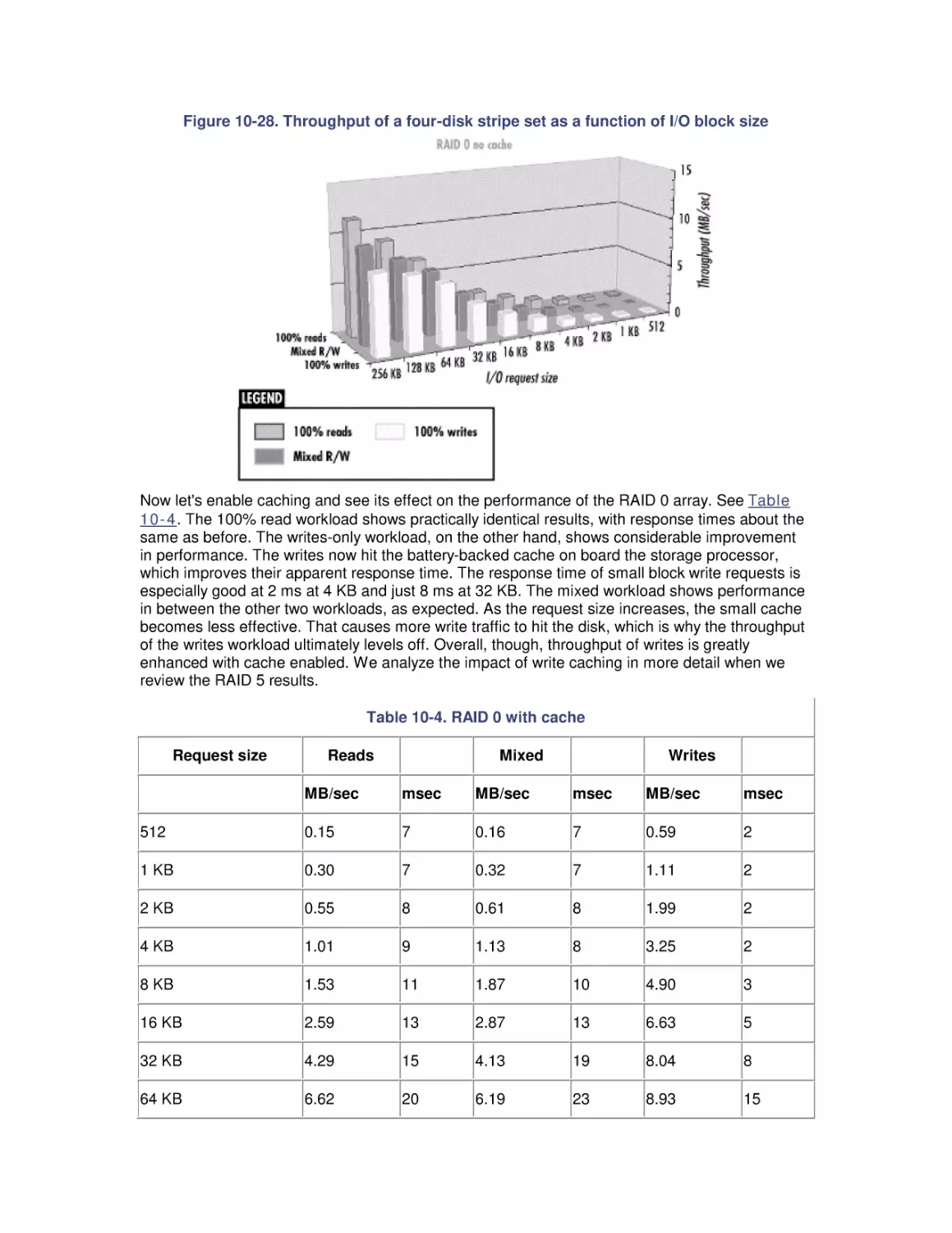
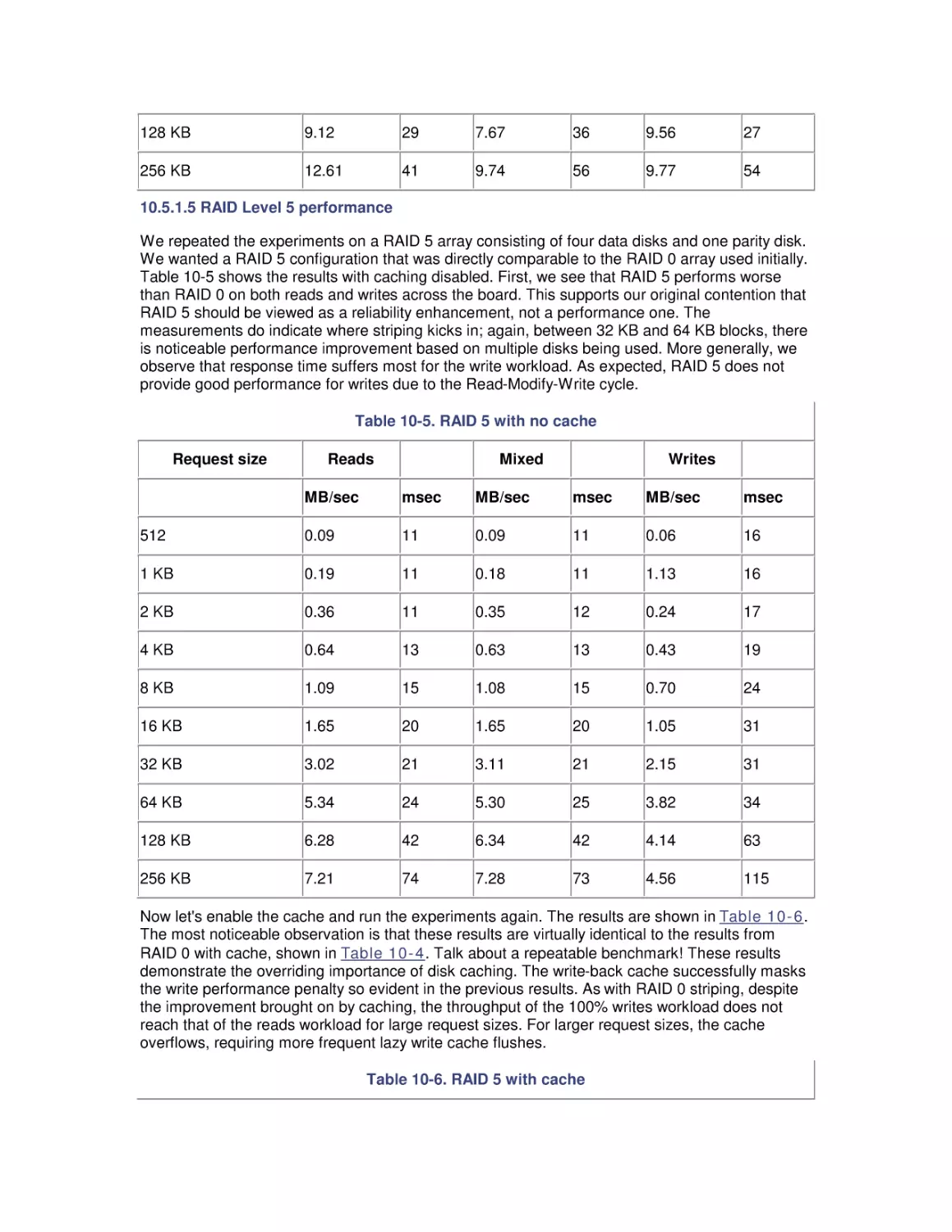
10.5 Benchmark Testing
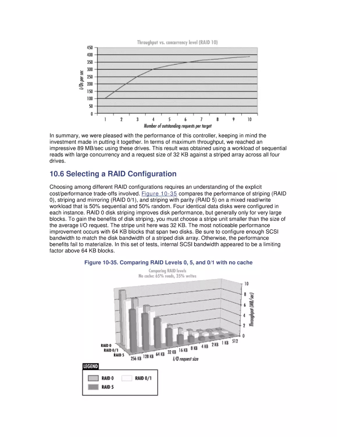
10.6 Selecting a RAID Configuration
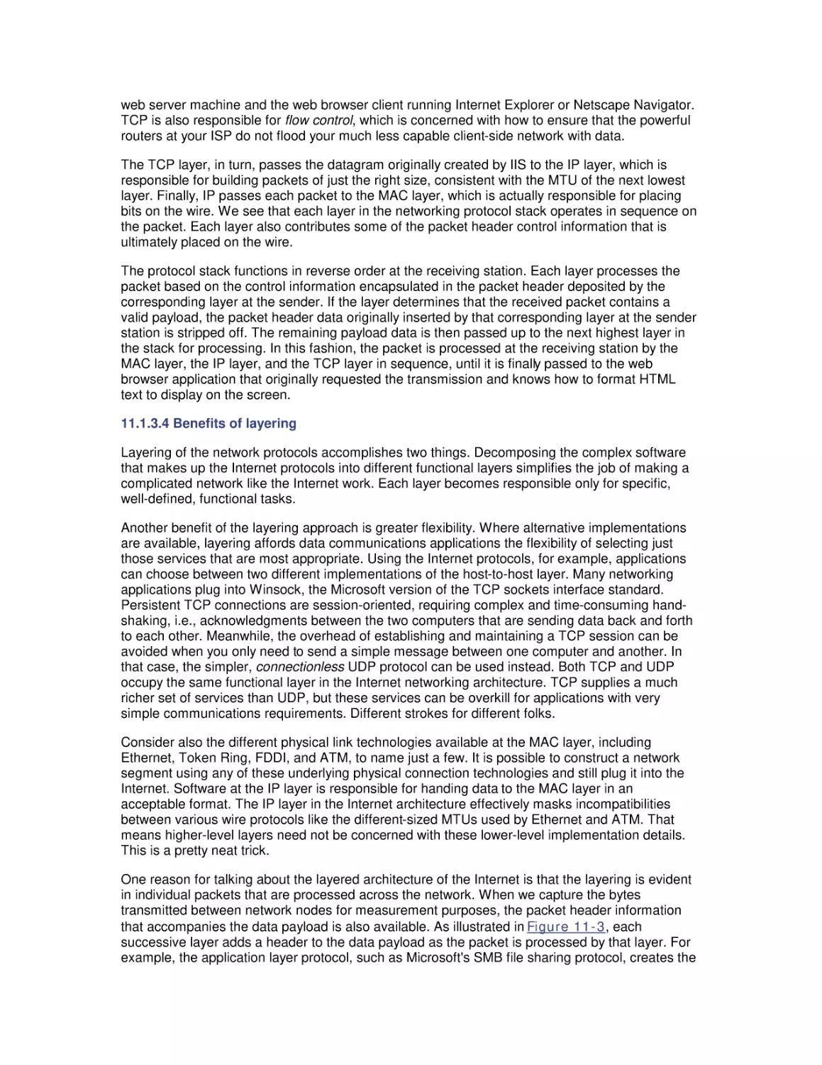
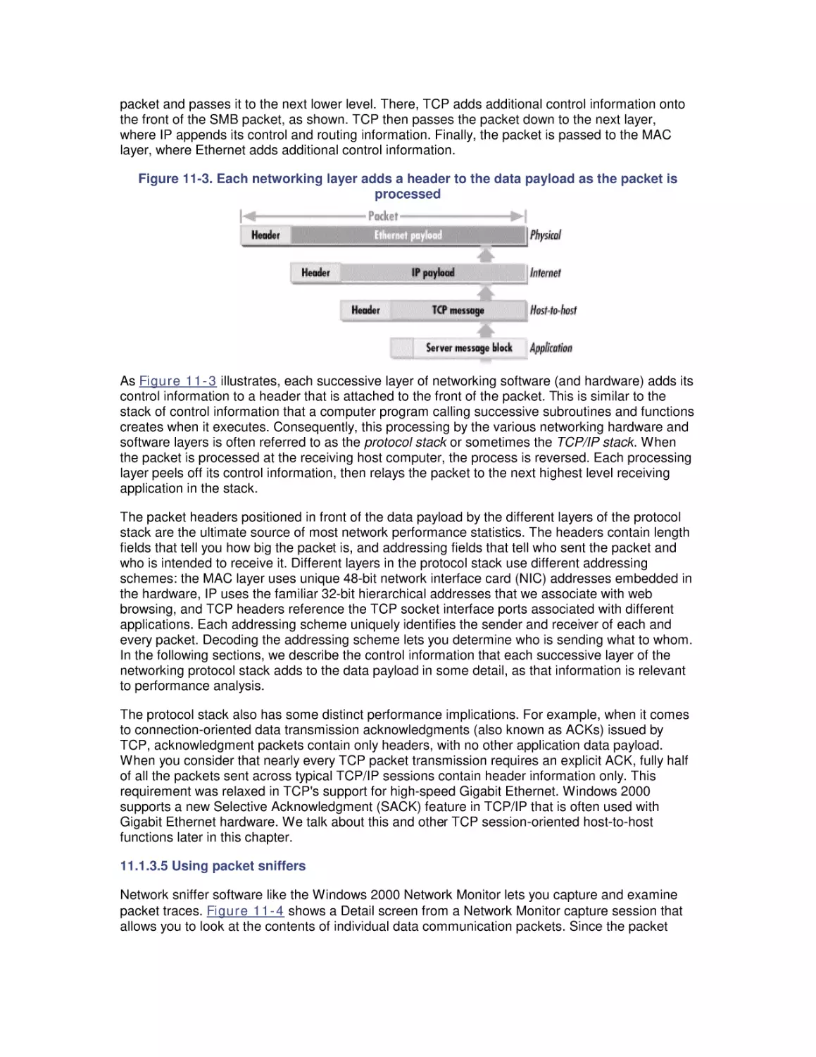
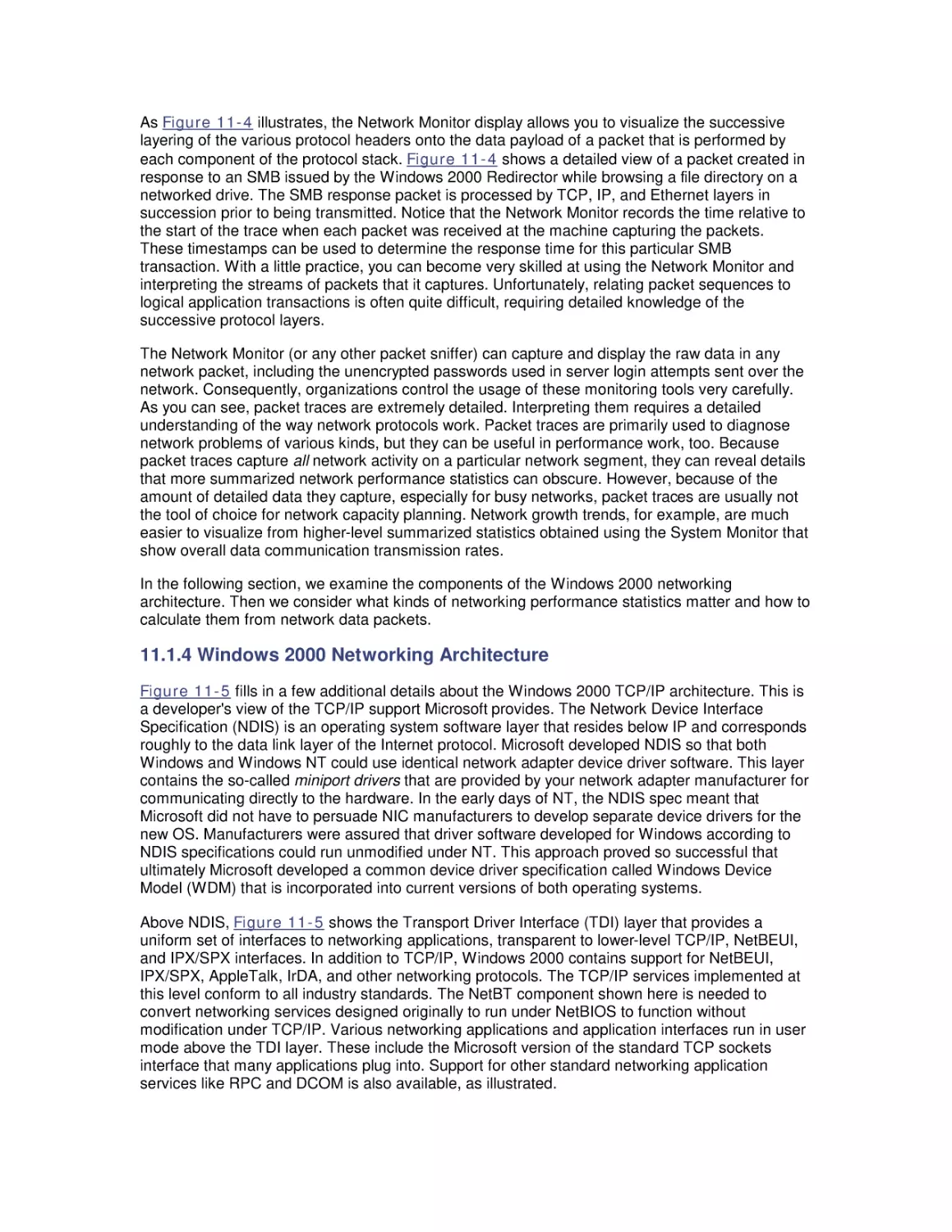
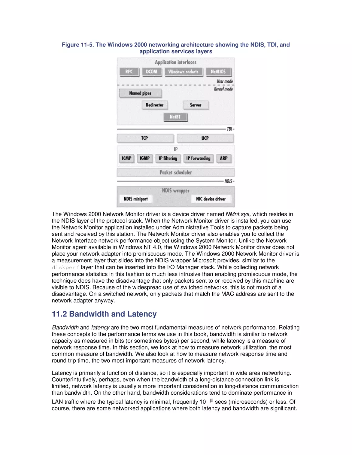
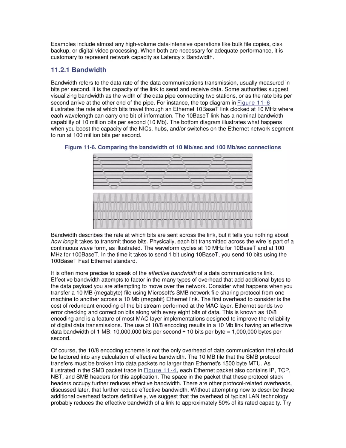
11. Introduction to Networking Technology
11.1 Networking Basics
11.2 Bandwidth and Latency
11.3 Media Access Layer
11.4 Internet Protocol Layer
11.5 Host-to-Host Connections
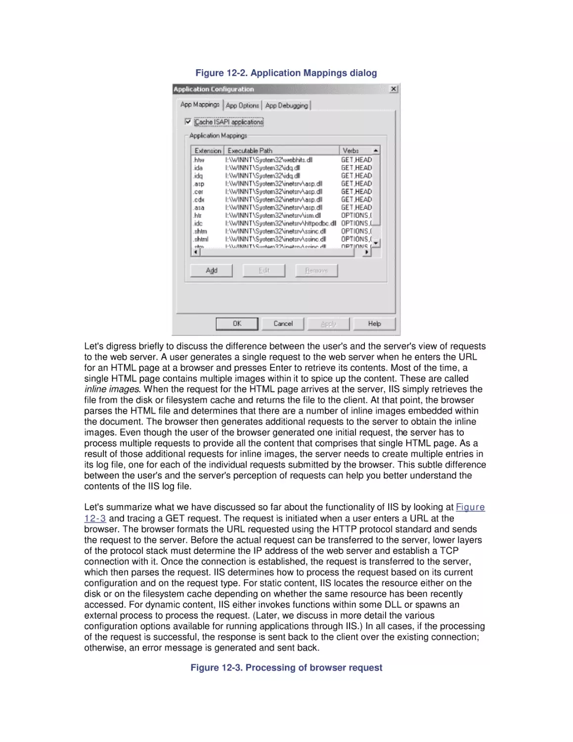
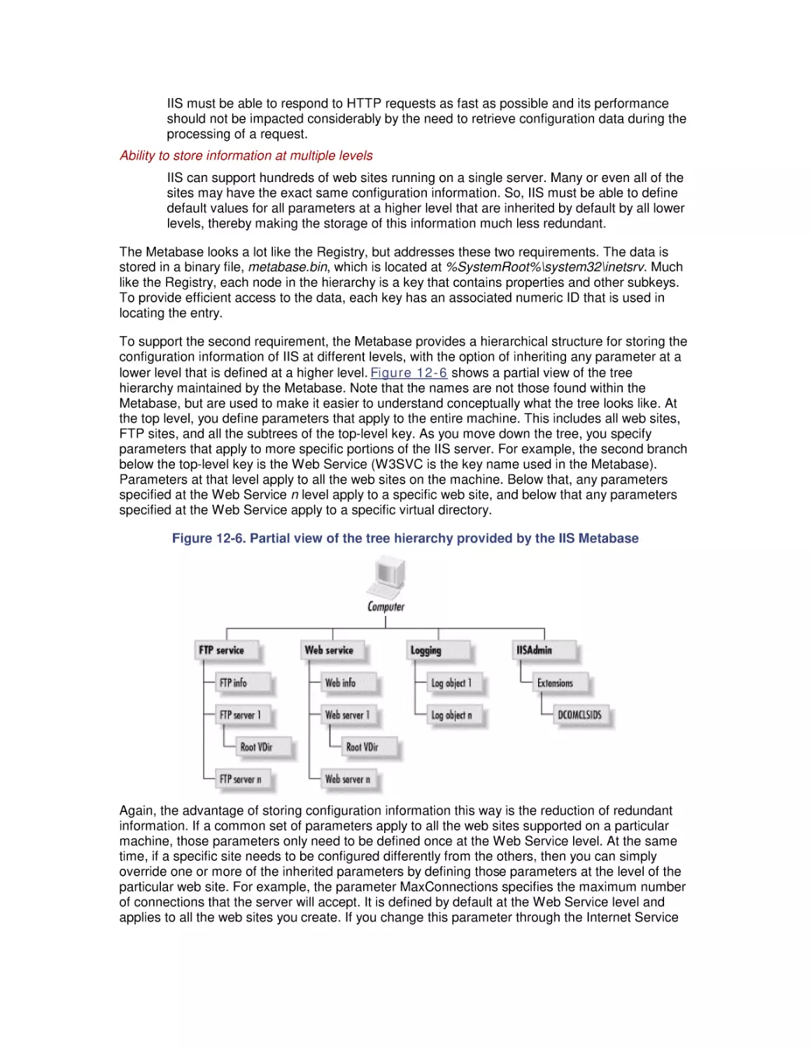
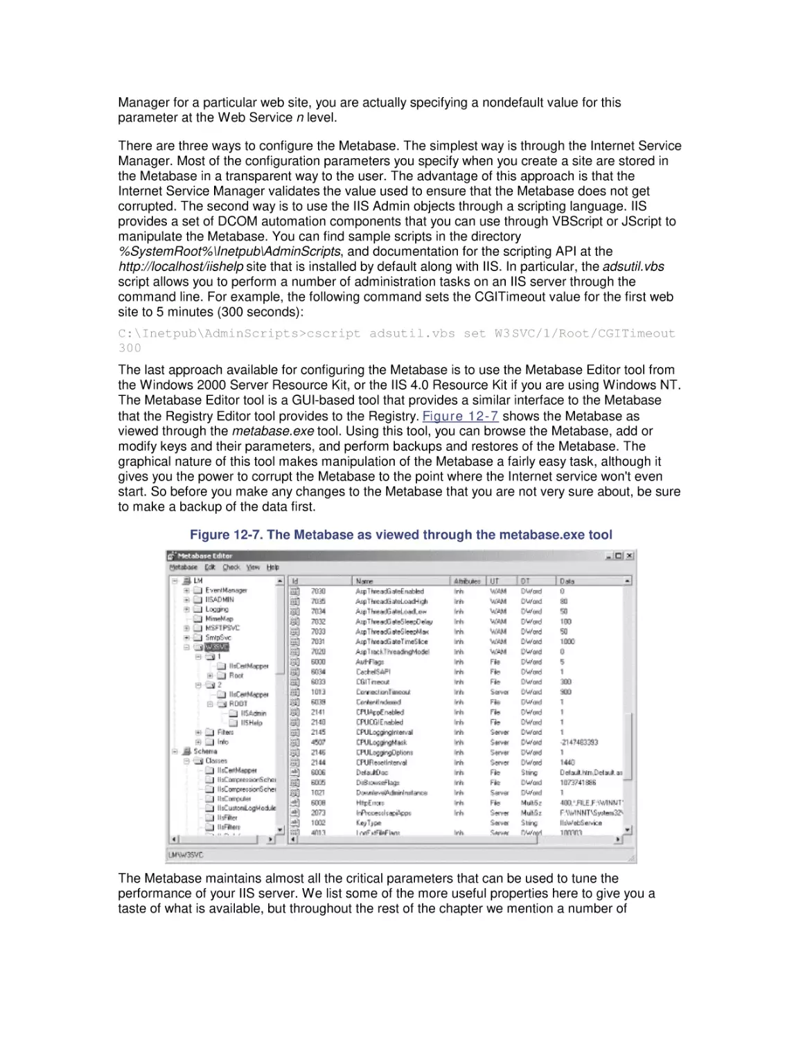
12. Internet Information Server Performance
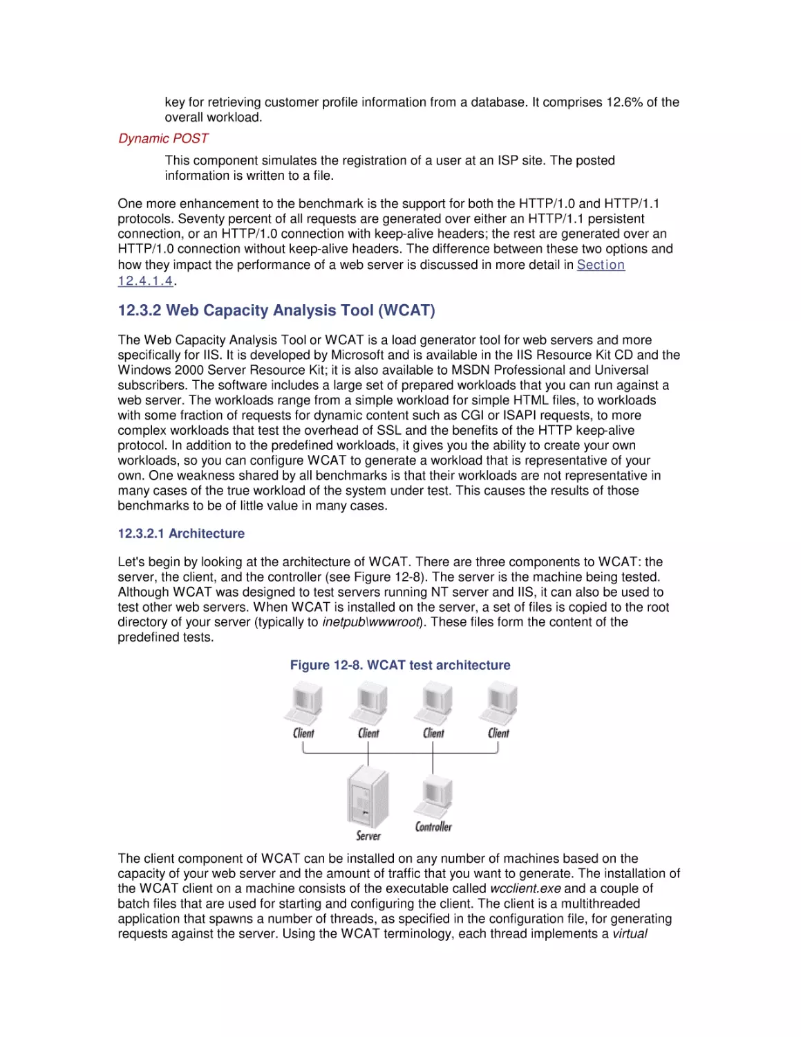
12.1 Web Server Architecture
12.2 Sources of Information
12.3 Web Server Benchmarks
12.4 Performance Management
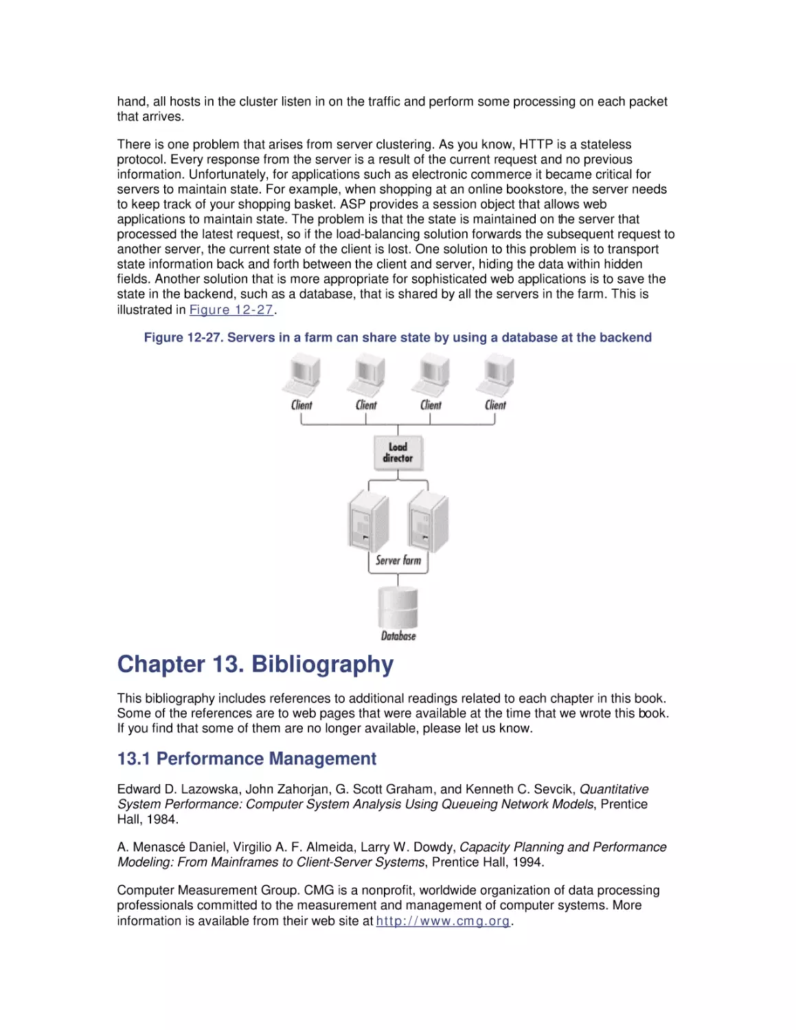
12.5 Load Balancing and Server Clustering
13. Bibliography
13.1 Performance Management
13.2 Measurement Methodology
13.3 Processor Performance
13.4 Optimizing Application Performance
13.5 Multiprocessing
13.6 Memory Management and Paging
13.7 File Cache Performance and Tuning
13.8 Disk Subsystem Performance
13.9 Filesystem Performance
13.10 Disk Array Performance
13.11 Networking Technology
13.12 Internet Information Server Performance
Colophon
Preface
The book you hold in your hands originally arose from need. Professionally, we felt the need to
answer both basic and not-so-basic questions about the performance of Intel-based computer
systems running various versions of the Microsoft Windows 2000 operating system, including
both Windows NT and Windows XP. We expect that most readers of this book are seeking
answers to common questions about computer and operating system performance out of similar
personal or professional curiosity. This book, in fact, evolved from a seminar intended to address
such questions that one of the authors developed and taught over a number of years.
The material in the book is the result of research performed over the last five years on successive
versions of the Windows NT operating system, beginning with Version 3.5 and continuing to the
present day. (As this book was going to press, we were experimenting with early versions of
Windows XP. As best we can currently determine, almost all of the information provided here
regarding Windows 2000 performance can also be applied to the 32-bit version of Windows XP.)
Much of the material here is original, derived from our observations and analysis of running
systems, some of which may contradict official documentation and the writings and
recommendations of other authorities. Rest assured that we carefully reviewed any findings
reported here that run counter to the received wisdom.
While we strive to make the discussion here definitive, there are necessarily many places where
our conclusions are tentative and subject to modification should new information arise. We expect
readers to be willing to challenge our conclusions in the face of strong empirical evidence to the
contrary, and urge you to communicate to us (via the publisher) when you discover errors of
commission or omission, for which we assume full responsibility. If you observe behavior on one
of your Windows 2000 machines that seems to contradict what we say in the book, please share
those observations with us. With your help, we should be able to produce a subsequent version
of this book that is even more authoritative.
Our research for the book began with all the standard sources of information about the Windows
2000 operating system. We frequently cite official documentation included in the operating
system help files. We also refer to the extensive reference material provided in the Windows 2000
Resource Kit. David Solomon and Mark Russinovich's Inside Windows 2000, published by
Microsoft Press, was another valuable source of inside information. The Windows 2000 platform
System Development Kit (SDK) and Device Driver Development Kit (DDK) documentation, along
with Microsoft Developer Network (MSDN) KnowledgeBase entries and other technical articles,
also proved useful from time to time. Intel processor hardware documentation (available at
http://www.intel.com) was helpful as well, particularly in writing Chapter 4 and Chapter 5.
At many points in the text, we cite other reference material, including various academic journals
and several excellent books. From time to time, we also mention worthy magazine articles and
informative white papers published by various vendors. This book contains a complete
bibliography.
Originally, we intended this book to serve as an advanced text, picking up where Russ Blake's
outstanding Optimizing Windows NT left off. Unfortunately, Blake's book is currently out of print
and woefully obsolete. Blake led a team of developers who implemented a performance
monitoring API for the initial version of Windows NT 3.1, when the OS first became available in
1992. Russ's book also documented using Performance Monitor, the all-purpose performance
monitoring application the team developed. We acknowledge a tremendous debt to Russ, Bob
Watson, and other members of that team. Writing when he did, Blake had little opportunity to
observe real-world Windows NT environments. Consequently, almost all the examples he
analyzes are based on artificial workloads generated by an application called Performance Probe,
which he also developed. (The Performance Probe program is no longer available in the
Windows 2000 Resource Kit; it is available in earlier versions of the NT 3.5 and 4.0 Resource
Kits.)
While we also experiment in places with artificial workloads running under controlled conditions,
we were fortunate to dive into Windows NT some years after it first became available. That
allowed us to observe and measure a large number of real-world Windows NT and Windows
2000 machine environments. One advantage of real-world examples and case studies is that they
are more likely to resemble the environments that you encounter. We should caution you,
however, that many of the examples we chose to write about reflect extreme circumstances
where the behavior we are trying to illustrate is quite pronounced. However, even when the
systems you are observing do not evidence similar exaggerated symptoms, you should still be
able to apply the general principles illustrated.
Our focus is on explaining how Windows 2000 and various hardware components associated with
it work, how to tell when the performance of some application running under Windows 2000 is not
optimal, and what you can do about it. The presentation is oriented toward practical problemsolving, with an emphasis on understanding and interpreting performance measurement data.
Many realistic examples of performance problems are described and discussed.
Intended Audience
We have tried to aim this book at a variety of computer systems professionals, from system
administrators who have mastered the basics of installing and maintaining Windows 2000 servers
and workstations, to developers who are trying to build high-performance applications for this
platform, to performance management and capacity planning professionals with experience on
other platforms. Although we presume no specific background or prior level of training for our
readers, our experience teaching this material suggests that this is not a book for beginners. If
you find the material at hand too challenging, we recommend reading a good book on Windows
2000 operating system internals or on basic operating system principles first. We try to pick up
the discussion precisely where most other official documentation and published sources leave off.
This includes the course material associated with obtaining MCSE certification, which provides a
very limited introduction to this topic.
Computer performance remains a core topic of interest to experienced programmers, database
administrators, network specialists, and system administrators. We wrote this book for
professionals who seek to understand this topic in the context of Windows 2000 and the
hardware environment it supports. At a minimum, you should have a working knowledge of
Windows 2000. We recommend that you have read and are familiar with the section on
performance in the Windows 2000 Professional Resource Kit, which introduces the topic and
documents the basic tools. For best results, you should have ready access to a computer running
Windows 2000 Professional or Server so that you can refer frequently to a live system while you
are reading, and put the abstract concepts we discuss into practice.
We understand that many people will buy this book because they hope it will assist them in
solving some specific Windows 2000 performance problem they are experiencing. We hope so,
too. Please understand, though, that for all but the simplest applications, there may be many
possible solutions. While we do try to provide specific and detailed answers to Frequently Asked
Questions, our approach to problem diagnosis is more theoretical and general than the many
books that promise that this sort of understanding is easily acquired. It is possible that we have
chosen to illustrate a discussion of some topic of immediate interest with an example that looks
remarkably similar to a problem that you currently face. We all get lucky from time to time.
Organization of This Book
This book consists of twelve chapters and a bibliography.
Chapter 1 introduces a broad range of best practices in computer performance and capacity
planning.
Chapter 2 describes the Windows 2000 performance monitoring API, which is the source of
most of the performance data that is dealt with in subsequent chapters.
Chapter 3 discusses the basics of processor performance monitoring at the system, processor
engine, process, and thread levels. Since the thread, not the process, is the unit of execution in
Windows 2000, we focus on thread scheduling and thread execution priority.
Chapter 4 is organized around a description of a programming optimization exercise that
compares and contrasts several popular CPU usage code-profiling tools.
Chapter 5 discusses performance considerations when you are running Windows 2000 Server,
Advanced Server, and Datacenter on machines with two or more processors.
Chapter 6 discusses Windows 2000 virtual memory management and describes the techniques
Windows 2000 uses to manage RAM and the working sets of active application processes.
Chapter 7 tackles the Windows 2000 file cache, a built-in operating system service that is crucial
to the performance of a number of important applications, including Windows 2000 network file
sharing and IIS.
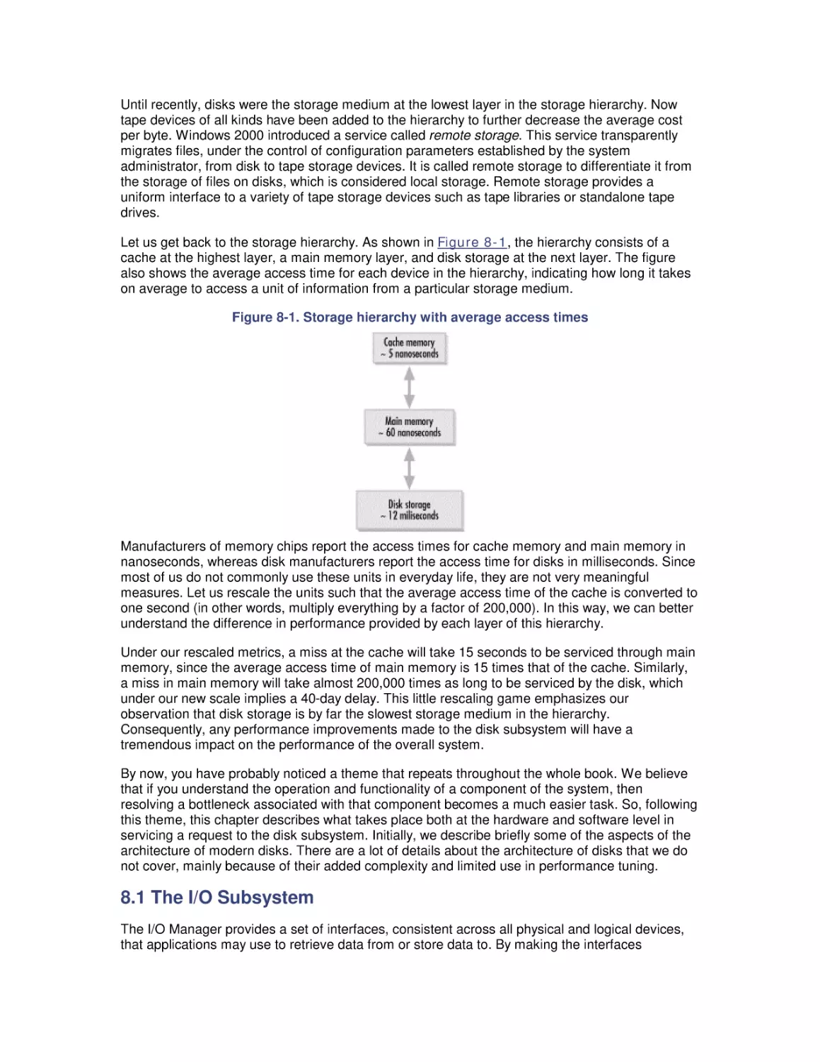
Chapter 8 introduces basic disk performance concepts.
Chapter 9 looks at filesystem performance.
Chapter 10 discusses the disk array technology used in most larger Windows 2000 servers.
Chapter 11 is a survey of computer networking, with an emphasis on the TCP/IP support in
Windows 2000.
Chapter 12 focuses on the Microsoft web server application Internet Information System (IIS).
The bibliography contains a list of references for those who would like to pursue these topics in
more depth.
Conventions Used in This Book
We have used the following conventions in this book:
•
Italic is used for filenames, directories, URLs, and hostnames. It is also used for
emphasis and to introduce new terms.
•
Constant width is used for commands, keywords, functions, and utilities.
•
Constant width italic is occasionally used for replaceable items in code.
This icon signifies a tip relating to the nearby text.
This icon signifies a warning relating to the nearby text.
How to Contact Us
Please address comments and questions concerning this book to the publisher:
O'Reilly & Associates, Inc.
1005 Gravenstein Highway North
Sebastopol, CA 95472
(800) 998-9938 (in the United States or Canada)
(707) 829-0515 (international or local)
(707) 829-0104 (fax)
We have a web page for this book, where we list errata and any additional information. You can
access this page at:
http://www.oreilly.com/catalog/w2kperf/
To comment or ask technical questions about this book, send email to:
bookquestions@oreilly.com
For more information about books, conferences, Resource Centers, and the O'Reilly Network,
see O'Reilly's web site at:
http://www.oreilly.com
Acknowledgments
Both authors gratefully acknowledge the support and assistance of Robert Denn and his staff at
O'Reilly, without whom the book you hold in your hands would never have been completed. We
are especially grateful for Robert's steady hand and patience throughout the long gestation period
for this book. At one point we thought that he might select an engraving of a sloth to adorn the
front cover. We would also like to acknowledge the help of many other individuals who reviewed
earlier drafts of the book, including Dave Butchart, Janet Bishop, Bob Gauthier, Todd Glasgow,
Kitrick Sheets, Jim Quigley, and Rich Olcott. They all contributed to making the final text clearer
and more readable. Any errors that remain are solely the responsibility of the authors.
Mark would like to acknowledge the support of Ziya Aral and George Teixiera of Datacore for
allowing him to complete this book on their watch. He is grateful for the long and fruitful
collaboration with Stets Newcomb, Phil Henninge, and Dave Steier, working out the details of the
Windows 2000 performance monitoring API. Special thanks to Joanne Decker for watching over
me during this period. Barry Merrill, in particular, was helpful in getting that project off the ground,
and his enthusiastic encouragement over the years is greatly appreciated. Russ Blake and Bob
Watson from Microsoft also provided valuable support and assistance when we were starting out.
Bob Gauthier, Jim Quigley, Sharon Seabaugh, Denis Nothern, and Claude Aron all contributed
useful ideas and practical experiences. Also, thanks to Jee Ping, Kitrick Sheets, Dave Solomon,
and Mark Russinovich for sharing their knowledge of Windows 2000 operating system internals.
Mark would also like to recognize some of the many individuals who contributed to his
understanding of the discipline of computer performance evaluation over the past twenty years of
his deepening involvement in the field. Alexandre Brandwajn and Rich Olcott deserve special
recognition for being stimulating collaborators over a long and fruitful period. Thanks to Jeff
Buzen, Pat Artis, Ken Sevcik, Barry Merrill, Dick Magnuson, Ben Duhl, and Phil Howard for all
nurturing my early interest in this subject. A belated thanks to Kathy Clark of Landmark Systems
for allowing me the opportunity to practice what I preached in the area of mainframe performance.
A nod to Bob Johnson for giving me the courage to even attempt writing a book in the first place
and to Bob Thomas for encouraging my writing career. To Bernie Domanski, Bill Fairchild, Dave
Halbig, Dan Kaberon, Chris Loosely, Bruce McNutt, Rich Milner, Mike Salsburg, Ray Wicks, Brian
Wong, and many other friends and colleagues too numerous to mention from the Computer
Measurement Group, I owe a debt of gratitude that I can never repay for having shared their
ideas and experiences so freely.
Thanks to the folks at Data General for giving us access to the CLARiiON disk array, and the
folks at 3Ware Corporation for letting Odysseas use their RAID adapters. Thanks also to Ed
Bouryng, Burton Strauss, Avi Tembulkar, and Michael Barker at KPMG for getting Odysseas
involved with their performance tuning effort.
Odysseas would like to thank Edward Lazowska, Kenneth Sevcik, and John Zahorjan, who got
him started in the area of performance modeling of computer systems with their summer course
at Stanford University. I appreciate the support of Yelena Yesha from the University of Maryland
at Baltimore County, and Milt Halem at NASA's Center for Computational Sciences, who got me
involved with modeling the performance of hierarchical mass storage systems and supported me
throughout that effort. Special thanks to Dr. Daniel Menasce of George Mason University for
taking me under his wing. Danny generously shared his extensive knowledge and experience in
the field of performance evaluation and modeling. He was also instrumental in honing my
technical writing and research skills.
I want to thank my mother and brothers for their love and support over the years. I owe sincere
gratitude to my father who always believed in me. If he were still alive, he would have been proud
to see this book. Last, but not least, I must extend my most sincere gratitude to my wife Yimin.
Throughout the long gestation period in getting this book completed, she took care of our two
wonderful kids, John and Sophia, while I disappeared down in the basement to finish that very
last chapter or make that very last modification. Despite the extra effort that she had to exert to
compensate for my absence, she was supportive throughout.
Chapter 1. Perspectives on Performance
Management
Our goal in writing this book is to provide a good introduction to the Windows 2000 operating
system and its hardware environment, focusing on understanding how it works from the
standpoint of a performance analyst responsible for planning, configuration, and tuning. Our
target audience consists of experienced performance analysts, system administrators, and
developers who are already familiar with the Windows 2000 operating system environment.
Taken as a whole, Windows 2000 performance involves not just the operating system, but also
the performance characteristics of various types of computer hardware, application software, and
communications networks. The key operating system performance issues include understanding
CPU scheduling and multiprogramming issues and the role and impact of virtual memory. Key
areas of hardware include processor performance and the performance characteristics of I/O
devices and other peripherals. Besides the operating system (OS), it is also important to
understand how the database management system (DBMS) and transaction-monitoring software
interact with both the OS and the application software and affect the performance of applications.
Network transmission speeds and protocols are key determinants of communication
performance. This is a lot of ground to cover in a single book, and there are many areas where
our treatment of the topic is cursory at best. We have compiled a rather lengthy bibliography
referencing additional readings in areas that we can discuss only briefly in the main body of this
book.
1.1 Windows 2000 Evolution
Before we start to describe the way Windows 2000 works in detail, let's summarize the evolution
of Microsoft's premier server operating system. While we try to concentrate on current NT
technology (i.e., Windows 2000), this book encompasses all current NT releases from Version 3.5
onward, including current versions of NT 4.0 and Windows 2000. Each succeeding version of
Windows NT incorporates significant architectural changes and improvements that affect the way
the operating system functions. In many cases, these changes impact the interpretation of
specific performance data counters, making the job of writing this book quite challenging.
Of necessity, the bulk of the book focuses on Windows 2000, with a secondary interest in
Windows NT 4.0, as these are the releases currently available and in wide distribution. We have
also had some experience running beta and prerelease versions of Windows XP. From a
performance monitoring perspective, the 32-bit version of XP appears quite similar to Windows
2000. The few remaining NT 3.51 machines we stumble across are usually stable production
environments running Citrix's WinFrame multiuser software that people are not willing to upgrade.
A daunting challenge to the reader who is familiar with some of the authoritative published works
on NT performance is understanding that what was once good solid advice has become obsolete
due to changes in the OS between Version 3, Version 4, and Windows 2000. Keeping track of the
changes in Windows NT since Version 3 and how these changes impact system performance
and tuning requires a little perspective on the evolution of the NT operating system, which is, after
all, a relatively new operating system. Our purpose in highlighting the major changes here is to
guide the reader who may be familiar with an older version of the OS. The following table
summarizes these changes.
New feature/change
Comment
Added/changed between
NT 3.5 and NT 4.0
New diskperf -ye option
Fix to monitor Physical Disk activity in a volume set or software
RAID 0/5 set correctly.
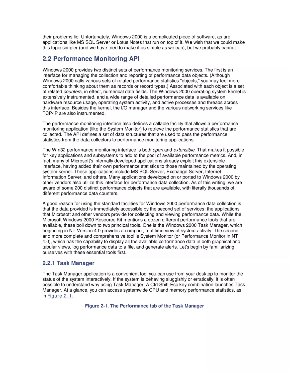
Task Manager performance
Makes it easier to find and kill looping programs.
tabs
Logical and Physical Disk
Avg Queue Length
Counters added
The % Disk Time Counters were mistakenly identified as measuring
disk utilization.
Revised Perfmon User
Guide documentation
Tones down extravagant claims that Windows NT is "self-tuning."
Symmetric (SMP)
Multiprocessor Support
NT Version 3 supports only asymmetric multiprocessing. All
interrupts are serviced on Processor 0. With SMPs, device driver
code must be made "thread-safe."
Common Network Device
Interface Specification
(NDIS) across Win9x and
Windows NT
As long as network card vendors have to rewrite NIC device drivers
anyway for Version 4, at least they will work on Windows 95, too.
Win32.dll
Moving user and GDI functions into the NT Executive provides better
Windows than Windows.
Added/changed between
NT 4.0 and Windows 2000
Many Sysmon enhancements, including fonts and multiple log data
Sysmon.OCX MMC snap-in
formats. Some valuable features inexplicably dropped, including the
replaces Perfmon
Chart Export facility.
Logical and Physical Disk 100% - Idle Time = disk utilization; mislabeled % Disk Time counters
% Idle Time counter added are retained.
Per Process I/O Counts
added to Task Manager
and Physical Disk objects
Requested by developers of analytic and simulation modeling
packages. Unfortunately, the Windows 2000 counters track logical
file requests, not necessarily correlated with Physical Disk activity.
New Printer Queue
measurements
Job Object with resource
limits introduced
Intended to provide a means for IIS to throttle runaway CGI scripts.
Windows Measurement
Instrumentation
Support for the WBEM standard. Provides an infrastructure for
integrated configuration, operations, and performance reporting
tools. Actually first introduced in NT 4.0 with Service Pack 4, but not
widely deployed.
New kernel Trace facility
Provides the ability to trace page faults, I/O requests, TCP requests,
and other low-level functions without hooking the OS.
_Total instance of the
Processor object
supersedes counters in
System object
Below Normal and Above
Normal Priority Levels
Provides more choice in the Scheduler's dynamic range.
Two choices for the
duration of the time-slice
Semantics behind Win32PrioritySeparation changed again! Choose
either Professional's short time slice interval or Server's very long
quantum.
interval.
Queued Spin Locks
enhance SMP scalability
Queued spin locks reduce internal processor bus contention
because threads do not have to execute a busy wait.
Network Monitor driver
replaces Network Monitor
Agent
The Network Monitor Agent placed the NIC in promiscuous mode in
order to capture packets for performance analysis. The new Network
Monitor driver looks only at packets processed by the networking
stack.
Integrated support for
Terminal Server Edition
(TSE)
WinFrame was developed independently by Citrix for Version 3.51.
After purchasing the rights from Citrix for version 4.0, TSE was
integrated on top of existing NT 4.0 service packs. Windows 2000
Terminal Server adds a new Session object. The User object in NT
4.0 TSE is dropped to maintain consistency.
Added/changed between
Windows 2000 and
Windows XP
64-bit Windows
16 TB virtual address space.
Intel SpeedStep
measurement support
Since processor MHz varies based on power source, processor time
is accumulated in separate buckets.
Process Heap Counters
Set DisplayHeapPerfObject to enable.
Volume Snapshot service
Filesystem support for cache flush and hold writes.
Faster boot and application
Uses Logical Disk prefetching.
launch
Writing a book on Windows 2000 performance is an interesting challenge. Many of the popular
computer books featured at your local bookstore promise easy answers. There is the Computers
for Dummies series, the Teach Yourself Windows 2000 in 30 Days style book, the bookshelf on
Windows 2000 Server Administration that looks like it was produced and sold by the pound, and
the one that promises that if you follow its expert recommendations you will never again have a
problem. We do not believe that giving simple solutions is the most effective way to communicate
ideas and issues relating to computer performance. We expect that readers of this book will likely
find themselves in difficult situations that have no direct precedent. In those situations, you will
have to fall back on the insight and knowledge of basic principles that we describe in this book.
Although we of coursedispense friendly advice from time to time, we concentrate instead on
providing the information and the conceptual framework designed to help you become your own
Windows 2000 performance expert.
1.2 Tools of the Trade
Understanding the tools of the performance analyst's trade is essential for approaching matters of
Windows 2000 performance. Rather than focus merely on tools and how they work, we chose to
emphasize the use of analytic techniques to diagnose and solve performance problems. We
stress an empirical approach, making observations of real systems under stress. If you are a
newcomer to the Microsoft operating system but understand how Unix, Linux, Solaris, OpenVMS,
MVS, or another full-featured OS works, you will find much that is familiar here. Moreover, despite
breathtaking changes in computer architecture, many of the methods and techniques used to
solve earlier performance problems can still be applied successfully today. This is a comforting
thought as we survey the complex computing environments, a jumbled mass of hardware and
software alternatives, that we are called upon to assess, configure, and manage today.
Measurement methodology, workload characterization, benchmarking, decomposition
techniques, and analytic queuing models remain as effective today as they were for the
pioneering individuals who first applied these methods to problems in computer performance
analysis.
Computer performance evaluation is significant because it is very closely associated with the
productivity of the human users of computerized systems. Efficiency is the principal rationale for
computer-based automation. Whenever productivity is a central factor in decisions regarding the
application of computer technology to automate complex and repetitive processes, performance
considerations loom large. These concerns were present at the dawn of computing and remain
very important today. Even as computing technology improves at an unprecedented rate, the fact
that our expectations of this technology grow at an even faster rate assures that performance
considerations will continue to be important in the future.
In computer performance, productivity is often tangled up with cost. Unfortunately, the
relationship between performance and cost is usually neither simple nor straightforward.
Generally, more expensive equipment has better performance, but there are many exceptions.
Frequently, equipment will perform well with some workloads but not others. In most buying
decisions, it is important to understand the performance characteristics of the hardware, the
performance characteristics of the specific workload, and how they match up with each other.
In a sea of change, computer performance is one of the few areas of computing to remain
relatively constant. As computing paradigms shift, specific areas of concern to performance
analysts are subject to adjustment and realignment. Historically, the central server model of
mainframe computing was the focus of much performance analysis in the 1960s and early 1970s.
Understanding the performance of timesharing systems with virtual memory motivated basic
research. Today, the focus has shifted to the performance of client/server applications, two- and
three-tiered architectures, web-enabled transaction processing applications, internetworking,
electronic mail and other groupware applications, databases, and distributed computing.
Windows 2000 is at the center of many of these trends in desktop, networking, and enterprise
computing, which is why Windows 2000 performance remains a critical concern.
1.2.1 Performance Measures
To be able to evaluate the performance of a computer system, you need a thorough
understanding of the important metrics used to measure computer performance. Computers are
machines designed to perform work, and we measure their capacity to perform the work, the rate
at which they are currently performing it, and the time it takes to perform specific tasks. In the
following sections, we look at some of the key ways to measure computer performance,
introducing the most commonly used metrics: bandwidth, throughput, service time, utilization, and
response time.
1.2.1.1 Bandwidth
Bandwidth measures the capacity of a link, bus, channel, interface, or device to transfer data. It is
usually measured in either bits/second or bytes/second (there are eight bits in a data byte). For
example, the bandwidth of a 10BaseT Ethernet connection is 10 Mb/sec, the bandwidth of a
SCSI-2 disk is 20 MB/sec, and the bandwidth of the PCI Version 2.1 64-bit 66 MHz bus is 528
MB/sec.
Bandwidth usually refers to the maximum theoretical data transfer rate of a device under ideal
conditions, and, therefore, it needs to be treated as an upper bound of performance. You can
rarely measure the device actually performing at that rate, as there are many reasons why the
theoretical bandwidth is not achievable in real life. For instance, when an application transfers a
block of information to the disk, various layers of the operating system (OS) normally need to
process the request first. Also, before a requested block of data can be transferred across a
channel to the disk, some sort of handshaking protocol is required to set up the hardware
operation. Finally, at the physical disk itself, your request is likely to be delayed during the time it
takes to position the read/write actuator of the disk over the designated section on the rotating
magnetic platter. The unavoidable overhead of operating system software, protocol message
exchange, and disk positioning absorbs some of the available bandwidth so the application
cannot use the full rated bandwidth of the disk for data transfer.
To provide another example, in networking people are accustomed to speaking about the
bandwidth of a LAN connection to transfer data in millions of bits per second. Consider an
application that seeks to transfer an IP packet using the UDP protocol on an Ethernet network.
The actual packet, when it reaches your network hardware, looks like Figure 1-1, with additional
routing and control information added to the front of the message by various networking software
layers.
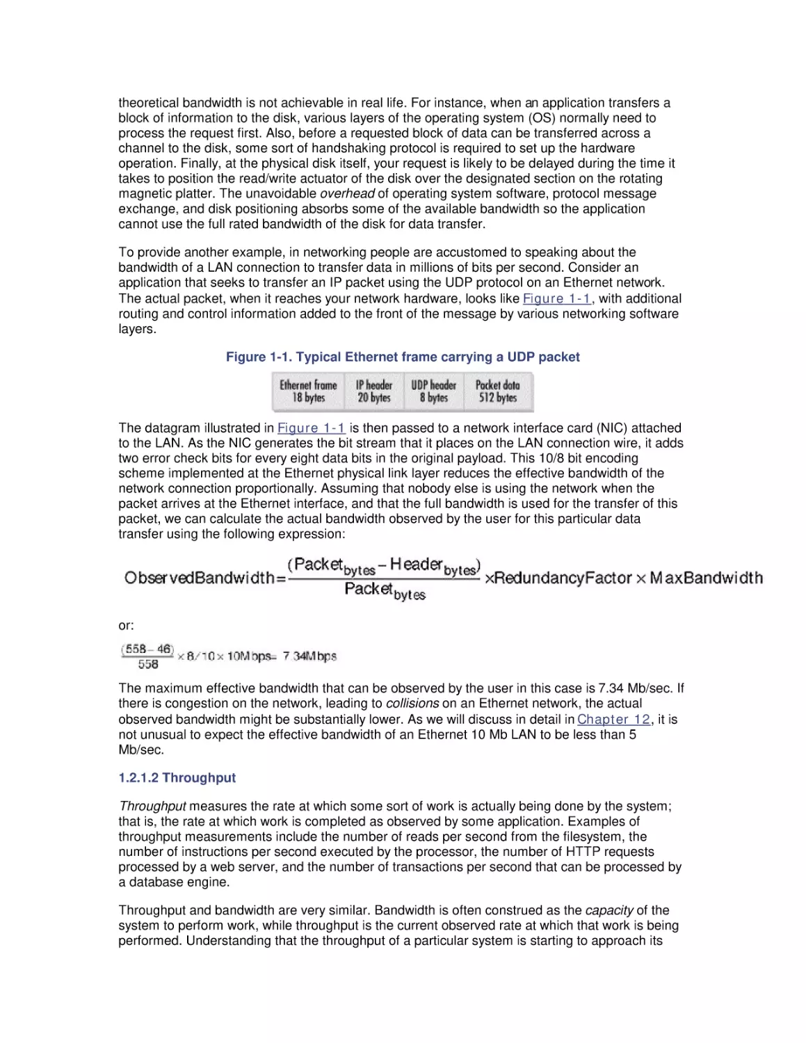
Figure 1-1. Typical Ethernet frame carrying a UDP packet
The datagram illustrated in Figure 1-1 is then passed to a network interface card (NIC) attached
to the LAN. As the NIC generates the bit stream that it places on the LAN connection wire, it adds
two error check bits for every eight data bits in the original payload. This 10/8 bit encoding
scheme implemented at the Ethernet physical link layer reduces the effective bandwidth of the
network connection proportionally. Assuming that nobody else is using the network when the
packet arrives at the Ethernet interface, and that the full bandwidth is used for the transfer of this
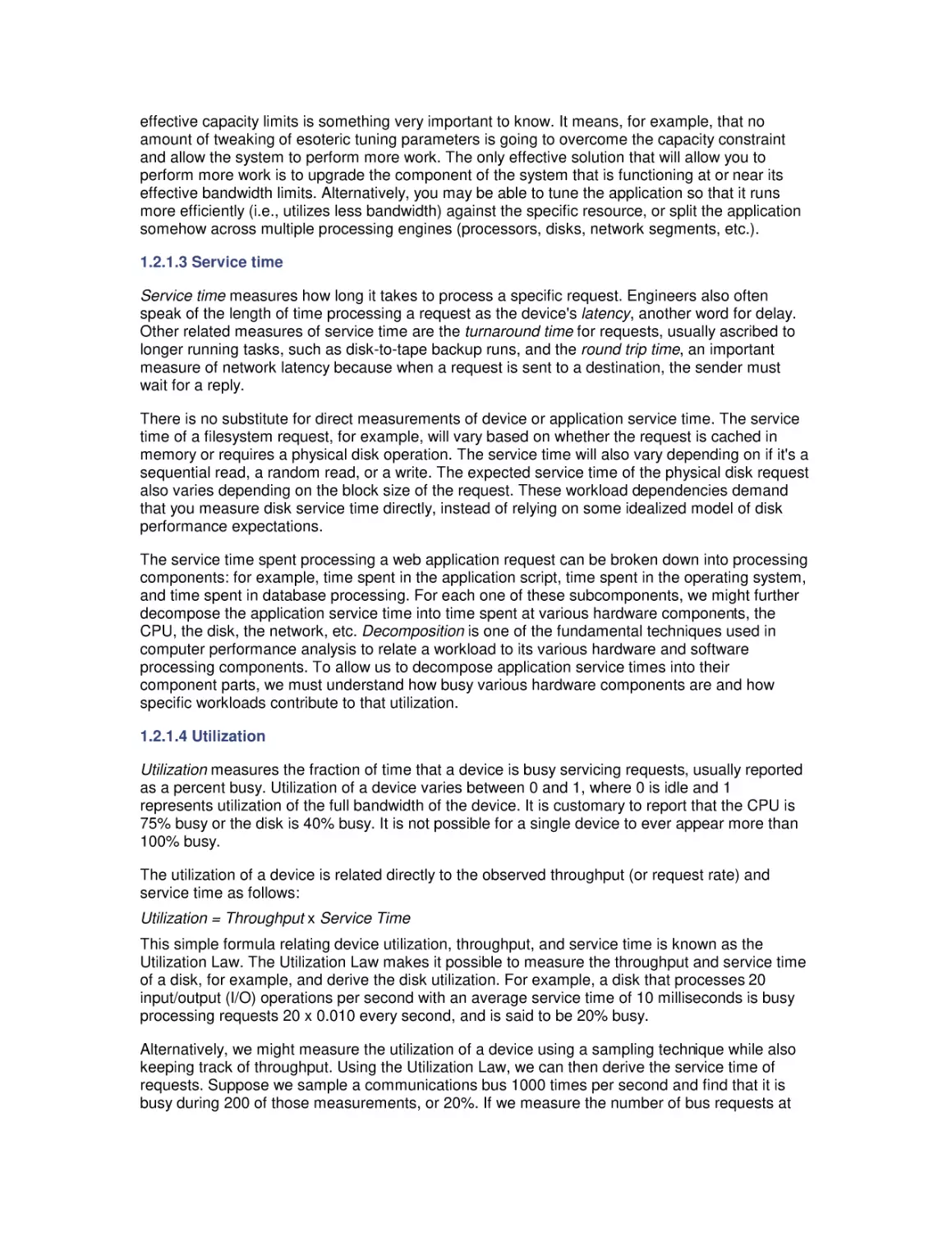
packet, we can calculate the actual bandwidth observed by the user for this particular data
transfer using the following expression:
or:
The maximum effective bandwidth that can be observed by the user in this case is 7.34 Mb/sec. If
there is congestion on the network, leading to collisions on an Ethernet network, the actual
observed bandwidth might be substantially lower. As we will discuss in detail in Chapter 12, it is
not unusual to expect the effective bandwidth of an Ethernet 10 Mb LAN to be less than 5
Mb/sec.
1.2.1.2 Throughput
Throughput measures the rate at which some sort of work is actually being done by the system;
that is, the rate at which work is completed as observed by some application. Examples of
throughput measurements include the number of reads per second from the filesystem, the
number of instructions per second executed by the processor, the number of HTTP requests
processed by a web server, and the number of transactions per second that can be processed by
a database engine.
Throughput and bandwidth are very similar. Bandwidth is often construed as the capacity of the
system to perform work, while throughput is the current observed rate at which that work is being
performed. Understanding that the throughput of a particular system is starting to approach its
effective capacity limits is something very important to know. It means, for example, that no
amount of tweaking of esoteric tuning parameters is going to overcome the capacity constraint
and allow the system to perform more work. The only effective solution that will allow you to
perform more work is to upgrade the component of the system that is functioning at or near its
effective bandwidth limits. Alternatively, you may be able to tune the application so that it runs
more efficiently (i.e., utilizes less bandwidth) against the specific resource, or split the application
somehow across multiple processing engines (processors, disks, network segments, etc.).
1.2.1.3 Service time
Service time measures how long it takes to process a specific request. Engineers also often
speak of the length of time processing a request as the device's latency, another word for delay.
Other related measures of service time are the turnaround time for requests, usually ascribed to
longer running tasks, such as disk-to-tape backup runs, and the round trip time, an important
measure of network latency because when a request is sent to a destination, the sender must
wait for a reply.
There is no substitute for direct measurements of device or application service time. The service
time of a filesystem request, for example, will vary based on whether the request is cached in
memory or requires a physical disk operation. The service time will also vary depending on if it's a
sequential read, a random read, or a write. The expected service time of the physical disk request
also varies depending on the block size of the request. These workload dependencies demand
that you measure disk service time directly, instead of relying on some idealized model of disk
performance expectations.
The service time spent processing a web application request can be broken down into processing
components: for example, time spent in the application script, time spent in the operating system,
and time spent in database processing. For each one of these subcomponents, we might further
decompose the application service time into time spent at various hardware components, the
CPU, the disk, the network, etc. Decomposition is one of the fundamental techniques used in
computer performance analysis to relate a workload to its various hardware and software
processing components. To allow us to decompose application service times into their
component parts, we must understand how busy various hardware components are and how
specific workloads contribute to that utilization.
1.2.1.4 Utilization
Utilization measures the fraction of time that a device is busy servicing requests, usually reported
as a percent busy. Utilization of a device varies between 0 and 1, where 0 is idle and 1
represents utilization of the full bandwidth of the device. It is customary to report that the CPU is
75% busy or the disk is 40% busy. It is not possible for a single device to ever appear more than
100% busy.
The utilization of a device is related directly to the observed throughput (or request rate) and
service time as follows:
Utilization = Throughput x Service Time
This simple formula relating device utilization, throughput, and service time is known as the
Utilization Law. The Utilization Law makes it possible to measure the throughput and service time
of a disk, for example, and derive the disk utilization. For example, a disk that processes 20
input/output (I/O) operations per second with an average service time of 10 milliseconds is busy
processing requests 20 x 0.010 every second, and is said to be 20% busy.
Alternatively, we might measure the utilization of a device using a sampling technique while also
keeping track of throughput. Using the Utilization Law, we can then derive the service time of
requests. Suppose we sample a communications bus 1000 times per second and find that it is
busy during 200 of those measurements, or 20%. If we measure the number of bus requests at
2000 per second over the same sampling interval, we can derive the average service time of bus
requests equal to 0.2 — 2000 = .0001 seconds or 100 microseconds (
secs).
Monitoring the utilization of various hardware components is an important element of capacity
planning. Measuring utilization is very useful in detecting system bottlenecks, which are
essentially processing constraints due to limits on the effective throughput capacity of some
overloaded device. If an application server is currently processing 60 transactions per second
with a CPU utilization measured at 20%, the server apparently has considerable reserve capacity
to process transactions at an even higher rate. On the other hand, a server processing 60
transactions per second running at a CPU utilization of 98% is operating at or near its maximum
capacity.
Unfortunately, computer capacity planning is not as easy as projecting that the server running at
20% busy processing 60 transactions per second is capable of processing 300 transactions per
second. You would not need to read a big, fat book like this one if that were all it took. Because
transactions use other resources besides the CPU, one of those other resources might reach its
effective capacity limits long before the CPU becomes saturated. We designate the component
functioning as the constraining factor on throughput as the bottlenecked device. Unfortunately, it
is not always easy to identify the bottlenecked device in a complex, interrelated computer system
or network of computer systems.
It is safe to assume that devices observed operating at or near their 100% utilization limits are
bottlenecks, although things are not always that simple. For one thing, 100% is not necessarily
the target threshold for all devices. The effective capacity of an Ethernet network normally
decreases when the utilization of the network exceeds 40-50%. Ethernet LANs use a shared link,
and packets intended for different stations on the LAN can collide with one another, causing
delays. Because of the way Ethernet works, once line utilization exceeds 40-50%, collisions start
to erode the effective capacity of the link. We will talk about this phenomenon in much more detail
in Chapter 11.
1.2.1.5 Response time
As the utilization of shared components increases, processing delays are encountered more
frequently. When the network is heavily utilized and Ethernet collisions occur, for example, NICs
are forced to retransmit packets. As a result, the service time of individual network requests
increases. The fact that increasing the rate of requests often leads to processing delays at busy
shared components is crucial. It means that as we increase the load on our server from 60
transactions per second and bottlenecks in the configuration start to appear, the overall response
time associated with processing requests will not hold steady. Not only will the response time for
requests increase as utilization increases, it is likely that response time will increase in a
nonlinear relationship to utilization. In other words, as the utilization of a device increases slightly
from 80% to 90% busy, we might observe that the response time of requests doubles, for
example.
Response time, then, encompasses both the service time at the device processing the request
and any other delays encountered waiting for processing. Formally, response time is defined as:
Response time = service time + queue time
where queue time represents the amount of time a request waits for service. In general, at low
levels of utilization, there is minimal queuing, which allows device service time to dictate response
time. As utilization increases, however, queue time increases nonlinearly and, soon, begins to
dominate response time.
Queues are essentially data structures where requests for service are parked until they can be
serviced. Examples of queues abound in Windows 2000, and measures showing the queue
length or the amount of time requests wait in the queue for processing are some of the most
important indicators of performance bottlenecks discussed here. The Windows 2000 queues that
will be discussed in this book include the operating system's thread scheduling queue, the logical
and physical disk queues, the file server request queue, and the queue of Active Server Pages
(ASP) web server script requests. Using a simple equation known as Little's Law, which is
discussed later, we will also show how the rate of requests, the response time, and the queue
length are related. This relationship, for example, allows us to calculate average response times
for ASP requests even though Windows 2000 does not measure the response time of this
application directly.
In performance monitoring, we try to identify devices with high utilizations that lead to long
queues where requests are delayed. These devices are bottlenecks throttling system
performance. Intuitively, what can be done about bottlenecks once you have discovered one?
Several forms of medicine can be prescribed:
•
Upgrade to a faster device
•
Spread the workload across multiple devices
•
Reduce the load on the device by tuning the application
•
Change scheduling parameters to favor cherished workloads
These are hardly mutually exclusive alternatives. Depending on the situation, you may wish to try
more than one of them. Common sense dictates which alternative you should try first. Which
change will have the greatest impact on performance? Which configuration change is the least
disruptive? Which is the easiest to implement? Which is possible to back out of in case it makes
matters worse? Which involves the least additional cost? Sometimes, the choices are fairly
obvious, but often these are not easy questions to answer.
One complication is that there is no simple relationship between response time and device
utilization. In most cases it is safe to assume the underlying relationship is nonlinear. A peer-topeer Ethernet LAN experiencing collisions, for example, leads to sharp increases in both network
latency and utilization. A Windows 2000 multiprocessor implementing priority queuing with
preemptive scheduling at the processor leads to a categorically different relationship between
response time and utilization, where low-priority threads are subject to a condition called
starvation. A SCSI disk that supports tagged command queuing can yield higher throughput with
lower service times at higher request rates. In later chapters, we explore in much more detail the
performance characteristics of the scheduling algorithms that these hardware devices use, each
of which leads to a fundamentally different relationship between utilization and response time.
This nonlinear relationship between utilization and response time often serves as the effective
capacity constraint on system performance. Just as customers encountering long lines at a fast
food restaurant are tempted to visit the fast food chain across the way when delays are palpable,
customers using an Internet connection to access their bank accounts might be tempted to switch
to a different financial institution if it takes too long to process their requests. Consequently,
understanding the relationship between response time and utilization is one of the most critical
areas of computer performance evaluation. It is a topic we will return to again and again in the
course of this book.
Response time measurements are also important for another reason. For example, the response
time for a web server is the amount of time it takes from the instant that a client selects a
hyperlink to the time that the requested page is returned and displayed on her display monitor.
Because it reflects the user's perspective, the overall response time is the performance measure
of greatest interest to the users of a computer system. It is axiomatic that long delays cause user
dissatisfaction with the computer systems they are using, although this is usually not a
straightforward relationship either. Human factors research, for instance, indicates that users may
be more bothered by unexpected delays than by consistently long response times that they have
become resigned to.
1.2.2 Optimizing Performance
Intuitively, it may seem that proper configuration and tuning of any computer system or network
should attempt to maximize throughput and minimize response time simultaneously. In practice,
that is often not possible. For example, system administrators that try to optimize throughput are
apt to drive up response time to unacceptable levels as a result. Alternatively, minimizing
response time by stockpiling only the fastest and most expensive equipment and then keeping
utilization low in order to minimize queuing delays is not very cost-effective. In practice, skilled
performance analysts attempt to achieve a balance between these often conflicting objectives:
•
There is relatively high throughput leading to the cost-effective use of the hardware.
•
Queuing delays are minimal, so users are satisfied with performance levels.
•
System performance is relatively stable, consistent, and predictable.
To explain that these objectives are not so easy to reconcile, it may help to take an introductory
look at queuing theory, a branch of operations research frequently applied to the analysis of
computer systems performance.
1.2.2.1 Single-server model
Figure 1-2 shows the conventional representation of a queuing system, with customer requests
arriving at a server with a simple queue. These are the basic elements of a queuing system:
customers, servers, and a queue. Figure 1-2 shows a single server, but multiple-server models
are certainly possible.
Figure 1-2. Simple model of a queuing system showing customer requests arriving at a
single server
If the server is idle, customer requests arriving at the server are processed immediately. On the
other hand, if the server is already busy, then the request is queued. If multiple requests are
waiting in the server queue, the queuing discipline determines the order in which queued
requests are serviced. The simplest and fairest way to order the queue is to service requests in
the order in which they arrive. This is also called FIFO (First In, First Out) or sometimes First
Come, First Served (FCFS). There are many other ways that a queue of requests can be
ordered, including by priority or by the speed with which they can be processed.
1.2.2.2 Modeling assumptions
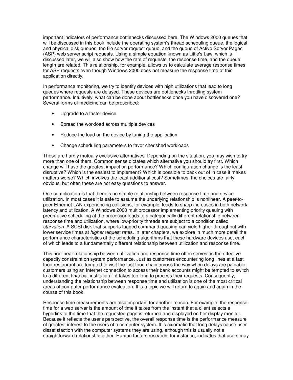
Figure 1-3 shows a simple queue annotated with symbols that represent a few of the more
common parameters that define its behavior. There are a large number of parameters that can be
used to describe the behavior of this simple queue, and we only look at a couple of the more
basic and commonly used ones. Response time (W) represents the total amount of time a
customer request spends in the queuing system, including both service time (W s) at the device
and wait time (W q) in the queue. By convention, the Greek letter (lambda) is used to specify
the arrival rate or frequency of requests to the server. Think of the arrival rate as an activity rate
such as the rate at which HTTP GET requests arrive at a web server, I/O requests are sent to a
disk, or packets are sent to a NIC card. Larger values of
indicate that a more intense workload
, is
is applied to the system, whereas smaller values indicate a light load. Another Greek letter,
used to represent the rate at which the server can process requests. The output from the server
is either or
, whichever is less, because it is certainly possible for requests to arrive at a
server faster than they can processed.
Figure 1-3. A queuing model with its parameters
Ideally, we hope that the arrival rate is lower than the service rate of the server, so that the server
can keep up with the rate of customer requests. In that case, the arrival rate is equal to the
completion rate, an important equilibrium assumption that allows us to consider models that are
mathematically tractable (i.e., solvable). If the arrival rate
is greater than the server capacity
, then requests begin backing up in the queue. Mathematically, arrivals are drawn from an
)
infinite population so that when >
, the queue length and the wait time (Wq at the server
grow infinitely large. Those of us who have tried to retrieve a service pack from a Microsoft web
server immediately after its release know this situation and its impact on performance.
Unfortunately, it is not possible to solve a queuing model with >
, although mathematicians
have developed heavy traffic approximations to deal with this familiar case.
In real-world situations, there are limits on the population of customers. The population of
customers in most realistic scenarios involving computer or network performance is limited by the
number of stations on a LAN, the number of file server connections, the number of TCP
connections a web server can support, or the number of concurrent open files on a disk. Even in
the worst bottlenecked situation, the queue depth can only grow to some predetermined limit.
When enough customer requests are bogged down in queuing delays, in real systems, the arrival
rate for new customer requests becomes constrained. Customer requests that are backed up in
the system choke off the rate at which new requests are generated.
The purpose of this rather technical discussion is twofold. First, it is necessary to make an
unrealistic assumption about arrivals being drawn from an infinite population to generate readily
solvable models. Queuing models break down when
, which is another way of saying
they break down near 100% utilization of some server component. Second, you should not
confuse a queuing model result that shows a nearly infinite queue length with reality. In real
systems there are practical limits on queue depth. In the remainder of our discussion here, we will
assume that <
. Whenever the arrival rate of customer requests is equal to the completion
rate, this can be viewed as an equilibrium assumption. Please keep in mind that the following
results are invalid if the equilibrium assumption does not hold; in other words, if the arrival rate of
requests is greater than the completion rate (
queuing models do not work.
>
over some measurement interval) simple
1.2.2.3 Little's Law
A fundamental result in queuing theory known as Little's Law relates response time and
utilization. In its simplest form, Little's Law expresses an equivalence relation between response
time W, arrival rate
queue length):
Q=
, and the number of customer requests in the system Q (also known as the
xW
Note that in this context the queue length Q refers both to customer requests in service (Qs) and
waiting in a queue (Qq) for processing. In later chapters we will have several opportunities to take
advantage of Little's Law to estimate response time of applications where only the arrival rate and
queue length are known. Just for the record, Little's Law is a very general result that applies to a
large class of queuing models. While it does allow us to estimate response time in a situation
where we can measure the arrival rate and the queue length, Little's Law itself provides no insight
into how response time is broken down into service time and queue time delays.
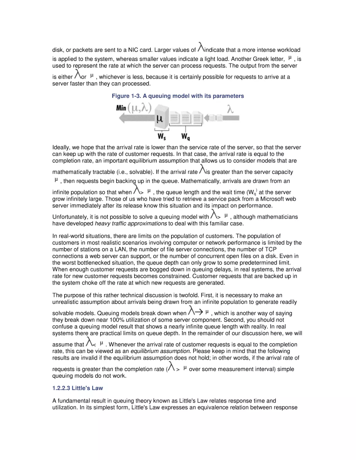
Little's Law is an important enough result that it is probably worth showing how to derive it. As
mentioned, Little's Law is a very general result in queuing theory± only the equilibrium
assumption is required to prove it. Figure 1-4 shows some measurements that were made at
disk at discrete intervals shown on the X axis. The Y axis indicates the number of disk requests
during the interval. Our observation of the disk is delimited by the two arrows between the start
time and the stop time. When we started monitoring the disk, it was idle. Then, whenever an
arrival occurred at a certain time, we incremented the arrivals counter. That variable is plotted
using the thick line. Whenever a request completed service at the disk, we incremented the
completions variable. The completions are plotted using the thin line.
Figure 1-4. A graph illustrating the derivation of Little's Law
The difference between the arrival and completion lines is the number of requests at the disk at
that moment in time. For example, at the third tick-mark on the X axis to the right of the start
arrow, there are two requests at the disk, since the arrival line is at 2 and the completion line is at
0. When the two lines coincide, it means that the system is idle at the time, since the number of
arrivals is equal to the number of departures.
To calculate the average number of requests in the system during our measurement interval, we
need to sum the area of the rectangles formed by the arrival and completion lines and divide by
the measurement interval. Let's define the more intuitive term "accumulated time in the system"
for the sum of the area of rectangles between the arrival and completion lines, and denote it by
the variable P. Then we can express the average number of requests at the disk, N, using the
expression:
We can also calculate the average response time, R, that a request spends in the system (Ws +
W q) by the following expression:
where C is the completion rate (and C = , from the equilibrium assumption). This merely says
that the overall time that requests spent at the disk (including queue time) was P, and during that
time there were C completions. So, on average, each request spent P/C units of time in the
system.
Now, all we need to do is combine these two equations to get the magical Little's Law:
Little's Law says that the average number of requests in the system is equal to the product of the
rate at which the system is processing the requests (with C = , from the equilibrium
assumption) times the average amount of time that a request spends in the system.
To make sure that this new and important law makes sense, let's apply it to our disk example.
Suppose we collected some measurements on our system and found that it can process 200
read requests per second. The Windows 2000 System Monitor also told us that the average
response time per request was 20 ms (milliseconds) or 0.02 seconds. If we apply Little's Law, it
tells us that the average number of requests at the disk, either in the queue or actually in
processing, is 200 x 0.02, which equals 4. This is how Windows 2000 derives the Physical Disk
Avg. Disk Queue Length and Logical Disk Avg. Disk Queue Length counters. More on that topic
in Chapter 8.
The explanation and derivation we have provided for Little's
Law is very intuitive and easy to understand, but it is not
100% accurate. A more formal and mathematically correct
proof is beyond the scope of this book. We followed the
development of Little's Law and notation used by a classic
book on queuing networks by Lazowska, Zahorjan, Graham,
and Sevcik called Quantitative System Performance:
Computer System Analysis Using Queuing Network Models.
This is a very readable book that we highly recommend if you
have any interest in analytic modeling. Regardless of your
interest in mathematical accuracy, though, you should
become familiar with Little's Law. There are occasions in this
book where we use Little's Law to either verify or improve
upon some of the counters that are made available in
Windows 2000 through the System Monitor. Even if you
forget everything else we say here about analytic modeling,
don't forget the formula for Little's Law.
1.2.2.4 M/M/1
For a simple class of queuing models, the mathematics to solve them is also quite simple. A
simple case is where the arrival rate and service time are randomly distributed around the
average value. The standard notation for this class of model is M/M/1 (for the single-server case)
and M/M/n (for multiple servers). M/M/1 models are useful because they are easy to compute±
not necessarily because they model reality precisely. We can derive response time for an M/M/1
or M/M/n model with FIFO queuing if the arrival rate and service time are known using the
following simple formula:
where u is the utilization of the server, W q is the queue time, W s is the service time, and W q + W s
= W. As long as we remember that this model breaks down as utilization approaches 100%, we
can use it with a fair degree of confidence.
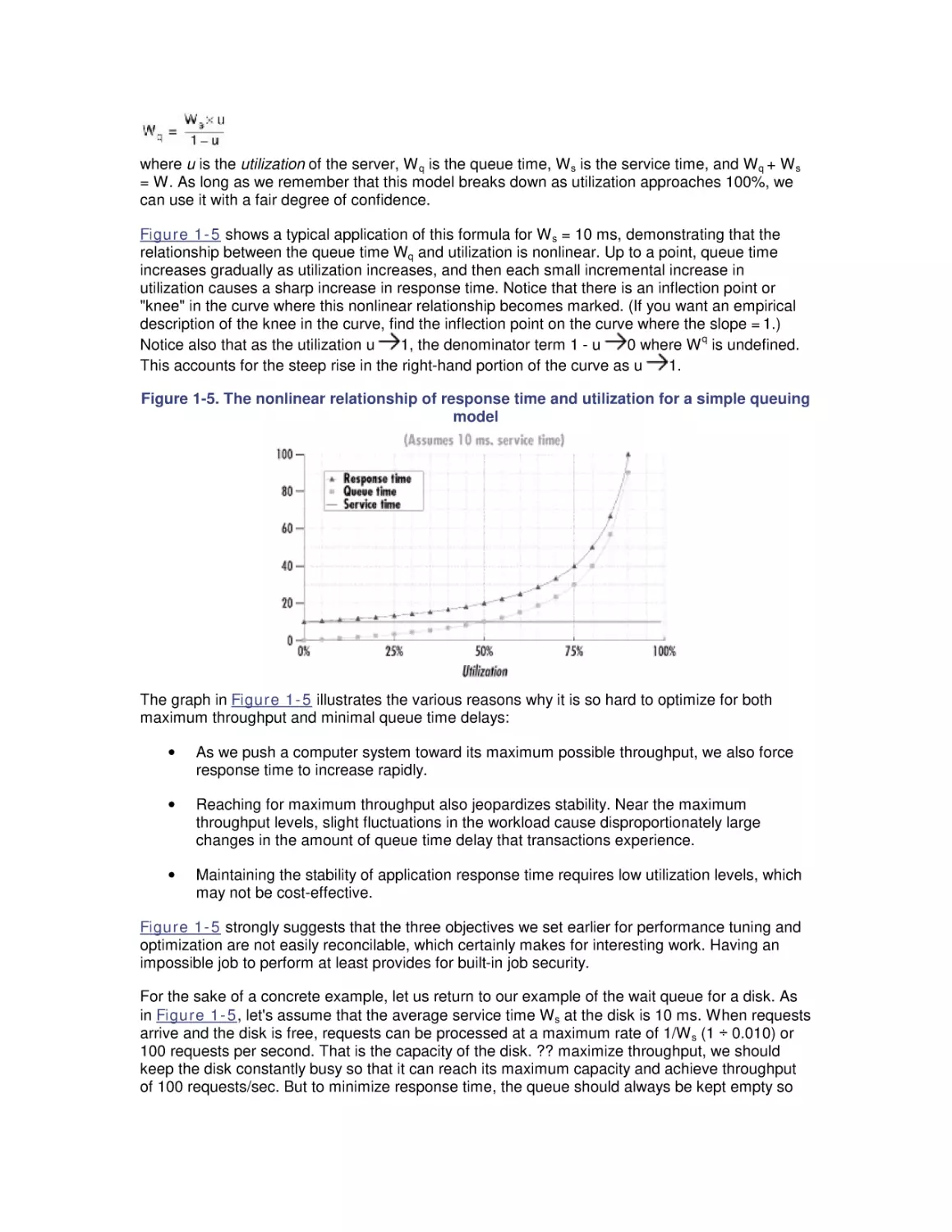
Figure 1-5 shows a typical application of this formula for W s = 10 ms, demonstrating that the
relationship between the queue time Wq and utilization is nonlinear. Up to a point, queue time
increases gradually as utilization increases, and then each small incremental increase in
utilization causes a sharp increase in response time. Notice that there is an inflection point or
"knee" in the curve where this nonlinear relationship becomes marked. (If you want an empirical
description of the knee in the curve, find the inflection point on the curve where the slope = 1.)
q
Notice also that as the utilization u
1, the denominator term 1 - u
0 where W is undefined.
This accounts for the steep rise in the right-hand portion of the curve as u
1.
Figure 1-5. The nonlinear relationship of response time and utilization for a simple queuing
model
The graph in Figure 1-5 illustrates the various reasons why it is so hard to optimize for both
maximum throughput and minimal queue time delays:
•
As we push a computer system toward its maximum possible throughput, we also force
response time to increase rapidly.
•
Reaching for maximum throughput also jeopardizes stability. Near the maximum
throughput levels, slight fluctuations in the workload cause disproportionately large
changes in the amount of queue time delay that transactions experience.
•
Maintaining the stability of application response time requires low utilization levels, which
may not be cost-effective.
Figure 1-5 strongly suggests that the three objectives we set earlier for performance tuning and
optimization are not easily reconcilable, which certainly makes for interesting work. Having an
impossible job to perform at least provides for built-in job security.
For the sake of a concrete example, let us return to our example of the wait queue for a disk. As
in Figure 1-5, let's assume that the average service time Ws at the disk is 10 ms. When requests
arrive and the disk is free, requests can be processed at a maximum rate of 1/W s (1 — 0.010) or
100 requests per second. That is the capacity of the disk. ?? maximize throughput, we should
keep the disk constantly busy so that it can reach its maximum capacity and achieve throughput
of 100 requests/sec. But to minimize response time, the queue should always be kept empty so
that the total amount of time it takes to service a request is as close to 10 milliseconds as
possible.
If we could control the arrival of customer requests (perhaps through scheduling) and could time
each request so that one arrived every W s seconds (once every 10 ms), we would improve
performance. When requests are paced to arrive regularly every 10 milliseconds, the disk queue
is always empty and the request can be processed immediately. This succeeds in making the
disk 100% busy, attaining its maximum potential throughput of 1/Ws requests per second. With
perfect scheduling and perfectly uniform service times for requests, we can achieve 100%
utilization of the disk with no queue time delays.
In reality, we have little or no control over when I/O requests arrive at the disk in a typical
computer system. In a typical system, there are periods when the server is idle and others when
requests arrive in bunches. Moreover, some requests are for large amounts of data located in a
distant spot on the disk, while others are for small amounts of data located near the current disk
actuator. In the language of queuing theory, neither the arrival rate distribution of customer
requests or the service time distribution is uniform. This lack of uniformity causes some requests
to queue, with the further result that as the throughput starts to approach the maximum possible
level, significant queuing delays occur. As the utilization of the server increases, the response
time for customer requests increases significantly during periods of congestion, as illustrated by
the behavior of the simple M/M/1 queuing model in Figure 1-5. [1]
[1]
The simple M/M/1 model we discuss here was chosen because it is simple, not because it is necessarily
representative of real behavior on live computer systems. There are many other kinds of queuing models
that reflect arrival rate and service time distributions different from the simple M/M/1 assumptions. However,
although M/M/1 may not be realistic, it is easy to calculate. This contrasts with G/G/1, which uses a general
arrival rate and service time distribution, i.e., any kind of statistical distribution: bimodal, symptomatic, etc.
No general solution to a G/G/1 model is feasible, so computer modelers are often willing to compromise
reality for solvability.
1.2.3 Queuing Models in Theory and Practice
This brief mathematical foray is intended to illustrate the idea that attempting to optimize
throughput while at the same time minimizing response is inherently difficult, if not downright
impossible. It also suggests that any tuning effort that makes the arrival rate or service time of
customer requests more uniform is liable to be productive. It is no coincidence that this happens
to be the goal of many popular optimization techniques. It further suggests that a good approach
to computer performance tuning and optimization should stress analysis, rather than simply
dispensing advice about what tuning adjustments to make when problems occur.
We believe that the first thing you should do whenever you encounter a performance problem is
to measure the system experiencing the problem and try to understand what is going on.
Computer performance evaluation begins with systematic empirical observations of the systems
at hand.
In seeking to understand the root cause of many performance problems, we rely on a
mathematical approach to the analysis of computer systems performance that draws heavily on
insights garnered from queuing theory. Ever notice how construction blocking one lane of a threelane highway causes severe traffic congestion during rush hour? We may notice a similar
phenomenon on the computer systems we are responsible for when a single component
becomes bottlenecked and delays at this component cascade into a problem of major
proportions. Network performance analysts use the descriptive term storm to characterize the
chain reaction that sometimes results when a tiny aberration becomes a bigproblem. Long before
chaos theory, it was found that queuing models of computer performance can accurately depict
this sort of behavior mathematically. Little's Law predicts that as utilization of a resource
increases linearly, response time increases exponentially. This fundamental nonlinear
relationship that was illustrated in Figure 1-5 means that quite small changes in the workload
can result in extreme changes in performance indicators, especially as important resources start
to become bottlenecks.
This is exactly the sort of behavior you can expect to see in the computer systems you are
responsible for. Most computer systems do not degrade gradually. Queuing theory is a useful tool
in computer performance evaluation because it is a branch of mathematics that models systems
performance realistically. The painful reality we face is that performance of the systems we are
responsible for is acceptable day after day, until quite suddenly it goes to hell in a handbasket.
This abrupt change in operating conditions often begets an atmosphere of crisis. The typical
knee-jerk reaction is to scramble to identify the thing that changedand precipitated the
emergency. Sometimes it is possible to identify what caused the performance degradation, but
more often it is not so simple.
With insights from queuing theory, we learn that it may not be a major change in circumstances
that causes a major disruption in current performance levels. In fact, the change can be quite
small and gradual and still produce a dramatic result. This is an important perspective to have the
next time you are called upon to diagnose a Windows 2000 performance problem. Perhaps the
only thing that changed is that a component on the system has reached a high enough level of
utilization where slight variations in the workload provoke drastic changes in behavior.
A full exposition of queuing theory and its applications to computer performance evaluation is well
beyond the scope of this book. Readers interested in pursuing the subject might want to look at
Daniel Mensace's Capacity Planning and Performance Modeling: From Mainframes to
Client/Server Systems; Raj Jain's encyclopedic The Art of Computer Systems Performance
Analysis: Techniques for Experimental Design, Measurement, Simulation, and Modeling; or
Arnold Allen's very readable textbook on Probability, Statistics, and Queuing Theory With
Computer Science Applications.
1.2.4 Exploratory Data Analysis
Performance tuning presupposes some form of computer measurement. Understanding what is
measured, how measurements are gathered, and how to interpret them is another crucial area of
computer performance evaluation. You cannot manage what you cannot measure, but
fortunately, measurement is pervasive. Many hardware and software components support
measurement interfaces. In fact, because of the quantity of computer measurement data that is
available, it is often necessary to subject computer usage to some form of statistical analysis.
This certainly holds true on Windows 2000, which can provide large amounts of measurement
data. Sifting through all these measurements demands an understanding of a statistical approach
known as exploratory data analysis, rather than the more familiar brand of statistics that uses
probability theory to test the likelihood that a hypothesis is true or false. John Tukey's classic
textbook entitled Exploratory Data Analysis (currently out of print) or Understanding Robust and
Exploratory Data Analysis by Hoaglin, Mosteller, and Tukey provides a very insightful introduction
to using statistics in this fashion.
Many of the case studies described in this book apply the techniques of exploratory data analysis
to understanding Windows 2000 computer performance. Rather than explore the copious
performance data available on a typical Windows 2000 platform at random, however, our search
is informed by the workings of computer hardware and operating systems in general, and of
Windows 2000, Intel processor hardware, SCSI disks, and network interfaces in particular.
Because graphical displays of information are so important to this process, aspects of what is
known as scientific visualization are also relevant. (It is always gratifying when there is an
important-sounding name for what you are doing!) Edward Tufte's absorbing books on scientific
visualization, including Visual Explanations and The Visual Display of Quantitative Information,
are an inspiration.[2] In many place in this book, we will illustrate the discussion with exploratory
data analysis techniques. In particular, we will look for key relationships between important
measurement variables. Those illustrations rely heavily on visual explanations of charts and
graphs to explore key correlations and associations. It is a technique we recommend highly.
[2]
It is no surprise that Professor Tufte is extending Tukey's legacy of the exploratory data analysis
approach, as Tukey is a formative influence on his work.
In computer performance analysis, measurements, models, and statistics remain the tools of the
trade. Knowing what measurements exist, how they are taken, and how they should be
interpreted is a critical element of the analysis of computer systems performance. We will address
that topic in detail in Chapter 2, so that you can gain a firm grasp of the measurement data
available in Windows 2000, how it is obtained, and how it can be interpreted.
1.3 Performance and Productivity
As mentioned at the outset, there is a very important correlation between computer performance
and productivity, and this provides a strong economic underpinning to the practice of performance
management. Today, it is well established that good performance is an important element of
human-computer interface design. (See Ben Schneiderman's Designing the User Interface:
Strategies for Effective Human-Computer Interaction.) We have to explore a little further what it
means to have "good" performance, but systems that provide fast, consistent response time are
generally more acceptable to the people who use them. Systems with severe performance
problems are often rejected outright by their users and fail. This leads to costly delays, expensive
rewrites, and loss of productivity.
1.3.1 The Transaction Model
As computer performance analysts, we are interested in finding out what it takes to turn "bad"
performance into "good" performance. Generally, the analysis focuses on two flavors of computer
measurements. The first type of measurement data describes what is going on with the hardware,
operating systems software, and application software that is running. These measurements
reflect both activityrates and the utilization of key hardware components: how busy the processor,
the disks, and the network are. Windows 2000 provides a substantial amount of performance
data in this area: quantitative information on how busy different hardware components are, what
processes are running, how much memory they are using, etc.
The second type of measurement data measures the capacity of the computer to do productive
work. As discussed earlier in this chapter, most common measures of productivity we have seen
are throughput (usually measured in transactions per second) and response time. A measure of
throughput describes the quantity of work performed, while response time measures how long it
takes to complete the task. When users of your network complain about bad performance, you
need a way to quantify what "bad" is. You need application response time measurements from
the standpoint of the end user. Unfortunately, Windows 2000 is not very strong in this key area of
measurement.
To measure the capacity of the computer to do productive work, we need to:
•
Characterize end user interactions in identifiable units of work
•
Measure and report how long it takes for the computer to process these units of work
Then, computer performance analysts try to determine why these processes are running slowly,
and figure out how to speed things up. Sounds pretty simple, doesn't it?
There is an implicit assumption that computer processing can be broken into identifiable units for
analysis when we talk about the performance and tuning of computer processing workloads in
this fashion. Conceptually, we are using what is known as the transaction model. Transactions
are atomic units of processing± you cannot break a transaction down into anything smaller
without losing whatever it is that makes it a transaction. A transaction might involve executing
SQL statements to query a database, applying a special effect in an image-processing program,
scrolling a word-processing document from its beginning to the point where you left off editing, or
recalculating a column of figures in a spreadsheet. These are all recognizable units of processing
with a definite beginning and end. A transaction corresponds to some specific action that a user
takes to initiate work. This correspondence is the critical link between the transaction response
time and user productivity.
Let's look at some of the ways in which the transaction model is relevant to computer
performance analysis. The performance of different configurations can be calibrated accurately
by running any of the recognized industry benchmark streams that measure computer and
network throughput, usually in transactions per second (or TPS). TPS is a common measure of
throughput that is accepted across the industry. It is also possible to relate computer throughput
to end user productivity, namely, how long it takes an individual to accomplish some computerassisted task. Once we know how long it takes to process transactions, it may then be possible to
determine what components are taking the most time (decomposition), why processing takes so
long (bottleneck analysis), and what can be done to improve it (prescriptive tuning). These three
analysis techniques are of fundamental importance, and we will revisit them many times in this
book.
The transaction model also lends itself to the mathematical techniques associated with queuing
theory. The two main elements of a queuing system are:
•
A set of transaction-oriented workloads
•
Networks of servers and queues
Many types of queuing systems can be analyzed mathematically if the arrival rate of transactions
and their service demands are known. The theoretical model referred to back in Figure 1-3, for
example, is based on very simple assumptions about the average rate in which new transactions
are generated and the processing demands of these transactions.
Unfortunately, it is not always easy to group processing activities into distinct transactions in
Windows 2000. An application running in the foreground (with the active title bar) processes
mouse moves and keyboard events on a more or less continuous basis. It is hard to tell where a
particular transaction begins or ends under these circumstances. Where work is not easily
grouped into transactions, Windows 2000 does not measure and report transaction response
time. In other cases, defining the boundaries of transactions is less problematic. In a client/server
model, the point where the client application accesses a database on the server could easily
mark the beginning of a transaction. When the server application finishes all its processing on
behalf of the client request and returns control to the client application, the transaction is
considered complete. An update transaction will issue a Commit command when it is finished
processing, an unambiguous marker of the end of the transaction. If you are running client/server
applications based on MS Exchange, MS SQL Server, or the Microsoft Transaction Server, it is
possible to organize workloads into transaction units. It is disappointing that while these
subsystems keep some transaction-oriented performance statistics, they generally do not report
response time systematically.
Experienced performance analysts sorely miss having adequate transaction response time data
to work with in Windows 2000. Without it, it is not possible to relate all the measurements about
what is going on inside the computer to the work that people are doing with the computer. This
complicates performance analysis, and it means that some of the best, proven methods cannot
easily be applied to Windows 2000.
1.3.2 Designing for Performance
From the standpoint of an application developer, it is important to understand how to deliver
software that performs well. A common fallacy is to measure system response time and equate it
to productivity. While the two are related, they are far from the same thing. Consider a computer
reservation system used by a trained operator. One implementation might break the task of
making a reservation down into several subtasks, each of which is implemented to execute
quickly. However, because the interaction with the computer requires a series of transactions, the
actual process of making a reservation is long and complex. A second implementation might
collapse all the user interactions into a single, more complicated transaction. It might take longer
to process the bulkier transaction than several smaller transactions combined. According to
objective measures of transaction response time, the first system is the better one. It is also the
system people are apt to like better because it provides fast, consistent response. It just feels
better.
Productivity is another matter. In this instance, productivity is measured as the number of
reservations per day a skilled operator can perform. Under the second system, users may
actually be able to perform more work, as measured objectively in reservations made per day per
operator. The second system may also be cheaper to operate than the first because it does not
process quite so many transactions, and it may even be able to support a heavier reservation
load. Because workers are more productive using the second system, the company does not
need quite so many operators and can be more profitable. User satisfaction with the second
system, however, is probably somewhat lower than with the first alternative, presuming that it is
possible to reduce these subjective feelings to an objective, quantitative scale.
Which system do you think your company will want to use? Which system do you think you would
like to use? It is important to understand that any large-scale application system that you design
and deliver is subject to very restrictive cost and performance constraints. All parties to the
application development process, including the end user, must understand what these limitations
are and accept them as reasonable.
If satisfaction is in the eye of the beholder, as a software developer you should look for ways to
improve the performance of the second system to make it more acceptable. Perhaps procuring
more expensive hardware can be justified. Alternately, there may be things that can be done to
the design of the second system to make it more user-friendly without actually speeding it up. The
psychological aspects of human-computer interaction are outside the scope of the book, but this
is an area that experienced software designers should know something about. There are many
simple design techniques and tricks that can make systems more palatable even when they are
not lightning-fast.
Tricks of the Trade
Experienced application developers use many tricks to make long waits
more acceptable to their users. For example, a status bar that provides
feedback to a user is a friendlier way to process a long-running
transaction than leaving the user in the dark about how long it will take.
Status bars that estimate how long something like a file transfer will take
are effective, but only if the prediction is halfway in the ballpark. The best
technique is to make an estimate of the whole job based on the rate at
which your program completes the first part of it, and update the estimate
based on current activity rates.
While inexperienced users appreciate an application wizard that takes
them through a new process step by step, experienced users are likely to
find the extra steps tedious and annoying. Typically, you ne ed to satisfy
both groups. New users want to learn an application easily, without
having to read the manual, and become productive quickly. Experienced
users want the ability to execute complex, repetitive tasks quickly and
easily. For inexperienced users, one approach is to provide wizards that
walk them through a new task step by step. Meanwhile, experienced
users need shortcuts like the macro-level ability to combine several
commands into a new one, limiting the amount of user interaction
required to perform command sequences that are executed repetitively.
Another programming trick is useful when there is a long processing
delay, for example, when you are opening a file or retrieving a large
number of records from a database. This trick is to display pa rtial results
as soon as you can while continuing with the long-running process in the
background. This is a little trickier to program because you need to
spawn a separate thread to process the long-running task in the
background, and learn how to signal across threads running
asynchronously. Inside the worker thread, be sure to communicate back
to the main thread when you have accumulated enough data to display
the first screen. Then, signal the main thread when the retrieval process
has completed and terminate the worker thread if it is no longer needed.
This trick exploits the difference between computer time and human
interaction time to make your application look more responsive than it
actually is.
1.4 Performance Management
Performance management remains one of the key system management disciplines performed by
systems professionals of all stripes. For instance, as a LAN administrator, you may be
responsible for setting up the hardware platform and operating system environment used to run
the applications that your company needs to run its business. The performance aspects of this
job include monitoring the hardware and software and making configuration changes and tuning
adjustments to make things run better. To support capacity planning and budgeting, you may be
called upon to provide measurement data to cost-justify hardware expenditures and as input to
the capacity planning process that is designed to ensure that adequate resources continue to be
available.
In a capacity planning role, you may be responsible for assuring that adequate resources are
available over the long term. This may mean monitoring the current growth, factoring in new
application projects, and trying to plan the hardware configuration that can supply adequate
performance. This inevitably means that you will encounter your company's budget for new
equipment purchases. You will be called upon to explain your recommendations in
straightforward, nontechnical language. Perhaps your analysis will show that more hardware is
needed to meet the performance objectives or else workers interacting with the system will not be
fully productive. This is part of performance management, too.
Our approach to these and other performance management tasks is decidedly empirical.
Remember, you cannot manage what you cannot measure. We recommend that you gather data
from real systems in operation, analyze it, and make decisions based on that analysis. Those
decisions may range from deciding how to configure a workstation running Windows 2000
Professional for optimal performance for a graphics-intensive application, to how to configure
multiple Windows 2000 servers to support distributed database or messaging applications. For
systems under development, you may need to discuss hardware and software infrastructure
alternatives with the programmers responsible for implementing the application. If you get an
opportunity to influence the design of an important application under development, try to link
decisions about design trade-offs to actual measurements of prototype code running under
different conditions of stress. Before setting parameters and making tuning adjustments, review
and analyze performance statistics from the system. Afterwards, verify that the changes you
made are working by looking at similar measurement data.
Whatever the challenge, your approach should always be analytical. For example, before making
a tuning adjustment, analyze the measurement data and develop a working hypothesis as to what
the problem is and how to solve it. You will rely on a variety of analytical tools, mainly queuing
models and statistical analysis. The analysis generates a working hypothesis, which is then
tested against further observations. Does the adjustment you made improve the system's
behavior in the way you expected? That is often convincing evidence that the working hypothesis
you adopted was an appropriate one.
1.4.1 Rules of Thumb (ROTs)
The empirical approach we recommend contrasts with something we will call the Rule of Thumb
approach. Rules of thumb (ROTs) are received wisdom passed down from professed experts to
the masses. This sounds like a great approach since these self-appointed wizards appear to
know much more about the sacred innards of Windows 2000 than you do. The problem with
these pearls of wisdom is that they may not apply to your specific environment. We think you
should find out how these great seers derived the rule being espoused, attempt to apply the same
derivation to your environment, and determine for yourself if the rule is applicable. Quite possibly,
after you have modified the rule to your specific environment, it may very well be relevant to your
situation.
For example, our approach to evaluating whether or not to do a memory upgrade begins with the
hypothesis that the amount of paging is related to an index of memory utilization we can
calculate. The difference between a Windows 2000 server configured at 256 MB versus one
configured at 512 MB might be a significant amount of money. If multiple Windows 2000 servers
or workstations are involved, the dollars start to add up fast. The memory utilization index you
need to calculate is the number of committed virtual memory bytes divided by the amount of
hardware RAM installed. Look to find empirical evidence in the performance measurements that a
relationship exists between the memory utilization index and paging activity. If this relationship
does exist and you understand its behavior, you may be able to use it to estimate the benefits of
a memory upgrade. This particular technique is discussed in greater detail in Chapter 6.
If we know that this relationship exists on many different systems, we might then distill the
evidence into a general configuration rule. Without much further analysis, we might suggest that a
good configuration rule of thumb is to provide at least 1 MB of RAM for every 2 MB of committed
virtual memory. This is a very easy rule to apply because you can simply run the Task Manager
application and access the Performance tab to determine the Commit Charge (K) total virtual
memory peak (see Figure 1-6). Divide the Commit Charge (K) total by the Physical Memory (K)
total field. If that ratio is 2 or more, it may be time to buy more memory for that machine.
Remember, however, that your mileage may vary. Rather than just blindly applying this rule, we
want you to understand how the rule was derived and be capable of adapting the method to your
particular set of circumstances. We will discuss the empirical evidence used to derive this rule in
Chapter 6, and try to explain how you can test to see whether this rule will work for you.
Figure 1-6. Task Manager Performance tab
1.4.2 Is Performance Tuning Obsolete?
Before proceeding further, there is a common notion that needs to be dispelled. This is the belief
that performance considerations in the design and development of computer applications no
longer matter because computing resources are so inexpensive. Advocates of this position
concede that there may be a few instances where performance is still an important consideration
today, but if you just wait a couple more years, these problems will be solved as the hardware
keeps getting faster and cheaper.
We have heard this claim that "performance doesn't matter anymore" for at least 10 years, and
we do not believe it is any truer today than it was a decade ago. First, though, we should admit
that our perspective is warped because we are frequently the "outside expert" who is called in
only during a crisis. Most people do not call the fire department until they have a fire. So we tend
to see extreme situations where people are desperate for a solution and do not know where else
to turn. Amazingly, many of these problems are very easy to diagnose and can often be solved
right over the phone. On the other hand, some problems take weeks and months worth of effort to
solve. And some of them, we are sorry to say, are never resolved to everyone's satisfaction.
(There is a joke that no one ever said computer science was an exact science.) Seeing only the
more extreme cases tends to warp your perspective. However, we do see just as many of these
problems today that we did ten years ago, so it does not seem reasonable to believe bigger and
better hardware has solved all our performance problems. Computer performance is still a topic
worthy of your consideration.
On the other hand, it is certainly true that the strides taken to improve the performance of
hardware have been phenomenal. The PC that sits on our desktop today is a splendid piece of
equipment. It costs considerably less money than you would have paid for a 640K PC/XT just 15
years ago. It has five hundred times more memory and about thousand times more disk space. It
is lightning-fast at most tasks (although it is still painfully slow at others). Yes, hardware is
improving rapidly, but it is important to realize that not all hardware advances at the same rate.
For example, advances in disk performance have not been as rapid as instruction processing
speeds. Moreover, even as the hardware gets cheaper and cheaper, there are always
applications that demand even more resources than we have available.
In addition, computer performance continues to have a cost dimension to it that remains very
significant. Many aspects of hardware design reflect cost/performance trade-offs, and it's
important to understand what these are. A software developer still needs to understand how
algorithms perform and especially how they scale as the problem space becomes larger or more
users are added to the system. Finished designs for any nontrivial system are always
compromises that aim for the best balance between performance and cost.
1.4.3 Bottleneck Analysis
To make the best planning decisions, a traditional approach is to try and understand hardware
speeds and feeds -- how fast different pieces of equipment are capable of running. This is much
more difficult than it sounds. For example, it certainly seems like a SCSI disk attached to a 20
MB/second SCSI-2 adapter card should run much slower than one attached to an 80 MB/second
UltraSCSI-3 adapter card. UltraSCSI-3 sounds as if should beat ol' SCSI-2 every time. But there
may be little or no practical difference in the performance of the two configurations. (Perhaps the
disk may only transfer data at 20 MB/second anyway, so the extra capacity of the UltraSCSI-3
bus is not being utilized.)
This example illustrates the principle that a complex system will run only as fast as its slowest
component. Because there is both theory and extensive empirical data to back up this claim, we
don't mind propagating this statement as a good rule of thumb. In fact, it provides the theoretical
underpinning for a very useful analysis technique, which we will call bottleneck analysis. The
slowest device in a configuration is often the weakest link. Find it and replace it with a faster
component and you have a good chance that performance will improve. Sounds good, but you
probably noticed that the rule does not tell you howto find this component. Given the complexity
of many modern computer networks, this seemingly simple task is as easy as finding a needle in
the proverbial haystack. Of course, replace some component other than the bottleneck device
with a faster component and performance will remain the same.
In both theory and practice, performance tuning is the process of locating the bottleneck in a
configuration and removing it. The system's performance will improve until the next bottleneck is
manifest, which you again identify and remove. Removing the bottlenecked device usually entails
replacing it with a newer, faster version of the same component. For example, if network
bandwidth is a constraint on performance, upgrade the configuration from 10 Mb Ethernet to 100
Mb Fast Ethernet. If the network actually is the bottleneck, performance should improve.
A system in which all bottlenecks have been removed can be said to be a balanced system. All
components in a balanced system are at least capable of handling the flow of work from
component to component without delays building up at any one particular component. Visualize a
network of computing components where work flows from one component (the CPU) to another
(the disk), back again, then to another (the network), and back again to the CPU (see Figure 17). When different components are evenly distributed across the hardware, that system is
balanced. It can even be proved mathematically that performance is optimal when a system is
balanced in this fashion.
Figure 1-7. A network of computing components and their queues
We can visualize that the balanced system (and not one that is simply over-configured) is one
where workload components are evenly distributed across the processing resources. If there are
delays, the work that is waiting to be processed is also evenly distributed in the system. This work
is illustrated by the shaded areas in Figure 1-8. Suppose we could crank up the rate at which
requests arrive to be serviced (think of SQL Server requests to a Windows 2000 database server,
for example, or logon requests to an Active Directory authentication server). If the system is
balanced, we will observe that work waiting to be processed remains evenly distributed around
the system as in Figure 1-8, but there is more of a backlog of requests that need distributing.
Figure 1-8. A balanced system where shaded areas indicate work queued for processing at
different hardware components
If instead we observe something like Figure 1-9, where many requests are waiting behind just
one of the resources, we can then say with some authority that that component isthe bottleneck in
the configuration. When work backs up behind a bottlenecked device, delays there may cascade,
causing delays elsewhere in the configuration. Because the flow of work through the system is
not a simple chain of events, but an interconnected network, the way that the delayed work
impacts processing at other components may not always be obvious. Empirically, it is sufficient to
observe that work accumulates behind the bottlenecked device at faster rates as the workload
increases. Replacing this component with a faster one should improve the rate that work can flow
through the entire system. So now you know that "computer performance analyst" is just a fancy
term for a computer plumber who goes around clearing stopped-up drains!
Figure 1-9. An unbalanced system where the second disk is the bottlenecked device
1.4.4 Benchmarking
Unfortunately for us computer plumbers, it is not always easy to figure out where bottlenecks are
or how to relieve them. Consider the nightly backup process that copies new and updated files to
tape so that you can restore a user's environment when a hard disk crashes. Assume that when
you first began backing up files on the computers attached to the LAN to the tape drive attached
to the backup server, the process took only four hours each night. Over time, because there are
more users and more disks, the process takes longer and longer. Soon there are not enough
hours during the evening to back up all the files that need to be backed up. What should be done
about this situation?
First, you upgrade the tape drive to a newer model that the manufacturer promises is faster and
more powerful. But that does not speed up the process. It is time to begin a search for the
bottlenecked device. Unfortunately, there are many potential devices to be considered. Perhaps
network bandwidth is the problem, and you need to update hubs, routers, and network interface
cards. Perhaps the network is adequate (utilization is low and there are few collisions), but the
network cards cannot pump data onto the line fast enough. Perhaps the cards are fine, but the
networking software is slowing things down by waiting too long before transmitting the next
request. (Maybe the TCP window size is not set correctly.) Perhaps the cards and the networking
software are fine, but the client CPU is not able to push data out to the card because the internal
bus connecting the card to the computer is not fast enough. Perhaps the hard disk where the files
reside simply cannot move the data any faster because files are spread all over the disk instead
of being located contiguously (i.e., the disk is fragmented). Perhaps this is not a problem that you
are going to solve tonight.
Once you find irrefutable evidence of a bottlenecked device, you want to replace it with a faster
component. How do we know that one component is actually faster than another? Will it actually
be faster when it comes to your workload? Unfortunately, these questions are not easy to answer
either. Worse, there is no general agreement or universally accepted standards of comparison
among different machines, platforms, and architectures. This is due to the fact that there are so
many workload-dependent factors. This leads us inevitably to the topic of building and executing
comparative benchmarks.
Benchmarks are repeatableexecution sequences that can be run on different computers at
different times to form a basis of comparison. A benchmarking methodology is as follows.
Develop a representative workload that can be executed over and over again. Run the workload
on System A and again on System B (which is configured differently) and compare the results.
Working hypothesis: Since the execution runs are otherwise identical, any time differences should
be a function of differences in the operating environments. A benchmark establishes an applesto-apples comparison between the performance of two or more systems.
Generally, there are two types of benchmark workloads: realand synthetic. Real (or natural)
benchmark workloads are created by capturing actual system usage with a tool that is later used
to play back the workload at a controlled rate or with more users. Synthetic benchmarks are
sample applications or programs that you acquire purely for testing purposes. The fact that these
synthetic applications exist and can be purchased off the shelf is particularly useful when the
capacity planning exercise is for an application that remains to be built.
1.4.4.1 Benchmark applicability
The popularity of the benchmark approach, especially the test results reported extensively in
consumer-oriented trade publications, should not be confused with its effectiveness in making
configuration decisions. Decision-making based on benchmarks results, even with so-called
industry-standard benchmarks, almost always generates serious questions about validity and
interpretation. One important consideration is determining that the benchmark is relevant to the
kind of work you eventually plan to perform. The fact that the benchmark load, in the case of both
real or synthetic benchmarks, is representative of actual workloads is difficult to establish in
practice, and once established, is subject to change over time. How can you determine that a
given benchmark load is representative of your actual workload? Unfortunately, this is not a
question with a simple answer.
Another problem is the assumption that the benchmark is repeatable across many different
platforms. You are likely to find that benchmark measurements vary greatly in successive runs on
the same configuration. Various cache loading effects are notorious in this regard, and cache
techniques are in widespread use. (This is an enormously complicated technical topic that we will
pursue in Chapter 6 and Chapter 7.) Manufacturers typically provide speed ratings of their
equipment running standard benchmark suites in their development labs. When you attempt to
measure performance levels in your own environment, inevitably they suffer by comparison. This
leads immediately to the question, "What is different about my environment?" Again, not an easy
question to answer. In the case of benchmark results published in the trade press, you may not
be able to find out enough about the test configuration to ever make an apples-to-apples
comparison to your workload.
1.4.4.2 Benchmark repeatability
These additional elements make benchmarking much more complicated in practice than in
theory. Assessing the relative performance of two different processor architectures ought to be as
simple as running the same benchmark test against each and evaluating the results. It isn't. Raw
processor performance is typically measured by clock speed and the number of clock cycles
needed per instruction. This leads to a standard measure of instructions executed per second
(IPS) or Instruction Execution Rate (IER). But which instructions? Reduced Instruction Set
Computers (RISC) may require three instructions to perform the same logical operation that a
Complex Instruction Set Computer (CISC) can perform in one instruction. Both RISC and CISC
computers typically also have pipelines and scalar processing facilities that enable them to
execute some, but not all, instruction in parallel. Measurements of actual instruction execution
rates vary significantly from workload to workload depending on the instruction mix.
By comparison, measurements of disk speed are relatively standardized. Disks are usually
measured in terms of head seek time, rotational delay waiting to locate the desired sector while
the device spins, and data transfer rates in bytes per second. However, under benchmark testing
conditions, actual disk performance is affected by file placement, disk caching strategies, disk
fragmentation, and many other considerations. Network access primarily depends on the speed
of the wire, but is complicated by processing delays that occur as packets traverse the network of
connections between local area and wide area segments. The network protocol in use also
determines how many different messages are sent and received and what sorts of
acknowledgments are required. In most realistic circumstances, network topology is so unique
that only measurements gathered from the actual running system are trustworthy.
1.4.4.3 Benchmark engineering
Benchmarks are useful, but be careful in interpreting the results (the widely hyped test scores and
ratings in articles and advertisements notwithstanding). Remember, for any of the popular,
standardized benchmarks in widespread use, there is also a good deal of benchmark engineering
going on back at the factory. The engineers that developed the equipment tested it constantly by
running standard benchmarks to see if the latest engineering change yielded any improvement.
This is standard practice. Vendors need ways to stress test products under development, and
they naturally want to be able to advertise that their equipment received a better score than a
competitor's on a well-known benchmark test.
Frequently, engineers will insert optimizations designed to speed up execution running a specific
benchmark. The result of this process is equipment that is very good at running standard
benchmark workloads, but may not be so good at running yours. There is nothing wrong with this
practice, so long as the benchmark is in fact representative of actual workloads. But it does raise
issues of interpretation. There is always the possibility that a particular optimization that accounts
for a good benchmark score is not especially useful when it comes to your configuration and
workload.
The ideal situation is performing empirical testing with the equipment running your workload. But
building a realistic and representative benchmark-testing environment of your own is both
expensive and time-consuming. Nor can you test all the different varieties and configuration
permutations under consideration. Here, analytic techniques are useful for projecting the
performance of proposed configurations from actual performance measurements. Understanding
what the characteristics of the benchmark workload are and how they compare to your actual
workloads is crucial in performing this type of analysis. Workload characterization is an essential
first step in the analysis of both real and synthetic workloads.
1.5 Problems of Scale
As fast as hardware is improving, it still cannot always meet user expectations. Computer
applications are growing more intelligent and easier to use. However, because of this, they also
require more resources to run. Additionally, computer applications are being deployed to more
and more people living in every part of the world. This inevitably leads to problems of scale:
applications may run all right in development, but run in fits and starts when you start to deploy
them on a widespread basis.
Problems of scalability are some of the most difficult that application developers face. There are
three facets to scalability:
•
The problems computers must solve get characteristically more difficult to compute as
the number of elements involved grows.
•
People often have unrealistically high expectations about what computer technology can
actually do.
•
There are sometimes absolute physical constraints on performance that cannot be
avoided. This applies to long-distance telecommunications as much as it does to signal
propagation inside a chip or across a communications bus.
We discuss these three factors in the following sections.
1.5.1 Software Scalability
There are "hard" problems for computers that have a way of getting increasingly more
complicated as the problem space itself grows larger. A classic example is the traveling salesman
problem, where the computer calculates the most efficient route through multiple cities. This can
be accomplished by brute force with a small number of cities, for example, by generating all the
possible routes. As the number of cities increases, however, the number of possible routes the
computer must generate and examine increases exponentially. In the mathematics of computing,
these problems are known as NP-complete. With many NP-complete problems, as the problem
space grows more complicated, the computational effort using known methods explodes far
beyond what even the fastest computers can do.
An application such as a search engine for the Internet provides a good example of something
that works fine with a certain amount of data but collapses under the impact of more and more
data points. No doubt, at one point in time, search engines seemed like a wonderful way to
navigate the World Wide Web. Today, searching for web pages related to "Computer
Performance" on AltaVista, we found 3000+ matches. Meanwhile, on Northern Lights we found
13,000+ matches. On Lycos we found matches with almost 9,000 web sites. Frankly, we are not
sure whether it is better to find 3000 matches or 13,000; we certainly do not have time to look
through thousands of search engine entries. Clearly, search engine technology has trouble
dealing with the current scale of the Internet.
Commercial data processing workloads encounter similar problems of scalability. For example, it
is well known that sorting algorithms, a staple of commercial workloads, scale exponentially.
Building very large database applications that can scale to high volumes of activity and large
numbers of users is also challenging, but in a different way. The performance issues that affect
scalability in database and transaction processing workloads typically involve serialization and
locking. When one transaction updates the database, the portions of the database affected by the
update are locked. Other transactions that attempt to access the same portion of the database
are delayed until the update completes. Updates can cause powerful parallel processing modes
to revert back to much slower serial ones.
The implications of serialization and locking in the database world are very complicated. One
update may trigger further activity when the indexes that speed access to the data themselves
require updating. To ensure data integrity, certain update transactions may be forced to hold
locks for long periods of time until several different portions of the database are updated.
Database locking and serialization problems can typically be addressed only at the design stage.
As an aside, when programmers attempt to use rapid application development (RAD) and other
prototyping tools to speed the development process, transaction processing applications are
often prone to these problems of scale. Using these development tools, the application is
described in a logical fashion and then generated without regard to performance considerations.
The application will demo well on a low volume of data, but user expectations are later shattered
when the prototype does not scale beyond a small number of users, and the entire project then
has to be rewritten by hand in C++.
1.5.2 Unrealistic User Expectations
The second aspect of the current application development environment that leads to performance
problems is that expectations about what computer technology can and cannot do are often far
removed from reality. It does not help that these inflated expectations are fueled by vendor claims
of breakthroughs in applications such as handwriting analysis, speech recognition, and natural
language processing. These are all activities that require years for humans to master, and none
are easily translated into the logical, symbolic processing that computers excel at. No computer
program is yet able to comprehend a simple bedtime story that we might read to our young
children (let alone interpret the pictures). Even we may not completely understand some of these
stories! A good tale's purposeful ambiguity certainly cannot be reduced to simple logic that a
computer can process and understand.[3]
[3]
Simple bedtime story understanding belongs to a class of problems that evidently cannot be solved no
matter how much computer power we throw at it. Much effort has been expended over the years debating
whether certain problems that are apparently "solved" by humans with relative ease are even amenable to
solution using the mathematical-logical processes inside a computer. Although very little progress towards
finding a computerized solution to this class of problem has been made in some 50 years of r esearch into
Artificial Intelligence, many people devoted to the field are reluctant to give up just yet.
But because they can perform so many remarkable things± keeping track of the family finances,
playing a good hand of bridge, or simulating an alternative universe± it is difficult for many people
to accept that computers have limitations. Moreover, the pace of application development
continues to be excruciatingly slow, frustrating the best intentions of the people who make
software development tools. Consequently, the demand for new applications far exceeds the rate
at which developers can supply them. In highly charged, competitive business situations where
people are desperate for relief, it is not surprising that mistakes in judgment occur. Decisionmakers are easily tempted to believe that there is a solution to their problems when, in fact, no
technical solution actually exists.
A Real-Life Scaling Problem
Some years ago, one of us had a job with one of the big long -distance
telephone companies. There was a new Vice President of Information
Technology (IT) on the scene, anxious to make his mark, who began to
push a pet project to support online customer queries of their monthly
telephone bills. Our unit was responsible for developing sizing estimates
for the new application and participating in various design reviews and
status meetings, primarily in a Quality Assurance role.
In order to respond to what were expected to be the most popular
customer queries, the developers estimated that we needed to k eep the
last 6-8 weeks' worth of detailed customer billing data online. At the time,
the MIS billing data centers, with an annual hardware budget exceeding
$100 million per year, could only afford to keep about four days' worth of
billing data online. At another status meeting, the database designers
reported that the number of records in the online database being
contemplated exceeded the limitations of the software by a factor of 10.
Still, with the weight of the big boss behind it, the project plowed ahe ad.
From these status meetings, we developed anew an appreciation for the
popular fairy tale known as "The Emperor's New Clothes." Anyone who
attempted to leaven the planning discussions with a dose of reality was
chastised for "not being with the program," as if the act of willing the
system into existence was all that was required. As more and more
evidence accumulated that the project would never be completed
successfully, the status meetings began to take on a surreal quality. No
one wanted to be the messenger who got shot for bringing the bad news.
For instance, because of the volume of updates involved, it was not
feasible to update the query database in real time and keep it current.
Nor was the nighttime batch window long enough to apply the update s
daily to a read-only version of the online database. The VP agreed to let
us look at the option of regenerating the query database on a weekly
basis over the weekend. Under this option, the amount of disk space
needed for the application, already prohibitive, tripled because during the
weekend we needed space for three complete databases: the current
online database; the current read-only query database, now one week
out of date; and the new version of the query database. A benchmark of
the database load that was constructed to allow us to obtain good sizing
estimates ran for 72 hours for a quantity of data that was less than 10%
of the projected production system.
Performance and capacity planning professionals who meddle with high profile projects under development must be very careful. The
development project is undoubtedly behind schedule and the
beleaguered developers will resist any effort that is perceived as slowing
things down even more. The best justification for your intervention is that
it is necessary to ensure that the new application does not disrupt the
Quality of Service of existing applications, achieved only as a result of a
major performance and tuning effort sometime in the recent past. Instead
of being perceived as standing in the way of progress, you need to adopt
a statesman's like role preserving the painstaking achievements of the
glorious past. Nicolo Machiavelli gave similar advice to worthies in the
sixteenth century.
The point of the story is that people's expectations (especia lly
nonprogrammers who can be excused for not knowing any better) about
what computers can do is extraordinarily high. Consider this typical
scenario. Suppose some respected developer in your company publicly
demonstrates prototype transactions for a new client/server application
developed in VisualBasic, processing against a handful of customer
accounts, executing within several seconds. When this prototype system
is demonstrated to the users, they are wildly enthusiastic about its
features and ease of use. Triumphantly, the developers prepare a fullscale demonstration with a test database close to its projected size. They
are disappointed to learn that the server configuration they budgeted for
can support only twenty concurrent users, instead of the 250 users they
had envisioned. What a dilemma! The choice is to either increase the
budget for the number of server PCs significantly, or delay deployment
until the application can be rewritten in C++ and the databases
redesigned for better performance. In one case like this that we were
involved in, the decision was made to deploy the prototype system, but
limit its use to one department until the application could be rewritten.
1.5.3 Physical Constraints
Sometimes the constraints on what computers can do involve simple physical limitations. There
are molecular limitations on how small the circuits on a silicon wafer can be fabricated or how
close the magnetized bits on a rotating disk platter can be stored. An electromagnetic or optical
signal carried through a wire travels at anywhere from 0.50 to 0.75 times the speed of light. Inside
a computer it takes a minimum of 0.100 microseconds for the processor to signal a memory
board located a mere 10 feet away. Signal propagation delay is one of the important reasons why
processing speeds improve as semiconductor density increases.
Physical constraints limit the speed of long-distance communications, which affects networking
applications that must traverse long distances. A 3000-mile data transmission over a wire
requires about 25 milliseconds. But signals attenuate over long distances, and they are seldom
transmitted from point to point. Every so often you need a repeater to process the signal, amplify
it, and send it on, which means additional delays. If your signal is being routed over the public
Internet backbone network, it can be routed from New York to Los Angeles via Atlanta, Denver,
and San Francisco, easily traversing two or three times the distance of a direct point-to-point link.
If you are sending a message via satellite, you must factor in the distance the signal must travel
through outer space and back. Transmission delays over long distances simply cannot be
avoided because the speed of light functions as an absolute upper bound on performance.
1.5.4 Cost/Benefit Analysis
Performance considerations are important in desktop systems, distributed and networked
systems, and client/server applications today. Performance is one of the core system
management disciplines, along with operations, storage management, change management, etc.,
and performance considerations play an important role in many system management decisions.
One reason cost/performance considerations are important is that they can be quantified, unlike
fuzzier concepts like ease of use. Because you can put a price tag on a system configured to
achieve a particular level of performance, it is possible to do a cost/benefit analysis, which is a
genuine aid to decision-making.
Consider an organization's decision to upgrade 1000 desktop PCs running Windows 95 to either
Windows ME or 2000. Why not benchmark some of the proposed configurations running the
applications that are normally in use? Comparing Windows ME to Windows 2000 Professional,
you find that Windows ME outperforms Windows 2000 with 32 MB and 64 MB configurations. But
at 128 MB and higher configurations, Windows 2000 Professional provides better performance.
These results allow you to quantify the cost of moving to either alternative. While the cost of
adding memory and, perhaps, disk space to a single machine may not amount to much, multiply
by a factor of 1000 and the decision to upgrade involves six or seven figures. Clearly,
performance is not the only criterion factored into the final decision, and it might not even be the
most important factor. For instance, if Windows 2000 is not compatible with a critical piece of
software, that might be enough to sway your decision towards Windows ME. On the other hand,
there is a no-nonsense, bottom-line orientation in performance analysis that appeals to many
executive decision-makers.
1.5.5 The Future of Performance Analysis
The horror stories of failed development projects that did not meet cost and performance
specifications reflect the fact that expectations about what computer technology can do far
exceed the reality. Large-scale application development is very demanding. In our judgment,
even as hardware performance continues to improve over the next 10-20 years, development will
not get easier. In the future, the computer industry will continue to be challenged to provide costeffective solutions to even more difficult problems. For example, we expect that multimedia
applications with voice, high-resolution graphics, and animation will continue to be plagued by
performance issues in the decade ahead.
To take an example, we were recently asked to help size a medical imaging application for a
large, state-wide health care organization. The size of these high-resolution imaging files ranged
from 100-300 MB each. Physicians wanted to be able to access image files and discuss them
with other specialists located in different parts of the statewide association. For each patient's
case, the physicians might need to review multiple images before they could make a competent
diagnosis. They wanted to be able to view the image files concurrently and make notes and
annotate them interactively. Being very busy, they wished to be able to perform all these tasks in
real time at locations convenient to them. Naturally, the budget for this new application was
constrained by the realities of the health care financing system.
Of course, the physicians needed to view medical image files in a high-resolution mode to make a
competent diagnosis. Immediately, we encounter capacity constraints because digital imaging
and display technology today runs at a much lower resolution than hardcopy x-ray photographs,
for example. Taking this application, which demonstrably runs fine on a dedicated high-powered
workstation, and adding the element of long-distance file access creates distinct difficulties. The
core of the problem is that very large, high-resolution image files created in one location needed
to be copied very rapidly and transmitted across existing telecommunication links. So, while this
application seems like something that ought to be pretty simple, especially after viewing the
vendor's standalone workstation demonstration, there is more to it than meets the eye.
While techniques like caching recently used images on a local server's disk could improve
performance of the application once the image is loaded, there is no avoiding the fact that moving
files that large across a wide-area network (WAN) link is slow. Either the organization must
upgrade its communications links, or the users of the system must learn to accept some
reasonablelimitations on the type of service that this application can deliver. An example of those
limitations is that the consultation session be subject to some advance notice, say one hour, with
a setup procedure to identify the images to be transferred.
Various cost/performance alternatives are customarily called service levels, where a process of
negotiation between the user departments and the technical support team is used to reach a
service level agreement. Such an agreement formalizes the expected relationship between
system load, response time, and cost for a given application. We will have more to say on this
subject later in this chapter.
Often, when the system is too slow and the productivity of the end users is negatively impacted, it
is back to the drawing board to overhaul the application. Under these circumstances, it may be
the performance analyst's job to persuade the users that these are, in fact, reasonable limitations
consistent with the cost to run the application and the current state of technology. When people
understand that there is a price tag associated with their dream system, they tend to adopt a
more sensible attitude. A few simple charts can be used to express the relationship between file
transfer time and file size across various communication links. Then the costs associated with
using the existing T1 network links, upgrading to DSL or DDS-3, or resorting to some other more
exotic and expensive alternative can be compared and contrasted. If the performance analyst
does a good job of laying out these alternatives, an agreement can usually be reached amicably.
If unsatisfactory performance is the result of poor design decisions, the performance analyst may
be called upon to assist the developers responsible for re-engineering the application. In any
event, it is during these times of perceived performance problems that the performance analyst is
challenged to help the organization cope with adversity. There will be difficult decisions to be
made in this hour of crisis that will benefit from concise and objective analysis.
1.5.6 Internet Capacity Planning
The best argument for the continued relevance of performance analysis today is the Internet.
Growth in the use of the Internet is one of those phenomena that few predicted. What started out
as a network of interconnected computers tied together as a way for researchers at the
Department of Defense and various universities to communicate has within a few short years
become a major public access network that everyone with a computer and a modem can use.
That explosive growth has led to extremely serious capacity problems heightened by the highly
visible nature of this network. It is front-page news in USA Today or the Wall Street Journal when
major performance problems on the Internet are exposed.
Internet traffic is processed by a set of backbone service providers who switch packets onto the
public phone system. In 1996, digital traffic on the public phone system exceeded analog voice
traffic for the first time. Moreover, Internet data traffic has continued to grow at an unprecedented
rate, doubling approximately every two to three months, according to some experts. Obviously,
network capacity planning in the Internet Age is a considerable challenge.
Designated Internet service providers (ISPs) use banks of routers to examine packets and switch
them accordingly. The underlying network protocol used to support the Internet is known as
TCP/IP, which is being used today in ways its original designers could not have anticipated; for
example, voice and video data streaming traffic over TCP/IP was not even contemplated when
the protocol was conceived. In router design, if there is an overload, IP packets are simply
dropped rather than queued at the router. This technique relies on the fact that TCP will ultimately
recover and retransmit the information. Meanwhile, neighboring routers are sensitive to the fact
that packets dropped at one node may seek alternative routes. The net result is that an isolated,
overloaded resource sometimes causes flares or even more widespread storms that can impact
service regionally, which is how these disruptions in service levels are characterized.
Identifying the root cause of these problems is neither easy nor straightforward. Many different
vendors, including various telephone companies and ISPs, "own" portions of the Internet
backbone. Even as these vendors are scrambling to add capacity to fix these problems, there is
considerable jockeying among these vendors as to the root causes of the problem and how to
pay for fixing them. Aspects of web server design, web browser design, and the TCP/IP protocol
itself have been identified as contributing factors.
The flat-fee arrangements most users have with consumer-oriented ISPs for access privileges
also contribute to the problem. People browsing the Internet are the only class of consumer on
the public-access telephone network that do not pay for service based on the traffic they
generate. As Internet users run more bandwidth-hogging applications like MP3 audio, telephony,
and on-demand video streaming, this structural problem interferes with the ability of ISPs to make
rational resource allocation decisions, undercutting the industry's Quality of Service (QoS)
initiatives.
The performance problems that the Internet faces today are classic problems of scalability:
•
Technology that worked extremely well in prototype environments but has difficulty
adapting to larger-scale workloads
•
Outrageous user expectations about web browser performance, with multimedia
applications attempting to squeeze large amounts of data across low-speed modem links
•
The simple physical constraints involved in long-distance communications
However, the most interesting aspect of the plague of Internet performance problems is their high
profile and visibility. Most of the performance problems we encounter are private, confined to a
single company or user population. However, the Internet is a public network with tens of millions
of users, and problems on the Internet are visible to the multitudes. In spite of the evident
questions and concerns, there are a large number of companies that rely on the Internet to host
basic business and commercial services. Given that a company with a web site has little influence
over the factors that determine performance for customers who access that web site, the prudent
thing to do is to hedge your bets. Many experts recommend augmenting the public network with
private lines and switching gear that can be monitored and controlled with more precision.
If there is any lesson in all this, it is that performance management and capacity planning
problems are not disappearing despite the miraculous improvements in computer hardware. If
anything, larger-scale application deployment, the dispersion of applications across wide-area
communication networks and heterogeneous systems, and an increased rate of change are
making performance problems even more difficult to diagnose and solve today. Chapter 11 and
Chapter 12 provide an in-depth discussion of large-scale networking and Internet performance
issues, respectively. Satisfied that our time invested in understanding computer performance
issues will be worthwhile in the years ahead, we can profitably turn our attention to the practical
matter of assessing and using the tools of the trade.
1.6 Performance Tools
We should consider ourselves lucky that so much attention has been paid to the discipline of
computer performance evaluation by so many talented people over the years. There is a small
but very active Special Interest Group of the Association of Computing Machinery called
SIGMETRICS (see http://www.sigmetrics.org) devoted to the study of performance
evaluation. There are many good university programs where topics in performance evaluation are
taught and Ph.D. candidates are trained. For practitioners, there is a large professional
association called the Computer Measurement Group (http://www.cmg.org) that sponsors an
annual conference in December. The regular SIGMETRICS and CMG publications contain a
wealth of invaluable material for the practicing performance analyst.
It is also fortunate that one of the things computers are good for is counting. It is easy to augment
both hardware and software to keep track of what they are doing, although keeping the
measurement overhead from overwhelming the amount of useful work being done is a constant
worry. Over time, most vendors have embraced the idea of building measurement facilities into
their products, and at times are even able to position them to competitive advantage because
their measurement facilities render them more manageable. A system that provides
measurement feedback is always more manageable than one that is a black box.
Users of Windows 2000 are fortunate that Microsoft has gone to the trouble of building in
extensive performance monitoring facilities. We explore the use of specific Windows 2000
performance monitoring tools in subsequent chapters. The following discussion introduces the
types of events monitored in Windows 2000, how measurements are taken, and what tools exist
that access this measurement data. The basic measurement methodology used in Windows 2000
is the subject of more intense scrutiny in Chapter 2.
1.6.1 Performance Monitors
Measurement facilities are the prerequisite for the development of performance monitors, the
primary class of tool. Performance monitoring began as a hardware function, something that
continues to thrive in many circumstances, including network line monitors or sniffers, which
insert a probe at an appropriate spot on the network. Performance monitoring today is usually
associated with extensions to the set of base operating systems software services. Vendors
generally accept the notion that the OS should collect measurement data and access additional
measurement data collected by hardware.
1.6.1.1 Performance objects and counters
Windows 2000 is well instrumented, and you can access a wealth of information on its operation
and performance. Windows 2000 keeps track of many different events, including interactions that
occur between hardware and systems software. It makes extensive use of event counters,
operating system functions that maintain a running total of the number of times some event has
occurred. For example, interrupt processing is augmented by a simple procedure to count the
number and types of interrupts or traps being serviced. It is also possible to obtain a count of
virtual memory page faults that occur in a similar fashion. Windows 2000 also adds
instrumentation to count the number and types of filesystem requests that are issued. Event
counters that are updated continuously can also be called accumulators.
The duration of requests to disks and other peripherals can also be measured by recording the
start time of the original request and the end time of its completion. In Windows 2000, the
operating system data structures used to serialize access to resources like the processor and the
disks are instrumented. (Windows 2000 gives lip service to the ideal of object-oriented
programming, so these data structures are called objects.) Instrumentation also makes it possible
to determine the number of requests waiting in a disk queue, for instance. These are "right now"
types of measurements: instantaneous counts of the number of active processes and threads, or
numbers that show how full the paging datasets are or how virtual memory is allocated. These
instantaneous measurements are more properly considered to be sampled, since typically in
Windows 2000 you are accessing individual observations.
When you use Windows 2000's built-in System Monitor application, accumulators and
instantaneous counter fields are all lumped together as counters, but they are actually very
different types of data. The distinction is critical because it is based on how the measurement
data is collected, which affects how it can be analyzed and interpreted. The kind of field also
affects the way collection data must be handled during subsequent summarization. We pursue
this topic in Chapter 2.
Once per interval, a performance monitor application like the System Monitor harvests the
collection data maintained by Windows 2000, gathering up the current values for these counters.
Notice that the overhead associated with performance monitoring when the operating system is
already maintaining these event counters is minimal. The only additional work that the application
must perform is to gather up the data once per interval, make appropriate calculations, and store
or log the results. In Windows 2000, collection agents are linked to performance objects.
Windows 2000 operating system services are responsible for collecting base measurements for
the principal resources like memory, disks, and the processor. Windows 2000 also provides
instrumentation that records resource utilization at a process and thread level. Core subsystems
like the network browser and redirector are also instrumented. The performance monitoring
facilities are extensible; subsystems like Microsoft Exchange Server and Microsoft SQL Server
add their own objects and collection agents. An overview of Windows 2000 performance
monitoring is presented in Chapter 2, while subsequent chapters delve into various
measurements and their uses.
At what rate should the data be collected? Capacity planners who deal with longer- term trends
are ordinarily quite content with interval measurements every 15, 30, or 60 minutes. When you
are trying to project seasonal or yearly changes, that level of detail is more than sufficient. On the
other hand, if you are called upon to perform a post mortem examination to determine the cause
of a performance problem that occurred on the network yesterday, more detail is apt to be
required. By increasing the rate of data collection, a finer-grained picture of system activity
emerges that may make it possible to perform a more detailed problem diagnosis. But this also
increases the overhead proportionally± usually the most significant aspect of which is the
increased overhead in post-processing, e.g., more disk I/O to the log file, and larger log files that
must be stored and moved around the network. Since the accumulators involved are maintained
continuously, the duration of the collection interval does not affect the amount of overhead in the
measurement facility itself.
In our experience, summary data collected at one-minute intervals is adequate for diagnosing
many performance problems. Problems that fall through the cracks at that level of granularity are
probably so transitory that it may be very difficult to account for them anyway. Logging data at
even more frequent intervals also means a proportionate increase in the size of your collection
files. Still, there will be times when you need to know, and the only way to find out is to collect
detailed performance or trace data at a fine level of granularity. For example, when you are
developing an important piece of code and you want to understand its performance, collecting
performance data at very high rates may be the only way to gather enough detail on shortrunning processes to be useful.
1.6.1.2 Event tracing
Where formal measurement facilities do not exist, it is sometimes possible to substitute diagnostic
traces and other debugging facilities. Debugging facilities typically trap every instance of an
event, and, thus, the data collection methodology they use is properly called event-oriented.
There is an entry in a diagnostic trace every time an event occurs.
In Windows 2000, there are three event logs that contain information useful in a performance
context: one used by the system; one used by applications, and one used for security. Events in
the Windows 2000 log are timestamped so you can tell when something happened. When two
events are related, you can easily tell how much time has elapsed between them. Sometimes this
information is all you have to go on when you are reconstructing what happened. For instance,
you can tell when someone logged onto the system, and that an application crashed or a
connection was lost. Compared to a user's recollection of what happened, of course, you can
always rely on the accuracy of data recorded in the log.
Windows 2000 also contains a powerful operating system kernel tracing facility called the
Windows Management Instrumentation, or WMI. Kernel events that can be traced include Active
Directory commands, TCP commands, page faults, and disk I/O requests. WMI is designed to
assist in the detailed analysis and diagnosis of performance problems. Because of the volume of
trace data that can be generated and the overhead associated with widespread event tracing, this
facility needs to be used cautiously. WMI is a new feature in Windows 2000, so there has not
been much time to produce killer performance tools that exploit it. But this facility has a great
future.
Another powerful tracing tool available in Windows 2000 is the Network Monitor driver. Network
Monitors are known generically as "sniffers" after the brand name of the most popular hardware
version. The Windows 2000 Network Monitor driver captures communications packets, tracing
network activity without specialized hardware probes. While it is designed primarily for diagnosing
network problems, the Network Monitor is useful in performance analysis. A fuller discussion of
the Network Monitor and the use of Network Monitor traces to diagnose network performance
problems is provided in Chapter 11.
Marshaling what are primarily debugging tools to solve performance problems can be difficult
because debugging tools have different design criteria. In a debugging environment, the
emphasis is on problem determination, not performance monitoring. Moreover, the overhead in
running debuggers can be quite significant. In addition, many debuggers are intrusive, i.e., they
actually modify the operating environment to obtain the diagnostic information they require. There
is nothing more frustrating to a developer than a program that runs to completion successfully in
debugging mode, but fails in its normal operating environment. The other problem with using
debugging facilities like the event log is the lack of good data reduction tools to create the
summarized statistical data used in performance analysis.
1.6.1.3 Code profilers
Somewhere between general-purpose performance monitors and debugging facilities are
application-oriented code profilers designed to help developers understand the way their code
operates. A profiler inspects a process as it executes and keeps track of which programming
statements and routines are running. The developer then examines the results, using them to
zero in on the portions of the program that execute for the longest time. If you are trying to
improve the performance of an application, it is usually worthwhile to concentrate on the portion
of the program that appears to be running the longest. Profilers can be integrated with compilers
so that developers can resolve performance problems at the level of the module or statement. We
will take a close look at these tools in Chapter 4.
1.6.2 Performance Databases
Performance monitors excel at real-time monitoring. What happens when a performance problem
occurs and you are not there to watch it? Unless you are capturing performance statistics to a file,
you missed what happened and may not be able to reconstruct it. Even if you are attempting to
watch what is going on in the system in real time, there is a limit to how many different variables
you can monitor at once. Screen space is one limiting factor, and another is your ability to make
rapid mental calculations as whatever phenomenon you are watching whizzes by. Capturing data
to a file means you can pursue your post mortem examination under less stringent time
constraints.
The Microsoft Windows 2000 System Monitor can log data to a file, which meets the minimum
requirements for a performance database. Experienced performance analysts and capacity
planners probably have in mind a more extensive facility to capture long-term trends spanning
weeks, months, and even years. Commercial software to build and maintain performance
databases originated from the need to charge back and finance the purchase of expensive
mainframe equipment during the 70s and 80s. Historically, these performance databases were
implemented using SAS, a so-called 4GL with strong statistical and charting capabilities. The
disadvantage of SAS was that a working knowledge of the language was required to use these
packages. As a result, a number of later performance databases were implemented using
proprietary databases and reporting facilities. Recently, both types of software packages have
been extended to Windows 2000.
Because they support a variety of analytic techniques, performance databases add a whole new
dimension to the pursuit of Windows 2000 performance and tuning. With performance databases,
the emphasis can shift from real-time firefighting to armchair studies that focus on strategic
problems. It is possible to anticipate problems instead of merely reacting to them. In the right
hands, performance databases can be extremely valuable tools for workload characterization,
management reporting, and forecasting.
1.6.2.1 Workload characterization
In general, the type of statistical analysis of computer performance measurement data that is
performed is known as workload characterization. Analysts look for ways of classifying different
users and developing a resource profile that describes a typical user in some class. Application
developers might be lumped into one class and clerical employees in the accounting office into
another based on patterns of computer usage. For instance, users in one class might run different
applications than users in another± not too many people in the accounting department execute
the C++ compiler. Even when they do use the same applications, they may use them in different
ways. Workload characterization leads to the development of a resource profile, which associates
an average user in one class with typical computer resource requirements: processing cycles,
disk capacity, memory, network traffic, etc. Understanding the characteristics of your workload is
a necessary first step in analyzing computer performance for any modeling study or other
capacity planning exercise.
1.6.2.2 Reporting
The performance data captured to a file is useless unless it is made visible to you and other
interested parties through reporting. Some form of management reporting is usually required to
provide your organization with a sense of what areas are under control and where problems exist.
There are two effective approaches to day-to-day management reporting that parallel recognized
management strategies:
•
Management by Objective
•
Management by Exception
Save detailed analysis reports for yourself± it is not likely that too many other people are
interested in the statistical correlation between memory caching and the response time of
particular SQL transactions.
To implement Management by Objective reports, you first have to develop management
objectives. If the computer systems being monitored play an integral part in daily work, then your
organization undoubtedly has goals for system availability and performance even if no one has
expressed them explicitly. These goals or objectives need to be translated into something that
can be quantified and measured on the computer. Then reporting can be developed that
documents actual availability and performance levels against these objectives.
Management by Exception entails reporting on only those instances where performance
objectives are not met. When faced with managing tens, hundreds, or thousands of Windows
2000 computers, the Management by Exception approach helps organizations cope with the
potential volume of information they must sift through on a daily basis. Exception reporting alerts
key personnel that something serious is afoot at a specific place and time. Much exception
reporting attempts to encapsulate "expert" opinions and rules of thumb about which metrics and
their values warrant concern. Since experts themselves often disagree, this reliance on received
wisdom can be problematic, to say the least. One of our goals in writing this book is to empower
you to perform your own "expert" analysis about what is important in your environment.
Exception alerting can also break down when too many exception thresholds are exceeded, with
the result that beepers are ringing at the help desk at an annoying frequency. It is important to
ensure that alerts truly reflect exceptional conditions that support personnel should be informed of
immediately. One approach to managing alerts is statistical. An informational alert based on a
th
95 percentile observation in a representative baseline measurement can be expected to occur
once every 20 measurement observations. If this alert is currently generated 10 times every 20
measurement intervals, then the current system is manifestly different from the baseline interval.
One virtue of the statistical approach is that it can be easily calibrated to control the rate at which
alarms occur. This approach effectively highlights differences over time, identifying gross
changes in measurement observations in the absence of expert opinions about what such
changes might mean empirically. The significance of the change is another question entirely,
which, of course, may also be problematic.
Graphical reports are certainly the most effective way to communicate the technical issues
associated with computer performance. A good reporting tool will allow you to manipulate the raw
performance data you collected so that you can present it cogently. Figure 1-10 illustrates a
typical management report where the data was massaged extensively prior to presentation. In
this example, detailed information on per-process CPU consumption was summarized by hour,
and then filtered so that only large consumers of CPU time over the interval are displayed. For
the sake of accuracy, processes that were smaller consumers of CPU were grouped into an
"Other" category. The stacked bar chart presents detailed and summarized information visually.
The results are displayed against a Y axis scale that extends to 400% busy for a multiprocessing
system containing 4 CPUs.
Figure 1-10. A graphical report summarizing technical information
To support Management by Objective, your main tool is service-level reporting. Users care
primarily about response time: how long it takes for the computer to generate a response once
the user initiates an action, like clicking OK in a dialog box. Response time goals can be
translated into service objectives that show the relationship between the user or transaction load
and system responsiveness. Referring to the theoretical relationship predicted in queuing theory
illustrated back in Figure 1-3, performance tends to degrade at an increasing rate as more and
more users are added to the network.
In any organization where one group provides technical support and other systems management
functions for others, formal service level agreements can be adopted. These communicate the
anticipated relationship between load and responsiveness, and establish reasonableexpectations
that as the load increases without a corresponding increase in hardware capacity, performance
levels can be expected to decline. In these situations, regular reporting on compliance with
service level agreements is obviously very useful. For example, when technical support is
outsourced to a third party, reporting on service objectives is absolutely essential to assess
contract compliance.
In the absence of formal service level agreements, informal ones based on user expectations
usually exist. People can sense when the system they are accustomed to using is slower than
normal, and when that happens, they complain. Whether or not formal service level agreements
are in place, performance analysts are called upon to investigate the complaints and remedy
them. What if the solution is to upgrade or add hardware and there is no money available to buy
more equipment? Reporting on the current configuration's capacity to achieve specific objectives
can document the situation so that all parties can see where the problems lie.
As mentioned previously, for all its sophistication, Windows 2000 performance monitoring sorely
lacks an orientation towards measuring and monitoring end-to-end transaction response time.
Windows 2000 also lacks the ability to track the flow of work from client to server and back at a
transaction level. When transaction response time cannot be monitored from end to end,
transaction-based service level reporting is not possible. As the platform matures, no doubt this
deficiency will be eliminated, but with few exceptions, this is the sorry state of affairs with most
Windows 2000 applications today.
It is possible to monitor service levels in Windows 2000 at a somewhat higher level than the
transaction with existing measurement facilities. Subsystems like Exchange and SQL Server do
report the number of logged-on users, the total number of transactions processed in an interval,
and other broad indicators of load. A weaker, but still effective form of service level reporting can
be adopted that documents the relationship between the user load measured at this macro level
and the ability to achieve service level objectives.
For Management by Exception, exception reporting is what you need. With all the metrics
available from a typical Windows 2000 machine, it can be a challenge deciding which to report.
Windows 2000 literally can supply data on more than a thousand different performance counters.
Instead of reporting on the mundane, exception reporting details only events that are unusual or
irregular and need attention.
Deciding which events are mundane and which are problematic is key. Frequently, exceptions
are based on reporting intervals where measurements exceeded established threshold values.
Chapter 2 summarizes the System Monitor counters and our recommended threshold value for
exception reporting. Subsequent chapters provide the rationale behind these recommendations.
For example, all intervals where processor utilization exceeds 90% busy can be reported.
However, it makes better sense to generate an alarm based on an actual indicator of delay at the
processor, not just crossing a utilization threshold. It is more informative to send an alarm when
the processor utilization exceeds 90% and the processor queue length exceeds four threads per
available processor.
1.6.2.3 Trending and forecasting
The performance database is also the vehicle for longer-term storage of performance
measurement data. Detailed data from log files can be summarized into daily, weekly, monthly,
and even yearly files. Keeping data on resource utilization over longer periods of time makes it
possible to examine trends and forecast future workload growth. A combination of forecasting
techniques can be employed. In the absence of input from other parts of the business, current
trends can be extrapolated into the future using simple statistical techniques such as linear
regression.
If a correlation can be found between an application's resource profile and underlying business
factors, then historical forecasts can be amplified based on business planning decisions. An
example of this business-element-based forecasting approach is an insurance claims system
where activity grows in proportion to the number of policies in effect. You then need to develop a
resource profile, for example, that shows the computer and network load for each insurance
claim, on average. Once the average amount of work generated per customer is known, it is
straightforward to relate the need for computer capacity to a business initiative designed to
increase the number of customers.
1.6.2.4 Baselining
Another popular technique worth mentioning is baselining. Baselining refers to the practice of
collecting a detailed snapshot of computer and network activity and saving it to use later as a
basis of comparison. This technique is particularly useful in network monitoring where the amount
of detailed information that can be collected is enormous, and the structure of the data does not
lend itself readily to summarization. Instead, performance analysts often choose to archive the
entire snapshot. Later, when problems arise, a current snapshot is taken and compared to the
baseline data in the archive. The comparison may show that line utilization has increased or the
pattern of utilization has changed. It is good practice to periodically update the old baseline with
current data, perhaps every six months or so.
1.6.3 Modeling
The final class of performance tools in widespread use is predictive models. Predictive models
can be used to answer "what if?" questions to assess the impact of a proposed configuration or
workload change. You might be interested in knowing, for example, whether increasing the load
on your Internet Information Server will cause the system to bog down, whether adding 50 more
users to a particular LAN segment will impact everyone's performance, and what kind of
hardware you should add to your current configuration to maintain service objectives. Modeling
tools for Windows 2000 include very detailed simulations of network traffic to very high-level
approximations of transaction traffic in a distributed client/server database application.
The first warning about modeling is that these powerful tools are not for novices. Using modeling
tools requires a broad foundation and understanding of both the underlying mathematics and
statistics being applied, along with a good grounding in the architecture of the computer system
being studied. In skilled hands, modeling tools can make accurate predictions to help you avoid
performance and capacity-related problems. In the wrong hands, modeling tools can produce
answers that are utter nonsense.
Modeling technology is divided into two camps, one that uses simulation techniques and one that
uses analytic techniques (i.e., solves a series of mathematical equations). In simulation, a
mathematical description of the computer system is created and studied. Transactions enter the
system and are timed as they execute. If one transaction can block another from executing, that
behavior can be modeled precisely in the system. This type of modeling is sometimes called
discrete-event simulation because each transaction or component of a transaction is treated as a
discrete element. Monte Carlo techniques refer to the use of random number generators to create
workloads that vary statistically. Trace-driven simulations capture current workload traffic and
play it back at different rates. At the conclusion of the simulation run, both detailed and summary
statistics are output.
The advantage of simulation is that any computer system can be analyzed by someone who
knows what they are doing. Commercially available modeling packages contain comprehensive
libraries of model building blocks that are ready to use. The disadvantage of simulation is that the
models that are constructed can be very complex. One part of the model can interact with another
in ways that cannot easily be anticipated, and it is easy to produce behavior that does not match
reality. Debugging a detailed simulation model can be very difficult.
Analytic modeling also begins with a mathematical description of the computer system, but there
the similarity to simulation ends. Analytic modeling relies on mathematical formulas that can be
solved. The trick in analytical modeling is knowing what formulas to use and knowing how to
solve them. Fortunately for the rest of us, analytical models and their solutions can be
programmed by mathematicians and packaged into solutions that can be applied by skilled
analysts.
1.6.3.1 Central Server model
The analytic framework for computer performance modeling was pioneered in the 1960s with
applications for both centralized computing and computer networks. For example, one of the
leading architects of the ARPAnet networking project back in the 1970s, the forerunner of today's
Internet, was a renowned performance modeler named Dr. Leonard Kleinrock of UCLA. An
approach known as the Central Server model was developed during that same period for
modeling transaction processing workloads. The Central Server model represents a computer
system as a series of interconnected resources, mainly the processor and the disks, as Figure
1-7 illustrated. Transactions enter the system by visiting the CPU, accessing one of the disks,
returning to the CPU, etc., until the transaction is processed.
The Central Server model is a convenient abstraction, but of course it does not resemble the way
real systems are put together. "Where is memory?" is a common question. The answer is that
paging activity to disk as a result of memory contention is usually incorporated into the model
indirectly as another disk I/O component. A model is intended only to capture the essence of the
computer system, and it is surprisingly effective even when many details are conveniently
ignored. The key in modeling, however, is that some details are too important to be ignored and
mustbe reflected in the model if it is going to behave properly.
If the system is capable of processing multiple transactions concurrently, any single transaction is
likely to encounter a busy resource where it must first wait in a queue before processing.
Multiuser computer systems are inherently more complex to understand because of the potential
for resource contention leading to queuing delays. If there are multiple users waiting for a
resource, a combination of the scheduling algorithm and the queuing discipline determines which
user is selected next for service. To understand the Central Server model it is necessary to know
the rate at which transactions arrive at each of the different resources and how long it takes to
process each request. The model can then be solved, using either analytical techniques or
simulation, to calculate the total round-trip time of a transaction, including the time spent waiting
for service in various queues, based on the scheduling algorithm and queuing discipline.
1.6.3.2 Mean value analysis
The best-known branch of analytical modeling for computer systems is known as mean value
analysis (MVA). Jeff Buzen discovered an exact solution technique for the MVA equations
generated by a Central Server model when he was working on his Ph.D. degree at Harvard
University during the 1970s. Dr. Buzen later became one of the founders of BGS Systems, where
he worked to commercialize the modeling technology he developed. This work led to the BEST/1
family of modeling tools. Now manufactured and distributed by BMC Software, BEST/1 was
recently extended to support Windows 2000.
Several years ago, Dr. Buzen published a critique of the measurement data available in Windows
NT and described how it should be enhanced to provide a better basis for modeling in the future.
Reviewing Dr. Buzen's critique, it is apparent that Windows 2000 does not yet support modeling
studies of the rigor that Buzen envisions, whether simulation or analytic techniques are used. One
of Dr. Buzen's major laments is the lack of transaction-based response time reporting in Windows
2000, a point we touched upon earlier.
1.6.3.3 Extending modeling technology
Over the years, the basic approaches to modeling computer systems pioneered in the 1960s and
1970s were refined and extended to more complex system configurations. Some of these
extensions allow models to incorporate key details of the processor scheduling algorithms being
used, represent fine details of the I/O subsystem, and incorporate network traffic. A few of these
extensions are described here.
The simplest queuing discipline and one of the most common is FIFO, which stands for First In,
First Out. Most computer operating systems implement priority queuing at the processor allowing
higher-priority work, such as interrupt processing, to preempt lower-priority tasks. Windows 2000
implements priority queuing with preemptive scheduling at the processor based on priority levels
that are adjusted dynamically by the OS. There are a number of ways to approach modeling
priority queuing.
Priority schemes are just one of the issues facing detailed disk I/O models. SCSI uses a fixedpriority scheme based on device addresses to decide which of multiple requests will gain access
to the shared SCSI bus. SCSI disks that support tagged command queuing implement a shortestpath-first queuing discipline that schedules the next I/O operation based on which queued request
can be executed quickest. Other key I/O modeling issues concern the use of disk array
technology and RAID, and the ubiquitous use of caching to improve disk performance.
Both local-area networking (LAN) and wide-area networking (WAN) technology introduce further
complications. Ethernet uses a simple, non-arbitrated scheme to control access to shared
communications media. When two or more stations attempt to transmit across the wire at the
same time, a collision occurs that leads to retransmission. Most high-speed IP routers make no
provision for queuing. When they become overloaded, they simply drop packets, which forces the
TCP software responsible for reliable data communication to retransmit the data.
It is possible to extend the concepts honed in developing the Central Server model to Windows
2000 networks and distributed systems. Figure 1-11 shows a scheme proposed by Dr. Mike
Salsberg of Fortel that extends the Central Server model to networks and client/server systems.
From the standpoint of the client, there is a new I/O workload that represents remote file I/O. The
delays associated with remote file access are then decomposed into network transmission time,
remote server processing, and remote server disk I/O activity. Salsberg's approach captures the
bare essentials of distributed processing, which he proposes to solve using conventional
simulation techniques.
Figure 1-11. Salsberg's approach of extending the Central Server to incorporate network
traffic
1.6.3.4 Modeling studies
Modeling studies take one of two basic forms. One route is to study a system that is currently
running to predict performance in the future when the workload grows or the hardware
characteristics change. A baseline model of the current system is built and validatedagainst the
actual system. In validation, the model is prepared and then solved to obtain predicted values,
such as the utilization of various resources or the predicted transaction response time. The model
outputs are then compared to actual measurements of the system under observation. The model
is valid for prediction when the predicted values are approximately equal to the observed values.
Obviously, it is not safe to use an invalid model for prediction, but the sources of error in an
invalid model can be very difficult to track down.
The second form of modeling studies is for a system under construction. Instead of
measurements from an actual running system, there is instead only a set of specifications. These
specifications are translated into a resource profile of the proposed system, and then the model is
built in the usual way and solved. Obviously, the intermediate step where specifications are
transformed into resource profiles of the proposed workload is prone to errors. However, as the
system is actually being built, it should be possible to generate successively more accurate
models based on collecting actual measurements from running prototype code. Incorporating
modeling studies into application development projects is also known as software performance
engineering. Practitioners who rely on software performance engineering techniques early and
often during application development have a much better chance of success than those who
ignore performance concerns until it is too late.
Chapter 2. Measurement Methodology
Microsoft Windows 2000 comes equipped with extensive facilities for monitoring performance,
and these have been available in the operating system since its inception. The Windows 2000
performance monitoring API is the name we coined to describe the built-in facilities for monitoring
system activity in Windows 2000. In this chapter, we take a thorough look at this API, which is the
main source of the performance statistics that system administrators and application developers
utilize.
2.1 Performance Monitoring on Windows
The performance monitoring statistics available in Windows 2000 are quite extensive. At a basic
level, they report on processor, memory, disk, and network usage, for example. Windows 2000
also measures and reports on the utilization of these system resources by application processes
and execution threads. The extensive set of performance metrics collected is designed to assist
system administrators and application developers, both of whom need to understand the impact
of their decisions on overall system performance.
For example, the Windows 2000 32-bit application programming interface (the Win32 API)
provides a complex set of operating system services for application developers to use, including
thread scheduling, process virtual memory management, and file processing. The performance
statistics Windows 2000 provides are complementary± they help programmers use these
operating system services efficiently. Some applications written for Windows 2000, as we shall
see, attempt to adjust automatically to their runtime environment. For instance, they may allocate
a specific number of execution threads per processor, allowing the application to scale efficiently
on multiprocessor machines. Or they may allocate memory-resident buffers for caching frequently
used disk objects based on the amount of available RAM. These simple heuristics designed to
allow an application to adjust automatically to its runtime environment neglect one vital element in
computer performance, namely, the specific characteristics of your workload. To allow
applications to scale across different hardware configurations and different workloads requires
additional flexibility.
Many applications developed specifically for Windows 2000 provide external controls that allow
system administrators to adjust the values of configuration and tuning parameters. Tuning knobs
that determine how many threads to create or how much RAM to allocate impact application
scalability and other aspects of its performance. We discuss a number of these tuning parameters
later in this book. These parameters often focus on the application runtime services that the
Win32 API specifies and the Windows 2000 operating system implements. Setting tuning
parameters that influence the execution behavior of key applications requires a knowledge and
understanding of the various performance statistics available.
As the operating system has matured, so have its performance monitoring facilities. Each
successive version of Windows NT has featured significant changes and improvements in the
performance data and tools included with the OS. Because you may have to run and support
Windows NT and 2000 systems running different versions, it is helpful to understand the major
operating system-level differences. Chapter 1 summarized the major changes in Windows
2000's evolution that affect performance monitoring so that you can easily reference these OSlevel changes.
Because the built-in performance monitoring facilities are extensible, major applications that run
on Windows 2000± file and print services, MS Internet Information Server (IIS), SQL Server,
Exchange Server, Lotus Notes, Oracle, etc.± also produce extensive performance information.
These complex, multiuser server applications exploit many of the special Win32 operating system
services designed to boost application performance. The performance statistics they produce
during runtime are designed to provide feedback to system administrators, and to complement
the many application-specific tuning parameters that are available to adjust performance.
The operating system includes several useful applications for viewing and analyzing the
performance data collected. The most important performance tools are Task Manager (Taskman)
and the new Windows 2000 System Monitor (Sysmon) application, which replaces the
Performance Monitor (Perfmon) application from earlier versions of Windows NT. In this chapter
we review these basic tools and look at how they work. (Unless explicitly stated otherwise, the
System Monitor features and facilities discussed also apply to earlier versions of Performance
Monitor.)
The tools provided with Windows 2000 are adequate for
many purposes, but more sophisticated users like hardware
planners with an enterprise-wide outlook will doubtless
require better solutions. There are many third-party tools that
tap into the same underlying measurement data sources that
Sysmon exploits. If you are using any of these third-party
performance tools, you will probably find that our description
of the way Sysmon works applies to them, too.
No matter which tool is being used, both the Microsoft software and third-party products harvest
performance data from a standardized common source. By far the most important of these is the
Windows 2000 performance monitoring API, which we describe in great detail. The statistics
available through the Windows 2000 performance monitoring API are the cornerstone of
Windows 2000 performance monitoring, performance tuning, and capacity planning. The
information provided here is also intended to help programmers who want to add performance
instrumentation to their applications. Understanding the capabilities and limitations of the
performance monitoring API is critical to providing useful metrics about your application.
Before we plunge into using the Windows 2000 performance monitoring statistics for bottleneck
analysis and capacity planning in earnest, it will prove helpful to learn how this measurement
interface works. In this chapter, we concentrate on the measurement data itself± how it is derived
and how it should be interpreted. Along the way, we will also discuss a number of other central
concerns in Windows 2000 performance monitoring, including the cost of performance monitoring
and important data collection overhead considerations. By the way, if you need help in running
the System Monitor application, Part 6 of the Windows 2000 Professional Resource Kit serves as
the user manual for this and other performance-oriented tools.
There are, of course, additional sources of valuable information over and above the statistics
available using Sysmon. Some of these include the Windows 2000 Registry, the event logs, other
application-specific logs from programs like IIS and Exchange, and network packets captured by
the Network Monitor or other network sniffer products. We do not spend much time with these in
this chapter, but will deal with them as they arise in the appropriate context in later sections of this
book.
The fact that Windows 2000 can collect a prodigious amount of performance-oriented data is both
a blessing and a curse. The good news is that if you are experiencing a performance problem,
there is probably some measurement data available somewhere that is relevant to your problem.
Toward the end of this chapter, we discuss a set of standard performance counters that we
recommend for getting started in Windows 2000 performance monitoring. The bad news is that
there is so much potential data to sift through that the job of performance analysis is rarely easy.
People often ask us to give them some simple formula or rules of thumb for determining where
their problems lie. Unfortunately, Windows 2000 is a complicated piece of software, as are
applications like MS SQL Server or Lotus Notes that run on top of it. We wish that we could make
this topic simpler (and we have tried to make it as simple as we can), but we probably cannot.
2.2 Performance Monitoring API
Windows 2000 provides two distinct sets of performance monitoring services. The first is an
interface for managing the collection and reporting of performance data objects. (Although
Windows 2000 calls various sets of related performance statistics "objects," you may feel more
comfortable thinking about them as records or record types.) Associated with each object is a set
of related counters, in effect, numerical data fields. The Windows 2000 operating system kernel is
extensively instrumented, and a wide range of detailed performance data is available on
hardware resource usage, operating system activity, and active processes and threads across
this interface. Besides the kernel, the I/O manager and the various networking services like
TCP/IP are also instrumented.
The performance monitoring interface also defines a callable facility that allows a performance
monitoring application (like the System Monitor) to retrieve the performance statistics that are
collected. The API defines a set of data structures that are used to pass the performance
statistics from the data collectors to performance monitoring applications.
The Win32 performance monitoring interface is both open and extensible. That makes it possible
for key applications and subsystems to add to the pool of available performance metrics. And, in
fact, many of Microsoft's internally developed applications already exploit this extensible
interface, having added their own performance statistics to those maintained by the operating
system kernel. These applications include MS SQL Server, Exchange Server, Internet
Information Server, and others. Many applications developed on or ported to Windows 2000 by
other vendors also utilize this interface for performance data collection. As of this writing, we are
aware of some 200 distinct performance objects that are available, with literally thousands of
different performance data counters.
A good reason for using the standard facilities for Windows 2000 performance data collection is
that the data provided is immediately accessible by the second set of services: the applications
that Microsoft and other vendors provide for collecting and viewing performance data. While the
Microsoft Windows 2000 Resource Kit mentions a dozen different performance tools that are
available, these boil down to two principal tools. One is the Windows 2000 Task Manager, which
beginning in NT Version 4.0 provides a compact, real-time view of system activity. The second
and more complete and comprehensive tool is System Monitor (or Performance Monitor in NT
4.0), which has the capability to display all the available performance data in both graphical and
tabular views, log performance data to a file, and generate alerts. Let's begin by familiarizing
ourselves with these essential tools first.
2.2.1 Task Manager
The Task Manager application is a convenient tool you can use from your desktop to monitor the
status of the system interactively. If the system is behaving sluggishly or erratically, it is often
possible to understand why using Task Manager. A Ctrl-Shift-Esc key combination launches Task
Manager. At a glance, you can access systemwide CPU and memory performance statistics, as
in Figure 2-1.
Figure 2-1. The Performance tab of the Task Manager
If a runaway process has gone into a loop and is consuming an excessive amount of CPU time,
you can see that under the Processes tab, illustrated in Figure 2-2. The Process tab displays a
grid showing resource usage by process. Using the View
Select Columns menu option, you
can customize this grid to display the fields that are of interest. For instance, we routinely like to
view the CPU Usage, Memory Usage, and Page Fault Delta fields in this display. You can sort
the Processes View simply by clicking on the appropriate column label. If you determine that a
runaway process is looping by watching the CPU Usage and Page Fault Delta fields, for example,
you can then terminate the process by right-clicking on it and accessing the End Processpop-up
menu option. (If the runaway process is running as a service, you have to use the Services applet
in the Control Panel to put it out of its misery.) When you are done with the Task Manager,
minimizing it sends it to the desktop system tray at the lower right-hand corner of the screen. The
minimized display is a color-coded histogram for CPU utilization. Positioning the mouse over the
minimized Task Manager icon pops up the message "CPU Usage: xx%." Very handy!
Figure 2-2. The Processes tab of the Task Manager
The Task Manager is largely unchanged between Windows 2000 and Windows NT 4.0. The only
enhancement of note is that several additional columns are available under the Processes tab.
These new columns provide logical I/O activity counts at the process level. Because these
columns reflect cumulative I/O activity rather than interval deltas, you will probably find that they
are not very good at characterizing what is happening on the system right now. The ability to
display an interval delta showing the current I/O rate per process would have been more useful.
2.2.2 System Monitor
Although it is fast and convenient, the Task Manager is capable of displaying only a very limited
set of performance metrics. It is also limited in that it can only display them in real time. For both
real-time and historical data gathering, Microsoft provides another tool. This is the System
Monitor (or Perfmon in Windows NT), the heavyweight tool in the Microsoft arsenal of
performance monitoring utilities. It features a straightforward graphical user interface designed for
exploring and diagnosing performance problems interactively. Perfmon was developed initially for
NT Version 3 and carried forward to NT 4.0 virtually without changes. Microsoft subsequently
replaced Perfmon with a new System Monitor (Sysmon) application in Windows 2000 (although
you can still find a copy Perfmon in the Windows 2000 Resource Kit). In many ways very similar
to Perfmon, Sysmon also features some distinct differences and improvements. We will explore
these differences later in this chapter. Since Sysmon provides a superset of the capabilities
available in Perfmon, the discussion here focuses on features common to both utilities.
You launch the System Monitor from the Administrative Tools menu. By default, System Monitor
displays performance statistics in time series using a simple line chart format. See Figure 2-3 for
an example. In Chart View, click on the + button to add specific performance counters to the
chart, which are then collected and plotted over time. Under Properties, you can customize the
graphical display. Among other options, you can specify the collection interval that you want to
use to drive data collection. (The default collection interval is once per second.) In the Chart View,
this also corresponds to the rate in which the display updates. You can also customize the chart
by selecting line colors and widths. In addition, there are scaling options that make it possible to
mix different types of information on a single display.
Figure 2-3. System Monitor displaying performance statistics
Windows 2000 also contains a data logging service called smlogsvc.exe, which can collect
performance data and log it to a file. The logging feature of System Monitor is very useful,
allowing you to select and write a large quantity of performance statistics to a file, which you can
then analyze later using the System Monitor displays. If you choose to log data in a text file
format, you can import performance data into tools like MS Excel to analyze it further. We rely on
the logging features of System Monitor throughout this book to illustrate various Windows 2000
performance topics.
Although a capable tool for problem-solving, Sysmon also has many built-in limitations. For
instance, Sysmon supports only one way to view the performance data it collects: as a series of
line charts plotted against a horizontal time axis. While certainly useful, the two-dimensional time
series view is inherently limited. Furthermore, there are so many performance data elements to
view and analyze that using Sysmon quickly becomes very tedious and time-consuming. You will
find that a System Monitor chart starts to appear very cluttered when you add more and more
counters to the visual display. With all the performance data available, it is easy to see why the
Windows 2000 environment is such a fertile ground for third-party tools. Many of the examples
discussed in this book were illustrated using popular third-party Windows 2000 performance
tools.
Notice that the System Monitor horizontal X axis is unmarked!
That is because it might not be a consistent value throughout
its length. The chart display is wide enough to plot 100 data
points. If you decide to change data collection intervals in the
middle of a display, System Monitor simply adds the new
series of points to the old ones, so that the X axis reflects
both time intervals. The Duration value reflects the current
collection interval, which does not match the X axis if data
points from more than one collection interval are displayed. If
there are fewer than 100 data points to graph, the line graphs
there are fewer than 100 data points to graph, the line graphs
are truncated. If you are looking at data in real time, the
display wraps around back to the beginning once you
accumulate more than 100 data points. If there are more than
100 data points from a log file to display, the System Monitor
Chart skips every n/100 intermediate points so that the
graphed line fills out the display area.
2.2.3 Performance Objects
Both the Microsoft System Monitor and various third-party performance tools rely on the same
underlying set of performance data collection facilities. A distinguishing feature of Windows 2000
is a standard data collection mechanism developed specifically for performance monitoring
applications to retrieve statistics collected by the operating system and other subsystems.
Performance statistics are organized into objects, according to the hardware or software
component being measured. This section discusses how the performance statistics in Windows
2000 are organized.
Windows 2000 performance data can be accessed internally using any of three very similar
interfaces. The original interface queries the Registry. This is the oldest and best-known interface,
and also the most complex. In Windows NT 4.0, Microsoft introduced the second interface, the
Performance Data Helper (PDH) API, which simplifies access to the performance statistics.
Because it is easier to use for harvesting a few select metrics at a time, the PDH API has proved
very successful. Finally, in Windows 2000, Microsoft provides a new Windows Measurement
Instrumentation (WMI), which the new Sysmon application can use. The new WMI interface is
being developed with an eye for the future and may eventually diverge from the others. WMI is
based on the WBEM[1] standard, which is endorsed by the Desktop Management Task Force
(DMTF), an organization to which Microsoft, Intel, Compaq, HP, and other major computer
industry vendors belong.
[1]
WBEM, which stands for Web Based Enterprise Management, is an initiative endorsed by a number of
large hardware and software vendors to unify disjoint computer and ne twork management reporting
standards. Originally proposed by BMC Software in 1996 to unite SNMP, DMI, and Microsoft's Registry based performance monitoring standards using a Common Information Model (CIM), WBEM is endorsed by
Microsoft, Intel, Compaq, Dell, Cisco, and others. A white paper from Microsoft providing an overview of
WBEM is available at
http://eu.microsoft.com/windows2000/techinfo/howit works/management/wmioverview.asp.
The Desktop Management Task Force (DMTF) is currently responsible for defining the WBEM standard,
which can be accessed at http://www.dmtf.org/spec/wbem.html.
For the moment, Windows 2000 continues to support all new and old interfaces. All three
interfaces provide similar facilities. Since our purpose here is merely to describe the capabilities
of the measurement interface, it does not matter too much which one we choose. With that in
mind, we will discuss the oldest Registry interface because it remains the one people are most
familiar with.
2.2.3.1 The Registry interface
The Registry interface provides a convenient way to access the available performance data. The
Windows 2000 Registry is a repository of configuration data used to record the current status of
the system. It is a tree-structured file (actually stored as a series of files, or hives, on disk to
provide a degree of fault tolerance) in which data is stored under specific key values. If you are
not familiar with the Registry, run the regedit.exe program from a command line to bring up the
Registry Editor. We often refer to information stored in the Registry throughout this book.
HKEY_PERFORMANCE_DATA is the Registry key that programs use to access the performance
objects and counters from the Registry. You can't find these fields in the Registry Editor, though;
it ignores these key values because they are not available for a user to modify. Unlike the rest of
the static configuration information available from the Registry, the Windows 2000 performance
statistics are not actually stored in the Registry files, and unlike other data stored in the Registry,
the data associated with various performance counters is not persistent. Consequently, when you
run the Registry Editor application, the performance statistics are hidden from view. However,
using standard Win32 programming services, you can write a program to retrieve data from the
Registry, including the performance statistics. Using the existing Registry interfaces makes it
relatively easy for any application to retrieve performance statistics. Since an application can
access the Registry remotely, performance monitoring applications like System Monitor are
network-enabled. They are not limited, as Task Manager is, to looking only at local system
performance statistics.
So, if the performance data you can view in System Monitor is not actually stored in the Registry,
where is it? Behind the specific calls to the Registry interface to retrieve performance statistics,
there is a simple mechanism to identify and call performance data providers. These providers are
the system software routines that gather up the performance data upon request. Notice that there
are multiple providers of performance data on any Windows 2000 system. When an application
like the System Monitor issues a RegQueryValueEx call to access current values of the
HKEY_PERFORMANCE_DATA Registry key to retrieve performance data fields, the call is
redirected to the specific performance monitoring data provider responsible for collecting and
maintaining those statistics. These program modules are known as Perflib DLLs (dynamic link
libraries).
When a performance monitoring application calls the Registry interface, an underlying function
identifies and loads the Perflib DLLs that are available on the target system. These Perflib DLLs
are loaded into the address space of the calling program, an active performance monitoring
application (such as Sysmon). Working behind the scenes, the Perflib DLLs perform the real
meat-and-potatoes work in Windows 2000 performance monitoring.
2.2.3.2 Enumerating Perflib DLLs
When you press the + button in Sysmon to add counters, it triggers a mechanism behind the
scenes that enumerates all the performance objects and counters available on the specified
computer system. One distinguishing characteristic of the Windows 2000 performance monitoring
interface is that the set of performance monitoring objects and counters available at any one time
is quite dynamic. Performance data providers plug into this interface when the applications they
are associated with are installed. A runtime mechanism discovers the available objects and
counters by first determining the Perflib DLLs that are installed, then calling the specified Perflib
DLL initialization routines to find out what objects and counters they provide.
The Registry Editor can be useful in visualizing this dynamic calling mechanism. Services and
device drivers install their customization parameters under the
HKLM\SYSTEM\CurrentControlSet\Services key. Applications that want to collect performance
statistics add a Performancesubkey under their main application key, as illustrated in Figure 2-4.
Here MS SQL Server 2000 (internally known as Version 8) has set up the Performance subkey
that the performance monitoring interface requires. To install its set of performance counters, an
application sets the value of Library to the name of the module that is responsible for data
collection. The SQL Server 8.0 Perflib DLL responsible for collecting the SQL Performance Data
Object in this case is SQLCTR80.dll. The Performance subkey also specifies the name of the
Perflib DLL initialization routine to call to enumerate the objects and counters it provides, the
actual data provider routine to call each collection interval, and a termination routine. The
Registry values for First Counter and Last Counter show the index values for the counters that
SQLCTR80.dll is responsible for reporting. (By the way, on your system the First Counter and
Last Counter IDs are liable to be different. Object and counter IDs for extended counters like the
SQL Server 8.0 ones are parceled out on a first come, first served basis, as Perflib DLLs are
installed.)
Figure 2-4. The Performance subkey in MS SQL Server, shown in the Registry Editor
A performance monitor application that wants to retrieve SQL Server statistics issues a call to
RegQueryValueEx looking for those specific counters under the HKEY_PERFORMANCE_DATA
key. The performance monitoring interface identifies SQLCTR80.dll as the keeper of these
counters, and the request is routed to that program. SQLCTR80.dll fills in the counter values that
have been defined, and eventually the data makes its way back to the original requestor.
A Resource Kit tool called Extensible Counter List (illustrated in Figure 2-5) performs an
enumeration of the Perflib DLLs that are installed. This Resource Kit utility, mostly of interest to
developers, produces a diagnostic report listing all the Perflib DLLs that are installed and showing
any modules that cannot be located. This can be useful in figuring out what is going on when an
application removes its Perflib DLL but fails to remove its corresponding Services Performance
subkey that registers the Perflib module (not an uncommon occurrence). As illustrated, basic
Windows 2000 counters are maintained by four separate Perflib DLLs: perfdisk.dll, perfnet.dll,
perfos.dll, and perfproc.dll.
Figure 2-5. The Extensible Counter List tool from the Resource Kit
The meaning and usage of all the Performance subkey fields are documented in the Resource
Kit's Registry help file documentation (to which we refer often in this book). Of particular interest
are several fields that standard entries for modules like perfdisk.dll and perfnet.dll contain, but
Perflib DLLs developed by people far removed from the development and maintenance of the
Windows 2000 performance monitoring software often do not. These document a number of new
facilities added to the performance monitoring API in Windows 2000 to improve its security and
integrity.
Because the performance monitoring interface is documented in the platform DDK (Device Driver
Development Kit), any software developer can plug into it relatively easily, almost too easily on an
open platform like Windows 2000. Sometimes this leads to third-party Perflib DLLs that are quite
buggy. These problems are only manifest when you run a performance monitoring application like
System Monitor that indirectly accesses one of these "rogue" Perflib DLLs. Since problems with
rogue Perflib DLLs tend to be reported to the Microsoft team responsible for System Monitor,
Windows 2000 contains some new facilities to insulate System Monitor from these problems.
These performance monitoring integrity features include Open, Timeout, and Collect Timeout
fields, which the performance monitoring interface uses to safeguard the integrity of system
monitoring applications that encounter rogue Perflib DLLs behaving badly, i.e., hanging or going
into an infinite loop. Evidently, the Microsoft developers of SQLCTRS80.dll were not familiar with
this innovation because the fields were not added when SQL Server 2000 installed its Perflib
DLL. However, do not despair. If necessary, you can always add them manually to the Registry
using the Registry Editor (being careful to specify them exactly as documented).
The Resource Kit's Registry help file also documents a new Performance subkey field called
Disable Performance Counters. When the performance monitoring interface detects a badly
behaved Perflib DLL (i.e., one that does not return prior to its Timeout value), the facility adds this
key automatically to the appropriate Performance subkey so that problems do not recur in
subsequent performance monitoring sessions. If you are ever wondering why some performance
counters that you expect are not appearing in System Monitor, check the Performance subkey
and see if Windows 2000 has disabled that set of counters. Then contact your vendor to resolve
the problem, which presumably involves replacing the current, malfunctioning version of the
Perflib DLL with a repaired version. After you have resolved the problem, you can remove the
Disable Performance Counters flag. When you restart the System Monitor, you should see the
wayward counters you were looking for.
As another bulwark against rogue Perflib DLLs damaging system integrity, Microsoft added a new
field in the current key called ExtCounterTestLevel. If you set ExtCounterTestLevel to its highest
possible level, which is 1, the performance monitoring interface tests the validity of memory
buffers processed by Perflib DLLs, then copies the data they contain into a new buffer before it is
returned to the calling performance monitoring application. The default is that no Perflib DLL
integrity checking is performed. This was the only option under earlier versions of Windows NT,
too, and it led to the occasional problem when a less-than-vigorously tested Perflib DLL was
installed.
2.2.3.3 Base performance objects
Performance data in Windows is organized into objects, the equivalent, perhaps, of records to a
COBOL programmer or rows of a table to a DBA. (Object-oriented programming, or OOP, is
currently in vogue, and Windows 2000 uses OOP terminology pervasively.) The operating system
kernel collects performance data for a set of basic objects. In alphabetical order, these base
counters include the following objects that are installed by default: Cache, Job, IP, Logical Disk,
Memory, Objects, Paging File, Physical Disk, Print Queue, Process, Processor, Redirector,
Server, Server Work Queues, System, TCP, and Thread. Most of these performance objects are
self-explanatory. They present the utilization levels and status of the system's CPU, memory, and
disk resources. Some of the objects require some further discussion and clarification. We attempt
to do a bit of that here, while postponing the bulk of the discussion describing the most useful
objects and counters and how they are derived and interpreted for later chapters.
The Objects object counts the number of kernel objects in existence± events, mutexes,
processes, critical sections, semaphores, and threads. Each kernel object requires some amount
of non-pageable memory, so there is some justification for the category. The developers of the
operating system kernel are quite interested in these metrics, but you will rarely need to take an
interest in them.
The Server object reflects networked file activity, which the Server Work Queues object plumbs in
greater detail. The Redirector is the component of Windows 2000 that routes requests that
reference a remote file (rather than a local one) over the network to the Server component
running on the corresponding computer. If Windows 2000 is being used primarily as a file and
print server, the Redirector statistics provide a view of file server activity from the standpoint of its
network clients. We say more about the file server application in Windows 2000 and its network
client, the Redirector, in later chapters.
In Windows 2000, a process is the basic unit of work associated with an executing program.
Windows 2000 establishes a unique context for virtual addressing for each instance (more OOP
terminology) of a running process. The execution context of a process includes, for example, the
page tables used by the processor hardware for virtual memory address translation. (The OS
manages and maintains page tables on behalf of every running process.) The OS monitors and
reports the memory, paging activity, and CPU resources used by processes. Inside a process,
one or more threads represent the dispatchable units that execute instructions and perform I/O.
Each process has at least one thread; many processes utilize multiple threads. Thread
measurements primarily concern consumption of CPU cycles and dispatching priority. Each
process is a separate object instance, as is each thread within a process.
The Processor object contains statistics on systemwide CPU consumption. Windows 2000 uses a
straightforward mechanism for determining overall processor utilization without having to rely on
specific hardware instrumentation, which may or may not be available. When there is no work
waiting for processing, the operating system dispatches an Idle thread. Overall processor
utilization is calculated every collection interval simply by subtracting the utilization of the Idle
thread from 100%. Processor statistics calculated in this fashion are reported under the
Processor object. In a multiprocessor, there are multiple Processor object instances, which are
summarized in a _Total instance of the Processor object. In prior versions of Windows NT, the
System object contains the corresponding summarized system-level CPU utilization
measurements. Don't be confused; these are the same measurements, just labeled differently. By
the way, the Idle thread is not really a thread± think of it as a bookkeeping mechanism. The Idle
thread is actually implemented in the Hardware Abstraction Layer (HAL)[2] because there may be
hardware-dependent operations that need to be performed when the processor is idle.
[2]
The Hardware Abstraction Layer (HAL) is a low-level component of the Windows 2000 operating system
responsible for processor hardware-specific services like interrupt handling, task switching, interprocessor
signaling, and serialization. In W in2k, processor-specific routines are confined to a single routine, hal.dll.
Concentrating its hardware-specific support in a single machine language module greatly enhances the
portability of the Windows 2000 OS. If you are not familiar with the HAL and t he overall organization of the
Windows 2000 operating system, refer to Inside Windows 2000 by David Solomon and Mark Russinovich,
especially Chapter 2.
2.2.3.4 Monitoring disk performance
You can access performance statistics for both logical disks (filesystems) and physical disks
(hardware entities). Disks are monitored by a measurement program inserted between the
filesystem driver and the disk driver called diskperf.sys. Historically, disk monitoring was disabled
due to its potential for generating significant overhead. That is hardly a concern today for most
Windows 2000 systems, which is why Windows 2000 enables physical disk monitoring by default.
Two copies of diskperf need to be loaded simultaneously in Windows 2000 to maintain
statistics for both logical disks (or partitions) and physical disks. To enable logical disk monitoring,
issue the following command, which will take effect the next time the system is restarted:
diskperf -yv
On NT 4.0 systems, disk performance monitoring is disabled by default. To ensure that disk
performance monitoring is turned on, issue the following command:
diskperf -y
Monitoring will be enabled the next time you restart the computer. If diskperf is not enabled,
the logical and physical disk counters will show zero values. It is important to set diskperf to
measure your disks automatically in advance, rather than waiting until a problem occurs. If
diskperf is not running and you are experiencing a performance problem, no disk statistics are
available to help you diagnose the problem.
The disk performance monitoring functions view all disk I/O requests and keep track of how long
they run. diskperf maintains counters for the number of I/O requests per disk, the bytes
transferred, and whether they are reads or writes. From these basic disk counters, additional
measures are derived, including the average request size and average response time. Windows
2000 also keeps track of disk % Idle Time. Similar to the way Windows 2000 calculates processor
utilization, the % Idle Time counter can be used to calculate disk utilization.
The diskperf counters kept for both logical and physical disks have a legacy with many twists
and turns. A fundamental problem surfaced in the original Windows NT Version 3 implementation
when the disk performance counters that purported to report disk utilization, a critical measure,
were calculated incorrectly. Windows NT 4.0 addressed the problem, but did not resolve it. For
Windows 2000, the developers instituted a more satisfactory resolution, which was the
introduction of the % Idle Time counter. Unfortunately, the original counters that were calculated
incorrectly still remain to sow confusion; better they were eliminated entirely.
A second problem arose in Windows NT version 3 due to complexity introduced by a function
called the fault-tolerant disk driver (ftdisk.sys), which supports disk mirroring, striping, and striping
with parity (RAID 5). Using the Disk Management applet, it is possible to invoke ftdisk volume
manager functions and set up a logical disk that consists of multiple partitions spread across two
or more physical disks. With ftdisk enabled, more complicated relationships between logical
volumes and physical disks can be created than were ever possible with diskperf . Using
ftdisk can result in some confusing-looking disk performance statistics where the logical disk
activity does not match the physical disk activity. NT 4.0 fixes this problem, but only if the disk
performance collector is set up to monitor activity after ftdisk.sys has sorted out the mapping
between logical and physical disks using an extended option setting called diskperf -ye. This
installs the diskperf.sys performance monitoring layer below the fault-tolerant disk driver,
ftdisk.sys, in the I/O stack. Unfortunately, this is not a wholly satisfactory resolution, since
diskperf.sys running below ftdisk.sys leads to inaccurate logical disk measurements.
The Windows 2000 version of diskperf resolves this problem definitively by allowing two copies
of diskperf to be loaded simultaneously, one above and one below ftdisk. The Windows
2000 version of diskperf also references the logical disks associated with each physical disk in
the instance name reported. Rather than attempt an even lengthier explanation of the logical and
physical disk counters and their checkered history here, we defer that discussion until Chapter
8.
2.2.3.5 Network counters
As noted earlier, many Microsoft software components take advantage of the performance data
collection interface. This includes the standard TCP/IP networking software support. (In Windows
NT 4.0, the summary statistics for TCP and IP are only available when you install the SNMP
networking service.) If you install the Network Monitor driver, a standard feature of the operating
system, several additional network monitoring objects are enabled for display in System Monitor.
The Network Monitor driver is inserted into the NDIS (Network Device Interface Specification)
layer of networking software to record performance information about network packets prior to
them being processing by higher-level protocols like IP and TCP. The corresponding NT 4.0
version of the Network Monitor Agent, known internally as Bloodhound, is a protocol analyzer that
traces packets moving across the network segment. It captures data transmission packets from
each individual network interface cards (NICs) running in promiscuous mode, and reports on
them. With the Bloodhound Perflib DLL, bhmon.dll, installed, you can collect performance
counters on network segment traffic, including packets sent and received, bytes transferred, line
utilization, and error statistics.
2.2.3.6 Extensible counters
The performance monitoring API is extensible, allowing applications like MS SQL Server, MS
Exchange Server, and the MS Internet Information Server to add performance statistics to the
mix. The advantage of having these applications write extensible performance objects is twofold.
First, the performance data they gather is immediately available for use by existing tools like
Sysmon. Second, application-oriented data is synchronized in time with complementary
hardware- and operating system-level statistics. The application data can be combined with these
statistics to provide a more complete picture of overall system activity.
Each application that reports performance data using the performance monitoring API includes a
Perflib DLL that is installed with it. These Perflib DLLs gather statistics and return them to
performance monitoring applications like Sysmon. This is not necessarily easy to accomplish.
The Perflib DLL module is loaded into the performance monitoring application's address space.
The Perflib DLL may need to access performance data that resides in the monitored application's
address space. For example, SQLCTR80.dll running inside Sysmon's MMC (Microsoft
Management Console) process accesses performance data stored inside the sqlserver.exe
address space using a named pipe interprocess communication (IPC) service. There are
circumstances when SQLCTR80.dll cannot connect to the sqlserver address space (maybe it
is too busy with other work) across this interface, and data collection is interrupted. When this
occurs, you might see an error message in the event log like the one illustrated in Figure 2-6.
Figure 2-6. An error message indicating that sqlctr80.dll cannot respond to requests
Figure 2-7 pictures an Extensible Counter List display illustrating the complex monitoring
structure that the MS Exchange Server application uses involving five different Perflib DLLs.
Exchange uses multiple Perflib DLLs because Exchange itself consists of several components
running as separate processes. For instance, the Exchange Information Store Counters provided
by mdbperf.dll monitor database activity occurring within the principal Information Store process
called store.exe. A different Perflib DLL called perfdsa.dll monitors activity to Exchange folders
and address books occurring within the Directory Services process called dsamain.exe.
Figure 2-7. View of available extensible performance counters
2.2.3.7 Instances of objects
For many types of objects, multiple instances are collected each interval. For example, each
process running in the system represents a separate instance of the Process object in Sysmon.
The Task Manager display in Figure 2-1 shows a Windows 2000 system that currently has 28
processes running with a total of 295 threads. If you want to look at all the Process and Thread
performance data that is available, that would involve looking through all 323 instances collected
each collection interval± potentially lots and lots of data. Many performance objects are
instanced. There is one instance for each physical disk and each logical disk that is defined.
When you are running on a symmetric multiprocessor (SMP), there is one Processor object
instance for each CPU and one Paging File object instance for each paging file.
Object instances are named so that you can identify them. Processor objects are given instance
names of 0, 1, 2, etc., depending on the number of CPUs installed. Processes are identified by
the name of their executable image file, e.g.,word, taskmgr, or services. The process instance
name is not guaranteed to be unique. If you have several copies of Word running, you will see
several process instances named word. Each process, however, does have a unique ID that can
be used to differentiate among multiple instances of the same image. Logical disk instances are
identified by drive letter, e.g., C: or D:. (Performance stats are maintained only for local hard
drives.) Physical Disks are numbered 0, 1, 2, and so on; likewise with a process's threads. Since
threads can be created and destroyed during the course of program execution, there is no
guarantee that the thread 7 appearing now is the same thread 7 that was active ten minutes ago.
Sysmon lets you add data to a chart for just those instances you want to watch. Working with an
object like Process or Thread, where there are lots of instances, can be very cumbersome. In this
case, it is useful to first create a report listing activity from every instance, and then return to the
Chart View to add just the instances and counters that look interesting. Figure 2-8 shows the
System Monitor Add Counters dialog box that allows you to select specific object and counter
instances and add them to a chart or report. Unfortunately, Sysmon does not make this operation
especially easy because you cannot sort a report by value or print it. Back in the original
Performance Monitor, you could export chart data to a comma-delimited file, which you could
then import and process using something like Excel. Once the report data is loaded into a
spreadsheet, you could sort columns by value. Unfortunately, the Export option is not available
with the Windows 2000 Sysmon application. Your only Import/Export option with Sysmon is to log
the data in text format.
Figure 2-8. Sysmon's Add Counters dialog box
Special _Total instances for some objects make it easier to monitor larger configurations. There
are _Total instances for Processor, Process, and Thread objects, the Paging File, and the Logical
and Physical Disk objects, for example. The associated Perflib DLLs manufacture these
instances by totaling up all the individual instances. They are needed because System Monitor
itself cannot perform any arithmetic calculations. On a multiprocessor, the Processor object
contains an instance for each hardware CPU element. Despite its name, the _Total instance of
the Processor % Processor Time counter reports averages, not totals. In NT 4.0, no _Total
instance of the Processor object was created. Instead, processor utilization is summarized in
counters available under the System object. What is confusing is that these counters are called %
Total Processor Time, for example, although they actually represent an average over all
processor instances. In Windows 2000, the familiar System object counters that summarize
overall CPU utilization are gone.
2.2.3.8 Parent-child relationships
The performance monitoring interface supports one other wrinkle: a parent-child relationship
between an instance from one object with an instance from another. Currently, Windows 2000
defines only one parent-child relationship among base performance objects: the relationship
between a process and its threads. Processes reflect the virtual address space created for a
running program, which might be a service running in the background with no user interface, or a
full-blown Windows application running on your desktop. The executable unit of a process is the
thread; this means that the thread contains the program code that is actually dispatched by the
operating system and executed. Each process has at least one thread, thread 0, which is created
when the process is created. As a thread executes, it can spawn additional threads within the
same process address space. All the threads associated with a process are identified with that
process instance name, which is designated as the thread's parent. Inside System Monitor, the
notation csrss => 0 associates a specific thread 0 instance with a parent process, in this case,
csrss.exe. The only other example of a parent-child relationship that did exist was between a
logical disk volume and the physical disk where it resides. However, that relationship is no longer
specified explicitly in Windows 2000. To date, there are no extended counters that implement
parent-child relationships.
2.2.4 Performance Counters
Each object or record has one or more counters, which are essentially numeric fields reflecting
some measurement data. Specific counters are available that can tell you how busy the system
processor is, how memory is allocated, how busy the disks and network connections are, etc.
Others show you how much free disk space is available in each filesystem or how long the
system and various processes have been up and running. Still others help you pinpoint
performance bottlenecks at the CPU, memory, or disk that are impacting performance levels.
Figure 2-8 illustrated the Add Counter dialog box used to select the computer you are interested
in monitoring and to add specific counters associated with some object (or object instance) to a
Sysmon chart, report, or logging file. (The Perfmon counter selection dialog box is quite similar.)
Even on simple systems, there are hundreds of counters from which to choose. Understanding
what counters are available and what they mean is at the heart of Windows 2000 performance
monitoring, tuning, and capacity planning. This book provides detailed explanations and usability
notes for all the important Windows 2000 performance counters.
2.2.4.1 Explain Text
Figure 2-9 shows Explain Text, which is a sentence or two about the counter and what it refers
to. This is static text supplied by the performance data collector when it installs its counters.
These text fields are also accessed dynamically using the Registry (or equivalent) interface. For
many fields, that smidgeon of Explain Text is the only clue that reveals what a particular counter
is good for. The Windows 2000 Resource Kit documentation provides some additional help in
several chapters devoted to the use of the System Monitor.
Figure 2-9. Explain Text provides additional information about a particular counter
The Resource Kit Performance Monitor usage notes have an interesting history. Russ Blake, the
software architect primarily responsible for the development of the original NT Performance
Monitor, wrote a book to document Perfmon entitled Optimizing Windows NT. (Note that Sean
Dailey's excellent book on NT performance bears the same title.) Prior to NT 4.0, Blake's
Optimizing Windows NT was packaged as Volume 4 of the Resource Kit, an entire book devoted
to performance monitoring and NT's built-in performance tools, mainly Perfmon. Like some other
deities, Blake chose to rest after his labors developing Perfmon and ultimately retired from
Microsoft several years ago. Quite a few chapters from Blake's original book were updated and
incorporated into the Professional version of the Windows 2000 Resource Kit. His documentation
about Perfmon internals, including a copy of the Version 3 Perfmon source code, was moved first
to the Win32 SDK and subsequently to the Windows 2000 Device Driver Kit (DDK). Our advice is
to keep Blake's original book around, if you can still find it, despite the fact that changes to later
OS versions render some of the information obsolete. He does an admirable job in making an
arcane and complex technical topic accessible to a wide audience.
The current documentation for the System Monitor is contained within the Professional version of
the Resource Kit documentation, including material describing the key 4.0 changes. Some of the
chapters from Blake's original book are no longer published in the same form. Appendixes A and
B, more than 200 pages listing all the performance counters and Registry parameters with
performance implications, are among the missing. No doubt, this information was considered both
too bulky and too dynamic to warrant republishing in book form. Instead, documentation on the
specific performance counters and Registry settings, many of which can impact performance,
was moved to two compiled help files that are contained in the Resource Kit CD: Counters.chm
and Regentry.chm, respectively. These are both worthwhile sources of information.
The Resource Kit's Counters.chm help file consolidates all the Explain Text available for the
many built-in operating system and networking objects and counters; see Figure 2-10. To find
this help file, install the Resource Kit and access the performance counters documentation.
Because the operating system developers supervise the development of the Counters.chm file, it
contains little Explain Text for extended counters, which, in any event, is usually quite skimpy. It
also documents several costly objects that Sysmon will not collect, but can be accessed using
other Resource Kit tools.
Figure 2-10. The Counters.chm help file documents performance objects and counters
The Regentry.chm help file is another useful tool, a massive compendium of Registry settings
that influence many aspects of system operation. It is an indispensable source of authoritative
information on the many Registry tweaks that can affect application and system performance.
The sheer amount of information it contains is forbidding; Figure 2-11 illustrates just some of the
runtime parameters associated with the Windows 2000 file server client component. Even so,
Regentry.chm, like Counters.chm, is limited to documenting core operating system services. For
help with the many tuning performance parameters associated with IIS, MS Exchange, or SQL
Server you must look elsewhere.
Figure 2-11. The Regentry.chm help file documents Registry settings
2.2.4.2 Counter types
Understanding how the various performance counters are derived at a detailed level each
collection interval is a prerequisite to using them correctly and helps in understanding which
counters can be summarized at higher-level intervals. The counter type definition identifies the
form of the raw data to a performance monitoring application like Sysmon, and defines any
calculations that Sysmon should perform to transform the metric into a valid measurement
statistic. The counter type also implicitly defines the summarization logic that applies to the field if
you are keeping a record of what is happening on your systems for longer-term capacity planning.
Suffice to say that some counter types can be summarized readily, while others resist almost any
summarization; we discuss this topic shortly.
A wide variety of counter types are supported, with over 20 different types defined. These can be
distilled into three basic categories: difference or accumulator counters, instantaneous or right
now counters, and compound counters that use predefined formulas.
2.2.4.3 Difference and time difference counters
The most common counter type is a difference or accumulator value, a continuously maintained
counter field that literally counts events as they occur. Some difference counter types count
events, while others keep track of time or count bytes sent to the disk or across a network. Two
examples of events that the operating system counts are the number of hardware interrupts that
occur and the number of paging operations that the operating system initiates. This type of
instrumentation works quite simply: each time a hardware interrupt occurs, for example, the
operating system maintains a counter that is incremented by one.
It is up to a performance monitoring application (i.e., Sysmon) to transform the continuously
maintained counter variables that the OS maintains into rates reflecting the amount of activity that
occurred in a given collection interval. The Perflib DLL supplies the current value of the counter
each collection interval to the performance monitoring application, which normalizes it to produce
a rate, like pages/sec or network packets/sec. To accomplish this, the performance monitoring
application retains the value of the counter from the previous interval and calculates the
difference, reflecting the amount of activity associated with the current collection interval. Finally,
this interval delta value is divided by the length of the collection interval to create a rate per
second where the Duration is calculated as t1 - t0:
(Countert1 - Countert0)/ (Duration)
The most common variety of difference counter is a simple 4-byte (32-bit) field known as a
PERF_COUNTER_COUNTER. For counting very large numbers of events, there is a 64-bit
variant called a PERF_COUNTER_LARGE_COUNTER.
There are a variety of time-oriented difference counters, including
PERF_COUNTER_100NSEC_TIMER and PERF_ELAPSED_TIME, which function in a similar
fashion. They differ from an ordinary difference counter in that they maintain a continuous count
in clock ticks, not events. A HAL function transforms hardware-specific clock interrupts into a
normalized virtual clock that interrupts the operating system every 100 nanoseconds. This
becomes the Windows 2000 system clock used for timing all events in the system at the
granularity of 100-nanosecond units.
The PERF_ELAPSED_TIME counter provides the basis for simple availability reporting at both
the system and process level. Elapsed time is constructed from a retained value of the system
clock that marks the start of a process. The performance monitoring application retrieves the
current clock value, makes the difference calculation, and converts Windows 2000 timer ticks to
wall-clock time for display purposes. The System Up Time metric is calculated from a similar
retained clock value marking the time the operating system initialized.
The execution time of threads is also measured in timer ticks. Each time the Scheduler
dispatches a thread, the operating system captures the current time in 100 nanosecond unit clock
ticks. When the thread finishes using the CPU, the current clock value is obtained again. The
difference, which is the amount of time the thread was running, is calculated. This value is
accumulated and stored in a field in the Thread Information Block associated with that thread.
Then, during performance data collection, the perfproc.dll Perflib DLL responsible for process and
thread statistics inventories the current threads and returns the current value of this retained clock
timer value to the performance monitoring application. Sysmon matches up the various threads of
the process, compares the current value to the previous one, and calculates the difference. This
calculated value is the amount of CPU time the thread has consumed during the last
measurement interval. The PERF_COUNTER_100NSEC_TIMER counter definition then
specifies a calculation to report this timer value as a % CPU Busy. This is accomplished by
dividing the accumulated CPU usage in 100-nanosecond clock ticks by the total number of clock
ticks in the measurement interval. The formula for calculating % Busy is:
(Timer+t1 - Timert0)/Duration x 100
where all the timer values, including the Duration field, are in 100-nanosecond units. The%
Processor Time counters in the Process and Thread objects are both
PERF_COUNTER_100NSEC_TIMER counters.
When there are no threads requesting CPU service, Windows dispatches an Idle thread. As
noted previously, this is not an actual thread; it is a HAL function that serves as a bookkeeping
mechanism. There is one Idle thread per processor to keep track of each processor element
separately. The Scheduler dispatches the Idle thread to record the number of unused CPU
cycles. Windows 2000 accumulates clock ticks for the Idle thread in the same fashion as any
other thread. The "inverse" part of the PERF_100NSEC_TIMER_INV counter type definition
specifies that this CPU % Busy value should be subtracted from 100% to measure the amount of
time the processor was busy performing real work. Thus, Windows 2000 does not directly
measure how busy the CPU engines are; it measures the amount of time they are idle and
calculates the inverse.
2.2.4.4 Instantaneous counters
The second and simplest type of counter is a raw or instantaneous counter. A raw counter is the
value of some performance metric right now. No calculations need to be performed on this kind of
counter field: the performance monitoring application simply displays the current value as is.
Moreover, a raw counter is always an integer value, reflecting the current state of the machine. It
represents a single observation or measurement sample. When looking at Explain Text, you can
be sure that it is a raw counter if you see the following sentence: "This is an instantaneous count,
not an average over the time interval." Beginning in Windows NT 4.0, Microsoft added this
language to the documentation to distinguish this type of counter from the others. A raw counter
is designated a PERF_COUNTER_RAW internally. A wider 8-byte
PERF_COUNTER_BULK_COUNT is used when the counter is liable to overrun a 4-byte field.
A good example of a raw counter is the Processor Queue Length counter in the System object.
This is the current number of threads in the processor dispatching Ready Queue. If you are
collecting System objects once per minute, then once a minute you know the current value of the
Processor Queue Length. This does not provide any information about what happened during
that minute; all you can tell is that at the end of the minute, the value of the counter is such and
such. A raw counter gives you one observation about the state of the system per measurement
interval. It represents the current state of the system, for example the number of available bytes
of memory or the current thread count for a process.
Figure 2-12 shows an example of the System Monitor tracking the Processor Queue Length
over the last 100 seconds. This counter value is a PERF_COUNTER_RAW, so it is the number of
threads that are ready to run at the moment that the data was collected: here, every second.
Notice that the value of the Processor Queue Length counter is always an integer.
Figure 2-12. A raw (instantaneous) counter
2.2.4.5 Compound counters
Difference counters and raw counters make up the bulk of all Windows 2000 performance
monitoring metrics, but there are also a few specialty counters that are harder to categorize.
Many of these are compound fields based on predefined formulas. Compound counters are used
to derive values calculated from more basic measurement data. Examples include the
PERF_AVERAGE_TIMER, PERF_RAW_FRACTION, PERF_SAMPLE_FRACTION, and
PERF_AVERAGE_BULK counters. Compound counters package together the multiple data fields
System Monitor needs to make a predefined calculation. The specific formula used is based on
the counter type.
In the case of a PERF_RAW_FRACTION, the counter is presented as a fraction to be calculated.
A good example is the % Free Space counter in the Logical Disk object that reports the amount of
space occupied on a logical disk partition as a percentage of the total disk partition capacity. The
perfdisk.dll Perflib DLL supplies both the numerator (bytes allocated) and denominator (total
capacity of the partition in bytes) of the fraction for Sysmon to calculate. System Monitor simply
performs the specified calculation and displays the result. From the standpoint of summarization,
a PERF_RAW_FRACTION behaves like a raw counter in that it is a single measurement
performed at a specific instant in time.
The % Broadcast Frames counter is an example of a PERF_AVERAGE_BULK type in the
Network Segment object (available only in Windows NT Version 4). It is a compound counter
produced from two continuously maintained event counters. Conceptually, it is a hybrid of a
difference counter and a raw fraction. In this case, the continuously maintained event counters
measure the total number of frames and broadcast frames sent and received across a network
segment from the point of view of the measured system. The performance monitoring application
preserves the frame count from the previous interval and calculates the difference, which
represents the frame traffic during the last interval. Then Sysmon divides by the total network
traffic in frames, and the result is displayed as a percentage of the total traffic for the interval.
Because Windows expects that a continuously maintained frame counter field that monitors
network traffic can grow quite large, the PERF_AVERAGE_BULK counter type uses doublewidth
64-bit words.
A PERF_SAMPLE_FRACTION is similar, except that 32-bit words are supplied. The various %
Cache Hits counters in the Cache object use the PERF_SAMPLE_FRACTION counter type. Both
the numerator and denominator are continuously maintained event counters. The numerator
reflects a cumulative count of the total number of cache hits that occurred; the denominator is a
cumulative count of the total number of file read operations handled by the Cache Manager.
Sysmon preserves both measurements from the previous interval and calculates the two interval
delta values. Dividing the number of cache hits in the interval by the total number of requests in
the interval yields the desired hit rate for the current interval. This derived value is then displayed:
(Hits+t1 - Hitst0 ) / (Total requests+t1 - Total requestt0 ) x 100
Notice that the denominator reflecting the total amount of file activity during the interval is subject
to change based on current activity levels. In its Chart View, Sysmon displays minimum,
maximum, and average values of the points in the current display. The average values Sysmon
calculates and displays for both the PERF_AVERAGE_BULK and Cache Hits
PERF_SAMPLE_FRACTION counters is subject to error because the calculation performed for
the Chart View is based on averaging average values. A cache hit ratio for a low-activity interval
is averaged with a high-activity interval. This is a mistake made by both Sysmon and Perfmon± a
weighted average based on the activity rate needs to be calculated instead.
Figure 2-13 illustrates this problem. Both the MDL Read Hits % counter and the MDL Reads/sec
activity rate are shown. Perfmon calculates and displays an average hit rate value for the MDL
Read Hits % field of 37.069. Charting the MDL Reads/sec counter reveals that the MDL cache
activity rate varies considerably over the measurement interval. The average value displayed is
incorrect because it is the unweighted average of all the interval delta fields. Figure 2-14 shows
that the Perfmon Report View calculates a different value for the MDL Read Hits % over the
interval. In this case, this value, which is the correct weighted average, is 65.558. It is calculated
using the first and last numerator and denominator counter values reported, so it is weighted by
activity. As this example illustrates, calculating the average of averages can lead to serious
errors.
Figure 2-13. This calculation of the MDL Read Hit % value is incorrect
Figure 2-14. The Perfmon Report View calculates the MDL % Read Hits correctly
A limited number of predefined calculations are defined. This is an important consideration if you
are developing a Perflib DLL to add extensible counters: you must be sure to fit your
measurement data into the preexisting counter types available. Unfortunately, many extended
counter Perflib DLL developers do not appreciate this step.
2.3 Performance Data Logging
While designed primarily for interactive use, Sysmon (and Perfmon) also supports basic data
logging facilities. Data being collected can be captured to a log file, which in turn can be used as
input to the program's online display facilities. It is also possible to run multiple copies of Sysmon
at once. While one copy is collecting data in real time, you can start another copy and examine a
log file from a background data collection session. The Sysmon chart utility functions exactly the
same way in real time as it does when it is displaying data from a file, except that the data you
are viewing does not scroll off the screen, and you have additional commands to control the time
range of the data you display.
2.3.1 Data Logging Sessions
To create a new log file using the System Monitor, select the Performance Logsand Alerts folder
on the left side of the screen, and then access the Counter Logs folder. From the Action menu,
select New Log Settings. After you name the new log settings, the Counter Log Properties Dialog
Box appears. The Add button brings up a familiar Add Counters dialog that allows you to select
the object, object instances, and counters you want to view. You also specify the collection
interval, which can be in seconds, minutes, hours, or days. The shortest collection interval that
System Monitor allows is one second.
Figure 2-15 expands the Performance Logs and Alerts node on the Microsoft Management
Console that is used to anchor performance monitoring in Windows 2000. Two counter logs are
shown. One is the System Overview performance data log that Microsoft configures by default.
This logging file tracks three metrics that report overall processor utilization, physical disk
contention, and paging activity. The second log file entry describes a background performance
monitoring session that we defined. To understand what data is being logged and how, right-click
on MyLogSettingsand access the logging session properties.
Figure 2-15. The Microsoft Management Console showing counter logs
Figure 2-16 shows the MyLogSettings properties, which are spread across three display tabs:
General, Log Files, and Schedule. The General properties are illustrated here, and define the
specific objects and counters you want to collect and how often you want to collect them. The
Add button is used to add specific objects and counters to a logging file set. Sysmon allows you
to monitor all the instances associated with specific performance objects, or select specific
instances and counters.
Figure 2-16. The General tab of the MyLogSettings properties
The Log Files and Schedule tabs allow you to specify the logging file format (binary or text) and
limit the size of the files the System Monitor creates. Sysmon, for example, allows you to specify
a maximum size for a binary circular logging file. Once Sysmon logging reaches the end of a
binary circular file, the program automatically returns to the start of the file and begins overriding
the oldest performance data. The option we selected was to spin off new comma-delimited log
files regularly, adding a timestamp to the filename to identify the log file uniquely. To do this, you
need to specify that Sysmon should start a new log file immediately after closing the current
active log file, as illustrated in Figure 2-17.
Comma- or tab-delimited log files are suitable for post-processing using applications like
Microsoft Excel or Access. The Office applications can perform further analysis and reporting on
the performance data you have collected. When you have specified all the properties of the log
session, you are ready to start the logging operation.
Figure 2-17. The Schedule tab can be used to specify continuous data logging
2.3.1.1 Log file formats
System Monitor allows you to choose between two log file formats. The first is a binary file format
that outputs data very efficiently. The second is a text file format that allows for data interchange
with applications like Excel and Access. Text format should be used cautiously because the
logging application consumes substantially more processor resources when it is creating text
files, as will be discussed in more detail next. System Monitor allows you to specify a size limit to
the log file you create. The binary format circular file option illustrated in Figure 2-18 wraps
around to the beginning of the file and begins overwriting data once you have reached the
specified log file size limit. This option assures that you will always see the most recent data
when you view the log file without consuming excessive amounts of disk storage.
Figure 2-18. Setting up a new counter log in System Monitor
Depending on how often you log data and which objects and object instances and their counters
you choose to collect, System Monitor logging files can grow quite rapidly. The size of the
performance log file you create also depends on the file format you select. Collecting every
counter for every process and thread instance, for example, usually approximates worst-case
behavior of the log file because there are so many instances of Process and Thread data. We ran
an experiment to illustrate how fast the log file can grow by logging every Process and Thread
counter on a system with 40 active processes and 325 threads. After just 7 minutes (7 x 60 = 420
collection intervals), the binary log file grew to just over 92.5 MB, more than 2 MB per collection
interval. As illustrated in Figure 2-19, the System Monitor log service smlogsvc.exe consumed
between 4-6% of the processor on an 800 MHz Pentium III while it was gathering performance
data and writing this binary log file.
Figure 2-19. The overhead of logging Process and Thread counters using the binary file
format
By comparison, when we switched to the text file format, the size of the file created was reduced
to about 14 MB. However, the CPU consumption of the smlogsvc process increased drastically.
Creating a text file format log of Process and Thread data, smlogsvc absorbed fully 60% of the
capacity of an 800 MHz processor during data collection.
2.3.1.2 Scheduling background data collection
Having a tool like the Windows 2000 System Monitor logging key performance metrics
continuously is inherently valuable, assuming you have a good handle on the two overhead
considerations: file size and CPU consumption. Suppose a performance problem occurs when
you are not available to watch what is happening. A background data collection session might be
able to capture the statistics you need to diagnose a problem that occurred in the recent past.
Suppose a user reports a performance problem that occurred several hours ago. A continuous
background data collection session on the afflicted computer could capture data that allows you
to diagnose the condition after the fact.
The System Monitor scheduling functions allow you to automate the performance data collection
process. These include the ability to specify when a data logging session should start and stop.
You can also specify that the logging service immediately resume data collection after it closes a
log file so that you can log data continuously, as illustrated back in Figure 2-17. In addition, the
System Monitor logging service automatically generates unique names for all the log files it
creates, either by numbering them consecutively or appending a timestamp to the filename telling
you when the file was created.
Figure 2-20 shows the Source tab of the Systems Monitor properties using the log file from the
little experiment just described. Using the Time Range control, you can narrow down a large log
file for charting or reporting. While setting a Time Range allows you to home in on a narrow view
of the collection file, working with a large binary format file in System Monitor can still be
frustrating. System Monitor currently does not support the Export function from Perfmon that
allowed you to transfer data from a performance monitoring session to an application like Excel or
Access for further analysis. Using the System Monitor, the only way to create data that these
applications can process is to write a text format log file. As observed, you must be very careful
when you log data in text format because the amount of CPU time consumed can be excessive.
Figure 2-20. System Monitor's Time Range controls can vary the time window of a chart
If Windows 2000 supports critical business functions at your company, it makes sense to
implement regular procedures for monitoring the performance of those systems. Continuous
background performance monitoring has the obvious advantage that when a performance
problem occurs, you already have the performance data required to diagnose it. Naturally, the
more types of performance problems you want to be able to diagnose, the more performance
data you want to collect automatically in the background. For example, if you want to detect and
diagnose processor, memory, disk, and network bottlenecks, you need to collect the System,
Processor, Memory, Cache, Logical Disk, Physical Disk, and various networking performance
objects, at a minimum. To understand what applications are contributing to a performance
problem, you will also want to collect process-level data and any application-specific extended
counters that are available from applications like Exchange, SQL Server, or IIS.
Consequently, continuous background performance data logging inevitably involves some
compromise between how much performance data you want to collect, and how much you are
able to collect without impacting system performance. The ability to limit the size of the
performance data logging files by collecting limited object and counter instances is significant,
and keeping your performance data logging files from overrunning the available disk storage
space is important. The new features of the Windows 2000 System Monitor application allow you
to accomplish these goals. Comparable scheduling and automation functions are available in
many third-party performance monitoring products.
2.3.2 Creating Summary Data
This section applies only to the Performance Monitor
application available prior to Windows 2000. A copy of
Perfmon ships with the Windows 2000 Resource Kit.
However, because Windows 2000 ships with several new
However, because Windows 2000 ships with several new
counter types not supported in the NT 4.0 Perfmon, the older
application does not function flawlessly on Windows 2000.
Using Performance Monitor, you can combine the Time Window function with the Relog capability
to create and archive summarized files. We illustrate this process using an example. Figure 221 depicts a Chart View of processor utilization showing several days worth of data. The data
collection interval used was 15 seconds. The duration of the measurement interval, which was
247,865 seconds, suggests that some 16,000 data points were collapsed into 100 by skipping
over (approximately) 160 intermediate intervals for each measurement observation that is actually
displayed. This is misleading. Figure 2-22 shows that there were actually three different data
logging sessions, each automatically marked by bookmarks.
Figure 2-21. A Chart View of processor utilization from three different logging sessions
Figure 2-22. The Time Window showing the start and end of the three logging sessions
The first measurement interval covered approximately seven hours before we stopped the log.
The second bookmark was selected as the start point to produce the view in Figure 2-23. That
allows you to zoom in on the interval with the most activity, a period of about one half hour.
During this period, Figure 2-23 indicates that there were actually six cycles of activity that
occurred. (Each cycle of activity corresponds to a benchmark run when we were trying to stress
the disk configuration.)
Figure 2-23. The Chart View starting at the second logging session
The value being charted, % Processor Time, is derived from a delta time counter field, which
summarizes correctly when intermediate points are dropped. Notice the effect of speeding up the
measurement collection interval in the second logging session. The seven hours monitored by the
first session fill half the chart in Figure 2-21, while a half hour's worth of data from the second
session fills the other half. There is also no indication on the chart that there was a lull for almost
two days in which no measurement data was collected. Because there are no labels on the X axis
at the bottom of the chart to indicate the date and time, the Chart View makes it appear that the
measurements are both contiguous and continuous. If you are building your own reporting, this is
not the way to do it.
Notice that Figure 2-23 reveals more detail than Figure 2-21 because not so many
intermediate data points are skipped. The peaks and valleys are more craggy in this close-up
view. Figure 2-23 shows that the time interval for this chart is 1808 seconds, or 120
measurement intervals of approximately 15 seconds duration. To create this Chart view, Perfmon
simply dropped 20 of these measurement intervals.
Next, we relogged the data from Figure 2-21 using a 30-second interval to reduce the size of
the file log for long-term storage. The result is Figure 2-24, which shows a loss of detail from
Figure 2-23 (and a loss of 30 seconds because an interval at the end was dropped). Because
there are now fewer than 100 data points, Perfmon truncates the graph. Now compare Figures
Figure 2-21, Figure 2-23, and Figure 2-24, noting the subtle differences. The six major
processing cycles are distinct in each view, but there are telltale differences in the craggy peaks
and valleys.
Figure 2-24. Relogging the data from Figure 2-21 to reduce the size of the log file
The lesson of this example is to be extremely careful working with historical data in Perfmon. It is
easy to misinterpret Perfmon charts, especially when different logging sessions are combined into
one. It is especially easy to get fooled when data from different sessions with different
measurement intervals is combined into one. This is something to be aware of both in real time
and in viewing data from a log. (If you change the measurement interval in a real-time session
you get the same effect, at least until the display wraps.) The Relog function provides quick and
dirty summarization for interval delta counters, but the Chart View obscures what the actual
measurement interval is and does not indicate if and when it changes.
2.3.3 Summarization
Summarization of detailed performance data is necessary to reduce the volume of information
that must be stored to capture longer-term usage trends. From summarized data, it is possible to
use statistical techniques to project future workload demands and predict when serious
performance bottlenecks are likely to surface. This discussion should clarify what happens when
you use the Relog function in the NT 4.0 Perfmon application. Since Microsoft dropped the Relog
function from the Windows 2000 System Monitor, this discussion is also helpful for anyone
interested in summarizing Windows 2000 performance data outside of the System Monitor
application, which does not provide summarization directly.
The following discussion briefly describes the mechanics of collecting performance counters and
touches upon very simple statistical concepts. Since we will be dealing with many average value
calculations, it is helpful to understand how to calculate, use, and interpret them. This topic
usually sends people scrambling to unearth their old college textbooks, but never fear. The
authors also slept through Statistics 101 during freshman year. Consequently, the following
excursion is mercifully brief and basic; besides, now that there is something useful to relate the
study of statistics to, you might find the subject less painful! To make the subject more concrete,
we focus on some of the key disk performance measurements taken by the Windows 2000
diskperf filter driver.
Once an interval, a performance monitor application like Sysmon harvests the disk performance
measurements maintained by diskperf, gathering up the current values for these counters.
Using the current value of an accumulator or difference type counter, an interval delta value is
calculated by subtracting the value of the counter saved from the previous interval. One example
is a calculation that properly yields the number of disk accesses during the current interval:
[1] IOeventsn
= IOeventsn - IOeventsn - 1
Dividing the interval delta value by the duration of the interval yields a rate:
[2] IOrate = IOeventsn
/ interval duration
Formulas [1] and [2] together correspond to the calculation Sysmon makes to calculate the Disk
transfers/sec counter in the Logical and Physical Disk objects. This rate is an average over the
interval. It tells us nothing about the distribution of I/O activity during the interval; for instance, it is
conceivable that all the activity occurred in the very first second of the current interval and the
disk was idle thereafter.
To make the example concrete, consider an I/O event counter that holds the value 351,923 this
interval and 351,359 at the last collection interval. The duration of the interval is 60 seconds.
351,923 - 351,359 = 564 I/O events that occurred during the interval. Dividing 564 by 60 yields an
average I/O rate of 9.4 per second.
Measurement of disk I/O response time proceeds along identical lines. The operating system
instrumentation is a bit more elaborate because at least two items of interest need to be
maintained, and the accumulator used is incremented not by one, but by a distinct, measured
value. The operating system must initially store a clock value representing the start time of an I/O
operation that is in flight. When the I/O operation is completed, the current clock value is again
retrieved. diskperf uses a unique identifier from the IO Request Packet (IRP) to keep track of
individual I/O requests because many disk devices (and disk arrays) can process multiple I/O
requests at a time. The response time for an individual request is calculated by subtracting the
start time from the end time:
[3] IOevent timen
= end time - start time
This event duration time value is then added to an accumulator:
[4] IOtime Accumulator = IOtime Accumulator + IOevent timen
As a result, this accumulator field now holds a time value that represents the duration of all I/O
operations that occurred while the diskperf measurement facility was active. An additional
wrinkle is that this accumulator field, frequently a time value, must be maintained in a finite
number of bits, so that it is subject to wrapping. The performance monitoring software that
harvests the data on an interval basis must be able to detect and compensate for this condition.
As before, the performance monitor accesses the current value of the accumulator and subtracts
the previous value to obtain an interval delta. This delta value represents the total elapsed time
for the I/O requests that completed during the interval:
[5] IOtimen
= IOtimen
- IOtimen-1
For instance, assuming the time value kept in the accumulator is maintained in milliseconds, the
current value is 5,727,868, the value at the end of the previous interval was 5,621,777, and the
number of milliseconds that I/O requests were active during the interval is 5,727,868 - 5,621,777
= 6091 milliseconds.
Dividing by the number of I/O operations (from Formula [2]) yields the average I/O response time
during the interval. In statistics, the average is also known as the mean, or the first moment. It is
considered the best single value that can be substituted for a range of observations of that value.
Computationally, it is very easy to maintain interval delta counters and calculate mean values at
the end of some measurement interval. This enables powerful measurement tools to be built
which do not absorb lots of system overhead.
[6] AverageIOtimen = IOtimen
/ IOeventsn
Returning to our example, the average I/O response time is 6091/564 or about 10.8 ms. This
corresponds to the counter called Avg. Disk sec/Transfer. Again, this represents an average
value over the interval and tells us nothing about the underlying distribution of I/O response time
during the interval.
Notice that the overhead associated with performance monitoring when the operating system is
maintaining these event counters anyway is minimal. In this design, the performance monitoring
application needs to perform some additional work, namely gathering up the data once an
interval, making the appropriate calculations, and storing or logging the results.
If you understand the mechanism being used, you should see that the same basic method works
for interval delta counters whether the collection interval is 1 second, 1 minute, or 24 hours. At
what rate should the data be collected? Capacity planners who deal with longer-term trends are
ordinarily content with interval measurements every 15, 30, or 60 minutes. When you are trying to
project seasonal changes or yearly growth trends, that level of detail is more than sufficient. On
the other hand, if you are performing a post mortem examination to determine the cause of a
performance problem that occurred yesterday, more detail is apt to be required. By increasing the
rate of data collection, a finer-grained picture of system activity emerges that may make it
possible to perform a more detailed problem diagnosis. But this also increases the overhead
proportionally, the most significant thing being the increased overhead in post-processing, e.g.,
more disk I/O to the log file, larger log files that must be stored and moved around the network.
Since the accumulator-type counters involved are maintained continuously, the duration of the
collection interval does not affect the overhead in the measurement facility itself. This is a key
point. The embedded instrumentation is collecting information as events occur whether anyone is
gathering the information or not. This means that you should be able to choose the collection
interval that meets your requirements without regard to its impact on system operations.
However, running a System Monitor logging session, you can hardly be impervious to overhead
considerations, as observed previously.
In our experience, summary data collected at one-minute intervals is adequate for diagnosing
many performance problems. The data that falls through the cracks at that level of granularity is
probably so transitory that it may be difficult to account for anyway. Logging data at even more
frequent intervals also means an increase in the size of your collection files. Still, there will be
times when you need to know, and the only way to find out is to collect detailed performance or
trace data at an even finer level of granularity. For example, developers concerned about the
performance of their applications running on Windows 2000 normally require a more detailed
snapshot to properly determine the impact of a programming change. In an application stress
test, you may want to see detailed data available as frequently as once per second, which is the
shortest collection interval that the smlogsvc currently supports.
To summarize, interval delta counters, which provide mean value calculations, are easy to
maintain if the proper operating system interfaces are monitored. Average values can then be
calculated without having to consume an inordinate amount of resources. This is the primary
method used to instrument Windows 2000.
Using a method of simply ignoring intermediate observations, however, you can summarize
accumulator or difference counters and transform detailed data into summarized data. Let's
revisit the Perfmon Relog function and see how it summarizes interval delta measurement data.
Each collection interval, Perfmon writes the current value of the accumulator field used to
calculate the Disk transfers/sec counter. The binary format log file contains successive values for
this counter. To continue with the previous example: 351,359 the first interval; 351,923 the next;
followed by 352,017, 352,788, 352,941, and 353,212. To change the collection data from its
original one-minute interval to five-minute intervals, Relog drops the intermediate observations.
This leaves only an initial value for this counter of 351,359 and a final value of 353,212. Perfmon
calculates the Disk transfers/sec counter using Formulas [1] and [2], just as before. The interval
delta value is 1853, the number of I/O events that occurred in this five-minute interval. The
number of I/O events is divided by the duration between collection intervals, which is 300
seconds. The result is 6.177, the average rate of I/O requests during the five-minute interval.
The final point to be made in this context is that raw counters (any field the Explain Text identifies
as an instantaneouscount) cannot be summarized in this fashion. When you relog data using
Perfmon, which causes intermediate measurement points to be dropped, these measurements of
raw counter values are simply removed from consideration. Perfmon retains only the values of
raw counters for the measurement intervals that are preserved. If you need to summarize
instantaneous or raw counters outside of Sysmon, for example, you should calculate simple
summary statistics to represent each historical measurement interval: the average, maximum,
minimum, and perhaps even the standard deviation, a useful indicator of the distribution of raw
counter observations.
2.4 Performance Monitoring Overhead
Now that we understand how the Windows 2000 performance monitoring interface works, we can
tackle the issue of overhead. "What does all this Windows 2000 performance monitoring cost?" is
a frequent question. Naturally, you want to avoid any situation where performance monitoring is
so costly in its use of computer resources that it drastically influences the performance of the
applications you care about. Performance monitoring must be part of the solution, not part of the
problem. As long as the overhead of performance monitoring remains low, we can accept it as
part of the cost of doing business. With performance monitoring, when something goes wrong, we
at least have a good chance of finding out what happened. However, as we have already
observed, logging performance data to a text file using System Monitor can be very CPUintensive. When a logging session that is writing a text format data file is active, it can consume
so much CPU time that it affects the performance of other applications you are trying to run.
Understanding how much overhead is involved in Windows 2000 performance monitoring is not a
simple proposition. It helps to break up the overhead considerations into three major areas of
concern:
•
The overhead involved in measuring Windows 2000
•
The overhead involved in gathering performance monitor data
•
The overhead involved in analyzing and other post-processing of the measurement data
We discuss these three areas of concern in the following sections.
2.4.1 Instrumentation Overhead
The overhead of instrumentation refers to the system resources used in collecting performance
measurements as they occur. With a few exceptions, the overhead of collecting both base and
extended counters is built into Windows 2000. This overhead occurs whether or not there is a
performance monitoring application like Sysmon actually looking at the information being
collected. For example, Windows 2000 provides instrumentation that keeps track of which
processes are using the CPU and for how long. This instrumentation is integral to the operating
system; it cannot be turned off. Consequently, the overhead involved in making these
measurements cannot be avoided.
The developers of Microsoft Windows 2000 are naturally concerned with these inherent overhead
issues. Rest assured that the basic difference and raw counters were designed to minimize the
overhead to instrument various portions of the operating system. Maintaining a difference counter
when some event that is instrumented occurs adds only a few simple instructions to the execution
code path: just enough to load the previous counter field, increment it, and store it back. For
many raw counters, there is virtually no overhead impact on the system except when a
performance monitoring application explicitly requests data collection. The Perflib DLL only needs
to access some memory-resident data structure that the operating system maintains anyway to
derive a current value for many of the raw counters. For example, the perfos.dll module traverses
the three memory management list structures that make up Available Bytes± the Standby list, the
Free list, and the Zero list± when Sysmon specifically requests data for the Memory object.
The Windows 2000 developers have also taken steps to allow you some degree of control over
the amount of overhead that measurement consumes automatically. In particular, instrumentation
in the disk and network interface drivers to collect measurement data is optional because there
can be relatively high overhead associated with collecting the data in these two areas. For
example, unless the option is explicitly set, Windows disk drivers do not automatically collect I/O
measurements describing logical disk activity. Only Physical Disk monitoring is enabled by
default. Issuing the diskperf command with the -yvswitch enables data collection for the
optional Logical Disk measurements. When disk performance measurement data collection is not
enabled, the logical disk performance counters are all zero values. To enable the logical disk
measurements, you must first run diskperf -yv and then restart the computer. Similarly, to
collect statistics on network resource utilization, it is necessary to explicitly install the Network
Monitor Driver networking service to collect the Network Interface Object, for example.
2.4.2 Data Collection Overhead
While there is normally little you can do about the overhead of Windows 2000's performance
instrumentation, you do have the ability to determine how much overhead is consumed in
collecting and processing performance statistics. For example, in Windows 2000, Microsoft
separated the performance collection engine, which runs unattended as a service, from the
Sysmon GUI, which saves on resources. In Windows NT 4.0, you might choose to run the Perflog
or Datalog utilities in the Resource Kit that perform data collection with less overhead than the
Perfmon GUI. Without the overhead of running the GUI, you can generally assume that the
overhead of data collection is proportional to the data you are collecting and how much of it there
is. We illustrate these considerations shortly.
As discussed earlier, there is a specific Perflib DLL associated with each performance data
object. Collecting information about each object requires a separate call to its associated Perflib
program. You can minimize collection overhead by limiting the number of objects you collect. For
objects that have a parent-child relationship, things are a bit more complicated. A parent-child
relationship is defined between Process and Thread object instances. All data associated with
parent and child objects is collected together with a single call to the appropriate Perflib program.
Data collection for Thread data automatically collects information on all Process objects instances
at the same time.
From an overhead perspective (always an important consideration in performance monitoring),
once you enable one counter, the data collection overhead inside the Perflib DLL is the same as
if you had enabled all the counters associated with the object. The module responsible for data
collection is called once for the object, and it returns with all the fields and object instances. When
the Perflib DLL finishes gathering up the data for a request, it returns to the calling application,
i.e., the System Monitor. At that point, additional processing occurs inside the performance
monitoring application. For example, System Monitor filters out the counters and instances that
were not requested, and then writes the data associated with the request to the logging file. When
you are writing a binary log file, System Monitor processing is roughly proportional to the amount
of data that is written.
To understand the overhead of running the System Monitor, try running a simple experiment on
your computer. Start a System Monitor logging session to create a log file produced on a 400
MHz machine running Windows 2000 Server collecting all instances and all counters of the
Process object. We collect this performance data once per second on a system with 49 active
processes, as illustrated in Figure 2-25. Since we are collecting the Process object, we are able
to record the resources the smlogsvc service consumed collecting this basic set of information.
Figure 2-25 illustrates that the smlogsvc CPU consumption averaged 1.2% busy over the
duration of the experiment. This is a relatively trivial amount of CPU overhead to add to any of
your Windows 2000 servers.
Figure 2-25. Overhead of smlogsvc CPU consumption with 49 processes
However, collecting all the instances of the Process object and writing them to the log file causes
the log files to grow quite large quite fast. In this experiment, the log file reaches its 10 MB limit in
just over three minutes. The log file covers 188 one-second collection intervals, or over 50K per
interval. In general, you have to watch out for objects like Process, Thread, (Terminal Server)
Session, and SNA Server that usually have many instances. Selecting specific object instances
for logging reduces the size of the log file substantially, and the overhead involved in data
collection proportionally. Figure 2-26 shows that CPU consumption for smlogsvc drops to
under 0.1% when counters from only a single process are logged. (Those of you using Perfmon
under NT 4.0 will discover that the program logs every instance of an object when the object is
selected for data collection.)
Figure 2-26. Vastly reduced overhead with only a single process
There is naturally more overhead associated with collecting some data objects than others.
Detailed thread-level data, for example, requires more processing than simple high-level system
information. Because Thread objects are in a parent-child relationship with Process objects,
collecting information on threads involves collecting process data at the same time. If you are
really concerned about measurement overhead, you might decide not to collect any Process or
Thread data. The problem with doing this, of course, is if there is a performance problem, you
have no information about the applications running at the time.
2.4.2.1 GUI overhead
Compared to exercising the graphical Chart View of System Monitor in real time, background
monitoring sessions using the smlogsvc service are much less resource-intensive. Figure 2-27
illustrates a rather extreme case where the System Monitor is attempting to report on all the
Process counters for 39 instances. While the usefulness of this is doubtful, to say the least, the
point of the experiment is to call attention to the potential overhead impact of the Sysmon GUI.
Figure 2-27 highlights the MMC (Microsoft Management Console) process that hosts the
System Monitor application. Notice that the MMC process is consuming 15% of a 400 MHz CPU
as it paints the display once per second. Obviously, when the System Monitor is utilized in a more
practical fashion, the overhead of running the GUI application is not of grave concern.
Figure 2-27. Overhead of Sysmon GUI in an extreme case
2.4.2.2 Text file log format
When you opt for the convenience of the text file format (.TSV or .CSV), the overhead of logging
performance data using the smlogsvc is significantly higher. This is because the smlogsvc
performance data logging program must calculate all the statistics you request at runtime. There
is additional computational overhead associated with calculating the interval delta values for any
accumulator type counters that you choose to log. How much overhead is a function of the
objects and counters you select. Again, collecting Process and Thread instances causes the most
overhead. Unless you are very selective about which objects, object instances, and counters you
want to log, you may find that the overhead consumed by the smlogsvc program to output text
format files is prohibitive. The processing overhead is mainly associated with matching up current
and previous counter values to make the necessary accumulator counter calculations, a process
discussed in more detail in Chapter 4.
Figure 2-28 illustrates these overhead considerations. It shows smlogsvc process CPU
utilization during a data collection session in which we logged Process and Thread counters to a
comma-separated text file (CSV). We selected all Process and Thread instances and counters for
data logging and then logged them once per second. Reading the logging file back into the
System Monitor, Figure 2-28 reveals that the smlogsvc process consumed almost 90% of the
processor on a 400 MHz system running Windows 2000 during this session. For perspective, the
system was an otherwise idle Windows 2000 server, but it did have about 30 running processes
and over 300 active threads. Needless to say, it is prohibitive to run the Windows 2000 data
logging service in this fashion. You must be very careful with text file format log files.
Figure 2-28. Logging data to a CSV format file can be prohibitively expensive
2.4.2.3 Monitoring remote systems
Another aspect of performance monitoring overhead to be aware of is collecting data from remote
systems. This System Monitor function is very useful for connecting to remote systems and
looking at what is happening there. However, overhead considerations dictate that this function
should be used very carefully, too. The major concern is the network traffic that this function can
generate. The amount of traffic generated is a function of the objects being collected. Because
the underlying Perflib DLL collection services return all object instances that currently exist, there
can be substantial network traffic associated with collecting objects like Process and Thread that
have many instances.
Figure 2-29 shows the Windows 2000 System Monitor monitoring two remote computers. Here,
Sysmon is pointing to two different Windows 2000 servers on our local area network (LAN) 100
Mb Ethernet network segment that was otherwise idle. We set Sysmon to collect one Process
counter and one Thread counter from each of these two machines. The network traffic from
Sysmon collecting this data alone measures 130,000 bytes per collection interval (in this case,
once per second). The reason for all this traffic is that performance counters for all process and
thread objects are passed from the remote system across the network back to Sysmon, which
then (and only then) filters out the process and thread instances we didn't ask for. As a matter of
interest, the PRODSMP server has 624 active threads; the smaller NTTEST server has only 301.
Monitoring the PRODSMP server alone involved 83K bytes of network traffic per second. The
network traffic scales proportionately to the amount of performance data collected at the remote
system and passed back over the network.
Figure 2-29. Sysmon monitoring two remote systems
Naturally, as long as you are careful about what objects you monitor, running Sysmon remotely is
not a problem.
2.4.3 Post-Processing Overhead
Because Windows 2000 is so well instrumented and there is so much performance data that can
be logged, designing effective monitoring and collection procedures that scale across a large
network of machines can be challenging. For instance, we know of a large banking company that
uses a Windows 2000 server in over one thousand bank branch offices across the country.
Collecting some Windows 2000 performance data on these servers is necessary to ensure the
smooth operation of the bank's business. Simply transferring that data back to performance
analysts at the bank's headquarters each night is challenging enough, but then that data must be
processed and analyzed. The point is to detect performance and operational problems associated
with an out-of-capacity machine or a machine running short of disk space before they happen.
Obviously, this is a big, complicated operation. Hopefully, the benefits of such a proactive
performance monitoring strategy outweigh the significant costs of performing all this processing.
In the case of this one company, at least, being able to manage the performance of a large
number of Windows 2000 servers with a tiny central office support staff is considered well worth
the effort.[3]
[3]
For more information, see the article by Stan Dylnicki entitled "Monitoring 2000+ Windows NT in a
WAN/LAN environment," published in the CMG 2000 Proceedings, available from the Computer
Measurement Group, Turnersville, NJ.
2.5 A Performance Monitoring Starter Set
We recognize that with so many Windows 2000 performance objects and counters to choose
from, it is easy to be overwhelmed. To help readers who want to get started in Windows 2000
performance monitoring without having to read all the in-depth chapters that follow, we now
present a set of recommended objects and counters that you can use to begin collecting
performance data at regular intervals for your important Windows 2000 machines, shown in
Table 2-1. Of course, we do not want to discourage you from reading the rest of the book; this
simple list of counters will certainly not provide enough information to help you understand what is
happening inside a Windows 2000 machine experiencing performance problems. Subsequent
chapters of this book explain what these and other counters mean in some detail and show how
to use them to solve practical performance problems.
We also include a brief discussion of some of the performance counters. The recommended set
of counters to monitor include System, Processor, Memory, Cache, Disk, and networking
performance counters that are relevant to a wide variety of Windows 2000 server and workstation
machines. We also recommend collecting process data for critical applications, along with
application-specific objects and counters where appropriate. For example, for a Windows 2000
machine being used as a web server, the Internet Information System Global object provides
invaluable performance and tuning information.
The Usage Notes column accompanying the entries in the Windows 2000 performance
monitoring starter set describe some convenient rules of thumb for detecting specific performance
bottlenecks based on the associated counter value. In other cases, the Usage Notes discuss
some popular misconceptions associated with specific Windows 2000 performance counter fields
that sound like they mean one thing, but actually measure something else entirely. We
understand that these Usage Notes may disagree with the recommendations of other authorities
and even the official Windows 2000 Explain Text. Rest assured that we do not contradict the
official Microsoft sources without good reason. You will find those reasons documented in ample
detail in the body of this book. Useful new counters available only in Windows 2000 are also
noted.
Table 2-1. Windows 2000 objects and counters
Object name
System
Counter name
Usage notes
Processor Queue
Length
Probable bottleneck when Processor Queue Length >
3 x # CPUs.
% Total Processor
Time
As Processor % busy approaches 75-95%, the
Processor Queue Length tends to increase
nonlinearly.
% Total User Time
Among the counters moved to _Total instance of
Processor object in Windows 2000.
% Total Privileged
Time
Operating system functions running in Ring 0 or
kernel mode run in Privileged mode.
% Total DPC Time
Included in % Total Privileged Time. Deferred
Procedure Calls represent Interrupt-related
processing performed after the CPU is re-enabled for
interrupts. DPCs are scheduled to run at higher
priority than all kernel or user threads. See Chapter
3.
% Total Interrupt Time High-priority Interrupt Service Routines perform
device-dependent processing while lower-priority
device interrupts are masked.
Memory
System Up Time
Used to track system availability.
Context Switches/sec
INT instructions that trap to Ring 0 kernel mode from
Ring 3 count as context switches in Intel architecture.
Unfortunately, context switches that flush processor
cache TLBs due to reloading the TSS cannot be
broken out separately.
Available Bytes
Process Working Set growth becomes constrained
when Available Bytes < 4 MB (approximately); the
system is under severe stress when Available Bytes <
1 MB.
Pool Nonpaged Bytes The system's nonpageable (fixed) memory.
Pool Paged Resident
Bytes
The operating system's pageable memory that is
currently resident in RAM.
System Code
Resident Bytes
Covered in Chapter 6.
System Driver
Resident Bytes
Total System Resident Bytes = Pool Nonpaged Bytes
+ Pool Paged Resident Bytes + System Code
Resident Bytes + System Driver Resident Bytes +
System Cache Resident Bytes.
System Cache
Resident Bytes
The current amount of RAM used for the file cache;
limited to 512 MB in NT 3-4, about 960 MB maximum
in Windows 2000.
Page Faults/sec
Can be a grossly misleading number. Page
Faults/sec = "soft" Transition Faults+ application file
Cache Faults+ demand zero faults + hard page faults.
Page Reads/sec
Hard page fault rate!
Page Writes/sec
Updated "dirty" pages must be flushed to disk before
they can be reused by a different application.
Committed Bytes
Represents virtual memory pages backed in either
RAM or secondary storage (paging files). Calculate a
virtual:real memory contention index = Committed
Bytes / Total RAM. Consider adding RAM when this
ratio starts to approach 2:1.
Commit Limit
Maximum number of virtual memory pages that can
be allocated without extending the paging file(s).
Committed Bytes / Commit Limit. Consider adding
% Committed Bytes in
RAM when consistently > 70% on a server. On a
Use
workstation, close some applications.
Cache
Cache Bytes
Actually, the system address space working set, but
includes the file cache. The sum of Pool Paged
Resident Bytes + System Code Resident Bytes +
System Driver Resident Bytes + System Cache
Resident Bytes.
Transition Faults/sec
"Soft" page faults resolved without having to access
the disk. Interesting number to track, but there is
nothing you can do about the Transition Fault rate.
Consider them a byproduct of the Windows 2000
page stealing algorithm, discussed in Chapter 6.
Cache Faults/sec
Normal application file I/O operations are diverted to
use the paging subsystem. Each file cache fault leads
to a physical disk read I/O operation.
Demand Zero
Faults/sec
The rate at which applications require brand new
pages.
Write Copies/sec
Private Copy on Write pages from shared DLLs.
Pages Input/sec
Calculate the bulk paging rate:Pages Input/sec / Page
Reads/sec.
Pages Output/sec
Try to limit Pages Input/sec + Pages Output/sec to
10-20% of total disk bandwidth, if possible. Disk
bandwidth absorbed for paging operations is
unavailable for application processes.
Pool Paged Bytes
Calculate a virtual:real memory contention index =
Pool Paged Resident Bytes / Pool Paged Bytes.
Compare to Page Reads/sec to anticipate real
memory bottlenecks.
Copy Reads/sec
Inefficient Copy interface used by (most) applications
not specifically designed for Windows 2000.
Copy Read Hits %
Target > 80% for efficient application file processing.
However, if application files resist caching, there is
little you can do about it.
Lazy Write
Flushes/sec
The Lazy Write algorithm used to cache disk file
updates in memory means that you should never
leave a critical Windows 2000 server unprotected
without an Uninterruptible Power System (UPS).
Lazy Write Pages/sec Covered in Chapter 7.
Data Maps/sec
Cache mapping interface used primarily by NTFS and
Redirector.
Data Map Hits %
Target > 90% for efficient NTFS processing.
Data Map Pins/sec
Covered in Chapter 7.
Pin Reads/sec
Covered in Chapter 7.
Pin Read Hits %
Target > 90% for efficient NTFS file metadata update
processing.
Data Flushes/sec
The rate at which NTFS requests pages containing
file metadata be written to disk.
Data Flush Pages/sec Covered in Chapter 7.
Process
MDL Reads/sec
Efficient cache interface used by networking
applications like (file) Server and IIS.
MDL Read Hits %
Target > 90% for efficient IIS static HTML, GIF, and
JPEG file processing.
Read Aheads/sec
Sequential prefetching triggered by a detected pattern
of forward sequential access. Disk prefetching
justifies regular use of the built-in disk defragmenter
utility.
Fast Reads/sec
NTFS supports Fast Read interface that bypasses the
IO Manager on Read hits.
% Processor Time
Per Process CPU usage; capped at 100% by default.
Page Faults/sec
Indirect indicator of per Process I/O activity in NT 4.0;
but includes "soft" transition fault activity.
IO Data Bytes/sec
New in Windows 2000. Tracks logical requests, so do
not expect to match these new per Process IO
counters with disk activity measurements.
IO Data
Operations/sec
New in Windows 2000.
% User Time
Covered in Chapter 3, Chapter 6.
% Privileged Time
Covered in Chapter 3, Chapter 6.
Virtual Bytes
Per Process contribution to Committed Bytes.
Cautionary note: shared DLL virtual bytes are not
counted as part of the Virtual Bytes of each
associated Process.
Working Set
Pages from resident shared DLLs are counted as part
of the Working Set of each associated Process.
Elapsed Time
Used to track application availability.
Thread
Logical Disk,
Physical Disk
% Processor Time
Covered in Chapter 3.
Thread State
State = 1 means thread is ready and waiting in the
system's Processor dispatching queue.
Thread Wait Reason
Typically, most waiting threads are waiting for a
component of the NT Executive: Wait State Reason
Code = 7.
Avg. Disk sec/Read
Measured response time of disk read requests.
Avg. Disk sec/Write
Measured response time of disk write requests.
Avg. Disk sec/Transfer
Overall measured average response time of all disk
requests.
Disk Reads/sec
Poor response time matters only if disks are active.
SCSI disks with on-board cache buffers paradoxically
tend to have faster read service times as I/O rates
increase.
Disk Writes/sec
Covered in Chapter 8.
Disk Transfers/sec
Covered in Chapter 8.
Avg. Disk Queue
Length
Calculated average number of active disk requests =
Disk Transfers/sec x Avg. Disk sec/Transfer. Note:
this is Little's Law formula. Consequently, this
calculated field is invalid for any interval in which the
Little's Law equilibrium assumption does not hold.
Check the values of Current Disk Queue Length for
the previous and current interval to determine if
C (see Chapter 1.)
>
Avg. Disk Read Queue Calculated average number of active disk requests =
Length
Disk Reads/sec x Avg. Disk sec/Read.
Avg. Disk Write Queue Calculated average number of active disk requests =
Length
Disk Writes/sec x Avg. Disk sec/Write.
Current Disk Queue
Length
Instantaneous count of queued I/O requests.
Systematically undersampled on a uniprocessor, but
a good number to compare to the calculated value for
the Avg. Disk Queue Length.
% Disk Read Time
Misleading indicator of Disk Busy, capped at 100%.
Calculated as the product of Disk Reads/sec x Avg.
Disk sec/Read. Same as Avg. Disk Read Queue
Length, except offset by two decimal points.
% Disk Write Time
Misleading indicator of Disk Busy, capped at 100%.
Calculated as the product of Disk Writes/sec x Avg.
Calculated as the product of Disk Writes/sec x Avg.
Disk sec/Write. Same as Avg. Disk Write Queue
Length, except offset by two decimal points.
Processor
Network Interface
% Idle Time
New in Windows 2000. Used to calculate: Disk
utilization = 100 -% Idle Time. Disk service time =
Disk utilization / Disk Transfers/sec. Disk Queue time
= Avg. Disk sec/Transfer - Disk service time
Disk Read Bytes/sec
Disk read throughput, normally limited to about 50%
of SCSI bus capacity.
Disk Write Bytes/sec
Disk write throughput, normally limited to about 50%
of SCSI bus capacity.
Avg. Disk Bytes/Read
Calculated average block size = Disk Read Bytes/sec
/ Disk Reads/sec.
Avg. Disk Bytes/Write
Calculated average block size = Disk Write Bytes/sec
/ Disk Writes/sec.
% Processor Time
With symmetric multiprocessing, individual processor
statistics tend not to vary significantly.
% User Time
Covered in Chapter 3.
% Privileged Time
Covered in Chapter 3.
Interrupts/sec
Watch for sudden increases; could be a
malfunctioning device or device driver.
% Interrupt Time
Covered in Chapter 3.
Total Bytes
Received/sec
Covered in Chapter 11.
Total Bytes Sent/sec
Covered in Chapter 11.
Packets Received/sec Covered in Chapter 11.
Packets Sent/sec
Covered in Chapter 11.
Current Bandwidth
Calculate % Network utilization = (Total bytes
received/second + Total bytes sent/second)/ Current
Bandwidth. Shared Ethernet network segments tend
to saturate at > 30-50% busy; switched segments can
run at close to 90% utilization without degradation.
Bytes Received/sec
Covered in Chapter 5.
For file and print
servers
Server
Bytes Transmitted/sec Covered in Chapter 5.
Print Queue
Server Sessions
Covered in Chapter 5.
Work Item Shortages
Increase MaxWorkItems if Work Item Shortages > 0,
unlessProcessor % Processor Time is also > 80%
Context Blocks
Queued/sec
The rate of individual file server requests sent by
networking clients
Jobs
Helpful new performance object in Windows 2000.
Current number of jobs in a print queue.
Bytes Printed/sec
Covered in Chapter 3.
Total Jobs Printed
Covered in Chapter 3.
Total Pages Printed
Covered in Chapter 3.
Bytes Received/sec
Covered in Chapter 11.
For network
clients using NT
Server's file and
print sharing
services
Redirector
Bytes Transmitted/sec Covered in Chapter 11.
Read Bytes
Network/sec
Measures the network traffic from networked file read
requests.
Write Bytes
Network/sec
Measures the network traffic from networked file write
requests.
Current Commands
Counts the number of commands queued for network
file processing. Should never be more than one per
NIC.
File Data Operations/
sec
The total rate of individual networked file requests
sent by this client.
File Cache Hits %
Caching HTML file handles in memory saves on disk
I/O and improves performance. Static HTML files are
cached in system's file cache using the efficient MDL
interface.
Current Files Cached
Covered in Chapter 12.
For machines
using Microsoft's
IIS Web server
Internet
Information
Services Global
Web Service
Current File Cache
Memory Usage
Covered in Chapter 12.
BLOB Cache Hits %
Caching Binary Large Objects (BLOBs, GIFs and
JPEGs associated with HTML requests) in memory
saves on disk I/O and improves performance.
Current BLOBs
Cached
Covered in Chapter 12.
Total Blocked Async
I/O Requests
These represent requests blocked by the bandwidth
throttling feature. See Chapter 12.
Total Method
Requests/sec
The HTTP Method defines the type of HTTP request.
This is the total web service request rate per web site.
Get Requests/sec
GET is the HTTP method used to request static
HTML pages and embedded GIF and JPEG requests.
CGI Requests/sec
CGI scripts are involved in many forms-processing
applications.
ISAPI Extension
Requests/sec
ISAPI requests predate Microsoft's Active Server
Pages server host scripting facility to support dynamic
HTML pages.
Current Connections
Covered in Chapter 12.
Current CGI Requests Covered in Chapter 12.
Active Server
Pages
Current ISAPI
Extension Requests
Covered in Chapter 12.
Service Uptime
Uptime for each web site instance for tracking
availability.
Request Execution
Time
Execution time for the last ASP request (in
milliseconds).
Request Queue Time
Queue time delay for the last ASP request (in
milliseconds).
Requests Executing
Covered in Chapter 12.
Requests Queued
Covered in Chapter 12.
Requests/sec
Calculated average response time = (Requests
Executing + Requests Queued) / Requests/sec (from
Little's Law). Compare this value to the reported
Request Execution Time + Request Queue Time,
which reports the execution and queue time of the
last completed ASP request only.
Transactions/sec
Covered in Chapter 12.
Transactions/pending Covered in Chapter 12.
Chapter 3. Processor Performance
At the heart of any computer is a Central Processing Unit (CPU), or simply the processor for
short. The processor is the hardware component responsible for computation: a machine that
executes arithmetic and logical instructions presented to it in the form of computer programs. In
this chapter we look at several important aspects of processor performance in a Windows 2000
system.
The processor hardware is capable of executing one set of instructions at a time, yet computers
are loaded with programs that require execution concurrently. Generally, there are two types of
programs that computers execute: systems programs and applications programs. An operating
system like Windows 2000 is a systems program. It is a set of computer instructions like any
program, but it is designed to interface directly with the computer hardware. The operating
system, in particular, is responsible for controlling the hardware: the CPU, memory, network
interface, and associated peripheral devices. The operating system is also responsible for
determining what other programs actually get to run on the computer system. There is a very
strong performance component to this aspect of operating systems software. The Windows 2000
designers are trying to make the experience of using their computing platform as pleasant as
possible. This includes running applications fast and efficiently.
Like other operating systems, Windows 2000 includes a Scheduler component that controls what
application programs the processor executes and in what order. We discuss the functions
performed by the Windows 2000 Scheduler first, but limit our scope to the uniprocessor
environment initially. Multiprocessors introduce a number of complications, which we address in
Chapter 5.
3.1 Windows 2000 Design Goals
Before diving into the subject of the Windows 2000 Scheduler, it is good idea to highlight two of
the major design goals behind Windows 2000. These goals are portability and simplicity, and they
are important to understand because they have influenced the decisions that were made about
what features to put into the OS.
3.1.1 Portability
Portability means that the operating system should be able to run (and run well) on a very broad
range of computing environments, from standalone workstations to very large, clustered systems.
This is challenging to accomplish because the hardware and the workloads run on such a wide
range of computing alternatives are, well, wide-ranging. From its inception, Windows NT, and
now Windows 2000, was committed to accomplishing this goal without making too many major
platform-specific optimizations. This is a carefully calculated and thoughtful stance, in our view.
Concessions to specific hardware features can definitely show a big payoff in the short term,
which makes it very tempting for OS designers to make them. These same concessions are apt
to be a drag on performance over the longer term, however. This is significant, since operating
systems have a long shelf life. (MS-DOS is now over twenty years old, the original Unix kernel
was developed twenty-five years ago, and there are elements of the IBM MVS mainframe
operating system originally developed in 1960 still running today. Remember that some of the
vaunted "New Technology" in Windows NT/2000 is already over ten years old.)
Building Windows 2000 for the long haul and avoiding hardware-specific optimizations is
important from the standpoint of portability. The Windows 2000 designers relied on the fact that
over the long term, the power of the hardware used to run Windows 2000 would catch up and
ultimately overcome any limitations of the OS. No sense succumbing to the temptation of making
short-term, hardware-specific concessions when these features are not likely to endure.
Today, however, Windows 2000 runs only on Intel-compatible processor hardware. The situation
is far different from the past when NT ran on MIPS, PowerPC hardware, and the Digital (now
Compaq) Alpha microprocessors. (It was the hardware manufacturers who stopped supporting
NT on MIPS, PowerPC, and Alpha platforms, by the way, not Microsoft.) Today, it makes sense
for Microsoft to optimize Windows 2000 for the Intel platform, and this has started to happen.
3.1.2 Simplicity
The second goal is to keep the user interface to the operating system simple. This Windows 2000
design goal translates into the mantra No Knobs, which is frequently invoked by Microsoft
developers. In reality, the operating system is not simple, so the trick is to make the user's
interface into the operating system appear uncomplicated. Having a great stock of parameters to
tweak performance in this direction or that certainly collides with this idea. Therefore, whenever
there are lots of tuning knobs available, it is common for the manufacturer to establish reasonable
default values to make it easier to get up and running right away. Windows 2000 contains many
default parameter values that are set at the factory. Depending on whether you are running the
Professional flavor of Windows 2000 or Server, for example, some of these parameters will have
different default values. But No Knobs means more than having a bunch of reasonable default
parameters to start with. It also means that if these default values are wrong or inappropriate, the
operating system itself should detect the situation and correct it.
This is very ambitious. Windows 2000 not only has to perform well under a wide variety of
circumstances, but when it is not performing well, it should be able to detect the situation and
correct matters. Unfortunately, this is nota simple problem, and no OS, including Windows 2000,
can deliver completely on this score. Since Windows 2000 cannot detect and correct performance
problems on its own, the No Knobs policy effectively means that there is often no way for anyone
to regulate the system when it is under stress. Since this is not acceptable, Microsoft is exposing
more tuning knobs for Windows 2000 over time. The term expose in this context is programmerspeak meaning that these knobs represent parameter settings that were always there, but their
values were controlled by the system. When these parameters are exposed, it means you can
start having fun manipulating them directly.
The No Knobs policy definitely does not extend to what Win32 applications written with Windows
2000 in mind can do. Win32 applications have extraordinary capabilities to exploit highperformance features of Windows 2000, if they choose to. Where the Windows 2000 developers
have selected notto build some control function into the OS, they often provide documented
interfaces into Windows 2000 that application developers and third-party developers can take
advantage of. Throughout this book, you will see examples where third-party developers have
exploited some specific performance-oriented function that the OS supports. Note that many of
these Win32 API functions are very advanced and should not be invoked lightly.
With this background in mind, we are ready to approach the topic of processor performance in
Windows 2000. First, we look at the component of Windows 2000 that interfaces to the processor
hardware. This component is the Windows 2000 thread Scheduler. As the name implies, the
Scheduler is responsible for managing the processor workload, which consists of program
threads that need to execute. Consistent with the goals of portability and simplicity, the Scheduler
is designed to adapt to many different types of workloads and to require a minimum of user
intervention to set up and use. Programmers can interact with the Windows 2000 Scheduler using
the Win32 application programming interface (API) to set thread priorities. Consistent with the No
Knobs approach, very few thread scheduling controls are actually provided for system
administration. Large server configurations with the need to balance a varied workload mix may
require additional tuning knobs, but the Scheduler provides few built-in controls for administering
these large, mixed-workload, multiprocessor configurations.
Following this chapter's detailed look at the Windows 2000 Scheduler, we discuss processor
hardware performance considerations in Chapter 4, emphasizing the Intel IA-32 architecture
that dominates the world of Windows 2000 today. We also review the tools an application
programmer can use to analyze processor utilization for Windows 2000 applications in
development. Then, in Chapter 5, we look at symmetric multiprocessor (SMP) hardware, which
dominates the hardware environment for large-scale Windows 2000 Servers, again focusing on
the Intel microprocessors. At that point, we review the Windows 2000 Scheduler's
multiprocessing support, and look at a third-party tool that enhances the Windows 2000
Scheduler, particularly in SMP configurations.
3.2 The Thread Execution Scheduler
The component of Windows 2000 that interacts with the processor hardware is known as the
Scheduler. Task scheduling is a fundamental part of any operating system and resides in the OS
kernel, ntoskrnl.exe,for reasons that should become apparent during this discussion. The
Windows 2000 thread scheduler supports foreground/background execution, multiprogramming,
multiprocessing, and pre-emptive scheduling with priority queuing. It functions similarly to other
major operating systems such as Compaq's OpenVMS, Unix V, and IBM's MVS. If you are
familiar with task scheduling in one of these OSes, you should not have any trouble
understanding how the Windows 2000 Scheduler works too. On the other hand, if you have prior
exposure only to MS-DOS and Windows, you may find many new topics being introduced.
3.2.1 Multiprogramming
Windows 2000 is a multiprogramming operating system, which means that it manages and
selects among multiple programs that can all be active in various stages of execution at the same
time. The dispatchable unit in Windows 2000, representing the application or system code to be
executed, is the thread. (Unix terminology is identical. NT Versions 4.0 and higher also support a
lightweight variant of threads called fibers, but that is a detail we can ignore for now.) The
Scheduler running inside the Windows 2000 operating system kernel keeps track of each thread
in the system and points the processor hardware to threads that are ready to run.
The basic rationale for multiprogramming is that most computing tasks do not execute
instructions continuously. After a program thread executes for some period of time, it usually
needs to perform an input/output (I/O) operation like reading information from the disk, printing
characters on a printer, or drawing data on the display. While the program is waiting for this I/O
function to complete, it does not need to hang on to the processor. An operating system that
supports multiprogramming saves the status of a program that is waiting, restores its status when
it is ready to resume execution, and finds something else that can run in the interim.
Because I/O devices are much slower than the processor, I/O operations typically take a long
time compared to CPU processing. A single I/O operation to a disk may take 10 milliseconds,
which means that the disk is only capable of executing perhaps 100 such operations per second.
Printers, which are even slower, are usually rated in pages printed per minute. In contrast,
processors might execute an instruction every one or two clock cycles, with Intel processors
capable of running at 500-2000 million cycles per second. During the time one thread is delayed
10 milliseconds during an I/O operation, the processor could be executing some 50,000,000
instructions on behalf of anotherthread.
Figure 3-1 illustrates the way multiprogramming is generally designed to work, with different
application programs sharing a single processor. In a multiprogrammed operating system,
programs execute until they block, normally because they are waiting for an external event to
occur. When this awaited event finally does occur, interrupt processing makes the program ready
to run again. The figure illustrates how the Windows 2000 Scheduler runs multiple application
threads concurrently. Five application threads are depicted, plus the system's Idle thread, which
is dispatched when there is no other work ready to run. Threads are shown in one of three
possible states: running, blocked (waiting), and queued (or ready) to run.
Figure 3-1. Thread multiprogramming
As illustrated, Thread 1 executes until it blocks because it issued an I/O request to a device (for
example, to retrieve data from a file on a disk drive). The Scheduler then selects Thread 2, which
was queued for execution. Subsequently, an interrupt from some device forces Thread 2 to return
to the processor Ready Queue. Once initiated, I/O operations are normally carried out
asynchronously and independently of the processor, interrupting the processor only when
completed. Typically, there is a blocked thread waiting for the I/O operation to complete. During
interrupt processing, Thread 3, which was waiting for the I/O that just completed, has its priority
boosted. Because Thread 3 is now a higher-priority task than Thread 2, the Scheduler dispatches
Thread 3 next, after the interrupt is serviced. When Thread 3 blocks (to initiate another I/O
request), the Scheduler redispatches Thread 2, which runs until the next interrupt occurs.
Multiprogramming introduces the possibility that a program will encounter delays waiting for the
processor while some other program is running. In Windows 2000, following an interrupt, the
thread that was notified that an event it was waiting on occurred usually receives a priority boost
from the Windows 2000 Scheduler. The result is that the thread that was executing when the
interrupt occurred is often preempted by a higher-priority thread following interrupt processing.
This can delay thread execution, but does tend to balance processor utilization across CPU- and
I/O-bound threads.
Due the great disparity between the speed of the devices and the speed of the processor,
individual processing threads are usually not a very efficient use of the processor if allowed to
execute continuously. It is important to understand that multiprogramming actually slows down
individual execution threads because they are not allowed to run uninterrupted from start to finish.
In other words, when the waiting thread becomes ready to execute again, it may well be delayed
because some other thread is in line ahead of it. Multiprogramming represents an explicit tradeoff to improve overall CPU throughput, quite possibly at the expense of the execution time of any
individual thread.
3.2.1.1 Windows 2000 Server multiuser environments
Multiprogramming is especially important when Windows 2000 is operating in a multiuser
environment, i.e., as a server. When multiple users are accessing a single Windows 2000
machine± a file or database server, for example± Windows 2000 is capable of switching back
and forth between various user-initiated tasks. As long as ample processing capacity is available,
the impact of dynamically sharing the processor among multiple processes on overall task
execution time is normally quite minor. We will see how to determine if processing capacity is
adequate for your environment in a moment. We will also see what steps the Windows 2000
Scheduler takes to minimize the delays a thread encounters in an environment where the
processor is shared.
3.2.1.2 Foreground/background execution
Multiprogramming is a less critical function in single-user workstations, where the needs are
different. At a single-user workstation, the workload is characterized as either foreground or
background. The thread executing in the foreground is the one the user is currently interacting
with using the mouse or keyboard. From the standpoint of the Win32 API, this process is said to
have the input focus± this identifies the specific process message loop that Windows 2000 routes
current keyboard and mouse events to. To make the experience of using the application as
pleasant as possible, the operating system must ensure that processing messages corresponding
to user interactions with the foreground application are expedited. Later in this section, we look at
how the Windows 2000 Scheduler, which implements priority-based multithreading in general,
incorporates elements of foreground/background execution priority scheduling.
In a multiprogrammed operating system like Windows 2000 that uses priority queuing and
preemptive scheduling, background tasks need a minimum level of service, too. For instance,
suppose that Internet Explorer was managing a nice long download of a Windows 2000 Service
Pack in the background. The operating system needs to ensure that this background task gets
service, too. This is important for background communications threads that have to maintain
some level of dispatchability in order to keep a session going, for example. The technical term is
that a background thread can get starved when it does not receive at least minimal service over
some length of time. There is potential for starvation in any priority-based scheduling scheme like
the one Windows 2000 employs. But the Windows 2000 Scheduler takes specific measures to
ensure that a starving thread does get fed every so often.
Even when you are not running a long-running background task explicitly, Windows 2000 typically
is switching back and forth among multiple programs. For example, bring up the Windows 2000
Task Manager by typing Ctrl-Shift-Esc. Under the Applications tab (see Figure 3-2), you can see
all the Windows programs that are eligible to execute in the foreground. These are the desktop
applications that can set the input focus and receive and process keyboard and mouse events.
Windows 2000 allows you to initiate several applications at once and switch back and forth
between them. Switch To, in this context, means to change which active program has the input
focus. The ability to switch back and forth freely between applications is common to both
Windows and Windows 2000. But because it implements priority queuing with preemptive
scheduling, the thread Scheduler in Windows 2000 is much more sophisticated than the Windows
95, 98, or ME flavors, which were designed strictly for desktop systems. Windows 2000 needs a
more complex Scheduler due to the more stringent requirements of Windows 2000 server
systems, which are explicitly multiuser environments.
Figure 3-2. The Windows 2000 Task Manager Applications tab
The Processes tab (Figure 3-3) lists all the processes that are actually running at the moment.
You will notice that there are lots more programs running than just the ones you explicitly started.
Many of these programs are Windows 2000 services, programs started automatically by the
Windows 2000 Service Control Manager that, by design, cannot interact with the desktop. (The
Services node, accessed from the Computer Management administrative tool, is a user interface
of sorts to the Service Control Manager to manage things like which services start automatically
and which start manually.)
Figure 3-3. The Windows 2000 Task Manager Processes tab
Since you may not have noticed until now that Windows 2000 has been switching back and forth
between all these processes, you might conclude that multiprogramming isa very effective
strategy in general. It works because most active programs are really only executing for very
small periods of time. For example, Figure 3-3 shows that outside of WINWORD.exe, the
application with the input focus, and a System Idle Process, which does not sound like it is doing
anything important, no other programs are currently executing. (We sorted on the CPU column,
which corresponds to spending time in an execution state during the last Task Manager
snapshot.) Task Manager can be customized to reveal the number of threads per process, which
is also illustrated. As mentioned previously, the thread is the dispatchable unit in Windows 2000,
not the process. Every thread represents an instruction stream that is eligible to execute on the
processor.
3.2.2 Thread State
As we now know, a multiprogramming operating system switches the processor back and forth
between all the program threads that are executing. When the current thread blocks, usually due
to I/O, the Windows 2000 Scheduler finds another thread that is ready to run and schedules it for
execution. If no threads are ready to run, Windows 2000 schedules a thread associated with the
System Idle process to run instead. When an I/O operation completes, a blocked thread becomes
eligible to run again. This scheme means that threads alternate back and forth between two
states: a ready state, where a thread is eligible to execute instructions, and a blocked state. A
blocked thread is waiting for some system event that signals that the transition from waiting to
ready can occur. Logically, the thread state transition diagram in Figure 3-4 models this
behavior.
Figure 3-4. A thread oscillates between ready and waiting
Let's illustrate this behavior by using the Windows 2000 System Monitor to watch threads as they
change from state to state. Take an application like the MS Internet Explorer and watch as it
executes. After it initializes, start up Sysmon and find the Thread object. Select all instances of
the IEXPLORE thread and track the value for Thread State. You should see a display that looks
something like Figure 3-5. The Thread State counter is an instantaneous counter that you will
need to observe at very fine granularity to catch this behavior. The Sysmon interval here is one
second. Notice that inside IE, multiple threads have been created. The Sysmon display shows
only the 8 threads belonging to IE; there are typically 13 or more IE threads running.
Figure 3-5. Monitoring the Thread State counter for MS Internet Explorer
The value of the Thread State counter corresponds to the state indicated in Table 3-1. (There
are some additional thread state values that we have not discussed, but you are not likely to
encounter them watching Sysmon. A thread in an unknown execution state is probably in
trouble!) Notice that Thread 0 in Figure 3-5 bounces back and forth between being ready to run
(Thread State = 1) and waiting (Thread State = 5).
Table 3-1. Values for the Thread State counter
Value
State
0
Initializing
1
Ready
2
Running
3
Standby
4
Terminated
5
Waiting
6
Transition
7
Unknown
The Wait Reason can be discerned by tracking a counter called Thread Wait Reason. The
Thread Wait Reason codes are shown in Table 3-2. For instance, if you find threads blocking
frequently due to paging (Wait Reasons 1-3, 8-10), this is a cause for concern. (We discuss
virtual memory and paging in Chapter 6.)
Table 3-2. Values for the Thread Wait Reason counter
Value
Reason
0
Waiting for a component of the Windows NT Executive
1
Waiting for a page to be freed
2
Waiting for a page to be mapped or copied
3
Waiting for space to be allocated in the paged or nonpaged pool
4
Waiting for an Execution Delay to be resolved
5
Suspended
6
Waiting for a user request
7
Waiting for a component of the Windows NT Executive
8
Waiting for a page to be freed
9
Waiting for a page to be mapped or copied
10
Waiting for space to be allocated in the paged or nonpaged pool
11
Waiting for an Execution Delay to be resolved
12
Suspended
13
Waiting for a user request
14
Waiting for an event pair high
15
Waiting for an event pair low
16
Waiting for an LPC Receive notice
17
Waiting for an LPC Reply notice
18
Waiting for virtual memory to be allocated
19
Waiting for a page to be written to disk
20+
Reserved
Not having written any of this application code, we are forced to speculate on what some of the
threads inside Internet Explorer might be doing. Thread 0 may be responsible for maintaining the
user interface, responding to keyboard events and mouse moves. This is a high-priority task
because the results are immediately visible to the user manipulating the keyboard; the other tasks
that IE is trying to accomplish in parallel to this one might be designated as lower in priority.
These unglamorous but no less important tasks are sometimes designated as housekeeping
chores. One housekeeping thread might be responsible for maintaining contact with the
networking communication TCP/IP sockets interface to send and receive data. Another might be
responsible for maintaining the history log of pages being visited, and still another might be
responsible for maintaining the Temporary Internet Files disk-resident cache where recently
accessed HTML pages and web graphics files are stored.
These housekeeping chores are distinguished by the fact that they are long running, and they run
in threads separate from the screen handling thread for the sake of performance. By consigning
these tasks to background threads, the programmer makes the user interface (UI) application
thread appear more responsive. Because the UI thread does not get tied up performing longrunning disk or network I/O functions, the thread associated with handling the user request is
available to respond immediately when a keyboard request is made. It is a classic case of division
of labor, and a good example of keeping up appearances. Long-running background tasks are
accomplished below the surface and out of view. Meanwhile, very visible processing associated
with direct human-computer interaction is executed at high priority.
Before anyone gets the wrong idea, we should mention that developing multithreaded
applications is not a panacea. It is much harder to write and debug a computer program that runs
as 10 different threads than it is to write a program that is single threaded.
You should also notice in Figure 3-5 that no IE thread is ever observed in the running state
(Thread State = 2). IE threads seem to transition from the ready state directly to the waiting state.
Of course, we know that Internet Explorer is doing some work during this interval because it is
maintaining communication with the Windows sockets TCP/IP stack and repainting the screen. Is
it just bad luck that we did not catch any of the IE threads in the running state? The answer is no,
it is not just bad luck. To watch these measurements, we needed to run the Sysmon application.
One of the MMC application threads associated with Sysmon is in the running state every time a
measurement is taken, as Figure 3-6 clearly shows. This is the thread responsible for
performing Windows 2000 performance data collection, so it is always running when the
instantaneous values of the Thread State counters are captured. This is an interesting example of
the Heisenberg Uncertainty Principle as applied to computer measurement. Running the System
Monitor application distorts the system behavior you are trying to observe, since it is a process
with dispatchable threads that requires resources like any other process. Note that in a multiple
processor configuration, there is an opportunity to observe threads other than the one from
System Monitor in the running state.
Figure 3-6. When Sysmon is running, one thread can always be observed in the running
state
Werner Heisenberg was a German-born physicist whose
dictum about the difficulties inherent in making accurate
measurements of quantum-level phenomena became known
as the Uncertainty Principle. Referring to attempts to measure
the position, motion, and velocity of subatomic particles,
Heisenberg wrote, "The more precisely the position is
determined, the less precisely the momentum is known."
(Momentum is mass times velocity.) In quantum physics, this
uncertainty arises because the act of measurement
influences the physical phenomena being observed. This
problem is inherent in many sorts of computer perf ormance
measurements, too. Heisenberg's formulation of the
Uncertainty Principle famously lead some to question the
premises underlying the notions of causality and determinism
in classical physics and other areas of modern science. See
Roger Penrose's The Emperor's New Mind: Concerning
Computers, Minds, and the Laws of Physics, for a
contemporary perspective on these issues in the context of
the prospects for computer intelligence. To learn more about
Professor Heisenberg and his famous formulation, see
http://www.aip.org/history/heisenberg/.
3.2.3 Processor Performance Monitoring
We will now learn how to use the Windows 2000 System Monitor effectively to determine if the
processor is a bottleneck. We review the down-and-dirty details of the Windows 2000 thread
scheduling priority queuing mechanism in a moment, but first we provide an overview of
processor performance monitoring so that you can detect simple processor bottlenecks.
In general, from a performance and tuning perspective, you do not need to worry much about the
underlying mechanics of the Windows 2000 Scheduler unless:
•
The processor is very busy for extended periods of time
•
There are many ready threads waiting to run
When these two conditions are true, the processor itself is likely to be a performance bottleneck.
Hiding the details of processor scheduling from the system administrator is very appropriate in
our view, given the complexities of the subject. For a developer building a high-performance
multithreaded application, however, a greater understanding of the Windows 2000 Scheduler is
necessary. Thread scheduling is one of the core topics that developers of multithreaded Win32
applications should understand. Essentially, a developer using the Win32 API establishes a base
priority for her application and then can raise or lower the relative priority of individual threads as
circumstances dictate. We look at these Win32 API runtime services in greater detail in a
moment.
3.2.3.1 Measurement methodology
For performance monitoring, we need to understand the basic mechanism to measure CPU
usage at the thread, process, and processor level in Windows 2000. Each time a thread is
dispatched (including the Idle thread), the Scheduler records the current time. When the running
thread relinquishes control of the processor, the Scheduler again records the time. Subtracting
the two timestamps yields the amount of processor time the thread consumed. This value is
maintained in 100-nanosecond clock ticks, as discussed in Chapter 2, and stored in the thread's
ETHREAD (Thread Environment) block, an internal operating system housekeeping area. Thread
processor busy is also summarized across all the threads in the process to yield a measure of
per-process processor consumption. An executing thread can gain access to the thread- or
process-level CPU time it has accumulated using the GetThreadTimes and GetProcessTimes
Win32 API calls.
Processor hardware utilization measurements are made using a variation of this basic
bookkeeping mechanism. Windows 2000 accumulates processor busy time for the Idle thread
dispatched when there are no ready threads to run in the same way it does for other threads.
Since the Idle thread runs only when no other threads are ready to run, how busy the processor is
can be calculated by subtracting the amount of processor time the Idle thread absorbed from
100%:
Processorn % Processor Time = 100% - Idle Threadn % Processor Time
% Processor Time in the Processor object is maintained in this fashion using one Idle thread per
processor. Finally, a systemwide average of the % Processor Time per processor is calculated
as:
Processor _Total instance
=
Processor % Processor Time / # of processor instances
This average value is reported in the _Total instance of the Processor object in Windows 2000.
The measurement methodology associated with the % Processor Time counters is summarized
in Table 3-3. Notice that in Windows NT Versions 3 and 4 the System object contains a % Total
Processor Time counter that corresponds to the _Total instance calculation performed in
Windows 2000. In both cases, while the official names of the systemwide processor utilization
counters refer to a total value, what is actually reported is an average computed across all
hardware engines.
Table 3-3. Derivation of processor utilization counters in Windows NT/2000
Object
Counter
Derivation
Windows 2000 Scheduler calculates based on the duration
of the running state
Thread
% Processor Time
Process
% Processor Time
Processor n
% Processor Time
_Total
Processor
% Processor Time
Processor % Processor Time / # of processors
System (NT 3 & % Total Processor
4)
Time
Processor % Processor Time / # of processors
Thread % Processor Time
100% - Idle Thread n % Processor Time
The processor utilization counters report the data in the form of % busy, although the counters
were all derived from the timing facility built into the Windows 2000 Scheduler, which keeps
tracks of 100-nanosecond clock ticks. To convert % Processor Busy to Processor Time, simply
multiply by the duration of the measurement interval. For example, for a machine observed to be
86% busy over a five-minute interval, calculate:
Processor time = 0.86 x 300 = 258 CPU seconds
3.2.3.2 Normalizing CPU time
Another issue is that both % utilization and processor time measurements are relative to the
processing power of the hardware. "Percent of what?" is the next logical question. This is
because we expect a program running on a 100 MHz Pentium to use three times the amount of
processor time as the same program running on a 300 MHz Pentium machine. For comparisons
across hardware, normalizing CPU seconds based on a standard hardware platform can be
useful. We suggest normalizing using a 100 MHz baseline Intel processor. Fortunately, AMD and
Intel chips identify their clock speed to the initialization NTDETECT routine. This clock speed
value is stored in the Registry under
HKLM\HARDWARE\DESCRIPTION\System\CentralProcessor. For example, in the case of the
299 MHz chip illustrated in Figure 3-7 (nominally, a 300 MHz Pentium II or P6), multiply 258
CPU seconds by three to normalize processor consumption to generic 100 MHz processing units.
This is a very useful technique for capacity planning and can help you anticipate how your current
workload running on a four-way 400 MHz system will perform when you move to a new server
that uses 1.2 GHz engines.
Figure 3-7. The Central Processor signature stored in the Registry shows the processor
speed
3.2.3.3 Processor state
For each object in Table 3-3, processor utilization can be further broken down into time spent
executing in user mode (Intel Ring 3) or in privileged mode (Ring 0), two mutually exclusive
states. Applications typically run in the more restricted user mode, while operating system
functions run in privileged mode. Whenever an application implicitly or explicitly calls an operating
system service (e.g., to allocate or free memory, or perform some operation on a file), a context
switch occurs as the system transitions from user to privileged mode and back again. The portion
of time that a thread is executing in user mode is captured as % User Time; privileged mode
execution time is captured in the % Privileged Time counter.
Processor time usage in Windows 2000 is broken out into two additional subcategories. %
Interrupt Time represents processor cycles consumed in device driver interrupt service routines
(ISRs), which process interrupts from attached peripherals such as the keyboard, mouse, disks,
network interface card, etc. This is work performed at very high priority, typically while other
interrupts are disabled. It is captured and reported separately not only because of its high priority,
but also because it is not easily associated with any particular user process. Windows 2000 also
tracks the amount of time device drivers spend in deferred procedure calls (DPCs), which also
service peripheral devices but run with interrupts enabled. DPCs represent higher-priority work
than other system calls and kernel thread activity. Note that % DPC Time is already included in
the % Privileged Time measure. We discuss both ISRs and DPCs further when we describe the
priority queuing mechanism in Windows 2000.
The Scheduler's thread timing function is notified whenever any context switch occurs, and
dutifully records the processing time for the completed function in the appropriate bucket. The
context switch might involve going from one user thread to another, a user thread to a kernel
function, or a kernel thread to an ISR, followed by a DPC. The Scheduler instruments each
variety separately. This enables us to produce the processor utilization histogram illustrated in
Figure 3-8, which breaks out processor utilization into its four separate components. In this
example, the bulk of the time the process is busy is spent in user mode (light gray). There is a
sustained burst of DPC time (darker gray) in the lower right-hand corner, beginning shortly after
23:00 hours. Be sure to subtract % DPC Time from % Privileged Time to create this kind of
histogram correctly.
Figure 3-8. A processor utilization breakdown showing User, Privileged, DPC, and
Interrupt time
3.2.3.4 The Processor Ready Queue
The Processor Queue Length counter in the System object (illustrated in Figure 3-9) is an
extremely important indicator of processor performance. It is an instantaneous peek at the
number of Ready threads that are currently waiting to run. Even though reporting processor
utilization is much more popular, the Processor Queue Length is actually a more important
indicator of a processor bottleneck. It shows that work is being delayed, and the delay is directly
proportional to the length of the queue.
The chart in Figure 3-9 reports the Processor Queue Length and the System % Total Processor
Time (this is an NT 4.0 server) for the same overburdened machine illustrated in Figure 3-8. The
overall processor utilization is plotted for reference. Since there is one Scheduler Dispatch Queue
that services all processors, the Queue Length counter is only measured at the System level. The
Thread State counter in the Thread object indicates precisely which threads are waiting for
service at the processor(s). In other words, the Processor Queue Length counter indicates how
many threads are waiting in the Scheduler dispatcher Ready Queue, while the Thread State
counter tells whichthreads are in the queue. A good working assumption is that when the
processor is very busy, queuing delays impact the performance of executing threads. The longer
the queue, the longer the delays that threads encounter.
Next, let's look at how processor utilization and queue length are related. To check for the
presence of a CPU bottleneck, we capture the values of the two important systemwide processor
utilization counters using a performance monitor: either the _Total instance of the % Processor
Time (in Windows 2000) or the System _Total % Processor Time (in NT), and the System
Processor Queue Length. Figure 3-9 is a Performance Gallery chart that juxtaposes the
processor utilization with the number of ready threads waiting in the Scheduler Processor Queue.
Notice that there appears to be some deterministic relationship between these two values. When
the System % Total Processor Time is near 100% busy, there are corresponding intervals when
the Ready queue length grows, too. Keep in mind that we are comparing a continuously
measured interval delta counter ( % Processor Time) with an instantaneous one (Processor
Queue Length) that is measured at a specific point in time. This distorts the relationship between
the two counters, so we must be careful in interpreting the measurements collected.
Figure 3-9. Comparing the processor utilization to the processor queue length
Figure 3-10. An X-Y scatterplot of the data shown in Figure 3-9
To investigate this relationship further, we need to export the data to a comma-delimited file and
analyze it using a tool like Microsoft Excel. Figure 3-10 shows the X-Y scatterplot created from
the data in Figure 3-9. A linear regression line fit to the actual data is shown, along with a
nonlinear trend line predicted by queuing theory. Each plotted point represents an observation of
average Processor Busy against the current Ready Queue depth. During intervals where the
processor was less than 50% busy, the Queue Length was often 0 or a relatively small number.[1]
Using Excel, we can calculate the correlation coefficient, r2, which is about 0.27. This yields the
linear trend line shown in Figure 3-10. Although the relationship is far from perfect, there is solid
evidence that as the Processor Busy increases, so does the size of the Ready Queue. Above
90% busy, Queue Length values in the range of 5, 10, 20, or more ready and waiting threads are
commonplace. This is a large number of delayed threads and would likely have a severe
performance impact. A convenient rule of thumb is that more than two or three threads in the
Ready Queue per processor is probably a sign of trouble. This four-way machine frequently
reports as many as five threads per processor in the Ready Queue during peak processing loads.
(This example is a Lotus Notes email server, where peak loads correspond to morning activity
when everyone arrives at work, and after midnight when replication runs.) That represents a big
backlog of work certain to delay threads that are queued for service at the processor.
[1]
Since we already know that the performance monitor was running at the time the Processor Queue
Length counter was recorded, a value of 1 indicates one other thread ready to run.
By monitoring the Thread State counter for all instances of the Thread object at the same time, it
is possible to determine which threads are waiting in the Processor Ready Queue at the time
measurements are taken. Note that the instantaneous measure of the size of the Ready Queue is
influenced by the dispatchability of the performance monitor application itself. In other words, the
Ready Queue that the System Monitor reports is the residue of the Ready Queue at the time the
Scheduler was finally able to dispatch the System Monitor measurement thread. The System
Monitor runs at high priority, but by no means at the highest priority in the system. (This is
another example of the Heisenberg Uncertainty Principle applied to computer measurement. The
System Monitor is never able to measure the Processor Queue Length until the system has
dispatched all ready threads, including ISRs, APCs, and DPCs that execute at a higher priority
than the System Monitor measurement thread itself.)
Queuing theory predicts an exponential relationship between processor utilization and queue
length more like the second trend line plotted in Figure 3-10. The mathematics of queuing
theory clearly show the potential for serious delays at the processor when there are many active
processes and the processor is very busy. This exponential trend line is actually a better fit for the
behavior observed in Figure 3-10. But be careful about relying on a mere mathematical
description of processor queuing behavior; the complexity of the priority-based scheduling
scheme used in Windows 2000 and the dynamic adjustment of thread priority based on current
events resists a simple mathematical representation. In addition, the system you are observing
likely differs from an idealized mathematical model. Most importantly, the maximum depth of the
processor queue you are monitoring is always limited by the number of active processes (and
their dispatchable threads). Where the model might predict a queue depth of 50 or more, as
shown in Figure 3-10, the actual queue length never rises above 35 because there are never
more than 35 threads that are capable of running concurrently in the measured workload. Real
systems place constraints on the upper bounds of the observable queue, as discussed in
Chapter 1.
Still, this theoretical relationship between processor busy and queue length is sobering. On a very
active server with many, many active threads, the queue length is likely to grow as the model
predicts. There is a nonlinear relationship between queue length (and queuing delays) and
processor utilization. This means that when delays become evident, they have the potential to
escalate very rapidly. Checking the Processor Queue Length counter regularly is the best way to
determine if your system is experiencing these delays.
Priority scheduling is the general solution designed to cope with situations where the processor is
very busy. Priority scheduling orders the Ready Queue, ensuring that under conditions of
scarcity, the highest-priority work gains favored access to the resource. The Windows 2000
Scheduler implements an elaborate and dynamic priority scheme, which we will review in a
moment. The advantage of priority-based dispatching is that favored workloads gain access to
the processor even when the processor is very busy. However, the disadvantage is that lowpriority work may receive little or no service as the system approaches saturation. Priority
queuing represents unfair scheduling in the sense that low-priority work can be delayed (or
subject to starvation) indefinitely if there is only enough capacity to service the high-priority work.
More on this topic later.
3.2.3.5 Measurement inconsistencies
Inevitably, computer performance measurements contain logical inconsistencies. In this section
we look at two anomalies that arise in the Windows 2000 processor utilization measurements we
have been discussing. The first is a common problem that results from measurement data
collection serialization. The second is known as the capture ratio problem and is also quite
common.
One manifestation of the serialization problem is that the size of the Ready Queue reported in the
System Processor Queue Length counter will likely not match the number of threads reported in
the ready state in the Thread object. These measurements are taken separately at two different
points of time. Even though the time difference is tiny in human terms, inside your computer it
may be significant, especially on very busy systems. As discussed in Chapter 2, performance
monitors harvest the measurement data associated with different objects one at a time. Since
there is one measurement thread active in an application like the System Monitor, measurements
for different objects are necessarily taken at different times. Between the time that the System
object is measured, which returns the current processor queue length, and the time the current
threads are inventoried to determine thread state, many events can happen that impact the
dispatchability of the performance monitor measurement thread. Higher-priority device interrupts
may occur that need to be processed, which delay the measurement thread. The result of
interrupt processing, in turn, may make additional threads ready for execution. These ready
threads may also execute at higher priority than the measurement thread, delaying the return of
the thread measurement data even further. It should come as no surprise, then, that these two
sets of measurements± taken at two different points in time± are likely to be out of sync.
Because a performance monitoring application is affected by the environment in which it is
dispatched, it may not be able to capture consistent and complete information. The capture ratio
problem is a broad category that subsumes many similar types of measurement data anomalies.
This problem is important in capacity planning due to the desire of performance analysts to
associate processor utilization with some identifiable user workload. When the processor is busy,
we want to know who did it. Sometimes, we know the processor is busy (because the Idle thread
was not dispatched), but we cannot tell which user or system process is responsible.
Logically, the thread scheduling mechanism that is used to capture the measurements of
processor utilization (see Table 3-3) that Windows 2000 captures suggests the following
equivalence relationship:
Thread % Processor Time =
Process % Processor Time =
(Processor % Processor Time - Idle Thread Processor Time) =
(_Total Processor % Processor Time x # of processors)
This means that the sum of the processor busy measurements for all the threads of a process
should be equal to the processor busy reported for the process, and that the sum of processor
busy measurements for all the processes running should equal the processor busy reported for
the processors. In a perfect world, all these measurements, derived from a single collection
mechanism inside the Windows 2000 Scheduler, would be perfectly consistent. It should be
possible to work your way up from the Thread processor time measurements to the Process
measurements, and from the Process measurements to the processor measurements, after the
Idle thread CPU consumption is removed.
But, in fact, you are likely to find that these measurements are inconsistentwhen they are
examined during a given interval. When you add up all the Process % Processor Timesreported,
you often obtain a number that is considerably less than what is reported under the Processor (or
System) object. You may also find that when you add up all the Thread % Processor Times, you
have a number that is more than is reported for the Process % Processor Time. This should
occur only on a multiprocessor, as we explain shortly. There are one minor and two major
sources for these capture ratio anomalies. The minor reason is the granularity of the Windows
2000 virtual clock, which is limited to measuring events in 100-nanosecond increments. This can
lead to minor rounding errors when there are very fast processors and dispatchable units of brief
duration.
The major reasons for capture ratio problems in Windows 2000 are:
•
Transient threads and/or processes
•
A truncation rule built into the way the % Processor Time counter is calculated
These two anomalies are discussed in more detail in the following sections.
3.2.3.6 Transient threads and processes
The performance counters that were maintained by the Windows 2000 Scheduler in the internal
operating system Executive Process (EPROCESS) block for a certain process (or thread) and
that kept track of how much CPU time it absorbed are destroyed after a process (or thread)
terminates. At the next System Monitor collection interval, it is as if that process or thread never
existed. The consistency problem comes about when the terminated process contributed to the
processor CPU busy during its last interval. Let's assume Thread 0 of Process Foo was running
at t1. Prior to t2, when System Monitor data collection occurs, Foo terminates. While Thread 0 of
Foo was running, the Idle thread was not running. So the calculation of the Processor %
Processor Time counter made at t2 reflects the CPU Time that Process Foo absorbed. But the
Foo Process object is no longer around at t2, so the sum of all Process % Processor Time
counters, represented by the _Total instance, is less than the amount of CPU busy reported at
the Processor level.
A second anomaly results from a truncation rule associated with the Process % Processor Time
counter. It is not possible for a processor to be more than 100% utilized: 100% is everything it has
to give. By definition, the PERF_100NSEC_TIMER_INV counter type is constrained so that it can
never report a value greater than 100% busy. This is consistent with the way one would want the
Processor % Processor Time counter to work, at the thread level, at least. Process % Processor
Time is a PERF_100NSEC_TIMER counter type, too, and it is calculated from the sum of all its
Thread % Processor Time counters because, after all, the thread is the unit of dispatchability
(and, therefore, of CPU resource usage accounting). Consider a busy four-way multiprocessor
running MS SQL Server, which has 36 different threads capable of executing concurrently, as
illustrated in Figure 3-11. Four active processors means that there is actually 4 x 100% or 400%
total CPU busy available for consumption. With 36 potentially active threads, SQL Server can be
active on several processors at once and is, in fact, capable of absorbing most of the 400%
available CPU time. If that should actually happen, System Monitor rules for the
PERF_100NSEC_TIMER process counter require that it report no more than 100% Processor
Time. If you add up all the SQL Server Thread % Processor Time counters, however, it is
possible to recover any additional Process CPU Busy and report it accurately. A more systematic
way to deal with this potential problem is with a Registry override. Adding a Registry value named
CapPercentsAt100 to the key HKCU\Software\Microsoft\PerfMon with a value of zero turns off
this default truncation rule.
Figure 3-11. An application such as SQL Server can consume more than 100% Processor
Time
These capture ratio problems in the % Processor Timemeasurements are annoying, to say the
least, and they cause problems for anyone attempting to account rigorously for processor
utilization. The resource load measured at the system level is uncaptured when we cannot
account for it at the process or workload level. What to do with this uncaptured CPU utilization is
problematic when we are projecting workload growth: as the workload expands, will this
uncaptured CPU utilization grow along with it?
CPU utilization lost due to transient processes is the more serious offense because the lost data
is not recoverable by any other means. A partial remedy is to decrease the amount of time
between System Monitor measurement intervals, which narrows the window of exposure.
Increasing the rate of data collection has overhead considerations, though, so be careful.
On the other hand, as long as you are aware of it, the PERF_100NSEC_TIMERtruncation
anomaly is something you can adjust for during reporting. There is an overhead concern in that
this requires collecting thread measurement data, which may be prohibitive because of the sheer
quantity of data that results. However, a process that consumes more than 100% Processor Time
and happens to have transient threads leads to a situation where it is not possible to recover a
correct measurement value at all for the process's CPU utilization in this fashion. All in all, the
Registry setting that turns off this default truncation rule is your best bet. We recommend making
that part of your standard configuration.
3.2.4 Managing the Ready Queue
Think of priority scheduling as the set of rules for ordering the Ready Queue, which is the internal
data structure that points to the threads that are ready to execute. A ready thread (from Internet
Explorer or any other application) transitions directly to the running state, where it executes if no
other higher-priority ready threads are running or waiting. If there is another ready thread, the
Windows 2000 Scheduler selects the highest-priority thread in the Ready Queue to run. We will
now flesh out the simple thread state transition diagram sketched in Figure 3-4. Figure 3-12
adds some details to the picture. It shows the Ready Queue, where threads that are ready to
execute wait until selected by the Scheduler. It also illustrates the conditions that cause the
running thread to transition to either the wait state or back to the Ready Queue. Finally, it shows
the role of interrupt processing in the transition of threads from various wait states back to ready.
Figure 3-12. A more complete thread state transition diagram
Hiding the details of processor scheduling from the system administrator may be appropriate,
given the complexities of the subject. Windows 2000 system administrators have limited built-in
capabilities to control the scheduling priorities of applications. There are, however, third-party
utilities that provide more extensive administrative controls. On the other hand, for a developer
building a high-performance multithreaded application, a fundamental understanding of the
Windows 2000 Scheduler is necessary. Thread scheduling is one of the core topics that
developers of multithreaded Win32 applications should understand.[2]
[2]
Since the systems-oriented aspects of the Win32 API are amply documented in books like Programming
Applications for Microsoft Windows by Jeffrey Richter (Microsoft Press), there is no ne ed to go into the
details here. Part II of Richter's text discusses Windows 2000 processes and threads and provides
numerous examples of how these APIs work.
Essentially, using the Win32 API, a developer establishes a base priority for his application, and
then can raise or lower the relative priority of individual threads as circumstances dictate. What
we attempt to do here is provide a fundamental understanding of how the Windows 2000
Scheduler works from a performance standpoint. A developer of a complex Windows 2000
multithreaded application might also consider exposing an external parameter that allows the
user of the application to control its scheduling priority. Later in this chapter we look at several
applications that do just that.
Once a thread is running, it executes continuously on the processor until one of the following
events occurs:
•
An external interrupt occurs
•
The thread voluntarily relinquishes the processor, usually because it needs to perform I/O
•
The thread involuntarily relinquishes the processor because it incurred a page fault,
which requires the system to perform I/O on its behalf
•
A maximum uninterrupted execution time limit is reached
We explore these four events in the following sections.
3.2.4.1 Interrupts
An interrupt is a signal from an external device to the processor. Hardware devices raise
interrupts to request immediate servicing. An I/O request to a disk device, for example, once
initiated, is processed at the device independently of the CPU. When the device completes the
request, it raises an interrupt to signal the processor that the operation has completed. This signal
is treated as a high-priority event: the device is relatively slow compared to the processor, the
device needs attention, and some other user may be waiting for the physical device to be free.
When the processor recognizes the interrupt request, it:
•
Stops whatever it is doing immediately (unless it is already servicing a higher-priority
interrupt request)
•
Saves the status of the current running thread (including the current values of processor
registers, e.g., the Program Counter showing the next instruction to be executed and the
Stack Pointer pointing to the program's working storage) in an internal data structure
called the Thread Context
•
Begins processing the interrupt
The thread that was running when the interrupt occurred returns to the Ready Queue, and it
might not be the thread the Scheduler selects to run following interrupt processing.
Interrupt processing likely adds another thread to the Ready Queue, namely the thread that was
waiting for the event to occur. In Windows 2000, one probable consequence of an interrupt is a
reordering of the Scheduler Ready Queue following interrupt processing. The device driver that
completes the interrupt processing supplies a boost to the priority of the application thread that
transitions from waiting to ready when the interrupt processing completes. Interrupt processing
juggles priorities so that the thread made ready to run following interrupt processing is likely to be
the highest-priority thread waiting to run in the Ready Queue. Thus, the application thread waiting
for an I/O request to complete is likely to receive service at the processor next. We look at the
priority boost a waiting thread receives when it transitions to ready in more detail in a moment.
3.2.4.2 Voluntary wait
A thread voluntarily relinquishes the processor when it issues an I/O request and then waits for
the request to complete. Other voluntary waits include a timer wait or waiting for a serialization
signal from another thread. A thread issuing a voluntary wait enters the wait state, causing the
Windows 2000 Scheduler to select the highest-priority task in the Ready Queue to execute next.
The Thread Wait Reason for a thread in a voluntary wait state is 7, waiting for a component of the
Windows 2000 Executive (see Table 3-1).
3.2.4.3 Involuntary wait
Involuntary waits are most frequently associated with virtual memory management. For example,
a thread enters an involuntary wait if the processor attempts to execute an instruction referencing
data in a buffer that is currently not resident in memory. Since the instruction cannot be executed,
the processor generates a page fault interrupt, which Windows 2000 must resolve by allocating a
free page in memory and reading the page containing the instruction or data into memory from
disk. The currently running process is suspended and the Program Counter reset to reexecute
the failed instruction. The suspended task is placed in an involuntary wait state until the page
requested is brought into memory and the instruction that originally failed is executed. At that
point, the virtual memory manager component of Windows 2000 is responsible for transitioning
the thread from the wait state back to ready. As mentioned earlier, there are several Thread Wait
Reasons that correspond to various virtual memory delays, making it possible to diagnose paging
problems very precisely. We return to this topic in Chapter 6.
3.2.4.4 Time allotment exceeded
A thread that does not need to perform I/O or wait for an event is not allowed to monopolize the
processor completely. Without intervention from the Scheduler, some very CPU-intensive
execution threads will attempt to do this. A program bug may also cause the thread to go into an
infinite loop, in which it attempts to execute continuously. Either way, the Windows 2000
Scheduler eventually interrupts the running thread if no other type of interrupt occurs. If the thread
does not relinquish the processor voluntarily, the Scheduler eventually forces it to return to the
Ready Queue. This form of processor sharing is called time-slicing, and it is designed to prevent
a CPU-bound task from dominating the use of the processor for an extended period of time.
Without time-slicing, a high-priority CPU-intensive thread could delay other threads waiting in the
Ready Queue indefinitely. The Windows 2000 Scheduler implements time-slicing by setting a
clock timer interrupt to occur at regular intervals to check on the threads that are running.
When a thread's allotted time-slice is exhausted, the Windows 2000 Scheduler interrupts it and
looks for another ready thread to dispatch. Of course, if the interrupted thread happens to be the
highest-priority ready thread (or the only ready thread), the Scheduler selects it to run again
immediately. However, Windows 2000 also lowers the priority of a thread that executes for the
entire duration of its time-slice to reduce the likelihood that a CPU-intensive thread will
monopolize the processor. This technique of boosting the relative priority of threads waiting on
device interrupts and reducing the priority of CPU-intensive threads approximates a mean time to
wait algorithm, a technique for maximizing throughput in a multiprogramming environment.
3.2.5 Interrupt Processing
Interrupts are subject to priority. The interrupt priority scheme is hardware-determined, but in the
interest of portability it is abstracted by the Windows 2000 HAL. During interrupt processing,
interrupts from lower-priority interrupts are masked so that they remain pending until the current
interrupt processing completes. Following interrupt processing during which interrupts themselves
are disabled, the operating system returns to its normal operating mode with the processor reset
once more to receive interrupt signals. The processor is once again enabled for interrupts.
Strictly speaking, on an Intel processor, there is a class of interrupts used for switching between
the user level and privileged operating system code. Although this involves interrupt processing
on the Intel microprocessor, we are not referring to that type of interrupt here. Switching privilege
levels does not necessarily cause the executing thread to relinquish the processor. However,
Windows 2000 does classify these OS supervisor call interrupts as context switches, which is
discussed in more detail in Chapter 5.
In Windows 2000, hardware device interrupts are serviced by an interrupt service routine, or ISR,
which is a standard device driver function. Device drivers are extensions of the operating system
tailored to respond to the specific characteristics of the devices they understand and control. The
ISR code executes at the interrupt level priority, with interrupts at the same or lower level
disabled. An ISR is high priority by definition since it interrupts the regularly scheduled thread and
executes until it voluntarily relinquishes the processor (or is itself interrupted by a higher-priority
interrupt).
The ISR normally signals the device to acknowledge the event, stops the interrupt from occurring,
and saves the device status for later processing. It then schedules a deferred procedure call
(DPC) to a designated routine that performs the bulk of the device-specific work associated with
interrupt processing. DPCs are a special feature of Windows 2000 designed to allow the machine
to operate enabled for interrupts as much as possible. DPC code executes at a higher priority
than other operating system privileged modes, but one that does not disable further interrupts
from occurring and being serviced. See Figure 3-13 for an illustration of the overall priority
scheme Windows 2000 uses. It shows, in order of priority, the Interrupt Request level priorities,
the special Active Dispatch level where DPC and APC (operating system Asynchronous
Procedure Calls) routines run, and the Passive Dispatch levels controlled by the Windows 2000
thread Scheduler. The so-called passive priority levels controlled by the Scheduler are further
divided into two groups, real-time (or fixed) and dynamic priority levels.
Figure 3-13. The overall Windows 2000 dispatching priority scheme
The DPC mechanism in Windows 2000 keeps the machine running in a state enabled for
interrupts as much as possible. This architecture is especially useful with Intel PC hardware
where many devices connected to a single PCI bus can share the same Interrupt Request Queue
(IRQ) level. DPC routines execute from a separate DPC dispatcher queue, which Windows 2000
empties before it calls the Scheduler to redispatch an ordinary kernel or application thread. A
typical function carried out by a DPC routine is to reset the device for the next operation and
launch the next request if one is queued. When the DPC completes, a high-priority kernel or
device driver thread then marks the I/O function complete. At the end of this chain of events, a
waiting thread transitions to the ready state, poised to continue processing now that the I/O it
requested has completed.
When an interrupt occurs, the thread executing loses control of the processor immediately. When
the DPC performing the bulk of the interrupt processing completes, the Windows 2000 Scheduler
checks the Ready Queue again and dispatches the highest-priority thread. The interrupted thread
does not necessarily regain control following interrupt processing because a higher-priority task
may be ready to run. This is variously known as preemptive scheduling, preemptive
multithreading, or preemptive multitasking.
To summarize, the sequence of events when a device interrupt is processed is as follows:
1. The status of the current executing thread (Thread A) is saved in its Thread Context
block. Thread A is placed in the Ready Queue.
2. The appropriate interrupt service routine is dispatched. The ISR runs at an elevated
priority, with interrupts at an equal or lower priority level disabled.
3. The ISR stops the device from interrupting and queues a DPC routine to complete the
interrupt processing. When the ISR terminates, interrupts are again enabled on the
processor.
4. The associated DPC routine is dispatched. The DPC also runs at an elevated priority, but
because interrupts are enabled, it may be preempted if another interrupt occurs before it
completes.
5. The DPC routine completes the processing of the interrupt request and notifies a waiting
kernel or device driver thread with the request completion status. Typically, a kernel
thread running at a high fixed priority, but still lower than the level at which the DPC runs,
receives this notification and is placed on the Ready Queue.
6. When the DPC queue is empty, the Windows 2000 Scheduler is invoked. It finds the
high-priority kernel or device driver thread notified by the DPC in the Ready Queue and
dispatches it. This device driver thread marks the I/O request complete. It also supplies a
dispatching priority boost value to the thread waiting for the I/O request. This priority
boost is returned to the I/O Manager, an operating system component of the Windows
2000 Executive.
7. Assuming that no more high-priority DPC, kernel, or device driver threads are queued to
run, the Scheduler dispatches an I/O Manager thread. The I/O Manager signals
application Thread B waiting for the I/O operation to complete, which causes that thread
to transition from the wait state to the ready state. The I/O Manager applies the priority
boost passed from the device driver to the waiting application.
8. Eventually, when no other higher-priority threads are pending, the Scheduler selects the
highest thread waiting in the Ready Queue to be dispatched. (This could be either Thread
A or Thread B.)
The processing indicated in Steps 1-7 runs at a higher priority than any performance monitoring
application. The % Interrupt Time and % DPC Time counters are maintained automatically during
these processing steps. The Windows 2000 System Monitor can then harvest this measurement
data when its collection thread is eventually dispatched.
Complicated as it seems, the sequence of events involved in interrupt processing described here
is seldom even that simple in real life on a busy machine. For example, while one ISR is
dispatched, a higher-level IRQ can be raised and interrupt it! Furthermore, imagine a machine
with multiple processors where several engines are involved in processing interrupt requests
concurrently. On a multiprocessor, for example, the DPC invoked by the ISR can be dispatched
on a different processor, where it can begin execution before the ISR itself actually completes.
When it ultimately regains control at the Passive Dispatch level following an interrupt, the
Windows 2000 Scheduler examines the Ready Queue, selects the highest-priority ready thread,
and instructs the processor to begin executing it. Thread dispatching priority in Windows 2000 is
represented by a five-bit number ranging from 0 to 31: the higher the number, the higher the
priority. (The thread dispatching priority scheme is illustrated in Figure 3-13.) Zero is the lowest
priority and is reserved for use by the system. The values between 1 and 31 are divided into two
sections. Priority values in the range of 16 to 31 are reserved for real-time scheduling and are
generally unused by normal applications. The real-time priorities are more properly understood as
fixed values. Threads using real-time priorities have higher dispatching priority than many
Windows 2000 operating system services, so real-time should be used only by applications that
know what they are doing.[3]
[3]
While Windows 2000 is capable of hosting real-time applications, it has limitations that make it impractical
for many time-critical applications, like an airplane flight controller. The DPC mechanism introduces a
degree of variability in the time it takes to process interrupts that many time -critical tasks simply cannot
afford. For more information, see "Real-Time Systems and Microsoft Windows NT," under Backgrounders,
Platform Articles, Kernel-base in the MSDN library. WinRT, developed by Bsquare under license from
Microsoft, is a version of embedded Wi ndows NT suitable for building real-time applications.
The priority values between 1 and 15 are known as the dynamic priority range, and are subject to
dynamic adjustment by Windows 2000. The Win32 API provides a programming interface that
further divides the dynamic range into five priority classes: Idle, Below Normal, Normal, Above
Normal, and High, as shown in Figure 3-14. (The Below Normal and Above Normal classes are
new in Windows 2000.) Each priority class corresponds to a base priority, which can be set by a
process using the SetPriorityClass Win32 API function call. Processes that do not call
SetPriorityClass default to the normal priority class.
Figure 3-14. The Win32 dispatching priority
Notice in Figure 3-15 that several processes running on this desktop machine are set to run at
high priority. These include Task Manager, which explains how Task Manager always seems to
gain control even when some other process is in a CPU loop. Also included are winlogon.exe,
which provides security and authentication services for the desktop, and csrss.exe, the
client/server runtime subsystem that provides services like menus, dialog boxes, and window
management for desktop applications. This illustrates one of the most important principles of
priority scheduling: service provider processes should be placed in a higher dispatching priority
class than consumers of those services. This ensures that service providers get dispatched in a
timely manner when their services are requested by consumers.
Figure 3-15. The Base Priority of active processes can be viewed in Task Manager
The Idle priority class seems intended for applications like screen savers, which run only when no
other application threads are ready.[4] The new Windows 2000 Below Normal and Above Normal
priority classes are underutilized at the moment, too.
[4]
The SETI@home peer-to-peer computing program that analyzes radio signals captured from deep space
for signs of intelligent extraterrestrial life is one of the few processes we know about that run at Idle priority
by design. SETI@home allows anyone with a computer and an Internet connection to take part in the
project. Written in the form of screensaver, the SETI@home program searches for extraterrestrial signals
while the computer is idle.
3.2.6 Thread Priority Adjustments
Threads inherit the base priority of their parent process when they are created, but they can
adjust their priority upwards or downwards dynamically during runtime. Within each dynamic
priority class, there are five priority adjustments that can be made at the thread level by calling
SetThreadPriority. These adjustments are Highest, Above Normal, Normal, Below Normal, and
Lowest. They correspond to +2, +1, +0, -1, and -2 priority levels above or below the base level,
as illustrated in Figure 3-14. The base priority and the adjustments map to the dispatch priority
levels in a straightforward way. The High, Above Normal, Normal, Below Normal, and Idle base
priorities correspond to normal priority levels of 13, 10, 8, 6, and 4. The adjustments add or
subtract a value of 1 or 2 from the normal base, as illustrated in Figure 3-14. Notice that the
priority levels of different base classes overlap. The Win32 API also provides for two extreme
adjustments within the dynamic range: time-critical, or priority 15, and idle, or priority 1. Priority 0
is reserved for the operating system's zero page thread, which is, as the name suggests, a thread
that stuffs zeros into free memory pages. The Idle thread, which is a bookkeeping mechanism
rather than an actual execution thread, has no priority level associated with it. At the thread level,
you can monitor the Base Priority and the Priority Current (the last current priority level of the
thread), which reflects any adjustments.
The thread priority adjustments allow an application designer to give threads performing timecritical work higher dispatching priority than other processing within the application. Threads
performing longer-running background processes should be set to priorities below normal.
To gain an accurate picture of what is happening inside the system being monitored, the System
Monitor should run at a relatively high priority. Needing to observe the Processor Queue Length
with any degree of accuracy, for example, suggests that a performance monitoring application
should be High priority. You may have noticed in Figure 3-15 that the System Monitor is
conspicuously absent from the list of processes running at High priority. (The Version 3 and 4 NT
Performance Monitor does run at High priority.) Figure 3-16 sheds light on this mystery,
illustrating a System Monitor session watching the Priority Current thread counter for the
Microsoft Management Console, which is hosting the System Monitor applet. MMC Thread 2,
which was identified as the collection thread in Figure 3-6, runs at priority 15, the highest priority
in the dynamic range. Evidently, the System Monitor performance data collection thread issues a
SetThreadPriority call to boost its priority to the time-critical setting. This allows the System
Monitor to collect more accurate performance statistics.
Figure 3-16. The System Monitor watching the Priority Current thread counter for the MMC
Following an interrupt, the Windows 2000 Scheduler simply scans the thread dispatcher Ready
Queue, which is ordered by priority. The highest-priority ready thread is scheduled to run next.
Within a priority level, ready threads are ordered in a FIFO (First In, First Out) queue. The type of
scheduling within the priority level is also called round-robin. Multithreaded applications that need
to set thread dispatch priority appropriately should keep in mind the priority scheduling principle
cited earlier: place service provider threads in a higher dispatch priority level than the threads that
are consumers of those services. This ensures that threads that provide service are dispatched in
a timely manner when their services are requested by consumers of those services. Setting a
good example, Microsoft developers tend to place their applications in the normal priority class,
but then boost threads responsible for service tasks to time-critical priority. A look at the Remote
Access Services (RAS) Manager program supporting dial-up networking, for example, shows ten
threads idling at the normal priority level. As illustrated in Figure 3-17, as soon as the
application is activated, several threads are raised to time-critical priority by calling the
SetThreadPriority interface.
Figure 3-17. When the RAS Manager is activated, some threads are boosted
These multithreaded programming techniques need to be used carefully. Application designers
should avoid placing threads performing long-running, CPU-intensive tasks at a higher priority
level than other threads. To ensure that time-critical threads perform the minimum amount of
processing required at high priority, offload longer-running tasks to lower-priority threads
wherever possible. If a thread needs to run at high priority, make sure it is not dependent on
resources held by a lower-priority task± this can lead to a situation called a deadlock or deadly
embrace. A deadlock occurs when a high-priority thread cannot get to the resources it needs
because they are held by a low-priority thread, which in turn can never get dispatched. The highpriority thread might execute a spin lock, testing a lock repeatedly in an attempt to acquire it. A
deadly embrace occurs when the lock never becomes free because the lower-priority thread
holding the lock is forced to wait in the Dispatch Ready Queue. In these situations, developers
should use the Win32 API synchronization objects (the Critical Sectionobject for intraprocess
communication, and mutex objects for IPC) because they avoid spin locks that consume
excessive CPU time.
3.2.7 Dynamic Priority Adjustments
Priorities in the 1-15 range are called dynamic because the Windows 2000 Scheduler
automatically raises or lowers thread priorities based on what is currently happening on the
system. The Scheduler makes intelligent decisions about priorities even for applications that do
not use the SetThreadPriority interface. There are several different goals that the OS attempts to
juggle:
•
Making foreground applications appear as responsive as possible
•
Load balancing typical workload mixes of processor- and I/O-bound threads
•
Minimizing the potential for low-priority threads to suffer from starvation
•
Detection and avoidance of deadlocks
The Windows 2000 Scheduler works toward these goals by making priority level adjustments to
threads running in the dynamic range.
A thread that relinquishes the processor voluntarily usually has its priority boosted when the event
it is waiting for occurs. Boosts are cumulative, but it is not possible to boost a thread above
priority 14, the next-to-highest priority level in the dynamic range. (This leaves priority 15 in the
dynamic range available for time-critical work.) Meanwhile, a thread that relinquishes the
processor involuntarily due to the expiration of its time-slice often has its priority decremented,
although it will not be pushed below its original base priority. As you may have guessed, these
priority adjustments apply only to threads in the dynamic range. The priority of threads running in
the real-time range remain fixed.
In a multiprocessor, the Windows 2000 Scheduler also attempts to maximize processor
throughput by incorporating processor affinity into the decision-making process.
3.2.7.1 Priority boost following an interrupt
Interrupt processing supplies a priority boost to a thread that has just been awakened by an
external event such as an I/O completion or an IPC signal. The scheme Windows 2000 uses to
boost the priority of threads following an interrupt is shown in Table 3-4.
Table 3-4. Dynamic adjustments to thread priority following an interrupt
Interrupting device
Priority boost
Sound card
+8
Mouse, keyboard
+6
Network card, named pipe, serial port, mailslot
+2
Disk, CD-ROM, parallel port, video card, event, semaphore
+1
This boost is temporary because it decays over time. A thread responding to a keyboard or
mouse event has its priority temporarily boosted by 6. This means that the foreground application
thread responsible for handling keyboard or mouse input is automatically boosted to near timecritical level. A thread awakened because of a disk I/O completion has its priority boosted by 1.
This increases the likelihood that an I/O-intensive thread is dispatched soon after the I/O interrupt
occurs. Priority boosts are also cumulative. A thread executing at normal priority 8 that gets
boosted to 9 when an I/O it is waiting on completes will be boosted again to priority 10 when it
receives a NIC interrupt. As previously mentioned, the only limitation is that Windows 2000 will
not boost priority into the priority 15 time critical level at the high end of the dynamic range. Once
a thread is boosted to priority 14, it is not boosted any higher.
These automatic adjustments make thread priority within the dynamic range very dynamic.
Figure 3-18 illustrates what happens to the priority of some of Internet Explorer's many threads
as a result of a variety of web-surfing user input and I/O completions. The priority of the
highlighted thread is quite dynamic, and it is not the only thread in the IE process that is subject to
frequent adjustments. This event-based, priority boosting scheme helps Windows 2000 manage
those applications that do not otherwise take advantage of the Win32 thread scheduling services.
Once applied, priority boosts decay over time, eventually causing the thread to return to its base
priority. We look at that specific behavior in a moment.
Figure 3-18. Priority adjustments in the dynamic range
The policy of automatically boosting the priority of threads based on the last interrupt helps
interactive applications that do not exploit the advanced thread scheduling services of the
operating system to run well on Windows 2000 machines. Unfortunately, the policy does have
two unpleasant side effects. The first affects applications that actually do try to exploit Windows
2000 multithreading services. The second affects applications that scan large disks.
3.2.7.2 Disabling dynamic adjustments
The dynamic adjustment policy means that programmers developing complex multithreaded
applications can never be exactly sure of the current priority of executing threads. The problem
especially afflicts experienced programmers used to statically assigned dispatching priorities in
other operating systems. The SDK documentation describing the SetPriorityClass and
SetThreadPriority API calls gives programmers a false sense of security. It is easy to think that
you have absolute control over the dispatching priority of threads in your application, when, in
fact, the operating system adjusts the priorities of threads executing in the dynamic range
continuously.
Suppose the Windows 2000 application being developed consists of a server thread and several
worker threads. Since worker threads require services from time to time from the server thread,
the programmer developing the application uses the SetThreadPriority function to establish the
dispatching priority of the server thread at +2 over the process base used by the worker threads.
Because of dynamic adjustment, there is no guarantee that the server thread will remain at a
higher dispatching priority when the application executes. In fact, it is possible for Windows 2000
to boost the priority of worker threads to a level higher than the server thread. This may cause a
variety of logical and/or performance-related problems, as the inadvertently lower-priority server
thread is unable to service worker thread requests responsively enough. The application may
even suffer from a deadlock or deadly embrace as a result of this inversion of the expected
relative priority scheme. This happens when a worker thread needs to acquire a resource from
the server thread, but the higher-priority worker thread prevents the server thread from executing.
Compounding the problem, which is difficult enough in any case to diagnose, the application
programmer may not realize the extent to which dynamic thread priority adjustments take place.
Windows 2000 provides two ways for programmers to deal with this potentially thorny problem.
The first is the GetThreadPriority API call that can be issued inside your program to determine the
current priority of a thread. This is not a wholly satisfactory solution, however, because thread
priorities change constantly. Consequently, Windows 2000 introduces a new function to disable
dynamic priority boosts at either the process or thread level. These two new API calls are
SetProcessPriorityBoost and SetThreadPriorityBoost, respectively.
3.2.7.3 I/O-bound threads
The second effect impacts efficient, long-running I/O-bound threads like the ones that scan your
hard drive. These include the infamous Microsoft Office FindFast function, most virus scan
programs, and disk defragmentation utilities. The FindFast function developed for Microsoft Office
is probably the most notorious example since it is a Microsoft-developed application. You would
think they would have known better.
The FindFast utility scans your hard drives to create an index that is used to speed up the
Advanced Find file search utility used in applications like Word and Excel. FindFast is
automatically installed with Office applications up until Office 2000. By default, it schedules an
automatic scan of your hard drive partition every two hours to keep its index file current. If
FindFast is installed on your system, you will see a Control Panel applet that looks like Figure 319. This applet is used to regulate the behavior of this utility. You can change the rate FindFast
scans your hard drive or turn off its regularly scheduled disk scans completely. You will also see a
large file named ffastun0.ffx on your logical drive. That file contains the FindFast index that is built
and maintained by scanning your hard drive.
Figure 3-19. The MS Office FindFast applet is installed in the Control Panel
The FindFast scan can take a long time to run and is very disruptive. The bigger the hard drive
partition it has to index, the longer it runs. The FindFast application itself executes efficiently and
rapidly; that is not the problem. Because the indexing thread is I/O bound, it has its priority
boosted following every I/O interrupt so that it reaches a high priority level. At this point it tends to
monopolize your whole system. Because it gets such good dispatching priority, FindFast
monopolizes both the processor and the hard drive partition it is scanning. Figure 3-20
illustrates what goes on when the FastFind indexing functions run. FastFind creates a process
with two threads. Thread 0 appears to perform the actual disk I/O, and is dispatched at priority 14.
Thread 0 hands off data to Thread 1, which is a CPU-bound thread dispatched at priority 8. With
one thread monopolizing the disk and another thread grabbing the processor, it is very hard to get
any other work done on your machine while this function is executing. Since FindFast was
installed automatically with MS Office applications, problems arose because so many people
were unaware that something so disruptive was running periodically on their system. FindFast is
not alone in this regard: almost any application that scans your hard drive periodically has a
similar impact on performance in Windows 2000, an undesirable side effect of the priority boost
mechanism.
Figure 3-20. Monitoring the execution of the MS Office FindFast application
Recognizing the problem, Microsoft dropped the FindFast function from Office 2000. The
Windows 2000 developers then went to a great deal of trouble to develop an alternative
Advanced Search facility based on the company's web-oriented Index Server technology. The
Index Server-based Advanced Search utility exploits two new specific Windows 2000 features,
NTFS sparse files and the NTFS change journal file.
3.2.8 Time-Slicing
Threads that have their priority boosted are subject to decay back to their current base. The
priority decay mechanism is incorporated into the Scheduler's time-slicing function. Recall that
time-slicing is a Scheduler function that eventually forces CPU-intensive threads to relinquish the
processor involuntarily. Time-slicing makes it more difficult for a CPU-intensive thread to
monopolize the processor.
In Windows 2000, the maximum duration of a thread's time-slice running on the processor is
based on something called a quantum, which is a hardware-specific time interval. The quantum in
Windows 2000 determines the amount of time between regularly scheduled timer interrupts.
When one of these timer interrupts occurs, the Scheduler gains control of the system and:
•
Reduces the priority level of a running thread that had previously been boosted if that
thread is still running above its base priority
•
Forces a running thread that has consumed its entire processor time allotment (its timeslice) to return to the Ready Queue
These Scheduler interventions allow the operating system to detect CPU-intensive threads and
intercede to give other threads a better opportunity to get dispatched.
The rate at which the Scheduler generates timer interrupts to examine the state of the system is
machine-specific. On faster machines, the Windows 2000 Scheduler intervenes at a faster rate.
For instance, for a 100 MHz machine, the Scheduler interrupts occur every 20 milliseconds. On a
300 MHz machine, the rate is just 15 milliseconds. On a 600 MHz machine, the rate is once every
10 milliseconds. As Intel machines get faster, we can expect that Microsoft will continue to
increase the rate of Scheduler interventions accordingly.
3.2.8.1 The quantum time allotment
Each time the Scheduler selects and dispatches a thread, the thread is assigned a specific
processor time allotment called the quantum value. The value that the thread receives varies
depending on whether Windows 2000 Professional or Server is running. On Windows 2000
Professional, each thread is initially allotted two time-slice quanta. However, threads of a
foreground process (the one with the input focus) are allotted an elongated six quantum timeslice. Threads associated with Terminal Server User sessions are treated as if they were running
on Professional and receive the same two time-slice quanta. On Windows 2000 Server, each
thread is initially allotted twelve time-slice quanta. When the Scheduler gets control following its
regularly scheduled timer interrupt, it subtracts 1 from the current executing thread's time
allotment. If a thread continues to execute continuously, the quantum value eventually falls to
zero, at which point the Scheduler forces the thread to return to the Ready Queue.
3.2.8.2 Priority decay
At each timer interrupt, the Scheduler also decrements the priority of the currently executing
thread if that thread was previously subject to a dynamic boost, i.e., if the thread's current priority
is above its base. Using this priority decay mechanism, the dynamic adjustment policy detects
I/O-bound threads that turn into CPU-bound threads that no longer need their priority boosted.
The combination of dynamic thread priority boosts for I/O-bound threads and priority decay for
CPU-bound threads approximates a mean-time-to-wait (MTTW) scheduling algorithm. Many
computer scientists believe MTTW provides optimal throughput in multiprogrammed computer
systems. This approximate MTTW scheduling algorithm maximizes throughput without sacrificing
overall application responsiveness. Because mechanical peripheral devices are so slow
compared to the processing speeds achieved in semiconductor devices like the processor and
RAM, it makes to sense to favor I/O-bound threads. While I/O-bound threads wait for slow
devices to respond, there are plenty of cycles to spare for lower-priority compute-bound work.
3.2.8.3 Tuning the time-slice value
Windows 2000 uses default time-slice values that are somewhat arbitrary and not always optimal
for a given workload. In effect, the time-slice value is tuned to be one of two values, depending on
the expected workload. The Server default value is chosen with larger multiple processor
configurations running server applications like MS SQL Server in mind. This may not be optimal
for other types of server workloads. The duration of a time-slice is relatively high on Server, which
means compute-bound threads have more of an opportunity to monopolize the processor when
you are running Server. The smaller time-slice value that Windows 2000 Professional uses
should be suitable for most (but not all) interactive workloads. Consequently, Microsoft carries the
Professional time-slice defaults forward to Terminal Server sessions where multiple users are
running interactive workloads on a central server. Overall, we believe the defaults Microsoft
establishes are sound choices, and you need compelling reasons to change them.
Windows 2000 does allow you to choose between the two ways Windows 2000 time-slicing can
be set up. Accessing the System applet from the Control Panel, selecting the system, choosing
the Advanced tab, and clicking Performance Options brings up the dialog box illustrated in
Figure 3-21. This presents you with a choice. Optimizing performance for applications means
running with the shorter time-slice values assigned in Windows 2000 Professional by default.
Choosing background services runs the longer Windows 2000 Server default time-slices.
Figure 3-21. The Performance Options dialog box
Behind this Control Panel applet is a Registry setting called Win32PrioritySeparation under
HKLM\SYSTEM\CurrentControlSet\Control\PriorityControl that the Performance Options dialog
manipulates. Figure 3-22 illustrates the value of Win32PrioritySeparation that corresponds to
the Windows 2000 Server default time-slicing value. Windows 2000 Server defaults to a value of
x'18', which is interpreted as follows. Transform the hex code into binary and you get
'011000'b. Working from the left two bits at a time, Win32PrioritySeparation encodes:
1. Whether short (Professional) or long (Server) time-slice intervals are used
2. Whether fixed or variable time-slice intervals are used
3. The degree of time-slice quantum stretching performed on behalf of the foreground
application, similar to quantum stretching under Windows NT 4.0
The '011000'b encoding translates into the long (Server) time-slice value, fixed-length intervals,
and no quantum stretching for the foreground application. Changing the parameter to optimize
performance for applications (as in Figure 3-21) changes the Win32PrioritySeparation code to
x'26'. This translates into a short (Professional) time-slice value, variable-length intervals, and
stretching the quantum of the foreground application by a factor of 3.
Figure 3-22. The Windows 2000 Server default time-slicing value for
Win32PrioritySeparation
There is a great deal of confusion about the Windows 2000 time-slicing algorithm among the
authors of articles and books on the subject. Possibly because the Win32PrioritySeparation
parameter is one of the few performance and tuning knobs in plain sight, some authorities have
mistakenly assumed that it must be doing something dramatic. In most cases, it is not. Further
confusing matters, Microsoft has changed the meaning of the Win32PrioritySeparation value in
every major version of Windows NT. We regard the Resource Kit's Regenty.chm and
Regentry.hlp files' description of the Win32PrioritySeparation parameter as definitive.
In his authoritative book Programming Applications for Microsoft Windows, Jeffrey Richter writes
that Windows 2000 developers have been hesitant to document the Scheduler fully because they
do not want developers to rely on features that may be changed in future releases. There would
certainly be less confusion if Microsoft documented its time-slicing implementation in clear,
unambiguous language. According to Microsoft documentation (see the article entitled "Priority
Inversion and Windows NT Scheduler," Article ID: Q96418 in the Microsoft Knowledge Base), a
time-slice in NT is two quanta, or 30 milliseconds on x86 hardware. As discussed previously, that
is true for Windows 2000 Professional (and NT Workstation), but not for Server, and only for
processor hardware running at a certain speed. Other Microsoft documentation takes pains not to
disclose the length of the time-slice quantum because it varies from processor to processor
based on clock speed.
Authorities with access to Windows 2000 source code have attempted to document the
Scheduler more fully. David Solomon's excellent book Inside Windows 2000 describes the
Scheduler in more detail than the official documentation, which is scattered across MSDN articles
and the SDK documentation. Our discussion here hews closely to Solomon's description of the
time-slicing algorithm in Windows 2000, except that Solomon appears unaware that the quantum
value chosen is proportional to the speed of the processor.
Mark Russinovich, co-author of Inside Windows 2000 and a regular contributor to Windows 2000
Magazine, is especially interested in the time-slicing quantum and has written several articles on
the subject. Russinovich is a proponent of tweaking the time-slice quantum. He and his partner
Bryce Cogswell developed a Quantum Frobber[5] applet for Windows NT (be careful! This applet
causes a blue screen on Windows 2000) that allows you to examine the current time-slice value
and change it. This freeware applet is illustrated in Figure 3-23. It can be downloaded from
Russinovich's web site http://www.sysinternals.com.
[5]
The name Russinovich chose for the utility can be taken as a cautionary note regar ding its usage. From
the Hacker's Dictionary:
Figure 3-23. The Quantum Frobber applet developed by Mark Russinovich and Bryce
Cogswell
The duration of a processor time-slice is a parameter that many operating systems let users
manipulate. How to set a time-slice duration parameter to be optimal for your workload is actually
a very difficult question. Answering the question requires knowing your workload quite well.
Returning to Figure 3-1 for inspiration, what you need to know to devise an optimal time-slice
duration value is how long threads from different applications execute before they voluntarily
relinquish the processor. Time-slicing punishes CPU-bound threads that execute for longer
intervals than the time-slice duration. You have to figure out which threads these are and whether
it is a good idea to punish them. Typically, you would not want to punish an important processorintensive job by interrupting it too frequently. But on the other hand, you also would not want to let
a processor-bound application monopolize the processor to the extent that other threads receive
little or no service.
However, to put this whole matter into perspective, the time-slice duration decision may be fun to
talk about, but it is not very consequential unless:
•
The processor is very busy for extended periods of time
•
There are many ready threads backed up on the Ready Queue
The Windows 2000 Scheduler's dynamic priority scheme makes the time-slice decision even
more difficult. With dynamic adjustments, the relative priority of threads is subject to constant
change. Further complicating matters, it is difficult to acquire the detailed performance
measurement data relevant to a time-slicing decision in Windows 2000. If you monitor the
Context switches/sec counter in the System object, you will get some idea of just how frequently
Scheduler decisions are made. To understand the effect of changing the time-slice quantum on
thread execution time delays, you need to collect lots of thread state and current priority
observations. With the Windows 2000 System Monitor, you cannot collect this data any more
frequently than once per second, a grossly macro-level view of Scheduler decisions that are
occurring at a microscopic level.
There is one easy calculation that can help you assess whether or not it is worth even worrying
about arcane time-slicing parameters for your workload. On a per-process basis, monitor the
Thread % User Time and the rate of thread context switches, as illustrated in Figure 3-24.
Convert Thread % Processor Busy to CPU time per second by dividing by 100. Then divide the
thread CPU time by the number of context switches to calculate the average thread execution
time. This is a good approximation of the total number of voluntary waits that the process
incurred. Finally, analyze the results. How many times does the average thread execution time
exceed the value of its time-slice allotment?
Figure 3-24. Monitoring the Thread % User Time and the rate of thread context switches
Figure 3-25 is a chart that analyzes two workloads of interest running on a Windows 2000
Professional workstation. We collected the Thread % User Time and Context switches/sec
counters for the two processes once per second over a period of several minutes. Exporting the
data into an Excel spreadsheet, we then calculated the average thread execution time each
interval. One of the workloads shown is the Pinball game that ships with Windows 2000. This
application does not need to perform any disk I/O operations before its time-slice expires. Games
like this that feature spiffy real-time graphics often use every bit of available processing power.
Because it is CPU-intensive, Pinball is an application whose performance could easily be affected
by the duration of a processor time-slice. Judging from the performance data we collected, while
it does not perform disk I/O, Pinball appears to issue frequent calls to the DirectX graphics
interface, which results in a high rate of context switches per second.
Figure 3-25. The average thread execution time for two applications
From Figure 3-25, we can see that threads from both applications being monitored rarely
execute longer than 4 milliseconds before a context switch occurs. Since the time-slice value on
the machine where this example was collected was 20 milliseconds (2 multiplied by a 10-ms
quantum for Windows 2000 Professional on a 400 MHz Pentium III), Pinball's main CPUintensive processing thread rarely executes long enough to be cut short by the Scheduler. Here
we have a CPU-bound process that is barely affected by the short time-slice used in Windows
2000 Professional. We suspect that if you apply this analysis to the applications and workloads
you are interested in, you will find that very short thread execution times are the rule rather than
the exception. The great majority of application threads are not impacted by the time-slice
interval, even when the shorter Windows 2000 Professional time-slice duration is involved.
3.2.9 Foreground/Background Adjustments
Windows 2000 favors the foreground application in an attempt to improve the apparent
responsiveness of the system, an illusion that benefits interactive users. The foreground
application is by definition the one with the input focus, or, in other words, the application to which
Windows 2000 currently directs keyboard and mouse events. All other desktop applications in the
normal priority class are considered background applications. Depending on the level of the
Windows 2000 operating system, Windows 2000 favors the foreground application in different
ways.
In Windows 2000, the big priority boost a foreground thread receives when a mouse or keyboard
interrupt is processed is the primary mechanism for enhancing the performance of the foreground
application. The priority boost associated with keyboard and mouse interrupts propels the
receiving thread to near the top of the Ready Queue. This boost also makes machines running
Windows 2000 Server more responsive to the logged-on user running various foreground
applications, trying to administer the system, for instance. At the same time, on Professional the
foreground application is subject to quantum stretching± it can execute at this priority for triple the
normal quantum-based time-slice value. By performing the analysis of average thread execution
times illustrated in Figure 3-25 on many different applications, we conclude that quantum
stretching usually has very little effect.
As another general assist, any foreground thread waiting on the Windows message loop is
automatically boosted to priority 14 when a Windows message is posted to that thread from any
source. Only foreground applications that interact with the keyboard, mouse, and video display
contain a message loop in the first place, so this priority boost targets foreground applications,
too. Background threads associated with services, for example, do not contain a message loop.
3.2.9.1 NT Version 3.51 foreground priority boost
Back in Version 3.51, Windows NT used to provide an additional priority boost for foreground
applications. In 3.51, NT automatically drops the priority of background applications in the normal
priority class one priority level. The normal base priority for an application running in the
background is thus reduced to 7. Meanwhile, NT automatically boosts the base priority of the
foreground application one priority level to 9. Relative to a background application thread,
foreground application threads are then separated by two priority levels. In other words, a thread
executing in a background application at the highestpriority level runs at priority 9, the same as a
foreground application thread running at the normal level. A foreground application's priority boost
remains in effect for all its associated threads as long as that process holds the input focus. With
preemptive scheduling operating, the effect of this adjustment is that foreground applications run
to completion at high priority, while background applications are permitted access only to residual
processing capacity. See Figure 3-26 for an illustration of this scheme.
Figure 3-26. NT 3.51 priority levels showing the foreground application boost
The foreground application boost increases the apparent responsiveness of the system to an
interactive user, but also increases the likelihood that background applications will suffer from
starvation. This is why Microsoft developers introduced the Foreground Application Boost tuning
parameter. This parameter controls the size of the priority boost of the foreground application.
There is an interface to set the Application Performance Boost using the Performance tab in the
System applet in the Control Panel (illustrated in Figure 3-27). This setting determines whether
the priority of foreground applications is boosted two (the default as illustrated in Figure 3-26),
one, or no priority levels. The Registry value associated with this tuning is
Win32PrioritySeparation. Back in NT Version 3, Win32PrioritySeparation controlled the priority
boost separating foreground applications from threads executing in the background.
Figure 3-27. The Foreground Application Boost parameter controls the size of the priority
boost
3.2.9.2 NT Version 4.0 foreground application quantum stretching
In NT 4.0, the Foreground Application Boost no longer corresponds to a boost in priority level.
Instead, NT Workstation 4.0 favors foreground applications only by granting them a longer timeslice interval. This is known as quantum stretching, a feature that Windows 2000 retains. The
applet to change the boost parameter was not changed, but the meaning of the
Win32PrioritySeparation parameter did. A value of 0 means that foreground applications have a
time-slice equal to two quanta, the same as all other applications. The default value of 2
corresponds to a time-slice value of six quanta for the foreground application. An intermediate
value of 1 gives the foreground application a time-slice of four quanta. Given that few applications
run for an entire time-slice before they voluntarily relinquish the processor (because they need to
perform an I/O operation, for example), the boost parameter in NT 4.0 Workstation has very little
effect on most applications. As a practical matter, NT 4.0 relies instead on the dynamic priority
adjustment mechanism that boosts thread priority immediately following receipt of an interrupt, as
previously discussed. This provides all the priority boost a foreground application ordinarily
needs.
The boost parameter has a different effect under Windows NT Server Version 4.0. Foreground
applications are given a brief priority boost, similar to what happens under Version 3.51, except
the boost does not remain in effect for the entire time that the application may have the focus.
The tuning parameter is used to determine the magnitude of this temporary boost.
In general, this parameter can be useful when you are running NT Workstation with:
•
A relatively low-powered processor
•
One or more foreground applications that are CPU-bound (e.g., a 3D drawing program or
other graphics-intensive application)
•
Critical background applications like a communications task that show evidence of
starvation (e.g., timeouts that constantly cause the telecommunications line to drop)
Under circumstances like these, reducing the priority boost for the foreground application should
allow background applications greater access to the processor. The trade-off is that the lower
priority boost might make the foreground applications appear less responsive. Be advised that in
most circumstances, manipulating this tuning parameter will have little or no impact on overall
system performance.
3.2.10 Starvation Avoidance
Every three seconds, a Windows 2000 kernel thread associated with the Balance Set Manager
(discussed in Chapter 6) scans the Ready Queue looking for threads in the queue that have
received no processor service during the interval. If Windows 2000 finds any such threads, they
are immediately boosted to the top of the dynamic priority range and allowed to execute for twice
the usual time-slice duration. This favored treatment is short-lived, however. Once these threads
complete their execution cycle, they return to their original priority immediately.
3.2.11 Deadlock Detection and Avoidance
Consider a situation where Thread A holds a resource like a mutex or semaphore that Thread B
is waiting for. Meanwhile, Thread B holds a different resource that Thread A is waiting for. When
neither A or B can proceed because each holds a lock on a resource that the other is requesting,
we say that A and B are deadlocked or in a deadly embrace. One particular kind of locking
mechanism with implications for processor scheduling is called a spin lock or a busy wait. In this
type of lock, a thread seeking to enter a critical section tests a lock variable to see if it is set.
Once the lock variable is free, the thread continues. But if the lock is held by a different thread,
the first thread continues to loop through the section of code where it tests for the availability of
the lock. As discussed earlier, if the lock is held by a lower-priority thread, the first thread is
devoted to wasting processing cycles.
The availability in Windows 2000 of kernel-mode objects for thread synchronization eases the
task of the operating system trying to detect deadlock conditions and unwind them. When a
thread requests a locked kernel-mode resource such as a critical section or a mutex that is
unavailable, the system waits for 500 milliseconds for the resource to free up. If the resource is
still unavailable, the system boosts the priority of the thread holding the resource to speed its
completion and waits four seconds. If the resource becomes available before this time expires,
the timing stops, and the resource is released to the waiting thread. Otherwise, the request is
canceled with an error code indicating a timeout. The Registry value ResourceTimeoutCount
under the subkey HKLM\SYSTEM\CurrentControlSet\Control\Session Manager can be used to
increase the amount of time that Windows 2000 waits before canceling a request for a resource.
As long as applications rely on Windows 2000 kernel-mode synchronization objects,
multithreaded applications can communicate efficiently without running the risk of deadlocks. For
example, on a uniprocessor, spin locks protecting critical section objects are automatically
converted to semaphores so there is no need for an application to perform a busy wait. Critical
section spin locks do burn cycles on multiprocessors, however, and deadlocks of the type
discussed can still occur. Programs written in assembler that implement their own
synchronization facilities can also deadlock. To avoid deadlocks of this type, Windows 2000
randomly inverts the priority of low-priority threads, according to a note in the Windows 2000
Knowledge Base entitled "Priority Inversion and Windows 2000 Scheduler" (ID# Q96418).
3.3 Thread Scheduling Tuning
As we have seen, Windows 2000 provides an extensive set of facilities to set the dispatching
priority of an application's executing threads. Applications like Internet Explorer, RAS, System
Monitor, and SQL Server take full advantage of Windows 2000 thread scheduling priority
internally. For applications that do not take full advantage of these facilities, the Windows 2000
thread Scheduler adjusts thread priorities dynamically to increase the system's responsiveness,
maximize throughput, and prevent thread starvation. Applications like SQL Server and Exchange
expose external tuning parameters that allow the administrator to configure the number of threads
started and their priority, and system applications like the Windows 2000 Spooler and the file
server component also have tuning parameters that control the number and priority of threads the
process initiates. Windows 2000 itself also exposes some tuning options for adjusting the number
of worker threads it creates and runs.
Clearly, the inside of a specific application is not the best vantage point from which to make
tuning decisions that can impact system performance globally. In this area, Windows 2000
provides very little support to a system administrator who needs to adjust the relative priorities of
different applications running on the same system, When sufficient processing capacity is
available and the Ready Queue never backs up, an external mechanism to adjust dispatch
priority is not necessary. But when these conditions do not hold, some form of tuning intervention
is desirable. Keep in mind that Windows 2000 needs to operate over a wide range of processing
environments where processing power varies from a single processor of various speeds to four
and eight-way multiprocessor configurations. No set of default parameters will be adequate
across such a broad range of computing power.
In this section we review the Windows 2000 Scheduler adjustments that can be made externally
by a system administrator or performance analyst. This is a relatively brief section because the
options available are limited. This has created an opportunity for third-party developers to extend
the set of controls available for processor scheduling. We describe the use of one third-party tool
that has risen to this challenge, and discuss a new operating system interface introduced in
Windows 2000 that will make it easier to build administrator controls to regulate thread scheduling
in the future.
As a general rule, before making any adjustments, the performance analyst should first determine
if they are appropriate. To begin, look to see if the processor is extremely busy. Then, determine
which applications are monopolizing processor resources. Finally, investigate which threads are
delayed in the Scheduler Ready Queue. If critical application threads are discovered delayed in
the Ready Queue, priority adjustments may be appropriate. If processing resources are available,
increasing the number of threads available to an application may improve its responsiveness.
Increasing the number of threads available for processing is something to consider in a largescale server environment, especially one that takes advantage of multiprocessing hardware.
3.3.1 Task Manager Adjustments
The most straightforward way to adjust priorities in Windows 2000 is with the Task Manager.
Right-clicking on a process in the Processes tab pops up a menu that allows you to change the
base priority of a process. This function would be considerably more useful if it also worked for
services, but it does not. When you try to change the priority of any process started by the
Service Control Manager, the error message in Figure 3-28 is displayed. Thanks to an excellent
short article by Jeffrey Richter published in the March 1998 issue of the Microsoft Systems
Journal, we learned that this "Access is denied" error message is due to the fact that the Task
Manager application is not authorized to deal with services, since they operate under a different
security context. This security issue can be surmounted using a small program wrapper Richter
created that gives Task Manager the appropriate access authority. With it, you can use Task
Manager to adjust the base priority of any process, including services.
Figure 3-28. The "Access is denied" error message
Task Manager is an excellent utility program for managing your system interactively. It can be
used to kill a process that has gone into a loop or to adjust dispatch priorities when system
performance is not adequate. On a server, you may find that the desktop is unresponsive
because applications are consuming so many processing cycles in the background. Use Task
Manager to boost the foreground application you are running to the High priority class, and you
will find the desktop is much more responsive. Or, you can reassign a background service like
Backup (if you install Richter's Taskman wrapper program) that is sucking up all available cycles
to the Idle priority class so that other applications can execute more readily. This makes desktop
applications easier to access, while Backup threads continue to absorb residual CPU cycles.
Task Manager is limited in that it only lets you change the priority class of a process. Consider
Process CPUhog that issues SetThreadPriority to set specific threads to Time Critical priority.
Using Task Manager to reset the base priority of CPUhog does not affect any of its threads
running at the Time Critical level.
Task Manager must also be manipulated manually by someone operating the machine in
question. Adhering to the No Knobs philosophy, Windows 2000 does not have a parameter file
that takes effect at system initialization that determines the relative dispatching priority of different
application processes when they execute. Microsoft might develop something like this in the
future as the operating system continues to evolve.
3.3.2 WarpNT
For people who cannot wait for Microsoft to provide the tuning knobs they crave, there is a
product called WarpNT that does the trick. WarpNT is a grab bag featuring several administrative
tuning controls that Microsoft decided not to include in Windows NT and 2000. In the area of
thread scheduling, WarpNT contains controls to set both the priority and the time-slice quantum
for individual processes. Figure 3-29 illustrates the interface WarpNT uses to regulate the timeslice quantum and dispatching priority of running processes. In contrast to Task Manager, the
application is authorized to manipulate background services, and the settings themselves remain
in effect after rebooting the system.
Figure 3-29. The WarpNT Control Panel
Having the controls begs the question of how to manipulate them effectively. Again, note that
manipulating the dispatching priority has very little effect, unless the processor is very busy and
the Ready Queue is backed up. When that is the case, priority queuing schemes combined with
preemptive scheduling subject low-priority applications to a significant risk of starvation. If threads
of important processes are suffering from starvation, you face a capacity problem that cannot be
overcome by mere tuning. But tuning thread priorities can be an effective strategy for regulating
bursty workloads or large servers where you are trying consolidate several workloads on a single
machine.
The key to developing an effective priority scheme is understanding what the effect of priority
queuing and preemptive scheduling is on lower-priority workloads. Whenever a high-priority
thread is ready to run, it preempts the execution of a lower-priority thread that is already running,
forcing it to wait in the Ready Queue until the higher-priority thread enters the wait state. In effect,
the CPU consumption of higher-priority workloads interferes with the execution of lower-priority
workloads and slows them down. Furthermore, the execution time impact on lower-priority work is
proportional to the CPU consumption of all higher-priority threads. One approach suggests that
the interference from higher-priority workloads is equivalent to lower-priority work executing on a
proportionally slower machine. For example, when a machine is already 50% busy running
higher-priority work, a low-priority thread that is ready to run is preempted from running 50% of
the time. It is as if the low-priority thread is executing on a processor that is effectively only half as
fast.
The first step in using this insight for setting up a priority scheme is to collect Thread % Processor
Time measurements and sort them by Priority Current. For completeness, include high priority %
Interrupt Time and % DPC Time work at the highest priority levels, as depicted in Figure 3-13.
Summarize % Processor Time by priority level as shown in Table 3-5. Then, for each priority
level, calculate the amount of % Processor Time consumed by all higher-priority work. Subtract
this number from 100%, then compute its inverse. The result is a CPU execution time elongation
factor that estimates how much lower-priority threads are delayed in execution due to higherpriority work preempting the processor. For example, an elongation factor of 2 doubles the
average execution time of lower-priority threads. Notice in Table 3-5 that when the processor
gets quite busy, the elongation factor increases exponentially. This technique will give reasonable
results on a machine with a single processor, but, like other queuing models, the elongation factor
calculation becomes extremely sensitive as the processor approaches saturation. Of course, this
is what happens in real life, too, when lower-priority threads are subject to indefinitely long waits
in the Ready Queue until the Windows 2000 starvation avoidance mechanism kicks in.
Table 3-5. Calculating the elongation factor of lower-priority application threads
Process
thread
Priority
current
% Processor
time
Sum (Higher priority CPU
time)
Elongation
factor
Interrupt time
8%
none
DPC time
4%
8%
1.09
System
Realtime
4%
12%
1.14
System
15
4%
16%
1.19
inetinfo
14
12%
20%
1.25
sqlserve
14
20%
32%
1.47
services.exe
14
5%
52%
2.08
rasman
14
5%
57%
2.33
YourApp1
8
20%
62%
2.63
YourApp2
6
10%
82%
5.56
Total CPU time
92%
Now compare the elongation factors impacting YourApp1 and YourApp2 when their relative
priority is reversed in Table 3-6. We can easily see that the bigger CPU consumer YourApp1
has more of an impact on the performance of YourApp2 than the other way around. This analysis
suggests a good organizing principle for any priority scheme subject to preemptive scheduling:
heavy consumers of the resource disproportionately impact light users; therefore, place heavy
consumers at lower priority than light users.
Table 3-6. Reversing the relative priority of two applications
Process
thread
Priority
current
% Processor
time
Sum (Higher priority CPU
time)
Elongation
factor
YourApp2
8
10%
62%
2.63
YourApp1
6
20%
72%
3.57
It is worth noting that the approximate mean-time-to-wait scheduling policy implemented by
Windows 2000 operates according to the same basic principle. That is why it rarely pays to
override the decisions made hundreds and thousands of time per second by the Scheduler on
relatively simple configurations.
3.3.3 Windows 2000 System Thread Priority
As mentioned, administrator controls are helpful because inside the application is not the best
point from which to make configuration and tuning decisions that have a global impact on system
performance. Moreover, from an application's point of view, there is not always a simple way to
make effective use of processor resources. In fact, there are a number of factors, including the
processing capacity of the current system, the number of processors on the current system (we
tackle multiprocessor concerns in Chapter 5), and the demands of other workloads on the
system. Given these complications, the experienced application developer can often devise no
better solution than to expose the Win32 process and thread scheduling API and allow the
Windows 2000 system administrator to shoulder some of the burden. Accordingly, Windows 2000
itself and some Windows 2000 applications provide options and parameters that permit system
administrators to adjust and control CPU dispatching.
The total number of threads associated with the operating system kernel and the Executive is
governed by the flavor of the operating system (Server or Professional), the amount of memory,
and the number of available processors. On Windows 2000 Server, for example, you can expect
about 40 system kernel threads to be initialized. See Figure 3-30 for an illustration. Of these,
one thread each runs at priority levels 23 and 18. Several additional threads run at priority 17 and
16 in the real-time priority range. Notice that none runs higher than level 23. Allowing for the
system zero page thread running at priority level 0, the remaining kernel threads execute in the
dynamic range. On an NT 4.0 Server system running on a dual processor with more than 64 MB
of memory, we observed 47 threads associated with the operating system. Expect an additional
20 threads or so per processor. The number of kernel threads you will find also depends on the
specific device drivers installed.
Figure 3-30. Priority of kernel threads in Windows 2000 Server
Within Windows 2000, the system's default threading behavior can be adjusted using the two
Registry parameters illustrated in Figure 3-31. Critical OS worker threads perform time-critical
tasks like page stealing that delay the execution of application tasks. These threads run at priority
level 16. The delayed worker threads handle tasks that are not considered time-critical, running at
priority level 12. Time-critical application threads running in the dynamic range execute at a
higher priority than these delayed worker threads. One intriguing aspect of this
AdditionalCriticalWorkerThreads tuning knob is that no performance data is available to help you
determine if you need it. Consider that there is no way for the System Monitor measurement
thread running at priority level 15 to ever catch a high-priority OS critical worker thread in the
Ready Queue.
Figure 3-31. The Registry tuning parameter that lets you create additional threads
3.3.4 File and Print Services
When Windows 2000 is deployed primarily as a file and print server, the system applications
associated with these functions may be more critical to maintaining a responsive system than the
OS kernel services. Printing under Windows 2000 is handled by the spooler service, spoolsv.exe,
while file services are the responsibility of the Server service, which is incorporated into
services.exe. The Registry value for PriorityClassunder subkey
HKLM\SYSTEM\CurrentControlSet\Control\Print determines the priority of the spoolsv.exe
process. It defaults to NORMAL_PRIORITY_CLASS. There are also SchedulerThreadPriority and
PortThreadPriority parameters, which set the priority of these spooler threads relative to the base
PriorityClass. Besides watching for print spooler threads backed up in the Ready Queue,
Windows 2000 lets you monitor printer performance. The Print Queue object reports print
throughput statistics on a printer-by-printer basis, which can be very useful in this context. See
Figure 3-32.
Figure 3-32. Thread priority tuning parameters for the print spooler service
Consistent with the usual practice for adjusting tuning parameters, begin by watching the results
using a performance monitor. Figure 3-33 illustrates a monitoring session watching the thread
priority of the print spooler on an NT 4.0 machine using Performance Monitor (when the process
was named spoolss.exe). Notice that the priority of the highlighted Thread 6 is subject to dynamic
priority boosts because it is responsible for driving I/O to the active printer. These automatic
priority adjustments allow spooler threads waiting on the printer to respond quickly as soon as the
device is ready. Dynamically boosting the priority of I/O-bound print spooling threads renders the
performance parameters available by tweaking registry settings somewhat superfluous, except in
exceptional situations.
Figure 3-33. Observing the thread priority of the print spooler with Performance Monitor
The options to control the performance of file services are much more elaborate. These tuning
parameters are all located under
HKLM\SYSTEM\CurrentControlSet\Services\LanmanServer\Parameters. The LanmanServer
Registry key is a legacy of Windows 2000's heritage as the jointly developed IBM OS2 LAN
Manager file server. On the client side, file accesses are redirected by the Workstation service to
a network resource and passed across the network using the Server Message Block (SMB)
protocol. The Server network service is the component of Windows 2000 that fields these file
requests when they are received by the target system. To make things even more confusing, both
Workstation and Server network services are installed under systems running either Windows
2000 Professional or Server. Both services are among those executed by threads running within
the services.exe process. (The Windows 2000 developers could probably make this more
confusing, but we do not see how.)
The ThreadPriority parameter specifies the priority of all server service threads in relation to the
normal base priority of the services.exe process. The default value of 1 allows server threads to
run at one priority level higher than the services.exe base. Values of 0 (to lower the priority of
server threads to equal the priority base) and 2 (to boost priority two levels) are also supported. A
ThreadPriority value of 15 sets Server threads to run at the time-critical range, above all other
applications. If Windows 2000's performance as a file server is critical, this setting is worth
considering. File server performance options also include the ability to set the number of file
server threads. Under NT 3.51 use the CriticalThreads, BlockingThreads, NonBlockingThreads,
and ThreadCountAdd parameters. Under Windows 2000 and NT Version 4.0, matters are much
simpler. The operative file server thread tuning parameter is MaxThreadsPerQueue, which
determines the maximum number of threads the server creates to service its per-processor
queue of work requests. The default value is 30 per processor, which probably needs to be
adjusted only if you observe server work item shortages using Sysmon. The server dynamically
adjusts the number of threads available to service client requests, using the smallest number of
threads possible to achieve maximum server throughput. We describe the architecture of this
type of thread pooling server application in detail in Chapter 5.
To use any of these file server tuning options effectively, you should understand the structure of
SMB processing. Session-oriented file server requests are taken off the network stack and placed
on a FIFO work queue. File server threads take work items off the queue and process them as
soon as possible. To exploit multiprocessing, file server services use multiple processors when
they are available. A separate Work Item Queue is maintained per processor. A separate queue
is also maintained for blocking requests, which are requests likely to tie up a thread for an
extended period of time. (I/O operations block the execution of the worker thread. An I/O request
to retrieve a directory list from a remote disk, for example, results in a blocking request because
the remote file server must retrieve the data requested from the appropriate disk.)
The Server Work Queues object provides the measurement data used to fine-tune the file server
environment. Of particular importance are the Available Work Items and the current Queue
Length at each work queue. Additional measurements of the number of active and available
threads per work queue are useful, too. If file server requests are not being processed quickly
enough so that either the number of Available Work Items remains close to zero or the current
queue length is frequently greater than 1, consider adjusting the parameters controlling the
number of threads and work items upwards. As an aside for those who are contemplating
implementing network file sharing without acquiring a Windows 2000 Server license, Windows
2000 Professional is restricted to a maximum of 64 server work items. Under Windows 2000
Server, up to a total of 64K file server work items can be allocated.
3.3.5 Server Applications
Multiuser server applications like Microsoft Exchange, Lotus Notes, Internet Information Server
(IIS), and SQL Server all provide some ability to control the number of threads used to process
client requests. Except for an extended discussion of IIS in Chapter 12, details of these
complicated applications are beyond the scope of this book. We do, however, discuss the
architectural elements common to thread pooling server applications in Chapter 5, along with a
general performance monitoring and tuning strategy for this type of application. We also discuss
their use of memory-resident disk caching in Chapter 7.
Because creating more processing threads in the application consumes CPU time and memory, it
is never a good idea to increase the number of threads arbitrarily. A basic strategy for
determining whether or not to increase the number of processing threads in any multiuser server
application is outlined here:
1. If the average Processor % Busy is approaching saturation or the Processor Queue
Length is growing, you are experiencing a capacity constraint, not a performance
problem that you can eliminate by tweaking some parameters. You need more or faster
hardware. Adding more processing threads in the application moves the bottleneck
around, but does not eliminate it. You should check to see if the capacity constraint is
impacting the applications you care about by collecting and analyzing Thread State. If
important threads are frequently waiting in the Ready Queue, do not hesitate to place that
hardware order immediately. If, on the other hand, significant spare CPU processing
resources are available, increasing the thread count may do some good. Go to Step 2.
2. Is the number of processing threads acting as an artificial constraint on application
performance? If the application reports the number of queued requests, review that
metric to see if a bottleneck is evident. This is the easiest way to determine if work is
backed up in the application, and may strongly suggest that more processing threads will
provide some benefit. Both File Server and IIS provide indicators of queued requests, as
we shall see in Chapter 5. Be careful in MS Exchange and Lotus Notes. Mail requests
can be queued for a variety of reasons that have little to do with performance.
3. Thread pooling applications generally create and release worker threads only when they
are needed. When these applications are running at or near their maximum thread
setting, there is a good chance having more processing threads available will boost
throughput, absent some other throughput constraint. This is the best way to determine if
the number of threads processing concurrent requests is a potential bottleneck when a
direct measurement of request queuing is missing.
3.3.5.1 MS SQL Server
Historically, MS SQL Server has offered more OS-specific performance and tuning options than
any other MS-developed server application. Microsoft had initially contracted with Sybase to port
their flagship Database Management System (DBMS) to Windows NT back in Version 3.
Apparently, Sybase developers were not imbued with the same No Knobs philosophy. SQL
Server tuning parameters abound up until the SQL Server 7.0 release, where many esoteric
tuning options were eliminated. However, even the leaner Version 7.0 release retains basic
tuning knobs to control both the number of threads and thread dispatching priority. Again, these
options are important because of the variety of workloads and configurations that run the
application. It is simply not possible for any default set of parameters to work well across a wide
range of environments.
The SQL Server Version 6 and 6.5 options that determine the number of threads are Max worker
threads, RA (Read Ahead request) worker threads, and backup threads. RA threads are
specifically used to perform asynchronous tables scans when necessary, while backup threads
are dedicated to database dump and bulk load operations. Additional threads to perform these
operations should be created only if the workload justifies it. SQL Server 7.0 and SQL Server
2000 (nominally Version 8.0) consolidated these threading parameters into a single control over
the number of worker threads created, as illustrated in Figure 3-34.
Figure 3-34. SQL Server tuning options control the number and priority of threads
Selecting Boost SQL Server priority is possible on either a uniprocessor or SMP computer. When
selected on a uniprocessor, SQL Server runs at priority 15, which is high but within the dynamic
class of priorities that range from 1 through 15. When selected on an multiprocessor, SQL Server
runs at priority 24, which is midway into the real-time class of priorities and a higher priority than
the operating system kernel threads we looked at before. The control limiting the specific
processor that SQL Server threads can execute on is designed to work in tandem with this option.
We discuss these options further in Chapter 5. They are not recommended outside of highly
specialized conditions.
3.3.5.2 MS Exchange Server
The MS Exchange Server is a complex application that contains several interrelated processes.
Since Exchange handles email message delivery traffic, the most important measures of
performance are message throughput and response time. Fortunately, Exchange provides a
series of Messages Delivered/min performance counters and also reports average delivery time
and the length of various I/O message queues. You should be prepared to monitor the
MSExchangeIS Private and MSExchangeIS Public objects with their message arrival rate,
message send and receive queue length, and Average Local Delivery Time metrics if you are
considering adjusting the number of processing threads. Figure 3-35 illustrates a sample
performance monitoring session that looks at those specific Exchange counters.
Figure 3-35. Monitoring the MSExchangeIS Private and MSExchangeIS Public objects
Be careful with the average local delivery time measurements that Exchange provides in the
MSExchangeIS Private and MSExchangeIS Public objects± they are calculated based on a
moving average of the last 10 messages delivered. Delivery time is expressed in tens of
milliseconds: in other words, a delivery time of 100 equals 1 second. (See KnowledgeBase entry
Q188684.)
You must also be careful about interpreting the queue length measurements in Exchange,
because the send and receive queues can back up for reasons that have nothing to do with
performance. For instance, if your Internet connection is down for any reason, Internet mail
messages will stack up in the output queue. Unfortunately, the average delivery time metric is not
definitive because it is cumulative. For detailed performance analysis of Exchange message
delivery times, you must turn to its transaction log files, which are an excellent source of detailed
information on message size and delivery.
The workhorse application process inside Exchange is usually the database, where all the mail
and attachments are stored. The Exchange database is associated with a process named
store.exe. There is a tuning parameter that lets you set both the minimum and maximum number
of store.exe database threads. If you run the Exchange Performance Optimizer perfwiz.exe, you
can access and change these parameters. Meanwhile, Address Book queries and processing
related to background replication is controlled by the Directory Services component of Exchange,
dsamain.exe. perfwiz allows you to set the number of dsamain processing threads, too.
Figure 3-36 illustrates a Performance Monitor session where we are watching the Process %
Processor Time and Thread Count for both store and dsamain. We are also monitoring an
Exchange-specific counter called Threads in Use associated with the MSExchangeDS (referring
to the Directory Services component) object. When the number of threads in use approaches its
maximum value, it is worth considering raising the application's thread limit.
Figure 3-36. Performance Monitor session observing % Processor Time and Thread Count
The Exchange Message Transfer Agent (MTA) component is responsible for moving mail
messages back and forth between the database and Exchange clients or interconnections (for
Internet Mail, for instance). Exchange has tuning parameters that let you set the number of MTA
send and delivery threads for both public and private folders, too.
3.3.5.3 MS Internet Information Server (IIS)
Similar to other multiuser server applications we have been discussing, IIS also provides tuning
parameters to control the number of threads available to process incoming Internet (or intranet)
requests. The maximum number of threads IIS allocates defaults to two threads per MB of
physical memory, but can be controlled directly using the PoolThreadLimit parameter. IIS
releases a maximum of 10 active threads per processor, but this number can be raised by setting
the MaxPoolThreads parameter. Both these parameters need to be added to the
HKLM\SYSTEM\CurrentControlSet\Services\InetInfo\Parameters Registry key. As discussed with
Exchange, monitoring the inetinfo process Thread Count is the best way to determine if the
default maximums are inadequate. IIS performance and tuning is discussed in more depth in
Chapter 12.
3.3.6 Job Resource Limits
The final topic in this chapter concerns a new kernel object in Windows 2000 called a Job, which
is used to enforce resource limits against one or more processes. Processes assigned to Jobs
can have execution time limits, for example: a process in a Job that exceeds its user mode CPU
time execution can be automatically canceled. You can also control both the scheduling priority
and time-slice quantum for processes assigned to Jobs. If the Job has a priority class limit,
attempts to set process or thread priority above that limit are ignored. In addition, processes
assigned to a Job are not subject to dynamic priority boosts. Jobs can also enforce processor
affinity restrictions on multiprocessors and real memory usage (working set) limits.
Unfortunately, you have to write your own programs to create any Jobs you want to use, to assign
processes to Jobs, and to monitor the execution of those processes. Job kernel objects in
Windows 2000 do provide the capability to build powerful administrator controls to manage
resource usage by processes, but right now, Jobs are just a building block added to the already
extensive Win32 API for Windows 2000. Microsoft or third-party developers will probably one day
develop a set of standard resource-limited Jobs that you can assign executing processes to and
restrict their execution time behavior.
Jobs are particularly well suited to an application like IIS that spawns other processes, namely
CGI scripts, from time to time. If the CGI script is not particularly well behaved± imagine a script
with a programming bug that goes into an infinite loop± a Job is a handy construct to keep that
runaway process from degrading overall system performance. Setting a reasonable
JOB_OBJECT_LIMIT_PROCESS_TIME value for the CGI scripts assigned to a Job allows an
application like IIS to detect runaway CGI scripts and cancel them automatically. However, it is
not as easy to use Job objects to regulate the CPU consumption of other long-running processes.
You can set a total CPU usage execution limit time, but you cannot restrict one process to using,
say, no more than 10% of a processor each execution interval. You have to specify this execution
limit in 100-nanosecond timer ticks. Your program also has to be smart enough to set a CPU time
limit proportional to the speed of the processor, but, of course, now you know where in the
Registry your program can find this information.
You can use Jobs to enforce a relative priority scheme or tweak the Scheduler's default time-slice
values. Using the Job SchedulingClass parameter, you can establish a wide range of time-slice
values for processes assigned to a Job, ranging from 2 to 20 quanta. The Job SchedulingClass
parameter is not enforced on Windows 2000 Professional, only Server.
If you do decide to develop a program to create Jobs and assign processes to them, you will find
that Microsoft has added the necessary instrumentation to track Jobs and the processes in them.
There is a new Job object performance object, along with Job object detail counters that let you
see each process assigned to the Job. The Job object counters make it easy to track Jobs that
impose resource limits on the processes they contain. The Job Object Detail counters merely
regurgitate statistics that are already available for Process object instances.
The steps involved in building a Job control monitor are relatively straightforward. The
CreateJobObject API call is used to create the Job and establish its security context. Security is
very important concern because an unauthorized program could create a Job object, assign
winlogon to it, and then kill that process, which would cause Windows 2000 to hang. Once a
Job is created, you call SetInformationJobObject to set up the various resource and other limits
that a Job can enforce. Finally, you call AssignProcessToJobObject, referencing the appropriate
process and Job handles. It is also desirable to set up a Job execution monitoring program that
receives various notifications, for example, when a process running within a Job exceeds its
execution time allotment. At that point, your Job execution monitor can access Job-related
statistics and decide whether or not to grant the process a reprieve. This aspect of the Job API is
reasonably complex, so we leave this discussion to other sources.
Chapter 4. Optimizing Application Performance
The best medicine for most performance problems is invariably prevention. Despite advances in
software performance engineering,[1] developing complex computer programs that are both
functionally correct and efficient remains a difficult and time-consuming task. This chapter
specifically looks at tuning Windows 2000 applications running on Intel hardware from the
perspective of optimizing processor cycles and resource usage. Fine-tuning the execution path of
code remains one of the fundamental disciplines of performance engineering.
[1]
Integrating performance considerations into application des ign and development is associated with
software performance engineering, a name originally popularized by Dr. Connie Smith in her 1990 textbook
Performance Engineering of Software Systems. For a more recent (and less academic) survey of the field,
see Chris Loosely and Frank Douglas, High-Performance Client Server, published in 1998 by John Wiley
and Sons. Unfortunately, while many professional developers endorse the goals of performance
engineering, few put the principles enumerated by these authors into p ractice.
To bring this topic into focus, we describe a case study where an application designed and
developed specifically for the Microsoft Windows 2000 environment is subjected to a rigorous
analysis of its performance using several commercially available CPU execution profiling tools.
One of the development tools we used requires an understanding of the internal workings of Intel
processors, and justifies a lengthy excursion into the area of Intel processor hardware
performance.
The performance of Intel processor hardware is the focus of the second half of this chapter. We
will look inside an Intel x86 microprocessor to dissect the complex mechanisms employed to
execute computer instructions. You may encounter situations where a background and
understanding of Intel processor hardware is relevant to solving a performance or capacity
problem. This chapter also introduces a set of Intel processor hardware performance
measurements that can be extremely useful in troubleshooting CPU performance problems.
While the first part of this chapter should appeal to developers responsible for applications that
need to run efficiently under Windows 2000, the second part should have wider appeal. The
technical discussion of the Intel processor architecture lays the groundwork for our treatment of
multiprocessor performance considerations in Chapter 5.
4.1 Background
The application that is the target of this analysis is a C language program written to collect
Windows 2000 performance data continuously on an interval basis. Since the application is
designed primarily for use as a performance tool, it is very important that it run efficiently. A tool
designed to diagnose performance problems should not itself be the cause of performance
problems. Moreover, the customers for this application, many of whom are experienced Windows
2000 performance analysts, are a very demanding group of users.
The application's structure and flow is straightforward. Following initialization, the program enters
a continuous data collection loop. Inside this loop, Windows 2000 services are called to retrieve
selected performance data across a well-documented Win32 interface. The program consists of a
single executable module called dmperfss.exe and two adjunct helper dynamic load libraries
(DLLs); it simply gathers performance statistics across this interface and logs the information
collected to a local disk file. The optimization of the code within this inner loop was the focus of
this study.
Some additional details about the dmperfss application's structure and logic are important to this
discussion. To a large extent, the program's design is constrained by the Windows 2000 Win32
performance monitoring Application Programming Interface (API) discussed in Chapter 2 that is
the source of the performance data being collected. The performance data in Windows 2000 is
structured as a set of objects, each with an associated set of counters. (Individuals not
accustomed to object-oriented programming terminology might feel more comfortable thinking
about objects as either records orrows of a database table, and counters as fields orcolumns in a
database table.) There are more than 200 different performance objects defined in Windows
2000: base objects, which are available on every system, and extended objects, which are
available only if specific application packages like MS SQL Server or Lotus Notes are installed.
Within each object, specific performance counters are defined. Approximately 20 different types
of counters exist, but generally they fall into three basic categories: accumulators, instantaneous
measures, and compound variables, as described in Chapter 2.
The dmperfss.exe application retrieves designated objects one at a time by making a call to the
Win32 function RegQueryEx( ). Having collected a data sample, the program then makes the
appropriate calculations for all the counter variables of interest, and writes the corresponding
counter values to a comma-delimited data collection file. In some cases, there are multiple
instances of an object that need to be reported. For example, a computer system with four
processors reports four instancesof the processor object each collection interval, plus a
synthesized _Total instance. A parent-child relationship is defined for some object instances;
threads are associated with a parent process. This means that both the parent and child object
instances are retrieved using a single call to the performance monitoring interface.
At the time of the study, there were no apparent performance problems with the dmperfss data
collection application. The program is most often used to retrieve a carefully crafted subset of the
available data using collection intervals ranging from 1 to 15 minutes, with one-minute intervals
being the recommended setting. At those rates of data collection, the overhead of dmperfss
data collection was uniformly much less than 1% additional processor utilization during the
interval. Nevertheless, a good overall assessment of the performance of an application is almost
always valuable in guiding future development. Furthermore, there are good reasons to run data
collection at much more frequent intervals than current customer practice.[2] Consequently, we
wished to investigate whether it was feasible to build a monitoring program that would collect
certain data at much more frequent intervals± perhaps as frequently as once per second, or even
more frequently.
[2]
For instance, accumulator values, which are running totals, and instantaneous values are b oth collected
at the same rate. Would it be possible to collect instantaneous values more frequently and then summarize
these sample observations? See also Chapter 3's discussion of transient processes for at least one other
good reason for running data collection at short intervals.
The performance analysis of this application was initiated at a point in the development cycle
where the code was reasonably mature and stable. Once a software program under development
is functioning correctly, it is certainly appropriate to tackle performance optimization. But it should
be stressed that performance considerations should be taken into account at every stage of
application design, development, and deployment.
4.1.1 The Development Tools
This case study focuses on analyzing the code execution path using commercially available
profiling tools. CPU profiling tools evaluate a program while it is executing and report on which
sections of code are executing as a proportion of overall execution time. This allows
programmers to focus on routines that account for the most execution time delay. This
information supplies an otherwise sorely missing empirical element to performance-oriented
program design and development. Without reliable, quantitative information on code execution
paths, programmers tend to rely on very subjective criteria to make decisions that affect
application performance. These tools eliminate a lot of idle chatter around the coffee machine
about why a program is running slowly and what can be done to fix it. Profilers provide hard
evidence of where programs are spending their time during execution.
A code profiler also provides data to help evaluate alternative approaches to speeding up
program execution. The data might tell you which compiler optimization options are worthwhile,
which sections of code should be targeted for revision, and where inline assembler routines might
prove most helpful. In planning for the next cycle of development, the results of a code execution
profile improve the decision-making process.
The code in the program under analysis, as with most programs written for the Windows
environment, makes extensive use of the Win32 application programming interface and C runtime
services. One desirable outcome of code profiling is a greater understanding of the performance
impact of various system services, where many Windows programs spend the majority of their
time during execution. The time spent inside these calls to system services is like a black box,
which means the programmer generally has little knowledge of the performance characteristics of
these runtime services. Understanding their performance impact at least helps the programmer
use these system services more efficiently when there are no viable alternatives to using them.
The following profiling tools were investigated during the course of this study:
•
The profiler option in the Microsoft Visual C++ compiler Version 5
•
The Rational Visual Quantify execution profiler
•
The Intel VTune version optimization tool
All three are popular commercial packages. In selecting these specific tools, no attempt was
made to provide encyclopedic coverage of all the code profiling options available for the Windows
2000/Intel environment. Instead, we focused on using a few of the better-known and widely
available tools for Windows 2000 program development to solve a real-world problem.
The Microsoft Visual C++ optimizing compiler was a natural choice because all the code
development was performed using this tool. It is a widely used compiler for this environment, and
its built-in code profiling tool is often the first choice for developers who might be reluctant to buy
an additional software package. The Rational Visual Quantify program is one of the better-known
profiler tools for C and C++ language development. Rational is a leading manufacturer of
developer tools for Unix, Windows, and Windows 2000. The Visual Quantify program features
integration with the Microsoft Visual Studio development environment and is usually reviewed in
surveys of C++ development tools published in popular trade publications. Finally, we used the
Intel VTune program because this has garnered wide acceptance within the development
community. It is an optimization tool developed by Intel specifically for programs that run on Intel
hardware. VTune is a standalone program and, we discovered, is more oriented toward assembly
language development than typical application development using C or C++.
4.2 The Application Tuning Case Study
In this section we compare and contrast the three code profilers that we used to examine the
application's consumption of processor cycles. All the tests were made on a Windows NT 4.0
Server installation, but the results apply to the Windows 2000 environment with almost no
modification. Overall, we found both compiler add-on packages to be extremely useful and well
worth the modest investment. Visual Quantify provides a highly intuitive user interface. It extends
the CPU profiling information available through the built-in facilities of MS Visual C++ by
incorporating information on many system services, and it greatly increased our understanding of
the code's interaction with various Windows 2000 system services. VTune supplemented this
understanding with even more detailed information about our code's interaction with the Windows
2000 runtime environment. VTune's unique analysis of Intel hardware performance provides
singular insight into this critical area of application performance.
4.2.1 Visual C++ Profiler
The first stage of the analysis used the code execution profiler built into MS Visual C++. This is a
natural place for any tuning project to begin given that no additional software packages need to
be licensed and installed. Runtime profiling is enabled from the Link tab of the Project, Settings
dialog box inside Developer Studio, which also turns off incremental linking. Profiling can be
performed at either the function or line level. Function-level profiling counts the number of calls to
the function and adds code that keeps track of the time spent in execution while in the function.
Line profiling is much higher impact and requires that debug code be generated. In this exercise,
we report only the results of function profiling.
Select Profile from the Tools menu to initiate a profiling run. Additional profiling options are
available at runtime. The most important of these allow the user to collect statistics on only
specific modules within a program or to restrict line profiling to certain lines of code. At the
conclusion of the run, a text report is available in the Output window under the Profile tab. You
can view the report there or import the text into a spreadsheet where the data can be sorted and
manipulated. The first few lines of the function-level profile report are shown here. The output is
automatically sorted in the most useful sequence, showing the functions in order by the amount of
time spent in the function.
Module Statistics for dmperfss.exe
---------------------------------Time in module: 283541.261 millisecond
Percent of time in module: 100.0%
Functions in module: 155
Hits in module: 11616795
Module function coverage: 72.3%
Func
Func+Child
Hit
Time
%
Time
%
Count Function
--------------------------------------------------------248146.507 87.5
248146.507 87.5
249 _WaitOnEvent
(dmwrdata.obj)
8795.822
3.1
8795.822
3.1
393329 _WriteDataToFile
(dmwrdata.obj)
4413.518
1.6
4413.518
1.6
2750 _GetPerfDataFromRegistry
(dmwrdata.obj)
3281.442
1.2
8153.656
2.9
170615
_FormatWriteThisObjectCounter (dmwrdata.obj)
3268.991
1.2
12737.758
4.5
96912
_FindPreviousObjectInstanceCounter (dmwrdata.obj)
2951.455
1.0
2951.455
1.0 3330628 _NextCounterDef
(dmwrdata.obj)
The data is from a profiling run of the dmperfss program that lasted about six minutes. The
program was set to collect a default collection set once a second and write this information to a
file. The following performance objects are included in this collection set: System, Processor,
Memory, Cache, Logical Disk, Physical Disk, Process, Redirector, Server, and Network Segment.
The profiling report itself is largely self-explanatory. The amount of time spent in the function, the
amount of time spent in the function and its descendants, and a Hit Count are tabulated. The
specific function is identified by name, with the name of the object module that exports it in
parentheses.
Interpreting the report is equally straightforward. The profiling statistics indicate that the program
spent 87.5% of its execution time in a function called WaitOnEvent. In this function, the program
is waiting for the Windows 2000 Timer event that signals that it is time to collect the next data
sample. Notice that the Hit Count for this function, which represents the number of times this
function was entered, is just slightly less than the number of seconds in the execution interval.
This no doubt reflects some delay in initialization. It seems safe to assume that the program is
actually executing the other 12.5% of the time. The WriteDataToFile function, which was
entered 393,329 times, accounts for close to 25% of the program's actual execution time. It
appears that this function is called over 1,000 times for each collection interval.
The only noticeable difficulty in working with the Visual C++ profile report is that it does not
identify the function call parent-child relationships. Notice that the function call
FindPreviousObjectInstanceCounter is executing 1.2% of the time (about 10% of the program's
actual active time). When functions called by FindPreviousObjectInstanceCounter are factored in,
the function call is executing 4.5% of the time. Unfortunately, it is not possible to identify the child
functions called from a parent function by glancing at the report. Since the programmer creating
the execution profile has access to the source code, it should be reasonably simple to trace the
function's execution using the debugger, for example, to determine what calls the
FindPreviousObjectInstanceCounter function makes to other helper functions. But in practice, for
a program as complex as dmperfss, this is not a trivial exercise.
While the built-in execution profiler is not as robust as other available tools, it did help us identify
the program modules that had the greatest impact on performance. The C++ profile report was
consistent with later analysis results that honed in on the same relatively small set of modules
that were responsible for a disproportionate amount of CPU time consumption. While not as
comprehensive as the other tools, the Microsoft Visual C++ profile option proved both easy to use
and effective.
4.2.2 Visual Quantify
Rational Visual Quantify is an add-on code profiling tool for Windows 2000 that works with
Microsoft Visual C++, Visual Basic, and Java running on Intel hardware. It addresses the major
usability limitations we encountered with the profiler built into the Microsoft C++ compiler. First
and foremost, it has an intuitive GUI interface that makes it easy to navigate through the profiling
output. But Visual Quantify (or VQ, for short), we found, is more than just a pretty face. The
profiling data it collects extends to an impressive number of system modules and services. VQ
measures the performance impact associated with third-party ActiveX and DLL-based
components that your program links to dynamically. It also captures the amount of processor time
spent inside a surprising number of Win32 API calls. Acquiring profiling information on the
overhead of the dmperfss program during function calls to external modules outside the
executable was of great benefit in this context.
Like the Visual C++ profiler, VQ gathers information at the level of either the function or the line,
and also provides options that allow you to specify when you want the profiling data collection
effort to begin. This lets you bypass initialization code and focus on the application's inner loop,
for example. Another nice feature is the ability to compare two or more profiling runs of the same
program. This is useful during the iterative process of implementing code changes to ensure that
the changes have the desired effect.
4.2.2.1 Loading modules
VQ obtains profiling information on dynamically loaded modules called from the target application
at runtime. It runs the application in its address space and watches as it calls other modules. As
long as the external function being called is associated with a shareable DLL, VQ can instrument
it. (Fortunately, most DLLs and OCXs are shareable.) It does this by copying the module being
called into the VQ process address space and inserting its measurement hooks into this copy of
the code. Rational calls this technique Object Code Insertion, which it claims to have patented.
The first noticeable thing about running Visual Quantify is how long it takes to get started. This is
because the process of intercepting dynamic program loads, loading a private copy of the module
into the VQ process address space, and inserting the instrumentation hooks is quite lengthy.
Commonly accessed DLLs like MCVSRT50.dll are normally resident in the system when a
program begins execution and do not have to be loaded. In the case of the dmperfss program,
VQ initialization took over 20 minutes before program execution was able to proceed unimpeded.
VQ keeps you entertained during this startup delay with two displays that show the progress of
initialization. The Threads display, illustrated in Figure 4-1, shows the status of the profiling run.
The Threads display is a histogram showing activity by thread. We are not certain why so many
threads are displayed here± the application itself only has two, corresponding to main_66 (top)
and thread_17f (the grayish squares in the middle of the screen). It seems plausible that VQ
spawns a separate thread to load each DLL. Gray squares in the main_66 thread indicate VQ
delays to load the modules and insert its hooks.
Figure 4-1. The VQ Run Summary Threads tab shows the status of all running threads
The Log display illustrated in Figure 4-2 is quite informative. VQ logs each load module as it
encounters it in the course of program execution. Here we see dmperfss.exe being instrumented,
followed by NetApi32.dll, MSVCRT.dll, NETRAP.dll, SAMLIB.dll, etc. When VQ encounters a
module that it cannot instrument, like authperf.dll, a warning message is printed. Obviously,
following the trail of the modules called from the main application program, loading them, and
instrumenting them is very time-consuming. One of VQ's execution-time options copies
instrumented load modules to a disk cache. On subsequent VQ runs, the program checks first to
see if a current copy of the load module is available from the disk cache, speeding up processing
on subsequent profiling runs considerably.
Figure 4-2. The VQ Run Summary Log tab shows the sequence of DLLs
Figure 4-3, which displays the dmperfss functions ordered by the amount of time spent in
execution, shows how effective VQ is in instrumenting third-party code. Notice that the program is
spending most of its time in operating system runtime module. These include Timer waits and
waiting for other events to occur when the program is asleep between collection intervals. Where
the Microsoft VC++ profiler collected data on 155 function calls, VQ provides data on 616. Eight
out of the first eleven modules are functions embedded in KERNEL32.dll. VQ shows precisely
how long these Win32 API calls take. The first dmperfss function to make the list is
$10_OUTPUT, which is responsible for only 0.03% of the total execution time. The information
VQ provides changed our perspective from fine-tuning the code in dmperfss to improving the
way the code interacts with Windows 2000 system services. Because it gathers all this additional
information, VQ's intuitive user interface is even more important. You can open several different
windows at one time, each focusing on a different segment of the program, and you can navigate
easily through the code execution path. The screen shots here cannot do justice to just how well
designed the interface is.
Figure 4-3. The VQ Function List is sorted by Function Time
Of course, this added level of information comes at a price in additional overhead. Notice that the
function call WaitForMultipleObjects accounts for 32% of the execution time. This is the
KERNEL32.dll function, which is called from the WaitOnEvent routine located in dmwrdata.obj
that the C++ profiler found was consuming fully 87.5% of the time! Because of the measurement
overhead, it is important to accept VQ's function timing statistics as relative indicators of
performance, rather than absolute numbers. In other words, the proportion of the time the
dmperfss program spent in WaitOnEvent compared to WriteDataToFile was consistent across
the MS VC++ profiler and VQ. We describe the effort made to validate the measurements from all
three sources later in this chapter.
The overhead associated with the VQ measurement technology was enough of a factor to limit
the types of program execution scenarios that we could realistically gather performance
information about. In particular, we wanted to assess the impact of collecting different Windows
2000 performance objects. The easiest way to do that was to set up a data collection set that
included all available objects, overriding the program's default collection set to use the Master
Collection set instead. However, when we ran VQ with dmperfss collecting all available objects,
there was so much measurement overhead that we were unable to collect data at frequent
enough intervals to gather data in a systematic fashion. We worked around the problem easily
enough by creating subsets of the program's Master Collection set and analyzing them. The
overhead associated with VQ profiling is the one consideration to be aware of when you are using
the program and interpreting its results.
VQ excelled in illuminating the execution path associated with the Win32 services that were
routinely called by the dmperfss program and were responsible for much of the execution time.
Figure 4-4 shows the Function Detail display obtained by zooming in on the RegQueryValueEx
function, which is the oldest and most commonly used interface to collect performance data in
Windows 2000. (For more information, refer back to Chapter 2.) The Function Detail screen
displays the program functions that called RegQueryValueEx and the functions called from
RegQueryValueEx. (You can navigate back and forth in the Function Detail screen to trace the
execution path forward and back.) In the absence of the information VQ provides, the interface to
RegQueryValueEx is a black box. The calls to RegQueryValueEx are well documented in the
Win32 System Development Kit (SDK). Microsoft also supplies a code sample in the SDK that
shows how to support extended counters across this interface, but the actual program flow of
control is not documented. VQ opens up this black box so that we can get a good look inside.
Figure 4-4. Function detail display showing calls to and from ReqQueryValueEx; the
Descendent calls reference Open and Collect routines in Perflib DLLs
4.2.2.2 The Windows 2000 performance monitoring interface
Performance objects in Windows 2000 are associated with a Perflib DLL that responds to three
function calls: Open, Close, and Collect. Figure 4-5 illustrates the Registry entries that a Perflib
DLL must create. A performance monitor application like the Windows 2000 System Monitor, the
NT Performance Monitor, or dmperfss scans the Windows 2000 Registry looking for these
entries in order to see what collection data is available on a particular machine. The performance
monitoring application calls the Open function for the performance DLL initially to enumerate the
objects and counters that it can report. The Collect function is then performed at regular intervals
to retrieve data. The metadata retrieved from the Open call is used to process the data buffers
retrieved by the Collect function. The Close function is used to perform any necessary cleanup
inside the Perflib DLL.
Figure 4-5. Performance subkeys under Services Registry key point to Perflib DLLs and
their entry points for performance data collection
Figure 4-4 showed that RegQueryValueExW is called from two places by dmperfss, 15,350
times from GetPerfDataFromRegistry, and just three times from GetTextFromRegistry.
GetPerfDataFromRegistry is called from the dmperfss data collection loop once an interval for
each performance object, while GetTextFromRegistry is called only at initialization to retrieve the
performance object metadata. Yet the three initialization calls are almost as time-consuming as
the interval data collection calls, according to the VQ measurement data.
VQ then breaks down the time spent in RegQueryValueEx according to the functions it calls,
most of which are Open, Close, and Collect calls embedded in Perflib DLLs. From the number of
function calls executed, we see a one-to-one correspondence between calls to
RegQueryValueEx and a number of Perflib DLL Collect functions. What we found surprising was
that functions like CollectSQLPerformanceData, which is associated with the collection of MS
SQL Server performance data, were being called implicitly. MS SQL Server was installed on this
machine, but the dmperfss program did not explicitly reference the SQL Server performance
objects. As expected, the Perflib DLL Open calls are made just once. Several of the Open calls
are very time-consuming, possibly due to serialization delays associated with interprocess
communication. But since the Open calls are made just once, the time spent waiting for the
Perflib DLL to initialize is acceptable. (Besides, there is nothing we can do to improve someone
else's code.)
Figure 4-6 shows a view of the execution profile that VQ creates called the Call Graph. The Call
Graph traces the subfunctions called from function GetPerfDataFromRegistry in the dmperfss.exe
program. The thickness of the line connecting two functions represents relative amount of time
spent traversing that particular logical path. This display clearly identifies the program's critical
path of execution, which is useful for zeroing in on what sections of code need work. Recall that
with the Microsoft VC++ profiler, it was not possible to measure the execution time in any
modules called from GetPerfDataFromRegistry because they were outside the range of the
instrumented program. With VQ, you can see deeply into modules other than your own. In this
instance, at least, we found the insight gained into the workings of these system interfaces
extremely valuable. The program's execution time profile gives us important information that is
simply unavailable from any other documented source.
Figure 4-6. The Call Graph reveals the critical path through your code during execution
Overall, we gave the Rational Visual Quantify program very high marks in usability. It extends the
execution time analysis so that you can look inside many system calls and interfaces. The user
interface is exceptionally well designed, allowing the user to cope with all the additional
information presented.
4.2.3 Intel VTune
Intel's VTune product is a CPU execution profiling tool aimed at helping the programmer create
code that is optimized for Intel hardware. VTune samples systemwide activity using a
methodology that runs off the hardware's high priority clock interrupt. During clock interrupt
processing, VTune figures out what process was executing immediately prior to the interrupt
occurring. Then VTune maps the program counter for the thread that was running into the
process virtual address space to figure out what module and code are being executed. Later,
when it has finished collecting data, VTune post-processes the information to produce a detailed
report on just about every routine running on the Windows 2000 system. Because the clock IRQ
is such high priority (refer to the discussion of IRQ priority in Chapter 3), almost every Windows
2000 system routine is visible to VTune.
There are several distinct advantages to this approach. First of all, it generates very low
overhead. We made our first run with VTune using the same setup as under VQ; the dmperfss
application was set to collect the default collection set once per second. During this run, VTune
identified that 90% of system activity occurred in a module called Hal.dll. HAL is the hardwarespecific Windows 2000 Hardware Abstraction Layer. Apparently, the code for the system Idle
thread, which Windows 2000 dispatches when there is no other work for the system to perform,
resides here.
We conclude that with the default collection set being harvested once per second, the system
was cruising at less than 10% busy with VTune running. This highlights another advantage of
VTune: namely, that the profiling program captures just about all system activity, even code
executing inside the Windows 2000 operating system kernel and the HAL. Because these
operating system modules are not shareable DLLs, they are not visible to tools like Visual
Quantify. Finally, this measurement methodology is the only way to get good performance data
on complex applications involving multiple process address spaces, interprocess communication,
etc. In other words, VTune may be the best way to gain insight into web site applications that
interact with back-end databases, or COM-based applications that run within the context of the
Microsoft Transaction Server.
In reacting to the initial results reported by VTune, we decided it would be helpful to try and
accumulate more samples related to dmperfss activity, and less involving the operating
system's Idle thread function. Consequently, we changed the collections parameters for
dmperfss to collect all available performance objects once per second. Remember that under
VQ, overhead considerations made it impractical to profile the program under those
circumstances. Using the more efficient, timer-based VTune data collection mechanism, this
scheme worked just fine.
Figure 4-7 illustrates the available VTune output reports. A Modules Report is shown from an
interval where dmperfss was executing, collecting the full Master Collection set once per second
during an approximately five-minute interval. All the modules detected in execution during that
interval are listed on the left side of the chart in alphabetical order. The chart is a histogram
showing the amount of CPU time spent inside each module. Each vertical bar represents 10%
CPU consumption.
Figure 4-7. The Vtune Modules Report shows all the active modules in the system
This VTune report is so detailed that it is quite hard to read. By clicking on a section of the chart,
you can zoom in to see more detail; see Figure 4-8. There are no other sort options for this
display, which also contributes to the difficulty in manipulating the display. Figure 4-8 zooms in
on the portion of the chart where two modules consuming a good deal of CPU time are sorted
together. These modules are operating system routines, ntdll.dll and ntoskrnl.exe. Neither of
these was visible using any of the other profiling tools.
Figure 4-8. Zooming in on low-level operating system modules
Figure 4-9 illustrates VTune's ability to zoom in on specific modules. This is a picture of the
dmperfss executable in virtual storage, showing the code addresses where VTune detected
activity, which are then mapped to program modules. Here the interface is a bit more flexible, with
various sort options available for program hot-spot analysis. In this view, modules are sorted by
relative address in the load module.
Figure 4-9. Zooming in on functions inside dmperfss
The VTune hotspot analysis identified two functions inside dmperfss that accounted for more than
70% of the activity inside the process address space. These two modules were NextInstanceDef
and IsPreviousAndParentSameInstance. These VTune results correlate well with the original MS
C++ profiler and VQ runs. MS C++ found high activity inside NextInstanceDef and
FindPreviousObjectInstanceCounter, the parent function that calls
IsPreviousAndParentSameInstance internally. VQ also identified
IsPreviousAndParentSameInstance as one of the most heavily utilized modules with an extremely
high number of function calls.
Figure 4-10 shows the detailed analysis VTune performed on the code being executed in the
NextInstanceDef module. Here, execution time is mapped to the actual machine code generated
by the C++ compiler. This is the area in which VTune stands above the crowd. There are six
machine instructions associated with this routine, accounting for fully 44.39% of the CPU time
consumed by the process. You can see how VTune breaks down the CPU consumption
instruction by instruction. Making full use of the report output in Figure 4-10, we discovered,
requires becoming familiar with the Pentium hardware and its performance characteristics. We
will return to a discussion of this VTune report after an excursion into the realm of Intel Pentium
and Pentium Pro hardware performance.
Figure 4-10. VTune code analysis report pinpoints specific hardware optimizations that
can be performed
4.3 Intel Processor Hardware Performance
VTune, we discovered, is targeted specifically for programs that execute on Intel hardware, and
provides a very detailed and informative analysis of program execution behavior on the Intel
Pentium processor family. It turns out that this analysis is not as useful for programs executing on
newer Intel hardware, such as the Pentium Pro, Pentium II, Pentium III, or Pentium IV. However,
learning how to use this detailed information requires quite a bit of understanding about the way
that Pentium (and Pentium Pro) processor chips work.
4.3.1 Intel IA-32 Architecture Evolution
The Intel IA-32 architecture is based on the original third-generation 32-bit 386 processor family.
Today, the Intel 32-bit architecture is associated with Pentium (P5) and Pentium Pro, Pentium II,
Pentium III, and Pentium IV processors (these four correspond to the P6 generation of Intel
microprocessors). For example, the Pentium IV is a sixth-generation microprocessor (P6) running
the Intel x86 instruction set. Hardware designers refer to the Intel x86 as a CISC (Complex
Instruction Set Computer), a style of hardware that is no longer in vogue. Today, hardware
designers generally prefer processor architectures based on RISC (Reduced Instruction Set
Computers). The complex Intel x86 instruction set is a legacy of design decisions made twenty
years ago at the dawn of the microprocessor age, when RISC concepts were not widely
recognized. The overriding design consideration in the evolution of the Intel x86 microprocessor
family is maintaining upward compatibility of code developed for earlier-generation machines
produced over the last twenty years.
Table 4-1 summarizes the evolution of the Intel x86 microprocessor family starting with the
8080, first introduced in 1974. As semiconductor fabrication technology advanced and more
transistors were available to the designers, Intel's chip designers added more and more powerful
features to the microprocessor. For example, the 80286 (usually referred to as the 286) was a 16bit machine with a form of extended addressing using segment registers. The next-generation
386 chip maintained compatibility with the 286's rather peculiar virtual memory addressing
scheme while implementing a much more straightforward 32-bit virtual memory scheme. In
contrast to the 16-bit 64K segmented architecture used in the 286, the 386 virtual addressing
mode is known as a "flat" memory model.
Table 4-1. The evolution of the Intel x86 microprocessor family
Processor
Year
Clock speed
(MHz)
Bus width
(bits)
Addressable
memory
Transistors
8080
1974 2
8
64 KB
6,000
8086
1978 5-10
16
1 MB
29,000
8088
1979 5-8
8
1 MB
29,000
80286
1982 8-12
16
16 MB
134,000
80386
1985 16-33
32
4 GB
275,000
486
1989 25-50
32
4 GB
1,200,000
Pentium (586)
1993 60-233
32
4 GB
3,100,000
Pentium Pro
(686)
1995 150-200
32
4 GB
5,500,000
Pentium II (686)
1997 233-333
64
4 GB
7,500,000
Pentium III (686) 1999 400-800
64
64 GB
>
15,000,000
Pentium IV (686) 2001 1200-1700
64
64 GB
40,000,000
4.3.2 Pipelining
The extra circuitry available in the next-generation 486 processors introduced in 1989 was utilized
to add architectural features to create even higher performance chips. The 486 microprocessor
incorporated floating-point instructions (available in an optional coprocessor during the days of
the 386) and a small 8K Level 1 code and data cache. Including a small cache memory meant
that the 486 could also speed up instruction using pipelining. Pipelining is a common processor
speedup technique that exploits an inherent parallelism in the process of decoding and executing
computer instructions. The 486 breaks instruction execution into five stages, as illustrated in
Figure 4-11:
•
Prefetch. During Prefetch, the next instruction to be executed is copied from cache
memory to the CPU.
•
Instruction Decode, Part 1 (op code interpretation).
•
Instruction Decode, Part 2 (operand fetch).
•
Execution.
•
Write Back. Registers and memory locations are updated.
Figure 4-11. The five stages of an instruction execution cycle in the 486 processor
Since an instruction will spend at least one clock cycle in each stage of execution, a 486
instruction requires a minimum of five clock cycles to execute. In other words, a 486 processor
running at a clock speed of 100 MHz should be able to execute 100,000,000 — 5 = 20,000,000
instructions per second. The Level 1 processor cache memory, first available among the Intel
family of microprocessors in the 486 machines, is critical to the performance of a pipelined CPU.
As long as the addresses and data areas referenced in the instruction are resident in the CPU
cache, the microprocessor executes each instruction stage in one clock cycle. On the other hand,
there is a significant performance penalty if data or instructions have to be fetched from main
memory. The CISC architecture used in the Intel x86 family of microprocessors is also a
significant performance factor because many 486 instructions require more than one clock cycle
in the Execute stage. (The essence of pure RISC designs is that only simple instructions that can
execute in a single clock cycle are implemented.)
Separate pieces of hardware circuitry in the processor are responsible for carrying out the
processing associated with each stage in the execution of a machine instruction. The specific
logic circuitry associated with executing each stage of an instruction is idle during other stages of
instruction execution in simple, nonpipelined processors. The idea behind a pipeline is to utilize
this hardware by attempting to overlap instruction execution. As illustrated in Figure 4-12, the
486 pipeline has the capacity to execute five instructions in parallel: as soon as Instruction 1
completes its prefetch stage, the prefetch hardware can be applied to the next instruction in
sequence. When the 486 pipeline is working optimally, even though each individual instruction
still takes five clock cycles to execute, an instruction completes every clock cycle! The behavior of
a pipelined processor architecture leads quite naturally to measuring its performance according to
the number of clocks per instruction (CPI). Pipelining boosts the actual instruction rate of a
microprocessor from 5 CPI for the non-pipelined version to 1 CPI for the pipelined processor
(under ideal circumstances, as we shall see).
Figure 4-12. The instruction execution pipeline in the 486
4.3.3 Pipeline Stalls
In practice, CPIs in the range of one clock per instruction are not achievable even in the very best
textbook examples of RISC processor design. Some of the problems are endemic to the
technology. Various instruction sequences result in pipeline stalls that slow down instruction
execution rates; branch instructions that change the sequence of instruction execution cause the
wrong instructions to be loaded and decoded when the branch that changes the sequence is
executed. Consequently, processors like the Pentium and Pentium Pro use branch prediction
strategies to keep track of when branches were taken in the past and to load the pipeline with
instructions out of sequence based on history.
Mispredicted branches are not the only source of pipeline stalls. Often it is necessary to stall the
pipeline because the output from one instruction is required by the next instruction. When one
instruction updates a register and the instruction that follows uses that same register to address
data, it is necessary to stall the pipeline in the address generation stage for the second
instruction. A pipeline stall with a dependent relationship between instructions that execute near
each other is known as an interlock.
Pipeline stalls due to mispredicted branches and interlocking instruction dependencies are
common to both RISC and CISC machines. Intel's experience with speeding up the 486's
instruction execution rate using simple pipelining floundered for a different reason: the x86
complex instruction set. Complex x86 instructions require more than one clock cycle in the
execution stage. Reviewing the specifications in Intel's documentation, you can see that the basic
commands in the integer instruction set require between one and nine clock cycles. The rep
prefix used in the commonly used bulk memory Move instructions alone requires four clocks, for
example. A 32-bit far call, used for branching to and from a subroutine, can require as many as
22 clock cycles. This variability in instruction execution time plays havoc with the 486's five-stage
pipeline, causing frequent stalls in the EX stage, as depicted in Figure 4-13. The drawing
illustrates a 486 pipeline stall because Instruction 1's EX cycle requires five clocks to complete.
You can see how a stall in one instruction backs up the entire pipeline. Because some complex
instructions require many clock cycles to execute, the 486's instruction execution rates fell well
short of optimal performance.
Figure 4-13. A pipeline stall: a complex instruction delays all following instructions
4.3.4 P5 Superscalar Architecture
As the next-generation semiconductor fabrication technology became available, Intel's chip
designers faced a quandary. Some pipelining performance issues can be readily addressed with
more hardware, so the P5 or Pentium chip gained separate code and data caches as well as
branch prediction logic. (The Pentium's use of branch prediction was subject to a well-publicized
patent infringement suit brought by Digital. The litigation was settled out of court in 1998.) But the
performance issues related to the x86 complex instruction set resisted a simple hardware
solution.
The Pentium introduced a superscalar dual pipeline architecture that allows, under the right
circumstances, two instructions to be completed in a single clock cycle. The Pentium dual
pipeline is illustrated in Figure 4-14. The Pentium contains a single Prefetch engine capable of
operating on dual instructions in parallel. The Pentium can then load the two instruction execution
pipelines in parallel. Where a pipeline computer is theoretically capable of executing instructions
at a rate of one CPI, a superscalar machine such as the Pentium is capable of an instruction
execution rate that is less than one CPI. The top pipeline in the Pentium superscalar pipeline is
known as the U pipe,and its execution characteristics are identical to those of the 486. The
bottom pipeline is called the V pipe and is loaded only under special circumstances.
Figure 4-14. The Pentium dual pipeline
The Pentium Prefetch stage follows arcane instruction pairing rules that determine whether the
second instruction in an instruction pair can be loaded in the V pipe and executed in parallel. The
rules for loading the V pipe are fairly complex. Two simple, single-cycle execution instructions can
almost always be paired and executed in parallel. Some authorities have observed that the
Pentium instruction pairing rules identify a subset of RISC instructions inside the full, complex
instruction set that can be executed in parallel. This characterization is a bit simplistic, however.
Any instructions that use immediate operands or addresses (i.e., the data the instruction operates
on is embedded in the instruction) can never be paired. Furthermore, if the second instruction
operates on any of the same registers as the first, it cannot be executed in parallel. This is a
particularly strict requirement in the x86 environment, where there is a legacy of only eight
General Purpose Registers. The small number of registers available to instructions leads to a few
registers being referenced repeatedly, which leads to pipeline instruction dependency
interlocks.[3]
[3]
Contemporary RISC designs deal with this problem by adding lots more registers for programmers to
choose from. Intel designers ultimately addressed this problem in the P6 from a direction that would not
require rewriting (or recompiling) existing applications. The use of pseudo -registers in the P6 architecture is
discussed later in this chapter.
4.3.4.1 Optimizing instruction streams for the Pentium
Like pipelining, the superscalar architecture in the Intel 586 borrowed techniques in widespread
use in the computing industry. The hardware manufacturers that introduced superscalar
architectures in the late 1980s also developed their own systems software, including the
compilers that generated code optimized to run on these machines. These RISC hardware
manufacturers relied on their compilers to generate code that would run optimally in a parallel
environment and take full advantage of the specific hardware architecture. An optimizing
compiler, for example, may resort to inserting placeholder instructions into the instruction
sequence or rearranging instructions to avoid sequences with direct dependencies between
successive instructions.[4]
[4]
For a thoughtful discussion of these and other RISC processor design decisions, see Hennessey and
Patterson's Computer Architecture: A Quantitative Approach. Professor Hennessey, who is currently the
president of Stanford University, was also a co -founder and Chief Scientist at MIPS Computers, where he
designed the first generation of commercial RISC machines.
In the open PC environment, Intel holds an enviable position as the developer of the hardware
used in most PC desktop, workstation, and server machines. However, Intel develops very little of
the systems software that run on its hardware, including the most popular operating systems and
high level language compilers. Intel's challenge when it introduced the Pentium superscalar
architecture was to promote the use of this hardware among third-party systems software
developers, including the leading developer of compilers and operating systems for the Intel
platform, which is Microsoft.
Intel's approach to promoting the Pentium architecture was to provide two types of tools for use
by third-party developers. The first was to build into the processor a measurement interface that
third-party software could tap into. The measurement interface for the Pentium and subsequent
machines provides extensive instrumentation on internal processor performance. It includes the
ability to measure the actual CPU instruction execution rate (not just how busy the processor is,
as in native Windows 2000 measurements), the number of paired instructions that executed in
the V pipe, and various metrics that deal with pipeline stalls. The hardware measurement
interface lets you collect just two of the available metrics at a time.
A utility called CPUMON, available from http://www.sysinternals.com, allows you to enable
the Pentium counters and access them using the Windows System Monitor. Pentium
performance counters can also be accessed under Windows NT by installing the P5 counters,
using software Microsoft distributes as part of the Windows NT 4.0 Resource Kit. We illustrate
some of the uses of these Pentium counters in the next chapter in the context of multiprocessing,
where they are especially useful. As of this writing, Microsoft has not released a version of its
Resource Kit software to access the Pentium counters that runs on Windows 2000.
The second tool Intel provides is VTune, which performs two key functions that developers can
use to optimize the code they develop. The first provides a very usable interface to the built-in
Pentium measurement interface. Using this interface, VTune can be used to collect internal
Pentium performance statistics on a program as it executes. The second key aspect of VTune is
the capability to analyze code sequences and make recommendations on how to write code that
is optimal for the Pentium. Among other things, VTune computes the CPI for an instruction
sequence and calculates the utilization of the V pipe; see Figure 4-15.
Figure 4-15. VTune computes the CPI for an instruction sequence and calculates V pipe
utilization
4.3.4.2 Using VTune to identify instruction execution hotspots
With this background, we can now return to VTune's analysis of the NextInstanceDef subroutine
that was identified as a hotspot within the dmperfss program, as depicted back in Figure 4-10.
The Microsoft Visual C++ compiler generated the six lines of very tight machine code for this
subroutine from the following C language statements:
PERF_INSTANCE_DEFINITION * NextInstanceDef
( PERF_INSTANCE_DEFINITION *pInstance )
{
PERF_COUNTER_BLOCK *pCtrBlk;
pCtrBlk = (PERF_COUNTER_BLOCK *)
((PBYTE)pInstance + pInstance->ByteLength);
return
(PERF_INSTANCE_DEFINITION *)
((PBYTE)pInstance + pInstance->ByteLength + pCtrBlk->ByteLength);
}
This C language helper function advances a pointer inside the buffer of data returned by
RegQueryEx from the beginning of one object instance to the next occurrence of an instance.
When dmperfss is retrieving instanced data, particularly data associated with processes and
threads, this code is called repeatedly to parse the performance data buffer. As we have seen, all
three performance profiler products identified this segment of code as an execution hotspot in the
program. In the VTune analysis of dmperfss, the NextInstanceDef code segment was executed
even more frequently because both process and thread data was being collected. The profiling
data strongly suggests that the efficiency of the program can be optimized by improving the
performance of this specific segment of code.
The code generated by the Microsoft compiler to carry out these C language statements is a
sequence of admirably compact machine language instructions:
00408D40
00408D44
00408D46
00408D49
00408D4B
00408D4D
mov
mov
mov
add
add
ret
ecx,dword ptr [esp+4]
edx,dword ptr [ecx]
eax,dword ptr [ecx+edx]
eax,ecx
eax,edx
The code analysis VTune performs on the machine language instructions in NextInstanceDef
(illustrated in Figure 4-10) indicates that none of these frequently executed instructions is
capable of being executed in parallel on a Pentium. The total lack of parallelism comes despite
the fact that these are all simple one- and two-cycle instructions. The screen legend in the righthand corner of the VTune display in Figure 4-10 decodes the visual clues the program provides
to instruction execution performance. Instructions that can be paired and executed in parallel are
clearly indicated, as are the boundaries of code cache lines. The P5 optimization switch on the
VC++ compiler generates NO OP instructions to line up code on cache line boundaries, as shown
here.
This code is unable to take advantage of the Pentium's parallelism. VTune informs us that the
machine code instructions generated by the compiler stall the U pipe. The column marked
"Penalties and Warnings" indicates that the second and fourth MOV (move) instructions cause an
address generation interlock (AGI) that stalls the U pipe. Notice that each instruction in this
routine is executed once and only once each time through the routine. There are no branches.
However, the instruction timings VTune reports, based on its sampling of the program as it was
running, show a wide variation in the execution time of the individual instructions in this code
sequence.
The instruction execution timings VTune reports clearly show the performance impact of stalling
the pipeline. The second MOV instruction, requiring two clock cycles to execute, is found in
execution 2.48% of the time. This instruction copies the value at the address pointed to by the
EAX register into the ECX work register. The previous instruction sets up the EAX address using a
parameter passed on the stack pointer (ESP). There is an obvious dependency between these
two instructions. The next instruction adds a value to ECX. The code is doing arithmetic on
another address pointer and uses this value in the MOV instruction that follows. Because the first
MOV stalls the pipeline, the ADD instruction that follows is found to be in execution 11.6% of the
time. Continuing the analysis, we see how pipeline stalls propagate through the instruction
sequence. The next MOV instruction (another two-cycle instruction) is in execution 3.86% of the
time, while the single one-cycle ADD that follows it was found to be in execution 14.86% of the
time!
Faced with this situation, a programmer working in assembly language can rework the machine
instructions to avoid the address generation interlock problem easily enough by adding a third
work register. The more complicated code sequence actually runs several times faster than the
original. VTune provides detailed advice to the assembly language programmer concerning
Pentium-specific instruction execution performance issues, as illustrated in Figure 4-16. The
ADD instruction analyzed has an obvious problem due to the interlock with the previous
instruction. But it also occasionally requires the data referenced by the EAX register to be
refreshed from memory, rather than using the copy that was found in the data cache.
Figure 4-16. VTune's Advanced Instruction Analysis describes the stalls encountered
4.3.4.3 Code optimization strategies
To take advantage of all the detailed performance information on instruction execution that VTune
provides, an application programmer working in a C++ language development environment faces
three choices. The first and easiest option is to tell the compiler to generate code optimized for
the Pentium processor. Naturally, we tried that route first, recompiling the program with the P5
optimizing switch. Afterwards, running VTune again, we noted some changes in the sequence of
instructions generated for this routine, but nothing was an extensive enough restructuring of the
program logic to show any appreciable improvement. Figure 4-17 summarizes a run we made
after instructing the compiler to generate code optimized for the Pentium. The CPI shows a slight
reduction compared to Figure 4-15, although, curiously, the percentage of paired instruction
execution actually dropped. Of course, CPI is the more important indicator of performance.
Figure 4-17. Summary of instruction execution results
The second option is to replace the code generated by the compiler with an inline assembly
language routine. We did experiment with that option in this instance and were very satisfied with
the performance improvements that resulted, despite the fact that adding another work register
made the code longer and somewhat more complicated. This counterintuitive outcome is not
unusual for a RISC machine, which can often execute longer code sequences faster than shorter,
more compact ones. The third option is to recode the original C language routine, which is the
route we believe was suggested in this instance to address the number of times this helper
function is being called. We tackled the lengthy code restructuring project in the next
development cycle, and we continue to rely on Rational Visual Quantify and Intel VTune to
measure the impact of those improvements.
4.3.5 Intel P6 Microarchitecture
As complicated as the superscalar, parallel processing, pipelined P5 hardware is, Intel's current
generation of P6 Pentium Pro, Pentium II, Pentium III, and Pentium IV hardware is even more
complicated. The simple parallel U and V pipelines of the Pentium are replaced by a complex
microarchitecture that addresses x86 instruction execution issues from an entirely different
direction. The P6 microarchitecture attempts to perform instruction coding optimizations
automatically during instruction execution, reducing the need to perform Pentium-style instruction
sequencing manually (or automatically during compiler code generation). This change of direction
suggests that the use of VTune to fine-tune instructions was neither as widespread or as
successful as Intel had hoped.
The Intel 686 family of microprocessors were also the first models explicitly designed with
advanced multiprocessor configurations in mind. We take up the topic of multiprocessing in the
next chapter. Intel also expanded the range of hardware performance measurements available on
the P6 machines to support more complex multiprocessor configurations.
4.3.5.1 Instruction execution parallelism
As discussed previously, instruction pairing in the Pentium was limited to a relatively small subset
of the available instruction set. To get the most mileage out of the Pentium hardware, compilers
had to be revised, and C language programs that ran on the 486 had to be recompiled for the P5.
Of course, being forced to maintain two separate and distinct sets of load modules, one optimized
for the 486 and the other for the Pentium, is problematic, to say the least. But without recompiling
older programs to make more use of the simple RISC-like instructions that can be executed in
parallel on the Pentium, owners of Intel machines do not reap the full benefits of the new and
potentially much faster hardware. A second issue in generating optimal code for the Pentium was
the problem illustrated in previous sections. Having very few General Purpose Registers to work
with makes it difficult to write x86 code that does not stall the pipeline and can take full advantage
of the superscalar functions.
Increased logic capacity in newer generation chips makes a more complex parallel processing
architecture possible in the P6, PII, PIII, and PIV. The limitations imposed by the original x86
instruction set forced a change in direction. Without fundamental changes, Intel would not have
succeeded in further boosting the Instruction Execution Rate (IER) of its next-generation chips
beyond what can be achieved by simply increasing clock speed. Among other things, the P6
microarchitecture was designed to address specific performance limitations that arose in the P5
generation of machines, allowing the Intel legacy CISC architecture to keep pace with current
advances in RISC processor technology.
The P6 microarchitecture addresses some of these specific performance issues to permit an
even greater degree of parallel execution of instructions. Figure 4-18 illustrates the major
elements of the P6 instruction execution pipeline, which is considerably more complex than the
P5 structure. Additional parallelism is introduced because as many as three instructions at a time
can be decoded in parallel during a single clock cycle. The level of parallelism that can be
achieved still depends on the instruction execution sequence because, as depicted, the P6
contains two simple instruction decoders and one complex instruction decoder, all designed to
work in parallel. Since the complex instruction decoder can decode simple instructions (but not
vice versa), a sequence of three simple instructions can be decoded in a single clock cycle. On
the other hand, a sequence of three complex instructions requires three clock cycles to decode
because there is only one set of complex instruction decoder logic on board the chip.
Figure 4-18. The major elements of the P6 instruction execution pipeline
4.3.5.2 Micro-ops
In the P6 architecture, decoding instructions means translating them into a RISC-like set of fixed
length micro-operations, or micro-ops. Most micro-ops are designed to execute in a single clock
cycle. To augment the limited number of GPRs available to the machine language programmer,
these micro-ops can draw on 40 internal work registers, or pseudo-registers. After unwinding
CISC machine instructions into RISC-like instructions, micro-ops are stored in a pool called the
Reservation Station from which they can be executed in any order.[5] The dispatch unit of the
processor, which can execute up to five micro-ops in parallel in a single clock cycle, contains five
different functional execution units, as shown. A simple micro-op instruction, a complex micro-op,
a Load operation, a Store Data operation, and a Store Address operation can all be performed in
parallel. Out-of-order execution means that any Load micro-op waiting in the Reservation Station
is eligible to be executed by the Load execution unit if it is free. When all the micro-ops
associated with a given machine language instruction are completed, the instruction itself is said
to be retired. Retiring instructions also means that any results are written back to the computer's
registers and cache memory. The processor's retirement unit can retire up to three instructions
per clock cycle, with the restriction that these must be in strict order according to the original
instruction execution stream.
[5]
The major innovation distinguishing the latest-generation Intel Pentium IV processors is a special internal
cache for recently translated micro-op code sequences. Apparently, Intel architects discovered that the
complicated logic to convert CISC instructions into micro -ops was a major internal bottleneck, leaving the
Reservation Station understocked with micro -instructions to be executed. See "The microarchitecture of the
Pentium 4 processor" by Hinton, et. al., available at
http://developer.intel.com/technology/itj/q12001/articles/art_2.htm for details.
4.3.5.3 Performance counters
Intel engineers extensively reworked the hardware performance monitoring interface for the P6
family of microprocessors. Figure 4-19 illustrates using the CPUMON freeware utility available
from http://www.sysinternals.com to turn on the P6 counters. Like the P5 facility, the P6
allows you to look at only two measurements at a time. Figure 4-19 illustrates turning on a
counter that measures the rate at which instructions are retired, along with a measurement of
internal activity resource stalls that reflects pipeline efficiency. This Instructions Retired/sec
counter corresponds to the processor's internal Instruction Execution Rate, a straightforward and
valuable measurement of processor performance.
Figure 4-19. Enabling the P6 performance counters using the CPUMON shareware utility
It should be apparent from Figure 4-19 that the P6 hardware performance monitoring interface
provides a wealth of performance statistics on almost every aspect of processor performance.
Various aspects of the cache, internal bus, floating-point unit (FPU), etc., are instrumented.
Understanding what many of these arcane measurements mean may require a trip to the Intel
processor documentation library at http://developer.intel.com. The meaning of the specific
performance counter we selected here, I nstructions Retired, ought to be obvious from the
preceding discussion of the P6 microarchitecture. You probably know enough about the P6
microarchitecture at this point to use the Instructions Decoded metric, or possibly even the
Resource Stalls counter, which reports the number of clock cycles where no instructions could be
retired due to various types of execution pipeline stalls.
Figure 4-20 illustrates using System Monitor to track the Instruction Execution Rate of a 400
MHz Pentium II machine. Inside System Monitor, we selected Counter 0 and Counter 1 under the
CPUMON object, corresponding to the Instructions Retired/sec and Resource Stalls/sec
hardware measurements. We used the Pinball game application (again, an excellent CPU load
generator) to generate a load on the system that drove processor busy to 100%, as shown. With
the processor running at 100% busy, this machine is executing (or retiring) approximately
200,000,000 instructions per second, or about two clocks per instruction. During a peak interval,
as many as 440,000,000 instructions per second executed, depending on the specific program
routines that were running. Despite some variation, IER certainly appears to be well correlated
with the measure of % Processor Time CPU busy that Windows 2000 reports conventionally. In
this example, when IER dips, there is a corresponding dip in % Processor Time. Naturally, the
IER you measure on your machines is a function of the specific instruction stream being
executed± if you run Pinball, you are liable to make a similar CPI calculation. But different
workloads with different instruction mixes will yield very different results.
Figure 4-20. Comparing the IER to Processor % Processor Time
The P6 microarchitecture is designed to construct automatically the sort of optimized code
sequences that the programmer had to craft by hand using VTune. In fact, VTune cannot perform
the kind of analysis illustrated here on code instruction sequences for the much more complicated
P6. How effective the complex P6 architecture actually is in optimizing code sequences remains
an open question. The dmperfss performance data collected by VTune that was reported in
Figure 4-10 was collected on a Pentium Pro running at 200 MHz. From these results, it is
evident that the P6 did not parallelize this instruction sequence very successfully. The P6
microarchitecture apparently could not eliminate the pipeline stalls caused by address generation
interlock in this code sequence. This is a clear indication that VTune will continue to play a
valuable role in helping programmers optimize the performance of Windows 2000 applications.
4.3.6 IA-64
As this book is going to press, Intel is beginning to introduce seventh-generation P7
microprocessors that are capable of executing native 64-bit instructions, clocked at 1 Ghz and
higher speeds. The first P7 64-bit chips are called Itanium processors. The Intel IA-64 P7
architecture is, naturally, even more complicated than the P6. The Itanium microprocessor chip
incorporates three levels of cache memory, not just two like the P6 does. It provides 128 internal
pseudo-registers. It is designed to support an even greater level of parallel processing than the
P6 machines, with a ten-stage pipeline and four distinct integer and four MMX instruction
execution units, all capable of executing instructions in parallel. Like the P6, the P7 contains
separate Load and Store engines, too. It has four separate floating-point instruction execution
engines, and is designed to fetch and process up to six instructions in parallel each clock cycle.
And, of course, the Itanium processors retain full binary instruction compatibility with the previousgeneration 32-bit architecture.
Chapter 5. Multiprocessing
As discussed in the last chapter, one sure route to better performance is to buy denser
microprocessor chips, which have more logic packed into less space and therefore run faster.
Intel founder Gordon Moore's Law, which says that microprocessor density and speeds will
double every 18-24 months or so, has not let us down over the last 20 years. If you wait long
enough, perhaps your performance problems will just go away with the next generation of
computer chips! Another proven technique is multiprocessing, building computers with two, four,
or more microprocessors, all capable of executing the same workload in parallel. Instead of
waiting another 18 months for processor speed to double again, you might be able to take
advantage of multiprocessing technology to double or quadruple your performance today. If you
have a workload that is out of capacity on a single-processor system, a multiprocessor
configuration running Windows 2000 may be the only reasonable alternative that offers you any
hope of relief from these capacity constraints today.
Multiprocessing technology lets you harness the power of multiple microprocessors running a
single copy of the Windows 2000 operating system. Enterprise-class server models with multiple
CPUs abound. When is a two- or four-way multiprocessor solution a good answer for your
processing needs? How much better performance should you expect from a server with multiple
engines? What sorts of workloads lend themselves to multiprocessing? These are difficult
questions to answer, but we try to tackle them here. For even bigger problems, you might even
want to consider more exotic solutions where multiple multiprocessors are clustered to work
together in parallel to power your web site, for example. However, clustered Windows 2000
solutions are beyond the scope of this book.
In this chapter, we introduce the performance considerations relevant to multiprocessors running
Windows 2000. Per our usual method, we attempt to construct a conceptual framework that will
allow you to formulate answers to these performance and capacity planning questions for your
workload. First, we introduce multiprocessor technology and see how it works, then discuss how
it is implemented in Windows 2000 and what performance trade-offs are involved. We also
introduce the measurement data available under Windows 2000 that focuses on multiprocessor
performance, and look at those applications that can best take advantage of multiprocessing for
better performance. Finally, we discuss configuration and tuning options that are available for
Windows 2000 multiprocessors.
Although many applications take good advantage of multiprocessors under Windows 2000
Professional, we concentrate on Windows 2000 Server workloads exclusively in this chapter, as
that is where multiprocessing configurations are most common. These also tend to be relatively
expensive systems, so understanding the performance ramifications of multiprocessors has a
bottom line component associated with it. Again, we focus specifically on Intel hardware (although
most of the general discussion applies no matter what your hardware platform is). By their very
nature, multiprocessors are not simple systems, and, consequently, the issues and performance
trade-offs that need to be understood can be quite complex. Unfortunately, there is no way to
avoid complexity here, and frankly, the performance considerations for multiprocessing and
parallel processing systems are so involved that we only scratch the surface of this fascinating
topic. Many people have devoted their professional careers to the design of high-performance
parallel systems, and there is a great body of published research and literature available to
anyone with an interest in this subject. Suggestions for further reading are included in the
bibliography.
5.1 Multiprocessing Basics
Very powerful multiprocessor (MP) hardware configurations are widely available today from many
PC server manufacturers. Beginning as far back as the 486 processors, Intel hardware has
provided the basic capability required to support multiprocessing designs. However, it was not
until the widespread availability of the P6, known commercially as the Intel Pentium Pro
microprocessors, that Intel began making processors chips that were specifically built with
multiprocessing servers in mind. The internal bus and related bus mastering chip sets that Intel
built for the P6 were designed to string up to four Pentium Pro microprocessors together. As we
write this chapter, hardware manufacturers are bringing out high-end microprocessors based on
the Intel Pentium III, specifically using the flavor of microprocessor code-named Xeon that is
designed for 4-, 8-, and 16-way multiprocessors. Anyone interested in the performance of these
large-scale, enterprise-class Windows 2000 Servers should be aware of the basic issues in
multiprocessor design, performance, and capacity planning.
5.1.1 Shared-Memory Multiprocessing
The specific type of multiprocessing implemented using P6, Pentium II, III, and IV chips is
generally known as shared-memory multiprocessing. (There is no overall consensus on how to
classify various parallel processing schemes, but, fortunately, most authorities at least can agree
on what constitutes a shared-memory multiprocessor!) In this type of configuration, the
processors operate totally independently of each other, but they do share a single copy of the
operating system and access to main memory (i.e., RAM). A typical dual processor sharedmemory configuration is illustrated in Figure 5-1, with two P6 processors that contain dedicated
Level 2 caches. (They each have separate built-in Level 1 caches, too.) A two-way configuration
simply means having twice the hardware: two identical sets of processors, caches, and internal
buses. Similarly, a four-way configuration means having four of everything. Having duplicate
caches is designed to promote scalability, since the cache is so fundamental to the performance
of pipelined processors.
Figure 5-1. A shared-memory multiprocessor
The processors also share a common bus that is used to access main memory locations. This,
obviously, is not so scalable, and according to experienced hardware designers, this shared
component is precisely where the bottleneck in shared-memory designs is often found.
The idea behind shared-memory multiprocessors looks pretty simple, and if it were not for the
complex, internal pipelined microarchitecture of these processors, it would be. We recall that
memory locations have to be loaded into cache memory before they can be accessed by the
microprocessors in the usual, pipelined fashion. As a practical matter, data from memory can be
resident in more than one processor cache at the same time. This leads to problems maintaining
the integrity of shared data stored in memory. For instance, if Thread A running on CPU 0
changes location x'f00a 0dc4' in memory, then Thread B, executing on CPU 1 and trying to
retrieve this data, must be able to access the most current copy from shared memory, rather than
use a stale version from its private cache. This is generally known as the cache coherence
problem, and it has several important performance implications, discussed in a moment.
5.1.1.1 Operating system support
Each processor in a multiprocessor is capable of executing work independently of the others.
Separate, independent threads may be dispatched, one per processor, and run in parallel. Only
one copy of the Windows 2000 operating system is running, controlling what runs on all the
processors. From a performance monitoring perspective, you will see multiple instances of the
processor object reported in both Taskman (as illustrated in Figure 5-2) and System Monitor.
Figure 5-2. Measurement support for multiprocessors in Task Manager
The specific type of multiprocessor support offered beginning in Windows NT 4.0 is known as
symmetric multiprocessing, often abbreviated as SMP. Symmetric in this context, means that
every thread is eligible to execute on any processor. Prior to NT 4.0, Windows NT supported only
asymmetric multiprocessing. In an NT 3.5x machine, interrupts could only be processed on CPU
0. CPUs 1, 2, 3, could only run user and kernel code, never interrupt service routines (ISRs) and
Deferred Procedure Calls (DPCs). This asymmetry ultimately limits the scalability of NT 3.5x
multiprocessor systems, because the CPU 0 engine is readily overloaded under some workloads
while the remaining microprocessors are idling. In an SMP, in theory, all the microprocessors
should run out of capacity at the same time. One of the key development projects associated with
the NT 4.0 release was changes to the kernel to support SMPs. In addition, the development
team fine-tuned the OS code to run much better in a multiprocessing environment. (Later in this
chapter, we discuss some of the coding techniques that are appropriate in a multiprocessing
environment.) Windows 2000 also incorporates further improvements inside the operating system
to boost performance on large n-way multiprocessor configurations.
The SMP support available in Windows NT 4.0 and above normally allows any processor to
process any interrupt, as illustrated in Figure 5-3. This performance data depicts a two-way
symmetric multiprocessor system running NT 4.0 Server. (Be careful: the vertical axis scale was
adjusted down to a maximum of 30 to make the chart data easier to decipher.) The two processor
instances of % Privileged Time and % Interrupt Time counters are shown. CPU and 1 Privileged
Time are the top two lines. You have to look carefully to see that these are two lines because
they are so nearly identical on this SMP. CPU 0 and 1 Interrupt Time are shown at the bottom;
again, these two lines are virtually identical. The processing workload is roughly balanced across
both processors, although the load does bounce back and forth a bit, depending on what threads
happen to be ready to run.
As should be evident from these pictures, threads are dispatched independently in Windows 2000
so that it is possible for a multithreaded application to run in parallel on separate processors.
Applications designed for Windows 2000 take advantage of this architecture by creating multiple
threads, as we saw in Chapter 3. The operating system creates separate Idle threads that are
dispatched on the appropriate idle processor when there is no other work to do, so that it can
account for processor utilization on a per-processor basis. The mechanism for keeping track of
processor usage at the thread and process levels is essentially unchanged. No matter what
processor is selected, a thread's CPU time is maintained when dispatched. The various Thread
% Processor Time counters are then rolled up to the Process % Processor Time counter in the
same fashion. By default, System Monitor will not report a value for the Process % Processor
Time counter that is greater than 100%. But the default behavior of Sysmon can be modified by
specifying a CapPercentsAt100 value of zero under the Registry key
HKEY_CURRENT_USER\Software\Microsoft\PerfMon to allow Sysmon to report values of the
Process % Processor Time greater than 100%. You should make this change on all
multiprocessors.
The bottom of Figure 5-3 shows the amount of CPU time consumed servicing interrupts on the
two processors. The amount of time spent processing interrupts per processor is roughly equal,
though there is some degree of variation that occurs naturally. This is not always the most
efficient way to process interrupts, by the way. Having one type of ISR or DPC directed to a
single processor can have a positive impact on performance if the processor that runs the DPC
code, for instance, is able to keep it in cache, rather than being forced to fetch instructions from
memory. Similarly, the Windows 2000 Scheduler tries to dispatch a ready thread on the same
processor where it recently ran for that very same reason. A thread is said to have an affinity for
the processor where it was most recently dispatched. Processor affinity in a multiprocessor is
discussed later.
Figure 5-3. Symmetric multiprocessing in Windows 2000
5.1.1.2 Thread scheduling
Since multiple programs are loaded in Windows 2000 memory anyway, it seems like it should be
a relatively simple matter for Windows 2000 to run two (or three or four or eight) programs at a
time. Unfortunately, shared-memory and coordination issues associated with the need to maintain
cache coherence make things considerably more complicated. Even though the separate
processors operate largely independently of each other, there are some occasions where the
hardware must communicate and coordinate. There are also times when it is necessary to
prevent multiple independent processors from running in parallel. Indeed, shared memory
multiprocessors require some mechanism to ensure that threads execute serially as they access
and update global shared-memory data structures. A brief look at how the Windows 2000
Scheduler works in a multiprocessor configuration will illustrate the data integrity concerns. It will
also serve both to highlight the cache coherence problem and put the performance implications of
multiprocessing into perspective.
The Windows 2000 OS kernel is multithreaded, which means it is capable of working in parallel if
the hardware is available. During installation, the presence of a multiprocessor is detected and a
multiprocessing version of ntoskrnl.exe, the OS kernel, is loaded. During OS initialization, about
20 additional kernel threads are allocated for each additional processor that is detected. Windows
2000 internal data structures provide native support for up to 32 processing engines. Meanwhile,
Windows 2000 maintains a single copy of the Scheduler's dispatching queue for ISRs, DPCs, and
kernel and normal program threads that is shared across all processors. There is only one
Dispatcher Ready Queue, even on a multiprocessor.
5.1.1.3 Processor affinity
Logically, the structure of the Ready Queue and the relative priority of threads waiting to execute
is identical whether Windows 2000 is executing on an single processor or on multiple processors.
The main difference is that multiple threads can run concurrently on a multiprocessor, a little
detail that leads to many complications. In the regular course of events, the Windows 2000
Scheduler selects the highest priority waiting thread to run on each available processor. In
addition, certain execution threads may have an affinity to execute on specific processors.
Windows 2000 supports both hard affinity, where a given thread is eligible to run only on specific
processors, and soft affinity, where Windows 2000 favors scheduling specific threads on specific
processors, usually for performance reasons.
Hard affinity is specified at the process and thread level using a processor affinity mask. The
Win32 API calls to accomplish this are straightforward. First, a thread issues a
GetProcessAffinityMask call referencing a process handle, which returns a 32-bit
SystemAffinityMask. Each bit in the SystemAffinityMask represents a configured processor. Then,
the program calls SetProcessAffinityMask with a corresponding 32-bit affinity mask that indicates
the processors that threads from the process can be dispatched on. Figure 5-4 illustrates the
use of this function in Taskman, which allows you to set a process's affinity mask dynamically,
subject to the usual security restrictions that allow Taskman to operate only on foreground-eligible
processes by default. There is a corresponding SetThreadAffinityMask call to override the
process settings for specific threads. Once hard affinity is set, threads are eligible to be
dispatched only on specific processors. This chapter concludes with a section discussing when
setting a processor affinity mask for certain applications can be very desirable for performance
reasons. Along the way, it is necessary to tackle several related multiprocessing topics to
consider this important configuration and tuning strategy.
Figure 5-4. Setting a process's processor affinity mask using Taskman
Suppose that following an interrupt, an application program thread becomes ready to run, and
multiple processors are idle. First, Windows 2000 must select the processor on which to run the
ready thread. This decision is based on performance. If the thread was previously dispatched
within the last Scheduler quantum (you remember the Scheduler time-slice quantum, don't you?),
Windows 2000 attempts to schedule the thread on that processor, which works as long as the
current thread has a higher priority than the thread that is already running there or the ideal
processor happens to be idle. This is known as soft affinity. By scheduling the thread back on the
same processor where it just ran, Windows 2000 hopes that a good deal of the thread's code and
data from the previous execution interval are still present in that processor's cache. The
difference in instruction execution rate between a cache "cold start," when a thread is forced to
fault its way through its frequently accessed code and data, and a "warm start," when the cache
is preloaded, can be substantial. However, Windows 2000 is willing to schedule the waiting
thread on a different processor if the desired processor is busy with a higher-priority task.
5.1.1.4 Serialization and locking
The Scheduler code in Windows 2000 can run in multiple threads concurrently. Therefore,
Windows 2000 must ensure that two processors do not try and run the same ready thread at the
same time. This is just one example of a more general integrity issue in a multiprocessor.
Because shared-memory data structures can be accessed by multiple threads concurrently, a
serialization or locking mechanism is necessary to ensure that independent processors do not, for
example, select the same thread off the Ready Queue at the same time. To prevent this, the
shared-memory locations associated with the Windows 2000 Scheduler's dispatching queue are
locked so that threads are only added or removed from the Ready Queue one at a time. We look
at this serialization mechanism more closely in a moment. Serialization services are one of the
key functions performed by the Windows 2000 operating system. (The current fashion in OS
design is that about the only function performed in the low-level operating system microkernel is
serialization. That is how fundamental serialization and locking are!) Windows 2000 must ensure
that kernel threads running on multiple processors serialize before accessing its shared internal
data structures. Windows 2000 also provides serialization services to application programs with
similar requirements.
5.1.1.5 Shared-memory multiprocessor programming model
One reason shared-memory multiprocessors are so popular is that, with minor exceptions,
programs that run on uniprocessors can run unmodified on shared-memory multiprocessors. In
addition, almost any multithreaded application will likely benefit from having a choice of
processors to run on± any thread can run on any available processor in an SMP. However,
extreme care must be exercised to prevent multiple threads in your application from accessing
and changing shared data structures in parallel. To help developers, the Windows 2000 operating
system provides a complete set of platform-independent serialization services, courtesy of the
HAL, for use by both application programs and kernel mode drivers. These thread
synchronization services are used to ensure that Windows 2000 applications are "thread-safe,"
i.e., capable of executing correctly on a multiprocessor. This set of thread synchronization
services allows programmers to implement complex, multithreaded applications without having to
understand the underlying hardware mechanisms on a multiprocessor, which are platformspecific. Understanding the performance ramifications of shared-memory multiprocessors does
require some knowledge of the hardware, however.
Let's look at the execution of a multithreaded program running on a multiprocessor. Each ready
and waiting thread runs independently, acquiring a processor when one is free and the specific
thread is the highest priority task in the dispatcher Schedule Ready Queue. Threads from within a
single process may need to communicate with each other from time to time and are likely to
share access to common, global variables. While one thread is actively changing global values, it
is necessary to block other threads from accessing them until after the modifications are
complete. Imagine a program like the one illustrated in Figure 5-5 that operates on some
common list structures and shares a copy of a common piece of code to access and update
these shared data structures. Programmatically, it is necessary to serialize access to common
data structures that can be referenced by multiple threads executing in parallel. Using
serialization, one thread at a time gains exclusive access to these data structures in order to
change them, potentially forcing other threads to wait if they require access to the data structures
being changed. Serialization services are used to protect shared data structures so that
modifications to shared data on a multiprocessor proceed one at a time. In Figure 5-5, Thread 1
obtains the lock to a critical section and proceeds to execute it, while Thread 2 blocks waiting for
the lock.
Figure 5-5. Critical sections
Serialization services to ensure that only one thread at a time can access shared-memory
locations are at the heart of Windows 2000, just like any multiprocessor operating system kernel.
The precise mechanism for serialization is processor-specific, located within the HAL. The Intel
instruction set provides a LOCK prefix, which indicates that the instruction that follows serializes
across all processing engines. From a hardware perspective, the LOCK prefix wraps a sharedmemory bus LOCK# signal around successive memory fetch and store commands. The LOCK
prefix is designed to be coded along with an instruction like CMPXCHG (which works on a memory
word) or BTS (which operates on a bit) to test and set a value in memory in a single instruction
execution cycle. (The frequently used XCHG serializing instruction for operating on shared
memory has an implicit LOCK associated with it.) Instructions coded with the LOCK prefix are
guaranteed to run uninterrupted and gain exclusive access to the designated memory location for
the duration of the operation.
In programming terms, serialization is commonly referred to as locking a particular section of
code involved in updating shared data structures so that it can only be executed by one thread at
a time. A shared code fragment that requires locking because it updates shared memory is called
a critical section. To gain access to the code inside a critical section, a thread must first acquire
the lock word associated with it. This is a designated memory location that, for example, contains
a zero value if no thread is executing the code, and a nonzero value if some thread is.
A thread attempting to enter a critical section first tests the value of the lock, not a trivial matter
when a multiprocessor is serving two or more threads independently. If the thread determines
that the critical section is not locked, it is free to enter and execute the critical section of code. As
the thread enters a critical section, it sets the lock word. The fact that the lock word is set acts as
a signal to any other thread trying to gain access to the routine.
The LOCK prefix in front of a CMPXCHG instruction allows a program to test and set a lock value in
memory in a single instruction. On a multiprocessor, this memory read and update is guaranteed
to be atomic. That means the instruction runs uninterrupted and is immediately visible to all other
processors with access to shared memory when it is executed. Another thread attempting to gain
access to the locked critical section must wait until the lock is released.
When a thread holding the lock has completed its update, it issues another locked XCHG
instruction to reset the lock word and allow blocked threads to enter the protected code. What to
do about a thread that terminates while it holds a lock is one of the big problems programmers
developing multithreaded applications face. It is easy to imagine scenarios where a thread
executing a critical section fails, leaving the lock set. Surviving threads remain blocked and the
entire process hangs. This is not a pretty sight.
5.1.1.6 Windows 2000 serialization services
The Windows 2000 HAL abstracts several serialization primitives that rely on the LOCK prefix,
coded with a suitable instruction like CMPXCHG or XCHG. Programs running under Windows 2000
that need to lock data structures call OS systems services to perform serialization on their behalf
so that programmers do not need to understand the underlying processor hardware details.
Windows 2000 supports three Win32 serialization objects: critical sections (called just "sections"
in System Monitor), semaphores, and mutexes. Using System Monitor, you can keep track of the
number of sections, semaphores, and mutexes that have been created by looking at the
corresponding counters in the Object object. Figure 5-6 illustrates the synchronization objects
created when we launched Internet Explorer, Excel, Word, and Outlook from a desktop PC
running Windows 2000 Professional. If you are writing your own applications that perform
sophisticated multithreading, these counters may be of interest. Otherwise, you are unlikely to
ever need to monitor these counters.
Figure 5-6. Monitoring sections, semaphores, and mutexes using Performance Monitor
The Windows 2000 serialization services make it relatively easy for a programmer to write code
that will execute correctly on a multiprocessor. Not only does the programmer not have to deal
with the underlying hardware, but the code is also portable across different hardware
environments. A critical section object in Windows 2000 can be used to synchronize access to a
shared code segment among multiple threads from a single process. A mutex (an abbreviation for
mutual exclusion) object is a similar construct that can be used to synchronize threads from
different processes. Mutexes are owned by threads and support behavior to signal any remaining
threads that an owning thread has terminated without releasing the mutex, allowing for
application recovery in this environment. Windows 2000 calls a mutex held by a terminated
thread abandoned. Your stranded thread receiving a call-back when a mutex is abandoned
allows your application to recover from this sort of catastrophic failure, which would otherwise
cause it to hang. Finally, counting semaphores implement slightly more complicated semantics to
keep track of, for example, multiple readers accessing shared data while a writer thread waiting
for exclusive control of the critical section waits until the resource is totally free.
While the serialization services Windows 2000 provides make it easier to program multithreaded
applications that execute correctly on a multiprocessor, building such applications is never easy.
It is very difficult for most programmers to deal with multiple threads executing at the same time,
and independent threads can interact in such complex ways that it is hard for even experienced
programmers to anticipate them in advance.
5.1.2 Shared-Memory Multiprocessor Scalability
Shared-memory multiprocessors running SMP operating systems are the most common breed of
multiprocessor. A great deal is known about hardware performance in this context. As discussed
previously, any multithreaded application will likely benefit from having a choice of processors to
run on, and in an SMP any thread can run on any available processor. Even single-threaded
applications may benefit, since multiple applications can run in parallel. Because a dual processor
system running Windows 2000 can dispatch two threads at a time, not just one, it seems
reasonable to assume the dual processor configuration is twice as powerful as having a single
engine to do the work. To see why this isn't exactly so, we will need to investigate a few aspects
of shared-memory multiprocessor scalability.
Shared-memory multiprocessors have some well-known scalability limitations. They seldom
provide perfect linear scalability. Each time you add a processor to the system, you do get a
corresponding boost in overall performance, but with each additional processor the boost you get
tends to diminish. It is even possible to reach a point of diminishing returns, where adding another
processor actually reduces overall capacity. In this section we discuss several fundamental
issues that impact multiprocessing scalability, including:
•
The overhead of multiprocessor synchronization
•
Multiprocessor-related pipeline stalls caused by cache coherence conflicts
•
Cycles wasted by code executing spin locks
Understanding these sources of performance degradation in a shared-memory multiprocessor will
help us in examining and interpreting the measurement data available on a Windows 2000
multiprocessor.
One thing to be careful about is that the processors in an SMP may look busy, but if you look
inside the processors, you will find they are not performing as much productive work as you
thought. The way to look inside, of course, is to use the Pentium counters. In the last chapter, we
saw that the internal measurements of instruction execution rate (IER) generally track Processor
% Processor Time very well on a single engine system. However, on a multiprocessor, internal
IER and external processor busy measures may not correspond in the same expected way.
Figure 5-7, taken from a two-way multiprocessor, illustrates this essential point. The screen on
the left shows the Task Manager histogram of processor utilization on this machine. Notice that
both engines are running at near 100% utilization. This configuration contains two 200 MHz
Pentium Pro machines. Remember, on a uniprocessor, a good rule of thumb is to expect
performance at or near two machine cycles per instruction (CPI). This translates into capacity of
about 100,000,000 instructions per second on a 200 MHz P6. The screen on the right shows
actual measurements for one of these engines at only 12,345,000 instructions per second, or a
CPI of about 16.7. This machine is delivering only about 12% of its rated performance± notice
over 146 million resource-related stalls, too. Making sure that an expensive four- or eight-way
multiprocessor server configuration is performing up to its capacity is not a trivial affair.
Figure 5-7. Multiprocessor scalability issues force you to look inside the processor
5.1.2.1 Speed-up factors
When we talk about scalability in the context of either multiprocessors or parallel processors, we
are referring to our basic desire to harness the power of more than one processor to solve a
common problem. The goal of a dual processor design is to apply double the CPU horsepower to
a single problem and solve it in half the time. The goal of a quad processor is to apply quadruple
the processing power and solve problems in one quarter the time. The term speed-up factor
refers to our expectation that a multiprocessor design will improve the amount of time it takes to
process some multithreaded workload. If a multiprocessing design achieved a speed-up factor of
1, then two processors would provide fully twice the power of a single engine. This would be
perfect linear scalability, something shared-memory multiprocessors are just not capable of. A
reasonable expectation is for a speed-up factor in the range of about 0.85. This means that two
Intel processors tied together would be able to function at only about 85% efficiency. Together,
the two would provide 1.7 times the power of a standalone processor. An improvement, but
certainly a more marginal and less cost-effective one than the ideal. It turns out that Windows
2000 running on Intel hardware provides MP scalability in that range.
What happens when you add a third, fourth, or even more processors? The best models of
shared memory multiprocessor performance suggest that the machines get progressively less
efficient as you add more processors to the shared bus. However, with proper care and feeding,
multiprocessor configurations with quite good scalability can be configured, although this requires
skill and effort. We explore the configuration and tuning of multiprocessing workloads later in this
chapter.
Microsoft reported in 1996 that the symmetric multiprocessing support built for Windows NT
Version 4.0 sported a speed-up factor of 0.85. Figure 5-8 compares the theoretical prospects for
linear speed-up in a multiprocessor design to the actual (projected) scalability of Windows NT
Version 4.0 based on the measurements reported by Microsoft. The projection used here is a
guess, of course, and your mileage may vary, but it is based on the formula Gunther[1]
recommends for predicting multiprocessor scalability, and is consistent with a number of
published benchmarking results.[2] Actual performance is very workload-dependent, as we
discuss shortly. Figure 5-8 illustrates that actual performance of a multiprocessor running
Windows NT falls far short of the ideal linear speed-up. In fact, beyond four multiprocessors, the
projection is that adding more engines hardly boosts performance at all. Many published
benchmark results of Windows NT multiprocessors evidence similar behavior. Moreover, after a
certain point (more than 12 processors), adding additional engines actually degrades overall
performance. The Windows NT multiprocessor scalability is typical of general-purpose operating
systems± no worse, no better. To achieve anywhere near linear scalability requires highly
engineered, special-purpose parallel processing hardware and complementary operating system
services to match. We review some of the factors impacting shared-memory multiprocessor
scalability in more detail later.
[1]
Neil J. Gunther, The Practical Performance Analyst. New York: McGraw-Hill, 1998.
[2]
For instance, see the review article on eight -way scalability in the September 1998 Windows NT
Magazine at http://www.win2000mag.com/Articles/Index.cfm?ArticleID=3781 .
Figure 5-8. Theoretical linear scalability compared to actual projected scalability
Windows 2000 incorporates some further enhancements designed to improve multiprocessor
scalability. Microsoft implemented a new HAL function called queued spin locks that exploits a
new Intel instruction on the Pentium III. It is not clear just how much this new function will help on
large-scale 8- and 16-way machines. Figure 5-8 suggests two possibilities, both reflecting a
relatively marginal increase in multiprocessor scalability to 0.90 or possibly even 0.95.
To summarize, it is simply not possible to string processor after processor together and double,
triple, quadruple, etc., the amount of total processing power available. The principal obstacle of
shared-memory designs, which are quite simple from the standpoint of the programmer, is that
they typically encounter a bottleneck in accessing shared-memory locations using the shared
system memory bus. To understand the nature of this bottleneck, let's proceed to a discussion of
the sources of performance degradation in a multiprocessor. We now look at the performance
impact of serializing instructions, as well as other multiprocessor cache effects, including the
extra cycles consumed by spin lock code.
5.1.2.1.1 Serializing instructions
The first noticeable multiprocessor effect is the performance impact of serializing LOCKed
instructions. Instructions coded with the LOCK prefix are guaranteed to run uninterrupted and gain
exclusive access to the designated memory locations. Locking the shared-memory bus delays
any threads executing on other processors that need access to memory locations not currently
resident in cache. In addition, there are a number of hardware-oriented operations performed by
the operating system that implicitly serialize by locking the shared-memory bus on an Intel
shared-memory multiprocessor. These include setting the active task state segment (TSS), which
is performed during a context switch of any type. Intel hardware also automatically serializes
updates of the Page Directory Entries and Page Table Entries that are used in translating virtual
memory addresses to real memory locations. (This impacts the page replacement algorithm that
Windows 2000 uses on Intel multiprocessors, as we will see in the next chapter.)
Intel documentation (see the Intel Architecture Software Developer's Guide: Volume 3, System
Programming Guide, especially Chapter 7) describes some specific serializing instructions that
force the processor executing them to drain the entire instruction execution pipeline before
executing the instruction. Following execution of the serializing instruction, the pipeline is started
up again. These serializing instructions include privileged operations that move values into
internal Control and Debug Registers, for example. Serializing instructions also have the effect on
the P6 of forcing the processor to re-execute out-of-order instructions. The performance impact of
draining the instruction execution pipeline and re-executing micro-ops ought to be obvious.
As discussed in the previous chapter, current-generation Pentium and Pentium Pro Intel
processors are pipelined, superscalar architectures. The performance impact of executing an
instruction serialized with the LOCK prefix includes potentially stalling the pipelines of other
processors executing instructions until the instruction that requires serialization frees up the
shared-memory bus. As you can imagine, this can be a fairly big performance hit, too, which is
solely a consequence of running your program in a multiprocessor environment. The cost of both
sorts of instruction serialization contribute to at least some of the less-than-linear scalability that
we can expect in a multiprocessor. This cost is very difficult to quantify, and certainly workloaddependent. Moreover, there is also very little one can do about this source of degradation.
Without serializing instructions, multiple processors would simply not work reliably.
A final source of multiprocessor interference is interprocessor signaling instructions. These are
instructions issued on one processor to signal another processor, for example, to wake it up to
process a pending interrupt. Interprocessor signaling is quite expensive in performance terms.
5.1.2.1.2 Cache effects
In Chapter 4, we discussed how essential on-board CPU caching is to the performance of
pipelined processors. Intel waited to introduce pipelining until there was enough real estate
available on its 486 chips to incorporate an on-board cache. It should not be a big surprise to
learn that one secondary effect of multiprocessor coordination and serialization is that it makes
caching less effective. This, in turn, reduces the processor's instruction execution rate. To
understand why SMPs impact cache effectiveness, we soon take a detour into the realm of cache
coherence. From a configuration and tuning perspective, one intended effect of setting up an
application to run with processor affinity is to improve cache effectiveness and increase the
instruction execution rate. Direct measurements of both instruction execution rate and caching
efficiency, fortunately, are available via the Pentium counters. A freeware tool called CPUmon,
available at http://www.sysinternals.com/ntw2k/freeware/cpumon.shtml, supports the
Pentium counters under Windows 2000.[3]
[3]
Several examples in this chapter illustrate the use of the older Pentium counter tool Microsoft provided in
the NT 4.0 Resource Kit. This utility is no longer available in the Win dows 2000 Resource Kit± in fact, the
4.0 version blue-screens on a Windows 2000 machine. The Pentium counter tool in the NT 4.0 Reskit did
not always work as designed anyway. There were many environments where you could not succeed in
getting the P5ctrs.dll Perflib DLL to report on Pentium counters through Perfmon. On a multiprocessor with
multiple engines, the P5stat.sys device driver was supposed to enable P6 measurements on multiple
processors, reporting multiple instances for the various counters. Using the x86 Perf Meter program,
P5perf.exe, however, you are only able to look at one processor at a time, and you cannot tell which one. As
a Resource Kit tool sold "as is" with no support, Microsoft was under no obligation to fix these deficiencies.
When Microsoft dropped support for its Pentium counters tool in Windows 2000, it was fortunate that
Version 2 of CPUmon that interfaces to the performance monitoring API was available from another
supplier.
5.1.2.1.3 Spin locks
If two threads are attempting to access the same serializable resource, one thread will acquire
the lock, which then blocks the other one until the lock is released. But what should the thread
that is blocked waiting on a critical section do while it is waiting? An application program in
Windows 2000 is expected to use a Win32 serialization service that puts the application to sleep
until notified that the lock is available. Win32 serialization services arrange multiple threads
waiting on a shared resource in a FIFO queue so that the queueing discipline is fair. This
suggests that a key element of designing an application to run well on a shared-memory
multiprocessor is to minimize the amount of processing time spent inside critical sections. The
shorter the time spent executing inside a locked critical section of code, the less time other
threads are blocked waiting to enter it. Much of the re-engineering work Microsoft did on NT 4.0
and again in Windows 2000 was to redesign the critical sections internal to the OS to minimize
the amount of time kernel threads would have to wait for shared resources.
If critical sections are designed appropriately, then threads waiting on a locked critical section
should not have long to wait! Moreover, while a thread is waiting on a lock, there may be nothing
else for it do. For example, a thread waiting on the Windows 2000 Scheduler lock to acquire a
ready thread to dispatch can perform no useful work until it has successfully acquired that lock.
So, consider any blocked thread waiting on a lock that is a kernel thread. The resource the thread
is waiting for is required before any other useful work on the processor can be performed. The
wait can be expected to be of very short duration. Under these circumstances, the best thing to
do may be to loop back and test for the availability of the lock again. We have already seen an
example of code that tests for availability of a lock, then enters a critical section by setting the
lock using a serializing instruction. If the same code finds the lock is already set and branches
back to retest the lock, this code implements a spin lock. If you were able to watch this code's
execution, it would appear to be spinning back and forth within a very tight loop of just a few
instructions.
Spin locks are used in many, many different places throughout the operating system in Windows
2000, since operating system code waiting for a critical section to be unlocked often has nothing
better to do during the (hopefully) very short waiting period. In addition, device drivers are
required to use spin locks to protect data structures across multiple processors. Windows 2000
provides a standard set of spin lock services for device drivers to use in ISRs and kernel threads
outside of ISRs. (See the DDK documentation on, for example, KeInitializeSpinLock,
IoAcquireCancelSpinLock, and related services for more detail.) These standard services allow
device drivers written in C language to be portable across versions of Windows NT running on
different hardware. In Windows 2000, where these portability concerns are no longer present,
these ready-made HAL runtime services still serve to insulate C language programmers from the
intricacies of Intel's multiprocessing support.
In Windows NT Version 4.0, you can use the Thunk function in the x86 Perf Meter application in
the Resource Kit (pperf.exe± the same application used to access the Pentium counters) to
observe spin lock activity. For example, from the Thunk menu, select the ntfs.sys filesystem
driver module, using hal.dll as the target module. Then select the KfAcquireSpinLock and
KfReleaseSpinLock for monitoring, as illustrated in Figure 5-9. If you then generate some ntfs
file metadata activity, like emptying the Recycle bin, you will observe ntfs driver code using the
HAL spin lock function to protect critical sections of code. Now consider a 2-, 4-, or 8-way
multiprocessor with an ntfs filesystem. ntfs.sys functions can be executed on any processor
where there is an executing thread that needs access to disk files. In fact, in multiprocessors it is
likely that ntfs functions will execute concurrently (on different processors) from time to time. As
Figure 5-9 illustrates, ntfs.sys uses HAL spin lock functions to protect critical sections of code,
preserving the integrity of the filesystem in a multiprocessor environment.
Figure 5-9. The Thunk function can be used to monitor spin lock activity
Spin lock code is effectively dormant when run on a single-processor system, but can consume
(or waste, depending on your point of view) a significant number of processor cycles on a
multiprocessor. Again, the use of spin locks is, to a large degree, unavoidable. The performance
implication of spin locks is that processor utilization increases, but no useful work is actually being
performed. In this way, simple measures of processor utilization can be misleading. Windows
2000 client applications care about throughput and response time, which may be degraded on a
multiprocessor even as measurements of CPU utilization look rosy.
The combined impact of serializing instructions, interprocessor signaling, diminished cache
effectiveness, and the consumption of processor cycles by spin lock code limit the scalability of
shared-memory multiprocessors in Windows 2000 and other shared-memory multiprocessing
operating systems. Furthermore, each additional processor added to the configuration amplifies
these multiprocessor scalability factors. These factors make sizing, configuring, and tuning largescale n-way Windows 2000 multiprocessors a very tricky business. Just how tricky should
become more apparent after considering the cache coherence problem in the next section.
5.2 Cache Coherence
The cache effects of running on a shared-memory multiprocessor are probably the most salient
factors limiting the scalability of this type of computer architecture. The various forms of processor
cache, including Translation Lookaside Buffers (TLBs), code and data caches, and branch
prediction tables, all play a critical role in the performance of pipelined machines like the Pentium,
Pentium Pro, Pentium II, and Pentium III. For the sake of performance, in a multiprocessor
configuration each CPU retains its own private cache memory, as depicted in Figure 5-10. We
have seen that multiple threads executing inside the Windows 2000 kernel or running device
driver code concurrently can attempt to access the same memory locations. Propagating changes
to the contents of memory locations cached locally to other engines with their own private copies
of the same shared-memory locations is a major issue, known as the cache coherence problem
in shared-memory multiprocessors. Cache coherence issues also have significant performance
ramifications.
Maintaining cache coherence in a shared-memory multiprocessor is absolutely necessary for
programs to execute correctly. While independent program execution threads operate
independently of each other for the most part, sometimes they must interact. Whenever they read
and write common or shared-memory data structures, threads must communicate and coordinate
accesses to these memory locations. This coordination inevitably has performance
consequences. We illustrate this side effect by drawing on the example discussed earlier, where
two kernel threads are attempting to gain access to the Windows 2000 Scheduler Ready Queue
simultaneously. A global data structure like the Ready Queue that may be accessed by multiple
threads executing concurrently on different processors must be protected by a lock on a
multiprocessor. Let's look at how a lock word value set by one thread on one processor is
propagated to cache memory in another processor where another thread is attempting to gain
access to the same critical section.
In Figure 5-10, Thread 0 running on CPU 0 that has just finished updating the Windows 2000
Scheduler Ready Queue is about to exit a critical section. Upon exiting the critical section of
code, Thread 0 resets the lock word at location mem1 using a serializing instruction like XCHG.
Instead of locking the bus during the execution of the XCHG instruction, the Intel P6 operates only
on the cache line that contains mem1. This is to boost performance. The locked memory fetch and
store that the instruction otherwise requires would stall the CPU 0 pipeline. In the Intel
architecture, if the operand of a serializing instruction like XCHG is resident in processor cache in
a multiprocessor configuration, then the P6 does not lock the shared-memory bus. This is a form
of deferred write-back caching, which is very efficient. Not only does the processor cache
hardware use this approach to caching frequently accessed instructions and data, but so do
Windows 2000 systems software and hardware cached disk controllers, for example.
In the interest of program correctness, updates made to private cache, which are deferred,
ultimately must be applied to the appropriate shared-memory locations before any threads
running on other processors attempt to access the same information. Moreover, as Figure 5-10
illustrates, there is an additional data integrity exposure because another CPU can (and
frequently does) have the same mem1 location resident in cache. The diagram illustrates a
second thread that is in a spin loop trying to enter the same critical section. This code
continuously tests the contents of the lock word at mem1 until it is successful. For the sake of
performance, the XCHG instruction running on CPU 1 also operates only on the cache line that
contains mem1 and does not attempt to lock the bus because that would probably stall the other
processor's instruction execution pipeline. We can see that unless there is some way to let CPU 1
know that code running on CPU 0 has changed the contents of mem1, the code on CPU 1 will
spin in this loop forever. The Intel P6 processors solve this problem in maintaining cache
coherence using a method conventionally called snooping.
Figure 5-10. The cache coherence problem
5.2.1 MESI Snooping Protocol
Snooping protocols to maintain cache coherence have each processor listening to the sharedmemory bus for changes in the status of cache resident addresses that other processors are
operating on concurrently. Snooping requires that processors place the memory addresses of any
shared cache lines being updated on the memory bus. All processors listen on the memory bus
for memory references made by other processors that affect memory locations that are resident
in their private cache; thus the term snooping. The term snooping also has the connotation that
this method for keeping every processor's private cache memory synchronized can be performed
in the background (which it is) without a major performance hit (which is true, but only up to a
point). In practice, maintaining cache coherence is a complex process that interferes substantially
with normal pipelined instruction execution and generates some serious scalability issues.
Let's illustrate how the Intel snooping protocol works, continuing with our Ready Queue lock word
example. CPU 1, snooping on the bus, recognizes that the update to the mem1 address
performed by CPU 0 invalidates its cache line containing mem1. Then, because the cache line
containing mem1 is marked invalid, CPU 1 is forced to refetch mem1 from memory the very next
time it attempts to execute the XCHG instruction inside the spin lock code. Of course, at this point
CPU 0 has still not yet updated mem1 in memory. But snooping on the shared-memory bus, it
discovers that CPU 1 is attempting to read the current value of mem1 from memory. CPU 0
intercepts and delays the request. Then CPU 0 writes the cache line containing mem1 back to
memory. Then, and only then, is CPU 1 allowed to continue refreshing the corresponding line in
its private cache and update the lock word.
The cache coherence protocol used in the Intel architecture is denoted MESI, which corresponds
to the four states of each line in processor cache: modified, exclusive, shared, or invalid (see
Table 5-1). At any one time, a line in cache is in one and only one of these four states.
Table 5-1. The states of the MESI cache coherence protocol
State
Modified
Description
Valid line, modified, guaranteed that this line only exists in this cache, the
corresponding memory line is stale
Exclusive Valid line, unmodified, guaranteed that this line only exists in this cache
Shared
Valid line, unmodified, line also exists in at least one other cache
Invalid
An invalid line that must be refreshed from memory
The MESI protocol very rigidly defines what actions each processor in a multiprocessor
configuration must take based on the state of a line of cache and the attempt by another
processor to act on the same data. The previous scenario illustrates just one set of circumstances
that the MESI protocol is designed to handle. Let's revisit this example using the Intel MESI
terminology.
Suppose that Thread 1 running in a spin lock on CPU 1 starts by testing the lock word at location
mem1. The 32 bytes containing this memory location are brought into the cache and flagged
exclusive because they are currently contained only in the CPU 1 cache. Meanwhile, when CPU
0 executes the first part of the XCHG instruction on mem1 designed to reset the lock, the 32 bytes
containing this memory location are brought into the CPU 0 cache. CPU 1, snooping on the bus,
detects CPU 0's interest in a line of cache that is currently marked exclusive and transitions this
line from exclusive to shared. CPU 1 signals CPU 0 that it too has this line of memory in cache,
so CPU 0 marks the line shared, too. The second part of the XCHG instruction updates mem1 in
CPU 0 cache. The cache line resident in CPU 0 transitions from shared to modified as a result.
Meanwhile, CPU 1, snooping on the bus, flags its corresponding cache line as invalid.
Subsequent execution of the XCHG instruction within the original spin lock code executing on CPU
1 to acquire the lock finds the cache line invalid. CPU 1 then attempts to refresh the cache line
from memory, locking the bus in the process to ensure coherent execution of all programs. CPU
0, snooping on the bus, blocks the memory fetch by CPU 1 because the state of that memory
location in CPU 0 cache is modified. CPU 0 then writes the contents of this line of cache back to
memory, reflecting the current data in CPU 0's cache. At this point, CPU 1's request for memory
is honored, and the now current 32 bytes containing mem1 are brought into the CPU 1 cache. At
the end of this sequence, both CPU 0 and CPU 1 have valid data in cache, with both lines in the
shared state.
The MESI protocol ensures that cache memory in the various independently executing
processors is consistent no matter what the other processors are doing. Clearly, what is
happening in one processor can interfere with the instruction execution stream running on the
other. With multiple threads accessing shared-memory locations, there is no avoiding this. These
operations on shared memory stall the pipelines of the processors affected. For example, when
CPU 0 snoops on the bus and finds another processor attempting to fetch a line of cache from
memory that is resident in its private cache in a modified state, then whatever instructions CPU 0
is attempting to execute in its pipeline are suspended. Writing back modified data from cache to
memory takes precedence because another processor is waiting. Similarly, CPU 1 running its
spin lock code must update the state of that shared line of cache when CPU 0 resets the lock
word. Once the line of cache containing the lock word is marked invalid on CPU 1, the serializing
instruction issued on CPU 1 stalls the pipeline because cache must be refreshed from memory.
The pipeline is stalled until CPU 0 can update memory and allow the memory fetch operation to
proceed. All of this results in time-consuming delays that reduce the CPU instruction execution
rate on both processors.
One not-so-obvious performance implication of snooping protocols is that they utilize the sharedmemory bus heavily. Every time an instruction executing on one processor needs to fetch a new
value from memory or update an existing one, it must place the designated memory address on
the shared bus. The bus itself is a shared resource. With more and more processors executing,
the bus tends to get quite busy. When the bus is in use, other processors must wait. Utilization of
the shared-memory bus is likely to be the most serious bottleneck impacting scalability in
multiprocessor configurations of three, four, or more processing engines.
5.3 Pentium Pro Hardware Counters
The measurement facility in the Intel P6 or Pentium Pro processors (including Pentium II, III, and
IV) was strengthened to help hardware designers cope with the demands of more complicated
multiprocessor designs. By installing the CPUmon freeware utility available for download at
http://www.sysinternals.com, system administrators and performance analysts can access
these hardware measurements. While the use of these counters presumes a thorough
understanding of Intel multiprocessing hardware, we hope that the previous discussion of
multiprocessor design and performance has given you the confidence to start using them to
diagnose specific performance problems associated with large-scale Windows 2000
multiprocessors. The P6 counters provide valuable insight into multiprocessor performance,
including direct measurement of the processor instruction rate, Level 2 cache, TLB, branch
prediction, and the all-important shared-memory bus.
CPUmon, a freeware Pentium counter utility, lets you enable and then disable the Pentium
counters for a specific interval, as illustrated in Figure 5-11. The CPUmon user interface, which
separates the various counters that are available into different classes, is user-friendly. (CPUmon
assigns the counters different names from the ones the x86 Perf Meter application does, which is
confusing. Even more confusing, some of the available P6 counters are missing entirely from the
program.) Once the Pentium counters you select are enabled, Version 2 of CPUmon provides a
Perflib DLL that lets you view them continuously using System Monitor, as illustrated in Figure 512.
Figure 5-11. The CPUmon freeware utility is used to access the Pentium counters
Figure 5-12. CPUmon lets you view Pentium counter measurements using System Monitor
5.3.1 Shared-Memory Bus Utilization Measurements
The shared-memory bus measurements can often shed the most light on multiprocessor
performance. Table 5-2 lists the various P6 bus measurement counters, using the Microsoft
counter names from the NT 4.0 Reskit's counters.hlp. The first observation we make looking at
these counter names and their (unilluminating) Explain Text is that many of them are arcane and
esoteric. To understand what "Bus DRDY asserted clocks/second" means might send us
scurrying to the Intel architecture manuals, which, unfortunately, are of little use. A second
observation, which may be triggered by viewing the counters under controlled conditions, is that
some of them probably do not mean what they appear to. For example, the Bus LOCK asserted
clocks/sec counter consistently appears to be zero on both uniprocessor and multiprocessor
configurations. Not much help there. The shared-memory bus is driven at the processor clock
rate, and some counter names use the term cycles while others use the term clocks. The two
terms are interchangeable. Although not explicitly indicated, some counters that mention neither
clocks nor cycles are also measured in clocks. For example, an especially useful measure is Bus
requests outstanding/sec, which measures the total number of clocks the bus is busy.
Table 5-2. P6 shared-memory bus hardware measurements
Bus all transactions/sec
Bus invalidate transactions/sec
Bus BNR pin drive cycles/sec
Bus IO transactions/sec
Bus burst read transactions/sec
Bus LOCK asserted clocks/sec
Bus burst transactions (total)/sec
Bus memory transactions (total)/sec
Bus clocks receiving data/sec
Bus partial transactions/sec
Bus CPU drives HIT cycles/sec
Bus partial write transactions/sec
Bus CPU drives HITM cycles/sec
Bus read for ownership trans/sec
Bus deferred transactions/sec
Bus requests outstanding/sec
Bus DRDY asserted clocks/sec
Bus snoop stalled cycles/sec
Bus instruction fetches/sec
Bus writeback transactions/sec
Bus memory transactions and Bus all transactions measure the number of bus requests. The bus
measurements are not processor-specific, since the memory bus is a shared component. If you
run the CPUmon shareware utility, you can see all processors report nearly identical values for
BUS_TRAN_ANY, while, as expected, the number of instructions retired is processor-specific
(see Figure 5-13). The memory bus that the processors share is a single resource, subject to
the usual queuing delays. We will derive a measure of bus queuing delay in a moment.
Figure 5-13. CPUmon results for two separate processors
Now, let's look at some more P6 measurement data from a multiprocessor system. A good place
to start is with Bus all transactions/sec, which, as noted, is the total number of bus requests.
Figure 5-14 shows that when the bus is busy, it is usually due to memory accesses. Bus
memory transactions/sec represent over 99% of all bus transactions. The measurement data is
consistent with our discussion suggesting that bus utilization is often the bottleneck in sharedmemory multiprocessors that utilize snooping protocols to maintain cache coherence. Every time
any processor attempts to access main memory, it must first gain access to the shared bus.
Figure 5-14. Memory transactions often represent over 99% of all bus transactions
Larger Level 2 caches help reduce bus traffic, but there are diminishing returns from caches that
are, in effect, too big. Each time a memory location is fetched directly from a Level 1 or Level 2
cache, it is necessary to broadcast the address on the bus. At some point, larger caches do not
result in significant improvements in the rate of cache hits, yet they increase the management
overhead necessary to maintain cache coherence. In this regard, both the rate of Level 2 cache
misses and the number of write-back memory transactions are relevant, as both actions drive bus
utilization (see Figure 5-15). The P6 Level 2 cache performance measurements are especially
useful in this context for evaluating different processor configurations from Intel and other vendors
that have different amounts of Level 2 cache. By accessing this measurement data, you can
assess the benefits of different configuration options directly. This is always a better method than
relying on some rule-of-thumb value proposed by this or that performance expert, perhaps based
on a measurement taken running a benchmark workload that does not reflect your own.
Figure 5-15. Level 2 cache lines input (misses) as a function of bus memory transactions
The Bus snoop stalled cycles/sec counter has intrinsic interest on a multiprocessor. A high rate of
stalls due to snooping is a direct indicator of multiprocessor contention. See Figure 5-16, which
again was measured on a two-way multiprocessor. The number of snooping-induced stalls is low
here. Even though as a percentage of the total resource stalls they are practically insignificant
here, this is still a measurement that bears watching.
Figure 5-16. The number of stalls due to snooping is relatively small in this example
Next, consider the Bus requests outstanding counter, which is a direct measurement of bus
utilization in clocks. By also monitoring Bus all transactions, you can derive a simple response
time measure of bus transactions measured as the average clocks per transaction:
Average clocks per transactions = Bus requests outstanding
Bus all transactions
Assuming that contention for the shared-memory bus is a factor, saturation of the bus on an nway multiprocessor will likely drive up bus transaction response time, measured in clocks per
transaction on average. Figure 5-17, a Perfmon screen shot, provides a uniprocessor baseline
for this calculation. Since Perfmon cannot perform any arithmetic calculations, we exported the
chart data to a file so that it could be processed in an Excel spreadsheet. Using Excel, we divided
Bus requests outstanding by Bus all transactions to derive the average number of clocks per
transaction. (Bear in mind that we can access only two counters at a time. Since memory
transactions typically represent more than 99% of all bus transactions, it is safe to assume that
clock cycles calculated using this formula genuinely do reflect the time it takes the processor to
access memory.) The average clocks per bus transaction in this example generally fall in the
range of 10-30 clocks, with an average of about 18 clocks per transaction. These calculations are
summarized in the chart shown in Figure 5-18. In the case of a uniprocessor, the memory bus is
a dedicated resource and there is no contention. Now compare the uniprocessor baseline in
Figure 5-18 to the two-way multiprocessor in Figure 5-19. Here the average clocks per
transaction is about 30, coming in at the high end of the uniprocessor range. The average
number of clocks per bus transaction increases because of queuing delays accessing the sharedmemory bus in the multiprocessor. In a multiprocessor, there is bus contention. By tracking these
P6 counters, you can detect environments where adding more processors to the system will not
speed up processing any because the shared-memory bus is already saturated. Bus contention
tends to set an upper limit on the performance of a multiprocessor configuration, and the P6
counters let you see this.
Figure 5-17. Tracking P6 bus measurements on a uniprocessor using Performance
Monitor.
Figure 5-18. Average clocks per bus transaction on a uniprocessor
Figure 5-19. Average clocks per bus transaction on a two-way multiprocessor
With the Pentium III, Intel introduced a new instruction called PAUSE, which reduces the bus
contention that results from repeatedly executing spin lock code. The Windows 2000 HAL adds a
new queued spin lock function that exploits the new hardware instruction where available. Device
driver code trying to enter a critical section protected by a queued spin lock issues the PAUSE
instruction, referencing the lock word protecting that piece of code. PAUSE halts the CPU until the
lock word is changed by a different executing thread running on another processor. At that point,
the PAUSEd processor wakes up and resumes execution.
The PAUSE instruction was designed to eliminate the bus transactions that occur when spin lock
code repeatedly tries to test and set a memory location. Instead of repeatedly executing code that
tests the value of a lock word to see if it is safe to enter a critical section, queued spin locks wait
quietly without generating any bus transactions. Since saturation of the shared memory bus is an
inherent problem in shared-memory multiprocessors, this innovation should improve the
scalability of Windows 2000. At the same time, Intel designers also boosted the performance of
the Pentium III system bus significantly, which should also improve multiprocessor scalability
under Windows 2000.
5.4 Optimization and SMP Configuration Tuning
Having identified the major issues in multiprocessor scalability and performance, it is now time to
turn our attention to what can be done about them. In this section we address some of the
important performance issues that developers of scalable server applications must face when
confronted with multiprocessors. Our discussion here is cursory, as we cannot do this complex
subject justice in this brief space. Suffice to say that building large, complicated application
software for any platform is very difficult, and Windows 2000 is no exception. Hopefully, we will
succeed in laying down some basic helpful guidelines.
Then, we review the steps that system administrators can take to get the most out of large,
multiprocessor configurations. Unfortunately, very few applications provide tuning knobs that are
useful in a multiprocessing environment beyond the ability to control the number of threads they
create. Since only a multithreaded application can take advantage of multiple processors, being
able to control the number of threads created by the application is something, at least. There are
two important exceptions, however. There are tuning parameters to control threading, priority,
and processor affinity that influence the performance of SQL Server running on a multiprocessor.
We also look at a useful processor affinity setting for network interface cards. However, because
most applications lack the appropriate tuning knobs, we then turn to a discussion of a third-party
package that assists in multiprocessor configuration and tuning. The NCR SMP Utilization
Manager add-on to Windows 2000 provides valuable assistance in configuring very large, n-way
multiuser Windows 2000 servers.
5.5 Configuring Server Applications for Multiprocessing
The programming model used in Windows 2000 is designed around execution threads and
processes, where threads are scheduled by the operating system, not by the process that created
them. If you are writing a server application in Unix, a call to fork( ) or vfork( ) creates a
child process that runs independently of the parent. The same application written for Windows
2000 would probably call CreateThread to create independent processing threads. (Of course,
you can continue to use multiple processes in Windows 2000. The Win32 API call CreateProcess
corresponds to the standard Unix fork call to spawn a child process.) Many applications ported
to Windows 2000 from Unix betray their operating system heritage and use fork instead of
CreateThread. This is partially because it is a big effort to rewrite code that already works.
Moreover, developers trying to maintain some degree of cross-platform compatibility with their
applications are understandably reluctant to introduce platform-specific optimizations.
Nevertheless, to achieve the best results on Windows 2000, programmers should adopt Windows
2000's programming model that relies on multiple threads running within a process. Generally,
wherever multiple processes are used in Unix, the Win32 programmer should use multiple
threads.
5.5.1 Multithreaded Applications
A key advantage of threads is that they share the 4 GB virtual memory address space of the
parent process (more about virtual memory management in Windows 2000 in Chapter 6), so
they require less work for the operating system to create and destroy. Sharing an address space
means that running multiple threads within the same process is also safer, since those threads
can communicate using private virtual memory. This tends to be significantly safer than using
shared memory for interprocess communication (IPC), which Windows 2000 also supports. A bug
that fatally overruns an array or a list structure in private virtual memory damages the application
only and is easily recovered by the OS. A similar bug in shared memory can damage other
applications and, potentially, the operating system itself.
Having decided to use threads, the next question is, "How many threads does my application
need?" There are no hard-and-fast rules for creating scalable server applications, but some
practical performance guidelines can be discussed. Even though creating multiple threads entails
less overhead than creating multiple processes, and there is no practical limit on the number of
threads a server application can create, managing multiple threads does require some system
overhead. For example, system and application memory is required for every thread that is
created, so you should not create lots of unnecessary threads. But consider a server application
that supports multiple clients. How many clients can your application support on a Windows 2000
server with a single 200 MHz processor and 64 MB of memory? How about on a Windows 2000
server with eight 400 MHz processors and 1 GB of memory? Not only does the second system
use processing engines that are twice as fast, there are eight times as many of them, with plenty
more memory to boot. You will likely need lots of threads for your server application to take
advantage of all this extra computing capacity. For instance, unless it can run eight threads
concurrently, the application cannot utilize all the processing resources that the bigger server has
to offer. On the other hand, the right number of threads on the eight-way server will probably
overwhelm the smaller-scale, one-processor server system.
Normally, because Windows 2000 systems scale across such a wide range of environments, you
must establish useful defaults that scale with the number of processors, but ultimately let the
system administrator override these defaults by providing a tuning knob. Consider, for example,
the approach taken in Microsoft Internet Information Server (IIS) to setting performance and
tuning options. The Performance tab in the WWW Service Master Properties dialog box is
illustrated in Figure 5-20. The dialog box simply asks the system administrator to specify the
number of HTTP hits per day expected: fewer than 10,000, fewer than 100,000, or more than
100,000. Presumably, IIS does the rest: allocating the right number of threads and the right
amount of memory for caching HTML pages based on this setting.
Figure 5-20. IIS threading and memory usage is automatically adjusted using this dialog
box
This kind of sweeping tuning control knob introduces some obvious problems. For instance, what
is the best setting to use if you expect only 20,000 hits per day? Or what if you expect 2 million
hits? This simplistic tuning knob also ignores basic issues involving workload characterization that
are crucial to performance and tuning of this server application: how large are the HTML files,
what is the distribution of their access, can they be cached effectively, etc. It also ignores the
hardware environment: the processor, memory, disk, and networking resources available to
process this workload. Happily, IIS, like many other Windows 2000 server applications, has
several Registry settings designed to configure and control the performance of the application
with considerably greater precision.
The first consideration for a server application that needs to scale across such a wide range of
computing hardware is to create more worker threads on larger systems. One approach is to
examine the hardware environment by looking at the Registry during initialization to see how
many engines are available, and then create threads accordingly. Another is to provide an
external parameter that permits an administrator to fine-tune the number of threads that your
application creates. We have already seen a number of well-behaved Windows applications that
have such controls, including the Windows 2000 File Server function in services.exe, MS SQL
Server, MS Exchange, and even the Windows 2000 kernel itself.
5.5.2 Thread Pooling
A more dynamic method of scaling applications is to create a pool of worker threads,
automatically increasing or decreasing the number of threads depending on the demand. This is
how many server applications are built. Often, worker threads structured as a pool are dispatched
from an internal queue as units of work arrive, as depicted in Figure 5-21. As work requests
arrive, the application:
Figure 5-21. The structure of a thread pooling application
1. Wakes up a Receiver thread, which
2. Associates the unit of work with a work item on the available queue, then
3. Wakes up a worker thread sleeping on the available thread queue to begin processing
the request.
4. If no worker threads are available, the Receiver thread queues the work item and signals
a Control thread to create an additional worker thread.
5. Meanwhile, any worker thread that completes its processing on behalf of some unit of
work posts the Sender thread, and
6. Checks the work queue prior to going back to sleep.
Usually, control-oriented Sender and Receiver threads are simple programs that manage the
input and output queues, and the worker threads perform the bulk of the actual application-related
processing. Increasing the number of worker threads created in the pool (and the number of
available work items) is one way to make sure the application scales on multiprocessors. With all
these different threads potentially executing concurrently on a multiprocessor, it is easy to see
how complicated the interaction between threads can get. Obviously, using Windows 2000
synchronization objects to manage shared data structures like the work unit queues and the
thread pool itself is critical to ensure the application runs correctly on a multiprocessor.
Given this application architecture, how many worker threads should be created? To find the
answer, view the application as an M/M/n queuing system. The optimal number of processing
threads, n, depends on the rate at which work arrives, the average amount of time a worker
thread spends processing a request, and the capacity of the machine to perform the work
involved. (In this chapter, we are concerned only with CPU resources, but memory, disk, and
networking resources all need to be considered.) Each worker thread available represents only
an opportunity to receive service because the resource needed (the processor, the disk, the
database) may itself be overloaded. But it is safe to assume that if the number of items waiting in
the work queue is greater than one per processor, and the processors are less than, say, 60%
utilized, increasing the number of worker threads will not do any harm and may actually do some
good.
If increasing the number of available threads results in increased processor utilization (a good
enough measure of application throughput for now), then you are on the right track. It may seem
counterintuitive, but you can then continue to increase the number of threads until the processor
saturates at close to 100% busy. Of course, at this point you have worker threads waiting in the
Ready Queue for CPU service, but this is merely changing where the work requests are queued:
from the application work queue to the processor Ready Queue. From a pure performance
standpoint, it does not make much difference where application work units are queued. What may
happen, though, is that other workloads on the same system suffer because the processors are
overloaded. That consideration may force you to throttle back the thread pooling application so it
does not overwhelm all other work on the system.
When a unit of work arrives requesting some service and no worker threads are available, the
thread pooling application creates a new thread to process it. Just in case the entire thread pool
gets backed up waiting for some resource (and because the overhead of thread creation is not
completely negligible), server applications usually establish some upper limit on the total number
of worker threads that can be created. Of course, if an existing thread is available, it is used
instead. Normally, threads created during a period of heavy demand are retained for some time
afterwards, even though they are idle. It is more efficient to keep a few idle worker threads alive
than for your application to be constantly creating and destroying threads.
To summarize, multithreaded Windows 2000 server applications that operate a thread pool
dynamically create threads as needed, up to some user-defined upper limit. As a general rule, if
the application is currently running at or near its maximum allotment of threads, the work queue is
backed up, and processor resources are available, then it is time to increase the limit on creating
new threads. This rule of thumb is far from foolproof, unfortunately. If worker threads are
consistently blocked at the disk, for example, adding more processing threads is not likely to
provide any performance relief. Once the work item queue is depleted, the thread pooling
application is likely to respond to further work requests with an error condition, which is also
something that can be avoided by increasing the size of the work item pool.
5.5.3 Monitoring Thread Pooling Applications
An application that relies on thread pooling must provide feedback on its performance so the
administrator can set a reasonable thread upper limit. The thread pooling application should
monitor the rate at which work requests arrive, the current size of the request queues, the current
number of threads in use, and the number of available threads. Of course, direct measurement of
request wait time and execution time is extremely useful, too. Instrumentation added to the
application should report some of the following useful performance metrics, ideally using a Perflib
DLL, so that the application measurements can be correlated with other aspects of system
activity:
•
The current number of worker threads in use
•
The maximum number of worker threads in use
•
The number of times the application needs to create a new worker thread but is already
running at the maximum thread allocation limit
•
The current number of the available (free) and occupied (busy) work queue items
•
The number of times arriving work is delayed or deferred because there were no work
items on the available queue
With applications that do not report response time metrics, you can compute average response
time using Little's Law if you know the transaction arrival rate and the number of transactions in
the system (namely, the number of busy work queue items, including requests waiting in the work
queue). As discussed in Chapter 1, Little's Law postulates:
Queue Length = Arrival Rate x Response Time
Under the right circumstances, we can apply Little's Law to calculate response when measures of
the arrival rate and the number of concurrent work requests in the system are available. The
Microsoft Exchange Message Transport component, for example, provides performance counters
that measure the rate of incoming and outgoing messages, the length of the work queue, and the
number of concurrent threads in use. It does not report response time, but you can estimate it
using Little's Law.
With these basic reporting requirements in mind, let's look at some other Windows 2000 server
applications that utilize thread pooling and see how they stack up. Table 5-3 summarizes the
thread pooling measurement statistics that IIS Active Server Pages and Windows 2000
networked file services supply. These two thread pooling applications are extensively
instrumented, as discussed in detail in the next sections.
Table 5-3. ASP and file server thread pooling application performance counters
Measurement
statistic
Active worker
threads
Active Server Pages
counters
Requests Executing
Maximum worker
threads
Server and Server Work Queues Counters
Active threads, per Server Work Queue
Active Threads + Available Threads, per Server
Work Queue
Work items in use
Requests Executing
Max(Available Work Items) - Available Work
Items, per Server Work Queue
Work queue
depleted
Requests Rejected
Work item shortages, Blocking Requests Rejected
Work request rate
Requests/sec
Context Blocks Queued/sec
Active requests
Requests Executing
Queued requests
Requests Queued
Queue Length, per Server Work Queue
5.5.3.1 IIS Active Server Pages
IIS has two tuning parameters that control the size of its thread pool: PoolThreadLimit, which
defaults to two threads for each MB of physical memory, and MaxPoolThreads, which controls
the number of threads IIS allows to run concurrently. The default is 10 active threads per
processor, which applies to all active IIS connections, including both HTTP and FTP connection
requests. These tuning parameters are located at
HKLM\SYSTEM\CurrentControlSet\Services\InetInfo\Parameters. Figuring out how to set these
IIS threading parameters is difficult, though, because IIS does not report statistics on activity
within the thread pool. Only data on the number of concurrent connections for the various IIS
services is available from the System Monitor measurements.
IIS with Active Server Pages is a little different. Active Server Pages are scripted, which means
they represent code that is executed by IIS at runtime to create the web page to display
dynamically, rather than referencing static HTML pages (files) that are simply transmitted across
the wire. ASP is frequently used when it is necessary to access a SQL Server or Oracle database
containing information to be displayed. Not surprisingly, ASP runtime services are configured as a
thread pool, as are the ODBC connections to SQL Server or some other database. There are two
Registry settings for IIS Active Server Pages that impact the performance of ASP on a
multiprocessor: ProcessorThreadMax and RequestQueueMax. These settings are added to the
Registry at the following location:
HKLM\SYSTEM\CurrentControlSet\Services\W3SVC\ASP\Parameters. Using the Windows 2000
System Monitor, you should monitor the number of ASP Requests/sec, the number of Requests
Executing, and the number of Requests Queued. ASP also reports measures called Request
Wait Time and Request Execution Time, which reflect the amount of time the last request
processed spent waiting in the queue and executing.
It is useful to compare the Request Execution Time and Wait Time values to the average
response time of requests calculated using the Little's Law formula:
Requests Executing + Requests Queued = Requests/sec x Average Response Time
This calculation is illustrated in an example shown in Figures Figure 5-22 through 5-24, which
report on measurement data collected from a busy e-commerce web site running IIS and ASP.
There are several caveats about the validity of using Little's Law to calculate ASP request
response time from the available measurement data, however. Little's Law requires very few
assumptions, as discussed in Chapter 1. But the one assumption it does require is that the
system being measured is in a state of equilibrium, where the number of requests entering
service is equal to the number of requests exiting the system. When this assumption cannot be
satisfied because the system is blocked, the Little's Law calculation is meaningless. Another
important assumption is that the ASP request rate itself must be sufficiently high to justify this
statistical approach. Little's Law can normally be applied successfully when several transactions
per second are processed, but not when only a few transactions per hour are processed. Finally,
keep in mind that the Requests/sec counter is a continuously measured value reflecting all
activity during the interval, while the number of Requests Executing and Requests Queued are
instantaneous values measured at the end of the current interval. With measurement intervals
longer than a minute or so, it is easy for these two types of measurements to be out of sync.
However, with these warnings in mind, you should find it extremely useful to calculate ASP
average response time, instead of relying solely on the direct service and queue time measures
that the System Monitor reports that apply only to the last ASP request processed in the interval.
Figure 5-22 shows the ASP request rate (on the right-hand axis) and the values of the Requests
Executing and Requests Queued counters (shown as a stacked bar chart graphed against the
left-hand axis). In this example, the ASP request execution rate peaks at about five requests per
second, which serves as an upper limit of the capacity of this system to field web requests.
Requests arriving at a higher rate lead to a large number of queued requests, as illustrated.
Notice the large quantity of queued requests at several times during the day, with the largest
spike at 15:00 when the ASP queue exceeds 120 work requests.
Figure 5-22. Requests/sec is not keeping pace with the arrival rate of ASP requests
Figure 5-23 shows the measured Request Execution Times and Wait Times reported over the
same interval. Remember that both the Request Execution Time and Request Wait Time reported
represent processing time for only the last request processed. Nevertheless, we can see that
some of the times reported are quite large, particularly during intervals that correspond to large
spikes in the number of ASP requests queued for processing in Figure 5-22.
Figure 5-23. The measured Request Execution Times and Wait Times reported
Finally, Figure 5-24 shows the results of making the Little's Law calculation to derive a measure
of response time for this IIS ASP application. The calculated average response time is usually
below five seconds, except for several spikes that correspond to periods where there was a large
backlog of requests in the ASP processing queue. These calculated measures are reasonably
consistent with the actual measurements for the last ASP request processed shown in 5-23. Most
of those requests were processed in less than five seconds, too. It is always worthwhile to
compare a direct measure of response time against a value calculated using Little's Law.
Figure 5-24. The ASP Response Time estimated here applies Little's Law
Since ASP requests issuing database calls can block inside your back-end Oracle or SQL Server
database, tuning a large-scale ASP environment is not as simple as increasing the ASP request
processing level. It may also entail understanding and tuning your database configuration. We
discuss the performance of IIS and Microsoft's Active Server Pages technology in more detail in
Chapter 12.
5.5.3.2 File Server
The Windows 2000 Server service, which provides file services to network clients, is a venerable
thread pooling application that dates back to Windows 2000's heritage as OS2 LanManager.
Server tuning options still reside in the Registry key
HKLM\SYSTEM\CurrentControlSet\Services\LanmanServer\Parameters. The File Server service
consists of several threads running within services.exe. (To see which services.exe threads are
associated with Server, try stopping the Server service while you are monitoring the services.exe
process threads.) Network clients accessing files and directories that reside on a file server
generate work requests. (Server is installed on NT Workstation and Windows 2000 Professional,
too, which can both serve quite nicely as peer-to-peer networked file servers.)
Network file sharing remains a mainstay application in Windows 2000, and the application has
elaborate performance and tuning options that are worthy of its stature. It also produces lots of
performance counters so that you can monitor it effectively. Knowing that it is a thread pooling
application is extremely helpful in understanding the various performance options and
performance data that the Server application provides. Here's how the application works.
As file requests are received, a free work item is allocated, which is handed off to a worker thread
to process. Since many networked file requests involve doing I/O to disk (many others are
cached), threads performing this function can block. While a request is blocked waiting for I/O to
complete, the Server worker thread parks that request on the Blocking Queue and looks around
for more work to do.
Meanwhile, nonblocking work requests that are waiting are assigned to separate work queues per
processor. This symmetric multiprocessor support spreads the file server load evenly across all
available processors. This is accomplished using a file server ISR and a DPC that queues
incoming file server requests on the work queue associated with the processor that accepted and
processed the network request. Server creates separate work queues for each processor
available on a multiprocessor to avoid having to use spin locks to protect access to a single
shared work queue. With worker threads and a work queue constructed for each processor, there
is no need to protect these dedicated work queues from worker threads executing concurrently on
a different processor. Within a processor, since only one server thread can be executing at a
time, there is no need for spin locks either. This allows the file server services to scale extremely
well as more processors are added. If the work item queue from one processor is depleted,
available work items can then be borrowed from other processor work queues.[4]
[4]
Note that borrowing a work item on occasion from another processor's queue complicates the per processor work queue implementation. The borrowing thread must gain access to the work queue using a
spin lock, of course. This nece ssitates building a critical section that protects the processor queue for all
accesses that change its status. But since borrowing is a rare occurrence, normally only one thread at a time
is ever executing the critical section.
This information about how File Server works should clarify the performance counters that are
produced. The Server object contains global counters, while the server work queues contain
separate instances for each processor work queue (numbered 0, 1, 2, etc.) and a Blocking Queue
instance. Some of the key performance measures were identified in Table 5-3.
File Server tuning options include Registry settings for MaxThreadsperQueue,
MaxRawWorkItems, and others, and the important Size parameter, which is used to specify the
amount of internal memory allocated. The Server Size default is Large. If file requests are
received but Server has no available Work Items, the request is rejected. By monitoring the Work
Item Shortages and Blocking Requests Rejected counters in the Server performance object, you
can detect any instances where File Server dropped requests due to resource shortages. You
should then determine where Work Items are being queued by looking at the Server Work
Queues object. Statistics for each processor queue are reported as separate instances, as
illustrated in Figure 5-25. This is done to help with scalability and to avoid having to use a spin
lock to control access to a shared work queue.
Figure 5-25. Monitoring File Server performance
The number of both available Server threads and active Server threads is reported per queue.
These are instantaneous counters. All the items on the Blocking Queue represent active Work
Items, so Server zeros all of the queue length statistics out for that instance of the Server Work
Queue object. One thread per processor is assigned to the Blocking Queue to service I/O
requests as soon as possible. If file requests are received and all available threads are busy,
Server will start additional threads up to the value of MaxThreadsperQueue. The default value is
10 threads per queue in Windows 2000, and 30 threads per queue in NT 4.0. As noted in
Chapter 3, there is also an option to adjust File Server thread priority.
File Server does not report response time or service time metrics, but, fortunately, you can
calculate the average response time using Little's Law. Context Blocks Queued/sec represents
the arrival rate of File Server requests. The number of requests in the system equals
MaxRawWorkItems (which the System Monitor does not report directly) minus Available Work
Items (which is available in the System Monitor). In other words, each active Work Item
represents an active request. Unless you specifically set MaxRawWorkItems, the number created
can vary significantly across configurations, as illustrated in Table 5-4. But even though
MaxRawWorkItems is not directly available, you can observe the maximum value for Available
Work Items, especially during a period of no file server activity. In Figure 5-25, for example, the
maximum Available Work Items reported was 59.
Table 5-4. Maximum Raw Work Items for different OSes with different amounts of memory
OS
# of engines
MB
Max Raw Work Items
NTW 4 SP3
1
128
2
NT Server 4 SP4
1
128
127
NT Server 4 SP3
2
256
80
NT 2000 Server
1
256
127
With this information you can compute the average Server response time:
RT = (MaxWorkItems - Available Work Items) — Context Blocks Queued/sec
For example, from the sample data illustrated in 5-25, the estimated response time values are
calculated and displayed in Figure 5-26. We can see that the average File Server request here
is processed in about 20 milliseconds. Note that the Available Work Items counter is an
instantaneous value, while Context Blocks Queued/sec is an interval delta value. If the load on
the file server is relatively steady and the measurement interval is quite small (we used 5 seconds
in this example), the resulting calculation is trustworthy. Over intervals with much more variation
in the number of Available Work Items, the calculated result is dubious because the necessary
equilibrium assumption that Little's Law requires is violated. As always, be careful.
Figure 5-26. Using Little's Law to calculate the average response time for File Server
requests
5.5.3.3 Transaction Server
With so many server applications utilizing thread pooling to achieve scalability, Microsoft initiated
a development project to build a runtime environment suitable for most types of transactionoriented client/server applications. Microsoft developers recognized that if they could prepackage
a thread pooling interface into an appropriate set of runtime services, it might greatly accelerate
the development of client/server application software for the Windows 2000 platform. This
impulse ultimately led to the development of MTS, the Microsoft Transaction Server, now bundled
into both Windows NT and Windows 2000. MTS runtime services include automatic thread
pooling for both applications and ODBC database connections, plus a variety of shared (private)
memory communication services that server applications typically employ. MTS also provides
transaction back-out and recovery services.
Essentially, MTS offers built-in services to provide the basic building blocks that complex
client/server applications normally require. With the availability of MTS, which has been absorbed
into the COM+ development effort in Windows 2000, the number of thread pooling server-side
applications available to run under Windows 2000 is expected to increase rapidly. Assuming that
appropriate measurement data is available for MTS transaction processing applications, a tuning
methodology similar to thread pool monitoring can be used to fine-tune performance of these
applications over a wide range of hardware environments.
5.5.3.4 Coding practices
With MTS COM+ runtime services making it easier than ever to develop scalable thread pooling
server applications for Windows 2000, it becomes necessary to say a few words about the
performance and scalability of such applications. It is not surprising that Windows 2000 Server
applications projected to run on large scale n-way multiprocessors often do not scale well.
System administrators all too frequently find that, even though ample processing resources (as
well as memory, disk I/O and networking bandwidth) are available, there are evident response
time or throughput bottlenecks. Finding out where and why these applications bottleneck, and
then figuring out how to fix those bottlenecks is not trivial.
One frequent source of performance problems in multithreaded server applications is poorly
designed critical sections. If multiple threads are forced to wait excessively for critical section
locks, the application will not scale well to large n-way multiprocessing hardware. The first
problem is finding out whether this is a factor in the poor performance of your application. The
second problem is figuring out how to fix it.
Diagnosing locking performance problems associated with large-scale, multithreaded applications
can be difficult. For device driver code, Microsoft supplied the Thunk function within the x86 Perf
Meter application that is also used to set and view Pentium counters. The Thunk function turns on
instrumentation inside Windows NT device driver services, including kernel spin lock functions, as
illustrated back in Figure 5-9. At the device driver level, you can use Thunk to select the specific
NT kernel service that you want to observe. Excessive spin lock cycle consumption is also liable
to drive overall processor utilization up and effective instruction execution rates down.
For multithreaded server applications that use Win32 synchronization services like critical
sections and mutexes, monitor the application's threads while it is running using the System
Monitor. Win32 synchronization services avoid utilizing spin locks on multiprocessors. You will
probably need to run the System Monitor at very short intervals, perhaps collecting data once per
second. Examine the Thread State and the Thread Wait State Reason. Threads waiting for a
critical section or a mutex have a Wait State Reason of 7, Waiting for a Component of the NT
Executive. Unfortunately, that is a very common Thread Wait State Reason. Judging from how
little processor time threads consume based on the Thread's % Processor Time counter values
and the frequency that you find threads in Wait State Reason 7, you may conclude that lock
contention is a serious performance concern.
Profiling tools like Visual Quantify and vTune, discussed in the previous chapter, can also be
used to pinpoint runtime locking bottlenecks. Visual Quantify works well for multithreaded singleprocess applications. You may have to rely on vTune for applications that span process
boundaries. VTune can also find performance problems in device driver code. One overt
symptom of lock contention problems is that processor utilization is relatively low and processor
resources are readily available, yet increasing the number of threads does not boost application
throughput. If your multithreaded application is instrumented and exports performance monitoring
counters as described in Table 5-3, you will also be able to recognize that work queues are
backing up while this is all happening.
Finding these performance problems is tough enough, but fixing them may be even tougher.
Conceptually, threads queue up waiting for locks due to the rate of locking requests and the
duration of those requests. Thread serialization and locking is a classic queuing problem.
Optimization solutions along the lines of reducing the rate and duration of locking requests
immediately suggest themselves. If requests for acquiring some pooled resource are queued, you
may be able to reduce the rate of requests by allowing bulk requests.[5] Instead of acquiring these
resources one at a time, you may be able to acquire them two, five, or even one hundred at a
time. If making bulk requests cuts down on the rate of lock requests without making the duration
of locking requests significantly longer, the overall impact on the performance of your application
is beneficial.
[5]
Update transactions delayed in a queue waiting to receive a unique serial identification number is the
classic example. One well-known solution is to create intermediate brokers that acquire groups of IDs in
bulk. Instead of transactions queuing for a single component that assigns IDs serially, transactions request a
unique ID from one of the brokers. Having multiple brokers, in effect, establishes multiple queues, which
removes the bottleneck.
With an eye towards reducing the duration of locking requests, you will want to examine the code
inside critical sections very carefully, fine-tuning it to ensure that it can execute as quickly as
possible. Breaking monolithic locking structures into finer-grained ones can solve many lockingrelated performance problems. Look for opportunities to replace a single lock that is heavily used
by three, four, or more separate locks. In extreme cases, you may even need to do away with
shared-memory data structures that are subject to heavy contention and replace them with
separate per-processor data structures that do not require cross-processor locking, as Microsoft
did with File Server.
5.6 Partitioning Multiprocessors
Beyond controlling multithreaded applications, another important tuning option for system
administrators is partitioning large-scale multiprocessors to handle heterogeneous workloads. As
we have seen, Windows 2000 shared-memory multiprocessors face serious scalability hurdles.
As more processing engines are added to the system, the efficiency of the overall system
diminishes due to the overhead of maintaining cache coherence and contention for the sharedmemory bus. As we suggested at the outset, it makes sense to run Windows 2000 systems as
dedicated application servers for a number of reasons, including some of the scalability and
performance issues discussed in this chapter. But most shops would prefer not to have to
maintain quite so many machines. For ease of administration, it is certainly advantageous to
consolidate Active Directory and Domain controllers with machines performing file and print
services so that each new redirected filesystem request does not require authentication from an
entirely different machine on the network. Running messaging applications like MS Exchange or
Lotus Notes on a few large-scale machines may result in reduced administration costs and less
complex replication processing to manage. Partitioning offers a way to carve up large-scale
multiprocessors into two or more logical machines that can be managed more efficiently than an
undifferentiated n-way server machine.
Partitioning is accomplished in Windows 2000 Server by assigning specific processes to specific
processors using the Win32 hard processor affinity API. We have seen that the Windows 2000
Thread Scheduler implements soft affinity by default. If the processor where the thread was last
dispatched is free or currently running a thread with a lower priority, the thread in question is
dispatched on that processor, known as its ideal processor. The reason for selecting the thread's
ideal processor is performance. When the thread was last executed there, it began to accumulate
its code and data in the processor cache. Once the thread has established its working set in
processor cache, the instruction execution rate (IER) can be expected to be several times faster.
The IER for a thread subject to a cache cold start is potentially only 10-20% of the IER expected
when the same thread benefits from a warm start in cache. (The specific benefit of a cache warm
start is, of course, workload-dependent, but the potential speed-up factor is considerable.)
Because many program segments have very tight working sets, programs usually do not need
lots of processor cache, either, once they get started. By dispatching a thread on the processor
on which it ran last, Windows 2000 is automatically attempting to optimize for processor
performance.
Now imagine a situation where you deliberately restrict an important application so that it can only
run on a small number of processors using hard affinity. This is a particularly attractive option
when you are configuring a large four-, six-, or eight-way multiprocessor. Restricting the threads
of a process to a small number of processors increases the likelihood that when the threads are
dispatched, they are dispatched on a processor that retains cached data from that process
address space. In an extreme (but by no means unusual) case, you might consider restricting a
process to run on only one of the available processors. In this case, the process's threads are
always dispatched on the same processor, so it is highly likely that at least some portion of the
process working set is still resident in cache when its threads resume execution. Remember that
concentrating threads on a processor tends to improve the instruction execution rate.
Consequently, it would not be unusual for a process that absorbed 80% busy across all eight
available processors to need only 40% of one processor when its threads are all concentrated on
that processor. Because the IER is boosted, the application actually runs twice as fast.[6]
[6]
Cache effects like this are notorious for creating havoc in workload characterization and benchmarking,
as exemplified in trying to obtain repeatable performance benchmark results. Because of c ache effects,
increasing the rate work arrives often leads to processing efficiencies where the amount of work consumed
per transaction actually decreases. Consider a workload transaction that runs in isolation. It is subject to a
cache cold start and takes duration N to process. A second transaction that can share the cached data
associated with the first transaction benefits from a cache warm start, and only takes a fraction of the time N
to process. Throughput is doubled while average service time actually decreases. Due to cache, processing
efficiency may continue to increase as the arrival rate of transactions increases. Contrasting cold versus
warm start cache performance in processors is hardly the only place where we see this counterintuitive
phenomenon.
Improving the IER of specific process threads on a multiprocessor is the rationale behind
partitioning. Partitioning is used to counteract some of the multiprocessor scalability effects
described earlier. It is an important technique for improving the cost-effectiveness of large n-way
shared-memory multiprocessors.
5.6.1 NDIS PfsrocessorAffinityMask
Concentrating device driver interrupt handling code onto one specific processor is particularly
attractive because performance issues associated with spin locks disappear. Device drivers must
use spin locks to guard shared-memory data structures that can be accessed from separate
threads running on different processors at the same time. We saw that a thread spinning in a
busy wait queue waiting for another thread to finish processing inside a critical section may
execute many instructions, but it is not actually doing any useful work. The innovative use of
queued spin locks in Windows 2000 reduces shared memory bus contention during spin lock
execution, but does not actually reduce the amount of time an application might wait for a spin
lock to become free.
Now consider what happens when a device driver interrupt handler DPC is always dispatched on
the same processor. There will never be any contention for the spin locks that protect sharedmemory data structures. Because only one driver thread at a time can be executing, only one
thread at a time will ever try and enter a critical section. The code that loops testing the lock word
over and over again until it is free is never executed; since no other thread is in the critical
section, the lock is acquired without delay!
For this reason, the Windows 2000 NDIS (Network Device Interface Specification) driver that
controls your network interface cards (NICs) supports a hard processor affinity setting. At
HKLM\SYSTEM\CurrentControlSet\ServicesNDIS\Parameters, you can code a
ProcessorAffinityMask value, which is used to associate specific NIC cards with specific
processors. When the NDIS parameter is nonzero, the deferred procedure calls (DPCs) that
process NIC card interrupts are confined to a specific processor, one per card. You can code a
simple 32-bit processor affinity mask of x'FFFFFFFF' (the system default value) and let the
operating system set the processor affinity of each NIC card driver, or set a specific mask
yourself. Under the default processor affinity mask, the system assigns the first NIC card to the
highest number CPU in the system (CPU 7 on an eight-way, for example), then works its way
down until all NIC cards have been assigned different processors.
The NDIS processor affinity mask was introduced in NT 3.5 when the operating system confined
interrupt processing to CPU 0. The processor affinity mask allowed you to force DPC processing
to other processors, lessening the load on CPU 0, which was the likely bottleneck. The NDIS
driver processor affinity option that confines DPCs that process network interrupts can still be a
useful setting on a Windows 2000 Server running symmetric multiprocessing where interrupts can
be processed on any available processor. Suppose the Windows 2000 Server is serving as a
high speed networking hub. Because DPCs are dispatched at a higher priority than any normal
task, setting processor affinity virtually ensures that the DPC code stays resident in the processor
cache, assuming there are frequent enough interrupts. This makes the NDIS DPC code execute
very fast!
However, there is a drawback when DPCs are processed on a different processor from the one
that processed the original interrupt. For example, assume that the NDIS DPCs have a hard
affinity setting assigning them to CPU 3 in a four-way SMP. Whenever an NDIS interrupt occurs
that is processed on a processor other than CPU 3 (say CPU 1), then CPU 1 must signal CPU 3
when it schedules the DPC. Interprocessor signaling, as we indicated previously, is an expensive
operation. In addition, any data associated with the NDIS interrupt processing retained in CPU 1
cache must be flushed.
From the standpoint of processor instruction execution efficiency, better results are obtained
when both the NDIS interrupts and the associated DPCs are dispatched on the same engine.
This can be done, but requires a third-party package, for instance, the NCR SMP Utilization
Manager.[7] Using the NCR SMP Utilization Manager, you can assign processor affinity to specific
interrupts, as illustrated in Figure 5-27. In this example, the IRQs associated with the Intel 8042
10/100 Ethernet card are assigned hard processor affinity for CPU 1, the same processor
assigned to NDIS DPCs, by default. Using the NCR package, we also configured interrupts
associated with the Adaptec SCSI card on this NT 4.0 server to CPU 0 to balance the interrupt
processing workload a bit. This configuration option works best when a server with multiple PCI
buses is used, so that SCSI interrupts assigned to one of the buses can be processed
concurrently with NDIS interrupts assigned to a different PCI bus.
[7]
As of this writing, the NCR SMP Utilization Manager is not available to run under Windows 2000.
Figure 5-27. NCR SMP Utilization Manager assigns processor affinity to interrupt servicing
Setting hard processing affinity in this manner runs counter to the spirit and intent of symmetric
multiprocessing. The resulting configuration becomes asymmetric, which means that the
workload is no longer balanced across processors. Figure 5-28 illustrates the imbalance that
occurs on this machine when NIC interrupts are concentrated on CPU 1. % Interrupt Time is
substantially higher on CPU 1 (the topmost line) because NIC interrupts are processed there
exclusively. Since our goal was to concentrate the NIC interrupts and DPCs by isolating them to
CPU 1, Figure 5-28 indicates we have achieved the desired result. The obvious danger of
setting hard affinity is that confining any process to too few processors restricts its performance.
This is not very risky in the case of binding DPC execution to a single processor because % DPC
Time is normally quite low, and NIC interrupts only occur one at a time.
Figure 5-28. Hard processor affinity for Interrupts and DPCs leads to an unbalanced
configuration
However, this is a risky strategy for any workload that might overrun the processors assigned to
serve it. If there are not enough processors assigned (or the processors are not big enough), the
workload will back up inside the system. Problems arise when you start to find critical application
threads delayed in the Ready Queue even though overall processor utilization is low. The shape
of the problems should become clear when you analyze individual processor-level statistics. You
may find that the processors where constrained workloads are confined are quite busy, while
others are relatively idle. Creating a severely imbalanced configuration is one of the serious risks
of manually partitioning SMPs, and avoiding this requires a commitment to regular performance
monitoring to ensure that resources dedicated to specific critical workloads remain adequate to
the task. The next section discusses this issue in greater depth.
5.6.2 Guidelines for Setting Processor Affinity
In general, utilizing hard processor affinity to partition workloads on the system calls for:
•
Understanding the CPU requirements of your application during both normal and peak
loads
•
Configuring enough processors to safely absorb the application's CPU processing
requirements without causing excessive queuing
•
An ongoing commitment to monitor the system to detect changes in the workload pattern
Let's take a look at all three areas of concern.
Understanding the CPU requirements of any specific application entails monitoring its associated
Process % Processor Time counters. You can learn about longer-term CPU usage patterns and
trends by monitoring the application over several weeks at regular intervals. If processor
utilization peaks at predictable hours, monitor those periods closely to understand the
characteristics of those peak periods. You need to configure the system so that there are enough
processor resources available to it for both normal and peak loads. Consider monitoring peak
periods in even greater detail, for instance, at one-minute intervals instead of five, to gain
additional insight into the application's resource requirements.
Deriving a peak:average ratio is a very useful metric for understanding the application's
processing requirements, where the peak period is the busiest one- or five-minute interval over a
typical processing shift, as compared to the average measured during the shift. The greater the
variability in processor requirements, the higher the peak:average ratio. Workloads with a
peak:average ratio of over 2 or 3 are very inconsistent and need to be watched extra carefully.
You also need to factor in some additional system overhead requirements beyond what is
specifically consumed at the process level. No doubt, the application in question will require some
additional system resources performed on its behalf. Server applications like SQL Server or
Oracle, which attempt to bypass most Windows 2000 system services once they are initialized,
usually require another 10-20% of additional system overhead. Other applications may require
20-40% more processor resources in the form of various system memory and I/O services.
Once you understand the processor requirements for a given workload, you can establish a
partitioning scheme. To ensure that the system remains responsive to the workload in question,
configure enough processors so that the projected average application load, including system
overhead, puts the configured CPUs in the range of 20-60% busy. The rationale behind this rule
of thumb is as follows. Below 20% utilization, the application is probably not dispatched frequently
enough on its dedicated processors to benefit much from cache warm starts. Above 50%
utilization, there may not be sufficient processor resources to handle peak loads (assuming a 2:1
peak:average ratio) without excessive queuing. Of course, you should also monitor the system
object Processor Queue Length counter and periodically check to ensure that threads from the
application you are concerned with are not delayed waiting in the Ready Queue (Thread State =
1).
To ensure that lengthy processing queues do not develop during peak loads, configure enough
processors to keep projected peak load usage below 75% busy. If it is only possible to hit one of
these two targets because of extremely high variability in the workload's processor requirements,
then the peak load target is normally the more important one. You do not want users to
experience serious response time problems during normal peak periods.
Once you establish the processor requirements for your applications, you usually also need to
restrict other workloads that might conflict with your critical applications to processors other than
the ones assigned to your preferred workload. To make life easier, narrow the field to only those
workloads with significant processing requirements and assign them hard processor affinity on
different processors.
Finally, using hard processor affinity settings to partition a large n-way Windows 2000 server
requires a commitment to monitor that system continuously to ensure that changes in the
workload do not render your carefully planned configuration inadequate. You must remain
vigilant. If the workload changes in such a way that critical applications are being starved of
processing resources they need, then you must adjust hard processor affinity settings
accordingly. Once you set up hard processor affinity restrictions, the Windows 2000 Thread
Scheduler can no longer balance processing across all available CPUs. One indication that a
system with hardcoded processor affinity is out of balance is that the dispatcher Ready Queue
gets longer even though average processor utilization remains low. On the other hand, you may
find, by examining the threads waiting in the ready state, that this behavior is exactly what you
intended. If threads from preferred applications are being executed promptly while threads
associated with lower-priority applications are delayed, that is precisely the behavior you want.
5.6.3 SQL Server
Among Windows 2000 packaged applications, only SQL Server supports a processor affinity
mask. Up through Version 6.5, use either the Configuration tab of the Configure dialog in the
Enterprise Administrator application, or the sp_configure stored procedure. Note, the Show
Advanced Options flag must be turned on to see these options. The processor affinity mask
option is designed to complement the other advanced processor tuning parameters available in
SQL Server. These include the ability to boost SQL Server threads to real-time priority above
even OS kernel threads, to define the duration of a SQL Server thread time-slice, and to control
the level of SQL Server thread concurrency.
On a multiprocessor, setting priority boost lets SQL Server threads run at priority 24 in the realtime range, higher priority than any OS kernel threads. When priority boost is coded along with a
processor affinity mask, Microsoft documentation refers to this as SQL Server's dedicated SMP
support because it allows SQL Server threads to run at higher priority than anything else in the
system except ISRs, DPCs, and APCs. This is worth trying on an n-way multiprocessor only if
you also set a processor affinity mask to enable the operating system and threads from other
applications to get access to other processors not dedicated to SQL Server, as illustrated in
Figure 5-29.
Figure 5-29. SQL Server 2000 can boost SQL Server thread priority into the real-time range
The SMP concurrency setting under SQL Server 6.5 controls the number of threads that SQL
Server will release to Windows 2000 for execution. See Figure 5-30. By default, the value of the
SMP concurrency parameter is set to 0, which means SQL Server releases n - 1threads, where n
is the number of processors detected. (On a uniprocessor, SQL Server is set to release only one
thread at a time anyway.) If a processor affinity mask is set, SMP concurrency is set by default to
-1, which means to release one less than the number of configured dedicated processors. There
are many situations where you might need to restrict SQL Server running on an n-way
multiprocessor even further. Again, analyze SQL Server's CPU requirements and set a processor
affinity mask and an SMP concurrency value accordingly.
Together, the processor affinity mask, the priority boost, and SMP concurrency parameters can
modify dramatically the performance of SQL Server running on a multiprocessor. None of these
parameters should be set without first analyzing SQL Server's CPU processing requirements, as
described previously in Section 5.6.2. A number of Windows 2000 professionals report having
great success using these tuning options, especially in benchmark environments where the
workload is very controlled. These parameters are one reason that SQL Server can run TPC-C
benchmarks so well. When your Windows 2000 server is dedicated to running SQL Server, these
advanced tuning options can be used in concert with the NDIS processor affinity mask. On the
other hand, when you are trying to run SQL Server as one of several server applications sharing
a large n-way multiprocessor, using these options can easily do a great deal of harm. In the
rough-and-tumble world of real-life workloads, it is necessary to proceed much more
conservatively because of the potential impact on real customers and their service levels.
Figure 5-30. SQL Server Version 6.5 advanced options include processor affinity mask, the
priority boost, and SMP concurrency parameters
5.6.4 NCR SMP Utilization Manager
To make any headway at all using partitioning on a large n-way Windows NT server outside of
the realm of dedicated SQL Server machines, you probably need NCR's SMP Utilization Manager
(SUM). This utility was originally designed to accompany NCR's high-end Worldmark server
hardware, which can be configured with multiple Intel processors. Initially, NCR found it difficult to
run its largest server configurations efficiently under NT Version 3. It developed the SUM utility
program to add administrator controls to the NT Thread Scheduler. The program remains just as
useful in an NT 4.0 symmetric multiprocessing environment in case you want to consolidate
several workloads and you configure three, four, or more engines. (A good deal of the collective
NCR wisdom on running large-scale NT servers is condensed in Curt Aubley's Tuning and Sizing
Windows 2000 for Maximum Performance, from Prentice Hall Computer Books, 2001.) Currently,
the SMP Utilization Manager is available from NCR in a bundle called Enterprise Pack, which
includes some other tools designed to help administer very large-scale Windows 2000 systems.
Meanwhile, the SUM program itself has evolved into an effective tool for partitioning any large nway NT Server. (As we were going to press, the NCR SUM program was still not available for
Windows 2000.)
As illustrated previously in Figure 5-27, the SUM utility can be used to assign hard processor
affinity to different IRQs and their associated ISRs. This can be used, as illustrated, to direct
interrupts from SCSI cards and NICs to separate processors, or, along with the NDIS
ProcessAffinityMask, to assign both interrupt processing and DPCs associated with specific NIC
cards to a specific processor. As a more general-purpose partitioning tool, the program can be
used to set both the priority and processor affinity of any service or application process. Figure
5-31 illustrates the capability of the program to create a static configuration file to detect specific
processes at initialization and assign them designated priority or processor affinity settings. As of
this writing, the program is unique in providing this valuable capability to assist NT system
administrators in configuring and controlling a large multiprocessor NT server.
Figure 5-31. The NCR SMP Utilization Manager Detect Processes tab
Chapter 6. Memory Management and Paging
Windows 2000 is a demand paged, virtual memory operating system. It currently supports 32-bit
virtual memory addresses on Intel-compatible processors. This chapter describes the virtual
memory management features of Windows 2000 and its implications for performance monitoring
and capacity planning. Because Windows 2000 runs on PC architectures that often have limited
I/O bandwidth, making sure that there is ample physical memory is one of the most important
configuration and tuning considerations.
The first section of this chapter provides an overview of the Windows 2000 Virtual Memory
Manager. The second section describes the page replacement policies implemented in Windows
2000. The third section describes the memory management performance measurement data that
Windows 2000 provides, and also discusses practical strategies for sizing and tuning Windows
2000 memory. In this chapter we also share our perspective on a number of hotly debated topics
in Windows 2000 performance: how to tell when your system needs more RAM, how many
paging files to define and where to place them, and whether or not you should let Windows 2000
extend your paging files automatically.
6.1 Virtual Memory
Random access memory ( RAM) is an essential element of your computer, and is used to store
both code and data during program execution. Each memory location is unique, allowing the
information stored in memory to be accessed directly and updated. Programs are loaded from
disk into RAM and executed from memory. Data files stored on the disk are loaded into RAM,
manipulated, and updated. While a program is executing, it allocates working storage in memory.
Program instructions manipulate physical memory locations at the byte (8 bit) level, double byte
or word (16 bit) level, or double word (32 bit) level, where each byte of memory is individually and
uniquely addressable.
Generally speaking, only specific operating system kernel threads access and operate directly on
physical memory locations. Application programs use virtual memory instead, addressing
memory locations indirectly. One advantage of virtual memory addressing is that separate
application programs all loaded into RAM concurrently are isolated from each other when they
run. The operating system creates a separate virtual address space for each individual process.
Threads associated with a process can only reference the real memory locations that correspond
to its assigned range of virtual memory addresses. This makes it harder for a bug in one program
to affect other executing programs.
Virtual memory addresses are assigned to physical memory locations on demand, which has a
number of implications for the performance of virtual memory machines. Since their introduction
in the late 1960s, virtual memory architectures quickly came to dominate the computing world due
to their flexibility compared to the fixed memory partitioning schemes that preceded them.
Because available RAM is allocated for active pages on demand, virtual memory systems use
RAM much more efficiently than real memory partitioning schemes.
6.1.1 Virtual Addressing
Virtual memory is a feature supported by most advanced processors. Hardware support for virtual
memory includes a hardware mechanism to map from logical (i.e., virtual) memory addresses that
application programs reference to physical (or real) memory hardware addresses. When an
executable program's image file is first loaded into memory, the logical memory address range of
the application is divided into fixed-size chunks called pages. These logical pages are then
mapped to similar-sized physical pages that are resident in real memory. This mapping is
dynamic, in that frequently referenced logical addresses tend to reside in physical memory (also
known as RAM, real memory, or main memory), while infrequently referenced pages are
relegated to paging files on secondary disk storage. The active subset of virtual memory pages
associated with a single process's address space currently resident in RAM is known as the
process's working set, because they are the active pages referenced by the program as it
executes.
Virtual addressing is designed to be transparent to application programs, allowing them to be
written without regard to specific real memory limitations of this or that computer. This is a great
boon to application developers. Virtual addressing even makes it possible for an executing
program to reference an address space that is larger than the amount of physical memory
installed on a particular computer. Virtual memory addressing allows a programmer to exploit
what looks like a virtually infinite-sized computer memory where each individual process can
address up to 4 GB of virtual addresses. Naturally, there are some performance ramifications if
the program attempts to reference more memory locations than can actually fit inside real
memory.
Virtual memory systems work surprisingly well because executing programs seldom require all
the associated code and data areas they allocate to be resident in physical memory concurrently
in order to run. With virtual memory, only the active pages associated with a program's current
working set remain resident in real memory. On the other hand, virtual memory systems can run
very poorly when the working sets of active processes greatly exceed the amount of physical
RAM that the computer contains. It is important to understand the logical and physical memory
usage statistics available in Windows 2000 in order to recognize and diagnose cases where
virtual memory addressing leads to the serious performance problems that arise when real
memory is over-committed.
6.1.1.1 Page fault resolution
For all its virtues, virtual memory can raise some serious performance issues. Chief among them
is execution delays encountered by programs whenever they reference virtual memory locations
not in the current set of memory-resident pages. This is known as a page fault. A program thread
that incurs a page fault is halted during page fault resolution, the time it takes the operating
system to find the specific page on disk and restore it to real memory.
When a program execution thread attempts to reference an address on a page that is not
currently resident in real memory, a hardware interrupt occurs that halts the executing program.
An operating system interrupt service routine (ISR) gains control following the interrupt and
determines that the address referenced is valid, but is not currently resident. (If a program
accesses an invalid memory location due to a logic error, e.g., referencing an uninitialized pointer,
a similar hardware error occurs. It is up to the ISR to distinguish between the two conditions.) The
operating system then must remedy the situation by locating a copy of the desired page on
secondary storage, issuing an I/O operation to the paging file, and copying the designated page
from disk into a free page in RAM. Once the page has been copied successfully, the operating
system redispatches the temporarily halted program, allowing the program thread to continue its
normal execution cycle.
6.1.2 Performance Concerns
A pervasive concern of virtual memory schemes is that the performance of application programs
may suffer when there is a shortage of real memory and too many page faults occur. Windows
2000 maintains a pool of available (free) real memory pages to resolve page faults quickly.
Whenever the pool is depleted, Windows 2000 replenishes its buffer of available RAM by
trimming older (i.e., less frequently referenced) pages of active processes and by swapping the
pages of idle foreground applications to disk. If the supply of real memory is ample, executing
programs seldom encounter page faults that delay their execution, and the operating system has
no difficulty maintaining a healthy supply of free pages. If the system is short on real memory
(relative to the memory required to back concurrently referenced pages with actual physical
memory pages), a high rate of page faults may occur, slowing the performance of executing
programs considerably. Obviously, the operating system may not be able to maintain an
adequate pool of available real memory when there is not enough real memory to go around.
In a virtual memory computer system, some page fault behavior± for instance, when a program
first begins to execute± is inevitable. From a configuration and tuning perspective, what you are
seeking is not to eliminate paging activity completely, but to prevent excessive paging from
impacting performance. You want to avoid three types of performance problems that can occur
when there is too little real memory:
•
Too many page faults. Having too many page faults leads to excessive program
execution delays during page fault resolution. This is the most straightforward
performance problem associated with virtual memory addressing.
•
Disk contention. Virtual memory systems that are subject to a high page fault rate may
also encounter disk performance problems because of the extra disk I/O workload
generated to resolve page faults. In systems where the paging file (or files) is located on
the same disk (or disks) as application data files, I/O to the paging file can limit the ability
of applications to access their own data files. A possible secondary effect of disk
contention is elongation of page fault resolution time, further delaying the programs
affected when page faults do occur.
•
Competition for memory. Because real memory is allocated to executing programs on
demand, there is another potential pitfall. In virtual memory systems, programs resident
in memory compete for access to available physical memory. The inevitable result of
competition when memory is scarce is that the memory access pattern of one program
can unduly influence other running programs.
A severe shortage of real memory can seriously impact performance. Moving pages back and
forth between disk and memory consumes both processing and disk capacity. A system forced to
use too many CPU and disk resources on virtual memory management tasks and too few on the
application workload is said to be thrashing . The image this conjures up is of a washing machine
so overloaded that it expends too much energy sloshing laundry around without getting the
clothes very clean. In Section 6.3, we review the real and virtual memory performance statistics
Windows 2000 provides to assist in diagnosing machines that are experiencing performance
problems due to excessive paging.
Inevitably, the solution to a paging problem is to install more real memory capacity. Alternatively
(and less definitively), it may help to improve page fault resolution time by focusing on disk I/O
performance. This typically involves some combination of (1) defining additional paging files
across multiple (physical) disks, (2) reducing disk contention by removing other heavily accessed
files from the paging file physical disks, or (3) upgrading to faster disks. Disk performance is the
subject of subsequent chapters, so we avoid discussing it in depth here.
Naturally, being able to predict which systems are becoming memory-constrained and are likely
to encounter performance problems due to excessive paging offers the possibility of heading off
serious performance problems before they occur. In the final section of this chapter, Section
6.3, we discuss a simple technique that can often reliably forecast the onset of paging problems.
6.1.2.1 Operating system support
Virtual memory addressing makes life easier for application programmers, but it is decidedly not
transparent to operating systems. The OS must perform a number of critical functions to enable
the scheme to work. One OS responsibility is constructing and maintaining per-process address
space virtual-to-real memory translation tables that the hardware refers to in the course of
executing instructions. These page tables map logical program virtual addresses to real-memory
locations, as illustrated in Figure 6-1. The operating system also must manage the contents of
real memory effectively. This requires implementing a page replacement policy to ensure that
frequently referenced pages remain in real memory. Windows 2000 attempts to maintain a pool of
free or available memory to accommodate the rapid resolution of the page faults that inevitably
occur. Whenever there is a shortage of available real memory, Windows 2000 triggers its page
replacement policy to replenish its supply of free pages.
Figure 6-1. Page tables map logical program virtual addresses to real-memory locations
6.1.3 Committed Pages
Windows 2000 builds page tables on behalf of each process created. A process's page tables are
built on demand as virtual memory locations are allocated, potentially mapping the entire 32-bitwide 4 GB virtual process address space depicted in Figure 6-1. The Win32 VirtualAlloc
API call provides both for reservingcontiguous virtual address ranges and committing specific
virtual memory addresses. Reserving virtual memory does not trigger building page table entries
because you are not yet using the virtual memory address range to store data. Your application
might want to reserve a range of virtual memory addresses in advance for a data file intended to
be mapped into virtual storage. Only when the file is accessed are those virtual memory pages
actually allocated (or committed). Since reserving virtual memory is a unique Windows 2000
feature, programmers must code a call to the Win32 VirtualAlloc routine to reserve memory,
instead of a standard C runtime malloc call to allocate virtual memory.
In contrast, committing virtual memory addresses causes the Windows 2000 Virtual Memory
Manager (VMM) to construct a page table entry to map the address into physical RAM, or,
alternatively, to one or more paging overflow files that reside on disk. All other unreserved and
unallocated virtual memory addresses associated with a process address space are termed free.
6.1.3.1 Commit Limit
There is a hard limit in Windows 2000 on the number of page table entries the operating system
will build. Windows 2000 maintains a virtual memory Commit Limit that prohibits page tables from
being built for virtual memory pages that will not fit in either physical RAM or the paging files. The
Commit Limit is the sum of physical memory and the allotted space on the paging files. Windows
2000 currently supports a maximum of 16 paging files, each of which must reside on distinct
logical disk partitions. Page files named pagefile.sys are always created in the root directory of a
logical disk. Each paging file can accommodate up to one million pages, so each can be as large
as 4 GB on disk. That amounts to a 64 GB upper limit on the amount of virtual memory that can
ever be allocated, plus the amount of RAM installed on the machine. A single page file configured
when the operating system was installed is the more normal environment. For such systems, the
size of the paging file and the amount of RAM installed serves as the upper limit on how much
virtual memory Windows 2000 allows programs to allocate.
6.1.3.2 Memory leaks
Once the Commit Limit is reached, subsequent program calls to allocate virtual memory will fail.
An executing program that contains a logic flaw known as a memory leak can create a dangerous
situation as Windows 2000 approaches the Commit Limit.
A program with a memory leak allocates virtual memory for some (usually temporary) work area
and then "forgets" to free it when it is done. If permitted to execute long enough, such a program
will eventually allocate all available virtual memory, ultimately causing the system to either lock up
or crash. Unfortunately, many memory leak bugs are subtle and difficult to find. Moreover, a
program can leak memory in areas of virtual memory shared by many different processes,
making it extra difficult to find the culprit. Later, we illustrate the virtual memory usage statistics
you can collect that can help you detect and diagnose memory leaks.
6.1.3.3 Paging file extension
Before the Commit Limit is reached, Windows 2000 will alert you to the possibility that virtual
memory may be exhausted. Whenever a paging file becomes 90% full, Windows 2000 issues the
distinctive warning message illustrated in Figure 6-2. Following the instructions in the message
directs the operator to the Performance tab of the system applet in the Control Panel, where
additional paging file space can be defined on the fly or existing paging files can be extended
(assuming disk space is available and the page file does not already exceed 4 GB). A Windows
2000 system event message in the system log with an ID of 26 is also generated that documents
the condition.
Figure 6-2. The warning message issued when any paging file is 90% full
Windows 2000 creates an initial paging file automatically when the OS is installed. It is built on
the same logical drive where Windows 2000 is installed, with a minimum allocation equal to the
amount of physical memory plus about 15 MB. It is defined by default so that it can extend to
approximately two times the size of RAM. The Virtual Memory paging file dialog box illustrated in
Figure 6-3 allows for defining a range of allocated paging file space for each paging file created.
After several seconds of processing above the 90% allocation level without an operator
intervention occurring, Windows 2000 extends the affected paging file automatically, subject to
space being available on the specified logical disk.
Figure 6-3. The Virtual Memory dialog box used to define and modify paging file extents
Unfortunately, extending the paging file us ually causes it to fragment so that it no longer
occupies contiguous disk sectors. The authorities are in virtually complete agreement that such a
unilateral action jeopardizes the performance of the system, forcing subsequent paging file
operations to cross noncontiguous segments of the paging file, which in turn leads to timeconsuming embedded disk seek operations. It is worth asking yourself whether you should allow
this to happen. You can easily prevent paging files from being extended automatically by setting
the Maximum Size of the paging file equal to its Initial Size.
Other authors on Windows 2000 performance topics recommend that paging file allocations be
strictly limited so that the allocation cannot be extended. This presumes that initially paging file
allocations themselves acquire a set of physically contiguous disk sectors. This is often a safe
assumption for the original paging file built by the Windows 2000 installation program on the
same logical disk partition as the operating system itself, when the logical disk is in a pristine
state; it may not be a good assumption for paging files added subsequently, which are likely to be
subject to fragmentation.
We disagree with the conventional wisdom in this area. While in no way minimizing the
performance impact of a fragmented paging file, we invite readers to consider the alternative. Not
being able to extend the paging files when the system approaches the Commit Limit exposes
running programs to the possibility of virtual memory allocation failures, a contingency that few
programs allow for. Not allowing paging files to expand under stress redirects that stress onto
applications, some of which will surely fail as the absolute Commit Limit looms. So long as the
virtual memory allocation peak itself is transient, allowing the paging files to expand at least
ensures that the system stays up. For our money, maximizing system availability is nearly always
of paramount importance, even at a sacrifice of optimal performance levels.
Even if the extension is permanent, the situation is still not guaranteed to lead to a serious
performance problem, the profusion of expert advice to the contrary. For instance, you can try to
minimize the long-term performance impact of a paging file extension by later running the disk
defragmenter utility to consolidate the paging file back into a single, contiguous disk extent. But a
fragmented paging file may not be a serious performance liability in the first place. Because your
paging files coexist on physical disks with ample amounts of application data, some disk-seek
back and forth between the paging file and application data files is unavoidable. Having a big
hunk of the paging file surrounded by application data files may actually reduce average seek
distances for your overall disk I/O workload.
6.1.3.4 Virtual memory shortage alerts
We readily concede one problem with Windows 2000 extending a paging file automatically when
allocation on a paging file crosses the 90% threshold, which is that waiting until the 90%
threshold may be too late, especially on any system configured with a single paging file. We
recommend taking remedial action long before the 90% threshold is reached.
Figure 6-4 is an illustration of what virtual memory allocation looks like on a system that has
reached the 90% paging file allocation threshold. It shows that both real memory and the paging
file are quite full by the time the system reaches the 90% threshold. Not only are there few
available virtual memory slots, what slots are available may be very scattered, preventing
applications from allocating large blocks of virtual storage. The system is approaching the
Commit Limit where simple calls to VirtualAlloc can start to fail. Applications may begin to fail
because they cannot allocate virtual memory. For instance, the system application responsible for
sending the warning message to the console and to the event log that the paging file is 90% full
sometimes fails because it cannot allocate virtual memory, so you might not even receive
notification that the event has occurred. In short, by the time the 90% paging file allocation
threshold is reached, it may already be too late to take corrective action.
Figure 6-4. Virtual memory allocation at the 90% paging file allocation threshold
A more proactive approach uses continuous performance monitoring to generate an alert when %
Committed Bytes exceeds, say, a 70% threshold value. If you are operating a system above this
level of virtual memory utilization consistently, it is time to explore longer-term remedial measures
that might involve adding more physical memory, defining additional paging file space, or both.
Computers systematically exceeding 70-80% Committed Bytes may suffer from serious
performance degradation due to excessive demand paging activity anyway.
6.1.3.5 Multiple paging files
In light of the fact that Windows 2000 supports up to 16 paging files, it is worth discussing the
possible advantages and disadvantages of having multiple paging files. From a performance
standpoint, having multiple paging files translates into increased bandwidth for paging I/O
operations. Theoretically, to maximize paging file throughput, defining a separate paging file per
physical disk is probably optimal, although not always, strictly speaking, necessary. The Windows
2000 configuration constraint is that only one paging file can be defined per logical disk. Here
Windows 2000 is constrained by the filesystem, which will not permit multiple files with the same
name in a folder. Nevertheless, the performance benefit of defining more than one paging file is
dependent on being able to access multiple physical disks, not necessarily multiple logical disks.
Multiple paging files configured on the same physical disk only leads to increased disk contention.
Of course, what looks like a single physical disk to Windows 2000 may in fact be an array of disks
controlled by a hardware disk array controller of some sort. Again, the rule of thumb of allocating
no more than one paging file per physical disk applies. A 4+1 RAID 5 disk array with four data
disks and one parity disk can accommodate up to four paging files. Remember that you must
define multiple logical disk partitions for this scheme to work.
A good way to think about how many paging files you need is to consider that any I/O activity to a
paging file reduces the effective capacity of the physical disk where the paging file resides to
perform application I/O operations. Once the amount of paging I/O to a physical disk consumes
more than 10-20% of the disk's total I/O capacity, it is probably time to consider some remedial
action to reduce the relative I/O load from paging. The most straightforward way to accomplish
this is to add real memory, but if you are unable to add RAM to the system for any reason,
defining additional paging files, one per physical disk, will help spread the paging I/O load across
multiple disks. Later in this chapter we review some of the performance statistics you can collect
that help you determine when it might be a good time to add another paging file for performance
reasons.
6.1.3.6 Clustered paging I/O
A feature of Windows 2000 paging that encourages you to configure multiple paging files is its
reliance on clustered paging file I/O. When a page fault occurs, Windows 2000 does not just bring
the requested page into memory. Instead, depending on both the type of page and how much
RAM is installed on the system, the operating system arranges to bring in one or more nearby
pages in a single I/O operation. Details on Windows 2000's clustered paging algorithm are shown
in Table 6-1. For example, whenever a page fault occurs because of a program accessing a
code page that is not in RAM, Windows 2000 is not satisfied to retrieve that single 4K page from
the disk. Instead, it copies the page specifically requested along with the next seven pages
associated with that program image file. The "Other" category in Table 6-1 includes page faults
that can occur accessing page tables, for example, during virtual address translation. (Windows
2000 can differentiate between code pages and data pages because code pages are writeprotected. Windows 2000 can also tell from consecutive page table entries (PTEs) where code
and data segments end so that the operating system does not attempt to prefetch pages that are
outside the process address space boundary.)
Table 6-1. Number of pages read from the paging file
Page fault type
Memory size
Data
Code
Other
Small (< 20 MB)
2
3
5
Medium (20<MB<64)
2
3
5
Large (>64)
4
8
8
Instead of simple demand paging, clustered paging file I/O adds an element of anticipatory
paging to the Windows 2000 scheme. The rationale behind anticipatory paging is that page faults
are not isolated events. These are computerized logic programs executing, after all, not random
events. Individual page accesses are part of a systematic pattern of virtual memory access that
the operating system can exploit. Computer scientists call this phenomenon locality of reference ,
which is the high probability that an executing program that just accessed code page n is likely to
access code page n+1 in the near future. Locality of reference characterizes memory accesses of
all kinds, which is what makes caching strategies so effective across many different types of
computer technology. After all, caching strategies are deployed successfully in processors,
database management systems (DBMS), and disk controllers. And it is certainly appropriate to
view RAM as a cache for virtual memory in systems that use virtual memory management,
providing one more example where caching is also very effective.[1]
[1]
The term locality of reference is more of a logical tautology than an explanation for the effectiveness of
caching strategies across a wide range of digital information retrieval modes. It is even tempting to
characterize the organization of human memory in the same way. Physiologically, human brains appear to
have a short-term memory cache that is just one component in a hierarchic ally organized storage system in
the brain. Consider the great variety of human behavior that can be characterized as habit-forming, patterns
of behavior that are retrieved and executed so quickly that we are unconscious of ever even "thinking" about
them. Habit-forming behavior patterns are stored in long-term memory and are retrieved and executed
unconsciously. The hierarchical organization of the human brain apparently may rely on something
analogous to caching strategies to optimize human information st orage and retrieval. The units of human
memory caching are what the evolutionary biologist Richard Dawkins calls memes, identifiable units of
human cultural behavior.
Part of the rationale behind clustered paging is that individual disk I/O operations to the paging
file are time-consuming. After spending considerable time positioning the disk arm over the
correct disk sector, it makes sense to grab several related pages from the disk in one continuous
operation. Ultimately, this saves time compared to returning again and again to the paging file
disk to retrieve subsequent pages for the address space, assuming a large enough proportion of
prefetched pages are actually accessed within a relatively short period of time.
Anticipatory paging turns individual on-demand page read requests into bulk paging operations.
This is the same rationale behind your decision to add a few extra items to your shopping cart
when you make an emergency visit to the supermarket, avoiding a second time-consuming visit
to the store later in the day. It takes so long (relatively speaking) to get to the disk in the first place
that it makes sense for Windows 2000 to grab a few extra pages while it is there (assuming they
are contiguous to the page being accessed). After all, these pages are likely to be used in the
near future.
Of course, just like the impulse buys you make on your shopping expedition, there is no
guarantee that the executing program that took the page fault will need to access these extra
pages any time soon. As Table 6-1 suggests, the likelihood of these extra pages wasting
precious RAM is something Windows 2000 attempts to take into account. It is more aggressive
about bringing in extra code pages (programs often access code pages sequentially) than it is
about program data structures, for example. The operating system also performs more
aggressive anticipatory paging when there is more memory installed on the system. All these
precautions are necessary because anticipatory paging strategies are, in fact, wasteful. They are
throughput-oriented optimizations that tend to increase both disk and memory utilization. They
explicitly trade off throughput against page fault resolution time, which is likely to increase.
Clustered paging elongates page read operations. Because it is handling bulk paging requests,
the paging file disk is busier longer than it would be if it were just performing individual ondemand page read operations. (Keep in mind that if the anticipatory paging strategy proves
successful, something which is highly workload-dependent, overall paging file disk utilization may
be reduced.) Having more time-consuming paging file requests normally does not affect the
thread currently delayed waiting for a page fault to be resolved. Indeed, this thread may directly
benefit from Windows 2000 correctly anticipating a page access. However, other executing
threads that encounter page faults that need to be resolved from the same paging file disk can be
impacted. These threads are forced to wait until the previous bulk paging operation completes
before Windows 2000 can resolve their page faults. Because the bulk paging file read operations
Windows 2000 issues execute longer than single page on-demand requests, page fault resolution
time for executing threads that encounter page faults subsequently can increase. In other words,
anticipatory paging is a throughput-oriented optimization, not a response-oriented one.
The parameters in Table 6-1 that Windows 2000 uses to decide how much anticipatory paging
to perform are hardcoded and cannot be changed. However, it is important to take note that
clustered paging occurs and configure your system appropriately. When you see signs that
clustered paging file operations are contributing to a disk bottleneck, one thing you can do to
quickly relieve the situation is define another paging file on another physical disk. Having a
second (or third or fourth) paging file allocated increases paging file I/O parallelism. While one
paging file disk is busy with a bulk paging operation, it may be possible for Windows 2000 to
resolve a page fault for a second thread± if it is lucky enough to need a page from a different
paging file than the one that is currently busy. Section 6.3 later in this chapter looks at the
memory performance counters you should monitor so that you can tell when it may be a good
time to add paging files to mitigate the impact of clustered paging operations.
6.1.3.7 Moving the paging file
Another concern is the potential disk contention that results from locating the primary paging file
on the same logical disk where the operating system files are installed (%root). This is the
configuration the Windows 2000 setup installation routine builds, and it takes some doing to
change it. Since most people expect the %root drive where system modules and common DLLs
are located to be pretty busy, having the paging file located on the same logical drive will lead to
disk contention. In practice, most system modules are loaded into RAM during system
initialization. Consequently, accessing them does not usually generate many physical disk I/O
requests once the system is up and running, so long as there is an ample supply of physical
memory. But this is also the same logical drive where temporary files are stored by default and
where many applications store key files, so disk contention using the default Windows 2000
configuration can be a concern.
Changing the default configuration to move the paging file to a different logical disk is a two-step
process. First, define the new paging file. Once you have defined a second paging file, Windows
2000 will let you delete the original paging file on the %root disk. Naturally, this change requires
rebooting because Windows 2000 is currently using the default paging file. Following a reboot,
the change you requested will take effect, and the paging file on the %root disk will be gone.
When you instruct Windows 2000 to remove the default %root paging file, the warning message
shown in Figure 6-5 appears. In order to create a crash dump in the event of a system failure,
Windows 2000 requires a paging file on the %root disk where the operating system is installed
that is large enough to hold the entire contents of RAM. Removing the paging file from the %root
disk (or reducing its size below the amount of RAM installed) means that you will not be able to
create a crash dump showing the complete contents of RAM when there is a system failure (blue
screen). Depending on the importance of being able to create a crash dump, this may not be a
risk worth running.
Figure 6-5. The warning message when you attempt to remove the paging file from the
%root disk
If you do create additional paging files (or decide to move the original paging file), there is a good
reason to create a paging file on a dedicated logical disk partition. Windows 2000 maintains no
paging file performance statistics beyond monitoring the amount of space consumed (the
%Usage and %Usage Peak counters in the Paging File object). There are no performance
counters that show the amount of paging activity to individual paging files or measure the time it
takes to resolve page faults by reading the disk. The only way in Windows 2000 to determine the
amount of paging activity per paging file is to dedicate a paging file on a logical disk and use the
Logical Disk performance statistics instead. While performance monitoring considerations may
suggest moving the paging file to its own, dedicated logical disk, the necessity of obtaining a
good crash dump may oblige you to retain the original paging file configuration built on the %root
disk.
6.1.4 Process Virtual Address Spaces
The operating system constructs a separate virtual memory address space on behalf of each
running process, potentially addressing up to 4 GB of virtual memory. Each Windows 2000
process virtual address space is divided into two equal parts, as depicted in Figure 6-6. The
lower 2 GB of each process address space (the user address space) consists of private
addresses associated with that specific process, and refers to pages that can only be accessed
by threads running in that process address space context. Each per-process virtual address
space can range from '0x0001 0000' to address '0x7fff ffff', spanning 2 GB, potentially.
(The first 64K addresses are not used.) Each process gets its own unique set of user addresses
in this range. Furthermore, no thread running in one process can access virtual memory
addresses in the private range associated with a different process.
Figure 6-6. The standard 4 GB per-process virtual address space
6.1.4.1 Shared addresses
The upper half of each per-process address space in the range of '0x8000 0000' to '0xffff
ffff' consists of system addresses common to all virtual address spaces and that are
commonly addressable from all running processes. This feat is accomplished by combining the
system's page tables with each unique per-process set of page tables.
While addresses in the system range are commonly accessible from threads running in each and
every process, system virtual addresses are allocated using supervisor authority (Ring 0 on Intel
hardware), which restricts memory access to threads running in privileged mode. Because shared
system virtual memory addresses can only be accessed by threads running in privileged mode,
application program threads running in user mode are unable to access commonly addressable
virtual memory locations associated with the operating system directly. However, any system call
made by an application execution thread that results in a trap into kernel mode (implemented as
INT Interrupt instructions on Intel processors) routinely changes the system state from User Ring
3 to Privileged Ring 0 and permits access to these system virtual memory areas.
Commonly addressable system virtual memory locations play an important role in interprocess
communication, or IPC. Specific virtual memory management API functions can be used to
allocate portions of commonly addressable system areas to share data between two or more
distinct processes, as illustrated in Figure 6-6. For example, the mechanism Windows 2000
uses that allows multiple process address spaces to access common modules known as dynamic
link libraries (DLLs) utilizes this form of shared memory addressing. (DLLs are library modules
that contain subroutines and functions, which are called dynamically at runtime, instead of being
linked statically to the programs that utilize them.)
One widely used technique for sharing information between processes in Windows 2000 is for
one process to allocate memory in the commonly addressable system area and then point one or
more additional processes to the shared memory segment. This method of performing IPC is
quite popular among Windows programmers. This is unfortunate, as it does not provide any of the
integrity checking built into more sophisticated ways to communicate between processes, like
named pipe services or COM.
6.1.4.2 Extended addressing
Both Windows 2000 Advanced Server and Datacenter permit a different partitioning of user and
system addressable storage locations that extends the private user address range to 3 GB and
shrinks the system area to 1 GB, as illustrated in Figure 6-7. The 3 GB user address space
option is enabled by adding the /3GB switch to boot.ini. Only programs linked with the
/LARGEADDRESSAWARE option can utilize this extended 3 GB user address space. For example,
MS SQL Server is capable of exploiting an extended 3 GB user address space, and can use this
extended private area to allocate more database buffers to boost performance.
Figure 6-7. Extended 3 GB user address space
6.1.4.3 Virtual address translation
During instruction execution, virtual addresses are translated into physical (real) memory
addresses. This virtual address translation takes place inside the instruction execution pipeline
internal to each processor. For example, during the Prefetch stage of instruction execution
discussed in Chapter 4, the pipeline translates the logical address of the next instruction to be
executed, pointed to by the program counter (PC) register, into its corresponding real address.
Similarly, during the instruction Decode phases, virtual addresses pointing to instruction operands
are translated into their corresponding real addresses.
The precise mapping function used to translate a running program's virtual addresses into real
physical memory locations is hardware-specific. Hardware specifications include:
•
The mechanism by which the specific virtual translation context is established for the
current address space
•
The format of the virtual-to-physical address translation tables used
•
The method for notifying the operating system that page faults have occurred
We review the Intel-specific hardware requirements for building and maintaining page translation
tables in the following section.
6.1.4.4 Page tables
Intel's IA-32 processor architecture specifies the format of the page tables that the Windows 2000
operating system must build and maintain to enable the computer to perform virtual-to-real
address translation. Figure 6-8 shows the IA-32 hardware-specific mechanism for translating
virtual to real addresses. (Most machines that support virtual addressing use a similar scheme.)
IA-32 uses a 4K page. (So-called large 1 MB pages are also supported, something that Windows
2000 uses for mapping the operating system kernel.) Intel employs a two-level, hierarchical
indexing scheme using a Page Directory, which then points to the page tables themselves, as
illustrated. The Page Directory resides in a single 4K page that is always resident in memory
while the process executes. Internal Control Register 3 points to the origin of the Page Directory.
Page tables, also 4K in size, are built on demand as virtual memory locations are accessed.
These consist of 32-bit page table entries (PTEs) that contain the physical memory address
where the page of virtual addresses is currently mapped. Each page table can map 1024 4K
pages (a 4 MB range), while the Page Directory can point to 1024 page tables. The combination
supports the full 4 GB addressing scheme. Figure 6-8 also illustrates the Windows 2000 virtual
memory mapping scheme for shared operating system addresses and individual user address
spaces.
Figure 6-8. The workings of Intel IA-32 virtual address translation
As the processor instruction execution hardware encounters virtual addresses, representing
either instructions or data areas, it performs a table look-up. The first 10 bits of the virtual address
are used as an index into the page table directory to locate the page table associated with that
specific 4 MB range. The second 10 bits are used to index into the designated page table to find
the PTE. The PTE entry then contains the high order 20 bits of the real memory address of the
page± its corresponding address in RAM. If the page is invalid, the entry specifies a paging file
address where it can be found. The 20-bit real memory address contained in the PTE replaces
the first 20 bits of the original virtual address. The low order 12 bits from the original virtual
address, capable of representing offsets 0-4095 into the page, are retained. These 12 bits are
added to the 20 bits in the PTE entry to form the complete 32-bit real memory address.
As required by the hardware, Windows 2000 builds and maintains one set of page tables capable
of accessing the full 4 GB range of virtual addresses per process. Because each process is a
separate and distinct address space, each execution thread inherits a specific address space
context. A thread can access only virtual addresses associated with its specific process address
space, with the exception of common system virtual addresses accessible by any thread with the
appropriate security level. Any code that attempts to access a memory location that is not valid
for that process context references an invalid PTE and causes an access violation. This memory
protection mechanism eliminates many sorts of errors that occur when a thread in one process
context inadvertently attempts to modify memory locations that belong to another process.
Since virtual address translation is a repetitive task, significant performance benefits are achieved
by buffering these mapping tables in very fast cache memory on board the processor chip. Like
other computer architectures that support virtual memory, Intel processors provide hardware
Translation Lookaside Buffers (TLBs) to speed up virtual address translation. The TLB is a small,
dedicated cache containing the most recent virtual:real address translations performed by the
processor. When Control Register 3 is reloaded to point to a new set of per-process page tables,
a context switch occurs. This has performance implications. A context switch flushes the TLB,
slowing down instruction execution for a transitional period known as a cache cold start. There is
even a P6 hardware counter that tracks the number of Instruction TLB misses/sec, if you are
interested in observing this mechanism.
6.1.4.5 Addressing exceptions
The PTE contains a Valid page flag that indicates whether or not the virtual memory address has
a counterpart in physical memory. Whenever the processor encounters a PTE with the invalid bit
set in the course of performing virtual memory addressing, there is an address translation
exception. This terminates instruction execution and generates an interrupt. It is then up to the
operating system to determine the root cause of the virtual address translation exception. For
instance, the executing program may have merely referenced a virtual address that exists, but is
not physically present (a page fault). The operating system is then responsible for fetching the
designated page from the paging file where it is stored, copying it into some available physical
memory slot, and re-executing the failed instruction.
Alternately, due to a program logic error, the address specified may not be valid, i.e., it was never
allocated in the first place. Upon determining that this very common programming error has
occurred, the operating system performs a diagnostic memory dump and terminates the
application program. Windows 2000, for example, writes Access Violation diagnostics to the end
of the Dr. Watson log file, drwtsn32.log stored in the %system32 root directory. Or, you can
instruct Windows 2000 to dump the contents of real memory to disk when a program error like
this occurs.
To assist in trapping common programming mistakes, Windows 2000 deliberately designates
x'0001 0000' as the starting point for all process address spaces, marking the first 64K
process virtual memory addresses as invalid. A common programming error is to reference an
inadvertently uninitialized pointer, leading to an address calculation that generates a reference to
a low virtual memory address. By flagging the page table entries for the first 64K of each process
address space as invalid, Windows 2000 is able to catch many of these errors before they can do
serious damage. The 64K boundary, by the way, is a legacy of Intel's 64K segmented virtual
addressing scheme for the original 80286 processors where address pointers were 16 bits wide.
If you examine a Dr. Watson log, you will typically see one or more Access Violations involving
low storage virtual addresses where Windows 2000 has succeeded in catching programs with
that kind of common programming bug in the act.
6.1.4.6 Memory status bits
For a valid page, the high order 20 bits of the PTE reference the address of the physical memory
location where the page resides, which is used in virtual address translation. As illustrated in
Figure 6-9, an Intel IA-32 page table entry points to either a real page in memory if the page is
valid, a location in the paging file, or a Virtual Address Descriptor (VAD). The Intel IA-32 hardware
PTE also maintains a number of status bits that reflect the current status of the virtual memory
page. Bit 0 of the PTE is the "Present" bit, the valid bit that indicates whether of not the virtual
address currently resides in physical memory. If the Present bit is not set, an Intel processor
ignores the remainder of the information stored in the PTE. If Bit 0 is set, the interpretation of the
other bits is determined as shown.
Figure 6-9. The workings of Intel IA-32 page table entry
The status bits 1-6 are used by the hardware to maintain additional status information about the
real memory page. Bit 2, for example, is an authorization bit set to prevent programs executing in
user mode (Ring 3) from accessing operating system memory locations allocated by kernel
threads running in Ring 0. The "Dirty" bit 6 is set whenever the contents of a page are changed.
The operating system refers to the Dirty bit during page replacement to determine if the copy of
the page on the paging file is current. Bit 5 is an "Access" bit that the hardware sets whenever the
page is referenced. It is designed to play a role in page replacement, and it is used for that
purpose by Windows 2000 under circumstances that we describe shortly. Likewise, Windows
2000 turns off the Read/Write bit to protect operating system and process code pages from being
overwritten inadvertently by executing programs. Windows 2000 does not utilize the Intel
hardware status bits 3 and 4, which are "hints" designed to influence the behavior of the
processor cache. Windows 2000 does use 1 MB Large pages to load sections of the operating
system, which cuts down on the number of PTEs that need to be defined for the system virtual
memory areas.
The page table format used in the Digital Alpha, which Windows NT also supports, is
conceptually similar, but somewhat different in its implementation because the processor
hardware requirements are different. In 32-bit addressing mode, the Alpha uses 8K pages. The
Alpha's Page Directory lookup uses the first 8 bits of a virtual address, while the next 11 bits are
an offset into the page table entries. These architectural differences between processors were
crucial to the design of the NT page replacement policy, which was intended to function on both
Intel and Digital Alpha hardware. The Alpha also maintains a similar set of page status bits, with
at least one striking difference: there is no Access bit. When deciding how to replace pages on
the Alpha, the operating system gets no information from the hardware on an executing
program's pattern of reference to its virtual addresses. The Alpha does not use separate Write
protection and Dirty bits either; it uses one Write bit that essentially serves both functions.
6.1.4.7 Address Windowing Extensions (AWE)
Current Intel Pentium III and IV Xeon chips support an enhanced 36-bit addressing scheme that
can address up to 64 GB of real memory. This scheme is a bit of a stopgap between the 32-bit P6
microprocessor family and the full 64-bit P7s due out in late 2001. This support allows
manufacturers to build high-powered servers that contain more than 4 GB of addressable RAM.
Accessing addresses above the 32-bit 4 GB boundary requires the PSE36 driver software from
Intel, downloadable from http://www.intel.com. Naturally, Windows 2000 incorporates the
Intel PSE36 driver needed to address more than 4 GB of RAM.
Windows 2000 supports this peculiar 36-bit extended addressing mode. This support is known as
Address Windowing Extensions (AWE), and it is a little peculiar, too; see Figure 6-10. Under
Windows 2000, applications can only access addresses above the 32-bit line indirectly by calling
the AWE API routines. The AWE Win32 API allows a programmer to define an extended
addressing window into the real memory above the 4 GB line and manipulate data stored there.
The OS only lets you access these extended addresses using 36-bit real memory addresses, so
that Windows 2000 does not have to create 36-bit page table entries. There are AWE routines to
access and store data using real 36-bit addresses. These 36-bit addresses must be mapped into
conventional 32-bit virtual addresses before your Win32 program running in user mode can
manipulate them.
Figure 6-10. Windows 2000 supports the 36-bit extended addressing mode with AWE
There are probably not many programmers who will take advantage of this ability to access
memory above the 4 GB line. Not many processes need more than the 4 GB of virtual memory
addressability that Windows 2000 offers conventionally. Programmers responsible for
applications that are virtual memory-constrained today may be better off waiting for the full 64-bit
addressing that Intel's next-generation P7 Itanium processors offer.
6.1.4.8 Win64
Win64 refers to a forthcoming version of Windows XP that supports Intel's new Itanium
processors and their IA-64 architecture. As of this writing, Microsoft has released many of the
specifications for its Win64 support, explaining to developers how to take advantage of Intel's
latest architectural advances. Unquestionably, Windows XP's 64-bit support is designed for
massive machines where the amount of virtual memory available per process is 16 terabytes
(16,000,000,000,000 bytes)! To give you an idea of just how massive Win64 machines could be,
consider that the 64-bit flavor of the operating system allows for 128 GB worth of page table
entries to support these potentially huge process virtual address spaces.
Microsoft has also explained that we can expect the 64-bit version of Windows XP to retain the
same look and feel as the current 32-bit version. While 64-bit Windows will use 64-bit PTEs and
address pointers, the Virtual Memory Manager functions of 64-bit Windows XP probably will not
look much different from the way the operating system works today.
Frankly, there is little experience across the computer industry with virtual memory systems on
this scale, which makes it difficult to say exactly how such systems might used. One possibility is
that these systems will retain huge amounts of data in RAM, which suggests that extended
availability, reliability, and fault tolerance will be key attributes. Another salient characteristic of
such massive systems is that it will take so long to load large amounts of data into memory that it
will be counterproductive to take them down for any reason.
6.1.4.9 Invalid PTEs
When the PTE Present bit 0 is not set, the hardware ignores the remaining contents of the PTE,
and the operating system is free to use this space any way it sees fit. Of primary importance,
Windows 2000 uses the empty space in an invalid PTE to store essential information about where
a paged-out page can be located on the paging file. This information is stored in an invalid PTE,
as shown in Figure 6-11. Invalid PTEs reference a paging file number (PFN) and offset to
identify the location on disk where the page is stored. The PFN is a 4-bit index that is used to
reference up to 16 unique paging files. It is cross-indexed to the
HKLM\SYSTEM\CurrentControlSet\Control\Session Manager\Memory Management Registry key,
where information about the paging file configuration is stored in the PagingFiles field. The 20-bit
paging file offset then references a specific page file offset up to x'f ffff', or 1 million. A
transition bit is maintained by the operating system for determining which pages in a process
working set are active. Its role in page replacement is discussed in the next section.
Figure 6-11. If a page is invalid, information about where it is located is stored in the PTE
Windows 2000 also builds prototype PTEs, identified as shown. The prototype PTE is the
mechanism used for mapping shared memory pages into multiple process address spaces.
Windows 2000 executables frequently access shared code organized in DLLs. DLL modules are
loaded once by the operating system into an area of commonly addressable storage backed by a
real PTE. When referenced by individual processes, the operating system then builds a prototype
PTE that points to the real PTE. Using the prototype PTE mechanism, a DLL is loaded just once,
but can be referenced by many different process address spaces. Prototype PTEs also play a
role in the Windows 2000 file cache, which is the operating system's general-purpose means of
mapping application files into virtual memory for faster access. Further details of prototype PTEs
are beyond the scope of the current discussion, but we take up the subject of the built-in file
cache in Chapter 7.
6.2 Page Replacement
Before we delve into the available Windows 2000 memory and paging measurements, it is
important to understand the page replacement policy Windows 2000 uses. Following a policy of
allocating real memory page slots on demand as they are referenced inevitably fills up all
available physical memory. A common problem virtual memory operating systems face is what to
do when a page fault occurs, a valid page must be retrieved from the paging file, and there is little
or no room left in physical memory for the referenced page. When real memory is fully allocated
and a new page is referenced, something has to give. A page replacement policy decides what to
do when this happens.
6.2.1 Available Bytes
You can watch real memory filling up in Windows 2000 by monitoring Available Bytes, which
represents free, unallocated RAM. Available Bytes counts the number of free pages in RAM at
any particular time; it is the all-important buffer of free pages the OS maintains in order to resolve
page faults quickly. The Available Bytes counter, like all the real memory allocation counters in
Windows 2000, reports the amount of RAM currently not allocated to any process in bytes. The
use of bytes is a legacy from earlier versions of Windows NT, when both 4K Intel pages and 8K
Digital Alpha pages were supported. Since you might not necessarily know whether the
measurements came from an Intel or an Alpha processor, Microsoft decided to report the data in
bytes rather than pages. If you monitor Available Bytes using the System Monitor application, you
will find that the number of Available Bytes is always evenly divisible by 4096, the number of
bytes per page.
Try a simple experiment where you start and stop some application processes. As you do this,
watch Task Manager to monitor virtual and physical memory usage. On the Task Manager
Performance tab (illustrated in Figure 6-12), the MEM Usage and Memory Usage History
graphs refer to virtual memory Committed Bytes. The value charted corresponds to the Commit
Charge (K) Total field in the lower-left quadrant. The Task Manager Commit Charge field reports
on virtual memory allocations in 1024 kilobyte (KB) segments; the corresponding Committed
Bytes counter in the System Monitor counts bytes, which accounts for the difference between the
two measurements. The current virtual memory Committed Bytes Limit is also shown. The
Memory Usage History graph charts Committed Bytes against the Commit Limit, which serves as
the maximum value for the Y axis.
Figure 6-12. The Performance tab tracks virtual memory allocations and available RAM
In the upper-right text quadrant (immediately below the Memory Usage History timeline), Task
Manager shows Total system memory (the amount of installed RAM), Available, and System
Cache, all denominated in 1000 bytes. The Task Manager Available field corresponds exactly to
the System Monitor Available Kbytes counter, by the way.
As you open new applications on your desktop, watch as virtual memory Committed Bytes
increases while Available Bytes decreases in tandem. For example, in Figure 6-12, we are
looking at a system with 256 MB of RAM installed. It currently has 208 MB of virtual memory
committed, with 26 MB free memory remaining (about 10%). As a general rule of thumb, a 5-10%
cushion of Available Bytes is normally ample. This system has sufficient physical memory to run
this workload.
If you are able to start enough application programs, you will eventually observe that the number
of Committed Bytes begins to exceed the amount of physical RAM installed. This is the first
indication that real memory might be filling up. As long as Committed Bytes is less than the
amount of RAM installed, every virtual memory page requested by application processes can fit in
RAM. That means the amount of RAM installed is sufficient for this workload. However, just
because Committed Bytes is greater than the amount of RAM installed does not mean that RAM
is completely allocated. Some application committed pages that have not been referenced in a
long time may not be currently resident in real memory. Idle pages are subject to being paged out
of the system, so RAM may still not be completely allocated.
Windows 2000 continues to permit applications to allocate more virtual memory up to the
Committed Bytes Limit. If your applications continue to add more Committed Bytes to the system,
at some point all those active virtual memory pages will not fit easily into physical RAM and you
will start to notice an impact on system performance. At this point, when you click on an
application that you have not accessed in a while, you are likely to hear the hard disk grinding
away. Windows 2000 is performing paging I/O to the disk, taking older pages in memory and
writing them to the paging file to make room for current pages that it must read back into memory
from the paging file disk. As you continue to open new applications and drive Committed Bytes
higher, the slowdown in system performance will eventually become acute. Congratulations, you
have induced thrashing on your computer.
When the number of virtual memory Committed Bytes starts to exceed the amount of physical
RAM installed, you can probably also observe that the number of Available Bytes begins to
stabilize at approximately 4 MB. Windows 2000 attempts to maintain a 4 MB cushion of Available
Bytes in order to service application requests for new pages quickly. If the working sets of active
processes exceed the size of physical memory, there is contention for real memory. In Windows
2000 you can often observe signs of this contention when the system's pool of Available Bytes
reaches about 4 MB. At approximately 4 MB of available RAM, Windows 2000 crosses a
threshold where the behavior of its virtual memory management policy changes. If Windows 2000
has difficulty maintaining a 4 MB pool of available RAM and the demand for virtual memory
continues to increase, you will likely observe telltale signs of thrashing.
6.2.2 Portability Goals
When RAM is full and an executing program encounters a page fault, Windows 2000 must make
room for the new page. The approach to page replacement that Windows 2000 employs was
designed to satisfy processor-specific hardware requirements while retaining a large degree of
hardware-independence. Even though Windows 2000 runs on x86 Intel processors exclusively,
over its lifetime, versions of Windows NT have been developed that support quite different MIPS,
PowerPC, Digital Alpha, and Intel IA-32 processor architectures. Even today, the operating
system remains highly portable, at least in theory.
The goal of portability distinctly influenced the page replacement policy that Windows 2000
employs to manage virtual memory. The Windows 2000 page replacement policy was designed
to work with almost any processor hardware, including models such as the Digital Alpha that do
not maintain a hardware Access bit. Initially, early versions of the Microsoft operating system
ignored the hardware Access bit completely, even where it was available (which was on Intel
processors). Later releases of NT, beginning with Version 4.0, do make use of the Intel hardware
Access bits under limited circumstances, the inevitable result of Microsoft's decision to optimize
Windows 2000 for its dominant hardware platform.
Maintaining a high degree of portability across a wide variety of processor architectures means
ignoring opportunities to exploit unique processor-specific hardware features. This is a temptation
that developers of operating systems developed and maintained by hardware manufacturers are
usually unable to resist, something that has undermined the goal of portability espoused by the
original developers of Unix. What Windows 2000 may sacrifice in performance by not being
optimized around any specific computing hardware, it gains in portability. Of course, with the
availability of Intel-compatible processors spanning a wide range of cost and performance,
porting Windows 2000 to other computing platforms does not appear to matter much today.
The extent to which Microsoft operating system developers will be tempted to sacrifice their
portability goals in favor of supporting unique Intel processor-specific optimizations in the future
will probably be determined by:
•
The extent to which Linux exploits some of the unique Intel processor-specific features
that Microsoft ignores
•
How successful these processor-specific optimizations prove in dislodging Microsoft
Windows 2000's dominant position atop the Intel server and desktop market
These developments bear watching over the next few years. Consider that there is little need
today to port the Windows 2000 operating system to any alternative hardware platform, with the
exception of the newer IA-64 processors, which are upward compatible with the IA-32 instruction
set. In the foreseeable future, we may never see Windows 2000 running on any other processor
architectures again, rendering much of the admirable OS kernel architecture Microsoft developed
to promote hardware portability superfluous.
Virtual memory management is an area where the Microsoft Windows 2000 developers might be
tempted to compromise their principles and exploit some of Intel's proprietary hardware features,
but not necessarily because the operating system is not effective today. On the contrary,
experience shows that the page replacement policy implemented by Windows 2000 is quite
effective. However, the fact that it is somewhat unconventional and, consequently, poorly
understood does lead to some problems. Systems professionals who come to the Windows 2000
platform with a background in some other operating system architecture (other than VAX/VMS,
which is quite similar) find themselves on unfamiliar ground, with paging statistics that do not
mean what they customarily mean on other platforms.
In the next section, we discuss the page replacement strategy that most systems professionals
are familiar with: LRU (which stands for Least Recently Used). Then we compare and contrast
the Windows 2000 policy, which implements LRU in an unconventional way in that it does not rely
on hardware Access bits being available. Once you understand how Windows 2000 implements
page replacement, you should have no difficulty interpreting the memory and paging counters
provided by the operating system to measure the performance of its virtual memory management
policies. Finally, we discuss ways in which more conventional elements of LRU are creeping back
into the OS, which may also prove reassuring.
6.2.3 LRU
The page replacement policy most often adopted by operating system designers involves
identifying currently resident memory pages that have not been referenced recently and removing
them from memory. (Before "dirty" pages containing changed data can be removed, the operating
system must first copy their contents to the paging file.) This popular solution to the page
replacement problem is called Least Recently Used or LRU, which captures the overall flavor of
the strategy. LRU tries to identify "older" pages and replaces them with new ones, reflecting
current virtual memory access patterns of executing programs.
Intuitively, an LRU page replacement policy that uses information about historical patterns of
virtual memory page accesses to predict future reference patterns seems like the right approach.
Nevertheless, despite its popularity, LRU is not optimal. Its performance can be improved upon
substantially, for example, if an executing program provides "hints" about its expected pattern of
memory reference. However, in the absence of specific hints from the program, which are seldom
forthcoming, LRU generally performs well over a wide range of circumstances. Moreover, its
behavior is very well understood because it is practiced in a variety of contexts, not just virtual
memory management. Most cache management routines rely on LRU in one form or another.
6.2.3.1 How LRU works
In general, LRU maintains an ordering of resident virtual memory pages from Most Recently
Referenced to Least Recently Used. When real memory is full and an executing program
references a page that is not currently resident in memory (i.e., a page fault occurs), the Least
Recently Used page in real memory is replaced with the current Most Recently Referenced page.
Older pages, by inference, are less likely to be referenced again soon by executing programs, so
they are the best candidates for page replacement. Older pages selected for replacement are
effectively removed from memory± the next time they are referenced they must be retrieved from
a paging file. If the page in memory was modified, the operating system must first update the
copy on the paging file before it is definitively removed.
In practice, many LRU virtual memory implementations, including the one found in Windows
2000, attempt to maintain some pool of free pages in RAM. This pool of Available Bytes allows
the OS to schedule an I/O to the paging file to resolve the page fault immediately. Then, when
this pool becomes depleted, a round of page stealing is triggered, which replenishes the pool of
free pages before it is completely exhausted. (Windows 2000 prefers the more polite designation
of page trimming.) Windows 2000 uses page trimming on a regular basis to maintain its pool of
free pages (reported as Available Bytes). In this approach, LRU is used to identify candidates for
page stealing± the "older" pages in RAM.
The challenge in Windows 2000 is to identify older pages without relying on specific processor
hardware support. This is accomplished by trimming pages from process working sets
provisionally. After trimming pages aggressively from active processes, Windows 2000 adds them
to the pool of Available Bytes, but tags them initially as being in a provisional state. They are not
immediately removed from RAM. The next time threads from active processes are scheduled to
run, they reference the pages that are active, and these stolen pages are allowed to transition
back into the process working set. So-called transition faults or soft page faults are handled
quickly, with a minimum of overhead. Eventually, what is left behind in the pool of Available
Pages are older, unused pages that are good candidates to be replaced.
Figure 6-13 provides an overview of this procedure. Trimmed process working set pages are
placed initially in the Standby List, where they are allowed to transition fault back into their
process working set the next time they are referenced. Transition faults are distinguished from
hard page faults , which must be satisfied by reading the paging file disk. Pages in the Standby
List that are unreferenced long enough are eventually moved to the Free List. As illustrated, socalled "dirty" or changed pages in the Standby List must be copied to the paging file before they
can move to the Free List. When the System Zero Page Thread executes, it zeros out the
contents of pages on the Free List, which allows them to move to the Zero List. Pages from the
Zero List are allocated whenever either a hard page fault occurs or a process references a brand
new page (also known as Demand Zero page faults). Together, the size of the Standby List, the
Free List, and the Zero List are added together and reported as Available Bytes.
Figure 6-13. Page trimming
The page trimming procedure is threshold-driven. Page trimming is invoked when one or more of
the List structures that make up the pool of Available Bytes is depleted. In addition, Windows
2000 schedules writes to the paging file when the number of changed pages exceeds a threshold
value. Modified pages are written in bulk to disk by Modified Page Writer threads, again based on
threshold values being exceeded. In Inside Windows 2000, Solomon and Russinovich report that
when the number of changed pages on the Standby List exceeds 300, then Windows 2000
attempts to flush 75 dirty pages in bulk to disk. If the Zero List is ever depleted and the system is
too busy with other work to schedule the Zero Page Thread, it is not a big deal. The operating
system simply zeros out a page from the Free List in real time so that security is never
compromised.
6.2.3.2 Measurement support
Figure 6-13 also illustrates the points where this process is instrumented. The Transition
Faults/sec counter in the Memory object reports the rate at which soft page faults occur. Similarly,
Demand Zero Faults/sec reports the rate at which new pages are being created. Pages
Output/sec shows the rate at which changed pages have been copied to disk. By implication,
since real memory is a closed system:
Pages trimmed/sec = Transition Faults + Demand Zero Faults + Hard page faults
plus any change in the size of the Available Bytes buffer from one interval to the next. The
individual sizes of the Standby, Free, and Zero lists are not reported. Nor does Windows 2000
report the rate at which the Balance Set Manager's page trimming routine runs, nominally at least
once per second.
The Pages Read/sec counter corresponds to the rate of hard page faults requiring the operating
system to retrieve a page from disk. The fact that Pages Input/sec is usually larger than Pages
Read/sec reflects the use of anticipatory paging. Pages Input/sec is the actual number of pages
retrieved from disk. Calculating:
Pages per page fault = Pages Input/sec / Pages Read/sec
reports the average number of pages retrieved per page fault. Similarly, the Pages written/sec
counter shows the number of page write operations that were initiated, and Pages output/sec
counts the number of physical 4K pages actually written. As Figure 6-14 indicates, there is a
tendency for the operating system to make greater use of bulk paging whenever there is an
increased paging load. As either input or output paging operations get backed up, Windows 2000
attempts more clustered paging operations to improve paging I/O throughput. Thus, the onset of
an abundance of clustered paging operations suggests a potential paging I/O bottleneck.
Figure 6-14. The number of Pages Input/sec is normally larger that the number of Pages
Read/sec
When the average number of pages read or written to disk is consistently above two pages per
page fault or page write operation, and more than 10-20% of all I/Os to the disk are the result of
paging operations, it is probably time to add another paging file, if possible. Adding a second
paging file spreads the paging I/O load across another physical disk and usually improves page
fault resolution time substantially.
Windows 2000 supplies one other important measurement of overall paging activity, namely Page
Faults/sec. Unfortunately, interpreting how the Page Faults/sec counter relates to the other
paging activity counters is problematic. Page Faults/sec includes both Transition (soft) Faults/sec
and hard page faults (Pages Read/sec). It evidently also includes the number of Cache
Faults/sec due to the normal diversion of application I/O to the paging subsystem (the operation
of the Windows 2000 File Cache is discussed in Chapter 7). There is strong evidence that it also
includes the number of Demand Zero Faults/sec:
>
Page Faults/sec =
Cache Faults/sec + Demand Zero Faults/sec
+ Pages Read/sec + Transition Faults/sec
but that evidence is not conclusive. Figure 6-15 offers a typical example. The stacked bar chart
sums Cache Faults/sec, Demand Zero Faults/sec, Pages Read/sec, and Transition Faults/sec
from a Windows 2000 Server. This sum is compared to the Page Faults/sec counter for the same
interval, marked by an *. For some measurement intervals, the number of Page Faults/sec
reported does correspond to the sum of the other four counters. Intervals where the number of
Page Faults/sec reported is most consistent with the other counters appear to correspond to
intervals where Demand Zero Faults/sec is high and there are few Transition Faults/sec. In
intervals where there is a lively mixture of the four different categories of page faults, the number
of Page Faults/sec reported disagrees with the number of page faults reported in the four distinct
categories± sometimes by as much as 30%! Unfortunately, official Microsoft sources provide no
explanation for this discrepancy.
Figure 6-15. Comparing Page Faults/sec to other counters
Next, let's evaluate the effectiveness of the Windows 2000 page replacement policy. There is a
tendency for systems professionals accustomed to other operating systems to view the Windows
2000 LRU implementation critically. Perhaps it just takes a little getting used to. To begin with,
LRU is seldom practiced in its pure form; maintaining a total ordering of pages by their time of last
reference is a prohibitively high overhead function. (Imagine the rate at which real memory pages
are accessed, normally at least once or twice per instruction.) Computer hardware evolved to
support LRU memory aging by supplying a function that automatically updates reference bits as
virtual addresses are translated into real ones. As discussed previously, the Intel IA-32
architecture maintains these reference bits (the access bit) in the PTE.
6.2.3.3 The Clock algorithm
A popular variant of LRU for virtual memory page replacement utilizes hardware-maintained
access bits. Many people are familiar with this variation, known as the "Clock" algorithm, because
it is practiced in both MVS and Unix. Every clock interval, an OS memory management function
scans and resets all the hardware access bits, and accumulates information about how long
pages resident in physical memory have gone unreferenced. This aging information about
resident pages is then used to order them by the approximate time of their most recent reference.
Using this ordering, page replacement proceeds by replacing the oldest resident pages whenever
physical memory is depleted.
The Clock variant of the LRU strategy has its known limitations, too, not the least of which is its
difficulty scaling to very large memory configurations. The aging algorithm executes in time
proportional to the size of its resident page frame database. An optimization introduced in the IBM
mainframe MVS operating system for very large memories, for example, varies the frequency of
Clock updates based on the age of the oldest page in the system.[2]
[2]
For a discussion of the scalability of page replacement policies in large-scale IBM mainframes, see "MVS
Memory Management," published in the 1991 Proceedings of Computer Measurement Group's annual
conference.
On uniprocessors, Windows 2000 implements a degenerate form of the Clock aging algorithm
that uses the PTE access bit to distinguish between new and old pages. When it is time to steal
pages (on a uniprocessor), the Balance Set Manager kernel thread responsible for page trimming
scans each process working set and examines each PTE, as illustrated in Figure 6-16. The
illustration shows a process working set before, during, and after the regularly scheduled Balance
Set Manager working set scan designed to age pages.
Figure 6-16. The Balance Set Manager scans the process working set
The Balance Set Manager scans the process working set and trims pages that the access bit
indicates have not been referenced in the interval since the last time the working set scan routine
was run. If the hardware access bit is set, then the page is designated as a "new" page and
allowed to remain in the process working set. Then the Balance Set Manager resets the hardware
access bit in the PTE. In this scheme, a new page is one with its access bit set; any other page is
old and, therefore, a candidate for page stealing. Note that not every page where the access bit
was not set is trimmed from the process working set. The Balance Set Manager only trims
enough pages from each process working set to replenish the Available Bytes pool.
The Balance Set Manager thread that performs the process working set scans is scheduled to
run once per second. Whenever Available Bytes falls below some threshold, page trimming is
also scheduled. As illustrated, page trimming is halted when a certain number of pages are
trimmed from the working set and the pool of Available Bytes is replenished. Even after the
Available Bytes free pages pool is stocked, the Balance Set Manager working set scan continues
to reset the PTE access bits of pages in each process working set in anticipation of the next
working scan and page trimming cycle.
This is not quite the whole story in Windows 2000, but it is how Windows 2000 uses the Intel PTE
access bit to identify older pages in a process working set that are good candidates for page
stealing. Obviously, the only way for the Balance Set Manager to find a page with its access bit
set is if some process execution thread accessed the page sometime after the last time the
Balance Set Manager kernel was dispatched. This degenerative form of LRU has the advantage
that it executes a steal cycle quickly because it is easy to locate "old" pages that are candidates
for stealing. However, it does have the disadvantage that it does not distinguish among "older"
pages to any great degree.
6.2.3.4 Multiprocessor effects
This simple approach to LRU page aging runs into grave difficulty on IA-32 multiprocessors,
which is why Microsoft restricts its use to single processor systems. Consider a four-way
processor designed to execute a homogenous SQL Server workload, for example. The operating
system's Balance Set Manager page trimming thread gets dispatched on Processor 0.
Meanwhile, Processors 1-3 are busy executing SQL Server threads processing against the
database. When the Balance Set Manager running on CPU 0 processes the SQL Server process
address space, it resets the access bits in the process's page table entries (PTEs). Remember
that only one set of PTEs is built per process, even on a multiprocessor. The PTE updates that
the Balance Set Manager thread running on Processor 0 makes invalidate any SQL Server
process PTEs that are cached in the TLBs on board Processors 1-3. Because the Balance Set
Manager running on processor 0 updates these PTEs, SQL Server threads executing on
processors 1-3 are delayed while current PTE entries are fetched from RAM. The effect of the
Balance Set Manager's updating of a process's PTE-resident access bits is to flush the TLB on
every other processor where the application's threads are active. Not only does this TLB flush
degrade multiprocessor performance, it has the extra unpleasant effect that the performance
degradation gets worse with more processors.[3]
[3]
Consider that this TLB flush behavior significant ly impacts the performance of a dedicated SQL Server
machine trying to execute a TPC-C benchmark, for example. Executing a TPC-C benchmark, it would not be
unusual for 6 of 8 CPUs in an 8-way configuration to be executing SQL Server threads. Updating the P TEs
would result in TLB flushes anywhere SQL Server threads were executing, severely impacting Instruction
Execution Rate.
For this reason, Windows 2000 restricts PTE access bit manipulation to uniprocessor systems.
On multiprocessors, Windows 2000 never interrogates or resets the hardware access bits that
reside in the process PTEs. The trade-off in the loss of page trimming efficiency is more than
offset by the gain in multiprocessor scalability, especially when such systems are configured with
ample amounts of RAM in the first place.
6.2.4 Putting It All in Focus
Experience shows that, peculiar as it may be, the Windows 2000 page replacement policy is
normally quite effective. The transition fault mechanism ages trimmed pages, allowing active
pages to return to process working sets. Over time, pages left on the Standby List are correctly
identified as older, unreferenced pages. These can be safely moved from the Standby List to the
Free List and made available for new virtual memory allocations.
The key to the transition fault mechanism being able to effectively identify good candidates for
page stealing is allowing trimmed pages to remain on the Standby List long enough. What is
"long enough" is relative, depending on the memory access pattern of your workload and the
capacity of your system to move pages to and from the disk. Notice that there is no minimum
length of time that trimmed pages remain on the Standby List, Free List, and Zero List, nor is
there any measurement data that reports how old pages are when they are replaced with newer
ones. As in most virtual memory management systems, the best indicator of performance
problems is a high rate of hard page faults, those satisfied by reading the disk. Consequently, it is
very important to monitor the Pages Read/sec counter that reports hard page faults. These are
the page faults that impact thread execution time in Windows 2000.
One criticism of the current Windows 2000 page replacement policy is that several critical aspects
do not scale to systems with very large amounts of RAM. In particular, the size of the Available
Bytes buffer of free pages is the same whether your system has 64 MB of RAM or 1 GB of RAM.
The size of the Available Bytes buffer should scale with the size of RAM. You must do this
manually in Windows 2000 by monitoring real memory utilization and ensuring that Available
Bytes seldom dips below approximately 5% of the total RAM installed.
The transition fault mechanism, which is used to identify older, unused pages in Windows 2000,
is unavoidable. It is not unusual for the rate of transition faults processed to be extremely high,
even when there is plenty of free RAM available. Moreover, in the absence of a shortage of
Available Bytes, a high rate of transition faults does not necessarily mean that you are
experiencing a paging problem. Figure 6-17 is a graph showing the Transition Faults/sec and
Demand Zero Faults/sec counters from a four-way Windows 2000 Server running a large Oracle
database application. Transition faults are occurring at the rate of some 6000 per second, but the
system evidently has ample amounts of free RAM (Available Bytes is shown, graphed by a solid
line against the left Y axis). Meanwhile, there are over 2000 Demand Zero page faults occurring
per second, too. On the system on which all this virtual memory management is occurring, the
number of Available Bytes exceeds 250-300 MB at all times. (This particular system was
configured with 2 GB of RAM.) Transition faults and Demand Zero pages faults evidently do not
just go away when you add RAM to your system.
Figure 6-17. Transition and Demand Zero faults are an inevitable feature of Windows 2000
virtual memory management
Calling these transition faults "soft" faults tends to cushion any concern with the high amount of
overhead associated with transition fault processing. True, transition faults are handled swiftly
compared to hard page faults, which require an I/O to the paging file. Since the page is still
resident, RAM is already allocated, and the PTE data is preserved, the amount of operating
system processing involved is minimal. However, transition fault processing is hardly free. Each
transition fault is associated with an addressing exception, which, in turn, generates an interrupt.
Undeniably, the system shown in Figure 6-17 is forced to service an additional 8000
interrupts/sec, compared to some other operating system running the same Oracle database
application. As systems with larger and larger amounts of RAM become commonplace, one
optimization that would reduce unnecessary transition faults would be to slow down the rate of
page trimming based on the amount of Available Bytes. When ample memory is available, the
operating system should not have to work so hard trying to manage it.
The multiprocessor effect described previously when PTE-resident access bits are reset is a
serious problem. As long as Intel processors utilize access bits located in ordinary RAM there is
no way to avoid flushing processor TLBs when PTEs are updated. This problem can probably be
resolved only by adding some new hardware function.
6.2.5 Process Working Set Management
Due to page stealing, one program's pattern of memory access can influence the performance of
other executing programs since they all share a common memory pool. More generally, this is the
trade-off between a policy of global LRU, which treats all process virtual address spaces
uniformly, and local LRU, which applies the page replacement policy on a process-by-process
basis. Under a global LRU policy, a single program with a memory leak can absorb all available
RAM, generating memory contention that will slow the execution of other running programs.
While it has some global aspects and remains vulnerable to memory leaks, Windows 2000
decisively practices a localized per-process working set management policy. Each process has a
designated working set maximum , initially set by default by the operating system. This is the
maximum number of pages associated with any single process that the operating system will
keep in RAM. The default maximum process working set size is 345 pages, or slightly more than
14 MB, on any system with at least 64 MB of RAM installed. Any process running at its maximum
value that attempts to reference a new page finds that the Virtual Memory Manager removes an
existing page before adding the new one to the process working set.
Of course, this designated maximum working set size value is a purely arbitrary one. The
dynamic aspect of Windows 2000's working set management allows processes that need more
RAM to increase their working sets as long as there are at least 4 MB of available RAM. When
physical memory is available, the working set maximums of all processes running at their
maximums are adjusted upward by the Balance Set Manager when it runs once per second. This
allows processes that need more memory to add pages to their designated maximums and
increase their working sets over time. Working set maximum adjustments occur once per second
as long as the pool of memory available for new allocations (memory counter Available Bytes) is
approximately 4 MB or more. As long as this cushion of available memory exists, process working
set maximums for any process currently running at its maximum value are increased 20 pages
each time the Balance Set Manager thread runs.
This dynamic adjustment mechanism allows each process working set to drift upwards to find its
natural level. However, if Available Bytes drops to 4 MB, process working set growth is stunted.
Processes may not be able to acquire all the real memory they require, and performance can
suffer.
By default, a process acquires a minimum working set of 50 pages. Windows 2000 will trim pages
from a process working set below its minimum value only when the system is under stress,
defined as when the number of Available Bytes falls below 1 MB.
Windows 2000 also provides an application programming interface (API) to allow individual
processes to specify their real memory requirements to the operating system and take the
guesswork out of page replacement. Some applications developed specifically for Windows 2000,
including Microsoft SQL Server and Internet Information Services, utilize a
SetProcessWorkingSetSize Win32 API call to inform Windows 2000 of their physical memory
requirements. SQL Server 2000, for instance, has a tuning parameter that can establish working
set minimum and maximum values for the sqlserver.exe process address space. As illustrated in
Figure 6-18, you can tell SQL Server to call SetProcessWorkingSetSize to set the process
working set minimum and maximum values so they are equal. This restricts Windows 2000 from
stealing pages from the sqlserver.exe process address space unless Available Bytes falls below
1 MB.
Figure 6-18. SQL Server allows you to establish working set minimum and maximum
values
The problem with controls like the SetProcessWorkingSetSize Win32 API call is that they are
static. Meanwhile, virtual memory management is very much a dynamic process that adjusts to
how various running programs are currently exercising memory. One undesirable side effect of
dynamic memory management is that the amount of memory one process acquires can affect
what else is happening on the system. As an antidote, setting a static limit on the number of real
pages an application can utilize requires constant vigilance to ensure the value specified is the
correct one. If you set the wrong value for the process working set, it is all too easy to have the
system run worse than if you had allowed Windows 2000 to retain the default settings. For
example, if you do not reserve enough real memory for a cherished application to run effectively,
calling SetProcessWorkingSetSize to set the process working set could have a negative impact
on its performance because it will encounter too many page faults. On the other hand, if you
reserve too much memory on behalf of the application, you can negatively impact the
performance of other processes that need to run concurrently. If you wall off too much RAM for
one application, there may not be enough memory to go around.
Because virtual memory usage is dynamic, a control like the one illustrated in Figure 6-18 to set
a suitable minimum and maximum range for an application is often useful. If you click the
"Dynamically configure SQL Server memory" radio button, you can set appropriate minimum and
maximum working sets for your workload. This setting instructs Windows 2000's dynamic
memory management routines to use a working set range for SQL Server that is more
appropriate than the system defaults. This kind of setting is particularly helpful for an application
like SQL Server that has an appetite for more RAM than the Windows 2000 default maximum of
345 pages (about 14 MB). Of course, as long as Available Bytes exceeds 4 MB, the Balance Set
Manager adjusts the maximum working set of processes that need more memory upwards. But
these adjustments take place slowly over time. Setting a more appropriate value for the maximum
working set size of a process at the outset can eliminate lots of unnecessary transition faults.
Naturally, you need to determine a good working set range for a process like SQL Server: one
that minimizes SQL Server paging, but does not overly constrict any other important workloads.
We return to this topic once we understand how Windows 2000 determines the number of pages
in a process's working set.
6.2.5.1 Shared DLLs
Modular programming techniques encourage building libraries containing common routines that
can be shared easily among running programs. In the Windows 2000 programming environment,
these shared libraries are known as dynamic link libraries or DLLs, and they are used extensively
by Microsoft and other developers. The widespread use of shared DLLs complicates the
bookkeeping Windows 2000 performs to figure out how many resident pages are associated with
each process working set. If explorer.exe, iexplore.exe, and a dozen other processes (including
services) all access the same copy of the Microsoft VC++ Foundation Classes runtime library
mfc42u.dll loaded into shared memory, how should Windows 2000 account for the resident pages
of the mfc42u.dll image file? Before you answer, consider that it is simply not possible for
Windows 2000 to determine which resident pages of shared DLLs have been accessed by which
running processes.
Perhaps you could count the current resident pages of the DLL against the working set of the
application that originally loaded the DLL. Of course, it does not seem fair to charge for resident
pages that the specific process may never have touched. Furthermore, accounting for the
resident pages in this fashion becomes impossible once the original process terminates, yet DLL
pages remain resident in memory because other active processes are accessing them.
On the other hand, perhaps Windows 2000 should not count those pages as being in any process
working sets at all. Given the extent to which modern modular programming techniques utilize
shared library DLLs, this would greatly understate the size of some process working sets.
Windows 2000's solution to this conundrum is to count all the resident pages associated with
shared DLLs as part of every process working set that has the DLL loaded. All the resident pages
of the DLL, whether the process has recently accessed them or not, are counted against the
process working set maximum. This has the effect of charging processes for resident DLL pages
they may never have touched, but at least this overcounting is performed consistently across all
processes that have the DLL loaded. In Windows 2000, the Process Working Set bytes counter
includes all resident pages of all shared DLLs that the process currently has loaded.
Unfortunately, this working set accounting procedure makes it difficult to account precisely for
how real memory is being used. It also leads to a measurement anomaly that is illustrated in
Figure 6-19. For example, because the resident pages associated with shared DLLs are
included in the process working set, it is not unusual for a process to acquire a working set larger
than the number of committed virtual memory bytes that it has requested. Notice the number of
processes in Figure 6-19 with more working set bytes (Mem Usage) than committed virtual
bytes (VM Size). None of the committed virtual memory bytes associated with shared DLLs are
included in the Process Virtual Bytes counter even though all the resident bytes associated with
them are included in the Process Working Set counter.
Figure 6-19. Task Manager reports on Memory Usage and committed virtual memory
6.2.5.2 System working set
Windows 2000 operating system functions also consume RAM, so the system has a working set
that needs to be controlled and managed like any other process. In this section we discuss the
components of the system working set and look at how it is managed.
Both system code and device driver code occupy memory. In addition, the operating system
allocates data structures in two areas of memory: a pool for non-pageable storage and a pool for
pageable storage. Data structures accessed by operating system and driver functions when
interrupts are disabled must be resident in RAM at the time they are referenced. These data
structures are usually allocated from the non-pageable pool so that they reside permanently in
RAM. The Pool Nonpages Bytes counter in the Memory object shows the amount of RAM
currently allocated that is permanently resident in RAM.
Mainly, though, most system data structures are pageable: they are created in a pageable pool of
storage and subject to page replacement like the virtual memory pages of any other process. The
Windows 2000 operating system maintains a working set of active pages in RAM that are subject
to the same page replacement policy as ordinary process address spaces. The Cache Bytes
counter provides the total number of resident pages in the current system working set. Cache
Bytes is the sum of the System Cache Resident Bytes, System Driver Resident Bytes, System
Code Resident Bytes, and Pool Paged Resident Bytes counters. The operating system's working
set is known as the cache because it also includes resident pages of the Windows 2000 file
cache, the operating system function that typically consumes more RAM than any other. (The
Windows 2000 file cache is the subject of Chapter 7.)
The system working set is subject to the same local page replacement policy as ordinary process
working sets. By default, the system cache has a minimum working set of about 4.8 MB and a
maximum working set (on Windows 2000 Professional) of a little more than 2000 pages, or about
8 MB. Just like ordinary processes, when the operating system is running at its maximum working
set value and it references a page that is not currently resident (causing a page fault), the new
page displaces an older page from the system cache and the older page is moved to the Standby
list. Just like ordinary processes, when the Balance Set Manager thread responsible for page
trimming detects that the operating system is running at its current working set maximum and at
least 4 MB of RAM are available, it adjusts the system working set upwards 20 pages at a time.
A registry parameter called LargeSystemCache (illustrated in Figure 6-20)[4] can be set to
change the system working set maximum value. When the LargeSystemCache is turned on, the
system working set maximum size is set to approximately 80% of the total amount of RAM
installed. For example, on a Windows 2000 server with 256 MB of RAM installed (closer to
261,616,000 bytes, according to Task Manager), turning the LargeSystemCache setting on raises
the system working set maximum value to 210,940 KB, according to the CacheSet utility available
for downloading from http://www.sysinternals.com. (Note: the Windows 2000 Resource Kit's
Registry entry help file contains several errors. It reports that the LargeSystemCache can expand
to the size of physical memory, minus about 4 MB. This more extreme behavior is the way things
used to work under Windows NT Versions 3 and 4, but no longer holds under Windows 2000. It
also reports that LargeSystemCache is enabled by default under Server, but that is not true
either. The NT 4.0 Regentry.hlpfile contained a similar error.)
[4]
Figure 6-20 also shows a Memory Management Registry parameter called SecondLevelDataCache that
a number of authorities recommend setting. This setting has almost no impact on performance ± you should
leave it alone. The operating system can do very little to impact the operation of the Level 1, 2, and 3
processor caches when they are available. For more information, see KnowledgeBase article Q183063.
Even the performance results Microsoft reports here (+2% or -0.4%) are more likely to be normal benchmark
variations due to cache loading effects than substantiative improvements or degradations in overall system
performance due to changing this parameter.
Figure 6-20. The LargeSystemCache parameter changes the system working set maximum
value to approximately 80% of the total amount of RAM installed
Turning on the LargeSystemCache setting, which boosts the value of the system's maximum
working set size, favors the system working set over the working sets of other processes. It
allows the working set of the system, which includes the Windows 2000 file cache, to grow
relatively unconstrained in relation to other process working sets and to absorb the bulk of the
system's installed RAM. In Chapter 7, we look in much greater detail at the impact of the
LargeSystemCache parameter on system performance.
6.2.5.3 Accounting for RAM usage
The five counters previously cited± Pool Nonpaged Bytes, System Cache Resident Bytes,
System Driver Resident Bytes, System Code Resident Bytes, and Pool Paged Resident Bytes±
account for the operating system's use of RAM. Adding Available Bytes to these five counters
and creating a chart like the one illustrated in Figure 6-21 is an effective way to see how
operating system functions are currently using RAM. You may recall that Available Bytes
represents the sum of three lists, the Zero List, the Free List, and Standby List. Windows 2000
does not report the number of pages on these three list structures separately. In this
representation, we stacked all six counters, with Available Bytes positioned at the bottom of the
chart, to make it easy to determine how much RAM is free. In this example, the Pageable Pool
resident bytes (in light gray) and the file cache (in medium gray) are consuming the most amount
of RAM, which is typical.
Figure 6-21. Accounting for the use of RAM by operating system functions
If you subtract the sum of the six counters charted in Figure 6-21 from the total amount of RAM
installed, you can calculate the amount of RAM that process working sets currently occupy. For
instance, Figure 6-21 reports memory allocation counters for a system with 128 MB installed.
Consequently, the working sets of running processes occupy about 40 MB in Figure 6-21, on
average.
Adding process working sets to the six system memory allocation counters reported in Figure 621 should complete the picture of RAM usage on a Windows 2000 system. Unfortunately, the
picture that results is fuzzy. Adding the Working Set counter from the _Total instance of the
Process object to the six counters in Figure 6-21 yields the chart in Figure 6-22. (The Process
_Total Working Set bytes are a dark band added underneath Available Bytes.)
Figure 6-22. Accounting for real memory usage
The chart illustrated in Figure 6-22 takes on an unexpected look. If Windows 2000 could
account precisely for the way in which RAM is utilized, the seven counters charted would sum
consistently to 128 MB, since there is 128 MB of RAM installed. As illustrated, that is not how
these counters work. The reason for this anomaly, as noted earlier, is due to the manner in which
process working sets are calculated, leading to double-, triple-, and quadruple-counting shared
memory pages from DLLs. As discussed previously, a resident page in a DLL is counted against
the working set of each and every process that has it loaded.
You can see that it is not easy in Windows 2000 to calculate exactly how RAM is allocated.
Sometimes, as in Figure 6-22, the Memory counters inexplicably sum to less than the amount of
installed RAM, suggesting that some amount of memory is not being used at all. At other times,
adding up these counters yields a value greater than the amount of RAM installed, suggesting
more widespread use of shared DLLs. Either way, the picture of RAM usage presented by the
available performance counters is disconcertingly confused. Since the chart in Figure 6-22
requires a footnote to explain why the numbers do not sum consistently to 128 MB, we prefer
creating the chart in Figure 6-21 and reporting process working sets separately.
6.2.5.4 Detecting memory leaks
While the Windows 2000 memory counters cannot precisely account for RAM utilization, they are
still effective for many other purposes, including detecting memory leaks. Memory leaks are
caused by programs that allocate virtual memory that they mistakenly fail to free after they are
finished with it. Memory leaks are nasty program bugs that are sometimes difficult to find. A
program containing a memory leak bug often executes to completion and produces the correct
results, so the presence of the bug is not always detected. In fact, as long as the program
containing the memory leak does not impact other executing processes, the bug can go
undetected for a long time. A program with a slow memory leak might execute continuously over
an extended period of days, weeks, or even months before anyone even notices that there is a
problem.
The telltale sign of a memory leak is that Committed Bytes at the system level and/or Virtual
Bytes at the process level are continuously increasing. Eventually, a program with a memory leak
exhausts the system's supply of virtual memory, which can cause other running programs and
even system code to fail as the system runs up against the virtual memory Committed Bytes limit.
Depending on the rate at which the defective program leaks memory and the amount of excess
virtual memory available, it can be a long time before any dire effects are evident.
A program that is leaking memory by allocating and then failing to free some private virtual
memory areas is relatively easy spot because the process Virtual Bytes counter is continuously
increasing. It is often harder to detect programs that allocate shared memory from the system's
Pageable Pool and fail to release that. Because virtual memory allocated in the shared memory
region of the Pageable Pool is not associated with any specific process, finding the offending
program can be difficult. Often, it is necessary to use the process of elimination to find the
offender. For example, Figure 6-23 shows a system that has a memory leak where the defective
program is allocating virtual memory from the system's Pageable Pool and not releasing it. Here,
it is easy to see that the Pageable Pool is expanding continuously over a long period of time until
it is abruptly released. Luckily, in this case, the pattern of virtual memory growth and release
could be associated with the start and stop of a specific process, which made it possible to find
and fix the offending program.
Figure 6-23. A program leaking memory from the system's Pageable Pool
6.3 Memory Capacity Planning
The previous sections of this chapter discussed the manner in which Windows 2000 manages
real memory and the performance statistics that describe what is happening to both process
virtual memory and physical RAM on a Windows 2000 system. With this background, we can now
move on to tackle a more demanding set of questions. This section discusses Windows 2000
server and workstation memory capacity planning. How can you tell when a system needs more
RAM? When is a system undergoing excessive paging? Finally, how can you forecast demand
for RAM so that you can stay ahead of your hardware requirements?
6.3.1 Measuring Memory Utilization
We have seen that Windows 2000 reports two types of memory utilization statistics. It reports
several instantaneous measures of real memory allocation (Available Bytes, Cache Bytes, perprocess Working Set Bytes), and several indicators of virtual memory management-oriented
paging activity (Transition Faults/sec, Page Reads/sec, Page Writes/sec, and Demand Zero
Pages/sec). In this section, we further explore the relationship between memory allocation and
paging activity, with an eye to interpreting the measurement data available in Windows 2000. In
particular, we want to be able to detect when a Windows 2000 system is paging too much and
needs more memory. By monitoring hard page fault rates, for instance, you should be able to
identify Windows 2000 systems that are paging excessively. In this section, we provide an
illustration of a system that is paging excessively, and try to describe with some precision the
system behavior that frequently results.
6.3.1.1 Available Bytes
Available Bytes is an instantaneous counter that measures real memory allocation, and is the
single most important measure of memory utilization available in Windows 2000. The Available
Bytes counter reports the current size of the Standby, Free, and Zero lists. The Standby list
contains pages recently trimmed from executing process working sets. New pages that processes
request are created from the Zero list of aged pages, or, if the Zero list is empty, from the Free
list.
The current number of Available Bytes is fundamentally a measure of memory occupancy. By
implication, it reports on how much RAM is currently free:
Real Memory allocated = sizeof(RAM) - Available Bytes
However, as discussed previously, this is not always a safe assumption in Windows 2000
because there are some anomalies in the way memory allocations are accounted for. A good
configuration rule of thumb is to maintain a buffer of Available Bytes equal to approximately 510% of total RAM. Maintaining an ample supply of Available Bytes is necessary so that page
faults can always be resolved quickly.
It is also important to monitor the number of Available Bytes against two thresholds that trigger a
change in the Windows 2000 page replacement policy. At approximately 4 MB of Available Bytes,
process working sets are no longer allowed to expand above their current maximum values. Any
system running consistently at or near 4 MB of Available Bytes is real memory-constrained to
some degree. If you are monitoring your critical application and file servers on a minute-by-minute
basis, for example, the percentage of time that Available Bytes measures 4 MB ™20% is a
worthwhile metric to track. A system that occasionally runs at or near 4 MB of Available Bytes (<
5% of the time) is probably not a problem. On the other hand, a system that runs consistently at
or near 4 MB of Available Bytes (> 40% of the time) is probably suffering from a real-memory
constraint.
Windows 2000 has a second Available Bytes threshold value that alters the page replacement
policy. When Available Bytes reaches about 1 MB, pages below the process working set
minimum are no longer exempt from page trimming. Any system running at or below 1 MB even
occasionally (> 10% of the time) is dangerously memory-constrained.
Even though Available Bytes is the single most important metric concerned with memory and
paging, you should not be content to monitor it in isolation. Because it directly impacts thread
execution time, it is also important to monitor the hard page fault rate (the Page Reads/sec
counter) in tandem. In fact, the reason to look at the Available Bytes counter is the likely
relationship between memory contention and demand paging. As long as process working sets
are allowed to grow, processes that need more memory will be able to acquire those resources.
However, at or below the 4 MB threshold, working set growth is constrained and some processes
may feel the shortage. When memory is constrained, we can expect to see more demand paging.
Figure 6-24 illustrates the expected relationship between Available Bytes and demand paging
(the Page Reads/sec counter) during an experiment in which we overloaded the memory of a
Windows 2000 Professional system by, among other things, massaging a huge Excel
spreadsheet. The exponential trend line in Figure 6-24 indicates that paging increases as
Available Bytes approaches the 4 MB threshold. Notice, moreover, that Available Bytes remains
at about the 4 MB threshold even when paging rates are quite high± Windows 2000 attempts to
maintain that amount of free RAM at all times. This behavior makes it important to note the
percentage of time that Available Bytes is observed hovering near the 4 MB threshold.
Figure 6-24. The relationship between Available Bytes and demand paging (Page
Reads/sec)
6.3.1.2 Physical disk constraints
Figure 6-24 illustrates that the Windows 2000 page replacement policy sets a lower limit on the
value of Available Bytes. There is also an inherent upper limit to the amount of paging back and
forth to disk. In general, the disk configuration that holds the paging file serves as the upper limit
on the rate of demand paging activity that the system can sustain. For example, Figure 6-24
shows a simple, one-disk system. The upper limit on paging activity on this one-disk system is the
capacity of a single disk to perform I/O. In this example, this single-disk system seems to be
limited to about 700-1000 paging operations per second, the maximum paging rate observed
during any one interval.[5] The total physical disk activity to the C: drive holding the paging file is
also displayed in Figure 6-24. Notice that demand paging represents the bulk of all I/O
operations during the experiment. The example illustrates a crucial point, namely, that a virtual
memory constraint is manifest indirectly as a disk I/O problem. The most visible aspect of a real
memory shortage is excessive I/O activity to the paging file.
[5]
A more informed reading of the data charted in Figure 6-24 based on an understanding of hard drive
technology suggests there are two operating regions for current disk hardware, a subject discussed in more
detail in Chapter 8 through Chapter 10. Under ideal conditions where most disk accesses are sequential,
disk hardware performance can reach 1000 operations per second or better. Sequential access benefits
from the disk's built-in buffer so that subsequent I/Os to a disk track can be retrieved from the disk's internal
cache without incurring a motion seek or rotational delay. In addition, on a disk buffer hit, data can be
transferred at full interface speed. The capacity of a single disk to perform (mostly) sequential disk accesses
establishes an absolute upper bound on paging activity. Paging I/O can sometimes have a surprisingly high
sequential component, depending on how space on the paging files get allocated to specific process virt ual
memory addresses. The more usual case is that disk activity generated by demand paging is more random.
In the case of more random disk access patterns, disk performance is confined to a much lower operating
range. In the case of the single disk system observed in Figure 6-24, the upper limit on disk performance
when the workload is random appears to be closer to 200 I/Os per second, again a function of the disk used
in this example. Besides several observations in the 800 -1200 I/Os per second range, there is a cluster of
observations near the 200 I/O operations per second mark.
Whatever the disk configuration-related capacity constraint is, it also serves as an upper limit on
the amount of paging operations the system can perform. As we will see when we discuss
Windows 2000 I/O performance in Chapter 8, it is not always easy to figure out the capacity of a
specific disk configuration. For the single-disk subsystem in Figure 6-24, what matters most are
the capabilities of the disk hardware. However, on a system with multiple disks, there are more
factors to consider. The SCSI bus that connects the disk to processor board may be the
configuration constraint that limits the amount of I/O that the system can do. On servers
configured with multiple SCSI or fibre channel adaptors, PCI bus capacity might be the
configuration constraint that limits the amount of I/O that the system performs. We will try to sort
out these disk performance issues in Chapter 8 through Chapter 10.
6.3.1.3 Paging file configuration guidelines
This inevitably brings up the matter of determining an optimal number of hard page faults for a
particular environment. Rather than merely providing the usual answer, which is "It depends,"
let's try to see what it might depend on. Any usable configuration guideline that attempts to
quantify the number of hard page faults a particular Windows 2000 configuration can perform
should consider the following:
•
The number of physical disks available for paging, since each disk is a single server with
some finite I/O throughput capability
•
The speed of these disks
•
Other I/O capacity constraints, such as the speed of the bus connections or the fact that
disk I/O competes with other peripherals for access to the shared PCI bus
•
The fact that any paging to those disks reduces proportionally their availability to satisfy
normal file I/O requests
Given that most PC-based server architectures have limited I/O bandwidth, it is advisable to keep
paging I/O traffic to a minimum, perhaps confined to 10-20% of overall disk bandwidth. This
configuration guideline suggests that the bulk of a disk configuration's I/O processing capacity
should be reserved for the applications running on the system, instead of being consumed by
operating system virtual memory management overhead functions that can easily be avoided by
adding RAM to the system.
6.3.2 Memory Contention
Considering the way Windows 2000 virtual memory management works, it should be apparent
that real memory utilization cannot be measured in the same way that processor, disk, or network
line utilization is measured. For instance, real memory capacity is not consumed in quite the
same way that processor capacity is.[6] Real memory is allocated on demand and occupied
continuously until it is either abandoned by its original user or replaced by a more recent
consumer. That means that at any time there may be some memory locations that are allocated
but are not being actively used. For example, there are often infrequently accessed resident
pages of a process working set that occupy real memory even as these pages go unreferenced
for some period of time. The fact that infrequently accessed virtual memory pages can often be
replaced by currently referenced pages with very little impact on performance is ample evidence
that these memory locations are not being actively utilized.
[6]
One trenchant way to make this point is to show that virtual memory management processes cannot be
fairly represented using a queuing model, in spite of the best efforts of many in the field over many years.
The dynamic way that page replacement algorithms manage physical RAM does not correspond to the
standard elements of a queuing system. While process virtual address spaces can stand in for customers,
and instruction memory accesses could plausibly represent service requests, notice th at memory access
has no separate service time component distinct from instruction execution latency. Neither is it reasonable
to construe instruction execution memory accesses delayed in a queue of any conventional sort. In fact, the
manner in which the Central Server model of computing that was discussed in Chapter 1 is extended to
incorporate virtual memory is to add an extra I/O workload component associated with paging to the
conventional formulation. Since a real memory shortage is manifest as a disk I/O performance problem, this
approach allows queuing models to incorporate virtual memory considerations, albeit indirectly.
Memory allocation statistics may show that real memory is full, but that is not a foolproof indicator
of a real memory constraint. Worse, the goal of any virtual memory management scheme is to
utilize all available real memory. Consequently, virtual memory systems often report (close to)
100% memory occupancy on a continuous basis. Some of these real memory locations typically
are occupied by infrequently referenced virtual pages, while others contain pages in continuous
use.
Over and above the fact that real memory may be 100% allocated, the performance of virtual
memory systems becomes a concern only when real memory is over-committed and high paging
rates result. This situation results when the size of active process working sets overflows the
amount of physical RAM installed. The fact that real memory is allocated on demand and that
100% memory occupation is the rule rather than the exception suggests that we need additional
measures that capture the dynamic aspect of virtual memory management. Something that
measures the intensity with which a segment of RAM is accessed would be ideal. Lacking direct
measurements on memory access intensity, however, we will have to make do with the Windows
2000 measurements in hand.
The root cause of a system that is paging excessively is that there is too little real memory to
support the range of virtual addresses that executing processes are routinely accessing. Instead
of memory allocation statistics, we need measures of memory contention that can reveal the
extent of real memory demand generated by executing virtual memory address spaces. Windows
2000 does not directly report on memory utilization in this sense. Instead, the available
measurements that we have described merely report how much real memory is currently
allocated and which processes or parts of the system working set are occupying it at the moment.
Nevertheless, it is possible to derive two measures of memory contention in Windows 2000 that
can be useful in predicting the onset of a real memory constraint. Let's look at these two
measures and how they might be used to predict the onset of a serious paging problem.
6.3.2.1 Committed Bytes: Installed RAM
Besides monitoring virtual memory allocation statistics, physical memory occupancy, and paging
activity, it is also useful to develop predictive measures. One useful calculation is to derive a
memory contention index that correlates with the level of paging activity observed. As we have
seen, the Available Bytes counter correlates with hard paging activity until the system reaches the
4 MB Available Bytes threshold that triggers a change to the dynamic page replacement policy.
Since Windows 2000 attempts to maintain a 4 MB Available Bytes cushion at all times, monitoring
Available Bytes alone cannot reliably predict the rate of hard paging activity once the system
reaches that threshold. Imagine System A, where process working sets grow enough to just
graze the 4 MB threshold. System A stabilizes at or near the 4 MB Available Bytes threshold
without suffering from performance degradation due to excessive paging. In contrast, System B
running at the 4 MB Available Bytes threshold is destabilized, sustaining a hard page fault rate
near the capacity of the disk subsystem. These two obviously distinct cases cannot be
distinguished by monitoring the level of Available Bytes alone.
A useful working hypothesis for developing a memory contention index is that demand paging
activity is generally caused by virtual memory address spaces contending for limited physical
memory resources. Consider, then, a memory contention index computed as the ratio of virtual
memory allocated to the amount of real memory installed. This V:R ratio is easily computed in
Windows 2000 by dividing Committed Bytes by the amount of installed RAM:
V:R = Committed Bytes / Installed RAM
One clear virtue of this memory contention index is that it is easily computed and has a
straightforward interpretation. It measures the full range of virtual addresses created dynamically
by process address spaces and compares it to the static amount of RAM configured on the
system.
Consider the case where V:R is 1 or less. This means that for every Committed Byte of virtual
memory that processes have allocated, there is a corresponding 4K page available in RAM to
hold that virtual memory location. Under these circumstances, very little demand paging activity
will normally occur. When V:R is near 1, Windows 2000 hard paging rates are usually minimal.
The demand paging activity that does occur is usually confined to processes creating (and later
destroying) new pages, reflected in the rate of Demand Zero Pages/sec that you are able to
observe. Since there is room in RAM for just about every virtual memory page that processes
allocate, we expect to see very little hard page fault processing. There is very little memory
contention. Of course, even when there is little or no memory contention, you may still see large
amounts of transition (soft) faults due to Windows 2000 memory management, cache faults
(depending on the type of application file processing that is occurring) and demand zero page
faults (depending on the applications that are running).
Installing enough RAM for every process virtual memory page to remain resident in real memory
is a bit extreme. Since some virtual memory addresses are usually inactive at any one time, it is
not necessary to keep infrequently accessed virtual memory pages in real memory all the time for
performance reasons. Some amount of hard page fault activity is certainly acceptable. However,
when processes begin to allocate more virtual memory pages than can fit comfortably in RAM,
the page replacement algorithms of Windows 2000 are forced to juggle the contents of RAM
more, trimming inactive pages from these applications and not allowing those process working
sets to grow. At this point, the number of Committed Bytes is greater than the amount of RAM,
which is why Windows 2000 memory management routines need to work harder. Since all the
virtual memory pages allocated by currently executing processes exceeds the amount of RAM
installed, the likelihood increases that executing processes will access pages that are not
currently resident in real memory, causing hard pages faults. Naturally, when the number of hard
page faults becomes excessive, it is time to add more RAM to the system.
Even the simple V:R ratio described here, computed as Committed Bytes:Installed RAM, can
have surprising predictive value. Moreover, it is relatively easy to trend the V:R ratio as process
virtual memory loads increase, allowing you to anticipate the need for a memory upgrade. For
Windows 2000 systems with their limited I/O bandwidth, we generally recommend confining the
amount of paging activity performed on physical disks shared with application data files to 1020% of I/O processing. On systems where you maintain a V:R ratio of 1.5:1 or less, you will
normally observe paging activity that is well within these configuration guidelines. Furthermore,
we recommend monitoring the V:R ratio on a regular basis and intervening (where possible) to
add RAM when the memory contention index passes 1.5:1 and before it reaches a value of 2:1.
In this manner you can ensure that paging activity to disk remains at acceptably low levels.
Unfortunately, trending V:R is not a foolproof technique for predicting paging activity. One
problem is that applications like SQL Server protect their working sets from Windows 2000
memory management and perform their own equivalent virtual memory management. Another
problem is that some applications perform predominantly static virtual memory allocations, often
allocating overlarge blocks of virtual memory at initialization instead of allocating only what they
need on demand. In these cases, Committed Bytes remains static, failing to reflect the dynamic
aspect of virtual memory accesses accurately.
However, the technique works well enough in the general case that it will keep you out of major
trouble on most Windows 2000 systems. We find it frustrating that this simple memory contention
index cannot be computed directly using tools like the built-in Windows 2000 System Monitor.
System Monitor does not report static configuration information like the amount of RAM installed,
nor, as we have seen, is it possible to calculate the amount of RAM installed reliably from the
Memory counters that are available. Alternatively, making a Win32 API call to the
GlobalMemoryStatus routine returns the amount of RAM currently configured minus the
current amount of Nonpaged Pool Bytes. This method can be used to determine the amount of
RAM available programmatically.
6.3.2.2 Pool Paged Bytes:Pool Paged Resident Bytes
Fortunately, another memory contention index can be calculated in Windows 2000. Besides being
computable from existing memory counters, this memory contention index is also more likely to
reflect the dynamic aspects of virtual memory demand than the simple Committed Bytes:Installed
RAM ratio. Calculate:
V:R Ratio = Pool Paged Bytes / Pool Paged Resident Bytes
The system's pageable pool is the source for all allocations that operating system services,
including device drivers, make for virtual memory that does not need to reside permanently in
RAM. Pool Paged Bytes reports the current amount of virtual memory allocated within the
system's pool of pageable virtual memory. Pool Paged Resident Bytes reports the current
number of pages within that pool that are resident in RAM.
The Pool Paged Bytes:Pool Paged Resident Bytes ratio reports the amount of committed virtual
memory allocated by operating system services, compared to the amount of physical memory
those pages currently occupy. Pool Paged Bytes over and above the number of Pool Paged
Resident Bytes represents committed operating system virtual memory pages that are currently
stored on the paging file. As this ratio increases, operating system services are likely to encounter
increased contention for physical memory, with higher paging rates the likely result.
One advantage of this memory contention index is that operating systems services tend to be
better Windows 2000 citizens than your average application program. Well-behaved users of
virtual memory in Windows 2000 allocate memory only on demand. Thus, the Pool Paged
Bytes:Pool Paged Resident Bytes ratio is likely to be a good indicator of current memory
contention, albeit limited to operating system services. Since working storage for shared DLL
library routines is also often allocated from the system's pageable pool, the index also reflects
some degree of per-process virtual memory demand.
Let's look at how this memory contention index behaves, especially with regard to its ability to
predict demand paging rates. In Figure 6-25, we calculated the Pool Paged Bytes:Pool Paged
Resident Bytes memory contention index for the same set of measurement data reported in
Figure 6-24. Figure 6-25 shows that this memory contention index is well correlated to the
actual demand paging activity observed. The exponential trend line also happens to be quite
representative of virtual memory systems. Figure 6-25 identifies three distinct operating regions
for this workload. When the Pool Paged Bytes:Pool Paged Resident Bytes ratio is approximately
1.5, the great majority of virtual memory pages allocated in this pool fit readily into available RAM.
This corresponds to intervals where there are not many hard pages faults occurring. When the
Pool Paged Bytes:Pool Paged Resident Bytes ratio rises above 3, greater memory contention
and substantially higher paging rates are observed, clustered around 200 hard page faults
processed/sec. Finally, at even higher Pool Paged Bytes:Pool Paged Resident Bytes ratios, the
amount of paging varies drastically, reaching a maximum observed value above 1000 hard page
faults/sec. This suggests that a system is destabilized or thrashing due to excessive virtual
memory management.
A memory utilization curve relating memory contention to paging activity can have predictive
value, especially when the trend line is well correlated with the underlying data, as in Figure 625. For example, this trend line could be used to justify a memory upgrade for machines running
similar workloads as the contention index begins to approach 3. Since this memory contention
index is also easy to trend, you can use it to forecast future virtual memory demand. For instance,
if you project that a growing system workload will reach an undesirable level of paging sometime
in the next three months, you can schedule a memory upgrade in anticipation of that event.
Figure 6-25. A Pool Paged Bytes:Pool Paged Resident Bytes memory contention index
Chapter 7. File Cache Performance and Tuning
The built-in Windows 2000 file cache is essential to the performance of Windows 2000 file
servers. It is also an important factor in the performance of Microsoft Internet Information Server
(IIS) as well as many other applications. The file cache is a specific, reserved area of virtual
storage in the range of system memory addresses, as discussed in Chapter 6. As the name
implies, it operates on files, or, more specifically, sections of files. When file sections are
referenced, they are mapped into this area of virtual memory by the Cache Manager. This
mapping occurs transparently to the application that is trying to read or write the file in question.
(The everyday meaning of the word cache refers to it being a hidden storehouse. Caching
functions are hidden from the applications.) The memory used for the file cache is managed just
like any other area of real memory allocated within the system working set, subject to the same
Windows 2000 virtual memory management page replacement policy discussed in the previous
chapter. Frequently referenced files tend to remain in cache memory automatically, so no
external tuning parameters need to be set to initiate caching under Windows 2000 on either
Professional and Server.
The idea behind memory-resident file cache is to speed up access to data that is otherwise
stored permanently on disk. Access to any file segments that are resident in memory is much,
much faster than having to retrieve the file from a disk or CD-ROM. It is important to realize,
however, that caching does not speed up file access unconditionally. For example, the
performance benefit of caching a file that is read once from start to finish by a single application is
minimal. The data blocks associated with the file still have to be accessed serially from the disk,
copied into RAM, and stored there. The Windows 2000 file cache does attempt to improve upon
the apparent responsiveness of this serial, sequential disk file activity by prefetching blocks from
the disk in anticipation of the next disk file I/O request. This helps the responsiveness of
foreground applications like Microsoft Word because the Windows 2000 Cache Manager
automatically reads ahead in the file being opened. By the time the user of the application
presses the Page Down key, the file data needed to refresh the display has already been
retrieved from disk and is resident in memory.
Once a file is read again, the benefits of memory caching become evident. As long as the data
block requested remains resident in memory, subsequent file I/O requests are resolved directly
from memory without ever having to access the disk. A file that is shared among multiple users
(being accessed across the network, for example) is stored just once in the cache. The original
user of the file responsible for initiating the file access causes the data to be staged from disk into
memory. All subsequent users of the file benefit from the data being held in cache memory
through faster access. Typical single-user applications like MS Office products do not normally
derive a great deal of benefit from this aspect of the Windows 2000 file cache, but many multiuser
server-based applications can and do. The Microsoft IIS application is a good example of a server
application that benefits from the built-in file cache. HTML and GIF files frequently accessed by
users of the IIS web publishing service, for example, tend to remain in memory, allowing IIS to
process them without having to perform physical disk accesses.
Another way that application performance benefits from caching is by buffering writes in memory
and deferring the update of the physical disk. This form of file caching is known as deferred writeback cache , also frequently referred to as lazy write . Deferring writes has two potential benefits.
The first is that the application may re-write the same data block. If this occurs before the write is
flushed from cache to disk, it is no longer necessary to perform the original write. Having been
deferred, there is now an I/O operation that no longer needs to occur at all, resulting in a net
savings. Consider, for example, an editing session using a typical word processing application
like MS Word. Often the user edits and re-edits the same section of the file repeatedly. Deferred
write-back cache reduces the number of physical disk operations that need to take place
whenever subsequent updates overlay a current change residing in the cache.
The second benefit of deferred write-back caching is that by waiting, disk writes can often be
flushed to disk in bulk I/O operations that may be more efficient than the way the original
application specified. In Windows 2000, deferred writes are allowed to accumulate in cache
memory until a threshold value for the number of dirty file pages in cache is reached. An
operating system thread to flush dirty file pages resident in the cache to disk using efficient bulk
I/O operations is then dispatched.
Using lazy write cache management means that Windows 2000 must be shut down gracefully.
Pulling the plug on the computer abruptly strands numerous file updates parked temporarily in
cache memory, which is why Windows NT issues that "Please wait while the system writes
unsaved data to the disk" message during shutdown. During an orderly shutdown of the operating
system, all dirty pages in the file cache are flushed to disk before the signal is sent that it is OK to
power off the machine. This means that important Windows 2000 server machines should always
be connected to an uninterruptible power system (UPS) to prevent data loss due to dirty file
pages that have not yet been written to disk accumulating in the file cache.
The basic principles behind the use of a memory-resident file cache in Windows 2000 are no
different from the other examples of caching discussed in earlier chapters. These include the
Level 1 and Level 2 caches inside the processor, and the caching of active virtual address pages
in RAM that is the essence of virtual memory management. When the active segments of
frequently accessed files are held in RAM, access to them is considerably faster than having to
retrieve them from disk (or from CD-ROM or from across the network). The size of the file cache
in Windows 2000 is managed like any other process working set± it just happens to be part of the
system working set and, in fact, is normally a major component of it. There are no tuning knobs or
parameters in Windows 2000 to configure the minimum or maximum file cache beyond the
architectural limitation that it can be no larger than 960 MB. If more memory is available and file
access demands it, the file cache will expand in size. If there is a shortage of real memory
available and application processes are more demanding, the file cache will shrink. In Windows
NT, the file cache is limited to 512 MB of virtual memory.
The size of the file cache is adjusted dynamically according to load, using the basic page
trimming algorithm discussed in Chapter 6. One tuning knob, LargeSystemCache, is available
that affects cache sizing. What it does is quite extreme, making it effective only in isolated
instances. In Windows NT, the tuning knob available produces even more extreme behavior,
rendering it almost useless. We discuss this tuning knob near the end of this chapter.
7.1 File Cache Sizing
The Windows 2000 file cache is similar in function to the file caches built into most commercial
versions of the Unix operating system. The Windows 2000 file cache stores segments of active
files in RAM in anticipation of future requests. This function speeds access to files that are used
by multiple users and applications. Besides accelerating access to shared files, the Windows
2000 file cache also performs anticipatory read aheads for sequentially accessed files. In
addition, the file cache provides for buffering writes in memory, using deferred write-back
caching, or lazy write. When writes are issued for cached files, data is first written into memoryresident file buffers. The permanent update to disk, requiring a time-consuming physical disk
operation, is deferred until some later time. The caching read ahead and lazy write functions are
typically effective at improving the performance of most Windows 2000 applications.
Transparently to applications, I/O requests to files are diverted to check the file cache prior to
accessing the disk. If the data requested is already resident in the file cache memory, it is not
necessary to access a relatively slow disk drive to read the data requested. The operation
becomes a cache hit. If the section of the file requested is not in memory, there is a cache miss,
which ultimately is passed back to the file-system to resolve by reading the information requested
from disk into the cache. The best single indicator of cache performance is the cache hit ratio,
reported as the percentage of total file I/O requests satisfied from the cache.
The single most important issue in file cache performance is sizing the cache so that it is large
enough to be effective. If the cache is too small, access to disk files is slower. On the other hand,
having too large a file cache means that the machine is configured more expensively than
necessary.
It is difficult to determine in advance what size cache will deliver what kind of hit ratio for your
workload. In general, as cache size increases, so does the cache hit ratio, usually in a nonlinear
fashion. Figure 7-1 illustrates the theoretical relationship between cache size and hit ratio for a
given workload. The curve in Figure 7-1 is broken down into three distinct regions. Cache
performance can usually be characterized according to these three regions. Initially, very small
increases in the size of the cache result in very dramatic increases in cache hit ratios. This area is
indicated on the chart as Region 1. Here, performance is quite sensitive to minor changes in the
cache size (or minor changes in the workload). Because cache effectiveness is very volatile in
this region, this is not a desirable configuration. Eventually, caches are subject to diminishing
returns as they get larger and larger, as illustrated by the area of the curve marked as Region 3.
Here, adding more memory only marginally increases cache effectiveness, so this is not desirable
either. That leaves Region 2 as the most desirable configuration, probably leaning toward Region
3 for the sake of stability, but not too far for the sake of efficiency. Understanding this trade-off
between cache size and cache effectiveness in the context of your specific workload is crucial.
Figure 7-1. The theoretical relationship between cache size and cache effectiveness (hit
ratio)
The actual amount of memory the Windows 2000 file cache consumes is determined dynamically
based on system activity, so this theoretical model of cache effectiveness does not provide much
practical guidance for the Windows 2000 systems administrator. Windows 2000 provides no
external parameters that control the size of the file cache directly. (As mentioned, there is one
cache size tuning parameter available that must be used very carefully.) In Windows 2000, the
current size of the file cache is a function of the amount of system RAM installed, the number and
size of the files currently in use, and the contention for memory from other applications that are
also running. It is important to remember that the file cache competes for access to the same real
memory resources as all other applications.
7.2 Cache Performance Counters
For performance monitoring, there is a Cache performance object and a full set of performance
measurement counters that provide a great deal of information about the Cache Manager and
related cache activity. To monitor cache effectiveness, there are counters that report on cache
memory size, activity, and the various cache hit ratios. As we describe the various file caching
mechanisms, we also discuss the relevant performance counters that are available to measure
cache effectiveness.
7.2.1 Cache Size
Following Figure 7-1, it is important to monitor both the size of the file cache and the cache hit
ratio. The real memory pages that the file cache occupies are counted as part of the system
working set, subject to normal page trimming. The Memory object performance counter System
Cache Resident Bytes reports the amount of real memory currently in use by the file cache. As
the number of System Cache Resident Bytes increases, we normally expect that the various
measures of hit ratio will also increase. Moreover, the cache size can grow simply as a function of
the size of the files that are currently in use and their pattern of access. If there is little contention
for real memory, the file cache grows in direct proportion to the rate of requests for new files (or
new sections of currently open files). However, since the file cache must compete for real
memory with other applications, what the other applications running in the system are doing at
the same time influences the growth of the file cache. As other applications make demands on
real memory, relatively inactive pages from the file cache are subject to Windows 2000 page
trimming.
The Windows 2000 file cache is allocated within the system's virtual address range. This range of
addresses spans only 960 MB of virtual storage (512 MB in Windows NT 4.0), setting an upper
limit on the size of the file cache that is available in Windows NT and Windows 2000. Buy as
much RAM as you want, but it is not possible for the file cache in Windows 2000 to be any larger
than 960 MB. The 960 MB range of virtual storage reserved for use by the cache is divided into
consecutive 256 KB sections. Files are mapped into the cache region using 256 KB logical
segments defined from the beginning of each individual file's byte stream. The file cache interacts
with the Windows 2000 Virtual Memory Manager using the generic mapped file support described
in Chapter 6.
As file segments are cached, the Cache Manager simply allocates the next available 256 KB slot
until the cache is full. The Cache Manager keeps track of which files are actively mapped into the
cache virtual memory so that when a file is closed (and no other application has the same file
open), the Cache Manager can delete it from virtual storage. In case more than 960 MB worth of
file segments ever needs caching, the Cache Manager simply wraps around to the beginning of
the cache to find inactive segments. In this fashion, a new file request replaces an older one.
The Cache Resident Bytes counter reports the amount of real memory the file cache is currently
occupying. The Cache Bytes counter, which sounds like it might tell you the size of the cache,
actually reports the full system working set, which includes Cache Resident Bytes and several
other real memory areas. In a Windows 2000 file server (remembering Windows 2000's heritage
as the follow-on to the joint IBM/ Microsoft-developed OS2 LAN Manager), the file cache so
dominates the system working set that internal documentation frequently refers to the entire
system working set as the cache. This usage carries over to tools like Task Manager, which
labels the system working set as the System Cache in the Performance tab, illustrated in Figure
7-2. The Windows NT version of Task Manager called this field File Cache, which is probably just
as misleading. Curiously, the number of bytes in the System Cache reported by Task Manager
does not correspond exactly to the Cache Bytes counter in the System Monitor.
Figure 7-2. The memory that Taskman reports is allocated for the file cache is not limited
to the file cache
The file cache relies on the standard Windows 2000 page replacement policy to control the
amount of real memory available for caching files. As you might expect, this has its good and bad
points. The fact that system administrators do not have to tweak a lot of cache sizing parameters
is a benefit. When the rate of file access increases, the dynamic nature of virtual memory
management allows the file cache to expand accordingly. On the other hand, there is no way to
set a minimum cache size, below which Windows 2000 will not steal file cache pages. This
means that when real memory is under stress, it is entirely possible for the Windows 2000 file
cache to be squeezed out of real memory entirely. This means that you must monitor Windows
2000 file servers and IIS machines to ensure that they always have enough memory to cache
their file workloads effectively.
Chapter 6 discussed the virtual memory management page replacement policy implemented in
Windows 2000 that relies on an operating system component called the Balance Set Manager to
trim the working sets of active processes. The resident pages in the file cache are considered
part of the system working set for purposes of page trimming. By default, the system working
minimum and maximum working set values are approximately 4 and 8 MB, respectively. (Refer
back to Chapter 6.) These values are used to regulate the size of the file cache in Windows
2000 since the file cache is part of the system working set. The system maximum working set is
also subject to gradual upward adjustment whenever the working set is at its maximum value but
there is ample free memory available (Available Bytes > 4 MB). In the Section 7.5 case study
reported later in this chapter, you will be able to see quite clearly this upward adjustment
mechanism in action.
One final sizing consideration is that the Windows 2000 file cache is not limited to use by disk
requests. Files stored on CD-ROM, a DVD disk, or a networked disk are all diverted to use the
same built-in file cache.
7.2.2 Cache Hit Ratio
Most file I/O is directed through the Cache Manager. Later, we discuss two sets of Cache
Manager interfaces specifically designed for Windows 2000 system applications. For instance,
one of the major users of the file cache is the file server service, which utilizes a special interface
that was defined with it in mind. Only a few applications that run on Windows 2000 take
advantage of the two special interfaces.
The default behavior of Windows 2000 subjects all files to cache management, although it is
possible to turn off caching for specific files. At the time the file is opened, it is possible to specify
that caching should be disabled. Bypassing cache management, however, forces the application
to code its own low-level I/O routines. Consequently, bypassing the Cache Manager is done only
by some server applications specifically designed to run on Windows 2000, like MS SQL Server
and MS Exchange. On the other hand, anyone developing an application intended to run under
both Windows 9x and Windows 2000, for instance, is unlikely to choose to perform this extra
work. This extends to applications like Microsoft's Office suite, whose applications utilize the
Windows 2000 file cache in the normal manner.
There are four Cache performance obj ect counters that report the cache hit ratio based on the
different filesystem Cache Manager interfaces. The hit ratio counters are Copy Read Hits %, Data
Map Hits %, MDL Read Hits %, and Pin Read Hits %. The differences between the Copy,
Mapped Data, and MDL interfaces to the Cache Manager are discussed in Section 7.4.
7.3 Universal Caching
The file cache is built into both Windows 2000 Professional and Server, and it functions identically
in either environment. Caching is everywhere! An interesting aspect of the Windows 2000 file
cache stems from this ubiquity. When Windows 2000 Server file servers are accessed by
Windows 2000 Professional clients, files accessed across the network are subject to memoryresident caching on both the server and the client side! With caching everywhere, frequently
accessed files are likely to be resident in memory on multiple machines. From one standpoint,
this leads to duplication and adds to the memory requirements of Windows 2000 machines. On
the other hand, all this file caching is very effective from a performance standpoint, so there is an
overall benefit.
On systems configured to run as file servers or Internet web servers, for example, one of the
major consumers of real memory is the file cache. Since even large-scale PC servers generally
have limited I/O bandwidth compared to enterprise-scale servers, configuring an adequate
amount of memory for use as a file cache is important. You should consider that any memoryresident disk cache is an explicit trade-off of memory for disk activity. Normally, in PC
workstations and servers, this trade-off yields significant performance benefits. When we discuss
disk I/O performance in the next three chapters, we quantify the performance benefit of cache
versus disk access more definitively.
7.3.1 Caching and Disk Activity Statistics
Another aspect of the file cache that should be noted is its relationship to the performance
counters that measure physical I/O operations to disk. Whenever there are performance
problems and you find an overloaded disk, it is natural to want to know which application
processes are responsible for that physical disk activity. The operation of the Windows 2000 file
cache makes it very difficult to determine this.
The cache statistics that are maintained count logical file requests issued by various applications,
encompassing all the different Windows 2000 filesystems at the system level. Operations that are
cache hits eliminate the need for physical disk operations to occur. The cache statistics are
global; how individual applications that are running are using the cache cannot be determined.
Meanwhile, logical (and physical) disk statistics count physical I/O operations. Since the great
majority of logical file requests are handled through the file cache, logical and physical disk
counters reflect those logical file requests that miss the cache. Cache misses generate
synchronous physical disk operations.
One additional process at work here needs to be understood. Caching transforms some logical
file I/O operations from synchronous requests into asynchronous disk requests. These
transformations are associated with read ahead requests for sequential files and lazy write
deferred disk updates. As the name implies, read ahead requests are issued in anticipation of
future logical I/O requests. (These anticipated future requests may not even occur. Think about
the number of times you open a document file in MS Word but do not scroll all the way through it.)
Lazy write deferred disk updates occur sometime after the original logical file request. The update
needs to be applied to the physical disk, but the required physical disk operation is usually not
performed right away. So what is happening at the physical disk right now, as expressed by the
current logical and physical disk statistics, is usually not in sync with logical file requests. This is
the influence of caching. Caching makes it almost impossible to determine which applications are
causing a physical disk to be busy except under very limited conditions (when very few
applications are using the disk, for example).
Windows 2000 introduces a series of per-process file I/O counters that keep track of Reads,
Writes, and Bytes at the process level. These new counters can be accessed from both the
System Monitor, as illustrated in Figure 7-3, and Task Manager (not illustrated; the Windows
2000 Task Manager reports only cumulative values for these counters, so its usefulness in
debugging a performance problem that is occurring right now is limited). As illustrated, perprocess I/Os are separated into three basic categories: Reads, Writes, and Other Operations.
The fourth category, Data Operations, is derived from the sum of the Reads and Writes. Both I/O
operations and bytes are counted.
These new counters account for I/O operations (and bytes) at the process level, prior to the
influence of the cache. While they certainly provide interesting and useful information on running
processes, the new counters do not solve the problem of being able to relate physical disk activity
back to the individual process. Since the new counters count logical file operations, because of
cache effects, it is still not possible to see the load that individual applications are putting on the
disk hardware. Nor do we expect that this problem will be alleviated in future releases of the
Windows 2000 operating system. Due to lazy write caching, for example, it is never easy to
associate an application process with the physical disk activity that occurs because cached
operations decouple these otherwise logically related system events.
Figure 7-3. Per-process I/O counters track operations at the process level
7.3.2 Cache Loading Effects
One final point about the ubiquitous Windows 2000 file cache is that whenever there is any
significant interaction with the file cache, it is difficult to run repeatable benchmark tests. Cache
loading effects are notorious for their impact on benchmarks. At the beginning of a benchmark
when the cache is empty, most of the file accesses are direct to disk. (This is known as a cache
cold start.) Later on, when all the files have been loaded into the file cache, very few accesses
are direct to disk. (When the cache is already populated with the working set of objects being
managed, it leads to cache warm starts.) Two otherwise identical benchmarks runs, one executed
from a cache cold start and the other from a warm start, will yield very different results.
Both the pervasiveness of the Windows 2000 file cache and its impact on local and networked
requests make it difficult to factor in the effect of caching when you attempt to run repeatable
benchmark workloads. Commercial-grade benchmarking programs are aware of these difficulties
and provide specific mechanisms to allow for cache loading effects. For any benchmark runs you
decide to initiate yourself, caveat emptor. The examples discussed later in this chapter should
provide you with adequate guidance to help interpret the various cache object statistics, and will
help you understand the nature and extent of any cache loading effects present during your
specific benchmark test.
7.4 How the Windows 2000 File Cache Works
The Windows 2000 file cache works by converting (most) normal file I/O requests into requests
for virtual memory mapped files. The Cache Manager interfaces to applications in several
different ways. The standard interface is the Copy interface. Because it is entirely transparent to
applications, the Copy interface is used by most applications. As the name implies, the Copy
interface copies file data from a buffer inside the file cache to an application data file buffer on a
read, and copies data in the opposite direction on a write.
Two other standard interfaces to the Windows 2000 file cache use memory more efficiently than
the Copy interface: the Mapping interface and the MDL interface. Applications that want to take
advantage of these Cache Manager interfaces must contain significant amounts of Windows
2000-specific code. The Windows 2000 file server service, Redirector, NTFS, and IIS use these
more efficient interfaces.
7.4.1 The Copy Interface
Figure 7-4 diagrams in simple terms how the Copy interface functions for read hit requests. An
application file read request calls the appropriate filesystem driver in Windows 2000, where the
request is immediately routed to the Cache Manager. The Cache Manager maps each open file
into the virtual memory reserved for the cache. This mapping is performed on 256 KB sections of
a file at a time. Responding to the read request, the Cache Manager locates the block of data
specified and copies it into an application-provided data buffer. This satisfies the original file
request, and the application thread resumes its normal processing. At this point, the file data
requested resides in two places concurrently, which is an inefficient use of computer memory.
However, this is the only way to plug the file cache function into existing applications
transparently, without requiring extensive modifications to allow the application to accept a pointer
to file data resident in the system cache.
Figure 7-4. The Copy interface copies data from the system cache into an application file
buffer
Figure 7-5 illustrates what happens when a cache miss occurs. The Cache Manager incurs a
page fault when it attempts to access a file segment that is not resident in the cache. The
Windows 2000 Virtual Memory Manager is then invoked to resolve the page fault. VMM
determines that the page fault falls within the scope of a mapped file virtual address range. VMM
accesses the virtual address descriptor (VAD) associated with the virtual address, which, in turn,
points to the file object mapped into that specific 256 KB cached file segment block. VMM then
issues a callback to the appropriate filesystem driver, which generates and processes a physical
disk I/O request. This disk request copies data into Cache memory, not the application's virtual
address space. At this point, the page fault is resolved and the Cache Manager processing
resumes. As on a hit, the data in cache is then copied into the application data buffer provided.
Figure 7-5. A page fault occurs when the Cache Manager tries to access data not in cache
memory
The Copy Reads/sec and Copy Read Hits % counters measure file cache activity that uses the
Copy interface, which applies to most normal applications, such as MS Word.
There is a variation of the Copy interface called the Fast Copy interface that bypasses the
filesystem and goes directly to cache. The Redirector service used to resolve networked file
requests uses the Fast Copy interface routinely, as does the file server service for smaller sized
requests. NTFS requests can use the Fast Copy variation, while FAT16 requests cannot. The
Fast Copy interface is more efficient that the plain Copy interface because it avoids the
processing overhead associated with the initial call to the filesystem. It still maintains two copies
of the file data in memory, so it is not any more efficient in that respect. The Fast Reads/sec
counter measures file cache activity that uses the Fast Copy interface. Fast Reads are included
in the Copy Reads/sec counter, and the Copy Read Hit % counter also includes Fast Read Hits.
7.4.2 Lazy Write
File write requests across the Copy interface are subject to deferred write-back caching, or lazy
write. The Copy interface copies data from the application's file buffers into virtual storage
locations associated with the cache. Dirty pages in the cache are backed with real memory, as
illustrated in Figure 7-6, which again means that a copy of the current data resides in two
separate memory locations: in the application and in the system working set. Sometime later,
dirty pages in the system cache are flushed to disk by lazy write system worker threads. Cached
file write requests subject to lazy write mean that the logical I/O request returns almost
immediately after copying data into the system cache. Windows 2000 counts these logical write
operations on a per-process basis (as illustrated in Figure 7-3). In earlier versions of Windows
NT, the rate of logical write operations per process is unreported.
Figure 7-6. Dirty pages in the system cache are written to disk by lazy write system worker
threads
7.4.2.1 Physical disk updates
The file cache lazy writer must apply updates to disk eventually. In Windows 2000, there are
three mechanisms that accomplish this. The first mechanism writes to disk when the disk is idle. If
the disk is very busy and too much changed data backs up in the file cache, it eventually triggers
the second mechanism, a lazy write flush. This attempts to write data back to disk in bulk. A third
mechanism is required in case the file cache lazy writer does not keep up with the demand for
virtual memory. It depends on the normal real memory page trimming algorithm used in Windows
2000. File cache pages residing in the system working set are subject to page trimming, like any
other hunk of virtual memory. When the demand for virtual memory exceeds the supply, file
cache pages from the system working set can be stolen. A dirty file cache page that is stolen
must then be processed by a mapped page writer kernel thread before it can be made available
for reuse. We discuss these three mechanisms in the following sections
7.4.2.1.1 Disk Idle writes
If the disk is idle, the lazy writer leisurely writes back earlier write requests to disk. The file cache
can determine that the disk is idle when there are no file cache requests that trigger synchronous
disk operations. Since the disk update must be applied eventually, it makes sense to send write
commands to the disk if it is idle anyway. In practice, it is never easy for the Cache Manager to
determine when the disk is idle. About the only way for the lazy writer to determine this is to
schedule an I/O to the disk and see what happens. (There may be applications using the disk that
bypass the Cache Manager. Resolving hard page faults is one such application.)
An older Cache Manager utility, which can be downloaded from
http://www.sysinternals.com/cacheman.htm, documents some of the internal constants
that the Windows NT Cache Manager uses. (Be careful. Cache Manager does not work on
current systems, including Windows 2000. It only executes on NT 4.0 at the level of service pack
3.0 and below.) The Cache Manager program documents a series of constants that are used in
the lazy write algorithm. These include CcFirstDelay, which delays writes three seconds after
their first access; CcIdleDelay, which triggers writes one second into an idle period; and
CcCollisionDelay, which triggers a 100-millisecond delay if a speculative lazy write encounters a
disk busy condition.As of this writing, it is not certain if these parameters that control Cache
Manager operation were carried forward into Windows 2000, but it seems likely they were.
7.4.2.1.2 Threshold-triggered lazy write flushes
Just in case the disk is never idle, it would not do to allow dirty file cache pages to accumulate in
the cache forever. At some point, lazy write flushes are triggered by a threshold value when too
many dirty file cache pages have accumulated in RAM. Threshold-driven lazy write flushes are
the second mechanism used to update the physical disks. The System Internals Cache Manager
utility reveals a constant called CcDirtyPageThreshold, which is set by default to 1538 pages.
When the number of dirty pages in cache reaches this threshold, it triggers a lazy write flush. A
second constant called CcDirtyPageTarget is set to 1153 pages, 75% of the value of
CcDirtyPageThreshold. When a lazy write flush is triggered, Windows 2000 attempts to flush one
quarter of the current dirty pages to disk each time. In Inside Windows 2000, Solomon and
Russinovich report that the dirty cache page threshold that triggers a flush to physical disk is
equal to 3/8 the size of RAM. It makes sense that as the potential size of the file cache grows,
this threshold value is adjusted upwards proportionally.
The activity from both idle disk flushes and threshold-triggered lazy write flushes are grouped
together in a single set of performance counters available for monitoring file cache performance.
Lazy Write Flushes/sec is the rate of both idle disk and threshold-triggered lazy write flushes.
Because threshold-triggered dirty file pages are flushed to disk in bulk, be sure to monitor Lazy
Write Pages/sec, too. This counter reports the total number of physical disk transfers associated
with file cache-initiated writes. In lightly loaded file servers, file cache pages are flushed one at a
time using the idle disk mechanism. But in more heavily accessed systems, the impact of
threshold-driven bulk lazy write flushes should be apparent, as illustrated in the performance
monitor data displayed in Figure 7-7.
Figure 7-7. Two Cache object performance counters report on lazy write physical disk
activity
7.4.2.1.3 Stolen mapped file pages
A third mechanism Windows 2000 uses to copy back changed pages to disk is the mapped page
writer thread. During Balance Set Manager trimming, if Windows 2000 steals a page from the
system cache (or a private address space page mapped to a file), the system checks to see if the
page is dirty. A page becomes dirty when it is written into and remains dirty until the disk is
updated. If a page is not dirty, it can be stolen and added immediately to the Standby list. If the
page is dirty, the page cannot be used for any other purpose until the disk-resident copy is
current.
The mapped page writer is a kernel thread with responsibility for sending changed file data to
disk. There is more urgency associated with the mapped page writer than the lazy write thread
because Windows 2000 has stolen a number of pages from the system working set that turn out
to be mainly pages containing mapped file data from the cache, and the OS is unable to utilize
them because they also contain updates. The mapped page writer is invoked on demand when
the number of modified file pages in the system cache or associated with memory mapped files
becomes too large.
7.4.2.2 Write-through caching
For the sake of data integrity, there are some applications that need to write through the cache to
disk synchronously, specifically instructing the Cache Manager that certain dirty file pages in the
cache be written to physical disk immediately. The standard Copy interface supports two different
mechanisms to accomplish this. When a file is opened, the calling application program can
specify that write-through semantics are to be used throughout for all write operations. Or, the
application can open the file normally, but then issue a standard call to fflush (or its Win32
equivalent, FlushFileBuffers) to commit all dirty pages resident in the file cache associated with
that file immediately. The number of explicitly requested file cache flushes, if any, are reported in
the Data Flushes/sec and Data Flush Pages/sec counters.
7.4.3 The Mapping Interface
The standard file cache Copy interface has some obvious drawbacks in terms of memory
efficiency. The Copy interface causes data to be copied to and from buffers in the application
process virtual address space and the system cache. A more efficient approach would allow the
application to access data in the system cache directly, passing a pointer to the file data residing
in the cache back to the application. Windows 2000 supports two additional Cache Manager
interfaces that return pointers to the calling application. These pointers reference file data residing
in cache memory directly.
One problem with passing a pointer to the cache back to an application is that the Cache
Manager no longer understands how file buffers are actually being used. Consequently, the
Cache Manager cannot replace file segments that are referenced by pointers until those
applications have signaled they are done with that specific portion of the file. Furthermore, the
Cache Manager must lock the virtual memory areas pointed to by file segment pointers in real
memory to prevent the Virtual Memory Manager from trimming those pages from the system
working set. This ensures that the application using the file segment pointer is always pointing to
the right file segment, but it does complicate the interface between the applications and the
Cache Manager. Applications can take advantage of the more efficient Cache Manager
interfaces, but you must develop extensive Windows 2000-specific code to do so. Normal
processes cannot access virtual addresses in the system cache range, so any application that
wants to take advantage of the more efficient file cache interfaces has to be rewritten specifically
for Windows 2000. Currently, the only applications that take advantage of these Cache Manager
interfaces today are NTFS (the native Windows 2000 filesystem), the network Redirector, the
Internet Information System (IIS), and the Windows 2000 file server service that implements file
sharing on Windows 2000 workstations and servers. As we have seen, existing Win16 and Win32
applications do not need to be rewritten to enjoy the benefits of the Copy interface.
Both the Mapping interface and the MDL interface pass file cache pointers back to the calling
application. The Mapping interface returns a virtual address pointer to the calling application,
which allows it to access file data in the system directly. The MDL interface returns real
addresses to the calling application. It is used by IIS and the file server service. We discuss the
Mapping interface first.
The Windows 2000 Redirector uses the Cache Manager Mapping interface when a client
application attempts to write or update a file stored on a remote machine. This allows Redirector
to cache the remote file locally and to exercise more control over the manner in which dirty file
pages are managed in local memory. This is part of the Common Internet File System (CIFS) file
sharing protocol that Microsoft calls op locking or opportunistic locking.
The Mapping interface is also used by NTFS to manage file metadata structures associated with
its Master File Directory, change log, and other filesystem files. (Metadata refers to the data the
filesystem stores about the files it holds, e.g., their names, size, or last modified date.) Since
ntfs.sys runs in privileged mode, it can access virtual addresses in the system cache directly.
Besides being more efficient, the Mapping interface provides a method for controlling the order
and sequence of dirty page lazy write flushes. A request to pin a mapped page prevents that file
page from being trimmed from the system cache. It instructs the Cache Manager and VMM to
keep the referenced cache pages resident in memory until they are unpinned. While a page is
pinned, the application using the Mapping interface must specify to the Cache Manager that the
page has been changed. (Having a direct pointer to the file page in the system cache, the
application is free to manipulate the data stored there directly without going through the Cache
Manager interfaces.) Later, when an application like NTFS needs to commit filesystem changes
to disk, it calls the Cache Manager to unpin the changed pages. Unpinning signals the lazy writer
that dirty pages need to be flushed immediately. The Mapping interface also allows the
application to mark a series of unpinned mapped pages that need to be written to disk together.
NTFS uses the Mapping interface to cache filesystem metadata, taking advantage of this
capability to ensure that certain physical disk write operations are executed synchronously. This
is the mechanism NTFS uses to guarantee the integrity of the filesystem metadata stored on the
physical disk media, while still reaping the performance benefits of the memory-resident file
cache.
Several performance counters track the usage of the Mapping interface by the network Redirector
and NTFS. Pin Reads/sec are calls to the Cache Manager to pin mapped data in the file cache.
This is typically done prior to updating the information stored in the pinned page. Pinning normally
occurs right after the unpinned page was flushed to disk so the page referenced is often still in
the file cache. The Pin Read Hits % counter reports the percentage of pin reads that were
satisfied from cache without having to access the physical disk. As Figure 7-8 illustrates, NTFS
pinned reads are subject to extremely bursty behavior. The burst of activity illustrated was
generated by emptying out the Recycle bin on our desktop machine. This initiates a flurry of
NTFS filesystem metadata changes. If NTFS is going to work efficiently, the value of Pin Read
Hits % should be close to 100%.
Figure 7-8. NTFS pinned reads are subject to "bursty" behavior
Be careful when interpreting the average values for the Pin Read Hits % counter as calculated by
Microsoft's System Monitor. We discussed this problem back in Chapter 2. Instead of calculating
an average hit % value based on the total number of hits compared to the total number of
requests, System Monitor simply averages individual interval counter values. The average value
for Pin Read Hits % (in light gray) that Perfmon reports in this case was 92.0% (not shown in this
illustration). The actual average over the interval can be calculated by accessing the Report View
or importing the chart data into Excel and computing a weighted average hit %, for example:
SUM(Pin Reads/sec x Pin Read Hits % / 100) / SUM(Pin Reads/sec)
The actual average hit % calculated using Excel in this case was 98.7%. (All the Cache object
counters reporting file cache hits % are subject to similar problems due to Sysmon calculating an
averages of averages, a well-known statistical no-no.)
Notice that the Pin Reads/sec counter in Figure 7-8 reports calls to the Cache Manager
Mapping interface. These correspond to NTFS operations on file metadata buffered in cache
memory± they do not represent either logical or physical disk operations. The Data Maps/sec and
Data Map Pins/sec counters are similar. They also report the number of calls to the Mapping
interface API, as shown in Figure 7-9. (Data Maps/sec is highlighted.) Having a direct pointer to
the file cache data, NTFS is free to manipulate the data stored in cache as frequently as it needs
to. Notice in Figure 7-9 that the scale for Data Maps/sec has been adjusted by a factor of 0.1.
The maximum rate of Data Map requests reported was 1929 per second. The maximum value for
Data Map pins was only 64 per second over the same interval. The Data Map Hits % counter is
subject to the same averaging of averages reporting flaw just discussed.
Figure 7-9. Data Maps/sec and Data Map Pins/sec report the number of calls to the
Mapping interface API
7.4.4 MDL Interface
MDL stands for Memory Descriptor List, which refers to a set of one or more real address file
cache pointers. Similar to the Mapping interface, the MDL interface is more efficient than the
generic Copy interface because it stores file data in only one spot in memory. Any application that
uses the MDL interface must be prepared to deal with all the complexities of managing real
addresses.
This interface is used by both the Windows 2000 file server service and IIS to send real address
cache pointers directly to a direct memory access (DMA) network interface card (NIC). Peripheral
cards that support DMA can access PC memory directly without having to otherwise engage the
CPU. The trick is that DMA cards can operate only on real addresses; using virtual addresses
would require virtual-to-real address translation, which only the processor can do. To stay out of
the CPU's way, DMA cards must operate exclusively on real memory locations.
Once a DMA device is passed a valid real address, it can read or write data at that real memory
location without further intervention from the processor. DMA devices then raise an interrupt to
indicate that the operation requested has completed. Nearly all NICs support DMA. You will
sometimes see specifications like "Busmaster DMA" to indicate that the card uses DMA.
Sometimes the card documentation won't specify DMA, but will otherwise indicate that it is able to
read or write PC memory directly.
Because the MDL interface deals with real addresses, not virtual ones, the Cache Manager
ensures that these cache pages remain in memory until the file server service marks them as
complete. As in the Mapping interface, the file server service must signal the Cache Manager that
it is done with the file cache pointer. To do this, the NIC generates an interrupt when the DMA
operation is complete. This interrupt is processed by the file server service DPC, which is
responsible for notifying the Cache Manager that the application is finished using the file segment
pointer.
Let's look at an example of how the file server service uses the MDL Cache Manager interface.
Say you open an MS Word document file stored on a remote machine. The Windows 2000
Redirector intercepts the file I/O request. Redirector translates your request into server
management block (SMB) commands that it sends to the remote machine to request opening and
reading the file. On the machine where the file resides, the Windows 2000 file server service
fields these SMB requests. The Server service actually opens the file locally, enabling it for
caching using the MDL interface. This part of the process is illustrated in Figure 7-10.
Figure 7-10. Caching using the MDL interface, part 1
In response to specific Server file access requests, the MDL interface accesses the requested file
segment from disk and brings it into the virtual memory associated with the system cache. The
MDL interface then returns the real address of the data stored in the cache to the Server
application. Server constructs an SMB reply message, which includes the real address pointer for
use by the NIC. This request is passed down the network protocol stack to the NIC. Ultimately,
the network device driver builds a request for the NIC that copies data directly from the cache
buffer into packets that are returned over the wire to the sender.
Meanwhile, once the file is opened and caching is initiated, the Cache Manager on the file server
begins to perform read-aheads automatically to stage the file in cache in anticipation of future
requests. At the same time, the network Redirector also invokes the Cache Manager using the
Copy interface as it begins processing SMB reply messages to return the data requested to the
application. Figure 7-11 shows the file Server service replying to the client Redirector, which
then copies the file data requested from the client cache into the application's file buffer. Notice
that by the time the data requested is successfully passed back to MS Word, there are three
copies of the data in memory: two on the client machine and one on the file server, as depicted.
The MDL interface's more efficient use of memory is manifest only on the file server side, where
just one copy of the file data is resident in memory.
Figure 7-11. Caching using the MDL interface, part 2
Several Cache object performance counters measure MDL activity. MDL Reads/sec is the rate of
file server (or IIS) reads from cache in reply to SMBs representing networked file requests. This
counter is an excellent indicator of overall file server activity (see Figure 7-12). MDL Read Hits
% is the percentage of MDL reads satisfied without having to access the physical disk. Again,
Performance Monitor (and System Monitor) calculates an average of averages. Instead of the
37% MDL Read Hit % average that Perfmon reports (the lighter of the two gray lines), the overall
hit ratio over the interval (recalculating the weighted average) was actually 68%. This calculated
value allows you to measure the physical disk load associated with file server service requests
that miss the cache. The file server service disk load corresponds to the MDL misses (1 - MDL
Read Hits %) times the request rate (MDL Reads/sec). There is no current user of the MDL write
interface, so no corresponding performance statistics are maintained. The MDL write interface
was probably conceived for use by SCSI miniport drivers for disk and tapes, but never fully
implemented.
Figure 7-12. Monitoring MDL Read Hits % and MDL Reads/sec
7.4.5 Performance Monitoring Considerations
On Windows 2000 machines configured to run as file servers using NTFS, it is wise to monitor
cache effectiveness across all three Cache Manager interfaces. Local applications running on a
file server use the Copy interface. Network requests handled by the file Server service use the
MDL interface. NTFS filesystem metadata is cached using the Mapping interface. As Figure 713 illustrates, there are a total of four Read Hit % counters worth tracking: Copy Read Hits %,
Data Map Hits %, Pin Read Hit %, and MDL Read Hits %.
Unfortunately, calculating an overall cache read hit ratio for the Windows 2000 file cache is not
easy. Calls to the Copy read interface and the MDL read interface correspond directly to logical
disk and networked disk I/O requests, respectively. However, the Mapping interface counts calls
that NTFS makes to the Cache Manager interface API, which relate to the status of a mapped
data buffer. This count reflects more than just logical I/O requests. In constructing an overall
weighted cache read hit %, a high rate of NTFS metadata Mapping interface requests would bias
the average.
A reasonable alternative for monitoring cache effectiveness on a Windows 2000 file server is to
calculate a combined average for logical disk and networked disk I/O requests, simply ignoring
NTFS metadata requests to the Mapping interface. Given these difficult matters of interpretation,
perhaps it is best to simply report the four hit ratio counters separately from our basic Windows
2000 performance reporting set, as shown in Figure 7-13.
Figure 7-13. It is best to report the four hit ratio counters separately
7.5 Cache Tuning
About the only cache tuning action that can safely be conducted on most Windows 2000
machines is monitoring cache size and cache effectiveness, and adding memory to machines
displaying signs of diminished cache effectiveness. In this section, we examine a series of file
caching experiments that compare and contrast effective versus ineffective Windows 2000 file
caching. These experiments were conducted using the Windows 2000 Resource Kit's
Performance Probe program for generating artificial file I/O workloads. In the first scenario, we
show how effective the Windows 2000 file cache can be when the cache size is adequate. In the
second scenario, we observe the Windows 2000 Cache Manager under stress, attempting to
manage a file access pattern that resists caching. Finally, we examine the impact of the one
Cache Manager tuning parameter that is available for controlling the size of the Windows 2000
file cache. All tests were conducted originally on a Windows NT Server running Version 3.51 on a
Pentium Pro 200 machine with 64 MB of RAM installed. Subsequently, we verified that the
identical behavior occurs under both Windows NT 4.0 and Windows 2000. The tests were
conducted on a standalone machine. The only other application running concurrently was
Perfmon, which was logging performance monitor data to disk during the test runs.
7.5.1 Scenario 1: Effective Caching
In the first scenario, we ran the Probe program, available in the Windows NT Resource Kit,
defining a 16 MB file to be accessed randomly. A read/write ratio of 1:3 was specified± there are
three logical write operations occurring for each logical read request, all pointing to random 4K
blocks within the file. The reason we used a logical I/O workload heavily skewed towards write
activity is that we had initially planned to use the Probe program to test the speed of various
hardware and software RAID configurations. RAID 5 performance, in particular, is very sensitive
to a write-oriented workload. The set of benchmark runs reported here was initially conceived
because we wanted to understand the Windows 2000 file cache loading effects first. As noted
previously, cache effects make benchmarking notoriously difficult.
We were also motivated to test the very aggressive claims made in Russ Blake's original book
Optimizing Windows NT, packaged as part of the Version 3.51 Resource Kit, advertising the NT
file cache as "self-tuning." To test Blake's claims, we specified a file cache workload in Scenarios
2 and 3 that would defeat all but the most intelligent file caching algorithms. Needless to say, the
Windows NT and 2000 file cache is not nearly as intelligent as Blake's book claims, although you
can see for yourself how effective it can be under the right circumstances. Subsequent versions
of the Resource Kit documentation, written after Blake retired from Microsoft, expunged his more
extravagant suggestions that the Windows 2000 operating system was "self-tuning." By the way,
when we found flaws in the Resource Kit's Probe program that made it difficult to interpret our
disk benchmark results, we decided to switch and use the Intel Iometer disk I/O testing program
instead. Some of the many disk performance tests we made using Iometer are reported in
Chapter 8 and Chapter 10.
As the Perfmon report in Figure 7-14 illustrates, the Cache Manager is quite effective when the
files being accessed fit nicely into the real memory available for caching. The Probe program
uses the Fast Copy interface, which reports an average of 186.25 logical read requests per
second during the test. This is the rate of read operations that the cache handled. Notice that
these were all synchronous operations. The number of fast reads per second was almost
identical. The Copy Read Hits % is reported as 99.9%. Pretty effective cache utilization.
Figure 7-14. Overall cache statistics for Scenario 1
The lazy writer in this scenario operates at a leisurely pace of 1.883 flushes per second, writing
7.639 pages per second. Lazy write is using a burst size for writes of 7.639/1.883, or about four
4K pages at a time on average. The rate of data flushes is slightly higher because this counter
includes lazy writes, but also counts pages flushed by the mapped file writer thread. Altogether,
there are about 8.5 file pages being written through cache to disk per second. Since the test was
set up to process 75% writes, if the Probe is generating almost 190 reads per second, it should
be generating three times that number of writes, about 550 writes per second. Where did they all
go? Windows 2000, in effect, absorbs these writes into memory. This shows how effective
deferred write-back caching can be when an application overwrites the same file location
locations repeatedly.
The Performance Probe is not the only application writing data to disk during the interval.
Perfmon is writing data to its log file at the same time. In the 10-minute test, the Perfmon log grew
to approximately 9 MB, so Perfmon is writing about 15 KB per second, too. Data Map Pins/sec is
43.854 per second. The ntfs.sys filesystem I/O drivers use the Data Map service to cache
directories, the NTFS Master File Table, and other filesystem metadata. Windows 2000 pins an
NTFS mapped file metadata page in cache in preparation for an update. As the Perfmon log file
grows, NTFS filesystem changes reflecting the current size of the file must be written back to
disk, too.
Figure 7-15 shows a Perfmon chart that displays a few of the important cache statistics from the
test over time. The top line at the far left edge of the graph is the cache Copy Read Hits %. Within
seconds, the file cache read hit ratio rises to almost 100%. (The scale is set to 200, so 100%
cache hits is in the middle of the chart.) It takes a little bit of time at the start of the test to load the
cache with data, which is evidence of a cache cold start. The Cache Bytes counter providing the
total size of the system working set is also shown, highlighted as a white line. At the beginning of
the test, Cache Bytes was 6 MB. The amount of memory the file cache consumes rises steadily
over the course of the test, to about 13 MB by the end of the run. Since there is no other process
running on the system making demands on memory, the file cache can acquire pretty much all
the memory it wants. Because of the way the Copy interface works, the Probe process working
set (not shown) expands, too.
Figure 7-15. Performance Monitor displaying some important cache statistics
Another point of interest is Lazy Write Pages/sec. This is the saw-toothed line in the lower portion
of the screen in Figure 7-15. The peaks represent large bursts of lazy write activity triggered by
a threshold at regular, predictable intervals. Lazy write is deferring I/Os to disk as long as
possible. Eventually, the number of dirty pages in the file cache exceeds a threshold value, and
the lazy write thread generates a spurt of activity. During peaks, more than 50 pages per second
are written to disk. These spikes are followed by longer periods where the disk appears to idling
along at a leisurely pace.
7.5.2 Scenario 2: Overrunning the Cache
Figure 7-16 shows data from a second test, identical to the first except that this time we used a
128 MB file that overflows available cache memory. In this test scenario, it is impossible to buffer
the entire file in memory, so the random access pattern forces many more cache misses. In fact,
the overall Copy Read Hits % is only about 48%. Because there are many more misses to
process, the Performance Probe program is able to perform far fewer cached file I/O operations,
slightly under 70 reads per second. Lazy write activity increases sharply to about 30 lazy writes
per second, flushing about 50 I/Os per second from the cache to disk. Similar numbers of data
flushes and data flush pages per second are also occurring.
Figure 7-16. Overrunning the cache
Figure 7-17 shows the Copy Read Hits % over time, denoted by a narrow dotted line starting at
near zero and increasing to about 50% after the first 30 seconds of the test. The dark, heavy line
at the top of the screen is the number of Cache Bytes. It rises rapidly, only to level off at about 26
MB. This illustrates why it is not necessary to size the cache manually in Windows NT and 2000:
the cache will grow depending on how much memory is available and how much it needs. The
gray line in the lower half of the screen represents lazy write activity. Notice that there are bursts
when the number of lazy writes exceeds 80 pages per second. The bursts are much more erratic
than in the previous scenario, a sign that the operating system is having trouble managing in the
face of this workload. This is not totally unexpected. Scenario 2 is accessing a file that is
significantly larger than available RAM, a worst case for almost any kind of cache management.
Figure 7-17. Cache statistics for Scenario 2
Meanwhile, we are starting to accumulate some evidence about how intelligent the caching
algorithms incorporated in Windows NT and 2000 are. In Figure 7-17, we changed the chart
scale to make it possible to view the trend in the growth of the size of the cache (thick gray line at
the top of the chart). We also track Available Bytes, highlighted in white. VMM allows the cache to
grow rapidly up to the point where Available Bytes falls below 4 MB. With approximately 4 MB
available, the system cache can no longer expand unrestrained. At this point, the system does
not have many other applications from which to steal virtual memory pages, so evidently it begins
to steal from the system cache. As the cache adds more pages to the system working set, they
become subject to page trimming. Over time and in fits and starts, the file cache manages to pick
up a few more pages at the expense of other processes, but overall its glory days are over. This
system shows the classic symptoms of thrashing, but there is evidently no capability in the Cache
Manager to detect that virtual memory thrashing is occurring and to take remedial action to
minimize the damage.
Summarizing Scenario 2, this workload stresses the Windows NT and 2000 file cache, which
expands to try to encompass the random disk I/O request pattern. The memory-resident file
cache is managed like any other piece of real memory associated with the system working set.
As free memory is absorbed (and the pool of Available Bytes is depleted), the memory allocated
to the file cache becomes subject to vigorous VMM page trimming. The random file references
continue relentlessly, so finally something has to give. That something is the lazy write process,
which grows noticeably more irregular and less efficient under stress.
Under the circumstances, we should not judge the performance of the Windows 2000 file cache
too harshly. We deliberately selected a workload designed to defeat most caching schemes.
Analyzing the test scenario measurements provides empirical evidence to support the following
rule of thumb that should be incorporated into your daily performance monitoring regimen: any
system that is observed consistently at or below 4 MB of Available Bytes and is paging heavily
requires more RAM.
7.5.3 Scenario 3: Favoring the Cache
We performed one final experiment in this series, repeating the large file random access pattern
of Scenario 2, but changing a performance parameter to favor system cache memory over
application process working sets when it comes to page trimming. We changed a memory
management parameter associated with file server optimization from its default value in Windows
NT Server (Maximize Throughput for File Sharing) to Maximize Throughput for Network
Applications. To access this parameter on a Windows NT Server, activate the Network applet
from the Control Panel and access the Properties for Server under the Services tab, as illustrated
in Figure 7-18. On Windows 2000 Server, you can find the same tuning knob from Settings
Network and Dial Up Connections
Local Area Connection. Click on Properties, highlight File
and Printer Sharing for Microsoft Networks, and then click on Properties again. To take effect, the
system must be rebooted after the change is made. After rebooting, we reran the Scenario 2
workload.
Figure 7-18. NT file server optimization parameters
The effect of this change is to set two registry-resident tuning parameters: Size, which is
associated with the Server process address space, and LargeSystemCache, which is associated
with Memory Management. LargeSystemCache is used to change the default maximum working
set size of the system cache from its default of about 8 MB to a value equal to the size of main
memory, minus 4 MB on Windows NT. It operates slightly differently under Windows 2000, as we
explain shortly.
In Windows NT Server, clicking on the Maximize Throughput for Network Applications radio
button sets LanmanServer Size to Large and LargeSystemCache to 1 from its default of 0,
indicating that you want to run with a large system cache. The location of this parameter is shown
in Figure 7-19, as the documentation is confusing. The regentry.hlp documentation file that
comes with the NT Resource Kit explains that this setting "[e]stablishes a large system cache
working set that can expand to physical memory minus 4 MB if needed. The system allows
changed pages to remain in physical memory until the number of available pages drops to
approximately 250." The regentry.hlp documentation file also suggests, "This setting is
recommended for most computers running Windows NT Server on large networks." You might
take exception to that advice when you see what happens in Scenario 3. The regentry.hlp
documentation file also says that LargeSystemCache defaults to 1 on NT Server, which is
incorrect. The value of LargeSystemCache is set to 0 (no large system cache) on both NT Server
and Workstation.
Figure 7-19. The location of the LargeSystemCache parameter in the Windows 2000
Registry
Setting LargeSystemCache to 1 has somewhat less extreme behavior in Windows 2000. It sets
the system cache maximum working set to 80% of the size of main memory, so that the file cache
cannot overrun all the memory. (If you think reserving 20% of memory for other applications is a
bit arbitrary, you are right. More on this subject later.) There is no trace of either the
LanmanServer Size parameter or LargeSystemCache in the Windows 2000 Resource Kit
documentation, but you can still find LargeSystemCache in its customary spot in the Registry. In
Windows 2000, setting the Maximize Throughput for File Sharing radio button turns
LargeSystemCache on. You still need to reboot to have this change take effect. (If you are
confused about what radio button sets which option, as nearly everyone is, just check the
Registry.)
We reran Scenario 2 to see what transpired after the change, and summarized the results in
Figures Figure 7-20 through 7-22. Figure 7-20 suggests that file cache performance improves
slightly following the change. The Copy Read Hits % improves to 61%. Consequently, the read hit
I/O rate improves to almost 74 I/Os per second. To put that number in perspective, that is an
improvement of less than 10%. The rate of lazy write activity also decreases modestly. Flushes
per second falls to about 21, and the number of pages flushed per second is reduced to just
under 35.
Figure 7-20. Setting the value of LargeSystemCache to 1 improves the cache hit ratio
marginally
Figure 7-21 shows the Copy Read Hits % trending upward over time. There is a spike about
one minute into the test± the explanation for this anomaly is that after rebooting and rerunning
the test, we discovered that we had not restarted MS Word. The spike in the Copy Read Hits %
value corresponds to loading MS Word from disk. Besides MS Word, the Probe program, and
Perfmon, there was no other activity on the system during the test. Outside that one blip, the
trend is steadily up, although it levels off over time. The last measurement interval shows that the
system reaches a read hit % of 69%, a distinct improvement over Figure 7-17.
Figure 7-21. LargeSystemCache allows the file cache to grow at the expense of all other
virtual address spaces
Judging from just the Copy Read Hits % counter, it looks like the operating system is handling
this workload better when LargeSystemCache is set to 1. However, the increase in I/O throughput
is not as high as you would expect, given the improvement in the hit ratio. Figure 7-22 shows
the cost at which this improvement is achieved. The heavy line trending upward to the top of the
display is Cache Bytes. Previously, the Virtual Memory Manager refused to allow the cache to
grow much beyond a limit equal to about one half the total amount of real memory. Evidently, the
parameter change relaxes that limit and allows the cache to grow and grow and grow. By the end
of the 10-minute test run, the cache has increased in size to over 40 MB of the 64 MB total
installed on the machine. These results show that the LargeSystemCache tuning knob allows the
file cache to grow until it effectively takes over all of memory (minus 20% in Windows 2000) at the
expense of any other applications.
We added one more detail to Figure 7-22. Highlighted in white is the Pages/sec counter, the
system's hard paging rate. This is the total number of pages written to and read from disk. With
file cachememory ballooning in size to over 40 MB, paging levels increase because there is so
little memory left over. For the sake of comparison, the paging rate averaged 96 pages per
second during this run, and only 45 pages per second during the previous run. During a peak
interval, the total paging rate reached 235 pages per second, evidently an upper limit on what the
disks in this configuration can deliver.
In this scenario, the system is subject to erratic spikes of paging activity, an additional element of
instability and unpredictability. The additional paging load provides a clue to understanding why
overall I/O throughput is not much improved in Scenario 3 when the LargeSystemCache
parameter is changed. The cache hit ratio improves a bit, but I/Os that miss the cache have to
contend with busier devices due to the extra paging, and therefore take longer.
Figure 7-22. With LargeSystemCache set to 1, Pages/sec begins to spike
7.5.4 The LargeSystemCache Tuning Knob
Now that you understand what the one tuning parameter available does, it seems appropriate to
assess its usefulness. Under what circumstances should you change the default setting of
LargeSystemCache? LargeSystemCache forces Windows 2000 to ignore the system working set
where the file cache resides and look elsewhere when it needs to trim working sets. As described
in the regentry.hlp documentation file, setting LargeSystemCache to 1 sets the system working
set maximum in NT 4.0 to the size of RAM minus 4 MB± the designated target for the size of the
Available Bytes pool. In Windows 2000, the system's maximum working set size is set to 80% of
the size of real memory. Under the default value, when LargeSystemCache is set to 0, the
system working set maximum is set to approximately 8 MB in both Windows 2000 and Windows
NT. When set to 1, LargeSystemCache preserves and protects the file cache, which is
considered part of the system working set, from page trimming. Turning the LargeSystemCache
on forces Windows 2000 to trim excess pages from other process working sets.
In the context of configuring a large Windows 2000 file server, setting LargeSystemCache to 1
may not be a bad idea. The regentry.hlp documentation file explains that both the Maximize
Throughput for File Sharing and Maximize Throughput for Network Applications buttons set the
value of the file server Size parameter to 3, which sets a large file server service working set.
Presumably, the file Server service running in services.exe issues an appropriate call to
SetProcessWorkingSetSize based on this Registry setting. In other words, the working set of the
file Server service running in services.exe also must be protected from page trimming when the
LargeSystemCache option is enabled. Remember that the file Server service uses the more
efficient MDL Cache Manager Interface that stores file data in RAM only once. Meanwhile, the file
Server service address space itself is also protected from excessive page trimming, while the file
cache is allowed to expand until it fills the remainder of the system's memory.
The problem is any other applications running on the server. If you are trying to configure a
consolidated Windows 2000 Server running more than file and print services and
LargeSystemCache is set to 1, the new behavior in Windows 2000 is to preserve 20% of RAM for
other applications (including the file Server service running inside services.exe). If you are not
careful, Windows 2000 may trim back the working sets of other applications too much with the
LargeSystemCache setting in effect. Some applications may become slow and unresponsive due
to excessive page stealing directed at them. If file cache activity heats up, there may be a
noticeable delay when desktop applications are swapped back into memory following a period of
inactivity. Due to high paging rates, any application that suffers a hard page fault may encounter
delays at the busy paging disk.
The fact that the file cache can map a maximum of 960 MB of RAM (or 512 MB in Windows NT)
does establish an upper limit to the amount of memory the file cache will use, even when
LargeSystemCache is set to 1. This limit suggests that when you configure a very large server
with, say, 2 GB of RAM, setting the value of LargeSystemCache to 1 will not squeeze out other
applications once the file cache grabs what it can. A final consideration is that server applications
like MS SQL Server that make an explicit call to SetProcessWorkingSetSize to set their working
set minimum and maximum are afforded a measure of protection from page trimming even when
LargeSystemCache is set to 1.
This drastic behavior of the LargeSystemCache parameter was modified in Windows 2000.
Instead of increasing the system working set maximum to the size of RAM minus 4 MB, turning
on the LargeSystemCache in Windows 2000 sets the system working set maximum to 80% of
available RAM. The intent of this change is to dampen the extreme behavior of this tuning knob,
making it easier for a system running with a LargeSystemCache to run some other missioncritical applications inside the same box. Unfortunately, reserving 20% of the remaining RAM for
other applications is a purely arbitrary partitioning of available memory resources. It is not clear
why the Windows 2000 developers are not willing to accept the inevitable and provide a more
flexible tuning knob to specify the desired size of the file cache.
7.5.5 No Minimum File Cache Setting
The corollary of not having a tuning knob to set a ceiling on the size of the file cache (or the
system working set) is that there is no knob to establish a floor under the file cache either.
Because of this, it is possible for memory contention due to other applications to shrink the size of
the file cache. Figure 7-23 is a chart illustrating how other applications can drastically impact the
size of the file cache. It shows a Windows 2000 Server running an application with a memory leak
inside an infinite loop. The Paging File % Usage counter, charted on the right-hand Y axis, shows
a steady increase in virtual memory allocations, with a dip at one point where Windows 2000
automatically extended the paging file to increase the system's Commit Limit. Finally, toward the
end of the performance monitoring session, we used Task Manager to cancel the offending
application. (It was one of those 3D graphics rendering applications where it takes so long to
rotate a 3D image that you cannot be sure that is working correctly or looping uncontrollably. In
this case, the app, which shall remain nameless, went haywire.) Canceling the application results
in Windows 2000 being able to recover all the excess committed virtual memory that this
application acquired.
Figure 7-23. An application with an infinite loop can drain resources from the file cache
Notice the impact on System Cache Resident Bytes. The file cache size is a modest 2 MB to
begin with, but when the memory leak loop occurs, the file cache is squeezed even further. The
System Cache Resident Bytes is virtually at zero by the time we killed the looping process.
The implication of Figure 7-23 is that with no way to establish a minimum file cache size, there
is no guarantee that any real memory will be available for the file cache when other applications
are stressing real memory resources. It is no wonder that applications like MS SQL Server and
Exchange, which rely on a memory-resident disk cache for performance, bypass the Cache
Manager and develop their own virtual memory management routines under Windows 2000.[1]
[1]
In the case of these two applications, another important factor in the decision to bypass built -in Cache
Manager functions is that these rely on database managemen t system (DBMS) objects (rows, columns,
tables), which the OS does not understand. DBMS entities are not objects like files that the OS can cache.
7.5.6 The CacheSet Utility
For those who have a tin ear for Microsoft's "no knobs" mantra, you can always turn to Mark
Russinovich and his trusty http://www.sysinternals.com shareware web site. At
http://www.sysinternals.com/ntw2k/source/cacheset.shtml, you can download
Russinovich's Windows 2000 CacheSet utility, which provides a simple control for setting the
minimum and maximum system working set size (see Figure 7-24). Unlike most of the other
http://www.sysinternals.com freeware utilities, CacheSet has a command-line interface,
which makes it suitable for use in automating parameter changes.
Figure 7-24. CacheSet's defaults for a 256 MB machine with LargeSystemCache enabled
Because CacheSet deals with the operating system, it cannot call SetProcessWorkingSetSize to
set minimum and maximum working set size parameters. The CacheSet program that
Russinovich wrote calls a Windows 2000 native API routine called NtQuerySystemInformation
that resides in NTDLL.DLL to obtain information about the file cache settings (actually the system
working set). It then calls NtSetSystemInformation to set the new sizing parameters. Of course,
these minimum and maximum working set size parameters serve as guidelines for Windows
2000's Memory Manager; they are not definitive. When the system is under stress, which
generally means having 1 MB or less of Available Bytes, the Memory Manager can and will shrink
the system cache working set.
Using the CacheSet utility begs the question of how to set a minimum and maximum system
working set to control the size of the file cache. The only method that works is trial and error,
setting the file cache size minimum and maximum values and observing the cache hit ratio that
results. The theoretical relationship between cache size and cache effectiveness postulated in
Figure 7-1 suggests how to proceed. Iteratively, you can establish individual points on this
theoretical curve, eventually filling in enough detail that you can extrapolate the rest. Keep in
mind the normal variations in hourly or daily file server activity will add a good deal of noise to the
tidy relationship hypothesized in Figure 7-1. Several measurements at different cache sizes that
show great variation between the measured hit ratios strongly suggest Region 1 of the theoretical
curve. On the other hand, several measurements at different cache sizes that show little or no
variation between the measured hit ratios suggest Region 3.
If the file access patterns are relatively consistent, and you eventually accumulate enough reliable
measurements by changing the cache size parameters and measuring the cache hit ratios that
result, you may be able to profile enough of the relationship between file cache size and cache
effectiveness for your workload to make effective use of the CacheSet utility. Of course, this is
exactly the sort of systems administrator tuning activity that Microsoft hopes its "no knobs"
approach eliminates. But until Microsoft delivers an operating system that really is self-tuning, this
work cannot be avoided, especially on systems and critical applications where performance
counts.
Chapter 8. Disk Subsystem Performance
The storage subsystem of Windows 2000 is comprised of a variety of technologies including highspeed cache memory, main memory, disk storage, and removable tape storage, all integrated to
form a hierarchy. At the top of the hierarchy are technologies that provide very quick access but
at a high cost per byte; at the bottom are technologies that provide very low cost per byte but
slower response. The purpose of building this hierarchy is for the overall subsystem to achieve
the access time of the technologies at the top of the hierarchy but at an overall cost per byte that
is fairly low. The typical access patterns generated by users combined with carefully selected
algorithms allow a relatively small amount of memory for cache and main memory to absorb the
majority of the requests, thereby providing on the average a very short access time.
Until recently, disks were the storage medium at the lowest layer in the storage hierarchy. Now
tape devices of all kinds have been added to the hierarchy to further decrease the average cost
per byte. Windows 2000 introduced a service called remote storage. This service transparently
migrates files, under the control of configuration parameters established by the system
administrator, from disk to tape storage devices. It is called remote storage to differentiate it from
the storage of files on disks, which is considered local storage. Remote storage provides a
uniform interface to a variety of tape storage devices such as tape libraries or standalone tape
drives.
Let us get back to the storage hierarchy. As shown in Figure 8-1, the hierarchy consists of a
cache at the highest layer, a main memory layer, and disk storage at the next layer. The figure
also shows the average access time for each device in the hierarchy, indicating how long it takes
on average to access a unit of information from a particular storage medium.
Figure 8-1. Storage hierarchy with average access times
Manufacturers of memory chips report the access times for cache memory and main memory in
nanoseconds, whereas disk manufacturers report the access time for disks in milliseconds. Since
most of us do not commonly use these units in everyday life, they are not very meaningful
measures. Let us rescale the units such that the average access time of the cache is converted to
one second (in other words, multiply everything by a factor of 200,000). In this way, we can better
understand the difference in performance provided by each layer of this hierarchy.
Under our rescaled metrics, a miss at the cache will take 15 seconds to be serviced through main
memory, since the average access time of main memory is 15 times that of the cache. Similarly,
a miss in main memory will take almost 200,000 times as long to be serviced by the disk, which
under our new scale implies a 40-day delay. This little rescaling game emphasizes our
observation that disk storage is by far the slowest storage medium in the hierarchy.
Consequently, any performance improvements made to the disk subsystem will have a
tremendous impact on the performance of the overall system.
By now, you have probably noticed a theme that repeats throughout the whole book. We believe
that if you understand the operation and functionality of a component of the system, then
resolving a bottleneck associated with that component becomes a much easier task. So, following
this theme, this chapter describes what takes place both at the hardware and software level in
servicing a request to the disk subsystem. Initially, we describe briefly some of the aspects of the
architecture of modern disks. There are a lot of details about the architecture of disks that we do
not cover, mainly because of their added complexity and limited use in performance tuning.
8.1 The I/O Subsystem
The I/O Manager provides a set of interfaces, consistent across all physical and logical devices,
that applications may use to retrieve data from or store data to. By making the interfaces
consistent across all classes of physical devices, an application does not need to include
separate code for each type of device. In addition to the interfaces for access to the devices, the
I/O Manager also provides a number of services used by other components of the Executive or
by device drivers to process the I/O requests. As the name implies, the I/O Manager simply
supervises and provides an abstraction layer for drivers below it that work together to actually
process the I/O requests. Figure 8-2 illustrates the relationship between user-mode applications,
the I/O Manager, and the device drivers below it, all the way down to the physical devices.
Figure 8-2. Architecture of the I/O Subsystem
You can see from the figure that lots of software components are hidden underneath the I/O
Manager. The other subsystems of the operating system, such as the Memory Manager or the
Cache Manager, can access those components only by using the interfaces provided by the I/O
Manager, not directly. This design reduces the coupling between the components of the operating
system, thereby reducing the overall complexity of it. Also, if changes need to be made in the
future within the I/O subsystem, the other components will not be affected as long as the
interfaces are preserved. Since we are focusing on the disk subsystem in this chapter, we include
only the drivers related to disk access. The I/O Manager handles all I/O devices, so a complete
picture would include the driver hierarchies for the other types of devices such as network drivers,
display drivers, and multimedia drivers.
Before we look at the layers under the I/O Manager, we briefly talk about one more architectural
issue. Windows 2000 uses the concept of layers in the design of drivers. Instead of using one
monolithic driver in implementing the interface to a physical device, the driver support consists of
many thin layers of drivers. When a request arrives at the I/O Manager for processing, an I/O
request packet (IRP) is created and assigned to the request. The IRP then flows from one driver
to another until it is actually processed by a physical device (many requests are processed by
logical devices or drivers, but again we are sticking to our focus of requests to the disk subsystem
in this chapter). There are many advantages to using a layered driver structure. First of all, it
makes it much easier to write drivers that provide an interface to a specific physical device, since
the additional support code is provided by other existing drivers. Second, by adding layers
between existing drivers, ISVs (independent software vendors) can provide value-added services
such as encryption, virus protection, and performance data collection.
8.1.1 Filter Drivers
Now let's get back to Figure 8-2. The first layer underneath the I/O Manager consists of filter
drivers that intercept requests to other drivers and provide the value-added services just
mentioned. For example, Windows 2000 added support for quota management, which is
implemented through a filter driver that intercepts requests to a filesystem driver. Another
example of a filter driver is diskperf. This driver intercepts requests to a filesystem or a
physical device, and collects performance data for reporting through the System Monitor. In
reality, a filter driver can be added below a filesystem driver, but to reduce the complexity of the
figure, we show only the filter drivers above the filesystem drivers.
8.1.2 Filesystem Drivers
The next layer in Figure 8-2 consists of filesystem drivers. Windows 2000 provides support for
five different filesystems as compared to Windows NT, which provides support for three. Those
five filesystems are FAT (or FAT16), FAT32, NTFS, CDFS, and UDF. We have more to say about
the first three filesystems in Chapter 9, since they are alternative choices for a disk filesystem
and have different performance characteristics. Here, we briefly introduce each one of them. The
FAT filesystem is very similar to the one available with the MS-DOS operating system, so it has
been around for a while. It is still available in Windows 2000 merely to provide backward
compatibility with previous versions of Windows. The FAT32 filesystem is the same as the
filesystem available on the Windows 95, OSR2, and Windows 98 operating systems. The FAT32
filesystem provides support for smaller cluster sizes, resulting in a 20-30% increase in disk space
efficiency, according to a technical report from Microsoft. We explain the reason for the increase
in efficiency in detail in Chapter 9. The most suitable filesystem for most situations is the NTFS
filesystem. NTFS was first introduced in the Windows NT operating system, but a number of
features were added in the Windows 2000 version. It provides security, performance, and
administrative features that are not available in the other two filesystems. The Compact Disk File
System (CDFS) provides support for reading data from CD-ROMs that are formatted using the
ISO 9660 specification. Finally, the Universal Disk Format (UDF) provides support for reading
data from removable disk media, such as DVD, WORM, and CD-ROMs.
8.1.3 Class Drivers
Next in the hierarchy are class drivers. Physical devices that provide data to an operating system
can be classified into classes of devices with similar characteristics. Class drivers implement
similar functionality for all physical devices that belong to the same class and form the base
classes that provide the common functionality and interfaces enhanced by derived classes. For
example, hard disk drives, regardless of whether they are IDE or SCSI disks, provide a similar
interface to an operating system. Figure 8-2 shows the Disk Class driver, which provides
functionality that is common among SCSI and IDE disks, the Tape Class driver, and the CD-ROM
Class driver. The Disk Class driver exports an interface to upper layers that makes a physical
device appear as a logical device that provides a block-addressable space. The drivers above
this layer are not aware of the host-bus adapter or the type of channel used to attach it to the
server.
8.1.4 Mini-Drivers
The last layer of drivers before the hardware abstraction layer (HAL) consists of Mini-Drivers. A
Mini-Driver exists within a wrapper and utilizes the services of that wrapper in implementing its
functionality. The best example of a Mini-Driver is the SCSI Miniport driver shown in the figure. All
SCSI adapter drivers need to construct a SCSI command data block, using the information
provided in the IRP, and then submit that block to the SCSI adapter for processing. The process
of submitting the request to the adapter is specific to the adapter used to attach the SCSI devices
to the machine. The SCSI Port driver, which is the wrapper in this case, handles the common
functionality, and the Miniport driver handles the adapter-specific functionality. This allows for
reuse of the common functionality by multiple drivers and also makes the development of a driver
for a SCSI adapter much easier, since most of the hard work is done by the SCSI Port driver. The
SCSI Port and Miniport driver pair is just one example of a number of other driver pairs that use
the same approach, such as the Video drivers and the network NDIS drivers. Despite the fact that
Microsoft encourages vendors to write Miniport drivers, you can still find some monolithic drivers
in the market.
At the same layer of the hierarchy is another set of drivers that interact directly with the hardware
via the services of the HAL. This includes drivers for the various I/O buses, such as the PCI bus,
or drivers for the serial and parallel ports.
8.1.5 The Hardware Layer
This brings us to the hardware layer. The data associated with a disk request does not flow
directly between the hard drive and the server, but rather through a number of hardware devices.
A read request from a hard drive to the server needs to pass through the I/O channel to which the
hard drive is connected, the adapter that interfaces the I/O channel to the I/O bus, and finally the
I/O bus itself. For an I/O channel, the dominant choices consist of IDE/EIDE, SCSI, and Fibre
Channel. For the I/O bus, the primary choice is one of the two versions of the PCI bus, although
the ISA and EISA buses are still supported on most motherboards. Finally, there is a great variety
of hard drives with different features to choose from. In the next few sections, we discuss the
architectural and performance characteristics of each of the available options for constructing the
disk subsystem and the path between it and the server. We take a bottom-up approach, starting
from the hard drive and working our way up to the I/O bus.
8.2 Disk Architecture
Figure 8-3 illustrates the architecture of a hard disk, which consists of a number of circular
platters that rotate around a spindle. The number of platters can vary from one to about a dozen.
Data is encoded and stored on both sides of each disk platter. Bits are stored on the platter
magnetically. Originally, the presence of a magnetic field in a specific area of the disk
represented a single bit of information with a value of 1, and the absence of a magnetic bit in the
same area would be interpreted as a 0. Current technology detects the mere change in
resistance caused by the presence of a magnetic field in one area, allowing manufacturers to
cram more and more data on a magnetic disk. Recording densities in excess of an astonishing 2
billion bits per square inch can be achieved by using this technology± a number that will no doubt
already be obsolete by the time you read these words.
Figure 8-3. Hard disk architecture
Information is stored and retrieved from the platters using the recording and playback heads that
are attached at the end of each of the arms. The smallest unit of data transferred to and from the
disk is a sector. Almost always, the capacity of a sector is 512 bytes. All the sectors on a single
platter at a fixed distance from the center of the platter form a track. Generally, data on the disk is
addressed using a relative sector number, although specifically addressing sectors by their
cylinder and track location may also be possible; a cylinder represents all the sectors that can be
addressed without having to move the heads. A typical 3.5-inch disk today has about 1,500-3,000
cylinders. Head movement to a specific track location is known as a seek. These terms are
defined in order to allow the information stored on the disk to be addressed and therefore located.
Typically, track numbers start from the outside of the first platter for track 0 and increase as you
move towards the center. The same scheme continues on the bottom of the same platter and
then on to the next platter. In order for the operating system to be able to retrieve a sector of
information from the disk, each sector must be uniquely addressable. The disk logic translates a
relative sector address into an operation aimed at a unique head, track, and sector. The head
address locates the appropriate platter, the track specifies the radial distance of the sector, and
finally the sector number identifies the specific sector within the track. The amount of time, taccess,
it takes to service a disk request can, in a simplistic model, be broken into three individual
components:
taccess= tseek + tlatency + ttransfer
Initially, the head must be moved from its current cylinder to the cylinder that contains the
requested sectors. This component is called seek time and is denoted by tseek. When a sector
from the same cylinder is requested, the seek time is zero. Next, the starting sector for the
request must rotate under the heads, causing the rotational latency delay denoted as tlatency. The
latency is directly related to the rotational speed of the disk. Let us assume that our disk rotates at
5,400 revolutions per minute. We can translate this into seconds by dividing by 60 to get 90
revolutions per second. This means that one revolution of the disk takes 1/90 seconds or 11.1
milliseconds. On the average, a disk will need to rotate half a revolution to get to the next sector.
Most manufacturers use the time for half a disk revolution when they report average rotational
latency.
The final component in our equation is the amount of time it takes the block to be transferred from
the disk to the user. This is the data transfer delay, denoted as ttransfer. The transfer rate is related
to the rotational speed of the disk and the track density. Every rotation of the disk transfers, at
most, one track. So, for a disk with a track density of 100 KB per track and a rotational speed of
90 revolutions per second, up to 9,000 KB can be transferred in one second. Typical average
values quoted by the manufacturers for these quantities for modern hard drives are 10 ms for
seek time, 6 ms for latency, and 10 MB/sec for the data transfer rate. Assuming that an 8 KB
block is requested, the actual transfer time is only 0.8 ms. In this example, the overall average
access time is 16.8 ms, with seek and latency overhead contributing 96% of the overall transfer
time. Figure 8-4 illustrates the breakdown of processing a request for an 8 KB block by a hard
drive. If we were to provide a similar pie chart for the processing of a 16 KB block, the data
transfer time would comprise 16% of the overall service time, with overhead contributing the other
84%.
Figure 8-4. Breakdown of the service time of processing an 8 KB request by a hard drive
By understanding the mechanical delays in processing a request, we can use software
techniques in one of two general approaches to improve the performance of the disk. One
approach taken by engineers is to reduce the amount of time spent between requests in moving
from one cylinder to another. Most applications tend to access files sequentially. Therefore, by
keeping all the blocks that comprise the file close to each other, the overhead of moving from one
block of a file to the next decreases (in Chapter 9 we see how the filesystem tries to cluster
related blocks of date close together). The other approach is to increase the size of the request.
By transferring more data every time we move the heads to a new location, we reduce the total
head movement for transferring a file.
The average seek time is computed as the sum of all possible seek times (for all possible pairs of
cylinder-to-cylinder distances) divided by the total number of such seek times. In reality, this value
is not very useful for a number of reasons. First of all, the velocity at which the arm moves from
one position to another depends on the distance traveled, but in a nonlinear way. For long
distances, the arm accelerates to a maximum speed, travels at that speed for a certain amount of
time, then decelerates until finally it settles at the desired location. For very small distances, the
majority of the overall seek time is the settle time. Additionally, a cache within the disk may
contain some of the data requested, removing the need for incurring the cost of an average seek
and latency.
You should keep in mind that when disk manufacturers report transfer rates for their disks, they
are only referring to the burst rate at which data is transferred from the disk's buffers to the
system's memory. This data transfer rate cannot be attained in a realistic environment because
the other two components (the seek and latency times) are left out of the calculation. In an actual
transfer, the effective transfer rate observed by an application running on a Windows 2000
machine includes all the latencies and not just the transfer time.
One critical component that was left out of the previous equation is the disk queuing time, which
is the amount of time that a request has to wait at the disk queue for other requests to be
processed. We left it out because it is hard to predict the value of that component; it can range
from zero to a very large value for the same disk with the same data stored in it, due to the
intensity of the workload imposed on the disk, i.e., the number of requests submitted
concurrently. Various analytical techniques are available for predicting the response time for a
given workload, but the discussion of such techniques falls outside the scope of this book. The
good news is that the System Monitor provides counters that allow us to measure the queuing
time. Section 8.5 describes the appropriate counters and how to use them.
Disk performance has been a thorny problem for many years under all operating system
platforms, and a number of optimization techniques have been applied to alleviate it. Many of
these optimization tricks continue to be relevant to disk performance in the Windows NT/2000
environment. The next few sections describe some of those techniques.
8.2.1 Track Buffer
In earlier disk technologies, rotational latency affected performance considerably when the I/O
subsystem was heavily utilized. In such technologies, once a request is received from the I/O bus
by the disk, the bus is released while the request is serviced. After the heads move to the right
cylinder, the disk controller waits for the requested sectors to rotate under the heads. By sensing
the current position of the heads relative to the track underneath, the controller attempts to
reserve access to the bus right before the requested sectors arrive under the head. If the bus
cannot be reserved due to congestion, then the controller has to wait for an entire rotation before
another attempt is made to reserve it. Figure 8-5 shows an example of this situation. The
request is initially transferred over the bus. The heads are repositioned and when the data arrives
under the heads, the disk controller attempts to reserve the bus, but the bus has been reserved
by another device. The congestion at the bus causes the disk controller to wait for another
rotation before it gets a chance to try again. This time the bus is free and the data is transferred.
Figure 8-5. Additional delay due to congestion at the bus
To minimize the effect of rotational latency on the performance of a hard drive, a cache called the
track buffer is now used. Now, as soon as the head is positioned at the correct track, the heads
start reading the data passing under the head into the buffer. Since the data from the entire buffer
is cached on the disk, the requested sectors can then be selected and sent to the operating
system when the bus is available. Figure 8-6 shows an example of this situation. Here the data
is transferred into the track buffer as soon as the data rotates under the heads. Although the bus
is busy and the data cannot be transferred immediately to the host, as soon as the bus is free the
data can be transferred without having to wait for another full rotation.
Figure 8-6. Using the track buffer reduces the delay
8.2.2 Prefetching Algorithm
Filesystems attempt to cluster related data together on the disk. Also, requests to the I/O
subsystem are reorganized by some drivers into a new sequence based on their allocation on the
disk platters. These two optimizations make the sequence of requests observed by the hard drive
appear more sequential in nature than those actually generated by the users.
To speed up sequential requests, hard drives use a read-ahead or prefetch algorithm. This
means that after the head has finished reading the requested sectors and detected a sequential
pattern in the requests, it continues reading additional sectors in the sequence that have not yet
been requested into the buffer. The advantage of the prefetching algorithm is that for contiguous
requests, the latency of seeking to the starting block is only observed by the first requests;
consecutive requests are served much quicker by retrieving the data from the buffer. For
example, an application that reads a file in its entirety from beginning to end is generating
sequential I/O requests to the filesystem. When the first request arrives at the disk, the arm is
positioned properly through a seek operation and the disk starts reading not only the requested
block, but also additional consecutive blocks into the prefetch buffer. The next request to the hard
drive finds the data in the buffer and experiences a very fast response time. Therefore, the overall
response time experienced by such an application is very low.
Multiple consecutive streams at the disk controller do not benefit as much, since two different
streams compete for the same buffer. This implies that when the utilization of the disk increases,
the benefit of the prefetch algorithm decreases as fewer requests are serviced right from the
buffer.
Disk manufacturers have realized that the interleaved access to the disk buffer by multiple
streams can decrease considerably the effect of the cache. If the entire buffer is used to prefetch
data for one request, a single request from another location requires that the original contents of
the buffer be purged. This may cause two or more applications to repeatedly compete with each
other for the track buffer, resulting in neither of them getting the benefits of the buffer. To resolve
this problem, drive vendors initially divided the single buffer into multiple segments, allowing
multiple requests to be buffered concurrently into separate smaller segments. Quantum, for
example, for some drives uses a four-segment buffer with a capacity of 64 KB in each segment.
Three of the buffers are used for read requests, and the fourth for write requests. A miss from the
disk cache causes a read from the disk and a prefetch of data into an entire segment. If the next
read also causes a miss, only a segment needs to be overwritten with data as opposed to the
entire cache. When a new segment is needed to prefetch a block of data, the segment to be
purged is selected based on the utilization of the data in each segment. Using multiple segments
allows multiple concurrent and sequential streams to benefit from the cache, although
segmentation causes the effective cache of each stream to be smaller than in the nonsegmented
case.
Modern drives take this design even further by providing adaptive segmentation. Instead of
segmenting the cache into a fixed number, firmware within the hardware implements an algorithm
that dynamically determines the most effective use of the available space on the disk. For
example, consider the case where an application generates four read requests to a disk. The first
three requests are for a 10 KB block and the fourth is for a 64 KB block. Figure 8-7 illustrates
this example. In the fixed segmentation case, we have four segments of 64 KB capacity, three for
read requests and one for write requests. After the first three requests arrive, the drive with fixed
segmentation has all three read segments fully utilized although the buffer overall still has 226 KB
of unused capacity (256 KB - 30 KB). This forces the drive to discard the first of the three 10 KB
blocks in order to accommodate the 64 KB read request. In the adaptive segmentation case, the
drive still has 226 KB of available space that it can use to load the 64 KB block, without having to
discard that 10 KB block that may be requested again.
Figure 8-7. A request sequence illustrating the advantage of adaptive segmentation
Typical buffer sizes for drives targeted towards file servers are between 2 and 4 MB, and
between 512 KB and 2 MB for drives targeted towards workstations.
8.2.3 Zoned Bit Recording
Hard disks always rotate at a fixed angular velocity. The most common speed is 7200 revolutions
per minute (rpm), although disks as fast as 10,000 rpm have recently become available on the
market. The transfer rate of the disk is proportional to the linear velocity of the platter and can be
expressed as:
TransRate = 2
r AngVel Dens
where r is the distance of the head position from the center of the platter, AngVel is the angular
velocity or rotational speed of the disk, and Dens is the density at which data is stored on the
platter. The rotational speed of a disk is constant. This equation assumes that the density at
which data is stored is also constant, implying that the further the head is from the center of the
platter, the faster data travels underneath the head, since there is more recording area on the
outside tracks than the inside tracks. Let us use an example to make this easier to understand. In
Figure 8-8, the disk is rotating at 7200 rpm, and we look at two tracks, one at distance r1 from
the center of the platter and another at distance r2. The length of the first track is 2 r1 and that of
the second is 2 r2. The density of data stored on the platter is constant, given in terms of
bits/inch. The total capacity of a single track is simply the product of the length of the track times
the density. The data transfer rate at any track can then be expressed as the product of the
rotational speed and the amount of data stored per track.
Figure 8-8. The length of a track is based on its distance from the center
Since it is difficult to read and write data at different rates depending on the current cylinder at
which the heads are located, the number of sectors per track is kept constant throughout the
platter. This is accomplished by including sufficient spacing on the outside cylinders of the disk.
The upper limit on the number of sectors per track, and therefore the overall capacity of the disk,
is imposed by the inner cylinders.
Zoned bit or multiple zone recording is a new technology that uses up some of the space that is
wasted on the longer outside tracks. The track density is kept constant throughout the disk
platter. As you move from the inside tracks to the outside, there is additional space available on
each track. As soon as that additional space is sufficient to store another sector, a new zone
begins. This procedure divides the platter of the disk into zones with a constant number of sectors
per zone, as shown in Figure 8-9. The number of zones varies from manufacturer to
manufacturer, but is typically 20-50 zones per platter.
Figure 8-9. Multiple recording zones
Table 8-1 illustrates the effect of zoned bit recording by showing key characteristics of various
hard drives on the market. For each drive, the table includes information on the model, the
rotation speed, the minimum and maximum number of sectors per track, and the minimum and
maximum transfer rate in MB/sec. As we can see in the table, there are substantial differences in
the transfer rate as a result of the different sector density per track. For example, for the Maxtor
DiamondMax, the transfer rate for the outer track is 60% higher than for the inner track, and for
the Maxtor CrystalMax, the transfer rate for the outer track is 50% higher than that for the inner
track.
Table 8-1. Hard disk characteristics
Disk model
RPM
Sectors/track min/max
Transfer rate min/max
Seagate ST1120
5600 54/94
2.5/4.3
Maxtor DiamondMax 2160
5200 195/312
8.7/14
Maxtor CrystalMax 1080
4480 117/246
4.5/9
The transfer rates in Table 8-1 are internal rates: the rates at which data is transferred from the
storage medium to the internal buffer. The rate at which the data is transferred to the operating
system buffer is dependent on the bus used to attach the disk to the system. The following
section on I/O buses provides more details on the transfer speeds of the various bus protocols.
Disks that do not use zoned bit recording have a fixed geometry, and that is the interface they
export to the operating system. To preserve the same external interface, hard drives with zoned
bit recording hide the variation in the geometry of the disk. The on-disk controller translates
addresses to and from the operating system so that the disk appears to have a fixed number of
sectors per track. Although not clearly stated in the specifications of a hard drive, the lowernumbered cylinders are arranged on the outside of the disk. For multiple zone recording drives,
this means that partitions with lower-numbered cylinders provide better performance. For SCSI
disks, information about the sectors per track for each zone can be obtained using the MODE
SENSE command. Later in this chapter, we devote an entire section to the SCSI protocol.
Before we move on to the I/O buses that provide access to external devices to your motherboard,
we take a look at a few drives currently on the market. Table 8-2 lists important performance
characteristics for some of the more popular drives. This is not a comparison, and is only meant
to familiarize you with the critical metrics you should consider before buying a drive. Some drives
in the table are targeted at server-level machines, whereas others are targeted at workstations
and desktop systems.
Table 8-2. Important performance characteristics of various hard drive models
Internal
transfer
rate
(MB/sec)
External
transfer
rate
(MB/sec)
Average
seek
(msec)
Track-totrack
seek
(msec)
Average
latency
(msec)
Cache
Spindle
size
speed
(MB)
Seagate
Cheetah
(ST318845)
395-492
160
3.9, 4.5
0.5, 0.7
2
4
15000
Seagate
Barracuda
323
66.6
7.6
N/A
4.2
0.5
7200
Quantum Atlas
194-340
IV
160
6.3
0.8
4.2
4
7200
Quantum Atlas
151-257
V
160
6.9
0.8
4.2
2
7200
Quantum Atlas
215-315
10K
160
5.0
0.8
3.0
2
10000
IBM Ultrastar
72Z
280-473
160
5.3
0.6
3.0
16
10000
Maxtor
DiamondMax
Plus
345
66.7
< 9.0
1.0
4.2
2
7200
The internal transfer rate is the rate at which the drive can transfer data between the platters and
the buffer. In some of the drives, the manufacturer reports a range. This is a result of the
difference in transfer rates between the outside and inside tracks of the disk, which arises from
zone bit recording. The external transfer rate is always reported as the theoretical transfer rate of
the interface between the drive and the host. For the high-end drives, the 160 MB/sec is the
bandwidth of the SCSI Ultra 160 interface, which we discuss later. This is not attainable by a
single drive. The actual transfer rate will be closer to the value reported as the internal transfer
rate for sequential workloads. Random workloads will of course have much lower transfer rates.
For the Seagate Cheetah, there are two values for each of the seek statistics in the table because
the manufacturer reported different seek values for read and write requests. Another thing to note
is the relationship between the average latency and the spindle speed. As you would expect, the
drives that spin faster have a lower latency value. Finally, notice the variability in the size of the
buffers used by the drives. The high-end IBM drive has the largest buffer of the drives listed here,
providing a capacity of 16 MB. Just a few years ago, that would have been a sufficient amount of
memory to support a workstation machine.
The Windows 2000 Resource Kit includes a utility script called drives.vbs that lists all the physical
drives attached to your machine. For each drive, it includes information about the manufacturer,
the model, the geometry of the drive, and its capacity. In the case of a SCSI drive, it also includes
the SCSI bus ID that the device is attached to, and the target ID of the device. Here is the output
of running this script on my machine:
Microsoft (R) Windows Script Host Version 5.1 for Windows
Copyright (C) Microsoft Corporation 1996-1999. All rights reserved.
WDC WD205BA:
Status:
Disk drive
OK
Media Loaded:
Yes
Partitions:
2
System Name:
HERACLITOS
Manufacturer/Model: (Standard disk drives) WDC WD205BA
Size:
20,522,073,600
Total Cylinders:
2,495
Total Heads
:
255
Total Sectors:
40,082,175
Total Tracks:
636,225
Sectors Per Track: 63
Tracks Per Cylinder:255
Bytes Per Sector:
512
Name:
\\.\PHYSICALDRIVE0
Creation Class Name:Win32_DiskDrive
FUJITSU MAB3045SC SCSI Disk Device:
Disk drive
Status:
OK
Media Loaded:
Yes
Partitions:
1
System Name:
HERACLITOS
SCSIBus:
0
SCSILogicalUnit:
0
SCSIPort:
3
SCSITargetId:
3
Manufacturer/Model: (Standard disk drives) FUJITSU MAB3045SC SCSI Disk
Device
Size:
4,548,579,840
Total Cylinders:
553
Total Heads
:
255
Total Sectors:
8,883,945
Total Tracks:
141,015
Sectors Per Track: 63
Tracks Per Cylinder:255
Bytes Per Sector:
512
Name:
\\.\PHYSICALDRIVE3
Creation Class Name:Win32_DiskDrive
A feature that has recently become available on drives is SMART (Self-Monitoring Analysis and
Reporting Technology). It was originally developed by Compaq, but is now supported by many
hard drive manufacturers, including Quantum, Seagate, and Conner. The firmware within the
drive monitors drive activity and collects fault prediction and failure indication parameters. If it
determines that a hard disk failure is imminent, it notifies the system through an alert, allowing the
system administrator to either replace the drive or initiate a backup operation. Under Windows
2000 and Windows NT, the SMART error-reporting data is made available through the Desktop
Management Interface or third-party utilities. Windows 2000 added support for SMART in
Windows Management Instrumentation (WMI) through the addition of four new GUIDs:
MSStorageDriver_FailurePredictStatus, MSStorageDriver_FailurePredictData,
MSStorageDriver_FailurePredictEvent, and MSStorageDriver_FailurePredictFunction. A WMI
agent can retrieve SMART data either through polling the drive periodically or through registering
an event handler. Additional details regarding WMI support for SMART are available in the
Windows 2000 DDK or in the WMI section of the Microsoft Platform SDK. Although the SMART
feature is related to reliability rather than performance, it is good to be familiar with its existence.
8.3 I/O Buses
In this section, we talk about I/O buses and discuss the advantages and disadvantages of each of
the available options. The I/O bus sits between the I/O devices, such as your disk, modem, and
video card, and the system/memory bus. On your motherboard, the I/O bus makes itself visible
through the expansion cards available on it, although your motherboard may have one or more
I/O buses supporting the expansion cards that you see. The first standard I/O bus available in the
PC industry was the ISA (Industry Standard Architecture) bus. For many years before that, cards
were developed based on a loosely defined standard. As time went on, more and more problems
surfaced as the bus clock speed kept being pushed further, so eventually the industry decided to
firmly define the characteristics of the AT I/O bus interface. The result of this standardization
effort was the ISA bus, which runs at 8.25 MHz and has a throughput of 1.5 Mbps to 5.0 Mbps.
Given today's demanding applications and high-speed devices, this bus is considered too slow
and is not present in high-end systems. On motherboards where it is available for backward
compatibility, make sure that you use it only for slower devices where performance is not critical.
For example, serial ports, modems, and sound cards can be supported at full capacity by an ISA
bus slot. On the other hand, high-speed devices such as SCSI adapters and network adapters
must be on a faster bus interface, such as a PCI bus. Even though the ISA bus has sufficient
capacity to support a 10 Mbit/sec Ethernet card, that card requires a lot more CPU utilization than
a PCI card. Since it is very hard to isolate the time it takes to transfer the data from the disk
adapter to memory from measurements of the data transfer time, you have to make sure to
configure your machine properly. Later in this section, we provide some guidelines you can use to
avoid a bottleneck at the I/O bus while configuring your server.
8.3.1 VESA Local Bus
The video card was the first peripheral device to exceed the capacity of the ISA bus. Graphical
operating systems such as Windows demanded high-speed graphics, and video cards quickly
started hitting the limits of the ISA bus. The VESA Local Bus was invented to support such highspeed graphics cards. It is connected directly to the processor system bus, giving it a
considerable performance advantage. The VESA local bus provided transfer rates of up to 133
MB/sec at the first specification and 160 MB/sec with Release 2.0. The direct connection to the
CPU gave this particular bus architecture a performance advantage, but also had two important
problems. Since under the VESA architecture the bus controller talked directly to the CPU, it had
to be designed specifically for the CPU architecture it is used with. If the CPU was upgraded in
the future, the VESA local bus had to be replaced as well, meaning that the whole motherboard
had to be replaced. Also, due to its direct connection to the processor bus and the load-intensive
nature of the cards that utilize it, the VESA bus generates considerable demands on the CPU.
These problems caused the VESA bus to fall out of favor. It was quickly succeeded by the PCI
bus, which became available shortly after the first release of the VESA Local Bus 1.0
specification.
8.3.2 PCI Bus
The most popular I/O bus today is the PCI bus. It first appeared on the market along with the
introduction of Pentium-based machines. A very important architectural difference between the
PCI bus and other I/O buses is that the PCI bus is detached from the processor's system bus.
Figure 8-10 illustrates the relationship between the PCI bus and the processor's system bus.
The PCI bus is attached to the rest of the system through a bridge. This feature makes the PCI
bus processor-independent and allows computer manufacturers to provide multiple PCI buses on
a single motherboard. In fact, some high-end servers available on the market, such as the NCR
WorldMark 4380 multiprocessor, have up to 15 PCI slots spread across four PCI buses. The PCI
bus at a clock rate of 33 MHz can provide a maximum transfer rate of 133 Mbytes/sec with a 32bit bus and 266 MB/sec with a 64-bit bus. The next-generation PCI bus, as defined in Version 2.2
of the specification, can operate at an enhanced clock speed of 66 MHz, providing a bandwidth of
266 MB/sec with the 32-bit bus and 532 MB/sec with the 64-bit bus. The 64-bit bus will become a
more popular option for motherboards once 64-bit processor-based servers become dominant in
the market. Other features include hot-plug capable PCI cards, as well as power management
that complies with the ACPI and OnNow initiatives (look at http://www.pcisig.com for
additional details).
Figure 8-10. Relationship of PCI bus and processor system bus
There are two common configurations of motherboards with multiple PCI buses. One architecture
uses peer buses, with each bus independently attached to the system bus through a PCI bridge.
The second architecture has the second bus attached to the first bus through a bridge. This
architecture is not as good as the first one, since the bandwidth is that of a single PCI bus even
though the number of available slots increases. Before you purchase a motherboard for a server,
you should review the technical specifications document that usually describes the architecture of
the board.
Other advantages of the PCI bus include plug-and-play configuration and interrupt sharing. When
the machine is powered on, the PCI bus takes control of the bus, interacts with the devices
attached to it, and assigns them system resources. The configuration information is stored so that
it can be accessed by the operating system. Once the operating system starts loading, it takes
control of the PCI bus and retrieves the configuration information, making modifications to the
resource allocations as necessary. The automatic assignment of resources to cards simplifies the
configuration of a system and is less error-prone than configuring it manually.
The PCI bus allows for interrupt sharing but introduces an indirection layer between the interrupt
mechanism used by the cards and the IRQs used by the CPU. The PCI bus and all the devices
attached to it make use of INT lines. The PCI BIOS maintains a mapping of INT lines to interrupt
requests (IRQs). This additional level of indirection and the fact that only one device is active on
the bus at any given time gives PCI devices the ability to share one or more interrupts.
8.3.3 Configuration Tips
When you buy a server, make sure you configure enough bandwidth in the I/O bus to handle the
cards and workload that your server is expected to support. As we mentioned, detecting a
bottleneck at the bus is difficult using the metrics provided by Windows 2000, so you have to
prevent the possibility of a bottleneck at the bus through proper configuration. For example, if
your server's motherboard has a single 32-bit bus operating at 33 MHz, it is capable of handling
132 MB/sec of traffic. If you attach to this bus two Fibre Channel host bus adapters, which are
capable of transferring 100 MB/sec each, you are bound to run into problems. A better
configuration for this case would be to get a server with two peer PCI buses and plug one adapter
into each. On motherboards with multiple PCI buses, make sure you allocate the cards evenly (in
terms of the bandwidth of each card) across the two buses. The L440GX motherboard from Intel
has four PCI slots on one 32-bit, 33 MHz bus, and two slots on a PCI peer 32-bit, 66 MHz bus.
Read the technical specifications document for these boards to determine the allocation of PCI
slots to the underlying buses.
8.4 Disk Interfaces
So far, we have discussed the architecture of disks and their impact on the performance of the
I/O subsystem, as well as the I/O buses that are available. In order for the data to be processed
by an application, it needs to be transferred from the disk device to the I/O bus over an interface.
In this section, we describe in detail the two most popular interfaces for attaching disks to a
Windows 2000 machine± the IDE and SCSI disk interfaces± and briefly discuss some of the
more advanced interfaces that are starting to appear in the market.
The Device Manager snap-in in the Windows 2000 management console classifies the devices
installed on a system by interface type. Figure 8-11 shows the main screen that the device
manager presents, with the disk drives, IDE/ATAPI controllers, and SCSI and RAID controllers
entries expanded in the tree view. Using this view, you can determine which devices are
recognized by the system, how they are connected to the system, and you can change their
advanced settings.
Figure 8-11. List of devices by interface type by the Device Manager snap-in
8.4.1 What Is an Interface?
Before looking into the operation and functionality of the IDE and SCSI disk interfaces, we first
examine the services that must be provided by an interface. A hard disk consists of multiple
components that ultimately provide persistent storage and transfer of data between a host and
the disk device, as illustrated in Figure 8-12. The figure also shows the portion of the
functionality that is not provided by the adapter attached to the disk by enclosing that functionality
into a dotted box.
Figure 8-12. Disk-to-host interface components
Starting from the device end and working towards the host, the first component comprises all the
analog electronics that read and write bits of data from the disk platters. The next component is
the data separator, whose job is to convert the analog signal into bits and to package the bits into
bytes of data. The ST506 disk interface, one of the earliest interfaces used to attach disks to a
PC host, was positioned between the analog electronics and data separator components. One
advantage of this early approach was that different ST506 controllers could use different
encoding schemes for writing data to the disk. The two common techniques used were modified
frequency modulation (MFM) and run length limited (RLL). The disadvantage of placing the
majority of the functionality on the adapter is that the adapter must have an intimate
understanding of the geometry and operation of the disk drive. This implies that the same adapter
cannot be used by the host to attach other types of storage devices to the system, such as tape
drives and CD-ROM drives.
The next component is the controller, whose job is to organize and carry out operations on the
storage device on behalf of the host. The ESDI interface moved closer to device independence
by incorporating the data separator component as part of the controller that is embedded with the
drive itself. Although the ESDI interface was designed to also support tape devices, no such tape
driver was ever introduced into the market.
The next component is the host adapter. Its job is to provide the interface between the controller
and the host's I/O bus. In the case of the SCSI bus, the host adapter component is part of the
adapter, whereas in the case of the IDE interface, it is primarily incorporated into the embedded
disk interface.
8.4.2 The IDE Interface
We begin this section by describing the IDE interface and the historical development of its
specifications, including the programmed I/O (PIO) and direct memory access (DMA) modes that
are available in each one. Devices use one of these two modes to transfer data between the
device and the memory of the host. The simpler and earlier approach to data transfer is PIO.
When a request arrives at the driver for either a read or a write operation, the data is transferred
between the memory buffer on the host and the controller directly by the processor. This implies
that during the processing of a PIO data transfer, the CPU is not available to do other processing
on the system. The clear disadvantage of this approach is the resulting high CPU utilization.
DMA resolves this problem by delegating the actual transfer of the data to another chip, called the
DMA controller. The DMA controller is programmed using the logical address of the buffer, the
amount of data to transfer, and the direction of the transfer, and it autonomously performs the
data transfer. This allows the CPU to perform other activities while the data transfer is taking
place. There are two types of DMA devices: System DMA and Busmaster DMA. Traditionally,
every PC was required to have a built-in DMA controller that was shared by all the devices that
needed to do DMA transfers. Although a DMA controller is still available on every motherboard,
only slow, ISA-bus devices still resort to it for support. With Busmaster DMA, the device itself
provides a DMA controller that handles the transfers on its behalf. Now that we have a basic
understanding of these two terms, we can continue with the history of IDE.
8.4.2.1 History
The IDE interface was introduced back in 1984. The original objective was to move some of the
functionality provided by the ST506 controller to the disk drive itself. This would cause a minor
increase in the cost of the drive but would reduce the cost of the AT adapter considerably. In
1994, the X3T9.2 working group of ANSI approved the standard for IDE under the official name
ATA. The ATA-2 standard was approved in 1995 and offered a number of new features, including
additional data transfer modes and synchronous transfers. We cover the various modes in detail
shortly. Then came the ATA-3 standard, which was approved in 1996, providing some new
commands and support for SMART (Self-Monitoring Analysis and Reporting Technology). The
next release of the standard was ATA/ATAPI-4, which came in 1997. It introduced support for
ATAPI devices and the packet interface, command queuing, and, most importantly, the Ultra
DMA modes. The last approved standard as of this writing is the ATA/ATAPI-5, which was
completed in 1999 and added support for Ultra DMA 4.
Today, IDE drives are popular among desktop machines or low-end servers due to the low cost of
the drives. As we see in the next few sections, IDE generates high CPU utilization under most
transfer modes, making it inappropriate for installations with heavy I/O workloads, such as file
servers and web servers.
8.4.2.2 Topology
Each IDE channel can support two drives in a master-slave topology, as shown in Figure 8-13.
The master drive has address 0, and the slave has address 1. The terms master and slave give
the impression that one drive has higher priority than the other, but in reality this relationship
affects the drives only when the system is started. Most motherboards now provide an embedded
IDE channel, thereby increasing the number of slots available for other expansion purposes.
Currently, it is more common to see motherboards with two separate IDE channels providing
support for up to four drives. One of them is called the primary and the other the secondary
channel, and in this case, the two are not the same performance-wise. The primary channel is
connected directly to the PCI bus, which provides a 33 MHz clock speed, whereas the secondary
is connected to the ISA bus, which only provides an 8 MHz clock speed. Therefore, it is always
important to put the faster devices on the primary channel, and the slower devices, such as CDROM drives and tape drives, on the secondary channel. Mixing fast and slow devices causes the
fast device to operate at the speed of the slower one.
Figure 8-13. IDE drive configuration
A 40-pin cable is used to connect the drives to the adapter that is plugged into the PC host. The
original IDE interface assumed that the adapter was attached to an ISA bus, but the interface was
enhanced to incorporate PCI bus adapters. This change caused the prices of IDE and SCSI
adapters to be comparable.
8.4.2.3 Commands and transfer modes
One of the design goals for the IDE standard was to hide the complexity of interfacing a drive
from the host. This was accomplished by providing a set of high-level commands and a set of
registers that the host must use to control the drive. The ATA interface views the disk as a set of
sectors that can be addressed using either the cylinder, head, and sector numbers (the CHS
mode) or a logical block address (the LBA mode). In LBA mode, the disk is treated as a sequence
of blocks without requiring the host to have any knowledge of the disk's geometry. The mapping
from the physical geometry of the disk to the LBA model is specified by the ATA in such a way
that sequential access to blocks is always faster.
As we discussed already, data is transferred using either PIO or DMA. A number of modes are
specified by the standard for each of the transfer types. The ATA-2 standard increased the
number of modes to eight from four in ATA-1. The ATA-3 specification did not provide any
additional data transfer modes. Before the release of the ATA-4 specification, disk manufacturers
introduced the Ultra ATA protocol, which busted the maximum transfer rate to 33 MB/sec. The
ATA-4 specification released in 1997 incorporated the Ultra ATA protocol as mode Ultra DMA 2.
Again, the disk manufacturers moved further by introducing the Ultra ATA/66 protocol, which was
standardized in the ATA-5 specification released in 1999. This latest specification introduced two
more modes called Ultra DMA 3 (44.4 MB/sec) and Ultra DMA 4 (66 MB/sec). Due to the
increase in electromagnetic interference in these two modes, you need a special 40-pin, 80conductor cable to hook up the drive to your system.
Table 8-3 summarizes the characteristics of the various transfer modes.
Table 8-3. IDE transfer modes
Transfer mode type
Maximum transfer rate
PIO 0
3.3 MB/sec
PIO 1
5.2 MB/sec
PIO 2
8.3 MB/sec
PIO 3
11.1 MB/sec
PIO 4
16.6 MB/sec
DMA 0
4.2 MB/sec
DMA 1
13.3 MB/sec
DMA 2
16.6 MB/sec
Ultra DMA 2
33.3 MB/sec
Ultra DMA 3
44.4 MB/sec
Ultra DMA 4
66.6 MB/sec
Regardless of the mode, the commands that perform data transfers follow the same sequence of
steps. The host initiates an operation by setting up registers with the address of the block or
sequence of blocks that must be transferred, and then specifying the command or opcode
corresponding to the operation that must take place. Commands include Read Sectors, Seek,
and Read Buffer. As an example, for the Read Sectors command, the host specifies the starting
sector address and the number of sequential sectors that must be read.
To utilize these high-speed modes, especially the Ultra ATA/66, your system needs to satisfy the
following three criteria:
•
The motherboard must have built-in support for Ultra ATA, or you can purchase an
external Ultra ATA/66 controller.
•
The hard drive must support these modes. Before you purchase a drive, review the
technical specification available online at the drive manufacturer's site.
•
To support the Ultra DMA modes 3 and 4, you need the new 40-pin, 80-conductor cable.
The only support required by the operating system itself is support at the driver level for DMA
transfers. The IDE driver in Windows 2000, as well as later service pack releases of Windows NT,
includes support for DMA transfers. You can use the Device Manager MMC snap-in to enable the
use of DMA. To do this, select an IDE channel under the IDE ATA/ATAPI controllers entry and
open the Properties page. Figure 8-14 shows the Advanced Settings tab that you can use to
enable or disable the DMA transfer mode. You can select from the "PIO only" or "DMA if
available" options. If you use the "DMA if available" option, it will use a DMA transfer mode when
the drive and BIOS support it. The Current Transfer Mode edit box shows the transfer mode
currently being used.
Figure 8-14. Device Manager Properties screen for enabling the use of DMA transfer mode
Tests at Microsoft Research that compared the performance of PIO versus DMA transfer modes
on the same IDE disk revealed that the use of PIO mode transfer decreased the performance by
75% for unbuffered 64 KB reads, and increased CPU utilization by 50% across two processors.
8.4.3 The SCSI Bus
SCSI (pronounced scuzzy) is an acronym for small computer system interface. The first official
specification was released by ANSI in 1986, and was referred to as the SCSI-1 standard or, more
formally, as the ANSI X3.131-1986 standard. The second official release was made in 1994 as
SCSI-2. A number of enhancements were introduced with this release, some of which are
described in this section. The standardization group recently completed the SCSI-3 specification
document. The main goal has consistently been to make the protocol as device-independent as
possible so that a wide variety of peripherals can be supported. Accomplishing this goal requires
that the commands supported by this standard do not make assumptions about the specific
properties of the device.
Entire books have been written about the SCSI bus, so we won't go into a lot of detail about the
signals used, cable requirements, and the protocol itself. We only cover aspects of SCSI that
impact its performance. First, we talk about the organization of devices on the SCSI bus and their
addressing. Then we describe the SCSI variations available on the market and their
corresponding performance characteristics. We then briefly discuss the eight phases in the
execution of a SCSI command, and finally, we talk about the options available for controlling the
execution of the commands.
8.4.3.1 Topology
Devices and host adapters are attached to the SCSI bus in a daisy-chain fashion. The formal
term for a single SCSI bus with some number of devices on it is a SCSI domain. The two
endpoints of the bus must be properly terminated to prevent signal reflections that would overlay
the signal and cause errors. Typically, the host adapter is attached to one endpoint, but that is not
necessary. Most modern host adapters use automatic termination based on whether one or two
of their connectors have cables attached to them. Figure 8-15 shows a SCSI bus with three
devices and two host adapters connected to it. In this case, termination is provided by the two
host adapters at the endpoints of the bus. SCSI-2 allows up to eight devices to be connected to
the bus; wide SCSI increases this to sixteen devices. Each target is assigned an ID ranging from
0 to 7, or from 0 to 15. The SCSI target ID represents the address of the device on the bus, and
also assigns a priority to the target within the bus. Later on we will see that this priority impacts
only the arbitration of the bus. By connecting two host adapters to the same SCSI bus, the
devices can be shared by the two hosts, as shown in the figure.
Figure 8-15. SCSI domain
The devices are attached to the bus function as initiators, targets, or both. An initiator sends out
commands for execution by one of the targets. In a setup where a Windows 2000 server has a
SCSI disk attached to it via a SCSI adapter, the host adapter is the initiator and the disk is the
target when the Windows 2000 host sends a read request to the disk. A target consists of an ID,
a target controller, and one or more logical units (LUNs). Each target can have up to eight logical
units but must always provide logical unit zero. The single logical unit target is also the most
common configuration of a SCSI device. Some tape libraries appear as a single target, with the
robotic arm that does the tape mounting being one logical unit, and the one or more tape drives
being other logical units. So, in the general sense, an initiator sends a command to be processed
by one of the logical units within one of the targets.
SCSI devices can use one of two signaling conventions to communicate with each other. These
two variations are not compatible with each other, so either one or the other will be present on a
single bus. On single-ended buses, devices communicate using explicit voltage levels to
represent a binary 1 or 0 value. On differential buses, devices detect the difference between pairs
of wires to determine whether a 0 or a 1 is transmitted. This provides more noise immunity and
longer cable lengths for the differential bus, but at a higher cost, so this is used for more
expensive SCSI devices. More recently, the Ultra 2 specification introduced a new signaling
technology, called low voltage differential (LVD), that reduces the cost of differential
implementations. Most RAID storage servers, which require a high-bandwidth connection to the
host, are differential SCSI devices, whereas server disks and tape drives are typically singleended.
8.4.3.2 Standards and transfer modes
A variety of SCSI devices with varying bandwidth characteristics exist in the market. Table 8-4
summarizes the various options. SCSI-1 devices provide a maximum transfer rate of 3 MB/sec for
asynchronous transfers and 5 MB/sec for synchronous transfer. In asynchronous transfers, the
protocol requires an acknowledgment for each byte transferred, whereas in synchronous
transfers, a target is allowed to send a certain number of bytes before waiting for
acknowledgment. All commands, statuses, and messages are transmitted in asynchronous
mode. Before a synchronous data transfer can occur between an initiator and a device,
negotiation takes place where the target is interrogated for synchronous support. Most devices on
the market today support synchronous transfers.
Table 8-4. SCSI variations
SCSI version
Bus width
Max. device support
Bandwidth
Synchronous SCSI-1
8
8
3 MB/sec
Asynchronous SCSI-1
8
8
5 MB/sec
Fast SCSI-2
8
8
10 MB/sec
Fast & Wide SCSI-2
16
16
20 MB/sec
Ultra SCSI or Fast 20
8
8
20 MB/sec
Wide Ultra SCSI
16
16
40 MB/sec
Ultra2 SCSI
8
8
40 MB/sec
Wide Ultra2 SCSI
16
16
80 MB/sec
Ultra3 SCSI or Ultra160
16
16
160 MB/sec
Ultra320
16
16
320 MB/sec
Wide SCSI increases the width of the bus to 16 bits, doubling the bandwidth. To support the
additional data bits, wide SCSI uses a 68-pin cable in place of the normal 50-pin cable. Unlike
single-ended versus differential devices, wide and non-wide SCSI devices can both be utilized on
a single SCSI bus. Many host adapters provide both a 50-pin and a 68-pin connector so that both
types of devices can be attached to the same bus, and custom-made cables are available for
connecting wide and non-wide devices to each other. Fast-20, or Ultra SCSI as it is known in the
industry, allows a bandwidth of 20 MB/sec for non-wide or 40 MB/sec for wide SCSI. It is
important to remember that the increase in data transfer speed comes at the expense of the
cable length. With up to four devices on an Ultra SCSI bus, the maximum cable length is 3
meters. Having more than four devices decreases the maximum cable length to 1.5 meters.
The next variation is Ultra2 SCSI. It is an enhancement to Ultra SCSI but provides a maximum
transfer rate of 80 MB/sec by increasing the clock rate to 40 MHz. One subset of the Ultra2
specification includes the definition of the LVD I/O interface. This new signaling technology
increases the cable length by increasing overall transmission reliability. Ultra2 is a highperformance, relatively low-cost solution targeted towards the workstation-level machine.
The latest version of the SCSI interface currently on the market is Ultra3 SCSI or Ultra160, as it is
more commonly known. Ultra160 doubles the maximum transfer rate to 160 MB/sec by using
both edges of the request/acknowledge signal to clock data. This is the same technique used in
Ultra ATA/66. A number of disk manufacturers including Seagate, Quantum, and IBM have a
wide variety of Ultra160 drives on the market, and appropriate host-bus adapters are available
through Adapter and Mylex, among others. Although 160 MB/sec may seem sufficient, the SCSI
Trade Association (http://www.scsita.org) is already defining the roadmap for further evolution
of the SCSI standard. Based on historical data, they have determined that the hard disk drive
media data rates double every 2.2 years. They also assume that the appropriate bus bandwidth
must be four times the data rate of the hard drive. Based on these two requirements, they project
that the SCSI interface should be able to provide a bandwidth of 260 MB/sec by 2002 and 360
MB/sec by 2003. The next version of the SCSI specification will be the Ultra320, followed in a
couple of years by the Ultra640.
8.4.3.3 Commands
Let's now explore briefly the available SCSI commands and the phases of command execution.
As mentioned, the most important goal of the SCSI bus has been to provide deviceindependence, and this is achieved by each command set. All supported devices are classified
into device type groups based on their characteristics. The SCSI standard provides a small
subset of commands that apply to all supported devices. Then, each device group is represented
by a model of how the SCSI bus views the device and a command set that is specific to that
device group.
Examples of devices types are block devices, such as disk drives and tape drives; stream
devices, such as printers and communication devices; and medium-changers, such as tape and
CD-ROM changers. A block device is viewed by the SCSI bus as a device that provides for the
storage and retrieval of information to and from a sequence of logical blocks. A medium changer
is viewed as consisting of one or more medium transport elements, which move media from one
location to another; one or more storage elements, which provide storage for media while they
are not used; and one or more data transfer elements, which perform the data transfer to and
from the media.
The execution of a command on the SCSI bus is performed in eight distinct phases (Figure 8-16
shows a diagram):
1. Initially, the bus is free until one or more initiators try to acquire the bus.
2. In the arbitration state, the initiator with the highest SCSI ID will acquire the bus (wide
SCSI allows 16 devices on a single bus, and there, the order of priority is the following
sequence: 7,6,...0,15,14,...8). To take advantage of this priority scheme, faster devices
should use higher-priority SCSI IDs than slower devices. When the bus is not heavily
utilized, the possibility of two devices attempting to concurrently acquire the bus is very
slim. As utilization increases, the priority arbitration scheme becomes more important.
3. In the selection phase, the winner of the arbitration specifies the target that it wants to
communicate with.
4. In the message phase, the initiator and target exchange information about the protocol
itself. For example, the negotiation of whether a synchronous data transfer can be
supported takes place during the message phase.
5. Following the message phase, the initiator specifies the command that must be executed.
6. At this point, the target, depending on the command submitted, may receive data in the
data phase or decide to disconnect and process the command while another initiatortarget pair uses the bus. For example, when a read request is sent to a disk device, the
controller may choose to disconnect while the heads are positioned properly and the
requested data is read into the prefetch buffer. In servicing a request, a seek and a
latency operation together may take up to 20 msec, so during that interval, another
device can utilize the bus. The disconnection property of the SCSI bus increases its
throughput, since the amount of time that the bus is idle is reduced.
7. The disconnect request takes place within a message phase.
8. The status phase is entered after the command has been either processed or ignored by
the target. In this phase, the target returns an indication of success or error back to the
initiator.
Figure 8-16. SCSI phase transition diagram
In summary, the SCSI interface provides better performance than the IDE bus due to its support
for devices with higher bandwidth and more advanced features, support for more devices per
channel, and lower utilization of the host's processor. This last advantage has to do with the
number of interrupts generated per data transfer. However, the generality of the SCSI bus and its
eight-phase command execution make it a protocol with high overhead. So typically, the
applications and the operating system cannot observe the maximum bandwidth ratings for the
various SCSI variations.
As the maximum transfer speeds of the SCSI interface have increased, the fraction of bandwidth
wasted due to protocol overhead has increased as well. This is because commands, messages,
and status are transferred through a narrow 8-bit bus at asynchronous data rates, regardless of
the capabilities of the interface. So, as the time to transfer the data decreases with increasing
data rates, the overhead of initiating the transfers remains constant. To resolve this issue, a new
protocol has been introduced called packetized SCSI. With packetized SCSI using a single
connection, a device can send data and status from multiple commands in a single packet. Not
only does packetized SCSI provide the capability of combining multiple commands into one
packet, it also allows the packets to be transferred at the maximum data rate of the interface.
Packetized SCSI is part of a recent disk vendor specification called Ultra160+ and will definitely
be part of the next official SCSI specification, which should be named Ultra320.
8.4.3.4 Tagged-command queuing
The SCSI-2 standard introduced a very important optimization feature called tagged-command
queuing. This optimization allows a target device to accept multiple requests from an initiator by
labeling each command with a different tag. This parallelism improves the performance of a target
by overlapping the transfer of one command from the host to the target with the execution of
another command. For example, while a read request is processed by a target, the initiator can
send another command to the target. This way, as soon as the read request completes, the disk
heads can start moving to service the second request. Without tagged-command queuing, a host
adapter would have to wait for the target's response to the first request before sending a new one
out. Another advantage of tagged-command queuing is that with multiple commands waiting in
the queue for execution, the target can reorder the requests in such a way as to reduce their
processing time.
Tests of the impact of tagged-command queuing on the performance of a single disk have shown
that this feature provides the most improvement for workloads that consist of a small number of
request streams for smaller blocks with some randomness. The response of a device to this kind
of workload consists primarily of seek and latency overhead for placing the heads. By queuing up
multiple requests at the device, it can reorder them to be processed more efficiently. When the
workload consists of requests for large sequential blocks of data, the drive is pushing data to the
server as fast as it can, so having multiple requests available does not give it much room for
improvement.
As we will see in Chapter 10, tagged-command queuing is very important in disk arrays where
multiple physical disks are used to form a single logical disk. When multiple requests are sent to
the logical device, they can be processed concurrently by the underlying physical disks. This
ability of the SCSI protocol to provide greater concurrency gives it an edge over the IDE interface.
Even though the IDE may provide equal or even better performance than SCSI in environments
with just one or two disks, the SCSI interface comes out on top in environments with a large
number of disks and intensive workload.
8.4.3.5 Host adapter configuration
Most host adapters provide on-board, menu-driven utilities for setting up various options. Options
such as negotiation of synchronous transfers, support for disconnection, negotiation of wide
transfers, and support for tagged-command queuing can be enabled or disabled before the
machine is booted. In a disk performance-hungry environment, it is important that all these
features are enabled, since using them can result in a considerable increase in performance. In
addition to settings on the host adapter, the Windows 2000 Registry can be used to configure
some options of the SCSI miniport driver. A number of Registry value entries can be specified
under the registry path HKEY_LOCAL_MACHINE\System\CurrentControlSet\Services.
All the options needed for high-performance support are set by default. If problems are observed
with some older SCSI devices, the following Registry key values can be used to selectively
disable some of those options:
DisableDisconnects (REG_DWORD)
Setting this value disables support for disconnection of devices from the SCSI bus. It is
advisable that you turn off disconnection on SCSI buses where there is only one SCSI
device present. This reduces the overhead of the disconnect/reselection phases and
thereby increases the throughput. Be sure to check with the specific host adapter vendor
before disabling this feature, though. The Adaptec AIC-78XX series of adapters hang
when disconnects are disabled.
DisableMultipleRequests (REG_DWORD)
Setting this value prevents the SCSI miniport driver from sending multiple requests at a
time to a SCSI target. As you can imagine, sending multiple requests can provide for
higher throughput since some devices can reorder the execution of the requests for
better performance.
DisableSynchronousTransfer (REG_DWORD)
Setting this value prevents the SCSI miniport driver from negotiating for synchronous
transfers with the target. This should be used only with very old SCSI-1 devices. Modern
tape drives that support only asynchronous transfers simply reject the initiator's request
for synchronous transfers, and no problems arise.
DisableTaggedQueuing (REG_DWORD)
Setting this value prevents the SCSI miniport driver from supporting tagged queuing on
the host adapter. This option can be disabled if none of the devices on the SCSI bus
supports tagged queuing.
In addition to the miniport driver entries, many host adapters have their own specific commandline options. As an example, here are the command-line options available on the Adaptec AIC78XX adapter:
MAXIMUMSGLIST
This value determines the size of the scatter-gather list that is used for large I/O
transfers. The range for this value is 1-255 and the default value is 7.
MAXTAGS
This value determines the size of the tagged-command queue list. The range is 1-255
and the default value is 128.
Figure 8-17 shows how to modify the Registry to set the values for these options. The Device
subkey will cause the parameters to be set for all AIC78XX host adapters on your system. If you
have multiple adapters connected to the system and you want changes to be applied to only one
of them, change the Device subkey to DeviceX, where X is the index of the adapter (Device0 is
the first, Device1 is the second, and so on).
Figure 8-17. Changing the Registry parameters associated with Adaptec SCSI driver
On Windows 2000, the default behavior is to have the synchronous transfers and taggedcommand queuing properties enabled for SCSI drives. You can inspect or modify the setting of
these two parameters using the Device Manager MMC snap-in. Under the disk drivestree node,
you can right-click any of the SCSI drives to bring up the Properties screen. Figure 8-18 shows
the SCSI Properties tab. You can use the checkboxes to enable or disable either one of the two
properties.
Figure 8-18. The SCSI Properties tab
8.4.4 SCSI Versus IDE
Now that we have covered both the IDE/ATA and SCSI interfaces in detail, you are probably
wondering which one you should choose for your server. Of course, there is no clear answer to
this question; it depends on the machine you are configuring, the workloads you are expecting,
and the amount of money you want to invest. If you are configuring a mid- to high-end server with
a large number of drives (more than four), SCSI is the clear choice for the following reasons:
•
Most high-performance drives are only available with a SCSI or Fibre Channel interface,
so if you were to choose IDE, you would be limited by the performance of the drives
themselves.
•
With the IDE interface, most motherboards provide two IDE channels for a maximum of
four devices. You could configure more, but you would need additional adapter cards and
careful configuration.
•
The maximum transfer rate of the IDE interface is currently 66 MB/sec, as opposed to the
160 MB/sec available with Ultra 3 SCSI.
•
When you combine a CD-ROM with a hard drive on an IDE interface, the performance of
the drive is considerably affected due to the difference in protocols used. SCSI was
designed from the beginning to be a device-independent protocol.
•
Each IDE channel can have only 2 devices, whereas on a wide SCSI channel you can
add up to 15 devices.
If you are primarily concerned about cost and need only a few disk devices, then IDE is the clear
winner for the following reasons:
•
Both the drives and the adapters for the IDE interface are much cheaper. Almost every
motherboard currently comes with two IDE/ATA channels, so for up to four drives you
won't even need to purchase an adapter. Built-in SCSI adapters are available only on
high-end, expensive motherboards, so you almost certainly would need to purchase an
adapter.
•
Since SCSI drives are targeted towards the high-end market, their advanced features
and increased buffer memory tend to make them more expensive. Also, the market for
SCSI drives is smaller than that for IDE devices, so the cost to manufacture them is
higher.
A much more detailed comparison between the SCSI and IDE interfaces is available at the
Storage Review site at http://www.storagereview.com/, along with a wealth of information
relating to the storage subsystem.
8.4.5 Fibre Channel
One of the most recent developments to hit the market is the fibre channel. Unlike SCSI, which
transfers data in parallel, the fibre channel interface allows devices to transfer data serially, much
like in a network. Some of its advantages include high bandwidth, long cable lengths, a lot of
flexibility in configuring its topology, and the ability to combine the data communications network
with the storage interconnection channel.
Let us first familiarize ourselves with the terminology of the fibre channel. Each device connected
to the channel is called a node, and is attached to the channel through a port. The fibre channel
standard defines various port types with different capabilities. Here is a list of the port types:
N_Port
N or Node ports are the simplest port types, and exist on all fibre channel storage
devices. N ports can be used for point-to-point connections with another N port or for a
connection to an F port on a switch.
F_Port
F or Fabric ports are usually part of a fibre channel switch and are used to connect N
ports to the switch fabric. (If you are not familiar with switch fabrics and arbitrated loops,
be patient. We discuss the various fibre channel topologies in the next section.)
NL_Port
NL or Node Loop ports are N ports that have the additional functionality to operate within
an arbitrated loop.
FL_Port
FL or Fabric Loop ports are usually part of a fibre channel switch and allow the switch to
connect and communicate with other devices that are part of the loop.
The communications network that allows devices to talk to each other is called the fabric.
Depending on whether copper, short-wave optical, or long-wave optical cabling is used to
construct the fibre channel fabric, the nodes can be spread over a total distance of 30, 500, and
10,000 meters, respectively. The maximum bandwidth currently available for point-to-point or
arbitrated loop topologies is 200 MB/sec, or 400 MB/sec in the full-duplex configuration. We talk
about the available topologies in more detail next, and introduce an option that provides an even
higher maximum bandwidth.
One considerable advantage of the fibre channel over the SCSI channel is the flexibility provided
in putting together the fabric. The simplest configuration is the point-to-point link between a host
and a storage device, such as a disk array using two N ports. Since the media is only used to
connect two devices, only a subset of the fibre channel protocol is used for the point-to-point
configuration. In a point-to-point link, the host and the device establish a connection over the
dedicated link during initialization and have access to the full bandwidth offered over this link.
The next available option is the arbitrated loop that connects anywhere from 2 to 126 fibre
channel devices to each other. This configuration looks a lot like a token ring or FDDI network.
The arbitrated loop configuration is a low-cost option, since it does not require any additional
equipment for forming the network. Despite the physical configuration of this topology in the form
of a loop, devices attached to it still communicate to one another in a point-to-point manner. The
fibre channel protocol allows the devices attached to the loop to obtain unique addresses and to
compete for access to the loop via arbitration. During arbitration, a frame is passed around the
nodes of the loop. After one rotation, the node with the highest priority will win the arbitration
cycle. Until loop access is released again, all the nodes (except the initiator and target) simply
forward the frames from the input port to the output port, forming a logical point-to-point
connection between the initiator and the target nodes.
One disadvantage of the arbitrated loop topology is that all the devices are connected to a single
channel and thereby have to share the available bandwidth. In environments with multiple highperformance drives or disk arrays and sequential workloads, it is possible for the channel to
become the bottleneck. Another disadvantage of the early versions of this configuration was the
lack of fault tolerance, since a single failed node could cause the entire channel to fail.
Much as Ethernet 10 base-2 networks were replaced with 10 base-T networks with the use of a
hub, fibre channel hubs are available to convert the physical arbitrated loop topology to a star
topology. Illustration A in Figure 8-19 shows the arbitrated loop topology, and Illustration B
shows the star topology.
Figure 8-19. A: Arbitrated loop configuration; B: The star topology that uses a hub
Arbitrated loop hubs are typically available in 7-port and 12-port configurations that usually
include an additional port for cascading two or more hubs. The hub provides bypass circuitry at
each port to prevent dysfunctional nodes from impacting the other nodes in the loop. The fibre
channel protocol provides support for arbitration of access to the shared loop as well as support
for assignment of an address to each connected node during initialization of the loop.
The third and most popular (and most expensive) configuration is the switched topology that
provides any-to-any connections between the nodes of the network. This is implemented using a
crossbar architecture and provides the full bandwidth to each connection as long as no two hosts
attempt to communicate with the same device at the same time. There are currently 8-, 16-, 32-,
and 64-port switches available on the market. Switches use F ports to either connect to another
switch on an F port or to connect to a device or host using an N port; or, they can support an FL
port for attaching the switch onto an arbitrated loop network.
It should not come as a big surprise that the switch topology provides the best performance, in
terms of throughput, of the three options. Although the maximum bandwidth on a point-to-point
connection between a device and a host on a switched network is the same as that on an
arbitrated loop, the switch can support multiple concurrent connections providing an aggregate
throughput in the order of gigabytes. Although switch ports are more expensive than loop hub
ports, they provide easy and almost unlimited expandability by simply allowing you to attach
another switch to one of the available ports. The maximum number of switches on a single fabric
is currently 239, and is imposed by the addressing scheme for ports in a switched fabric
configuration.
To get started with a fibre channel network, you first need to equip your Windows 2000 storage
servers with fibre channel adapters. These are available in both 32-bit and 64-bit PCI
configurations from a number of vendors, including Qlogic and Emulex. If you have a
considerable existing investment in parallel SCSI storage devices, there are FC-SCSI bridges or
FC-SCSI routers (two different terms for the same thing) that you can use to attach them
seamlessly into your fibre channel fabric. While designing your fibre channel network, you need to
consider the workload that must be supported in terms of aggregate throughput, the total number
of hosts and devices that will be attached to the network, and the maximum distance between
any two devices.
8.4.6 Intelligent Input Output (I2O)
2
2
Another fairly recent development is the Intelligent Input Output or I O initiative. The I O initiative
was started in January 1996 by a number of operating system and I/O peripheral manufacturers,
and its objective was to develop a new standard and high-performance interface between the
2
operating system and its peripherals. There are two primary goals of the I O standard. The first is
to reduce the overhead of having to develop and maintain drivers for each combination of
operating system and device. The second is to reduce the overhead placed on the host CPU by
I/O adapters through interrupt processing.
Currently, a vendor of network cards has to develop, test, and maintain a driver for each
operating system and version that may be using a specific network card, and a system
administrator of a Windows 2000 system needs to load a different driver for each host adapter
supported by the system. This places a lot of demands on both the peripheral vendors and the
administrators that maintain the servers. Figure 8-20 illustrates this situation where a separate
driver needs to be developed, loaded, and maintained for each operating system and device pair.
Figure 8-20. Interaction between the operating system and the device-specific device
driver
The I2O standard solves this issue through the split-driver model. The split driver consists of two
parts: the operating systems services module (OSM) and the hardware device module (HDM).
2
The OSM is provided by and resides within the operating system. It is used for interfacing the I O
standard with the operating system and is therefore provided by the operating system vendor.
2
Microsoft has already made I O drivers available for both Windows NT and Windows 2000.
2
Windows 2000 comes with I O drivers, whereas you can download the drivers from Microsoft's
web site (http://www.microsoft.com/NTServer/nts/downloads/other/NTI2O) for
Windows NT.
The HDM is the device-dependent component and is provided by the peripheral vendor or an
adapter that sits within the server, depending on the selected architecture. Using current
terminology, you can think of the HDM as the network interface card-specific or SCSI adapterspecific software. The OSM communicates with the HDM layer through a transport layer and a
messaging API that is open and standard. The key in this architecture is a message queue that
provides the interface between request messages from the OSM and response messages from
the HDM. When the operating system determines that it needs to retrieve some data from a
peripheral device, a message is created and placed in the message queue. The HDM retrieves
the message and translates it into a device-specific request that is then processed by the device.
Eventually, the response is sent to the operating system by the HDM, again in the form of a
message placed in the message queue. Figure 8-21 illustrates the interaction between the
2
operating system and the devices under the I 0 standard.
Figure 8-21. Interaction between the operating system and the I/O devices under the I20
standard
2
The second objective for the I 0 initiative is to make this new interface as efficient as possible.
High-speed devices such as disk controllers and high-speed network cards generate a load on
2
the processor by frequently generating interrupts to get the CPU's attention. The I 0 standard
reduces this overhead by offloading the processing of I/O requests to powerful I/O processors
that are specifically designed to handle I/O operations. One of the most popular I/O processors is
the i960 RM/RN I/O processor by Intel, which provides either 64-bit or 32-bit PCI operations and
multiple DMA controllers, and claims to provide a twofold to fourfold increase in bandwidth.
2
Although at the time of this writing the I 0 standard is fairly new, there is already considerable
2
support for it in the market. As mentioned, Microsoft has already released I 0-compatible drivers,
and many vendors such as HP and Intel are providing peripherals such as RAID adapters and
network interface cards that comply with the I20 standard. Given the benefits and potential of this
new technology, it should not be long before it is widely available. If you are not familiar with
RAID devices yet, Chapter 10 takes an in-depth look at their operation.
The next section describes the counters available through the System Monitor for analyzing the
performance of the disk subsystem. Understanding the meaning of the counters is very important
in being able to locate and solve performance problems at this subsystem. At the end of this
chapter, we present a case study that uses these counters to analyze the results of some
experiments.
8.5 System Monitor Counters
A number of objects provide performance metrics that are relevant for evaluating and monitoring
the performance of the disk I/O subsystem. The Physical Disk object provides information about
each physical disk attached to the system. The Logical Disk object provides information about
each partition. When a physical disk has been partitioned into multiple logical disks, the metrics
provided by the Physical Disk object are aggregates of the load imposed on all the partitions.
There are instances for each available partition and an instance that summarizes the counters
over all partitions. A number of counters appear under both the Physical and the Logical Disk
object. Note in particular that the _Total instance from the Logical Disk object aggregates the
counters over all logical disks, and the Physical Disk object counters measure the load on a
particular physical disk. When all the partitions are on the same disk, then the counters common
to both objects will have the same value. But when there are multiple disks, the two sets of
counters will not be equal. Note that the System object provides a few additional counters related
to disk subsystem performance. Finally, the Cache and Memory objects provide some counters
that are very useful in determining whether the cause of a disk bottleneck is filesystem access or
a shortage of memory. In this chapter, we discuss the most important counters under the Physical
Disk object, since we are focusing on the hardware aspects of the I/O subsystem.
8.5.1 Measurement Methodology
Before we look at some of the counters available, it is important to understand how the System
Monitor acquires these measurements. There is a filter driver called diskperf.sys that sits on top
of the disk driver and collects disk performance data. The driver can be enabled and disabled
using a command-line utility called diskperf.exe. The syntax for this utility is as follows:
diskperf [-Y[D|V] | -N[D|V]] [\\computername]
The -Y flag enables sampling of all disk performance-related counters, and -N disables it. The
additional flags control the level of detail at which disk performance data is sampled. The D flag
indicates that diskperf should sample performance data only for physical disks, whereas the V
flag indicates that it should sample performance data only for logical disk and storage volumes
(we cover storage volumes in Chapter 9). For example, to enable the performance counters for
physical disks, you would type the command:
diskperf -yd
You would then need to reboot the system before the counters are enabled under the new
settings.
Windows 2000 is by default configured to collect physical drive data. Notice that this is different
from Windows NT, where the collection of disk performance metrics was disabled by default.
Many years ago, Microsoft released a report indicating that disk performance data collection on a
Windows NT machine running on a 386 processor incurred a 1.5% overhead on the performance
of the system. Based on these measurements, Microsoft made the decision to disable disk
performance data collection by default. Since such hardware is basically obsolete today, and the
overhead of sampling the disk performance counters is negligible on Pentium-level processor
machines, it now makes sense to enable these counters by default.
The source code for a version of the diskperf.sys filter driver is available with the Windows 2000
Driver Development Kit. By reviewing the code, you can get a good understanding of the meaning
of the counters we cover in this chapter. Basically, the driver uses the following structure for
collecting the counters for each device:
typedef struct _DISK_PERFORMANCE {
LARGE_INTEGER BytesRead;
LARGE_INTEGER BytesWritten;
LARGE_INTEGER ReadTime;
LARGE_INTEGER WriteTime;
LARGE_INTEGER IdleTime;
ULONG ReadCount;
ULONG WriteCount;
ULONG QueueDepth;
ULONG SplitCount;
LARGE_INTEGER QueryTime;
ULONG
StorageDeviceNumber;
WCHAR
StorageManagerName[8];
} DISK_PERFORMANCE, *PDISK_PERFORMANCE;
The QueueDepth variable keeps track of the number of outstanding requests at the device. It is
incremented when a request arrives for processing by the disk driver and is decremented when
the request comes back from the driver. The ReadCount and WriteCount variables maintain
counts of read and write operations, and the BytesRead and BytesWritten variables maintain
counts of bytes read and written. The interval of time from the instant that the last request was
completely processed by the driver to the moment that the next request arrives (i.e., the duration
of time that there are zero outstanding requests at the disk driver) is considered idle time. Finally,
the SplitCount variable counts the number of requests that were split into one or more
subrequests.
8.5.2 Counters
We now describe the following counters available under the Physical Disk object in the System
Monitor:
% Disk Time, % Disk Read Time, % Disk Write Time
The counter names and associated documentation suggest that these are utilization
measures for the disk time, but this is not true. There is a problem with these counters.
For a given sampling interval, the % Disk Read Time is calculated as the ratio of the time
that the device was busy processing read requests over the duration of the sampling
interval. The % Disk Write Time is computed the same way but applies to write requests.
The overall % Disk Time is computed as the sum of these other two measures. All three
metrics are clamped at 100%, so if they exceed 100% they are still reported as 100%.
These counters are able to exceed 100% due to concurrency at the physical device. For
logical volumes, where more than one physical disk comprises the volume, it is possible
for the logical volume to be concurrently processing multiple requests using different
physical devices. So by clamping these three metrics at 100%, we are losing information.
This measure is useful for evaluating the performance of individual disks, but you should
not rely on it for evaluating RAID devices.
Avg. Disk Bytes/Transfer, Avg. Disk Bytes/Read, Avg. Disk Bytes/Write
The first counter reports on the average number of bytes transferred per disk request,
and the other two break the information down into reads versus writes. These measures
are useful in understanding the workload of a system. Transaction-oriented systems
typically have smaller values for these metrics, whereas analytical types of environments,
where data is processed sequentially and in large blocks, exhibit larger values. Larger
values for these measures indicate a more efficient use of the disk. When the number of
bytes transferred per request is small, the fraction of the response time taken up by
latency is much greater.
Avg. Disk Queue Length, Avg. Disk Read Queue Length, Avg. Disk Write Queue Length
The first measure reports on the average number of requests that are currently queued or
processed at a physical device, and the next two break out this number by reads and
writes. They are calculated using the same approach as the corresponding % Disk Time
counters, but the information is reported as a fraction rather than a percentage, so they
are not capped at 100%. The advantage of these counters is that they can exceed 1.0
and are therefore accurate for heavily utilized and striped disks (more about this in
Chapter 10).
Avg. Disk sec/Transfer, Avg. Disk sec/Read, Avg. Disk sec/Write
This set of counters measures the response time of a disk request. The first counter
averages all requests, and the others average read and write requests. The response
time for a request includes the total elapsed time from the instant the request is
generated to the instant the response is passed back to a higher layer driver by the disk
driver. On a lightly loaded system, these metrics are useful in understanding how fast
your disk can process requests. When the load is heavy, you will experience queuing
delays at either the disk, the system bus, or the I/O channel, depending on the
configuration of the system. So as the load increases, these numbers will report large
values but will not help you pinpoint the culprit. This metric makes more sense when it is
considered in combination with a measure of the number of bytes transferred in an
operation, such as the Avg. Disk Bytes/Transfer metric.
Current Disk Queue Length
This counter is a measure of the instantaneous size of the disk queue, and since it is not
an average, it always has an integral value. This counter can be used to evaluate the
level of load balancing across the available disks. If one disk has a consistently large
number for this counter while the other disks jump between zero and one, that is a clear
indication of a load imbalance. Usually when this occurs, the response time counters
confirm the problem by indicating high response times for the overloaded disk. Any
queue build-up is a sign of performance problems. On a heavily loaded system, you
should rely more on the Average Disk Queue Length metric, since the Current metric is
just a sample and may report incorrect information.
Disk Bytes/sec, Disk Read Bytes/sec, Disk Write Bytes/sec
These three counters provide information on the throughput of the system. A properly
configured system can get close to the bandwidth of the slowest device in the service
path, which may be the bus, the I/O interface, or the disk device. The culprit is usually the
individual disk device, although you should not rule out the other two possibilities. A
number of factors can affect these counters. Applications that consist primarily of
sequential requests can attain higher values for these counters simply because the disk
is spending less time moving the heads and more time transferring data. In addition, the
average request size of the workload has an impact. Applications that transfer
information in larger block sizes have higher throughput.
Disk Transfers/sec, Disk Reads/sec, Disk Writes/sec
These counters measure the total number of requests, read requests, and write requests
that the device can process per second. Much like the previous set of counters, these
also measure the throughput of the system. The difference is that this set does not
consider the size of the request but treats all requests equally. This metric is normally
used to determine the limits of a physical device when a well-defined workload is
generated against a device. Keep in mind that the same system may complete twice as
many 2 KB requests as 4 KB requests in one second, but the total amount of bytes
transferred in both cases is the same.
% Idle Time
This is a new counter in Windows 2000 and indicates the percentage of time that the disk
was idle during the sample interval. This counter is typically ignored, but in reality it is the
best counter to use to determine the utilization of the device. If a device is idle 10% of the
time, its utilization is 90% (or 100% - 10%).
Split I/O/sec
This counter reports the number of I/O requests per second that were split into multiple
requests. A request is split into multiple requests either when the disk has been highly
fragmented, when there are requests for large blocks while memory availability is scarce,
or when a disk is actually a logical volume that consists of multiple physical devices.
8.6 Workload Studies
We have covered a lot of ground so far in this chapter. We talked about the wide variety of
options available for configuring the physical I/O subsystem of your Windows 2000 or NT server.
This included options for the system bus, the I/O interface, and the characteristics of the actual
disks themselves. We then discussed the counters that the system provides for monitoring the
performance of the disk subsystem and for detecting and resolving problematic situations.
In this section, we put some of this knowledge to work by taking it from the conceptual level to the
real world. First we describe Iometer, a tool that you can use to generate a well-defined workload
against your server. We use Iometer to experiment with some of the concepts we talked about
this chapter, and put some of the counters we discussed to work. This will allow you a better
understanding of what these counters really mean and how to use them to evaluate the
performance of your I/O subsystem.
8.6.1 Intel's Iometer
We used the Intel Iometer tool to generate the workload for all the tests described in this chapter.
It is a great tool for this type of testing, as it makes the task of changing the configuration
parameters and running a test a very painless process. You can download the tool free from
Intel's web site. Unlike some other Windows 2000- and NT Server-based benchmarking tools,
Iometer explicitly bypasses the Cache Manager so you see measurements of logical or physical
disks that are not distorted by the operating system's default I/O cache management. Using
Iometer's graphical user interface, it is possible to change the size of the request, the fraction of
reads versus writes, and the fraction of sequential versus random requests. Figure 8-22 shows
the Access Specifications screen that you use to configure the workload.
Figure 8-22. Iometer Access Specifications screen
In addition to its flexibility in configuring the workload, Iometer provides you with considerable
flexibility in configuring the test itself. Figure 8-23 shows the Test Setup tab that you use to
configure the test. Iometer includes a very detailed user's guide, so we won't go into the details of
configuring each parameter that appears in the figure. Some test configuration parameters
include the duration of the test, which can be specified in units of seconds, minutes, and hours,
the ramp-up time before it starts to record the results, and the number of workers to spawn
automatically for each manager. It also provides some automation parameters for running more
complex tests. You can configure a test that uses an increasing number of workers as it
progresses, a test that uses an increasing number of targets, or a test that increases the number
of requests outstanding to each target.
Figure 8-23. Iometer Test Setup parameters
Iometer provides its own built-in performance data collection facility that is primarily based on
System Monitor data. Figure 8-24 shows the Results Display. It consists of a control at the top,
which adjusts the update frequency, and six bars that present the selected metrics. You can
select the specific metric that each bar reports by clicking on the button to the left of each bar.
The title of the button is the selected metric.
The metrics are classified into seven categories: Operations per Second, Megabytes per Second,
Average Latency, Maximum Latency, CPU, Network, and Errors. The metrics available within
each category present the measured information at different granularities. For example, within the
Operations per Second category, there are metrics for Total I/Os per Second, Read I/Os per
Second, and Write I/Os per Second.
Figure 8-24. Iometer Results Display
In general, we prefer to use the System Monitor alongside Iometer because we can capture more
data and use the System Monitor's more extensive logging and reporting capabilities. One
situation where Iometer's reporting facilities are useful is when you are using multiple client
machines to generate a workload against a network-attached storage subsystem such as a fibre
channel disk array. In this situation, you can configure the workload generation agents (Iometer
calls them Dynamos) to connect to a single instance of the Iometer GUI, so that you can control
them from a single location. With such a configuration, Iometer presents aggregate results of the
performance of the storage subsystem, which it calculates by summarizing the metrics observed
by each of the clients generating requests. To collect similar data using the System Monitor, you
would need to log information from each of the clients generating requests and then summarize
them manually.
You can set up very elaborate testing scenarios using Iometer, but we suggest starting with
simple test scenarios. A 100% random read scenario is a worst case for caching; a 100% write
scenario eventually overruns the cache and stresses the back-end disks, too. An intermediate
scenario mixing reads and writes is probably more representative of your real workload. Once
you understand what is happening with a few simple tests, you can build more elaborate (and
realistic) testing scenarios. For example, the Percent of Access Specification parameter allows
you to construct a realistic and complex composite test workload. Iometer also allows you to save
the contents of a test specification to disk, making it easy to replay that scenario later on a
different configuration.
8.6.2 Sequential Versus Nonsequential Workloads
This case study investigates the difference in the performance of the disk subsystem between
sequential and nonsequential (random) workloads. As you recall, disks can handle sequential I/O
more efficiently for a number of reasons. Since the requests are sequential, we can take better
advantage of the buffers that are built into the drives. Also, most drives are configured with a
prefetch algorithm that should kick in when we generate sequential requests. Finally, when the
requests to the disk are sequential, the disk does not have to spend a lot of time moving the
heads around through long seeks and latencies.
As in all the workload studies we present, you should not concern yourself with the specific
values we report or with the system configuration we use to arrive at these numbers. Our
objective is to illustrate some of the concepts introduced in this chapter, to explore the real
meaning of counters discussed, and to show you how to use those counters in a real
environment.
Setting up and running this test using the Iometer tool is a breeze. We run the test using random
read requests of various sizes. We chose the following request sizes: 512 bytes, 4 KB, 16 KB,
and 32 KB. The small request size is rare in real environments, and represents a very
transaction-oriented system with a large number of heterogeneous users. The largest request
size represents an environment where applications process large amounts of data, such as datawarehousing and data-mining environments. The other two, especially the 4 KB request size, are
typical. By running this benchmark using a variety of request sizes we can explore the entire
performance spectrum of our disk subsystem.
For each test, we also log some counters using the System Monitor. For this experiment, we
focus on monitoring the performance of a physical disk by collecting the following four counters:
•
Average Disk Queue Length
•
Average Disk sec/Transfer
•
Disk Bytes/sec
•
Disk Transfers/sec
Figure 8-25 shows the System Monitor screen while running the test with a 4 KB request size.
The dark solid line corresponds to the Disk Transfers/sec counter, the dotted line to the Disk
Bytes/sec, and the thick gray line to the Average Disk Queue Length. We don't show the Average
Disk sec/Transfer counter in order to make the chart easier to read. During the first portion of the
test, the workload consists entirely of random requests, while during the second portion it consists
entirely of sequential requests. Clearly, the performance difference is tremendous. During the
random portion, the disk can only process a bit more than 80 requests per second (watch the
scaling of the metrics we used), whereas during the sequential portion, the request processing
rate goes up to more than 1300 requests per second. This comparison emphasizes the
importance of understanding the workload imposed on your system. When configuring a disk
subsystem for an environment where the workload exhibits considerable randomness, you don't
need to be as concerned with the bandwidth of the I/O bus and the adapter speed. Unless a large
number of disks is used, the low effective throughput of the disks will not be able to consume
even a 33 MHz, 32-bit PCI bus. Conversely, in an environment where the workload is very
sequential in nature, you must pay more attention in configuring the I/O bus and channel.
Figure 8-25. Key metrics in comparing the performance of sequential and random access
Table 8-5 summarizes the results of this test for the various request sizes. The I/O per second
column corresponds to the Disk Transfers/sec counter, Latency to the Average Disk sec/Transfer
counter, MB/sec to the Disk Bytes/sec counter, and QL to the Avg. Disk Queue Length counter.
Notice the large difference between the latency numbers for the random and sequential tests.
While running the random workload, the disk heads move constantly (you can actually hear this if
you're sitting close to your disks), incurring expensive seek and latency delays. Even in the case
where the disk is transferring only 512 bytes, the response time is still 11 ms, an effective transfer
rate of only 0.04 MB/sec. With the exact same hardware configuration, this disk can transfer data
at 7 MB/sec when the workload is sequential.
Table 8-5. Summary of results for random and sequential read requests
Random requests
I/O/sec
Sequential requests
Latency MB/sec QL
I/O/sec
Latency MB/sec QL
512 B 89
11
0.045
0.90 3153
0.3
1.54
0.59
4 KB
83
12
0.33
0.91 1317
0.8
5.14
0.76
16 KB 69
14
1.1
0.91 425
2.3
6.64
0.84
32 KB 60
16
1.9
0.93 226
4.4
7.03
0.87
As you can see from the numbers, some of the optimizations that we talked about in this chapter
kick in to provide considerable performance benefits for sequential workloads. The numbers for
the random tests make clear that disks are inefficient in servicing random requests, where long
mechanical delays are inevitably involved. The only way to improve the performance of the disk
subsystem for random workloads is to configure a large filesystem cache (we talk about this in
Chapter 9), which effectively reduces the number of requests that go to the slow disk device.
Fortunately, real workloads are almost never purely random, and the randomness that does exist
tends to have a relatively small working set.
Another component of the system that you should keep an eye on is the processor. In this next
experiment, we run a workload and monitor the impact of disk I/O on the processor of the system.
We again use Iometer to generate a 100% sequential workload of 4 KB read requests. The
physical disk target in this case is connected to the system through an IDE interface. The driver is
using PIO mode to perform the data transfers, so we expect the CPU utilization to be very high.
While running the workload, we collect the % Processor Time, % Privileged Time, and % Interrupt
Time counters from the Processor object to get a breakdown of the CPU utilization.
When a request is sent to the disk, the disk processes the request and interrupts the processor
when the request is done. This implies a close relationship between CPU utilization due to disk
I/O and interrupt activity. To look at the interrupt activity, we monitor the Interrupts/sec counter
from the Physical Disk object.
Figure 8-26 shows the chosen performance counters while running this experiment. The thin
line at the top of the chart is % Processor Time, the thick dark line is % Privileged Time, the
dotted line is Disk Transfers per second, and the thin line at the bottom is % Interrupt Time. We
did not include the % User Time counter to reduce the complexity of the chart, but it can be
inferred from % Processor Time and % Privileged Time. As expected, the CPU is heavily utilized.
Throughout the test, the CPU averages 92% utilization, with 87% of that taking place in privileged
mode. The fact that most of the CPU time is consumed in privileged mode is not a good sign,
since in general we prefer to use the CPU to support user processing.
Figure 8-26. Reading sequential blocks from an IDE disk
A considerable portion of the privileged processor time is used in servicing interrupts. By looking
at the Interrupts/sec counter of the Physical Disk object, we notice that the system is processing
an average of 910 interrupts per second while processing 800 reads per second. The system
always generates at least 100 interrupts per second to service the clock, so if we subtract those
100 interrupts, we can infer that the disk is generating one interrupt per request. It is apparent
that processing many disk I/O requests using PIO mode can lead to really high CPU utilization.
Let's now repeat this experiment using a similar disk that is connected to the system through a
SCSI interface. Figure 8-27 shows the same counters as in the previous experiment. Notice the
difference in the CPU utilization between the two cases. Now the CPU utilization is at 17% as
opposed to 92%, though the great majority of this time is still spent in kernel mode. In addition to
the lesser impact on CPU utilization, the disk can process around 1300 requests per second. So
not only can this configuration process more disk throughput, but considerable CPU processing
capacity is available for processing other tasks on the server. However, this simple test should
not be considered a valid comparison between IDE and SCSI disk interfaces. The system on
which we ran this test did not support DMA transfers over the IDE interface, so this put the IDE
disk at a clear disadvantage. We are merely illustrating which of the counters are most useful,
how to use them, and what to look for while evaluating the performance of your disk subsystem.
Figure 8-27. Reading sequential blocks from a SCSI Disk
In the next test, we investigate the effect of the Write Cache Enabled flag of the Device Manager.
If you bring up the Device Manager, expand the Disk Drives node from the tree, and right-click on
one of the drives on your system, you can bring up the Properties screen for that drive. The Disk
Properties tab has a checkbox that can enable or disable the Write Cache Enabled (WCE)
feature. When this feature is disabled, every write request to a disk must first be committed to the
disk before an acknowledgment is sent back to the driver. By enabling this feature, you allow the
disk to cache the request and send acknowledgment back immediately without actually writing
the data to the disk. Obviously, this has some impact on the performance of write requests at the
expense of increased risk for data corruption. If the system is shut down before the data has been
flushed to the disk from the disk's buffer, the data is lost, even though the filesystem or
application that generated the request has been left with the impression that the request
completed successfully.
To determine if the risk is worth taking, let's run a couple of experiments to evaluate the impact of
this flag on write requests. This time, we configure Iometer to generate write requests. We repeat
the test while varying the request size between 4 KB, 16 KB, and 32 KB, and while also varying
the nature of the workload from 100% sequential to 100% random. Since we want to look at the
throughput of the disk only in terms of write requests per second, we can simply use the reporting
capabilities of Iometer and not use the System Monitor for these tests.
Table 8-6 summarizes the results of all the tests by indicating the number of write requests per
second processed by the system for each combination of the test parameters. For the purely
random workload, the setting of the WCE flag did not have a considerable impact on the results.
On the average, the disk transferred about 7% more requests per second with the flag enabled.
Since the requests are for random locations across the surface of the disk, the cache does not
get many opportunities to coalesce multiple requests into a more efficient, larger request to the
disk.
Table 8-6. Impact of the Write Cache Enabled (WCE) flag on Write Requests/sec
Random
Sequential
WCE Disabled
WCE Enabled
WCE Disabled
WCE Enabled
4 KB
64
69
101
1203
16 KB
57
60
90
416
32 KB
51
54
76
223
For the purely sequential workload, the results were impressive. For the small request size of 4
KB, the disk processed almost 12 times more requests per second with the WCE flag enabled
than with it disabled. Even for the largest request size, there was still a threefold increase in
throughput. The reason for this considerable increase in throughput is that since the requests are
sequential, the disk can process them much more efficiently by combining multiple smaller
requests into a single large request. The impact is much more pronounced for smaller requests
because more of them can be combined into a single request to the disk.
Figure 8-28 graphically depicts the impact of the enabled WCE flag on the throughput of
sequential write requests. However, despite the results of this experiment, we don't recommend
that you enable the WCE flag. As we mentioned, the filesystem relies on the data to be safely
stored in persistent storage to maintain consistency. A failure of the disk or controller can cause
the data stored in the cache to be lost. This causes the filesystem to become inconsistent, a state
that is highly undesirable.
Figure 8-28. Impact of WCE flag on the throughput of sequential write requests
The last experiment we conduct is related to the tagged-command queuing feature of the SCSI
interface. To review, tagged-command queuing allows a controller to submit multiple requests to
a single target device, without having to wait for completion of each request before submitting the
subsequent one. Iometer has a configuration parameter, marked # of Outstanding I/Os per
Target, which makes it very easy to evaluate the effect of tagged-command queuing on the
performance of a disk device. The default value for this parameter is 1.
We will run multiple experiments, varying the value of the # of Outstanding I/Os per Target
parameter while monitoring the number of I/O requests that the disk could process per second
under each configuration. We repeat the test for both purely sequential and purely random
workloads of 4 KB and 16 KB requests. Table 8-7 summarizes the results of these tests. The
numbers along the top represent the Outstanding I/Os per Target parameter.
Table 8-7. Impact of tagged-command queuing on Read Requests/sec
Random
Sequential
1
2
3
4
1
2
3
4
4 KB
79
89
101
109
1250
1682
1688
1389
16 KB
66
82
90
98
408
462
465
432
We can make a number of observations after analyzing the results. For both sequential and
random workloads, the throughput of the disk increases as the number of concurrent requests
submitted to the disk increases. For sequential requests, this trend stops and actually reverses
after the number of outstanding requests exceeds three. As we know, disks are much more
effective in processing sequential requests. So after a certain point, we are interfering with the
processing of existing requests by submitting additional requests. The additional requests create
congestion in the use of the bus for transferring data for previously submitted requests.
For random requests, the trend continues and we did not detect a reversal. Figure 8-29 depicts
the increase in throughput as the number of outstanding requests to the disk increases. We
repeated the test for even larger numbers of outstanding requests than we show in the figure.
Although the rate of increase in throughput decreased as the number of outstanding requests
increased past the value of six, we did not observe a configuration where the throughput
decreased. Disks are not as efficient in processing random requests. The reason for these results
is that by increasing the number of requests at the disk queue, the controller can better schedule
the execution of the requests. Also, since the disk is spending relatively large amounts of time
processing each individual request compared to the time it spends actually transferring the data,
there is no interference in the use of the channel by the submission of additional requests.
Figure 8-29. Impact of tagged-command queuing on the throughput in read requests per
second
This sequence of experiments makes clear that understanding the characteristics of the disks that
comprise your disk subsystem and the workload generated by your users is critical in being able
to improve the performance of your system. You should now be familiar with some of the more
useful counters that the system monitor provides for measuring and evaluating the performance
of the disk subsystem. You should also feel comfortable using Iometer to benchmark your
existing subsystem, defining its baseline performance and capacity.
Chapter 9. Filesystem Performance
In Chapter 8, we discussed the actual hardware that forms the disk storage subsystem of your
Windows NT and Windows 2000 servers, including the components in the path between the
operating system and the physical disk devices. In this chapter, we continue talking about the
disk subsystem, but the focus here is on the logical layers that the operating system places on
top of the hardware.
We start by looking at how the operating system manages the storage available on each disk and
discussing the two partitioning methods available in Windows 2000. At the same time, we
introduce the terminology used to describe the logical partitions that these two methods create.
Windows 2000 introduced the concept of a dynamic disk in addition to the concept of a basic
disk, which is based on the partitioning scheme used in Windows NT and its ancestors. The
introduction of this new storage management scheme comes with a whole new set of terms that
allow us to differentiate partitions built on top of basic disks from those built on top of dynamic
disks.
After covering the two storage management schemes, we move up the layers of the operating
system to talk about the filesystems used to manage the storage of files. Windows 2000 provides
three options in choosing a filesystem: the FAT filesystem, which has been with us for a long
time; the FAT32 filesystem, which is introduced in the Windows NT line of operating systems for
the first time with Windows 2000; and the NTFS filesystem, which is an enhanced version of the
one available on Windows NT machines. We talk a little about the internal structure of these
filesystems. By understanding the organization of each one of them, you can better understand
the performance trade-offs between them.
All three filesystems are susceptible to fragmentation, in varying degrees. We describe what
fragmentation is and what causes it, and then explore its impact on performance. We then
mention a few tools available on the market for dealing with fragmentation. The amount of
performance degradation that fragmentation can cause is surprising.
9.1 Storage Management
Storage management refers to the method that an operating system uses to manage the raw
storage capacity provided by the hard drives. Most operating systems provide tools that allow the
system administrator to partition the available disk space into multiple volumes that are easier to
manage and can be assigned to the storage needs of particular logical groups. So there may be a
partition for storing directories for each user, a partition for storing applications, and a partition
dedicated to a database management system. In addition to these simple partitions, enterpriselevel systems have additional requirements from their storage partitions such as high
performance and reliability. Both Windows NT and Windows 2000 provide storage management
support for disk arrays to satisfy such requirements. We describe the foundations for constructing
advanced partitions in this chapter, and Chapter 10 provides complete coverage of the
performance of disk arrays.
Windows 2000 provides two different methods for managing the available disk capacity. These
two methods arise out of two different methods of partitioning a physical disk. Windows 2000
introduced the concepts of a basic and a dynamic disk. A basic disk is a new term that refers to a
disk that has been partitioned using the scheme used in Windows NT and its predecessors. A
dynamic disk is a disk formatted using the new partitioning scheme, which resolves some of the
weaknesses of the basic disk scheme. Let's look at each one in a little more detail.
9.1.1 Basic Disks
The partitioning scheme used for basic disks is the same as that available in Windows NT and
the later versions of the DOS operating system. The very first sector of the disk contains the
master boot record (MBR) that itself consists of the master boot code, a disk signature, and the
partition table. The master boot code is a small amount of executable code loaded by the BIOS
when the system starts. The disk signature is a unique identifier for the disk assigned by the
operating system. The partition table contains four entries that define the partitioning of the disk.
Each entry is 16 bytes in length and contains information such as the beginning and end of each
partition, its size in units of sectors, a boot indicator, and the partition type. Only one partition of a
disk can have its boot indicator set to active. Each partition begins with the boot sector, followed
by the data and free space that is allocated to that partition. The boot sector is a small piece of
executable code, like the master boot code, but specific to the partition it is associated with.
When the system is started, the BIOS loads and executes the master boot code from the MBR.
This code simply scans the partition table, locates the partition that has its boot indicator set to
active, and loads and executes the boot code associated with the active partition. That boot code
understands the filesystem format of the partition it is associated with, so it knows how to load
and start the system using the system files on that partition.
Figure 9-1 shows a basic disk where three of the four partitions have been defined. This could
be the system disk of a Windows 2000 machine, with the first partition being the active partition
that boots the operating system, the second partition allocated to Windows 2000 for storing
application executables and data, and the third partition allocated to Windows 98. All three
partitions begin with a boot sector, but the actual code stored on the boot sector is specific to the
filesystem used to format the partition.
Figure 9-1. Layout of a basic disk with three primary partitions
Since there are four entries, each describing one partition, you might think that you are limited to
a maximum of four partitions for a disk. Early versions of the DOS operating system had a similar
partition table and indeed had this limitation. But DOS 5 introduced extended boot records and
logical drives in order to remove this limitation. One of the four partitions in the MBR can be
marked as an extended partition as opposed to a primary partition. An extended partition begins
with an extended boot record (EBR), which is similar to an MBR but contains only two entries in
its partition table. If you create an extended partition on your disk, you must also define at least
one logical drive. The first entry in the partition table points to the boot sector of the first logical
drive. If you have defined additional logical drives, the next entry in the table will point to the EBR
of the next logical drive. The first entry in the partition table of this second EBR will point to the
boot sector of the second logical drive, and the second entry will point to the next EBR if there is
a third logical drive, or will be set to all zeros. This means that the logical drives will form a linked
list.
Figure 9-2 shows an example of a basic disk with two primary partitions, an extended partition,
and two logical drives. The first two entries of the partition table in the MBR point to primary
partitions, and the third one points to the extended partition. The extended partition begins with
an EBR with the first entry in its partition table pointing to the first logical drive, and the second
entry pointing to the next EBR in the chain. The partition table of the second EBR points to the
second logical drive, and the second entry is set to zeros.
Figure 9-2. Example of the organization of a basic disk
The Windows 2000 CD includes a tool under <CDDRIVE>:\Support\Tools called DiskProbe.
DiskProbe allows you to view and edit any sector on a basic disk at the byte level, including the
MBR and the EBR. Since you have such direct access to the data on the disk, be extremely
careful when using it: you could easily corrupt the disk.
9.1.2 Dynamic Disks
The second and preferred approach for storage management of disks under Windows 2000 is
dynamic disks. A dynamic disk also maintains an MBR, but only for backward compatibility and
safety reasons. The actual partitioning information for the disk is stored in a database that resides
at the end of the disk. When you create a dynamic disk, the system allocates 1 MB at the end of
the disk for storing this database. The database is replicated across all dynamic disks on your
system for fault-tolerance purposes.
The Logical Disk Manager (LDM) subsystem, which consists of a number of executables, DLLs,
and drivers that together manage the dynamic disks on a system, is also responsible for
maintaining this database. The LDM is based on technology Microsoft has licensed from Veritas
and is included as part of the Windows 2000 operating system. Since it is based on proprietary
technology, no details are available about the organization of the database and the operation of
the LDM other than the information included in two articles by Mark Russinovich that were
published in the March and April 2000 issues of Windows2000Magazine. The database consists
of four regions: the private header, the table of contents, the database records, and the
transactional log. The private header is one sector in length and contains an ID of the disk on
which the sector resides and the name of the disk group to which the disk belongs. The version of
the Veritas software that is part of Windows 2000 places all the dynamic disks on a system in the
same disk group, although the commercial version of the volume management software that you
can purchase from Veritas supports multiple disk groups. The table of contents is 16 sectors in
size and contains summary information about the database. The database consists of 128-byte
records that provide information about the disks, partitions, and volumes that you have created on
your system. On Windows NT, information about advanced volumes is stored in the Registry,
whereas information about simple volumes is stored on the disk. The disadvantage of this
approach is that if something were to happen to the Registry, you would not be able to recover
the information from the disk. By integrating information for both simple and advanced volumes
on a single replicated database, Windows 2000 storage management is able to resolve this
weakness and provide fault-tolerance in cases where you have more than one dynamic disk on
your system. The last region of the LDM database is the transactional log. Much like in a
database management system, the log area is used to record changes to the metadata that are in
the process of being committed, so that the consistency of the database can be maintained in
case of a failure.
The Windows 2000 Resource Kit includes a tool called dmdiag.exe (Disk Manager Diagnostics)
that dumps all the information about disk storage. The output that it generates includes
information for both basic disks and dynamic disks. Another tool specific to dynamic disks is
ldmdump, and is available for download from http://www.sysinternals.com. ldmdump dumps
the contents of the LDM database from the disk and presents the information in a well-organized
manner.
The presence of two different storage management mechanisms in Windows 2000 is transparent
to the applications. Figure 9-3 shows a high-level view of the storage management organization
in Windows 2000.
Figure 9-3. Storage management organization in Windows 2000
The figure portrays a system with four physical disks, two basic and two dynamic. The basic disks
are managed by the FTDisk driver and the dynamic disks are managed by the DMIO driver (a
component of the Logical Device Manager). In Windows NT, the FTDisk driver was only
responsible for advanced volumes (we cover high-performance and fault-tolerant volumes in
detail in Chapter 10). In Windows 2000, it takes responsibility for the handling of all requests to
basic disks. When an application generates an I/O request, either to a file in the filesystem or to a
raw partition, the request goes to the I/O Manager, where it is converted into an IRP (I/O request
packet). The request is then forwarded either to the FTDisk or DMIO driver, depending on
whether the target of the request is a basic or a dynamic disk, respectively. One major advantage
of the new architecture of the storage management subsystem in Windows 2000 is that most
changes made through the MMC plug-in take effect immediately, without requiring a reboot of the
operating system.
By default, Windows 2000 will create basic disks unless you explicitly specify that you want to
create a dynamic disk. It motivates users to move to dynamic disks by disallowing the
construction of advanced volumes on basic disks. Despite this restriction, Windows 2000 still
supports management of advanced volumes created on a Windows NT server.
9.2 Filesystems
Once a disk has been placed under the control of the operating system as either a basic or a
dynamic disk, the next step is to create a filesystem structure on top of it. A filesystem consists of
algorithms and data structures that manage the storage of files and directories on the disk, keep
track of disk blocks that are available and disk blocks that have already been allocated to files.
Some filesystems provide advanced features such as access control, disk quotas, and
encryption. Different filesystems make different choices as to the data structures and algorithms
that they use to perform their responsibilities so they exhibit different performance characteristics.
Windows 2000 provides three choices in selecting a filesystem: the FAT16, the FAT32, and the
NTFS filesystem. The FAT16 and FAT32 filesystems are very similar in organization. Windows
NT 4.0 provided two choices for a filesystem, as the FAT32 was introduced in Windows 2000
although it has been in the Windows 9x line of operating systems for a while. In this section, we
describe the organization of these three filesystems from the performance point of view and
indicate the advantages and disadvantages of each one.
9.2.1 The FAT Filesystem
The FAT (or FAT16) filesystem is a simple filesystem that has its origins in the good old days of
the DOS operating system. When a disk partition is formatted using the FAT filesystem, the
available space is divided into equally sized units called clusters. The size of the cluster in bytes
is based on the total amount of space in the partition. Table 9-1 shows the cluster size in sectors
based on the size of the partition.
Table 9-1. FAT16 cluster size for each partition size
Partition size
FAT type
Cluster size in sectors
Cluster size in bytes
0 MB - 15 MB
12-bit
8
4 KB
16 MB - 32 MB
16-bit
1
512
33 MB - 63 MB
16-bit
2
1 KB
64 MB - 127 MB
16-bit
4
2 KB
128 MB - 255 MB
16-bit
8
4 KB
256 MB - 511 MB
16-bit
16
8 KB
512 MB - 1023 MB
16-bit
32
16 KB
1024 MB - 2047 MB
16-bit
64
32 KB
2048 MB - 4095 MB
16-bit
128
64 KB
4096 MB - 8192 MB
16-bit
256
128 KB
8192 MB - 16384 MB
16-bit
512
256 KB
The cluster size is related to the partition size because the number of bits used to uniquely
identify a cluster within the filesystem is kept constant at 16 bits. This means that the maximum
16
number of clusters we can have is 2 or 65,536, so as the size of the filesystem increases, so
must the cluster size. If the cluster size were allowed to be too small for very large partitions,
more than 216 clusters would be needed to be able to address every single cluster. There is no
magic in the information in Table 9-1. Take a 3 GB disk, for example. The disk consists of
12,582,912 sectors of 512 bytes each. With 16 bits, we can address 64 K clusters, which gives us
96 sectors in each cluster. Since the number of sectors per cluster must be a power of 2, we
need to allocate 128 sectors per cluster, which is the value given in the table. Notice that for very
small partitions, the tools available for formatting the disk automatically switch to a 12-bit cluster
number instead of the normal 16 bits. This should not be an issue, since such small partitions are
rarely used.
Windows 2000 added support for the FAT32 filesystem, which is very similar to that available with
the Windows 95 and Windows 98 operating systems. The primary difference between the FAT16
and FAT32 filesystems is that in the FAT32 filesystem, the cluster is identified using a 32-bit
number, instead of the 16-bit number used in the FAT16. This reduces the internal fragmentation
problem, since for a given partition size the FAT32 filesystem uses a smaller cluster size than a
FAT16 filesystem. Table 9-2 lists the cluster sizes that a FAT32 filesystem uses for various
partition sizes. The maximum size partition that you can format using the FAT16 filesystem is 4
GB, and using the FAT32 filesystem is 32 GB. In the case of the FAT16 filesystem, the maximum
is imposed by the 16-bit size of the cluster number, whereas for the FAT32 filesystem, the
maximum is imposed by the Windows 2000 operating system itself. For partitions greater than 32
GB, the FAT filesystem is very inefficient, so by imposing this limitation, you are forced to make
the right choice for large partitions. On the other hand, Windows 2000 will allow you to access a
FAT32 partition larger than 32 GB that was created using the Windows 95 or Windows 98
operating system in a dual-boot environment.
Table 9-2. FAT32 cluster size for each partition size
Partition size
Cluster size in sectors
Cluster size in bytes
0 - 8 GB
8
4 KB
8 GB - 16 GB
16
8 KB
16 GB - 32 GB
32
16 KB
> 32 GB
64
32 KB
Information about the allocation status of each cluster is maintained in the file allocation table
(FAT). The FAT filesystem used on Windows NT is also referred to as FAT16 because each entry
in the FAT is 16 bits long. Figure 9-4 shows the overall structure of a partition formatted with the
FAT filesystem.
Figure 9-4. Overall format of a FAT partition
The information in the FAT is critical; a bad sector within the FAT can cause all the contents of a
file to be lost. To add to the reliability of the filesystem, two copies of the FAT are maintained
(labeled FAT1 and FAT2 in the figure). Following the FAT tables is the root folder. For a given
partition size, the beginning of the root folder can be computed directly. The root folder describes
the files and folders in the root directory, and its size is fixed at 512 entries. The root folder is
followed by clusters containing data for the files and other folders within the filesystem.
Let's look into the FAT filesystem structure in more detail. Each entry in the file allocation table is
16 bits long in the FAT16 filesystem and 32 bits long in the FAT32 filesystem, and contains
information about the status of the cluster represented by the corresponding entry. The status
information includes whether the cluster is used by a file or not, if it is a bad cluster, or if it is the
last cluster in a file. If the cluster is being used by a file, then the value stored within the entry is
the cluster number of the next cluster allocated to the file, or the two-byte sequence 0xffff if this is
the last cluster in the file. This causes all the clusters of a file to form a chain. Given the first
cluster allocated to a file, the rest of the clusters can be located by following the links in the file
allocation table. Figure 9-5 illustrates the function of the file allocation table. There are three files
shown in the figure: the first one occupies clusters 2, 3, 6, and 8, the second one occupies
clusters 4 and 5, and the last one occupies cluster 7. To read the entire contents of the file, the
filesystem code needs to follow the chain in the FAT to determine all the clusters that have been
allocated to the file.
Figure 9-5. File allocation table (FAT)
Following the two copies of the FAT is the root directory or root folder. It consists of 512 entries
describing the files and folders in the root of the partition. Each entry is 32 bytes long and
includes the following information:
Name
Eleven bytes are allocated to the classical eight-plus-three character DOS filename. To
support long filenames, multiple entries are used.
Attribute byte
One byte specifies information about the entry. Two of the bits are reserved, and the
other six are used as binary flags indicating whether the entry is archived, if it is a
directory or a file, if it is a volume label or a normal directory entry, if it is a system or
normal file, if it is hidden, and if it is read-only or read/write.
Creation time and date
Five bytes indicate the time and date the file was created.
Last access date
Two bytes indicate the date the file was last accessed.
Last modification time and date
Four bytes indicate the time and date the file was last modified.
First cluster
Two bytes identify the first cluster of the file. This is the head of the list for the file's
allocation chain of clusters. The remaining information is stored in the FAT.
File size
Four bytes indicate the size of the file in bytes, implying that the maximum file size is 4
GB.
To support long filenames, FAT uses multiple directory entries. The first entry contains the eightplus-three character filename with appropriate truncation and removal of spaces. Then, additional
directory entries are used to store the long filename. Thirteen bytes from each additional directory
entry are used to store characters from the long filename. The long filename is stored using
Unicode, so two bytes are used for each character. The attributes field of the additional entries is
set to 0x0f, causing MS-DOS and OS/2 to ignore these entries.
The FAT filesystem has been around for many years, and its age is evident in its simplistic
design. One of its disadvantages is that the pointers to the clusters allocated to each file may not
be contiguous and may be spread over a large portion of the file allocation table. This occurs after
the filesystem has been in use for a long time; the deletion and creation of files causes allocation
of new clusters not to be contiguous. This is referred to as fragmentation. There are
defragmentation tools available that reallocate clusters to files contiguously. Since the
performance benefit of defragmentation can be significant, we dedicate an entire section to this
topic later in this chapter. The obvious performance implication of fragmentation is an increase in
the average response time of the filesystem. Reading a file requires following the cluster pointers
in the file allocation table. When the file is fragmented, the FAT entries related to this file are not
located close together, and following the pointers causes more disk head movement.
Another disadvantage of the FAT filesystem is high internal fragmentation. Internal fragmentation
refers to the unused disk space within the last cluster allocated to a file that does not contain file
data. In a 3 GB partition formatted with the FAT16 filesystem, the cluster size is 64 KB. When a
65 KB file is stored on this disk, two clusters are allocated but the second one has 63 KB of
unused space. The amount of internal fragmentation depends on the partition size and also on
the workload of the particular system. For systems where the average file size is very large, the
percentage of internal fragmentation is much lower than a workload that consists of very small
files. For example, a filesystem with a lot of HTML pages and email consists of small files,
whereas one with many images and executables consists of large files.
To determine the total amount of internal fragmentation of a FAT filesystem, we wrote a program
that walks through the entire directory structure of a partition and accumulates the internal
fragmentation of each file. The application is based on the two Win32 functions FindFirstFile and
FindNextFile. Both functions return a WIN32_FIND_DATA structure that includes the size of the
file in nFileSizeHigh and nFileSizeLow. Given the total size of a partition, we can find the cluster
size by looking at Table 9-1. We ran this application on a drive that included Microsoft Office and
user directories, and determined that to store a total of 1,060,107,970 bytes of actual file data, an
additional 597,100,862 bytes were wasted due to internal fragmentation. In other words, 36% of
the bytes allocated from the partition were left unused: a pretty big price to pay for simplicity. That
is where the NTFS filesystem comes in.
9.2.2 The NTFS Filesystem
The NTFS filesystem is a log-based filesystem that provides better reliability and recoverability
than the FAT filesystems. NTFS is similar to the FAT filesystems in that the available space in the
partition is divided into clusters that are the units of space allocation. Clusters are numbered
sequentially from the beginning of the partition, forming a unique identifier for each cluster called
the logical cluster number. As in the FAT filesystem, the cluster size depends on the size of the
partition. Table 9-3 shows the relationship between the partition size and the cluster size in
sectors. In the NTFS filesystem, clusters are numbered using logical cluster numbers that are 64bit long values. Because such a large number of clusters can be addressed, we can still access
partitions of 273 bytes even if the cluster size is set to a single sector or 512 bytes. So unlike FAT
partitions, where the cluster size varies based on partition size due to address space limitations,
in the NTFS filesystem it varies to balance the trade-off between throughput (bytes transferred
per I/O request) and internal fragmentation. When the cluster size is large, the number of bytes
transferred per cluster request is high, so the throughput increases as the cluster size increases.
As you remember from the previous chapter, disks are much more efficient in retrieving larger
block sizes than smaller block sizes. At the same time, though, the amount of disk space wasted
due to internal fragmentation also increases. On the other hand, when the cluster size is small,
the amount of internal fragmentation is low but the throughput drops. NTFS has been around
since NT was first released. As time has passed, disk drive prices have dropped and their
capacities have increased to the point where it is unusual to encounter a partition less than 2 GB
in size.
Table 9-3. Default cluster sizes for NTFS filesystem
Partition size
Cluster size in sectors
Cluster size in bytes
0 MB - 512 MB
1
512
512 MB - 1024 MB
2
1024
1025 MB - 2048 MB
4
2048
2049 MB and up
8
4096
When a partition is formatted with the NTFS filesystem, you can specify the cluster size if you do
not want the default shown in Table 9-3. The format command has the /a:unitsize option,
which allows you to select the cluster size. In addition to the default values, you may specify the
additional cluster sizes of 8 KB, 16 KB, 32 KB, and 64 KB manually when creating the filesystem.
The Disk Administrator application provides the same choices through a drop-down box. If
performance is your primary concern and wasting some disk capacity due to internal
fragmentation is not as much of an issue, you should consider formatting your NTFS partitions
with a larger cluster size.
The NTFS filesystem stores all objects in the filesystem using a record, similar to the way a
relational database stores information. Each record in the filesystem represents an entry that may
be a file, a directory, or information about the filesystem itself. Each record consists of a number
of fields or attributes. For a file object, the filename, security descriptor, and even the data are
considered attributes of a record. The size of the file record is also selected based on the cluster
size (shown in Table 9-3). All the records are stored within a single table called the master file
table (MFT). The MFT is laid out similarly to a table in relational database terminology. Figure 96 shows the layout of a partition formatted with the NTFS filesystem.
Figure 9-6. NTFS partition format
The partition boot sector is similar to the one for the FAT filesystem, but it is longer and occupies
the first 16 sectors. The boot sector consists of two sections. The first section contains the BIOS
parameter block that stores information about the layout of the volume and the filesystem
structures. The second section contains the boot code that loads the NT/2000 operating system
when this NTFS partition is the active partition on the system disk.
9.2.2.1 Master file table
Next comes the master file table, which contains all the information necessary to retrieve files
from an NTFS partition. There is a copy of the first four entries in the MFT at the end of the
partition in Windows NT 4.0 and Windows 2000, or in the middle of the partition in Windows NT
3.51 or earlier. The copy includes only the first four records because they are essential for the
recovery of the filesystem if there is a problem with the original copy. The rest of the partition is
used to store data that cannot fit within the MFT. When an NTFS partition is formatted, the MFT is
created, and the first 16 entries are reserved for storing information about the filesystem itself;
these first entries are also referred to as the system files. Table 9-4 describes the purpose of
each of the first 16 entries in the MFT.
Table 9-4. NTFS system files
Record
Filename
#
Purpose
0
$Mft
Contains the master file table itself
1
$MftMirr
Holds the first four records of the MFT and is used in case the first sector of
the MFT fails
2
$LogFile
Stores information about each transaction and commit timestamps to assist
in quick recovery after the system has failed
3
$Volume
Stores information about the volume, including the name, and NTFS version
number
4
$AttrDef Maps each attribute name to its corresponding number and description
5
$.
Stores index for the root folder
6
$Bitmap
Contains a bitmap representation of cluster allocation information, used by
NTFS to allocate clusters to files
7
$Boot
Contains the bootstrap information for the volume
8
$BadClus Stores the location of all the bad clusters in the volume
9
$Secure Contains unique security descriptors for all files within a volume
10
$Upcase
11-15
Converts lowercase characters to their corresponding Unicode uppercase
characters
Reserved for future use
To prevent the MFT from becoming fragmented as the partition fills up, NTFS reserves a set of
clusters after the MFT called the MFT-Zone. Clusters that are part of the MFT-Zone are allocated
to files only when the partition is full. The rest of the MFT consists of records representing
individual files or directories.
9.2.2.2 Attributes
Two types of attributes can describe a record: resident or nonresident. The contents of resident
attributes are contained within the file record itself, and the contents of nonresident attributes are
stored within the filesystem data section of the disk, as shown in Figure 9-6. Figure 9-7 shows
the format of a typical resident record that represents a file. The standard information includes
attributes of the file such as access mode (read-only, read/write, etc.), timestamps describing
creation and modification times, and link counts describing the number of directory entries that
point to this file record.
Figure 9-7. NTFS resident record format
One of the attributes stored as part of a file is the short name of the file,
also called the 8.3 filename. This makes filenames more readable for
MS-DOS and 16-bit Windows applications. To determine the short
filename, the filesystem driver must use additional CPU resources and,
more importantly, must generate additional write requests to the disk. If
you don't really need the short names, you can disable their generation
by modifying the registry. All you need to do is change the setting of the
Registry entry NtfsDisable8dot3nameCreation from the default value of 0
to 1. The registry key is
HKEY_LOCAL_MACHINE\System\CurrentControlSet\Control\Filesystem.
Make sure that you do not have any legacy 16-bit Windows applications
that need to make use of the short filenames before making this change.
The filename attribute is just what the name implies. A file record may include multiple such
attributes when a file is known by multiple names. For example, both a file with a long and a short
filename and a POSIX file with a hard link have multiple filename attribute entries in the record.
The security descriptor includes the access control list for file protection information. For a more
detailed description of the security descriptor, see Inside Windows 2000 by David Solomon or the
earlier edition by Helen Custer. Finally, the data attribute includes the data of the file. A file may
have multiple data streams in Windows NT. The default data stream in a file is also called the
unnamed stream. Additional streams may be associated with a file simply by adding additional
data attributes within the same file record. Unlike the default stream, the additional data streams
have names associated with them so that their contents can be selectively accessed. To read the
default data stream of a file, the file is accessed through the filename, for example:
Filename.dat
To access another named stream within the file, a colon and the name of the data stream are
appended to the name of the file. Here, data stream otherstream is accessed within file
Filename.dat:
Filename.dat:otherstream
9.2.2.3 Data streams
File record sizes vary based on the size of the partition. A typical file record is 1 KB in size. For
larger files and directories, there is not sufficient space in a single record to store the contents of
the file. The data attribute can be and frequently is a nonresident attribute (another attribute that
can be nonresident is the security descriptor for large access control lists). Figure 9-8 shows the
format of a file record with a nonresident data attribute. Additional allocation blocks, called runs or
extents, are used from the partition's data area to store the file's data. The file's file record entry in
the MFT contains enough information to allow access to the runs. Each run allocated to the file is
numbered sequentially using virtual cluster numbers. The data stream in the file's file record
contains a sequence of virtual-to-logical cluster number mappings.
Figure 9-8. NTFS nonresident record format
The contents of each mapping are shown in Figure 9-9. Each entry contains the starting virtual
cluster number for the entry, the corresponding starting logical cluster number, and the number of
clusters that make up the run. Reading the contents of a file with a nonresident data stream
requires that the file's file record is read first to get the list of VCN-to-LCN mappings, and the
necessary clusters are read next. Initially when the partition is fairly unused, the logical clusters
allocated to a file will likely be contiguous; therefore, reading the file will require little head
movement. There is always head movement between the master file table, which is at the
beginning of the partition, and the first logical cluster. As the partition fills up, allocation of logical
clusters is less likely to be contiguous. Then the file is more fragmented, and additional head
movement is necessary when retrieving different groups of logical clusters.
Figure 9-9. Virtual-to-logical cluster mapping
Directories are very similar to files in the attributes used to describe them; the difference is the
contents of the data stream. For a directory, the data stream is a list of file references specifying
the files or file folders in a particular directory. A file is referenced internally in the filesystem using
a 64-bit value called the file reference, which is simply an index within the master file table that
contains the file's file record.
9.2.2.4 Directories
The on-disk layout of directories varies depending on the directory's size. Figure 9-10 shows the
two possible arrangements. A directory is simply a file where the contents of the data stream are
filename-to-file reference pairs called index entries. When the directory is small, all the entries fit
within the directory's file record, but after a certain point additional space is needed. At this point,
NTFS uses a b+ tree index to store the entries. The b+ tree is an indexing algorithm, commonly
used in databases, that performs well when part of the index is stored on secondary memory by
reducing the number of I/O operations required when searching or updating information on the
index. Searching for a specific entry in a very large directory arranged in a b+ tree takes log(n)
time (where n is the number of entries in the directory). This just means that the amount of time it
takes to locate an entry in the directory grows very slowly with respect to the size of the directory.
The b+ tree index provides support for operations such as DIR, which are otherwise very timeconsuming. Another advantage of using a b+ tree index is that the information is stored in
alphabetic order, so listing the files in the directories alphabetically does not require additional
sorting. NTFS was designed so that any of the file attributes could be indexed, but currently only
the filename attribute index is supported.
Figure 9-10. MFT directory record entry format
9.2.2.5 Filesystem transactions
Earlier we mentioned that NTFS provides very fast filesystem recovery after an unexpected
system crash. It accomplishes this by borrowing again from relational database technology. NTFS
uses a log and treats every operation that modifies the filesystem structure as a transaction.
When a user generates a modification to the filesystem such as the creation of a new file in a
directory, the filesystem treats this as a transaction possibly consisting of multiple suboperations
(allocating space for the file in the MFT, modifying the directory, etc.). The transaction is first
stored in the log, and then the modification is made on the filesystem through the cache. Finally,
the transaction is committed. A committed transaction is one where the filesystem guarantees
that, even if the system goes down before all the changes to the volume in the cache have been
stored on the disk, the system can complete the operation and maintain the consistency of the
filesystem the next time the system comes up. Using the information stored in the log, the
filesystem also ensures that if any suboperations of a noncommitted transaction were performed
on the volume on the disk, the filesystem can undo those operations.
The format of the log file is shown in Figure 9-11. It consists of the restart area and the logging
area. The restart area is used to store information about the management of the log file, and the
logging area is where the operations are appended. The logging area is treated as a circular
buffer, which means that when the end of the logging area is reached, new records are written at
the beginning. Periodically, NTFS writes a checkpoint record to the log file indicating that all
transactions up to that point have been committed and the updates have been made on the disk.
Checkpoint records are used by NTFS when the system is started to determine where in the log it
should start recovery from and how far back to go. By treating the logging area as a circular
buffer and by using checkpoint records, the logging area appears to be of infinite length.
Figure 9-11. Log file format
In the figure, we show two transactions, one consisting of three and the other of two
suboperations. All suboperations comprising a transaction are linked together to support the redo
and the undo operations. When the system is restarted after an abrupt shutdown, NTFS reads
through the log and recovers the filesystem. For each committed transaction, it does a redo
operation of the suboperations, and for uncommitted transactions it does an undo operation. The
redo operation is simply the execution of a suboperation, while the undo is the undoing of the
effects of an incomplete operation.
9.2.2.6 Advanced filesystem features
NTFS includes a number of advanced features, some of which were introduced in Windows 2000.
One of them is Reparse Points, a mechanism for adding extended functionality to the filesystem
in processing selected files or directories. It works as follows. You first need to associate a
reparse tag, which is assigned by Microsoft and is unique across independent software vendors
(ISVs), with the file or directory whose functionality you want to extend. When the filesystem
encounters the reparse tag while parsing the pathname of that file or directory, it forwards the
request to an installable filesystem filter driver associated with that particular tag. Along with the
request, the filesystem forwards up to 16 KB of data that can be associated with that file. The
filesystem itself does not attempt to interpret this data; it is up to the filter driver to interpret it. This
mechanism allows Microsoft or any ISV to extend the behavior of NTFS without requiring
modification to the NTFS filesystem driver itself.
Microsoft has taken advantage of Reparse Point functionality to add a number of extensions to
NTFS in the Windows 2000 release. One such extension is Junctions. Other operating systems,
such as Unix, have provided symbolic link functionality in the filesystem for a long time. In
Windows 2000, Junctions is basically support for symbolic links to directories. When you create a
symbolic link to an empty directory, internally you are associating a reparse tag with that
directory. When you list the contents of that directory by clicking on the directory icon through the
Explorer, you cause the filesystem code to process this reparse tag. The associated filter driver
intercepts the request and processes the associated reparse data, which includes the name of
the directory that the symbolic link points to. Surprisingly, Windows 2000 does not itself include
any tools for creating junctions. The Windows 2000 Resource Kit includes a program called linkd,
or you can download the Junction utility from http://sysinternals.com/misc.htm. The
Junction utility not only allows you to create symbolic links, but also to locate files and directories
in your NTFS filesystem that are reparse points. Furthermore, you can also download the full
source code for the utility if you want to get the inside scoop on how it works.
Another feature of NTFS based on Reparse Points is Mount Points. Windows NT and the other
Windows operating systems always associate a drive letter with a partition or volume from the
disk. Mount Points is a new feature that allows you to attach partitions to an empty directory of an
already mounted partition. For example, you could create a directory named Users under
c:\Accounting and then mount another volume to the Users directory. Users traversing the
filesystem and listing the contents of the Users directory will not realize that they are actually
crossing volumes when entering that directory. There are certain restrictions in using Mount
Points. The host volume on which you are mounting additional volumes must be an NTFS
volume, since Reparse Points, on which this feature is based, is part of NTFS. The mounted
volume can be formatted with any of the following filesystems: FAT16, FAT32, NTFS, CDFS, and
UDFS. One of the big advantages of Mount Points is that it removes the limitation of Windows NT
and other Windows operating systems that a system can have a maximum of 26 mounted
volumes. Using Mount Points, you can mount all your volumes on a single drive letter.
NTFS provides additional features that we won't delve into much, including support for
hierarchical storage management through the remote storage service, compression, encryption,
and support for sparse files. Using preconfigured criteria, NTFS can automatically migrate files
that have not been accessed recently to remote storage, such as tape libraries or jukeboxes. If a
file that has been migrated to tape storage is accessed by a user, the Reparse Points mechanism
is used to bring back the file from tape to disk transparently to the user. Another NTFS feature
that has been available since Windows NT 4.0 is file compression. You can mark a file, a
directory, or a volume to use compression. The file will be compressed before being stored on the
filesystem, and uncompressed while reading the data back into memory. You need to be careful
with using compression, since it demands considerable CPU processing and degrades the
performance of your filesystem considerably.
Windows 2000 supports encryption of files using public key cryptography. Microsoft has a very
good white paper on their web site
(http://microsoft.com/windows2000/techinfo/howitworks/security/encrypt.asp) that
describes EFS (Encrypting File System). Mark Russinovich (www.sysinternals.com) also
published an excellent two-part article on EFS in the June and July issues of Windows 2000
Magazine.
The last feature of NTFS we mention is support for sparse files. This support is built using a new
set of API calls that allows the operating system to efficiently store files that are potentially large
but usually consume only a small portion of the maximum size. A typical example is a scientific
application that needs to store a matrix that could be 1 GB in size but only has a few nonzero
entries. Storing this matrix in a sparse file causes the size of the file to be close to that of a file
that stored only the nonzero entries. The filesystem accomplishes this by maintaining a table that
keeps track of sparse ranges in the file. So, instead of storing long sequences of zeros in the
sparse file, the filesystem only adds some overhead to the file for an entry in the table that
describes the sparse region.
9.2.3 Comparison of Filesystems
Now that you know a little bit about the design of each of the three filesystems available with
Windows 2000, you are faced with the difficult decision of which one to select when formatting the
new disk that you just added to your system. Here is a list of criteria that you can use to make the
right choice:
•
If for some reason you need to create a small partition (less than 512 MB), then the best
choice in terms of performance is the FAT16 filesystem. It will impose the least overhead
on the small available capacity of the partition and will have high performance.
•
For partitions larger than 1 GB you should not use the FAT16 filesystem since it becomes
inefficient as the partition size increases and a lot of space is wasted due to internal
fragmentation. Your available choices are either FAT32 or NTFS.
•
If security concerns are more critical to your environment than any other criterion, your
only choice is the NTFS filesystem. NTFS provides security and encryption that are not
available with the other two filesystems.
•
For large partitions that are greater than 16 GB, the better choice in terms of performance
and efficient use of the available capacity is the NTFS filesystem. The cluster size for the
FAT32 filesystem for partitions of that size is at least 16 KB, and this introduces
considerable internal fragmentation in most environments.
•
Some of the advanced filesystem features in Windows 2000, such as Mount Points,
Junctions, remote storage, compression, and sparse file support are only available with
NTFS.
•
In dual-boot environments where you need to share filesystems between Windows 2000
and a Windows 9x operating system, you should not use NTFS. Windows 9x operating
systems do not have support for reading NTFS partitions. There is a driver you can
purchase from http://www.winternals.com that provides access to NTFS partitions to
Windows 98 and Windows 95, or you can download for free a read-only driver from
http://www.sysinternals.com.
9.3 Defragmentation
Fragmentation is a term used to describe the degree of contiguousness in the clusters allocated
to a file. When a filesystem is first created, there is plenty of space available on that partition. As
users create new files or extend the size of existing ones, the filesystem is able to allocate
contiguous clusters from its free list. As the filesystem fills up, it cannot satisfy requests for
additional capacity using contiguous clusters and starts to use available clusters from any
location on the surface of the disk. Figure 9-12 shows the allocation of two files on a partition.
File A consists of 7 clusters, most of which are contiguous; File B consists of only four clusters,
none of which are contiguous. When a user tries to read the entire contents of File A, the disk can
retrieve the contents of that file very efficiently because they are located close to one another on
the disk. If the user generates a similar read request against File B, the disk needs to seek
around the surface of the disk in order to locate all the fragments that comprise the file, thus
degrading the performance of the disk subsystem.
Figure 9-12. File B is more fragmented than File A
There is a rumor in the industry that partitions formatted with the NTFS filesystem do not get
fragmented. Although NTFS uses more advanced algorithms in allocating clusters to files, it is not
immune to fragmentation. It is true, though, that it develops fragmentation to a lesser degree than
the other two filesystems due to its more sophisticated design. In addition to the fragmentation of
files, NTFS is also liable to fragmentation of the MFT. When you create a new NTFS partition, the
NTFS driver creates the MFT and allocates some extra space to allow it to expand. As you
continue using the filesystem, especially on a busy server, NTFS reaches a point where the MFT
runs out of space. At that point, NTFS allocates additional clusters, fragmenting the MFT. In
addition to fragmentation of the entire MFT, it is also possible to develop MFT record
fragmentation. NTFS uses a record size of 1 KB to store information about each file or directory in
the filesystem. If you create a partition with a cluster size of 512 bytes, or if you have large files
that require more than one MFT record to store their metadata, you are likely to experience
fragmentation of the MFT records. This implies that before you retrieve the contents of the file,
you need to perform at least two disk I/O requests to different locations of the disk simply to
retrieve the MFT records that describe the contents of the file.
Before we describe some experiments that try to measure the impact of fragmentation on the
performance of your filesystem, let's talk about a few more cases that require special treatment
when it comes to fragmentation. Windows 2000 and Windows NT have a number of files that are
considered system files. These files are hidden and must not be moved from their special
locations on the disk. For example, the loader of the operating system itself, ntldr, is a system file,
as is the multi-boot loader ntdetect. The defragmentation API that Windows 2000 provides
recognizes those files and does not attempt to defragment them. Another issue that introduces
complications is the treatment of paging files. As we discussed in Chapter 6, Windows 2000
uses paging files to persist pages from memory that are not actively used, so as to release some
page frames for applications that need additional memory. Since the paging files need to be
available constantly, Windows 2000 opens the paging files and holds a handle to them from the
time it starts until it shuts down. The defragmentation API cannot work on the paging files
because they are constantly locked by the operating system itself. So, paging file fragmentation
can also degrade system performance. One way to get around this limitation is by following these
steps:
1. Select System from the Control Panel, and on the Advanced tab, click Performance
Options. Then click Change to open the Virtual Memory dialog box.
2. Create a new paging file to another drive and reduce the minimum and maximum sizes of
the fragmented paging file to 0 bytes.
3. Reboot your computer and defragment the disk on which the fragmented paging file
resided. This compacts the clusters that were previously allocated to the paging file.
4. Go back to the Virtual Memory dialog box and create the original paging file again. Then
set the minimum and maximum sizes of the temporary paging file to 0 bytes.
5. Reboot your computer and you should be all set.
Until recently, the performance benefits of a defragmented partition were not quantified or
analyzed properly. In October 1999, NSTL released the results of a well defined study of the
impact of defragmentation on the performance of the disk subsystem. In order to define a test that
was repeatable and applicable to partitions of varying sizes, they used an application called
Fragger to create the fragmented dataset of files. The test was originally conducted on a
combination of Windows NT 4.0 and 3.51 workstations and servers, but was later repeated
against systems running Windows 2000, RC2 build 2128. We summarize their test configuration
and results of the Windows 2000-based experiments.
NSTL wanted their system configuration to be as realistic as possible. They ran their tests on two
separate configurations based on independent surveys of 6,000 NT system managers. Each
configuration consisted of a server machine and a workstation machine. If you are interested in
the details of the configuration of the server and workstation machine in each of the two
configuration, we suggest that you read the full report.
For each configuration, NSTL first fragmented the data disk used by the various applications that
generated the workload. They then ran their workload while collecting detailed measurements.
After the first phase of the test was complete, they used Diskeeper 5.0 from Executive Software
to defragment the data partitions; then, they repeated the generation of the workload and the
measurement data collection and compared the results. The workload consisted of a variety of
operations by Microsoft Excel 2000, SQL Server 7.0, Microsoft Outlook 2000, and Microsoft
Exchange 5.5. In the first configuration, running the Excel and Outlook workloads on the
workstation showed an increase in performance of 219.6% on the defragmented partition. The
server running Exchange and SQL Server showed between 61.9% and 83.5% improvement. That
is a significant improvement in performance and shows that it is well worth the effort of regularly
defragmenting your filesystems. The leading defragmentation tools provide scheduling and
network capabilities to simplify the process across a network of workstations and servers.
The NSTL report released in November 1999 also used the Diskeeper 5.0 software from
Executive Software for defragmentation purposes. Symantec, the company that makes a
competitive defragmentation utility called Norton SpeedDisk 5.0, requested that NSTL perform
comparative testing between the two leading utilities in the market. As a result, NSTL released a
third and final report in January 2000, which reported on a comparative study of these two
defragmentation tools. Here are some of the conclusions, although we highly recommend that
you read the full report:
"SpeedDisk was more consistent at improving application performance than was
Diskeeper. SpeedDisk improved the performance of all five of the applications
used in the testing while Diskeeper improved the performance of three of the five
applications."
"SpeedDisk was more effective at improving the performance of the applications
involved in the testing. SpeedDisk effected greater performance gains than
Diskeeper for four of the five applications measured. The average performance
gain effected by SpeedDisk, across all five applications, was 13.0 percent. The
average performance gain effected by Diskeeper, across the five applications,
was 1.7 percent."
"The SpeedDisk optimizations were much quicker than the Diskeeper
optimizations. Diskeeper required an additional 9.25 hours to complete its
optimizations on approximately 210,000 files on 19GB of disk space. Also,
Diskeeper required twenty three hours of system downtime to perform its file
defragmentations. SpeedDisk did not require any system downtime to perform its
optimizations."
Norton SpeedDisk is actually more than a defragmentation tool; it also performs optimization of
the files on the disk. It performs the following changes to the allocation of files on a volume:
•
It places the most frequently accessed files on the outermost tracks of the disk, closest to
the rest position of the head. This way, the heads can move quickly to the seek position
of files that are accessed frequently. Since the MFT is located at the beginning of the
volume, when you attempt to access a file, the heads go to the MFT and then to the file
without wasting too much time on a seek operation.
•
Files that are not accessed very frequently are placed closer to the center of the volume.
This way, there is more space close to the beginning of the volume for storing the
frequently accessed files.
•
Files that are modified very frequently are placed close to available free space. This
reduces fragmentation in the future, since these files will be able to expand with few, if
any, additional fragments of space.
Windows 2000 provides the lite version of Diskeeper 5.0, which is accessible through the
Computer Management MMC application. Figure 9-13 shows the main screen of the built-in
defragmentation utility. Before you defragment a volume, you can run an analysis of it to
determine whether defragmentation is needed.
Figure 9-13. Sample display of the analysis of a fragmented volume
After you analyze a volume, Diskeeper builds a report that you can view online, print, or save to a
file. The following is a portion of a sample report of a fragmented volume. As you will notice, it
reports separately on file fragmentation, paging file fragmentation, and MFT fragmentation in the
case of a volume formatted with the NTFS filesystem.
Volume Root Disk (C:):
Volume size
Cluster size
Used space
Free space
Percent free space
Volume fragmentation
Total fragmentation
File fragmentation
Free space fragmentation
File fragmentation
=
=
=
=
=
10,001 MB
4 KB
3,648 MB
6,353 MB
63 %
= 24 %
= 49 %
= 0 %
Total files
Average file size
Total fragmented files
Total excess fragments
Average fragments per file
Pagefile fragmentation
Pagefile size
Total fragments
Directory fragmentation
Total directories
Fragmented directories
Excess directory fragments
Master File Table (MFT) fragmentation
Total MFT size
MFT record count
Percent MFT in use
Total MFT fragments
=
=
=
=
=
28,887
157 KB
994
10,565
1.36
= 98,304 KB
= 1
= 1,810
= 164
= 875
=
=
=
=
43,987 KB
30,759
69 %
2
The next section describes some of the counters available through the System Monitor for
analyzing the performance of filesystems. They are almost identical to the ones covered in the
previous chapter, but these apply only to the logical disk object.
9.4 System Monitor Counters
A number of objects provide performance metrics that are relevant for evaluating the performance
of the logical disk subsystem. The Logical Disk object provides information about each partition.
When a physical disk has been partitioned into multiple logical disks (partitions or volumes), the
metrics provided by the Physical Disk object are aggregates of the load imposed on all the
partitions. The System object provides a few additional counters related to disk subsystem
performance. Finally, the Cache and Memory objects provide counters that are useful in
determining whether the cause of a disk bottleneck is filesystem access or a shortage of memory.
Some of these counters have been covered in their respective chapters in detail, but we include
them here to remind you that they can help to resolve a performance problem with the disk
subsystem.
By default, Windows 2000 collects performance counters only for the Physical Disk object. To
enable collection of counters at the Logical Disk object you must use the diskperf command
with either the -y or -yv flag. (We described the usage of the diskperf command in Chapter
8.)
The following counters are available under the Logical Disk object in the Performance Monitor:
% Disk Time, % Disk Read Time, % Disk Write Time
These are utilization measures for the disk time, and indicate the percentage of elapsed
time that the instance is busy servicing requests in general, read requests, and write
requests. The % Disk Read Time and % Disk Write Time can be useful in characterizing
the workload and in detecting the application that is generating the load. The
corresponding Avg. Disk Queue Length counters are better in evaluating the utilization of
a disk.
Avg. Disk Bytes/Transfer, Avg. Disk Bytes/Read, Avg. Disk Bytes/Write
The first counter reports on the average number of bytes per disk request, and other two
break the information down into reads versus writes. These measures are useful in
understanding the workload of a system. Larger values for these measures indicate a
more efficient use of the disk. When the number of bytes transferred per request is small,
the fraction of the response time taken up by latency is much greater.
Avg. Disk Queue Length, Avg. Disk Read Queue Length, Avg. Disk Write Queue Length
These measures report on the fraction of elapsed time that the disk is occupied servicing
a request, a read request, or a write request. They are also utilization measures reporting
the same information as the % Disk Time measures, but the information is reported as a
fraction rather than a percentage. The advantage of these counters is that they can
exceed 1.0 and are therefore more accurate for heavily utilized and striped disks.
Avg. Disk sec/Transfer, Avg. Disk sec/Read, Avg. Disk sec/Write
This set of counters measure the response time of a disk request. The first counter
averages all requests, whereas the second and third ones average read and write
requests. The response time for a request includes the total elapsed time from the instant
the request is generated to the instant the response is provided by the operating system.
This measure makes more sense when considered in combination with a measure of the
number of bytes transferred in an operation.
Current Disk Queue Length
This counter is a measure of the instantaneous size of the disk queue. Since it is not an
average, it always has an integral value. This counter can be used to evaluate the level of
load balancing across the available disks. If one disk has a consistently large number for
this counter and the other disks are on and off between zero and one, that is a clear
indication of a load imbalance. When this occurs, the response time counters usually
confirm the problem by indicating high response times for the overloaded disk. Any
queue build-up is a sign of performance problems. In Chapter 10 we see how striping
provides perfect load-balancing across multiple disks.
Disk Bytes/sec, Disk Read Bytes/sec, Disk Write Bytes/sec
These counters provide information on the throughput of the system. A properly
configured system can get close to the bandwidth of the disks. A number of factors affect
these counters. Applications that consist primarily of sequential requests can attain
higher values for these counters simply because the disk is spending less time in moving
the heads and more time transferring data. In addition, the average request size of the
workload has an impact: applications that transfer information in larger block sizes have
higher throughput.
Disk Transfers/sec, Disk Reads/sec, Disk Writes/sec
These counters measure the total number of requests, read requests, and write requests
processed per second. Like the previous set of counters, these also measure the
throughput of the system. The difference is that this set does not consider the size of the
request but treats all requests equally. For this reason, these counters should be
interpreted only in combination with counters that take into consideration the size of the
request. The same system may complete twice as many 2 KB requests than 4 KB
requests in one second, but the total amount of bytes transferred in both cases is the
same.
% Free Space
This is the fraction of the logical disk capacity that is still available. Its only relevance to
performance is that when a disk is almost full, the cluster allocation algorithm is slower
and fragmentation increases.
Free Megabytes
This is the amount of space that is still available on the partition in megabytes.
The following counters under the System object are also useful for disk performance monitoring:
% Total Interrupt Time
This counter measures the percentage of CPU time for all processors spent servicing
interrupts averaged over all processors. For example, if one processor spent 60% of its
time handling interrupts and the other processor spent 40%, the % Total Interrupt Time is
50 %.
File Control Bytes/sec
This counter measures the total number of bytes transferred for all filesystem operations
that are not reads and writes. This includes bytes retrieved from the cache, so this is not
necessarily load imposed on the disk.
File Control Operations/sec
This counter measures the total number of bytes transferred for all file control operations
(operations that are not reads or writes) for all filesystems.
File Data Operations/sec, File Read Operations/sec, File Write Operations/sec
This counter measures the total number of operations per second, and the breakdown
into reads or writes.
File Read Bytes/sec, File Write Bytes/sec
This counter measures the total number of bytes transferred per second due to read or
write requests. Again, this includes bytes retrieved from the cache as well as from the
disk.
Total Interrupts/sec
This counter measures the total number of interrupts generated per second. The clock
generates at least 100 interrupts per second, so this value is always greater than 100.
Other devices that generate interrupts are the mouse, the network interface card, and the
disks.
The Memory object provides the following counters:
Page Reads/sec
This counter measures the number of requests to the I/O manager to retrieve pages of
memory from the disk. Despite the name of this counter, it measures requests, not
pages; a request can be for more than a single page.
Page Writes/sec
This counter measures the number of requests to the I/O manager to write pages of
memory to the disk. Again, each request can be for more than a single page.
Pages Input/sec
This counter measures the number of pages read from the disk per second. Combining
this counter with the Page Reads/sec counter can tell you how many pages are retrieved
per request.
Pages Output/sec
This counter measures the number of pages written to the disk per second. Combining
this counter with the Page Writes/sec counter can tell you how many pages are written
per request.
Pages/sec
This counter measures the total number of pages read and written to the disk. This
counter represents the sum of Pages Input/sec and Pages Output/sec. Using this counter
along with the Disk Bytes/sec counter from the Physical Disk object, you can determine
what portion of the data transferred to the disk is due to memory access, and what
portion is due to filesystem access.
The Cache object provides the following counters:
Data Flush Pages/sec
This counter measures the number of pages the cache has flushed to disk. Disk flushes
occur as a result of either a direct flush request, a write-through request, or pages written
out by the lazy writer thread.
Data Flushes/sec
This counter measures the number of cache flush operations per second. Each flush
operation may include multiple pages, so this counter is always lower than the Data Flush
Pages/sec.
Lazy Writes/sec
This counter measures the number of write operations to the disk by the cache
manager's lazy writer thread.
Lazy Write Pages/sec
This counter measures the number of pages written out by the cache manager's lazy
writer thread per second.
9.5 Comparing Filesystem Performance
The case study presented here investigates the difference in the performance of disks based on
the filesystem they are formatted with. To compare them, we simply create a number of volumes
of varying sizes, format them with a filesystem, and generate a workload against them. The first
question that arises is what kind of workload would bring out the differences between the
filesystems. Your first reaction might be to use the Iometer tool from the previous chapter but
unfortunately, it is not suitable for this test. Iometer either generates a workload against a physical
disk or against a single file on a disk partition. It is meant to be used to compare the hardware
components of the I/O subsystem, so it does not necessarily put the filesystem code to work.
9.5.1 Postmark
We chose to use the Postmark benchmark developed by Network Appliance. It is available from
the web site for free and it includes the source code
(http://www.netapp.com/tech_library/3022.html). It was developed primarily for Unix
servers, but since it's written using standard C, it is very portable and compiles cleanly under the
Win32 environment.
We decided to develop yet another benchmark because there is a lack of benchmarks that focus
on typical application server workloads. Most servers currently provide services such as email,
network news, and other applications that tend to deal with ephemeral files of small sizes.
Postmark simulates heavy small-file loads for files that live for short amounts of time, such as
temporary files.
When you run Postmark, it goes through three stages of execution. First it creates an initial
number of random text files, which vary in size from a configurable lower bound to a configurable
upper bound. In the next stage, it generates transactions against that pool of files, which are one
of the following:
•
Creating a new file
•
Deleting an existing file
•
Reading the entire contents of an existing file
•
Appending to an existing file
The Postmark web site (http://www.netapp.com/tech_library/3022.html) includes a white
paper that describes its operation in detail. You can also download the source code if you have
questions about its operation or want to modify its behavior.
Unlike Iometer, Postmark runs and is configured through a command-line interface. One feature
that is missing is support for reading and saving configuration files. Every time you start
Postmark, you must manually specify the configuration of the test that you want to run. Here is
the output from Postmark when you start it and inquire about its available command set:
PostMark v1.13 : 5/18/00
pm>help
set size - Sets low and high bounds of files
set number - Sets number of simultaneous files
set seed - Sets seed for random number generator
set transactions - Sets number of transactions
set location - Sets location of working files
set subdirectories - Sets number of subdirectories
set read - Sets read block size
set write - Sets write block size
set buffering - Sets usage of buffered I/O
set bias read - Sets the chance of choosing read over append
set bias create - Sets the chance of choosing create over delete
set report - Choose verbose or terse report format
run - Runs one iteration of benchmark
show - Displays current configuration
help - Prints out available commands
quit - Exit program
pm>
As you can see, there are a number of parameters you can modify. Some of the more useful
ones include the number of files it creates, the number of transactions it generates, the location
on the disk where it creates the files or subdirectories, and the block sizes it should use for read
and write requests. The documentation does not mention the subdirectories parameter,
since it was probably added after the documentation was written. This parameter specifies the
number of subdirectories in which it will create files.
After you run a test, Postmark generates a report that summarizes the results during each of the
three stages of the test. The first portion of the report consists of a header that summarizes the
overall performance of your volume in terms of throughput and overall response time. Then it
breaks up the results in terms of throughput for each transaction type. Here is a sample report:
Creating files...Done
Performing transactions..........Done
Deleting files...Done
Time:
11 seconds total
10 seconds of transactions (200 per second)
Files:
1441 created (131 per second)
Creation alone: 500 files (500 per second)
Mixed with transactions: 941 f iles (94 per second)
993 read (99 per second)
1007 appended (100 per second)
1441 deleted (131 per second)
Deletion alone: 382 files (382 per second)
Mixed with transactions: 1059 files (105 per secon d)
Data:
30.69 megabytes read (2.79 megabytes per second)
45.21 megabytes written (4.11 megabytes per second)
9.5.2 Test Results
The Postmark benchmark is suitable for testing the difference in performance between
filesystems. Since it creates, deletes, and modifies lots of files during a test session, it effectively
generates operations that modify the metadata as well as the data associated with each file. FAT
and NTFS use different data structures and algorithms for maintaining such metadata and for
allocating clusters to files. By running this benchmark, we should be able to evaluate the
efficiency of each filesystem in performing these operations.
For the test configuration, we used two identical disks from a disk array (more on disk arrays in
Chapter 10) and created three equal partitions on each disk. The partition sizes were 511 MB, 2
GB, and 10 GB. To ensure that the disks were treated equally by the disk array controller, we first
ran a number of tests using Iometer and got the exact same numbers from both of them.
Then, we formatted one 511 MB partition with the FAT16 filesystem and the other with NTFS; one
2 GB partition with FAT16 and the other with NTFS; and one 10 GB partition with FAT32 and the
other with NTFS. (For the 10 GB partition, we had to switch to FAT32 because Windows 2000
does not allow you to format partitions greater than 2 GB with the FAT16 filesystem.) For all six
partitions, we used the default cluster size. Table 9-5 shows the cluster size in KB that we used
for each combination of filesystem and partition size. Figure 9-14 shows the configuration of the
volumes through Disk Management. We set the number of transactions to 10,000, the number of
subdirectories to 100, the number of files to 500, and varied the file size between the sizes 4 KB,
64 KB, 128 KB, and 512 KB.
Figure 9-14. Configuration of the volumes for the filesystems test
Table 9-5. Cluster size (in KB) used for each partition and filesystem
511 MB
2 GB
10 GB
FAT
8
32
8
NTFS
0.5
2
4
We summarize the results of the tests in Tables Table 9-6 and Table 9-7 for the FAT and
NTFS volumes, respectively. The three major columns correspond to the three volume sizes that
we run the tests against. For each volume and file size combination, we report four different
results:
•
CA is the number of create file operations per second when no other transactions are
generated at the same time.
•
CT is the number of create file operations per second when transactions are generated
concurrently.
•
DA is the number of delete file operations per second no other transactions are
generated at the same time.
•
DT is the number of delete file operations per second when transactions are generated
concurrently.
Table 9-6. Summary of benchmark results for the FAT volumes
0.5 GB
2 GB
10 GB
File size
CA
CT
DA
DT
CA
CT
DA
DT
CA
CT
DA
DT
4 KB
500
763
348
775
500
763
348
775
500
827 348 839
64 KB
166
37
448
37
250
37
448
37
250
40
448 40
128 KB
71
22
320
22
83
23
320
23
83
22
320 23
512 KB
11
5
490
5
11
5
490
5
10
5
490 5
DA DT
Table 9-7. Summary of benchmark results for the NTFS volumes
0.5 GB
2 GB
10 GB
File size
CA
CT
DA
DT
CA
CT
DA
DT
CA
CT
4 KB
500
300
348
305
500
310
348
314
500
225 348 229
64 KB
250
46
448
47
125
50
448
51
166
53
448 53
128 KB
71
24
320
25
71
23
320
23
71
26
320 26
512 KB
11
4
490
4
11
4
490
4
10
5
490 5
There are a number of observations we can make from the results of this test:
•
All three filesystems are able to delete files at exactly the same rate, regardless of the file
size, when deleting files is the only activity on the filesystem. It was surprising to see that
the DA number for all three filesystems and file sizes were identical.
•
For the small partition and small file size, the FAT filesystem provides better performance
than NTFS. That is probably a function of the different cluster sizes used by the two
filesystems. The FAT filesystem used an 8 KB cluster size, thereby requiring only a single
cluster to accommodate the 4 KB file size, while NTFS used a 512 byte cluster size,
requiring 8 clusters (notice that in this case NTFS had internal fragmentation). One
aspect of the two filesystems not covered in the tables is the effective use of space. In
this case, the FAT filesystem wasted half of each cluster for internal fragmentation (4 KB
file and an 8 KB cluster size) while the NTFS filesystem had 0% fragmentation (4 KB file
and a 512 byte cluster size).
•
For the two medium-sized file sizes, NTFS provides better performance across all
partition sizes and for all metrics. Here is where the data structures used for maintaining
cluster allocations to files really pays off. As you remember, the FAT filesystems store
allocations using a linked list of clusters, whereas NTFS stores ranges of contiguous
clusters as one table entry.
•
For the large file size, all three filesystems provide about the same performance.
Operations are bound by the speed of the disk device.
You may also want to run System Monitor while generating some of these workloads with
Postmark. It was interesting to observe concurrently what the disk was requested to do while
Postmark was submitting requests to the filesystem. Pay attention to counters such as Disk
Reads/sec, Disk Writes/sec, Avg. Disk Bytes/Read, and Avg. Disk Bytes/Write.
9.6 Selecting a Filesystem
The following is a list of criteria that you can use in selecting a filesystem for your disk volumes.
•
Windows 2000 recommends that you manage your disk storage devices using dynamic
as opposed to basic disks. This bias will become even more obvious when we discuss
disk arrays in the next chapter. The only disadvantages of dynamic disks are that you
cannot use them for your system partition and that you cannot share volumes in dualboot environments.
•
The FAT16 filesystem wastes a lot of space on drives that are larger than 500 MB (which
covers just about any drive on the market these days) and does not provide the security
features available in the NTFS filesystem. The FAT32 filesystem does provide an
alternative to FAT16 that allows you to share filesystems at additional cost in dual-boot
environments, but still does not have some of the advanced features of the NTFS
filesystem.
•
For any heavy-duty file server environment where security is a concern, the only choice
for a filesystem is NTFS. In addition to security, you get a wealth of features, some
introduced in the Windows 2000 version, including Junctions, Mount Points, remote
storage, encryption, compression, and quotas.
•
Over time, filesystems become fragmented. There is not much you can do to avoid this
(although recent versions of the leading defragmentation tools attempt to prevent
fragmentation from occurring), but you should definitely implement a regular
defragmentation policy on your network. A recent NSTL study made it clear that there are
considerable performance benefits from keeping your volumes fragmentation-free.
•
The System Monitor provides many counters that can help you identify a bottleneck at
the disk subsystem. As suggested in the previous chapter, focus on the counters that
give you information about utilization and about queuing of requests at the disk. The
advantage of combining the monitoring of counters at the logical disk object with those at
the physical disk object is that you can narrow down the performance issue to a specific
volume if you have multiple volumes per physical disk.
•
To benchmark the performance of your filesystem, try the Postmark utility. You can easily
configure it to match your environment closely, and it can give you a good idea of what
performance numbers to expect in a typical corporate environment.
Chapter 10. Disk Array Performance
The rapid pace of improvements in the performance and density of semiconductor technology
widens the gap between the performance of processors and secondary storage devices.
According to the oft-quoted Amdahl's law, the performance of a computer system depends on the
speed of its slowest serial component. In a modern computer system, this is often the physical
disks. In addition, as applications get faster, they place even heavier demands on the secondary
memory subsystem.
These concerns have caused academic and industry researchers to turn to the performance of
the disk I/O subsystem. Parallel processing proved successful in advancing the performance of
computer systems by using multiple processors concurrently to solve a single computing
problem. The same principle applied to the disk I/O subsystem gave birth to redundant arrays of
inexpensive disks (RAID). In general terms, a disk array refers to the partitioning of a request into
smaller requests that are serviced in parallel by multiple disks, resulting in faster response times.
The partitioning of the request into pieces is done by either the operating system or the controller
hardware, depending on the specific configuration. In both cases, this partitioning is transparent
to the user. Because this disk striping generates disk reliability issues, the disk industry has
devised various ways to add redundant data to the data recording scheme to supply fault
tolerance. Many of today's RAID disk products provide almost continuous data availability in the
face of hard drive failures through the use of disk mirroring, parity data generation and recording,
hot sparing, and dynamic reconstruction of data from a failed disk to a spare disk.
In this chapter, we review the various approaches to building RAID devices, along the way
discussing the terminology to describe fault-tolerant disk arrays. We also address some of the
very critical performance issues that arise from running RAID disks in the Windows 2000
environment.
10.1 Disk Striping
Predating the introduction of RAID, striping data across multiple disks was conceived as a way of
introducing parallelism into secondary storage devices. With data striping, a collection of disks
called a disk array forms (from the operating system's point of view) a single logical disk. A
request for a block of data is striped across the physical disks, thereby reducing the number of
bytes that need to be transferred by each disk. The number of bytes sent to a single disk is
reduced by a factor equal to the number of physical disks. An additional advantage of striping is
that the I/O load is evenly balanced across all the physical disks. Queuing delays are minimized
across multiple disks when the I/O load is balanced across the disks.
One issue that detracts from the use of simple disk striping is reliability. Striping brings an
increased exposure to disk failures. If data is striped across 10 disks, for example, any failure to
one of the 10 disks in the array leads to a loss of access to all of the data. Take, for instance, a
hard drive that the manufacturer estimates has a mean time between failures (MTBF) of 300,000
hours. That is equivalent to 34 years! (MTBF is the most commonly used statistical measure of
the reliability of a disk component.) When 10 disks with this MTBF rating are combined to form a
disk array, the MTBF of the logical disk is reduced by a factor of 10 to just 3.4 years. While
striping can speed up disk access, it also significantly increases the exposure of data loss due to
a hard disk failure.
10.2 Enter RAID
In a landmark paper on RAID, Patterson, Gibson, and Katz of the University of California at
Berkeley suggested the reliability concerns with disk striping could be solved by adding redundant
data used for automatic error correction to the array. They described five different approaches to
building redundant disk arrays, which they named RAID Levels 1 through 5. The taxonomy of
redundant disk arrays that Patterson et al developed has become the standard terminology for
describing RAID disk architectures.
A decision to implement RAID disks is usually based on overriding disk reliability concerns. Hard
drive failures are catastrophic events in the life of a Windows 2000 system administrator. Even
with effective backup and recovery procedures, a hard drive failure leads to an extensive
computer outage and a loss of service. There are also a number of performance issues
associated with different RAID configuration choices. This chapter is mainly concerned with those
performance issues. We try to provide a conceptual understanding of the cost/performance
design trade-offs that are explicit at each RAID level, and the advantages and disadvantages of
each option.
The material in this chapter is organized into three sections. The first section describes RAID
Levels 1 through 5 in some detail. We also discuss RAID Level 0, as disk striping came to be
known. The second section discusses hardware and software RAID options for the Windows
2000 and Windows NT platforms. Finally, the third section looks at the performance of disk array
configurations, using the Intel Iometer benchmark program to generate test workloads that we
evaluated on several different RAID configurations.
10.3 RAID Disk Organizations
Going back to the original Berkeley paper published in 1988 that first enumerated RAID Levels 1
through 5, the disk industry has struggled to come up with terminology to describe different disk
array architectures. A broad-based effort by the RAID Advisory Board (RAB) resulted in some
much-needed standardization of the terms involved. Disk vendors seeking to establish a
competitive advantage for their products often deviate from standard usage. We try to relate
proprietary architectures to more generally accepted terminology, but that is not always possible.
10.3.1 RAID Level 0
RAID Level 0 describes simple disk striping where no additional reliability data is added to the
array. The RAID 0 designation became accepted after the Berkeley RAID group defined RAID
Levels 1 through 5. RAID 0 is not really RAID because there is neither redundant data or fault
tolerance. The Berkeley authors accepted this classification of striping as RAID 0 because of the
primacy of striping in their original formulation.
Figure 10-1 shows the organization of data in a RAID array. A single request is spread across
multiple disks, allowing for parallel processing of each disk request. Because RAID 0 striping
does not store any redundant error correction code data, it is the cheapest of the various disk
array architectures. Striping data over multiple disks costs no more than writing that same data to
individual disks. In contrast, each of the redundant disk array options described next increases
the cost of disk storage.
Figure 10-1. RAID Level 0 striping is a nonredundant disk array organization
Striping provides the best performance for write requests since no redundant information needs
to be updated. In striping, each block written to the disk array is divided evenly among the disks
comprising the array, creating a striping unit or disk slice. The striping unit or slice is the amount
of contiguous data stored on each disk. We use the term striping unit consistently throughout the
description of all RAID levels to refer to the amount of data read or written to a single disk in an
array operation.
10.3.1.1 Performance considerations
RAID Level 0 arrays are commonly used in installations where performance and low cost have
higher priority over reliability. But RAID 0 striping is not a panacea, as many seem to believe. It is
important to understand that the performance gain in using striping is derived mainly from the
ability to speed up data transfers. The overhead in setting up the transfer, namely the disk seek
and latency, is not reduced at all by the striping of data over multiple disks. We will see that,
depending on the implementation, striping can actually increase the amount of disk latency
involved in an I/O request. Consequently, disk striping is a speedup technique that applies
generally only to large block transfers.
For example, let us say that we have a four-way striped disk array with a stripe unit of 2 KB and a
disk transfer rate of 8 MB/sec, as shown in Figure 10-2. With a request size of 8 KB, all four
disks are active in servicing the requests, so we get the maximum possible concurrency. First, the
disk heads need to be positioned to the appropriate disk sector on the corresponding disks. This
involves both a seek and a latency, which typically take about 6 ms and 4 ms respectively. The
actual data transfer of 2 KB from each disk takes only about 0.25 ms. Allowing for an additional
SCSI overhead of about 0.5 ms, the response time of the entire request with striping is 10.75 ms.
When the same request is issued to a single disk, the only difference is a slightly longer data
transfer phase of about 1.00 ms. That implies that there is only a modest 7% improvement in the
disk service time using striping. Figure 10-2 shows graphically that the improvement using a
RAID 0 array is barely noticeable.
Figure 10-2. Improvement in response time for an 8 KB request using a 4-way RAID 0 array
Now, let us repeat this example with a stripe unit size of 16 KB and a request size of 64 KB,
assuming that the seek time and latency time is the same as before. The data transfer time for a
16 KB request takes 2 ms, for a total response time of 12.5 ms. A single disk takes 8 ms to
transfer the entire 64 KB request for a total service time of 18.5 ms. This time, the reduction in the
disk service time is better than 30%. Figure 10-3 illustrates the general principle that whenever
data transfer is a sizable portion of overall disk service time, striping leads to a significant
improvement in overall disk performance.
Figure 10-3. Improvement in response time for a 64 KB request using a 4-way RAID 0 array
It should now be apparent that by increasing the stripe unit size, we improve the performance of
the disk array. Why not just make the block size as big as possible? As usual, there is a trade-off.
When the stripe unit size is large, smaller requests require only a few of the disks in the stripe set
to service the request. To get the maximum theoretical benefit of striping, the stripe size and the
number of disks in the set should be selected to match the workload on the specific system. This
particular trade-off, as well as suggestions for selecting the filesystem configuration parameters
most suitable for striping, are discussed in more detail in later sections. In practice, the stripe size
in Windows 2000 is a function of the filesystem, which may or may not lend itself to the
performance improvements anticipated from disk striping.
10.3.1.2 Synchronized spindles
The overhead of positioning time (seek and latency) is not the only cause of reduced
performance gain in striped arrays. A separate source is the requirement to synchronize the
independent disks in the set. This synchronization delay is not a consideration in hardware RAID
implementations that operate with synchronized spindles. This means that the platters and heads
of each disk in the array move in unison. See Figure 10-4. When a striped request is serviced,
all disks in a synchronized array experience the same setup delay at the same time.
Consequently, the processing of each individual stripe unit takes exactly the same amount of
time.
Figure 10-4. Synchronized spindles: positions of corresponding sectors on different disks
are identical
Software RAID in Windows 2000, on the other hand, cannot make use of spindle sync, so the
seek time and rotational delay experienced by each disk vary independently. Because the
angular position of each disk in a software-controlled disk array is different, each disk
experiences a different latency, waiting for the proper disk sector to spin under the read/write
actuator. See Figure 10-5. The Windows 2000 software RAID drivers wait for the slowestdisk in
the array before finally acknowledging the completion of the request. The result is a worst-case
latency approaching a full disk revolution, instead of an average latency, which is only a portion of
one revolution. In a software stripe set without synchronized spindles, the difference between a
worst-case latency and an average latency increases the service time of a striped request. The
difference is in the range of 2-3 milliseconds for today's fastest disks spinning at 7,200-10,000
RPMs. This synchronization delay offsets the performance gains that can be achieved through
striping for all but the largest I/O block requests.
Figure 10-5. In most disk arrays, spindles rotate independently
10.3.1.3 Striped disk reliability
Of course, the major drawback of RAID 0 is reduced reliability. A single disk failure causes
complete data loss. Increasing the reliability of the physical disk components in an array naturally
addresses some of the reliability concerns. High-quality SCSI disks being built today have an
estimated MTBF of 1,000,000 hours. This corresponds to about 114 years! These disks can
probably be striped across three or four disks in an array and still provide an acceptable level of
reliability in most Windows 2000 server environments. However, as we will see, RAID
configurations can be very cost effective. The storage and maintenance of redundant error
correction data protects from data loss if a hard drive fails. Given the serious consequences of a
disk crash on any important Windows 2000 server, no matter how unlikely the event, RAID's extra
protection is reason enough to justify the incremental cost. The promise of nearly continuous data
availability that RAID architectures provide is normally well worth the cost difference and
decreased performance compared to both individual disks and striped disks.
10.3.2 RAID Level 1
RAID Level 1 is also frequently called disk mirroring or disk shadowing, and it was prevalent prior
to the Berkeley RAID group hanging a new name on it. Disk mirroring has only one major
drawback: cost. It requires twice as much disk capacity to mirror disks as it does to run them in
native mode. On the plus side, disk mirroring is relatively easy to implement, and network
operating systems going back to early versions of Novel Netware and IBM's OS2 all supported
some form of server disk mirroring. Disk mirroring is frequently available as an application option,
and database management systems like SQL Server can optionally mirror files at the database
level or files like the transaction recovery log file, which is so critical to application availability. The
advantage of application mirroring is that it can target just those files that are critical to application
recovery. In general, hardware mirroring takes a broader approach to application availability by
mirroring everything stored on disk, which is much more expensive.
Windows 2000 incorporates mirroring for several of its critical disk files, including NTFS file
metadata entries and the Registry. In both of these applications, the data being mirrored is so
critical to having a Windows 2000 system that initializes and runs correctly that it is worth storing
this data in two different places on the hard drive± just in case. Of course, storing the same data
in two places on a single disk is an example of a reliability scheme with a single point of failure. In
the case of a hard drive failure, both copies of the data are inaccessible, so what have you
gained? A much better solution is to equip the system with two (or more) disk drives and store the
redundant data separately on different disks. And that is known as RAID 1.
Figure 10-6 shows the architecture of a RAID 1 mirrored disk array. Each block written to a
mirrored array is duplicated for reliability reasons. This does require that you purchase twice as
much physical disk storage capacity to achieve the same filesystem capacity, making RAID Level
1 an expensive choice. On the other hand, it provides an opportunity to improve performance for
read requests (as we will see in a moment), and there is no loss of performance for write
requests. Of course, when one of the disks fails, requests are serviced from the intact copy
without any performance impact. We will see that the other RAID levels provide reliability at
lesser cost than RAID Level 1, but operate in degraded mode when a disk has failed.
Figure 10-6. RAID Level 1 organization
The simplest organization for RAID Level 1 is to use two disks, each a mirror image of the other.
Reads can be performed against either of the two disks. Most drivers that implement mirroring
use a round-robin rule to load-balance read requests across the two disk copies. However, with
unsynchronized spindles, it is possible to race the disks and accept the I/O with the best case
latency. On writes, both disks must be updated to ensure they remain mirror images of each
other. Again, without spindle sync, it is possible to race the disks and declare the write I/O
sufficiently complete when the first disk operation completes successfully.
10.3.2.1 Remote mirroring
While people are accustomed to mirroring disks within the same physical location, that is not a
requirement. A number of high-end vendors of RAID hardware offer remote disk mirroring across
long distances for disaster recovery. Generally, high-speed fiber optic connections are used to
configure disk mirroring between sites within a few kilometers of each other, and long distance
phone lines are used for the long haul. Having a mirror image of your data maintained at a site
several hundred miles away is fine if your primary site is knocked out because of a fire, hurricane,
or earthquake, but it does not do you any good in recovering from a hardware disk crash at your
primary site. The vendors that support remote mirroring must support multiple mirrors in that
case± one additional copy of the data stored locally to support local recovery, and another copy
stored at a hot site recovery center located some distance away.
10.3.2.2 RAID Level 0/1
The organization shown in Figure 10-6 is also called RAID Level 0/1 (or sometimes 1/0 or 1+0
or 10) because it combines elements of both RAID 0 striping and RAID 1 mirroring. We see that
blocks are striped across multiple disks (RAID Level 0), and then each stripe unit is mirrored to a
companion disk (RAID Level 1). This organization is popular because it combines the
performance gains of RAID 0 with the reliability inherent in RAID 1 disk mirroring. The continuing
drop in disk prices makes the RAID 0/1 organization especially viable today. If you can afford the
extra hardware, RAID 0/1 is almost always an excellent choice. But keep in mind that the disk
performance speedup that you can achieve using RAID 0/1 striping and mirroring remains a
function of the block size. In the case of software RAID with unsynchronized spindles, the
speedup in transfer is offset by the extra delay due to a worst-case latency. That is why the option
is not available in Windows 2000 software RAID.
10.3.3 RAID Level 2
RAID Levels 2 through 5 are different approaches that add extended reliability to the disk array at
a lower cost than RAID Level 1. RAID Level 2 uses error-correcting codes (ECC) for detecting
and correcting disk errors in an array. See Figure 10-7. The specific error-correcting code used
in RAID Level 2 is the Hamming code that is commonly used in memory chips. Given a four-bit
sequence, for example, the Hamming code algorithm generates a seven-bit sequence that
includes error-correcting information. The additional three bits are each computed using a parity
computation over distinct overlapping subsets of the bits in the original sequence. In general, the
number of ECC bit positions required in the Hamming code algorithm is proportional to the log of
the length of the original sequence.
Figure 10-7. RAID Level 2 organization
RAID Level 2 is of mainly academic interest for a number of reasons. First of all, Hamming codes
by their nature require a significant number of disks to store the ECC data, making RAID 2
relatively expensive. The error detection capability in RAID 2, so important for determining which
memory cell has failed, is not important in disk failure scenarios because components are
engineered to report on faults. Having information on which disk has failed is unnecessary, since
this is fairly easy to determine using other methods. So, since there are other techniques for
detecting single-bit errors, RAID 2 schemes were not adopted by the disk industry. The lone
exception is the massive RAID 2 disk subsystem developed by Thinking Machines, Inc., now
defunct, for its massively parallel supercomputer called the Connection Machine back in the mid1980s.
10.3.4 RAID Level 3
RAID Level 3 introduces extended reliability with dynamic error correction at a lower cost than
wholesale disk mirroring. Generally, the fact that a disk has failed is reliably reported by the disk
electronics. Knowing which disk failed means that it is necessary only to be able to correct the
error that occurred. RAID 3 uses a simple parity computation, usually implemented with the
Exclusive Or (XOR) operator, to create redundant data that can be used in the case of a disk
failure to reconstruct the data stored on the failed device. With RAID 3, we come to striping with
parity± a characterization that applies to the rest of the RAID levels.
The XOR parity data computation has the property that the result of applying the operation on n
bits can be used to determine the value of any one of those n bits by applying the operator on the
n - 1 bits and the parity result. Let us illustrate its application by an example. The truth table for
the XOR operator is shown in Table 10-1.
Table 10-1. Exclusive OR truth table
p
q
p XOR q
0
0
0
0
1
1
1
0
1
1
1
0
Assembly language enthusiasts will notice that XOR is a lot like binary addition, except with no
overflow or carry bit. The mathematical symbol for XOR is , a plus sign with a circle drawn
around it. XOR shares with addition the associative and commutative properties. This means you
can compute a string of XOR operations in any order without affecting the result. Suppose we
have the two bit patterns 0010 and 1010. Using the truth table, we compute the parity bits as
0010 1010 = 1000. Next, we store the two data bit patterns on two separate disks and the parity
data on a third independent disk. Let's see what happens if the disk that contained the pattern
0010 dies. We can now apply the XOR operation again on the surviving bit patterns: 1010 1000
= 0010, which is the data we lost.
RAID Level 3 extends basic disk striping by adding an extra disk to store this bit-wise parity
information. RAID 3 is also called bit-interleaved or byte-interleaved organization because the
interleaving usually takes place at the bit or byte level. The parity disk always contains the results
of the XOR operation. Figure 10-8 shows a bit-interleaved RAID 3 disk array. Here, we want to
store the single byte 01010010 across four data disks, with a fifth disk used to store the parity
data. We call this a 4+1 RAID 3 array. RAID 3 interleaves data across the disks at the bit level.
The byte is broken into two nibbles, and the XOR is computed for each.
Figure 10-8. RAID Level 3 organization
10.3.4.1 Performance
A RAID Level 3 disk array comes very close to delivering performance equivalent to RAID 0/1 at
a much lower cost. Because data is interleaved at such a fine granularity in RAID 3, the resulting
disk I/O load is balanced across the disks in the array very evenly. Each write request places the
same exact load on all the disks in the array. Read requests place a load only on the data disks,
suggesting that RAID 3 disk arrays have the same performance as RAID 0 for reads. But RAID 3
exhibits a slight degradation for writes, because there is a parity computation and an additional
concurrent write for each block of data that is written.
10.3.4.2 Reduced mode operation
When one of the disks in the RAID 3 parity group fails, the disk array is said to operate in reduced
mode. This is identical to striping, and has the same reliability exposure until the failed disk can
be replaced. When a single data disk fails, the performance characteristics of RAID 3 are the
reverse of normal operation. Every write request during reduced mode is a little faster, since just
n - 1 disks are involved (assuming unsynchronized spindles). On the other hand, every read
request involves n - 1 disks just as in normal operation, but a parity computation must be
performed before returning the data to the user, since the data from the failed disk must be
recovered.
The bit or byte interleaving in RAID 3 is designed to maximize the performance benefits of disk
striping by attaining the highest degree of parallelism. Like striping, these performance benefits
accrue mainly for large block reads and writes. For small blocks, RAID 3 provides little
performance benefit and, in the case of unsynchronized spindles, can actually result in slightly
degraded performance.
10.3.5 RAID Level 4
RAID Level 4 is similar to RAID Level 3 except at the level where data and parity interleaving
takes place. RAID Level 4 interleaves data at the level of the stripe unit. The size of the stripe unit
may vary from a single sector (usually 512 or 1024 bytes) to multiple sectors, up to 64 KB blocks,
for example. RAID 4 is designed to adapt to the way SCSI disks are built, which cannot be
manipulated bit by bit anyway. Disk operations take place on physical disk sectors. This
organization is also better suited to the small block read and write requests that most applications
and disk drivers create. Windows 2000 NTFS supports sector sizes varying between 512 bytes
and 64 K bytes. As we have seen, striping does not help with small block requests and can even
slow them down. But RAID 4 is not a panacea either. The major performance trade-off with RAID
4 comes with writes. There is a substantial RAID write performance penalty associated with
single-block write requests, as described in the following section.
So RAID 4 (and its cousin RAID 5) is best understood as an architecture for extended reliability
that also happens to raise some critical performance issues. Unfortunately, these performance
issues are subtle and not easily understood. Consider, for example, that using the physical sector
size as the stripe unit in RAID 4 means that an individual read request usually involves a single
physical disk. This means that RAID 4 performance on reads is no better than Just a Bunch of
Disks (JBOD)± which is actually the terminology developed by RAID architects to describe
something that is not RAID. In fact, RAID 4 organization effectively abandons any idea that disk
I/Os will be speeded up through parallelism. However, there are circumstances where multiple
concurrent read requests can at least be serviced in parallel from different disks in the array.
Moreover, if write requests are large enough to span all the data disks in the array, RAID 4
performance similar to RAID 0 striping is possible. When a block of data is written that is equal to
the number of data disks times the stripe unit size, the updated parity sector is computed just
once, and both the data blocks and the parity can be written to the disks in parallel.
Figure 10-9 shows an example where there are four data disks, one parity disk, and the stripe
unit size is 2 KB. Writing a 16 KB block on a RAID 4 volume with four data disks requires two
phases. The 16 KB block is first broken into eight stripe units. In the first phase, stripe units 0-3
are written on the data disks, and their XOR is written on the parity disk. In the second phase,
stripe units 4-7 are written on the data disks, and their XOR is written on the parity disk. Under
these circumstances, RAID 4 performance is identical to RAID 3.
Figure 10-9. RAID Level 4 large write operation
10.3.5.1 RAID write performance penalty
Now let's consider the situation where the block written is smaller than the product of the stripe
unit and the number of data disks. Modifying only the data disks affected would leave the disk
array in an inconsistent state, as the corresponding parity block would no longer match the
contents of the data stored across the full array stripe. For small writes, a RAID Level 4 array
must execute a Read-Modify-Write operation to maintain the parity data. The original data sector
and its corresponding parity sector must first be read into a work area. The new parity block is
computed from the old data, the old parity, and the new data. Then the modified stripe unit and
the modified parity block are both written back to their respective disks, as illustrated in Figure
10-10. The effect of the RAID write penalty is the transformation of a logical write operation into
four physical disk operations: two reads and two writes. This significant performance penalty is, of
course, subject to the rate at which small block writes occur. It is normally possible to schedule
the two reads and two writes that must occur to run in parallel, which mitigates some of the
performance impact of the penalty.
Figure 10-10. RAID Level 4 small write operation
10.3.5.2 EMC Symmetrix
The popular EMC Symmetrix RAID-S implementation is the most familiar example of a
commercial RAID 4 product. (EMC's proprietary RAID-S formulation is actually somewhat
protean; depending on the actual configuration, it can also take on characteristics of a RAID 5
architecture.) Symmetrix makes use of a large battery-backed cache memory to mask the
performance penalty associated with RAID 4 writes. The cache assists in several ways. The
primary use of cache in the Symmetrix disk controller is to buffer writes in memory. As soon as
write data is safely deposited in the Symmetrix's nonvolatile cache memory, the controller signals
successful completion of the I/O operation. Updating the actual data sector on disk and the
corresponding parity sector is performed at some later time. In fact, as long as the Symmetrix is
able to perform physical disk updates faster than host processes deposit them in cache memory,
the EMC box is able to mask the RAID write performance penalty completely from the attached
host application.
The large cache memory used in the Symmetrix can be useful in other ways. The RAID write
penalty requires that the old data and parity sectors be read from disk first before the parity sector
can be updated appropriately. The Symmetrix's large cache increases the probability that current
copies of the old data and parity sectors can be found in cache and do not have to be fetched
from disk. The Symmetrix implements a lazy write algorithm, similar to the cache manager in
Windows 2000, that defers the actual disk updates. If you defer the update long enough and if the
same disk data sector happens to be changed again, then the deferral is permanent and you
have saved an expensive disk I/O.
So against almost all intuition, the EMC Symmetrix RAID-S implementation, with its large
nonvolatile cache memory, manages to achieve extremely high performance levels. The Berkeley
academicians responsible for the RAID taxonomy tended to disparage the performance of RAID 4
designs because the single parity disk, which is the focus of all update activity, can be a
bottleneck. In EMC's formulation, this is rarely the case because of the lavish use of cache
memory.
Figure 10-10 shows an example of the Read-Modify-Write cycle that takes place with small
writes. If the write request is for a 4 KB block, only the stripe unit on the first disk is affected by
the modification. The Read-Modify-Write cycle begins with a read of the corresponding stripe
units from disks one and P. The new parity is computed in memory, and the modified data block
and parity are written back to disks one and four respectively. This should stress the importance
of configuring the stripe unit size of a RAID 4 disk array after the workload has been
characterized. Otherwise, the performance degradation due to a workload dominated by small
writes will be very noticeable.
10.3.6 RAID Level 5
There are two primary limitations with RAID Level 4. One is that for read requests, only n - 1 of
the n disks are used to service the requests. The second is that for write requests, the parity disk
can be a bottleneck since it is involved in every write. To deal with these two issues, RAID Level
5 rotates the parity stripe unit across all the disks. Figure 10-11 shows an example of a RAID 5
array where four disks are used for the data and the parity. Notice that the disk where the parity
stripe is written changes on consecutive writes. Assuming that the stripe unit size is 2 KB, the first
6 KB block will occupy disks 1 through 3 and the parity stripe will occupy disk 4. The next data
block will occupy disks 2 through 4, and the parity will occupy disk 1. The same pattern continues
until it wraps around and then starts over again from the beginning.
Figure 10-11. RAID Level 5 organization
Since the parity is stored on different disks, no single drive is occupied for all write requests. Also,
all five disks are available to service small read requests concurrently, enhancing the potential
parallelism of the disk array. The only disadvantage of the RAID 5 array is that it still suffers from
the Read-Modify-Write cycle issue for small requests, just like RAID 4.
Because of its ability to service small reads, large reads, and large writes, RAID 5 is the most
commonly used of the RAID levels. Another reason for the popularity of RAID 5 is the lower
incremental cost of providing fault-tolerance features as compared to RAID 1 disk mirroring. For
example, to build an 8 GB logical device with fault tolerance using 2 GB disks would require eight
disks with a RAID 1 organization, as opposed to only five disks with RAID 5. Figure 10-12
summarizes these considerations for the various RAID levels discussed in this section. RAID 1
disk mirroring requires buying twice the amount of hardware as a simple, nonredundant disk
configuration. In contrast, RAID 3-5 provide error recovery with only an incremental increase in
the amount of disk capacity that needs to be configured.
Figure 10-12. Data storage required in the different RAID organizations
In practice, disk capacity is only a paradoxically small part of the overall cost of a fault-tolerant
disk array. In the case of a premium, high-performance product like the EMC Symmetrix, we
doubt that hardware disk drives represent more than 10-15% of the total cost to manufacture the
box. Other components, such as the battery-backed cache boards, the custom-engineered RAID
disk controllers and interface boards, and the redundant AC and DC power supplies, are probably
at least as costly. But the major cost factor in building a premium RAID disk product like the
Symmetrix is the development of software to manage and control the disk array. In theory,
developing a fault-tolerant disk controller looks pretty simple reading the academic literature on
the subject. In practice, building software that can maintain data access in the face of the failure
of any single component in one of these complex machines is very difficult and time-consuming.
This is one area where the simplicity of RAID 1 and RAID 0/1 is a virtue, as they reduce the
complexity of this task.
RAID Level 5 provides fault tolerance for arrays at a reduced cost, but it is far from an ideal
solution. The Read-Modify-Write penalty is a very serious performance problem that is only
partially alleviated using disk subsystem caching. For installations where a considerable fraction
of the workload consists of write requests and where the average request size is small (workloads
that are very common in databases and transaction processing environments), some amount of
write caching is mandatory for RAID 5 arrays. And that means caching using battery-backed
RAM. Most hardware-based disk arrays provide caching on board the controller to reduce the
latency associated with the Read-Modify-Write cycle. The cache is battery-backed, so writes are
acknowledged immediately by the hardware. This is described in more detail in Section
10.4.1.2.
10.3.7 Additional Fault-Tolerant Options
RAID architectures are fault tolerant of single disk hardware failures. This serves as the
springboard for additional reliability enhancements that provide near continuous data availability.
These additional features include hot spares, hot swap drives, automatic disk failure detection,
and automatic reconstruction of the failed disk.
Hot spare refers to the ability to include an extra disk in the array that can automatically replace a
failed drive. The hot spare drive is normally held in reserve until there is a device failure. Then,
without any user intervention, the array goes into a rebuild mode where, using the redundant
information in the RAID 1, 3, 4, or 5 configuration, the data that was stored on the failed drive is
recreated on the hot spare. During the time that the failed drive is replaced by the hot spare,
requests from users are still serviced continuously by the array, although performance suffers due
to the background rebuilding process.
Figure 10-13 shows the automatic recovery of a RAID 1 array using a hot spare. When the
controller detects that one of the two copies of the mirror have failed, the hot spare is allocated as
a replacement, and the rebuilding process for the other copy of the mirror begins. During
rebuilding, performance degrades since the surviving copy of the mirror must service requests
from both the users as well as for the background copy operation to reconstitute the data on the
hot spare.
Figure 10-13. Automatic recovery of data in a redundant disk array to a hot spare
Support for a hot spare is a valuable option for any environment where fault tolerance is a priority.
Normally, one or more spares are designated when the disk subsystem is configured, and these
spares can be allocated dynamically to fill in for any disk drive failure that may occur within the
RAID disk subsystem rack or cabinet.
During reconstruction, a redundant array with hot sparing must in effect support two concurrent
I/O streams. The disk subsystem must service all externally generated requests to access or
change data stored in the array. Internally, the disk array is regenerating the data (and parity)
from the failed disk and writing it to a new disk. (The specifics of how this is accomplished vary
based on the RAID organization.) Changes applied externally must also be applied internally to
maintain the consistency of the data stored there, so things can get a bit tricky.
Many hard disks today incorporate some form of predictive failure monitoring that the RAID disk
controller may support. Predictive failure monitoring involves the drive reporting the occurrence of
certain events that tend to precede a complete failure of the disk reading and recording
mechanism. A RAID controller that supports predictive failure analysis may take steps to replace
a potentially failing disk drive component beforean unrecoverable hard failure occurs. Failure of
the drive to maintain proper head flying height over the spinning media, for instance, is an event
that can be used to reliably predict an impending disk crash.
Hot swap refers to the property of a drive and drive enclosure that allows replacement of a failed
disk with a new physical disk without first powering down the system. Many RAID enclosures and
subsystems have this feature. You need to be careful with this option, however. If the failed drive
is the one with the SCSI terminator, the requirement for terminating the SCSI bus may prevent
swapping this drive without powering down the entire NT system.
10.4 RAID and Windows 2000
Now that we have discussed the various RAID levels in general, let's get specific and see what
high-availability disk options are available on a Windows 2000 machine. We need to consider two
types of solutions: hardware RAID implementations and software RAID implementations. The
main difference between the two is how the request to a logical device is decomposed into
subrequests to physical devices. Windows 2000 software RAID support is extensive, the most
extensive built into any operating system we know. But it cannot offer automatic data recovery
like hardware RAID can. There is a wide selection of hardware RAID options available, ranging
from controller cards to separate RAID enclosures from many different manufacturers. Because
new RAID disk products are emerging constantly, only a general account of the configuration
issues is possible. Where appropriate, we refer in detail to specific vendor products to illustrate
the major points of the discussion.
10.4.1 Hardware RAID
In general, the better hardware RAID solutions supply virtually continuous data availability,
making worrying about outages due to disk failures a thing of the past. (Unfortunately, hardware
disk failures cause a disappointingly small fraction of the "unplanned" system outages that occur.)
Fault tolerance of a hardware RAID configuration is enhanced when the disks themselves are
connected across multiple controller interfaces, and there is failover driver software to allow one
controller to address the other's disks in the event of a controller failure. One advantage of
hardware RAID is that it is independent of the operating system. When disks are locally attached,
it is not as easy to move them to a new server when you are upgrading. Hardware
implementations are also presumably more powerful, since the hardware controller deals with
mapping logical requests into the appropriate RAID disk layout. Usually, the controller in a
hardware RAID subsystem includes a fairly powerful processor that handles the computation of
parity and the partitioning and distribution of the original request to the right physical disks. But, in
practice, this is not a major factor for or against, since plenty of PCs are packed with power, too.
There is a wide range of options for hardware RAID on the Windows 2000 platform. Buying Guide
surveys published in popular Windows 2000 trade publications typically identify more than 100
vendors of RAID disk products. These include internal RAID controllers, external RAID
enclosures, and independent high/performance storage processors. In this section, we discuss
some important features to look for when you are considering hardware RAID disk products for
the Windows 2000 and NT platform.
10.4.1.1 Internal RAID controllers
One of the more economical hardware RAID alternatives involves RAID controller cards or chips
that are installed inside your PC in place of your current SCSI adapter. RAID controller cards are
available from the leading SCSI adapter card manufacturers such as Adaptec and Mylex, or they
may be available directly from your server manufacturer. Plug in the controller card, install the
accompanying configuration and driver software, and attach your disks to the card to set up a
RAID configuration.
Figure 10-14 shows a typical architecture for a hardware RAID controller. Most RAID controller
cards operate as PCI-to-SCSI or PCI-to-Ultra-SCSI bridges. They plug in to the PCI bus of the
server and provide some form of SCSI backend connection to attach the disks to. The RAID
controller in the figure operates as a PCI-to-SCSI bridge. Disks are attached to the controller
through one or more backend SCSI channels. Although up to 15 disks can be connected to a
single SCSI channel, configuring a full string of SCSI disks is not usually a good idea. Two or
three fast SCSI drives attempting to transfer data concurrently are sufficient to saturate a single
SCSI bus. If the controller provides two or more SCSI interfaces, data traffic between the disks
and the controller can be distributed over multiple buses. This is necessary when larger arrays
are implemented.
Figure 10-14. A hardware RAID controller card that operates as a PCI-to-SCSI bridge
Each SCSI channel is managed by a SCSI processor in the form of an ASIC (application-specific
integrated circuit) chip. The firmware that implements the various RAID levels is stored in the
EEPROM and is loaded by the RAID ASIC when the system is started. When you purchase a
controller card, software is provided that can be used to configure the controller as desired. The
configuration is stored in NVRAM (nonvolatile RAM) so that it is available to the controller when
the system is started.
To increase the performance of the controller, some amount of cache memory is usually available
as an option, typically between 32 MB and 128 MB. Both dynamic RAM and battery-backed
memory may be available. Battery-backed RAM is especially important to mask the performance
of RAID 5 writes, as discussed previously, and large amounts of dynamic cache memory can also
speed up read processing. But remember that the Windows 2000 operating system itself caches
files in dynamic memory, so configuring large amounts of controller cache memory should not be
necessary.
10.4.1.2 Write caching
A number of controllers also allow the user to select the cache write policy± either writethroughor write-backpolicies can be selected. Write-through caches write data to the disk
immediately when a write operation arrives. Only after the data has been successfully stored on
disk is acknowledgment sent to the operating system. Obviously this is the safest method, but it
suffers from slowness, especially with a RAID 4 or 5 configuration, due to the additional physical
I/O activity necessary because of the Read-Modify-Write sequence. The host acknowledgment is
not sent until all four physical I/O operations necessary to update the data and parity sectors
complete. The point of write-through caching is that some applications read back data that they
recently wrote to disk. Indexes to large, dynamic databases function in this manner, as do some
transaction processing applications that keep track of pending transactions in a scratch-pad disk
file. Write-through caching is utterly safe. Although not visible to the average application, most
SCSI disks incorporate write-through cache transparently at the very lowest level of the hardware.
The performance-oriented alternative is to use a deferred write-back caching policy, which plays it
a bit looser in the area of data integrity. Write-back is also known as lazy write because disk
updates are deferred until some later time, usually based on duration, inactivity at the physical
disk, or a threshold value for deferred updates held in the cache. Write-back has a distinct
performance advantage: once the data is copied to the cache on the controller, an
acknowledgment is immediately sent to the operating system indicating that the operation is
complete. Of course, this acknowledgment is a lie± the data involved may actually remain in the
disk cache for a long time, depending on the specific implementation. The reason that writes to
disk are deferred is to hide from the user the latency inherent in a physical disk operation. What
makes it OK for a lazy write cache controller to lie to the application is reliable, battery-backed
cache memory and performance.
Write-back caching using nonvolatile cache memory is especially important when a RAID 5
organization is used. The Read-Modify-Write penalty is masked from the Windows 2000 host
computer, since the write operation does not have to wait until the four physical disk operations
complete. Controllers that offer write-back as an option must provide battery backup for the cache
memory. If there is a power failure, the controller, having lied to the operating system about what
was actually written to disk, is responsible for any updated data pinned in the cache. It must
ensure that this data can be retrieved from the cache and stored on disk safely when the system
comes back up again.
10.4.1.3 Windows 2000 file cache
Windows 2000's built-in memory resident disk caching also uses deferred write-back or lazy write
by default, which is certainly an endorsement for anyone who is squeamish about breaking the
Ten Commandments in this fashion. (The official Microsoft 2000 documentation sometimes uses
the term "lazy evaluation.") This means that Windows 2000 is subject to bursts of write I/O activity
when there is a lazy write flush, and you must configure your caching disk controller to handle this
type of bursty behavior. Two counters in the Cache object give an accurate picture of this
behavior: Lazy Write Flushes/sec and Lazy Write Pages/sec. The ratio of Lazy Write Flushes/sec
to Lazy Write Pages/sec gives you the average size of a write burst. You want to have enough
battery-backed cache so that an entire write burst can always fit in cache memory. Remember,
too, that RAID 4 or 5 doubles your cache requirements because there needs to be room for both
data and parity sectors.
10.4.1.4 External RAID enclosures
A hardware RAID controller card attached to two or more physical disks is an adequate faulttolerant disk solution for many smaller installations. When the amount of disk storage you need
exceeds the number of hard drives you can install in your server internally, the next step is to
consider an external disk array. An external RAID enclosure houses a set of disks and their
controller or storage processor in a separate unit. Different vendors use different names to
describe this type of hardware RAID architecture, so for lack of a common name we will refer to it
simply as a RAID storage processor or simply a storage processor. Storage processors typically
attach to the host using one or more SCSI host adapters; some of the more expensive models
sport faster fibre channel connections.
Unfortunately, some overlapping and confusing terminology arises with configurable RAID
enclosures, which we address here. From the point of view of the RAID hardware controller, two
or more physical disks are grouped into arrays of disks, which then represent a single logical disk.
Using the manufacturer's configuration software, you decide how physical disks are grouped into
logical disks. The confusion arises because the terms logical disk and physical disk used here
mean something else entirely inside Windows 2000. The storage processor exposes a single
logical SCSI address, called a logical unit number (LUN) for each disk array. When attached to
your host computer, each logical disk that you have defined to the RAID hardware appears as a
single physical disk from the standpoint of the Disk Management plug-in. Using Disk
Management, you then create logical disk partitions on these physical disk representations, and
ultimately format them to use either the FAT or NTFS filesystem. Whenever you come across the
terms logical disk and physical disk, you have to identify the context± whether it is from the
standpoint of the hardware disk controller or the Windows 2000 Disk Management plug-in± to
understand what is being referred to.
10.4.1.5 Configuring external RAID controllers
Many of the hardware RAID solutions we have looked at provide a bewildering number of
configuration options. Some RAID controllers offer a choice of RAID Levels 0, 1, 3, 5, and 0/1, for
instance. In addition, it may be possible to select the number of disks in each array, set aside
certain disks in reserve status to be used as hot spares, and select the size of the striping unit. As
mentioned previously, the RAID level and the stripe unit size should be selected based on the
workload characteristics. Hardware RAID controllers typically allow wide variation in the stripe
unit size, typically between 8, 16, 32, or 64 KB.
The storage processor connects to the host using frontend SCSI (or fibre channel) interfaces.
There are usually two or more backend SCSI paths that the physical disks are attached to. The
storage processor is responsible for maintaining the mapping of physical disks on the backend
into the logical array groups that you configured. For performance reasons, it is important to
configure an array across SCSI buses. That way, if there is an array operation involving multiple
disks, parallel requests do not have to run one at a time across a single, shared SCSI bus. As
indicated here, configuring a full-featured external RAID controller for optimal performance can be
a daunting prospect for even the most experienced performance analyst.
10.4.1.6 Performance considerations
It is important to build Windows 2000 logical disk stripe sets across LUNs because Windows
2000 disk drivers treat each LUN as a single physical disk. Common SCSI disk mini-driver
behavior is to start only one disk I/O at a time to a LUN. Even though there is a whole set of disk
drives configured for optimal parallelism behind each LUN, Windows 2000 normally only issues
requests one at a time to each array of disks.
For example, Figure 10-15 shows a typical storage processor configuration. The NT host is
connected to the storage server using two SCSI buses rated at a maximum transfer rate of 40
MB/sec each. The storage processor's controller module manages 16 SCSI drives that are evenly
distributed over 4 internal SCSI buses. The storage controller maintains the configuration of the
drives, routes the incoming requests to the appropriate internal bus and target, and provides
caching for the data.
Figure 10-15. A storage processor configured with disk arrays arranged across internal
SCSI buses
For maximum concurrency, configure drives 1, 5, 9, and 13 as a single RAID 5 disk array across
internal SCSI buses. This arrangement is arguably superior to the more typical disk 1-4 RAID 5
configuration because each disk can be accessed independently. Disks 1-4 all share the same
SCSI internal bus, which forces concurrent requests to serialize because only one disk at a time
can be actively receiving commands or sending data over the shared bus. Using the Disk
Management MMC plug-in, divide each physical disk representation that you see into three or
four partitions. Create a stripe set across physical disks as illustrated in Figure 10-16.
Figure 10-16. The storage processor in Figure 10-15 with stripe set logical volumes
across disk array LUNs represented as physical disks
To prevent the SCSI-to-SCSI bus that attaches the storage server to the Windows 2000 host from
becoming the bottleneck, select the fastest available connection, perhaps a wide Ultra SCSI
adapter with a 40 MB/sec maximum transfer rate. (In the final section of this chapter, we look in
detail at the performance of an EMC CLARiiON series 2800 storage server. It uses a wide Ultra
SCSI interface to the host. The machine we tested had dual internal controllers, which can each
be connected to a server using two separate SCSI buses.)
One advantage of the storage processor approach to hardware RAID is support for many more
physical disks. Having many disks housed nicely within a single enclosure provides flexibility in
the logical disks (LUNs) that you can expose to the host. For example, the EMC CLARiiON 2800
supports just about any RAID and combination of RAID disk arrays that you can imagine. The
storage enclosure we worked with holds up to 20 physical disks. To support a database
application that consists primarily of small, random read and write requests, we first assign eight
of those disks to form a 4+4 striped RAID 0/1 logical device. We select disks 1, 2, 5, 6, 9, 10, 13,
and 14 to spread this stripe set across four internal SCSI data paths. Next, to support a Microsoft
Windows 2000 Internet Information Server (IIS) web server that is dominated by read requests,
we use another five disks to form a 4+1 RAID 5 logical device. Then four other disks are used to
form a two-way striped RAID 0/1 logical device to support user directories and files. The three
remaining disks are designated as hot spares. This way, if one of the disks of the three RAID
arrays we configured fails, the EMC CLARiiON can reconstitute the data on the failed device to
one of the hot spares.
Of all the different RAID combinations that a premium RAID disk product like the CLARiiON
offers, why did we select this particular configuration? We try to distill the decision-making
process into a few easy-to-apply configuration guidelines in the following section. To use these
guidelines, you must be able to characterize your expected I/O workload in terms of reads, writes,
and block sizes. Of course, we discussed how to use the diskperf performance statistics to do
that in Chapter 2. One reason for stressing this area is that once you begin loading data into
your disk array, configuration decisions made at the very outset are irrevocable. For most disk
arrays, once they are loaded with data, the only way to change the RAID configuration without
losing data is to back it up and then reload following the change.
10.4.1.7 Configuration guidelines
In general, when cost is no object, RAID 1 or RAID 0/1 provides the best overall performance.
Since striping spreads the I/O load across multiple disks, RAID 0/1 has the best overall
performance characteristics of any RAID option. However, if you know ahead of time that the
proportion of writes to disk is low, you can fall back on a less expensive RAID 5 configuration. In
addition, if there is adequate battery-backed cache memory in the configuration, you may be able
to support a moderate amount of disk writes under RAID 5. But even with large amounts of
cache, a heavy write-oriented workload is likely to cause performance problems under RAID 5.
You may also be able to define the size of the striping unit. Select a striping unit size that
allocates a stripe across multiple physical disks to maximize parallelism. Here, we need to take
notice of the filesystem allocation unit. Using FAT, the allocation unit is a function of the partition
size, as noted in Tables 9-1 and 9-2. To maximize striping, select a stripe unit size that is equal to
the allocation unit divided by the number of data disks:
Striping unit = filesystem allocation unit / # of data disks
For example, if a 32 KB FAT16 allocation unit is defined for a logical volume formatted across a
4+4 RAID 0/1 array, then an 8 KB striping unit ensures that each logical disk I/O request spans all
four data disks in the array. Of course, in practice on a critical Windows 2000 server, you should
be using NTFS instead of FAT. To ensure the maximum level of parallelism, select a striping unit
that causes an NTFS allocation unit to span multiple disks. For example, if the 4+1 RAID 5 array
defined previously was formatted with an NTFS partition size of 4096 bytes, a striping unit of
1024 bytes spreads logical I/Os across all the physical disks in the array. This also has the effect
of ameliorating much of the impact of the RAID 5 write penalty because updates are always made
to the entire array striping unit. The associated parity striping unit has to be changed only once
each time an update is performed.
The objective here is to achieve alignment between the request size generated by the filesystem
and the stripe size of the block stored on the disk. Studies of the performance of disk arrays with
sequential workloads indicate that properly aligning the request size with the allocation size can
result in performance improvements between 15% and 20%. The caches that are usually built
into the disk arrays further complicate this matter, since they have their own alignment
boundaries for their cache blocks. The situation would not be so bad if details on the architecture
of these caches were widely available by the manufacturers of the RAID arrays, but unfortunately
these details tend to be trade secrets that are hard to get a hold of.
When configuring a storage processor, it is critical to understand its internal architecture and
configuration. Knowing the number of internal buses, their connectivity to the storage controllers,
and their connectivity to the drives can have a considerable impact on the performance and fault
tolerance of the logical volumes constructed. In Figure 10-15, the storage processor has four
internal SCSI buses. It is easy to create a 3+1 RAID Level 5 device using four drives on one of
the buses, but that is the worst possible option. Requests to that logical device will be served by
one or more physical disks from the same bus. For large requests, the bus will very likely get
congested before the drives run out of throughput capacity. Furthermore, if the bus fails for any
reason, the entire array will be unavailable and the fault tolerance provided by the parity drive will
be useless. A much better approach is to build the array using four drives selected from four
different controllers. This choice is fault tolerant of a single drive failure and a SCSI bus failure.
Storage processor manufacturers provide software for setting up and monitoring the hardware. In
some cases, the software can detect a suboptimal configuration and inform the user. For
example, the ArrayGUIde software that comes with the EMC CLARiiON storage processor
detects when two or more disks are selected from the same internal bus when you are
configuring a logical device. It pops up a message indicating that there is a better choice
available. We take a closer look at the ArrayGUIde program in a moment.
10.4.1.8 SCSI command tag queuing
Cached RAID disk controllers like the CLARiiON and the Symmetrix rely on SCSI command tag
queuing for performance. We discussed the rationale for SCSI command tag queuing at the
device level in Chapter 8. Command tag queuing is absolutely crucial where RAID disk
controllers are concerned. As we have seen, with RAID controllers the arrangement of disks in
the array is transparent to Windows 2000 disk driver software. Whether the array is configured for
mirroring, striping, or RAID 5 parity, it appears as a single SCSI LUN, which appears to the host
as a single physical disk connection. The reality is that what looks like a single disk is actually an
array of disks capable of many kinds of overlapped processing. Command tag queuing allows
host SCSI driver software to issue multiple requests and let the controller figure out the best way
to handle them. In the case of RAID 4 and 5, the underlying disk configuration can handle some
requests in parallel. But unless the driver will actually issue multiple requests, no parallel
processing will occur.
The Windows 2000 SCSI disk driver is enabled for command tag queuing by default. The SCSI
miniport driver parameter DisabledTaggedQueuing has a default value of 1, which means that
tagged queuing is not disabled. This is the right setting for almost any SCSI disk device or RAID
controller. Depending on the make of your SCSI adapter, there may be additional SCSI miniport
driver parameters that need to be specified. For instance, the Adaptec Ultra SCSI adapter we
have been testing with has additional parameters named MaximumSGList and
NumberOfRequests, which determine the maximum number of requests that the disk driver can
have active concurrently. Examine the documentation that comes with your vendor's SCSI
adapter card to find out what performance options are available.
Memory in the RAID disk controller is used to cache frequently used data and speed I/O
requests. This caching function to speed up disk access (by avoiding it) is entirely transparent to
host software. Command queuing allows for overlap in processing cache hits and misses, which
require accessing the physical disks behind the controller. Cache that has battery backup is used
to mask delays associated with writes. This is especially important when RAID 5 disk arrays are
configured due to the well-known performance penalty that impacts RAID 5 writes. The idea is to
send all pending requests to the controller and let the controller figure out the most effective way
of processing them. Frontend cache hit processing can take place concurrently while background
disk operations are running.
For these reasons, support for SCSI command queuing is critical with hardware RAID.
Unfortunately, our experience in getting SCSI command tag queuing to work consistently under
Windows NT has not been good, and we have learned to expect problems. At the slightest sign of
a problem, the Microsoft SCSI driver disables SCSI command tag queuing to safeguard system
integrity. This means that if the NT SCSI driver needs to reset the bus for any reason, it reverts to
disabled command tag queuing. Knowledgeable SCSI programmers report that SCSI resets can
happen quite frequently. One potential problem is when a device such as a tape drive or
automated tape library that does not support command tag queuing is present on the same bus
as devices that do. The NT SCSI driver has no detailed knowledge of the physical device that
corresponds to a SCSI target or LUN. So if one device on the bus cannot support command tag
queuing, then, erring on the safe side, NT disables command tag queuing entirely. For this
reason, you should try to configure RAID controllers on their own dedicated SCSI bus to avoid
problems of this sort. But given the limited number of IRQs available in the now-antiquated PC
architecture, this is not always possible to do.
Therefore, we recommend using software RAID 0 striping on top of hardware RAID. This gives
you the best of both worlds± the operational simplicity of recovering from disk failures with
hardware RAID, and the performance boost from Windows 2000 software disk striping. In the
next section, we discuss the Windows 2000 operating system's software support for RAID disk
arrays.
10.4.2 Software RAID
Software RAID is a good, low-cost alternative that administrators responsible for smaller server
configurations should consider. The software implementation available in Windows 2000 server
involves using the built-in operating system support for some of the RAID levels inside Windows
2000. The advantage of the software implementation approach is lower cost, since there is no
need to purchase a separate RAID controller. On the other hand, requiring the host to implement
RAID imposes some additional load on the processor running the Windows 2000 system. Some
of the overhead comes from the parity computation that must be made to support RAID 5 arrays,
but most of it is due to the additional processing load from the I/O subsystem when RAID is
configured. The operating system must keep track of both the request to the logical disk
generated by applications and the resulting requests to the physical disks. Consider a software
RAID configuration that uses disk mirroring. For each logical write operation, the operating
system must issue two writes to separate physical disks and process the two I/O interrupts that
result. In the case of RAID 5, the operating system must process interrupts for all four physical
operations necessary to support the Read-Modify-Write sequence required for the data sector
and the sector.
In this book, we use the term software RAID to refer to the support built into the Windows 2000
operating system Disk Administrator for constructing RAID logical volumes. This support is
provided during runtime by the either the fault-tolerantdisk driver FtDisk.sys for basic disks, or the
dmio.sys driver for dynamic disks. Both these drivers sit between the I/O manager and the disk
driver, as shown in Figure 10-17. Both provide the same RAID support, although with Windows
2000 you cannot create FtDisk-based RAID volumes. However, you can still use those volumes
or delete them if you are upgrading from a Windows NT machine. Windows 2000 Professional
provides support for spanned volumes and striped volumes. Windows 2000 Server provides
support for fault-tolerant volumes through RAID 1 mirrored volumes and RAID 5 volumes.
With the introduction of dynamic disks in Windows 2000, the terminology used to describe
advanced volumes changed. Table 10-2 below shows the translation of the terms from the
Windows NT terminology to the Windows 2000 terminology.
Table 10-2. Translation between Windows NT and Windows 2000 terminology for RAID
support
Windows NT term
Windows 2000 term
RAID level
Volume Set
Spanned Volume
N/A
Stripe Set
Striped Volume
RAID 0
Mirror Set
Mirrored Volume
RAID 1
Stripe Set with Parity
RAID-5 Volume
RAID 5
The two drivers Ftdisk.sys and dmio.sys maintain information about the organization of each
logical volume you create. When a request arrives for processing, they route it to the appropriate
physical disk or disks. By sitting in between the I/O manager and the hardware disk driver, the
corresponding driver hides the physical organization of a volume from the rest of the operating
system. In Windows NT, the fault-tolerant driver was started on your system only when you
created a volume set, mirror set, or stripe set using the Disk Manager. Now it always runs as long
as you have a basic disk configured on your system.
The new storage management support in Windows 2000 brought the great advantage that most
changes to your storage management organization take place immediately, and you do not have
to reboot your server. One of those changes that can be done on a live system is recovery from a
failed disk that is part of a mirrored or RAID 5 volume. You might also consider installing an extra
hard disk in your server that you can keep in reserve, so that you can recover from a hard drive
disk failure that much faster. The ideal situation, we believe, is to use software striping on top of
hardware RAID to take advantage of the easy recoverability of hardware RAID and the
performance benefits of NT's software RAID support.
While the software RAID support in Windows NT is quite good, we do want to caution you that
recovery from a disk failure is not quite as easy as in Windows 2000 or in hardware RAID. For
one thing, reconstruction of the failed disk is manual, not automatic. Make sure you are least
passably familiar with the fault-tolerant disk recovery procedures described in the NT Server
Resource Kit before you commit yourself to this option. If your server supports hot swap disks,
you may not be forced to shut down Windows NT when you take out the broken drive and replace
it with a spare.
10.4.2.1 Spanned volumes
A spanned volume is a logical volume that results from the concatenation of multiple partitions,
usually from multiple disks. Using the Disk Management MMC plug-in, you can combine multiple
areas of unallocated disk space or existing volumes into a single logical volume that behaves like
one big logical disk. dmio.sys hides the physical organization of the volume set, making it appear
as a simple sequence of clusters to the disk driver layer above it. Figure 10-17 shows a volume
set across three logical disk partitions on three separate physical disks. Notice that each partition
in the volume set is a different size. When a logical request to read or write a particular disk
cluster arrives, dmio.sys determines the actual cluster value based on the volume set grouping
and the specific physical disk and offset where the cluster is stored.
Figure 10-17. Using Disk Management MMC plug-in to define a spanned volume
After a spanned volume is created using Disk Management, either a FAT or an NTFS filesystem
structure can be created on it. One advantage of using the NTFS filesystem with spanned
volumes not mentioned earlier is that you can dynamically extend their capacity. For example,
suppose you have a spanned volume, consisting of two partitions, that is formatted with NTFS.
When the spanned volume is almost full, you can buy another drive and simply append another
volume to the spanned volume, without having to reconstruct the filesystem from scratch or
restart the machine (unless, of course, you had to add a new drive as opposed to using space on
an existing one). If you had used FAT instead, the only option would be to back up and restore
the filesystem after the spanned volume is extended.
One cautionary note with spanned volumes is that they have reliability considerations similar to
striping. If any disk associated with a spanned volume fails, the logical volume is no longer
usable, and it cannot be recovered because there is no fault tolerance.
10.4.2.2 Striped volumes
Both Windows 2000 Professional and Windows 2000 Server support striped volumes. These are
equivalent to RAID 0 striping. Striped volumes are created with the Disk Management plug-in
from equally sized areas of unallocated space. Although Windows 2000 sets the maximum
number of physical disks you can use in constructing a striped volume to 32, in practice you
should not need more than four. Striping works best with large blocks because it effectively
transforms requests into parallel I/O. Both Windows NT and Windows 2000 use a stripe unit size
of 64 KB. That means that when writing a large stream of data to a striped volume, transitions
from one underlying physical disk to the next will take place every 64 KB of data.
NTFS under Windows NT had a maximum allocation size of 4 KB, which did not allow us to
benefit from striped volumes as much. NTFS under Windows 2000 provides the following cluster
sizes: 512 bytes, 1 KB, 2 KB, 4 KB, 8 KB, 16 KB, 32 KB, and 64 KB, so you have much more
flexibility in configuring your volumes. Your objective here is to use the largest cluster size
possible while trying to keep the amount of disk space wasted due to internal fragmentation to a
minimum. The deciding factor is the average file size of your filesystems. For filesystems that
consist primarily of small files, you have to keep the cluster size down towards 4 KB or you will
waste a lot of disk space. For filesystems with larger files, you can increase the cluster size
towards the maximum of 64 KB to get the most benefit from striping. Figure 10-18 shows a
sample striped volume, which has been assigned the letter E, that uses four physical disks. If you
look at the size of drive E: from Explorer, it will indicate that it has a capacity of 51 GB (the
combined size of the four underlying disks).
Figure 10-18. Using Disk Management MMC plug-in to define a striped volume
We have already discussed several areas where Windows 2000 resorts to prefetching± in
resolving page faults, in caching sequential files, etc. Prefetching transforms individual I/O
requests into bulk I/O requests that lend themselves to striping. Of course, this is where the
recommendation to run a disk defragmentation program on a regular schedule is important,
because disk fragmentation causes logically contiguous file requests to get scrambled around on
your hard drives.
To see the difference in performance between spanned and striped volumes, we performed a
quick experiment. We constructed two volumes of a total of 8 GB each in capacity. One volume
was a striped volume across four disks and the other was a spanned volume across four disks.
The spanned volume used an equal area of 2 GB from each disk. We then ran an Iometer
workload of sequential read requests, with a request size of 8 KB, utilizing a maximum of 3 GB of
the total disk space of each partition. We started the System Monitor and looked at the Disk
Transfers/sec counter of the Physical Disk object for each of the four instances used to construct
these test volumes. Figure 10-19 shows the results of the test for the striped volume and
Figure 10-20 shows the results for the spanned volume.
Figure 10-19. Disk Transfers/sec for each physical disk of a striped volume
Figure 10-20. Disk Transfers/sec for each physical disk of a spanned volume
The lines for each of the four disks overlap completely for the striped case, so you won't be able
to tell from the figure which line corresponds to which disk. Since the stripe size is 64 KB and the
request size is 8 KB, at the rate of 778 requests/sec it takes only a few milliseconds to go across
all four disks and back again. The overall volume is able to process about 3100 requests/sec. For
the spanned volume, notice that only one physical disk is active at a time. Since we ran the test
against a 3 GB file in the spanned volume, the file should occupy either two or three disks,
depending on its location. Since these are sequential requests, the Iometer benchmark simply
walks itself across the file until it crosses over to the next physical disk. Around the middle of the
figure, the Disk Transfers/sec for one disk goes to zero and the Disk Transfers/sec for another
disk goes up. Another interesting observation you can make from this experiment is that a single
disk is able to process a much greater number of requests per second than each of the four disks
in the striped volume case. This is a result of more effective use of the track buffer on the disk
and more effective use of prefetching, as well as less congestion at the controller. Still, the overall
throughput of the spanned volume is 2600 requests/sec, as opposed to 3100 requests/sec for the
striped volume.
10.4.2.3 Mirrored volumes
Windows 2000 software mirrored volumes are simple RAID 1 partitions of an equal size across
two separate disks. If one disk fails, the surviving mirrored partition is said to be orphaned. The
status of an orphan partition is indicated as Failed Redundancy in Disk Management. Using the
Disk Manager, you can reestablish mirroring by assigning another unallocated area of the same
size. The Disk Manager immediately initiates a copy operation to create a mirror image of the
existing data on the new partition. During the copy operation, the status of the mirror set is
marked Regenerating. During the striped volume regeneration process that we ran, the status of
the damaged disk segment remained Regenerating until the entire process completed, when it
was marked Healthy again. There was a big sigh of relief when Disk Management flashed the
Healthysign once more. During regeneration, your Windows 2000 server will function normally,
although a little more slowly because of the background I/O process.
Software RAID alone does not guarantee system availability in the face of a hard drive failure.
Overall, to maintain your critical Windows 2000 Servers in the highest availability status, consider
these options:
•
Run only server hardware that supports hot swap drives.
•
Install Windows 2000 and other systems software on a single standalone C: drive that
contains only the Windows 2000 system code, related systems software, and data that
can be recreated. Then stockpile a spare C: drive using disk image copy backup
technology so that you can rebuild your server environment rapidly in case of a primary
disk failure.
•
Configure your remaining disks to use mirrored volumes (2 disks) or RAID 5 volumes (3
or more disks). This assures recoverability of your remaining data disks.
On a software mirror, the read requests go to only one side of the mirror, while the write requests
go to both sides so as to maintain the consistency of the two sides. To convince yourself that this
is indeed what happens, it is easy to set up an Iometer test that generates a workload against the
mirror while watching the Disk Reads/sec and Disk Writes/sec using System Monitor on the two
physical disks that make up the mirrored volume. Figure 10-21 shows the results of such a test.
The workload we are generating consists of 50/50 sequential reads and writes of 8 KB blocks.
The dark line is a total overlap of the Disk Writes/sec for the two disks, whereas the thin line is the
Disk Reads/sec. The Disk Reads/sec for the second physical disk in the mirror is zero throughout
the duration of the test. Unlike the software mirrored volume support of Windows 2000, which
sends all read requests to one side of the mirror, some hardware RAID implementations loadbalance the read requests across the two sides of the mirror to accomplish better results. If your
workload is dominated with large sequential requests, the non-load-balanced approach is better
because it makes better use of the track buffers on the disk. For random workloads where the
disk buffers have little if any effect, the load-balanced approach of some hardware RAID solutions
will provide better results.
Figure 10-21. Disk Reads/sec and Disk Writes/sec on each of the two disks of a mirrored
volume
10.4.2.4 RAID 5 volumes
Defining a stripe set with parity provides RAID 5 support. You must have at least three equalsized partitions defined on three separate disks to set up a stripe set with parity. A parity striping
unit is rotated across the partitions involved, resulting in one logical volume with fault tolerance.
Stripe sets with parity are supported only on Windows 2000 server versions. RAID 5 volumes
tolerate single disk failures; you can replace the failed hard drive and then use Disk Management
to recover the missing stripe. There are some limitations in recovering a RAID 5 volume. Disk
Management must be able to gain exclusive control of the entire volume. That means if there is a
paging file defined on the volume, then you must remove it before you can recover the striped
volume. Plan your disk configuration accordingly.
Figure 10-22 illustrates using the Disk Management plug-in to set up a RAID 5 volume spread
across four physical disks. With such a large volume, we have chosen to format it using NTFS.
The stripe set consists of four 1 GB partitions, but the equivalent of one 1 GB partition is utilized
for parity data. So the net capacity of the logical volume J: is just 3 GB. If performance is not an
issue, you can always turn on NTFS compression to recover the disk space you lost to storage
for parity data, although currently the cost per bit of disk storage has dropped tremendously.
Figure 10-22. Using Disk Management MMC plug-in to define a RAID 5 volume
Notice that the RAID 5 volume in Figure 10-22 has a Healthy status. Like a mirror set, if one of
the disks is bad, the status will change to Fault Tolerance Failed. If you replace the failed drive,
you can regenerate the data that was lost from the data and parity on the surviving drives in the
stripe set. During regeneration of the lost data, the stripe set with parity is in Regenerating status.
To assist in recovery, avoid defining a paging file on the RAID 5 volume.
From a performance standpoint, Windows 2000 RAID 5 volumes have a number of
disadvantages. The major area of concern is the RAID 5 write penalty, which is a serious
problem. Microsoft used to recommend that you do not place a paging file on a RAID 5 volume on
Windows NT for performance reasons. It is not because of the quantity of write activity to paging
files, which is normally low; it is the way that paging writes occur in big bunches, due to periodic
dirty page lazy write flushes. With software RAID, there is no controller-based disk caching to
insulate the host from the RAID write penalty. A big bunch of lazy write flush disk requests takes
a long time to process and monopolizes the disk for the duration of the operation. A request for a
page to resolve a paging fault from the same paging file can be delayed significantly while that
big batch of write requests to the paging file is being serviced. This is where the RAID 5 write
penalty does play a role, because writes to the paging file take much longer than usual.
A second concern is the added CPU load from the dmio.sys driver that is responsible for extra
processing on every operation. The extra load is palpable when parity computations are involved,
again associated with a high volume of write operations. As PCs get faster and faster, obviously
this becomes less and less significant. A final area of concern is that you are creating a single
logical disk, which is a bit less efficient than having three or four disks to handle the workload
concurrently. Spreading the disk I/O workload by hand, though, does not usually balance the
workload as evenly as striping does automatically. This is probably an advantage of RAID 5
volumes, not a disadvantage.
Because writes are so critical to performance in a RAID 5 volume, it is a good idea to track the
quantity of writes being performed. If the rate of write activity is very high, you are definitely better
off using a mirrored set of drives instead. Figuring out exactly how the dmio.sys driver handles
write requests by looking at the System Monitor gets complicated.
Figure 10-23. Disk Reads/sec and Disk Writes/sec on each of the four disks of a RAID-5
volume and on the logical volume itself
Figure 10-23 is a perfect example of these complications. When first looking at the graph, you
may get the impression that you are looking at an oscilloscope that is attached to an analog
device, but this is indeed the output of the System Monitor. In this experiment, we used Iometer to
generate a 100% sequential writes workload with a request size of 8 KB against a RAID 5 volume
that consists of 3+1, 1 GB ranges of disk space. This request size is relatively small compared
with the stripe size of the RAID 5 volume, which is 64 KB. While generating this workload, we
decided to use the System Monitor to observe the behavior of the software RAID 5 volume. We
selected the Disk Reads/sec and Disk Writes/sec counters for the four physical disks (under the
Physical Disk object) and for the single logical volume (under the Logical Disk object). The single
thin line at the top of the graph is the Disk Writes/sec for the logical volume. The Disk Reads/sec
for the logical volume was constantly at 0 throughout the duration of the test, as we expected
because of the nature of the workload. The interesting part, although it should not come as a
surprise after reading about the Read-Modify-Write cycle of RAID 5 earlier in the chapter, is that
Disk Reads/sec for the physical disks is not zero. The oscillation is a result of the request size
being relatively small compared to the stripe size, and the sequential nature of the requests. The
performance of the RAID 5 volume in this worst-case scenario of a 100% write workload is
disappointing. By running a 100% read workload against this same configuration, we got almost
50 times the throughput. This should be a good indication as to when and when not to use RAID
5.
10.5 Benchmark Testing
Configuration of disk arrays is almost never a straightforward process because there are so many
options and parameters to consider. The most important decisions are whether to use hardware
RAID or software RAID, which RAID organization to use, and the length of the stripe unit. It is
important to understand the various trade-offs in performance, reliability, and cost that result.
10.5.1 EMC CLARiiON
In this section, we describe a number of experiments we conducted on the EMC CLARiiON disk
array under Windows NT to explore the effects of the many configuration options. Note that these
tests were run using a Windows NT server as opposed to a Windows 2000 server. Although the
results may not be completely representative of what to expect with a Windows 2000 server, the
exercise of running these tests and the amount of analysis we add to the results should be well
worth the effort of reading through them.
10.5.1.1 Benchmarking methodology
The experiments evaluate the throughput of an external storage processor configured for RAID
Level 0, RAID Level 5, and RAID Level 0/1 logical disks. To explore the advantages and
disadvantages of each organization in detail, we applied three types of workloads:
•
A workload of only reads
•
A workload of only writes
•
A mixed workload with a 65:35 read:write ratio.
A matrix showing the scope of our experiments is shown in Figure 10-24.
Figure 10-24. Test matrix of the combination of workloads run against the server
The extreme 100% read and 100% write cases illustrate RAID performance under theoretical
best- or worst-case conditions. The mixed read/write workload is more typical of real workloads
and, in fact, is quite representative of many commercial environments. The experiments were run
with caching at the storage processor both enabled and disabled, allowing us to hone in on the
critical importance of caching for each disk array organization. In this set of experiments, we used
a mix of half random, half sequential I/O activity. Since we were measuring disk subsystem
throughput, we also investigated performance for a range of block sizes, from 512 bytes up to
512 kilobytes.
10.5.1.2 Reaching steady state
A critical Iometer configuration parameter to use when testing cached disk controllers is the
Ramp Up Time. With a cached disk controller, some warm-up time is usually required to allow the
working set to accumulate in memory. At the beginning when the cache is cold-started, read hit
ratios tend to be artificially low. They rise steadily as the working set becomes established, and
then level off. Normally, you should set the Ramp Up Time to run for a while before you begin
measuring to mitigate these cache loading effects.
In general, in any benchmark or computer simulation, you want to wait until whatever initialization
effects begin to settle down and the system reaches a steady state before keeping track of any
measurements. Until these initialization effects dissipate, the benchmark is not repeatable, which
of course is the whole idea of a benchmark to begin with.
The amount of time that you need to wait increases when the experiment has lots of randomly
selected values or when caching is enabled. With Iometer, for example, when you set the
workload to some proportion of random I/Os, the program invokes a random number generator.
These need to generate a large number of values before the distribution of the requests
generated begins to match the implied theoretical distribution. When you are running with a
purely random read workload, on the other hand, you do not have to worry so much about cache
loading effects. Random read activity spread across a wide enough area over the disk makes
caching almost totally ineffective from beginning to end.
For writes, there is another cache loading effect. A lazy write disk cache can be viewed as having
two asynchronous processes, as illustrated in Figure 10-25. Visualize a host process that
deposits data in the cache. As soon as the data is copied to the battery-backed cache, the PC
application is notified that the write was successful. Ultimately, the cache is responsible for
flushing this data to disk. This is accomplished through a separate, asynchronous lazy write task
that writes older data to disk. The host connects to the cache across a high-speed SCSI (or fibre
channel) link. Destaging to disk involves performing time-consuming disk I/O. It is possible for a
host process to pour write data into the cache at SCSI bus speeds faster than the controller can
empty it to disk. When this happens, the cache begins to back up with data that has not yet been
written to disk. Finally, when the cache becomes full, something has to give.
Figure 10-25. Lazy write caching is viewed as two separate processes
What normally gives is the ability to mask the disk latency. At this point, the host process can
deposit new data in the cache only as fast as the controller can pull older data out of it. When
benchmark testing a caching controller with deferred write-back (lazy write) caching, you will see
this behavior as two distinct phases. In the first phase, the cache is not yet full and writes benefit
fully. In the second phase, the cache is full and writes slow down to disk speed. It is certainly
worth measuring performance in both stages, because Phase 2 is worst-case behavior. In real
life, you may not be running any workloads that are write-intensive enough to ever get to Phase
2. How long Phase 1 lasts in a benchmark is a function of the cache size, the I/O rate and block
size, and the difference between the throughput capability of the host process and the controller's
destaging capability. We are almost always interested in Phase 2 worst-case performance, just in
case.
The only way to determine precisely how long to set the Ramp Up Time in Iometer is by
monitoring your tests. Watch the Iometer Results display while a test is running. If you see values
like MB/sec or average response time varying greatly from one measurement interval to the next,
you are not yet at steady state! In the EMC Symmetrix with an 4 GB cache memory and a write
threshold of 80%, you can expect to wait a long time. Some storage processors have powerful
internal processors and disks spread across multiple internal SCSI buses. You may never be able
to drive a write load from your Windows 2000 system faster than it can destage data to disk. You
will reach 100% processor utilization before you ever see Phase 2 behavior.
10.5.1.3 Hardware RAID configuration options
Our experiments were conducted using an EMC CLARiiON 2800 disk array storage system,
which is one of the more popular RAID storage processors for Windows NT, Windows 2000, and
Unix systems. This particular unit contains 20 Seagate disk drives and two internal storage
control processors, each powered by PowerPC 32-bit RISC processors. In addition, it is equipped
with dual power supplies and a battery backup unit. Each storage processor consisted of a
printed circuit board with four SIMM memory modules that provided a total of 64 MB of memory.
Of this, 4 MB is used by the control processor itself for system buffers and the rest is available for
read and write caching as configured by the user. The storage processor manages five internal
SCSI-2 buses, each of which has four drives attached to it. An NT Server machine is attached to
an individual storage processor array through a SCSI-2 adapter using a wide SCSI-2 differential
bus. We only had one SCSI adapter to attach the CLARiiON to on our NT system, but dual SCSI
connections are standard (and highly recommended for redundancy!).
In the CLARiiON benchmarks we report on here, we did not format or create a filesystem on any
of the logical volumes. Since we are interested only in the relative performance of the various
RAID organizations, we want to avoid the additional overhead of maintaining a filesystem on the
volume. In particular, we also bypass the file caching that NT normally performs on behalf of all
disk I/O. We first run the three workloads against the disk array with caching at the storage
processor turned off. Disabling caching will give us an idea of the performance of just the
hardware itself. Then, enabling the cache and running the experiments again, we can clearly see
the effect of controller cache on the various workloads.
This disk array was originally available through Data General, which provided the ArrayGUIde
software for management and configuration of the disk arrays. Data General has since been
acquired by EMC, and different software tools are available for this purpose. Figure 10-26
shows the Equipment View of the ArrayGUIde software. From here you can view the current
configuration and change it by simply clicking on the corresponding component in the figure. The
Cache button in the toolbar is used to enable or disable caching, as well as to set the amount of
cache on the storage processors used for read requests and the battery-backed portion used to
cache write requests. For high availability, the CLARiiON mirrors update data in both storage
processor caches.
Figure 10-26. ArrayGUIde Equipment View
The SummaryView, shown in Figure 10-27, is the screen for setting up array group logical
disks. Each of the physical disks installed is represented by a rectangle in the center of the
screen. Alphanumeric codes inside the disk icons identify the internal SCSI bus and unit number
for each disk. Each of the five internal SCSI buses is identified by a letter (A-E), and each of the
four disks on each bus is identified by a single digit (0-3). So, for example, disk B2 is the third disk
on the second SCSI bus.
Figure 10-27. ArrayGUIde Summary View
Icons on the right side of the Summary View represent the array group logical volumes that are
exported to the host. Each one is assigned a numeric digit that corresponds to the SCSI LUN.
The LUN is also displayed next to the physical disks that are members of the array group. A label
on the array group icon shows which RAID organization you have selected. Configuring array
group logical volumes is as simple as clicking on a number of available physical disks and
assigning a specific RAID organization to them. For instance, Logical Volume 01 is a four-way
striped RAID 0 array group consisting of physical disks A1, B1, C1, and D1. Notice that the disks
were selected from different internal buses so that the load is evenly distributed among the
buses. Volume 00 is a RAID 1/0 (Data General's terminology) striped and mirrored array across
eight disks. Each LUN we defined in this fashion appears to Windows NT as a single large
physical disk. In this set of experiments, we did not attempt to use software RAID on top of Data
General's hardware RAID.
10.5.1.4 RAID Level 0 performance
We used the ArrayGUIde software to build a RAID Level 0 disk array using four disks. The stripe
size was set to 64 sectors or 32 KB. Table 10-3 shows the resulting measurements. For each
I/O block size, we report the transfer rate (counter Disk Bytes/sec from the Physical Disk object)
and the response time per request (counter Avg. Disk sec/transfer from the Physical Disk object).
The read workload consists of 100% read requests, the mixed consists of 65% read requests,
and the write workload consists of 100% write requests.
Table 10-3. RAID 0 with no cache
Request Size
512
Reads
Mixed
Writes
MB/sec
msec
MB/sec
msec
MB/sec
msec
0.15
7
0.12
9
0.09
11
1 KB
0.30
7
0.23
9
0.18
11
2 KB
0.55
7
0.46
9
0.36
11
4 KB
1.01
8
0.84
10
0.69
12
8 KB
1.72
10
1.47
11
1.29
13
16 KB
2.67
12
2.42
13
2.25
15
32 KB
3.97
16
3.84
17
3.72
18
64 KB
6.92
19
6.57
20
6.14
21
128 KB
9.23
29
8.12
32
7.35
36
256 KB
11.61
45
9.74
54
7.97
66
Looking at these measurements, you will notice that while the disks in the CLARiiON are capable
of high performance, there is little evidence of it here. Part of the problem is that NT sends only
one SCSI read or write command at a time to the array. You are apt to be very disappointed in
the I/O throughput from an expensive external RAID subsystem like the CLARiiON if you do not
succeed in getting SCSI command tag queuing to run and do not implement software RAID
support on top of hardware RAID to get more concurrent I/O traffic going. Just for comparison
purposes, you might have noticed we were able to use Iometer to push 36 MB/sec to a single
physical ATA disk using 32 K blocks in another experiment.
Transfer rates do increase dramatically as the size of the request grows. The disks used in this
machine are rated at being able to transfer at 10-15 MB/sec, depending on which track the data is
located on. But for the small block request sizes you expect from normal Windows NT
applications, the transfer rate is very low. As we discussed previously, one reason is that for small
request sizes, the overhead of the SCSI bus (eight phases for each command) is very high
relative to the size of the data that is transferred.
We notice that as the fraction of write requests in the workload increases, the throughput
decreases. Caching at the operating system level is disabled by Iometer, and we disabled
caching at the storage processor in this first set of runs. So what we are seeing is native disk
performance. Typically, disks are a little slower to write data than they are to read it. Seeking is
more precise, for instance, so it takes a little longer. The extra time and care taken on writes is to
ensure that the disk is later able to read back the data recorded there. Another reason that reads
are a little faster than writes is the cache on board the disks. Since, on average, half of the
requests are sequential, prefetching from the disk buffer on reads does reduce the response time
for reads considerably.
The benefit of striping is not evident until we go from 32 KB to 64 KB. With the 32 KB striping
units we defined, requests at 64 K and above finally get multiple disks going. You will notice a big
increase in throughput with only a modest increase in average disk response time. The disks
have a speed rated at between 10 and 15 MB/sec. Therefore, the data transfer component for a
64 K block is in the range of 4.4-6.5 ms. The 3 ms increase in disk response time between 32 KB
and 64 KB can be accounted for almost completely by the longer time it takes to transfer the
larger blocks. Beyond 64 KB, we are able to increase the throughput significantly, but at a
significant cost in overall average disk response time.
Figure 10-28 shows these results. Reads outperform writes consistently across all block sizes,
and there is a sharp increase in throughput when striping across multiple disks kicks in.
Figure 10-28. Throughput of a four-disk stripe set as a function of I/O block size
Now let's enable caching and see its effect on the performance of the RAID 0 array. See Table
10-4. The 100% read workload shows practically identical results, with response times about the
same as before. The writes-only workload, on the other hand, shows considerable improvement
in performance. The writes now hit the battery-backed cache on board the storage processor,
which improves their apparent response time. The response time of small block write requests is
especially good at 2 ms at 4 KB and just 8 ms at 32 KB. The mixed workload shows performance
in between the other two workloads, as expected. As the request size increases, the small cache
becomes less effective. That causes more write traffic to hit the disk, which is why the throughput
of the writes workload ultimately levels off. Overall, though, throughput of writes is greatly
enhanced with cache enabled. We analyze the impact of write caching in more detail when we
review the RAID 5 results.
Table 10-4. RAID 0 with cache
Request size
Reads
Mixed
Writes
MB/sec
msec
MB/sec
msec
MB/sec
msec
512
0.15
7
0.16
7
0.59
2
1 KB
0.30
7
0.32
7
1.11
2
2 KB
0.55
8
0.61
8
1.99
2
4 KB
1.01
9
1.13
8
3.25
2
8 KB
1.53
11
1.87
10
4.90
3
16 KB
2.59
13
2.87
13
6.63
5
32 KB
4.29
15
4.13
19
8.04
8
64 KB
6.62
20
6.19
23
8.93
15
128 KB
9.12
29
7.67
36
9.56
27
256 KB
12.61
41
9.74
56
9.77
54
10.5.1.5 RAID Level 5 performance
We repeated the experiments on a RAID 5 array consisting of four data disks and one parity disk.
We wanted a RAID 5 configuration that was directly comparable to the RAID 0 array used initially.
Table 10-5 shows the results with caching disabled. First, we see that RAID 5 performs worse
than RAID 0 on both reads and writes across the board. This supports our original contention that
RAID 5 should be viewed as a reliability enhancement, not a performance one. The
measurements do indicate where striping kicks in; again, between 32 KB and 64 KB blocks, there
is noticeable performance improvement based on multiple disks being used. More generally, we
observe that response time suffers most for the write workload. As expected, RAID 5 does not
provide good performance for writes due to the Read-Modify-Write cycle.
Table 10-5. RAID 5 with no cache
Request size
Reads
Mixed
Writes
MB/sec
msec
MB/sec
msec
MB/sec
msec
512
0.09
11
0.09
11
0.06
16
1 KB
0.19
11
0.18
11
1.13
16
2 KB
0.36
11
0.35
12
0.24
17
4 KB
0.64
13
0.63
13
0.43
19
8 KB
1.09
15
1.08
15
0.70
24
16 KB
1.65
20
1.65
20
1.05
31
32 KB
3.02
21
3.11
21
2.15
31
64 KB
5.34
24
5.30
25
3.82
34
128 KB
6.28
42
6.34
42
4.14
63
256 KB
7.21
74
7.28
73
4.56
115
Now let's enable the cache and run the experiments again. The results are shown in Table 10-6.
The most noticeable observation is that these results are virtually identical to the results from
RAID 0 with cache, shown in Table 10-4. Talk about a repeatable benchmark! These results
demonstrate the overriding importance of disk caching. The write-back cache successfully masks
the write performance penalty so evident in the previous results. As with RAID 0 striping, despite
the improvement brought on by caching, the throughput of the 100% writes workload does not
reach that of the reads workload for large request sizes. For larger request sizes, the cache
overflows, requiring more frequent lazy write cache flushes.
Table 10-6. RAID 5 with cache
Request size
Reads
Mixed
Writes
MB/sec
msec
MB/sec
msec
MB/sec
msec
512
0.15
7
0.16
7
0.59
2
1 KB
0.30
7
0.32
7
1.11
2
2 KB
0.55
8
0.61
8
1.99
2
4 KB
1.01
9
1.13
8
3.25
2
8 KB
1.53
11
1.87
10
4.90
3
16 KB
2.59
13
2.87
13
6.63
5
32 KB
4.29
15
4.13
19
8.04
8
64 KB
6.62
20
6.19
23
8.93
15
128 KB
9.12
29
7.67
36
9.56
27
256 KB
12.61
41
9.74
56
9.77
54
Figure 10-29 is a chart of the results from Table 10-6. The performance benefit of deferred
write-back cache is very evident in this picture. For small block write requests, cache is extremely
effective. It not only masks the RAID 5 write performance penalty, but it allows small block writes
to outperform read requests. The benefit that the cache confers eventually tails off at high
throughput levels when the cache overflows.
Figure 10-29. Effect of write cache on RAID 5 performance
The deferred write-back cache on the CLARiiON is managed based on low and high memory
utilization thresholds, which are percentages of the total cache capacity. When the amount of
deferred write data in the cache exceeds the high threshold, older data in the cache is flushed to
the disk until the low threshold is reached. A lazy write cache flush unleashes a large burst of
write activity to physical disk. The cache effectively masks this behavior from the host
application± until there is a read miss that needs to access a physical disk while the flush is in
progress. The interaction of lazy write cache flushes with ordinary reads is observed directly
during mixed workloads. Figure 10-30 shows the Performance Monitor Avg. Disk sec/Transfer
and Disk Bytes/sec counters while the mixed read/write workload is applied to the RAID 5 array.
Periodically, there is a spike in the response time and a corresponding decrease in the
throughput of the array. This is caused by the additional load imposed on the disks internally
when the cache is flushed. Reducing the request size by half causes the length of time between
the spikes to almost double, as predicted. Since the request size is half the previous one, it takes
twice as long for the cache to reach its high threshold.
Figure 10-30. Interaction of lazy write cache flushes with read activity
In summary, RAID 5 arrays provide fault tolerance at very low cost (one additional disk). The
main disadvantage of RAID 5 is the high response time associated with small write requests: the
RAID 5 write performance penalty. Large nonvolatile caches allow you to avoid the performance
penalty paid by small write requests± up to a point± but do add to the overall cost and complexity
of a RAID subsystem.
10.5.1.6 RAID Level 0/1 performance
In this last set of benchmark tests, we repeated the experiments on a RAID 0/1 disk array with a
total of eight disks. The stripe size is set to 32 KB, as before, and striping is done across four
disks in the array, with mirroring to the other four disks. Table 10-7 shows the results with
caching disabled. The performance of the reads and the mixed workload are almost identical with
those of the RAID 0 disk array. Writes are a bit slower in the RAID 0/1 array due to the fact that
for every write, two copies need to be made. The reduction in the performance is between 10%
and 20%.
Table 10-7. RAID 0/1 with no cache
Request size
Reads
Mixed
Writes
MB/sec
msec
MB/sec
msec
MB/sec
msec
512
0.15
7
0.11
9
0.09
12
1 KB
0.30
7
0.23
9
0.17
12
2 KB
0.57
7
0.44
9
0.34
12
4 KB
1.03
8
0.80
10
0.64
13
8 KB
1.73
9
1.42
11
1.18
14
16 KB
2.64
12
2.34
14
2.01
16
32 KB
3.99
16
3.64
18
3.25
20
64 KB
6.42
20
5.97
22
5.30
25
128 KB
8.39
31
6.98
38
5.69
46
256 KB
10.32
51
8.35
60
6.30
83
Turning caching on has a similar effect on the RAID 0/1 array as it did in the previous instances.
See Table 10-8. The 100% write workload experiences considerable improvement in
performance. The improvement in write response time associated with disk striping kicking in
between 32 KB and 64 KB is not as pronounced with RAID 0/1. A 64 KB request requires four
separate disks± two data disks and two mirrored disks± to be active concurrently. It appears that
that begins to stress the capacity of the EMC CLARiiON used in our test configuration.
Table 10-8. RAID 0/1 with cache
Request size
Reads
Mixed
Writes
MB/sec
msec
MB/sec
msec
MB/sec
msec
512
0.15
7
0.18
6
0.50
2
1 KB
0.29
7
0.31
6
0.87
2
2 KB
0.52
8
0.61
6
1.60
2
4 KB
0.92
9
1.06
7
2.84
3
8 KB
1.54
11
1.69
10
4.33
4
16 KB
2.54
13
1.65
13
5.92
5
32 KB
4.14
16
2.73
19
7.24
9
64 KB
6.23
21
4.06
26
8.18
16
128 KB
8.30
33
5.69
36
8.77
30
256 KB
11.76
44
7.51
56
8.85
61
Comparing its performance against the other two organizations, we find that RAID 0/1 array falls
somewhere in between RAID 0 (no redundancy) and RAID 5. Without cache, RAID 0/1
outperforms RAID 5. But with cache, RAID 0/1 striping and mirroring reaches the point where
writes overrun the cache a little bit sooner than RAID 5. The throughput for the 100% write
workload is slightly higher than the RAID 5 array, but slightly lower than the RAID 0 array. A RAID
0/1 array does not have a Read-Modify-Write performance penalty on writes, which explains why
it is faster than the RAID 5 array. The fact that two copies of the data must be written translates
into lower performance than the nonredundant RAID 0 array.
10.5.2 Disk Arrays Based on IDE Drives
Up until very recently, building a disk array on your Windows server implied that you had to use
either a software- or hardware-based solution that utilized SCSI drives. Now there is an
alternative to the SCSI approach. A couple of manufacturers, including 3ware and Promise
Technology, have introduced hardware RAID controllers that utilize IDE drives. Clearly, the main
benefit of such a solution is reduction in the cost of implementing a RAID storage system,
although what immediately pops to mind is that you are trading off performance for cost. Actually,
a number of studies by the manufacturers of these controllers and by independent parties such
as Microsoft (http://research.microsoft.com/scripts/pubs/view.asp?TR_ID=MSR-TR2000-55) are indicating that in many cases these controllers can actually provide equivalent if
not better performance than the more expensive SCSI-based solutions.
You are probably wondering how is that possible. After all, the IDE interface has certain
limitations, such as lack of support for tagged-command queuing and a two-device maximum per
channel, that make it unsuitable for putting together multidisk storage system configurations. The
secret lies in intelligence built into the controller using ASIC chips that resolves some of the
limitations of the IDE interface and also of the SCSI channel. The folks at 3ware were kind
enough to let us use and test their controller, so we focus this section on their product. Of course,
our objective is simply to expose you to this new technology and share our experiences without
endorsing one specific product.
3ware currently offers two product lines: the 5000 and 6000 series controllers. In each series,
there are three models to choose from, depending on whether you want to attach two, four, or
eight drives to the controller. The recently released 6000 series offers better performance,
support for RAID 10 on the four- or eight-port version in addition to support for RAID 0 and RAID
1, and support for hot swaps and hot spares. In terms of performance, the manufacturer's
literature claims that you can obtain more than 100 MB/sec of throughput for sustained reads and
more than 84 MB/sec for sustained writes. The various RAID configurations can be set up with
the very easy-to-use BIOS tool, or you have the alternative of configuring the drives on the
controller as a JBOD (just a bunch of disks) and then using the software RAID support in
Windows 2000 server for constructing RAID configurations.
IDE-based controllers are able to achieve impressive results at a low cost by resolving some of
the limitations of their two predecessor interfaces, IDE and SCSI. Figure 10-31 shows a
diagram of the architecture of the 3ware controller. Refer back to this figure as we go through
each of the main features of this controller and describe how they are able to overcome the
limitations of the other interfaces.
Figure 10-31. Architecture of the 3ware RAID controller
One limitation of the SCSI channel is its shared bus architecture. Whenever a shared medium is
used in interconnecting devices, you need to introduce a mechanism for arbitrating access to that
shared medium. For the SCSI channel, we described the various phases involved in executing a
command and the resulting latency in the processing time of the command. Despite the
continuous increases in the data transfer rate of the channel, which has reached a current
maximum of 160 MB/sec, the latency remains the same, reducing the effective maximum transfer
rate to a much lower value. But much as networking technology moved from a shared medium
architecture to a switched architecture, the 3ware controller makes use of what they call
DiskSwitch technology to bring switching to the IDE drive channel. Each IDE channel has a
dedicated port to the controller called an AccelerATA data channel. This ensures that as long as
the drive is available to process a command, there is a channel available for transferring data in
and out of the drive. The controller also includes an on-board processor that schedules requests
against each of the data channels to ensure that the disks are processing requests at their full
capacity without wasting time for arbitrating access to a shared bus. The on-board processor also
offloads work from the server's CPU in supporting logical RAID configurations.
The use of a switch along with an on-board processor for the intelligent scheduling of requests
resolves the lack of support for tagged-command queuing in the IDE interface. Since the IDE
interface cannot queue up and optimize the processing of multiple requests, the proprietary
controller manages this process. The requests are queued at the controller, which feeds them in
an optimized order to each of the disks over their corresponding dedicated channel. You would
think that all this intelligence at the controller must bring its price way up. But actually this
controller does not have to provide the breadth of functionality of the SCSI interface, making it a
lot cheaper than most SCSI RAID controllers. The SCSI interface is a general-purpose interface
that works with hard drives, tape drives, tape libraries, and jukeboxes; this controller needs to
deal only with IDE-based hard drives.
To further optimize the performance of mirrored organizations such as RAID 1 and RAID 10, the
controller uses a proprietary technology called TwinStor. After the hardware is installed properly
on the server and a mirrored organization is created using the BIOS utility, the firmware does
some profiling of the disk drives to determine drive-specific parameters related to the layout of the
disks. This includes parameters such as the amount of data stored on each track, zoning
information, and head switching times. The scheduler then uses these parameters while
processing requests to determine how to best assign read requests across the two sides of the
mirror. To learn more about these technologies, you can get the white papers from the company's
web site, http://www.3ware.com.
One last but critical benefit of this architecture is the low cost of the overall configuration. The
controller itself costs a little less than most SCSI RAID controllers with similar functionality. The
majority of the cost reduction, though, comes from the drives. The entire hard drive market
consists of 85% IDE drive sales and 15% SCSI and fibre channel sales. The fact that the majority
of the drives sold are IDE causes their production cost and thereby their price to be much lower
than that of SCSI, even though the drive is the same. Many hard drive manufacturers are using
the same head-disk assembly for both their SCSI and IDE drives and simply attach the
appropriate disk controller.
To see the 3ware 6400 controller in action, we run a sequence of experiments with Iometer. The
6400 controller includes dedicated ports for four IDE drives. Since we wanted to keep the cost of
our configuration down, we bought four Samsung SV1363 IDE drives for the bargain price of $75
each. By the time you read this, you can probably buy them a lot cheaper than that. This
particular drive has a capacity of 13.6 GB, a spindle speed of 5400 RPM, an average seek time of
9.5 msec, a 66 MB Ultra DMA interface, and a 512 KB track buffer. There are better-performing
IDE drives on the market, but our objective was to see what kind of performance we could obtain
from a very low-cost configuration.
We ran a large number of experiments to try to understand the performance characteristics of the
controller with these drives under different workloads. Our first test was against a RAID 0
configuration across four drives. We built the volume using the BIOS utility, making it visible to the
Disk Management plug-in of Windows 2000 as a single logical drive. Unlike the software RAID
available with Windows 2000, the hardware RAID configuration forces you to use the entire disks
in forming the logical drive as opposed to using portions from each physical disk. This is common
among hardware RAID controllers. Once Windows 2000 was up, we created a 2 GB volume on
the logical disk using the NTFS filesystem with a 4 KB cluster size. We then ran various tests on
the disk, using Iometer, for request sizes of 512 bytes, 4 KB, 16 KB, and 32 KB, for each of the
four combinations of reads versus writes and sequential versus random requests. Table 10-9
summarizes the results of this test. In each column of results, we show two numbers: the first is
the operations per second and the second is the data transfer rate in MB/sec. For the sequential
workloads, the numbers are fairly high. The low numbers for random reads are the weak spot of
any disk storage system configuration. As long as there are long mechanical delays involved in
processing each request, you are bound by the speed of the disk. The random writes are better
than reads because of the lazy write feature that you can optionally activate when configuring the
striped volume.
Table 10-9. Benchmark results for the software RAID 0 configuration
Reads
Writes
Sequential
Random
Sequential
Random
512
4850/2.4
112/0.05
4830/2.4
400/0.20
4 KB
2514/9.8
110/0.4
3520/14
380/1.5
16 KB
1116/17
100/1.57
1637/26
307/15
32 KB
637/20
92/2.9
1061/33
230/7
This table does not tell the full story, though. The one way of improving the effective processing
rate of random read requests is through optimization of the request stream and through increased
concurrency. This is made possible by the DiskSwitch technology in this particular controller, and
this is where its true capabilities become evident. We used the Number of Outstanding I/Os
property of Iometer to investigate the performance of the disk array in processing random reads
as we increased the concurrency level. Figure 10-32 shows the results of the case where we
are generating 8 KB random read requests against this volume. Clearly, the controller is able to
improve the overall throughput considerably, even for random requests, when the workload is
heavier. As you remember, the IDE interface does not allow multiple concurrent requests to be
sent to a target device, but this controller is able to overcome this limitation through the switching
architecture and the dedicated channel to each of the attached devices.
Figure 10-32. Throughput of a RAID 0 configuration in I/Os per second
To see if there was considerable difference between the software and the hardware RAID
configuration, we broke up this volume and configured the four disks in a JBOD configuration. We
then used the Windows 2000 support for RAID 0 and repeated our tests. We got almost identical
results for all the tests, so we are not presenting the results here. We also monitored the CPU
utilization to see if there was a difference between the hardware and software configuration, but
again we did not detect one. Due to the use of DMA modes in the transfer of the data, the CPU
utilization never exceeded 40%, even in the workloads for the small block sizes and with the
Iometer software running on the server itself.
Next, we built a RAID 1 configuration using two disks and repeated the suite of experiments on
this disk array. The results are shown in Table 10-10 and Figure 10-33. For the sequential
reads and random reads workloads, the response of the mirrored configuration was very similar
to that of the striped configuration. In the case of the random reads, the configuration was bound
by the performance of the individual disks, so the configuration of the array had no impact. The
performance of the mirrored configuration was slower for the sequential and especially for the
random writes workloads. In the case of a write, the array needed to generate a write request
against each side of the mirror, so the response of each write request was equal to the response
of the disk that experienced the most latency in processing the individual requests.
Figure 10-33. Throughput of a RAID 1 configuration in I/Os per second
Table 10-10. Benchmark results for the software RAID 1 configuration
Reads
Writes
Sequential
Random
Sequential
Random
512
4868/2.4
104/0.05
3220/1.6
80/0.04
4 KB
3100/12.1
104/0.4
2846/11.1
80/0.32
16 KB
1389/21.7
97/1.5
1230/19
72/1.1
32 KB
700/22
91/2.8
682/21
68/2.1
As in the previous configuration, these tests allow us to evaluate the performance impact of the
different RAID configurations, but these are not the numbers you will get in a realistic workload
environment. The subsystem is able to perform better when there is more concurrency in the
workload, as there would be if the array were hosting a transaction-oriented database server, for
example.
The last configuration we tested was a RAID 10 configuration. The results are shown in Table
10-11. This configuration is not available through the software RAID support of Windows 2000,
although you could implement it through a combination of hardware and software RAID by
building two RAID 0 configurations at the hardware level and then mirroring the two resulting
logical drives through the software RAID support. As RAID 10 is a combination of RAID 0 and
RAID 1, it combines the benefits of each of the two RAID configurations. It provides better
performance for random writes than the plain mirrored configuration, and provides the fault
tolerance of RAID 0.
Table 10-11. Benchmark results for the software RAID 10 configuration
Reads
Writes
Sequential
Random
Sequential
Random
512
4868/2.4
110/0.05
3150/1.5
182/0.09
4K B
2650/10.4
106/0.4
2580/10
166/0.65
16K B
1444/22.5
97/1.5
1207/19
133/2.1
32K B
924/29
90/2.8
669/21
104/3.2
In terms of scalability with respect to concurrency, we can see from Figure 10-34 that RAID 10
scales better than RAID 1. Of course, we have to keep in mind that we are using four disks
instead of just two in the mirrored configuration. Although not shown in Figure 10-34, by further
increasing the concurrency of the requests we were able to reach an upper bound of 465
reads/sec.
Figure 10-34. Throughput of a RAID 10 configuration in I/Os per second
In summary, we were pleased with the performance of this controller, keeping in mind the
investment made in putting it together. In terms of maximum throughput, we reached an
impressive 89 MB/sec using these drives. This result was obtained using a workload of sequential
reads with large concurrency and a request size of 32 KB against a striped array across all four
drives.
10.6 Selecting a RAID Configuration
Choosing among different RAID configurations requires an understanding of the explicit
cost/performance trade-offs involved. Figure 10-35 compares the performance of striping (RAID
0), striping and mirroring (RAID 0/1), and striping with parity (RAID 5) on a mixed read/write
workload that is 50% sequential and 50% random. Four identical data disks were configured in
each instance. RAID 0 disk striping improves disk performance, but generally only for very large
blocks. To gain the benefits of disk striping, you must choose a stripe unit smaller than the size of
the average I/O request. The stripe unit here was 32 KB. The most noticeable performance
improvement occurs with 64 KB blocks that span two disks. Be sure to configure enough SCSI
bandwidth to match the disk bandwidth of a striped disk array. Otherwise, the performance
benefits fail to materialize. In this set of tests, internal SCSI bandwidth appeared to be a limiting
factor above 64 KB blocks.
Figure 10-35. Comparing RAID Levels 0, 5, and 0/1 with no cache
RAID 0/1 has similar performance to RAID 0, but is expensive to configure, requiring twice as
many physical disk storage devices. Disk mirroring does cause some loss of performance at high
throughput levels because each write must be performed twice, ultimately creating contention for
storage processor internal paths. RAID 5 suffers from a stiff performance penalty because of a
Read-Modify-Write cycle that turns a single write request into four physical disk operations. But
RAID 5 is less costly to configure. As long as the write activity rate is low, this can be a very
acceptable cost/performance trade-off.
Nonvolatile cache memory emerges as having at least as big an impact on performance as the
various RAID disk striping options. Figure 10-36 compares the performance of similarly
configured RAID 0, RAID 0/1, and RAID 5 arrays on a battery-backed cached controller. With
effective caching, the RAID 5 write performance penalty can be masked from the host entirely, as
illustrated. The performances of the RAID 0 stripe set and the RAID 5 array were
indistinguishable. Again, the biggest gain from disk striping was evident with request sizes that
spanned two disks. RAID 0/1 striping and mirroring tend to suffer at high throughput rates
because all writes must be directed to two sets of disks. Sizing the cache is very important. Lazy
write cache flushes occurring when the write cache fills tend to interfere with read operations that
miss the cache, so it is important to have sufficient cache memory capable of handling large
bursts of write activity. Windows 2000's paging and file cache lazy write threads generate this
kind of bursty write activity and cause problems for an undersized cache.
Figure 10-36. Comparing RAID Levels 0, 5, and 0/1 with lazy write caching
Chapter 11. Introduction to Networking
Technology
This chapter provides an overview of Windows 2000 networking with a particular emphasis on
performance and capacity planning considerations. Network performance is an enormous topic,
one that we could easily devote an entire book to. Our goal here is more modest. We introduce
the most important networking concepts that affect performance, reviewing the basic technology
associated with both local area networks (LANs) and wide area networks (WANs). We focus on
the combination of networking technologies that are most common to Windows 2000
environments, which means we primarily discuss Ethernet, IP routing, and TCP. Because
Windows 2000 networking services are built around the suite of networking protocols known as
TCP/IP (commonly associated with the Internet), we are on familiar ground. Windows 2000
network performance concerns overlap considerably with the concerns of other computer
systems that run the familiar TCP/IP environment.
We focus on the available metrics for measuring networking performance and the most
commonly used utility programs available for Windows 2000. We concentrate on those network
performance objects available using the System Monitor and introduce the use of the Network
Monitor for analyzing individual packets. The Network Monitor is a software-based packet sniffer
included in Microsoft's System Management Server suite of tools.
In this chapter, we illustrate basic networking concepts using familiar applications like Windows
2000 file sharing (Server and Redirector) and Microsoft's Internet Information System (IIS) and its
web browser, Internet Explorer. These are networked applications that can be very sensitive to
inadequate network planning. Hopefully, after reading this chapter, you will feel comfortable
troubleshooting a performance problem involving these or other networked applications. The
networking concepts that you need to understand to diagnose network performance problems are
really quite basic. What complicates network performance is the complexity of the networks that
computers are interconnected with. There is also a wide variety of networking gear, including
routers, switches, links, and other equipment, that is required in large-scale networked
applications. We attempt here to lay the groundwork for Chapter 12's in-depth look at IIS, which
is at the heart of many complicated networked applications.
11.1 Networking Basics
Networking refers to data communication between two or more computers linked by some
transmission medium. For the sake of simplicity, we concentrate on the more prevalent wired
modes of digital data communication. Data communication technology is readily broken into local
area network (LAN) technology, which is designed to link computers over limited distances, and
wide area network (WAN) technology. LANs utilize inexpensive wire protocols suitable for peerto-peer communication, making it possible to link many computers together cost-effectively. LAN
technologies include the popular Ethernet 10BaseT and 100BaseT standards, as well as Gigabit
Ethernet, FDDI, and Token Ring. WAN connections form the backbone of the World Wide Web,
which literally interconnects millions of individual computers scattered around the globe. In
contrast, WAN utilizes relatively expensive long distance lines normally provided by telephone
companies and other common carriers to connect distant locations. Popular WAN technologies
include Frame Relay, ISDN, DSL, T1, T3, and SONET, among others.
11.1.1 Local Area Networks (LANs)
There are many ways to link multiple computers together physically into a network so that they
can communicate with each other. The most popular network topologies today feature ways to
link all the computers in an organization and also tie them to public access networks so people
can communicate with the outside world. An unavoidable consideration in wiring your computers
together is that LAN technologies have built-in distance constraints that must be honored; after
all, they are local area networks. The Ethernet protocol, for example, cannot be used to connect
computers over distances greater than 1500 meters.
11.1.1.1 Wiring hubs
Ring configurations are the simplest network topology for a LAN segment. A ring is a simple loop
where every computer, or station, on the ring is connected to two of its neighbors, as in the top
illustration of Figure 11-1. Notice that every station can send data to or receive data from every
other station by traversing the loop. However, LANs are rarely constructed by physically wiring
computers together into a single interconnected strand as depicted here. Instead, individual
connections are made from each station back to a wiring closet where a hub is installed. Hubs
developed purely as a wiring convenience. They make it easy to ensure that the entire loop of
wired connections stays within the uncompromising Ethernet distance spec.
Figure 11-1. Networking topologies: a ring network (top) and a switched network (bottom)
Using a hub results in a star configuration whose behavior is logically the same as a ring
configuration. Networking hubs are passive devices that simply propagate a signal received on
one port to every other connected port. With the hub performing simple signal propagation, every
station wired into the hub can communicate with every other station on the segment. Every
connected station sees every packet, just as the stations on a ring do. From a performance
standpoint, the capacity of the network segment is the capacity of any single point-to-point
connection (10 Mb/sec, 100 Mb/sec, or 1 Gb/sec for 10 Mb Ethernet, 100 Mb Fast Ethernet, or
Gigabit Ethernet, respectively).
11.1.1.2 Switched networks
More complex hub and spoke configurations are implemented using network switches. A
switched network is wired identically to the hub configuration, but the difference is in the capability
of the gear that the wire plugs into. Switches are intelligent devices that understand which
stations are plugged into which ports on the switch. They create dedicated virtual circuits that
send datagrams from one sending station directly to the receiving station. The performance
implication of using a switched network is that there is dedicated link capacity between any two
sending/receiving stations, meaning that it is possible to achieve higher transmission rates across
the entire segment if multiple sender/receiver pairs are active. The lower illustration in Figure
11-1 depicts the logical topology that results from implementing a switched network. Multiple
sender/receiver links capable of performing simultaneous transfers are shown. Notice that the
maximum data transmission rates possible between any two stations are the same whether a
switch or a hub is used. In both topologies, the underlying protocol (i.e., 100 Mb Ethernet)
determines the data transmission rate.
In Ethernet, the network connections are peer-to-peer, meaning there is no master controller. (We
later see how the Ethernet LAN protocols permit peers to cooperate over a shared transmission
medium.) Because there is no master controller in Ethernet peer-to-peer connections and the link
is a shared transmission medium, it is possible for collisions to occur when two stations attempt to
use the shared link at the same time. We look at the performance impact of this in a moment.
Fault tolerance, price, and performance are the main considerations that determine the choice of
local area network configuration. As the price of Ethernet switches has dropped, switched
network segments have become more common. Unfortunately, many people are then
disappointed when a bandwidth-hogging application like tape backup does not run any faster with
a switch than with a hub. Since the speed of the underlying protocol is unchanged, point-to-point
data transmissions that proceed in a serial fashion cannot run any faster.
Another caution is not to be confused about the terminology that is used to identify hubs and
switches. Physically, hubs are wiring hubs that function logically as rings, where collisions occur
whenever two stations attempt to send data concurrently. Switches create network segments that
function logically as spoke and hub configurations, where multiple transmissions can be in
progress simultaneously. Collisions occur in switched networks only when two (or more) stations
A and B attempt to send data to the same station C concurrently.
11.1.2 Wide Area Networks (WANs)
Because of the built-in distance constraints, stations within an office or department or confined to
one floor in a large office building are grouped into individual LAN segments. Multiple LAN
segments are linked to other LANs using bridges or gateways. WAN technology, of course, is
then used to interconnect autonomous network segments over longer distances than the Ethernet
protocol can handle.
Point-to-point long-distance connections using circuits provided by common telecommunications
carrier companies are used to link physically distinct network segments. A great variety of both
wired and wireless connections is possible, distinguished mainly by relative cost and speed. See
Table 11-1 for a look at representative circuits and their relative speeds. (LAN technologies are
interspersed for comparison.) Internetworking technology using bridges and routers to link
physically distinct LAN and WAN network segments is what makes a complex network like the
Internet possible. Internet service providers (ISPs) of many different stripes connect private
organizations to the public-access Internet. We discuss the IP router technology that is used at
points where autonomous local networking segments intersect with outside long distance
connections in more detail later in this chapter.
Table 11-1. Absolute and relative speeds of networking connection technologies
Circuit
Connection speed (bps)
Relative speed
Modem
28,800
0.5
Frame Relay
56,000
1
ISDN
128,000
2
DSL
640,000
12
T1/DS1
1,536,000
28
10 Mb Ethernet
10,000,000
180
16 Mb Token Ring
16,000,000
286
T3/DS3
44,736,000
800
OC1
51,844,000
925
100 Mb Fast Ethernet
100,000,000
1800
FDDI
100,000,000
1800
OC3
155,532,000
2800
ATM
155,532,000
2800
OC12
622,128,000
11,120
Gigabit Ethernet
1,000,000,000
18,000
The resulting network configuration within a large-scale organization with many physical locations
is apt to be quite complex, making network capacity planning extremely complicated. Network
planners responsible for large-scale networks use sophisticated simulation and modeling tools to
plan for network expansion and growth. Network planning on this scale is beyond the scope of
this chapter, but if you are interested in pursuing this topic further, the Bibliography references a
number of technical books that discuss networking technology in great detail.
11.1.3 Packets
Data is transmitted over a communications line in a serial fashion, one bit at a time. Instead of
simply sending individual bits between stations across the network, however, data communication
is performed using groups of bits organized into distinct datagrams or packets. It is the function of
the data communications hardware and software that you run to shape bit streams into standard,
recognized packets. In this section, we discuss the overall shape of the packets being sent and
received in Microsoft Windows 2000-based networks. We also introduce packet traces that are
collected by a network sniffer. Sniffers are diagnostic tools that can be used to display the bit
streams encoded into packet transmissions. They are often used to diagnose network
performance problems, and they can also play a role in network capacity planning. The Network
Monitor application that is included with Windows 2000 is a software-based sniffer. Later in this
chapter, we look in more detail at some common types of packets that you can expect to find
circulating on your network, and discuss using the Network Monitor to capture and examine
network traffic.
At the heart of any packet is the payload, the information that we actually intend to transmit
between two computers. Networking hardware and software inserts packet headers into the front
of the data transmission payloadto describe the data being transmitted. For instance, the packet
header contains a tag that shows the type and format of the packet. It also contains the source
address of the station transmitting the data and the destination address of the station intended to
receive it. In addition, the packet header contains a length code that tells you how much data it
contains; remember that the data appears as a continuous sequence of bits when coming across
the wire. Using these packet header fields, we can calculate who is sending how much data to
whom, and we can compare this to the capacity of the links connecting those stations to
determine if network link capacity is adequate. Networking hardware and software also wraps
packet headers and data with error detection and correction codes so that transmission errors
across unreliable or noisy media can be detected and, in some cases, corrected.
Understanding the packet-oriented nature of data communication transmissions is very important.
The various network protocols determine the format of data packets: how many bits in the
header, the sequence of header fields, and how error correction code data is created and stored
in the packet. Protocols simply represent standard bit formats that packets must conform to.
Packets also must conform to some maximum size or maximum transmission unit (MTU).
Transmitting blocks of data larger than the MTU is also problematic; large blocks must be broken
into packets that will fit within the MTU. Consequently, packet disassembly and reassembly are
necessary functions that must be performed by networking hardware and software. Packets
representing pieces of larger blocks must contain instructions for their reassembly at the receiver.
In routing, two packets from the same logical transmission might get sent along different routes
and even arrive at their destination out of sequence. Receiving packets out of order naturally
complicates the task of reassembling the transmission at the receiver.
11.1.3.1 Windows 2000 networking services
The networking services that Windows 2000 uses are based on prevailing industry standards,
originally developed by a myriad of companies and supervised today by international standards
bodies. From the beginning, Windows NT supported almost all the major networking protocols
that had been developed. Microsoft's original goal was that machines running its upstart
operating system software could be plugged easily into almost any existing network. Early
versions of NT were concerned about coexisting with existing LANs and LAN protocols like
NetBEUI, AppleTalk, IPX, and the Server Message Block (SMB) file and printer networking
services that IBM and Microsoft originally developed jointly for OS2. The networking architecture
built into NT and carried over to Windows 2000 allows Windows NT/2000 machines to service
multiple networking protocols simultaneously. For example, a single Windows 2000 machine has
no trouble communicating with a Macintosh computer running AppleTalk, a Novell NetWare
server issuing IPX packets, and an MS-DOS machine running NetBEUI, all plugged into the same
LAN segment. Even Windows 2000's harshest critics acknowledge that the operating system
contains very robust networking support.
With the amazing success of the Internet, the Internet protocols have been adopted almost
universally across the computer industry, and Windows 2000 is no exception. Windows 2000 is
designed to operate with and is fully compliant with the bundle of networking standards
associated with the Internet, including UDP, TCP, IP, ICMP, DNS, DHCP, HTML, RPC, and a
bunch of other initials. Instead of this alphabet soup, the suite of Internet standard protocols is
often simply called TCP/IP, the two components that play a central role. Reflecting the
phenomenal growth of the Internet, Windows 2000 is the first version of NT where TCP/IP
predominates. While Windows 2000 continues to support older, PC-oriented LAN protocols like
NetBios, NetBEUI, AppleTalk, and IPX, the TCP/IP bundle of Internet protocols is now the native
networking language of the operating system.
Meanwhile, the SMB standard for sharing files and printers has evolved into one of the two
networked file and printing protocols that are almost universally accepted (NFS, the networked
file system originally developed by Sun is the other). In this context, you may have heard about
SAMBA (notice the S, M, and B), which is an open source software package that provides
support for the SMB protocol in Unix, GNU, and Linux. SAMBA support is available to run on top
of most Unix and Linux machines, allowing Unix machines to share files with Windows and
Windows 2000 clients.
11.1.3.2 Protocol stack
It is customary to speak of networking hardware and software technology as a series of distinct,
well-defined layers. The notion of building networking technology using layers of hardware and
software began with a standardization process that originated in the early 1980s. When the
ARPAnet, the predecessor of today's Internet, was created, it implemented four standard
networking layers. These Internet protocol layers are almost uniformly accepted as standards
today, and they form the basis of Microsoft Windows 2000's networking support. This layered
architecture of the Internet is depicted in Figure 11-2. The Internet architecture defines both the
functional layers and the specific interfaces that each layer supports for communicating between
adjacent functional layers.
Figure 11-2. A conceptual view of the layered architecture of the Internet networking
protocols
Media Access (MAC)
The lowest-level layer is concerned with the physical transmission media and how the
signal it carries is used to represent data bits. The MAC layer is also sometimes
decomposed further into physical and data link layers. The various forms of Ethernet are
the most common implementation of the MAC layer. FDDI, ATM, Token Ring, SONET,
and others also function at the MAC layer. The MAC layer must be consistent throughout
any single network segment. Protocol converters are used to convert the signal in one
protocol to another to bridge network segments that use different MAC protocols.
Internet Protocol (IP)
The IP layer is concerned with packet delivery. IP solves the problem of delivering
packets across autonomous network segments. This is accomplished through technology
known as routing, which delivers packets from neighbor to neighbor until the payload
reaches its intended final destination. The IP layer also includes the Address Resolution
Protocol (ARP), the Internet Control Message Protocol (ICMP), and the Border Gateway
Protocol (BGP), which are involved in discovering and maintaining packet delivery routes.
Host-to-Host
The host-to-host layer is concerned with how machines that want to transmit data back
and forth can communicate. The Internet protocols define two host-to-host
implementations: the User Datagram Protocol (UDP) for transmission of simple
messages, and the Transmission Control Program (TCP) for handling more complex
transactions that require communication sessions.
Application
The Internet protocols include standard applications for transmitting mail (Simple Mail
Transfer Protocol or SMTP), files (File Transfer Protocol or FTP), web browser hypertext
files (Hypertext Transfer Protocol or HTTP), remote login (Telnet), and others. In addition,
Windows 2000 supports additional networking applications that plug into TCP, including
SMB, Remote Procedure Call (RPC), Distributed COM (DCOM), Lightweight Directory
Access Protocol (LDAP), and others.
11.1.3.3 Processing of packets
As you can see, the layered architecture of the Internet protocols is much more than a conceptual
abstraction. Next, let's look at the way that the layered architecture of networking services
operates on individual packets. Consider a datagram originally created by an application layer like
IIS, which supports HTTP for communicating with a web browser program. As created by IIS, this
packet of information contains HTML format text, for example, to satisfy a specific HTTP GET
request. (For the moment, let's not worry too much about the precise structure of this interaction;
we deal with the HTTP protocol in much more detail in Chapter 12.)
IIS then passes the HTTP packet to the next appropriate lower layer, which in this case is TCP,
for transmission to the requesting client program, which is a web browser program running on a
remote computer. The TCP layer of software in Windows 2000 is responsible for certain control
functions such as establishing and maintaining a data communications session between the IIS
web server machine and the web browser client running Internet Explorer or Netscape Navigator.
TCP is also responsible for flow control, which is concerned with how to ensure that the powerful
routers at your ISP do not flood your much less capable client-side network with data.
The TCP layer, in turn, passes the datagram originally created by IIS to the IP layer, which is
responsible for building packets of just the right size, consistent with the MTU of the next lowest
layer. Finally, IP passes each packet to the MAC layer, which is actually responsible for placing
bits on the wire. We see that each layer in the networking protocol stack operates in sequence on
the packet. Each layer also contributes some of the packet header control information that is
ultimately placed on the wire.
The protocol stack functions in reverse order at the receiving station. Each layer processes the
packet based on the control information encapsulated in the packet header deposited by the
corresponding layer at the sender. If the layer determines that the received packet contains a
valid payload, the packet header data originally inserted by that corresponding layer at the sender
station is stripped off. The remaining payload data is then passed up to the next highest layer in
the stack for processing. In this fashion, the packet is processed at the receiving station by the
MAC layer, the IP layer, and the TCP layer in sequence, until it is finally passed to the web
browser application that originally requested the transmission and knows how to format HTML
text to display on the screen.
11.1.3.4 Benefits of layering
Layering of the network protocols accomplishes two things. Decomposing the complex software
that makes up the Internet protocols into different functional layers simplifies the job of making a
complicated network like the Internet work. Each layer becomes responsible only for specific,
well-defined, functional tasks.
Another benefit of the layering approach is greater flexibility. Where alternative implementations
are available, layering affords data communications applications the flexibility of selecting just
those services that are most appropriate. Using the Internet protocols, for example, applications
can choose between two different implementations of the host-to-host layer. Many networking
applications plug into Winsock, the Microsoft version of the TCP sockets interface standard.
Persistent TCP connections are session-oriented, requiring complex and time-consuming handshaking, i.e., acknowledgments between the two computers that are sending data back and forth
to each other. Meanwhile, the overhead of establishing and maintaining a TCP session can be
avoided when you only need to send a simple message between one computer and another. In
that case, the simpler, connectionless UDP protocol can be used instead. Both TCP and UDP
occupy the same functional layer in the Internet networking architecture. TCP supplies a much
richer set of services than UDP, but these services can be overkill for applications with very
simple communications requirements. Different strokes for different folks.
Consider also the different physical link technologies available at the MAC layer, including
Ethernet, Token Ring, FDDI, and ATM, to name just a few. It is possible to construct a network
segment using any of these underlying physical connection technologies and still plug it into the
Internet. Software at the IP layer is responsible for handing data to the MAC layer in an
acceptable format. The IP layer in the Internet architecture effectively masks incompatibilities
between various wire protocols like the different-sized MTUs used by Ethernet and ATM. That
means higher-level layers need not be concerned with these lower-level implementation details.
This is a pretty neat trick.
One reason for talking about the layered architecture of the Internet is that the layering is evident
in individual packets that are processed across the network. When we capture the bytes
transmitted between network nodes for measurement purposes, the packet header information
that accompanies the data payload is also available. As illustrated in Figure 11-3, each
successive layer adds a header to the data payload as the packet is processed by that layer. For
example, the application layer protocol, such as Microsoft's SMB file sharing protocol, creates the
packet and passes it to the next lower level. There, TCP adds additional control information onto
the front of the SMB packet, as shown. TCP then passes the packet down to the next layer,
where IP appends its control and routing information. Finally, the packet is passed to the MAC
layer, where Ethernet adds additional control information.
Figure 11-3. Each networking layer adds a header to the data payload as the packet is
processed
As Figure 11-3 illustrates, each successive layer of networking software (and hardware) adds its
control information to a header that is attached to the front of the packet. This is similar to the
stack of control information that a computer program calling successive subroutines and functions
creates when it executes. Consequently, this processing by the various networking hardware and
software layers is often referred to as the protocol stack or sometimes the TCP/IP stack. When
the packet is processed at the receiving host computer, the process is reversed. Each processing
layer peels off its control information, then relays the packet to the next highest level receiving
application in the stack.
The packet headers positioned in front of the data payload by the different layers of the protocol
stack are the ultimate source of most network performance statistics. The headers contain length
fields that tell you how big the packet is, and addressing fields that tell who sent the packet and
who is intended to receive it. Different layers in the protocol stack use different addressing
schemes: the MAC layer uses unique 48-bit network interface card (NIC) addresses embedded in
the hardware, IP uses the familiar 32-bit hierarchical addresses that we associate with web
browsing, and TCP headers reference the TCP socket interface ports associated with different
applications. Each addressing scheme uniquely identifies the sender and receiver of each and
every packet. Decoding the addressing scheme lets you determine who is sending what to whom.
In the following sections, we describe the control information that each successive layer of the
networking protocol stack adds to the data payload in some detail, as that information is relevant
to performance analysis.
The protocol stack also has some distinct performance implications. For example, when it comes
to connection-oriented data transmission acknowledgments (also known as ACKs) issued by
TCP, acknowledgment packets contain only headers, with no other application data payload.
When you consider that nearly every TCP packet transmission requires an explicit ACK, fully half
of all the packets sent across typical TCP/IP sessions contain header information only. This
requirement was relaxed in TCP's support for high-speed Gigabit Ethernet. Windows 2000
supports a new Selective Acknowledgment (SACK) feature in TCP/IP that is often used with
Gigabit Ethernet hardware. We talk about this and other TCP session-oriented host-to-host
functions later in this chapter.
11.1.3.5 Using packet sniffers
Network sniffer software like the Windows 2000 Network Monitor lets you capture and examine
packet traces. Figure 11-4 shows a Detail screen from a Network Monitor capture session that
allows you to look at the contents of individual data communication packets. Since the packet
contains a complete trail of its origin, history, and ownership, you can drill down through
successive layers of headers, as illustrated in Figure 11-4, to see who is sending what to whom.
Figure 11-4. The Detail display of Network Monitor allows you to view the packet trace
The Detail display illustrated in Figure 11-4 features three scrollable windows for viewing the
packet trace captured. The topmost panel shows the individual packets in the sequence in which
they arrived at the machine where the Network Monitor is capturing data. In this example, packets
captured at the machine, but not involved in a specific conversation between the two MAC
addresses shown in the SRC (source) and DST (destination) fields, were filtered out to make the
sequence of events easier to follow. Each packet shown in the upper window is marked with a
sequence number and timestamp in microseconds relative to the start of the trace. The Protocol
column indicates the highest-level protocol header that the Network Monitor software can
interpret. The Description field column then interprets information from the packet header. Using
the mouse, you highlight any packet in the list that you want to see in more detail, which drives
the displays in the two lower windows.
The middle window shows the sequence of packet headers in the packet selected. We can see
that the SMB application layer has called a lower-level service called NBT, which operates the
named pipe communications channel that the SMB protocol uses. NBT stands for NetBIOS over
TCP/IP, a Windows 2000 component that allows NetBIOS services to operate transparently over
TCP/IP networks. NBT permits higher level OS networking services like user login and
authentication, file and print sharing, and Registry access, originally developed to run with
NetBIOS, to function consistently with TCP/IP. We see in this case that NBT passes the packet to
TCP/IP. The TCP, IP, and Ethernet headers are shown with their important header fields
interpreted. Using the mouse, you can click on any one of the layers that is displayed and
decoded in the middle scrollable panel. As you navigate through the layers of the packet in the
middle window, the Network Monitor highlights the appropriate portion of the packet in the binary
and ASCII data display in the lower scrollable panel. In this example, the SMB application layer is
selected. The Network Monitor understands this particular wire protocol, so the middle panel
describes the function of the packet. Packet 22 is a response to a FindFirst SMB command
issued in Packet 21 against a specific \NT Performance Booksubdirectory on a remote computer.
The binary display reveals all the data associated with this SMB response, including the names of
the files in the directory being queried (in 16-bit Unicode format).
As Figure 11-4 illustrates, the Network Monitor display allows you to visualize the successive
layering of the various protocol headers onto the data payload of a packet that is performed by
each component of the protocol stack. Figure 11-4 shows a detailed view of a packet created in
response to an SMB issued by the Windows 2000 Redirector while browsing a file directory on a
networked drive. The SMB response packet is processed by TCP, IP, and Ethernet layers in
succession prior to being transmitted. Notice that the Network Monitor records the time relative to
the start of the trace when each packet was received at the machine capturing the packets.
These timestamps can be used to determine the response time for this particular SMB
transaction. With a little practice, you can become very skilled at using the Network Monitor and
interpreting the streams of packets that it captures. Unfortunately, relating packet sequences to
logical application transactions is often quite difficult, requiring detailed knowledge of the
successive protocol layers.
The Network Monitor (or any other packet sniffer) can capture and display the raw data in any
network packet, including the unencrypted passwords used in server login attempts sent over the
network. Consequently, organizations control the usage of these monitoring tools very carefully.
As you can see, packet traces are extremely detailed. Interpreting them requires a detailed
understanding of the way network protocols work. Packet traces are primarily used to diagnose
network problems of various kinds, but they can be useful in performance work, too. Because
packet traces capture all network activity on a particular network segment, they can reveal details
that more summarized network performance statistics can obscure. However, because of the
amount of detailed data they capture, especially for busy networks, packet traces are usually not
the tool of choice for network capacity planning. Network growth trends, for example, are much
easier to visualize from higher-level summarized statistics obtained using the System Monitor that
show overall data communication transmission rates.
In the following section, we examine the components of the Windows 2000 networking
architecture. Then we consider what kinds of networking performance statistics matter and how to
calculate them from network data packets.
11.1.4 Windows 2000 Networking Architecture
Figure 11-5 fills in a few additional details about the Windows 2000 TCP/IP architecture. This is
a developer's view of the TCP/IP support Microsoft provides. The Network Device Interface
Specification (NDIS) is an operating system software layer that resides below IP and corresponds
roughly to the data link layer of the Internet protocol. Microsoft developed NDIS so that both
Windows and Windows NT could use identical network adapter device driver software. This layer
contains the so-called miniport drivers that are provided by your network adapter manufacturer for
communicating directly to the hardware. In the early days of NT, the NDIS spec meant that
Microsoft did not have to persuade NIC manufacturers to develop separate device drivers for the
new OS. Manufacturers were assured that driver software developed for Windows according to
NDIS specifications could run unmodified under NT. This approach proved so successful that
ultimately Microsoft developed a common device driver specification called Windows Device
Model (WDM) that is incorporated into current versions of both operating systems.
Above NDIS, Figure 11-5 shows the Transport Driver Interface (TDI) layer that provides a
uniform set of interfaces to networking applications, transparent to lower-level TCP/IP, NetBEUI,
and IPX/SPX interfaces. In addition to TCP/IP, Windows 2000 contains support for NetBEUI,
IPX/SPX, AppleTalk, IrDA, and other networking protocols. The TCP/IP services implemented at
this level conform to all industry standards. The NetBT component shown here is needed to
convert networking services designed originally to run under NetBIOS to function without
modification under TCP/IP. Various networking applications and application interfaces run in user
mode above the TDI layer. These include the Microsoft version of the standard TCP sockets
interface that many applications plug into. Support for other standard networking application
services like RPC and DCOM is also available, as illustrated.
Figure 11-5. The Windows 2000 networking architecture showing the NDIS, TDI, and
application services layers
The Windows 2000 Network Monitor driver is a device driver named NMnt.sys, which resides in
the NDIS layer of the protocol stack. When the Network Monitor driver is installed, you can use
the Network Monitor application installed under Administrative Tools to capture packets being
sent and received by this station. The Network Monitor driver also enables you to collect the
Network Interface network performance object using the System Monitor. Unlike the Network
Monitor agent available in Windows NT 4.0, the Windows 2000 Network Monitor driver does not
place your network adapter into promiscuous mode. The Windows 2000 Network Monitor driver is
a measurement layer that slides into the NDIS wrapper Microsoft provides, similar to the
diskperf layer that can be inserted into the I/O Manager stack. While collecting network
performance statistics in this fashion is much less intrusive than enabling promiscuous mode, the
technique does have the disadvantage that only packets sent to or received by this machine are
visible to NDIS. Because of the widespread use of switched networks, this is not much of a
disadvantage. On a switched network, only packets that match the MAC address are sent to the
network adapter anyway.
11.2 Bandwidth and Latency
Bandwidth and latency are the two most fundamental measures of network performance. Relating
these concepts to the performance terms we use in this book, bandwidth is similar to network
capacity as measured in bits (or sometimes bytes) per second, while latency is a measure of
network response time. In this section, we look at how to measure network utilization, the most
common measure of bandwidth. We also look at how to measure network response time and
round trip time, the two most important measures of network latency.
Latency is primarily a function of distance, so it is especially important in wide area networking.
Counterintuitively, perhaps, even when the bandwidth of a long-distance connection link is
limited, network latency is usually a more important consideration in long-distance communication
than bandwidth. On the other hand, bandwidth considerations tend to dominate performance in
LAN traffic where the typical latency is minimal, frequently 10
secs (microseconds) or less. Of
course, there are some networked applications where both latency and bandwidth are significant.
Examples include almost any high-volume data-intensive operations like bulk file copies, disk
backup, or digital video processing. When both are necessary for adequate performance, it is
customary to represent network capacity as Latency x Bandwidth.
11.2.1 Bandwidth
Bandwidth refers to the data rate of the data communications transmission, usually measured in
bits per second. It is the capacity of the link to send and receive data. Some authorities suggest
visualizing bandwidth as the width of the data pipe connecting two stations, or as the rate bits per
second arrive at the other end of the pipe. For instance, the top diagram in Figure 11-6
illustrates the rate at which bits travel through an Ethernet 10BaseT link clocked at 10 MHz where
each wavelength can carry one bit of information. The 10BaseT link has a nominal bandwidth
capability of 10 million bits per second (10 Mb). The bottom diagram illustrates what happens
when you boost the capacity of the NICs, hubs, and/or switches on the Ethernet network segment
to run at 100 million bits per second.
Figure 11-6. Comparing the bandwidth of 10 Mb/sec and 100 Mb/sec connections
Bandwidth describes the rate at which bits are sent across the link, but it tells you nothing about
how long it takes to transmit those bits. Physically, each bit transmitted across the wire is part of a
continuous wave form, as illustrated. The waveform cycles at 10 MHz for 10BaseT and at 100
MHz for 100BaseT. In the time it takes to send 1 bit using 10BaseT, you send 10 bits using the
100BaseT Fast Ethernet standard.
It is often more precise to speak of the effective bandwidth of a data communications link.
Effective bandwidth attempts to factor in the many types of overhead that add additional bytes to
the data payload you are attempting to move over the network. Consider what happens when you
transfer a 10 MB (megabyte) file using Microsoft's SMB network file-sharing protocol from one
machine to another across a 10 Mb (megabit) Ethernet link. The first overhead to consider is the
cost of redundant encoding of the bit stream performed at the MAC layer. Ethernet sends two
error checking and correction bits along with every eight bits of data. This is known as 10/8
encoding and is a feature of most MAC layer implementations designed to improve the reliability
of digital data transmissions. The use of 10/8 encoding results in a 10 Mb link having an effective
data bandwidth of 1 MB: 10,000,000 bits per second — 10 bits per byte = 1,000,000 bytes per
second.
Of course, the 10/8 encoding scheme is not the only overhead of data communication that should
be factored into any calculation of effective bandwidth. The 10 MB file that the SMB protocol
transfers must be broken into data packets no larger than Ethernet's 1500 byte MTU. As
illustrated in the SMB packet trace in Figure 11-4, each Ethernet packet also contains IP, TCP,
NBT, and SMB headers for this application. The space in the packet that these protocol stack
headers occupy further reduces effective bandwidth. There are other protocol-related overheads,
discussed later, that further reduce effective bandwidth. Without attempting now to describe these
additional overhead factors definitively, we suggest that the overhead of typical LAN technology
probably reduces the effective bandwidth of a link to approximately 50% of its rated capacity. Try
transferring this hypothetical 10 MB file across a typical 10 Mb Ethernet link: you will probably
measure only about 500 KB/sec of throughput, which for planning purposes is the effective
bandwidth of the link.
The most important measure of bandwidth utilization is line utilization. The measurement
technique is straightforward. Using MAC layer length fields, accumulate the total number of bytes
received from packets transferred across the link. Utilization is then calculated as:
Network Interface Utilization = Bytes Total/sec — Current Bandwidth
where both fields are measured in bytes per second. In Windows 2000, in order to measure
network utilization, you must first install the Network Monitor driver, the same component
necessary to capture packets using the Network Monitor's packet sniffer function. When you
collect the Network Interface object using System Monitor, the Network Monitor driver begins
capturing packets. In creating a Network Monitor packet trace, entire packets are copied into a
memory-resident buffer for later review and analysis. To create the Network Interface object that
the System Monitor reports, it is only necessary for the Network Monitor driver to count both
packets sent and received. By examining the packet headers, the Network Monitor driver can
also calculate the number of bits sent and received. There is much less measurement overhead
involved in this calculation compared to capturing a full packet trace. Only the packet headers are
accessed and they do not need to be stored. Dividing the Bytes Total/sec counter by the current
bandwidth yields the utilization of the link. Figure 11-7 illustrates using System Monitor to collect
network interface utilization statistics.
Figure 11-7. Using the System Monitor to track network utilization
As higher-bandwidth technologies (e.g., Gigabit Ethernet over 1 GB optical links) become
available, a popular notion has arisen that these new technologies effectively resolve any legacy
of network performance problems. This is an idea advanced by various computer industry pundits
and trumpeted in the trade press. The principal function of this hyperbole appears to be to
advance the business prospects of the companies involved in the manufacture and sale of these
new products. Certainly, to the extent that there is a "bandwidth crisis" in networking today,
higher-bandwidth technology will go a long way toward alleviating the condition. But keep in mind
that bandwidth is a concern primarily in local area networking and even then only when large
blocks of data must be moved from point to point. The long latency associated with long-distance
data communications is a more pressing (and less tractable) performance problem for
organizations attempting to do business on the Web, for example.
11.2.2 Latency
Latency refers to the delay in sending bits from one location to another. It is the length of time it
takes to send a message across the link. Electronic signals travel at the speed of light,
approximately 186,000 miles or 300,000 kilometers per second. The physical characteristics of
transmission media do have a dampening effect on signal propagation delays, with a
corresponding increase in latency. The effective speed of an electronic data transmission wire is
only about 1/2 the speed of light, or 150,000 km/second. Optical fiber connections reach fully 2/3
the speed of light, or a latency of 200,000 km/second.
Knowing that it is physically impossible to exceed the speed of light (except in science fiction
tales) and knowing just how fast light is, you might think that latency is not worth worrying about.
Consider this. A message sent from a location in the eastern U.S. to a west-coast location across
a single, continuous optical cable would traverse 5,000 km. At a top speed of 200,000
km/second, the latency for this data transmission is a not-insignificant 25 ms. For a rule-of-thumb
calculation, allow for at least 5 ms of delay for every 1000 km separating two stations.
Of course, most long-distance transmissions do not cross simple, continuous point-to-point links.
Over long distances, both electrical and optical signals attenuate and require amplification using
so-called repeaters to reconstitute the signal and send it further on its way. These repeaters add
additional latency to the transmission time. At various network junctions, additional processing is
necessary to route packets to the next hop in the journey between sender and receiver.
Processing time at links, including routers and repeaters and amplifiers of various forms, adds
significant delays at every network hop. High-performance IP packet routers designed to move
massive amounts of traffic along the Internet backbone, for example, might add 10
secs of
delay. Slower routers like the ones installed on customer premises could add as much as 50
secs of additional latency to the transmission time. This yields a better estimate of long-distance
data communication latency:
Distance / Signal Propagation Delay + (hop count x average router latency)
Since looking for ways to physically speed up long-distance communication is fruitless,
organizations that promote the use of the Internet to sell goods and services electronically have
had to approach data link performance issues from a different angle. Technology associated with
web caching, for example, currently shows promise because it addresses the problem of longdistance delays. Elaborate web caching schemes split a central web site into multiple processing
locations. Network latency is reduced because in a distributed web caching configuration, the
web site physically closest to the customer processes the request. Processing web transactions
across a distributed network of web servers is still problematic because it raises all the issues
associated with maintaining cache integrity and maintaining data synchronization. Applications
that need to run in that kind of distributed processing environment must be designed very
carefully. They require a thorough understanding of the very serious performance and cache
integrity issues that confront the developer.
Because determining network latency across a complex internetworking scheme is so important,
the Internet protocols include facilities to measure network packet routing response time. The
Internet Control Message Protocol (ICMP), a required component of the TCP/IP standard,
supports an echo reply command that returns the response time for the request. ping is a simple
command-line utility included with Windows 2000 that issues several ICMP echo reply commands
and displays the resulting response time as reported by the destination node. A slightly more
sophisticated tool called tracert decomposes the response time to a remote IP destination by
calculating the time spent traversing each and every hop in the route. We discuss the use of
ping, tracert, and other related utilities in Section 11.4.1.
A related measure of latency is the round trip time (RTT). RTT is calculated as 2 x latency: the
time it takes for a message to get to its destination and back. In typical client/server transactions,
network RTT corresponds closely to the response time that the user of the application perceives.
As discussed in Chapter 2, this perceived application response time is the most important
performance metric of all, due to its relation to user satisfaction. Client/server networked
applications aside, RTT is also important because the TCP/IP network protocol requires that
acknowledgment messages be returned to the sender as part of session management. In Internet
transmissions, for example, the receiver of a message is required to send an ACK packet back to
the sender frequently. We discuss the details of the acknowledgments that TCP sessions require
later. Due to the necessity of sending and receiving these ACK messages, RTT, not one-way
latency, is the key performance metric for TCP transmissions.
Unfortunately, neither one-way latency nor back-and-forth RTT are measures available using the
System Monitor counters. However, packet traces like the one shown in Figure 11-4 can be used
to calculate RTT so long as you can identify related call and response packets. For example, in
Figure 11-4, the Network Monitor identifies Frame 22 as the response packet issued to Frame
21's request for a file directory lookup. The Frame 21 Findfirst SMB transaction was issued at
37.876 seconds into the trace, and the response packet was received at 37.883 seconds, 7 ms
later. Later in this chapter, we review additional packet traces, and you will be able to calculate
the RTT for several types of TCP/IP transactions.
One obvious problem with using the Network Monitor packet traces is the amount of hand
calculations necessary for any realistically sized network. As an alternative to working out RTT
manually using Network Monitor packet traces, a number of third-party network monitor
applications report this crucial metric systematically. A second concern is that RTT
measurements derived from packet traces cannot easily be integrated with the rest of the
performance statistics that the System Monitor provides for response time decomposition.
Next, we explore each of the major networking protocols in detail.
11.3 Media Access Layer
The media access (MAC) protocol layer corresponds to the lowest-level protocol in the protocol
stack concerned with actually transmitting bits across some physical transmission medium. The
MAC layer is often further decomposed into a physical Layer 1 (hardware) and a data link Layer 2
(software). There are a number of choices available for the MAC physical layer of data
transmission, among them, Token Ring, FDDI, and various flavors of Ethernet, all of which we
discuss to some degree. However, we do not discuss more exotic MAC protocols such as ATM
and SONET that are rarely encountered on Windows 2000 machines. In this section, we explore
the major architectural features of the MAC physical layer and compare and contrast various
implementations. As always, we focus on those features that have the most impact on network
performance.
11.3.1 Ethernet
The Ethernet standard represents by far the most popular choice for the data link layer.
Ethernet's popularity is the result of several factors:
Simplicity
The simple nature of Ethernet makes it very inexpensive to build hardware and software
to support it, lowering the cost of all Ethernet components. Ethernet interface cards are
quite inexpensive. In addition, the protocol does not require expensive wiring and cabling.
It supports both coax (sometimes denoted as thicknet) and inexpensive twisted-pair
wiring. The advantage of using coax is that Ethernet segments can be substantially
longer, as Table 11-2 indicates.
Performance
Ethernet networks are capable of transferring data at very high rates, equaling or
exceeding the transmission speeds of alternatives.
Upward compatibility
Ethernet performance can frequently be upgraded from 10 Mb to 100 Mb per second
Fast Ethernet transfer rates without expensive and time-consuming rewiring. Note that
upgrading to Gigabit Ethernet normally does require new wiring because it runs over fiber
optical links instead of copper wire.
The combination of these factors makes Ethernet the clear cost/performance leader in physical
link technology for most LANs. For most organizations, the choice is not whether or not to use
Ethernet, but which Ethernet technology to implement. Table 11-2 compares the speeds and
cable length restrictions of the different flavors of Ethernet currently available. The cost of
Ethernet components varies widely from manufacturer to manufacturer, but you can expect
generally to pay 2-4 times the cost of 10BaseT equipment for 100BaseT hubs, routers, and
interface cards that run 10 times faster. Similarly, Gigabit Ethernet equipment is targeted at about
4 times the price of Fast Ethernet.
Table 11-2. Performance and wiring specifications for different varieties of Ethernet
Ethernet
10BaseT
Fast Ethernet
100BaseT
Gigabit Ethernet
1000BaseX
Data rate
10 Mbps
100 Mbps
1000 Mbps
Category 5 unshielded
twisted pair
100 m
100 m
Shielded twisted pair/coax
500 m
100 m
25 m
Multimode fiber
2000 m
412 m
550 m
Single-mode fiber
25,000 m
20,000 m
5000 m
While it remains the most popular choice due to its distinct cost/performance advantages,
Ethernet technology manifests a number of weaknesses that led many knowledgeable people to
champion alternative approaches. Ethernet networks tend to get bogged down at relatively low
utilization levels, which is a serious performance concern. Ethernet also lacks built-in support for
dual pathing, which creates a concern about the reliability of the underlying network. (Note: high
availability can be achieved with Ethernet simply by using more than one interface card, a
practice known as multihoming.) There are many instances when performance and reliability
concerns can justify the use of one of the popular alternatives to Ethernet.
11.3.1.1 Arbitration
The key to the simplicity of the Ethernet protocol is that it is purely peer-to-peer, requiring no
master controller of any kind. Among other things, this makes an Ethernet network very easy to
configure± you can just continue to extend the wire and add links, up to the physical limitations of
the protocol in terms of the number of stations and the length of the wiring loop. (Thicknet, for
example, is limited to 100 stations and a total cable length of 512 meters.) Unlike the SCSI
protocol used to talk to a computer's disk, tape, and other peripherals, the Ethernet standard has
no provision for time-consuming and complex bus arbitration. An Ethernet station that wants to
send data to another session does not face any sort of arbitration. It simply waits until the
transmission medium appears to be free for the duration of a 12-byte interframe gap and then
starts transmitting data.
This simple approach to peer-to-peer communication works best on relatively lightly used network
segments where stations looking to transmit data seldom encounter a busy link. The philosophy
behind Ethernet suggests that it is not worth bothering about something that rarely happens
anyway. Of course, the unhappy result of having no bus arbitration is that in busier network
segments, multiple stations can and do try to access the same communications link at the same
time. This leads to collisions, disrupted data transmissions that then must be retried.
11.3.1.2 CSMA/CD
Ethernet is only a nickname. Formally speaking, Ethernet belongs to the family of CSMA/CD
protocols. CSMA/CD stands for Carrier Sense, Multiple Access with Collision Detection, which is
shorthand for how the protocol functions. Carrier Sense refers to the fact that each station sees
all the traffic on the wire. The basic topology supported is that of a ring where a packet is passed
from station to station until it returns to the station where it originated, which then has the
responsibility for taking the packet out of circulation. Ethernet also supports the star
configurations using conventional hubs and switches. As indicated earlier in this chapter, Ethernet
star configurations using passive hubs logically function identically to rings.
A station with data to transmit waits until the wire appears free before attempting to transmit.
Each transmission begins with a characteristic preamble of alternating 0 and 1 bits of proscribed
length. (The Network Monitor discards this preamble so it is not visible in the trace.) The
preamble is followed by a one-byte start delimiter that contains the bit sequence 10101011,
designed to distinguish the preamble from the beginning of the real data to be transmitted.
The station then continues with the transmission, always sending an entire packet or frame of
information. Each Ethernet frame begins with the 48-bit destination address followed by the 48-bit
source address. These 48-bit MAC addresses, also called unicast addresses, uniquely identify
the Ethernet source and destination addresses; this is accomplished by giving every hardware
manufacturer a distinct range of addresses that only it can use. Ethernet also supports broadcast
addresses where the address field is set to binary ones to indicate that it should be processed by
all LAN cards on the segment. Broadcast messages are used, for example, to pass configuration
and control information around the network.
The length of the frame, including the header, is encoded in the frame header immediately
following the addressing fields. For historical reasons, Ethernet frames were limited to no more
than 1512 bytes (1518 bytes, if you include the required preamble and postamble bits) to keep
any one station from monopolizing a shared data link for too long. Assuming that successive
Ethernet, IP, and TCP headers occupy a minimum of 50 bytes, the data payload in an Ethernet
packet is limited to about 1460 bytes. As the speed of Ethernet links has increased, the small
frame size that the protocol supports has emerged as a serious performance limitation. For
example, SMB access to remote files must conform to the Ethernet MTU, causing blocks of file
data to get fragmented into multiple packets. This slows down network throughput considerably
because each station must wait a predetermined interval before transmitting its next packet.
Consequently, some Gigabit Ethernet implementations across 1 Gb/sec high-speed fiber optics
links can utilize so-called jumbo frames. Since there is no standard jumbo frame size yet,
Windows 2000 TCP/IP support includes a facility for discovering the MTU to use with a path
dynamically. We discuss this option in more detail when we discuss various IP and TCP options.
Following the actual data payload, each Ethernet frame is delimited at the end by a frame check
sequence, a 32-bit number calculated from the entire frame contents (excluding the preamble) as
a cyclic redundancy check (CRC). A receiving station calculates its own version of the CRC as it
takes data off the wire and compares it to the CRC embedded in the frame. If they do not match,
it is an error condition and the frame is rejected.
11.3.1.3 Collision detection
When two (or more) stations have data to transmit and they both attempt to put data on the wire
at the same time, an error condition called a collision is created. What happens is that each
station independently senses that the wire is free and begins transmitting its preamble,
destination address, source address, other header fields, data payload, and CRC. If more than
one station attempts to transmit data on the wire, the sequence of bits from two different frames
become hopelessly intermixed. The sequence of bits received at the destination is disrupted, and,
consequently, the frame is rejected.
A sending station detects that a collision has occurred because it receives a copy of the disrupted
frame, which no longer matches the original. The frame must be long enough for the original
station to detect the collision before it attempts to transmit its next packet. This key requirement in
the protocol specification determines a minimum sized packet that must be issued. Transmissions
smaller than the minimum size are automatically padded with zeros to reach the required length.
The latency (or transmission delay) for a maximum extent Ethernet segment determines the
minimum packet size that can be sent across an Ethernet network. The IEEE 802.3 Ethernet
standard 5-4-3 rule determines the maximum distance between any two stations on an Ethernet
segment. There can be as many as five physical segments between two nodes, with up to four
repeaters. The maximum length of a single segment using coax or shielded twisted-pair wiring is
512 meters. So the maximum total distance between two stations at the farthest ends of a
maximum extent network can be 2560 meters. The propagation delay for a maximum extent
network segment is 28.8
secs, according to the spec. The sending station must send data to
the distant node and back in order to detect that a collision has occurred. The round trip time for
the maximum extent network is 2 x 28.8
secs or 57.6
secs. The sending station must get a
complete frame header, data payload, and CRC back in order to detect the collision. At a data
rate of 10 Mb/sec, a station could expect to send 576 bits or 72 bytes in 57.6
secs. Requiring
each station to send at least 72 bytes means that collisions can be detected across a maximum
extent network. Ethernet pads messages smaller than 72 bytes with zeros to achieve the
minimum length frames required.
Notice that Ethernet specifies a maximum extent latency of 28.8
secs or a maximum RTT of
57.6
secs. This maximum extent contains five 512 meter physical link segments. With wiring
hubs, most Ethernet segments in use today do not approach anywhere near the maximum extent
limits. With hubs, maximum distances in the range of 200-500 meters are typical. At the 512
meter limit of a single segment, Ethernet latency is close to 5
secs, and with shorter segments
the latency is proportionally less. So you can see that with wiring hubs, Ethernet transmission
latency is seldom a grave performance concern.
Switches help to minimize collisions on a busy network because stations receive only packets
encoded with their source or destination address. Collisions can and still do occur on switched
segments, however, and may even be prevalent when most network traffic tends to be directed at
one or more Windows 2000 Servers configured on the segment. When there are two network
clients that want to send data to the same server at the same time, a collision on the link to the
server will occur.
11.3.1.4 Back-off and retry
The previous explanation indicates how collisions disrupt the flow of traffic across an Ethernet
network segment. The data sender A intended to transmit is not received properly at the receiving
station C. This causes an error condition that must be corrected. The frame must be re-sent!
Of course, sender station B, also trying to send data to C, also detects that a collision has
occurred. If sender A and sender B both detect a collision and both try to resend data at the same
time, it seems highly likely that the datagrams will collide again. In fact, this is exactly what
happens on an Ethernet segment. Following a collision, Ethernet executes a well-known
exponential back-off and retry algorithm to try to avoid potential future collisions. Each station
waits a random period of time between 1 and 58
secs before resending data to recover from
the collision. If a collision occurs the second time (the probability of another collision on the first
retry remains high), each station doubles the potential delay interval and tries again. If a collision
happens again, each station doubles the potential delay interval again, and so on until the
transmission finally succeeds. As the potential interval between retries lengthens, one of the
stations will gain enough of a staggered start that eventually its transmission will succeed.
To recap, the Ethernet protocol avoids the overhead of a shared bus arbitration scheme to
resolve conflicts when more than one station needs access to the bus. The rationale is, "Let's
keep things simple." This approach has much to commend it. As long as the network is not
heavily utilized, there is little reason to worry about bus contention. This simple scheme works
admirably when Ethernet line utilization remains under 20-40% busy; conflicts seldom arise when
lines are lightly utilized.
When conflicts do arise, which they inevitably do on busier networks, Ethernet stations detect that
the collisions have occurred and attempt to recover by retrying the transmissions until they
succeed. Notice that each station executes the exponential back-off algorithm independently until
the transmissions finally succeed. No master controller is ever required to intervene to bring order
to the environment. (The problem with a master controller is that master controllers can fail!) No
priority scheme is involved to bias the fairness with which the common transmission medium is
shared. (The problem with priority schemes is that they often require manual adjustment due to
unfairness and the potential for starvation.)
11.3.1.5 Performance monitoring
Unfortunately, Ethernet's simple and elegant approach does have a drawback: performance
degradation occurs when lines are more heavily utilized. As network utilization increases above
20-30% busy with multiple stations attempting to transmit data on the segment, collisions begin to
occur. When this happens, each station must retry the transmission, perhaps several times. Due
to retries, utilization of the segment increases sharply, doubling from 30-35% busy to 60-70%.
Figure 11-8 illustrates the bulge in utilization that can be expected on an Ethernet segment once
collisions begin to occur. This characteristic bulge leads many authorities to recommend that you
try to maintain the utilization of Ethernet segments below 30-40% busy.
Figure 11-8. The bulge in utilization that occurs on an Ethernet segment due to collisions
Retry behavior causes Ethernet segments to degrade sharply under load. Latency increases and
effective throughput decreases as the load on the network increases. In addition, the exponential
back-off algorithm used in scheduling retries makes it very hard to drive effective utilization on an
Ethernet segment to 100%. From the standpoint of performance monitoring, 30-40% utilization
levels on the link are the effective saturation point, given the way Ethernet behaves. Remember,
however, that the condition that causes collisions is contention for the transmission link. If the
only activity on a segment consists of station A sending data to station B (and station B
acknowledging receipt of that data with transmissions back to A) during an application like
network backup, there is no contention on the segment. Under those circumstances, you can
drive utilization of an Ethernet link to 100% without collisions.
Switched networks provide significant relief from performance problems related to Ethernet
collisions, but they do not solve the problems completely. A switch provides a dedicated virtual
circuit to and from every station on the segment. With a switch, station A can send data to B while
station C sends data to D concurrently without a collision. However, collisions can still occur on a
switched network if two stations both try to send data to a third station concurrently.
Unfortunately, there is no Network Monitor diagnostic or System Monitor counter that detects and
tracks the collision rate on an Ethernet segment directly. Lacking direct measurement data, you
must resort to assembling a case for collisions occurring more anecdotally. First, monitor the
effective network utilization using the Network Interface Bytes Total/sec and Current Bandwidth
counters. With these counters, you can calculate the effective utilization on an Ethernet segment,
but you cannot measure the actual line utilization with collisions factored in. This is because
detecting and recovering from collisions is a function of the network adapter card. The network
adapter card masks this activity from the NDIS layer of software where the Network Monitor driver
runs. Only packets sent and delivered successfully are visible to NDIS.
Even at relatively low effective utilization levels of 30-40%, it is reasonable to expect that Ethernet
collisions are occurring with some frequency. Once you observe measurements of effective
network utilization in this range consistently, you can use the Network Monitor capture facility to
investigate conditions further. With the Network Monitor you can determine whether or not
multiple stations are contributing to the network traffic aimed at this machine. If multiple
sender/receiver pairs figure prominently in the packet traffic captured, it is reasonable to conclude
that collisions are occurring. In that case, the actual line utilization is probably much busier than
the effective utilization that you are able to measure with Microsoft's network monitoring software.
You can confirm this hypothesis by installing a hardware-based sniffer to capture all the packets
on the line and verify the rate of collisions directly.
The steps to relieve performance problems due to an overloaded Ethernet LAN segment are
straightforward:
•
If you are using a hub, consider upgrading to a switched network. This is the simplest and
least disruptive hardware configuration change you can make to improve performance.
However, switching hardware is not a guaranteed fix.
•
If you are running 10 Mb Ethernet, consider upgrading to 100 Mb Fast Ethernet. Be
advised that hardware that assists in the conversion from 10BaseT to 100BaseT using
dual autosensing 10/100 ports will be clocked down to 10BaseT if any of the NIC cards
on the segment continue to demand 10BaseT. Consequently, this is often a disruptive
change since you need to swap out all your old 10 Mb cards to realize the performance
benefit.
•
If you are running 100 Mb Ethernet, consider upgrading to 1000BaseT Gigabit Ethernet.
See the following discussion about this high-speed networking technology.
•
If collisions are the result of multiple stations all trying to transmit to a shared file or
application server, consider further segmenting the network and splitting the network
traffic across multiple segments. The Windows 2000 DFS offers a number of
opportunities to split a file server load across multiple machines, for example. In the case
of an overloaded application server like an MS Exchange or Lotus Notes mail server, it
may be possible to build a distributed cluster where transactions are distributed across
multiple machines and (potentially) network segments.
11.3.2 Gigabit Ethernet
Gigabit Ethernet is an emerging standard for high-speed networking that maintains backward
compatibility with older flavors of the venerable Ethernet specification. The revision of the IEEE
specification that defines Gigabit Ethernet is known as 803.2z. The header structure of the frames
that Gigabit Ethernet uses is identical to the format defined for 10BaseT and 100BaseT. Gigabit
Ethernet is capable of very high performance, supporting data rates of 1 Gb/sec. Due to very
strict distance limitations (refer back to Table 11-2), Gigabit Ethernet is usually installed with
fiber optics links, which means a new wiring infrastructure is required. This alone is enough to
slow down the adoption of this next generation in network technology. Due to the cost of the
equipment and the rewiring involved, Gigabit Ethernet is today generally confined to high-speed
backbones, although there are certainly applications where running Gigabit Ethernet to individual
workstations is desirable. It seems clear that as prices for Gigabit Ethernet equipment continue to
fall, the new technology will become more widespread.
The advent of 1 Gb/sec networking technology has exposed a number of latent performance
issues in long-standing networking specifications, PC server architecture, and the TCP/IP
protocol suite. There has been a concerted effort across the computer industry to address these
concerns. We briefly discuss the challenges raised by high-speed networking and the steps taken
to meet that challenge. Suffice to say at this point that you must configure Windows 2000 servers
carefully in order to reap the full benefits of Gigabit Ethernet.
One of the most significant efforts is Microsoft's extensive reworking of the TCP/IP protocol stack
for Windows 2000. Gigabit Ethernet performance on Windows NT Version 4.0 is marginal, but
early experience with Gigabit Ethernet support in Windows 2000 shows substantial improvement.
Based on the cumulative impact of the changes Microsoft has made in Windows 2000, Intel's
initiatives to improve the PC server architecture, and various networking vendors' efforts in the
area of jumbo frames, Gigabit Ethernet networking is an attractive option on current generation
PC servers.
11.3.2.1 PC architecture considerations
Gigabit Ethernet technology uses essentially the same hardware, lasers, optics, and fiber links as
the fibre channel specification for SCSI peripherals discussed in earlier chapters. For instance,
both are based on identical lasers clocked at 1 GHz. In fact, at some point in the near future, it
seems likely that these technologies will merge and one set of wires will be able to carry both
SCSI and IP commands and traffic. Gigabit Ethernet shares many of the performance
considerations of fibre channel. Most important is the need for Windows 2000 servers connected
to a Gigabit Ethernet backbone to be equipped with high-speed internal PCI buses. Similar to
fibre channel, the original PCI interface designed to run at 132 MB/sec saturates with the
attachment of a single Gigabit Ethernet adaptor card. Servers configured with new flavors of the
PCI 2.1 interface spec supporting speeds of two or four times the original PCI bus are a minimum
requirement for supporting Gigabit Ethernet under either Windows NT or Windows 2000.
Advanced PC servers architected with multiple PCI buses are also desirable. If multiple highspeed PCI 2.1 buses are available, Gigabit Ethernet network traffic should be configured on one,
and fibre channel SCSI cards configured on the other. Segregating network traffic on the PCI bus
from SCSI traffic tends to reduce overall contention for the bus and the queuing delays that result.
Mixing small network blocks, especially those associated with TCP ACKs, with (relatively) large
block SCSI I/O operations yields a worst case for queuing. However, the necessity for
segregating Gigabit Ethernet traffic from SCSI commands is reduced with the TCP/IP jumbo
frame and selective acknowledgment support available in Windows 2000.
11.3.2.2 Jumbo frames
The Ethernet frame size of 1500 bytes, originally devised 20 years ago, is not a good match to
the performance characteristics of high-bandwidth Gigabit Ethernet network backbones. Bulk
traffic arriving in steady, intense patterns that is characteristic of network backbones tends to
benefit from larger frame sizes. Consider the overhead and cost of turning 4 K, 8 K, and larger
disk file blocks in routine SMB networked file operations into 1500 byte fragments. Besides the
computational overhead of fragmenting file I/O blocks into smaller Ethernet-compliant packets
and reassembling them on the receiver side, there is the cost of additional interrupt handling at
both ends of the wire when small packets must be used.
This concern is hardly a new one. It was raised back when the 100 Mb/sec Fast Ethernet
specification was being formalized. However, at that time, the desirability of maintaining full
compatibility with the earlier 10BaseT 1518 byte frame size prevailed. Consequently, Fast
Ethernet was designed to run over the same wiring infrastructure as first-generation Ethernet
10BaseT, and hubs, switches, and adapter cards built to support both 10BaseT and 100BaseT
standards were built to permit intermixing equipment on the same network segments. These
steps ease the conversion to the newer technology. On the other hand, enlarging the Ethernet
frame size is a major break with the past, causing new equipment to be incompatible with the
enormous installed base in 10BaseT. These considerations are not as important in converting to
Gigabit Ethernet because maintaining complete upward compatibility is not the overriding
concern. After all, new, dedicated wiring is required in most instances to convert to the new
technology.
Figure 11-9, based on benchmark results reported by Alteon Systems, quantifies some of the
performance advantages of using larger-sized frames with Gigabit Ethernet technology.
Comparing throughput on a single 1 Gb link, increasing the frame size from the Ethernet standard
1518 bytes to a 9 KB frame, effective throughput across the link improves by 50%, while
utilization of the server CPU drops precipitously because of the sharp reduction in the number of
interrupts to be processed. Figure 11-9 suggests that one of the major benefits of so-called
jumbo frames is a substantial reduction in the overhead of server-side interrupt processing. They
reduce the server CPU requirements significantly, a very important consideration if you are
thinking about installing Intel-based PCs on high-speed network backbones. When jumbo frames
are combined with larger TCP window sizes and selective acknowledgments (two enhancements
to the Windows 2000 TCP/IP stack discussed in more detail shortly), off-the-shelf PC server
machines become viable and cost-effective networked file and web servers.
Figure 11-9. The impact of frame size on Gigabit Ethernet performance
Unfortunately, converting to jumbo frames for Gigabit Ethernet is still problematic, raising some
serious conversion and vendor interoperability issues. For example, not all vendors' Gigabit
Ethernet equipment supports jumbo frames. Moreover, jumbo frames cannot circulate freely on
your network, but instead must be restricted somehow to those network segments that can
specifically handle them. There are two basic ways to accomplish this: dedicated backbones that
restrict the reach of jumbo frames, and the use of the 802.1Q frame tagging mechanism to create
partitioned Virtual LANs (VLANs). Consult with your hardware vendor before deciding which of
these options will work best in your environment.
Gigabit Ethernet hardware equipment from vendors like Alteon that are pioneering the use of
jumbo frames may require additional customization for optimal performance. NDIS network
miniport driver Registry settings for the Alteon ACENic, for example, include an option to turn on
the use of jumbo frames, set the jumbo frame MTU size, and allocate a sufficient number of
memory buffers to support the desired data rate. No doubt you will have to experiment with some
of these settings to optimize performance for your environment. For example, the jumbo frame
size of 9018 bytes used in the benchmark reported in Figure 11-9 was chosen based on several
relevant considerations. The 9000-byte payload in the jumbo frame is divisible evenly by the
1500-byte data payload of standard Ethernet frames. This allows a jumbo frame to be broken
readily into standard Ethernet frames to bridge the Gigabit Ethernet VLAN. The 9 K payload also
easily holds the 4 K and 8 K file I/O blocks frequently found in NTFS filesystem requests without
fragmentation. This is a very important consideration in SMB networking. If you decide to use the
larger size NTFS allocation units available in Windows 2000, you will probably need to adjust the
jumbo frame size upwards accordingly.
11.3.2.3 Improved TCP/IP protocol stack
Several of the new features of the Windows 2000 TCP/IP protocol suite were included to provide
superior performance with Gigabit Ethernet technology. These include Path Maximum
Transmission Unit (PMTU) discovery, which is a feature of Windows 2000's IP support. Windows
2000 TCP enhancements that enhance Gigabit Ethernet performance include TCP scalable
window sizes and support for selective acknowledgment. Because we have not yet discussed IP
and TCP in depth, we defer discussion of those features for later when we can treat them in the
proper context. Suffice to say that Microsoft has significantly enhanced its TCP/IP protocol stack
with Gigabit Ethernet support in mind.
11.3.3 Token Ring
Token Ring networking architectures are a popular alternative to Ethernet and, in fact, have some
distinct performance advantages over it. Two flavors of Token Ring networking are available: the
original IBM Token Ring architecture, which is available at 4 and 16 Mb/sec data rates, and the
Fiber Distributed Data Interchange (FDDI) protocol, which operates at 40 and 100 Mb/sec data
rates. The IBM Token Ring is codified as the IEEE 802.5 standard and features a simple
arbitration scheme that supports higher effective data rates than Ethernet over similar speed
links. It is not unusual to be able to drive Token Ring network segments at 90% utilization without
experiencing the type of performance degradation that Ethernet collisions cause. We explain this
arbitration scheme in a moment.
The main obstacle to using Token Ring is that it is incompatible with the more commonly
implemented Ethernet standard. Protocol converters are required to bridge Ethernet and Token
Ring networks. In its early days, additional complexity associated with its arbitration scheme
made Token Ring hardware more costly to build. Eventually, the much larger demand for
Ethernet created a low-cost, high-volume commodity market for Ethernet components of all kinds,
including NICs, hubs, and switches, giving Ethernet hardware a distinct price advantage.
Moreover, outside of IBM there have never been many manufacturers of Token Ring hardware.
Instead of an open standard, Token Ring was viewed as IBM proprietary technology even though
IBM published the specification and standardized it. When IBM developed 16 Mb Token Ring,
prospects for the standard improved because it had better performance characteristics than the
then-current 10BaseT Ethernet standard. But the development of Fast Ethernet, which could run
over existing wiring and coexist with 10BaseT hardware, doomed IBM Token Ring to being
forever marginalized. Indeed, IBM is not even contemplating a next-generation Token Ring
hardware implementation to compete with Fast Ethernet.
FDDI is quite similar to IBM Token Ring architecturally, with modifications suitable for use with
fiber optical media and dual, redundant pathing. For several years, FDDI was the preferred
choice for high-speed LAN backbones and was especially attractive in environments with high
availability requirements. Today, with the low cost of 100 Mb Fast Ethernet components and
availability of an even faster Gigabit Ethernet standard, the use of FDDI is on the decline. Due to
the marginal status of both IBM Token Ring and FDDI, we treat them here only briefly.
11.3.3.1 Arbitration
Token Ring uses an arbitration scheme that features round robin "fair" scheduling, with a
provision for multiple priority levels. Round robin scheduling is the most noteworthy feature that
differentiates Token Ring networks from the CSMA/CD protocols. A special control frame called
the token circulates continuously around the ring from station to station. Only a station holding the
token can transmit data. That station waits until the data frame it transmitted makes the complete
circuit around the ring back to its point of origin. The sender is then responsible for removing the
data frame from circulation and passing the token to the next station on the ring. Because only
the station holding the token can transmit data, there can never be a collision on the line.
Now let's look at how this token-passing scheme performs. Because Token Ring LANs have
distance constraints similar to Ethernet, they also feature very low latency. On a lightly loaded
ring, a station that needs to perform bulk transfers is delayed only slightly while it waits for the
token to circulate around the ring. A priority mechanism can be used to let certain nodes hold the
token longer, permitting more important stations to utilize proportionally more of the available
bandwidth. If multiple stations need to transmit data, the token-passing mechanism ensures that
use of the ring rotates fairly between the stations in a round robin fashion. Unlike Ethernet,
multiple stations attempting to use the network segment can drive utilization close to 100% busy
without degradation.
Still, Token Ring LANs can handle no more traffic than their specified bandwidth. 100 Mb Fast
Ethernet, even with its inefficient mechanism for resolving line conflicts, achieves effective
bandwidth of 30 Mb/sec under the worst collision scenarios. That is still greater throughput than a
16 Mb Token Ring segment offers.
The token-passing arbitration scheme does introduce some additional complexity to the protocol.
For instance, a recovery mechanism is required to handle the case where the station holding the
token dies. On every Token Ring, one station is designated as the Monitor, with responsibility for
replacing the token on the ring if one does not appear within a designated interval. The Monitor
station also removes a data packet that is in circulation from a station that has failed. Of course,
having a designated Monitor means that there must be a suitable mechanism to recover from the
failure of the Monitor node. While none of this arbitration-related logic is prohibitively complex, it
does contribute to the manufacturing of Token Ring components being slightly more expensive
than Ethernet.
11.3.4 FDDI Rings
FDDI uses a similar token-passing scheme. Its main distinguishing characteristics are its dualring topology for high availability and its use of fiber optical links for relatively long-distance
connections at 100 Mb/sec. In normal operation, only the primary ring carries data; the other ring
is idle. Traffic normally flows in one direction on one ring and the opposite direction on the other.
When a station or link on the ring fails, the dual ring automatically wraps (doubles back on itself)
into a single-ring configuration so that data can continue to be transmitted around the ring without
degradation. A single FDDI segment can span 2 km, while the entire length of an FDDI ring can
reach a perimeter of 200 km. The FDDI frame format is similar to Token Ring and it supports an
MTU as large as 4500 bytes.
11.4 Internet Protocol Layer
The Internet Protocol (IP) layer, also known as Layer 3 (with the physical and data link layers
associated with the MAC layer being Layers 1 and 2, respectively) is primarily concerned with
delivering packets from one location to another. The technology that the Internet protocol
implements is called routing. Routing is associated with a bundle of standards that include IP
itself, ICMP, ARP, BGP, and others. Another important function of the IP layer is to make larger
packets conform to the MTU of the underlying data link and physical layer protocol and
transmission medium. In this section, we introduce the key aspects of IP routing technology that
most impact network performance and capacity planning.
You will find that the basic technology used in IP routing is deceptively simple. What makes IP
routing such a difficult topic from a performance perspective is the complicated, interconnected
network infrastructures and superstructures that organizations have erected to manage masses
of essentially unscheduled IP traffic. That the Internet works as well as it does is phenomenal,
given the complexity of the underlying network of networks it supports. While there are many
good books available on TCP/IP and how it works, there are not many places where a Windows
2000 system administrator can gain a good appreciation for the major performance and capacity
issues facing organizations that rely on the Internet for mail, file transfer, e-commerce, and other
data communications services.
11.4.1 IP Routing
Routing is the process by which packets are forwarded from one network segment to the next
until they reach their final destination. These network segments can span organizations, regions,
and countries, with the result that IP is used to interconnect a vast worldwide network of
computers. IP is the set of routing standards that tie computers on both private intranets and the
public Internet together so that they can send mail, messages, files, and other types of digital
information back and forth.
Devices called routers serve as gateways, interconnecting different network segments. They
implement Layer 3 packet forwarding. Routers are connected to one or more local LAN segments
and then connect via WAN links to other routers located on external networks. It is worth noting
that Windows 2000 machines can be configured to serve as routers by enabling the IP forwarding
function. However, the more common practice is to use devices designed specifically to perform
Layer 3 switching. Routers are basically responsible for forwarding packets addressed to some
external network to the next hop in their journey. Routers also serve as gateways connecting
separate and distinct network segments. They recognize packets that have arrived at the correct
network and are intended for internal locations. They place these packets on the LAN, where they
circulate until they reach the desired MAC address. Routers also initiate messages (encapsulated
as packets, naturally) intended for other routers that are used to exchange information about
route availability.
While IP is responsible for delivering packets from one address to another, you may be surprised
to learn that IP does not guarantee delivery of those packets. Moreover, once a packet is
entrusted to IP for delivery, there is no mechanism within IP to confirm the delivery of that packet
as instructed. This idea may take a little getting used to.[1] IP was designed around a "best effort"
service model that is both unreliable and connectionless. Before you get too disturbed about
entrusting important network traffic to an unreliable packet delivery mechanism like IP, you can
rest easy knowing that the host-to-host connection layer above IP is the component responsible
for maintaining reliable, in-order delivery of packets. That component, of course, is TCP.
[1]
It may be some solace to note that the U.S. Postal Service adopts a similar service model for ordinary
first-class mail. The USPS does not guarantee delivery either, nor are you notified when mail is delivered to
its intended recipient.
Being a best-effort service model, IP certainly works hard to deliver the packets entrusted to it.
Using IP, if there is a serviceable route between two addresses on the Internet, no matter how
convoluted, IP will find it and use it to deliver the goods. As you can probably imagine, route
availability across a large system of interconnected public and private networks is subject to
constant change. It is a good practice for every critical location on your private network to be
accessible from more than one connection or path.
Determining which path to take is one of the responsibilities of Internet Protocol Layer 3 routers.
Undoubtedly, some routes are better than others because they can deliver traffic faster, more
reliably, or with less cost. Some routers implement the simple Routing Information Protocol (RIP),
which selects routes primarily based on the number of hops involved. More powerful routers
usually implement the more robust Open Shortest Path First (OSPF) protocol, which attempts to
assess both route availability and performance in making decisions. The popularity of the publicaccess Internet has recently generated interest in having routers use policy-oriented Quality of
Service (QoS) metrics to select among packets that arrive from different sources and different
applications. An in-depth discussion comparing and contrasting these routing methods is beyond
the scope of this book.
11.4.1.1 Routing tables
The dynamic aspects of routing create a big problem: how to store all that information about route
availability and performance and keep it up to date. In local area networking, stations are
organized into rings, a single, continuous circuit where every station can reach every other
station. Delivering traffic in a LAN is simple. The sender creates a packet showing the destination
address and places the packet on the wire. The packet circulates around the ring to every
connected station. Eventually, it reaches the destination station, which makes a local copy of the
packet. Meanwhile, the packet continues to circulate around the ring until it reaches the sender,
which is then responsible for removing it from the transmission media.
Routing takes place in a much different environment. The Internet consists of thousands and
thousands of separate autonomous network segments, interconnected in myriad ways. The route
from your workstation to some location like www.yahoo.com is not predetermined. There is no
way to know that such a route even exists.
IP solves the problem of storing information about route availability in an interesting way. The IP
internetworking environment does not store a complete set of routing information in any one
centralized location that might be either vulnerable to failure or become a performance
bottleneck. Instead, information about route availability is distributed across the network,
maintained in routing tables stored in individual routers. Routing tables list the network addresses
an individual router knows how to deliver packets to. In addition, routers are programmed to send
all packets that they do not know how to deliver to some default location for address resolution.
The route command-line utility can be used to display the contents of a machine's routing table:
C:\>route print
========================================================================
===
Interface List
0x1 ........................... MS TCP Loopback interface
0x2000002 ...00 00 86 38 39 5a ...... 3Com Megahertz LAN + 56K
========================================================================
===
========================================================================
===
Active Routes:
Network Destination Netmask Gateway Interface Metric
0.0.0.0
0.0.0.0
24.10.211.1
24.10.211.47
1
24.10.211.0
255.255.255.0
24.10.211.47
24.10.211.47
1
24.10.211.47
255.255.255.255
127.0.0.1
127.0.0.1
24.255.255.255
255.255.255.255
24.10.211.47
24.10.211.47
127.0.0.0
255.0.0.0
127.0.0.1
127.0.0.1
192.168.247.0
255.255.255.0
192.168.247.1
192.168.247.1
192.168.247.1
255.255.255.255
127.0.0.1
127.0.0.1
200.200.200.0
255.255.255.0
200.200.200.1
200.200.200.1
200.200.200.1
255.255.255.255
127.0.0.1
127.0.0.1
224.0.0.0
224.0.0.0
200.200.200.1
200.200.200.1
224.0.0.0
224.0.0.0
24.10.211.47
24.10.211.47
1
1
1
1
1
1
1
1
1
224.0.0.0
224.0.0.0
192.168.247.1
192.168.247.1
1
255.255.255.255 255.255.255.255
192.168.247.1
0.0.0.0
1
========================================================================
===
Persistent Routes:
None
This sample routing table is for a Windows 2000 machine at address 24.10.211.47 serving as a
router. This table marks addresses within the 24.10.211.0 Class C network range (with a subnet
mask of 255.255.255.0) for local delivery. It also shows two external router connections at
locations 200.200.200.1 and 192.168.247.1. Packets intended for IP addresses that this machine
has no direct knowledge of are routed to the 192.168.247.1 interface by default.
The set of all IP addresses that an organization's routers manage directly defines the boundaries
of an autonomous system (AS). Routers discover dynamically the IP addresses that can be
reached within locally attached network segments using the Internet Control Message Protocol
(ICMP). In a later section, we look at some ICMP facilities that are particularly useful in
diagnosing IP routing problems. Routers also generate ICMP "Destination unreachable" error
messages when they encounter packets they cannot deliver successfully.
For the Internet to work, routers in one autonomous system need to interchange routing
information with the routers they are connected to in other autonomous systems. This is
accomplished using the Border Gateway Protocol (BGP). Using BGP, routers exchange
information with other routers about the IP addresses that they are of capable of delivering
packets to.
As the status of links within some autonomous network configuration changes, the routers at the
borders of the network communicate these changes to the routers they are attached to at other
external networks. Routers use BGP messages to exchange this information. BGP is mainly
something that the ISPs that manage the public-access IP network backbone that services the
Internet community worry about. Naturally, ISP routers maintain extensive routing tables about
the subnetworks the providers manage. We discuss some performance aspects of the routing
performed on ISP premises later on.
One of the key ingredients that makes IP routing work across a vast network like the Internet is
that each IP packet that routers operate on is self-contained. It contains all the information that
Layer 3 switching devices need to decide where to deliver it and what kind of service it requires.
The IP header, discussed in detail in a later section, contains the addresses of both the sender
and the intended receiver. Another feature of IP is that routers operate on IP packets individually.
It is quite possible for two packets sent by A and intended for B to be delivered following entirely
different routes.
When a router receives a packet across an external link that is destined for delivery locally, the
router is responsible for delivering that packet to the correct station on the LAN. That means the
router sends this packet to the MAC layer interface, plugging in the correct destination address.
(The router leaves the source address unchanged so that you can always tell where the packet
originated.) The Address Resolution Protocol (ARP) is used to maintain a current list of local IP
addresses and their associated MAC addresses.
11.4.1.2 Router performance
The fact that IP does not guarantee the delivery of packets does have some interesting
performance consequences. When IP networks get congested, routers can either queue packets
for later processing or they can drop the excess load. By design, most high-performance routers
do the latter. They are capable of keeping only a very small queue of pending requests, usually
no more than one or two. If additional requests to forward packets are received and the queue is
full, most routers simply drop incoming packets. Dropping packets is OK in IP. After all, IP never
guaranteed that it would deliver those packets in the first place. The protocol is only designed to
make its "best effort" to deliver them.
There are several justifications for this strategy that are related directly to performance
considerations. The original designers of the Internet included Dr. Leonard Kleinrock of UCLA,
one of the pioneers in the application of queuing theory to the performance of digital computers
and networks. Kleinrock understood that bottlenecks in the Internet infrastructure might be
structural and persistent where some key component in the network was hopelessly undersized.
In fact, given the range of organizations that can plug into the Internet, it is inevitable that some
routes are not adequately sized. Therefore, the Internet packet delivery mechanism needs to be
resilient in the face of persistent, mismatched component speeds.
The practical design issue, assuming that these mismatched capacity problems are structural, is,
"What level of queuing should a router serving as the gateway between two networks attached to
the Internet support?" Consider that queuing at an undersized component during peak loads
would lead to queuing delays of exponential proportions whenever requests started to arrive
faster than the router could service them. Furthermore, given the scope of the Internet, the queue
length at an inadequately sized router would grow indefinitely. Whatever queue depth a
bottlenecked router was designed to support could readily be exceeded at some point. When a
router finally exhausts the buffer space it has available to queue incoming requests, it would be
necessary to discard packets anyway. With this basic understanding of the fundamental problem
in mind, it makes sense to discard packets before the queue of deferred requests grows large
and begins to require extensive resources to manage.
Managing longer queue depths at routers also emerges as a disadvantage from another
perspective. Having servers with the capability to manage large backlogs of queued requests
leads to high variability in response times for these requests when the servers get overloaded
and requests start to back up. This is a fundamental result in queuing theory. Having the ability to
drop packets once the queue reaches a limit of just two or three active requests results in more
deterministic response times for those packets that do get service. Having deterministic response
times at routers reduces the overall queuing impact of an IP packet delivery request that is forced
to traverse a complex network. So dropping requests at overloaded routers is good for the
response time of the packets that make it through the network to their destination.
Routers have a specific processing capacity, rated in terms of packets/second. When packets
arrive at a router faster than the router can deliver them, excess packets are dropped. Because
most routers are designed to support only minimal levels of queuing, the response times of
packets they deliver is very consistent, never subject to degradation when the network is busy.
Obviously, you need to know when the rate of network traffic exceeds capacity because that is
when routers begin dropping packets. Whenever this occurs, you should think immediately about
replacing overloaded routers with faster units. Alternatively, you may need to add network
capacity in the form of both additional routes and routers. When Level 3 routers are overloaded
and begin to drop packets, the performance impact is significant. The impact is felt not at Level 3
where IP functions, but at the next highest level in the TCP/IP protocol stack, namely the TCP
host-to-host functions responsible for in-order, reliable delivery of packets.
Performance statistics are available from most routers using either SNMP or RMON interfaces.
Although Microsoft does supply an SNMP agent for Windows 2000, it does not provide an SNMP
Manager application to poll routers and access their performance statistics. These statistics may
be available to you if your organization runs an SNMP Manager application like the Tivoli
Management Environment, CA-Unicenter, or HP OpenView. Most routers report the number of
packets they process directly, the number of packets queued, and the number of packets
dropped because the queue limit was exceeded. In addition, some routers return ICMP Source
Quench messages when they reach saturation and need to begin dropping packets.
However, if you install the SNMP network service, you can access Windows 2000 internal IP
statistics using System Monitor. These statistics count packets received and processed by the IP
layer of software in the Windows 2000 TCP/IP protocol stack. These IP counters are mainly
useful for network capacity planning± they keep track of the IP traffic generated by individual
Windows 2000 servers running applications like IIS and Exchange. The counters of interest in this
regard include Datagrams Received/sec, Datagrams Sent/sec, and the total Datagrams/sec.
Some of the other IP counters are helpful mainly if you are using the IP forwarding function of
Windows 2000 that allows your machine to serve as a router.
Obviously, dropping packets at a busy router has dire consequences for someone somewhere,
namely the originator of the request that failed. While IP is not concerned about what happens to
a few packets here and there, it is a concern at the next highest level in the protocol stack, the
TCP host-to-host connection Layer 4. TCP will eventually notice that a packet is missing and
attempt some form of error recovery, like trying to re-send the original packet. If TCP cannot
recover from the error, it notifies the application that issued the request. This leads to the familiar
"Request Timed Out" error message in your web browser that prods you to retry the entire
request.
The structural problem of having an overloaded component on the internetwork somewhere also
must be systematically addressed. In networking design, this is known as the problem of flow
control, e.g., what to do about a powerful router at the core of the Internet backbone that is
overloading some underpowered router installed on a customer's premises. Again, while flow
control is not a concern at the IP level, TCP, as we will see shortly, does provide a robust flow
control mechanism.
11.4.2 IP Addressing
An IP address uniquely identifies a specific node on a particular network in a standard way,
independent of the underlying physical and data link networking technology. IP addresses are 32bit numbers, usually displayed as a hierarchical series of four numeric bytes. The 32-bit address
is divided into two separate components using a subnet mask. The first set of bits in the address
is called the network number and is common for all addresses within the same autonomous
network. The second set of bits is the host number, which uniquely identifies each station, router,
gateway, or other device connected to the network. The subnet bit mask identifies how many bits
are associated with each component.
With the popularity of the Internet, the 32-bit addressing range established by IP Version 4 is
starting to shows signs of being exhausted. A newer version of IP, IPv6, has been proposed,
which incorporates 128-bit addresses. The problem facing the industry now is how to phase in the
new IP standard cost-effectively and without disrupting the networking services that millions of
people have come to expect from the Internet. To date, no one has come up with a satisfactory
resolution for this tricky problem.
There are two standard utilities that assist in the management of Internet protocol addresses.
One is the Domain Name System (DNS), which allows you to access computers by name rather
than by IP address. The other is the Dynamic Host Control Program (DHCP), which is used to
assign IP addresses to computers dynamically.
11.4.3 DNS
Naturally, people usually refer to computers by name rather than by an obscure IP network
address and host ID. The Internet provides a standardized Domain Name System that keeps
track of computer naming domains and their corresponding IP network addresses. A domain is a
name like sales.microsoft.com that is used to define a subset of all the computers in one
department at Microsoft. The Internet DNS namespace database is distributed just like routing
information. By distributing the dynamic management of the Domain Name System, an SMTPcompliant mail application like MS Exchange or Lotus Notes can reach the address of Microsoft's
DNS server, first looking up the IP address for microsoft.com by contacting the DNS server at
your ISP, and then requesting the address of the sales.microsoft.com subdomain from a
Microsoft-managed DNS server.
Consequently, DNS also defines a protocol for one DNS server to query another DNS server to
resolve a request for a domain name's address. Windows 2000 contains a native DNS server
application. Normally, you would let your local DNS servers resolve the IP addresses of the
computers attached to the local network, and point your DNS server to another DNS server
located at your ISP to look up the IPO addresses of computers in external domains.
Earlier versions of Windows NT relied exclusively on WINS, the Windows Internet Name Service,
which maps NetBIOS names into IP addresses. It is still necessary to run WINS if you have
computers on your IP network running Windows NT 4.0. WINS performs comparable address
lookup functions as DNS, but it is not 100% compatible with DNS.
The details of both DNS and WINS are beyond the scope of this book. Suffice to say that DNS
and WINS provide a lookup function that enables TCP applications to translate domain names
into IP addresses. For instance, if you want to contact www.yahoo.com from your web browser,
IP calls the DNS server application to determine that the IP address of Yahoo's web site
corresponds to 204.71.200.3.
11.4.3.1 DHCP
The Dynamic Host Control Program (DHCP) is a standard IP address management utility that
centralizes and automates administration of local IP addresses, making managing a large,
constantly changing IP-based network substantially easier. Windows 2000 Server contains
DHCP.
Every node on an IP network must have a unique host ID. Keeping track of which IDs are in use
across a large, distributed network subject to almost constant change can be very tedious. Clients
can use DHCP to acquire an IP address and other standard configuration info± like the IP
address of the nearest DNS server± automatically when they sign onto the network.
Usually, the IP addresses that DHCP clients acquire are not permanent. These addresses are
leased by clients from a DHCP server for some temporary period, after which the client is forced
to negotiate a new lease. Leasing IP addresses greatly facilitates making changes to the network.
If you decide for some reason that you need to split one network into two, DHCP can be used to
make all network clients negotiate new leases to acquire IP addresses in the range allocated by
the new network. Permanent IP addresses called reservations can also be assigned using DHCP.
DHCP naturally defines several messages, which are used by clients to negotiate a lease for an
IP address. A client with no current IP address issues a DHCP DISCOVER broadcast message to
locate a DHCP server. A DHCP server application, listening to UDP port 67, responds with an
OFFER message. The client normally replies with a REQUEST message accepting the IP
address offered, which the DHCP server confirms with an ACK. Additional DHCP messages are
defined to RELEASE an IP address previously defined, DECLINE a lease, etc.
11.4.4 IP Header Fields
The control information that IP places in its packet headers is shown in Figure 11-10. As noted
earlier, the IP header contains all the information a Level 3 router needs to know to deliver the
packet to its final destination. The source and destination address fields shown contain the
unique 32-bit IP addresses discussed earlier. Notice that the packet addressing information is
limited to the IP addresses themselves; the subnet mask is not part of the control information IP
needs in the packet. Subnet masks are saved, stored, and used exclusively by Level 3 routers.
Routers compare the destination address bits specified in the packet against the significant bits of
the network ID (as determined by the subnet mask). If a match is detected, the packet is destined
for a station on the local network segment that the router serves as a gateway for. If no match
occurs, the router forwards the packet to its next intermediate destination. This is either a specific
destination represented in the router's routing table, assuming the current router has specific
knowledge (via BGP) of a route to the final destination, or a default router address to attempt
delivery from there.
Figure 11-10. IP Version 4 packet header fields
The packet header illustrated in Figure 11-10 contains a number of other interesting fields that
have performance ramifications. These IP header fields are described in more detail in the
following sections.
11.4.4.1 Type of Service (TOS)
The Type of Service field can be used to specify the quality of service a packet delivered to a
router should receive. The Type of Service that a TCP/IP application can request includes setting
relative priority, which uses the first three bits of the TOS field. The three precedence bits are
interpreted as follows:
Precedence bits
Interpretation
000
Routine
001
Priority
010
Immediate
011
Flash
100
Flash Override
101
Critical
110
Internetwork Control
111
Network Control
An application can also set a series of "hints" to suggest that the router select a route based on
some combination of delay, throughput, reliability, and cost considerations. Four bits following the
three precedence bits are used to request low delay, high throughput, high reliability, and low
cost. The low-order bit in the TOS field is reserved. For example, a TOS value of `00110100'b (or
10
52 ) is a request for priority service and requests that routers select a route based on low delay
and high reliability.
A TCP/IP Registry setting called DefaultTOS is available to establish a default TOS value.
(Unless otherwise indicated, all TCP/IP parameters discussed in this chapter are located at
HKLM\SYSTEM\CurrentControlSet\Services\Tcpip\Parameters.) If DefaultTOS is not set, the
Windows 2000 TOS value defaults to zero. DefaultTOS is one of many valid TCP/IP Registry
settings not documented in the Technical Reference to the Windows 2000 Registry help file that
ships with the Windows 2000 Resource Kit online documentation.
For many years, the Type of Service field in IP was neglected, and many routers provided only
minimal support for the various "hints." Naturally, the hints have no impact when there is only one
route to a destination.
Organizations struggling with difficult IP performance issues that result from mixing all sorts of
traffic over a shared networking infrastructure have rekindled interest in IP Quality of Service
(QoS) policies. The Windows 2000 QoS implementation includes the Resource Reservation
Protocol (RSVP), a Layer 3 protocol to convey QoS policies to the network. With RSVP, Windows
2000 network administrators can reserve specific amounts of available bandwidth for specific
applications. You can also specify a number of different classes of service, including Best Effort,
Controlled Load, and Guaranteed service levels. Of course, you must also install routers that
understand how to implement QoS policies on your network. For more information on RSVP QoS
policies, read Chapter 9 in the Windows 2000 Server Resource Kit's TCP/IP Core Networking
Guide.
11.4.4.2 Packet fragmentation and reassembly
Three header fields provide instructions used in packet fragmentation and reassembly. These are
the Identification, Flags, and Offset fields that make up the second 32-bit word in the IP packet
header. Messages handed to IP by UDP and TCP applications require fragmentation when they
are longer than the MTU of the underlying MAC layer protocol. Routers also need to fragment
packets they are forwarding when the MAC layer on the forwarded route supports a lower MTU
value than the source route. The IP layer at the packet's destination is responsible for
reassembling the message from a series of fragmented packets and returning data to the
application in its original format.
The Identification field is a simple counter maintained by the sender and used by the receiver to
determine the order in which the packet was originally sent. It is used to reassemble the original
payload of a message that was fragmented into a series of packets. The Fragment Offset field is
a 13-bit field set to indicate the relative byte position of the current data payload in the original
message. In addition, three Flag bits are available, of which only the second two are currently
used. When bit 2 in the Flag field is set to 0, routers are instructed never to fragment the
message. This Don't Fragment flag is primarily used in ICMP control messages to determine the
path MTU dynamically. The final Flag bit is set when the packet is the first or a middle fragment. It
is set to 0 for the last fragment to mark it as the end of a sequence.
11.4.4.3 Time To Live (TTL)
The Time To Live (TTL) field is used to ensure that packets cannot circulate from router to router
around the network forever. This is potentially a big problem in a network the size and scope of
the Internet. Any arbitrarily large internetworking topology is bound to have loops that would allow
a packet to circulate around and around, traversing the same gateway locations over and over
again. As originally specified, the one-byte TTL field was designed to represent the number of
seconds a packet could survive on the Internet before it was disregarded. Each IP router in the
destination path was supposed to subtract the number of seconds that the packet resided at the
router from the TTL header field and pass it on. But because packets tended to spend most of
their time in transit between routers connected by long distance WAN links, the original scheme
proved unworkable.
The TTL field was then reinterpreted to mean the number of path components on which a packet
travels on the way to its destination. Today, each router that operates on a packet decrements
the TTL field before sending it on its way. If at some point a router detects a packet with a TTL
value of zero, that packet is discarded on the assumption that it is circulating in an infinite loop.
The sender sets the initial value of the TTL field, which is interpreted as the maximum link count.
Subtracting the final TTL value observed at the destination from the initial value yields the hop
count, the number of links traversed before the packet reached its final destination. Obviously,
this value can be extremely useful in determining why packet transmission took so long.
TTL is a one-byte field with a maximum possible link count of 255. Windows 2000 sets TTL to
128 by default. Since IP packets typically can span the globe in less than 20 hops, a TTL of 128
is generous. This default value can be overridden by setting the DefaultTTL TCP/IP parameter.
Note: the Windows 2000 Resource Kit online documentation mistakenly reports that the TTL
value still represents seconds. This is a common mistake.
11.4.4.4 Protocol
The Protocol is a one-byte field that identifies the upper layer protocol of the packet's payload
data. Some common values of the Protocol field are shown here:
Protocol
Value
1
Internet Control Message Protocol (ICMP)
2
Internet Group Management Protocol (IGMP)
4
IP to IP encapsulation
6
Transmission Control Protocol (TCP)
8
Boundary Gateway Protocol (BGP)
17
User Datagram Protocol (UDP)
46
Resource Reservation Protocol (RSVP)
Now that we have discussed the important IP packet header fields, let's see how they figure in
some important IP services.
11.4.5 ARP
For LANs, IP configures itself automatically. Every local IP node must run the Address Resolution
Protocol (ARP) to discover the MAC addresses of other IP nodes connected to the network. This
dynamic discovery function underlies the capability for stations to connect and disconnect to the
network to support IP over dial-up lines or wireless LANs.
ARP runs continuously and is used to determine the 48-bit MAC address associated with a
node's IP address. ARP initially issues a broadcast message to request the MAC address for a
specific IP address. This broadcast message is processed by the ARP component on every
connected node. The node that discovers a match between its IP address and the requested IP
address responds by sending back its MAC address.
Once discovered, ARP entries are cached internally at each Windows 2000 network node. To
prevent a condition called network black hole, where IP messages are sent to MAC addresses
that no longer exist, ARP cache entries persist for only two minutes. Each time the ARP cache
entry is referenced, the entry is given an additional two minute grace period, up to a maximum of
ten minutes. After ten minutes of use, the ARP cache entry is flushed and ARP is forced to
resolve the IP address again.
If you find that too many ARP broadcast messages are being issued, the Windows 2000 defaults
can be modified. The ArpCacheLife parameter determines how long an entry can remain
unreferenced in the cache before being flushed, while the ArpCacheMinReferencedLife
parameter determines how long a referenced entry can remain in cache in total. In addition, you
can specify static ARP addresses that persist in cache using the ARP command-line utility. This
is an effective technique to reduce the number of ARP broadcast messages that IP stations issue
to stations with IP addresses that seldom change.
11.4.6 ICMP
The Internet Control Message Protocol (ICMP) is mainly involved in generating informational error
messages on behalf of IP. While ICMP does not serve to make IP reliable, it certainly makes it
easier to manage. In addition to its role in generating error messages, ICMP messages are used
as the basis for several interesting utilities, including PMTU, ping, and tracert. These utilities
are reviewed in the following sections.
11.4.6.1 PMTU
Not every segment that a packet traverses is going to run over the same MAC layer. The packet
size chosen for one leg of the trip may not work on subsequent links. The IP layer is always
capable of fragmenting a packet that is too large for the current MAC protocol, but the overhead
of constant fragmentation and reassembly is something that is better avoided. Sending uniformly
small packets is not an answer either, because small packets waste bandwidth and increase
message processing overhead. We saw this previously in our discussion of Gigabit Ethernet.
Path MTU (PMTU) discovery is an optional facility in Windows 2000 that attempts to discover the
largest MTU common value that can be used across a path to minimize multiple fragmentation
and reassemblies. The basic mechanism that ICMP uses is to send smaller and smaller control
messages built with the Don't Fragment bit set until the transmission succeeds. The path MTU is
found when no more ICMP Destination Unreachable-Fragmentation Needed error messages are
returned. However, a possible problem with PMTU is that many routers are not programmed to
return these error messages.
Path MTU discovery is disabled by default in Windows 2000. To enable Path MTU discovery, you
must set the value of the EnablePMTUdiscovery TCP/IP parameter to 1. Without PMTU,
Windows TCP/IP support will use an MTU of 576 bytes for all connections to computers outside
the local subnet.
11.4.6.2 ping
ping is a standard command-line utility that utilizes ICMP messaging. The most common use of
the ping command is simply to verify that one IP address can be reached from another. The
ping command sends an ICMP type 0 Echo Reply message and expects a type 8 Echo Request
message in reply. Figure 11-11 illustrates the output from the ping command using all default
options. ping returns the RTT for the request and the TTL value for a one-way trip. (Note: ping
sets TTL to a value of 255 initially.) By default, ping sends Echo Reply messages four times, so
that you can see representative RTT and hop count values. Since different packets can arrive at
the destination IP address through different routes, it is not unusual to observe variability in both
measurements.
Figure 11-11. The ping utility for monitoring path availability
Figure 11-12 illustrates a more elaborate version of ping called FreePing, which is a useful
diagnostic tool for monitoring network availability and performance. It is available for download
from http://www.tools4nt.com. Using FreePing, you can poll a specified set of IP addresses
continuously, as illustrated. The program also maintains statistics on both network availability and
response time.
Figure 11-12. The FreePing utility for monitoring path availability
A more elaborate diagnostic tool is the tracert utility, which determines the complete path to
the destination, router by router. Here is some typical output from the tracert command.
C:\tracert 204.71.200.3
Tracing route to unknown.yahoo.com [204.71.200.3]
over a maximum of 30 hops:
1 <10 ms <10 ms <10 ms 208.217.20.1
2 60 ms 60 ms 50 ms Falls-Church6.VA.Alter.Net [137.39.2.58]
3 170 ms 60 ms 50 ms Hssi9-0-0.CR2.TCO1.Alter.Net [137.39.100.34]
4 50 ms 50 ms 50 ms 114.ATM10-0-0.XR1.TCO1.ALTER.NET [146.188.160.26]
5 60 ms 60 ms 61 ms 193.ATM3-0.TR1.DCA1.ALTER.NET [146.188.161.166]
6 110 ms 110 ms 110 ms 101.ATM6-0.TR1.SCL1.ALTER.NET [146.188.136.222]
7 110 ms 120 ms 110 ms 199.ATM7-0.XR1.SFO4.ALTER.NET [146.188.146.69]
8 110 ms 110 ms 130 ms 191.ATM1-0-0.GW1.SFO4.ALTER.NET
[146.188.144.241]
9 120 ms 120 ms 110 ms s6-0-1.br1.SNV.globalcenter.net [157.130.194.70]
10 120 ms 120 ms 120 ms fe1-0.cr1.SNV.globalcenter.net [206.251.5.12]
11 120 ms 120 ms 130 ms unknown.yahoo.com [204.71.200.3]
Trace complete.
The tracert command begins sending ICMP Echo Reply type 0 messages with a TTL of 1,
then increments TTL until the message is successfully received at the destination. In this fashion,
it traces at least one likely route of a packet and calculates the cumulative amount of time it took
to reach each intermediate link. (This is why tracert sometimes reports that it takes less time to
travel further along the route± the response times displayed represent different ICMP packets
that were issued.) tracert also issues a DNS reverse query to determine the DNS name of
each node in the path.
An interesting variant of the tracert utility is an inexpensive program called VisualRoute, which
is available for downloading (at a moderate charge) from Fortel at http://www.fortel.com.
VisualRoute, illustrated in Figure 11-13, wraps an attractive GUI interface around tracert,
attempting to show the route a packet takes against the map of your choice. This is not an
entirely foolproof technique, however. In the example illustrated, the packet originated in
southwest Florida, not northern Virginia: IP address 39.200.111.193 is a customer premises
router located in Naples, FL, not Herndon, VA. Notice also that this packet originates on PSInet,
traverses the Internet backbone using an MCI link to Atlanta, GA and a Cable & Wireless link to
Sunnyvale, CA on its way to www.yahoo.com. As you can see, the way a packet gets to its final
destination is often quite interesting when the public-access Internet is involved.
Figure 11-13. VisualRoute traces the route of a packet sent to www.yahoo.com
Note also that ping, tracert, and related diagnostic utilities tend to be conservative in
measuring network response time because many routers process ICMP control messages at a
lower priority than normal traffic.
11.4.7 The Internet Backbone
An organization poised to do business over the World Wide Web might be concerned that a
typical packet that needs to travel from one end of the United States to another could take as long
as 500 ms, judging from Figure 11-13. Companies hosting e-commerce web sites have told us
that the order fulfillment rate declines in direct proportion to increases in measured RTT. When
the network latency for delivery of a single packet is 0.5 seconds, it does not leave much room for
error in fine-tuning the rest of your web application. According to Figure 11-13, that packet on
its way from Florida to California appeared to spend a high percentage of its time in transit
between routers separated by long distances. That is pretty much as expected, since network
latency is a function of distance. But notice the difference between the RTT reported in Figure
11-13 for one ISP compared to the route traversed under a different ISP in the tracert output.
How packets traverse public-access Internet routes evidently can make a big difference.
Packets destined for external network locations are inevitably routed by Internet backbone
providers who maintain responsibility for moving bulk IP traffic between connections, usually over
very high-bandwidth, long-distance links. The U.S. government originally selected a group of data
communications carriers to interconnect Department of Defense sites and cooperating education
and research organizations to build the original version of the Internet long before the commercial
possibilities became evident. These carriers still provide the long-distance links that carry most
Internet traffic that crosses autonomous system boundaries. Sooner or later, most packets
directed at external locations wind up on this public-access Internet backbone.
It is useful to take a look at what one of these backbone networks looks like. Figure 11-14
shows the topology of the vBNS, the very high-performance Backbone Network Service operated
by MCI Worldcom since 1995 on behalf of the National Science Foundation. Information about
the performance of vBNS, one of the best-studied backbones, is available at
http://www.vbns.net. vBNS is designed to interconnect five major supercomputing research
centers in the United States, with additional links to other carrier networks, including Sprint in NY,
Ameritech in Wisconsin, and IBM in North Carolina. vBNS consists of long-haul routes over
predominately OC-12 lines (622 Mbps) that support IP data. The map shows an even higher
bandwidth OCC-48 link (2.5 Gbps) to carry data between the San Francisco Bay Area and
Southern California. Internet backbone providers have been installing lots of OCC-48 lines lately.
Figure 11-14. The topology of vBNS
Internet backbone providers routinely report on the latency and throughput of their links. See
http://www.traffic.cw.net for another typical view of network performance from an Internet
backbone carrier. In addition, a number of independent web sites produce regular Internet IP
traffic reports designed for network administrators who want to monitor the public-access
network. For example, at http://www.internettrafficreport.com, you can find regularly
updated reports on router traffic, response time, and packet loss for the Internet backbone in the
United States and around the world, as illustrated in Figure 11-15.
Figure 11-15. An Internet traffic report
The performance of lines and routers associated with the Internet backbone is of more than
academic interest to Windows 2000 system administrators responsible for the performance of
applications like IIS, MS Exchange, and Lotus Notes, which rely on the Internet for long-distance
packet delivery. The Internet backbone providers maintain extensive performance statistics on
the IP packet traffic that crosses their networks. When you are diagnosing network performance
problems, it can be extremely useful to access some of these performance statistics.
Depending on your provider, you may have access to detailed performance monitoring statistics
detailing the throughput and response time of your provider's IP network. For example, Figure
11-16 shows the throughput for an IP boundary point on the Exodus backbone that connects to
the Palo Alto Internet Exchange operated at Stanford University using a Gigabit Ethernet
connection. The top line is the maximum data rate measured during the hour, while the bottom
line is the hourly average. Similar reports are available from AT&T, MCI Worldcom, Cable &
Wireless, and other Internet backbone providers.
Figure 11-16. Report showing throughput for an IP boundary link on the Exodus backbone
The high-speed routers installed on the Internet backbone serve all comers. Packets associated
with important commercial transactions traverse the same routes as messages sent between
participants in an America Online chat room. A major concern is the potential of unanticipated
storms of IP traffic overrunning the capacity of the public-access Internet. When the Melissa virus
attack launched a storm of SMTP email over IP at sites infested with the virus in April 2000, some
organizations were forced to close their networks to external IP traffic while they purged the virus
from their systems. Many ISPs currently provide QoS guarantees to give preferred customers
priority access to routes and bandwidth. Given that distance is a major factor in IP network
latency, ISP web hosting services where the provider attaches your equipment directly to
subnetworks connected to the high-speed backbone can be an attractive performance option.
In addition, a wide range of web site monitoring services are available. Some network
performance vendors base their offerings on ping and tracert-like utilities that poll your
network continuously. For example, the Keynote Business 40 Index monitors the response time
of 40 major commercial web sites hosted in the U.S., including several powered by Windows NT
4.0/IIS. These include Microsoft (naturally), Dell, Compaq, and Intel. Web site service level
reports gathered by Keynote are widely reported in the trade press, including USA Today and the
Wall Street Journal. Figure 11-17 tracks the Keynote Business 40 Index over a period of
several weeks. In addition, Keynote's Perspective software tool gathers web site performance
statistics from a number of locations scattered around the U.S. and the world by actually
connecting to the web site and running some of its applications. Of course, you can arrange for
Keynote to begin monitoring your web site applications, too, for a fee.
Figure 11-17. The Keynote Business 40 Index monitors a one-year period
11.5 Host-to-Host Connections
Layer 4 of the Internet Protocol suite provides host-to-host connection services. As the name
implies, Layer 4 software runs on host computers exclusively. The Internet protocols provide two
flavors of Layer 4 support: the lightweight User Datagram Protocol (UDP) and the more robust
Transmission Control Protocol (TCP). TCP is the workhorse of the Internet, providing session
management, error detection and recovery, and flow control. We review the facilities of UDP only
briefly, concentrating instead on some of the key mechanisms in TCP that impact network
performance. We will see that the way TCP works has a major impact on the response time and
throughput of networked applications.
11.5.1 UDP
User Datagram Protocol (UDP) is a simple implementation of the Layer 4 host-to-host connection
layer that provides an unreliable, connectionless service. UDP is a thin layer above IP that adds
almost nothing to the services available in the underlying IP layer. For example, it performs no
error recovery to speak of, nor does it introduce any additional performance considerations
beyond those we have already discussed related to IP. Consequently, it is not necessary to
devote much time and space to discussing UDP here.
UDP is used most appropriately by applications that communicate using simple messages that do
not require reliable delivery. For instance, applications that perform their own error recovery may
find that UDP provides a suitable set of host-to-host connection services. An application like ARP
that performs periodic advertisements may also not require a reliable delivery mechanism.
Another candidate for UDP is an application that may have to service occasional messages from
a prohibitively large number of host machines. DNS queries use the lightweight UDP protocol to
avoid the overhead of session setup and breakdown between DNS servers and potentially large
numbers of clients.
11.5.2 TCP
The Transmission Control Protocol (TCP) is the Layer 4 software that provides a reliable, peer-topeer delivery service. TCP sets up point-to-point, connection-oriented sessions to guarantee inorder delivery of application transmission requests. TCP sessions are full duplex, capable of
sending and receiving data between two locations concurrently. TCP sessions, or connections,
are application-oriented. TCP will spawn separate sessions, for example, to communicate to a
web server and an Internet Mail Connection hosted on the same computer. Port numbers
uniquely identify applications that plug into TCP. Familiar Internet applications like HTTP, FTP,
SMTP, and Telnet all plug into TCP sockets. Microsoft networking applications like DCOM, RPC,
and the SMB server and redirector functions can also utilize TCP through the NBT interface that
allows NetBEUI services to run over TCP/IP.
In the following sections, we review the way the TCP protocol works. We mainly discuss two
important TCP performance options that are both related to round trip time (RTT). The
combination of RTT and the size of the TCP sliding data window determines the throughput
capability of a TCP connection. RTT also figures into TCP error recovery. If a sender fails to
receive a timely acknowledgment that a packet was delivered successfully, TCP normally
retransmits the datagram. The amount of time TCP waits for an acknowledgment is based on the
connection RTT. But we also mention quite a number of other TCP configuration and tuning
parameters that are available. As a word of caution, none of these TCP tuning parameters should
ever be changed without first thoroughly analyzing your network traffic using the Network Monitor
(or other sniffer product). Accordingly, we illustrate the discussion with Network Monitor trace
samples.
The format of the TCP layer's packet header is illustrated in Figure 11-18. These fields and the
way they are used are discussed in the next sections.
Figure 11-18. TCP packet header fields
11.5.2.1 Source and destination ports
TCP sessions are established by specific host applications, identified by a source and destination
port associated with the Layer 5 application that initiated the request. Port number assignments in
the range of 0-1023 are standardized. Some common TCP port assignments are listed here:
Port
Assignment
20
FTP data
21
FTP control
23
Telnet
25
SMTP
66
Oracle SQL*NET
70
Gopher
80
HTTP
111
SUN RPC
139
NetBIOS Session Service
160
SNMP Traps
161
SNMP
168
RSVP
179
BGP
389
LDAP
445
SMB
The complete set of official TCP port assignments are documented in RFC 1700, which is
available from ftp://ftp.isi.edu/in-notes/iana/assignments. These reserved ports identify
the application during the establishment of the connection. Once the connection is established,
applications often use the TCP Sockets interface to acquire a dynamic port in the range of 10245000 to send messages and data back and forth over that connection.
11.5.2.2 Byte sequence numbers
The TCP packet header references two 32-bit sequence numbers that are byte offsets within the
current byte transmission stream, the sequence of bits being sent between two peers engaged in
a session. At the start of each TCP session as part of establishing the connection, the peers
agree on initial byte sequence numbers for both ends of the full duplex connection. The
SequenceNumber field in the header is the relative byte offset of the first data byte in the current
transmission. This SequenceNumber field allows the receiver to slot an IP packet received out of
order into the correct sequence. Because the sequence numbers are 32 bits wide, it is safe for
TCP to assume that any packets received with identical sequence numbers are duplicates due to
retransmission. Duplicates can safely be discarded by the receiver.
11.5.2.3 Acknowledgment
The Acknowledgment field acknowledges receipt of all bytes up to (but not including) the current
byte offset. It is interpreted as the Next Byte a TCP peer expects to receive in this session. The
receiver matches the Acknowledgment ID against the SequenceNumber field in the next
message received. If the SequenceNumber is higher, the current message block is interpreted as
being out of sequence. TCP accepts an out-of-sequence packet, but it leaves the
Acknowledgment field of the ACK message returned unchanged. The Acknowledgment field is
cumulative, specifically acknowledging receipt of all bytes from the Initial Sequence Number (ISN)
+ 1 to the current Acknowledgment byte number - 1. (A receiver can acknowledge an out-ofsequence packet only if the SACK is enabled.)
11.5.2.4 Header length
TCP headers can vary in length due to the inclusion of optional fields. To support optional length
headers, the Header Length field points past the optional fields to the offset of the first actual data
byte in the message. Many TCP Acknowledgment messages contain no information outside the
header fields, so the Header Length can be zero.
11.5.2.5 Flags
The TCP header contains a Flag field that can be set according to the type of message intended.
There is a SYN (synchronize) bit for establishing a session and a corresponding FIN bit for
terminating one. An ACK flag signals that the Acknowledgment field in the header is valid.
Another bit can be used to flag urgent data in the message. It signifies that the UrgentPointer field
that points the end of the urgent data in the message payload is valid. There is also a Push
indicator to signal that data in the message should be passed immediately to the application±
something that needs to be done in Telnet, for instance, where data received is echoed at the
terminal session. Finally, there is a Reset flag set for error conditions that forces a close of a
session immediately.
11.5.2.6 Window
TCP also implements sender- and receiver-side flow control to avoid overloading components of
the IP network. This is referred to as a sender-receiver sliding window, which we review in more
detail in a moment. The size of the window determines the maximum amount of data a peer can
transmit before receiving a specific acknowledgment from the receiver. Once the window is filled
and no acknowledgment is forthcoming, the sender is forced to wait before sending any more
data using that connection. The Window field is 16 bits wide, making 64 KB the largest possible
window size. However, an optional Window Scale factor can be specified, which is used to scale
up the AdvertisedWindow field to support larger windows. The combination of the two fields
allows TCP to support a sliding data window up to 1 GB wide.
11.5.2.7 Options
Among the options that can appear in the TCP header are the Maximum Segment Size (MSS),
Timestamps, Window Scale, Selective Acknowledgment (SACK), and the SACK-Permitted
option. The Maximum Segment Size is normally the IP MTU minus the IP header and the TCP
header (without options). The Window Scale and SACK options are discussed in context later on.
Timestamps are used in calculating the round trip time (RTT) of requests, which in turn is used to
determine when to retransmit unacknowledged packets. What is meant by RTT in this context is
the time it takes to send a TCP packet over the network, have it processed, and receive an
Acknowledgment packet in reply from the destination. The TCP packet RTT includes all the time
the packet spent in transit between the two locations and all the processing time at lower levels of
the protocol stack at each node participating in the session. The RTT that TCP calculates is still
not quite the end user response time because it ignores processing at the Layer 5 application
layer initiating the transaction.
Now that we have covered the important TCP packet header fields, let's look in a little more detail
at how the protocol works.
11.5.2.8 TCP sessions
TCP is session-oriented. A TCP session must be established prior to sending data between
hosts. TCP sessions are established between two peers, both with equal capability to send and
receive data and terminate the connection. The session-oriented behavior defined also insists
that any data received from a sender must be acknowledged. TCP sessions are thus a reliable
means for applications to exchange messages and data. A TCP session persists until it is finally
closed by both peers.
Data sent over a TCP connection is sequenced, with acknowledgments required back from the
receiver. An Acknowledgment (ACK) field in the packet header references the Next Byte location
in the sequence of bytes that the receiver expects to receive. If no ACK is received within some
RTT timeout value, a TCP sender assumes that the packet was lost in transmission or received in
error. (Remember that IP can drop packets when routers are overloaded, and bits can get
damaged in flight.) In either case, TCP automatically retransmits the lost data, unless the
maximum number of retransmissions allowed is exceeded. This is known as Retransmission
Timeout (RTO).
Meanwhile, at the receiver, duplicate segments are discarded and packets received out of order
are restored to their original sequence. To support full duplex sessions in which the peers can
transfer data independently, the TCP header contains both a byte sequence number uniquely
identifying data in the outgoing message and an acknowledgment byte sequence number
identifying any incoming data. Sending back data along with the ACK is known as piggybacking.
11.5.2.9 Session connections
Before any data can be transferred between two TCP peers, they first must establish a
connection. In the setup phase of a connection, the two peers go through a handshaking process
where they exchange information about each other. Because TCP cares about delivering data in
the proper sequence, the hosts initiating a session need to establish a common sequence
number to use when they want to begin transferring data. The peers also negotiate to set various
options associated with the session, including establishing the size of the data transfer window,
the use of selective acknowledgment (SACK), and the maximum segment size the parties can
use to send data.
To initiate a connection, TCP Peer 1 sends a Synchronize SequenceNumber (SYN) message
that contains a starting sequence number, a designated port number to send the reply to, and the
various proposed option settings. This initial message is posted to a standard application port
destination at the receiver's IP address, e.g., Port 80 for an HTTP session between a web
browser and a web server. Then TCP Peer 2 acknowledges the original SYN message with a
SYN-ACK, which returns the receiver's starting sequence number to identify the packets that it
will initiate. Peer 2 also replies with its AdvertisedWindow size recommendation. Peer 1 naturally
must acknowledge receipt of Peer 2's follow-up SYN-ACK. When TCP Peer 2 receives Peer 1's
ACK message referencing its SYN-ACK message number and the agreed-upon
AdvertisedWindow size, the session is established.
This sequence of messages used to establish a TCP connection is illustrated in the Network
Monitor trace shown in Figure 11-19. Peer 1, attempting to establish the connection, sends
sequence number 947003430 and the Windows 2000 default window of 16,384. The source
HTTP number for this session is 0x046d or 1133. Because this is intended to establish an HTTP
session, the connection message is sent to Port 80 at the destination, which is the
www.yahoo.com IP address. Peer 2 replies with sequence number 169578969 and
acknowledges the Peer 1 sequence number + 1. It also advertises a slightly higher window size
at 17,520 bytes. Peer 1 responds with message 947003431, acknowledging 169578969 + 1 and
accepting the larger advertised window. This finally establishes a session between the web
browser on the local system and the www.yahoo.com web server.
Figure 11-19. Two peers interchange three messages to establish a TCP session
Windows 2000 supplies one tuning parameter, called TcpMaxConnectRetransmissions, that is
used to determine how many SYN messages can be retransmitted while trying to establish a
connection. The default value is 2. The delay between retransmissions is determined by
TcpInitialRTT, which defaults to three seconds. The retransmission timeout value is doubled
following each failed connection attempt. Using the Windows 2000 default values for these
parameters, TCP waits three seconds initially before timing out the original SYN message
connection request, tries again six seconds later (Retry 1), then waits 12 seconds before sending
Retry 2. If Retry 2 does not succeed, then TCP gives up, signaling the Layer 5 application
requesting the session that the connection could not be established.
Once established, an application connection is maintained by the periodic exchange of data
messages, which receivers must acknowledge. The TCP recipient explicitly acknowledges every
byte of data received in the course of a session. TCP's acknowledgment mechanism is designed
to be efficient. A single return message can acknowledge a sequence of messages, and, as
noted previously, an acknowledgment message can also contain data being returned to the
sender. If an acknowledgment message is not returned in a timely fashion, the sender
automatically initiates error recovery. More on TCP retransmission behavior in a later section.
Because TCP connections are full duplex, an acknowledgment sent back to a sender can also
contain a data payload. In practice, many TCP application sessions are one-sided, with one peer
primarily sending data and the other primarily receiving it. (Consider most HTTP web browser
requests or, for an even more extreme example, an FTP file transfer session.) When it has no
data to send, the receiver returns simple acknowledgment messages containing TCP headers
only, similar to those illustrated in Figure 11-19. As you can see, these are short messages that
do not consume much in the way of network bandwidth. A high percentage of TCP messages are
small, containing header fields only.
11.5.2.10 KeepAlive messages
Periodic exchange of KeepAlive messages indicates that both peers are still active. TCP
KeepAlive messages are disabled by default in Windows 2000 on the assumption that the Layer
5 application will issue them; for example, Internet Explorer routinely does this anyway. The
KeepAliveTime and KeepAliveInterval Registry parameters are available if you want to enable
TCP KeepAlive messages for all TCP sessions by default, but this is normally not necessary.
11.5.2.11 Session termination
TCP connections also demand explicit termination by both peers, which must each send and
receive finish messages (FINs) and explicit acknowledgments of the finish messages (FIN-ACKs)
from the other peer. It takes a sequence of four messages back and forth to terminate a TCP
connection correctly and completely.
11.5.2.12 Sliding window
While TCP session behavior requires peers to acknowledge the data they have received, TCP
does not require an acknowledgment immediately following each send. A policy requiring an ACK
for each send drastically limits the potential throughput of any remote connection that has to
traverse a time-consuming WAN link, for example. Think about how long www.yahoo.com would
have to wait between every send for a connection like the one shown back in Figure 11-13. On
a link with an RTT of 100 ms, for example, requiring an ACK following each send would limit the
rate of packet transmission to:
1 / RTT
or just 10 packets per second. Assuming an Ethernet segment on the route that limits the size of
a single packet to 1500 bytes, that amounts to only 15 KB maximum throughput per connection,
independent of the speed of the link. Accordingly, you can calculate the maximum throughput rate
of a link as a simple function of packet size and RTT:
MaxThroughput = Packet Size / RTT
Figure 11-20 looks at the ramifications of this formula over a wide range of RTT values. This
chart graphically displays the relationship between the theoretical maximum throughput and RTT
for Ethernet 1500-byte packets and Gigabit Ethernet 9000-byte jumbo frames. On a low-latency
LAN link where RTT is frequently less than 1 ms, waiting for TCP ACKs does not constrain
performance, as you can see. With small values of RTT, Packet Size — RTT exceeds the link
capacity, so bandwidth rather than RTT is the main constraint. For 10BaseT, for instance, max
throughput remains 1 MB/sec until RTT rises above 1 ms, which is simply inconceivable given the
distance constraints on LAN technology. For 100BaseT, max throughput remains at 10 MB/sec
until RTT rises above 100
secs. This is just as unlikely.
Figure 11-20. Maximum throughput related to RTT
However, running at the bandwidth of Gigabit Ethernet, Figure 11-20 suggests that the small
size of standard Ethernet packets can be a significant constraint on throughput if RTT rises above
20
secs. Figure 11-20 also illustrates the benefit of larger frames. With 9K jumbo frames,
RTT does not become a constraint until it rises above 50
secs. RTT within 50
secs is well
within reach of a properly configured Windows 2000 Server. Using jumbo frames with TCP on
Windows 2000 requires several additional parameter settings (none of which are documented
officially):
MaximumFrameSize = 9014
NumberOfReceiveBuffers = 100
NumberofTransmitBuffers = 100
MaxIRQperSec = 2500
/*
/*
/*
/*
/*
use jumbo frames
use memory if you need it
ditto
interrupt coalescing
and moderation
These parameters need to be set for any specific Gigabit Ethernet interface that supports jumbo
frames. They need to be added to the
HKLM\SYSTEM\CurrentControlSet\Services\Tcpip\Parameters\Interfaces\<interface-name>
Registry key. You should consider setting a larger TcpWindowSize for Gigabit Ethernet
interfaces, too.
At the opposite end of the spectrum, Figure 11-20 shows that when RTT exceeds 1 ms,
bandwidth has little or no influence over network throughput, with 10BaseT, 100BaseT, and
1000BaseX all performing at the exact same level.
Next, let's consider the impact on line utilization of a networking architecture that requires positive
acknowledgment after every packet. On a network with an RTT of 10 ms, the theoretical
maximum throughput for 10BaseT, 100BaseT, and 1000BaseX is an identical 150 KB/sec. That
means that maximum line utilization is 15% for a 10BaseT link, an anemic 1.5% for 100BaseT,
and a pitiful 0.15% for Gigabit Ethernet. So much for the bandwidth revolution solving all
internetworking performance problems. The fact that a TCP session might not make good use of
high-bandwidth links is a serious concern.
The sliding-window algorithm implemented in TCP specifically allows TCP/IP sessions to make
better use of high-bandwidth links, especially over longer distances. The TCP windowing
implementation allows a sender to send multiple messages without waiting for an
acknowledgment. In the meantime, a receiver can defer sending an acknowledgment following
every received packet and acknowledge multiple messages with a single acknowledgment. The
TCP sliding window also serves as a flow control mechanism. To prevent a fast sender from
overrunning a slow receiver, the sender can only send an AdvertisedWindow amount of
unacknowledged data before it is forced to slow down and wait for an acknowledgment message.
In Windows 2000, TCP on the receiving end delays ACKs by default for 200 milliseconds
(controlled by the TcpDelAckTicks parameter). If another packet from the sender is received
during this delay interval, TCP can acknowledge both packets with a single reply message. You
can manually adjust TcpDelAckTicks between 100-600 ms in 100 ms increments. We illustrate
what happens when you adjust TcpDelAckTicks a little later.
11.5.2.13 Selective acknowledgment
The TCP Acknowledgment field is cumulative, explicitly acknowledging receipt of all bytes from
the Initial Sequence Number (ISN) + 1 that was established during the connection setup up to the
last Acknowledgement byte number. Using this basic mechanism, TCP can acknowledge only
complete, contiguous byte sequences. Selective acknowledgment (SACK) is an optional TCP
feature that allows a peer to acknowledge noncontiguous blocks. These are received blocks
beyond the range of the Acknowledgment byte counter, which continues to mark the end of the
contiguous byte stream that has been received successfully. With SACK enabled, the sender can
identify specific message blocks that were not received and just retransmit those. This can be an
especially useful option alongside the Window Scale option that permits data windows larger than
64 KB to be defined. Windows 2000 enables SACK by default. The SackOpts parameter is used
to enable or disable the SACK option manually. SACK was not supported at all under Windows
NT 4.0.
11.5.2.14 Send window
During connection setup, the peers negotiate a data window size that determines how much data
can be outstanding at any time at either end of the connection, as illustrated back in Figure 1119. Each TCP peer establishes a send window as a multiple of the receiver's MSS, the maximum
segment size that is a function of the underlying Layer 1 protocol MTU. This is normally 17,520
bytes for Ethernet connections, which is 16 KB rounded up to accommodate twelve 1460-byte
data segments (the Ethernet MSS). Previously under Windows NT 4.0, the window size for
Ethernet segments was 8760 bytes, which allows room for six data segments. A sender is
allowed to fill the send window before it is forced to stop and wait for an acknowledgment packet
from the receiver. Large send windows allow TCP sessions to make better use of high-bandwidth,
long-distance connections.
The TCP sender must ensure that there is no more than the receiver's advertised window amount
of data outstanding on the session at any time. Based on the last acknowledgment received, a
sender calculates the amount of data active on the current session by subtracting the
LastByteAcked number from the sequence number of the next byte it is ready to send. So long as
this value is less than (or inside) the AdvertisedWindow, the sender can continue to send the next
block of data. The sender ensures that the bytes sent in the next message do not fall outside the
advertised window. Then, as acknowledgments are received, the send window slides forward on
the transmission byte stream, as illustrated in Figure 11-21.
Figure 11-21. Calculating the current advertised window of the sender and receiver
Meanwhile, the LastByteReceived acknowledgment that the sender receives defines a sliding
window over the receive window. For instance, if the application layer is slow to respond, the
receiver will close the advertised window in its ACK message by the amount of data that remains
unprocessed in its receive buffer.
Back on the sender's side, if the number of unacknowledged bytes ever equals the advertised
window, the sender must delay sending more data. On the receiver's side, any data received that
is outside the advertised window is rejected.
Figure 11-22 shows the normal traffic pattern between a sender and receiver in a TCP session
over a link with long latency. The sender fills the link's advertised window, issuing multiple sends
before it is forced to pause until an acknowledgment is returned. In this illustration, four sends fill
the advertised window. The sender then waits until it receives a positive acknowledgment packet
from the receiver. Clearly, how long the sender must wait is still a function of the RTT for a send
message to get to the receiver and for the receiver to send an acknowledgment back. However,
the ability to fill the window to capacity before stopping improves potential utilization on the link by
a factor of Window Size / Packet Size. Accordingly, this changes the max throughput equation
shown earlier to:
MaxThroughput = Window Size / RTT
Figure 11-22. The normal traffic pattern between a sender and receiver
Figure 11-23 shows how larger window sizes benefit connections with significant RTT delays. It
calculates maximum potential throughput with varying values of RTT for window sizes of 8 KB
(the Windows NT default TcpWindowSize for Ethernet), 17 KB (the Windows 2000 default
TcpWindowSize for Ethernet), 64 KB (the Windows NT maximum TcpWindowSize), 256 KB, and
1 MB. The TcpWindowSize Registry parameter sets the TCP AdvertisedWindow header field, a
16-bit field that is limited to 64 KB. When you code a TcpWindowSize value higher than 64 KB or
`0x0000FFFF', Windows 2000 documentation reports that it automatically sets the Window Scale
option. That allows you to code a TcpWindowSize value of up to `0x3FFFC000' or 1 GB. (Due to
a bug in its TCP/IP support, Windows 2000 does not set the Window Scale option properly, so
send window sizes larger than 64 KB are not advertised. This bug is apparent in Windows 2000
up through Service Pack 1. Fortunately, Figure 11-23 illustrates that very large TCP windows
provide diminishing returns.)
Figure 11-23. Maximum throughput related to AdvertisedWindow size and RTT
As Figure 11-23 illustrates, Windows 2000 default TCPWindowSize values are probably
adequate for most localized LAN traffic, even when Gigabit Ethernet is installed. Setting the
TCPWindowSize to some large number does not guarantee that your session can take
advantage of a large send window. For instance, if the other peer cannot support windows larger
than 64 KB, your TCP session is forced to accept a lower value for the other half of the full duplex
session. This is a problem when you are accessing Windows NT servers from a Windows 2000
client, for example. Windows NT 4.0 does not support TCPWindowSize values larger than 64 KB.
Another problem over very slow WAN connections is that the TcpDelAckTicks timer will kick in
and fire off an ACK well before the receive window is full.
We now analyze a packet trace where we coded large values for both TCPWindowSize and
TcpDelAckTicks to see what difference these parameters made using Internet Explorer to
download a file from a remote web site. First, let's look at a normal IE connection made with
standard Windows 2000 TCP/IP defaults. Figure 11-24 shows a packet trace using a
connection with a standard 16 KB send window defined. Following a DNS query to look up the
address of www.microsoft.com, the local TCP peer establishes a session with 207.46.131.137,
one of the cluster of IIS web servers that Microsoft uses to power its web site. The initial SYN
packet (Frame 560) sends SequenceNumber 9918832386 and advertises a ReceiveWindow of
16384, the Windows 2000 default. In Figure 11-25, 207.46.131.137 acknowledges with
9918832387, the expected SequenceNumber of the next packet, advertises a SendWindow of
17520, which implies an Ethernet backbone on the Microsoft network, and sends
SequenceNumber 3754921143. When the local session ACKs back (Frame 562), the connection
is established. Subsequently, the local session sends an HTTP GET request to begin retrieving
the www.microsoft.com home page.
Figure 11-24. TCP session SYN packet with the default AdvertisedWindow
Figure 11-25. The SYN-ACK reply packet negotiates a send window of 17520 bytes
Figure 11-26. An HTTP file download using Windows 2000 standard TCP defaults
We can see in Figure 11-24 that on the local machine approximately 300 milliseconds elapsed
between the time the initial SYN packet (Frame 560) was transmitted and the SYN-ACK from
www.microsoft.com (Frame 561) was received. TCP calculates this initial RTT and saves it for
use in figuring out if unacknowledged packets are really lost or not (more about this in a moment).
Notice how fast the local system replies. The Windows 2000 TCP/IP stack responds to Frame
561 with two frames, an ACK and the initial HTTP GET request within the same microsecond.
This level of Windows 2000 host responsiveness is typical throughout the packet trace.
Next, Figure 11-26 shows what the file download portion of the session looks like with the local
machine sending an ACK in response to each TCP 1460 byte send. Notice the wide variability in
the time it takes to receive a reply from the Microsoft web site. Frame 1277 arrives almost 1.1
seconds after the Frame 1276 ACK. Because it has been so long since the last packet arrived
(more than the 200 ms TcpDelAckTicks default delay time has elapsed), the local system
acknowledges receipt of the packet long before the arrival of the next send request. Next, Frame
1279 arrives almost five seconds after the Frame 1278 acknowledgment packet. Because in this
example the route to www.microsoft.com takes so long, throughput is very, very low. No doubt,
TCP has a difficult time determining whether packet delivery is just delayed or packets are being
lost somewhere along the congested Internet route.
With different TCP parameter settings, Figure 11-27 shows modest improvement, a somewhat
lower rate of ACK packets being sent during the file download phase of the session. For this TCP
connection, we adjusted the value of TcpDelAckTicks upwards to 600 ms. The longer delay
between ACKs sometimes allows the Microsoft web site to send two packets before triggering the
ACK, as illustrated. Throughput on the link effectively doubles, although in this case it is a matter
of improving from anemic to merely poor. Again, this is an optimization to consider for busy IIS
servers, Exchange servers supporting Internet mail connections or other external links, and
Windows 2000 servers attached to high-speed Gigabit Ethernet backbones.
Figure 11-27. A higher value of TcpDelAckTicks shows some improvement
11.5.2.15 Sliding window in action
Figure 11-28 illustrates the performance improvement possible when both Windows 2000 peers
support large values for AdvertisedWindow. This packet trace shows an SMB file transfer in
progress (using NBT) between a Windows 2000 server (local system 38.200.111.214) and a
Windows 2000 client (IP address 38.200.111.203) over an Ethernet 10BaseT backbone. We
coded a TcpWindowSize value in excess of 64 KB (0xFFFF) on both computers, but the actual
negotiated send window was 64 KB. During bulk data transfers, the Windows 2000 client
continued to advertise a receive window of 17520 bytes, the Ethernet default.
Figure 11-28. Improved performance with the TCP sliding window
The packet trace fragment we look at begins at Frame 171, which is an ACK from
38.200.111.203 to 38.200.111.214 showing receipt of all bytes up to 407987528 and an
AdvertisedWindow of 17520 bytes. 38.200.111.214 follows the SMB write confirmation in Frame
172 received about 10 ms later with a series of sends designed to fill the receiver's
AdvertisedWindow. The 38.200.111.214 file server issues another SMB write command for
0xf000 (61440) bytes, followed by Frames 174-184, which are successive NBT transfers of 1448
data bytes. Notice that Frames 174-184 are all issued within the same microsecond precisely at
0.270384 seconds into the trace. In all, 38.200.111.214 sends 12 Ethernet packets in a row,
enough to fill 38.200.111.203's receive window.
At Frame 185, a single ACK packet is received from 38.200.111.203, acknowledging receipt of a
contiguous set of bytes from 407987528 to 407990423, or a total of 2896 bytes spanning two
NBT frames. Frame 185 again advertises a 17520-byte receive window. Obviously, there is more
data outstanding in the receive window, but 38.200.111.214 does not have to slow down yet
because the AdvertisedWindow is not quite full. 38.200.111.214 immediately sends two more
NBT file packets, but at this point it calculates 38.200.111.203's receive window is full. Now TCP
on 38.200.111.214 is forced to wait for an ACK from 38.200.111.203, which finally arrives at
Frame 188 acknowledging another 2896 bytes.
The TCP sliding window mechanism allows the NOBALONEY file server to fill a 17520-byte
window with data, but forces it to slow down while a slower client machine processes the data
that is being sent.
11.5.2.16 Adaptive retransmission
The final topic in the performance of the TCP protocol that we will review is the adaptive
retransmission mechanism. This calculates a retransmission timeout (RTO) value that governs
the error recovery behavior of each TCP session. The only means of error recovery available in
TCP is for a sender to retransmit datagrams that were not received correctly, either due to data
transmission errors or IP packet loss. The sender compares the acknowledgment sequence
number against the sequence number of the next packet in the transmission stream. If the
acknowledgment sequence number is less than the sender's current sequence number, then at
least one packet is missing. The sender cannot tell what happened to the packet, only that no
acknowledgment has been received. Eventually, enough time will elapse since the original
transmission to assume that something probably has gone wrong.
Here are some things that could have happened to the unacknowledged packet:
•
A router or NIC card detected a damaged packet and dropped it.
•
A router was forced to drop a perfectly good packet on its way to its destination because
of capacity constraints.
•
The ACK packet was damaged in transit and dropped.
•
An overloaded router dropped the ACK packet due to network congestion.
TCP's only recourse is to resend the unacknowledged packet, after waiting a long enough period
to determine that an ACK is not forthcoming.
How long should a TCP peer wait before resending an unacknowledged packet? First, consider
the case of a retransmission timeout value that is too small. If the retransmission timeout is too
small, TCP sessions send unnecessary duplicate data transmissions, since if the TCP session
had waited a little longer for ACK messages, these retransmissions would have been avoided.
Retransmitting a packet unnecessarily wastes network bandwidth. Suppose there are
transmission failures due an overloaded Layer 3 router that is forced to drop packets. If the route
is overloaded, TCP senders need to be extra careful about retransmissions, as we do not want to
further overload any saturated components. This is something the designers of TCP were
especially concerned about.
On the other hand, consider the case of a retransmission value that is too big. Now the TCP
session waits too long before retransmission. If, in fact, packets are being dropped before they
reach the intended destination, waiting too long unnecessarily slows down the intended peer-topeer interaction.
Considering that we need a retransmission timeout value that is just right, having a single
retransmission timeout value governing all TCP sessions at a host computer is not a good idea.
Compare one session between Peer A and Peer B over a low-latency LAN connection to another
session between Peer A and Peer C separated by a high-latency WAN link. If an
acknowledgment is not received within 300-1000
secs for two peers on a local LAN
connection, something is probably wrong. On the other hand, if my host computer is in a session
with www.yahoo.com across a connection that is routed cross-country, then it might make sense
to wait several seconds before assuming the packet needs to be retransmitted. The best
approach is for TCP to calculate retransmission timeout values individually on a session-bysession basis, based on experience.
Consequently, TCP's error retransmission behavior is based on the RTT of the session. TCP
establishes the RTT of the session at the outset using the TcpInitialRTT parameter that governs
reconnect transmissions. By default, TcpInitialRTT is set to three seconds. You may remember
from the previous discussion of TcpInitialRTT and TcpMaxConnectRetransmissions that there is
an exponential backoff component to retransmissions where the retransmission delay based
initially on TcpInitialRTT is doubled for each retransmission attempt. Once a SYN-ACK packet is
returned and a session is established, TCP can calculate the RTT of the actual connection and
use that value to determine a good retransmission timeout value.
So initially, RTO is based on the amount of elapsed time between sending the initial SYN packet
and receiving a SYN-ACK packet in reply. During the course of a session, TCP makes additional
measurements of the actual RTT. By default, TCP samples values of RTT once per send window,
rather than for every packet sent and acknowledged. This is partly due to the desire to save the
overhead of figuring out which ACK packet corresponds to which send time; this gets a little
complicated with ACK packets able to acknowledge multiple send messages. For relatively small
send windows, this sampling technique is adequate.
11.5.2.17 Timestamps option
For larger send windows, the rate of sampling RTT values may be too small to adequately assess
current network conditions, which can change rapidly. Alternatively, Windows 2000 supports the
new RFC 1323 TCP timestamps option, which makes it easy for TCP to calculate RTT for each
and every packet. When the timestamps option is set, a TCP sender plugs into the header a
current four-byte timestamp field. The receiver then echoes this timestamp value back in the ACK
packet that acknowledges receipt of the original send. Since TCP sessions are full duplex and the
receiver may be piggybacking data on the ACK, the receiver plugs its own timestamp into the
ACK packet, too. The sender looks in the ACK packet for its original time stamp, which is then
subtracted from the current time to calculate RTT. When the timestamps option is specified, TCP
can calculate the RTT associated with every send-ACK sequence in the data transmission
stream.
In Windows 2000, timestamps are enabled by default. If, for some reason, you want to turn
timestamps off, you can set the Tcp1323Opts Registry flag to either 0 (00) or 2 (10). When a
connection is established with a TCP peer that does not support RFC 1323 options (any Windows
NT 4.0 host, for example), no timestamps will be exchanged and the method for calculating RTT
will revert to sampling.
11.5.2.18 Calculating Retransmission Timeout (RTO)
As indicated, TCP bases RTO on the actual RTT calculated for the session. The actual RTO
calculation in Windows 2000 TCP/IP uses a weighted smoothing formula as recommended in
RFC 1122, which draws heavily on the work of Van Jacobson and Michael J. Karels in a wellknown article called "Congestion Avoidance and Control" published in 1988. In the early days of
the experimental ARPAnet, Jacobson and Karels noted that retransmission behavior would
exacerbate a transient capacity problem and lead to a devastating condition known as congestion
collapse. (For interested readers, Peterson and Davie's Computer Networks provides an
excellent introduction to this topic.) One of their contributions was a new formula for calculating
RTO that would be more responsive to current network conditions. The Jacobson/Karels formula
factors in the current RTT and the variance between the current RTT and the mean RTT. Their
insight was to calculate an RTO value that would respond quickly to sudden changes in network
performance.
TCP will retransmit an unacknowledged packet once the current RTO timeout value is exceeded.
The TcpMaxDataRetransmissions Registry parameter determines the number of times TCP
attempts to retransmit a packet before it decides to abandon the session altogether. The default
value of TcpMaxDataRetransmissions is 5. After each unsuccessful retransmission, TCP doubles
the RTO value used. This use of exponential backoff parallels Ethernet's collision avoidance
mechanism: once retransmission needs to occur, it is good for TCP to extend the delay time
between retransmissions to avoid making a congested network situation even worse.
11.5.2.19 Karn's algorithm
A problem arises in calculating RTT for a successfully retransmitted packet. If timestamps are not
in use, TCP cannot tell whether the ACK received is for the initial packet or for the retransmitted
packet. Karn's simple solution to this problem was to ignore RTT samples measured for a
retransmitted packet. Windows 2000 implements Karn's algorithm, ignoring RTT values for any
retransmitted packets. However, if timestamps are used, the echoed timestamp identifies
unambiguously which packet transmission is being acknowledged.
11.5.2.20 Fast retransmit
Suppose a TCP receiver receives a packet out of sequence; that is, the packet received contains
a SequenceNumber that is higher than the expected sequence number. The implication is that
there is a missing packet somewhere in the sequence. Hopefully, this packet is on its way via a
slower route and will arrive shortly. Or perhaps the missing packet was dropped by a router in
flight somewhere along the route. (Remember that IP is not a reliable delivery service.)
Fast retransmit is a mechanism for a receiver that has received a packet out of sequence to
inform the sender, so that the missing packet can be retransmitted without waiting for the RTO
value to expire. This is a bit tricky, because if the packet is on its way via a slower route,
retransmitting it is a waste of network bandwidth. On the other hand, forcing the receiver to wait
for the RTO value to expire may engender an unnecessarily long wait, especially as additional
packets from the same session start to pile up at the receiver's end.
The receiver, of course, cannot acknowledge a packet it has not received. What the receiver does
upon receipt of an out-of-order packet is send an ACK showing the still-current high-water mark
of the contiguous byte stream it has received. In other words, the receiver sends a duplicate ACK.
This shows the sender that the connection is alive and packets are getting through, although it
does not specify precisely which packets arrived. When these duplicate ACKs pile up at the
sender, the sender responds by retransmitting unacknowledged packets whether or not RTO
triggers the event. (If SACK is enabled, the sender can more easily identify missing packets in the
byte transmission stream and just retransmit those. Without SACK, the sender has to start
retransmitting all unacknowledged packets.)
A Registry parameter called TcpMaxDupAcks determines how many duplicate ACK packets a
sender must receive before retransmitting unacknowledged packets. Valid values for
TcpMaxDupAcks are 1, 2, and 3. Windows 2000 sets TcpMaxDupAcks to 2 by default, which is a
bit more aggressive than the RFC-2581 recommendation of 3. The Windows 2000 value reflects
a more current sense of the reliability of the Internet.
11.5.2.21 CongestionWindow
Although the AdvertisedWindow is probably the main mechanism used in flow control, TCP does
not rely solely on it. In addition, TCP also defines something called a CongestionWindow, which
overrides the receivers AdvertisedWindow settings. The CongestionWindow allows TCP to cope
better with current network conditions. At the outset of a connection, TCP does not attempt to ram
a full AdvertisedWindow's worth of data down the network route to the destination. Instead, TCP
ramps up the rate of data transmission gradually. If TCP transmissions are able to flow freely
through the network from sender host to receiver host, the size of the CongestionWindow
eventually reaches the AdvertisedWindow value.
TCP also reacts swiftly to signs of network performance constraints to shrink the
CongestionWindow and reduce the network load quickly. There are two signs of network
congestion that TCP reacts to: first, a ReceiveWindow full condition that indicates the sender is
transmitting data at the limit of the receiver's capacity to process it, and second, any data packet
loss requiring a data retransmission. If either of these events signaling congestion somewhere on
the network occurs, then TCP reduces the rate of data transmission sharply.
11.5.2.22 Slow Start
TCP does not attempt to fill the receiver's AdvertisedWindow immediately following the
establishment of a new connection. What can easily happen if the network connection cannot
handle a full load of an AdvertisedWindow's worth of bytes is that the receiver is swamped and
the sender is likely to have to retransmit many frames anyway. Slow Start is used to allow a TCP
connection to try and gauge the performance of a connection first before flooding it with data.
With Slow Start, the sender tries to ramp up its rate of data transmission gradually until it receives
an event notification indicating the connection is saturated. Using Slow Start at the beginning of a
connection, the sender opens the CongestionWindow gradually. The sender begins by sending a
single data packet and waiting for an ACK in reply. Following the ACK, the sender next tries
sending two packets and waits for the return ACK message. The sender proceeds to try sending
4, 8, 16, etc., packets, doubling the amount of data until the full AdvertisedWindow value is
reached.
11.5.2.23 Additive Increase/Multiplicative Decrease
If a ReceiveWindow full condition is encountered, the TCP sender deactivates Slow Start and
activates a different congestion control mechanism called Additive Increase/Multiplicative
Decrease to reduce the size of the CongestionWindow and slow down the rate of data
transmission. As the name implies, Additive Increase/Multiplicative Decrease reduces the current
CongestionWindow by a factor of two. If that reduced transmission rate does not saturate the
ReceiveWindow, then TCP starts increasing the number of packets transmitted in a burst one at a
time, up to a limit of the AdvertisedWindow value, or until another ReceiveWindow full condition
occurs.
If the sender is ever forced to wait for a retransmission timeout to occur and resend lost data, the
status of the connection returns to Slow Start mode. Again, the basic assumption is that a
congested router being forced to drop packets is the root cause of the packet loss. The TCP
congestion control mechanism kicks in to reduce the rate of packet transmission to try to reduce
the load on some saturated component somewhere in the route.
While waiting for the RTO timer to go off, the connection is essentially dead, with the sender
paused waiting for an ACK that never comes. With no data being transmitted, the status of the
connection is similar to the initial state because there are no bytes en route to the destination.
Returning to Slow Start mode means the sender begins by sending one packet and waiting for a
reply. Initially, this is the lost packet that is retransmitted. When the ACK is received for the
retransmitted data, the sender in Slow Start mode starts doubling the rate of data transmission
again. This time, however, unlike at the initial session connection, TCP has the benefit of some
experience with this connection. The last value of the CongestionWindow is used as an upper
limit for ramping up the connection again. If the sender is able to reach the full
CongestionWindow, the connection then switches into Additive Increase/Multiplicative Decrease
mode and attempts to reach the full AdvertisedWindow adding one packet at time.
The TCP congestion control mechanism tends to trigger overloading of the network, then reacts
to the condition it caused. The effect of Slow Start and Additive Increase/Multiplicative Decrease
is that TCP gradually ramps up a session until it is noticeably sending too much data over a
connection. TCP then reacts by drastically reducing the traffic being generated. A public network
the size of the Internet becoming overloaded is the result of literally millions of active TCP
connections functioning independently of each other. The load on the network is a function of all
these independent TCP connections, so it is very dynamic. The best TCP can do is to react to
signs of congestion and try to choke off network flows once congestion occurs. This makes
network capacity planning even more important, because otherwise congestion is an inevitable
byproduct of the way TCP works.
11.5.2.24 Congestion control in action
TCP reacts to signs of network components becoming overloaded by acting to reduce traffic
flows. If network bottlenecks exist, TCP connections are characteristically bursty as a result of
these reactive congestion control mechanisms. Refer back to Figure 11-28, which illustrates the
kind of bursty packet transmission behavior that is typical of TCP due to the congestion control
mechanisms described. This packet trace shows an SMB file transfer in progress (using NBT)
between a Windows 2000 Server (local system 38.200.111.214) and a Windows 2000 client at IP
address 38.200.111.203 over an Ethernet 10BaseT backbone. During this bulk data transfer
operation the Windows 2000 client advertised a ReceiveWindow of 17520 bytes, the Ethernet
default, to the Windows 2000 Server.
The packet trace fragment we will look at begins at Frame 171, which is an ACK from
38.200.111.203 to 38.200.111.214 showing receipt of all bytes up to 407987528 and an
AdvertisedWindow of 17520 bytes. 38.200.111.214 follows the SMB write confirmation in Frame
172 received about 10 ms later with a series of sends designed to fill the receiver's
AdvertisedWindow. (We can speculate that this delay is likely due to having to read the disk.) The
38.200.111.214 File Server issues another SMB write command for 0xf000 (61440) bytes,
followed by Frames 174-184, which are successive NBT transfers of 1448 data bytes. Notice that
Frames 174-184 are all issued within the same microsecond, precisely at 0.270384 seconds into
the trace. In all, 38.200.111.214 sends 12 Ethernet packets in a row, enough to fill
38.200.111.203's ReceiveWindow. At this point in the connection, we can conclude that the
CongestionWindow equals the full AdvertisedWindow. At Frame 185, a single ACK packet is
received from 38.200.111.203, acknowledging receipt of a contiguous set of bytes from
407987528 to 407990423, or a total of 2896 bytes spanning two NBT frames. Frame 185 again
advertises a 17520 byte ReceiveWindow. Obviously, there is more data outstanding in the
ReceiveWindow, but 38.200.111.214 does not have to slow down completely since the
AdvertisedWindow is not quite full. 38.200.111.214 immediately sends two more NBT file
packets, at which point TCP calculates that 38.200.111.203's ReceiveWindow is full, forcing the
sender to stop and wait. Now TCP on 38.200.111.214 is forced to wait for an ACK from
38.200.111.203, which finally arrives at Frame 188, acknowledging another 2896 bytes and
simultaneously reducing the size of the AdvertisedWindow to 16092 bytes. Because of the
ReceiveFull condition, the sender reduces the CongestionWindow to half the value of the original
17520 AdvertisedWindow. However, since the sender calculates a current ReceiveWindow of
1448 bytes that is even less, the sender can only follow up with one more packet (Frame 189).
In summary, although TCP's congestion control mechanisms have proved effective in avoiding
the severe congestion collapse conditions that characterized the early Internet, they still tend to
cause congestion rather than seek to avoid it by understanding the capacity limits of the route.
You will probably find that TCP connections tend to function in the fashion illustrated in Figure
11-28, first overloading a destination and then backing off the rate of data transmission abruptly.
When network components are saturated, TCP data transmission rates tend to become very
bursty, which introduces more extreme queuing at routers. This is the impetus behind the Quality
of Service (QoS) initiatives from the major network equipment manufacturers and Internet
backbone and service providers to manage router queues according to customer specifications.
Chapter 12. Internet Information Server
Performance
No other technology has experienced growth like that experienced by the Web. A few simple web
sites started to appear back in 1993, and by early 1994 there were fewer than 1000 web sites on
the Internet. According to surveys by Netcraft, Nielsen Media Research, and CommerceNet, in
December of 1999 there were at least 9.5 million web servers on the Internet, 120 million web
users, and 60 million web shoppers. In a statement explaining the high Internet valuations,
William W. Priest, the chief executive officer of Credit Suisse Asset management, referenced a
chart produced by the Dallas Fed. "It looked at inventions and the amount of time they took to
reach 25 percent of the population," says Priest. "Nothing reached that level faster than the
Internet. It took the Internet about 7 years to reach 25 percent of the population, whereas for
some of the biggest inventions in the past it took about 30 years."
Furthermore, the Internet model of information distribution has entered every organization in the
form of an intranet. More and more companies and institutions are using intranets for distributing
information across the organization and enhancing collaboration among divisions. This
tremendous growth of the Internet and intranets has made the web server a critical application for
almost every organization. At the same time, workloads imposed on web servers tend to be
bursty and hard to characterize, making tuning of those servers more difficult than it is for other
servers.
Microsoft's Internet Information Server (IIS) is at this point the second most popular web server;
Apache is the most popular primarily due to its cost (free) and its availability on multiple platforms
(Apache is available for various Unix versions and Windows 2000/NT). IIS can support multiple
web sites on a single server and, as an applications server, provides a number of alternative
technologies for the generation of dynamic content. Over time, Microsoft has improved the
performance of the web server through a number of features, and had made available a number
of registry variables and tuning knobs for configuration of those features.
In this chapter, we take a close look at how to tune the performance of IIS. We focus first on how
web servers and IIS in particular work, and then look into sources of information for
understanding the workload imposed on the server and for monitoring the performance of the
server. After that, we go through each critical operating system resource, analyzing how IIS
utilizes that resource, how to detect problems at each resource, and what you can do to resolve
the problem. Throughout, we use the Web Capacity Analysis Tool (WCAT) from Microsoft to
generate various workloads on the web server, and Performance Monitor to illustrate the effect of
the workload on each resource. We also include a section on benchmarking tools for IIS.
12.1 Web Server Architecture
Before delving into the specifics of how to evaluate the performance of Internet Information
Server, detect and resolve bottlenecks, and perform capacity planning, we need to invest some
time in understanding the function of a web server in general, and IIS more specifically. The best
way to understand the operation of a web server is by tracing how it processes a request from a
web browser. In this section, we trace every step of how a web server processes both static and
dynamic requests.
The World Wide Web is based on client-server architecture where browsers are clients
generating requests for content, and web servers are content providers. Due to its global scale
and rapid growth, the Web is probably the most complicated client-server system in existence.
The conversation between the client and the server takes place using the Hypertext Transfer
Protocol (HTTP). HTTP is a simple protocol based on a simple request/reply exchange of
messages. It currently runs on top of the TCP transport protocol of the TCP/IP protocol stack,
although that is not a requirement. The HTTP protocol itself requires only that a reliable transport
protocol is used to carry the messages from the client to the server and vice versa.
Clients submit requests to a web server by typing the name of the requested resource directly or
by selecting a link on a web page. The name of the resource is specified in a standardized
format, forming what is known as the uniform resource identifier (URI) or the more widely known
uniform resource locator (URL). A URI is a string used to uniquely identify a resource universally,
whereas a URL is a type of URI that names a resource within the Internet by combining the
scheme used to obtain the resource (for example, the HTTP protocol), the location, and the
resource's name. The URI specifies the server that should provide the resource, the protocol to
use to obtain the resource, and the port at which the server is listening for requests. The protocol
may be HTTP, FTP, gopher, or many others. In this chapter, we focus on the HTTP protocol
because it is the most commonly used protocol for retrieving resources from the web server.
Once the browser receives the request, it must format it using the appropriate protocol format and
submit it to the server for processing. When you explicitly enter a URL on the browser, it
generates a GET method. When the request is embedded within an HTML page, the generated
method can be a GET, PUT, or POST. We won't go into the details of how each method is
processed by the server, but you can find this type of information in the HTTP protocol
specification or a good HTML book such as Musciano and Kennedy's HTML: The Definitive
Guide (O'Reilly).
Once the request is formatted properly, the browser completes the request by establishing a TCP
connection with the web server at the address and port specified in the URI and passing the
request. The server processes the request, sends the reply back in the form of an HTTP
response, and closes the connection.
IIS is described as an application server to stress the fact that it provides additional facilities over
the traditional web server. Its architecture is shown in Figure 12-1. In addition to static content, it
supports the execution of Internet or intranet applications through ISAPI extensions, CGI scripts,
and built-in scripting languages such as Active Server Pages, Server-Side Include scripts, and
IDC scripts. An application server consumes resources differently in providing static and dynamic
content. In processing a request for a static page, the server needs to access the disk to retrieve
the file corresponding to the request. So a request for a URL by the browser is translated into a
filesystem access by the server. As with all filesystem accesses, the file cache enhances the
performance of the server by caching frequently accessed files in main memory. This implies that
servers that provide primarily static content will require more attention from the performance
analyst at the I/O subsystem, since that is the critical resource. In servicing a request for dynamic
content, the server may need to execute a new process or call a function in order to generate the
content to be sent back to the client. This implies that servicing a dynamic content request
requires more involvement of the CPU.
Figure 12-1. Architecture of IIS
At this point, you are probably wondering how the server knows how to process a request. When
an HTTP request arrives at the server, IIS uses the extension of the requested filename to
determine how to route the request. The configurable table of extension-to-application pairs,
called the application mappings, defines how an extension is mapped into an application. The
server matches the filename extension against the application mappings to determine whether to
forward the request to an ISAPI extension, a CGI script, or, in the case of a simple HTML page, to
the document tree, as shown in Figure 12-2. The application mappings can be displayed or
modified by bringing up the Properties of the server from the Internet Services Manager, selecting
the Home Directory tab from the WWW Server Master Propertieswindow, and clicking on the
Configuration button. From Figure 12-2, we can see that the requests with a known extension
are processed by one of the six different DLLs (dynamic link libraries). In IIS Version 4.0, the
column that is now named Verbswas named Exclusions. Verbs is another term used to refer to
HTTP methods such as GET, HEAD, and POST. In IIS 4.0, when adding a new application
mapping, you had to specify the methods that should not invoke the executable; in IIS 5.0, you
specify the verbs or methods that should invoke the executable. So be careful, since the same
field is used to accomplish the opposite end result.
Figure 12-2. Application Mappings dialog
Let's digress briefly to discuss the difference between the user's and the server's view of requests
to the web server. A user generates a single request to the web server when he enters the URL
for an HTML page at a browser and presses Enter to retrieve its contents. Most of the time, a
single HTML page contains multiple images within it to spice up the content. These are called
inline images. When the request for the HTML page arrives at the server, IIS simply retrieves the
file from the disk or filesystem cache and returns the file to the client. At that point, the browser
parses the HTML file and determines that there are a number of inline images embedded within
the document. The browser then generates additional requests to the server to obtain the inline
images. Even though the user of the browser generated one initial request, the server has to
process multiple requests to provide all the content that comprises that single HTML page. As a
result of those additional requests for inline images, the server needs to create multiple entries in
its log file, one for each of the individual requests submitted by the browser. This subtle difference
between the user's and the server's perception of requests can help you better understand the
contents of the IIS log file.
Let's summarize what we have discussed so far about the functionality of IIS by looking at Figure
12-3 and tracing a GET request. The request is initiated when a user enters a URL at the
browser. The browser formats the URL requested using the HTTP protocol standard and sends
the request to the server. Before the actual request can be transferred to the server, lower layers
of the protocol stack must determine the IP address of the web server and establish a TCP
connection with it. Once the connection is established, the request is transferred to the server,
which then parses the request. IIS determines how to process the request based on its current
configuration and on the request type. For static content, IIS locates the resource either on the
disk or on the filesystem cache depending on whether the same resource has been recently
accessed. For dynamic content, IIS either invokes functions within some DLL or spawns an
external process to process the request. (Later, we discuss in more detail the various
configuration options available for running applications through IIS.) In all cases, if the processing
of the request is successful, the response is sent back to the client over the existing connection;
otherwise, an error message is generated and sent back.
Figure 12-3. Processing of browser request
In tracing a simple GET request, it becomes clear that IIS, in processing requests submitted by
clients, has to consume units of every underlying resource available on your system. When the
connection is established, some memory is consumed to set up the operating system-level data
structures for maintaining information about the connection. Network resources are consumed in
setting up the connection and transferring the request and the response between the client and
the server. In processing the request, the inetinfo process must use up some CPU and disk
time. For a CGI request, an additional process is created and executed to generate the content
that forms the response to be returned to the client. Since IIS requires a variety of resources in
doing its job, scarcity of any of those resources can cause its performance to suffer.
The rest of this chapter is dedicated to looking in more detail at how each underlying system
resource is used by IIS, how to detect bottlenecks in those resources, and how to plan the
capacity of your system so that satisfactory service levels are observed by your users. The
following sections cover sources of information related to IIS performance that will assist in your
goal of analyzing IIS performance issues and detecting bottlenecks. We also include a section on
benchmarking tools that can be very useful in capacity planning for your server as well as for
experimenting with new configuration settings. Throughout the rest of the chapter, we use the
WCAT (Web Capacity Analysis Tool) tool from Microsoft extensively in analyzing the performance
of IIS. The architecture and configuration of WCAT is described in detail in Section 12.3.
12.2 Sources of Information
A number of sources of information can assist you in tuning and performing capacity planning of
IIS. As usual, the System Monitor has lots of metrics, some specific to IIS, and some of other
resources that are critical in a high-performance IIS configuration. The log files generated by the
server also provide valuable input on the workload imposed on your system. Another source of
information is the IIS Metabase. Although the information stored in the Metabase is not directly
related to performance, it contains crucial configuration parameters for IIS that can be used for
tuning purposes. These sources provide loads of information for understanding the workload and
the operation of your application server. If you understand the characteristics of the requests
processed by IIS and know how the response time is allocated across the resources utilized in
processing a request, you have won half the battle of tuning the server's performance and in
planning its capacity.
12.2.1 System Monitor Metrics
IIS uses all the underlying resources of the server in providing its service. Therefore, to
understand its performance you need to look at a variety of objects, such as the Processor object
and the Physical Disk object. Later, as we evaluate the impact of IIS on basic system resources,
we point you toward counters from other objects that become relevant. Here, we describe only
the Performance objects made available to the System Monitor after IIS 5.0 is installed and that
are thereby specific to IIS and its bundled applications (web service, FTP service, SMTP service,
and NNTP service).
Those four performance objects are:
•
The Active Server Pages object
•
The Internet Information Services Global object
•
The FTP Service object
•
The Web Service object
Version 2.0 of IIS provided the Gopher Service and HTTP Serviceobjects. Since the gopher
protocol is pretty much obsolete now, the Gopher object is not available after Version 4.0. The
HTTP Serviceobject is basically the same as the Web Serviceobject, although a few counters
have changed.
A description of most of the counters for these objects is available in the IIS 5.0 online
documentation, accessible after a default installation of IIS 5.0 through the URL
http://localhost/iishelp. The description of the counters can be found under Administration
Administrator's Reference
Counters Reference. A brief description of each counter can be
found in the Windows 2000 Resource Kit installation directory in the file counters.chm. If you are
running IIS on Windows NT, you can access similar information within IIS Resource Kit\Chapter
Samples\Counters\Counters.hlp, as well as in the Windows 4.0 Option Pack documentation,
under the "Performance Monitoring" section.
The Active Server Pages (ASP) object provides counters covering all aspects of applications that
make use of the ASP scripting language. It includes information on any errors generated (whether
they were generated by the preprocessor, the compiler, or at runtime), information about the
performance of the application, such as the throughput in ASP requests per second and response
time, and information on sessions and transactions. We examine how to tune ASP applications
later in this chapter, and describe the use of some of these metrics at that time. Right now, let's
just look at some of the more important counters available through the ASP object:
Memory Allocated
ASP runs as a DLL that gets loaded when an ASP file is requested by a user. It allocates
memory to run each script as well as to maintain state information. This counter reports
on the total amount of memory allocated to ASP and can help narrow down a memory
shortage problem.
Request Bytes In Total
The total number of bytes of data received due to ASP requests.
Request Bytes Out Total
The total number of bytes of data sent to users due to ASP requests. This counter does
not include HTTP header information.
Requests Executing
The number of ASP requests currently being processed by a worker thread.
Requests Queued
The number of ASP requests currently in the queue waiting to be processed by a worker
thread.
Requests/sec
The throughput of ASP requests that the server can process. When the intensity of the
workload exceeds the maximum rate at which your server can process ASP requests,
additional requests will either be queued or rejected, and the performance will degrade.
Request Execution Time
The amount of time in milliseconds that it took to execute the most recent ASP request.
This is only running time; you must also consider the queuing time to get an idea of the
response time observed by the client.
Request Wait Time
The amount of time in milliseconds that the most recent request spent waiting in the
queue for processing by a worker thread. This is one of the most important counters to
look at in determining whether your ASP application or IIS server is in need of tuning.
Requests Queued
The number of ASP requests currently waiting in the queue for service. A web server that
has sufficient capacity should always have zero for this metric. When you start to
consistently see a small integer in this counter, your server is running out of capacity.
You may have noticed that the Request Execution Time and Request Wait Time counters report
information about only the very last request processed. The fact that the metrics relate only to the
last request makes these counters fairly useless. It is possible that the last request processed
was a really simple one compared to the rest of the ASP scripts on the site. The values reported
by these two metrics in this case would underestimate the response time of a typical request. On
the other hand, it is possible that the last ASP request was very resource-intensive. The values
reported in this case would overestimate the response time of a typical request. What would be
more useful is the average response time of an ASP request. Here is where Little's Law comes to
the rescue. If you remember from Chapter 1, Little's Law establishes the following relationship
between the average number of jobs in the system,
average time spent in the system,
, the arrival rate of jobs,
, and the
:
In this case, we have the average number of jobs in the system, which is given by adding the
values of the counters Requests Executing and Requests Queued. We also have the arrival rate
of jobs, which is given by the counter Requests/sec. By rearranging the previous equation, we
can compute the average time spent in the system as follows:
The best way to accomplish this is to export the raw data from the System Monitor into a commaseparated flat file that can be imported into Excel.
The Internet Information Services Globalobject includes counters that are related to both the
HTTP and FTP services. The counters in this object focus on the status of the IIS object cache
and on the effect of the bandwidth throttling feature. The IIS cache is used and maintained by IIS
for improving the performance of the server by maintaining in memory frequently accessed
objects that are relatively costly to obtain every time. (We discuss the IIS object cache when we
talk about the effect of IIS on server memory in Section 12.4.2, and we discuss the bandwidth
throttling feature in Section 12.4.1) The counters provided for reporting on the effectiveness of
the object cache in IIS 5.0 are different from those available under Version 4.0. In Version 4.0, the
counters provided information at a summary level, whereas in Version 5.0, the counters report on
the effectiveness of each component of the object cache. The object cache consists of three
components that cache file handles, URI information blocks, and BLOBs (binary large objects).
IIS 5.0 provides cache effectiveness metrics for each of these three components separately. Here
are the most critical counters:
File Cache Hits
The total number of requests for file handle objects resolved through an access to the IIS
object cache. This is a measure of the effectiveness of the object cache in caching file
handles. There is some tuning available of this cache that can help improve this metric if
it seems low.
File Cache Hits %
The fraction of all the requests resolved through an access to the IIS object cache.
Combined with the number of hits, this measure can tell us how effective the object
cache is in caching file handles.
File Cache Flushes
The total number of times that the file cache has been flushed since the IIS server was
started.
Total Allowed Async I/O Requests
The total number of I/O requests for all services that were permitted by the server since it
started. This counter and all the others under this object that include "Async I/O" in the
counter name are available only if bandwidth throttling is enabled.
Total Blocked Async I/O Requests
The total number of I/O requests for all services that were blocked by the server since it
started. Requests are blocked when the maximum bandwidth setting has been reached,
and they are placed in a queue until more bandwidth is available.
Total Rejected Async I/O Requests
The total number of I/O requests for all services that were rejected by the server since it
started. Requests are rejected when the maximum bandwidth is reached and the queue
of blocked requests is filled. This and the previous two counters describe the
effectiveness of the bandwidth-throttling feature.
The Web Serviceand FTP Serviceobjects provide most of the counters useful in bottleneck
detection and performance management of an IIS server. They include counters that describe the
operation of the corresponding service from the performance perspective. Here is a list of some
of the more useful counters:
Bytes Received/sec
The total number of bytes that have been either received or sent by all services, including
bytes transferred by HTTP and FTP. It is very useful in understanding the network
bandwidth requirements of the web server and in evaluating the available capacity. Other
counters break up this total into received and sent bytes.
CGI Requests/sec
The rate of incoming CGI requests to the server. This is another counter that can help in
understanding the workload mix of this server. For example, when the CPU is heavily
utilized and this counter is high, it may be time to rewrite these scripts using more
efficient methods.
Connection Attempts/sec
The total number of requests for connections received by the server. This counter
provides information regarding the intensity of the workload imposed on your server. One
approach to improving the performance of a very busy server is limiting the number of
simultaneous connections that it allows. Using this counter, you can determine whether
such an approach would help. This and some other counters from this object disregard
the instance that you select from the Performance Monitor, so be careful in interpreting
their meaning.
Files/sec
The total number of files received or sent by this server. This counter defines the
throughput of the server at the granularity of a file. It is valuable in understanding how
much work the web server can do for you, but the number of files transferred will depend
on the kind of content that you are providing.
ISAPI Extension Requests/sec
The total number of requests for dynamic content generated using ISAPI extensions. If
you have a server that provides dynamic content using different approaches (such as
some CGI and some ISAPI scripts), this counter can help you break down the traffic on
your server into categories by application type.
Total Method Requests/sec
The total number of HTTP requests to your site, such as GET, PUT, POST, etc. Other
counters in this object break down the requests by method type.
12.2.2 IIS Logs
Another very useful source of information for your web site are the logs generated by IIS. Logging
can be activated and deactivated for each site managed by your IIS server. Its logging is very
flexible in that you can choose the log format based on the type of analysis you plan to do. For
web sites, you have four different choices for the log format; for FTP sites, you have three
choices. One of the available choices for both types of sites is logging into an SQL Server
database. This is a powerful option in that it makes analysis of the data as simple as executing an
SQL query against a database. The disadvantage of this option is that you must have SQL Server
running, which is definitely a resource-intensive application. In addition to providing a wealth of
log formats to choose from, IIS provides log file management, thereby reducing the effort required
by the systems administrator in maintaining them.
Activating logging can be done through the Internet Service Manager. Simply select from the list
of sites in the Microsoft Management Console and click on the Properties button. This brings up
the window shown in Figure 12-4. From this window you can enable logging, specify the desired
log format from the available drop-down list, and configure log file management and fields to log
for the extended log format.
Figure 12-4. Enabling logging on a site
When you activate logging, you must also choose one of the available log formats. The four
options for a web site are:
•
NCSA Common Log Format
•
Microsoft IIS Log Format
•
W3C Extended Log Format
•
ODBC Log Format
The three options for an FTP site are:
•
Microsoft IIS Log Format
•
W3C Extended Log Format
•
ODBC Log Format
12.2.2.1 NCSA Common Log Format
The simplest option is the NCSA Common Log Format (CLF), the standard format used by the
National Center for Supercomputing Applications (NCSA) server. Each request to the server
generates one line or record in the log. The record includes the client's hostname, the client's
username, the date and time of the request, the request type, the name of the requested
resource, the standard HTTP status code, and the number of bytes transferred by the server. The
fields in each record are separated by spaces. Notice in the following line from a log of the NCSA
Common Log Format that spaces are also used within the fields, making it difficult to parse the
log file:
127.0.0.1 - EPICUROS\Administrator [2/Dec/1998:08:29:27 -0500] "GET
/blank.htm HTTP/1.1" 200 304
This line tells us that this was a GET request generated at 8:29:27 on December 2, 1998 from the
host 127.0.0.1 (localhost) for the resource blank.htm. This request was successfully processed by
the server (status code 200), which received 304 bytes.
12.2.2.2 Microsoft IIS Log Format
The Microsoft IIS Log Format adds more information than the NCSA format and uses a comma
as the field separator. This second feature makes the parsing of the log file easier. In addition to
the information you get from the NCSA CLF formatted file, you get the elapsed time for the
request and the number of bytes transferred by the server. Here is an example of a request as
recorded in the log file:
135.100.0.1, -, 8/13/99, 17:00:45, W3SVC1, EPICUROS, 135.100.0.2, 260,
271, 4324,
200, 0, GET, /perfsize/file4K.txt, -,
This entry tells us that an unknown user ("-") on the machine with the IP address 135.100.0.1
generated a GET request for resource iistat.asp on 8/13/99 at 9:13:46 against the web service
W3SVC1, which is running on machine EPICUROS (with IP address 135.100.0.2). The request,
consisting of 271 bytes, took 260 milliseconds to be processed by the server, which responded by
sending back 4,324 bytes. Both the HTTP standard status and the Win32 status reported success
by returning codes 200 and 0, respectively.
12.2.2.3 W3C Extended Log Format
The World Wide Web Consortium Extended Log Format (ELF) was proposed by the W3C in an
effort to resolve a number of issues in the NCSA CLF and many of the other proprietary formats.
One of the problems with most log formats is that they are fixed-field formats. They do not provide
the means for the server administrator to decide what fields should be recorded about each
transaction processed by the server. The administrator at one site may not want to record certain
fields due to security reasons; the administrator at another site may need to store every piece of
information available in an effort to resolve a performance concern. Another issue is the
ambiguity that arises when parsing a log file where the delimiter character between fields of the
log file is also used as a valid character within one of the recorded fields. An example of this issue
is the space character in the CLF format, where the space is also used within the date/time field.
The proposed ELF format resolves both those issues. We take a look at the ELF format here, but
the detailed format specification can be found at http://www.w3.org/pub/WWW/TR/WDlogfile.html. Since the number of fields logged on each record under this format varies based on
the configuration of the site, each record must include a header providing a list of field identifiers,
among other information. A field identifier can be in one of the following three forms: identifier,
prefix-identifier, and prefix(header). The prefix is used to indicate the parties involved in the
generation of the field. For example, the prefix c indicates the client, s indicates the server, cs
indicates client to server, and sc indicates server to client. The second and third forms of the field
identifier are used for fields that do not uniquely identify the information without specifically
indicating the prefix. For example, to record the IP address of the client, the field identifier is c-ip,
and to record the HTTP method sent from the client to the server, the identifier is cs-method. For
a list of all the available fields and their meanings, you can look at the online help for IIS under
Administration
Administrator's Reference
Logging Properties Reference. Here is an
example of the first few records from an ELF-formatted log file:
#Software: Microsoft Internet Information Server 5.0
#Version: 1.0
#Date: 1999-12-24 17:00:50
#Fields: time c-ip s-sitename s-computername s-ip cs-method cs-uri-stem
cs-uri-query
sc-status sc-win32-status s-port
17:00:50 127.0.0.1 W3SVC1 YIANNIS 127.0.0.1 GET
/iisHelp/iis/misc/default.asp - 200 0
80
In IIS, you can configure which fields get logged through the Microsoft Management Console.
First select the web site that you want to configure, and from the web site properties screen select
Properties
Web Site
W3C Extended Log File Format
Properties. When you select the
Extended Properties tab, you should see a screen as in Figure 12-5.
Figure 12-5. Log field selection screen for the W3C Extended Log Format
The log field selection screen is a little bit different if you are running IIS 4.0. The reason for the
difference is the introduction of process accounting related fields into the W3C Extended Log
Format in IIS 5.0. Process accounting is itself a new feature of Windows 2000, along with support
for the job kernel object. (The job object is described in detail in Chapter 3.) Process accounting
can be activated at the web site level and applies only to sites running outside the inetinfo.exe
process itself. We explain what it means for a web site to run outside the inetinfo.exe process in a
little while, when we discuss the various process isolation options. In addition to recording
information about the requests that the IIS server is processing, process accounting allows you to
collect event logging information and performance statistics about the consumption of CPU
resources by the web site.
The process accounting information is logged into the same file as the other information, but the
two sets of data are in separate blocks. Information about an interactive request to the server
appears as a single line of data. Whenever a process accounting event occurs, such as the event
that the site was stopped, a header is written in the log file that describes the event, and one or
more lines are added that pertain to that event. If a new HTTP request arrives at the server right
after an event is logged, a new header will be added, which describes the format of the HTTP
request entry followed by the entry itself. As you can see, the introduction of process accounting
information complicates the parsing of the log file.
You can activate the logging of process accounting information simply by clicking the checkbox
for Process Accounting in the field selection screen; you may then select any of the available
metrics individually. Here is an example of a log file with process accounting information:
#Software: Microsoft Internet Information Services 5.0
#Version: 1.0
#Date: 2000-02-29 04:15:32
#SubComponent: Process Accounting
#Fields: date time s-event s-process-type s-user-time s-kernel-time spage-faults stotal-procs s-active-procs s-stopped-procs
2000-02-29 04:15:32 Periodic-Log All 00.005% 00.002% 14377 2 2 0
#Software: Microsoft Internet Information Services 5.0
#Version: 1.0
#Date: 2000-02-29 04:15:35
#Fields: date time c-ip cs-username s-ip s-port cs-method cs-uri-stem
cs-uri-query
sc-status cs(User-Agent)
2000-02-29 04:15:35 127.0.0.1 SYSNET\Administrator 127.0.0.1 80 GET
/iisadmin/iihd.
asp - 200 Mozilla/4.0+(compatible;+MSIE+5.01;+Windows+NT+5.0)
2000-02-29 04:15:36 127.0.0.1 SYSNET\Administrator 127.0.0.1 80 GET
/iisadmin/images/
cube.gif - 200 Mozilla/4.0+(compatible;+MSIE+5.01;+Windows+NT+5.0)
Table 12-1 lists the available metrics.
Table 12-1. Metrics available through process accounting for logging
Field
Appears as
Description
Process Type
s-proc-type
The type of process that triggered the event. Takes the value
CGI, Application, or All.
Process Event
s-event
The name of the event that was triggered.
Total User Time
s-user-time
The total amount of user-mode CPU time in seconds that the site
used during the current interval.
Total Kernel Time
s-kerneltime
The total amount of privileged-mode CPU time in seconds that
the site used during the current interval.
Total Page Faults
s-pagefaults
The total number of page faults generated by this web site.
Total Processes
s-totalprocs
The total number of CGI and out-of-process applications that
were created during the current interval.
Active Processes
s-activeprocs
The total number of CGI and out-of-process applications that
were running when this entry was added to the log.
Total Terminated
Processes
s-stoppedprocs
The total number of CGI and out-of-process applications that
were terminated due to process throttling during the current
interval.
12.2.2.4 ODBC Log Format
The next option for a log format is to tell IIS to log every request as a record in an ODBC data
source. Typically, users use either a Microsoft Access or a Microsoft SQL Server database as the
data source, although any ODBC-compliant database will work. The main advantage of this
option is that there is no need to parse the file in order to analyze the log contents, nor do you
have to deal with log file management issues. The obvious disadvantage is that you need to keep
a database around for logging the information. This introduces database maintenance and
management issues.
To set up ODBC logging, you must first prepare the database by creating a table in which to store
the log contents, define the ODBC system data source, and then set up IIS to use the data
source. To simplify the first step, IIS comes with an SQL script for creating the inetlog table.
The name of the script file is logtemp.sql and it is located by default in the \winnt\system32\inetsrv
directory. The definition of the table is shown in Table 12-2. Although the format is fixed, the
table includes most of the fields included in the W3C ELF format.
Table 12-2. Definition of the inetlog table that is used to store the logged records
Field
Description
Data type
ClientHost
Name of the host that generated the request
varchar(255)
Username
Username that generated the request
varchar(255)
LogTime
Date and time at which the request was completed
Datetime
Service
Type of service that processed the request
varchar(255)
Machine
Name of the server that processed the request
varchar(255)
ServerIP
IP address of the server that processed the request
varchar(50)
ProcessingTime
Amount of time that it took to process the request
Int
BytesRecvd
Number of bytes received by the server
Int
BytesSent
Number of bytes sent out by the server
Int
ServiceStatus
Standard HTTP server status response
Int
Win32Status
Windows-specific status response
Int
Operation
Name of the HTTP method
varchar(255)
Target
Name of the resource that was requested
varchar(255)
Parameters
List of parameters that were passed to the resource
varchar(255)
As already mentioned, the primary advantage of using the ODBC format for storing the web
server logs is that the information is immediately available without any need for parsing. By
adding the log records in the database, we can now use SQL queries to analyze the information
in the logs. To obtain interesting statistics, a task that would normally require parsing and
searching through the log file, we can now simply construct the appropriate SQL query and just
watch the statistics scroll across the screen. For example, let's say we want to know the average
file size of all requests processed by the web server today. The following select statement will
return that number:
select avg(BytesSent) from inetlog where LogTime=today
Or, as another example, say we want to know how many GETrequests generated by each client
today were successfully processed by the server. Here is the query:
Select count(*), ClientHost from inetlog
where LogTime=today and ServiceStatus=200
Except when logging to an ODBC data source, IIS writes the logged
requests in batches to reduce the amount of dis k traffic generated. The
default batch size is 64 KB. The batch size can be configured using the
Registry entry
HKLM\CurrentControlSet\Services\InetInfo\Parameters\LogFileBatchSize.
This is a REG_DWORD, with a range of 0-0xFFFFFFFF, specified in
bytes. Increasing the value of the batch size reduces the amount of disk
traffic generated, but also prevents the log file from being updated as
frequently.
On a per-service basis, you can also control whether logging should be
done for anonymous, nonanonymous, or both types of connections. The
Registry entries are LogAnonymous and LogNonAnonymous under the
key HKLM\CurrentControlSet\Services\<ServiceName>\Parameters. The
<ServiceName> is either MSFTPSVC for the FTP service, or W3SVC for
the HTTP service. Both entries are REG_DWORDs, with a range of 0 or
1, where 0 means logging is off and 1 means logging is on. By default,
logging for both types of connections is activated.
Now that we have covered all possible log file formats available through IIS for a web site, let's
turn our attention to the management of those log files. Management of log files is a tedious task
that is usually automated through scripting. The administrator of a typical web server needs to
stop the server, move the current log file to a location with sufficient storage capacity, and restart
the server. IIS provides automated management of the log files with a number of options to
accommodate sites with different hit rates. When setting the log format for a specific site, you can
also set the location of the log file as well as the frequency at which the log file is closed and
replaced with a new one. There are five options in specifying the frequency: daily, weekly,
monthly, unlimited file size, and specified file size. The first three specify that a new log file should
be created at the beginning of each daily, weekly, or monthly cycle. If your site is only lightly
used, monthly should be sufficient, whereas for very busy sites a daily setting may be necessary.
The files are named using a two-letter prefix to identify the log file format, followed by the year,
month, and day on which logging to this file was started. The other two options use file size to
specify when a new log file should be created. With the specified file size option, you indicate that
logging to a new file should begin when the log file has reached a certain size. The unlimited file
size option indicates that logging always takes place in a certain file, which basically disables the
automated log file management capabilities of IIS.
12.2.3 The IIS Metabase
Yet another source of information is the Metabase. The Metabase is a hierarchically structured
binary format for storing configuration information about IIS. You may be wondering why the
architects of IIS came up with yet another configuration file format and did not stick with the
Registry. The answer has to do with efficiency. IIS has two unique requirements from a system
that stores its configuration information:
Fast access to a key/value pair
IIS must be able to respond to HTTP requests as fast as possible and its performance
should not be impacted considerably by the need to retrieve configuration data during the
processing of a request.
Ability to store information at multiple levels
IIS can support hundreds of web sites running on a single server. Many or even all of the
sites may have the exact same configuration information. So, IIS must be able to define
default values for all parameters at a higher level that are inherited by default by all lower
levels, thereby making the storage of this information much less redundant.
The Metabase looks a lot like the Registry, but addresses these two requirements. The data is
stored in a binary file, metabase.bin, which is located at %SystemRoot%\system32\inetsrv. Much
like the Registry, each node in the hierarchy is a key that contains properties and other subkeys.
To provide efficient access to the data, each key has an associated numeric ID that is used in
locating the entry.
To support the second requirement, the Metabase provides a hierarchical structure for storing the
configuration information of IIS at different levels, with the option of inheriting any parameter at a
lower level that is defined at a higher level. Figure 12-6 shows a partial view of the tree
hierarchy maintained by the Metabase. Note that the names are not those found within the
Metabase, but are used to make it easier to understand conceptually what the tree looks like. At
the top level, you define parameters that apply to the entire machine. This includes all web sites,
FTP sites, and all the subtrees of the top-level key. As you move down the tree, you specify
parameters that apply to more specific portions of the IIS server. For example, the second branch
below the top-level key is the Web Service (W3SVC is the key name used in the Metabase).
Parameters at that level apply to all the web sites on the machine. Below that, any parameters
specified at the Web Service n level apply to a specific web site, and below that any parameters
specified at the Web Service apply to a specific virtual directory.
Figure 12-6. Partial view of the tree hierarchy provided by the IIS Metabase
Again, the advantage of storing configuration information this way is the reduction of redundant
information. If a common set of parameters apply to all the web sites supported on a particular
machine, those parameters only need to be defined once at the Web Service level. At the same
time, if a specific site needs to be configured differently from the others, then you can simply
override one or more of the inherited parameters by defining those parameters at the level of the
particular web site. For example, the parameter MaxConnections specifies the maximum number
of connections that the server will accept. It is defined by default at the Web Service level and
applies to all the web sites you create. If you change this parameter through the Internet Service
Manager for a particular web site, you are actually specifying a nondefault value for this
parameter at the Web Service n level.
There are three ways to configure the Metabase. The simplest way is through the Internet Service
Manager. Most of the configuration parameters you specify when you create a site are stored in
the Metabase in a transparent way to the user. The advantage of this approach is that the
Internet Service Manager validates the value used to ensure that the Metabase does not get
corrupted. The second way is to use the IIS Admin objects through a scripting language. IIS
provides a set of DCOM automation components that you can use through VBScript or JScript to
manipulate the Metabase. You can find sample scripts in the directory
%SystemRoot%\Inetpub\AdminScripts, and documentation for the scripting API at the
http://localhost/iishelp site that is installed by default along with IIS. In particular, the adsutil.vbs
script allows you to perform a number of administration tasks on an IIS server through the
command line. For example, the following command sets the CGITimeout value for the first web
site to 5 minutes (300 seconds):
C:\Inetpub\AdminScripts>cscript adsutil.vbs set W3SVC/1/Root/CGITimeout
300
The last approach available for configuring the Metabase is to use the Metabase Editor tool from
the Windows 2000 Server Resource Kit, or the IIS 4.0 Resource Kit if you are using Windows NT.
The Metabase Editor tool is a GUI-based tool that provides a similar interface to the Metabase
that the Registry Editor tool provides to the Registry. Figure 12-7 shows the Metabase as
viewed through the metabase.exe tool. Using this tool, you can browse the Metabase, add or
modify keys and their parameters, and perform backups and restores of the Metabase. The
graphical nature of this tool makes manipulation of the Metabase a fairly easy task, although it
gives you the power to corrupt the Metabase to the point where the Internet service won't even
start. So before you make any changes to the Metabase that you are not very sure about, be sure
to make a backup of the data first.
Figure 12-7. The Metabase as viewed through the metabase.exe tool
The Metabase maintains almost all the critical parameters that can be used to tune the
performance of your IIS server. We list some of the more useful properties here to give you a
taste of what is available, but throughout the rest of the chapter we mention a number of
additional Metabase properties as we come across the relevant context. The complete set of
Metabase properties is described in the IIS help web site, http://localhost/iishelp.
AspBufferingOn
Specifies whether output generated by an ASP script will be buffered
CGITimeout
Number of seconds that the server will wait for a CGI script to complete execution
CPULoggingInterval
Number of minutes between the writing of samples of process accounting information in
the log
MaxBandwidth
The maximum amount of bandwidth allocated to IIS
12.3 Web Server Benchmarks
In understanding the performance of your web server and for evaluating the effect of hardware
and software configuration options, having a good benchmarking tool is essential. In this section,
we describe a number of benchmarking tools that are available for free or for a low cost. We
especially concentrate on the Web Capacity Analysis Tool from Microsoft, which we use
extensively in the rest of this chapter to illustrate various concepts.
12.3.1 SPECweb96/SPECweb99
The SPECweb96 is a standardized benchmark for web servers developed by SPEC (Standard
Performance Evaluation Corporation). SPEC capitalized on its established expertise in the
benchmarking field in developing this benchmark. The objective in the design of this tool was to
provide a well-defined workload and environment for testing the performance of web servers so
that their relative performance could be compared using a single metric.
The architecture of the SPECweb96 benchmark consists of a prime client and a number of
worker clients that generate requests against a web server. In the Unix version, when the
program is launched, multiple client processes are created for generating the requests, and the
original process becomes the prime, which coordinates the operation of the workers and collects
statistics from the test. The Windows NT version is very similar but uses a single multithreaded
process instead of multiple processes.
The workload of the benchmark was derived by analyzing logs from several servers. Some of the
logs came from the NCSA site, the home pages of Hewlett-Packard and HAL Computers, and
from a small site that supports multiple users. The logs were retrieved from a variety of servers to
create a workload that was representative of typical user access patterns as observed by the web
server of an ISP. A number of observations resulted from the study of these logs. Most of the
requests are for files of small size, typically between 1 KB and 10 KB. The frequency of access to
files of larger size quickly drops off as the file size increases.
These observations are reflected in the file mix of the SPECweb96 benchmark. The overall set of
files consists of four classes of files with the characteristics shown in Table 12-3. Each class
consists of nine files, for a total of 36 files. When generating a request, a client first determines
the class of the request by generating a random number and choosing the class using the
distribution shown in the table. Requests for files within the class are made using a Poisson
distribution. The single parameter that defines the Poisson distribution is set to the midpoint of the
file range for the class.
Table 12-3. SPECWeb96 workload characteristics
Class
File size range
Frequency of access
Class 0
0 - 1 KB
35%
Class 1
1 KB - 10 KB
50%
Class 2
10 KB - 100 KB
14%
Class 3
100 KB - 1 MB
1%
The designers of the workload tried to model the workload observed at an ISP where multiple
user directories are hosted. The basic file set of 36 files is replicated across multiple directories.
The number of directories and thereby the total amount of content support is dependent on the
expected throughput of the server. The simple rule that relates the expected throughput rate to
the size of the fileset says that the size of the fileset doubles as the size of the throughput of the
server quadruples. The rationale behind this rule is that a server that can provide the same
throughput as two other servers should also be able to support the content of those other servers.
When running the SPECweb96 benchmark, the workload's intensity increases until the maximum
throughput for the server is determined.
SPECweb96 was meant to be an early release of a benchmark that would continuously evolve to
track the change of the workload observed on the Internet by popular web servers. In the fall of
1999, SPEC released a new version of the benchmark, SPECweb99 (see
http://www.spec.org/osg/web99/docs/whitepaper.html). This version includes a number
of changes that make it a more appropriate benchmark for most web sites.
One important change is the redefinition of the performance metric. The SPEC benchmarks
produce a single metric that can be used to compare different configurations or web servers. In
SPECweb96, that metric was the number of HTTP requests that the test system can process per
second, whereas in SPECweb99 the metric is the total number of concurrent connections that
can be supported at a given maximum bit rate with a maximum segment size. Needless to say,
these two metrics should not be compared to one another.
Another major change in SPECweb99 is the workload processed by the server. The new
workload consists of five different components:
Static Workload
This is very similar in nature to the workload definition of SPECweb96, except that a Zipf
distribution is used to determine the access probability to each directory. Seventy percent
of all requests are for the static component of the overall workload.
Standard Dynamic GET
This component simulates the use of dynamic scripts to generate ads on web pages. It
comprises 12.45% of the overall workload.
Standard Dynamic CGI GET
This component is identical to the previous one, except that it must be implemented using
the CGI approach. This requires that a new process is created to process each request,
as opposed to using a pool of processes or threads to accomplish the same task. It
comprises 0.15% of the overall workload.
Dynamic GET with ad rotation
This component simulates the dynamic generation of ad rotation with support for
customer profile-based generation of the ads. Cookies are used with each request as the
key for retrieving customer profile information from a database. It comprises 12.6% of the
overall workload.
Dynamic POST
This component simulates the registration of a user at an ISP site. The posted
information is written to a file.
One more enhancement to the benchmark is the support for both the HTTP/1.0 and HTTP/1.1
protocols. Seventy percent of all requests are generated over either an HTTP/1.1 persistent
connection, or an HTTP/1.0 connection with keep-alive headers; the rest are generated over an
HTTP/1.0 connection without keep-alive headers. The difference between these two options and
how they impact the performance of a web server is discussed in more detail in Section
12.4.1.4.
12.3.2 Web Capacity Analysis Tool (WCAT)
The Web Capacity Analysis Tool or WCAT is a load generator tool for web servers and more
specifically for IIS. It is developed by Microsoft and is available in the IIS Resource Kit CD and the
Windows 2000 Server Resource Kit; it is also available to MSDN Professional and Universal
subscribers. The software includes a large set of prepared workloads that you can run against a
web server. The workloads range from a simple workload for simple HTML files, to workloads
with some fraction of requests for dynamic content such as CGI or ISAPI requests, to more
complex workloads that test the overhead of SSL and the benefits of the HTTP keep-alive
protocol. In addition to the predefined workloads, it gives you the ability to create your own
workloads, so you can configure WCAT to generate a workload that is representative of your
own. One weakness shared by all benchmarks is that their workloads are not representative in
many cases of the true workload of the system under test. This causes the results of those
benchmarks to be of little value in many cases.
12.3.2.1 Architecture
Let's begin by looking at the architecture of WCAT. There are three components to WCAT: the
server, the client, and the controller (see Figure 12-8). The server is the machine being tested.
Although WCAT was designed to test servers running NT server and IIS, it can also be used to
test other web servers. When WCAT is installed on the server, a set of files is copied to the root
directory of your server (typically to inetpub\wwwroot). These files form the content of the
predefined tests.
Figure 12-8. WCAT test architecture
The client component of WCAT can be installed on any number of machines based on the
capacity of your web server and the amount of traffic that you want to generate. The installation of
the WCAT client on a machine consists of the executable called wcclient.exe and a couple of
batch files that are used for starting and configuring the client. The client is a multithreaded
application that spawns a number of threads, as specified in the configuration file, for generating
requests against the server. Using the WCAT terminology, each thread implements a virtual
client. This design allows you to generate a large number of requests even if you have just a
couple of machines that you use for testing purposes.
The controller is the most critical component of WCAT. It consists of an executable, wcctl, some
batch files that are used for starting and configuring the controller, and a large number of scripts
that define the behavior of WCAT. All the information regarding the parameters of a test are
stored as configuration files under the web controller directory (the default is webctrl\scripts).
When the controller is started, it reads the configuration information, instructs the clients on what
requests to generate, and, if configured to do so, collects performance statistics from the server.
The controller treats the duration of the test as consisting of the warmup time, the execution time,
and the cooldown time. During warmup and cooldown, the clients do not collect statistics in order
to remove the transient effects of starting and ending a test. When the test completes, the
controller accumulates all the statistics collected by the clients and generates a summary report
for the test. It is possible to have the client, controller, and server all running on the same
machine, but that is not recommended because the overhead of the client and controller will
impact the accuracy of your measurements. For simple tests you can run the controller and client
on the same machine, but for heavier tests you will need additional clients.
12.3.2.2 Workload
WCAT comes with a large number of predefined tests. Although it allows you to define your own
customized tests, the predefined ones should be sufficient for basic benchmarking of an IIS
server. The Users Guide breaks up all the tests into four groups: basic tests, CGI and ISAPI tests,
HTTP keep-alive tests, and SSL tests. The basic tests only generate requests for static content of
varying size. CGI and ISAPI tests mix requests for static content with some defined fraction of
requests for dynamic content. There are tests that focus on ISAPI performance and tests that
focus on CGI performance, but no tests combine the two types of dynamic content. HTTP keepalive tests are modified versions of the basic tests and the CGI and ISAPI tests that activate the
keep-alive feature. If you are testing a server used in an intranet environment where all your
clients are using keep-alive, these tests would be appropriate. The SSL tests are modified
versions of the first two types of tests that use the Secure Socket Layer encryption protocol. The
SSL protocol imposes a considerable load on your server, so it is wise to use these tests to
evaluate its impact if you are planning to use it on your site.
Each test is defined using three files: the configuration file, the script file, and the distribution file.
The configuration file contains general information about the test, such as its duration, the length
of the warmup and cooldown times, the think time, and the number of clients involved in the test.
The controller does not start the test until the number of clients specified in the configuration file
have contacted the controller for configuration information. If more clients attempt to participate in
the test than specified in the configuration file, the controller simply ignores their requests.
Here is the configuration file for the CGI25 test (cgi25.cfg):
# ######################################################################
#
#
Configuration for WCAT 3.1
#
# ######################################################################
# unused parameters will have their default values
ThinkTime:
0m
# max think time before next fetch.
MaxRecvBuffer
128K
# suggested max receive buffer in
bytes 64K
CooldownTime
WarmupTime
30s
30s
NumClientMachines:
NumClientThreads:
Duration:
1
5
5m
# given by user
# given by user
# given by user
The script file defines the exact set of transactions that comprise the test and the characteristics
of those transactions. In the script file, you define the different classes of requests that the clients
will be generating. You may define multiple transactions as belonging to the same class. In such
cases, the controller presents the client with a set of transactions to choose from in generating a
request from that class. The controller collects statistics at the overall level and class level, but
not at the individual transaction level. So, from the statistics point of view, all transactions from
the same class are treated as having a similar impact on the server. Putting requests with
considerably different demands on the server in the same class will cause your statistics for that
class to have a large variance, making the average practically meaningless.
Here are portions of the script file for the CGI25 test (cgi25.scr). We removed some of the
transactions for the sake of clarity.
NEW TRANSACTION
classId = 1
NEW REQUEST HTTP
RequestHeader = "Accept: image/gif, image/x -xbitmap, image/jpeg,
image/pjpeg,
*/*\r\n"
RequestHeader = "Accept-Language: en\r\n"
RequestHeader = "Host: WCAT\r\n"
RequestHeader = "UA-pixels: 1024x768\r\n"
RequestHeader = "UA-color: color8\r\n"
RequestHeader = "UA-OS: Windows NT\r\n"
RequestHeader = "UA-CPU: x86\r\n"
RequestHeader = "User-Agent: Mozilla/2.0 (compatible; MSIE 3.0; AK;
Windows NT)
\r\n"
Verb = "GET"
URL = "/perfsize/file512.txt"
NEW TRANSACTION
classId = 2
NEW REQUEST HTTP
RequestHeader = "Accept: image/gif, image/x -xbitmap, image/jpeg,
image/pjpeg,
*/*\r\n"
RequestHeader = "Accept-Language: en\r\n"
RequestHeader = "Host: WCAT\r\n"
RequestHeader = "UA-pixels: 1024x768\r\n"
RequestHeader = "UA-color: color8\r\n"
RequestHeader = "UA-OS: Windows NT\r\n"
RequestHeader = "UA-CPU: x86\r\n"
RequestHeader = "User-Agent: Mozilla/2.0 (compatible; MSIE 3.0; AK;
Windows NT)
\r\n"
Verb = "GET"
URL = "/perfsize/file1K.txt"
# Simple & Minimal CGI Query
NEW TRANSACTION
classId = 201
NEW REQUEST HTTP
RequestHeader = "Accept: image/gif, image/x -xbitmap, image/jpeg,
image/pjpeg,
*/*\r\n"
RequestHeader = "Accept-Language: en\r\n"
RequestHeader = "Host: WCAT\r\n"
RequestHeader = "UA-pixels: 1024x768\r\n"
RequestHeader = "UA-color: color8\r\n"
RequestHeader = "UA-OS: Windows NT\r\n"
RequestHeader = "UA-CPU: x86\r\n"
RequestHeader = "User-Agent: Mozilla/2.0 (compatible; MSIE 3.0; AK;
Windows NT)
\r\n"
Verb = "GET"
URL = "/scripts/wscgi.exe?"
Each transaction is preceded with the New Transaction keyword, and each request within that
class is preceded with the New Request HTTP keyword. The first two transactions shown in the
previous file are for plain files and the third one is a CGI request. The required commands within
each HTTP request are the Verb, which identifies the method to be used in submitting the request
(GET, POST, etc.), and the URL, which identifies the resource to be requested. There are many
additional commands that you can use in defining your workload, such as deciding whether to
use the Keep-Alive protocol or the SSL protocol. The commands are explained in detail in the
WCAT Users Guide.
Each configuration file has a header of comments that propose a convention in naming class IDs.
According to that convention, class IDs between 1-10 should be used for plain text files, 101-110
for CGI requests, 201-210 for ISAPI requests, and 301-310 for POST method requests. Despite
this, the cgi25.scr file uses class ID 201 for a CGI request. I guess rules are made to be broken.
The last required file is the distribution file. This file defines the percentages of each request class
of the overall workload. It lists pairs of values where each pair consists of the class ID from the
script file and a percentage. The sum of the percentages must equal 100 for a properly defined
distribution file. The distribution file for the CGI25 test (cgi25.dst) is shown here:
#
# Format of Script Specification:
#
# ClassId Distribution Factor(0 to 100)
#
# Sum of all distribution factors should be strictly 100 and
# each factor is an integer only
#
11 6 # 256 bytes = 7.64%
1 7 # 512 bytes = 9.44%
2 6 # 1K = 7.95%
3 12 # 2K = 16.77%
15 9 # 3K = 11.68%
4 5 # 4K = 7.28%
16 8 # 6K = 9.86%
5 4 # 8K = 5.47%
6 8 # 16K = 10.40%
7 5 # 32K = 6.69%
8 3 # 64K = 4.26%
10 2 # 256K = Remaining ( big range. choose one file out of this)
201 25 # CGI test
Notice that the syntax for this file requires that the fraction allocated to each class be an integer.
You may ignore the percentages shown as comments at the right column of this file. All the
distribution entries in this file, except for the CGI entry, were copied from another distribution file,
so these fractions correspond to a distribution without the 25 CGI requests. Perhaps in a later
release of WCAT, the configuration files will be cleaned up to contain accurate comments.
There is one more configuration file for WCAT, but it's optional. It can be used if you want to
collect performance metrics from the server using Perfmon while the benchmark is running. This
configuration file has an extension of .pfc and lists all the performance counters that you want
collected during the duration of the test. You need to let WCAT know to collect performance data
by passing the -p option when starting the controller. WCAT will then collect the metrics included
in the performance metrics file throughout the duration of the test.
Here is the server.pfc file provided with WCAT:
#
# Counters for NT server
#
# For Microsoft Internet Information Server, the process name is: :
# inetinfo.exe
#
#
System\
% Total Processor Time
Processor(0)\DPC Rate
Processor(0)\Interrupts/sec
Processor(0)\DPCs Queued/sec
Process(inetinfo)\
% Processor Time
Process(inetinfo)\% Privileged Time
Process(inetinfo)\
% User Time
System\Context Switches/sec
System\System Calls/sec
Process(inetinfo)\Thread Count
Basically, this file consists of a list of objects and counters that you want collected at the server.
Data is collected at the fixed interval of 10 seconds, so prepare for a lot of data to be collected if
you run the test for a long time.
12.3.2.3 Running a test
The typical sequence for starting a WCAT test is as follows. First, prepare and modify the scripts
if you are not using the planned scripts that come with the server. Once that is complete, start the
clients. Starting the clients first allows you to synchronize them to all start at the same time. This
is the reason why the controller will not start the test until it has received a request from as many
clients as are specified in the configuration file. The wcclient.exe application simply checks every
10 seconds to see if it can connect to the controller so that it can receive its instructions.
The next step is to start the controller. You do that by going to the directory where it was installed
and typing run test, where test is the name of the test to run. The controller looks for the
configuration files test.cfg, test.scr, and test.dst in the scripts directory to obtain the configuration
information for the test. The controller then accepts requests from the clients until the number of
clients that have connected is equal to the number specified in the configuration file. At that point,
it sends instructions to all the clients and the test begins.
After the test completes, the clients send back to the controller the performance data they
collected during the test. The results are summarized and stored in the test.log file. A
considerable amount of information is stored in this log file, ranging from information about the IP
address of the server that was tested to the number of errors detected. The file consists of two
sections. The first contains summary information about the test, and the second breaks down
some of the statistics by class. The most useful statistics are the total responses/second, which is
the throughput measure of the server, and the average response time, which is the response time
measure.
If you specify that the Performance Monitor should run during the test, the controller adds another
section to the log file with the performance data collected by Perfmon.
12.3.2.4 Developing a custom test
In developing a customized test for your site, you need to create a set of configuration files that
represent the workload that you want executed by the clients. Typically, this workload should be
as representative of the workload imposed on your machine by real users as possible. Here is a
simple framework for coming up with a representative workload of your server:
1. Analyze the log files and determine the small subset of the files that are retrieved most
often. In most cases, a very small fraction of the files accounts for a very large fraction of
the requests. If you concentrate on those files, you will capture the behavior of your
server fairly accurately.
2. Group files of related characteristics together into the same class. For example, simple
HTML files with the same size can be grouped into one class. The purpose of this step is
to reduce the total number of transactions that need to be defined as much as possible
without hindering the accuracy of the measurements. In general, 10 classes should be
more than enough to accurately model the workload of your web server. Of course, this
depends on the complexity of your site.
You may be wondering why there is a need to break the
various files into groups. It would be much simpler, from the
perspective of setting up the test, to put all the files into one
class and just concentrate on the performance metrics
reported by WCAT at the summary level. The disadvantage of
this approach is that you will miss the effects on the server of
different parts of your application. By using one class, the
statistics provide overall information on the performance of
the server and at the same time average out the effects of
different types of content provided by the server. For
example, let's say we put both CGI scripts and plain HTML
pages into the same class. The reported response time and
throughput will be an average of all the requests and will not
give us the corresponding metrics for the CGI scripts and the
HTML pages separately. This implies that if we are not happy
with the performance of the server, we will not know whether
to concentrate on improving the scripts or on enhancing the
capacity of the server.
3.
4. Create the script file by inserting a new transaction for each class determined from the
previous step. For cases where multiple files were grouped into the same class, you can
include multiple New request HTTP entries within the same class.
5. Create the distribution file by specifying the percentages for each request class. These
should come from the analysis of the most popular requests in Step 1. Just make sure
that you use integers to specify the percentages and that the sum of the percentages add
up to 100.
6. Create the configuration file. The critical parameter here is the number of clients involved
in the test and the number of threads created at each client. If your goal is to determine
the maximum capacity of your server, you need to choose these parameters so that they
cause your server to reach saturation. Start with low values and repeat the test until one
of the critical system resources is saturated. If you make the number of virtual clients or
threads very large initially, you may cause the client to saturate, so pay attention to what
the clients are doing during the test.
Choosing the Number of Clients for a Test
When using WCAT to determine the maximum number of requests that
your server can support at a reasonable service level, you must carefully
select the number of clients and threads used in running the test. The
procedure for coming up with these values is an iterative one, where you
change the parameters, run the test, look at the results, and repeat until
you have determined the saturation level for your server. It's easier to
understand the process by looking at a typical throughput curve. Imagine
a plot of requests per second, which we can read from the log after
running the test, against the number of interactive users. In this case, the
number of interactive users is the product of the n umber of clients and
the number of virtual clients (or threads) per client.
Notice that the throughput, which is measured in requests per second,
increases up to a maximum value as the number of interactive clients
increases, and then remains almost flat. Looking at the plot, we can see
that this server can support up to 150 users before saturating. So we can
start the iteration by picking a fairly small number and increasing it
continuously, keeping track of the requests per second processed by the
server. In general, plotting the throughput attained after every test
against the number of clients is the easiest way to determine the
saturation point.
Make sure that you choose a reasonable value in the beginning. If we
had started the test using 200 clients and then increasing it slowly, we
would get a very flat curve since we would be in saturation from the
beginning. You would know that the server was saturated, but you would
not know the number at which it reached saturation.
In summary, WCAT is an excellent tool for evaluating the performance of a web server. It comes
with a large number of predefined workloads, including tests for the keep-alive protocol, the SSL
protocol, and CGI and ISAPI resources. Such tests are not found in other benchmark programs.
WCAT also allows you to define your own customized tests that model more accurately the
workload imposed on your site.
12.3.3 Web Application Stress
This tool is a more recent addition to the IIS toolset that is made available by Microsoft through
the Windows 2000 Server Resource Kit. You can currently get the Web Application Stress (WAS)
tool, which is also known as Homer, from http://webtool.rte.microsoft.com, but the site
includes a disclaimer indicating that availability of the tool from this site may terminate at any
time. WAS provides many of the features available with WCAT but is more user-friendly, being a
GUI-type application. Figure 12-9 shows the main screen of the tool.
Figure 12-9. Main screen of the Web Application Stress tool
When you first start the application you have access to a predefined script called Sample Script.
This defines the characteristics of a predefined workload that can be used to stress-test your
server. The set of files and scripts processed by the sample script are included in the installation
of WAS. You can create other scripts yourself that better reflect the workload experienced by your
server. You can automatically create a script by either importing an IIS log file or by recording a
browsing session of a web site; these are powerful capabilities, and a lot easier than manually
creating configuration files as you would do in WCAT.
A script in WAS is defined through a number of components that appear graphically as nodes in a
tree control, as shown in Figure 12-9.
Root
Through this component, you define the sequences of requests that will be used during
stress testing. For each request you specify the HTTP verb (GET, POST, etc.) used in
the request, any parameters that should be passed on the query string, header options,
and a delay that behaves as sleep time.
Content tree
This component allows you to specify the HTML pages and scripts that this workload will
use. You do that by first pointing the tool to either a physical directory where the files are
stored or a virtual directory that is defined through IIS. You can then select each file that
will comprise the workload.
Settings
This allows you to configure myriad options that define the runtime behavior of the stress
test. Some of the options that you can configure include the runtime of the test, the
warmup and cooldown time, inter-arrival time between requests, and bandwidth throttling.
Perf Counters
This component allows you to optionally define a list of performance counters that you
would like to have collected from the server while the load is being generated. This is
useful in helping determine which system resource limits the throughput measured by
WAS. You can then make modifications on the configuration of this resource and rerun
the test.
Page Groups
The requests are combined into page groups. Through this component, you can define
what percentage each page group makes up the overall workload.
Users
To provide support for more realistic workloads, WAS allows you to define a set of user
names and passwords, which are then used randomly during the execution of a workload
in parameterized scripts.
Clients
Through this component, you specify the set of client hosts that will take part in the stress
test. Each client must have the same version of WAS installed, and the WebTool service
must be running.
Cookies
Through this component, you can associate a cookie with each one of the users that
have been defined.
Overall, WAS is a very powerful tool for stress-testing web servers, and certainly the price is right.
Early builds of this tool had reliability problems when running against large sites, but recent
versions seem to be much more reliable. You can find additional information for WAS at its web
site, http://webtool.rte.microsoft.com.
12.3.4 WebBench
WebBench is a licensed benchmark available from Ziff-Davis. Its most current version at the time
of this writing is 3.0, and it can be downloaded from
http://www.qadownloads.com/Tools/more2.html. It comes with a set of test suites for
testing the performance of the server in providing both static and dynamic content. It also allows
you to create your own custom tests.
The architecture of WebBench is similar to that of the other benchmark programs in that it uses
the client/controller/server concept. One portion of the benchmark runs on the controller machine
and is responsible for starting, monitoring, and terminating the test. The client executables run on
multiple machines and generate the requests under the supervision of the controller. When the
test completes, the clients report the measurements to the controller, which summarizes the
information in the form of Excel worksheets.
WebBench provides a number of test suites for both static and dynamic content. The dynamic
content portions come in a variety of formats so that you can test the performance of your server
with different types of applications. Currently the benchmark includes dynamic content in the form
of CGI executables, Internet Server API (ISAPI), Netscape Server API (NSAPI), and an
IntranetWare local-CGI Netware Loadable Module (NLM).
After running the test, the controller provides a report primarily focusing on two measures of
performance: requests per second and bytes per second. Notice that both are measures of
throughput at different granularity levels.
12.3.5 Webstone
Webstone is one of the first benchmarks dedicated to testing the performance of web servers. It
was originally developed at Silicon Graphics, but more recently Mindcraft acquired the rights to it.
You can download the latest version from http://www.mindcraft.com.
Its architecture is similar to that of WCAT, although the terminology used is different. The
workload is generated by one or more clients that run under the control of the WebMaster. Each
client runs on a different machine and spawns a user-defined number of WebChildren (similar to
the virtual clients of WCAT). The configuration file is read by the WebMaster, which then spawns
the WebChildren at the various clients and initiates the test by sending the test instructions to the
clients. It allows for a fairly large number of configuration parameters for the test, including the
duration of the test, the number of WebChildren, and the number of clients.
The workload is defined using requests for pages. Each page can then consist of up to 50 files.
This is done so that the clients can model the behavior of inline images. A client sends a request
to the server by requesting, in sequence, each of the files that comprise the page. A new
connection is created for each file by the clients as in the HTTP/1.0 protocol. At this point, there is
no support for the keep-alive protocol in WebStone.
The original version of WebStone included four different workloads. These are the general
modem mix, which consists of small files with very few inline images; the general mix, which is
similar to the general modem mix with slightly larger files; the media rich mix, which consists of
pages with multimedia content such as images, movie files, and sound clips; and the general and
media rich mix, which is a combination of the other workloads. Given the workloads observed at
most web sites today, all four of these workloads are inadequate for any kind of capacity
planning. Version 2.0.1 of WebStone, also from Silicon Graphics, provided support for CGI
requests. Release 2.5, from Mindcraft, added support for an additional CGI-based workload and
an ISAPI-based workload, making WebStone a much more useful benchmarking tool for web
servers.
12.4 Performance Management
At the beginning of this chapter, we took a detailed look at the processing of an HTTP
GETrequest by IIS, and saw that IIS makes use of most of the underlying resources of the system
in processing that request. Now, to gain a better understanding of how to monitor the impact of
IIS on those resources, detect bottlenecks, and perform capacity planning of the server, we look
closely at how IIS utilizes those underlying resources. For each major resource± the CPU,
memory, disk subsystem, and network± we look at how the resource is utilized by IIS, sources
that provide us with information on how the resource is utilized, and methods of dealing with a
potential bottleneck at that resource.
12.4.1 Managing the CPU
In Chapter 3, we took an in-depth look at how the processor is utilized by the Windows 2000
operating system and the applications running on it, how you can monitor that utilization, and
what you can do to improve the performance of a system with a CPU bottleneck. Here, we look at
how IIS utilizes the CPU in servicing its requests.
12.4.1.1 Connection requests
IIS is basically a passive application that waits for requests from its clients to put it to work. A
request arrives over the network when a client submits an HTTP request for a resource. At that
point, a TCP connection is established between the client and the server so that the request and
response can flow between them. So for every connection request that arrives over the network,
the CPU needs to process the packet of information, moving it up through the layers of the
network protocol until it reaches the application layer where the information is passed to IIS. This
implies that the CPU is utilized by IIS indirectly in processing all the packets that arrive over the
network that have IIS as the ultimate destination.
What we want to understand, then, is the relationship between the CPU utilization and the
connection requests that arrive over the network for service by IIS. Let's use our friend the
Performance Monitor to help us understand this relationship. We want on one hand to monitor the
CPU utilization, which we can get using the counters Processor %Privileged Time and Processor
% User Time, and on the other hand to monitor the connection requests, which we can get using
the counter Web Service Current Connections. To see how the CPU utilization increases as the
hit rate increases, we use WCAT to generate a workload with increasing intensity over time. We
create a small batch file that uses the filmx200 workload but runs the test multiple times, starting
initially with 10 threads and each time increasing the number of client threads by 10.
Figure 12-10 shows the measurements we observe with Performance Monitor.
Figure 12-10. Perfmon showing the relationship between connection requests and CPU
utilization
The thin line at the top is the % Privileged Time, the thin dotted line is the % User Time, and the
thick white line is the Current Connections. As we expected, the chart makes it clear that as the
intensity of the workload increases, the CPU utilization increases as well. Notice that most of the
CPU time is spent in privileged mode. This can be explained by considering the workload being
processed. The filmx200workload consists entirely of static content, the majority of which is
relatively small files that are less than 16 KB (the filmx200.dst file gives us all this information).
For each request, IIS only has to parse the HTTP request, locate the file, and send it out. The
reading of the file and the writing of the data out to the network is also done by the operating
system in privileged mode. The Inetinfo.exeprocess (the executable image of IIS) makes use of
the AcceptEx( ) and TransmitFile( ) API calls, which are Microsoft-specific extensions to
the Windows Sockets 2 API, in processing requests. The AcceptEx( ) function accepts a new
connection, returns the local and remote address, and receives the first block of data sent by the
client, all in one system call. This reduces the number of context switches needed to perform
these operations using API calls. Given that HTTP requests are typically of small size, the whole
packet of data can be read into a memory buffer with one call. The TransmitFile( ) call
transmits a file over a socket through the filesystem cache. Normally, you would need to allocate
a buffer and then read and transmit the contents of the file block by block, copying each block to
the buffer before writing it out to the socket. This new API call avoids both the copying of the data
into a local buffer and the context switches needed for transferring each block. Both of these API
calls do all the work in kernel or privileged mode, which is why we see the CPU spending so
much time in that mode.
The use of the AcceptEx()API call in place of Accept( )
can be enabled and disabled through an entry in the Registry.
The parameter UseAcceptEx under the key
HKLM\SYSTEM\CurrentControlSet\Services\InetInfo is used
to control the activation of this feature. By default, with a
value of 1, this feature is activated, whereas setting the
parameter to 0 deactivates it. We do not recommend turning
this feature off because it provides a considerable
performance improvement in the processing of HTTP
requests. The AcceptEx() API call requires that the caller
already has a connection that is open and that is not bound or
connected before making the call. To ensure that there are
always open connections available before making a call, IIS
maintains a pool of them. The desired number of connections
in the pool is controlled by the parameter
AcceptExOutstanding under the same key as the previous
parameter. When the number of available open connections
falls below this parameter, the server opens additional
sockets to restore the size of the pool to the desired value.
The default value of this parameter is 40. On a high -demand
server with plenty of memory available, it makes sense to
increase this value even more; on a lightly loaded server, it
makes sense to reduce it so as to increase available memory.
The occasional spikes in the number of connections can be explained by the distribution of the
workload. 97% of the requests are for files that are less than 64 KB, but the small percentage left
is for a 256 KB file, a 512 KB file, and a 1 MB file. When one of those large files is requested,
there is a queuing effect on the connections that causes them to accumulate while that large file
is transferred to the client.
It should now be clear that the intensity of the workload has a direct impact on the CPU utilization.
An increase in the number of client connections causes an increase in the CPU utilization. To
detect whether the CPU is the bottleneck on your server, use the techniques discussed in
Chapter 3; however, for sites that provide static content, this is usually not the case. Usually the
bandwidth of the network link or the bandwidth of the disk subsystem is fully consumed first. In
cases where there is ample disk and network bandwidth, the CPU may reach 100% utilization.
The two most important counters to look at are Processor % Processor Time and System
Processor Queue Length. If over a sufficiently long interval of time the CPU utilization is close to
100% and the queue length is constantly a small positive number, then the CPU is most likely the
bottleneck, if you have also excluded a memory shortage.
To process requests for static content, IIS creates a default of
four threads per processor. There is some dynamic behavior as
to the lifetime of these threads and the creation of additional
threads when the workload increases, but there is no
documentation of the exact algorithm anywhere. The number of
threads created per processor is defined through the registry
entry MaxPoolThreads under the key
HKLM\SYSTEM\CurrentControlSet\Services\InetInfo\Parameters.
Make sure that you test any configuration change you make to
this value; by making it too large, you can easily overwhelm the
CPU. Documentation from Microsoft recommends that you never
increase this value beyond 20 threads per processor. The
ThreadTimeoutvalue specifies the amount of time that I/O
processing threads should be kept around if there have been no
I/O requests in ThreadTimeoutseconds. The default value is 24
hours (or 24 x 60 x 60 seconds). Consider modifying this value if
IIS is lightly used on your server, your memory capacity is highly
utilized, and there are other more critical applications running on
the same server.
12.4.1.2 Limiting concurrent connections
Since the large number of connection requests is the cause of the congestion, limiting the number
of connections we admit in the system should resolve this problem. IIS allows you to do exactly
that, but it is a common misconception that limiting the number of connections admitted will
reduce the CPU utilization. Let's see why this approach does not always work. Our good friend
the Performance Monitor will come to the rescue again. For each site, you can limit the number of
requests allowed to connect to the system concurrently by accessing the Properties window for
the particular site and selecting the Web Site tab, shown in Figure 12-11.
Figure 12-11. Limiting the number of concurrent connections to a web site
In this experiment, we use WCAT with the filmx200workload to generate the requests on the web
server. We monitor the CPU utilization using the counter Processor %Processor Time, and the
connections using the counters Web Service Current Connections and Web Service Connection
Attempts/sec. The first time we start WCAT, we set the connection policy to unlimited, and the
second time we limit the number of connections. We can analyze the effect of this configuration
change on the clients by looking at the logs generated by WCAT after the test. The average
response time, which is reported as Avg Response Time in the WCAT log, dropped by more than
50% in the second case, but the throughput, which is reported as Rate of Pages Read, was
reduced considerably. These results should not be surprising.
Let's see how the server is doing. Figure 12-12 shows a chart of the selected counters during
the duration of the two tests.
Figure 12-12. The effects of limiting the connections on the CPU utilization
By looking at the % Processor Time curve, which is the thin, solid line, we can see where the first
experiment ends (unlimited connections) and the second starts (limited connections). The small
spike in the % Processor Time curve in the middle was caused when we changed the connection
policy for the site before starting the next experiment. As expected, limiting the number of
concurrent connections caused the Current Connections to drop considerably. What is surprising,
though, is the behavior of the % Processor Time. The utilization of the CPU increases when the
connections are limited. The reason for this unexpected result is that the policy of limiting the
number of concurrent connections is enforced at the application layer. The connection request
arrives over the network and the CPU picks it up, moves it through the network layers, and
delivers it to IIS. At that point, based on the current number of connections, IIS decides whether
to accept the connection or not. Now, since the server slows down its processing of incoming
requests, requests start to accumulate, as illustrated by the increase of Connection Attempts/sec
during the second experiment. So to summarize, limiting the number of concurrent connections
affects how much work is done by IIS, but does not affect the overhead imposed on the system
for processing the incoming request.
However, this does not imply that you should never use this feature. The workload imposed on
this server was static content. Processing a static page requires very little CPU involvement after
a request has been delivered to IIS. In the case of dynamic content, this feature becomes much
more important. For a site where generating dynamic content involves the execution of a CGI
script, the CPU utilization in the generation of the dynamic content far exceeds the CPU utilization
in delivering the request to IIS. Later on, Section 12.4.1.5 takes a more careful look at dynamic
content generation and its performance implication.
12.4.1.3 Interrupt processing
Another factor affecting CPU utilization that is related to the intensity of connection requests is
interrupt processing. Devices generate interrupts when they need the immediate attention of the
CPU. Figure 12-13 illustrates how interrupts are generated when an HTTP request arrives over
the network for processing by IIS:
1. When the packet arrives over the network, it is temporarily buffered within the network
interface card (NIC).
2. Eventually, the NIC interrupts the processor, and the interrupt service routine (ISR) for
the particular network card runs to process the request. The ISR, since it runs at very
high priority, simply acknowledges receipt of the data and schedules the deferred
procedure call (DPC) to complete the processing of the request.
3. The DPC routine copies the received packet from the NIC's buffer to main memory and
informs the TCP/IP protocol stack in the kernel that a packet has arrived.
4. Eventually, the packet that includes the HTTP request reaches IIS. IIS parses the request
and determines that this is a GET request for a file in its tree.
5. Assuming that this HTML page has not been accessed recently, IIS must retrieve the file
from the disk. It sends a request to the disk, through the filesystem code, to have the file
transferred over the socket (using the TransmitFile API call).
6. The disk transfers the file's data blocks to the filesystem cache.
7. During the data transfer, the disk generates one or more interrupts to the CPU depending
on the I/O bus used to connect the disk to the system (see Chapter 8).
8. The data is transferred directly from the filesystem cache to the NIC after being
processed by the TCP/IP protocol stack code. Depending on the size of the file, one or
more packets may be transferred to the client.
9. The NIC sends the data out to the client packet by packet.
10. The NIC generates an interrupt to indicate that the packet has been transferred.
Figure 12-13. Interrupt generation by the NIC and disk devices in processing an HTTP
request
In summary, both the network cards and the disks generate interrupts as a result of incoming
requests to IIS. A larger portion of the CPU time is always consumed in processing the requests
themselves rather than processing the interrupts. However, looking at CPU utilization due to
interrupts and the rate at which interrupts are generated can tell you whether your server can
handle the intensity of the current workload. Also, if we know that a considerable fraction of the
CPU is consumed due to interrupts, there are a couple of things we can do to alleviate some of
the CPU load. The Performance Monitor counters to pay close attention to are Processor %
Interrupt Time, Processor % DPC Time, Processor Interrupts/sec, and Processor DPC Rate.
Keep in mind that both ISRs and DPCs run within the context of whichever process happens to
be running when the interrupt occurs. Since the processing that takes place within the ISR and
the DPC may be totally unrelated to the process whose context is loaded at the time, it would not
be fair to charge the time taken by the ISRs and DPCs to that process. So both % Interrupt Time
and % DPC Time are just components of the overall % Privileged Time of the processor object.
On a server with multiple processors, it is important to monitor the utilization of each CPU due to
interrupts to ensure proper distribution of the interrupts across all processors.
Figure 12-14 shows a chart of these counters along with Web Service: Total Method
Requests/sec while a heavy load is generated against the server by WCAT. The Web Service:
Total Method Requests/sec counter was selected so that we can see the correlation between the
HTTP requests and the overall interrupt processing time (both ISR and DPC processing time).
Clearly, as the load on the IIS server grows, so does the CPU time dedicated to processing
interrupts. As expected, the amount of time dedicated to DPCs is much greater than the amount
of time dedicated to ISRs.
Figure 12-14. Perfmon showing the effects of interrupts on CPU utilization
Suppose you use Performance Monitor and determine that the CPU utilization due to interrupts is
very high. What can you do to improve the performance of the system? The cheapest solution on
a single-processor system is to buy a network card that supports interrupt moderation, a feature
present in the device drivers of many modern network cards. Instead of generating an interrupt
for every packet that arrives at the NIC, the interrupts are buffered and presented to the server in
a batch. There are two variations of interrupt moderation: fixed and dynamic. With fixed interrupt
moderation, the number of packets received before an interrupt is generated is fixed, whereas
with dynamic interrupt moderation, the card adjusts the batch size based on the intensity of the
traffic. When traffic is heavy, the batch size increases, whereas with lighter traffic the batch size
decreases. On network cards with both variations available, there are Registry entries that allow
you to choose which one is used. By activating interrupt moderation, you can reduce CPU
utilization considerably.
On servers with multiple processors, interrupts from the first NIC are assigned to the highestnumbered processor first and the interrupts from each additional NIC are assigned to the next
processor in descending order. One problem we have discovered in practice is that most
installations use a single network card. In that case, both the ISR and DPC are scheduled to run
on a single processor, causing a heavy load on that particular processor. It is easy to detect this
imbalance by monitoring and charting the counters shown in Figure 12-14 for each processor
on the server. A solution that works very well in this case is to add additional NICs, ideally one
per processor. Windows NT supports the assignment of multiple NICs to the same logical
network, making it easy to distribute the workload from a single network across multiple NICs. By
adding multiple NICs on the server, the interrupts are distributed across the processors by the
HAL, causing more even loading of the processors. Chapter 5 describes interrupt distribution in
more detail.
12.4.1.4 HTTP/1.1 versus HTTP/1.0
Before we talk about dynamic content generation technologies and their effects on performance,
let's briefly take a look at the differences between the HTTP/1.0 and HTTP/1.1 protocols. In
HTTP/1.0, every request generated by the browser requires that a TCP connection be
established between the browser and the server. Once the server processes the request and
sends back a reply, the connection is closed, regardless of whether additional requests need to
be made to the same server. So to transfer an HTML page with multiple inline images from the
server, multiple connections need to be opened and closed. The following describes the
exchange of packets between the browser and the server in just opening and closing a single
connection:
1. Client sends a segment (i.e., a packet at the transport layer) that includes the port
number to which the client wants to connect.
2. Server responds with an acknowledgment.
3. Client responds also with an acknowledgment.
This exchange ensures that both sides are aware that the connection has been established. The
termination of the connection requires the following four segments to be exchanged:
4. Client sends a FIN to indicate that it wants the connection closed.
5. Server responds by acknowledging the FIN.
6. Server sends a FIN to indicate that it wants the other side of the connection closed.
7. Client acknowledges the FIN.
These steps are illustrated in Figure 12-15.
Figure 12-15. Message exchange between client and server in establishing and terminating
a TCP connection
It may seem that there is redundancy in the number of messages needed to terminate a
connection, but that is not true. TCP supports a full-duplex connection that can be half-closed.
That means that one side of the connection may close while the other can still be used for the
transfer of data. So, to establish and bring down a TCP connection, a total of seven messages
need to be exchanged between the client and the server. Shortly after HTTP/1.0 was deployed,
people realized that it wasted resources to repeatedly establish and terminate connections
between a client and a web server in order to transfer multiple resources. The HTTP/1.1 version
of the protocol resolves this inefficiency by using persistent connections and pipelining of
requests. By using a persistent connection, the client and server can exchange a number of
request/reply transactions without having to terminate and re-establish connections over and over
again. This enhancement has a number of advantages:
•
Reduces the number of packets exchanged between the client and server over the
Internet/intranet
•
Reduces the load on the server in having to process additional connection establishment
and termination requests
•
Reduces the number of TCP data structures that need to be used in maintaining
information on the server about the connections with a single client
For HTTP/1.1, connections are assumed to be persistent. This implies that both the server and
the client must explicitly specify that the connection must be closed after a request by including
the appropriate header as part of the HTTP request. IIS supports both HTTP/1.0 and HTTP/1.1
protocols and chooses the appropriate protocol as specified by the request.
The server maintains a persistent connection when there is no
activity for 900 seconds, by default (it was 600 for IIS 4.0); after
that, the server closes the connection. This amount of time is
controlled by the Metabase variable ConnectionTimeout, which is
inheritable, or the Registry entryConnectionTimeOut under the key
\HKLM\SYSTEM\CurrentControlSet\Services\W3SVC\Parameters.
By closing connections sooner, more memory is made available.
The Metabase entry applies to both the web and FTP services,
and is the preferred approach for configuring your IIS 5.0
installation.
A client that supports persistent connections may also pipeline multiple requests to the server,
i.e., send multiple requests to the server without having to wait for a reply first. By pipelining the
requests, the effective throughput of the connection increases. A recent study of the use of
persistent connections and pipelining by popular browsers discovered that neither Netscape
Navigator nor Internet Explorer make use of pipelining over persistent connections. Support for
this feature will probably be available through those browsers in the future.
12.4.1.5 Dynamic content generation
Soon after web sites started to appear on the Internet, it became obvious that simply presenting
static content is not very interesting. To fully utilize the Web, it is necessary to interact with users
by getting input on what they are looking for and providing customized content in response to that
input. A web site for a retail store that accepts and processes orders is a lot more beneficial to the
business owner and the customer than one that simply presents a list of the products available at
the store.
The first technology that became available for dynamic content generation was the Common
Gateway Interface (CGI). CGI was a standard proposed by NCSA for specifying how a script can
be invoked in response to an HTTP request and how parameters should be passed back and
forth between the server and the script. The term script is misleading here in that it implies that a
scripting language, such as Perl, should be used for writing it. In fact, a script can be written in
any programming language (C, C++, Perl, etc.) as long as the generated program is an
executable. Information is passed from IIS to the CGI script using environment variables or the
standard input, depending on the HTTP method used to submit the query to the server.
When a request arrives for a CGI script, IIS must determine whether the user has the right to
execute that script. If the user has the proper permissions, IIS creates a new process and
executes the CGI script in the address space of the new process. If another request arrives
shortly for the same CGI script, a new process must be created to handle this new request. As
you have probably guessed, CGI scripts impose a considerable load on the server. However, an
advantage of CGI scripts is that, because they run in their own address space, IIS is not affected
if the script is badly written and crashes.
Once CGI scripts became common across the Internet, webmasters started to realize that CGI
scripts consume a lot of resources. The CGI processing model of using a separate process to
service each request consumes a considerable amount of both processor and memory
resources. The next technology that appeared for generating dynamic content was the Internet
Server API (ISAPI). ISAPI is a standard for developing DLLs that are loaded in response to an
HTTP request. An ISAPI DLL is loaded in the address space of IIS itself. For IIS to be able to load
an ISAPI DLL, the DLL must expose the GetExtensionVersion and HttpExtensionProc
functions. The GetExtensionVersion function is called only once when the DLL is first loaded
into memory and it is used by IIS to get information about the DLL. The HttpExtensionProc
function is called for every HTTP request directed to the DLL and is the main routine for all
processing within the DLL. Information is passed back between the ISAPI DLL and IIS using the
Extension Control Block (ECB) data structure that is passed to the HttpExtensionProc
function by IIS.
Figure 12-16 illustrates the main difference, from the performance point of view, between
processing CGI and DLL requests. To process a CGI request, IIS creates a new process that
requires both CPU and memory resources. To process a DLL request, IIS simply calls a routine
that will be in its address space after the DLL is loaded. Loading the DLL happens after the first
request for that DLL, and the default behavior is for IIS to cache the DLL in memory. If
performance is critical in developing a web application, using ISAPI is the best choice; no other
approaches can provide the performance of ISAPI.
Figure 12-16. Processing CGI requests versus processing ISAPI DLLs
To get a better feel for the performance implications of using CGI over ISAPI, let's use WCAT to
generate a CGI workload and an ISAPI workload, and then use Performance Monitor to measure
the impact. For a CGI workload, we use the cgi75 scripts, and for an ISAPI workload, we use the
isapi75. For the CGI test, we want to see the amount of CPU utilization and the intensity of the
workload, so we choose the counters Processor % Processor Utilizationand Web Service CGI
Requests/sec. Figure 12-17 shows the chart for these counters during the generation of the
CGI workload.
Figure 12-17. CPU utilization during generation of a CGI workload
Clearly, the CPU is 100% utilized during this test. One important note here is the monitoring of
the CPU utilization due to CGI requests. Since IIS creates a new process to process each CGI
request, the CPU time consumed by that CGI request is not added to the inetinfo.exe process.
Also, monitoring the CPU utilization through the process object of the CGI script is difficult, since
CGI processes can be created and destroyed during a single sampling period of the Performance
Monitor. So, the best way to monitor CPU utilization is by looking at the Processor object. If you
have processes other than IIS running on the server that may be consuming considerable CPU
resources, you need to compensate for them in your measurements of CPU utilization due to IIS.
Let's now run the second test that generates an ISAPI workload. This time, we monitor the CPU
utilization versus the Web Service: ISAPI Extension Requests/sec counter. The impact on the
utilization of the CPU is considerable, as shown in Figure 12-18. The average CPU utilization
during the duration of the test is only 50%, as compared to 100% during the previous test. These
tests make it clear that it really pays to convert CGI scripts to ISAPI scripts if the utilization of the
CPU is high. To reduce the cost of this conversion, it is worthwhile to examine the logs of the web
server to determine which scripts are the most commonly used and convert only those. To further
focus the effort, it is usually fairly easy to modify each CGI script to include timestamps before
and after processing the request. You can then determine which CGI scripts to modify by
selecting the ones with the highest product of requests per second and average response time.
The requests per second can be measured by analyzing the IIS log files, and the average
response time can be computed by taking the averages of all the differences between the two
timestamps recorded for each CGI script.
Figure 12-18. CPU utilization during generation of an ISAPI workload
The third approach we cover for developing dynamic content for IIS is Active Server Pages
(ASP). If ISAPI provides such high performance, why do we need another approach? ISAPI
provides a very low-level API for writing scripts, making the development of a web application a
time-consuming and error-prone process. You can think of ASP as a solution that in terms of
performance sits between CGI and ISAPI. ASP scripts are written in a high-level scripting
language, making development of scripts easier than using ISAPI. You can choose to write your
scripts in either JScript or VBScript, depending on your background: JScript is similar to Java,
and VBScript is similar to Visual Basic.
When an HTTP request arrives for an ASP script (the resource has the extension .asp), IIS
forwards the request to the asp.dll DLL. The DLL then reads the requested resource from the
disk, interprets the script, and sends a request back to the client. Since ASP requests are
processed through a DLL, there is no need to create a new process for each request, but the
script needs to be interpreted. In addition to providing a high-level language for the development
of scripts, ASP makes script development easier by providing a number of objects whose
services can be used within the script. Examples of such objects are the Requestobject, which
provides information about the HTTP request; the Responseobject, which is used to prepare the
response to the client; the Server object, which provides access to utility functions for URL and
HTML encoding; and the Session object, which provides a session scope for the script. In
addition to the objects made available by ASP, you can create your own COM (Component
Object Model) objects to provide custom business logic and make them accessible through ASP
scripts. This capability makes ASP very extensible.
Another major advantage of ASP is that it provides access to any ODBC-compliant database
through the ActiveX Data Objects (ADO). The API for accessing data from an ODBC database is
similar to the ODBC API but even easier to use. Since most web sites need to access information
stored in a relational database and make it accessible through a web site, ASP has become the
most popular dynamic content generation technique for IIS.
12.4.1.6 Application isolation
The introduction of more powerful and easy-to-use dynamic content generation techniques
brought problems of its own to the web server arena. As mentioned in the previous section, early
versions of IIS provided support for ISAPI scripts to improve the performance of the dynamic
content generation. When the first request arrived for one of these scripts, the DLL was loaded
into the memory space of the inetinfo.exe process. This provided faster performance since a new
process did not have to be created to process the script. The downside of this approach, though,
was that if the script had bugs that caused it to crash during execution, the IIS server itself
crashed as well, since it hosted the execution of the faulty DLL. Also, once a DLL was loaded into
the inetinfo.exe process, there was no way to unload it without shutting down the IIS server
process. In addition to the runtime issues, this lack of fault tolerance caused development of
ISAPI modules to be time-consuming, as the server had to be constantly restarted every time it
crashed during debugging sessions.
To resolve this problem, IIS 4.0 introduced application isolation. Through the Internet Service
Manager, you could configure each application to start in an isolated process, causing IIS to
create a new MTS process (mtx.exe) to host the application. This option provides the high
performance of a loaded DLL with added safety for the IIS server executable. If the DLL has bugs
and crashes, it affects only the application itself, not the server. Furthermore, if you want to
unload the DLL, you simply need to stop the application instead of bringing down the server.
This new solution is not perfect either. If you try to isolate all the applications in a site, you cause
IIS to create one separate instance of the MTS process for each application. The disadvantage of
this solution is that you are consuming valuable system memory for each application you run, in
effect trading memory for performance and safety.
IIS 5.0 provides a solution to this problem by introducing the Pooled Process option.When you
choose application isolation mode in IIS 5.0, you have two options: high (isolated) or medium
(pooled). High is the same as the application isolation option available in IIS 4.0, in which the
application runs in a separate process. The name of the isolated process executable is
dllhost.exe instead of mtx.exe. The medium option creates a separate instance of the dllhost.exe
executable that is used to host all applications that are configured with the medium application
isolation option. This combines the benefits of all the approaches in that the performance is high,
the IIS server is safe from the applications it supports, and memory is conserved. The
recommended configuration approach is to use the pooled process option for all applications
except very critical ones. This way, you minimize the number of external processes running while
at the same time protecting the critical applications from the less critical ones.
12.4.1.7 Process throttling
The option to throttle processes is new in IIS 5.0. Process throttling allows you to place a limit on
how much CPU time a web site running in high isolation mode can consume. This way, if your
server is hosting a number of web sites, you can control how the CPU resources are shared
among the sites. It is hard to figure out what values to use for these percentages initially, so it is
best to first activate process accounting on each site where you want to consider enabling
process throttling. After monitoring the CPU consumption by each site in the log file, you can
make more accurate estimates of how to allocate the available CPU resources.
Figure 12-19. Dialog for configuring performance-related parameters
Figure 12-19 shows the Performance Properties dialog for the Default Web Site. You can
enable process throttling on a web site by simply clicking on the appropriate checkbox. You then
select the percentage of the CPU resources that you want to allocate to the site. The limits are
checked and enforced on each site periodically, based on the CPULoggingInterval entry specified
in the Metabase for the particular site. Unfortunately, there is no way to change the value of this
interval through the GUI of the Internet Services Manager. There are three levels of
consequences imposed on the web site applications if the threshold is exceeded. If you don't
check the "Enforce limits" checkbox, only the first level of consequences applies. The three levels
are as follows:
Level 1
IIS writes an event in the Windows 2000 event log if the threshold is exceeded in the
current time interval.
Level 2
If the CPU consumption exceeds 150% of the specified limit, an event is written in the
event log, and all the out-of-process applications on that web site have their CPU priority
set to idle. This restricts them from accumulating additional CPU time unless there is no
contention for the CPU by other processes.
Level 3
If the CPU consumption exceeds 200% of the specified limit, an event is written in the
event log, and all the out-of-process applications on that web site are stopped.
Process throttling is controlled through a number of Metabase variables. The GUI sets these
variables accordingly, but modifying them directly gives you finer control over the behavior of the
algorithm. The following variables can be defined at both the web site and virtual directory level of
the Metabase hierarchy:
CPULimitsEnabled
This is a Boolean variable that indicates whether process throttling is enabled or not. The
value of 1 enables it, and 0 disables it.
CPULimitLogEvent
This value specifies in 1/1000ths of a percent the CPU resource allocation for either the
web site or the application. For example, a value of 10,000 at web site level indicates that
10% of the CPU is allocated to that web site. If this threshold is exceeded, an event is
logged.
CPULimitPriority
This value specifies in 1/1000ths of a percent the threshold on CPU resource
consumption that when exceeded causes the priority of the application or applications to
be set to idle.
CPULimitProcStop
This value specifies in 1/1000ths of a percent the threshold on CPU resource
consumption that when exceeded causes the application or applications to be stopped.
CPULimitPause
This value specifies in 1/1000ths of a percent the threshold on CPU resource
consumption that when exceeded causes the application or applications to be paused.
CPUCGIEnabled
This value indicates whether process accounting should be performed for CGI
applications.
CPUAppEnabled
This value indicates whether process accounting and process throttling should be
performed for ISAPI and ASP applications.
As you can see, by modifying the Metabase directly you have complete control over how the
process throttling algorithm operates. For example, say that you want to impose process throttling
on ISAPI and ASP applications such that if more than 50% of the CPU is consumed during a onehour period, the applications should be paused but no event should be logged. You would set
CPULimitsEnabled and CPUAppEnabled to 1 to indicate that you want to enable process
throttling for ISAPI and ASP applications, and then set CPULimitPause to 50,000 since you want
to pause the application only after the 50% threshold is exceeded. Finally, you set the
enforcement interval to 60 minutes by setting CPULoggingInterval to 60.
We should note one disadvantage of the medium application isolation option. All applications that
run in the pooled process cannot have process accounting or process throttling activated, since
both are made possible by the introduction of the job object into the Windows 2000 kernel. The
IIS process itself and the pooled application process are executing within one job, and every web
site has its own job object that includes all out-of-process applications in that web site. If IIS
allowed you to impose process throttling at the job object, you would be able to terminate the IIS
process. This, of course, would be undesirable.
12.4.1.8 ASP request queueing
One very effective tuning procedure for improving the performance of an IIS 4.0 server that
supports an ASP application is to monitor and tune the ASP thread pool and request queue. This
is not as critical in IIS 5.0, since the tuning process is semi-automated within IIS. Before we talk
about IIS 5.0, let's review what to do on an IIS 4.0 server.
When a request for an ASP script arrives at IIS, it is assigned to the next thread from the ASP
thread pool. If no threads are available, the requests are placed in the ASP request queue and
processed in FIFO order. The ProcessorThreadMax Registry key under
HKLM\SYSTEM\CurrentControlSet\Services\W3SVC\ASP\Parameters defines the number of
ASP threads per processor that IIS will start. The default value is 10, and Microsoft strongly
suggests that you not increase it above 20.
During light or regular loading conditions, your server is able to process the workload while
maintaining the request queue at small values. The queue may increase above zero but will clear
fairly fast. Under very intense workloads or when the ASP scripts perform database access, it is
possible and fairly common to exhibit considerable congestion at the ASP request queue. You
can monitor the size of the queue by logging the counter Active Server Pages: Requests Queued.
Long queues can cause unacceptable response times; most often a user will press the stop
button on the browser before the request even reaches the front of the queue, making the
processing of the request a waste of resources. Worse yet, when the queue length exceeds a
certain threshold specified by the RequestQueueMax Registry key, the response "System Too
Busy"is sent back to the client.
Say that you logged the counter Active Server Pages: Requests Queued and detected a large
queue length. If, at the same time, the % Processor Utilization for the CPU is less than 50-60%,
that implies that there is blocking within the ASP code or at the database backend. Besides
improving the scripting code or the database configuration, you also have the option of increasing
the ProcessorThreadMaxvalue. The measurements tell you that the available threads are blocked
waiting for the scripts to complete execution, and the CPU is being lightly utilized otherwise. By
increasing the number of threads in the ASP pool, you increase the concurrency level, making it
less likely for a queue of requests to accumulate. On the other hand, if the CPU is heavily utilized,
you may want to reduce the size of the ASP pool to decrease the concurrency level.
Unfortunately, workloads on the Web change so dynamically that any optimal, static configuration
you implement for these two Registry values today may become unsuitable as time goes by. IIS
5.0 resolves this problem by providing automated tuning of these values through a process called
ASP thread gating. Basically, IIS monitors CPU utilization and dynamically adjusts the size of the
ASP thread pool to keep the utilization between a high and a low threshold. To our knowledge,
how the number of threads is adjusted is not documented anywhere. The algorithm is controlled
by Metabase variables that can be defined as low in the hierarchy as the web site level for inprocess and pooled applications, or as low as the application level for out-of-process applications.
The Metabase variables are:
AspThreadGateEnabled
Boolean variable that enables or disables ASP thread gating. A value of 1 enables it, and
0 disables it.
AspThreadGateLow
The maximum CPU percent utilization below which still indicates a low utilization of the
CPU resources. The default value is 75%.
AspThreadGateHigh
The minimum CPU percent utilization above which indicates a high utilization of the CPU
resources. The default value is 90%.
AspThreadGateTimeSlice
This value is specified in milliseconds and indicates how frequently IIS checks the CPU
utilization against the gates defined. The default value is 1000 milliseconds.
AspThreadGateSleepDelay
This value is specified in milliseconds and indicates how long to defer a request before
checking the thread-gating algorithm again. This is used to prevent starvation of
requests. The default value is 100 milliseconds.
AspThreadGateSleepMax
The maximum number of times that a request is deferred while IIS performs thread
gating. This is used to prevent starvation of requests. The default value is 50 times.
AspProcessorThreadMax
The maximum number of threads that IIS creates under any loading condition per
processor. The default value is 25 threads.
The IIS 5.0 Resource Guide indicates that the default values were chosen to be optimal for most
web server configurations, and suggests that you do not modify the defaults. However, if you
understand what these variables do and you follow the proper methodology in changing their
values and observing the effect of the change, you may be able to find a much more suitable
configuration for your environment.
To prevent the server from consuming resources unnecessarily under the scenario we discussed
previously, IIS 5.0 introduces one more Metabase variable called AspQueueConnectionTestTime.
If an ASP request has been queued for longer than the value of this variable in seconds, IIS
checks whether the browser is still connected before sending this request for processing by a
thread. The test is performed when the request becomes eligible for execution by an ASP thread.
The default value is 3 seconds.
12.4.2 Managing the Memory
We now move to the next critical resource of a server, the memory. As in the previous section, we
first try to understand how IIS makes use of memory. While looking at each component of
memory utilization, we also cover sources of information for quantifying the utilization of memory
by each component. After we show how memory is utilized and how to detect and isolate a
memory bottleneck due to IIS, we discuss techniques for resolving or alleviating the bottleneck.
So, how does IIS utilize system memory? First of all, the services that comprise IIS must be
loaded in memory. According to the IIS Resource Kit, with all the services resident in main
memory, IIS requires 2.5 MB of memory. The actual memory requirements can vary, though,
since the working set of the process can be paged in and out of memory as needed. The working
set size, and therefore the physical memory requirements of IIS at your site, depends on how
many features of IIS are used and on the amount of physical memory available. To find out the
memory requirements of IIS at your installation, use the Performance Monitor to look at the
counters Process Working Set, Process Pool Paged Bytes, and Process Pool Nonpaged Bytesfor
the inetinfo.exe instance. The text, data, and heap portions of the inetinfo.exe process that are
resident in memory together account for the process's working set. Data structures maintained
within the operating system for the pool of threads, which do most of the work for IIS, account for
the paged pool and non-paged pool bytes. For a quick check of the working set size, you can also
use the Task Manager to look at the memory usage of the inetinfo.exe process under the
Processes tab.
To process each request, IIS creates and maintains some internal data structures with
information about the request and its status. Each request requires about 10 KB of data of the
working set. When processing of the request completes, that memory is released. Therefore, the
total amount of memory consumed depends on the number of simultaneous connections
processed by the server. For servers that process hundreds of requests, the memory demands
can add up, so careful monitoring of the memory requirements is imperative.
12.4.2.1 The IIS object cache
Another considerable portion of the IIS working set is the IIS object cache. IIS constantly receives
requests for files that need to be retrieved from the disk (or from the filesystem cache) and sent to
the client. To retrieve the file from the disk, IIS needs to obtain a handle for the file from the
filesystem. The filesystem must locate the data structures that represent the file within the
operating system and send a handle back to IIS that can be used for future API calls against that
resource. Translating a resource name into a handle is a time-consuming operation, and since
users normally request a small subset of the more popular content on the site, IIS caches these
handles. The IIS object cache is used for caching such file handles, directory listings, and other
binary large objects (BLOBs) that IIS needs access to in processing incoming requests.
The IIS object cache is part of the working set of the inetinfo.exeprocess image, but IIS includes
counters for looking at the cache in detail. The Performance Monitor counters for the IIS object
cache fall in two categories: counters that describe the effectiveness of the cache and counters
that describe the contents of the cache. Starting with IIS 2.0, a third category described the size
of the cache, but those counters were discontinued as of IIS 4.0. The size of the object cache can
be configured through the Registry key MemoryCacheSize. This is a REG_DWORD key under
HKLM\SYSTEM\CurrentControlSet\Services\InetInfo\Parameters, and its value can range from 0
- 0xffffffff. The default value is 3072000, or 3 MB of memory.
The Internet Information Services Global: Cache Size and Internet Information Services Global:
Cache Used counters indicate the total size of the cache and the portion that is currently used.
Unfortunately, these counters are not available after IIS 4.0. This may imply that the size of the
object cache is now dynamically managed by IIS, but this is not documented anywhere as far as
we know. The documentation of the object cache in the IIS 5.0 Resource Guide, which comes
with the Windows 2000 Server Resource Kit, seems to be out of date: it covers counters that are
no longer available and ignores some counters that are available.
Since the object cache is part of the working set, we are monitoring the object cache size by
monitoring the working set size for the inetinfo.exeprocess image. Table 12-4 lists all the
counters that relate to the object cache and some of the counters available through the Internet
Information Services Global object.
Table 12-4. Performance Monitor counters related to the IIS object cache
Counter
Description
BLOB Cache Hits
Number of successful lookups in the object cache for binary large objects.
Current BLOBs
Cached
Number of binary large objects currently in the object cache for both the
WWW and FTP services.
File Cache Hits
Number of successful lookups in the object cache for open file handles.
Current File Cache
Memory Usage
Number of bytes currently used for caching open file handles.
Total BLOBs Cached Total number of binary large objects ever added to the cache.
Total Files Cached
Total number of open file handles ever added to the cache.
Total URIs Cached
Total number of URI information blocks ever added to the cache.
URI Cache Hits
Number of successful lookups in the cache for URI information blocks.
Cache Flushes
Number of times that an object was removed from the cache because of a
timeout or because of a change (IIS 4.0).
Cache Hits
Total number of hits in the cache since the services were started (IIS 4.0).
Cache Hits %
Fraction of the requests that were serviced from the cache (IIS 4.0).
Cache Misses
Total number of misses in the cache since the services were started (IIS
4.0).
Cached File Handles Total number of file handles that are stored in the cache (IIS 4.0).
Directory Listings
Total number of directory listings that are stored in the cache (IIS 4.0).
Objects
Total number of objects that are stored in the cache. This number is equal
to: file handles + directory listings + other objects (IIS 4.0).
When an object is first added to the cache, a time-to-live value (TTL) is associated with that
object. Every time the object is accessed, its TTL value is reset; if the object is not accessed for a
while, the TTL eventually expires. An object cache scavenger thread runs periodically and
removes from the cache objects whose TTLs have expired or objects that have changed since
they were cached. The Cache Flushes counter reports on the total number of objects removed
from the cache by the object cache scavenger.
The TTL value for an object in the cache is controlled by a Registry key. The ObjectCacheTTLkey
specifies the number of seconds that an object will reside in the cache before it is removed by the
object cache scavenger. The default value is 30 seconds. This key can be added under
HKEY_LOCAL_MACHINE\System\CurrentControlSet\Services\Inetinfo\Parameters if you want to
change the default value. If you have sufficient memory, you may want to tune the TTL value.
First, monitor the Cache Flushesand Cache Hits % counters over a period of a few days. This
period actually depends on the traffic at your site. (On heavily loaded sites a shorter interval is
sufficient, whereas on lightly loaded sites you need a longer interval.) Then increase the TTL
value and repeat the measurements. If the Cache Flushescounter shows a decrease and the
Cache Hits % counter shows an increase, performance has improved, and you may want to
continue increasing the value. If there is no change in these counters, you should return the TTL
value to where it was.
IIS 5.0 breaks down the cache effectiveness metrics by BLOBs, files, and URIs, whereas IIS 4.0
breaks them down by files, directory listings, and BLOBs. The Cache Hits %counter in IIS 4.0
shows the overall effectiveness of the cache. A good value for the hit ratio depends on the
content of each site. For sites that provide primarily static content it is not unusual to see hit ratios
close to 90%, and for sites with more dynamic content 60-70% is more common. The Cache
Hitsand Cache Misses counters provide useful information, but since they are cumulative from
the point that IIS services are started, they tend to be hard to read through Performance Monitor
and can be misleading. Since you have no control over the size of the IIS object cache in Version
4.0 of IIS, the only way to tune the effectiveness of the cache is by tuning the TTL value. The
cache loses its effectiveness if it is paged out. Since it is part of the working set of IIS, the cache
can get paged out when there is a shortage of memory in the system. It is important to try and
maintain the working set for IIS in physical memory. The Cached File Handles counter indicates
the current number of file objects in the cache, and the Directory Listingscounter indicates the
number of directory listings in the cache. Directory listings are generated by the FTP service in
response to a dir or ls command from an FTP client. The Objects counter indicates the total
number of objects that are currently saved in the cache. This includes all file handle objects,
directory listing objects, and other objects such as Internet Database Connector queries and
responses.
Figure 12-20 illustrates some of these counters as we generate a varying load on IIS with
WCAT. The thin white line at the bottom is the Total Method Requests/seccounter that shows the
intensity of the workload. While collecting these measurements, we were running consecutive
WCAT workloads, increasing the number of threads each time. The Cached File Handles and
Objects counters increase quickly at the beginning of each test while the cache warms up, remain
fairly constant throughout the duration of each test, and drop down in the interval before the next
test is started. This drop at the end of each test is a result of the object cache scavenger
removing objects from the cache whose TTL has expired.
Figure 12-20. Performance Monitor chart that illustrates the IIS object cache counters
12.4.2.2 Paged and non-paged pool
Another component of memory utilization that increases as the load on the server increases is the
allocation of control blocks to maintain state information for each connection. Every connection
request to IIS (or to any application that uses TCP) causes the TCP layer within the operating
system to allocate a transmission control block (TCB) and add it to a hash table. When the
connection terminates, the TCB is kept for a small amount of time for security reasons and then it
is either allocated to another connection request or released, depending on the intensity of the
workload. This block of memory is allocated out of the non-paged memory pool so it is always
resident in memory. Each connection requires only 10 KB of memory from the non-paged pool,
but as the number of concurrent connections increases, this component can add up to overall
memory requirements for IIS. You can monitor this component by determining the total number of
concurrent connections and multiplying that number by 10 KB. The total number of connections is
the sum of values of the Performance Monitor counters Web Service: Current Connections
_Total, FTP Service: Current Connections _Total, SMTP Service: Inbound Connections Current
_Total, SMTP Service: Outbound Connections Current _Total, and NNTP Service: Current
Connections _Total. If you are using only a subset of the services, just consider the appropriate
counters for the current number of connections.
IIS 5.0 introduced another optimization feature that conserves memory consumption through
socket pooling. IIS can support multiple web sites on one server. There are three ways you can
differentiate one site from another:
Port number
You can assign each web site to a different port number. The default port number is 80,
but you can use any available port. This requires users to append the appropriate port
number to their requests, such as http://127.0.0.1:4999 to gain access to a site at port
4999.
Multiple IP addresses
You can assign a unique IP address to each site. Windows NT and Windows 2000 allow
you to bind multiple IP addresses to the same network card. This approach is better for
the users, since they do not need to remember arcane port numbers.
Host header names
You can assign a unique host header to each web site. When a browser submits a
request to the web site, the hostname is included in the host headers. IIS routes the
request to the appropriate site based on the name specified at the host header. To
accomplish this, add all the names to your name resolution scheme and map them to the
same IP address. This approach has a number of limitations, including lack of support for
SSL and for older browsers that do not understand host headers.
For installations using the second approach, IIS 4.0 needs to create multiple sockets for web sites
even if they have the same port number. In IIS 5.0, multiple sites can share a socket as long as
the port number they use is the same. Each socket consumes a considerable chunk of the limited
amount of non-paged pool available on your server. By allowing multiple sites to share the
socket, an IIS 5.0 server can host a much greater number of sites than an IIS 4.0 server. One
drawback of socket pooling is that the bandwidth-throttling mechanism applies to all sites that
share a socket, as opposed to an individual site. You can enable and disable socket pooling by
modifying the Metabase variable DisableSocketPooling. By default, the variable is FALSE, which
enables socket pooling.
12.4.2.3 The file cache
We have talked about the IIS object cache and how it caches the most recently accessed handles
for IIS. But where do the actual contents of the files that the clients request get cached? That is
the responsibility of the Cache Manager. When the IIS server retrieves the contents of the file
from the filesystem, the filesystem driver interacts with the Cache Manager to arrange for caching
of the file data. (Chapter 8 describes the operation of the filesystem cache in detail.) In
summary, NT treats the cache as a working set that has a certain number of pages allocated to it
based on the available memory and configuration of the system. When an application requests
data from a file, the request is forwarded from the filesystem driver to the Cache Manager. If the
file has not been accessed for a while and its data does not currently reside in the cache, the
Cache Manager maps the file into a portion of the system virtual address space that has been
allocated to the Cache Manager. The access to the file's data by the application is then converted
into an access to a virtual address, and the data is brought into main memory through page faults
that are handled like any other page fault by the Memory Manager. In earlier operating systems,
the filesystem cache was treated as a buffering mechanism separate from the caching
mechanism provided by the memory management. This required that a fixed portion of physical
memory was allocated to the filesystem cache, and the rest was allocated to memory
management. The problem with a fixed and static allocation is that it is difficult to adjust to
changes in the workload. The integration of the filesystem cache with the memory management
cache resolves this problem, since memory is allocated dynamically based on the demands
placed on these two subsystems by the applications.
The Cache Manager at the Executive level within the NT operating system provides four
mechanisms for access to its services: the Copy, the Memory Descriptor List (MDL), the Pin, and
the Data Map mechanisms. Here we discuss only the MDL mechanism, since IIS makes heavy
use of it. Refer to Chapter 7 or Rajeev Nagar's Windows NT File System Internals: A
Developer's Guide (O'Reilly) for a more detailed description of these four mechanisms. The MDL
mechanism allows device drivers to transfer data between the cache and the device using direct
memory access (DMA), which is the most efficient means to transfer the data.
Earlier in this chapter, we discussed the TransmitFile( )Win32 API call that allows for the
transfer of a file between the filesystem and a connected socket. In response to a request by a
web browser for static web content, IIS needs to locate the file on the filesystem and transfer its
contents over the network. The traditional socket interface requires that data is copied from user
buffers to the network. When data comes from a file in the filesystem and is sent over the network
without any modification, the traditional interface creates a redundant copy: the data is copied
from the filesystem to the cache within the operating system. It is then copied from the cache to
buffers within the application process's address space, and from there to the network interface
card (NIC). The TransmitFile( ) Win32 extension API call avoids this unnecessary copying
of the data from the cache into the user address space. In this case, the data goes from the disk
device into the cache and then is directly transferred to the NIC. To transfer the data in and out of
the cache in the most efficient manner, the MDL interface is used.
To see that IIS is a heavy user of the MDL interface, monitor the Cache Manager mechanisms
using the Performance Monitor. The counters Copy Reads/sec, MDL Reads/sec, Pin Reads/sec,
and Data Maps/sec of the Cacheobject indicate the number of reads through each of the Copy,
MDL, Pin, and Data Map mechanisms. You can monitor the Cache object while IIS is running,
using frequent samples over a period of time, and then plotting the results.
Figure 12-21 shows the values of these four counters while WCAT is generating a workload
that consists entirely of static content. The solid line at the upper part of the graph is the MDL
Reads/sec, the dotted line is the Data Maps/sec, the solid line at the lower part of the graph with
the occasional spikes is the Copy Reads/sec, and the heavy line is the Pin Reads/sec. Clearly,
the use of the MDL Reads/secinterface far exceeds the use of any of the other interfaces.
Figure 12-21. Performance Monitor illustrating various Cache Manager interfaces
12.4.2.4 Memory utilization by CGI and ASP scripts
Another somewhat hidden component of memory utilization by IIS is memory consumption by
CGI scripts. Earlier in this chapter, we noted that the primary difference between CGI scripts and
ISAPI or ASP scripts is that CGI scripts run within their own address space, and the others use
the address space of IIS (unless a higher application isolation setting has been used). So for
every request that requires the invocation of a CGI script, a new process must be created and
executed to generate the content. This requires memory from both the system paged and nonpaged pools as well as memory for the process working set. Since CGI scripts tend to execute for
a short amount of time, they come and go fairly quickly, making them difficult to monitor using the
Performance Monitor. The easiest way to keep track of them is by monitoring overall memory
utilization and hard page fault generation.
One last component of memory utilization that causes a lot of problems with IIS 4.0 is the
consumption of memory by the ASP file cache. ASP scripts are written in an interpreted language
that needs to be parsed and interpreted before the script is executed. To improve the
performance of IIS in processing ASP scripts, the designers included a cache of precompiled
scripts. The AspScriptFileCacheSize Metabase variable controls the size of this cache. In IIS 4.0,
the default value is -1, which implies that the cache size is infinite; this causes IIS on heavily used
installations to run out of memory and generate "Server Too Busy" errors. This difficult-todiagnose problem was corrected in IIS 4.0 Service Pack 6 and IIS 5.0. Service Pack 6 modifies
IIS to flush the cache when it receives an "Out of Memory" error so that it can continue working
properly after that. In IIS 5.0, the default value for AspScriptFileCacheSize is set to 256 instead of
-1.
12.4.2.5 Monitoring memory utilization
Let's now talk about how to monitor the overall memory utilization of IIS and how to configure the
server in terms of memory for maximizing its performance. The integration of the Memory
Manager with the filesystem cache (Cache Manager) simplifies monitoring the utilization of
memory resources. Both an access to a block of a file and an access to a memory page that does
not reside in physical memory will result in a page fault. To increase the throughput of the server
you need to minimize the number of requests that will result in a disk access.
The following counters will help you monitor the current utilization of the memory subsystem. The
Memory: Cache Bytes counter indicates the current size of the cache. Keep in mind that the
cache grows dynamically based on the demand for filesystem data, the availability of physical
memory, and an upper limit that is defined based on the system architecture. The Memory:
Cache Faults/sec counter indicates the number of requests for data that are not immediately
satisfied by the Cache Manager. It is possible that some of these faults will be resolved by
locating the data in some other location in virtual memory, so this counter is not sufficient for
concluding that memory utilization is high. Similarly, the Memory: Page Faults/sec counter
indicates the number of page accesses to invalid pages in a virtual address space. Again, these
faults may also be resolved by locating the data somewhere else in memory. The Memory: Page
Reads/sec and Memory: Pages Input/sec counters indicate the number of reads for pages from a
disk device, and the number of pages read from a disk device, respectively, in response to a
page fault.
If after monitoring these counters for a certain period of time we find that the number of hard page
faults is consistently high, we can safely conclude that the system does not have enough physical
memory to satisfy the workload imposed on it. We can further narrow down the problem by
comparing the Page Faults/sec counter with the Cache Faults/seccounter. If Cache Faults/sec is
high, it implies that the size of the cache is not sufficient to support the static content that the
users are retrieving from the system. If the Page Faults/sec value is high, there is not enough
memory to support the working sets of the processes running on the server. The Process: Page
Faults/sec inetinfo and Process: Working Set inetinfo counters give a clearer picture of the
demands of IIS. If you find that Memory: Page Faults/sec is much higher than Process: Page
Faults/sec inetinfo, either another application on the server is generating the page faults, or
IIS is indirectly demanding a lot of memory by spawning many CGI scripts. An inspection of the
Web Service: CGI Requests/sec counter will help you answer this question. If you do find that a
large number of CGI requests is the culprit, consider implementing some of those scripts using a
more memory-efficient approach, such as ISAPI or ASP.
Let's look at an example of how to diagnose a memory problem on a heavily loaded server. We
again use WCAT to generate a very intense workload for static content against an IIS server with
a modest amount of memory. Figure 12-22 presents the counters Cache Bytes, Cache
Faults/sec, Page Faults/sec, and Pages Input/sec. We did not include all the counters described
in the previous paragraph to make the figure more readable, but in reality you will need to collect
and analyze all of the counters. The gray line at the top of the figure is the Cache Bytes counter.
The cache is growing dynamically to accommodate more and more files as requests arrive from
the clients. Eventually the cache reaches a critical size where the Memory Manager intervenes
and starts to trim the working set of the cache. The other three counters seem to have
approximately the same values. The similarity of the Cache Faults/sec and the Page Faults/sec
implies that the page faults are generated in response to accesses to the file cache. The fact that
the Pages Input/sec is also high implies that there is not enough memory to accommodate the
working set of the file cache, resulting in too many accesses to the disk.
Figure 12-22. Performance Monitor illustrating memory utilization on a heavily loaded IIS
server
To plan the memory capacity of your IIS, you need to consider and estimate the memory
demands of each of the components discussed. You must provide enough physical memory for
the working set of the inetinfo process itself to prevent page faults generated by IIS. You can
estimate the memory demands of the system for setting up and maintaining connections, which
requires that you estimate the number of concurrent requests. You must provide sufficient
memory for the IIS object cache to provide a hit ratio of at least 80%. Remember that the IIS
object cache is part of the working set of the IIS process. Finally, you ideally need to provide
enough memory to maintain the majority of the most accessed files on your web site in the file
cache. By analyzing the logs of your server, you can determine which files comprise 70-90% of
the requests as well as their total size.
12.4.3 Managing the Disk
Understanding the utilization of the disk subsystem by IIS and configuring this subsystem
appropriately is fairly straightforward. You can think of IIS as a special-purpose file server.
Requests for static and dynamic content initially result in an access to the disk subsystem.
Frequently accessed resources are stored in the cache by the Cache Manager. There are two
approaches to improving the performance of your IIS server with respect to the disk subsystem.
The first approach is to minimize the number of accesses to the disk subsystem by caching the
most frequently accessed files into main memory. The second approach is to increase the
bandwidth of the disk subsystem.
The first approach requires a good understanding of the memory subsystem. Many analyses of
web server log files both at academic and industry sites have arrived at the conclusion that a very
large percentage of the requests are for a small percentage of the files. As described in the
previous section, you can determine both popular subset and its total size in bytes by analyzing
the log files of the IIS server. This should be a good indicator of the ideal amount of memory you
should provide on your server.
You can detect a bottleneck at the disk subsystem due to IIS by combining the memory-related
counters in the previous section with some of the counters from the Physical Disk object. Figure
12-23 was generated using the same dataset as the one used for Figure 12-22, but we have
added the Physical Disk Current Disk Queue Length counter, which is a measure of the
congestion at the disk that contains the IIS server's content. Clearly, the disk is overutilized as a
result of all the faults in the cache.
Figure 12-23. The high disk utilization results from an insufficient physical memory
configuration
For very large sites with enormous amounts of content, it is unrealistic to expect a large portion of
the most requested files to be always present in the cache. In those cases, the solution for
improving the performance of the disk subsystem lies in the second approach of increasing the
throughput of the disk subsystem. Most of the suggestions discussed in Chapter 10 apply here.
If you discover that the disk on which the web server's content is stored is heavily utilized, as in
Figure 12-23, try to distribute the workload to reduce the utilization. If other applications are
generating a workload against that same disk, move those applications or the content to another
disk. It is not uncommon to find both SQL Server and IIS installed on the same disk. Make sure
that the web server's content is on a physical disk that does not have a paging file assigned to it.
This ensures that the servicing of hard page faults does not interfere with disk access for the
retrieval of files. Also, if you are logging IIS traffic to a file, make sure that the log file is on a
different physical disk than the content.
The next step in enhancing the throughput of the disk subsystem is the use of a RAID subsystem.
Chapter 10 discussed in detail the various organizations of RAID arrays and described the pros
and cons of each. The most appropriate RAID organization for supporting an IIS server is a RAID
Level 5 array. RAID Level 5 provides fault tolerance at low cost, since only one additional disk is
used for storing redundant data. The disadvantage of the RAID Level 5 organization is the ReadModify-Write penalty that occurs with small writes. This becomes much less of an issue when
supporting IIS, because the workload on the disk subsystem is dominated by read requests.
12.4.4 Managing the Network
Like the disk subsystem, monitoring the utilization of the network subsystem and planning its
capacity are not complicated tasks. IIS delivers its content to the clients over the network. No
matter how efficiently the server processes the requests, if the network technology does not have
sufficient capacity to handle the load, the clients will observe long latencies. Therefore, tuning and
capacity planning of the network is critical.
Within the context of IIS, the network subsystem consists of all the components starting from the
network interface card (NIC) and extending to the users of the server. In the case of an intranet,
you usually have some control or at least an understanding of the path that the traffic must
traverse between the clients and your server. In the case of an extranet or Internet server, your
control only extends to the ISP that you select to connect you to the rest of the Internet.
A wide variety of technologies can be used to set up a connection between your server and its
clients. The most important characteristic of a network technology is its bandwidth, defined as the
maximum transfer rate of the network technology. The cheapest network technology available is
the modem, with bandwidths ranging today from 28.8 kb/sec to 56 kb/sec. The next step up is
ISDN technology, which is based on digital modems. The typical rate for ISDN is 128 kb/sec; the
cost is fairly low although its availability is limited. Next comes cable modem technology, with
bandwidths of 1.5 Mb/sec downstream and 192 kb/sec upstream. Cable modem technology is an
attractive option for a low-traffic web server. For sites with higher traffic demands, the next
available options are a fraction of a T1 line or a T1 or T3 line. The bandwidth of a T1 line is 1.544
Mb/sec, and that of the T3 line is 45 Mb/sec. Although the cost of a T1 or fractional T1 is much
higher than that of a cable modem, these are dedicated digital connections, while the cable line is
shared by the community. Other high-speed technologies available are Frame Relay and ATM
with bandwidths in the neighborhood of 155 Mb/sec.
The bandwidth of the network technology should only be considered an upper bound on the
effective transfer rate of your network; a number of factors make the actual transfer rate observed
by IIS to be lower than that upper bound. First of all, the data must cross a number of network
layers as it travels from the application layer down to the NIC to be transported to the client. Each
of those layers insert headers that add overhead to the traffic that must be sent to the client. In
addition, certain network technologies have inherent overhead that is part of the peer-to-peer
protocol. For example, Ethernet networking uses a backoff mechanism in handling collisions
when multiple hosts attempt to access the network at the same time. When a collision occurs, the
parties involved release the network for a randomly selected amount of time and try to retransmit
their packet after that time. Because of this behavior, Ethernet's effective bandwidth starts to
decline when the network reaches a utilization of 40% or more due to the large number of
collisions.
To illustrate the effect of network layer overhead on the effective transfer rate observed by IIS, we
conducted a simple experiment using WCAT to generate traffic against a web server. During this
experiment, we measured the transfer rate as observed by IIS using the counter Web Service
Bytes Total/sec, and the transfer rate as observed by the network interface using the counter
Network Interface Bytes Total/sec. By measuring the transfer rate in bytes at the two different
extremes, we capture all the overhead introduced by the headers of all the network layers
between the application and data link layer.
Figure 12-24 illustrates the values of the two counters over the duration of the test. The thin line
is the effective transfer rate observed by IIS and the heavy line is the transfer rate observed by
the network interface. When first looking at the figure, you wonder how it is possible for IIS to
exhibit a higher transfer rate than what the network interface sees. In reality, the effective transfer
rate measured by IIS has a more bursty behavior than that measured by the network interface.
When a request for a file is serviced by IIS, the file as a unit is transferred to the client and at that
instant the outgoing transfer rate is very high. Between requests, there is not much to transfer, so
the transfer rate drops. This effect causes the Web Service object counter to exhibit large
fluctuation. As the file's data travels from the application layer down to the network interface, the
large block of data is partitioned into segments, datagrams, and packets. Also, to accommodate
spikes in traffic, the network interface layer provides buffering of the data. These two activities
cause the transfer rate at the network interface to exhibit a much smaller variation.
Figure 12-24. Performance Monitor illustrating the overhead introduced by network layer
headers
To get back to the topic of network layer overhead, we can compare the average transfer rate at
the two endpoints as measured during the test by the Performance Monitor. The average transfer
rate at the network interface layer is 753.4 KB/sec while at the application layer it is 713.0 KB/sec.
Given that there is no other activity over this network for the duration of the test, this result implies
that the network interface is transferring 40 KB/sec of overhead traffic, or that 5% of the
bandwidth is consumed by overhead traffic. In this test, the majority of the requests are for large
files so the overhead is relatively small. In cases where the workload consists primarily of
requests for small files, the overhead can be a much greater percentage of the overall traffic.
At this point, we know the capacity of each of the available network technologies for connecting
the web server to the clients. The next step is to figure out the bandwidth requirements of your
server so that you can choose the appropriate technology or figure out if your current one is
sufficient. If your server is already connected to the network, the most accurate approach for
determining the bandwidth requirements is to measure them using the Performance Monitor.
Each of the services that IIS provides has its own counter to measure the consumption of
bandwidth. Those counters are Web Service Bytes Total/sec, FTP Service Bytes Total/sec,
NNTP Server Bytes Total/sec, and SMTP Server Bytes Total/sec. Summing the values of these
counters gives you the total bandwidth demand of your server. You should compute this demand
during periods of the day when traffic is heaviest. The workload on web servers grows as the
number of users increases, the exposure of the company increases, and so on. To determine the
growth rate of the demand on your network and be able to predict ahead of time when the
existing capacity will be insufficient to accommodate the demand, you need to use a workload
forecasting technique. This allows you to develop a model of the growth of the workload using
previous measurements. You can then use this model to predict the size of the workload in the
future. There is a brief discussion of workload forecasting techniques in Workload Forecasting.
For a more extensive discussion, you can look at Forecasting and Time Series Analysis by
Montgomery et. al. (McGraw Hill) or Menasce and Almeida's Capacity Planning for Web
Performance: Metrics, Models, & Methods (Prentice Hall).
What if you haven't yet released the web server to your clients? How do you determine the
necessary capacity of the network? In this case, you will have to estimate the requirements based
on business projections and benchmarking. Using business projections, you can derive estimates
on how many of each type of transaction to expect. You can then design representative
configuration files for WCAT and generate an artificial workload against your server. This
procedure will give you a workload that is fairly representative of what you can ultimately expect.
12.4.4.1 Performance monitor counters
So far, we have introduced only a few of the counters available for monitoring the network traffic
on your server. There are counters to describe the traffic as it flows through each layer of the
TCP/IP suite; each layer uses units of throughput for the counters that are appropriate for that
specific layer. Unfortunately, since the relationship between the units of two layers is not
straightforward, it is not easy to figure out exactly what is going on with the traffic as it flows
through each layer. Here is a list of the counters that describe the traffic going through each layer
of the TCP/IP suite. We have left out other protocols, such as UDP, that are part of the TCP/IP
suite and are utilized in processing web server traffic. Note that the TCP, UDP, IP, and Network
Interface Performance Monitor objects are available only if SNMP service is installed on your
system. You can install it by going to Control Panel
Network
Services, pressing the Add
button, and selecting the SNMP Service.
Web Service: Bytes sent/sec, Bytes received/sec, Bytes Total/sec
These counters indicate the number of bytes sent, bytes received, and total bytes
transferred by the web service per second. Each of the other services, such as the FTP
service, provides equivalent counters. These are measures of throughput at the
application level. Notice that due to buffering, it is possible for these values to exceed the
capacity of the network interfaces. If that condition persists over long periods, it may
indicate that the demand exceeds the available capacity.
TCP: TCP Segments sent/sec, TCP Segments received/sec, TCP Segments/sec
When a stream is passed from the application layer to the transport layer to be sent to
the client using the TCP protocol, the TCP layer partitions the stream into segments. In
the other direction, data passed from the network layer up to the TCP layer may be in the
form of one or more segments. It is the responsibility of the TCP layer to piece them
together into the original stream before passing the data up to the application layer.
These counters indicate the throughput through the TCP layer using units of segments.
The size of the segment is determined based on the two peers when they set up the
connection, the minimum capacity of the intervening network, and congestion on the
network. This makes it difficult to understand the relationship between bytes transferred
at the application layer and segments transferred at the transport layer. TCP provides
reliability through retransmission of segments, but further complicates the relationship
between the two layers.
IP: IP Datagrams sent/sec, IP Datagrams received/sec, IP Datagrams/sec
IP transfers data in units of datagrams, treating each datagram as an independent unit of
data. It is up to the TCP layer to handle the reconstruction of streams from individual
datagrams. If transport layer protocols other than TCP are not actively used on your
system, the relationship between the transfer rate in segments and datagrams should be
1 to 1.
Network Interface: Bytes sent/sec, Bytes received/sec, Bytes Total/sec
These counters indicate the number of bytes transferred at the data link layer. This
includes traffic from all upper layers, so the fraction of this traffic attributed to IIS depends
on the other applications and servers running on your system.
These counters describe the flow of data through the four layers of the TCP/IP suite. By following
the traffic through the network layers, you can get a good idea of which applications are using the
network and how much of the network is utilized by each one. For example, say that you have
determined that your network interface is heavily utilized. By looking at the traffic at progressively
higher layers, you can determine how the traffic is distributed across the protocols and
applications, and figure out which application is the cause of the overload. The following counters
can detect heavy utilization conditions and network problems:
Network Interface: Current Bandwidth
This counter indicates the rated bandwidth of the network interface. This is the upper
bound on the transfer rate of the network interface in bits/sec. This counter has a fixed
value and never changes. By transforming this value to bytes/sec (dividing by 8), and
then dividing the Bytes Total/sec by that, you can get an indication of the utilization of the
network interface.
Network Interface: Output Queue Length
This counter indicates the instantaneous value of the size of the output queue for the
network interface. When the network is busy or there is incoming traffic, outgoing packets
are placed temporarily on a queue. When this value is consistently high over long
measurement periods, it is an indication that the network interface is overutilized.
Network Segment: % Network Utilization
This counter indicates the utilization of the network segment as a whole. The value of this
counter along with the utilization of this particular interface gives you an indication of
whether this server is the source of the workload or whether the segment is overloaded
with other servers and clients.
IP: Datagrams Outgoing Discarded, Received Discarded
These counters represent the count of packets that were correctly received but could not
be correctly passed to their destination layers due to congestion issues. For outgoing
packets, the congestion is at the network interface layer, whereas for received packets
the congestion is at the transport layer. When values for these counters are consistently
not 0, it is an indication of congestion problems.
TCP: Connections Established, Connection Failures
The first counter indicates the current number of TCP connections established, and the
second counter indicates the number of TCP connections that failed to be established
since the machine was started. When the number of failures grows quickly, there may be
congestion problems. Note that the Connection Failures counter counts the failures since
the time the machine was started, so to determine the failures during a small period of
time, you have to subtract the minimum value from the maximum value for the period.
Once you have determined that the network is a bottleneck, you can apply the techniques for
resolving this bottleneck described in Chapter 11.
Workload Forecasting
The most common techniques for workload forecasting are based on
time-series analysis, which is the investigation of a collection of
observations made sequentially in time for prediction, description, and
control. This sidebar describes two of the simpler but more commonly
used time-series methods that have been applied to workload
forecasting.The first is a simple technique called moving-averages.
Under this approach, the forecast value for the next sample is the
average of a number of previous observations. The number of previous
observations that should be used for the forecast is determined based on
the specific workload such that a measure of the error of the prediction is
minimized. The second technique is exponential smoothing. It is similar
in that it forecasts the next value in the sequence based on a set of
previous observations, but this algorithm uses different weights in
computing this average.
One of the simplest workload forecasting techniques is moving averages.
The forecasting decision is made based on a mean of the previous
observations. To describe the moving-average approach, we consider
two models of the data. The simplest is the constant process model,
where the variable to be predicted xt can be expressed as xt = b + t
where b is the unknown parameter and t represents the noise in the
measurements. Given N past observations, xt - N + 1 through xt, we can
predict the value
at the next forecasting period as:
So if we are using as measurements the maximum rate at which traffic
was transferred by our web server in each of the past N weeks, the
model can predict next week's demand very accurately. For example, let
us say that we want to predict the average number of GET requests that
will be imposed on the server tomorrow given the measurements from
the past 100 days. The following figure shows a plot of the
measurements of the past 100 days. Applying the moving average
algorithm, we find that the predicted number of requests tomorrow will be
13,050. The same approach can be repeated tomorrow by replacing the
oldest measurement with tomorrow's measured value to get an updated
forecast.
A better model for a situation with a clear growth trend is xt = bt + b2t +
t. The only difference between this model and the constant model is the
additional additive trend term b2t. The unknown parameters can be
computed as follows:
where Mt denotes the moving average as in the constant model and
is
a symbol used to denote the double moving average. The double moving
average is simply the moving average computed using the results from
the moving average technique applied to the initial time series as input
data. If we plug the equations for b1 and b2 into the equation for
, we
get
, which is the forecasting equation. Notice that with
this approach, to make a decision using N=5 requires that we have at
least 10 data points.
The next technique is exponential smoothing. Again, we consider the
constant model case and the trend model case. For the constant model
case at instant t we have the current measured value xt and the
. The predicted value for the next
predicted value for this period
forecasting period should be obtained using the predicted value for this
period and a slight update value that should be based on the error
between the latest measurement and the predicted value. In other words,
the next forecast value should be
, which can also
be written as
. This operation is called simple
exponential smoothing. The fraction in the equation is called the
smoothing constant. The value of the smoothing constant should be
chosen after experimenting with the measured data to determine the
optimal value for the particular dataset. Various values should be used
for forecasting known values. The value of the smoothing constant that
gives the lowest error should be selected for forecasting future values.
When the value of the smoothing constant is small, the predictor
responds quickly to fluctuations in the time series, whereas larger values
cause slower response.
If the network technology has sufficient bandwidth available but the NIC
has already reached its maximum capacity, it's time to change the NIC.
The latest NICs from most manufacturers have advanced features that
enhance their performance, including multitasking at the hardware level
to improve the transfer rate of the card, separate buffers for incoming
and outgoing packets, and full-duplex operation. There are also NICs
available with two or four channels on the same card, almost doubling
the transfer rate of the card without taking up additiona l slots on your
motherboard. NICs with multiple channels come with drivers that make
the two channels behave as a single channel, but with much greater
capacity. You can also purchase additional cards, which can be
configured such that they have a single logical address on your network.
The advantage of this approach when you have multiple CPUs on your
server is that the interrupts are distributed across the CPUs, balancing
the load. Another feature that you should look for is interrupt moderation,
which was discussed in detail earlier in this chapter.
12.5 Load Balancing and Server Clustering
When you are finally convinced that your IIS server has reached its maximum capacity in
servicing requests and have squeezed every ounce of performance out of each of the
subsystems, there is yet another way to improve performance. Just like using a multiprocessor
when your CPU subsystem is overworked or a RAID device when your disk subsystem is the
bottleneck, you can use multiple physical machines to support a single logical web server. There
are a number of ways to do this, ranging from a simple, low-cost solution such as round-robin
DNS to a more sophisticated solution such as the Windows Load Balancing Service (WLBS). In
addition to the performance benefits, using multiple physical servers provides enhanced fault
tolerance. In this section, we describe three alternatives that are available for combining the
processing power of multiple servers to provide a single, logical, high-performance web server.
The first option is the use of round-robin Domain Name System (DNS) for load distribution across
multiple servers. The DNS server is a hierarchical and distributed database that provides both
forward and reverse mapping of hostnames to IP addresses. For details on how to set up DNS
and how it works, look at DNS on Windows NT by Paul Albitz, Matt Larson, and Cricket Liu, or
DNS and BIND, by Paul Albitz and Cricket Liu (both from O'Reilly).
When the IIS server is installed and configured, A and PTR records are added to the DNS server.
This allows the primary server for the domain to resolve requests for the IP address of the IIS
server given the hostname. Since it has become a convention to use the hostname www for the
web server of an organization, an alias is usually added to the DNS server using a CNAME
record. For example, if you use nslookup to determine the IP address for server
www.oreilly.com, the server returns the IP address of the server along with the name of the
server, helio.ora.com. In this case, www.oreilly.comis an alias for the server helio.ora.com.
To add multiple physical hosts in support of the web server, simply replicate the content across
those machines and make the www hostname an alias for all the physical server hostnames. So
if servers srvr1.company.com, srvr2.company.com, and srvr3.company.com all support the web
server for www.company.com, www.company.comshould be an alias for all three hostnames
srvr1, srvr2, and srvr3. When a client request arrives at the DNS server to resolve the hostname
www.company.com, the DNS server returns a list of all three IP addresses back to the client, and
the client sends its request to the first IP address in the list. The next time the server is queried for
www.company.com, it sends the same list out to the client but the order is changed in a roundrobin fashion. This causes the second request to go to a different server since the client again
selects the first IP address in the list. To see an example of this in practice, use nslookupto
resolve the IP address for www.microsoft.com. We executed the nslookupcommand twice in
sequence; on the first run, the DNS server returned the list 207.46.131.13, 207.46.131.15,
207.46.131.137, 207.46.130.14, 207.46.130.149, 207.46.130.150, and on the second run it
returned the list 207.46.131.13, 207.46.131.15, 207.46.131.137, 207.46.130.14, 207.46.130.149,
207.46.130.150. As you can see, in both cases the same list is returned, but the order of the
addresses varies.
This simple load-balancing approach works well but has its disadvantages. First of all, it does not
work well when a server goes down. Since the mapping of the alias to the collection of servers is
static, the DNS server is not aware of the availability of all the servers in the collection. When a
server goes down, the DNS server periodically continues resolving the alias to the server that
failed, thereby causing some of the client requests to fail. This problem persists until the system
administrator updates the DNS server to prevent requests from going to the failed server, or until
the server eventually becomes available. Another problem with this approach is that it does not
ensure that the load is balanced across all servers. The DNS server evenly distributes the
requests across the collection of servers regardless of the capabilities of each server. For
example, in the case of a two-machine server, if one server is a Pentium machine and the other a
multiprocessor Pentium II machine, both will service an equal number of requests despite the
considerable capacity available in the second machine.
The second alternative to balancing the load across a number of physical servers is the use of a
hardware solution such as the LocalDirector by Cisco Systems. The LocalDirectoris a network
appliance that includes a real-time, embedded operating system, which sits between the farm of
web servers and the incoming traffic from the clients, as shown in Figure 12-25. The clients
view the server farm as a virtual IP address. The LocalDirector maps that virtual address to one
or more real IP addresses. When a virtual address is mapped to multiple real IP addresses, the
LocalDirector load-balances the traffic evenly among them by modifying the incoming packets
and forwarding them accordingly. It can load-balance any type of TCP/IP traffic, although it is
targeted toward Internet servers for HTTP and FTP traffic.
Figure 12-25. The LocalDirector web server load-balancing solution
One advantage of the LocalDirector is that it solves the problem of round-robin DNS, where
requests are forwarded to servers that are unavailable because of the static mapping. The
LocalDirectorkeeps track of the status of all the servers connected to it. If a server goes down, the
LocalDirector automatically removes it from any mappings that it belongs to. As soon as the
server comes up again, the mapping is enabled immediately without intervention from a network
administrator. Servers can also be added or removed from the farm while the system is running
simply by changing the configuration of the LocalDirector.
An additional advantage of this solution is the ability to include port numbers in the virtual-to-real
address map. Suppose you want to use two physical servers for processing HTTP traffic and two
servers for processing FTP traffic. The default application port for HTTP traffic is port 80, and for
FTP traffic, port 21. Figure 12-26 shows the configuration that can be used with LocalDirector to
establish this mapping. Requests for port 80 are load-balanced across the two HTTP servers at
addresses 192.168.1.1 and 192.168.1.2, and requests for port 21 are load-balanced across the
two FTP servers at addresses 192.168.1.3 and 192.168.1.4. This ability to use ports in the
mapping provides some security filtering of the traffic. It is possible to set up LocalDirector so that
traffic for ports other than those explicitly included in the mapping is rejected.
Figure 12-26. The mapping of virtual addresses to real addresses can include the port
number
Yet another advantage of this solution is its failover capability. For installations where the servers
must be up and running 24 hours a day, 7 days a week, two LocalDirector units can be used in a
failover configuration. A cable connects the two units and indicates that one should be in active
mode and the other in standby mode. If one of the units fails, the other automatically switches into
active mode and starts processing the incoming traffic.
The last approach we introduce here is a pure software solution. This solution was originally
developed by Valence Research under the name Conroy Cluster, but it was acquired by Microsoft
Corporation in August 1998 and is now available as part of the Windows NT Enterprise Server
installation under the name Windows NT Load Balancing Service (WLBS). WLBS installs itself as
a networking driver that logically sits between the TCP/IP driver and the NIC. It is installed on
every machine that will be part of the cluster, and requires a dedicated hostname and IP address
for the cluster itself.
When a request arrives for service at the virtual IP address assigned to the cluster, all physical
servers pick up the request. All the hosts in the server farm use a distributed algorithm to
determine which one will service the request. This determination is made based on a mapping
established by the cluster upon initialization. The mapping changes only when the status of the
cluster changes, which occurs when servers enter or leave the cluster. When the status of the
cluster changes, all the servers in the farm reestablish the mapping or filtering through a process
called convergence. The servers that comprise the cluster can exchange information in two
different ways based on the configuration. The preferred way to exchange configuration
information is through a multicast MAC address that is added to each NIC during installation. The
other approach is to use a second NIC on each server for exchanging cluster information while
the primary NIC is used for servicing traffic.
Like the LocalDirector solution, WLBS can automatically detect the failure of a server in the
cluster and redefine the cluster configuration to prevent requests from being forwarded to servers
that are not available. This process is automatic and transparent to the clients and typically takes
about 10 seconds to complete from the instant that the server goes down. With WLBS, the load
balancing is performed by the servers that actually process the traffic, so there is no need for
retransmission of requests to the actual server as in the hardware-based solution. On the other
hand, all hosts in the cluster listen in on the traffic and perform some processing on each packet
that arrives.
There is one problem that arises from server clustering. As you know, HTTP is a stateless
protocol. Every response from the server is a result of the current request and no previous
information. Unfortunately, for applications such as electronic commerce it became critical for
servers to maintain state. For example, when shopping at an online bookstore, the server needs
to keep track of your shopping basket. ASP provides a session object that allows web
applications to maintain state. The problem is that the state is maintained on the server that
processed the latest request, so if the load-balancing solution forwards the subsequent request to
another server, the current state of the client is lost. One solution to this problem is to transport
state information back and forth between the client and server, hiding the data within hidden
fields. Another solution that is more appropriate for sophisticated web applications is to save the
state in the backend, such as a database, that is shared by all the servers in the farm. This is
illustrated in Figure 12-27.
Figure 12-27. Servers in a farm can share state by using a database at the backend
Chapter 13. Bibliography
This bibliography includes references to additional readings related to each chapter in this book.
Some of the references are to web pages that were available at the time that we wrote this book.
If you find that some of them are no longer available, please let us know.
13.1 Performance Management
Edward D. Lazowska, John Zahorjan, G. Scott Graham, and Kenneth C. Sevcik, Quantitative
System Performance: Computer System Analysis Using Queueing Network Models, Prentice
Hall, 1984.
A. Menasce Daniel, Virgilio A. F. Almeida, Larry W. Dowdy, Capacity Planning and Performance
Modeling: From Mainframes to Client-Server Systems, Prentice Hall, 1994.
Computer Measurement Group. CMG is a nonprofit, worldwide organization of data processing
professionals committed to the measurement and management of computer systems. More
information is available from their web site at http://www.cmg.org.
13.2 Measurement Methodology
Microsoft Corporation, "Windows Management Instrumentation: Background and Overview,"
http://eu.microsoft.com/windows2000/techinfo/howitworks/management/wmiovervi
ew.asp, November 17, 1999.
Desktop Management Task Force (DMTF), "Web-Based Enterprise
Management,"http://www.dmtf.org/download/spec/wbem.pdf.
David A. Solomon and Mark E. Russinovich, Inside Microsoft Windows 2000, Third Edition,
Chapter 5 on Management Mechanisms, Microsoft Press, 2000.
Jeffrey Richter and Jason D. Clark, Programming Server-Side Applications for Microsoft Windows
2000, Chapter 7 on Performance Monitoring and Chapter 8 on Windows Management
Instrumentation, Microsoft Press, 2000.
Stan Dylnicki, "Monitoring 2000+ Windows NT in a WAN/LAN Environment," Proceedings of
CMG2000, Computer Measurement Group, Turnersville, NJ.
13.3 Processor Performance
John L. Hennessy and David A. Patterson, Computer Architecture: A Quantitative Approach,
Second Edition, Chapters 2-5, Morgan Kaufmann Publishers, 1996.
Tom Shanley, Protected Mode Software Architecture, MindShare Inc., 1996.
David A. Solomon and Mark E. Russinovich, Inside Microsoft Windows 2000, Third Edition,
Chapters 3 and 6, Microsoft Press, 2000.
Jeffrey Richter, Programming Applications for Microsoft Windows, Fourth Edition, Chapters 4-12,
Microsoft Press, 1999.
Roger Penrose, The Emperor's New Mind: Concerning Computers, Minds, and the Laws of
Physics, Penguin, 1991.
http://www.aip.org/history/heisenberg. Historical information on Werner Heisenberg and
the Uncertainty Principle.
http://www.sysinternals.com/ntw2k/freeware/frob.shtml. Site where you can download
the Frob utility and other related system utilities.
13.4 Optimizing Application Performance
Connie U. Smith, Performance Engineering of Software Systems, Addison Wesley, 1990.
Chris Loosley and Frank Douglas, High-Performance Client Server, John Wiley & Sons, 1997.
http://www.rational.com/products/quantify_nt/index.jsp. Information on the Rational
Quantify profiler.
http://developer.intel.com/software/products/vtune/index.htm. Information on Intel's
Vtune Performance Analyzer tool.
http://developer.intel.com/design/itanium/index.htm. Information on the Itanium IA-64
architecture.
13.5 Multiprocessing
John L. Hennessy and David A. Patterson, Computer Architecture: A Quantitative Approach,
Second Edition, Chapter 8 on Multiprocessors, Morgan Kaufmann Publishers, 1996.
Intel, The IA-32 Intel Architecture Software Developer's Manual, Volume 3: System Programming
Guide, available from
http://developer.intel.com/design/pentium4/manuals/245472.htm.
http://www.sysinternals.com/ntw2k/freeware/cpumon.shtml. Site where you can
download the CPUMon utility and other related system utilities.
13.6 Memory Management and Paging
John L. Hennessy and David A. Patterson, Computer Architecture: A Quantitative Approach,
Second Edition, Chapter 5 on Memory Hierarchy Design, Morgan Kaufmann Publishers, 1996.
David A. Solomon and Mark E. Russinovich, Inside Microsoft Windows 2000, Third Edition,
Chapter 7 on Memory Management, Microsoft Press, 2000.
Jeffrey Richter, Programming Applications for Microsoft Windows, Fourth Edition, Chapters 1315, Microsoft Press, 1999.
Microsoft Corporation, "Address Windowing Extensions and Windows 2000 DataCenter Server,"
available from http://www.microsoft.com/hwdev/ntdrivers/awe.htm, March 1999.
13.7 File Cache Performance and Tuning
John L. Hennessy and David A. Patterson, Computer Architecture: A Quantitative Approach,
Second Edition, Chapter 5 on Memory Hierarchy Design, Morgan Kaufmann Publishers, 1996.
David A. Solomon and Mark E. Russinovich, Inside Microsoft Windows 2000, Third Edition,
Chapter 11 on the Cache Manager, Microsoft Press, 2000.
Peter Viscarola and W. Anthony Mason, Windows NT Device Driver Development, MacMillan
Technical Publishing, 1999.
http://www.sysinternals.com/ntw2k/source/cacheset.shtml. Site where you can
download the CacheSet utility and other related system utilities.
13.8 Disk Subsystem Performance
Microsoft Corporation, "Enterprise Class Storage in Windows 2000,"white paper, 1999.
Quantum Corporation, "Hard Drives and Computer System Performance," white paper,
http://www.quantum.com/src/whitepapers/wp_hddperformance1.htm.
Rodney Van Meter, "Observing the Effects of Multi-Zone Disks,"Proceedings of the Usenix 1997
Technical Conference, Anaheim, CA, January 1997. Postscript version available at
http://www.isi.edu/netstation/zcav/.
Rajeev Nagar, Windows NT File System Internals: A Developer's Guide, O'Reilly & Associates,
1997.
Peter Viscarola and W. Anthony Mason, Windows NT Device Driver Development, MacMillan
Technical Publishing, 1999.
Leonard Chung and Jim Gray, "Windows 2000 Disk I/O Performance," Technical Report MS-TR2000-55, Microsoft Research, Advanced Technology Division, Redmond, Washington, 2000.
Ravi Chalaka and Dave Schwaderer, "Ultra2 SCSI: I/O Power for Mainstream Computing,"
http://www.adapter.com/technology/whitepapers/ultra2scsi.html, Adaptec, Inc., 1999.
Sean Daily, Optimizing Windows NT, IDG Books Worldwide, Inc., 1998.
Friedhelm Schmidt, The SCSI Bus & IDE Interface Protocols, Applications, & Programming,
Second Edition, Addison Wesley, 1997.
Randy Kerns, "SCSI Command Tag Queuing and Cached Disk Performance," Demand
Technology's Storage Management newsletter, Volume 6, Number 11, November 1998.
Brian L. Wong, "The Ubiquitous SCSI: What Is It?," Proceedings of the Computer Measurement
Group Conference, 1998.
Ted McGavin, "Fibre Channel: The Third Age of Disk Connectivity," Proceedings of the Computer
Measurement Group, December 1998.
Paul Massiglia, "Fibre Channel, Storage Area Networks, and Disk Array Systems: How Fibre
Channel will Affect the Future of Disk Array Systems," http://clueless.cis.udel.edu/cisc36099f/papers/san-whitepaper.pdf.
Tom Clark, "Designing Storage Networks with Fibre Channel Switches, Switching Hubs and
Hubs," white paper from Vixel Corporation, August 1999.
Ezio Valdevit, "Cascading in Fibre Channel: How to Build a Multi-Switch Fabric," white paper from
Brocade Communications Corporation, 1999.
Marc Farley, Building Storage Networks, Osborne/McGraw-Hill, 2000.
Staffan Bo Strand, "Storage Area Networks and SANTK," Masters of Science Thesis at the
University of Minnesota, April 2001.
13.9 Filesystem Performance
Mark Russinovich, "Inside Storage Management, Part 1," Windows 2000
Magazine,http://www.win2000mag.com/Articles/Index.cfm?ArticleID=8127, March
2000.
Mark Russinovich, "Inside Storage Management, Part 2," Windows 2000 Magazine,
http://www.win2000mag.com/Articles/Index.cfm?ArticleID=8303, April 2000.
David A. Solomon and Mark E. Russinovich, Inside Microsoft Windows 2000, Third Edition,
Chapter 9 on the I/O System and Chapter 10 on Storage Management, Microsoft Press, 2000.
Uresh Vahalia, "UNIX Internals: The New Frontiers," Prentice Hall, 1996. Although not related to
Windows 2000, Chapters 8-11 have in-depth coverage of filesystem design issues.
Mark Russinovich, "Inside Win2K NTFS, Part 1," Windows 2000
Magazine,http://www.win2000mag.com/Articles/Index.cfm?ArticleID=15719,
November 2000.
Mark Russinovich, "Inside Win2K NTFS, Part 2," Windows 2000 Magazine,
http://www.win2000mag.com/Articles/Index.cfm?ArticleID=15900, Winter 2000.
Microsoft Corporation, "Encrypting File System for Windows 2000,"
http://microsoft.com/windows2000/techinfo/howitworks/security/encrypt.asp.
Steve Widen and Chris Chris, "Disk Defragmentation for Windows NT/2000," IDC white paper.
NSTL Final Report, "Defragmentation Performance Testing," November 1999.
NSTL Final Report, "Performance Comparison: SpeedDisk 5.0 (Symantec Corporation) and
Diskeeper 5.0 (Executive Software)," January 2000.
13.10 Disk Array Performance
Kenneth Salem and Hector Garcia-Molina, "Disk Striping," Proceedings of the Second
International Conference on Data Engineering, pp. 336-342, 1986.
Mark Friedman, "RAID keeps on going and going," IEEE Spectrum, April 1996.
David A. Patterson, Garth Gibson, and Randy H. Katz, "A Case for Redundant Arrays of
Inexpensive Disks (RAID),"International Conference on Management of Data (SIGMOD), pp.
109-116, June 1988.
Peter M. Chen and David A. Patterson, "Maximizing Performance in a Striped Disk Array,"
Proceedingsof the 1990 International Symposium on Computer Architecture, pp. 322-331, May
1990.
Richard W. Hamming, Coding and Information Theory, Second Edition, Prentice Hall, 1986.
Odysseas I. Pentakalos, Daniel Menasce, Milt Halem, and Yelena Yesha, "Analytical
Performance Modeling of Hierarchical Mass Storage Systems," IEEE Transactions on
Computers, Vol. 46, No. 10, October 1997, pp. 1103-1118.
Brian L. Wong, Configuration and Capacity Planning for Solaris Servers, SUN Microsystems
Press, 1997.
nd
Erik Riedel, "A Performance Study of Sequential I/O on Windows NT 4," Proceedings of the 2
USENIX Windows NT Symposium, Seattle, WA, August 1998.
3ware, "The 3ware DiskSwitch Architecture: Switched I/O for Performance Computing,"
September 1999.
Robert Horst, "TwinStor Technology: A Compelling Case for Multiple Drives in PCs, Servers, and
Workstations," August 1999.
13.11 Networking Technology
David A. Solomon and Mark E. Russinovich, Inside Microsoft Windows 2000, Third Edition,
Chapter 13 on Networking, Microsoft Press, 2000.
William Boswell, Inside Windows 2000 Server, New Riders Publishing, 2000.
Larry L. Peterson and Bruce S. Davie, Computer Networks: A Systems Approach, Second
Edition, Morgan Kaufmann Publishers, 2000.
Microsoft Corporation, Microsoft Windows 2000 Server: TCP/IP Core Networking Guide,
Microsoft Press, 2000.
13.12 Internet Information Server Performance
T. Berners-Lee, R. Fielding, H. Frystyk, "RFC 1945 Hypertext Transfer Protocol - HTTP 1.0,"
Network Working Group, May 1996.
R. Fielding, J. Gettys, J. Mogul, H. Frystyk, T. Berners-Lee, "RFC 2068 Hypertext Transfer
Protocol - HTTP 1.1," Network Working Group, January 1997.
T. Berners-Lee, R. Fielding, L. Masinter, "RFC 2396 Uniform Resource Identifiers (URI): Generic
Syntax," Network Working Group, August 1998.
Chuck Musciano and Bill Kennedy, HTML: The Definitive Guide, Third Edition, O'Reilly &
Associates, August 1998.
Phillip Hallam-Baker and Brian Behlendorf, "Extended Log File Format," W3C Working Draft,
1996.
Microsoft Corporation, "Users Guide: Microsoft Web Capacity Analysis Tool," Version 4.13, 1997.
SPECweb99 Release 1.01, November 8, 1999,
http://www.spec.org/osg/web99/docs/whitepaper.html.
Mindcraft, "WebStone Users Guide," http://www.mindcraft.com/webstone/ws201-descr.html,
December 1998.
Gene Tren and Mark Sake, WebSTONE: The First Generation in HTTP Server Benchmarking,
Silicon Graphics, February 1995.
Venkata N. Padmanabhan and Jeffrey C. Mogul, "Improving HTTP Latency," Computer Networks
and ISDN Systems, Vol. 28, pp. 25-35, December 1995.
Simon E. Spero, "Analysis of HTTP Performance Problems," http://sunsite.unc.edu/mdmarelease/http-prob.html.
Joe Touch, John Heidemann, Katia Obraczka, "Analysis of HTTP Performance,"
http://www.isi.edu/touch/pubs/http-perf96/index.html, USC/Information Sciences
Institute, August 1996.
Microsoft Windows 2000 Server, "Internet Information Services 5.0 Technical Overview,"
December 1999.
Philippe Joubert, Robert B. King, Rich Neves, Mark Russinovich, John M. Tracey, "High
Performance Memory-Based Web Servers: Kernel and User-Mode Performance," IBM T.J.
Watson Research Center, available from
http://www.sysinternals.com/files/webserver.pdf.
M. Arlitt and C. Williamson, "Web Server Workload Characterization: The Search for Invariants,"
Proceedings of the 1996 SIGMETRICS Conference on Measurement & Modeling of Computer
Systems, Philadelphia, PA, May 1996, pp. 126-137.
M. Crovella and A. Bestavros, "Self-Similarity in World Wide Web Traffic: Evidence and Possible
Causes," Proceedings of the 1996 SIGMETRICS Conference on Measurement & Modeling of
Computer Systems, Philadelphia, PA, May 1996, pp. 160-169.
Stephen Lee Manley, "An Analysis of Issues Facing World Wide Web Servers," Harvard College,
Cambridge, Massachusetts, April 7, 1997.
M. Arlitt and T. Jin, "Workload Characterization of the 1998 World Cup Web Site," HewlettPackard Laboratories, September 23, 1999.
Douglas C. Montgomery, Lynwood A. Johnson, and John S. Gardiner, Forecasting and Time
Series Analysis, McGraw Hill, 1991.
Daniel Menasce and Virgilio A. F. Almeida, Capacity Planning for Web Performance: Metrics,
Models, & Methods, Prentice Hall, 1998.
Paul Albitz, Matt Larson, and Cricket Liu, DNS on Windows NT, O'Reilly & Associates, October
1998.
Paul Albitz and Cricket Liu, DNS and BIND, Third Edition, O'Reilly & Associates, September
1998.
Cisco Systems, "Scaling the Internet Web Servers," white paper,
http://www.cisco.com/warp/public/cc/pd/cxsr/400/tech/scale_wp.htm, 1998.
Cisco Systems, "Local Director," white paper,
http://www.cisco.com/univercd/cc/td/doc/product/iaabu/locadir/ld20ms/ldicgd/ld3_c
h1.htm, 1998.
Cisco Systems, "Local Director Failover," white paper,
http://www.cisco.com/warp/public/cc/pd/cxsr/400/tech/locdf_wp.htm, 1998.
Microsoft Corporation, "Microsoft Windows NT Load Balancing Service Technical Overview,"
http://www.microsoft.com/ntserver/ProductInfo/Enterprise/Wlbs.asp, January 1999.
Sunbelt Software, "Clustering for Win NT Web Servers," http://www.sunbeltsoftware.com/convoy.html, January 1999.
Microsoft Corporation, "Deployment Notes for Windows NT Load Balancing Service (WLBS),"
http://www.microsoft.com/ntserver/techresources/deployment/NTserver/WlbsDeploy
.asp, January 1999.
Colophon
Our look is the result of reader comments, our own experimentation, and feedback from
distribution channels. Distinctive covers complement our distinctive approach to technical topics,
breathing personality and life into potentially dry subjects.
The animal on the cover of Windows 2000 Performance Guide is a stickleback fish. Sticklebacks
are small, elongated fish that reach a maximum length of about six inches and are characterized
by a row of spines on the back and a soft-rayed dorsal fin. They have no scales, but are instead
protected by hard armor plates on the sides of their bodies. An extremely common fish,
sticklebacks live in the temperate regions of the Northern Hemisphere. They can live in either
fresh or salt water, and some species inhabit both. During the springtime breeding season, the
male stickleback becomes bright red in color. Using mucus secretions from his own kidneys as
glue, he builds a nest of plants and coaxes a female (or females) to lay her eggs there, following
behind her to fertilize them. When the nest is full, the male becomes the sole guardian of the
eggs and young, defending the nest from any intruders.
There are about 12 species of stickleback fish. One of the most common is the three-spined
stickleback (Gasterosteus aculeatus), which inhabits both fresh and salt water almost everywhere
in the Northern Hemisphere. The sea (or 15-spined) stickleback (Spinachia spinachia) is found off
the coasts of Europe. Other species include the four-spined, nine-spined, and brook sticklebacks.
Emily Quill was the production editor and copyeditor for Windows 2000 Performance Guide. Sue
Willing, Colleen Gorman, Matt Hutchinson, and Mary Anne Mayo provided quality control. Tom
Dinse wrote the index. Derek DiMatteo and Philip Dangler provided production assistance.
Ellie Volckhausen designed the cover of this book, based on a series design by Edie Freedman.
The cover image is a 19th-century engraving from the Dover Pictorial Archive. Emma Colby
produced the cover layout with QuarkL XPress 4.1 using Adobe's ITC Garamond font.
David Futato designed the interior layout. Neil Walls converted the files from Microsoft Word to
FrameMaker 5.5.6 using tools created by Mike Sierra. The text font is Linotype Birka; the heading
font is Adobe Myriad Condensed; and the code font is LucasFont's TheSans Mono Condensed.
The illustrations that appear in the book were produced by Robert Romano and Jessamyn Read
using Macromedia FreeHand 9 and Adobe Photoshop 6. The tip and warning icons were drawn
by Christopher Bing. This colophon was written by Emily Quill.