/


Author: Freeman Herbert
Tags: robotics industrial robotics
ISBN: 0-07-022625-3, 0-07-022626-1
Year: 1987
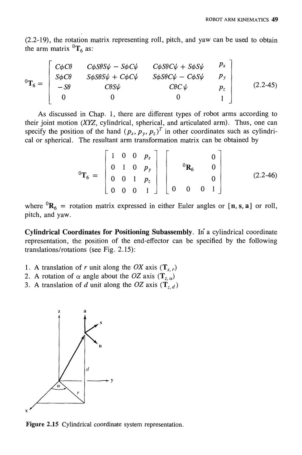
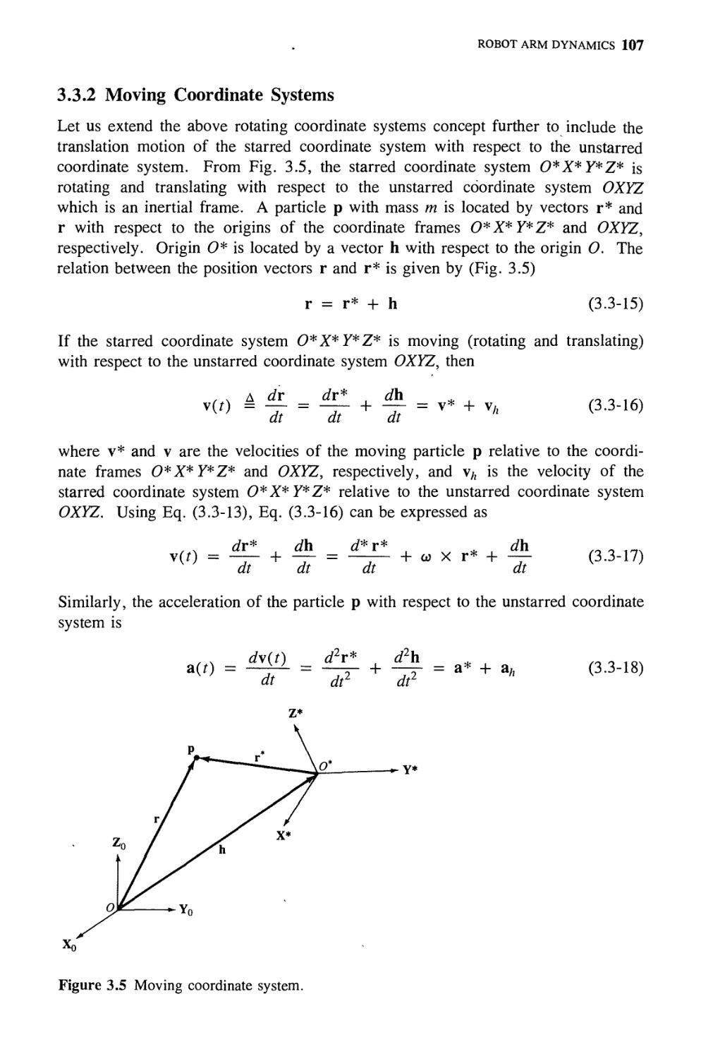
Text
ROBOTICS:
Control, Sensing, Vision, and Intelligence
CAD/CAM, Robotics, and Computer Vision
Consulting Editor
Herbert Freeman, Rutgers University
Fu, Gonzalez, and Lee: Robotics: Control, Sensing, Vision, and Intelligence
Groover, Weiss, Nagel, and Odrey: Industrial Robotics: Technology, Programming,
and Applications
Levine: Vision in Man and Machine
Parsons: Voice and Speech Processing
ROBOTICS:
Control, Sensing, Vision, and Intelligence
K. S. Fu
School of Electrical Engineering
Purdue University
R. C. Gonzalez
Department of Electrical Engineering
University of Tennessee
and
Perceptics Corporation
Knoxville, Tennessee
C. S. G. Lee
School of Electrical Engineering
Purdue University
McGraw-Hill Book Company
New York St. Louis San Francisco Auckland Bogota
Hamburg London Madrid Mexico Milan Montreal New Delhi
Panama Paris Sao Paulo Singapore Sydney Tokyo Toronto
BBbeuft ОшДОВД
Jibwf
TJ
14137
Library of Congress Cataloging-in-Publication Data
Fu, K. S. (King Sun),
Robotics : control, sensing, vision, and intelligence.
(McGraw-Hill series in CAD/CAM robotics and computer
vision)
Bibliography: p.
Includes index.
1. Robotics. I. Gonzalez, Rafael C. II. Lee,
C. S. G. (C. S. George) III. Title.
TJ211.F82 1987 629.8' 92 86-7156
ISBN 0-07-022625-3
ISBN 0-07-022626-1 (solutions manual)
This book was set in Times Roman by House of Equations Inc.
The editor was Sanjeev Rao;
the production supervisor was Diane Renda;
the cover was designed by Laura Stover.
Project supervision was done by Lynn Contrucci.
R. R. Donnelley & Sons Company was printer and binder.
ROBOTICS: CONTROL, SENSING, VISION, AND INTELLIGENCE
Copyright © 1987 by McGraw-Hill, Inc. All rights reserved. Printed in the United States
of America. Except as permitted under the United States Copyright Act of 1976, no part
of this publication may be reproduced or distributed in any form or by any means, or
stored in a data base or retrieval system, without the prior written permission of the
publisher.
234567890 DOCDOC 8 9 8 7
To
Viola,
Connie, and
Pei-Ling
ISBN 0-07-022625-3
ABOUT THE AUTHORS
K. S. Fu was the W. M. Goss Distinguished Professor of Electrical Engineering at
Purdue University. He received his bachelor, master, and Ph.D. degrees from the
National Taiwan University, the University of Toronto, and the University of
Illinois, respectively. Professor Fu was internationally recognized in the engineering
disciplines of pattern recognition, image processing, and artificial intelligence. He
made milestone contributions in both basic and applied research. Often termed the
"father of automatic pattern recognition," Dr. Fu authored four books and more
than 400 scholarly papers. He taught and inspired 75 Ph.D.s. Among his many
honors, he was elected a member of the National Academy of Engineering in 1976,
received the Senior Research Award of the American Society for Engineering
Education in 1981, and was awarded the IEEE's Education Medal in 1982. He was a
Fellow of the IEEE, a 1971 Guggenheim Fellow, and a member of Sigma Xi, Eta
Kappa Nu, and Tau Beta Pi honorary societies. He was the founding president of
the International Association for Pattern Recognition, the founding editor in chief of
the IEEE Transactions of Pattern Analysis and Machine Intelligence, and the editor
in chief or editor for seven leading scholarly journals. Professor Fu died of a heart
attack on April 29, 1985 in Washington, D.C.
R. C. Gonzalez is IBM Professor of Electrical Engineering at the University of
Tennessee, Knoxville, and founder and president of Perceptics Corporation, a high-
technology firm that specializes in image processing, pattern recognition, computer
vision, and machine intelligence. He received his B.S. degree from the University
of Miami, and his M.E. and Ph.D. degrees from the University of Florida,
Gainesville, all in electrical engineering. Dr. Gonzalez is internationally known in his
field, having authored or coauthored over 100 articles and 4 books dealing with
image processing, pattern recognition, and computer vision. He received the 1978
UTK Chancellor's Research Scholar Award, the 1980 Magnavox Engineering
Professor Award, and the 1980 M.E. Brooks Distinguished Professor Award for his
work in these fields. In 1984 he was named Alumni Distinguished Service Professor
ν
VI ABOUT THE AUTHORS
at the University of Tennessee. In 1985 he was named a distinguished alumnus by
the University of Miami. Dr. Gonzalez is a frequent consultant to industry and
government and is a member of numerous engineering professional and honorary
societies, including Tau Beta Pi, Phi Kappa Phi, Eta Kappa Nu, and Sigma Xi. He
is a Fellow of the IEEE.
C. S. G. Lee is an associate professor of Electrical Engineering at Purdue
University. He received his B.S.E.E. and M.S.E.E. degrees from Washington State
University, and a Ph.D. degree from Purdue in 1978. From 1978 to 1985, he was
a faculty member at Purdue and the University of Michigan, Ann Arbor. Dr. Lee
has authored or coauthored more than 40 technical papers and taught robotics short
courses at various conferences. His current interests include robotics and
automation, and computer-integrated manufacturing systems. Dr. Lee has been doing
extensive consulting work for automotive and aerospace industries in robotics. He is
a Distinguished Visitor of the IEEE Computer Society's Distinguished Visitor
Program since 1983, a technical area editor of the IEEE Journal of Robotics and
Automation, and a member of technical committees for various robotics conferences. He
is a coeditor of Tutorial on Robotics, 2nd edition, published by the IEEE Computer
Society Press and a member of Sigma Xi, Tau Beta Pi, the IEEE, and the SME/RI.
CONTENTS
Preface χΐ
1. Introduction
-- У> 1.1. Background
-fe? 1.2. Historical Development
1.3. Robot Arm Kinematics and Dynamics
1.4. Manipulator Trajectory Planning
and Motion Control
1.5. Robot Sensing
~У? 1.6. Robot Programming Languages
1.7. Machine Intelligence
1.8. References
2. Robot Arm Kinematics
2.1. Introduction
2.2. The Direct Kinematics, Problem
2.3. The Inverse Kinematics Solution
2.4. Concluding Remarks
References
Problems
3. Robot Arm Dynamics
3.1. Introduction
3.2. Lagrange-Euler Formulation
3.3. Newton-Euler Formation
3.4. Generalized D'Alembert
Equations of Motion
3,5. Concluding Remarks
References
Problems
1
1
4
6
7
8
9
10
10
12
12
13
52
75
76
76
82
82
84
103
124
142
142
144
VII
viii contents
4· Planning of Manipulator Trajectories 149
4.1. Introduction 149
4.2. General Considerations on
Trajectory Planning 151
4.3. Joint-interpolated Trajectories 154
4.4. Planning of Manipulator Cartesian
Path Trajectories 175
4.5. Concluding Remarks 196
References 197
Problems 198
5. Control of Robot Manipulators 201
5.1. Introduction 201
5.2. Control of the Puma
Robot Arm 203
5.3. Computed Torque Technique 205
5.4. Near-Minimum-Time Control 223
5.5. Variable Structure Control 226
5.6. Nonlinear Decoupled Feedback
Control 227
5.7 Resolved Motion Control 232
5.8. Adaptive Control 244
5.9. Concluding Remarks 263
References 265
Problems 265
6. Sensing 267
267
268
276
284
289
293
293
293
296
296
297
304
307
328
331
359
360
360
6.1.
6.2.
6.3.
6.4.
6.5.
6.6.
Lo>
7.1.
7.2.
7.3.
7.4.
7.5.
7.6.
7.7.
Introduction
Range Sensing
Proximity Sensing
Touch Sensors
Force and Torque Sensing
Concluding Remarks
References
Problems
/V-Level Vision
Introduction
Image Acquisition
Illumination Techniques
Imaging Geometry
Some Basic Relationships Between Pixels
Preprocessing
Concluding Remarks
References
Problems
CONTENTS IX
Higher-Level Vision
8.1. Introduction
8.2. Segmentation
8.3. Description
8.4. Segmentation and Description of
Three-Dimensional Structures
8.5. Recognition
8.6. Interpretation
8.7. Concluding Remarks
References
Problems
Robot Programming Languages
9.1. Introduction
9.2. Characteristics of Robot-
Level Languages
9.3. Characteristics of Task-
Level Languages
9.4. Concluding Remarks
References
Problems
Robot Intelligence and Task Planning
10.1. Introduction
10.2. State Space Search
10.3. Problem Reduction
10.4. Use of Predicate Logic
10.5. Means-Ends Analysis
10.6. Problem-Solving
10.7. Robot Learning
10.8. Robot Task Planning '
10.9. Basic Problems in Task Planning
10.10. Expert Systems and
Knowledge Engineering
10.11. Concluding Remarks
References
362
362
363
395
416
424
439
445
445
447
450
450
451
462
470
472
473
474
474
474
484
489
493
497
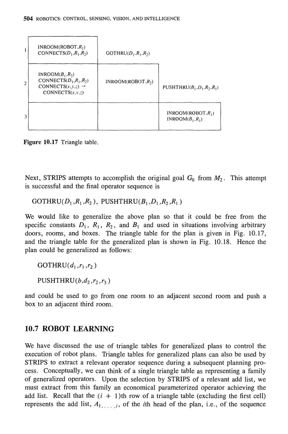
504
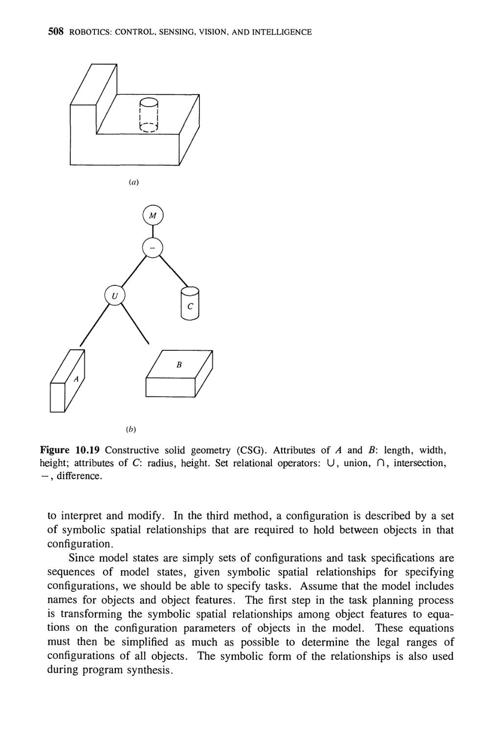
506
509
516
519
520
Appendix 522
A Vectors and Matrices 522
В Manipulator Jacobian 544
Bibliography
Index
556
571
PREFACE
This textbook was written to provide engineers, scientists, and students involved
in robotics and automation with a comprehensive, well-organized, and up-to-
date account of the basic principles underlying the design, analysis, and
synthesis of robotic systems.
The study and development of robot mechanisms can be traced to the
mid-1940s when master-slave manipulators were designed and fabricated at the
Oak Ridge and Argonne National Laboratories for handling radioactive
materials. The first commercial computer-controlled robot was introduced in the late
1950s by Unimation, Inc., and a number of industrial and experimental devices
followed suit during the next 15 years. In spite of the availability of this
technology, however, widespread interest in robotics as a formal discipline of study
and research is rather recent, being motivated by a significant lag in
productivity in most nations of the industrial world.
Robotics is an interdisciplinary field that ranges in scope from the design of
mechanical and electrical components to sensor technology, computer systems,
and artificial intelligence. The bulk of material dealing with robot theory,
design, and applications has been widely scattered in numerous technical
journals, conference proceedings, research monographs, and some textbooks that
either focus attention on some specialized area of robotics or give a "broad-
brush" look of this field. Consequently, it is a rather difficult task, particularly
for a newcomer, to learn the range of principles underlying this subject matter.
This text attempts to put between the covers of one book the basic analytical
techniques and fundamental principles of robotics, and to organize them in a
unified and coherent manner. Thus, the present volume is intended to be of use
both as a textbook and as a reference work. To the student, it presents in a
logical manner a discussion of basic theoretical concepts and important techniques.
For the practicing engineer or scientist, it provides a ready source of reference
in systematic form.
xi
Xll PREFACE
The mathematical level in all chapters is well within the grasp of seniors and
first-year graduate students in a technical discipline such as engineering and
computer science, which require introductory preparation in matrix theory, probability,
computer programming, and mathematical analysis. In presenting the material,
emphasis is placed on the development of fundamental results from basic concepts.
Numerous examples are worked out in the text to illustrate the discussion, and
exercises of various types and complexity are included at the end of each chapter. Some
of these problems allow the reader to gain further insight into the points discussed
in the text through practice in problem solution. Others serve as supplements and
extensions of the material in the book. For the instructor, a complete solutions
manual is available from the publisher.
This book is the outgrowth of lecture notes for courses taught by the authors at
Purdue University, the University of Tennessee, and the University of Michigan.
The material has been tested extensively in the classroom as well as through
numerous short courses presented by all three authors over a 5-year period. The
suggestions and criticisms of students in these courses had a significant influence in
the way the material is presented in this book.
We are indebted to a number of individuals who, directly or indirectly, assisted
in the preparation of the text. In particular, we wish to extend our appreciation to
Professors W. L. Green, G. N. Saridis, R. B. Kelley, J. Y. S. Luh, N. K. Loh, W.
T. Snyder, D. Brzakovic, E. G. Burdette, M. J. Chung, B. H. Lee, and to Dr. R. E.
Woods, Dr. Spivey Douglass, Dr. A. K. Bejczy, Dr. C. Day, Dr. F. King, and Dr.
L-W. Tsai. As is true with most projects carried out in a university environment,
our students over the past few years have influenced not only our thinking, but also
the topics covered in this book. The following individuals have worked with us in
the course of their advanced undergraduate or graduate programs: J. A. Herrera,
M. A. Abidi, R. O. Eason, R. Safabakhsh, A. P. Perez, C. H. Hayden, D. R.
Cate, K. A. Rinehart, N. Alvertos, E. R. Meyer, P. R. Chang, C. L. Chen, S. H.
Hou, G. H. Lee, R. Jungclas, Huarg, and D. Huang. Thanks are also due to Ms.
Susan Merrell, Ms. Denise Smiddy, Ms. Mary Bearden, Ms. Frances Bourdas, and
Ms. Mary Ann Pruder for typing numerous versions of the manuscript. In addition,
we express our appreciation to the National Science Foundation, the Air Force
Office of Scientific Research, the Office of Naval Research, the Army Research
Office, Westinghouse, Martin Marietta Aerospace, Martin Marietta Energy Systems,
Union Carbide, Lockheed Missiles and Space Co., The Oak Ridge National
Laboratory, and the University of Tennessee Measurement and Control Center for their
sponsorship of our research activities in robotics, computer vision, machine
intelligence, and related areas.
K. S. Fu
R. C. Gonzalez
С S. G. Lee
PREFACE Xlll
Professor King-Sun Fu died of a heart attack on April 29, 1985, in
Washington, D.C., shortly after completing his contributions to this book. He
will be missed by all those who were fortunate to know him and to work with
him during a productive and distinguished career.
R. С G.
C. S. G. L.
CHAPTER
ONE
INTRODUCTION
One machine can do the work of a
hundred ordinary men, but no machine
can do the work of one extraordinary man.
Elbert Hubbard
1.1 BACKGROUND
With a pressing need for increased productivity and the delivery of end products of
uniform quality, industry is turning more and more toward computer-based
automation. At the present time, most automated manufacturing tasks are carried out
by special-purpose machines designed to perform predetermined functions in a
manufacturing process. The inflexibility and generally high cost of these
machines, often called hard automation systems, have led to a broad-based interest
in the use of robots capable of performing a variety of manufacturing functions in
a more flexible working environment and at lower production costs.
The word robot originated from the Czech word robota, meaning work.
Webster's dictionary defines robot as "an automatic device that performs functions
ordinarily ascribed to human beings." With this definition, washing machines may
be considered robots. A definition used by the Robot Institute of America gives a
more precise description of industrial robots: "A robot is a reprogrammable
multi-functional manipulator designed to move materials, parts, tools, or
specialized devices, through variable programmed motions for the performance of a
variety of tasks." In short, a robot is a reprogrammable general-purpose
manipulator with external sensors that can perform various assembly tasks. With this
definition, a robot must possess intelligence, which is normally due to computer
algorithms associated with its control and sensing systems.
An industrial robot is a general-purpose, computer-controlled manipulator
consisting of several rigid links connected in series by revolute or prismatic joints.
One end of the chain is attached to a supporting base, while the other end is free
and equipped with a tool to manipulate objects or perform assembly tasks. The
motion of the joints results in relative motion of the links. Mechanically, a robot
is composed of an arm (or mainframe) and a wrist subassembly plus a tool. It is
designed to reach a workpiece located within its work volume. The work volume
is the sphere of influence of a robot whose arm can deliver the wrist subassembly
unit to any point within the sphere. The arm subassembly generally can move
with three degrees of freedom. The combination of the movements positions the
1
2 ROBOTICS: CONTROL, SENSING, VISION, AND INTELLIGENCE
wrist unit at the workpiece. The wrist subassembly unit usually consists of three
rotary motions. The combination of these motions orients the tool according to the
configuration of the object for ease in pickup. These last three motions are often
called pitch, yaw, and roll. Hence, for a six-jointed robot, the arm subassembly is
the positioning mechanism, while the wrist subassembly is the orientation
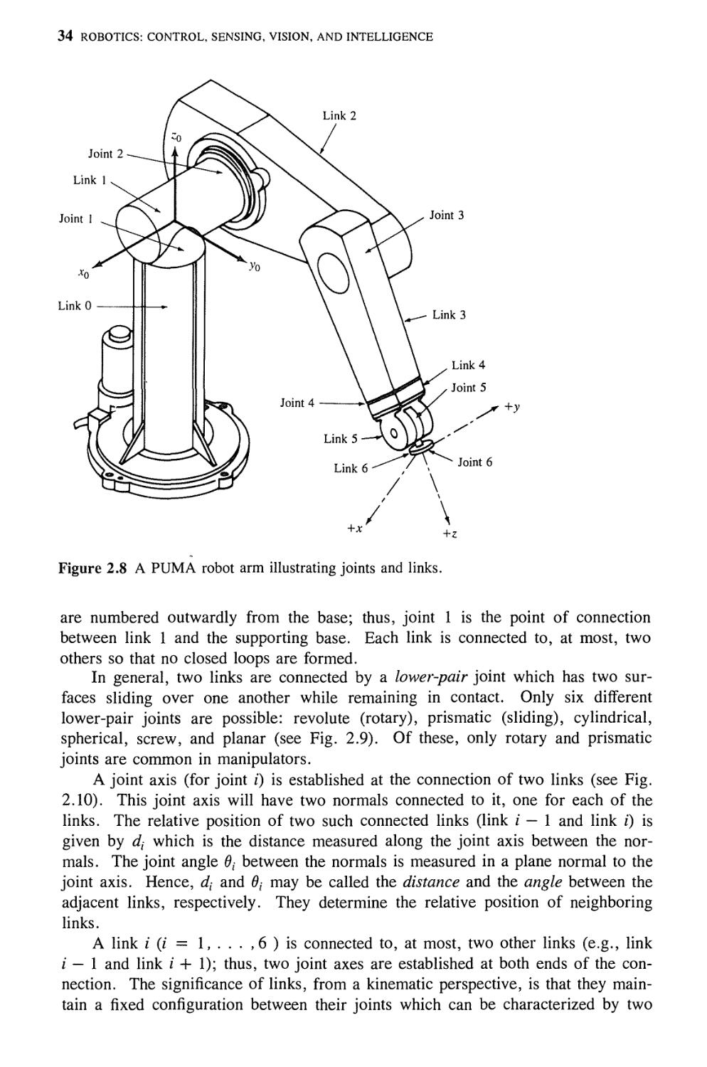
mechanism. These concepts are illustrated by the Cincinnati Milacron Γ3 robot and the
Unimation PUMA robot arm shown in Fig. 1.1.
Roll
Base
Waist rotation 320°
Shoulder rotation 300°
Elbow rotation 270°
30.0 in
Wrist bend 200°
Flange
rotation 270°
Φ)
Gripper mounting
& \^ Wrist rotation 300°
Figure 1.1 (a) Cincinnati Milacron T3 robot arm. (b) PUMA 560 series robot arm.
INTRODUCTION 3
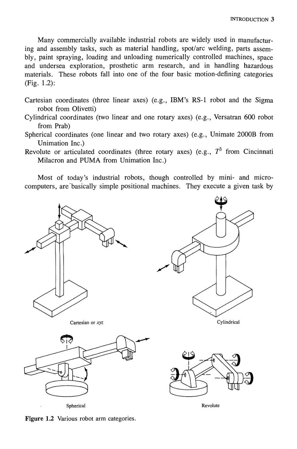
Many commercially available industrial robots are widely used in
manufacturing and assembly tasks, such as material handling, spot/arc welding, parts
assembly, paint spraying, loading and unloading numerically controlled machines, space
and undersea exploration, prosthetic arm research, and in handling hazardous
materials. These robots fall into one of the four basic motion-defining categories
(Fig. 1.2):
Cartesian coordinates (three linear axes) (e.g., IBM's RS-1 robot and the Sigma
robot from Olivetti)
Cylindrical coordinates (two linear and one rotary axes) (e.g., Versatran 600 robot
from Prab)
Spherical coordinates (one linear and two rotary axes) (e.g., Unimate 2000B from
Unimation Inc.)
Revolute or articulated coordinates (three rotary axes) (e.g., T3 from Cincinnati
Milacron and PUMA from Unimation Inc.)
Most of today's industrial robots, though controlled by mini- and
microcomputers, are basically simple positional machines. They execute a given task by
Spherical Revolute
Figure 1.2 Various robot arm categories.
4 ROBOTICS: CONTROL, SENSING, VISION, AND INTELLIGENCE
playing back prerecorded or preprogrammed sequences of motions that have been
previously guided or taught by a user with a hand-held control-teach box.
Moreover, these robots are equipped with little or no external sensors for obtaining the
information vital to its working environment. As a result, robots are used mainly
in relatively simple, repetitive tasks. More research effort is being directed toward
improving the overall performance of the manipulator systems, and one way is
through the study of the various important areas covered in this book.
1.2 HISTORICAL DEVELOPMENT
The word robot was introduced into the English language in 1921 by the
playwright Karel Capek in his satirical drama, R.U.R. (Rossum's Universal Robots).
In this work, robots are machines that resemble people, but work tirelessly.
Initially, the robots were manufactured for profit to replace human workers but,
toward the end, the robots turned against their creators, annihilating the entire
human race. Capek's play is largely responsible for some of the views popularly
held about robots to this day, including the perception of robots as humanlike
machines endowed with intelligence and individual personalities. This image was
reinforced by the 1926 German robot film Metropolis, by the walking robot
Electro and his dog Spar ко, displayed in 1939 at the New York World's Fair, and more
recently by the robot C3PO featured in the 1977 film Star Wars, Modern
industrial robots certainly appear primitive when compared with the expectations created
by the communications media during the past six decades.
Early work leading to today's industrial robots can be traced to the period
immediately following World War II. During the late 1940s research programs
were started at the Oak Ridge and Argonne National Laboratories to develop
remotely controlled mechanical manipulators for handling radioactive materials.
These systems were of the "master-slave" type, designed to reproduce faithfully
hand and arm motions made by a human operator. The master manipulator was
guided by the user through a sequence of motions, while the slave manipulator
duplicated the master unit as closely as possible. Later, force feedback was added
by mechanically coupling the motion of the master and slave units so that the
operator could feel the forces as they developed between the slave manipulator and
its environment. In the mid-1950s the mechanical coupling was replaced by
electric and hydraulic power in manipulators such as General Electric's Handyman and
the Minotaur I built by General Mills.
The work on master-slave manipulators was quickly followed by more
sophisticated systems capable of autonomous, repetitive operations. In the mid-1950s
George C. Devol developed a device he called a "programmed articulated transfer
device," a manipulator whose operation could be programmed (and thus changed)
and which could follow a sequence of motion steps determined by the instructions
in the program. Further development of this concept by Devol and Joseph F.
Engelberger led to the first industrial robot, introduced by Unimation Inc. in 1959.
The key to this device was the use of a computer in conjunction with a manipula-
INTRODUCTION 5
tor to produce a machine that could be "taught" to carry out a variety of tasks
automatically. Unlike hard automation machines, these robots could be repro-
grammed and retooled at relative low cost to perform other jobs as manufacturing
requirements changed.
While programmed robots offered a novel and powerful manufacturing tool, it
became evident in the 1960s that the flexibility of these machines could be
enhanced significantly by the use of sensory feedback. Early in that decade, H. A.
Ernst [1962] reported the development of a computer-controlled mechanical hand
with tactile sensors. This device, called the MH-1, could "feel" blocks and use
this information to control the hand so that it stacked the blocks without operator
assistance. This work is one of the first examples of a robot capable of adaptive
behavior in a reasonably unstructured environment. The manipulative system
consisted of an ANL Model-8 manipulator with 6 degrees of freedom controlled by a
TX-0 computer through an interfacing device. This research program later
evolved as part of project MAC, and a television camera was added to the
manipulator to begin machine perception research. During the same period, Tomovic and
Boni [1962] developed a prototype hand equipped with a pressure sensor which
sensed the object and supplied an input feedback signal to a motor to initiate one
of two grasp patterns. Once the hand was in contact with the object, information
proportional to object size and weight was sent to a computer by these pressure-
sensitive elements. In 1963, the American Machine and Foundry Company (AMF)
introduced the VERSATRAN commercial robot. Starting in this same year,
various arm designs for manipulators were developed, such as the Roehampton arm
and the Edinburgh arm.
In the late 1960s, McCarthy [1968] and his colleagues at the Stanford
Artificial Intelligence Laboratory reported development of a computer with hands,
eyes, and ears (i.e., manipulators, TV cameras, and microphones). They
demonstrated a system that recognized spoken messages, "saw" blocks scattered on a
table, and manipulated them in accordance with instructions. During this period,
Pieper [1968] studied the kinematic problem of a computer-controlled manipulator
while Kahn and Roth [1971] analyzed the dynamics and control of a restricted arm
using bang-bang (near minimum time) control.
Meanwhile, other countries (Japan in particular) began to see the potential of
industrial robots. As early as 1968, the Japanese company Kawasaki Heavy
Industries negotiated a license with Unimation for its robots. One of the more unusual
developments in robots occurred in 1969, when an experimental walking truck was
developed by the General Electric Company for the U.S. Army. In the same year,
the Boston arm was developed, and in the following year the Stanford arm was
developed, which was equipped with a camera and computer controller. Some of
the most serious work in robotics began as these arms were used as robot
manipulators. One experiment with the Stanford arm consisted of automatically stacking
blocks according to various strategies. This was very sophisticated work for an
automated robot at that time. In 1974, Cincinnati Milacron introduced its first
computer-controlled industrial robot. Called "The Tomorrow Tool," or Γ3, it
could lift over 100 lb as well as track moving objects on an assembly line.
6 ROBOTICS: CONTROL, SENSING, VISION, AND INTELLIGENCE
During the 1970s a great deal of research work focused on the use of external
sensors to facilitate manipulative operations. At Stanford, Bolles and Paul [1973],
using both visual and force feedback, demonstrated a computer-controlled Stanford
arm connected to a PDP-10 computer for assembling automotive water pumps. At
about the same time, Will and Grossman [1975] at IBM developed a computer-
controlled manipulator with touch and force sensors to perform mechanical
assembly of a 20-part typewriter. Inoue [1974] at the MIT Artificial Intelligence
Laboratory worked on the artificial intelligence aspects of force feedback. A
landfall navigation search technique was used to perform initial positioning in a
precise assembly task. At the Draper Laboratory Nevins et al. [1974] investigated
sensing techniques based on compliance. This work developed into the
instrumentation of a passive compliance device called remote center compliance (RCC)
which was attached to the mounting plate of the last joint of the manipulator for
close parts-mating assembly. Bejczy [1974], at the Jet Propulsion Laboratory,
implemented a computer-based torque-control technique on his extended Stanford
arm for space exploration projects. Since then, various control methods have been
proposed for servoing mechanical manipulators.
Today, we view robotics as a much broader field of work than we did just a
few years ago, dealing with research and development in a number of
interdisciplinary areas, including kinematics, dynamics, planning systems, control, sensing,
programming languages, and machine intelligence. These topics, introduced
briefly in the following sections, constitute the core of the material in this book.
1.3 ROBOT ARM KINEMATICS AND DYNAMICS
Robot arm kinematics deals with the analytical study of the geometry of motion of
a robot arm with respect to a fixed reference coordinate system without regard to
the forces/moments that cause the motion. Thus, kinematics deals with the
analytical description of the spatial displacement of the robot as a function of time, in
particular the relations between the joint-variable space and the position and
orientation of the end-effector of a robot arm.
There are two fundamental problems in robot arm kinematics. The first
problem is usually referred to as the direct (or forward) kinematics problem, while the
second problem is the inverse kinematics (or arm solution) problem. Since the
independent variables in a robot arm are the joint variables, and a task is usually
stated in terms of the reference coordinate frame, the inverse kinematics problem
is used more frequently. Denavit and Hartenberg [1955] proposed a systematic
and generalized approach of utilizing matrix algebra to describe and represent the
spatial geometry of the links of a robot arm with respect to a fixed reference
frame. This method uses a 4 X 4 homogeneous transformation matrix to describe
the spatial relationship between two adjacent rigid mechanical links and reduces the
direct kinematics problem to finding an equivalent 4x4 homogeneous
transformation matrix that relates the spatial displacement of the hand coordinate frame to the
reference coordinate frame. These homogeneous transformation matrices are also
useful in deriving the dynamic equations of motion of a robot arm. In general, the
INTRODUCTION 7
inverse kinematics problem can be solved by several techniques. The most
commonly used methods are the matrix algebraic, iterative, or geometric approach.
Detailed treatments of direct kinematics and inverse kinematics problems are given
in Chap. 2.
Robot arm dynamics, on the other hand, deals with the mathematical
formulations of the equations of robot arm motion. The dynamic equations of motion of a
manipulator are a set of mathematical equations describing the dynamic behavior
of the manipulator. Such equations of motion are useful for computer simulation
of the robot arm motion, the design of suitable control equations for a robot arm,
and the evaluation of the kinematic design and structure of a robot arm. The
actual dynamic model of an arm can be obtained from known physical laws such
as the laws of newtonian and lagrangian mechanics. This leads to the development
of dynamic equations of motion for the various articulated joints of the manipulator
in terms of specified geometric and inertial parameters of the links. Conventional
approaches like the Lagrange-Euler and the Newton-Euler formulations can then be
applied systematically to develop the actual robot arm motion equations. Detailed
discussions of robot arm dynamics are presented in Chap. 3.
1.4 MANIPULATOR TRAJECTORY PLANNING
AND MOTION CONTROL
With the knowledge of kinematics and dynamics of a serial link manipulator, one
would like to servo the manipulator's joint actuators to accomplish a desired task
by controlling the manipulator to fol ν a desired path. Before moving the robot
arm, it is of interest to know whether there are any obstacles present in the path
that the robot arm has to traverse (obstacle constraint) and whether the manipulator
hand needs to traverse along a specified path (path constraint). The control
problem of a manipulator can be conveniently divided into two coherent
subproblems—the motion (or trajectory) planning subproblem and the motion
control subproblem.
The space curve that the manipulator hand moves along from an initial
location (position and orientation) to the final location is called the path. The trajectory
planning (or trajectory planner) interpolates and/or approximates the desired path
by a class of polynomial functions and generates a sequence of time-based "control
set points" for the control of the manipulator from the initial location to the
destination location. Chapter 4 discusses the various trajectory planning schemes for
obstacle-free motion, as well as the formalism for describing desired manipulator
motion in terms of sequences of points in space through which the manipulator
must pass and the space curve that it traverses.
In general, the motion control problem consists of (1) obtaining dynamic
models of the manipulator, and (2) using these models to determine control laws or
strategies to achieve the desired system response and performance. Since the first
part of the control problem is discussed extensively in Chap. 3, Chap. 5
concentrates on the second part of the control problem. From the control analysis point
of view, the movement of a robot arm is usually performed in two distinct control
8 ROBOTICS: CONTROL, SENSING, VISION, AND INTELLIGENCE
phases. The first is the gross motion control in which the arm moves from an
initial position/orientation to the vicinity of the desired target position/orientation
along a planned trajectory. The second is the fine motion control in which the
end-effector of the arm dynamically interacts with the object using sensory
feedback information from the sensors to complete the task.
Current industrial approaches to robot arm control treat each joint of the robot
arm as a simple joint servomechanism. The servomechanism approach models the
varying dynamics of a manipulator inadequately because it neglects the motion and
configuration of the whole arm mechanism. These changes in the parameters of
the controlled system sometimes are significant enough to render conventional
feedback control strategies ineffective. The result is reduced servo response speed
and damping, limiting the precision and speed of the end-effector and making it
appropriate only for limited-precision tasks. Manipulators controlled in this
manner move at slow speeds with unnecessary vibrations. Any significant
performance gain in this and other areas of robot arm control require the consideration
of more efficient dynamic models, sophisticated control approaches, and the use of
dedicated computer architectures and parallel processing techniques. Chapter 5
focuses on deriving gross motion control laws and strategies which utilize the
dynamic models discussed in Chap. 3 to efficiently control a manipulator.
1.5 ROBOT SENSING
The use of external sensing mechanisms allows a robot to interact with its
environment in a flexible manner. This is in contrast to preprogrammed operations in
which a robot is "taught" to perform repetitive tasks via a set of programmed
functions. Although the latter is by far the most predominant form of operation of
present industrial robots, the use of sensing technology to endow machines with a
greater degree of intelligence in dealing with their environment is indeed an active
topic of research and development in the robotics field.
The function of robot sensors may be divided into two principal categories:
internal state and external state. Internal state sensors deal with the detection of
variables such as arm joint position, which are used for robot control. External
state sensors, on the other hand, deal with the detection of variables such as range,
proximity, and touch. External sensing, the topic of Chaps. 6 through 8, is used
for robot guidance, as well as for object identification and handling. The focus of
Chap. 6 is on range, proximity, touch, and force-torque sensing. Vision sensors
and techniques are discussed in detail in Chaps. 7 and 8. Although proximity,
touch, and force sensing play a significant role in the improvement of robot
performance, vision is recognized as the most powerful of robot sensory capabilities.
Robot vision may be defined as the process of extracting, characterizing, and
interpreting information from images of a three-dimensional world. This process, also
commonly referred to as machine or computer vision, may be subdivided into six
principal areas: (1) sensing, (2) preprocessing, (3) segmentation, (4) description,
(5) recognition, and (6) interpretation.
INTRODUCTION 9
It is convenient to group these various areas of vision according to the
sophistication involved in their implementation. We consider three levels of processing:
low-, medium-, and high-level vision. While there are no clearcut boundaries
between these subdivisions, they do provide a useful framework for categorizing
the various processes that are inherent components of a machine vision system. In
our discussion, we shall treat sensing and preprocessing as low-level vision
functions. This will take us from the image formation process itself to compensations
such as noise reduction, and finally to the extraction of primitive image features
such as intensity discontinuities. We will associate with medium-level vision those
processes that extract, characterize, and label components in an image resulting
from low-level vision. In terms of our six subdivisions, we will treat
segmentation, description, and recognition of individual objects as medium-level vision
functions. High-level vision refers to processes that attempt to emulate cognition.
The material in Chap. 7 deals with sensing, preprocessing, and with concepts and
techniques required to implement low-level vision functions. Topics in higher-level
vision are discussed in Chap. 8.
1.6 ROBOT PROGRAMMING LANGUAGES
One major obstacle in using manipulators as general-purpose assembly machines is
the lack of suitable and efficient communication between the user and the robotic
system so that the user can direct the manipulator to accomplish a given task.
There are several ways to communicate with a robot, and the three major
approaches to achieve it are discrete word recognition, teach and playback, and
high-level programming languages.
Current state-of-the-art speech recognition is quite primitive and generally
speaker-dependent. It can recognize a set of discrete words from a limited
vocabulary and usually requires the user to pause between words. Although it is now
possible to recognize words in real time due to faster computer components and
efficient processing algorithms, the usefulness of discrete word recognition to
describe a task is limited. Moreover, it requires a large memory space to store
speech data, and it usually requires a training period to build up speech templates
for recognition.
The method of teach and playback involves teaching the robot by leading it
through the motions to be performed. This is usually accomplished in the
following steps: (1) leading the robot in slow motion using manual control through the
entire assembly task, with the joint angles of the robot at appropriate locations
being recorded in order to replay the motion; (2) editing and playing back the
taught motion; and (3) if the taught motion is correct, then the robot is run at an
appropriate speed in a repetitive motion. This method is also known as guiding
and is the most commonly used approach in present-day industrial robots.
A more general approach to solve the human-robot communication problem is
the use of high-level programming. Robots are commonly used in areas such as
arc welding, spot welding, and paint spraying. These tasks require no interaction
10 ROBOTICS: CONTROL, SENSING, VISION, AND INTELLIGENCE
between the robot and the environment and can be easily programmed by guiding.
However, the use of robots to perform assembly tasks generally requires high-level
programming techniques. This effort is warranted because the manipulator is
usually controlled by a computer, and the most effective way for humans to
communicate with computers is through a high-level programming language. Furthermore,
using programs to describe assembly tasks allows a robot to perform different jobs
by simply executing the appropriate program. This increases the flexibility and
versatility of the robot. Chapter 9 discusses the use of high-level programming
techniques for achieving effective communication with a robotic system.
L7 ROBOT INTELLIGENCE
A basic problem in robotics is planning motions to solve some prespecified task,
and then controlling the robot as it executes the commands necessary to achieve
those actions. Here, planning means deciding on a course of action before acting.
This action synthesis part of the robot problem can be solved by a problem-solving
system that will achieve some stated goal, given some initial situation. A plan is,
thus, a representation of a course of action for achieving a stated goal.
Research on robot problem solving has led to many ideas about problem-
solving systems in artificial intelligence. In a typical formulation of a robot
problem we have a robot that is equipped with sensors and a set of primitive actions
that it can perform in some easy-to-understand world. Robot actions change one
state, or configuration, of the world into another. In the "blocks world," for
example, we imagine a world of several labeled blocks resting on a table or on
each other and a robot consisting of a TV camera and a movable arm and hand
that is able to pick up and move blocks. In some situations, the robot is a mobile
vehicle with a TV camera that performs tasks such as pushing objects from place
to place in an environment containing other objects.
In Chap. 10, we introduce several basic methods for problem solving and their
applications to robot planning. The discussion emphasizes the problem-solving or
planning aspect of a robot. A robot planner attempts to find a path from our
initial robot world to a final robot world. The path consists of a sequence of
operations that are considered primitive to the system. A solution to a problem could
be the basis of a corresponding sequence of physical actions in the physical world.
Rot^ot planning, which provides the intelligence and problem-solving capability to
a robot system, is still a very active area of research. For real-time robot
applications, we still need powerful and efficient planning algorithms that will be executed
by high-speed special-purpose computer systems.
1·8 REFERENCES
The general references cited below are representative of publications dealing with
topics of interest in robotics and related fields. References given at the end of
INTRODUCTION 11
later chapters are keyed to specific topics discussed in the text. The bibliography
at the end of the book is organized in alphabetical order by author, and it contains
all the pertinent information for each reference cited in the text.
Some of the major journals and conference proceedings that routinely contain
articles on various aspects of robotics include: IEEE Journal of Robotics and
Automation', International Journal of Robotics Research] Journal of Robotic Systems;
Robotica\ IEEE Transactions on Systems, Man and Cybernetics; Artificial
Intelligence; IEEE Transactions on Pattern Analysis and Machine Intelligence; Computer
Graphics, Vision, and Image Processing; Proceedings of the International
Symposium on Industrial Robots; Proceedings of the International Joint Conference on
Artificial Intelligence; Proceedings of IEEE International Conference on Robotics
and Automation; IEEE Transactions on Automatic Control; Mechanism and
Machine Theory; Proceedings of the Society of Photo-Optical and Instrumentation
Engineers; ASME Journal of Mechanical Design; ASME Journal of Applied
Mechanics; ASME Journal of Dynamic Systems, Measurement and Control; and
ASME Journal of Mechanisms, Transmissions, and Automation in Design.
Complementary reading for the material in this book may be found in the
books by Dodd and Rossol [1979], Engelberger [1980], Paul [1981], Dorf [1983],
Snyder [1985], Lee, Gonzalez, and Fu [1986], Tou [1985], and Craig [1986].
\
CHAPTER
TWO
ROBOT ARM KINEMATICS
And see! she stirs, she starts,
she moves, she seems to feel
the thrill of life!
Henry Wadsworth Longfellow
4
2.1 INTRODUCTION
A mechanical manipulator can be modeled as an open-loop articulated chain with
several rigid bodies (links) connected in series by either revolute or prismatic
joints driven by actuators. One end of the chain is attached to a supporting base
while the other end is free and attached with a tool (the end-effector) to manipulate
objects or perform assembly tasks. The relative motion of the joints results in the
motion of the links that positions the hand in a desired orientation. In most
robotic applications, one is interested in the spatial description of the end-effector
of the manipulator with respect to a fixed reference coordinate system.
Robot arm kinematics deals with the analytical study of the geometry of
motion of a robot arm with respect to a fixed reference coordinate system as a
function of time without regard to the forces/moments that cause the motion.
Thus, it deals with the analytical description of the spatial displacement of the
robot as a function of time, in particular the relations between the joint-variable
space and the position and orientation of the end-effector of a robot arm. This
chapter addresses two fundamental questions of both theoretical and practical
interest in robot arm kinematics:
1. For a given manipulator, given the joint angle vector q(t) = (q\(t),
4i(t) > · · · >Яп(0)Т anc* the geometric link parameters, where η is the number
of degrees of freedom, what is the position and orientation of the end-effector
of the manipulator with respect to a reference coordinate system?
2. Given a desired position and orientation of the end-effector of the manipulator
and the geometric link parameters with respect to a reference coordinate
system, can the manipulator reach the desired prescribed manipulator hand position
and orientation? And if it can, how many different manipulator configurations
will satisfy the same condition?
The first question is usually referred to as the direct (or forward) kinematics
problem, while the second question is the inverse kinematics (or arm solution) problem.
12
ROBOT ARM KINEMATICS 13
Link parameters
in
Joint
angles
Joint
angles -«.
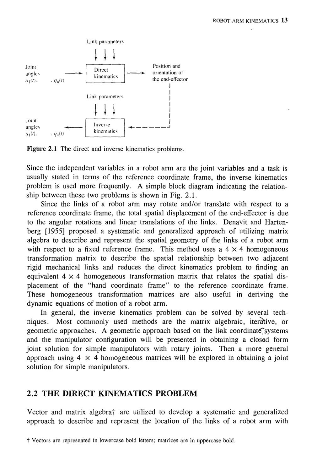
Figure 2.1 The direct and inverse kinematics problems.
Since the independent variables in a robot arm are the joint variables and a task is
usually stated in terms of the reference coordinate frame, the inverse kinematics
problem is used more frequently. A simple block diagram indicating the
relationship between these two problems is shown in Fig. 2.1.
Since the links of a robot arm may rotate and/or translate with respect to a
reference coordinate frame, the total spatial displacement of the end-effector is due
to the angular rotations and linear translations of the links. Denavit and Harten-
berg [1955] proposed a systematic and generalized approach of utilizing matrix
algebra to describe and represent the spatial geometry of the links of a robot arm
with respect to a fixed reference frame. This method uses a 4 X 4 homogeneous
transformation matrix to describe the spatial relationship between two adjacent
rigid mechanical links and reduces the direct kinematics problem to finding an
equivalent 4x4 homogeneous transformation matrix that relates the spatial
displacement of the "hand coordinate frame" to the reference coordinate frame.
These homogeneous transformation matrices are also useful in deriving the
dynamic equations of motion of a robot arm.
In general, the inverse kinematics problem can be solved by several
techniques. Most commonly used methods are the matrix algebraic, iterative, or
geometric approaches. A geometric approach based on the link coordinat67sy stems
and the manipulator configuration will be presented in obtaining a closed form
joint solution for simple manipulators with rotary joints. Then a more general
approach using 4x4 homogeneous matrices will be explored in obtaining a joint
solution for simple manipulators.
2.2 THE DIRECT KINEMATICS PROBLEM
Vector and matrix algebraf are utilized to develop a systematic and generalized
approach to describe and represent the location of the links of a robot arm with
t Vectors are represented in lowercase bold letters; matrices are in uppercase bold.
Direct
kinematics
Link parameters
I II
Inverse
kinematics
Position and
orientation of
the end-effect or
I
I
14 ROBOTICS' CONTROL, SENSING. VISION. AND INTELLIGENCE
respect to a fixed reference frame. Since the links of a robot arm may rotate and/
or translate with respect to a reference coordinate frame, a body-attached
coordinate frame will be established along the joint axis for each link. The direct
kinematics problem is reduced to finding a transformation matrix that relates the
body-attached coordinate frame to the reference coordinate frame. A 3 χ 3
rotation matrix is used to describe the rotational operations of the body-attached frame
with respect to the reference frame. The homogeneous coordinates are then used
to represent position vectors in a three-dimensional space, and the rotation matrices
will be expanded to 4 χ 4 homogeneous transformation matrices to include the
translational operations of the body-attached coordinate frames. This matrix
representation of a rigid mechanical link to describe the spatial geometry of a
robot'arm was first used by Denavit and Hartenberg [1955J. The advantage of
using- the Denavit-Hartenberg representation of linkages is its algorithmic
universality in deriving the kinematic equation of a robot arm.
2.2.1 Rotation Matrices
A 3 χ 3 rotation matrix can be defined as a transformation matrix which operates
on a position vector in a three-dimensional euclidean space and maps its
coordinates expressed in a rotated coordinate system OUVW (body-attached frame) to a
reference coordinate system OXYZ. In Fig. 2.2, we are given two right-hand
rectangular coordinate systems, namely, the OXYZ coordinate system with OX, OY,
and OZ as its coordinate axes and the OUVW coordinate system with OU, OV, and
OW as its coordinate axes. Both coordinate systems have their origins coincident at
point O. The OXYZ coordinate system is fixed in the three-dimensional space and
is considered to be the reference frame. The OUVW coordinate frame is rotating
with respect to the reference frame OXYZ. Physically,' one can consider the
OUVW coordinate system to be a body-attached coordinate frame. That is, it is
ζ
ρ
1— j;»
/ Τ W У^
χ
Figure 2.2 Reference and body-attached coordinate systems.
ROBOT ARM KINEMATICS 15
permanently and conveniently attached to the rigid body (e.g., an aircraft or a link
of a robot arm) and moves together with it. Let (iv, jy, kz) and (iM, jv, kw) be
the unit vectors along the coordinate axes of the OXYZ and OUVW systems,
respectively. A point ρ in the space can be represented by its coordinates with
respect to both coordinate systems. For ease of discussion, we shall assume that ρ
is at rest and fixed with respect to the OUVW coordinate frame. Then the point ρ
can be represented by its coordinates with respect to the OUVW and OXYZ
coordinate systems, respectively, as
Vuvw = (Pu> Pv> Pwf and pxyz = (px, py, pz)T (2.2-1)
where pxyz and puvw represent the same point ρ in the space with reference to
different coordinate systems, and the superscript Τ on vectors and matrices denotes
the transpose operation.
We would like to find a 3 X 3 transformation matrix R that will transform the
coordinates of puvw to the coordinates expressed with respect to the OXYZ
coordinate system, after the OUVW coordinate system has been rotated. That is,
Pxyz = RP«mv (2·2"2)
Note that physically the point pMVW has been rotated together with the OUVW
coordinate system.
Recalling the definition of the components of a vector, we have
Puvw = PiX< + PvL + PwK (2.2-3)
where px, py, and pz represent the components of ρ along the OX, OY, and OZ
axes, respectively, or the projections of ρ onto the respective axes. Thus, using
the definition of a scalar product and Eq. (2.2-3),
Px - h 'P = Ух -КРи + \χ *ivPv + iv 'KPw
Pv = j>. *P = j>> *KPu + Jv *JvPv + Jv mKPw (2.2-4)
P:: = Κ ·Ρ = Κ ·ί«Ρ« + Κ mivPv + К *KPw
or expressed in matrix form,
Px
Py
Pz
=
J ν · К
к- · К
Pu
Pv
Pw
(2.2-5)
16 ROBOTICS: CONTROL, SENSING, VISION, AND INTELLIGENCE
Using this notation, the matrix R in Eq. (2.2-2) is given by
R =
\x " ht
J у *м
К ' i«
ix #Jv
Jy *Jv
К ' Jv
\x ' К
iy · К
К · kw
(2.2-6)
Similarly, one can obtain the coordinates of puvw from the coordinates of pxyz:
VuVW = QVxyz (2.2-7)
^or
- -
Pu
Pv
Pw
—
-
i« ' l
Jv ' ix
к -i
"Vv lx
К 'jy
Jv *Jy
К 'jy
К ' ^
Jv ' К
К · кг
-
Λ·
Py
pz
(2.2-8)
Since dot products are commutative, one can see from Eqs. (2.2-6) to (2.2-8)
that
and
Q = R-l = R^
QR = RrR = R-'R = I3
(2.2-9)
(2.2-10)
where I3 is a 3 X 3 identity matrix. The transformation given in Eq. (2.2-2) or
(2.2-7) is called an orthogonal transformation and since the vectors in the dot
products are all unit vectors, it is also called an orthonormal transformation.
The primary interest in developing the above transformation matrix is to find
the rotation matrices that represent rotations of the OUVW coordinate system about
each of the three principal axes of the reference coordinate system OXYZ. If the
OUVW coordinate system is rotated an a angle about the OX axis to arrive at a
new location in the space, then the point pimv having coordinates (pu, pv> pw)T
with respect to the OUVW system will have different coordinates (px, py> pz)T
with respect to the reference system OXYZ. The necessary transformation matrix
Rxa is called the rotation matrix about the OX axis with a angle. Rxa can be
derived from the above transformation matrix concept, that is
Pxyz **x,a Puvw
(2.2-11)
with L =
Rr.a —
and
lr ·!
h 'Jv
Jy 'Jv
К "Jv
iy -K
К · kw
1 0 0
0 cos α — sin α
0 sin a cos a
(2.2-12)
Similarly, the 3 X 3 rotation matrices for rotation about the OY axis with φ angle
and about the OZ axis with θ angle are, respectively (see Fig. 2.3),
ROBOT ARM KINEMATICS 17
! Ik
+*Y
a= 90°
- У
w L
/
+ Y
и
X 0-90° X
Figure 2.3 Rotating coordinate systems.
*Y
18 ROBOTICS: CONTROL, SENSING, VISION, AND INTELLIGENCE
Rv
cos φ 0 sin φ
0 1 0
— sin φ 0 cos φ
R? я —
cos0 -sin0 Ο
sin θ cos θ Ο
0 0 1
(2.2-13)
The matrices RXi(X, R^, and RZ)d are called the basic rotation matrices. Other
finite rotation matrices can be obtained from these matrices.
Example: Given two points aMvnv = (4, 3, 2)T and buvw = (6, 2, 4)T with
respect to the rotated OUVW coordinate system, determine the corresponding
points 2ixyzy hxyz with respect to the reference coordinate system if it has been
rotated 60° about the OZ axis.
"xyz
Solution: axvz = R^o" a«vw and
0.500 -0.866 0
0.866 0.500 0
0 0 1
bxyz — R:
4
3
2
Z,60° "uvw
Ч*;уг
4(0.5) + 3(-0.866) + 2(0)
4(0.866) + 3(0.5) + 2(0)
.4(0) + 3(0)+2(l)
0.500 -0.866
0.866 0.500
0 0
-0.598
4.964
2.0
0
0
1
6
2
4
=
1.268
6.196
4.0
Thus, axyz and bxyz are equal to (-0.598, 4.964, 2.0)T and (1.268, 6.196,
4.0)r, respectively, when expressed in terms of the reference coordinate
system. · D
Example: If axyz = (4, 3, 2)T and b^_ = (6, 2, 4)T are the coordinates
with respect to the reference coordinate system, determine the corresponding
points aMVW, buvw with respect to the rotated OUVW coordinate system if it has
been rotated 60° about the OZ axis.
Solution: аит = (RZr go)T*xyz anc*
0.500 0.866 θ] Г 4
a„_ = [ -0.866 0.500 0 3
0 0 12
\vw — (R^, 60) bxy-
4(0.5) + 3(0.866) + 2(0)
4(-0.866) + 3(0.5) + 2(0)
4(0) + 3(0) + 2(1)
4.598
-1.964
2.0
ROBOT ARM KINEMATICS 19
0.500 0.866 0
-0.866 0.500 0
0 0 1
6
2
4
=
4.732
-4.196
4.0
D
2.2.2 Composite Rotation Matrix
Basic rotation matrices can be multiplied together to represent a sequence of finite
rotations about the principal axes of the OXYZ coordinate system. Since matrix
multiplications do not commute, the order or sequence of performing rotations is
important. For example, to develop a rotation matrix representing a rotation of a
angle about the OX axis followed by a rotation of θ angle about the OZ axis
followed by a rotation of φ angle about the OY axis, the resultant rotation matrix
representing these rotations is
R - Ry Φ ΚΖιθ Rxa
Сф 0 Ξφ '
0 1 0
-Ξφ 0 Сф_
Св
ΞΘ
0
-ΞΘ
Св
0
о"
0
1_
1 0 0
0 Сое -Sa
0 Sa Ca
СфСв ΞφΞα - Сф8вСа
SB СвСа
-8фСв БфБвСа + СфЗа
Сф868а + 8фСа
-CdSa
СфСа - ΞφΞΘΞα
(2.2-14)
where Сф = cos φ; Ξφ = sin φ; Св = cos0; S$ = sin0; Ca = cos α; Sa ξ
sin a. That is different from the rotation matrix which represents a rotation of φ
angle about the OY axis followed by a rotation of θ angle about the OZ axis
followed by a rotation of a angle about the OX axis. The resultant rotation matrix is:
R = B
=
%α Ί^ζ,θ ^у,ф ~
1
0
. 0
СвСф
Са5вСф + За5ф
БаЗвСф — Ca
Ξφ
0 0
Ca —Sa
Sa Ca
Св -SB 0
se св о
0 0 1 _
-S6 C0S0 Ί
CaCd CaSeS<l> - SaC0
SaCB
Sa
^^ + СаСф J
Сф 0 S0
0 1 0
-S0 0 Сф
(2.
In addition to rotating about the principal axes of the reference frame OXYZ,
the rotating coordinate system OUVW can also rotate about its own principal axes.
In this case, the resultant or composite rotation matrix may be obtained from the
following simple rules:
20 ROBOTICS. CONTROL, SENSING, VISION, AND INTELLIGENCE
1. Initially both coordinate systems are coincident, hence the rotation matrix is a
3x3 identity matrix, I3.
2. If the rotating coordinate system OUVW is rotating about one of the principal
axes of the OXYZ frame, then premultiply the previous (resultant) rotation
matrix with an appropriate basic rotation matrix.
3. If the rotating coordinate system OUVW is rotating about its own principal
axes, then postmultiply the previous (resultant) rotation matrix with an
appropriate basic rotation matrix.
Example: Find the resultant rotation matrix that represents a rotation of φ
angle about the OY axis followed by a rotation of θ angle about the OW axis
followed by a rotation of a angle about the OU axis.
Solution:
φ I? R\v, θ
Сф 0
0 1
-Ξφ 0
СфСв
Ξθ
-ΞφCΘ
R
0
Сф
Ξφί
Ξφί
- Ку φ ΚΗ,ι β R„ a
>a ■
С
wc
' CO -SB
se ев
0 0
- Сф5ВСа
Жа
a + CtySa
0 "
0
1 .
СфС
BSo
"a -
" 1 0
0 Ca
0 Sa
с + 8фСа
cesa
0
-Sa
Ca
Note that this example is chosen so that the resultant matrix is the same as Eq.
(2.2-14), but the sequence of rotations is different from the one that generates
Eq. (2.2-14). Π
2.2.3 Rotation Matrix About an Arbitrary Axis
Sometimes the rotating coordinate system OUVW may rotate φ angle about an
arbitrary axis r which is a unit vector having components of rXJ ry, and rz and
passing through the origin O. The advantage is that for certain angular motions
the OUVW frame can make one rotation about the axis r instead of several
rotations about the principal axes of the OUVW and/or OXYZ coordinate frames. To
derive this rotation matrix Rrгф, we can first make some rotations about the
principal axes of the OXYZ frame to align the axis r with the OZ axis. Then make the
rotation about the r axis with φ angle and rotate about the principal axes of the
OXYZ frame again to return the r axis back to its original location. With
reference to Fig. 2.4, aligning the OZ axis with the r axis can be done by rotating
about the OX axis with a. angle (the axis r is in the XZ plane), followed by a
rotation of —β angle about the OY axis (the axis r now aligns with the OZ axis).
After the rotation of φ angle about the OZ or r axis, reverse the above sequence
of rotations with their respective opposite angles. The resultant rotation matrix is
ROBOT ARM KINEMATICS 21
Rr, φ — R;c, -a Ry, /3 R*. φ Ry, -/3 Rjc, a
0
Ca
-5a
0
5a
Ca
X
q8 0 -5(8
0 1 0
5/3 о qs
C^ 0 5/3
0 1 0
-5/3 о qs
1 0
0 Ca
0 5a
5ф
о
о
-5a
Ca
From Fig. 2.4, we easily find that
-5ф О
Сф 0
0
1
sin α =
v^
+ rt
sin/3 = rx
Substituting into the above equation,
г?Уф + Сф
Кг,ф = I гхгуУф + гг8ф
cos α =
VrJ + r
2
г
cos0 = ylr* + rl
rxryV4>-rzS<f>
г*Уф + Сф
rx rz Уф — гу8ф ryrz Уф + γ,.50
гхггУф + гуЯф
гуггУф — гх8ф
г?Уф + Сф
(2.2-16)
у, к
х, и
Z, W
Figure 2.4 Rotation about an arbitrary axis.
22 ROBOTICS. CONTROL, SENSING, VISION, AND INTELLIGENCE
where Уф = vers 0=1— cos φ. This is a very useful rotation matrix.
Example: Find the rotation matrix Rr φ that represents the rotation of φ angle
about the vector r = (1, 1, l)r.
Solution: Since the vector r is not a unit vector, we need to normalize it and
find its components along the principal axes of the OXYZ frame. Therefore,
1
V^
ri + r] + r}
1
V3
1
V3
1
V3
Substituting into Eq. (2.2-16), we obtain the Кгф matrix:
Rz-,Φ —
Уъ Уф + С φ
УзУф-l· -^Ξφ
V5
Уз Уф - -j=S0 ]/з Кф + 4-^
v3 V3
!/з Уф + Сф
ЙКФ + -4^
V3
УзУф- -^=τΞφ
V3
!/з Уф + Сф
Π
2.2.4 Rotation Matrix with Euler Angles Representation
The matrix representation for rotation of a rigid body simplifies many operations,
but it needs nine elements to completely describe the orientation of a rotating rigid
body. It does not lead directly to a complete set of generalized coordinates. Such
a set of generalized coordinates can describe the orientation of a rotating rigid
body with respect to a reference coordinate frame. They can be provided by three
angles called Euler angles φ, θ, and ψ. Although Euler angles describe the
orientation of a rigid body with respect to a fixed reference frame, there are many
different types of Euler angle representations. The three most widely used Euler
angles representations are tabulated in Table 2.1.
The first Euler angle representation in Table 2.1 is usually associated with
gyroscopic motion. This representation is usually called the eulerian angles, and
corresponds to the following sequence of rotations (see Fig. 2.5):
Table 2.1 Three types of Euler angle representations
Eulerian angles
system I
Euler angles
system II
Roll, pitch, and yaw
system III
Sequence
of
rotations
Ф about OZ axis
θ about OU axis
φ about OW axis
φ about OZ axis
θ about OV axis
φ about OW axis
φ about OX axis
θ about OY axis
φ about OZ axis
ROBOT ARM KINEMATiCS 23
Z, W
Y, V
χ, υ
Figure 2.5 Eulerian angles system I.
1. A rotation of φ angle about the OZ axis (R^ φ)
2. A rotation of θ angle about the rotated OU axis (Ruj)
3. Finally a rotation of φ angle about the rotated 6Waxis (Rw>^)
The resultant eulerian rotation matrix is
Κφ, θ, φ ~- ^ζ, φ R-κ, θ R-и', φ
С φ -Ξφ О
S0 Сф О
О 0 1
1 О О
о се -se
о ξθ ев
Сф -Ξφ О
Ξφ Сф О
О 0 1
СфСф - ΞφϋθΞφ
ΞφΟφ + ΟφΟΘΞφ
ΞΘΞφ
- ΟφΞφ - ΞφΟΘΟφ ΞφΞΘ
- ΞφΞφ + СфСвСф - ΟφΞΘ
ξθοφ се
(2.2-17)
The above eulerian angle rotation matrix R^,^ can also be specified in terms
of the rotations about the principal axes of the reference coordinate system: a
rotation of φ angle about the OZ axis followed by a rotation of θ angle about the OX
axis and finally a rotation of φ angle about the OZ axis.
With reference to Fig. 2.6, another set of Euler angles φ, θ, and φ
representation corresponds to the following sequence of rotations:
1. A rotation of φ angle about the OZ axis (ΚΖιφ)
2. A rotation of θ angle about the rotated OV axis (Rv>q)
3. Finally a rotation of φ angle about the rotated OW axis (Rvv>^)
24 ROBOTICS: CONTROL, SENSING, VISION, AND INTELLIGENCE
Z, W
+ Y>V
X, U
Figure 2.6 Eulerian angles system II.
The resultant rotation matrix is
Κφ, θ, φ ~ RZ, Φ ^v, θ ^u, φ
Сф -Ξφ О
Ξφ Сф О
О 0 1
Св О ΞΘ
О 1 О
-se о св
Сф -Ξφ О
Ξφ Сф О
О 0 1
СфСвСф - ΞφΞφ
БфСвСф + СфБф
-БвСф
-СфСВБф -8фСф СфБв
-ЗфСвБф + СфСф ΞφΞΘ
ΞΘΞφ Св
(2.2-18)
The above Euler angle rotation matrix Иф θ, φ can also be specified in terms of
the rotations about the principal axes of the reference coordinate system: a rotation
of φ angle about the OZ axis followed by a rotation of θ angle about the OY axis
and finally a rotation of φ angle about the OZ axis.
Another set of Euler angles representation for rotation is called roll, pitch, and
yaw (RPY). This is mainly used in aeronautical engineering in the analysis of
space vehicles. They correspond to the following rotations in sequence:
1. A rotation of φ about the OX axis (ЯХгф)—yaw
2. A rotation of θ about the OY axis (Ry J)—pitch
3. A rotation of φ about the OZ axis (R- φ)—roll
The resultant rotation matrix is
ζ
ROBOT ARM KINEMATICS 25
φΤ
-e
Pitch
Figure 2.7 Roll, pitch and yaw.
R
φ,θ,ψ
^z. Φ ^γ, θ R*, φ
Сф
Ξφ
0
-Ξφ 0
Сф 0
0 1
св о да
0 1 0
-se о се
1 О
О Сф
О Ξφ
СфСв ΟφΞΘΞφ - ΞφΟφ
ΞφΟΘ ΞφΞΘΞφ + СфСф
ΟφΞΘΟφ + ΞφΞφ
ΞφΞΘΟφ - СфБф
СвСф
О
Сф
(2.2-19)
The above rotation matrix R^,^^, for roll, pitch, and yaw can be specified in
terms of the rotations about the principal axes of the reference coordinate system
and the rotating coordinate system: a rotation of φ angle about the OZ axis
followed by a rotation of θ angle about the rotated OV axis and finally a rotation of φ
angle about the rotated OU axis (see Fig. 2.7).
2.2.5 Geometric Interpretation of Rotation Matrices
It is worthwhile to interpret the basic rotation matrices geometrically. Let us
choose a point ρ fixed in the OUVW coordinate system to be (1, 0, 0)T, that is,
Pkvw — i« · Then the first column of the rotation matrix represents the coordinates
of this point with respect to the OXYZ coordinate system. Similarly, choosing ρ to
be (0, 1, 0)T and (0, 0, l)r, one can identify that the second- and third-column
elements of a rotation matrix represent the OV and OW axes, respectively, of the
OUVW coordinate system with respect to the OXYZ coordinate system. Thus,
given a reference frame OXYZ and a rotation matrix, the column vectors of the
rotation matrix represent the principal axes of the OUVW coordinate system with
respect to the reference frame and one can draw the location of all the principal
axes of the OUVW coordinate frame with respect to the reference frame. In other
words, a rotation matrix geometrically represents the principal axes of the rotated
coordinate system with respect to the reference coordinate system.
26 ROBOTICS: CONTROL, SENSING, VISION, AND INTELLIGENCE
Since the inverse of a rotation matrix is equivalent to its transpose, the row
vectors of the rotation matrix represent the principal axes of the reference system
OXYZ with respect to the rotated coordinate system OUVW. This geometric
interpretation of the rotation matrices is an important concept that provides insight
into many robot arm kinematics problems. Several useful properties of rotation
matrices are listed as follows:
1. Each column vector of the rotation matrix is a representation of the rotated axis
unit vector expressed in terms of the axis unit vectors of the reference frame,
and each row vector is a representation of the axis unit vector of the reference
frame expressed in terms of the rotated axis unit vectors of the OUVW frame.
2. Since each row and column is a unit vector representation, the magnitude of
each row and column should be equal to 1. This is a direct property of ortho-
normal coordinate systems. Furthermore, the determinant of a rotation matrix
is +1 for a right-hand coordinate system and — 1 for a left-hand coordinate
system.
3. Since each row is a vector representation of orthonormal vectors, the inner
product (dot product) of each row with each other row equals zero. Similarly, the
inner product of each column with each other column equals zero.
4. The inverse of a rotation matrix is the transpose of the rotation matrix.
R1 = RT and RR7 = I3
where I3 is a 3 X 3 identity matrix.
Properties 3 and 4 are especially useful in checking the results of rotation matrix
multiplications, and in determining an erroneous row or column vector.
Example: If the OU, OV, and OW coordinate axes were rotated with a angle
about the OX axis, what would the representation of the coordinate axes of the
reference frame be in terms of the rotated coordinate system OUVW?
Solution: The new coordinate axis unit vectors become iM = (1, 0, 0)r,
iv = (0, 1, 0)7, and kw = (0, 0, \)T since they are expressed in terms of
themselves. The original unit vectors are then
ix = H« + 0jv + 0kvv = (1,0, Of
]y = 0iw + cosaj\, — sinakw = (0, cos a, -sin a)7
kz = 0iM + sinajy + cosak,v = (0, sin a, cos a)T
С
Applying property 1 and considering these as rows of the rotation matrix, the
Rxa matrix can be reconstructed as
ROBOT ARM KINEMATICS 27
Κχ,α -
1
0
. 0
0
cos α
— sin a
0
sin α
cos α
which is the same as the transpose of Eq. (2.2-12). D
2.2.6 Homogeneous Coordinates and Transformation Matrix
Since a 3 X 3 rotation matrix does not give us any provision for translation and
scaling, a fourth coordinate or component is introduced to a position vector
Ρ = (Px> Py> Pz)T ш a three-dimensional space which makes it ρ = (wpx, wpy,
wpz, w)T. We say that the position vector ρ is expressed in homogeneous
coordinates. In this section, we use a "hat" (i.e., p) to indicate the representation of a
cartesian vector in homogeneous coordinates. Later, if no confusion exists, these
"hats" will be lifted. The concept of a homogeneous-coordinate representation of
points in a three-dimensional euclidean space is useful in developing matrix
transformations that include rotation, translation, scaling, and perspective
transformation. In general, the representation of an TV-component position vector by an
(TV-hi)-component vector is called homogeneous coordinate representation. In a
homogeneous coordinate representation, the transformation of an TV-dimensional
vector is performed in the (TV + 1 )-dimensional space, and the physical TV-
dimensional vector is obtained by dividing the homogeneous coordinates by the
(TV 4- l)th coordinate, w. Thus, in a three-dimensional space, a position vector
Ρ = (Px> Py> Pz)T is represented by an augmented vector (wpx, wpy, wpz, w)T
in the homogeneous coordinate representation. The physical coordinates are
related to the homogeneous coordinates as follows:
wpx wpy wpz
Py = ~ZT Pz = "ΤΓ
w
There is no unique homogeneous coordinates representation for a position
vector in the three-dimensional space. For example, p\ = {wxpx, wxpyy w]pz, wx)T
and p2 = (w2px, w2py, w2pZy w2)rare all homogeneous coordinates representing
the same position vector ρ = (ρχ) py, pz)T. Thus, one can view the the fourth
component of the homogeneous coordinates, w, as a scale factor. If this
coordinate is unity (w = 1), then the transformed homogeneous coordinates of a position
vector are the same as the physical coordinates of the vector. In robotics
applications, this scale factor will always be equal to 1, although it is commonly used in
computer graphics as a universal scale factor taking on any positive values.
The homogeneous transformation matrix is a 4 X 4 matrix which maps a
position vector expressed in homogeneous coordinates from one coordinate system to
another coordinate system. A homogeneous transformation matrix can be
considered to consist of four submatrices:
28 ROBOTICS: CONTROL. SENSING, VISION, AND INTELLIGENCE
T =
1*3x3 | РЗхГ
fix3 I ixl
rotation
matrix
perspective
transformation
position
vector
scaling
(2.2-20)
The upper left 3x3 submatrix represents the rotation matrix; the upper right
3 X 1 submatrix represents the position vector of the origin of the rotated
coordinate system with respect to the reference system; the lower left 1 X 3 submatrix
represents perspective transformation; and the fourth diagonal element is the global
scaling factor. The homogeneous transformation matrix can be used to explain the
geometric relationship between the body-attached frame OUVW and the reference
coordinate system OXYZ.
If a position vector ρ in a three-dimensional space is expressed in
homogeneous coordinates [i.e., ρ = (px, pVi pz, l)7], then using the transformation matrix
concept, a 3 X 3 rotation matrix can be extended to a 4x4 homogeneous
transformation matrix Trot for pure rotation operations. Thus, Eqs. (2.2-12) and
(2.2-13), expressed as homogeneous rotation matrices, become
T7fl =
1 0 0
0 cos α — sin a
0 sin a cos a
0 0 0
cos0 — sin# 0
sin θ cos θ 0
0 0 1
0 0 0
0
0
0
1
0
0
0
1
ТУ(Ф -
cos φ 0 sin φ 0
0 10 0
— sin φ 0 cos φ 0
0 0 0 1
(2.2-21)
These 4x4 rotation matrices are called the basic homogeneous rotation matrices.
The upper right 3 X 1 submatrix of the homogeneous transformation matrix
has the effect of translating the OUVW coordinate system which has axes parallel
to the reference coordinate system OXYZ but whose origin is at (dx, dy, dz) of the
reference coordinate system:
Τ =
xtran
1 0 0 dx
0 1 0 dy
0 0 1 dz
0 0 0 1
(2.2-22)
This 4x4 transformation matrix is called the basic homogeneous translation
matrix.
ROBOT ARM KINEMATICS 29
The lower left 1 χ 3 submatrix of the homogeneous transformation matrix
represents perspective transformation, which is useful for computer vision and the
calibration of camera models, as discussed in Chap. 7. In the present discussion,
the elements of this submatrix are set to zero to indicate null perspective
transformation.
The principal diagonal elements of a homogeneous transformation matrix
produce local and global scaling. The first three diagonal elements produce local
stretching or scaling, as in
a 0 0 0
0 b 0 0
0 0 с О
0 0 0 1
X
У
ζ
1
=
-
αχ
by
cz
1
(2.2-23)
Thus, the coordinate values are stretched by the scalars a> b, and c, respectively.
Note that the basic rotation matrices, Trot, do not produce any local scaling effect.
The fourth diagonal element produces global scaling as in
10 0 0
0 10 0
0 0 10
0 0 0 s
-
X
У
ζ
1
—
-
χ
У
ζ
s
(2.2-24)
where s > 0. The physical cartesian coordinates of the vector are
Ρχ = Τ
Py =
(2.2-25)
Therefore, the fourth diagonal element in the homogeneous transformation matrix
has the effect of globally reducing the coordinates if s > 1 and of enlarging the
coordinates if 0 < s < 1.
In summary, a 4 X 4 homogeneous transformation matrix maps a vector
expressed in homogeneous coordinates with respect to the OUVW coordinate
system to the reference coordinate system OXYZ. That is, with w — 1,
and
Pxyz = TP«
(2.2-26я)
Τ -
nx
ny
nz
0
SX
Sy
sz
0
ax
ay
az
0
Px
Py
Pz
1
η s a p
0 0 0 1
(2.2-26b)
30 ROBOTICS: CONTROL, SENSING. VISION, AND INTELLIGENCE
2.2.7 Geometric Interpretation of Homogeneous
Transformation Matrices
In general, a homogeneous transformation matrix for a three-dimensional space
can be represented as in Eq. (2.2-26b). Let us choose a point ρ fixed in the OUVW
coordinate system and expressed in homogeneous coordinates as (0, 0, 0, l)r; that
is, puvw is the origin of the OUVW coordinate system. Then the upper right 3 X 1
submatrix indicates the position of the origin of the OUVW frame with respect to
the OXYZ reference coordinate frame. Next, let us choose the point ρ to be
(1, 0, 0 l)r; that is pMVV1, = i„. Furthermore, we assume that the origins of both
coordinate systems coincide at a point O. This has the effect of making the
elements in the upper right 3 X 1 submatrix a null vector. Then the first column (or
η vector) of the homogeneous transformation matrix represents the coordinates of
the OU axis of OUVW with respect to the OXYZ coordinate system. Similarly,
choosing ρ to be (0, 1,0, \)T and (0, 0, 1, l)r, one can identify that the
second-column (or s vector) and third-column (or a vector) elements of the
homogeneous transformation matrix represent the ОV and OW axes, respectively, of the
OUVW coordinate system with respect to the reference coordinate system. Thus,
given a reference frame OXYZ and a homogeneous transformation matrix T, the
column vectors of the rotation submatrix represent the principal axes of the OUVW
coordinate system with respect to the reference coordinate frame, and one can
draw the orientation of all the principal axes of the OUVW coordinate frame with
respect to the reference coordinate frame. The fourth-column vector of the
homogeneous transformation matrix represents the position of the origin of the OUVW
coordinate system with respect to the reference system. In other words, a
homogeneous transformation matrix geometrically represents the location of a rotated
coordinate system (position and orientation) with respect to a reference coordinate
system.
Since the inverse of a rotation submatrix is equivalent to its transpose, the row
vectors of a rotation submatrix represent the principal axes of the reference
coordinate system with respect to the rotated coordinate system OUVW. However, the
inverse of a homogeneous transformation matrix is not equivalent to its transpose.
The position of the origin of the reference coordinate system with respect to the
OUVW coordinate system can only be found after the inverse of the homogeneous
transformation matrix is determined. In general, the inverse of a homogeneous
transformation matrix can be found to be
nx η y nz _n7p
T-i _ \ sx sy sz -sTp
ax ay az -arp
|_ ο ο ο ι
Thus, from Eq. (2.2-27), the column vectors of the inverse of a homogeneous
transformation matrix represent the principal axes of the reference system with
respect to the rotated coordinate system OUVW, and the upper right 3 X 1 subma-
=
0
&3x3
0
0
τ
-srp
-arp
1
(2.2-27)
ROBOT ARM KINEMATICS 31
trix represents the position of the origin of the reference frame with respect to the
OUVW system. This geometric interpretation of the homogeneous transformation
matrices is an important concept used frequently throughout this book.
2.2.8 Composite Homogeneous Transformation Matrix
The homogeneous rotation and translation matrices can be multiplied together to
obtain a composite homogeneous transformation matrix (we shall call it the Τ
matrix). However, since matrix multiplication is not commutative, careful
attention must be paid to the order in which these matrices are multiplied. The
following rules are useful for finding a composite homogeneous transformation matrix:
1. Initially both coordinate systems are coincident, hence the homogeneous
transformation matrix is a 4 X 4 identity matrix, I4.
2. If the rotating coordinate system OUVW is rotating/translating about the
principal axes of the OXYZ frame, then premultiply the previous (resultant)
homogeneous transformation matrix with an appropriate basic homogeneous rotation/
translation matrix.
3. If the rotating coordinate system OUVW is rotating/translating about its own
principal axes, then postmultiply the previous (resultant) homogeneous
transformation matrix with an appropriate basic homogeneous rotation/translation
matrix.
Example: Two points atmv = (4, 3, 2)T and btmv = (6, 2, 4)T are to be
translated a distance +5 units along the OX axis and —3 units along the OZ
axis. Using the appropriate homogeneous transformation matrix, determine
the new points axyz and bvvz.
Solution:
^xyz —
1 0 0
0 1 0
0 0 1
0 0 0
4(1) + 1(5)
3(1) +1(0)
2(D + l(-3)
KD
bxvz =
1 0 0
0 1 0
0 *0 1
0 0 0
5
0
-3
1
6
2
4
1
=
11
2
1
1
The translated points are axyz = (9, 3, -l)rand bxyz = (11, 2, l)7.
Π
Example: A T matrix is to be determined that represents a rotation of a
angle about the OX axis, followed by a translation of b units along the rotated
OV axis.
32 ROBOTICS· CONTROL, SENSING, VISION, AND INTELLIGENCE
Solution: This problem can be tricky but illustrates some of the fundamental
components of the Τ matrix. Two approaches will be utilized, an unorthodox
approach which is illustrative, and the orthodox approach, which is simpler.
After the rotation TA. a, the rotated OV axis is (in terms of the unit vectors
\x> iy> kz of the reference system) jv = cosojy 4- sinak-; i.e., column 2 of
Eq. (2.2-21). Thus, a translation along the rotated OV axis of b units is b]v =
bcoscxjy 4- frsino:kz. So the Τ matrix is
τ = τν>*τχ
10 0 0
0 1 0 b cos a
0 0 1 b sin a
0 0 0 1
10 0 0
0 cos α — sin α b cos a
0 sin α cos α b sin a
0 0 0 1
1 0
0 cos α
0 sin a.
0 0
0
— sin α
cos α
0
In the orthodox approach, following the rules as stated earlier, one should
realize that since the TXt0[ matrix will rotate the OY axis to the OV axis, then
translation along the OV axis will accomplish the same goal, that is,
Т., h —
'■χ, α *■ ν, b
1 0
0 cos α
0 sin α
0 0
0 0
— sin α 0
cos ol 0
0
10 0 0
0 cos α —sin α b cos а
0 sin α cos α b sin а
0 0 0 1
1
10 0 0
0 \ 0 b
0 0 10
0 0 0 1
π
Example: Find a homogeneous transformation matrix Τ that represents a
rotation of α angle about the OX axis, followed by a translation of α units along
the OX axis, followed by a translation of d units along the OZ axis, followed
by a rotation of θ angle about the OZ axis.
Solution:
ROBOT ARM KINEMATICS 33
COS0
sin0
0
0
-sinfl
COS0
0
0
0
0
1
0
0
0
0
1
1
0
0
0
0
1
0
0
0
0
1
0
0
0
d
1
1
0
0
0
0
1
0
0
0
0
1
0
a
0
0
1
1
0
0
0
cos α
sin α
0
— sin α
cos α
0
0
0
0 0
cos0
sinfl
0
0
— cos a sin ν
cos α cos θ .
sin α
0
sin a sin θ
— sin a cos i
cos α
0
α cos с
α sin 6
d
1
Π
We have identified two coordinate systems, the fixed reference coordinate
frame OXYZ and the moving (translating and rotating) coordinate frame OUVW.
To describe the spatial displacement relationship between these two coordinate
systems, a 4 X 4 homogeneous transformation matrix is used. Homogeneous
transformation matrices have the combined effect of rotation, translation, perspective, and
global scaling when operating on position vectors expressed in homogeneous
coordinates.
If these two coordinate systems are assigned to each link of a robot arm, say
link i — 1 and link i, respectively, then the link i — 1 coordinate system is the
reference coordinate system and the link / coordinate system is the moving
coordinate system, when joint / is activated. Using the Τ matrix, we can specify a point
Pi at rest in link / and expressed in the link / (or OUVW) coordinate system in
terms of the link / — 1 (or OXYZ) coordinate system as
Pi-
τΡί
(2.2-28)
where
= 4x4 homogeneous transformation matrix relating the two coordinate
systems
= 4x1 augmented position vector (xh yh ziy \)T representing a point
in the link / coordinate system expressed in homogeneous coordinates
= is the 4x1 augmented position vector (jt/_i, y/_i, Zi-\, \)T
representing the same point p, in terms of the link / — 1 coordinate
system
2.2.9 Links, Joints, and Their Parameters
A mechanical manipulator consists of a sequence of rigid bodies, called links,
connected by either revolute or prismatic joints (see Fig. 2.8). Each joint-link pair
constitutes 1 degree of freedom. Hence, for an N degree of freedom manipulator,
there are N joint-link pairs with link 0 (not considered part of the robot) attached
to a supporting base where an inertial coordinate frame is usually established for
this dynamic system, and the last link is attached with a tool. The joints and links
34 ROBOTICS: CONTROL, SENSING, VISION, AND INTELLIGENCE
Figure 2.8 A PUMA robot arm illustrating joints and links.
are numbered outwardly from the base; thus, joint 1 is the point of connection
between link 1 and the supporting base. Each link is connected to, at most, two
others so that no closed loops are formed.
In general, two links are connected by a lower-pair joint which has two
surfaces sliding over one another while remaining in contact. Only six different
lower-pair joints are possible: revolute (rotary), prismatic (sliding), cylindrical,
spherical, screw, and planar (see Fig. 2.9). Of these, only rotary and prismatic
joints are common in manipulators.
A joint axis (for joint /) is established at the connection of two links (see Fig.
2.10). This joint axis will have two normals connected to it, one for each of the
links. The relative position of two such connected links (link / — 1 and link /) is
given by ώχ which is the distance measured along the joint axis between the
normals. The joint angle 0,· between the normals is measured in a plane normal to the
joint axis. Hence, d{ and 0,· may be called the distance and the angle between the
adjacent links, respectively. They determine the relative position of neighboring
links.
A link / (/ = 1, . . . ,6 ) is connected to, at most, two other links (e.g., link
/ — 1 and link / 4- 1); thus, two joint axes are established at both ends of the
connection. The significance of links, from a kinematic perspective, is that they
maintain a fixed configuration between their joints which can be characterized by two
ROBOT ARM KINEMATICS 35
Revolute
Planar
Cylindrical
Prismatic
Spherical
Screw
Figure 2.9 The lower pair.
Link i - 1
Link i + 1
Figure 2.10 Link coordinate system and its parameters.
parameters: щ and ah The parameter щ is the shortest distance measured along
the common normal between the joint axes (i.e., the z;_ { and z, axes for joint /
and joint i 4- 1, respectively), and at is the angle between the joint axes measured
in a plane perpendicular to ah Thus, a{ and a( may be called the length and the
twist angle of the link /, respectively. They determine the structure of link /.
36 ROBOTICS: CONTROL, SENSING, VISION, AND INTELLIGENCE
In summary, four parameters, ai} aif dh and 6if are associated with each link
of a manipulator. If a sign convention for each of these parameters has been
established, then these parameters constitute a sufficient set to completely determine
the kinematic configuration of each link of a robot arm. Note that these four
parameters come in pairs: the link parameters (aif af) which determine the
structure of the link and the joint parameters (dh 0,·) which determine the relative
position of neighboring links.
2.2.10 The Denavit-Hartenberg Representation
To describe the translational and rotational relationships between adjacent links,
Denavit and Hartenberg [1955] proposed a matrix method of systematically
establishing a coordinate system (body-attached frame) to each link of an articulated
chain. The Denavit-Hartenberg (D-H) representation results in a 4 X 4
homogeneous transformation matrix representing each link's coordinate system at the joint
with respect to the previous link's coordinate system. Thus, through sequential
transformations, the end-effector expressed in the "hand coordinates" can be
transformed and expressed in the "base coordinates" which make up the inertial
frame of this dynamic system.
An orthonormal cartesian coordinate system (xf·, yh Zf)t can be established
for each link at its joint axis, where i = 1, 2, . . . , η (η = number of degrees of
freedom) plus the base coordinate frame. Since a rotary joint has only 1 degree of
freedom, each (x,·, yh z<) coordinate frame of a robot arm corresponds to joint
i 4- 1 and is fixed in link i. When the joint actuator activates joint i, link i will
move with respect to link i — 1. Since the 2th coordinate system is fixed in link i,
it moves together with the link i. Thus, the nth coordinate frame moves with the
hand (link n). The base coordinates are defined as the 0th coordinate frame (x0,
y0, z0) which is also the inertial coordinate frame of the robot arm. Thus, for a
six-axis PUMA-like robot arm, we have seven coordinate frames, namely,
(*o> Уо> z0), (xj, yi, z0, . . . ,(x6, y6, z6).
Every coordinate frame is determined and established on the basis of three
rules:
1. The zz_! axis lies along the axis of motion of the 2th joint.
2. The xf· axis is normal to the Z;_i axis, and pointing away from it.
3. The yf· axis completes the right-handed coordinate system as required.
By these rules, one is free to choose the location of coordinate frame 0
anywhere in the supporting base, as long as the z0 axis lies along the axis of motion
of the first joint. The last coordinate frame (nth frame) can be placed anywhere in
the hand, as long as the xn axis is normal to the zn_x axis.
The D-H representation of a rigid link depends on four geometric parameters
associated with each link. These four parameters completely describe any revolute
t (x,-,y,,z,-) actually represent the unit vectors along the principal axes of the coordinate frame i,
respectively, but are used here to denote the coordinate frame i.
ROBOT ARM KINEMATICS 37
or prismatic joint. Referring to Fig. 2.10, these four parameters are defined as
follows:
0,- is the joint angle from the xz_j axis to the xf- axis about the х^{ axis (using the
right-hand rule).
dj is the distance from the origin of the (i— l)th coordinate frame to the
intersection of the Z/_j axis with the x,- axis along the z,__ j axis.
щ is the offset distance from the intersection of the z^j axis with the xf- axis to
the origin of the ith frame along the x^ axis (or the shortest distance between
the Zf_i and z,- axes).
щ is the offset angle from the ζ,·_ι axis to the zf axis about the x,- axis (using the
right-hand rule).
PUMA robot arm link coordinate parameters
Joint i
1
2
3
4*
5
6
*,-
90
0
90
0
0
0
«i
-90
0
90
-90
90
0
ai
0
431.8 mm
-20.32 mm
0
0
0
4
0
149.09 mm
0
433.07 mm
0
56.25 mm
Joint range
-160 to +160
-225 to 45
-45 to 225
-110 to 170
-100 to 100
-266 to 266
Figure 2.11 Establishing link coordinate systems for a PUMA robot.
38 ROBOTICS: CONTROL, SENSING, VISION, AND INTELLIGENCE
Hand center 0H y6 (Sweep)
(Reach) z,
Origins
coincide
W* = d5 = 0)
Stanford robot arm link coordinate parameters
Joint ί
I
2
3
4
5
6
h
9{ = -90
в2 = -90
-90
04 = 0
05 = 0
06 = O
«i
-90
90
0
-90
90
0
«ι-
Ο
0
0
0
0
0
di
di
d2
di
0
0
d6
Figure 2.12 Establishing link coordinate systems for a Stanford robot.
For a rotary joint, dit aif and a( are the joint parameters and remain constant
for a robot, while 0,- is the joint variable that changes when link / moves (or
rotates) with respect to link i — \. For a prismatic joint, 6h ah and щ are the
joint parameters and remain constant for a robot, while d-x is the joint variable.
For the remainder of this book, joint variable refers to θ ι (or df), that is, the
varying quantity, and joint parameters refer to the remaining three geometric constant
values (dh ah a{) for a rotary joint, or (0,·, ah a,-) for a prismatic joint.
With the above three basic rules for establishing an orthonormal coordinate
system for each link and the geometric interpretation of the joint and link
parameters, a procedure for establishing consistent orthonormal coordinate systems for a
robot is outlined in Algorithm 2.1. Examples of applying this algorithm to a six-
ROBOT ARM KINEMATICS 39
axis PUMA-like robot arm and a Stanford arm are given in Figs. 2.11 and 2.12,
respectively.
Algorithm 2.1: Link Coordinate System Assignment. Given an η degree of
freedom robot arm, this algorithm assigns an orthonormal coordinate system to each
link of the robot arm according to arm configurations similar to those of human
arm geometry. The labeling of the coordinate systems begins from the supporting
base to the end-effector of the robot arm. The relations between adjacent links can
be represented by a 4 χ 4 homogeneous transformation matrix. The significance
of this assignment is that it will aid the development of a consistent procedure for
deriving the joint solution as discussed in the later sections. (Note that the
assignment of coordinate systems is not unique.)
Dl. Establish the base coordinate system. Establish a right-handed orthonormal
coordinate system (x0, y0, z0) at the supporting base with the z0 axis lying
along the axis of motion of joint 1 and pointing toward the shoulder of the
robot arm. The x0 and y0 axes can be conveniently established and are
normal to the z0 axis.
D2. Initialize and loop. For each /, / = 1, . . . ,n — 1, perform steps D3 to D6.
D3. Establish joint axis. Align the z-x with the axis of motion (rotary or sliding)
of joint / + 1. For robots having left-right arm configurations, the zl and z2
axes are pointing away from the shoulder and the "trunk" of the robot arm.
D4. Establish the origin of the /th coordinate system. Locate the origin of the /th
coordinate system at the intersection of the z, and ζ^χ axes or at the
intersection of common normal between the z, and Z;_j axes and the z, axis.
D5. Establish xt- axis. Establish xf- — ± (z/_j X zx )/||zr-_t X z,*|| or along the
common normal between the zx„x and zx axes when they are parallel.
D6. Establish yx axis. Assign y,- = 4- (zx Χ χ,·)/||ζ,· Χ χ,·|| to complete the
right-handed coordinate system. (Extend the zx and the xf- axes if necessary
for steps D9 to D12).
D7. Establish the hand coordinate system. Usually the nth joint is a rotary joint.
Establish zn along the direction of zn__x axis and pointing away from the
robot. Establish x„ such that it is normal to both zn_{ and zn axes. Assign
y„ to complete the right-handed coordinate system. (See Sec. 2.2.11 for
more detail.)
D8. Find joint and link parameters. For each i, i = 1, . . . , n, perform steps D9
to D12.
D9. Find d(. dx is the distance from the origin of the (/ - 1 )th coordinate
system to the intersection of the zx^x axis and the x, axis along the zx_x axis. It
is the joint variable if joint / is prismatic.
D10. Find ax. ax is the distance from the intersection of the z,_j axis and the xf
axis to the origin of the /th coordinate system along the xf< axis.
Dll. Find θχ. 0/ is the angle of rotation from the x,·^ axis to the x,- axis about
the zf-_! axis. It is the joint variable if joint / is rotary.
D12. Find oij. a( is the angle of rotation from the zi_1 axis to the z,- axis about
the χ,- axis.
40 ROBOTICS. CONTROL, SENSING, VISION, AND INTELLIGENCE
Once the D-H coordinate system has been established for each link, a
homogeneous transformation matrix can easily be developed relating the /th coordinate
frame to the (/ — l)th coordinate frame. Looking at Fig. 2.10, it is obvious that a
point 17 expressed in the /th coordinate system may be expressed in the (/ — l)th
coordinate system as rf_! by performing the following successive transformations:
1. Rotate about the τ^χ axis an angle of fy to align the x,-__i axis with the x,- axis
(xf-_i axis is parallel to x,- and pointing in the same direction).
2. Translate along the Z/_i axis a distance of dt to bring the хг-__1 and x{- axes into
coincidence.
3. Translate along the X/ axis a distance of a,- to bring the two origins as well as
the χ axis into coincidence.
4. Rotate about the x,- axis an angle of a,- to bring the two coordinate systems into
coincidence.
Each of these four operations can be expressed by a basic homogeneous
rotation-translation matrix and the product of these four basic homogeneous
transformation matrices yields a composite homogeneous transformation matrix,
l~~]Ah known as the D-H transformation matrix for adjacent coordinate frames, i
and / — 1. Thus,
A" — *z,d *ζ,θ *x,a *■ x, a
1 0
0 1
0 0
0 0
COS 6j
sin θ ι
0
0
0 0
0 0
1 dt
0 1
" COS 0/
Sin 0;
0
0
— cos α,· sin0,·
cos a,· cos0.
sin a,-
0
-sin ft 0 0"
cos 0,- 0 0
0 1 0
0 0 1
"l 0
0 1
0 0
0 0
sin a,- sin0,· a,- cos0,·
— sin a,- cos0,· a,- sin0,-
cos a,- di
0
1
0
0
1
0
ax
0
0
1
10 0 0
0 cos a/ —sina, 0
0 sin a, cos a, 0
0 0 0 1
(2.2-29)
Using Eq. (2.2-27), the inverse of this transformation can be found to be
['-'A,-]"'='A,
7-1
cos0,· sin0,- ο ~ai
— cos oij sin di cos oti cos θ ι sin α,· —άχ sin a{
sin щ sin θι — sin аг- cos 0,- cos af· — d{ cos аг·
0
0
0
1
(2.2-30)
where ocit ah d{ are constants while θ{ is the joint variable for a revolute joint.
For a prismatic joint, the joint variable is dh while aif ah and 0{- are
constants. In this case, '"^A; becomes
ROBOT ARM KINEMATICS 41
f-1
A/ — Tz> 0 ΎΖι d TXt a —
and its inverse is
['-Ά,Γ'^'λ-ι
cose
sin 6
0
0
— COSQ!; Sinfl
COS Oti COSdj
sin а,-
0
sine*,· sinfy 0
— sin oci cos б/ О
cos &i di
0 1
(2.2-31)
cos0,- - sinfy 0 0
— cos oti sm 0/ cos ocj cos θ ι sin oti — dj sin at·
cos oti sin 6/ — sin a,- cos 6,- cos a; — б/· cos af
0
0
0
1
(2.2-32)
Using the l~]Ai matrix, one can relate a point p, at rest in link /, and expressed in
homogeneous coordinates with respect to coordinate system z, to the coordinate
system i — 1 established at link i — 1 by
(2.2-33)
p^! = г [А(р{
where ρ,-.! = (^_i, ^_ь Z/_i, if and pf = (xityitzitl)T·
The six l~]Ai transformation matrices for the six-axis PUMA robot arm have
been found on the basis of the coordinate systems established in Fig. 2.11. These
l~lA{ matrices are listed in Fig. 2.13.
2.2.11 Kinematic Equations for Manipulators
The homogeneous matrix °T/ which specifies the location of the zth coordinate
frame with respect to the base coordinate system is the chain product of successive
coordinate transformation matrices of i_1A,-, and is expressed as
% = °A, lA2
4· = ΪΡ'-1Α; for/ = 1,2, ..., η
y=i
X/ У/ z/ Ρί-
0 0 0 1
4
о
Pi
1
(2.2-34)
where
Ρ/ =
orientation matrix of the /th coordinate system established at link
i with respect to the base coordinate system. It is the upper left
3x3 partitioned matrix of °Tf-.
position vector which points from the origin of the base
coordinate system to the origin of the /th coordinate system. It is the
upper right 3 X 1 partitioned matrix of °T,·.
42 ROBOTICS: CONTROL, SENSING, VISION, AND INTELLIGENCE
'"'A, =
°A,=
2A3 =
4A5 =
"c,
Si
0
0
' c3
S3
0
0
' c5
S5
0
0
Ύι^°ΑιιΑ22Χ3
Τ2»3Α44Α55Αβ
where Q = cos 6
г
L
cos θ ι
sin 0;
0
0
0 -S,
0 Cj
-1 0
0 0
0 S3
0 -c3
1 0
0 0
0 s5
0 -c5
1 0
0 0
=
=
Q Q3
Si Q3
— 5*23
L 0
-cosa,· :
sin 0,-
cosa; cos0,·
sin a,-
0
0 "
0
0
1 _
агСг
a3S3
0
1
θ"
0
0
1 _
-Si
0
0
QQQ — S4 56
54C5Q 4- QSg
-55Q
L
,·; 5t- = sin
0
0ι·; Cy =
Ά2
3A4
5A6
Q^23
Si ^23
c23
0
sin a,· sin0,-
-sina,- cos0,·
cos a,-
0
=
=
=
' c2
s2
0
0
~Q
0
0
"q
56
0
0
a2 C\ C2
a2 S\ C2
— С4С55б —
-s2
c2
0
0
0
0
-1
0
s6
0
0
a,· cos0;
a,· sin0,
4
1
t
0 a2C2
0 a252
1 d2
0 1
-s4 0 Ί
C4 0
0 ύί4
0 1 .
0 0 "
0 0
1 d6
0 1 .
+ а3С,С2з -d2Sl
+ a3 S\ C23 + d2 С ι
a2S2 — α3523
1
S4C6
—S4QS6 + QQ
-
COS (0,·
0
+ Oj); S,j m i
Q S5 <^6 Q S5
S4S5 ^6^4 S5
C5 dfeQ 4- 6/4
0 1 J
$111(0/ + 0;).
Figure 2.13 PUMA link coordinate transformation matrices.
Specifically, for / = 6, we obtain the Τ matrix, Τ = °A6, which specifies the
position and orientation of the endpoint of the manipulator with respect to the base
coordinate system. This Τ matrix is used so frequently in robot arm kinematics
that it is called the "arm matrix." Consider the Τ matrix to be of the form
ROBOT ARM KINEMATICS 43
Figure 2.14 Hand coordinate system and [n, s, a].
*6
0
" nx
ny
nz
0
Уб
0
sx
sy
h
0
4
0
ax
ay
az
0
Рб
1
Px
Py
Pz
1
0
6 °P6
η s a p
0 0 0 1
(2.2-35)
where (see Fig. 2.14)
Ρ =
normal vector of the hand. Assuming a parallel-jaw hand, it is orthogonal
to the fingers of the robot arm.
sliding vector of the hand. It is pointing in the direction of the finger
motion as the gripper opens and closes.
approach vector of the hand. It is pointing in the direction normal to the
palm of the hand (i.e., normal to the tool mounting plate of the arm).
position vector of the hand. It points from the origin of the base
coordinate system to the origin of the hand coordinate system, which is
usually located at the center point of the fully closed fingers.
If the manipulator is related to a reference coordinate frame by a
transformation В and has a tool attached to its last joint's mounting plate described by H,
then the endpoint of the tool can be related to the reference coordinate frame by
multiplying the matrices B, °T6, and Η together as
refnp г> Отр tj
Mool - ь Аб*1
(2.2-36)
Note that Η ξ °Atool and В = rerA0.
= ref>4
44 ROBOTICS' CONTROL, SENSING, VISION, AND INTELLIGENCE
The direct kinematics solution of a six-link manipulator is, therefore, simply a
matter of calculating Τ = °A6 by chain multiplying the six '~lA/ matrices and
evaluating each element in the Τ matrix. Note that the direct kinematics solution
yields a unique Τ matrix for a given q = (q{, q2 , . . . , q^ )T and a given set of
coordinate systems, where q{ = θ ι for a rotary joint and qx = d{ for a prismatic
joint. The only constraints are the physical bounds of 0f· for each joint of the robot
arm. The table in Fig. 2.11 lists the joint constraints of a PUMA 560 series robot
based on the coordinate system assigned in Fig. 2.11.
Having obtained all the coordinate transformation matrices l~lA{ for a robot
arm, the next task is to find an efficient method to compute Τ on a general purpose
digital computer. The most efficient method is by multiplying all six 1-1А,-
matrices together manually and evaluating the elements of Τ matrix out explicitly
on a computer program. The disadvantages of this method are (1) it is laborious
to multiply all six '"^A, matrices together, and (2) the arm matrix is applicable
only to a particular robot for a specific set of coordinate systems (it is not flexible
enough). On the other extreme, one can input all six i_1Af- matrices and let the
computer do the multiplication. This method is very flexible but at the expense of
computation time as the fourth row of '""^A, consists mostly of zero elements.
A method that has both fast computation and flexibility is to "hand" multiply
the first three г_1Аг· matrices together to form ΤΊ = °Ai *A22A3 and also the last
three /-1A; matrices together to form T2 = 3A44A55A6, which is a fairly
straightforward task. Then, we express the elements of Tj and T2 out in a computer
program explicitly and let the computer multiply them together to form the resultant
arm matrix Τ = Tj Τ2.
For a PUMA 560 series robot, T{ is found from Fig. 2.13 to be
- 0a
Τ, = υΑ, = ϋΑ/Α^Α
С ι Q3
S1Q3
~^23
0
-Si
CX
0
0
С\$2Ъ
$\$гъ
Сгъ
0
a2 Q Q + a3 Cl С2з — J2 S\
a2S] C2 + a3S{ C23 + d2Cx
— a2S2 — a3S22
1
(2.2-37)
and the T2 matrix is found to be
T2 - 3A6 = 3A44A55A6
QQQ — ^4^6
S4C5Q + Q^6
-s5c6
0
—c4c5s6 — s4c6
— S4C5S6 + C4C6
s5s6 ■'
0
C4S5
S4S5
c5
0
d6C4S5
d6S4S5
d6 C5 + d4
1
where Cu = cos (θ( + 6j) and Su = sin (Θ; + 6j).
(2.2-38)
ROBOT ARM KINEMATICS 45
The arm matrix Τ for the PUMA robot arm shown in Fig. 2.11 is found to be
Oa. 1a 2a 3a 4a 5a , _
T = T!T2 = "A11A2^A3JA44A5bA6
az Pz
(2.2-39)
0 0 0 1
where
nx ~ C| [ Q3 ( Q Q Q — ^4 5*6 ) — ^23 ^5 Q ] — ^1 (^4 Q Q + Q ^6 )
лу = ^[С2з(С4С5С6 -S4S6) -S2355Q] + Q№QQ + C4S6) (2.2-40)
nz = — S23 [ C4 C5 Q — 5*4 £5 ] ~ Q3 ^5 Q
■^ = ci [ -QiiQQSe + S*Q) + ^23^5^6] - ^i ( -S4C5S6 4- C4C6)
^ = Si[-C23(C4C5S6 +S4Q) + S23S5S6] + C1(-S4C5S6 + C4C6)
j2 = S23(C4C5S6 + S4C6) + С23ЗД (2.2-41)
ax== Q (Q3 Q^5 + ^23 Q) — S\ S4S5
ay = 5| (C23C4S5 + S23C5) + QS4S5 (2.2-42)
«г = ~~^23Q^5 + Q3Q
Рл- = C\ [d6(C23C4S5 + S23C5) + 5"23б/4 + я3С23 + a2C2] ~ S} (d6S4S5 + d2 )
/V^iI^QaQu + S23C5) + S23d4 +a3C23 + a2C2] + C,(d6S4S5 + d2)
Pz = 4>(ΟβΟ> - S23C4S5) + C23a?4 - я3523 - я252 (2.2-43)
As a check, if β, - 90°, θ2 = O°,03 = 90°, 04 = O°,05 = O°,06 = 0°, then
the Τ matrix is
Τ =
which agrees with the coordinate systems established in Fig. 2.11.
From Eqs. (2.2-40) through (2.2-43), the arm matrix Τ requires 12
transcendental function calls, 40 multiplications and 20 additions if we only compute the
upper right 3x3 submatrix of Τ and the normal vector η is found from the
cross-product of (n = s X a). Furthermore, if we combine d6 with the tool
0
0
1
0
-1
0
0
0
0
1
0
0
-149.09
921.12
20.32
1
46 ROBOTICS: CONTROL, SENSING, VISION, AND INTELLIGENCE
length of the terminal device, then d6 = 0 and the new tool length will be
increased by d6 unit. This reduces the computation to 12 transcendental function
calls, 35 multiplications, and 16 additions.
Example: A robot work station has been set up with a TV camera (see the
figure). The camera can see the origin of the base coordinate system where a
six-joint robot is attached. It can also see the center of an object (assumed to
be a cube) to be manipulated by the robot. If a local coordinate system has
been established at the center of the cube, this object as seen by the camera
can be represented by a homogeneous transformation matrix Tx. If the origin
of the base coordinate system as seen by the camera can also be expressed by
a homogeneous transformation matrix T2 and
T) =
0
1
0
0
1
0
0
0
0
0
-1
0
1
10
9
1
T, =
1
0
0
0
0
-1
0
0
0
0
-1
0
-10
20
10
1
(a) What is the position of the center of the cube with respect to the base
coordinate system?
(b) Assume that the cube is within the arm's reach. What is the orientation
matrix [n, s, a] if you want the gripper (or finger) of the hand to be
aligned with the у axis of the object and at the same time pick up the
object from the top?
ROBOT ARM KINEMATICS 47
Solution:
cameranp = Τ
1 cube — 11
0
1
0
0
1
0
0
0
0
0
-1
0
1
10
9
1
and
camera rp rp
xbase = l2 ~
0
0 -10
0-1 0 20
0 0-1 10
0 0 0 1
To find baseTcube> we use the "chain product" rule:
baserp baserp camera'y / τ^ \ — 1 rp
1 cube L camera l cube \ L 2) * 1
Using Eq. (2.2-27) to invert the T2 matrix, we obtain the resultant
transformation matrix:
base»y
J-cube
1 0
0 -1
о о
о о
0 10
0 20
-1 10
0 1
0 1
1 0
о о
о о
0 1
0 10
-1 9
0 1
0 1 0 11
-1 0 0 10
0 0 1 1
0 0 0 1
Therefore, the cube is at location (11, 10, \)T from the base coordinate
system. Its x, y, and ζ axes are parallel to the — y, x, and ζ axes of the base
coordinate system, respectively.
To find [n, s, a], we make use of
In —
η s a p
0 0 0 1
where ρ = (11, 10, 1 )7 from the above solution. From the above figure, we
want the approach vector a to align with the negative direction of the OZ axis
of the base coordinate system [i.e., a = (0,0, — l)7]; the s vector can be
aligned in either direction of the у axis of aseTcube [i.e., s = (±l,0,0)r];
48 ROBOTICS. CONTROL, SENSING, VISION, AND INTELLIGENCE
and the η vector can be obtained from the cross product of s and a:
i J к
η =
±1
О
j
0
0
к
0
-1
=
0
±1
0
Therefore, the orientation matrix [n, s, a] is found to be
[n, s, a] =
0 1 0
+ 10 0
0 0-1
or
0-1 0
-10 0
0 0-1
Π
2.2.12 Other Specifications of the Location of the End-Effector
In previous sections, we analyzed the translations and rotations of rigid bodies (or
links) and introduced the homogeneous transformation matrix for describing the
position and orientation of a link coordinate frame. Of particular interest is the
arm matrix °T6 which describes the position and orientation of the hand with
respect to the base coordinate frame. The upper left 3x3 submatrix of °T6
describes the orientation of the hand. This rotation submatrix is equivalent to °R6.
There are other specifications which can be used to describe the location of the
end-effector.
Euler Angle Representation for Orientation. As indicated in Sec. 2.2.4, this
matrix representation for rotation of a rigid body simplifies many operations, but it
does not lead directly to a complete set of generalized coordinates. Such a set of
generalized coordinates can be provided by three Euler angles (φ, θ, and ψ).
Using the rotation matrix with eulerian angle representation as in Eq. (2.2-17),
the arm matrix °T6 can be expressed as:
(2.2-44)
Another advantage of using Euler angle representation for the orientation is that
the storage for the position and orientation of an object is reduced to a six-element
vector ΧΥΖφθφ, From this vector, one can construct the arm matrix °T6 by Eq.
(2.2-44).
Roll, Pitch, and Yaw Representation for Orientation. Another set of Euler
angle representation for rotation is roll, pitch, and yaw (RPY). Again, using Eq.
m
T6 =
СфСф - ΞφΟΘΞφ
ΞφΟφ + СфСвБф
ΞΘΞφ
0
-СфБф - ΞφΟΘΟφ
-ΞφΞψ + СфСвСф
,ΞΘΟφ
0
ΞφΞΘ
-ΟφΞΘ
Св
0
Ρχ
Ру
Ρζ
1
ROBOT ARM KINEMATICS 49
(2.2-19), the rotation matrix representing roll, pitch, and yaw can be used to obtain
the arm matrix °Tfi as:
°Tfi
сфсе
ΞφΟΘ
-SO
0
ϋφΞθΞφ - Ξφϋφ
ΞφΞΘΞφ + СфСф
ΟΘΞφ
0
ΟφΞΘΟφ + ΞφΞφ
ΞφΞΘΟφ - СфБф
СвСф
0
Px
Py
Pz
1
(2.2-45)
As discussed in Chap. 1, there are different types of robot arms according to
their joint motion (XYZ, cylindrical, spherical, and articulated arm). Thus, one can
specify the position of the hand (px, py, pz)T in other coordinates such as
cylindrical or spherical. The resultant arm transformation matrix can be obtained by
υτ6 =
1
0
0
0
0
1
0
0
0
0
1
0
Px
Py
Pz
1
°R*
0 0 0
0
0
0
1
(2.2-46)
where °R6 = rotation matrix expressed in either Euler angles or [n, s, a] or roll,
pitch, and yaw.
Cylindrical Coordinates for Positioning Subassembly. In a cylindrical coordinate
representation, the position of the end-effector can be specified by the following
translations/rotations (see Fig. 2.15):
1. A translation of r unit along the OX axis (Txr)
2. A rotation of a angle about the OZ axis (Tza)
3. A translation of d unit along the OZ axis (Tzd)
Figure 2.15 Cylindrical coordinate system representation.
50 ROBOTICS: CONTROL, SENSING, VISION, AND INTELLIGENCE
The homogeneous transformation matrix that represents the above operations
can be expressed as:
* cylindrical *z,d *-i, a *-x,r ~
X
1 0 0 τ-
0 1 0 0
0 0 10
0 0 0 1
1
0 0 0
0 10 0
0 0 1 d
0 0 0 1
—
Ca
Sa
0
0
Ca —Sa 0
Sa Ca 0
0 0 1
0 0
0
-Sa
0 0
Ca 0 0
0 1 0
0 0 1
rCa
rSa
d
1
(2.2-47)
Since we are only interested in the position vectors (i.e., the fourth column of
Tcyiindricai)> the arm matrix °T6 can be obtained utilizing Eq. (2.2-46).
°τή =
and px = rCa, py
J,
rSc
1 0 0
0 1 0
0 0 1
0 0 0
*,Pz = d.
rCoc
rSoc
d
1
°R6
0 0 (
0
0
0
D 1
(2.2-48)
Spherical Coordinates for Positioning Subassembly. We can also utilize the
spherical coordinate system for specifying the position of the end-effector. This
involves the following translations/rotations (see Fig. 2.16):
1. A translation of r unit along the OZ axis (Tz> r)
2. A rotation of β angle about the OY axis (Ty>j3)
3. A rotation of a angle about the OZ axis (Tz>a)
Figure 2.16 Spherical coordinate system representation.
ROBOT ARM KINEMATICS 51
The transformation matrix for the above operations is
*· sph ~ * ζ, α **·γ,,
Cot
Sa
0
0
10 0 0
0 10 0
0 0 1 ζ-
0 0 0 1
-Sa 0 0
Ca 0 0
0 1 0
0 0 1
CaC$ -Sa
SaCfi Ca
-S0 0
0 0
Q3 0S/3 0
0 10 0
-5β 0 C/3 0
0 0 0 1
CaSβ
SaS/3
Q3
0
rCaSfi
rSaSfi
rCfi
1
(2.2-49)
°T6 =
1 0 0
0 1 0
0 0 1
0 0 0
rCaS/?
rSaSfi
rCfi
1
0
Χ ο
0
0 0 0 1
Again, our interest is the position vector with respect to the base coordinate
system, therefore, the arm matrix °T6 whose position vector is expressed in spherical
coordinates and the orientation matrix is expressed in [n, s, a] or Euler angles or
roll, pitch, and yaw can be obtained by:
(2.2-50)
where px ξ= rCaSfi, py = ΓΞαΞβ, ρζ 5= rC/3. ,
In summary, there are several methods (or coordinate systems) that one can
choose to describe the position and orientation of the end-effector. For
positioning, the position vector can be expressed in cartesian (px, py, pz)T, cylindrical
(rC(x,rSa,d)T, or spherical (rCotSfi, ΓΞαΞβ, rCfi)T terms. For describing the
orientation of the end-effector with respect to the base coordinate system, we have
cartesian [n, s, a], Euler angles (φ, θ, φ), and (roll, pitch, and yaw). The result of
the above discussion is tabulated in Table 2.2.
Table 2.2 Various positioning/orientation representations
Positioning
Orientation
Cartesian (px, py, pz)T
Cylindrical (rCcc, rSa, d)T
Spherical (rCotf/3, rSaSfi, rCfif
1 0 0 px
0 1 0 py
0 0 1 pz
0 0 0 1
Cartesian [n, s, a]
Euler angles (φ, θ, φ)
Roll, pitch, and yaw
Τ =
* rnr —
0γ ύ ηη
* 6 — A position * rot
0
[n, s,a] or Κφ,$ιφ 0
0
0 0 0 1
52 ROBOTICS: CONTROL, SENSING, VISION, AND INTELLIGENCE
2.2.13 Classification of Manipulators
A manipulator consists of a group of rigid bodies or links, with the first link
connected to a supporting base and the last link containing the terminal device (or
tool). In addition, each link is connected to, at most, two others so that closed
loops are not formed. We made the assumption that the connection between links
(the joints) have only 1 degree of freedom. With this restriction, two types of
joints are of interest: revolute (or rotary) and prismatic. A revolute joint only
permits rotation about an axis, while the prismatic joint allows sliding along an axis
with no rotation (sliding with rotation is called a screw joint). These links are
connected and powered in such a way that they are forced to move relative to one
another in order to position the end-effector (a hand or tool) in a particular
position and orientation.
Hence, a manipulator, considered to be a combination of links and joints, with
the first link connected to ground and the last link containing the "hand," may be
classified by the type of joints and their order (from the base to the hand). With
this convention, the PUMA robot arm may be classified as 6R and the Stanford
arm as 2R-P-3R, where R is a revolute joint and Ρ is a prismatic joint.
2.3 THE INVERSE KINEMATICS PROBLEM
This section addresses the second problem of robot arm kinematics: the inverse
kinematics or arm solution for a six-joint manipulator. Computer-based robots are
usually servoed in the joint-variable space, whereas objects to be manipulated are
usually expressed in the world coordinate system. In order to control the position
and orientation of the end-effector of a robot to reach its object, the inverse
kinematics solution is more important. In other words, given the position and
orientation of the end-effector of a six-axis robot arm as °T6 and its joint and link
parameters, we would like to find the corresponding joint angles q =
(#i> #2> 4з> #4> #5> <7б)Г of me robot so that the end-effector can be positioned as
desired.
In general, the inverse kinematics problem can be solved by various methods,
such as inverse transform (Paul et al. [1981]), screw algebra (Kohli and Soni
[1975]), dual matrices (Denavit [1956]), dual quaternian (Yang and Freudenstein
[1964]), iterative (Uicker et al. [1964]), and geometric approaches (Lee and
Ziegler [1984]). Pieper [1968] presented the kinematics solution for any 6 degree
of freedom manipulator which has revolute or prismatic pairs for the first three
joints and the joint axes of the last three joints intersect at a point. The solution
can be expressed as a fourth-degree polynomial in one unknown, and closed form
solution for the remaining unknowns. Paul et al. [1981] presented an inverse
transform technique using the 4 X 4 homogeneous transformation matrices in
solving the kinematics solution for the same class of simple manipulators as discussed
by Pieper. Although the resulting solution is correct, it suffers from the fact that
the solution does not give a clear indication on how to select an appropriate
solution from the several possible solutions for a particular arm configuration. The
ROBOT ARM KINEMATICS 53
user often needs to rely on his or her intuition to pick the right answer. We shall
discuss Pieper's approach in solving the inverse solution for Euler angles. Uicker
et al. [1964] and Milenkovic and Huang [1983] presented iterative solutions for
most industrial robots. The iterative solution often requires more computation and
it does not guarantee convergence to the correct solution, especially in the singular
and degenerate cases. Furthermore, as with the inverse transform technique, there
is no indication on how to choose the correct solution for a particular arm
configuration.
It is desirable to find a closed-form arm solution for manipulators.
Fortunately, most of the commercial robots have either one of the following sufficient
conditions which make the closed-form arm solution possible:
1. Three adjacent joint axes intersecting
2. Three adjacent joint axes parallel to one another
Both PUMA and Stanford robot arms satisfy the first condition while ASEA and
MINIMOVER robot arms satisfy the second condition for finding the closed-form
solution.
From Eq. (2.2-39), we have the arm transformation matrix given as
sy ay py
0 0 0 1
Ч^А^А/А^
(23-1)
The above equation indicates that the arm matrix Τ is a function of sine and cosine
of 0i, 02 , . . . , 06. For example, for a PUMA robot arm, equating the elements
of the matrix equations as in Eqs. (2.2-40) to (2.2-43), we have twelve equations
with six unknowns (joint angles) and these equations involve complex
trigonometric functions. Since we have more equations than unknowns, one can
immediately conclude that multiple solutions exist for a PUMA-like robot arm.
We shall explore two methods for finding the inverse solution: inverse transform
technique for finding Euler angles solution, which can also be used to find the joint
solution of a PUMA-like robot arm, and a geometric approach which provides
more insight into solving simple manipulators with rotary joints.
2.3.1 Inverse Transform Technique for Euler Angles Solution
In this section, we shall show the basic concept of the inverse transform technique
by applying it to solve for the Euler angles. Since the 3 X 3 rotation matrix can
be expressed in terms of the Euler angles (φ, 0, ψ) as in Eq. (2.2-17), and given
ΓΙ γ Jy (Α γ
— Кг, Ф Ки, θ R»r, φ
54 ROBOTICS: CONTROL, SENSING, VISION. AND INTELLIGENCE
СфСф - ΞφϋθΞφ
Ξφϋφ + εφϋθΞφ
ΞΘΞφ
- ϋφΞφ - ΞφΟΘΟφ
-ΞφΞφ + СфСвСф
ΞΘΟφ
ΞφΞΘ
-ΟφΞΘ
ее
(2.3-2)
we would like to find the corresponding value of φ, 0, ψ. Equating the elements of
the above matrix equation, we have:
nx = СфСф - ΞφϋθΞφ
ny = ΞφΟφ + ΟφΟΘΞφ
ηζ = ΞΘΞφ
sx = -ΟφΞφ - ΞφΟθϋφ
Sy = -ΞφΞφ + СфСвСф
sz = sect
αχ — ΞφΞΘ
ay = -ΟφΞΘ
α7 = C0
(2.3-3α)
(2.3-36)
(2.3-Зс)
(23-3d)
(23-Зе)
(2.3-3/)
(2.3-3*)
(2.3-3/г)
(2.3-3/)
Using Eqs. (2.3-3/), (2.3-3/), and (2.3-3/г), a solution to the above nine equations
is:
= cos (az)
Φ
cos
COS
-1
~ΞΘ
~ay
Ξθ
(2.3-4)
(2.3-5)
(2.3-6)
The above solution is inconsistent and ill-conditioned because:
1. The arc cosine function does not behave well as its accuracy in determining the
angle is dependent on the angle. That is, cos (0) = cos ( — 0).
2. When sin(0) approaches zero, that is, 0 ~ 0° or 0 ~ ± 180°, Eqs. (2.3-5)
and (2.3-6) give inaccurate solutions or are undefined.
We must, therefore, find a more consistent approach to determining the Euler
angle solution and a more consistent arc trigonometric function in evaluating the
ROBOT ARM KINEMATICS 55
angle solution. In order to evaluate 0 for — π ^ 0 ^ π, an arc tangent function,
atan2 (y,x), which returns tan"
used. It is defined as:
(ylx) adjusted to the proper quadrant will be
0 = SLtSLV\2(yfX) =
0° < 0 ^ 90°
90° ζ 0 ζ 180°
-180° ^ θ ^ -90°
-90° ^ 0 <J3°
for +x and 4- у
for —x and 4- у
for —x and -j
for +* and —y
(2.3-7)
Using the arc tangent function (atan2) with two arguments, we shall take a look at
a general solution proposed by Paul et al. [1981].
From the matrix equation in Eq. (2.3-2), the elements of the matrix on the left
hand side (LHS) of the matrix equation are given, while the elements of the three
matrices on the right-hand side (RHS) are unknown and they are dependent on
φ, 0, φ. Paul et al. [1981] suggest premultiplying the above matrix equation by its
unknown inverse transforms successively and from the elements of the resultant
matrix equation determine the unknown angle. That is, we move one unknown (by
its inverse transform) from the RHS of the matrix equation to the LHS and solve
for the unknown, then move the next unknown to the LHS, and repeat the process
until all the unknowns are solved.
Premultiplying the above matrix equation by Rz7i> w^ have one unknown (φ)
on the LHS and two unknowns (0, φ) on the RHS of the matrix equation, thus we
have
Сф Ξφ 0
-Ξφ С φ 0
0 0 1
1 0 0
0 С0 -ΞΘ
0 ΞΘ С0
Сф -Ξφ 0
Ξφ Сф 0
0 0 1
or
Сфпх + Ξφη}> Сф8х + Ξφδ)
— Ξφηχ + Сфпу —Ξφ8χ + Сф8у
nz sz
Сфах 4- Ξφαγ
— Ξφαχ 4- Сфа y
αζ
=
Сф -Ξφ 0
CΘΞφ СвСф -Ξθ
ΞθΞφ ΞΘCφ С0
(2.3-8)
Equating the (1, 3) elements of both matrices in Eq. (2.3-8), we have:
Сфа
which gives
φ = tan"1
r
ιχ + Ξφα}, = 0 (2.3-9)
= atan2 (a
χ, -<
2у) (2.3-10)
56 ROBOTICS: CONTROL, SENSING, VISION, AND INTELLIGENCE
Equating the (1, 1) and (1,2) elements of the both matrices, we have:
C\
which lead to the solution for φ,
tan
Sxjy
CxP
Сфпх 4-
БфПу
— Сф$х — Ξφε ν
= tan"1
— ϋφδх — Ξφδ},
Сфпх + Ξφηχ
(2.3-1 la)
(2.3-1 li)
= atan2 (— СфБх — Ξφδγ, Сфпх 4- Ξφην)
(2.3-12)
Equating the (2, 3) and (3, 3) elements of the both matrices, we have:
Сфах
Ξθ = Ξφαχ
Св = a7
which gives us the solution for 0,
= tan"
Св
= tan"1
Ξφαχ — Сфау
a7
(2.3-13)
= atan2 (Ξφαχ — Сфау) az)
(2.3-14)
Since the concept of inverse transform technique is to move one unknown to
the LHS of the matrix equation at a time and solve for the unknown, we can try to
solve the above matrix equation for φ, 0, φ by postmultiplying the above matrix
equation by its inverse transform Rv~^
ax
Сф Ξφ О
-Ξφ Сф О
О 0 1
Сф -Ξφ О
Ξφ Сф О
О 0 1
1 О О
О Св -ΞΘ
о ξθ св
Multiplying the matrices out, we have,
пхСф — δχΞφ
п},Сф — ЯуБф
пгСф — szS\//
ηχΞφ 4- sxC\f/ ax
ηγΞφ 4- syC\l/ ay
ηζΞφ 4 szC\// az
Сф -ЗфСв ΞφΞβ
Ξφ СфСв - СфБв
о se св
(2.3-15)
Again equating the (3, 1) elements of both matrices in the above matrix equation,
we have
пгСф - ΞζΞφ = О
(2.3-16)
ROBOT ARM KINEMATICS 57
which gives
ψ = tan
= atan2 (nz, sz)
Equating the (3, 2) and (3, 3) elements of both matrices, we have:
SO = nzSyp + szCxl·
CO = az "
which leads us to the solution for 0,
ηζΞφ 4- szC\j/
(2.3-17)
(2.3-18a)
(23-lSb)
= tan
= atar\2(nzS\l· + szC\js, az) (2.3-19)
Equating the (1, 1) and (2, 1) elements of both matrices, we have
Сф = пхСф — sxS\j/
Scb = nyC\j/ — SySxj/
(23-20a)
(23-20b)
which gives
φ = tan
пуСф — SySxj/
пхСф — sxS\l/
= atan2 (пуСф — SySxj/, пхСф — sxS\j/)
(2.3-21)
Whether one should premultiply or postmultiply a given matrix equation is up to
the user's discretion and it depends on the intuition of the user.
Let us apply this inverse transform technique to solve the Euler angles for a
PUMA robot arm (OAT solution of a PUMA robot). PUMA robots use the
symbols О, А, Г to indicate the Euler angles and their definitions are given as follows
(with reference to Fig. 2.17):
О (orientation) is the angle formed from the y0 axis to the projection of the tool a
axis on the XY plane about the z0 axis.
A (altitude) is the angle formed from the XY plane to the tool a axis about the s
axis of the tool.
Τ (tool) is the angle formed from the XY plane to the tool s axis about the a axis
of the tool.
Initially the tool coordinate system (or the hand coordinate system) is aligned
with the base coordinate system of the robot as shown in Fig. 2.18. That is, when
О = A = Τ = 0°, the hand points in the negative y0 axis with the fingers in a
horizontal plane, and the s axis is pointing to the positive x0 axis. The necessary
58 ROBOTICS" CONTROL, SENSING, VISION, AND INTELLIGENCE
0
*of>-"
a measurement of the ^
angle formed between
the WORLD Υ axis and
a projection of the
TOOL Ζ on the WORLD
XY plane
7*, a measurement of the angle
formed between the TOOL У
and a plane parallel to the
WORLD XY plane
TOOL Ζ
Л, a measurement of the angle
formed between the TOOL Ζ
and a plane parallel to the
WORLD XY plane
TOOL Υ
Figure 2.17 Definition of Euler angles 0, A, and T. (Taken from PUMA robot manual
398H.)
transform that describes the orientation of the hand coordinate system (n, s, a)
with respect to the base coordinate system (x0, Уо> z0) is given by
0 1 0
0 0-1
-10 0
(2.3-22)
ROBOT ARM KINEMATICS 59
7h
-+>\)
Figure 2.18 Initial alignment of tool coordinate system.
From the definition of the OAT angles and the initial alignment matrix [Eq. (2.3-
22)], the relationship between the hand transform and the Ο Α Τ angle is given by
ax
av
— Rz.O
CO -SO 0
SO CO 0
0 0 1
0 1
о о
-1 0
0 1 0
0 0-1
-10 0
0
-1
0
Rs,A ^α,Τ
CA
0
-SA
0 SA
1 0
0 CA
CT -ST 0
ST CT 0
0 0 1
Postmultiplying the above matrix equation by the inverse transform of Ra T,
ax
av
CT ST 0
-ST CT 0
0 0 1
CO -SO 0
SO CO 0
0 0 1
CA 0 SA
X I 0 10
-SA 0 CA
0 1
0 0
-1 0
and multiplying the matrices out, we have:
nrCT — srST nxST + sxCT
ly \*S ± J y»-
n7CT — s7ST
n7ST+ s7CT
nzST + szCT
=
natrix
CT -
-SOSA CO SOCA
COSA SO -COCA
-CA 0 -SA
(2.3-23)
equation, we have:
0 (2
3-24)
60 ROBOTICS: CONTROL, SENSING, VISION, AND INTELLIGENCE
which gives the solution of T,
Τ = tan"1
— n7
= atan2 (sz, — nz)
Equating the (3,1) and (3, 3) elements of the both matrices, we have:
SA = -a7
and
CA
-nzCT + szST
(2.3-25)
(23-26a)
(2.3-266)
then the above equations give
A = tan"
-a7
= atan2(-az, -nzCT + szST) (2.3-27)
-nzCT+szST
Equating the (1, 2) and (2, 2) elements of the both matrices, we have:
CO = nYST + sxCT
SO = nyST 4- syCT
(2.3-28a)
(2.3-286)
which give the solution of (9,
О = tan
ityST 4- sy,CT
nxST + sxCT
atan2 (rtyST + ^,СГ, А2Х5Г + sxCT)
(2.3-29)
The above premultiplying or postmultiplying of the unknown inverse transforms
can also be applied to find the joint solution of a PUMA robot. Details about the
PUMA robot arm joint solution can be found in Paul et al. [1981].
Although the inverse transform technique provides a general approach in
determining the joint solution of a manipulator, it does not give a clear indication
on how to select an appropriate solution from the several possible solutions for a
particular arm configuration. This has to rely on the user's geometric intuition.
Thus, a geometric approach is more useful in deriving a consistent joint-angle
solution given the arm matrix as in Eq. (2.2-39), and it provides a means for the
user to select a unique solution for a particular arm configuration. This approach
is presented in Sec. 2.3.2.
2.3.2 A Geometric Approach
This section presents a geometric approach to solving the inverse kinematics
problem of six-link manipulators with rotary joints. The discussion focuses on a
PUMA-like manipulator. Based on the link coordinate systems and human arm
ROBOT ARM KINEMATICS 61
geometry, various arm configurations of a PUMA-like robot (Fig. 2.11) can be
identified with the assistance of three configuration indicators (ARM, ELBOW, and
WRIST)—two associated with the solution of the first three joints and the other
with the last three joints. For a six-axis PUMA-like robot arm, there are four
possible solutions to the first three joints and for each of these four solutions there are
two possible solutions to the last three joints. The first two configuration
indicators allow one to determine one solution from the possible four solutions for the
first three joints. Similarly, the third indicator selects a solution from the possible
two solutions for the last three joints, The arm configuration indicators are
prespecified by a user for finding the inverse solution. The solution is calculated
in two stages. First, a position vector pointing from the shoulder to the wrist is
derived. This is used to derive the solution of each joint i (i = 1, 2, 3) for the
first three joints by looking at the projection of the position vector onto the
xf_i y/_! plane. The last three joints are solved using the calculated joint solution
from the first three joints, the orientation submatrices of °T/ and
l~lAi(i = 4,5,6), and the projection of the link coordinate frames onto the
X/_iy,-_i plane. From the geometry, one can easily find the arm solution
consistently. As a verification of the joint solution, the arm configuration indicators
can be determined from the corresponding decision equations which are functions
of the joint angles. With appropriate modification and adjustment, this approach
can be generalized to solve the inverse kinematics problem of most present day
industrial robots with rotary joints.
If we are given refTt00b tnen we can ^n^ °Тб by premultiplying and post-
multiplying refTt00l by B^1 and H"1, respectively, and the joint-angle solution can
be applied to °T6 as desired.
Orp np r> — 1 refT tj—1
nx
ny
nz
0
Sx
sy
h
0
ax
fly
az
0
Px
Py
Pz
1
(2.3-30)
Definition of Various Arm Configurations. For the PUMA robot arm shown in
Fig. 2.11 (and other rotary robot arms), various arm configurations are defined
according to human arm geometry and the link coordinate systems which are
established using Algorithm 2.1 as (Fig. 2.19)
RIGHT (shoulder) ARM: Positive θ2 moves the wrist in the positive z0 direction
while joint 3 is not activated.
LEFT (shoulder) ARM: Positive θ2 moves the wrist in the negative z0 direction
while joint 3 is not activated.
ABOVE ARM (elbow above wrist): Position of the wrist of the
{RIGHT
I arm with respect to the shoulder coordinate system has
62 ROBOTICS: CONTROL, SENSING, VISION, AND INTELLIGENCE
ι ο Υ Γ coorcnnate уа^ие along the y2 axis.
BELOW ARM (elbow below wrist): Position of the wrist of the
{RJGHT 1
I arm with respect to the shoulder coordinate system has
ι ρ si lve ι coorciinate value along the y7 axis.
I negative | t=> л
WRIST DOWN: The s unit vector of the hand coordinate system and the y5 unit
vector of the (x5, y5, z5) coordinate system have a positive dot product.
WRIST UP: The s unit vector of the hand coordinate system and the y5 unit vector
of the (x5, y5, z5) coordinate system have a negative dot product.
(Note that the definition of the arm configurations with respect to the link
coordinate systems may have to be slightly modified if one uses different link coordinate
systems.)
With respect to the above definition of various arm configurations, two arm
configuration indicators (ARM and ELBOW) are defined for each arm
configuration. These two indicators are combined to give one solution out of the
possible four joint solutions for the first three joints. For each of the four arm
configurations (Fig. 2.19) defined by these two indicators, the third indicator
(WRIST) gives one of the two possible joint solutions for the last three joints.
These three indicators can be defined as:
Г + 1 RIGHT arm
ARM = \ (2.3-31)
I - 1 LEFT arm
Г + 1 ABOVE arm
ELBOW = \ Л „т ™, (2.3-32)
I — 1 BELOW arm v '
Г + 1 WRIST DOWN
WRIST = \ (2.3-33)
I - 1 WRIST UP
In addition to these indicators, the user can define a "FLIP" toggle as:
{4- 1 Flip the wrist orientation
(2.3-34)
— 1 Do not flip the wrist orientation
The signed values of these indicators and the toggle are prespecified by a user for
finding the inverse kinematics solution. These indicators can also be set from the
knowledge of the joint angles of the robot arm using the corresponding decision
equations. We shall later give the decision equations that determine these indicator
ROBOT ARM KINEMATICS 63
Left and below arm
Right and below arm
Figure 2.19 Definition of various arm configurations.
values. The decision equations can be used as a verification of the inverse
kinematics solution.
Arm Solution for the First Three Joints. From the kinematics diagram of the
PUMA robot arm in Fig. 2.11, we define a position vector ρ which points from
the origin of the shoulder coordinate system (x0, y0, z0) to the point where the last
three joint axes intersect as (see Fig. 2.14):
Ρ = Рб ~ 4>a = (Px> Py> Pzf
which corresponds to the position vector of °T4:
(2.3-35)
Px
Py
Pz
C, (a2 C2 + a3 C23 + d4S23) - d2Sx
Sx{a2C2 +a3C23 +d4S23) + d2Cx
^4^23 ~ ^3^23 — ^2^2
(2.3-36)
64 ROBOTICS: CONTROL, SENSING, VISION, AND INTELLIGENCE
Joint 1 solution. If we project the position vector ρ onto the xoy0 plane as in Fig.
2.20, we obtain the following equations for solving θ{:
9f = φ - α
9f = 7Γ + φ + a
r = VAx2 + p) - 4 R = -JPx + Ρ
Py
sin φ
sin α
R
R
Inner cylinder with radius d2
Уо
= ж + φ +
cos φ = —
cos α = —
R
О А = d2
AB = r = VpJ + P2y -d\
OB = slP2x + P2y = R
О А = d2
AB = r = у/pI + P]~d\
OB = 4p\ + Py2
(2.3-37)
(2.3-38)
(2.3-39)
(2.3-40)
Figure 2.20 Solution for joint 1.
ROBOT ARM KINEMATICS 65
where the superscripts L and R on joint angles indicate the LEFT/RIGHT arm
configurations. From Eqs. (2.3-37) to (2.3-40), we obtain the sine and cosine
functions of 0| for LEFT/RIGHT arm configurations:
sin
τ Pyr ~ Pxd-i
?i = sin (φ — a) — sin φ cos a — cos φ sin a = — (2.3-<
Rz
cosflf = cos (φ — a) = cos φ cos α 4- sin φ sin α
• aR · / , л . ч -Pyr~Pxd2
sin 0f = sin(7r 4- φ + a) = -
pxr + pyd2
R2
R2
aR r _l. j. ι ч -P*r+ Pyd2
COS0f = COS(7T + φ + Of) =
R
41)
(2.3-42)
(2.3-43)
(2.3-44)
Combining Eqs. (2.3-41) to (2.3-44) and using the ARM indicator to indicate the
LEFT/RIGHT arm configuration, we obtain the sine and cosine functions of 0b
respectively:
sin ел =
cos 0i =
- ARM
-ARM
Pyvp*
„2
Px
ρΛρ}
+ pI-
+ P2y
+ Py-
■4
-4
- p.&
+ PyA
Px + Py
(2.3-45)
(2.3-46)
where the positive square root is taken in these equations and ARM is defined as
in Eq. (2.3-31). In order to evaluate θ\ for — π ^ θλ ^ π, an arc tangent
function as defined in Eq. (2.3-7) will be used. From Eqs. (2.3-45) and (2.3-46), and
using Eq. (2.3-7), θ{ is found to be:
— tan"
= tan"
sinflj
cos 0i
- ARM pyy/p* + p2 _ d2 - Pxd2
- ARM pxy/p2 + p2 ___ d2 + Pyd2 J
— π ^ θι ^ 7Γ
(2.3-47)
Joint 2 solution. To find joint 2, we project the position vector ρ onto the Xj y!
plane as shown in Fig. 2.21. From Fig. 2.21, we have four different arm
configurations. Each arm configuration corresponds to different values of joint 2
as shown in Table 2.3, where 0° ^ a ^ 360° and 0° ζ β ζ 90°.
66 ROBOTICS: CONTROL, SENSING, VISION, AND INTELLIGENCE
Table 2.3 Various arm configurations for joint 2
Arm configurations
LEFT and ABOVE arm
LEFT and BELOW arm ,
RIGHT and ABOVE arm
RIGHT and BELOW arm
02
α - β
> α + β
a + β
a - β
ARM
-1
-1
+ 1
+ 1
ELBOW
+ 1
-1
+ 1
-1
ARM
-1
+ 1
+ 1
-1
• ELBOW
From the above table, θ2 can be expressed in one equation for different arm
and elbow configurations using the ARM and ELBOW indicators as:
02 = a + (ARM · ELBOW)/3 = a + Κ · β (2.3-48)
where the combined arm configuration indicator К = ARM · ELBOW will give
an appropriate signed value and the "dot" represents a multiplication operation on
the indicators. From the arm geometry in Fig. 2.21, we obtain:
R = ^pf+ p) + ft2 - d\ r = yjp2 + p2 _ d2 (2.3-49)
Pz Pz
sin α = —^ = - (2.3-50)
R Vp2 + p2 + p2 _ d2
ARM · r ARM · Vz?2 4- d2 — dk
cosa = _ AKM£ = ^P* + Pv =J±- (2.3-51)
R -Jpj + Pj + ρ} - d\
a\ + R2 - {d\ + a2)
cos/3 = - ——ί - (2.3-52)
2a2R
p2 + pi + ρ} + a2 - d\ - {d2A + a2)
sin
2a2sJp2 + p2 + p2 _ d2
β = ^1 - cos2)3 (2-3-53)
From Eqs. (2.3-48) to (2.3-53), we can find the sine and cosine functions of θ2-
sin 02 = sin (a + Κ · β) — sin a cos (Κ · β) + cos a sin (Κ · β)
= sin a cos β + (ARM · ELBOW) cos a sin β (2.3-54)
cos02 = cos (a + Κ ·β)
= cosacos/3 - (ARM · ELBOW) sin a sin β (2.3-55)
ROBOT ARM KINEMATICS 67
0\. Pv> Pz)
/уо
ΡΕ
О А = d2
AB = a2
ВС = аъ
CD = d4
EF = Px
EG - Py
DE = P.
., AD = R = ylP2x + P; + P:- d\
AE = r = s!~P]
+ Pi
Figure 2.21 Solution for joint 2.
From Eqs. (2.3-54) and (2.3-55), we obtain the solution for θ2:
θ2 = tan
_i
we
sin θ2
cos θ2
— Ή ^ #2 ^ π
(2.3-56)
Joint 3 solution. For joint 3, we project the position vector ρ onto the x2y2 plane
as shown in Fig. 2.22. From Fig. 2.22, we again have four different arm
configurations. Each arm configuration corresponds to different values of joint 3
as shown in Table 2.4, where (2P4)V is the у component of the position vector
from the origin of (x2, y2, z2) to the point where the last three joint axes intersect.
From the arm geometry in Fi£. 2.22, we obtain the following equations for
finding the solution for 03:
R = V/7X2 + ρ) + ρ} - d,
cos φ =
a\ + (dl + a\) - R2
2*2 Vdf
(2.3-57)
(2.3-58)
4 + ai *
in φ = ARM · ELBOW Vi - Cos20
sin
68 ROBOTICS: CONTROL, SENSING, VISION, AND INTELLIGENCE
х2У2 plane
«2
аъ\
AB = a2
ВС = аъ
CD = dA
- x2 BD = yja\ + d\
AD = Я = VP2r + P\ + P: ~ d\
*3
= Φ
Left and below arm
Left and below arm
Left and above arm
Figure 2.22 Solution for joint 3.
From Table 2.4, we can express 03 in one equation for different arm
configurations:
03 = φ - β (2.3-60)
From Eq. (2.3-60), the sine and cosine functions of 03 are, respectively,
sin03 = sin(0 - β) = $ϊηφοο$β - οο$φ$Ίηβ (2.3-61)
cos 03 = cos (φ - β) = cos φ cos β + sin φ sin β (2.3-62)
From Eqs. (2.3-61) and (2.3-62), and using Eqs. (2.3-57) to (2.3-59), we find the
solution for 03:
ROBOT ARM KINEMATICS 69
Table 2.4 Various arm configurations for joint 3
Arm configurations
(2P4), 03
ARM ELBOW ARM · ELBOW
LEFT and ABOVE arm
LEFT and BELOW arm
RIGHT and ABOVE arm
RIGHT and BELOW arm
> о
^ о
^ 0
> о
Φ ~ β
Φ - β
Φ - β
Φ ~ β
-1
-1
+ 1
+ 1
+ 1
-1
+ 1
-1
-1
+ 1
+ 1
-1
У3 = tan
-ί
sin(
cos 03
-7Γ $Ξ
^ 7Г
(2.3-63)
Arm Solution for the Last Three Joints. Knowing the first three joint angles, we
can evaluate the °T3 matrix which is used extensively to find the solution of the
last three joints. The solution of the last three joints of a PUMA robot arm can be
found by setting these joints to meet the following criteria:
1. Set joint 4 such that a rotation about joint 5 will align the axis of motion of
joint 6 with the given approach vector (a of T).
2. Set joint 5 to align the axis of motion of joint 6 with the approach vector.
3. Set joint 6 to align the given orientation vector (or sliding vector or y6) and
normal vector.
Mathematically the above criteria respectively mean:
±(z3 χ a)
z4 =
a = z5
s = Уб
z3 χ a
given a = {ax, ay, azy
given a = (ax, ay, αζ)Ί
given s = (sx, sy, s~)T and η = (nx, ny, ηζ)Ί
(2.3-64)
(2.3-65)
(2.3-66)
In Eq. (2.3-64), the vector cross product may be taken to be positive or
negative. As a result, there are two possible solutions for 04. If the vector cross
product is zero (i.e., z3 is parallel to a), it indicates the degenerate case. This
happens when the axes of rotation for joint 4 and joint 6 are parallel. It indicates that
at this particular arm configuration, a five-axis robot arm rather than a six-axis one
would suffice.
Joint 4 solution. Both orientations of the wrist (UP and DOWN) are defined by
looking at the orientation of the hand coordinate frame (n, s, a) with respect to
the (x5, y5, z5) coordinate frame. The sign of the vector cross product in Eq.
(2.3-64) cannot be determined without referring to the orientation of either the η
or s unit vector with respect to the x5 or y5 unit vector, respectively, which have a
70 ROBOTICS: CONTROL, SENSING, VISION, AND INTELLIGENCE
fixed relation with respect to the z4 unit vector from the assignment of the link
coordinate frames. (From Fig. 2.11, we have the z4 unit vector pointing at the
same direction as the y5 unit vector.)
We shall start with the assumption that the vector cross product in Eq.
(2.3-64) has a positive sign. This can be indicated by an orientation indicator Ω
which is defined as:
0 if in the degenerate case
s · У5 if s · y5 Φ 0
η · y5 if s · y5 = 0
(2.3-67)
From Fig. 2.11, y5 = z4, and using Eq. (2.3-64), the orientation indicator Ω can
be rewritten as:
(z3
11*3
(*3
X
X
X
a)
a
a)
11*3 x all
if in the degenerate case
if s · (z3 X а) Φ 0
if s · (z3 X a) = 0
(2.3-68)
If our assumption of the sign of the vector cross product in Eq. (2.3-64) is not
correct, it will be corrected later using the combination of the WRIST indicator
and the orientation indicator Ω. The Ω is used to indicate the initial orientation of
the z4 unit vector (positive direction) from the link coordinate systems assignment,
while the WRIST indicator specifies the user's preference of the orientation of the
wrist subsystem according to the definition given in Eq. (2.3-33). If both the
orientation Ω and the WRIST indicators have the same sign, then the assumption of
the sign of the vector cross product in Eq. (2.3-64) is correct. Various wrist
orientations resulting from the combination of the various values of the WRIST
and orientation indicators are tabulated in Table 2.5.
Table 2.5 Various orientations for the wrist
Wrist orientation
Ω = s · y5 or η · y5 WRIST Μ = WRIST sign (Ω)
DOWN
DOWN
UP
UP
> 0
< 0
> 0
< 0
+ 1
+ 1
-1
-1
+ 1
-1
-1
+ 1
**f*.
ROBOT ARM KINEMATICS 71
Again looking at the projection of the coordinate frame (x4, y4, z4) on the
x3y3 plane and from Table 2.5 and Fig. 2.23, it can be shown that the following
are true (see Fig. 2.23):
sin04 = -M(z4 · x3) cos04 = M(z4 · Уз)
(2.3-69)
where x3 and y3 are the χ and у column vectors of °T3, respectively, Μ
WRIST sign (Ω), and the sign function is defined as:
sign (χ) =
+ 1
if χ ^ 0
if χ < 0
(2.3-70)
Thus, the solution for 04 with the orientation and WRIST indicators is:
sin04
= tan
tan'
COS04
M(Ciay-Sxax)
M(C] C23ax + Sx C23ay - S23az)
-7Γ <
^ 7Γ
(2.3-71)
If the degenerate case occurs, any convenient value may be chosen for 04 as long
as the orientation of the wrist (UP/DOWN) is satisfied. This can always be
ensured by setting 04 equals to the current value of 04. In addition to this, the user
can turn on the FLIP toggle to obtain the other solution of 04, that is,
θ4 = θ4 + 180°.
Joint 5 solution. To find 05, we use the criterion that aligns the axis of rotation of
joint 6 with the approach vector (or a = z5). Looking at the projection of the
sin 04 = - (z4 . x3)
COS (/4 — Z4 · Уз
*~Уз
Figure 2.23 Solution for joint 4.
72 ROBOTICS· CONTROL, SENSING, VISION, AND INTELLIGENCE
coordinate frame (x5, y5, z5) on the x4y4 plane, it can be shown that the following
are true (see Fig. 2.24):
sin 0s
a · x4 cos05 = - (a · y4)
(2.3-72)
where x4 and y4 are the χ and у column vectors of °T4, respectively, and a is the
approach vector. Thus, the solution for θ5 is:
tan"
= tan"
sin 05
COS0s
-π ^ θ 5 ^ π
(C\ C23 C4 — S\ S4. )ax + (S\ C23 C4 4- C\ 5*4 )ay — C4 5*23 az
C\ 5*23 ax + S} S23 a y + C23 az
If θ5 ~ 0, then the degenerate case occurs.
(2.3-73)
Joint 6 solution. Up to now, we have aligned the axis of joint 6 with the approach
vector. Next, we need to align the orientation of the gripper to ease picking up
the object. The criterion for doing this is to set s = y6. Looking at the projection
of the hand coordinate frame (n, s, a) on the x5y5 plane, it can be shown that the
following are true (see Fig. 2.25):
sm 06 = η · y5
COS0n
S · У5
(2.3-74)
where y5 is the у column vector of °T5 and η and s are the normal and sliding
vectors of °T6, respectively. Thus, the solution for 06 is:
96 = tan"
tan"
sinfl6
COS06
-π ^ 06 ^ π
(-^1С4-С1С2з54)^ + (С1С4-^1С23^4)^ + (^4^2зК
( — S] C4 — C\ С2з54 )sx + (Cj C4 — S\ C23£4 )sy + (S4S23 )sz
(2.3-75)
sin v5 = a · x4
cos05 = -(a.y4)
•-У4
Figure 2.24 Solution for joint 5.
ROBOT ARM KINEMATICS 73
sin ΰ6 = η . y5
cos θ6 = s - y5
Figure 2.25 Solution for joint 6.
*-У5
The above derivation of the inverse kinematics solution of a PUMA robot arm is
based on the geometric interpretation of the position of the endpoint of link 3 and
the hand (or tool) orientation requirement. There is one pitfall in the above
derivation for 04, 05, and 06. The criterion for setting the axis of motion of joint 5
equal to the cross product of z3 and a may not be valid when sin05 ~ 0, which
means that 05 ~ 0. In this case, the manipulator becomes degenerate with both
the axes of motion of joints 4 and 6 aligned. In this state, only the sum of 04 and
06 is significant. If the degenerate case occurs, then we are free to choose any
value for 04, and usually its current value is used and then we would like to have
04 + 06 equal to the total angle required to align the sliding vector s and the
normal vector n. If the FLIP toggle is on (i.e., FLIP = 1), then 04 = 04 + π, 05 =
-05, and 06 = 06 + π.
In summary, there are eight solutions to the inverse kinematics problem of a
six-joint PUMA-like robot arm. The first three-joint solution (6b 02, θ3) positions
the arm while the last three-joint solution, (04, 05, 06), provides appropriate
orientation for the hand. There are four solutions for the first three-joint solutions—two
for the right shoulder arm configuration and two for the left shoulder arm
configuration. For each arm configuration, Eqs. (2.3-47), (2.3-56), (2.3-63), (2.3-
71), (2.3-73), and (2.3-75) give one set of solutions (0,, θ2, θ3> 04> 05, 06) and
(0ь #2> #з> 04 + π> ~ #5> #6 + τι") (wim the FLIP toggle on) gives another set of
solutions.
Decision Equations for the Arm Configuration Indicators. The solution for the
PUMA-like robot arm derived in the previous section is not unique and depends
on the arm configuration indicators specified by the user. These arm configuration
indicators (ARM, ELBOW, and WRIST) can also be determined from the joint
angles. In this section, we derive the respective decision equation for each arm
configuration indicator. The signed value of the decision equation (positive, zero,
or negative) provides an indication of the arm configuration as defined in Eqs.
(2.3-31) to (2.3-33).
74 ROBOTICS: CONTROL, SENSING, VISION, AND INTELLIGENCE
For the ARM indicator, following the definition of the RIGHT/LEFT arm, a
decision equation for the ARM indicator can be found to be:
S(0,p) = z0
Zi X p'
ll*i χ ρΊΙ
= Zn
i
— sin^!
Px
j
COS0J
Py
к
0
0
ll*i x ρΊΙ
py sindi — pxcos6\
ll*i x ρΊΙ
(2.3-76)
where p' = (px, py) 0)r is the projection of the position vector ρ [Eq. (2.3-36)]
onto the x0y0 plane, zx — (—sin0i, cos0b 0)T from the third column vector of
°Tb and z0 = (0, 0, l)r. We have the following possibilities:
1. If g(6, p) > 0, then the arm is in the RIGHT arm configuration.
2. If g(6, p) < 0, then the arm is in the LEFT arm configuration.
3. If g(0, p) = 0, then the criterion for finding the LEFT/RIGHT arm
configuration cannot be uniquely determined. The arm is within the inner
cylinder of radius d2 in the workspace (see Fig. 2.19). In this case, it is
default to the RIGHT arm (ARM = + 1).
Since the denominator of the above decision equation is always positive, the
determination of the LEFT/RIGHT arm configuration is reduced to checking the
sign of the numerator of g(6, p):
ARM = sign[g(0, p)] = sign (—px cos Θλ — Pyundi)
(2.3-77)
where the sign function is defined in Eq. (2.3-70). Substituting the χ and у
components of ρ from Eq. (2.3-36), Eq. (2.3-77) becomes:
ARM = sign [£(0,p)] =sign[£(0)] = sign (-d4S23 -a3C23 - a2C2) (2.3-78)
Hence, from the decision equation in Eq. (2.3-78), one can relate its signed value
to the ARM indicator for the RIGHT/LEFT arm configuration as:
ARM = sign(— d4S23 ~a3C
23
a2C2)
RIGHT arm
LEFT arm
(2.3-79)
For the ELBOW arm indicator, we follow the definition of ABOVE/BELOW
arm to formulate the corresponding decision equation. Using (2p4)>, and the ARM
indicator in Table 2.4, the decision equation for the ELBOW indicator is based on
the sign of the у component of the position vector of 2A3 3A4 and the ARM
indicator:
ROBOT ARM KINEMATICS 75
. G
Error
Joint angles
' +
I
Direct kinematics
Decision equations
Position and orientation
of the end-effector
ARM, ELBOW, WRIST
'■1
Γ η s a p
| 0 0 0 1
Figure 2.26 Computer simulation of joint solution.
ELBOW = ARM · sign (d4 C3 - a3 S3) =
+ 1
ELBOW above wrist
-1 => ELBOW below wrist
(2.3-80)
For the WRIST indicator, we follow the definition of DOWN/UP wrist to
obtain a positive dot product of the s and y5 (or z4 ) unit vectors:
+ 1
-1
if
if
s ·ζ4
s ·ζ4
>
<
he WRIST indicator
+ 1
-1
if
if
η ·ζ4
η ·ζ4
>
<
0
0 =
can
0
0
= sign(s ■
z4)
be found from:
= sign (г
ι·ζ4)
WRIST =
If s ·ζ4 = 0, th
WRIST =
Combining Eqs. (2.3-81) and (2.3-82), we have
Γ sign(s ·ζ4) if s ·ζ4 Φ Ο
(2.3-81)
(2.3-82)
WRIST =
sign (η ·ζ4) if s ·ζ4 = 0
J +1 =Ξ> WRIST DOWN
[_ -1 =-> WRIST UP
(2.3-83)
These decision equations provide a verification of the arm solution. We use
them to preset the arm configuration in the direct kinematics and then use the arm
configuration indicators to find the inverse kinematics solution (see Fig. 2.26).
Computer Simulation. A computer program can be written to verify the validity
of the inverse solution of the PUMA robot arm shown in Fig. 2.11. The software
initially generates all the locations in the workspace of the robot within the joint
angles limits. They are inputed into the direct kinematics routine to obtain the arm
matrix T. These joint angles are also used to compute the decision equations to
obtain the three arm configuration indicators. These indicators together with the
arm matrix Τ are fed into the inverse solution routine to obtain the joint angle
76 ROBOTICS: CONTROL, SENSING, VISION, AND INTELLIGENCE
solution which should agree to the joint angles fed into the direct kinematics
routine previously. A computer simulation block diagram is shown in Fig. 2.26.
2.4 CONCLUDING REMARKS
We have discussed both direct and inverse kinematics in this chapter. The
parameters of robot arm links and joints are defined and a 4 X 4 homogeneous
transformation matrix is introduced to describe the location of a link with respect to a
fixed coordinate frame. The forward kinematic equations for a six-axis PUMA-
like robot arm are derived.
The inverse kinematics problem is introduced and the inverse transform
technique is used to determine the Euler angle solution. This technique can also be
used to find the inverse solution of simple robots. However, it does not provide
geometric insight to the problem. Thus, a geometric approach is introduced to find
the inverse solution of a six-joint robot arm with rotary joints. The inverse
solution is determined with the assistance of three arm configuration indicators (ARM,
ELBOW, and WRIST). There are eight solutions to a six-joint PUMA-like robot
arm—four solutions for the first three joints and for each arm configuration, two
more solutions for the last three joints. The validity of the forward and inverse
kinematics solution can be verified by computer simulation. The geometric
approach, with appropriate modification and adjustment, can be generalized to
other simple industrial robots with rotary joints. The kinematics concepts covered
in this chapter will be used extensively in Chap. 3 for deriving the equations of
motion that describe the dynamic behavior of a robot arm.
REFERENCES
Further reading on matrices can be found in Bellman [1970], Frazer et al. [1960],
and Gantmacher [1959]. Utilization of matrices to describe the location of a rigid
mechanical link can be found in the paper by Denavit and Hartenberg [1955] and
in their book (Hartenberg and Denavit [1964]). Further reading about
homogeneous coordinates can be found in Duda and Hart [1973] and Newman and Sproull
[1979]. The discussion on kinematics is an extension of a paper by Lee [1982].
More discussion in kinematics can be found in Hartenberg and Denavit [1964] and
Suh and Radcliffe [1978]. Although matrix representation of linkages presents a
systematic approach to solving the forward kinematics problem, the vector
approach to the kinematics problem presents a more concise representation of
linkages. This is discussed in a paper by Chase [1963]. Other robotics books that
discuss the kinematics problem are Paul [1981], Lee, Gonzalez, and Fu [1986],
and Snyder [1985].
Pieper [1968] in his doctoral dissertation utilized an algebraic approach to
solve the inverse kinematics problem. The discussion of the inverse transform
technique in finding the arm solution was based on the paper by Paul et al. [1981].
The geometric approach to solving the inverse kinematics for a six-link manipula-
ROBOT ARM KINEMATICS 77
tor with rotary joints was based on the paper by Lee and Ziegler [1984]. The arm
solution of a Stanford robot arm can be found in a report by Lewis [1974]. Other
techniques in solving the inverse kinematics can be found in articles by Denavit
[1956], Kohli and Soni [1975], Yang and Freudenstein [1964], Yang [1969], Yuan
and Freudenstein [1971], Duffy and Rooney [1975], Uicker et al. [1964]. Finally,
the tutorial book edited by Lee, Gonzalez, and Fu [1986] contains numerous recent
papers on robotics.
PROBLEMS
2.1 What is the rotation matrix for a rotation of 30° about the OZ axis, followed by a
rotation of 60° about the OX axis, followed by a rotation of 90° about the OY axis?
2.2 What is the rotation matrix for a rotation of φ angle about the OX axis, followed by a
rotation of φ angle about the OW axis, followed by a rotation of θ angle about the OY axis?
2.3 Find another sequence of rotations that is different from Prob. 2.2, but which results in
the same rotation matrix.
2.4 Derive the formula for sin (φ + θ) and cos (φ + θ) by expanding symbolically two
rotations of φ and θ using the rotation matrix concepts discussed in this chapter.
2.5 Determine a T matrix that represents a rotation of a angle about the OX axis, followed
by a translation of b unit of distance along the OZ axis, followed by a rotation of φ angle
about the OK axis.
2.6 For the figure shown below, find the 4 X 4 homogeneous transformation matrices '""'A,-
and°A/ for/ = 1, 2, 3,4, 5.
78 ROBOTICS: CONTROL, SENSING, VISION, AND INTELLIGENCE
2.7 For the figure shown below, find the 4 X 4 homogeneous transformation matrices ' }A/
and%· for/ = 1,2,3,4.
2.8 A robot workstation has been set up with a TV camera, as shown in the example in
Sec. 2.2.11. The camera can see the origin of the base coordinate system where a six-link
robot arm is attached, and also the center of a cube to be manipulated by the robot. If a
local coordinate system has been established at the center of the cube, then this object, as
seen by the camera, can be represented by a homogeneous transformation matrix Tj. Also,
the origin of the base coordinate system as seen by the camera can be expressed by a
homogeneous transformation matrix T2, where
0 0 — 101
1 0 20
0-1 10
0 0 1J
(a) Unfortunately, after the equipment has been set up and these coordinate systems have
been taken, someone rotates the camera 90° about the ζ axis o^the camera. What is the
position/orientation of the camera with respect to the robots base coordinate system?
(b) After you have calculated the answer for question (а), фе same person rotated the
object 90° about the χ axis of the object and translated it 4 units of distance along the
T, =
0
1
0
0
1
0
0
0
0
0
-1
0
1
10
9
1
and
ROBOT ARM KINEMATICS 79
rotated у axis. What is the position/orientation of the object with respect to the robot's base
coordinate system? To the rotated camera coordinate system?
2.9 We have discussed a geometric approach for finding the inverse kinematic solution of a
PUMA robot arm. Find the computational requirements of the joint solution in terms of
multiplication and addition operations and the number of transcendental calls (if the same
term appears twice, the computation should be counted once only).
2.10 Establish orthonormal link coordinate systems (x,·, yit z,·) for / = 1, 2, . . . , 6 for
the PUMA 260 robot arm shown in the figure below and complete the table.
Waist rotation 330°
PUMA robot arm link
coordinate parameters
Joint / θ{ a,- a{ d,-
1
2
3
4
5
6
80 ROBOTICS: CONTROL, SENSING, VISION, AND INTELLIGENCE
2.11 Establish orthonormal link coordinate systems (x,·, yit z,·) for ι = 1, 2, ... ,5 for
the MINIMOVER robot arm shown in the figure below and complete the table.
MINIMOVER robot arm link
coordinate parameters
Joint / 0,-
cii di
2.12 A Stanford robot arm has moved to the position shown in the figure below. The joint
variables at this position are: q = (90°, -120°, 22 cm, 0°, 70°, 90°)r. Establish the
orthonormal link coordinate systems (x,·, y/, ζ,·) for / — 1, 2, ... ,6, for this arm and
complete the table.
Stanford arm link coordinate
parameters
Joint / Θ;
Φ
2.13 Using the six /_1A/ matrices (/ = 1, 2, . . . , 6) of the PUMA robot arm in Fig.
2.13, find its position error at the end of link 3 due to the measurement error of the first
three joint angles (Αθ]} Αθ2, Δ03). A first-order approximation solution is adequate.
2.14 Repeat Prob. 2.13 for the Stanford arm shown in Fig. 2.12.
ROBOT ARM KINEMATICS 81
2.15 A two degree-of-freedom manipulator is shown in the figure below. Given that the
length of each link is 1 m, establish its link coordinate frames and find °A] and !A2- Find
the inverse kinematics solution for this manipulator.
^2.16 For the PUMA robot arm shown in Fig. 2.11, assume that we have found the first
three joint solution (0]t θ2, θ3) correctly and that we are given l~lAif i = 1,2,..., 6
and °T6. Use the inverse transformation technique to find the solution for the last three
joint angles (04, θ5, 06). Compare your solution with the one given in Eqs. (2.3-71), (2.3-
73), and (2.3-75).
^.17 For the Stanford robot arm shown in Fig. 2.12, derive the solution of the first three
joint angles. You may use any method that you feel comfortable with.
2.18 Repeat Prob. 2.16 for the Stanford arm shown in Fig. 2.12.
CHAPTER
THREE
ROBOT ARM DYNAMICS
The inevitable comes to pass by effort.
Oliver Wendell Holmes
3.1 INTRODUCTION
Robot arm dynamics deals with the mathematical formulations of the equations of
robot arm motion. The dynamic equations of motion of a manipulator are a set of
mathematical equations describing the dynamic behavior of the manipulator. Such
equations of motion are useful for computer simulation of the robot arm motion,
the design of suitable control equations for a robot arm, and the evaluation of the
kinematic design and structure of a robot arm. In this chapter, we shall
concentrate on the formulation, characteristics, and properties of the dynamic equations of
motion that are suitable for control purposes. The purpose of manipulator control
is to maintain the dynamic response of a computer-based manipulator in
accordance with some prespecified system performance and desired goals. In general,
the dynamic performance of a manipulator directly depends on the efficiency of the
control algorithms and the dynamic model of the manipulator. The control
problem consists of obtaining dynamic models of the physical robot arm system and
then specifying corresponding control laws or strategies to achieve the desired
system response and performance. This chapter deals mainly with the former part of
the manipulator control problem; that is, modeling and evaluating the dynamical
properties and behavior of computer-controlled robots.
The actual dynamic model of a robot arm can be obtained from known
physical laws such as the laws of newtonian mechanics and lagrangian mechanics. This
leads to the development of the dynamic equations of motion for the various
articulated joints of the manipulator in terms of specified geometric and inertial
parameters of the links. Conventional approaches like the Lagrange-Euler (L-E)
and Newton-Euler (N-E) formulations could then be applied systematically to
develop the actual robot arm motion equations. Various forms of robot arm
motion equations describing the rigid-body robot arm dynamics are obtained from
these two formulations, such as Uicker's Lagrange-Euler equations (Uicker [1965],
Bejczy [1974]), Hollerbach's Recursive-Lagrange (R-L) equations (Hollerbach
[1980]), Luh's Newton-Euler equations (Luh et al. [1980a]), and Lee's generalized
d'Alembert (G-D) equations (Lee et al. [1983]). These motion equations are
"equivalent" to each other in the sense that they describe the dynamic behavior of
the same physical robot manipulator. However, the structure of these equations
82
ROBOT ARM DYNAMICS 83
may differ as they are obtained for various reasons and purposes. Some are
obtained to achieve fast computation time in evaluating the nominal joint torques in
servoing a manipulator, others are obtained to facilitate control analysis and
synthesis, and still others are obtained to improve computer simulation of robot
motion.
The derivation of the dynamic model of a manipulator based on the L-E
formulation is simple and systematic. Assuming rigid body motion, the resulting
equations of motion, excluding the dynamics of electronic control devices,
backlash, and gear friction, are a set of second-order coupled nonlinear differential
equations. Bejczy [1974], using the 4x4 homogeneous transformation matrix
representation of the kinematic chain and the lagrangian formulation, has shown
that the dynamic motion equations for a six-joint Stanford robot arm are highly
nonlinear and consist of inertia loading, coupling reaction forces between joints
(Coriolis and centrifugal), and gravity loading effects. Furthermore, these
torques/forces depend on the manipulator's physical parameters, instantaneous joint
configuration, joint velocity and acceleration, and the load it is carrying. The L-E
equations of motion provide explicit state equations for robot dynamics and can be
utilized to analyze and design advanced joint-variable space control strategies. To
a lesser extent, they are being used to solve for the forward dynamics problem,
that is, given the desired torques/forces, the dynamic equations are used to solve
for the joint accelerations which are then integrated to solve for the generalized
coordinates and their velocities; or for the inverse dynamics problem, that is, given
the desired generalized coordinates and their first two time derivatives, the
generalized forces/torques are computed. In both cases, it may be required to compute
the dynamic coefficients Dik, hikm9 and c( defined in Eqs. (3.2-31), (3.2-33), and
(3.2-34), respectively. Unfortunately, the computation of these coefficients
requires a fair amount of arithmetic operations. Thus, the L-E equations are very
difficult to utilize for real-time control purposes unless they are simplified.
As an alternative to deriving more efficient equations of motion, attention was
turned to develop efficient algorithms for computing the generalized forces/torques
based on the N-E equations of motion (Armstrong [1979], Orin et al. [1979], Luh
et al. [1980a]). The derivation is simple, but messy, and involves vector cross-
product terms. The resulting dynamic equations, excluding the dynamics of the
control device, backlash, and gear friction, are a set of forward and backward
recursive equations. This set of recursive equations can be applied to the robot
links sequentially. The forward.recursion propagates kinematics information—such
as linear velocities, angular velocities, angular accelerations, and linear
accelerations at the center of mass of each link—from the inertial coordinate frame to the
hand coordinate frame. The backward recursion propagates the forces and
moments exerted on each link from the end-effector of the manipulator to the base
reference frame. The most significant result of this formulation is that the
computation time of the generalized forces/torques is found linearly proportional to the
number of joints of the robot arm and independent of the robot arm configuration.
With this algorithm, one can implement simple real-time control of a robot arm in
the joint-variable space.
84 ROBOTICS. CONTROL, SENSING, VISION, AND INTELLIGENCE
The inefficiency of the L-E equations of motion arises partly from the 4 X 4
homogeneous matrices describing the kinematic chain, while the efficiency of the
N-E formulation is based on the vector formulation and its recursive nature. To
further improve the computation time of the lagrangian formulation, Hollerbach
[1980] has exploited the recursive nature of the lagrangian formulation. However,
the recursive equations destroy the "structure" of the dynamic model which is
quite useful in providing insight for designing the controller in state space. For
state-space control analysis, one would like to obtain an explicit set of closed-form
differential equations (state equations) that describe the dynamic behavior of a
manipulator. In addition, the interaction and coupling reaction forces in the
equations should be easily identified so that an appropriate controller can be designed
to compensate for their effects (Huston and Kelly [1982]). Another approach for
obtaining an efficient set of explicit equations of motion is based on the generalized
d'Alembert principle to derive the equations of motion which are expressed
explicitly in vector-matrix form suitable for control analysis. In addition to allowing
faster computation of the dynamic coefficients than the L-E equations of motion,
the G-D equations of motion explicitly identify the contributions of the transla-
tional and rotational effects of the links. Such information is useful for designing
a controller in state space. The computational efficiency is achieved from a
compact formulation using Euler transformation matrices (or rotation matrices) and
relative position vectors between joints.
In this chapter, the L-E, N-E, and G-D equations of robot arm motion are
derived and discussed, and the motion equations of a two-link manipulator are
worked out to illustrate the use of these equations. Since the computation of the
dynamic coefficients of the equations of motion is important both in control
analysis and computer simulation, the mathematical operations and their
computational issues for these motion equations are tabulated. The computation of the
applied forces/torques from the generalized d'Alembert equations of motion is of
order 0(n3), while the L-E equations are of order 0(n4) [or of order 0(n3) if
optimized] and the N-E equations are of order O(n), where η is the number of
degrees of freedom of the robot arm.
3.2 LAGRANGE-EULER FORMULATION
The general motion equations of a manipulator can conveniently be expressed
through the direct application of the Lagrange-Euler formulation to nonconserva-
tive systems. Many investigators utilize the Denavit-Hartenberg matrix
representation to describe the spatial displacement between the neighboring link coordinate
frames to obtain the link kinematic information, and they employ the lagrangian
dynamics technique to derive the dynamic equations of a manipulator. The direct
application of the lagrangian dynamics formulation, together with the Denavit-
Hartenberg link coordinate representation, results in a convenient and compact
algorithmic description of the manipulator equations of motion. The algorithm is
expressed by matrix operations and facilitates both analysis and computer
implementation. The evaluation of the dynamic and control equations in functionally
ROBOT ARM DYNAMICS 85
explicit terms will be based on the compact matrix algorithm derived in this
section.
The derivation of the dynamic equations of an η degrees of freedom
manipulator is based on the understanding of:
1. The 4x4 homogeneous coordinate transformation matrix, l~lAh which
describes the spatial relationship between the /th and the (z-l)th link
coordinate frames. It relates a point fixed in link / expressed in homogeneous
coordinates with respect to the /th coordinate system to the (/ — 1)th coordinate
system.
The Lagrange-Euler equation
dL
where
d_
dt
dL
dq(
= l,2,...,n (3.2-1)
L — lagrangian function = kinetic energy К — potential energy Ρ
К = total kinetic energy of the robot arm
Ρ = total potential energy of the robot arm
= generalized coordinates of the robot arm
= first time derivative of the generalized coordinate, qt
= generalized force (or torque) applied to the system at joint / to drive
link i
From the above Lagrange-Euler equation, one is required to properly choose a set
of generalized coordinates to describe the system. Generalized coordinates are
used as a convenient set of coordinates which completely describe the location
(position and orientation) of a system with respect to a reference coordinate frame.
For a simple manipulator with rotary-prismatic joints, various sets of generalized
coordinates are available to describe the manipulator. However, since the angular
positions of the joints are readily available because they can be measured by
potentiometers or encoders or other sensing devices, they provide a natural
correspondence with the generalized coordinates. This, in effect, corresponds to the
generalized coordinates with the joint variable defined in each of the 4 X 4 link coordinate
transformation matrices. Thus, in the case of a rotary joint, qx = θη the joint
angle span of the joint; whereas for a prismatic joint, q{ = dh the distance
traveled by the joint.
г The following derivation of the equations of motion of an η degrees of
freedom manipulator is based on the homogeneous coordinate transformation matrices
developed in Chap. 2.
3.2.1 Joint Velocities of a Robot Manipulator
The Lagrange-Euler formulation requires knowledge of the kinetic energy of the
physical system, which in turn requires knowledge of the velocity of each joint. In
86 ROBOTICS: CONTROL, SENSING, VISION, AND INTELLIGENCE
this section, the velocity of a point fixed in link / will be derived and the effects of
the motion of other joints on all the points in this link will be explored.
With reference to Fig. 3.1, let lr{ be a point fixed and at rest in a link / and
expressed in homogeneous coordinates with respect to the /th link coordinate
frame,
T; =
Уг
1
= (xh yiy n, I)1
(3.2-2)
Let °rf- be the same point 'r,- with respect to the base coordinate frame, l~~lAj the
homogeneous coordinate transformation matrix which relates the spatial
displacement of the /th link coordinate frame to the (/ — 1)th link coordinate frame, and
°A( the coordinate transformation matrix which relates the /th coordinate frame to
the base coordinate frame; then °rf- is related to the point lrf by
where
°r,- = 4 'r;
% = 0А||А2...'--'А,-
(3.2-3)
(3-2-4)
Figure 3.1 A point 'r, in link /.
ROBOT ARM DYNAMICS 87
If joint / is revolute, it follows from Eq. (2.2-29) that the general form of
given by
i-l
Ά,·
cos 0,- -cos cti sin 0/ sin a,- sin 0, at cos 0f-
sin 0, cos af- cos 0f- —sin a,- cos 0,- a( sin 0,-
0 sin щ cos af· й?,-
0 0 0 1
or, if joint i is prismatic, from Eq. (2.2-31), the general form of г~!А,· is
cos 0, —cos oli sin 0/ sin a,- sin 0/
sin 0; cos a,- cos 0f- —sin a/ cos 0/
0 sin a/ cos ocj
0 0 0
A; IS
(3.2-5)
/-1
A; =
0
0
d,
1
(3.2-6)
In general, all the nonzero elements in the matrix °Аг are a function of
(0], 02, · . . ,0/), and ocit ah d{ are known parameters from the kinematic structure
of the arm and 0f or d{ is the joint variable of joint i. In order to derive the
equations of motion that are applicable to both revolute and prismatic joints, we shall
use the variable qt to represent the generalized coordinate of joint / which is either
0f (for a rotary joint) or d{ (for a prismatic joint).
Since the point lx{ is at rest in link /, and assuming rigid body motion, other
points as well as the point 'r, fixed in the link / and expressed with respect to the
/th coordinate frame will have zero velocity with respect to the /th coordinate
frame (which is not an inertial frame). The velocity of xx-x expressed in the base
coordinate frame (which is an inertial frame) can be expressed as
v, - >» -
d ,o
dt
_ о
Ά, Ά2
+ °A,
<'-l/
(% 'Г,)
+ °A, Ά,
'A, % + % 'r; =
'"'Α,'γ/ +
(3.2-7)
The above compact form is obtained because 'r,- = 0. The partial derivative of
°A,· with respect to q} can be easily calculated with the help of a matrix Q, which,
for a revolute joint, is defined as
q, =
0
1
0
0
-1
0
0
0
0
0
0
0
0
0
0
0
(3.2-8a)
88 ROBOTICS: CONTROL, SENSING, VISION, AND INTELLIGENCE
and, for a prismatic joint, as
Q,
0 0 0 0
0 0 0 0
0 0 0 1
0 0 0 0
(3.2-86)
It then follows that
З'-'А,·
— rv '-'/
Q,
(3.2-9)
For example, for a robot arm with all rotary joints, qt = 0,, and using Eq. (3.2-
5),
\i-\,
Э0,
— sin θ ι — cos di cos 0f- sin oif cos 0/ — a{ sin 0,·
cos 0f- — cos a; sin 0,· sin a,- sin 0,- α f< cos 0,-
0
0
0-1 0 0
10 0 0
0 0 0 0
0 0 0 0
Hence, for г = 1,2,.
0
0
cos 0,-
sin 0f·
0
0
fn,
0
0
— cosaf· sin0
COS a,- COS0;
sin a,-
0
0
0
Sin Of/Sin 0/ <2/COS0/
— sin a,- cos 0/ a,- sin 0/
cos a,- б/,-
0 1
д%_ = roAl>A2.-.^ViQyy-4·
Э«У 1 0
/-1
A/ for j ^ г
for у > i
(3.2-10)
Eq. (3.2-10) can be interpreted as the effect of the motion of joint j on all the
points on link /. In order to simplify notations, let us define U/, = d°Ai/dqj, then
Eq. (3.2-10) can be written as follows for / = 1, 2, . . . ,n,
13 \o for j > i
Using this notation, v,- can be expressed as
V; =
(3.2-11)
(3.2-12)
ROBOT ARM DYNAMICS 89
It is worth pointing out that the partial derivative of l~]Aj with respect to q{ results
in a matrix that does not retain the structure of a homogeneous coordinate
transformation matrix. For a rotary joint, the effect of premultiplying l~lAt by Q, is
equivalent to interchanging the elements of the first two rows of l~~]Ah negating all
the elements of the first row, and zeroing out all the elements of the third and
fourth rows. For a prismatic joint, the effect is to replace the elements of the third
row with the fourth.row of l~]A{ and zeroing out the elements in the other rows.
The advantage of using the Q, matrices is that we can still use the '"^A, matrices
and apply the above operations to '"^A, when premultiplying it with the Q,.
Next, we need to find the interaction effects between joints as
dU
U A
= U,* =
0A,._iQ/"'A*-iC>**-'A,· i>k>j
0 i < j or i < к
For example, for a robot arm with all rotary joints, / = j = к = 1 and qx — 0b
so that
^HiL = J-(QloAl) = QlQloA
3Θ] Э0, ] 1
Eq. (3.2-13) can be interpreted as the interaction effects of the motion of joint j
and joint к on all the points on link /.
3.2.2 Kinetic Energy of a Robot Manipulator
After obtaining the joint velocity of each link, we need to find the kinetic energy
of link /. Let K{ be the kinetic energy of link /, / = 1, 2, . . . , n, as expressed in
the base coordinate system, and let dKx be the kinetic energy of a particle with
differential mass dm in link /; then
dKi = Vi{i} + yf + if) dm
= Vi trace {y(\J)dm = Vi Tr {y{yj)dm (3.2-14)
where a trace operatorf instead of a vector dot product is used in the above
equation to form the tensor from which the link inertia matrix (or pseudo-inertia
matrix) J,- can be obtained. Substituting v,· from Eq. (3.2-12), the kinetic energy
of the differential mass is
t ТгА й £ fl|..
90 ROBOTICS: CONTROL. SENSING, VISION, AND INTELLIGENCE
dKf = Vi Tr
= Vi Tr
= Vi Tr
i
Σ ЦрЪ 'г,-
~>
Συ,-^'Γ,-
Τ Ί
_ p=l Lr=1 J J
Σ EVVrflJ^
р=1г=1
dm
Σ LU/pC'r^m^U^^
/7=1 Г=1
б/га
(3.2-15)
The matrix U^ is the rate of change of the points ('r,·) on link / relative to
the base coordinate frame as q^ changes. It is constant for all points on link / and
independent of the mass distribution of the link /. Also qx are independent of the
mass distribution of link /, so summing all the kinetic energies of all links and
putting the integral inside the bracket,
K{ = \аЩ = ViTr
Σ ЪЪ^Уг-Мат)^^
(3.2-16)
The integral term inside the bracket is the inertia of all the points on link /, hence,
J,- = iWrfdm =
^xfdm fay ι dm fazidm fa dm
fayidm fa? dm fa&dm fa} dm
fa^dm \yiZidm fa dm fa dm
fa dm fa dm fa dm \dm
(3.2-17)
where 'r,- = (xh yh z-n \)T as defined before. If we use inertia tensor 1^ which is
defined as
'</ = !
Σ 4
к
dm
where the indices /, j, к indicate principal axes of the /th coordinate frame and δ/<7-
is the so-called Kronecker delta, then J, can be expressed in inertia tensor as
j, =
*xx * *yy
2~
hy
hz
ΪΎΙ{Χ{
+ hz
*xx
xy
~ hy
2
hz
m-Ji
+ 4
*xx
hz
i*
+ lyy -
2
miZi
_k
miXi
m-Ji
miZi
Щ j
(3.2-18)
ROBOT ARM DYNAMICS 91
or using the radius of gyration of the rigid body ra, in the (x,·, y,-, z,) coordinate
system, J,- can be expressed as
-kfu+kh
2
kh
kh
X]
±km_
km_
kh
- kh
2
kh
ϊ>
+ kh
kh
kh
kh
+ kh -
2
Zi
- kh
Xi
У;
Zi
1
J, = mi
(3.2-19)
where &/2з ls tne radius of gyration of link / about the yz axes and % =
№» 7i> Zi> I)7 is the center of mass vector of link / from the /th link coordinate
frame and expressed in the /th link coordinate frame. Hence, the total kinetic
energy К of a robot arm is
*=£*/ = ι/2Σ Tr
/=1
/=1
Σ Σ UiplV[rqpqr
= l/2 Σ Σ E[Tr(ui>Jiui)^9r]
1=1p=\r-\
(3.2-20)
which is a scalar quantity. Note that the J, are dependent on the mass distribution
of link / and not their position or rate of motion and are expressed with respect to
the /th coordinate frame. Hence, the J,- need be computed only once for evaluating
the kinetic energy of a robot arm.
3.2.3 Potential Energy of a Robot Manipulator
Let the total potential energy of a robot arm be Ρ and let each of its link's
potential energy be P(:
Pi = - mig%
™,g( Α,-'η) / = 1, 2, . . . ,n
(3.2-21)
and the total potential energy of the robot arm can be obtained by summing all the
potential energies in each link,
ρ = Σρί = Σ - "№(%*/)
(3.2-22)
;=1
where g = (gx> gyy gz, 0) is a gravity row vector expressed in the base
coordinate system. For a level system, g = (0, 0, — |g|, 0) and g is the gravitational
constant (g = 9.8062 m/sec2).
92 ROBOTICS: CONTROL, SENSING, VISION, AND INTELLIGENCE
3.2.4 Motion Equations of a Manipulator
From Eqs. (3.2-20) and (3.2-22), the lagrangian function L = К — Ρ is given by
L = ν>Σ Σ Σ [TriUyJiUj^ft] + £^(%'г;) (3.2-23)
/=1 j=\ Jt=l ί=ΐ
Applying the Lagrange-Euler formulation to the lagrangian function of the robot
arm [Eq. (3.2-23)] yields the necessary generalized torque r,- for joint i actuator to
drive the rth link of the manipulator,
d_
dt
dL
dL
dqi
= Σ Σ Тг(и^^и?)й + £ Σ Σ TrWjtoJjV&q^-imfiVjfrj
■/' = < ^=1 У' = / *=1 /и=1 j = i
(3.2-24)
for ι = 1, 2, ... ,я. The above equation can be expressed in a much simpler
matrix notation form as
η η η
Ti = Σ Dik4k + Σ Σ ЬйтЧкЧт + ci ί = 1, 2 л (3.2-25)
Аг= 1 А: = 1 т=\
or in a matrix form as
r(t) = D(q(f)) q(0 + h(q(r), q(0) + c(q(0) (3.2-26)
where
r(t) = η X 1 generalized torque vector applied at joints i = 1, 2, . . . ,n; that is,
r(0 = (τ,(ί), τ2(ί) тДО)7* (3.2-27)
q(0 = an л X 1 vector of the joint variables of the robot arm and can be
expressed as
q(0 = (9i (0,92(0 9n(t)f (3.2-28)
q(0 = an л χ 1 vector of the joint velocity of the robot arm and can be
expressed as
q(0 = (9i (0,92(0,- · · ,9n(0)r (3.2-29)
q(i) = an η Χ 1 vector of the acceleration of the joint variables q(0 and can be
expressed as
q(0 = (9i (0, 92(0,· . ■ ,Ш)Т (3-2-30)
ROBOT ARM DYNAMICS 93
D(q) = an η Χ η inertial acceleration-related symmetric matrix whose elements
are
Dot = Σ Tr(Uy,J,-Uj) f, к = 1,2,. . . ,n (3.2-31)
j = max(i,k)
h(q, q) = an η Χ 1 nonlinear Coriolis and centrifugal force vector whose
elements are
Mq, q) = (A,, Й2 , . . . ,ha)T
η η
where й* = Ε Σ hikm4kL· i = 1, 2, . . . ,л (3.2-32)
and АЛ;я = Σ Tr (Vjkm Jj Щ) i, k, m = 1, 2, . . . , η (3.2-33)
у = тах(г\/:, /и)
c(q) = annx 1 gravity loading force vector whose elements are
c(q) = (q, c2, . . · ,c„)r
/I
where ct = £ (-ntjglJj^fj) i = 1, 2, . . . ,n (3.2-34)
3.2.5 Motion Equations of a Robot Arm with Rotary Joints
If the equations given by Eqs. (3.2-26) to (3.2-34) are expanded for a six-axis
robot arm with rotary joints, then the following terms that form the dynamic
motion equations are obtained:
The Acceleration-Related Symmetric Matrix, D(0). From Eq. (3.2-31), we have
Dn
Dl2
#13
Du
Di5
£.6
DX2
D22
D23
D24
D25
D26
Dl3
£>23
£>зз
£>34
D35
£»36
D,4
£>24
£>34
£>44
D45
£>46
Аз
D25
D35
I»45
#55
#56
where
D„ = Tr (UmJX) + Tr (υ21Ι2υ2Γ,) + Tr (Uj.^lb7,) + Tr (l^ltf,)
+ Tr (U51J5Uj;) + Tr (U61J6U^,)
Dl6
D26
£»36
£»46
A*
(3.2-35)
94 ROBOTICS: CONTROL, SENSING, VISION, AND INTELLIGENCE
Dn = D2i = Tr (U^ltf,) + Tr (IbzJsUa7,) + Tr (U^Uj,)
+ Tr(U52J5U5r1) + Tr(U62J6U67'1)
Dl3 = Z)31 = Tr (U33J3U37;) + Tr (U^Uji) + Tr (^Js^7",) + Tr (U63J6V^)
£>14 = £>41 = Tr (аддЯ) + Tr (UmJjUs7,) + Tr (U^ltf,)
Dl5 = D5l = Tr (U55J5U5r,) + Tr (U65J6U6r,)
£>16=£>6I = Tr (U66J6U6r,)
D22 = Tr (U22J2U2r2) + Tr (U32J3U3r2) + Tr (U^U^)
+ Tr (U52J5U5r2) + Tr (U62J6U6r2)
D23 = D32 = Tr (U33J3U3r2) + Tr (U43J4U472) + Tr (U53J5U5r2) + Tr (U63J6U6r2)
£>24 = D42 = Tr (U44J4U&) + Tr (U54J5U5r2) + Tr (U64J6U&)
D25 = D52 = Tr (U55J5U5r2) + Tr (U65J6U6r2)
£>26=£»62=Tr(U66J6U6r2)
£»зз = Tr (U33J3U3r3) + Tr (U43J4UI3) + Tr (U53J5U&) + Tr (U63J6U£)
D34 = D43 = Tr (U44J4UI3) + Tr (U54J5U5r3) + Tr (IWeUS)
£>35 = £>53 = Tr (U55J5U£) + Tr (U65J6U6r3)
£»36=£»63=Tr(U66J6U6r3)
Du = Tr (U44J4Ui4) + Tr (U54J5U&) + Tr (1Ы6и£)
D45 = D54 = Tr (U55J5U5r4) + Tr (U65J6U£)
£>46=£>64=Tr(U66J6U^)
D55 = Tr (USSJ5U£) + Tr (U65J6U6r5)
D56 = D65 = Tr (U66J6U6r5)
D66 = Tr (U6eJ6U£)
The Coriolis and Centrifugal Terms, h(0, 0). The velocity-related coefficients in
the Coriolis and centrifugal terms in Eqs. (3.2-32) and (3.2-33) can be expressed
separately by a 6 X 6 symmetric matrix denoted by Η, ν and defined in the
following way:
ROBOT ARM DYNAMICS 95
Η/,ν; ~
i = 1,2, ... ,6
(3.2-36)
hi\\ A/12 Λ|Ί3 ΑΠ4 hi\S hil6
hi 12 A/22 Ai23 A/24 A/25 A/26
A/13 A/23 A/33 A/34 A/35 A/36
A/14 A/24 A/34 A/44 A/45 A/46
A/15 A/25 A/35 A/45 A/55 A/56
A/16 A/26 A/36 A/46 A/56 A/66
Let the velocity of the six joint variables be expressed by a six-dimensional
column vector denoted by 0:
0(0 = [0i(O, Ш, 03(O, 04(O, β5(ί), 06(О]Г
(3.2-37)
Then, Eq. (3.2-32) can be expressed in the following compact matrix-vector
product form:
57Ί
A/ = 0 Η/ ν 0
(3.2-38)
where the subscript / refers to the joint (/ = 1, . . . ,6) at which the velocity-
induced torques or forces are "felt."
The expression given by Eq. (3.2-38) is a component in a six-dimensional
column vector denoted by h(0, 0):
h(0, 0) =
Ai
h2
A3
A4
hs
. К _
=
ΔΤι
Ah
Ah
\,v»
2,v°
3,v°
0 H5 νθ
0 H6>v0
(3.2-39)
The Gravity Terms, c(0). FromE^ (3.2-34) we have
C(e)jg(Cl' Cli Съу c*' С5' Сб)Т (3'2_40)
where ^^^
c\ = -(^gUn1^ + m2gU2i2r2 + m3gU313f3 + m4gU414r4
+ W5gU5i5r5 + m6gU6i6r6)
c2 = ~(m2gU222r2 + m3gU323r3 + m4gU424r4 + "^и525г5 + "^и626г6)
96 ROBOTICS: CONTROL, SENSING, VISION, AND INTELLIGENCE
съ = -(^3gU333r3 + m4gU434r4 + m5gU535f5 + m6gU636f6)
c4 = -(m4gU444r4 + m5gU545f5 + m6gU646f6)
C5 = -(^5gU555r5 + m6gU656r6)
4 = - ^6gU666r6
The coefficients ch Dik, and hikm in Eqs. (3.2-31) to (3.2-34) are functions of
both the joint variables and inertial parameters of the manipulator, and sometimes
are called the dynamic coefficients of the manipulator. The physical meaning of
these dynamic coefficients can easily be seen from the Lagrange-Euler equations of
motion given by Eqs. (3.2-26) to (3.2-34):
1. The coefficient c{ represents the gravity loading terms due to the links and is
defined by Eq. (3.2-34).
2. The coefficient Dik is related to the acceleration of the joint variables and is
defined by Eq, (3.2-31). In particular, for / = k, Da is related to the
acceleration of joint / where the driving torque 77 acts, while for 1фк, Dik is related to
the reaction torque (or force) induced by the acceleration of joint к and acting
at joint /, or vice versa. Since the inertia matrix is symmetric and
Tr (A) = Tr (A7), it can be shown that Dik = Dki.
3. The coefficient hikm is related to the velocity of the joint variables and is defined
by Eqs. (3.2-32) and (3.2-33). The last two indices, km, are related to the
velocities of joints к and m, whose dynamic interplay induces a reaction torque
(or force) at joint /. Thus, the first index / is always related to the joint where
the velocity-induced reaction torques (or forces) are "felt." In particular, for
к = m, hikk is related to the centrifugal force generated by the angular velocity
of joint к and "felt" at joint /, while for кфт, hikm is related to the Coriolis
force generated by the velocities of joints к and m and "felt" at joint /. It is
noted that, for a given /, we have hikm = himk which is apparent by physical
reasoning.
In evaluating these coefficients, it is worth noting that some of the coefficients
may be zero for the following reasons:
1. The particular kinematic design of a manipulator can eliminate some dynamic
coupling (Djj and hikm coefficients) between joint motions.
2. Some of the velocity-related dynamic coefficients have only a dummy existence
in Eqs. (3.2-32) and (3.2-33); that is, they are physically nonexistent. (For
instance, the centrifugal force will not interact with the motion of that joint
which generates it, that is, hiU — 0 always; however, it can interact with
motions at the other joints in the chain, that is, we can have hyxi Φ 0.)
3. Due to particular variations in the link configuration during motion, some
dynamic coefficients may become zero at particular instants of time.
ROBOT ARM DYNAMICS 97
Table 3.1 Computational complexity of Lagrange-Euler equations of motionf
Lagrange-Euler formulation
Multiplicationst
Additions
4
-mjgVjiJTj
η
LmjsVjiJfj
Tr [UyJidJi,·)7]
Σ Tr [ВД(иы)т]
Tr [U„yiJ„,(U„„)r]
Σ ТГ [U„,;4Jm(U„-.)7]
m = mux(i,j, A)
32w(/2- 1)
4/7(9/7 - 7)
24/i(л - 1)
51/2 -45
О У2/2(/2-1)
(128/3) /2(/2 + 1 )(/7 + 2) (65/2) n(n + 1 )(n + 2)
0 (l/6)/2(/2 - l)(/2+ 1)
(128/3) /22(/2 + 1 )(/i + 2) (65/2) /22(/2 + 1 )(/ϊ + 2)
0 (l/6)/22(/7 - l)(/2 + 1)
τ = D(q)q + h(q, q) + c(q) (128/3)n4 + (512/3)/?3 (98/3) n4 + (781/6)/23
+ (844/3)/22 + (76/3)/2 + (637/3) «2 + (107/6) η
f η — number of degrees of freedom of the robot arm
The motion equations of a manipulator as given by Eqs. (3.2-26) to (3.2-34)
are coupled, nonlinear, second-order ordinary differential equations. These
equations are in symbolic differential equation form and they include all inertial,
centrifugal and Coriolis, and gravitational effects of the links. For a given set of applied
torques r/(/ = 1, 2, . . . ,n) as a function of time, Eq. (3.2-26) should be
integrated simultaneously to obtain the actual motion of the manipulator in terms
of the time history of the joint variables q(r). Then, the time history of the joint
variables can be transformed to obtain the time history of the hand motion (hand
trajectory) by using the appropriate homogeneous transformation matrices. Or, if
the time history of the joint variables, the joint velocities, and the joint
accelerations is known ahead of time from a trajectory planning program, then Eqs. (3.2-
26) to (3.2-34) can be utilized to compute the applied torques r(t) as a function of
time which is required to produce the particular planned manipulator motion. This
is known as open-loop control However, closed-loop control is more desirable
for an autonomous robotic system. This subject will be discussed in Chap. 5.
Because of its matrix structure, the L-E equations of motion are appealing
from the closed-loop control viewpoint in that they give a set of state equations as
in Eq. (3.2-26). This form allows design of a control law that easily compensates
for all the nonlinear effects. Quite often in designing a feedback controller for a
manipulator, the dynamic coefficients are used to minimize the nonlinear effects of
the reaction forces (Markiewicz [1973]).
98 ROBOTICS: CONTROL, SENSING, VISION, AND INTELLIGENCE
It is of interest to evaluate the computational complexities inherent in obtaining
the coefficients in Eqs. (3.2-31) to (3.2-34). Table 3.1 summarizes the
computational complexities of the L-E equations of motion in terms of required
mathematical operations (multiplications and additions) that are required to compute Eq.
(3.2-26) for every set point in the trajectory. Computationally, these equations of
motion are extremely inefficient as compared with other formulations. In the next
section, we shall develop the motion equations of a robot arm which will prove to
be more efficient in computing the nominal torques.
3.2.6 A Two-Link Manipulator Example
To show how to use the L-E equations of motion in Eqs. (3.2-26) to (3.2-34), an
example is worked out in this section for a two-link manipulator with revolute
joints, as shown in Fig. 3.2. All the rotation axes at the joints are along the ζ axis
normal to the paper surface. The physical dimensions such as location of center of
mass, mass of each link, and coordinate systems are shown below. We would like
to derive the motion equations for the above two-link robot arm using Eqs. (3.2-
26) to (3.2-34).
We assume the following: joint variables = θλ, θ2; mass of the links = rfi\,
m2\ link parameters = ax = a2 = 0; dx = d2 = 0; and ax = a2 = /· Then,
from Fig. 3.2, and the discussion in the previous section, the homogeneous
coordinate transformation matrices l~]A( (i = 1, 2) are obtained as
°A, =
C{ -Si 0 /C,
5, С, О ISi
0 0 10
0 0 0 1
Ά, =
c2
s2
0
-S2 0 IC2
C2 0 IS2
0 1 0
0 0 1
°A2 = °A, Ά2
C,2
S12
0
0
— S\2
Cn
0
0
0
0
1
0
KCn + с,)
KSi2 + s{)
0
1
where C; = cos0/; $ = sin0;; Ctj - cos(0, + dj); Stj = sin(0,· + 0y).
From the definition of the Q, matrix, for a rotary joint i, we have:
Q,
0
1
0
0
-1
0
0
0
0
0
0
0
0
0
0
0
Then, using Eq. (3.2-11), we have
ROBOT ARM DYNAMICS 99
*-x2
Figure 3.2 A two-link manipulator.
U,:
Similarly, for \J2\ and U22 we have
U„ = ^ = Q,°A2 =
a°A,
Э0,
Γ -Si
с,
0
L °
Qi°A,
-c,
-Si
0
0
=
0 -1
1 0
0 0
0 0
0 -/5,
0 ZC|
0 0
0
0
0
0
0
0
0
0
0
0
c,
Si
0
0
-Si
c,
0
0
0
0
1
0
/c,
/5!
0
1
Э0!
0
1
0
0
-1
0
0
0
0
0
0
0
0
0
0
0
C,2
Sl2
0
0
-Si2 0 Z(Ci2 + d)
C|2 0 /(512 + 5! )
0 1 0
0 0 1
"S|2
C|2
0
0
U2, =
a°A2
Э02
-cl2 о
-Si2 0
о о
о о
-/(Si2 + 5,)
/(Cl2 + C,)
0
0
402^2
100 ROBOTICS: CONTROL, SENSING, VISION, AND INTELLIGENCE
C, -5, 0
5, C, 0
0 0 1
0 0 0
| ~~Si2 — C|2
j Cj2 — S\2
0 0
0 0
IQ '
/5,
0
1
0
1
0
0
0 -/512
0 /C|2
0 0
0
0
-10 0
0 0 0
0 0 0
0 0 0
c2
s2
0
0
-s2
c2
0
0
0 IC2
0 IS2
1 0
0 1
From Eq. (3.2-18), assuming all the products of inertia are zero, we can derive the
pseudo-inertia matrix J,:
Уът212 0 0 -Угт21
0 0 0 О
0 0 0 0
-Vim2l 0 0 т2
Узт112
0
0
-Угтх1
0
0
0
0
0
0
0
0
-Vimxl
0
0
/я,
h =
Then, using Eq. (3.2-31), we have
Dn = Tr(U„J|Uri) + Ίτ(\}2Χ32υϊύ
= Tr
-5, -C, 0
C, -5, 0
0 0 0
0 0 0
— 5i2 — C]2
Cn —S\2
0 0
0 0
-/5,
IQ
0
0
Узт,/2 0 0 -Угт,/
0 0 0 0
0 0 0 0
-Угтх1 0 0 m,
0 -/(512 + 5,)
0 /(Cl2 + d)
0 0
0
0
υΓι
J
Узт2/2 0 0-
0 0 0
0 0 0
-tem2/ 0
0
>-
- xhm21
0
0
m2
U27
+ Tr <
= Уътх12 + %^2/2 + m2C2l2
For Z)12 we have
D,2 = D2j = TrdbJzltf,)
Tr
~5I2
cl2
0
0
-C12
~^12
0
0
0
0
0
0
-/5l2
/C,2
0
0
Узт2/2 0 0
0 0 0
0 0 0
-4im2l 0 0
Ί
— Угт21
0
0
т2
1Й
т212(-Чв + Уг + У2С2) = Уът212 + У2т2/2С2
ROBOT ARM DYNAMICS 101
For D22 we have
D22 = Tr(U22J2U272)
|-5i2 -Cl2 0 -ZS12I Г Уът212 О О -fcm2/|
_ Tr J C12 -5i2 0 /C12 0 0 0 0 I
0 00 00 00 0 U22
M_0 0 0 0 J [-V2m2l 0 0 m2 \
= V3m2l2Sh + fcm2/2C22 = '/W2
To derive the Coriolis and centrifugal terms, we use Eq. (3.2-32). For / = 1,
using Eq. (3.2-32), we have
2 2
*1 = Σ Σ AlibiiWi». = Alllil + Λ112Μ2 + ^121^2 + A122fl|
Using Eq. (3.2-33), we can obtain the value of hikm. Therefore, the above value
which corresponds to joint 1 is
A, = ~xhm2S2l20\ - m2S2l26xe2
Similarly, for / = 2 we have
2 2
h = Σ Σ *2Ы β* вт = Λ2Π β? + *212 β, 02 + *22I Μ] + ^222 %\
= V4wi2S2/20?
Therefore,
. -V4/n2S2/2022 - m2S2l2Ol02
n(0, 0) -
I yim2S2l2d\ I
Next, we need to derive the gravity-related terms, с = (c{y c2)T. Using Eq.
(3.2-34), we have:
c\'= -(^igUn'fi + ™2gU2!2r2)
— 1
" 2
0
0
1
= -m{(0, -g, 0, 0)
Si
C\
0
0
-c,
-5,
0
0
0
0
0
0
-/S,
1С ι
0
0
102 ROBOTICS: CONTROL, SENSING. VISION, AND INTELLIGENCE
- /и2(0, -g, 0, 0)
— ^12
0
0
-C12 0 -/(5,2 + 5,)
-512 0 Z(C12 + C,)
0 0 0
0 0 0
= VimxglC\ + yhm2glCx2 + m2glCl
c2 = -m2g\J222r2
_/_
* 2
0
0
1
(0,
-g. 0, 0)
— 5,2
С i2
0
0
-C12
— 5,2
0
0
0
0
0
0
-/5,2 "
/c12
0
0 J
" _ /
2
0
0
1 j
= -m2(V2glCu - glCl2)
Hence, we obtain the gravity matrix terms
c(0) =
C\
Cl
xhmxglCx + xhm2glCx2 + m2glCx
xhm2glCn
Finally, the Lagrange-Euler equations of motion for the two-link manipulator are
found to be
r(t) = D(0)0(t) + h(0, Θ) + c(0)
T2
Уътх12 4- Ът212 + m2C2l2 Узт212 + xhm2l2C2
Узт212 + xhm2l2C2 Уът212
/2д2
«1
«2
+
+
~l/2m2S2l2ei - ?η2Ξ212θχθ2
ι/ι?η2Ξ212θ2
xhmxglCx 4- xhm2glCx2 4- m2glCx
xhm2glCn
ROBOT ARM DYNAMICS 103
3.3 NEWTON-EULER FORMULATION
In the previous sections, we have derived a set of nonlinear second-order
differential equations from the Lagrange-Euler formulation that describe the
dynamic behavior of a robot arm. The use of these equations to compute the
nominal joint torques from the given joint positions, velocities, and accelerations for
each trajectory set point in real time has been a computational bottleneck in open-
loop control. The problem is due mainly to the inefficiency of the Lagrange-Euler
equations of motion, which use the 4 X 4 homogeneous transformation matrices.
In order to perform real-time control, a simplified robot arm dynamic model has
been proposed which ignores the Coriolis and centrifugal forces. This reduces the
computation time for the joint torques to an affordable limit (e.g., less than 10 ms
for each trajectory point using a PDP 11/45 computer). However, the Coriolis and
centrifugal forces are significant in the joint torques when the arm is moving at
fast speeds. Thus, the simplified robot arm dynamics restricts a robot arm motion
to slow speeds which are not desirable in the typical manufacturing environment.
Furthermore, the errors in the joint torques resulting from ignoring the Coriolis
and centrifugal forces cannot be corrected with feedback control when the arm is
moving at fast speeds because of excessive requirements on the corrective torques.
As an alternative to deriving more efficient equations of motion, several
investigators turned to Newton's second law and developed various forms of Newton-
Euler equations of motion for an open kinematic chain (Armstrong [1979], Orin et
al. [1979], Luh et al. [1980a], Walker and Orin [1982]). This formulation when
applied to a robot arm results in-a set of forward and backward recursive
equations with "messy'' vector cross-product terms. The most significant aspect of this
formulation is that the computation time of the applied torques can be reduced
significantly to allow real-time control. The derivation is based on the dAlembert
principle and a set of mathematical equations that describe the kinematic relation
of the moving links of a robot arm with respect to the base coordinate system. In
order to understand the Newton-Euler formulation, we need to review some
concepts in moving and rotating coordinate systems.
3.3.1 Rotating Coordinate Systems
In this section, we shall develop the necessary mathematical relation between a
rotating coordinate system and a fixed inertial coordinate frame, and then extend
the concept to include a discussion of the relationship between a moving coordinate
system (rotating and translating) and an inertial frame. From Fig. 3.3, two right-
handed coordinate systems, an unstarred coordinate system OXYZ (inertial frame)
and a starred coordinate system OX*Y*Z* (rotating frame), whose origins are
coincident at a point O, and the axes OX*, OY*y OZ* are rotating relative to the
axes OX, OY, OZ, respectively. Let (i, j, k) and (i*, j*, k*) be their respective
unit vectors along the principal axes. A point r fixed and at rest in the starred
coordinate system can be expressed in terms of its components on either set of axes:
104 ROBOTICS: CONTROL, SENSING, VISION, AND INTELLIGENCE
Figure 3.3 The rotating coordinate system.
r = x\ + yi + zk (3.3-1)
or r = x*i* 4 y*j* 4 z*k* (3.3-2)
We would like to evaluate the time derivative of the point r, and because the
coordinate «vQtpm<: ягр mtauno with respect to each other, the time derivative of r(t)
nt rnnrHinpte cvctpmc Τ et lie Hist
We would like to evaluate the time derivative of the point r, and because the
coordinate systems are rotating with respect to each other, the time derivative of r(t)
can be taken with respect to two different coordinate systems. Let us distinguish
these two time derivatives by noting the following notation:
(3.3-3)
——— = time derivative with respect to the fixed reference coordinate
dt
~\
system which is fixed = time derivative of r(r)
= time derivative with respect to the starred coordinate
dt
system which is rotating = starred derivative of r(i) (3.3-4)
Then, using Eq. (3.3-1), the time derivative of r(f) can be expressed as
d\ d\ dk
x— + y-f- + z—
*+ Jf dt
dx
-m ν
dt
= Л + й+гк+~л , ,л
and, using
= x\ 4 y] 4 zk
Eq. (3.3-2), the starred derivative of r(f) is
(3.3-5)
d*r d*i
= ;t*i* + y*j* 4. ^*k* 4 χ*ϊ-±
dt J dt
= i*i* 4 ;y*j* 4 i*k*
d*\*
dt
+ r
af*k*
dt
(3.3-6)
ROBOT ARM DYNAMICS 105
Using Eqs. (3.3-2) and (3.3-6), the time derivative of r(i) can be expressed as
dv d\* d\* > dk*
dt dt dt dt
= 0lL+x.*L + y.&. + z.!*L (3.3-7)
dt dt dt dt
In evaluating this derivative, we encounter the difficulty of finding di*/dt, dj*/dt,
and dk*/dt because the unit vectors, i*, j*, and k*, are rotating with respect to the
unit vectors i, j, and k.
In order to find a relationship between the starred and unstarred derivatives,
let us suppose that the starred coordinate system is rotating about some axis OQ
passing through the origin O, with angular velocity ω (see Fig. 3.4), then the
angular velocity ω is defined as a vector of magnitude ω directed along the axis
OQ in the direction of a right-hand rotation with the starred coordinate system.
Consider a vector s at rest in the starred coordinate system. Its starred derivative
is zero, and we would like to show that its unstarred derivative is
ds
=- = ω Χ s (3.3-8)
dt v-
Since the time derivative of a vector can be expressed as
Λ = lims(r + Ar)-S(r) (33_9)
dt δ/-ο Δί
we can verify the correctness of Eq. (3.3-8) by showing that
d$ .. s(f + Δί) - s(f) ,„ „ 1ЛЧ
— = ω χ s = lim— — (3.3-10)
dt δ/-ο Δί
With reference to Fig. 3.4, and recalling that a vector has magnitude and
direction, we need to verify the correctness of Eq. (3.3-10) both in direction and
magnitude. The magnitude of ds/dt is
ds
= \ω Χ s| = cos sin0 (3.3-11)
dt
The above equation is correct because if Δί is small, then
| As| = (s sin0)(co Δί) (3.3-12)
which is obvious in Fig. 3.4. The direction of ω Χ s can be found from the
definition of the vector cross product to be perpendicular to s and in the plane of
the circle as shown in Fig. 3.4.
If Eq. (3.3-8) is applied to the unit vectors (i*, j*, k*), then Eq. (3.3-7)
becomes
106 ROBOTICS: CONTROL, SENSING, VISION, AND INTELLIGENCE
s(t + At)
Figure 3.4 Time derivative of a rotating coordinate system.
dx d*x
dt
dt
d*x
dt
+ χ*(ω X i*) + }>*(ω X j*) + ζ*(ω Χ к*)
+ ω X г
(3.3-13)
This is the fundamental equation establishing the relationship between time
derivatives for rotating coordinate systems. Taking the derivative of right- and left-hand
sides of Eq. (3.3-13) and applying Eq. (3.3-8) again to r and d*xldt, we obtain
the second time derivative of the vector x(t):
dt2
d_
dt
d*x
dt
+ ω Χ
dx^
dt
~dt~
X Г
af*2r
dt2
d*x ,
+ ω X —— + ω Χ
dt
d* χ
~dT
+ ω χ r
άω
+ —- X r
dt
d*lr
dt2
+ 2ω χ 4-± +ωΧ(ωΧΓ) + — xr (3.3-14)
dt dt
Equation (3.3-14) is called the Coriolis theorem. The first term on the right-hand
side of the equation is the acceleration relative to the starred coordinate system.
The second term is called the Coriolis acceleration. The third term is called the
centripetal (toward the center) acceleration of a point in rotation about an axis.
One can verify that ω Χ (ω Χ r) points directly toward and perpendicular to the
axis of rotation. The last term vanishes for a constant angular velocity of rotation
about a fixed axis.
ROBOT ARM DYNAMICS 107
3.3.2 Moving Coordinate Systems
Let us extend the above rotating coordinate systems concept further to include the
translation motion of the starred coordinate system with respect to the unstarred
coordinate system. From Fig. 3.5, the starred coordinate system 0*X*Y*Z* is
rotating and translating with respect to the unstarred coordinate system OXYZ
which is an inertial frame. A particle ρ with mass m is located by vectors r* and
r with respect to the origins of the coordinate frames 0*X*Y*Z* and OXYZ,
respectively. Origin (9* is located by a vector h with respect to the origin O. The
relation between the position vectors r and r* is given by (Fig. 3.5)
r = r* + h (3.3-15)
If the starred coordinate system 0*X*y*Z* is moving (rotating and translating)
with respect to the unstarred coordinate system OXYZ, then
, . δ dr dx* t dh
v(0 =_ = _ + _ = у* + Уй (3.3-16)
where v* and ν are the velocities of the moving particle ρ relative to the
coordinate frames 0*Z*F*Z* and OXYZ, respectively, and νΛ is the velocity of the
starred coordinate system 0*X*Y*Z* relative to the unstarred coordinate system
OXYZ. Using Eq. (3.3-13), Eq. (3.3-16) can be expressed as
r. dr* dh d*r* ^ ^ * t dh ,Q Q пч
v(r) = —r~ 4- —r- = —:— + ω X r* + -— (3.3-17)
dt dt dt dt
Similarly, the acceleration of the particle ρ with respect to the unstarred coordinate
system is
-W = *f- = 4? + 4f = a* + aA (3.3-18)
dt dr dr
Figure 3.5 Moving coordinate system.
108 ROBOTICS: CONTROL, SENSING, VISION, AND INTELLIGENCE
where a* and a are the accelerations of the moving particle ρ relative to the
coordinate frames 0*X*Y*Z* and OXYZ, respectively, and ал is the acceleration of
the starred coordinate system <9*X*y*Z* relative to the unstarred coordinate
system OXYZ. Using Eq. (3.3-14), Eq. (3.3-17) can be expressed as
d*2r* /f*r* άω d2h
a(i) = —τ- + 2ω X =^j— +o)X(cuXr*) + ^xrH^ (3.3-19)
dr at at dr
With this introduction to moving coordinate systems, we would like to apply
this concept to the link coordinate systems that we established for a robot arm to
obtain the kinematics information of the links, and then apply the d'Alembert
principle to these translating and/or rotating coordinate systems to derive the motion
equations of the robot arm.
3.3.3 Kinematics of the Links
The objective of this section is to derive a set of mathematical equations that,
based on the moving coordinate systems described in Sec. 3.3.2, describe the
kinematic relationship of the moving-rotating links of a robot arm with respect to
the base coordinate system.
With reference to Fig. 3.6, recall that an orthonormal coordinate system
(X;-i, У/-1, Zj-j) is established at joint i. Coordinate system (x0, y0, z0) is then
the base coordinate system while the coordinate systems (x/_i, y,-_i, Z/_j) and
(x/f y/, ζ,·) are attached to link i - 1 with origin (9* and link / with origin 0\
respectively. Origin O' is located by a position vector p, with respect to the origin
О and by a position vector pf·* from the origin (9* with respect to the base
coordinate system. Origin (9* is located by a position vector pf_{ from the origin О
with respect to the base coordinate system.
Let ν,-_] and co/__i be the linear and angular velocities of the coordinate system
(x/-i, У/-1, Ъ-\) with respect to the base coordinate system (x0, y0, z0),
respectively. Let со,, and cof* be the angular velocity of O' with respect to (x0, y0, z0)
and (X/„|, у/_ь zf„!), respectively. Then, the linear velocity v,- and the angular
velocity ω,- of the coordinate system (хг-, у,·, щ) with respect to the base coordinate
system are [from Eq. (3.3-17)], respectively,
v/ = -~~~ + Щ-\ Χ Ρ/* + ν,-», (3.3-20)
and ω/ = ω/„! + ω* (3.3-21)
where d*( )ldt denotes the time derivative with respect to the moving coordinate
system (X/_j, y/_b Z/„i). The linear acceleration V/ and the angular acceleration
со,- of the coordinate system (xh yh Z/) with respect to the base coordinate system
are [from Eq. (3.3-19)], respectively,
ROBOT ARM DYNAMICS 109
Щ-2
Joint / - 1
Figure 3.6 Relationship between О, О* and O' frames.
V; =
d*2p*
+ ώ;_! X pf* + 2ω/_! X
d* pf*
+ ω,.,Χ (ω,·_, Χ ρ,·*) + ν,-_
(3.3-22)
and
ώ/ = ώϊ-\ 4- ώ/*
(3.3-23)
then, from Eq. (3.3-13), the angular acceleration of the coordinate system
(xf-, yh z,·) with respect to (x,-.,, y,-_,, z,·.,) is
6/*ω,·* '
dt
+ ω^! Χ ω*
therefore, Eq. (3.3-23) can be expressed as
ω, = ώί_, +
б/* ω/*
+ ω^ι Χ ω/*
(3.3-24)
(3.3-25)
Recalling from the definition of link-joint parameters and the procedure for
establishing link coordinate systems for a robot arm, the coordinate systems
(x/_i, yf-i, Z/_i) and (χ,·, yh z{) are attached to links i — 1 and z, respectively.
If link / is translational in the coordinate system (xf_i, у,-], Щ-х), it travels in the
110 ROBOTICS· CONTROL, SENSING, VISION, AND INTELLIGENCE
direction of z^j with a joint velocity qt relative to link / — 1. If it is rotational
in coordinate system (xf„b y/_{, ζ,^), it has an angular velocity of ω* and the
angular motion of link i is about the z^x axis. Therefore,
* z/-i 4i if link i is rotational
ω/ — л (З 3-26)
1^0 if link i is translational v
where qx is the magnitude of angular velocity of link i with respect to the
coordinate system (x;_i, y,-_i, Щ-\). Similarly,
d* ω* _ Γζ/^ϊήν if link i is rotational
dt 1 0 if link i is translational ^ ' '
Using Eqs. (3.3-26) and (3.3-27), Eqs. (3.3-21) and (3.3-25) can be
expressed, respectively, as
_ J ω/-ι + τί~\4ί if link i is rotational
Ι ω,·_ι if link i is translational ^ ' '
ώ;-.ι + zf-_i^v + ω,·_ι Χ (ζ,-.,^·) if link / is rotational
(3 3-29)
ώ·_, if link / is translational v * '
Using Eq. (3.3-8), the linear velocity and acceleration of link i with respect to
link i — 1 can be obtained, respectively, as
d*Pi* _ Γ ω* Χ ρ* if link i is rotational
dt 1 zf_! ^ if link * is translational (3.3-30)
б/*2р,·*
Jr2
d* CO;*
Χ ρ* 4- ω,·* Χ (ω,·* Χ ρ,·*) if link / is rotational
dt
(3.3-31)
Z/-i #, if link i is translational
Therefore, using Eqs. (3.3-30) and (3.3-21), the linear velocity of link i with
respect to the reference frame is [from Eq. (3.3-20)]
[Щ X Pi* + Vi-\ if link i is rotational
v- = < C3 3-3?)
1 l^z,-!^ + ω,- Χ ρ,* + v^, if link г is translational v ' }
Using the following vector cross-product identities,
(a x b) χ с = b(a · c) - a(b · c) (3.3-33)
ROBOT ARM DYNAMICS 111
a x (b χ c) = b(a · c) - c(a · b) (3.3-34)
and Eqs. (3.3-26) to (3.3-31), the acceleration of link i with respect to the
reference system is [from Eq. (3.3-22)]
if link / is
rotational
i, X pf·* + ω,- Χ (ω,- Χ ρ,·*) + ν,-_!
V; = i ζ^ιήν + ώ/ Χ ρ,* + 2ω/ Χ (ζ,._,^) if link ι is (3·3-35)
+ ω,- Χ (ω,- Χ ρ*) + ¥,-_, translational
Note that ω, = ω,·_] if link / is translational in Eq. (3.3-32). Equations (3.3-28),
(3.3-29), (3.3-32), and (3.3-35) describe the kinematics information of link / that
are useful in deriving the motion equations of a robot arm.
3.3.4 Recursive Equations of Motion for Manipulators
From the above kinematic information of each link, we would like to describe the
motion of the robot arm links by applying d'Alembert's principle to each link.
d'Alembert's principle applies the conditions of static equilibrium to problems in
dynamics by considering both the externally applied driving forces and the reaction
forces of mechanical elements which resist motion. d'Alembert's principle applies
for all instants of time. It is actually a slightly modified form of Newton's second
law of motion, and can be stated as:
For any body, the algebraic sum of externally applied forces and the forces
resisting motion in any given direction is zero.
Consider a link / as shown in Fig. 3.7, and let the origin O' be situated at its
center of mass. Then, by corresponding the variables defined in Fig. 3.6 with
variables defined in Fig. 3.7, the remaining undefined variables, expressed with
respect to the base reference system (x0, y0, z0), are:
mx = total mass of link /
r, = position of the center of mass of link i from the origin of the base reference
frame
s) = position of the center of mass of link / from the origin of the coordinate
system (xif yf, zf)
p/* = the origin of the /th coordinate frame with respect to the (/ — l)th
coordinate system
dxi
V/ = -—, linear velocity of the center of mass of link /
dt
_ d\i
a, = ——, linear acceleration of the center of mass of link /
dt
F,· = total external force exerted on link / at the center of mass
112 ROBOTICS: CONTROL, SENSING, VISION, AND INTELLIGENCE
N/ = total external moment exerted on link i at the center of mass
I/ = inertia matrix of link i about its center of mass with reference to the
coordinate system (xq, y0, z0)
f, = force exerted on link / by link / — 1 at the coordinate frame (x/_i, уг_1,
z^i) to support link i and the links above it
n, = moment exerted on link i by link / — 1 at the coordinate frame (x,-__ j, y;_i,
Z/-l)
Then, omitting the viscous damping effects of all the joints, and applying the
d'Alembert principle to each link, we have
F/ = ^ = m^ (3.3-36)
6/(1; CO,)
and N, = ' = Ι,ώ, + ω,- Χ (Ι,ω,) (3.3-37)
at
where, using Eqs. (3.3-32) and (3.3-35), the linear velocity and acceleration of the
center of mass of link / are, respectively,!
ν, = ω,· Χ s( + v,- (3.3-38)
and Щ = Щ X si + ω,- Χ (ω,- X s,) + ν,- (3.3-39)
Then, from Fig. 3.7, and looking at all the forces and moments acting on link i,
the total external force ¥t and moment Nf- are those exerted on link i by gravity
and neighboring links, link / — 1 and link / + 1. That is,
Ff- = ft - f/+, (3.3-40)
and N, = n, - n/+I + (p^! - r,·) X f, - (p,· - r,·) X f/+1 (3.3-41)
= n, - n/+I + (р,_! - r,·) x F,- - ρ,* χ f/+1 (3.3-42)
Then, the above equations can be rewritten into recursive equations using the fact
that r,- - P/_, = P/* + si
ff = F,- + f/+I = mft + fi+I (3.3-43)
and nz = n/+1 + pf* X fi+I + (p,* + si) X Fi + N, (3.3-44)
The above equations are recursive and can be used to derive the forces and
moments (ff, n,·) at the links for i = 1, 2, ... ,n for an я-link manipulator,
noting that f,2+1 and n;j+1 are, respectively, the forces and moments exerted by the
manipulator hand upon an external object.
From Chap. 2, the kinematic relationship between the neighboring links and
the establishment of coordinate systems show that if joint i is rotational, then it
t Here (X/, y,·, z,·) is the moving-rotating coordinate frame.
ROBOT ARM DYNAMICS 113
Center of mass of link i
Link / + 1
Figure 3.7 Forces and moments on link /.
actually rotates q{ radians in the coordinate system (x,-_i, y,_i, Щ-х) about the
z^i axis. Thus, the input torque at joint / is the sum of the projection of n, onto
the Z/_j axis and the viscous damping moment in that coordinate system.
However, if joint / is translational, then it translates q{ unit relative to the coordinate
system (xf_i, y/_!,z/_1) along the z,-_1 axis. Then, the input force 77 at that joint
is the sum of the projection of f, onto the z{_x axis and the viscous damping force
in that coordinate system. Hence, the input torque/force for joint / is
n/'zf-i + ha if link i is rotational
ч zi-\ + ОД/ if link / is translational
(3.3-45)
where b{ is the viscous damping coefficient for joint / in the above equations.
If the supporting base is bolted on the platform and link 0 is stationary, then
ω0 = ώ0 — 0 and v0 = 0 and v0 (to include gravity) is
v0 = 0 and v0 (to include gravity) is
vo
g =
8x
8z
where|g| = 9.8062 m/s2
(3.3-46)
114 ROBOTICS: CONTROL, SENSING, VISION, AND INTELLIGENCE
In summary, the Newton-Euler equations of motion consist of a set of forward
and backward recursive equations. They are Eqs. (3.3-28), (3.3-29), (3.3-35),
(3.3-39), and (3.3-43) to (3.3-45) and are listed in Table 3.2. For the forward
recursive equations, linear velocity and acceleration, angular velocity and
acceleration of each individual link, are propagated from the base reference system to the
end-effector. For the backward recursive equations, the torques and forces exerted
on each link are computed recursively from the end-effector to the base reference
system. Hence, the forward equations propagate kinematics information of each
link from the base reference frame to the hand, while the backward equations
compute the necessary torques/forces for each joint from the hand to the base
reference system.
Table 3.2 Recursive Newton-Euler equations of motion
Forward equations: / = 1, 2, . . . ,n
ω,-ι + Ζ/_ι4,- if link / is rotational
cd/-j if link i is translational
ώ/_, + Zi-iiji + ω;_! Χ (ζ/-^/) if link / is rotational
ώ-_{ if link i is translational
ώ,- χ ρ* + ω/ Χ (ω,- Χ ρ/*) + ν,·_[ if link / is rotational
V/ = i Zi_xqi + ώ; Χ ρ,* + 2ω,- Χ (Ζ/.,φ)
+ ω,- Χ (ω,- Χ ρ/*) + ν,-_ι if link i is translational
a,- = ώ/ x S,- + ω,· χ (ω,- χ s)) + ν{·
Backward equations: i = η, η — 1, . . . , 1
F/ = /и,·!,·
Ν/ = Ι/ώ/ + ω,- Χ (Ι,-ω,)
f/ = F, + f,+ i
η,- = η/+1 + ρ,* Χ fi+, 4- (ρ* + si) Χ F,- + Ν,
η/ ζ/-ι + ^/4; if link / is rotational /
f/z;_i + fr/ifr if link г is translational
where &,· is the viscous damping coefficient for joint i.
The "usual" initial conditions are ω0 = ώ0 = ν0 = 0 and v0 = (gXf gy, gz)T_(to include
gravity), where |g| = 9.8062 m/s2.
«I = I
ω/ = i
ROBOT ARM DYNAMICS 115
3.3.5 Recursive Equations of Motion of a Link
About Its Own Coordinate Frame
The above equations of motion of a robot arm indicate that the resulting N-E
dynamic equations, excluding gear friction, are a set of compact forward and
backward recursive equations. This set of recursive equations can be applied to the
robot links sequentially. The forward recursion propagates kinematics information
such as angular velocities, angular accelerations, and linear accelerations from the
base reference frame (inertial frame) to the end-effector. The backward recursion
propagates the forces exerted on each link from the end-effector of the manipulator
to the base reference frame, and the applied joint torques are computed from these
forces.
One obvious drawback of the above recursive equations of motion is that all
the inertial matrices I,· and the physical geometric parameters (fh sh р/_], р/*)
are referenced to the base coordinate system. As a result, they change as the robot
arm is moving. Luh et al. [1980a] improved the above N-E equations of motion
by referencing all velocities, accelerations, inertial matrices, location of center of
mass of each link, and forces/moments to their own link coordinate systems.
Because of the nature of the formulation and the method of systematically
computing the joint torques, computations are much simpler. The most important
consequence of this modification is that the computation time of the applied torques is
found linearly proportional to the number of joints of the robot arm and
independent of the robot arm configuration. This enables the implementation of a simple
real-time control algorithm for a robot arm in the joint-variable space.
Let i"1Ri· be a 3 X 3 rotation matrix which transforms any vector with
reference to coordinate frame (x/, yit z,·) to the coordinate system (x,-_i, У/_], Z/_i).
This is the upper left 3x3 submatrix of '"^A,.
It has been shown before that
C-'R,-)-' = 'R,-i = C%r
(3.3-47)
where
'* =
cos θ ι — cos oti sin θ ι sin oti sin 0,-
sin 6j cos a; cos θ ι — sin α,- cos t
0 sin oti cos ai
(3.3-48)
and
r'R,·]"1 =
COS Vi
— cos ai sin (
sin ai sin θ ι
sin 0,- о
cos oti cos 0/ sm αί
— sin oticos 0/ cos ai
(3.3-49)
Instead of computing ω/, ώ,·, V/, a,·, p,·*, sf-, F,·, N,·, fif П/, and τ·χ which are
referenced to the base coordinate system, we compute 'Κ0ω/, 'Ro4, 'RoV,·, 'Roa,·, 'RoF/,
'RqN/, 'Rof,·, 'Ron/> and 'Rqt,· which are referenced to its own link coordinate sys-
116 ROBOTICS: CONTROL, SENSING, VISION, AND INTELLIGENCE
tem (x/f yh zf). Hence, Eqs. (3.3-28), (3.3-29), (3.3-35), (3.3-39), (3.3-36),
(3.3-37), (3.3-43), (3.3-44), and (3.3-45), respectively, become:
'"Κοω,- = <
''Κοώί =
'R,--i(' Κοω,-^ι + z0<7,·) if link г is rotational
'Κι·-.ι('^ΙΚοωι·_ι) if link / is translational
/Κ/-,[,'-,Κοώ/-ι + z0q] + ('"^ω,-ι) Χ zQq{] if link / is
rotational
'Rj-iC Row,-_i)
if link i is
translational
(3.3-50)
(3.3-51)
'Rov, =
('Κ0ώ,·) X C'Rop,*) + ('"Κοω,)
Χ [(''Κοω,·) X ('Ropf)] + 'R/^iC'-^oV,·-,) if link Ms rotational
(3.3-52)
'Κ,-ιίΖοί + '"]RoV/-i) + ('Κοω,·) Χ C'RoP/*)
+ 2('Roa,,) X ('R^zou·)
4- ('Row,·) X [('Row,·) X C'RoP*)] if link г is translational
ВД = (''Κοω,-) X C'RoS,·) + (%ω{) Χ [(%ω{) Χ (ВД)] + 'RqV, (3.3-53)
ЗД = т/К0Щ (3.3-54)
ВД = (гадЧ)(^/) + (%ω^ Χ [('"RoI/^OC'Roo)/)] (3.3-55)
'"Κ<Α = Ήί+ι(''+%ξ + ι) + ВД (3.3-56)
'Ron,- = ''R/+1[/+1R0n/+1 + (i+1RoP,*) x (/+1Rof/+i)]
+ (f'RoP,·* + ЗД) X (ВД) + ЗД (3.3-57)
and
Ti = <
(fRonf) ('R/-izo) + bat if link / is rotational
(''Rof^^'Ri-iZo) + hqi if Hnk i is translational
(3.3-58)
where z0 = (0, 0, l)7, 'R0s;. is the center of mass of link i referred to its own
link coordinate system (x{·, y., Z/), and 'RoP,·* is the location-of (x{-, yh zf) from
the origin of (χ,·_ι, уг_1, z^j) with respect to the /th coordinate frame and is
found to be
ROBOT ARM DYNAMICS 117
(3.3-59)
and (гК01г-°Кг) is the inertia matrix of link / about its center of mass referred to its
own link coordinate system (x,·, yh z,·).
Hence, in summary, efficient Newton-Euler equations of motion are a set of
forward and backward recursive equations with the dynamics and kinematics of
each link referenced to its own coordinate system. A list of the recursive
equations are found in Table 3.3.
3.3.6 Computational Algorithm
The Newton-Euler equations of motion represent the most efficient set of
computational equations running on a uniprocessor computer at the present time. The
computational complexity of the Newton-Euler equations of motion has been
tabulated in Table 3.4. The total mathematical operations (multiplications and
additions) are proportional to n, the number of degrees of freedom of the robot arm.
Since the equations of motion obtained are recursive in nature, it is advisable
to state an algorithmic approach for computing the input joint torque/force for each
joint actuator. Such an algorithm is given below.
Algorithm 3.1: Newton-Euler approach. Given an и-link manipulator, this
computational procedure generates the nominal joint torque/force for all the
joint actuators. Computations are based on the equations in Table 3.3.
Initial conditions:
η = number of links (n joints)
ω0 = ώ0 = ν0 = 0 v0 = g
Joint variables are qif qh q) for /
Link variables are /, F,·, f,, nf, r,
Forward iterations:
N1. [Set counter for iteration] Set i *- 1.
N2. [Forward iteration for kinematics information] Compute 'Κοω,·, 'Κοώ/,
'RqV/, and £К0аг- using equations in Table 3.3.
N3. [Check i = nl] If / = n, go to step N4; otherwise set i *- i + 1 and
return to step N2.
''RoP,·* =
d-x sin oij
dj cos οί(
(gx> By, 8zf where |g| = 9.8062 m/s2
1,2, ... ,n
118 ROBOTICS: CONTROL, SENSING, VISION, AND INTELLIGENCE
Table 3.3 Efficient recursive Newton-Euler equations of motion
Forward equations: i = 1, 2, . . . , η
/-
''R^C^Roaj,·-) + ад,·) if link ι is rotational
'Κ/_1(,'",Κοωι·_ι) if link i is translational
'^-(['"'Row^j + z0<7/ + (,'"",Κ0ω/-ι) Χ ад,·] if link / is rotational
/R/._1(,"'~,R0a)/_1) if 1шк ί is translational
'R0o>,· = J
'Κ0ώ,- = 4
'RoVf· = i
CRocbt) X (fRop*) + C'Roo,,·) Χ [('Κοω/) Χ C'RoP,*) ]
+ 'Rf-iC^RoV,·.!) if link i is rotational
'Ъ-Кад, + ''-lR0vf-i) + C'R(A·) X C'RoP/*)
+ 2('R0a>,) X (%-Mi)
+ C'Rooj,·) X [('"Row,-) X C'RoP/*)] if link i is translational
'R0a,- = ('Κοω,-) X C'RoS,·) + ('Κοω,) Χ [('Κοω,) X ('R0sf·)] + ''R0v,·
Backward equations: i = η, η — 1, . . . , 1
'Rof,- = /Ri+l('+lR0ff+I) + m/R0a,-
'Ron, = 'К,+ |[/+,Коп|Ч1 + (,+ ,Rop*) x (/+lRofi+i)] + C'RoP,* + 'R0s,) x СВД)
+ ('ВД0К,)('Кой) + C'Roo,,·) Χ [('ΚοΙί^Χ'Κοωί)]
с
(Ή0η,·)Γ(4Κ,·_,ζ0) + biq-, if link i is rotational
Ъ = 1
('R0f/)r(''R,_|Z0)+ £,·?,· if link ' is translational
where z0 = (0,0, l)rand bt is the viscous damping coefficient for joint i. The usual initial
conditions are ω0 = ώ0 = ν0 = 0 and v0 = (gx, gy, g-)T (to include gravity), where
|g| = 9.8062 m/s2.
Backward iterations:
N4. [Set fn+\ and n,I+1] Set fw+1 and n„+1 to the required force and moment,
respectively, to carry the load. If no load, they are set to zero.
ROBOT ARM DYNAMICS 119
Table 3.4 Breakdown of mathematical operations of the Newton-Euler
equations of motion for a PUMA robot arm
Newton-Euler
equations of motion
Multiplications
Additions
R0o>,-
Κοώ,-
RoV/
Roa,
ВД-
Rofi
R0N,·
Ron,
9/zf
9n
Tin
15/i
3/i
9(/2-l)
24/2
21/z- 15
7/2
9/2
22/2
14/2
0
9/2-6
18/2
24/2 - 15
Total mathematical operations
117/2-24
103/2 - 21
t η = number of degrees of freedom of the robot arm.
N5. [Compute joint force/torque] Compute 'RqF,·, 'RqN,·, 'Rof/, 'Ron,·, and 77
with f„ + 1 and n,l+1 given.
N6. [Backward iteration] If л = 1, then stop; otherwise set i *- i — I and
go to step N5.
3.3.7 A Two-Link Manipulator Example
In order to illustrate the use of the N-E equations of motion, the same two-link
manipulator with revolute joints as shown in Fig. 3.2 is worked out in this section.
All the rotation axes at the joints are along the ζ axis perpendicular to the paper
surface. The physical dimensions, center of mass, and mass of each link and
coordinate systems are given in Sec. 3.2.6.
First, we obtain the rotation matrices from Fig. 3.2 using Eqs. (3.3-48) and
(3.3-49):
"R,
C, -Si 0
Sx Cx 0
0 0 1
lR
2 —
c2 -s2 0
s2 c2 0
0 0 1
°R2 =
CX2
s]2
0
-sa 0
c12 0
0 1
'Rn
C, 5, 0
-Si С, О
0 0 1
2R, =
c2 s2 0
-s2 c2 0
0 0 1
2R,
•0 —
^12 5*12 0
— 5*12 C\2 0
о о 1
120 ROBOTICS: CONTROL, SENSING, VISION, AND INTELLIGENCE
From the equations in Table 3.3 we assume the following initial conditions:
ωο = ώ0 = v0 = 0 and v0 = (0, g, Of with g = 9.8062 m/s2
Forward Equations for / = 1,2. Using Eq. (3.3-50), compute the angular
velocity for revolute joint for г = 1,2. So for i = 1, with ω0 = 0, we have:
ιΚ0ω{ = ]Κ0(ω0 + ζ0θ{)
C{ S{ 0
-Sx Cx 0
0 0 1
For / = 2, we have:
2R0o>2 = 2Κι(1Κ0ω, + ζ0θ2)
0
0
1
0, =
0
0
1
с,
о
-Si С2 О
0 0 1
0
0
1
0. +
0
0
1
02
=
0
0
1
(0.
Using Eq. (3.3-51), compute the angular acceleration for revolute joints for
i = 1, 2:
For i = 1, with ώ0 = ω0 = 0, we have:
ΙΚ0ωι = ^(ώο + Zq0i + ω0Χζο^) = (0, 0, lfb\
For i = 2, we have:
2Κ0ώ2 = 2Κ1[1Κ0ώ1 + ζ0θ2 + (!Κοω,) Χ ζ0θ2] = (0, 0, if (θ\ + θ2)
Using Eq. (3.3-52), compute the linear acceleration for revolute joints for
i = 1, 2:
For i = 1, with v0 - (0, g, Of, we have:
'RqV, = (ιΚ0ώ{) X ОКоРП + ([Κ0ωι) Χ [(1Κ0ω,)Χ(1Κ0Ρι*)] + 'RoVq
0
0
1
θ\ χ
/
0
0
+
0
0
1
θχ Χ <
Γ
V-
0
0
1
0, χ
ι
0
0
~-\
J
> +
gSi
gCx
0
-Щ + gs{
'θι + gCx
о
ROBOT ARM DYNAMICS 121
0
0
0, + 02
X
/
0
0
+
0
0
0, + 02
X
/
0
0
For i — 2, we have:
2R0v2 - (2Κοώ2) X (2R0p2*) + (2R<>a>2)x[(2R0a>2) χ (2R0p2*)] + 2Ri('RoV,)
0
0 I X <
θι + 02
■$ + gSl
0i + gC,
0
l(S2d\ - C202 - 02 - 022 - 20,02) + gSl2
/(0, + 02 + C20! + S202) + gCn
0
Using Eq. (3.3-53), compute the linear acceleration at the center of mass for links
1 and 2:
For / = 1, we have:
'R0a, = ('Row,) X ('R0s,) + ('Row,) x [('Ro«i) x ('RqS,)] + 'Rov,
where
c2
-s2
0
S2 0
C2 0
0 1
Si =
Thus,
/
C,
-4-5.
R0s, —
c,
-Si
0
Si
c,
0
0
0
1
2 ]
--^,
2 *
0
—
2
0
0
'RoS, =
Γ Ί
0
0
1
θχ Χ
ι
~~2
0
0
+
Γ _.
0
0
ΑΧ -
Γ
Γ
0
0
Α
χ
-
ι
~~Ύ
0
0
-\
-/0ι + gSt
/0. + gC,
О
-y*i + *S,
y*i + *С,
122 ROBOTICS. CONTROL, SENSING, VISION, AND INTELLIGENCE
For / = 2, we have:
2R0a2 = (2Κ0ώ2) χ (2R0s2) + (2Κ0ω2) χ [(2Κοω2) χ (2R0s2)] +
where
-R0v2
S?
/
-12
Thus,
R0a2 =
2Sn
0
0
0
01 +
RqS2 -
С12
-Si2
0
Si2
Cm
0
0
0
+
0
0
ι + θ2
X
~
1 с
-TC,2
2
0
0
0
h +
—
/
2
0
0
L J
0
0
Z(S20, - cj2 - ΘΪ - θΐ - 2Θ{Θ2) + #SI2
m\ + θ2 + dei + sj2) + gcn
0
62
ns2ex - c2e\ - Щ - w\ - eA) + 8s]2
/(C20, + S202 + Щ + ιΑΘ2) + gC]2
0
Backward Equations for ι — 2, 1. Assuming no-load conditions, f3 = n3 = 0.
We use Eq. (3.3-56) to compute the force exerted on link i for / = 2, 1:
For i — 2, with f3 = 0, we have:
2R0f2 = 2R3(3R0f3) + 2RoF2 - 2ВД = m22R0a2
m2l(S2e\ - С2в2 - m\ - W\ - 0,02) + gm2Si2)
т21(С2в\ + S262 + ι/2θ\ + ιΑΘ2) + gm2Cn
0
For ι = 1, we have:
Rofi — R2( Rof:) + RqFi
c2
s2
0
-s2
c2
0
0
0
1
m2l(S2b\ - C202 - Vid] - ιΛΘ22 - 0,02) + gm2Sl2
m2l(C2d\ + S202i + ιΔθ\ + ιΛΘ2) + gm2Cl2
0
+ mx 'Roaj
ROBOT ARM DYNAMICS 123
m2/[-^-»/2C2(^ + (922)-C2^^2-y252(^>^2)]-m2g(C1252-C2512)-y2Wl/(9'4-mlg51
m2/[^i-1/252(<9i4-^2)-"52^^2+1/2C2((91 + (92)]+m2gC1 + l/2mll6l + gmlCi
0
Using Eq. (3.3-57), compute the moment exerted on link / for / = 2, 1: For
i = 2, with n3 = 0, we have:
2r> «·
Ron2 = (2Rop2* + 2RoS2) χ (2RoF2) + 2RoN2
where
P2* =
/c12
0
C,2
-5Ί2
0
Sl2 0
C12 0
0 1
icX2
/s12
0
=
/
0
0
Thus,
2Ron2 =
J_
2
0
0
χ
2RoP2* =
m2/(S20, - C26j - УгЬ\ - ЪЪ\ - θ{θ2) + gm2SX2
т21(С2'в\ + S2e] + V40, + Чгд2) + gm2C{2
0
+
0 0 О
0 Ч\гт21г 0
0 0 ι/12 щ212
О
О
0, + θ2
О
О
Узт212в\ + Узт212в2 + Чгт212{С2вх + S2d2) + 4im2glCn
For / = 1, we have:
'Ron, = 1R2[2R0n2 + (2RoP,*) X (2Rof2)] + ('RoPi* + 'R^i) X ('ВД) + 'RqN,
where
Pi* =
/C,
ISi
0
2RoP.* =
IC2
-IS2
0
'RoPi* =
/
0
0
124 ROBOTICS: CONTROL, SENSING, VISION, AND INTELLIGENCE
Thus,
'Ron, = 'R2(2R0n2) + 'R2[(2RoP,*) x (2R0f2)] +
+ 'RoN,
1-0,0
Τ
χ ВД
Finally, we obtain the joint torques applied to each of the joint actuators for both
links, using Eq. (3.3-58):
For / = 2, with b2 = 0, we have:
r2 = (2К0п2)7(2К12о)
= Узт212в\ + Узт21% + 1Лт212С2'в\ + xhm2glCX2 + Угт2Н2$\
For i = 1, with bx = 0, we have:
= Узтх\Чх + Ът212в\ + Уэт212в2 + т2С212в\
+ У2т212С2в2 - m2S2l2exQ2 - yim2S2\4\ + ^m^/Q
+ yim2glCn + тг^/С!
The above equations of motion agree with those obtained from the Lagrange-Euler
formulation in Sec. 3.2.6.
3.4 GENERALIZED d'ALEMBERT EQUATIONS OF MOTION
Computationally, the L-E equations of motion are inefficient due to the 4x4
homogeneous matrix manipulations, while the efficiency of the N-E formulation
can be seen from the vector formulation and its recursive nature. In order to
obtain an efficient set of closed-form equations of motion, one can utilize the
relative position vector and rotation matrix representation to describe the kinematic
information of each link, obtain the kinetic and potential energies of the robot arm
to form the lagrangian function, and apply the Lagrange-Euler formulation to
obtain the equations of motion. In this section, we derive a Lagrange form of
d'Alembert equations of motion or generalized d'Alembert equations of motion
(G-D), We shall only focus on robot arms with rotary joints.
Assuming that the links of the robot arm are rigid bodies, the angular velocity
ω5 of link s with respect to the base coordinate frame can be expressed as a sum
of the relative angular velocities from the lower joints (see Fig. 3.8),
ROBOT ARM DYNAMICS 125
Link / - L
Joint /
04
Link /
Joint / + 1
Link i + 1
Ρ/-1У
-►Уо
Base coordinate system
Figure 3.8 Vector definition in the generalized d'Alembert equations.
where τ^χ is the axis of rotation of joint j with reference to the base coordinate
frame. Premultiplying the above angular velocity by the rotation matrix ^Rq
changes its reference to the coordinate frame of link s\ that is,
(3.4-2)
In Fig. 3.8, let ry be the position vector to the center of mass of link s from
the base coordinate frame. This position vector can be expressed as
f , = Σ p/ + **
(3.4-3)
where cs is the position vector of the center of mass of link s from the (s — l)th
coordinate frame with reference to the base coordinate frame.
Using Eqs. (3.4-1) to (3.4-3), the linear velocity of link s9 \S9 with respect to
the base coordinate frame can be computed as a sum of the linear velocities from
the lower links,
i
5-1
= Σ
Jt=l
Г к
Σ θΛ-
U-1
->!
1
_,
χ
Ρ**
+
s
Σ ejZj-
U=!
—\
1
J
X Ct
(3.4-4)
126 ROBOTICS: CONTROL, SENSING, VISION, AND INTELLIGENCE
The kinetic energy of link s (1 ζ s ^ n) with mass ms can be expressed as
the summation of the kinetic energies due to the translational and rotational effects
at its center of mass:
Ks = (^)tran + (^)rot = Km5{ys · ys) + Vi{sR0us)T ls{sR^s) (3.4-5)
where \s is the inertia tensor of link s about its center of mass expressed in the s\h
coordinate system.
For ease of discussion and derivation, the equations of motion due to the
translational, rotational, and gravitational effects of the links will be considered and
treated separately. Applying the Lagrange-Euler formulation to the above
translational kinetic energy of link s with respect to the generalized coordinate 0f-
(s ^ /), we have
d_
dt
d(Ks)tra
- A.
dt
ms\s ·
d(Ks)u
dOi
- rns\s ·
Э0;
where
dvs d
ms ys " — + msys * ~T
3Θ; dt
ms\s · —- (3.4-6)
Abusing the identities
fc/-i
X (P;* + P«-+i* +
+ р,_!* + Cs)
= z,-_, X ( rs - pf._,)
s ^ /
(3.4-7)
d
dt
^ 30,
dat
. (3.4-6) becomes
d
dt
3(^i)tran
dot
3(^i)tran
30,
and
30,·
3v
—f- (3.4-8)
= msvs-[zi_l χ (r,- p,_,)] (3.4-9)
Summing all the links from i to η gives the reaction torques due to the
translational effect of all the links,
d_
dt
d(K.E.)tran
30,-
3(K.E.)„
30,-
£ί
d(Ks)u
30,
d(Ks)tl
30,
XX ν, -[ζ,·., x (г, - ρ,-.,)]
(3.4-10)
ROBOT ARM DYNAMICS 127
where, using Eqs. (3.4-4) and (3.3-8), the acceleration of link s is given by
*-* i:
Xft*
+
7=1
X С,
j-1
= Σ
r к
ΣθΛ-ι
У'=1
xp** +
A:
Σ*Α·-
У'=1
-N
1
J
X
A:
Σ*Α·-
У=1
~N
1
J
xp,*
1 ι
J _
+
s
Σ»Λ-
7=1
~\
1
У
χ с,
Г
+
I
X Cs
ϊ-1 [ it
+ Σ^ Σ
k=2 [p=2
(7=1
Χ ^Ζρ_,
χ ρ**
Ι /> = 2
9=1
Χ θρΖρ^.χ
Χ Ст
(3.4-11)
Next, the kinetic energy due to the rotational effect of link s is:
(^)rot = 1/2(^осо,)г15(^0солО
E0/Roz/-
h
(3.4-12)
Since
3Θ,-
— (sRoz/-i) Ij
Σβ/Ro^-i
7=1
5 ^ /
—CvR0z,_i) = JRoZy-i x JR<A--i ϊ ^ У
and
(3.4-13)
(3.4-14)
dt
(*R<A--i) = Σ
ddj
4R0Z/-i x
RqZ/_
6/0;
(3.4-15)
128 ROBOTICS: CONTROL. SENSING, VISION, AND INTELLIGENCE
then the time derivative of Eq. (3.4-13) is
τ
d_ d(Ks)TQI
~dt [ щ
+ (iR0zl-_1)rIJ
dt
^RqZ,·-
I,
+ (iR0z/_,)7"li
~d7'SRoZj-]
y=i
H-CRo*-,)7"!,
y=i
Σ
y=i
(3.4-16)
Next, using Eq. (3.4-14), we can find the partial derivative of (Ks)rot with respect
to the generalized coordinate 0,- (s ^ /); that is,
d(Ks)r
Σ^^-ΐ
X ^RqZi
7-1
(3.4-17)
Subtracting Eq. (3.4-17) from Eq. (3.4-16) and summing all the links from / to η
gives us the reaction torques due to the rotational effects of all the links,
A
dt
Э(К.Е.)Р
дв.
д(К.Е.)т » ί d_
L·! Λ At
дв
ι s=i
д(К,)р
= Σ
+ (iR0zi_,)7'lIj Σ
^RqZ^i Χ
d0,
Σ 0**Ко2*-1
Ar= 1
дв,-
Σ^/Ro^-,
Σ et'Roz*-.
k=j+\
Σ^/Rozy-,
i = 1, 2, . . . ,и
(3.4-18)
ROBOT ARM DYNAMICS 129
The potential energy of the robot arm equals to the sum of the potential
energies of each link,
P.E. = ΣΡ.
where Ps is the potential energy of link s given by
Ps = ~ 8 * m,fs = - g · 1я,(р,-_, + pf +
(3.4-19)
+ cs) (3.4-20)
where g = (gx, gy, gz)T and |g| = 9.8062 m/s2. Applying the Lagrange-Euler
formulation to the potential energy of link s with respect to the generalized
coordinate 0, (s ^ i), we have
d_
dt
d(Ps)
d(Ps) =
Щ
3(Γ»-Ρ,·-ι)
Щ
W,) θ(ρί·_1 + ρ,·*+ · ·· +c,)
: g ' Щ
Щ ° s 30,
= U'ms[Zi_i X (r, - p,_,)]
(3.4-21)
where p,_i is not a function of 0,·. Summing all the links from i to η gives the
reaction torques due to the gravity effects of all the links,
d_
dt
3(P.E.)
3Θ:
3(P.E.)
30,-
_ f 3(P,)
Hi Щ
= Σ 8 · тЛЩ-\ Χ ( rs - P/_,)] (3.4-22)
The summation of Eqs. (3.4-10), (3.4-18), and (3.4-22) is equal to the
generalized applied torque exerted at joint i to drive link г,
Ti=^Tt
=Σ
s~i
■+Σ
s~i
n
+ Σ
+ Σ
I p=2
a(K.E.)„
J-l
Σ
3(K.E.)0
ddi
+
d_
dt
a(K.E.)n
3(K.E.)n
Э0,-
Э(Р.Е.)
Э0,
7=1
χ ρ,*
+
Σ^λ-ι
7=1
ХС,
'[ζ,-,ΧίΓ,-ρί-ι)]
(5Roz/-i) Ι*
Σ
*=1
7=1
ς;^ζρ-ι
ρ=ι
9=1
ΧΡΓ
Χ0Ρζρ_,
χρ*Η
•[Ζ/,.,ΧίΓ,-ρ/-,)]
130 ROBOTICS: CONTROL, SENSING, VISION, AND INTELLIGENCE
+ Σ
PttP-\
9=1
X с,
ρ = 2
Ρ- Ι.
ΣΛζ*-ι
9-1
Χ0„Ζ
ρ^ρ-1
ХС,
•[Ζί-ιΧίΓ,-ρ,·-,)]
+ Σ
cro^!)7!^ ς:
7-1
0/Roz7-_,x
^RqZ^i Χ
.?
Σ ^/Roz,-
Ρ=1
^
1
J
_
Γ
ι.
9-1
g-i ζ,^χ
Σ^7·(Γ;—Ρ/-ι)
(3.4-23)
for / = 1, 2, . . . ,η.
The above equation can be rewritten in a more "structured" form as
(for i = 1, 2, . . . ,л):
ΣΑΛΟ + /*/ran(M) + A/^M) + q = n(t)
where, for / — 1, 2, ... ,n,
D,j = АГ + ΑΓ = Σ [('Roz/-!)7"!, (JR0z,·-.)]
(3.4-24)
+ ς ι««
z,_, χ
i-l
Σ ρκ* + c,
[z,_, X (r, - ρ,·-ι)] У i < j
s=./
+ Σ 1 «Л^-ι X (rs - ρ,·_,)] · [z/-i x (r* - P/-01 \ l ^ J
(3.4-25)
ROBOT ARM DYNAMICS 131
also,
Ыгт(в, θ)
= Σ
♦{
< ms
^ = 2
s-l
Σ
k=\
Σθρ:
_p=\
-p-\
Σ QqZq-\
P~l .
VqAq-l
Χ 0„Z„-1
X Pa*
X pA*
[Ζ;-! Χ (rs - p,._,)]
+ Σ
VqLq-\
X C,
+ \ Σ
p = 2
Σ eqzq-
q=\
Χ Θ„Ζ
ρ^ρ-ϊ
X с,
and
АГ(М) = Σ j ΗΜ,-ιΓΜ Σ
0/sRoz./-i Χ
[Ζ,·_, Χ (Γ, - ρ,·_|)]
(3.4-26)
Σ QkSRozk-\
k^j+l
+ I sRozi-i x
Finally, we have
Ci = -g
L^1
Σ QqSRozq-\
q=\
(3.4-27)
Z/-i X ЕтДгу ~ P/-i)
j = i
(3.4-28)
The dynamic coefficients Цу and c{ are functions of both the joint variables
and inertial parameters of the manipulator, while the /z/ran and hfoi are functions of
the joint variables, the joint velocities and inertial parameters of the manipulator.
These coefficients have the following physical interpretation:
1. The elements of the Ц-у matrix are related to the inertia of the links in the
, manipulator. Equation (3.4-25) reveals the acceleration effects of joint j acting
on joint / where the driving torque r,- acts. The first term of Eq. (3.4-25)
indicates the inertial effects of moving link j on joint / due to the rotational motion
of link j, and vice versa. If / = j, it is the effective inertias felt at joint i due
to the rotational motion of link /; while if / Φ j, it is the pseudoproducts of
inertia of link j felt at joint / due to the rotational motion of link j. The second
term has the same physical meaning except that it is due to the translational
motion of link j acting on joint /.
132 ROBOTICS: CONTROL, SENSING. VISION, AND INTELLIGENCE
2. The /z/ran(0, 0) term is related to the velocities of the joint variables. Equation
(3.4-26) represents the combined centrifugal and Coriolis reaction torques felt at
joint i due to the velocities of joints ρ and q resulting from the translational
motion of links ρ and q. The first and third terms of Eq. (3.4-26) constitute,
respectively, the centrifugal and Coriolis reaction forces from all the links
below link я and link s itself, due to the translational motion of the links. If
ρ = q, then it represents the centrifugal reaction forces felt at joint /. If
ρ Φ q, then it indicates the Coriolis forces acting on joint /. The second and
fourth terms of Eq. (3.4-26) indicate, respectively, the Coriolis reaction forces
contributed from the links below link я and link s itself, due to the translational
motion of the links.
3. The h[ot (θ,θ) term is also related to the velocities of the joint variables.
Similar to η-™η(θ,θ), Eq. (3.4-27) reveals the combined centrifugal and Coriolis
reaction torques felt at joint / due to the velocities of joints ρ and q resulting
from the rotational motion of links ρ and q. The first term of Eq. (3.4-27)
indicates purely the Coriolis reaction forces of joints ρ and q acting on joint / due
to the rotational motion of the links. The second term is the combined
centrifugal and Coriolis reaction forces acting on joint /. If ρ = q, then it indicates the
centrifugal reaction forces felt at joint /, but if ρ Φ q, then it represents the
Coriolis forces acting on joint / due to the rotational motion of the links.
4. The coefficient c,- represents the gravity effects acting on joint / from the links
above joint i.
At first sight, Eqs. (3.4-25) to (3.4-28) would seem to require a large amount
of computation. However, most of the cross-product terms can be computed very
fast. As an indication of their computational complexities, a block diagram
explicitly showing the procedure in calculating these coefficients for every set point in
the trajectory in terms of multiplication and addition operations is shown in Fig.
3.9. Table 3.5 summarizes the computational complexities of the L-E, N-E, and
G-D equations of motion in terms of required mathematical operations per
trajectory set point.
Table 3.5 Comparison of robot arm dynamics computational complexitiesf
Approach
Lagrange-Euler
Newton-Euler
Generalized d'Alembert
Multiplications
Additions
Kinematics
representation
Equations of
motion
,28/эГС4 + 5|2/зП3
+ ЩъП2 + 160/зЛ
%n4 + 781/б/г3
+ 559/3 П2 + 245/бП
4x4 Homogeneous
matrices
Closed-form
differential equations
132/1
11 In - 4
Rotation matrices
and position vectors
Recursive
equations
%n3 + «°%/i2
+ 26% η + 69
4/3n3 + 44η2
+ |46/з η + 45
Rotation matrices
and position vectors
Closed-form
differential equations
t η - number of degrees of freedom of the robot arm. No effort is spent here to optimize the computation.
ROBOT ARM DYNAMICS 133
©—-"
Θ-
•>M
©—J
+
©-■
--1:
Θ-
Θ-
-l·
--τ;
Θ
Θ
.>]й
Τ"
χ
Θ-
Θ-
3
"Ο
Θ—
Θ
+ ™
+ +
5 «
| со -<| со
2 < i» Θ
3
о*
о
U
3
ex
134 ROBOTICS: CONTROL, SENSING, VISION, AND INTELLIGENCE
3.4.1 An Empirical Method for Obtaining a Simplified
Dynamic Model
One of the objectives of developing the G-D equations of motion [Eqs. (3.4-24) to
(3.4-28)] is to facilitate the design of a suitable controller for a manipulator in the
for translation effect
for rotational effect
for combined effect
2,879 i.
0600
2400
1200 1800
Time (ms)
Acceleration effects on joint 1 (D{1)
0 000
0600
2400
200 1800
Time (ms)
Acceleration effects on joint 2 (Dj2)
3000
0 000
1200 1800
Time (ms)
Acceleration effects on joint 3 φ 13)
о
χ
0 000 0600
2400
1200 1800
Time (ms)
Acceleration effects on joint 4 (D14)
3000
0000
0 000 0600 1200 1800 2400
Time (ms)
Acceleration effects on joint 5 (D]5)
3000
о
X
° -1 073
0600
2400
1200 1800
Time (ms)
Acceleration effects on joint 6 (Di6)
3000
Figure 3.10 The acceleration-related Dl} elements.
ROBOT ARM DYNAMICS 135
state space or to obtain an approximate dynamic model for a manipulator. Similar
to the L-E equations of motion [Eqs. (3.3-24) and (3.3-25)], the G-D equations of
motion are explicitly expressed in vector-matrix form and all the interaction and
coupling reaction forces can be easily identified. Furthermore, D--
D-rot
ft/
h[°\ and q can be clearly identified as coming from the translational and the
rotational effects of the motion. Comparing the magnitude of the translational and
rotational effects for each term of the dynamic equations of motion, the extent of
0 307i_
■fin ' iffiiMi Ли mMumi ■■'■<-> ■
Э 0600 1200 1800 2400 3000
Time (ms)
Acceleration effects on joint 2 (D22)
2 055
02474·
_*j-.-.»-1
■rU
0 000 0600 1200 1800 2400
Time (ms)
Acceleration effects on joint 3 (D2i)
0038
0185
0120
0054
0 000 0600 1200 1800 2400
Time (ms)
Acceleration effects on joint 4 Ф24)'
0600
2400
1200 1800
Time (ms)
Acceleration effects on joint 5 CD2s)
3000
0600
2400
1200 1800
Time (ms)
Acceleration effects on joint 6 (£Ъб)
Figure 3.10 (Continued.)
136 ROBOTICS: CONTROL, SENSING. VISION. AND INTELLIGENCE
dominance from the translational and rotational effects can be computed for each
set point along the trajectory. The less dominant terms or elements can be
neglected in calculating the dynamic equations of motion of the manipulator. This
greatly aids the construction of a simplified dynamic model for control purpose.
As an example of obtaining a simplified dynamic model for a specific
trajectory, we consider a PUMA 560 robot and its dynamic equations of motion along a
preplanned trajectory. The D-pn9 D™\ /z/ran, and h[ot elements along the trajectory
are computed and plotted in Figs. 3.10 and 3.11. The total number of trajectory
set points used is 31. Figure 3.10 shows the acceleration-related elements D}j*n
and D-j9t. Figure 3.11 shows the Coriolis and centrifugal elements /z/ran and h[°\
These figures show the separate and combined effects from the translational and
rotational terms.
From Fig. 3.10, we can approximate the elements of the D matrix along the
trajectory as follows: (1) The translational effect is dominant for the £>12, D22>
&!?>> Азз > £*45 у and #56 elements. (2) The rotational effect is dominant for the
Aw, Ai6у £*55> and #66 elements. (3) Both translational and rotational effects are
dominant for the remaining elements of the D matrix. In Fig. 3.11, the elements
£>5Г6ап and £>4r5an show a staircase shape which is due primarily to the round-off
ments
ele
*o
Magnitude
tP-fS J
1
6246
3247
0247 <
0 (
f=
-
>—
Ю0
—Д
—Ш
• \
0600
-A A A
•щ ш p-~
■ 1 ■ 1 »-
1200 1800
*__
■ ■
- ,.i ♦
2400
—-i
4
3000
(XXX)
Time (ms)
Acceleration effects on joint 3 (О33)
0 (XX) 0600 1200 1ЖХ) 2400 3000
Time (ms)
Acceleration effects on joint 4 (О34)
Time (ms)
Acceleration effects on joint 5 (D35)
2400
) 0600 1200 1800
Time (ms)
Acceleration effects on joint 6 Фз6)
Figure 3.10 (Continued.)
ROBOT ARM DYNAMICS 137
error generated by the VAX-11/780 computer used in the simulation. These
elements are very small in magnitude when compared with the rotational elements.
Similarly, we can approximate the elements of the h vector as follows: (1) The
translational effect is dominant for the hx, h2, and h3 elements. (2) The rotational
effect is dominant for the h4 element. (3) Both translational and rotational effects
are dominant for the h5 and h^ elements.
2.431
■ (XXX)
0600
2400
1200 1800
Time (ms)
Acceleration effects on joint 4 (D44)
I
0 000 0600 1200 1800 2400
Time (ms)
Acceleration effects on joint 5 (D45)
3 010
1200 1800
Time (ms)
Acceleration effects on joint 6 (D46)
1110 4 ■_» «_L _j_ J_p (л J
0 000 0600 1200 1800 2400 3000
Time (ms)
Acceleration effects on joint 5 (D55)
_i_
0 000 0600
;u
I \ш 1 ш U
2400
1200 1800
Time (ms)
Acceleration effects on joint 6 (D^)
3 010 ¥ МММ
[ 010
μ-U
0600
2400
1200 1800
Time (ms)
Acceleration effects on joint 6 (D^)
Figure 3.10 (Continued.)
138 ROBOTICS: CONTROL, SENSING, VISION. AND INTELLIGENCE
The above simplification depends on the specific trajectory being considered.
The resulting simplified model retains most of the major interaction and coupling
reaction forces/torques at a reduced computation time, which greatly aids the
design of an appropriate law for controlling the robot arm.
for translational effect
for rotational effect
for combined effect
0000
00004·-
2400
3000
0 00Q 0600 1200 1800
Time (ms)
Coriolis and centrifugal effects on joint 1, h\
0 (XX)
MX)
Coriolis and centrifugal effects on joint 2,
0 (XX) MX)
KXX)
I2(X) 1800
Time (ms)
Coriolis and centrifugal effects on joint 3, Λ3
о
χ
0640
0 (XX)
0600
2400
3000
1200 1800
Time (ms)
Coriolis and centrifugal effects on joint 4, /i4
24(X)
MX)
() (XX) ()6(X) |2(X) ιЖХ)
Time (ms)
Coriolis and centrifugal effects on joint 5, h5
5667
-5 033
s ~9500
0 (XX) 06Ш
MXX)
12(X) 1ЖХ) 2-
Time (ms)
Coriolis and centrifugal effects on joint 6, hb
Figure 3.11 The Coriolis and centrifugal terms A,-.
ROBOT ARM DYNAMICS 139
3.4.2 A Two-Link Manipulator Example
Consider the two-link manipulator shown in Fig. 3.2. We would like to derive the
generalized d'Alembert equations of motion for it. Letting m] and m2 represent
the link masses, and assuming that each link is / units long, yields the following
expressions for the link inertia tensors:
Ii =
о о
0 V12 mxl2
0 0
0
0
Vi2 rn\l2
h =
0 0 0
0 !/i2m2/2 0
0 0 y!2m2/2
The rotation matrices are, respectively,
°R. =
C, -5, о
s, с, о
ο ο ι
'R,
C2 -S2 0
S2 C2 0
0 0 1
°R,
°R,'R2 =
S12
0
Sa 0
C12 0
0 1
and
•Ro = (°R,)r 2R0 = (°R2)r
where Cx = cos 6/, 5f- = sinfy, Сц — cos (0; 4- 0,), and Stj = sin (0,- 4- 0;).
The physical parameters of the manipulator such as p,*, C/, r,·, and p, are:
Pi* = Pi =
c, = r, =
f/Ci 1
ISi
0
2 '
25'
0
P2* =
c2 =
Г /ci2 Ί
«12
0
-|C
-Ls
2bn
0
ν
p2 =
r2 =
/(C, + C12)
/(S, + 5,2)
0
~/C, + yCl2"
/5, + y512
0
_
140 ROBOTICS: CONTROL, SENSING, VISION, AND INTELLIGENCE
Using Eq. (3.4-25), we obtain the elements of the D matrix, as follows:
£>„ = (,R0z0)7'lI(1RoZo) + (2R0z0)7'l2(2R0zo) + m,(z0 χ с,) · (z0 x r,)
+ m2[z0 x (p,* + c2)] · (z0 x r2)
(0,0,1)1,
+ (0,0, 1)I2
0
0
1
L x J
X
I
Tc<
ζ
^-5Ί
2 '
0
.
0
0
1
X
L x J
/ _
Tc'
/ с
~^s\
2
о
m9
_
"o"
0
1
X
icx + -cn
IS, + j-S]2
•
V
0
_1_
X
ICX + yQ2
ISX + -Sl2
Уътх12 + Ът212 + C2m2l2
D]2 = D2l = (2R0z0yi2(2R0z{) + m2(Zl X c2) · (z0 X r2) = Уът212 + Vim2C2lL
D22 = (2RoZi)7I2(zRoZi) + m2(z] χ c2) · [z, x (r2 - Pl)]
Vi2m2/2 + lAm2l2 = Узт212
Thus,
Wij] =
Du Dl2
&2\ ^22
Узт^2 + 4/3w2/2 + m2l2C2 Узт212 + Vim2C2l2
Уът212 + Угт2С212
Уът212
To derive the /z/ran (0, 0) and h[oi (θ, Θ) components, we need to consider only
the following terms in Eqs. (3.4-26) and (3.4-27) in our example because the other
terms are zero.
ROBOT ARM DYNAMICS 141
Ajran = т2[Мо Χ (M0 χ Pl*)] · (z0 X r2) + ma^zo Χ (0, ζ0 Χ C])]
• (z0 x f{) + m2[(^z0 + i2zi) x [(Mo + Mi) x c2)
+ (0,zo Χ Mi) x c2] · (z0 x r2)
= V2m2l2S2e] - V2m2l2S262 - lhm2l2S20\ - m2l2S20{02
h\01 = (]R0z0 x ^11R0Zo)rI1(^1RoZo) + (2Rozo)7I2(0i 2R0z0 x 022RoZi)
+ [2Roz0 x (6Ji2R0z0 + ^22RoZ1)]7I2(^2RoZ0 + e22R^x)
= 0
Thus,
hY = h\mn + h\ot = -V2m2l2S29J -m2l2S2Ole2
Similarly, we can find
A'"" = m2[Mo X (M0 Χ ρ,*)] · [ζ, χ (r2 - Pi)] + m2{(^z0 + θ2τ{)
X [(M0 + Mi) X c2] + ( Mo X M, ) X c2} · [z, X ( r2 - p,)]
= Vim2l2S2e2
h?{ = (2R0Zi)7I2(^i2RoZ0 x 022Roz,)
+ [2RoZl χ (^2R0z0 + ^22R0zI)]rl2(^i2RoZo + 022RoZi)
= 0
We note that h\ot = h20{ = 0 which simplifies the design of feedback control law.
Thus,
h2 = h{{™ + /z2rot = Vim2l2S2e2x
Therefore,
-V2m2S2l2el - m2S2\4xB2
V2m2S2l202 \
To derive the elements of the с vector, we use Eq. (3.4-28):
c\ = -g * [z0 X (mlfl + m2r2)] = (V2m] + m2)glC] + Vim2glCX2
сг = -g · [Zi X m2(r2 - p,)] = Vim2glCX2
hi
h2
142 ROBOTICS: CONTROL, SENSING. VISION, AND INTELLIGENCE
where g — (0, — g, 0)T. Thus, the gravity loading vector с becomes
(x/im\ 4- rn2)glC{ 4- xhm2glCx2
lAm2glCl2
where g = 9.8062 m/s2. Based on the above results, it follows that the equations
of motion of the two-link robot arm by the generalized d'Alembert method are: <
ri(0
r2(t)
Узт112 4- 4hm2l2 + m2C2l2 Уът212 4- xhm2C2l2
Уът212 4- Vim2C2l2 Уът212
0,(0
62{t)
+
/2д2
-]/2m2S2re2 - m2S2r6le2
yhm2S2\4\
{xhmx 4- m2)glC\ 4- xhm2glC\2
xhm2glCX2
3.5 CONCLUDING REMARKS
Three different formulations for robot arm dynamics have been presented and
discussed. The L-E equations of motion can be expressed in a well structured form,
but they are computationally difficult to utilize for real-time control purposes
unless they are simplified. The N-E formulation results in a very efficient set of
recursive equations, but they are difficult to use for deriving advanced control
laws. The G-D equations of motion give fairly well "structured" equations at the
expense of higher computational cost. In addition to having faster computation
time than the L-E equations of motion, the G-D equations of motion explicitly
indicate the contributions of the translational and rotational effects of the links.
Such information is useful for control analysis in obtaining an appropriate
approximate model of a manipulator. Furthermore, the G-D equations of motion can be
used in manipulator design. To briefly summarize the results, a user is able to
choose between a formulation which is highly structured but computationally
inefficient (L-E), a formulation which has efficient computations at the expense of
the "structure" of the equations of motion (N-E), and a formulation which retains
the "structure" of the problem with only a moderate computational penalty (G-D).
REFERENCES
Further reading on general concepts on dynamics can be found in several excellent
mechanics books (Symon [1971] and Crandall et al. [1968]). The derivation of
ROBOT ARM DYNAMICS 143
Lagrange-Euler equations of motion using the 4 X 4 homogeneous transformation
matrix was first carried out by Uicker [1965]. The report by Lewis [1974]
contains a more detailed derivation of Lagrange-Euler equations of motion for a six-
joint manipulator. An excellent report written by Bejczy [1974] reviews the details
of the dynamics and control of an extended Stanford robot arm (the JPL arm).
The report also discusses a scheme for obtaining simplified equations of motion.
Exploiting the recursive nature of the lagrangian formulation, Hollerbach [1980]
further improved the computation time of the generalized torques based on the
lagrangian formulation.
Simplification of L-E equations of motion can be achieved via a differential
transformation (Paul [1981]), a model reduction method (Bejczy and Lee [1983]),
and an equivalent-composite approach (Luh and Lin [1981b]). The differential
transformation technique converts the partial derivative of the homogeneous
transformation matrices into a matrix product of the transformation and a
differential matrix, thus reducing the acceleration-related matrix Dlk to a much
simpler form. However, the Coriolis and centrifugal term, hikm, which contains
the second-order partial derivative was not simplified by Paul [1981]. Bejczy and
Lee [1983] developed the model reduction method which is based on the
homogeneous transformation and on the lagrangian dynamics and utilized matrix
numeric analysis technique to simplify the Coriolis and centrifugal term. Luh and
Lin [1981b] utilized the N-E equations of motion and compared their terms in a
computer to eliminate various terms and then rearranged the remaining terms to
form the equations of motion in a symbolic form.
As an alternative to deriving more efficient equations of motion is to develop
efficient algorithms for computing the generalized forces/torques based on the N-E
equations of motion. Armstrong [1979], and Orin et al. [1979] were among the
first to exploit the recursive nature of the Newton-Euler equations of motion. Luh
et al. [1980я] improved the computations by referencing all velocities,
accelerations, inertial matrices, location of the center of mass of each link, and forces/
moments, to their own link coordinate frames. Walker and Orin [1982] extended
the N-E formulation to computing the joint accelerations for computer simulation
of robot motion.
Though the structure of the L-E and the N-E equations of motion are different,
Turney et al. [1980] explicitly verified that one can obtain the L-E motion
equations from the N-E equations, while Silver [1982] investigated the equivalence of
the L-E and the N-E equations of motion through tensor analysis. Huston and
Kelly [1982] developed an algorithmic approach for deriving the equations of
motion suitable for computer implementation. Lee et al. [1983], based on the
generalized d'Alembert principle, derived equations of motion which are expressed
explicitly in vector-matrix form suitable for control analysis.
Neuman and Tourassis [1983] and Murray and Neuman [1984] developed
computer software for obtaining the equations of motion of manipulators in
symbolic form. Neuman and Tourassis [1985] developed a discrete dynamic model of
a manipulator.
144 ROBOTICS: CONTROL, SENSING, VISION. AND INTELLIGENCE
PROBLEMS
3.1 (a) What is the meaning of the generalized coordinates for a robot arm? (b) Give two
different sets of generalized coordinates for the robot arm shown in the figure below. Draw
two separate figures of the arm indicating the generalized coordinates that you chose.
3.2 As shown in the figure below, a particle fixed in an intermediate coordinate frame
(χι, у|, Xj) is located at (—1, 1, 2) in that coordinate frame. The intermediate coordinate
frame is moving translationally with a velocity of 3/i + 2fj + 4k with respect to the
reference frame (x0, y0, Xo) where i, j, and к are unit vectors along the x0, y0, and z0 axes,
respectively. Find the acceleration of the particle with respect to the reference frame.
z0
The particle
3.3 With reference to Sees. 3.3.1 and 3.3.2, a particle at rest in the starred coordinate
system is located by a vector r(r) = 3fi + 2fj + 4k with respect to the unstarred coordinate
system (reference frame), where (i, j, k) are unit vectors along the principal axes of the
reference frame. If the starred coordinate frame is only rotating with respect to the
reference frame with ω = (0, 0, l)r, find the Coriolis and centripetal accelerations.
3.4 Discuss the differences between Eq. (3.3-13) and Eq. (3.3-17) when (a) h = 0 and
(b) dh/dt = 0 (that is, h is a constant vector).
3.5 With references to the cube of mass Μ and side 2a shown in the figure below,
(x0, уо, Zo) is the reference coordinate frame, (u, v, w) is the body-attached coordinate
frame, and (xcm, ycrm zcm) is another body-attached coordinate frame at the center of mass
ROBOT ARM DYNAMICS 145
of the cube, (a) Find the inertia tensor in the (x0, y0, z0) coordinate system, (b) Find the
inertia tensor at the center of mass in the (xcm, ycm, zcm) coordinate system.
*3.6 Repeat Prob. 3.5 for this rectangular block of mass Μ and sides 2a, 2b, and 2c:
и x,.m
x<)
2b
146 ROBOTICS: CONTROL, SENSING, VISION, AND INTELLIGENCE
3.7 Assume that the cube in Prob. 3.5 is being rotated through an angle of a about the z0
axis and then rotated through an angle of θ about the u axis. Determine the inertia tensor in
the (x0, y0, z0) coordinate system.
3.8 Repeat Prob. 3.7 for the rectangular block in Prob. 3.6.
3.9 We learned that the Newton-Euler formulation of the dynamic model of a manipulator
is computationally more efficient than the Lagrange-Euler formulation. However, most
researchers still use the Lagrange-Euler formulation. Why is this so? (Give two reasons.)
3.10 A robotics researcher argues that if a robot arm is always moving at a very slow
speed, then its Coriolis and centrifugal forces/torques can be omitted from the equations of
motion formulated by the Lagrange-Euler approach. Will these "approximate" equations of
motion be computationally more efficient than the Newton-Euler equations of motion?
Explain and justify your answer.
^ 3.11 We discussed two formulations for robot arm dynamics in this chapter, namely, the
Lagrange-Euler formulation and the Newton-Euler formulation. Since they describe the
same physical system, their equations of motion should be "equivalent." Given a set point
on a preplanned trajectory at time tl, (qd(t\), q (t\), qd(t{)), one should be able to find
the D(qrf(i|)), the h(qrf(f,)), qVi)), and the c(<lVi)) matrices from the L-E equations
of motion. Instead of finding them from the L-E equations of motion, can you state a
procedure indicating how you can obtain the above matrices from the N-E equations of motion
using the same set point from the trajectory?
3.12 The dynamic coefficients of the equations of motion of a manipulator can be obtained
from the N-E equations of motion using the technique of probing as discussed in Prob.
3.11. Assume that N multiplications and Μ additions are required to compute the torques
applied to the joint motors for a particular robot. What is the smallest number of
multiplications and additions in terms of N, M, and η needed to find all the elements in the D(q)
matrix in the L-E equations of motion, where η is the number of degrees of freedom of the
robot?
3.13 In the Lagrange-Euler derivation of equations of motion, the gravity vector g given in
Eq. (3.3-22) is a row vector of the form (0, 0, - |g|, 0), where there is a negative sign
for a level system. In the Newton-Euler formulation, the gravity effect as given in Table 3.2
is (0, 0, |g| )T for a level system, and there is no negative sign. Explain the discrepancy.
ν 3.14 In the recursive Newton-Euler equations of motion referred to its own link coordinate
frame, the matrix ('Ro I,- °R,·) is the inertial tensor of link i about the /th coordinate frame.
Derive the relationship between this matrix and the pseudo-inertia matrix J, of the
Lagrange-Euler equations of motion.
3.15 Compare the differences between the representation of angular velocity and kinetic
energy of the Lagrange-Euler and Newton-Euler equations of motion in the following table
(fill in the blanks):
Angular velocity
Kinetic energy
Lagrange-Euler
Newton-Euler
ROBOT ARM DYNAMICS 147
u 3.16 The two-link robot arm shown in the figure below is attached to the ceiling and under
the influence of the gravitational acceleration g = 9.8062 m/sec2; (x0, y0, z0) is the
reference frame; θ\, θ2 are the generalized coordinates; d\, d2 are the lengths of the links; and
Ш], гпг are the respective masses. Under the assumption of lumped equivalent masses, the
mass of each link is lumped at the end of the link, (a) Find the link transformation matrices
'~ιΑ{, i = 1, 2. (b) Find the pseudo-inertia matrix J, for each link, (c) Derive the
Lagrange-Euler equations of motion by first finding the elements in the D(0), h(0, 0), and
c(0) matrices.
1 3.17 Given the same two-link robot arm as in Prob. 3.16, do the following steps to derive
the Newton-Euler equations of motion and then compare them with the Lagrange-Euler
equations of motion, (a) What are the initial conditions for the recursive Newton-Euler
equations of motion? (b) Find the inertia tensor 'R0I/°R, for each link, (c) Find the other
constants that will be needed for the recursive Newton-Euler equations of motion, such as
'RoS/ and 'RoP*. (d) Derive the Newton-Euler equations of motion for this robot arm,
assuming that f„+ [ and nn+, have zero reaction force/torque.
148 ROBOTICS· CONTROL, SENSING, VISION, AND INTELLIGENCE
3.18 Use the Lagrange-Euler formulation to derive the equations of motion for the two-link
Θ — d robot arm shown below, where (xo, yo, z0) is the reference frame, θ and d are the
generalized coordinates, and гщ, m2 are the link masses. Mass m{ of link 1 is assumed to
be located at a constant distance r\ from the axis of rotation of joint 1, and mass m2 of link
2 is assumed to be located at the end point of link 2.
CHAPTER
FOUR
PLANNING OF MANIPULATOR TRAJECTORIES
A mighty maze! but not without a plan.
Alexander Pope
4.1 INTRODUCTION
With the discussion of kinematics and dynamics of a serial link manipulator in the
previous chapters as background, we now turn to the problem of controlling the
manipulator so that it follows a preplanned path. Before moving a robot arm, it is
of considerable interest to know whether there are any obstacles present in its path
(obstacle constraint) and whether the manipulator hand must traverse a specified
path (path constraint). These two constraints combined give rise to four possible
control modes, as tabulated in Table 4.1. From this table, it is noted that the
control problem of a manipulator can be conveniently divided into two coherent
subproblems—motion (or trajectory) planning and motion control. This chapter
focuses attention on various trajectory planning schemes for obstacle-free motion.
It also deals with the formalism of describing the desired manipulator motion as
sequences of points in space (position and orientation of the manipulator) through
which the manipulator must pass, as well as the space curve that it traverses. The
space curve that the manipulator hand moves along from the initial location
(position and orientation) to the final location is called the path. We are interested in
developing suitable formalisms for defining and describing the desired motions of
the manipulator hand between the path endpoints.
Trajectory planning schemes generally "interpolate" or "approximate" the
desired path by a class of polynomial functions and generates a sequence of time-
based "control set points" for the control of the manipulator from the initial
location to its destination. Path endpoints can be specified either in joint coordinates
or in cartesian coordinates. However, they are usually specified in cartesian
coordinates because it is easier to visualize the correct end-effector configurations in
cartesian coordinates than in joint coordinates. Furthermore, joint coordinates are
not suitable as a working coordinate system because the joint axes of most
manipulators are not orthogonal and they do not separate position from orientation. If
joint coordinates are desired at these locations, then the inverse kinematics solution
routine can be called upon to make the necessary conversion.
Quite frequently, there exists a number of possible trajectories between the
two given endpoints. For example, one may want to move the manipulator along
149
150 ROBOTICS: CONTROL, SENSING, VISION, AND INTELLIGENCE
Table 4.1 Control modes of a manipulator
Obstacle constraint
Yes No
Off-line
path planning
plus on-line
path tracking
Positional
control
a straight-line path that connects the endpoints (straight-line trajectory); or to move
the manipulator along a smooth, polynomial trajectory that satisfies the position
and orientation constraints at both endpoints (joint-interpolated trajectory). In this
chapter, we discuss the formalisms for planning both joint-interpolated and
straight-line path trajectories. We shall first discuss simple trajectory planning that
satisfies path constraints and then extend the concept to include manipulator
dynamics constraints.
A systematic approach to the trajectory planning problem is to view the
trajectory planner as a black box, as shown in Fig. 4.1. The trajectory planner accepts
input variables which indicate the constraints of the path and outputs a sequence of
time-based intermediate configurations of the manipulator hand (position and
orientation, velocity, and acceleration), expressed either in joint or cartesian
coordinates, from the initial location to the final location. Two common approaches are
used to plan manipulator trajectories. The first approach requires the user to
explicitly specify a set of constraints (e.g., continuity and smoothness) on position,
velocity, and acceleration of the manipulator's generalized coordinates at selected
locations (called knot points or interpolation points) along the trajectory. The
trajectory planner then selects a parameterized trajectory from a class of functions
(usually the class of polynomial functions of degree η or less, for some л, in the
time interval [t0, ?/]) that "interpolates" and satisfies the constraints at the
interpolation points. In the second approach, the user explicitly specifies the path that
the manipulator must traverse by an analytical function, such as a straight-line path
in cartesian coordinates, and the trajectory planner determines a desired trajectory
either in joint coordinates or cartesian coordinates that approximates the desired
path. In the first approach, the constraint specification and the planning of the
manipulator trajectory are performed in joint coordinates. Since no constraints are
imposed on the manipulator hand, it is difficult for the user to trace the path that
Off-line
collision-free
Yes path planning
plus on-line
path tracking
Path „_____„____.
constraint Positional
control plus
on-line
obstacle
detection and
avoidance
PLANNING OF MANIPULATOR TRAJECTORIES 151
Path constraints
Path
specifications
*
-
'
Trajectory
planner
,
L
к
{q», 4(0, q(0}
{p(i)f Φ(ί), v(f), Q(i)}
Manipulator's
dynamics
constraints
Figure 4.1 Trajectory planner block diagram.
the manipulator hand traverses. Hence, the manipulator hand may hit obstacles
with no prior warning. In the second approach, the path constraints are specified
in cartesian coordinates, and the joint actuators are servoed in joint coordinates.
Hence, to find a trajectory that approximates the desired path closely, one must
convert the cartesian path constraints to joint path constraints by some functional
approximations and then find a parameterized trajectory that satisfies the joint path
constraints.
The above two approaches for planning manipulator trajectories should result
in simple trajectories that are meant to be efficient, smooth, and accurate with a
fast computation time (near real time) for generating the sequence of control set
points along the desired trajectory of the manipulator. However, the sequences of
the time-based joint-variable space vectors {q(0> 4(0» 4(0} are generated
without taking the dynamics of the manipulator into consideration. Thus, large
tracking errors may result in the servo control of the manipulator. We shall
discuss this problem in Sec. 4.4.3. This chapter begins with a discussion of general
issues that arise in trajectory planning in Sec. 4.2; joint-interpolated trajectory in
Sec. 4.3; straight-line trajectory planning in Sec. 4.4; and a cubic polynomial
trajectory along a straight-line path in joint coordinates with manipulator dynamics
taken into consideration in Sec. 4.4.3. Section 4.5 summarizes the results.
4.2 GENERAL CONSIDERATIONS ON TRAJECTORY
PLANNING
Trajectory planning can be conducted either in the joint-variable space or in the
cartesian space. For joint-variable space planning, the time history of all joint
variables and their first two time derivatives are planned to describe the desired
motion of the manipulator. For cartesian space planning, the time history of the
152 ROBOTICS. CONTROL, SENSING, VISION. AND INTELLIGENCE
manipulator hand's position, velocity, and acceleration are planned, and the
corresponding joint positions, velocities, and accelerations are derived from the
hand information. Planning in the joint-variable space has three advantages: (1)
the trajectory is planned directly in terms of the controlled variables during
motion, (2) the trajectory planning can be done in near real time, and (3) the joint
trajectories are easier to plan. The associated disadvantage is the difficulty in
determining the locations of the various links and the hand during motion, a task
that is usually required to guarantee obstacle avoidance along the trajectory.
In general, the basic algorithm for generating joint trajectory set points is quite
simple:
t = t01
loop: Wait for next control interval;
t = t 4- Δί;
h (r) = where the manipulator joint position should be at time t;
If t = tf, then exit;
go to loop\
where Δί is the control sampling period for the manipulator.
From the above algorithm, we see that the computation consists of a trajectory
function (or trajectory planner) h(i) which must be updated in every control
interval. Thus, four constraints are imposed on the planned trajectory. First, the
trajectory set points must be readily calculable in a noniterative manner. Second,
intermediate positions must be determined and specified deterministically. Third,
the continuity of the joint position and its first two time derivatives must be
guaranteed so that the planned joint trajectory is smooth. Finally, extraneous
motions, such as "wandering," must be minimized.
The above four constraints on the planned trajectory will be satisfied if the
time histories of the joint variables can be specified by polynomial sequences. If
the joint trajectory for a given joint (say joint /) uses ρ polynomials, then
3(p 4- 1) coefficients are required to specify initial and terminal conditions (joint
position, velocity, and acceleration) and guarantee continuity of these variables at
the polynomial boundaries. If an additional intermediate condition such as position
is specified, then an additional coefficient is required for each intermediate
condition. In general, two intermediate positions may be specified: one near the initial
position for departure and the other near the final position for arrival which will
guarantee safe departure and approach directions, in addition to a better controlled
motion. Thus, one seventh-degree polynomial for each joint variable connecting
the initial and final positions would suffice, as would two quartic and one cubic
(4-3-4) trajectory segments, two cubics and one quintic (3-5-3) trajectory segments,
or five cubic (3-3-3-3-3) trajectory segments. This will be discussed further in the
next section.
PLANNING OF MANIPULATOR TRAJECTORIES 153
For cartesian path control, the above algorithm can be modified to:
t = t0;
loop: Wait for next control interval;
t = t 4- Δί;
Η (ί) = where the manipulator hand should be at time t\
Q [H (r)] = joint solution corresponding to Η (r);
If ί = /у, then exit;
go to loop;
Here, in addition to the computation of the manipulator hand trajectory function
H(r) at every control interval, we need to convert the cartesian positions into their
corresponding joint solutions, Q[H(i)]. The matrix function H(i) indicates the
desired location of the manipulator hand at time t and can be easily realized by a
4x4 transformation matrix, as discussed in Sec. 4.4.
Generally, cartesian path planning can be realized in two coherent steps:
(1) generating or selecting a set of knot points or interpolation points in cartesian
coordinates according to some rules along the cartesian path and then (2)
specifying a class of functions to link these knot points (or to approximate these path seg-
mentsXaccording to some criteria. For the latter step, the criteria chosen are quite
often dictated by the following control algorithms to ensure the desired path
tracking. There are two major approaches for achieving it: (1) The cartesian space-
oriented method in which most of the computation and optimization is performed
in cartesian coordinates and the subsequent control is performed at the hand
level, f The servo sample points on the desired straight-line path are selected at a
fixed servo interval and are converted into their corresponding joint solutions in
real time while controlling the manipulator. The resultant trajectory is a piecewise
straight line. Paul [1979], Taylor [1979], and Luh and Lin [1981] all reported
methods for using a straight line to link adjacent cartesian knot points. (2) The
joint space-oriented method in which a low-degree polynomial function in the
joint-variable space is used to approximate the path segment bounded by two
adjacent knot points on the straight-line path and the resultant control is done at the
joint level, φ The resultant cartesian path is a nonpiecewise straight line. Taylor's
bounded deviation joint path (Taylor [1979]) and Lin's cubic polynomial trajectory
method (Lin et al. [1983]) all used low-degree polynomials in the joint-variable
space to approximate the straight-line path.
/The cartesian space-oriented method has the advantage of being a
straightforward concept, and a certain degree of accuracy is assured along the desired
straight-line path. However, since all the available control algorithms are
invariably based on joint coordinates because, at this time, there are no sensors capable
t The error actuating signal to the joint actuators is computed based on the error between the target
cartesian position and the actual cartesian position of the manipulator hand.
φ The error actuating signal to the joint actuators is computed based on the error between the target
joint position and the actual joint position of the manipulator hand.
154 ROBOTICS: CONTROL, SENSING, VISION, AND INTELLIGENCE
of measuring the manipulator hand in cartesian coordinates, cartesian space path
planning requires transformations between the cartesian and joint coordinates in
real time—a task that is computationally intensive and quite often leads to longer
control intervals/ Furthermore, the transformation from cartesian coordinates to
joint coordinates is ill-defined because it is not a one-to-one mapping. In addition,
if manipulator dynamics are included in the trajectory planning stage, then path
constraints are specified in cartesian coordinates while physical constraints, such as
torque and force, velocity, and acceleration limits of each joint motor, are bounded
in joint coordinates. Thus, the resulting optimization problem will have mixed
constraints in two different coordinate systems.
Because of the various disadvantages mentioned above, the joint space-oriented
method, which converts the cartesian knot points into their corresponding joint
coordinates and uses low-degree polynomials to interpolate these joint knot points,
is widely used. This approach has the advantages of being computationally faster
and makes it easier to deal with the manipulator dynamics constraints. However,
it loses accuracy along the cartesian path when the sampling points fall on the
fitted, smooth polynomials. We shall examine several planning schemes in these
approaches in Sec. 4.4.
4.3 JOINT-INTERPOLATED TRAJECTORIES
To servo a manipulator, it is required that its robot arm's configuration at both the
initial and final locations must be specified before the motion trajectory is planned.
In planning a joint-interpolated motion trajectory for a robot arm, Paul [1972]
showed that the following considerations are of interest:
1. When picking up an object, the motion of the hand must be directed away from
an object; otherwise the hand may crash into the supporting surface of the
object.
2. If we specify a departure position (lift-off point) along the normal vector to the
surface out from the initial position and if we require the hand (i.e., the origin
of the hand coordinate frame) to pass through this position, we then have an
admissible departure motion. If we further specify the time required to reach
this position, we could then control the speed at which the object is to be lifted.
3. The same set of lift-off requirements for the arm motion is also true for the
set-down point of the final position motion (i.e., we must move to a normal
point out from the surface and then slow down to the final position) so that the
correct approach direction can be obtained and controlled.
4. From the above, we have four positions for each arm motion: initial, lift-off,
set-down, and final (see Fig. 4.2).
5. Position constraints
(a) Initial position: velocity and acceleration are given (normally zero).
(b) Lift-off position: continuous motion for intermediate points. /-""
(c) Set-down position: same as lift-off position. y/
(d) Final position: velocity and acceleration are given (normally zero).
PLANNING OF MANIPULATOR TRAJECTORIES 155
Joint /
I I II
|ii ii
I—ι 1 1 ι .
Ό t\ t2 tj Time
Figure 4.2 Position conditions for a joint trajectory.
6. In addition to these constraints, the extrema of all the joint trajectories must be
within the physical and geometric limits of each joint.
7. Time considerations
{a) Initial and final trajectory segments: time is based on the rate of approach
of the hand to and from the surface and is some fixed constant based on the
characteristics of the joint motors.
(b) Intermediate points or midtrajectory segment: time is based on maximum
velocity and acceleration of the joints, and the maximum of these times is
used (i.e., the maximum time of the slowest joint is used for
normalization).
The constraints of a typical joint trajectory are listed in Table 4.2. Based on
these constraints, we are concerned with selecting a class of polynomial functions
of degree η or less such that the required joint position, velocity, and acceleration
at these knot points (initial, lift-off, set-down, and final positions) are satisfied, and
the joint position, velocity, and acceleration are continuous on the entire time
interval [r0, tf]. One approach is to specify a seventh-degree polynomial for each
joint /,
qt(t) = a7t7 4- αβΐβ 4- a5t5 4- a4t4 + a3t3 + a2t2 4- axt 4- a0 (4.3-1)
where the unknown coefficients aj can be determined from the known positions
and continuity conditions. However, the use of such a high-degree polynomial to
interpolate the given knot points may not be satisfactory. It is difficult to find its
extrema and it tends to have extraneous motion. An alternative approach is to split
the entire joint trajectory into several trajectory segments so that different
interpolating polynomials of a lower degree can be used to interpolate in each trajectory
156 ROBOTICS: CONTROL, SENSING, VISION, AND INTELLIGENCE
Table 4.2 Constraints for planning joint-interpolated trajectory
Initial position:
1. Position (given)
2. Velocity (given, normally zero)
3. Acceleration (given, normally zero)
Intermediate positions:
4. Lift-off position (given)
5. Lift-off position (continuous with previous trajectory segment)
6. Velocity (continuous with previous trajectory segment)
7. Acceleration (continuous with previous trajectory segment)
8. Set-down position (given)
9. Set-down position (continuous with next trajectory segment)
10. Velocity (continuous with next trajectory segment)
11. Acceleration (continuous with next trajectory segment)
Final position:
12. Position (given)
13. Velocity (given, normally zero)
14. Acceleration (given, normally zero)
segment. There are different ways a joint trajectory can be split, and each method
possesses different properties. The most common methods are the following:
4-3-4 Trajectory, Each joint has the following three trajectory segments: the first
segment is a fourth-degree polynomial specifying the trajectory from the initial
position to the lift-off position. The second trajectory segment (or midtrajec-
tory segment) is a third-degree polynomial specifying the trajectory from the
lift-off position to the set-down position. The last trajectory segment is a
fourth-degree polynomial specifying the trajectory from the set-down position
to the final position.
3-5-3 Trajectory. Same as 4-3-4 trajectory, but uses polynomials of different
degrees for each segment: a third-degree polynomial for the first segment, a
fifth-degree polynomial for the second segment, and a third-degree polynomial
for the last segment.
S-Cubic Trajectory. Cubic spline functions of third-degree polynomials for five
trajectory segments are used.
Note that the foregoing discussion is valid for each joint trajectory; that is,
each joint trajectory is split into either a three-segment or a five-segment
trajectory. The number of polynomials for a 4-3-4 trajectory of an N-joint manipulator
will have N joint trajectories or Ν χ 3 = 3N trajectory segments and IN
polynomial coefficients to evaluate plus the extrema of the 3N trajectory segments. We
PLANNING OF MANIPULATOR TRAJECTORIES 157
shall discuss the planning of a 4-3-4 joint trajectory and a 5-cubic joint trajectory
, in the next section.
4.3.1 Calculation of a 4-3-4 Joint Trajectory
Since we are determining iV joint trajectories in each trajectory segment, it is
convenient to introduce a normalized time variable, ie [0, 1], which allows us to
treat the equations of each trajectory segment for each joint angle in the same way,
with time varying from t = 0 (initial time for all trajectory segments) to t = 1
(final time for all trajectory segments). Let us define the following variables:
t : normalized time variable, t e [0, 1]
r : real time in seconds
Tj : real time at the end of the z'th trajectory segment
ti = 77 - Ti^i : real time required to travel through the /th segment
t = —; г е [п-и т{]; t e [0, 1]
The trajectory consists of the polynomial sequences, hi(t), which together form the
trajectory for joint j. The polynomial equations for each joint variable in each
trajectory segment expressed in normalized time are:
hx{t) = aut4 4- al3t3 4- al2t2 4- aut + al0 (1st segment) (4.3-2)
h2(t) = Я23Г3 + a2212 + a2it + a20 (2nd segment) (4.3-3)
and hn(t) = an4t4 + апЪгъ + an2t2 4- anlt + an0 (last segment) (4.3-4)
The subscript of each polynomial equation indicates the segment number, and η
indicates the last trajectory segment. The unknown coefficient a}i indicates the z'th
coefficient for the j trajectory segment of a joint trajectory. The boundary
conditions that this set of joint trajectory segment polynomials must satisfy are:
1. Initial position = 0q = Hh)
2. Magnitude of initial velocity = v0 (normally zero)
3. Magnitude of initial acceleration = a0 (normally zero)
4. Lift-off position = β, = θ(ί{)
5>. Continuity in position at Г) [that is, θ (ΐΓ) = 0(Ί+)]
6. Continuity in velocity at t{ [that is, ν (if) = v(ti')]
7. Continuity in acceleration at t{ [that is, a(tf) — a(tf)]
8. Set-down position = θ2 = 0 (t2)
9. Continuity in position at t2 [that is, θ(ί2~) = 0{t2)]
10. Continuity in velocity at t2 [that is, v(i2~) = v(r2+)]
11. Continuity in acceleration at t2 [that is, a{t2) = a{t2)]
12. Final position = Of = 6{tf)
158 ROBOTICS: CONTROL, SENSING. VISION, AND INTELLIGENCE
13. Magnitude of final velocity = Vf (normally zero)
14. Magnitude of final acceleration = aj (normally zero)
The boundary conditions for the 4-3-4 joint trajectory are shown in Fig. 4.3. The
first and second derivatives of these polynomial equations with respect to real time
r can be written as:
and
v/(0 =
dhi(t) _ dhi(t) dt
dr dt dr
j_ dhj(t) = J.
f; dt
1
dhi(t)
U
T; — Г; _! dt
■hi(t) i = 1,2, η
α,(ί) =
d\(t)
1
d\(t)
di2 (r,- - r,--,)2 dt2
1 d2hi(t) 1 ..
t} dt2
rhj(t) i = 1, 2, η
(4.3-5)
(4.3-6)
For the first trajectory segment, the governing polynomial equation is of the
fourth degree:
MO = «14tA + al3t3 4- ant2 + aut + alQ f e [0, 1] (4.3-7)
Joint i
0(τ7) = в(т$)
Θ(Τ2) = 0(Τ2+)
0(τ") = 0(τ+)
8(тр = *(т+)
то
^2
Real time
Figure 4.3 Boundary conditions for a 4-3-4 joint trajectory.
PLANNING OF MANIPULATOR TRAJECTORIES 159
From Eqs. (4.3-5) and (4.3-6), its first two time derivatives with respect to real
time are
vi (0 =
МО 4я!4Г 4- Зя!3г 4- 2ant + au
(4.3-8)
and
hx{t) l2aHt2 + 6al3t + 2я12
ax{t) = —j- = -J
(4.3-9)
1. For r = 0 (at the initial position of this trajectory segment). Satisfying the
boundary conditions at this position leads to
«ίο = MO) =' 0o (given)
v0
which
an
and
a0
which
- A'(0) _
gives
= Vl
hi (0)
yields
4a]4t3 4- 3a]3t2 + 2a]2t + απ
(4.3-10)
(4.3-11)
ί = 0
12я14Г2 4- 6al3t 4- 2я!2
2α ι
ί = 0 Μ
(4.3-12)
a0if
With these unknowns determined, Eq. (4.3-7) can be rewritten as:
MO = аи*4 + ап*3 +
Γ 9
a0tt
t2 + (v0fi)f + θ0 re [0, 1] (4.3-13)
2. For ί = 1 (at the final position of this trajectory segment). At this position,
we relax the requirement that the interpolating polynomial must pass through the
position exactly. We only require that the velocity and acceleration at this position
160 ROBOTICS· CONTROL, SENSING, VISION, AND INTELLIGENCE
have to be continuous with the velocity and acceleration, respectively, at the
beginning of the next trajectory segment. The velocity and acceleration at this position
are:
/14 Δ Ml) 4я!4 + Ъахъ + я0П + Vi
vi(l) = V! = = (4.3-14)
Δ MO I2al4 + 6αι3 + α0ή
МО = α, =
if
t]
(4.3-15)
For the second trajectory segment, the governing polynomial equation is of the
third degree:
h2(t) = a23t3 + a22t2 + a2\t + a20 te [0, l] (4.3-16)
l. For t - 0 (at the lift-off position). Using Eqs. (4.3-5) and (4.3-6), the
velocity and acceleration at this position are, respectively,
Ы0) = «20 = 02(0)
Vi =
Ы0)
3a23t + 2a22t 4- a2x
_ «2i_
/ = 0 Г2
(4.3-17)
(4.3-18)
which gives
a2X = vii2
and
MO)
«1 =
! ~ t2
6a23t 4- 2a
-22
r22
2a-
22
ΐ = 0
tl
(4.3-19)
which yields
«22
axt\
Since the velocity and acceleration at this position must be continuous with the
velocity and acceleration at the end of the previous trajectory segment respectively,
we have
MO) MD
and
MO) MD
(4.3-20)
PLANNING OF MANIPULATOR TRAJECTORIES 161
which, respectively, leads to
3<2231 + 2^221 + a2\
or
r = 0
4ai4t 4- Зя13г 4- 2ai2t 4- an
(4.3-21)
— a2\ 4я14 3aX3 a0t\ v0ii
— + —— + —— + -^- + -^ = 0 (4.3-22)
h h h h h
and
6a23t + 2^22
r = 0
12я14Г2 4- 6ai3t 4- 2я12
(4.3-23)
or
— 2ί*22 12α i4 6αΐ3 αο'2
h ч ч ч
(4.3-24Ϊ
2. For r = 1 (at the set-down position). Again the velocity and acceleration at
this position must be continuous with the velocity and acceleration at the beginning
of the next trajectory segment. The velocity and acceleration at this position are
obtained, respectively, as:
and
h2{\) = «23 + «22 + 021 + a20
v2(D =
/z2(l)
3a23t + 2a22t + a2X
(4.3-25)
(4.3-26)
t=\
3a23 4- 2^22 + a2\
h2{\)
«2d) - ^^
6a23t 4- 2a
;22
t\
6a23 4- 2a
22
t=\
tl
(4.3-27)
For the last trajectory segment, the governing polynomial equation is of the
fourth degree:
A«(0 = ап£А + an3t3 + an2t2 4- anlt + an0 t e [0, 1] (4.3-28)
162 ROBOTICS: CONTROL, SENSING, VISION, AND INTELLIGENCE
If we substitute t — t — 1 into t in the above equation, we have shifted the
normalized time t from t (= [0, 1] to t e [ —1, 0]. Then Eq. (4.3-28) becomes
K(t) = an4t4 + an3P + an2P + anl7 + anQ Ге [-1, 0] (4.3-29)
Using Eqs. (4.3-5) and (4.3-6), its first and second derivatives with respect to real
time are
hn(t) 4an4t3 + 3an3t2 + 2an2t + anX
v„(0 = -ii^- = — (4.3-30)
and
A„(f) 12я„4Г2 + 6я„3г + 2an2
<*n(t) = —γ- = r (4.3-31)
t t
1. For t = 0 (at the final position of this segment). Satisfying the boundary
conditions at this final position of the trajectory, we have
Ая(0) = an0 = Bf (4.3-32)
vf = —— = —- (4.3-33)
hi *n
which gives
and
which yields
anX = vftn
Ая(0) 2«w2
*/ = —2- = ~72~ t4·3"34)
aftl
2. For ί = — 1 (at the starting position of this trajectory segment). Satisfying
the boundary conditions at this position, we have, at the set-down position,
Ли(-1) - an4 - an3 + ^ψ- - vftn +ef = e2(l) (4.3-35)
PLANNING OF MANIPULATOR TRAJECTORIES 163
and
A«(-D
4an4t3 4- 3an3t2 4- 2an2t + anX
-4an4 + 3an3 - aftl + vftn
r= -ι
(4.3-36)
and
M-i)
I2an4t2 4- 6яи3Г 4- 2я„2
12<я„4 - 6ай3 + aftl
t=-i
(4.3-37)
The velocity and acceleration continuity conditions at this set-down point are
(4.3-38)
Ml) йи(-1) , *2(1) Ая(-1)
= and —ζ— = г
or
4ап4 - ЪапЪ + aftl - vftn Ъа2Ъ 2а22 а21
+
+ 4- =0 (4.3-39)
h h h
and
•12ая4 + 6an3 - aftn 6a23 2a22 _
f2 + f2 + t2 "
*л r2 r2
(4.3-40)
The difference of joint angles between successive trajectory segments can be found
to be
aQt\
δ, =0ι-0ο = Αι(1)-Αι(Ο)=αΐ4 +α13 + -y- + v0r1 (4.3-41)
^2 — #2 ~~ #1 = A2(l) — A2(0) = Я23 + β22 + β21
(4.3-42)
and
α/ί,
'/*л
«„ = β/ - β2 = Απ(0) - АЯ( - 1) = -я,24 + а„з " Hr" + νΛ (4·3"43)
All the unknown coefficients of the trajectory polynomial equations can be
determined by simultaneously solving Eqs. (4.3-41), (4.3-22), (4.3-24), (4.3-42),
164 ROBOTICS. CONTROL, SENSING, VISION, AND INTELLIGENCE
(4.3-39), (4.3-40), and (4.3-43). Rewriting them in matrix vector notation, we
have
У = Cx
(4.3-44)
where
У =
δ, -
a0tf
v0t\ , -aQtx - v0
«0. <$2 ,
(4.3-45)
С =
- aftn
1
3//,
6/i2
0
0
0
0
+ vf
1
4/r,
12/rf
0
0
0
0
iaf, δ„
0
-l/r2
0
1
l//2
0
0
2
0
0
-2/ff
1
2//2
2/rf
0
2
1
0
0
0
1
3//2
6//22
0
vft»
J
0
0
0
0
-3/r
6/i„2
1
0
0
0
0
* 4/i„
-12//2
-1
(4.3-46)
and
χ — (al3 , αϊ4 у а2\ у «22 > агъ у апъ > αη*)
(4.3-47)
Then the planning of the joint trajectory (for each joint) reduces to solving the
matrix vector equation in Eq. (4.3-44):
У1 = Σ CUXJ
(4.3-48)
or
x = C-!y
(4.3-49)
The structure of matrix С makes it easy to compute the unknown coefficients and
the inverse of С always exists if the time intervals ц, i = 1, 2, η are positive
values. Solving Eq. (4,3-49), we obtain all the coefficients for the polynomial
equations for the joint trajectory segments for joint j.
Since we made a change in normalized time to run from [0, 1] to [ —1, 0]
for the last trajectory segment, after obtaining the coefficients ani from the above
PLANNING OF MANIPULATOR TRAJECTORIES 165
matrix equation, we need to reconvert the normalized .time back to [0, 1]. This
can be accomplished by substituting t — t 4- 1 into t in Eq. (4.3-29). Thus we
obtain
K(0 = an/ + (~4an4 + an3)t3 + (6an4 - ЪапЪ + an2)t2
+ (-4ая4 + ЪапЪ - 2an2 + anl)t
+ (an4 - an3 + an2 - anl + anQ) t e [0, 1] (4.3-50)
The resulting polynomial equations for the 4-3-4 trajectory, obtained by solving the
above matrix equation, are listed in Table 4.3. Similarly, we can apply this
technique to compute a 3-5-3 joint trajectory. This is left as an exercise to the reader.
The polynomial equations for a 3-5-3 joint trajectory are listed in Table 4.4.
4.3.2 Cubic Spline Trajectory (Five Cubics)
The interpolation of a given function by a set of cubic polynomials, preserving
continuity in the first and second derivatives at the interpolation points is known as
cubic spline functions. The degree of approximation and smoothness that can be
achieved is relatively good. In general, a spline curve is a polynomial of degree k
with continuity of derivative of order k— 1, at the interpolation points. In the
case of cubic splines, the first derivative represents continuity in the velocity and
the second derivative represents continuity in the acceleration. Cubic splines offer
several advantages. First, it is the lowest degree polynomial function that allows
continuity in velocity and acceleration. Second, low-degree polynomials reduce the
effort of computations and the possibility of numerical instabilities.
The general equation of five-cubic polynomials for each joint trajectory
segment is:
hj(t) = aj3t3 + aj2t2 + ant + ajQ j = 1, 2, 3, 4, η (4.3-51)
with Tj^i ^ τ ίξ Tj and t e [0, 1]. The unknown coefficient αβ indicates the /th
coefficient for joint j trajectory segment and η indicates the last trajectory segment.
In using five-cubic polynomial interpolation, we need to have five trajectory
segments and six interpolation points. However, from our previous discussion, we
only have four positions for interpolation, namely, initial, lift-off, set-down, and
final positions. Thus, two extra interpolation points must be selected to provide
enough boundary conditions for solving the unknown coefficients in the polynomial
sequences. We can select these two extra knot points between the lift-off and set-
down positions. It is not necessary to know these two locations exactly; we only
require that the time intervals be known and that continuity of velocity and
acceleration be satisfied at these two locations. Thus, the boundary conditions that
this set of joint trajectory segment polynomials must satisfy are (1) position
constraints at the initial, lift-off, set-down, and final positions and (2) continuity of
velocity and acceleration at all the interpolation points. The boundary conditions
166 ROBOTICS: CONTROL, SENSING, VISION, AND INTELLIGENCE
Table 4.3 Polynomial equations for 4-3-4 joint trajectory
First trajectory segment:
MO
=
r
δ, - ν0ί|
*-
Aid) 125,
t\
t\
OQtf
— — σ
2
t4 + σι3 +
J
- 3v0 - a0ti
4
12v0 βσ
- 5aQ - —
t\ t{
a0tf
2
L J
Ii2 + (v0f,)f + 0o
Second trajectory segment:
h2{t)
b2 - V]t2 -
aiti
a\t\
t2 + (vit2)t +
Vl h t2 Vl 2
Ml) 6δ2 6v!
a2 = —τ— = ™5 2α,ί2
*2 t\ h
Last trajectory segment:
MO =
a2tl
9δ„ - 4v2t„ 5vft„ +
+ | -8δ„ + 5vft„ J— + 3v2t„
aft
2
t„
2 '
t3
t4
+
a2t,t
2
t2 + (V2t„)t + 02
where σ = fig and
/ = 2δ!
- v0fi
[ 2ί„ 2tn 3t2
[_ '2 *| Ί
" 6r2 4r„ 3f„ ^
(> _| 1 1
t\ h h
-
h
ν/ίι - αο'ι
3
tn
2d„ti
5 h 2r, 5i2
_.—[_ — + -}_ _—
3 i2 tn 2tn
+ aft ι tn
PLANNING OF MANIPULATOR TRAJECTORIES 167
Table 4.4 Polynomial equations for a 3-5-3 joint trajectory
First trajectory segment:
MO
δι - vQti
a*t\
a0tt
t2 + (vofi)r + 0O
Λι(1) 3δ) α0ΐι
Vl = __ = _ - 2v0 - —
A'i(i) edi 6v0
ax = —τ- = — — - 2a0
fj 4 '1 .
Second trajectory segment:
A2(0 =
6δ2 - 3v,r2 ~ 3v2r2 γ- + -у-
+
+
15δ2 4- 8νιί2 4- 7ν2ί2 + — a2t\
Ъахг\ α2ΐ2
10δ2 - 6ν,ί2 - 4ν2ί2 — + -y-
t5 +
Д|*2
2
ν2 =
α2
+
MP
t2
Λ2(1)
(ν,ί2)ί +
tn
~6δη
tl
6y
- 2v
+
r +
6v/
aftn
2
- 2af
Last trajectory segment:
A„(0 =
<$„ - V/f,, +
fl/tf
2ч,2
t3 + (-3δ„ + 3vft„ - astl)t
3δη - 2vftn +
aft£
t +
168 ROBOTICS: CONTROL, SENSING, VISION, AND INTELLIGENCE
Figure 4.4 Boundary conditions for a 5-cubic joint trajectory.
for a five-cubic joint trajectory are shown in Fig. 4.4, where the underlined
variables represent the known values before calculating the five-cubic polynomials.
The first and second derivatives of the polynomials with respect to real time
are:
vy(0
A/(0
3(2βί2 + 2dpt + dj
j = 1, 2, 3, 4, η
(4.3-52)
ft.(i) 6aj3t + 2aft
and cij(t) = —j- = ~г
1, 2, 3, 4, η
(4.3-53)
where tj is the real time required to travel through the jth trajectory segment.
Given the positions, velocities, and accelerations at the initial and final positions,
the polynomial equations for the initial and final trajectory segments [hx{t) and
hn(t)] are completely determined. Once these, polynomial equations are
calculated, h2(t), h3(t), and h4(t) can be determined using the position constraints and
continuity conditions.
For the first trajectory segment, the governing polynomial equation is
hx{t) = al3t3 + a]2t2 + aut + a]0 (4.3-54)
At t = 0, satisfying the boundary conditions at this position, we have
MO) = аю = 0O (given) (4.3-55)
Δ M°) au ' Q „
v0 = — = — (4.3-56)
h h
PLANNING OF MANIPULATOR TRAJECTORIES 169
from which
and
which yields
an = v0fi
д A'i(O)
a0 = —2— --
4
2a, 2
al2 =
a0t\
(4.3-57)
At ί = 1, satisfying the position constraint at this position, we have
a0t2
Ml) = «13 + — + v0fj + 0O = βι
from which a13 is found to be
a0t2{
«и = °\ ~ voh ^~"
(4.3-58)
(4.3-59)
where δ,- — θ( — θ^χ. Thus, the first trajectory segment polynomial is
completely determined:
MO =
δι ~ ν0ίι -
a0t{
ί3 +
a0t{
t2 + (v0tx)t + 0O (4.3-60)
With this polynomial equation, the velocity and acceleration at t = 1 are found to
be
Ml) δ 3δΙ-(α0ί?)/2-2ν0ίι 36, a0t, (А - ,п
= Vj = = 2v0 — (4.3-61)
Γι ?ι ί| 2
hx (1) Δ 6δ, — 2я0г? - 6ν0ί! 6δ| 6ν0
and —-— = αλ = — ^γ— = —5 2я0 (4.3-οζ)
ί| ?1
^
^
The velocity and acceleration must be continuous with the velocity and
acceleration at the beginning of the next trajectory segment.
For the last trajectory segment, the polynomial equation is
MO = an3t3 + an2t2 + anXt + an0
(4.3-63)
170 ROBOTICS: CONTROL, SENSING, VISION, AND INTELLIGENCE
At t = 0 and t = 1, satisfying the boundary conditions, we have
A«(0) = ano = #4 (given)
A»(l) = лпЗ + an2 + α„ι + θ4 = ^
Ая(1)
= v/ =
Зяи3 + 2я„2 + anl
and
ΑΛ(1) Δ 6an3 + 2я„2
—— = af= 12
(4.3-64)
(4.3-65)
(4.3-66)
(4.3-67)
Solving the above three equations for the unknown coefficients an3, an2>anu we
obtain
Kit) =
К - Vftn +
aftn
2\*2
iJ + (-3δ„ + 3^ - afti)t
+
3δ„ - 2ν/ίΛ +
afti
t +
(4.3-68)
where bn = 0/ — 04.
For the second trajectory segment, the equation is
h2(t) = Я2зГ3 + a22*2 + «21Г + «20
(4.3-69)
At t = 0, satisfying the position constraint and the continuity of velocity and
acceleration with the previous trajectory segment, we have
A2(0) = «20 = #1 (given)
A2(0) «21 Aid)
Vi =
(4.3-70)
(4.3-71)
so that
and
which gives
a2\ = vxt2
Λ2(0) 2α22
αϊ = —j- = ~T~ -
4 4
A'i(D
(4.3-72)
axti
PLANNING OF MANIPULATOR TRAJECTORIES 171
With these unknowns determined, the polynomial equation becomes
where
h2(t) = a23t3 +
vi = 2v0 -
a{t2
a0t]
tl
Щ
+
(v,r2)i
66,
t\
+ «I
6v0
h
(4.3-73)
2яп
and a23 remains to be found. With this polynomial equation, at t = 1, we obtain
the velocity and acceleration which must be continuous with the velocity and
acceleration at the beginning of the next trajectory segment.
Mi) = 02
Mi)
MD
—p- = a2
'2
axt\
= «23 + -γ- + V\t2 + 01
За2з + a\t\ + v\h
= η = Vl л
6a23 + a.\t\ 6a23
= —-2— = ai + —
h h
3a23
and
Note that θ2, v2, and a2 all depend on the value of a23.
For the third trajectory segment, the equation is
Аз(0 = аъъ? + a32t2 + a3lt + a3Q
(4.3-74)
(4.3-75)
(4.3-76)
(4.3-77)
At t = 0, satisfying the continuity of velocity and acceleration with the previous
trajectory segment, we have
h3(0) = a3Q = θ2 = a23 +
axt2
4- vxt2 4- θχ
so that
and
which yields
A A3(0) a3l _ h
Vl h t3
a3l = v2r3
Δ *з(0) 2а32
а2=^Г = ~Г
Мз2
2(i)
ti
MD
ti
(4.3-78)
(4.3-79)
(4.3-80)
172 ROBOTICS: CONTROL, SENSING, VISION, AND INTELLIGENCE
With these undetermined unknowns, the polynomial equation can be written as
h3(t) = я33 f +
a2t\
r 4- v2t3t 4- 02
(4.3-81)
At t = 1, we obtain the velocity and acceleration which are continuous with the
velocity and acceleration at the beginning of the next trajectory segment.
a2t\
A3(l) = 03 = h + vih + -γ- + «зз
(4.3-82)
/b(l) 3<2зз + d2t\ + V2h 3<233
-2U- = v3 = _i£ ii LL = V2 + a2r3 + _il (4.3-83)
A3(l) 6я33 4- я2г32 6я33
and — = a3 = 5 = «2 4- ——
η η η
Note that 03, v3, and я3 all depend on я33 and implicitly depend on a23.
For the fourth trajectory segment, the equation is
(4.3-84)
h4(t) = Я43Г3 4- я42Г2 4- aAlt 4- <24o
(4.3-85)
At t = 0, satisfying the position constraint and the continuity of velocity and
acceleration with the previous trajectory segment, we have
ft4(0) = «40 = 03 = 02 + V2i3 +
a2ti
+ «33
which gives
and
which yields
v3
«41
«3
_ A4(0)
f4
= v3r4
*4(0)
«3^4
=
=
i
«41
'4 .
2«42
tl
_ Аз(1)
'з
Аз(1)
(4.3-86)
(4.3-87)
(4.3-88)
PLANNING OF MANIPULATOR TRAJECTORIES 173
With these unknowns determined, the polynomial equation becomes
ft4(f) = a43t3 +
a3t4
r + (v3f4)f + 03
(4.3-89)
where θ3, v3, and a3 are giveri in Eqs. (4.3-82), (4.3-83), and (4.3-84),
respectively, and a23f #зз> ^43 remain to be found. In order to completely determine the
polynomial equations for the three middle trajectory segments, we need to
determine the coefficients a23, a33, and a43. This can be done by matching the
condition at the endpoint of trajectory h4 (t) with the initial point of h5 (t):
and
MD
MP
t4
MP
ύ
a3t4
= a43 + -γ- + v3t4 + θ3 = θ4
Ъа43 ЪЬп aftn
= —— + "ъЧ + v3 = v4 - -; 2ν7 + —-
?4 f/2 ^
6я43 — 6δ„ 6vf
— I n — η — I . J On
- \ a3 - a4 - 1 *af
l4 i>n ln
(4.3-90)
(4.3-91)
(4.3-92)
These three equations can be solved to determine the unknown coefficients
агъ > аъъ > and «43 · Solving for a23, я33, and a43, the five-cubic polynomial
equations are completely determined and they are listed below.
MO =
δι - ν0ίι
a0tf
ί3 +
3δ,
h
2v0 τ™ a}
a0tf
6δ)
ί2 + (ν0ί!)ί + 0Ο (4.3-93)
6νΩ
- lacs
(4.3-94)
МО = «23 * +
*ι*2
Γ + (vxt2)t +
92 — α23 4-
axt\
+ vxt2 +
V2 = Vj + «i?2 +
За
■гъ
6а23
'22
*з (О = язз* +
02'П
г + v2t3t +
(4.3-95)
(4.3-96)
(4.3-97)
(4.3-98)
92 + v2f3 +
a2ti
+ аъъ
(4.3-99)
174 ROBOTICS: CONTROL, SENSING, VISION, AND INTELLIGENCE
V3
v2 + a2t3 +
За
:зз
a3 = a2 +
6a
;зз
t\
h4{t) = «43 i3 +
α3ί42
ί2 + (ν3ί4)ί + h
Kit) =
δη ~ Vftn +
a ft
ψη
2\Л
t3 + (-3δ„ + 3vftn - afti)i
(4.3-100)
(4.3-101)
(4.3-102)
v4
+
3^
3δ„
2vftn +
2vf +
aftn
2
a4
t + 04
-6δ„
+
OVf
— 2a*
2χι
«23 - h-j^
«33 = 'з2
D
2X3
«43 ~ г*~тл
(4.3-103)
(4.3-104)
with
jci = kx(u - t2) 4- &2(r4 - d) - k3[(u - t4)d + t\(t4 - t2)] (4.3-105)
x2 = -^(и + ί3) + k2(c - f|) + *3[(и - f4)c + г|(и - t2)] (4.3-106)
x3 = kx{u - f4) + ^(rf - c) + &3[(r4 - f2)c - rf(M - f2)] (4.3-107)
D = u(u - t2)(u - t4) (4.3-108)
и = r2 + h + U (4.3-109)
k\ — θ4 — θ{ — Vj и — ax
ко =
L· =
v4 - Vj - «jw - (a4 — ax)ul2
a4 — a{
= 3w2
3wi9
'2
d = 3t% + 3t3t4 + r3
(4.3-110)
(4.3-111)
(4.3-112)
(4.3-113)
(4.3-114)
So, it has been demonstrated that given the initial, the lift-off, the set-down,
and the final positions, as well as the time to travel each trajectory (r,·), five-cubic
polynomial equations can be uniquely determined to satisfy all the position con-
PLANNING OF MANIPULATOR TRAJECTORIES 175
straints and continuity conditions. What we have just discussed is using a five-
cubic polynomial to spline a joint trajectory with six interpolation points. A more
general approach to finding the cubic polynomial for η interpolation points will be
discussed in Sec. 4.4.3.
4.4 PLANNING OF CARTESIAN PATH TRAJECTORIES
In the last section, we described low-degree polynomial functions for generating
joint-interpolated trajectory set points for the control of a manipulator. Although
the manipulator joint coordinates fully specify the position and orientation of the
manipulator hand, they are not suitable for specifying a goal task because most of
the manipulator joint coordinates are not orthogonal and they do not separate
position from orientation. For a more sophisticated robot system, programming
languages are developed for controlling a manipulator to accomplish a task. In
such systems, a task is usually specified as sequences of cartesian knot points
through which the manipulator hand or end effector must pass. Thus, in
describing the motions of the manipulator in a task, we are more concerned with the
formalism of describing the target positions to which the manipulator hand has to
move, as well as the space curve (or path) that it traverses.
Paul [1979] describes the design of manipulator cartesian paths made up of
straight-line segments for the hand motion. The velocity and acceleration of the
hand between these segments are controlled by converting them into the joint
coordinates and smoothed by a quadratic interpolation routine. Taylor [1979] extended
and refined Paul's method by using the dual-number quaternion representation to
describe the location of the hand. Because of the properties of quaternions,
transitions between the hand locations due to rotational operations require less
computation, while the translational operations yield no advantage. We shall
examine their approaches in designing straight-line cartesian paths in the next two
sections.
4.4.1 Homogeneous Transformation Matrix Approach
In a programmable robotic system, the desired motion can be specified as
sequences of cartesian knot points, each of which can be described in terms of
homogeneous transformations relating the manipulator hand coordinate system to
the workspace coordinate system. The corresponding joint coordinates at these
cartesian knot points can be computed from the inverse kinematics solution routine
and a quadratic polynominal can be used to smooth the two consecutive joint knot
points in joint coordinates for control purposes. Thus, the manipulator hand is
controlled to move along a straight line connected by these knot points. This
technique has the advantage of enabling us to control the manipulator hand to track
moving objects. Although the target positions are described by transforms, they
do not specify how the manipulator hand is to be moved from one transform to
another. Paul [1979] used a straight-line translation and two rotations to achieve
176 ROBOTICS: CONTROL* SENSING, VISION, AND INTELLIGENCE
the motion between two consecutive cartesian knot points. The first rotation is
about a unit vector к and serves to align the tool or end-effector along the desired
approach angle and the second rotation aligns the orientation of the tool about the
tool axis.
In general, the manipulator target positions can be expressed in the following
fundamental matrix equation:
°T66Tt00l = °Cbase(r)basePobj (44-1)
where
°T6 =4x4 homogeneous transformation matrix describing the
manipulator hand position and orientation with respect to the base coordinate
frame.
6Tt0o! =4x4 homogeneous transformation matrix describing the tool
position and orientation with respect to the hand coordinate frame. It
describes the tool endpoint whose motion is to be controlled.
°Cbase(0 =4x4 homogeneous transformation matrix function of time describing
the working coordinate frame of the object with respect to the base
coordinate frame.
basePobj =4x4 homogeneous transformation matrix describing the desired
gripping position and orientation of the object for the end-effector
with respect to the working coordinate frame.
If the 6Tt00i is combined with °T6 to form the arm matrix, then 6Tt00i is a 4 X 4
identity matrix and can be omitted. If the working coordinate system is the same
as the base coordinate system of the manipulator, then °Cbase(r) is a 4 X 4 identity
matrix at all times.
Looking at Eq. (4.4-1), one can see that the left-hand-side matrices describe
the gripping position and orientation of the manipulator, while the right-hand-side
matrices describe the position and orientation of the feature of the object where we
would like the manipulator's tool to grasp. Thus, we can solve for °T6 which
describes the configuration of the manipulator for grasping the object in a correct
and desired manner:
°T6 = °Cbase(0 basePobj [6Tl00l] - · (4.4-2)
If °T6 were evaluated at a sufficiently high rate and converted into corresponding
joint angles, the manipulator could be servoed to follow the trajectory.
Utilizing Eq. (4.4-1), a sequence of N target positions defining a task can be
expressed as
Тб( Tt00l)! = [ Cbase(r)]i ( asePobj)i
°T6(6Tt0ol)2 = [°CbaSe(0]2(baSePobj)2 (4-4-3)
Тб( Т1оо1)дг = [ Cbase(0]yv( asePobj)/v
PLANNING OF MANIPULATOR TRAJECTORIES 177
Simplifying the notation of superscript and subscript in the above equation, we
have
T6,o0lT, - C,(r)Pi
T6t00lT2 = C2(i)P2 (4-4-4)
T6t00lT„ = CN(t) PN
From the positions defined by C,-(i) Рг we can obtain the distance between
consecutive points, and if we are further given linear and angular velocities, we can
obtain the time requested Tt to move from position / to position / + 1. Since tools
and moving coordinate systems are specified at positions with respect to the base
coordinate system, moving from one position to the next is best done by specifying
both positions and tools with respect to the destination position. This has the
advantage that the tool appears to be at rest from the moving coordinate system.
In order to do this, we need to redefine the present position and tools with respect
to the subsequent coordinate system. This can easily be done by redefining the P,
transform using a two subscript notation as P^ which indicates J:he position P/
expressed with respect to the jth coordinate system. Thus, if the manipulator
needs to be controlled from position 1 to position 2, then at position 1, expressing
it with respect to its own coordinate system, we have
V0,T1 = C,(i) P„ (4.4-5)
and expressing it with respect to the position 2 coordinate system, we have
T6t00lT2 = C2(i)P!2 (4.4-6)
We can now obtain P]2 from these equations:
P12 = C2-!(0 C,(0 P„ (<°°'Tl)-ltoolT2 (4.4-7)
The purpose of the above equation is to find P12 given Pn. Thus, the motion
between any two consecutive positions / and / 4- 1 can be stated as a motion from
T6 = Ci+l(t)Pu+lC00]Ti+lrl (4.4-8)
to ' T6 = Ci+l(t)Pi+ui+lC°°%+lrl (4.4-9)
where Ρί>ί + ι and P,+ li+1 represent transforms, as discussed above. Paul [1979]
used a simple way to control the manipulator hand moving from one transform to
the other. The scheme involves a translation and a rotation about a fixed axis in
space coupled with a second rotation about the tool axis to produce controlled
linear and angular velocity motion of the manipulator hand. The first rotation
serves to align the tool in the required approach direction and the second rotation
serves to align the orientation vector of the tool about the tool axis.
178 ROBOTICS: CONTROL, SENSING, VISION, AND INTELLIGENCE
The motion from position / to position / 4-1 can be expressed in terms of a
"drive" transform, D(X), which is a function of a normalized time λ, as
Τ6(λ) = Ci+1(X)P;,i+1D(X)(,001T/+1)
(4.4-10)
where
λ = y, λ6[0, 1]
t = real time since the beginning of the motion
Τ = total time for the traversal of this segment
At position /, the real time is zero, λ is zero, D(0) is a 4 X 4 identity matrix, and
P/+lii+1 = P/f/+,D(l)
(4.4-11)
which gives
D(l) = (Pu+ir^.+ u+i
(4.4-12)
Expressing the positions / and / 4- 1 in their respective homogeneous transform
matrices, we have
Ρ , = A -
and Pi+lf|.+ 1 й В
пл $a *a Pa
0 0 0 1
Пв $в aB Vb
0 0 0 1
у у
0 0
lx ^x
ly Лу
0 0
"г
0
Ру
„A
Pz
„β
Ру
„β
Pz
1
Using Eq. (2.2-27) to invert P^+i and multiply with Pf+i>t+i, we obtain
(4.4-13)
(4.4-14)
D(l) =
пл
*A
*A
• щ
•щ
•nB
0
Пл
*a
*л
•s*
■s*
•sB
0
Пл
*A
*A
т*в
■a5
•a#
0
Пл
*A
*A
'(Ря -
'(Рв "
'(Рв ~
1
- Pa)
~ Pa)
- Pa)
(4.4-15)
where the dot indicates the scalar product of two vectors.
If the drive function consists of a translational motion and two rotational
motions, then both the translation and the rotations will be directly proportional to
λ. If λ varies linearly with the time, then the resultant motion represented by
PLANNING OF MANIPULATOR TRAJECTORIES 179
D(X) will correspond to a constant linear velocity and two angular velocities. The
translational motion can be represented by a homogeneous transformation matrix
L(X) and the motion will be along the straight line joining P, and Pi+1. The first
rotational motion can be represented by a homogeneous transformation matrix
R^(X) and it serves, to rotate „the approach vector from Pz tpjlie approach^ vector
at Ρ,·+ι· The second rotational motion represented by R5(X) serves to rotate the
orientation vector from P, into the orientation vector at Pi+1 about the tool axis.
Thus, the drive function can be represented as
D(X) = L(X)R^(X)RB(X)
(4.4-16)
where
R^(X)
L(X) =
Ξ2ψν(λθ) + C(X0)
-Ξψεψνίλθ)
-QW(X0)
0
10 0k
0 1 0 \y
0 0 1 Xz
0 0 0 1
С2ф¥(\в) + С(\в)
-s^SiXd)
о
R*(X) =
С(\ф) -Ξ(λφ) 0 0
5(λφ) С(\ф) 0 0
0 0 10
0 0 0 1
(4.4-17)
Сф8(Хв) 0
sts(\e) о
С(Х0) 0
0 1
(4.4-18)
(4.4-19)
where
ν(λθ) = Versine(X0) = 1 - cos(X0)
С(\в) = cos(X0) Ξ(λθ) = ήη(λθ)
С(\ф) = cos(X^) Ξ(λφ) = ήη(λφ)
(4.4-20)
and λ e [0, 1]. The rotation matrix R^X) indicates a rotation of an angle θ
about the orientation vector of P, which is rotated an angle of ψ about the
approach vector. R^(X) represents a rotation of φ about the approach vector of
the tool at Pi+1.
180 ROBOTICS: CONTROL, SENSING, VISION, AND INTELLIGENCE
Multiplying the matrices in Eqs. (4.4-17) to (4.4-19) together, we have
D(X)
dn do da dp
0 0 0 1
(4.4-21)
where
do =
-5(λφ)[52ψΚ(Χ0) + C(X0)] + С(Хф)[-8фСфУ(Хв)]
-8(Хф)[-8фСфУ(\в)] + С(\в)[С2фУ(\в) + С(Х0)]
-S(X</>)[-CfS(X0)] + C(X0)[-SfS(X0)]
da =
CtS(\6)
sts(xe)
C(X0)
dn
dp =
= do χ da
λχ
\y
Xz
and
Using the inverse transform technique on Eq. (4.4-16), we may solve for x, y, ζ
by postmultiplying Eq. (4.4-16) by Rjfl(λ) RA l(λ) and equating the elements of
the position vector,
У = *α·(Ρβ - Pa)
ζ = *a ш(Рв ~ Pa)
(4.4-22)
By postmultiplying both sides of Eq. (4.4-16) by Rb\\) and then premultiplying
by L~!(X), we can solve for θ and ψ by equating the elements of the third
column with the elements of the third column from Eq. (4.4-16),
φ = tan"
■a*
«л -а*
= tan"
[(nA -ад)2 + (sA -zB)2]*
■π ^ φ < π
0 < θ ^ ж
(4.4-23)
(4.4-24)
To find φ, we premultiply both sides of Eq. (4.4-16) by L l(\) and then RA !(λ)
and equate the elements to obtain
Ξφ = -ΞψΟψν(λθ)(ηΑ ·ηΒ) + [С2фУ(\в) + C(\6)](sA · пв)
-ΞψΞ(λθ)(*Α ·ηβ)
(4.4-25)
and
Сф = -5^С^К(Хв)(п^ -8Д) + [CfyF(X0) + C(\6)](sA -8Д)
ЭДХ0)(ал ·85)
(4.4-26)
PLANNING OF MANIPULATOR TRAJECTORIES 181
then
= tan
Ξφ
Сф
~~ 7Г ^ φ < 7Γ
(4.4-27)
Transition Between Two Path Segments. Quite often, a manipulator has to move
on connected straight-line segments to satisfy a task motion specification or to
avoid obstacles. In order to avoid discontinuity of velocity at the endpoint of each
segment, we must accelerate or decelerate the motion from one segment to another
segment. This can be done by initiating a change in velocity τ unit of time before
the manipulator reaches an endpoint and maintaining the acceleration constant until
r unit of time into the new motion segment (see Fig. 4.5). If the acceleration for
each variable is maintained at a constant value from time — τ to r, then the
acceleration necessary to change both the position and velocity is
q(0 =
1
2т2
AC-
ΔΒ
(4.4-28)
where — τ < t < Τ and
q(0 =
AC =
хвс
Уве
Zbc
®bc
Фвс
ΔΒ =
χΒΑ
УВА
Zba
Qba
ФВА
where AC and ΔΒ are vectors whose elements are cartesian distances and angles
from points В to С and from points В to A, respectively.
Path
ΔΒ
_ А Г
1
— τ
I
Я=г-—
Τ
Τ
с
AC
Time
Figure 4.5 Straight line transition between two segments.
182 ROBOTICS: CONTROL, SENSING, VISION, AND INTELLIGENCE
From Eq. (4.4-28), the velocity and position for — τ < t < τ are given by
q(0 = —
τ
AC-
ΔΒ
ΔΒ
τ
Φ) =
ДС^- + ΔΒ
Τ
λ - 2ΔΒ
λ + ΔΒ
(4.4-29)
(4.4-30)
where
Φ) =
Φ) =
λ Δ t + Τ
(4.4-31)
For τ < ί < Τ, the motion is described by
where
q = ΔΟλ q = 0
Τ
(4.4-32)
It is noted that, as before, λ represents normalized time in the range [0, 1]. The
reader should bear in mind, however, that the normalization factors are usually
different for different time intervals.
For the motion from A to В and to C, we define ai^asa linear interpolation
between the motions for — τ < t < τ as
Φ = (Фвс - Фав)^ + Флв
(4.4-33)
where ψΑΒ and фвс are defined for the motion from A to В and from В to C,
respectively, as in Eq. (4.4-23). Thus, φ will change from ψΑΒ to фвс.
In summary, to move from a position Рг- to a position Pi + i, the drive function
D(X) is computed using Eqs. (4.4-16) to (4.4-27); then Τ6(λ) can be evaluated by
Eq. (4.4-10) and the corresponding joint values can be calculated from the inverse
kinematics routine. If necessary, quadratic poly nominal functions can be used to
interpolate between the points obtained from the inverse kinematics routine.
Example: A robot is commanded to move in straight line motion to place a
bolt into one the holes in the bracket shown in Fig. 4.6. Write down all the
necessary matrix equations relationships as discussed above so that the robot
can move along the dotted lines and complete the task. You may use symbols
to indicate intermediate positions along the straight line paths.
PLANNING OF MANIPULATOR TRAJECTORIES 183
Figure 4.6 Figure for the example.
Solution: Let Рг be the cartesian knot points that the manipulator hand must
traverse (/ = 0, 1, 2, 3, 4, 5). Then the governing matrix equations are:
At P0. [BASE] [T6] [E] = [INIT] [P0]
At PI: [BASE] [T6] [E] = [BO] [PJ
At P2. [BASE] [T6] [E] = [BO] [P2]
At P3: [BASE] [T6] [E] - [BO] [P3]
At P4 [BASE] [T6] [E] = [BR] [P4]
At P5: [BASE] [T6] [E] = [BR] [P5]
(4.4-34)
(4.4-35)
(4.4-36)
(4.4-37)
(4.4-38)
(4.4-39)
where [WORLD], [BASE], [INIT], [BO], [BR], [T6], [E], [P0], [P,],
[Рг]. [рз1> [P4], and [P5] are 4 X 4 coordinate matrices. [BASE], [INIT],
[BO], and [BR] are expressed with respect to [WORLD]; [T6] is expressed
, with respect to [BASE]; [E] is expressed with respect to [T6]; [P0] is
expressed with respect to [INIT]; [P}], [P2], and [P3] are expressed with
respect to [BO]; and [P4] and [P5] are expressed with respect to [BR].
To move from location P0 to location Pi, we use the double subscript to
describe Eq. (4.4-34) with respect to F^ coordinate frame. From Eq. (4.4-34),
we have
[T6] - [BASE]"1 [INIT] [Рад] [Е]"
(4.4-40)
184 ROBOTICS: CONTROL, SENSING, VISION, AND INTELLIGENCE
and expressing it with respect to Pl5 we have
[T6] = [BASE]"1 [BO] [P0I] [Ε]"1 (4.4-41)
Equating Eqs. (4.4-40) and (4.4-41), we have
[P0I] = [BO]"1 [INIT] [Poo] (4.4-42)
Thus, moving from location P0 to location F{ in a straight-line motion means
that the manipulator hand must change configuration from
[T6] - [BASE]"1 [BO] [Ροι] [Ε]"1 (4.4-43*)
to [T6] = [BASE]"1 [BO] [P„] [Ε]"1 (4.4-43*)
Moving from locations P, to P/+i, i = 1, 2, 3, 4, can be solved in the same
manner. Π
4.4.2 Planning Straight-Line Trajectories Using Quaternions
Paul's straight-line motion trajectory scheme uses the homogeneous transformation
matrix approach to represent target position. This representation is easy to
understand and use. However, the matrices are moderately expensive to store and
computations on them require more operations than for some other representations.
Furthermore, matrix representation for rotations is highly redundant, and this may
lead to numerical inconsistencies. Taylor [1979] noted that using a quaternion to
represent rotation will make the motion more uniform and efficient. He proposed
two approaches to the problem of planning straight-line motion between knot
points. The first approach, called cartesian path control, is a refinement of Paul's
technique but using a quaternion representation for rotations. This method is
simple and provides more uniform rotational motion. However, it requires
considerable real time computation and is vulnerable to degenerate manipulator
configurations. The second approach, called bounded deviation joint path, requires
a motion planning phase which selects enough knot points so that the manipulator
can be controlled by linear interpolation of joint values without allowing the
manipulator hand to deviate more than a prespecified amount from the straight-line
path. This approach greatly reduces the amount of computation that must be done
at every sample interval.
Quaternion Representation. The quaternion concept has been successfully applied
to the analysis of spatial mechanisms for the last several decades. We shall use
quaternions to facilitate the representation of the orientation of a manipulator hand
for planning a straight-line trajectory. A quaternion is a quadruple of ordered real
PLANNING OF MANIPULATOR TRAJECTORIES 185
numbers, s, a, b, c, associated, respectively, with four units: the real number +1,
and three other units i, j, k, having cyclical permutation:
i2 = j2 = k2 =
ij = к jk = i
ji = -к к j = — i
-1
ki = j
ik = -j
The units i, j, к of a quaternion may be interpreted as the three basis vectors of a
cartesian set of axes. Thus, a quaternion Q may be written as a scalar part s and a
vector part v:
Q = [s 4- v] = s 4- a\ 4- b\ 4- ck = (s, a, b, c)
The following properties of quaternion algebra are basic:
Scalar part of Q: s
(4.4-44)
Vector part of Q:
Conjugate of Q:
Norm of Q:
Reciprocal of Q:
Unit quaternion:
a\ 4- b\ 4- ck
s — (ш 4- b\ 4- ck)
s2 + a2 4- b2 + c2
s — (ai + b\ 4- ck)
s2 + a2 + b2 + c2
s + a\ + frj 4- ck, where s2 + a2 + b2 + c2
1
It is important to note that quaternions include the real numbers (s, 0, 0, 0) with
a single unit 1, the complex numbers (s, a, 0, 0) with two units 1 and i, and the
vectors (0, a, by c) in a three-dimensional space. The addition (subtraction) of two
quaternions equals adding (subtracting) corresponding elements in the quadruples.
The multiplication of two quaternions can be written as
6162
(s] + a,i + b{j + c]k)(s2 + a2\ + b2] 4- c2k)
= Oi^2 - V! -v2 + s2yx + siv2 4. V] X v2) (4.4-45)
and is obtained by distributing the terms on the right as in ordinary algebra, except
that the order of the units must be preserved. In general, the product of two
vectors in three-dimensional space, expressed as quaternions, is not a vector but a
quaternion. That is, gi = [0 + Vj] = (0, altbx, cx) and Q2 = [0 4- v2] =
(0, a2, b2, c2) and from Eq. (4.4-45),
QlQl = ~Vl "V2 + V! X V2
With the aid of quaternion algebra, finite rotations in space may be dealt with
in a simple and efficient manner. If we use the notation
sin
and
С = cos
186 ROBOTICS: CONTROL, SENSING, VISION, AND INTELLIGENCE
then we can represent a rotation Rot (η, Θ) of angle θ about an axis η by a
quaternion,
Rot(n, Θ) =
cos
θ
2
4- sin
L
2
η
_
(4.4-46)
Example: A rotation of 90° about к followed by a rotation of 90° about j is
represented by the quaternion product
(cos45° + j sin 45°) (cos 45° + ksin45°) = (Vi + jV* + kVi + iVi)
i + j + к V3
Vi
V3
cos 60° + sin 60(
i + j + к
V3
= Rot
+ j + к
, 120°
The resultant rotation is a rotation of 120° about an axis equally inclined to
the i, j, к axes. Note that we could represent the rotations about the j and к
axes using the rotation matrices discussed in Chap. 2. However, the quaternion
gives a much simpler representation. Thus, one can change the representation
for rotations from quaternion to matrix or vice versa. D
For the remainder of this section, finite rotations will be represented in quaternion
as Rot (η, Θ) = [cos(6/2) 4- sin(0/2)n] for a rotation of angle θ about an axis
n. Table 4.5 lists the computational requirements of some common rotation
operations, using quaternion and matrix representations.
Table 4.5 Computational requirements using quaternions
and matrices
Operation
Quaternion
representation
Matrix
representation
R|R2
Rv
R-Rot(n, Θ)
9 adds, 16 multiplies
12 adds, 22 multiplies
4 multiplies,
1 square root,
1 arctangent
15 adds, 24 multiplies
6 adds, 9 multiplies
8 adds, 10 multiplies,
2 square roots,
1 arctangent
PLANNING OF MANIPULATOR TRAJECTORIES 187
Cartesian Path Control Scheme. It is required to move the manipulator's hand
coordinate frame along a straight-line path between two knot points specified by F0
and F! in time T, where each coordinate frame is represented by a homogeneous
transformation matrix,
L ο ι J "
The motion along the path consists of translation of the tool frame's origin from p0
to p! coupled with rotation of the tool frame orientation part from Rq to Κχ. Let
λ(0 be the remaining fraction of the motion still to be traversed at time t. Then
for uniform motion, we have
λ(0 = ^r1 (4.4-47)
where Τ is the total time needed to traverse the segment and t is time starting from
the beginning of the segment traversal. The tool frame's position and orientation
at time t are given, respectively, by
p(t) = P! - λ(ί)(Ρι " Po) (4.4-48)
R(i) = RiRot [η, -0λ(ί)] (4.4-49)
where Rot(n, Θ) is a rotation by θ about an axis η to reorient R0 into Rb
Rot (η, Θ) = Ro^Ri (4.4-50)
where Rot (η, Θ) represents the resultant rotation of Ro~!Ri in quaternion form.
It is worth noting that Pj - p0 in Eq. (4.4-48) and η and θ in Eq. (4.4-49) need
to be evaluated only once per segment if the frame Fj is fixed. On the other hand,
if the destination point is changing, then Fj will be changing too. In this case,
Pj — p0, n, and θ should be evaluated per step. This can be accomplished by the
pursuit formulation as described by Taylor [1979].
If the manipulator hand is required to move from one segment to another
while maintaining constant acceleration, then it must accelerate or decelerate from
one segment to the next. In order to accomplish this, the transition must start r
time before the manipulator reaches the intersection of the two segments and
complete the transition to the new segment at time r after the intersection with the new
segment has been reached. From this requirement, the boundary conditions for the
segment transition are
Ρ(Γ, - r) = Pl - —A (4.4-51)
188 ROBOTICS- CONTROL, SENSING, VISION, AND INTELLIGENCE
Ρ(Ά + Г) = Pl +
d
Api
d , ν, ΔΡ2
(4.4-52)
(4.4-53)
(4.4-54)
where Δρ! = p\ — p2, Δρ2 = Рг ~~ Pi> and Ά and 72 are the traversal times
for the two segments. If we apply a constant acceleration to the transition,
dr
■P(0
(4.4-55)
then integrating the above equation twice and applying the boundary conditions
gives the position equation of the tool frame,
P(0
Pi
ArTx
Api +
(r + t'f
АгЪ
Δρ2
(4.4-56)
where t' = Τλ — t is the time from the intersection of two segments. Similarly,
the orientation equation of the tool frame is obtained as
R(0
R,Rot
1 4τΓ, '
Rot
„2, -SL±JY-h
2 АтЪ
(4.4-57)
where
Rot (щ, θχ) = R0"1RI and Rot (n2, θ2) = Ri_1R2
The last two terms represent the respective rotation matrix in quaternion form.
The above equations for the position and orientation of the tool frame along the
straight-line path produce a smooth transition between the two segments. It is
worth pointing out that the angular acceleration will not be constant unless the axes
щ and n2 are parallel or unless one of the spin rates
Φι
or
Фг = -^r
is zero.
Bounded Deviation Joint Path. The cartesian path control scheme described
above requires a considerable amount of computation time, and it is difficult to
deal with the constraints on the joint-variable space behavior of the manipulator in
real time. Several possible ways are available to deal with this problem. One
PLANNING OF MANIPULATOR TRAJECTORIES 189
could precompute and store the joint solution by simulating the real time algorithm
before the execution of the motion. Then motion execution would be trivial as the
servo set points could be read readily from memory. Another possible way is to
precompute the joint solution for every nth sample interval and then perform joint
interpolation using low-degree polynomials to fit through these intermediate points
to generate the servo set points. The difficulty of this method is that the number
of intermediate points required to keep the manipulator hand acceptably close to
the cartesian straight-line path depends on the particular motion being made. Any
predetermined interval small enough to guarantee small deviations will require a
wasteful amount of precomputation time and memory storage. In view of this,
Taylor [1979] proposed a joint variable space motion strategy called bounded
deviation joint pathy which selects enough intermediate points during the preplanning
phase to guarantee that the manipulator hand's deviation from the cartesian
straight-line path on each motion segment stays within prespecified error bounds.
The scheme starts with a precomputation of all the joint solution vectors q,
corresponding to the knot points F,- on the desired cartesian straight-line path. The
joint-space vectors q, are then used as knot points for a joint-variable space
interpolation strategy analogous to that used for the position equation of the cartesian
control path. That is, for motion from the knot point q0 to qb we have
q(0 = qi {~^~ Δ4ι (4.4-58)
and, for transition between q0 to q{ and qj to q2, we have
ч(п = q, - (T ~ °2 Aqi + (ΤΛ°2 А<ь (4·4-59)
where Aqj = q{ — q2, Aq2 = q2 ~ qj, and T]} T2, r, and f have the same
meaning as discussed before. The above equations achieve uniform velocity
between the joint knot points and make smooth transitions with constant
acceleration between segments. However, the tool frame may deviate substantially from
the desired straight-line path. The deviation error can be seen from the difference
between the F;(f)> which corresponds to the manipulator hand frame at the joint
knot point Hj(t), and F^(r), which corresponds to the the manipulator hand frame
at the cartesian knot point F;(i). Defining the displacement and rotation deviations
respectively as
δρ = |P;(0 " prf(01 (4-4"60)
5R = |angle part of Rot (η, φ) = R,7'(0 R/(0 I (4.4-61)
= \Φ
190 ROBOTICS: CONTROL, SENSING, VISION, AND INTELLIGENCE
and specifying the maximum deviations, 5™ax and δ™χ, for the displacement and
orientation parts, respectively, we would like to bound the deviation errors as
δρ ζ δ™ and dR < OJT (4.4-62)
With this deviation error bounds, we need to select enough intermediate points
between two consecutive joint knot points such that Eq. (4.4-62) is satisfied.
Taylor [1979] presented a bounded deviation joint path which is basically a recursive
bisector method for finding the intermediate points such that Eq. (4.4-62) is
satisfied. The algorithm converges quite rapidly to produce a good set of
intermediate points, though they are not a minimal set. His algorithm is as follows.
Algorithm BDJP: Given the maximum deviation error bounds δ™χ and δ™αχ
for the position and orientation of the tool frame, respectively, and the
cartesian knot points Ff along the desired straight-line path, this algorithm selects
enough joint knot points such that the manipulator hand frame will not deviate
more than the prespecified error bounds along the desired straight-line path.
51. Compute joint solution. Compute the joint solution vectors q0 and qj
corresponding to F0 and F(, respectively.
52. Find joint space midpoint. Compute the joint-variable space midpoint
4m = qi - %Aq!
where Aqj = qi — qo> and use qw to compute the hand frame ¥m
corresponding to the joint values q,„.
53. Find cartesian space midpoint. Compute the corresponding cartesian path
midpoint Fc:
Po + Pi
p^ = ancJ Rc — Щ RQt
lit,
1 2
where Rot (η, Θ) = R^Ri-
54. Find the deviation errors. Compute the deviation error between F,„ and
Fc,
bp = I P„, - Pc I h = I angle part of Rot (η, φ) = R ~' Rm |
= \Φ\
55. Check error bounds. If δ^ < δ^αχ and dR ζ ofax, then stop. Otherwise,
compute the joint solution vector qc corresponding to the cartesian space
midpoint Fc, and apply steps S2 to S5 recursively for the two subseg-
ments by replacing ¥γ with Fc and Fc with F0.
Convergence of the above algorithm is quite rapid. The maximum deviation
error is usually reduced by approximately a factor of 4 for each recursive iteration.
PLANNING OF MANIPULATOR TRAJECTORIES 191
Taylor [1979] investigated the rate of convergence of the above algorithm for a
cylindrical robot (two prismatic joints coupled with a rotary joint) and found that it
ranges from a factor of 2 to a factor of 4 depending on the positions of the
manipulator hand.
In summary, the bounded deviation joint path scheme relies on a preplanning
phase to interpolate enough intermediate points in the joint-variable space so that
the manipulator may be driven in the joint-variable space without deviating more
than a prespecified error from the desired straight-line path.
4.4.3 Cubic Polynomial Joint Trajectories
with Torque Constraint
Taylor's straight-line trajectory planning schemes generate the joint-space vectors
{q(0, q(t), 4(0} along the desired cartesian path without taking the dynamics of
the manipulator into consideration. However, the actuator of each joint is subject
to saturation and cannot furnish an unlimited amount of torque and force. Thus,
torque and force constraints must be considered in the planning of straight-line
trajectory. This suggests that the control of the manipulator should be considered in
two coherent phases of execution: off-line optimum trajectory planning, followed
by on-line path tracking control.
In planning a cartesian straight-line trajectory, the path is constrainted in
cartesian coordinates while the actuator torques and forces at each joint is bounded in
joint coordinates. Hence, it becomes an optimization' problem with mixed
constraints (path and torque constraints) in two different coordinate systems. One
must either convert the cartesian path into joint paths by some low-degree
polynomial function approximation and optimize the joint paths and control the robot at
the joint level (Lee and Chung [1984]); or convert the joint torque and force
bounds into their corresponding cartesian bounds and optimize the cartesian path
and control the robot at the hand level (Lee and Lee [1984]).
Although it involves numerous nonlinear transformations between the cartesian
and joint coordinates, it is easier to approach the trajectory planning problem in
the joint-variable space. Lin et al. [1983] proposed a set of joint spline functions
to fit the segments among the selected knot points along the given cartesian path.
This approach involves the conversion of the desired cartesian path into its
functional representation of N joint trajectories, one for each joint. Since no
transformation is known to map the straight-line path into its equivalent representation in
the joint-variable space, the curve fitting methods must be used to approximate the
cartesian path. Thus, to approximate a desired cartesian path in the joint-variable
space, one can select enough knot points along the path, and each path segment
specified by two adjacent knot points can then be interpolated by N joint
polynomial functions, one function for each joint trajectory. These functions must pass
through the selected knot points. Since cubic polynomial trajectories are smooth
and have small overshoot of angular displacement between two adjacent knot
points, Lin et al. [1983] adopted the idea of using cubic spline polynomials to fit
the segment between two adjacent knots. Joint displacements for the η — 2
192 ROBOTICS: CONTROL, SENSING. VISION, AND INTELLIGENCE
selected knot points are interpolated by piecewise cubic polynomials. In order to
satisfy the continuity conditions for the joint displacement, velocity, and
acceleration on the entire trajectory for the cartesian path, two extra knot points with
unspecified joint displacements must be added to provide enough degrees of
freedom for solving the cubic polynomials under continuity conditions. Thus, the total
number of knot points becomes η and each joint trajectory consists of η — 1
piecewise cubic polynomials. Using the continuity conditions, the two extra knpt
points are then expressed as a combination of unknown variables and known
constants. Then, only η — 2 equations need to be solved. The resultant matrix
equation has a banded structure which facilitates computation. After solving the matrix
equation, the resulting spline functions are expressed in terms of time intervals
between adjacent knots. To minimize the total traversal time along the path, these
time intervals must be adjusted subject to joint constraints within each of the
η — 1 cubic polynomials. Thus, the problem reduces to an optimization of
minimizing the total traveling time by adjusting the time intervals.
Let H(r) be the hand coordinate system expressed by a 4 X 4 homogeneous
transformation matrix. The hand is required to pass through a sequence of η
cartesian knot points, [H(r1), H(r2), . . . ,H(r/7)]. The corresponding joint
position vectors, (qu, q2l , . . . ,qm), (ql2, q22 > · < · ,qm)> · · · > (Я\п> Чг\ > · · ■ >
q^„), at these η cartesian knot points can be solved using the inverse kinematics
routine, where qj( is the angular displacement of joint j at the ith knot point
corresponding to H/(f). Thus, the objective is to find a cubic polynomial
trajectory for each joint j which fits the joint positions [qjX(tx), qj2(t2 ),..., #/„(i«)L
where tx < t2 < · · ■ < tn is an ordered time sequence indicating when the
hand should pass through these joint knot points. At the initial time t = t{ and
the final time t — tni the joint displacement, velocity, and acceleration are
specified, respectively, as q^t vJ{, a^ and qJn, vJn, aJn. In addition, joint
displacements qJk at t = tk for к — 3, 4, . . . ,n — 2 are also specified for the joint
trajectory to pass through. However, q2 and qn_x are not specified; these are the two
extra knot points required to provide the freedom for solving the cubic
polynomials.
Let Qji(t) be the piecewise cubic polynomial function for joint j between the
knot points H{ and Hf + 1, defined on the time interval [th ti+x]. Then the problem
is to spline Qji(t), for / = 1, 2, . . . ,л—1, together such that the required
displacement, velocity, and acceleration are satisfied and are continuous on the entire
time interval [tx, tn]. Since the polynomial Qji(t) is cubic, its second-time
derivative Qji(t) must be a linear function of time t, i = 1, . . . ,n— 1
QjM = Г''+1~Г'' Qjiit;) + ^^1β·/(ί/+1) ; = 1, . . . ,N (4.4-63)
where щ = ti+] - t{ is the time spent in traveling segment i. Integrating QjM
twice and satisfying the boundary conditions of Qji(ti) = q^ and
PLANNING OF MANIPULATOR TRAJECTORIES 193
QjiOi+i) = 4j,i+\ leads to the following interpolating functions:
Qfi(t) =
Qji(k)
^-tY + Z^v-uY
(t-h)
+
4jA _ UjQji(tj)
Щ 6
/ = 1, . . . , η — 1
C/+1 ~ 0
7 = 1, N
(4.4-64)
Thus, for / = 1, 2, . . . }n — 1, Qji(t) is determined if β^(ί/) and β/Κ^+ι) are
known. This leads to a system of л — 2 linear equations with unknowns Qji(ti)
for / = 2, . . . , η — 1 and knowns щ for / = 1, 2, . . . , η — 1,
AQ
(4.4-65)
where
и?
3ui+2u2+— u2
u2
Q =
Qjzih)
Qj,n-\(tn-l)
0 0 0
U2 2(u2+u3) u3
u2
u3 2(u3+u4)
0 W4 2(И4+Нл_з) · Un-3
2(utl-3 + Un-2) W»-2"
И;?-1
«и-2
0 0 w„_2 3m„-i +2u„-2 +
Ид - 1
Ид -2
194 ROBOTICS: CONTROL, SENSING. VISION, AND INTELLIGENCE
and
b =
U2 U\
-6
III U2
?/i+M|Vji + — aji
_6_
u2
ux
qji+ulvj] + — aj{
JL+_L
U2 Щ
-щап
4fl
4j5-qjA
u4
<1βΖ<1μ _
44-4/3
Щ
3*.~qJ\
Щ
Щ
W„-2
-6
Un~\
~6
1 - + -1
W„_2 W„_3
47./I-2H qj, п-Ъ
Un-3
1 + -1
«и-I «и-2
H„2_l
6tf;„ 6tf„_2
+ _|_ Un_ {ajn
The banded structure of the matrix A makes it easy to solve for Q which is
substituted into Eq. (4.4-63) to obtain the resulting solution ζ)β(ί). The resulting
solution Qji(t) is given in terms of time intervals щ and the given values of joint
displacements, velocities, and accelerations. The above banded matrix A of Eq.
(4.4-64) is always nonsingular if the time intervals щ are positive. Thus, the cubic
polynomial joint trajectory always has a unique solution.
Since the actuator of each joint motor is subject to saturation and cannot
furnish an unlimited amount of torque and force, the total time spent on traveling the
specified path approximated by the cubic polynomials is constrainted by the
maximum values of each joint velocity, acceleration, and jerk which is the rate of
change of acceleration. In order to maximize the speed of traversing the path, the
total traveling time for the manipulator must be minimized. This can be achieved
by adjusting the time intervals щ between two adjacent knot points subject to the
velocity, acceleration, jerk, and torque constraints. The problem can then be
stated as:
Minimize the objective function
w-1
τ= Σ щ
(4.4-66)
subject to the following constraints:
Velocity constraint: |<2д(0| =ζ Vj
j = I.....N
i = 1, . . . , η -
PLANNING OF MANIPULATOR TRAJECTORIES 195
Acceleration constraint: |β/ί(0|^ 4/
Jerk constraint:
dt
3 Qji(t)
</,·
Torque constraint: |ту(0| ^ Г/
J =
i —
J =
i =
J =
,- . . ,N
, . . . ,n - 1
, . . . ,N
, . . . ,n- 1
, . . · ,tf
where Γ is the total traveling time, Vj, Aj9 Jjf and Γ, are, respectively, the
velocity, acceleration, jerk, and torque limits of joint j.
The above constraints can be expressed in explicit forms as follows.
Velocity Constraints. Differentiating Eq. (4.4-64), and replacing Qjiih) and
Qji(ti+\) by ω β and <од/+1, respectively, leads to the following expressions for
Qji(t) and QjM:
ω
}j,i+\
2uj 2w
(t - hf +
Qj.i+\
W/ω
and QjM =
ω},ί+\
(t ~ h) ~{t ~ f/+i)
Us U;
■iwj,i+\
~6
(4.4-67)
(4.4-68)
where ω β is the acceleration at Hz and equal to Qjiih) if the time instant at which
Qji(t) passes through H, is r,-.
The maximum absolute value of velocity exists at th rf+1, or th where
ti e[tif ti+{] and satisfies Qji(tj) = 0. The velocity constraints then become
max \<2β\ = max[|j2yi(i«)|. |6j/('/+i)|. \QjiW\] <ζ Vj
i = 1, 2, . . . ,n- 1
У = 1, 2 JV
(4.4-69)
where
|G;/Ci)l =
2
щ 4-
ty./+i ~ 4// , (ωβ - ω;,/+ι)Μ/
+
w. + — +
196 ROBOTICS: CONTROL, SENSING, VISION, AND INTELLIGENCE
and
if ω,7 * coyj{+1 and f,- e [th ti+]]
0 if ωβ = G)j>i+l or f,- £ [tif ti+l]
Acceleration Constraints. The acceleration is a linear function of time between
two adjacent knot points. Thus, the maximum absolute value of acceleration
occurs at either t{ or r/+1 and equals the maximum of {|coyY |, |ω^ί+1|}. Thus, the
acceleration constraints become
max {|ω;ι|, |ω,2|, . . . , \ω]η\} ζ Aj j = 1, 2, ... ,N (4.4-70)
Jerk Constraints. The jerk is the rate of change of acceleration. Thus the
constraints are represented by
j = 1,2,. . . ,N
i = 1, 2, . . . ,n - 1 (4.4-71)
Torque Constraints. The torque r{t) can be computed from the dynamic
equations of motion [Eq. (3.2-25)]
Φ) = LDjk(QM)Qji(t) + Σ Σ bjkm(Qi(t))Qki(t)Qmi(t) + cjiQM)
lc=\ *=1 w=l
(4.4-72)
where
j = 1,2,... ,N
Q,-(0 = (Qu(t),Q2i(t),. ■ ■ ,QNi(t))T
/=l,2,...,n— 1
If the torque constraints are not satisfied, then dynamic time scaling of the
trajectory must be performed to ensure the satisfaction of the torque constraints (Lin and
Chang [1985], Hollerbach [1984]).
With this formulation, the objective is to find an appropriate optimization
algorithm that will minimize the total traveling time subject to the velocity,
acceleration, jerk, and torque constraints. There are several optimization algorithms
available, and Lin et al. [1983] utilized Nelder and Mead's flexible polyhedron search
to obtain an iterative algorithm which minimizes the total traveling time subject to
the constraints on joint velocities, accelerations, jerks, and torques. Results using
this optimization technique can be found in Lin et al. [1983].
\Qn(ti)\
W/\h
2(ω,
щ
PLANNING OF MANIPULATOR TRAJECTORIES 197
4.5 CONCLUDING REMARKS
Two major approaches for trajectory planning have been discussed: the joint-
interpolated approach and the cartesian space approach. The joint-interpolated
approach plans polynomial sequences that yield smooth joint trajectory. In order
to yield faster computation and less extraneous motion, lower-degree polynomial
sequences are preferred. The joint trajectory is split into several trajectory
segments and each trajectory segment is splined by a low-degree polynomial. In
particular, 4-3-4 and five-cubic polynomial sequences have been discussed.
Several methods have been discussed in the cartesian space planning. Because
servoing is done in the joint-variable space while a path is specified in cartesian
coordinates, the most common approach is to plan the straight-line path in the
joint-variable space using low-degree polynomials to approximate the path. Paul
[1979] used a translation and two rotations to accomplish the straight-line motion
of the manipulator hand. Taylor [1979] improved the technique by using a
quaternion approach to represent the rotational operation. He also developed a
bounded deviation joint control scheme which involved selecting more intermediate
interpolation points when the joint polynomial approximation deviated too much
from the desired straight-line path. Lin et al. [1983] used cubic joint polynomials
to spline η interpolation points selected by the user on the desired straight-line
path. Then, the total traveling time along the knot points was minimized subject to
joint velocity, acceleration, jerk, and torque constraints. These techniques
represent a shift away from the real-time planning objective to an off-line planning
phase. In essence, this decomposes the control of robot manipulators into off-line
motion planning followed by on-line tracking control, a topic that is discussed in
detail in Chap. 5.
REFERENCES
Further reading on joint-interpolated trajectories can be found in Paul [1972],
Lewis [1973, 1974], Brady et al. [1982], and Lee et al. [1986]. Most of these
joint-interpolated trajectories seldom include the physical manipulator dynamics
and actuator torque limit into the planning schemes. They focused on the
requirement that the joint trajectories must be smooth and continuous by specifying
velocity and acceleration bounds along the trajectory. In addition to the continuity
constraints, Hollerbach [1984] developed a time-scaling scheme to determine
whether a planned trajectory is realizable within the dynamics and torque limits
which depend on instantaneous joint position and velocity.
The design of a manipulator path made up of straight line segments in the
cartesian space is discussed by Paul [1979], using the homogeneous transformation
matrix to represent target positions for the manipulator hand to traverse.
Movement between two consecutive target positions is accomplished by two sequential
operations: a translation and a rotation to align the approach vector of the
manipulator hand and a final rotation about the tool axis to align the gripper orientation.
198 ROBOTICS: CONTROL, SENSING, VISION, AND INTELLIGENCE
A quadratic polynomial interpolation routine in the joint-variable space is then used
to guarantee smooth transition between two connected path segments. Taylor
[1979], using the quaternion representation, extended Paul's method for a better
and uniform motion. In order to achieve real-time trajectory planning objective,
both approaches neglect the physical manipulator torque constraint.
Other existing cartesian planning schemes are designed to satisfy the continuity
and the torque constraints simultaneously. To include the torque constraint in the
trajectory planning stage, one usually assumes that the maximum allowable torque
is constant at every position and velocity. For example, instead of using varying
torque constraint, Lin et aL [1983] and Luh and Lin [1984] used the velocity,
acceleration, and jerk bounds which are assumed constant for each joint. They
selected several knot points on the desired cartesian path, solved the inverse
kinematics, and found appropriate smooth, lower-degree polynomial functions
which guaranteed the continuity conditions to fit through these knot points in the
joint-variable space. Then, by relaxing the normalized time to the servo time, the
dynamic constraint with the constant torque bound assumption was included along
the trajectory. Due to the joint-interpolated functions, the location of the
manipulator hand at each servo instant may not be exactly on the desired path, but rather
on the joint-interpolated polynomial functions.
Lee [1985] developed a discrete time trajectory planning scheme to determine
the trajectory set points exactly on a given straight-line path which satisfies both
the smoothness and torque constraints. The trajectory planning problem is
formulated as a maximization of the distance between two consecutive cartesian set
points on a given straight-line path subject to the smoothness and torque
constraints. Due to the discrete time approximations of joint velocity, acceleration,
and jerk, the optimization solution involves intensive computations which prevent
useful applications. Thus, to reduce the computational cost, the optimization is
realized by iterative search algorithms.
PROBLEMS
4.1 A single-link rotary robot is required to move from 0(0) - 30° to 0(2) = 100° in
2 s. The joint velocity and acceleration are both zero at the initial and final positions.
(a) What is the highest degree polynomial that can be used to accomplish the motion?
(b) What is the lowest degree polynomial that can be used to accomplish the motion?
4.2 With reference to Prob. 4.1, (a) determine the coefficients of a cubic polynomial that
accomplishes the motion; (b) determine the coefficients of a quartic polynomial that
accomplishes the motion; and (c) determine the coefficients of a quintic polynomial that
accomplishes the motion. You may split the joint trajectory into several trajectory segments.
4.3 Consider the two-link robot arm discussed in Sec. 3.2.6, and assume that each link is 1
m long. The robot arm is required to move from an initial position (x0, yo) = (1.96, 0.50)
to a final position (xf, y/) = (1.00, 0.75). The initial and final velocity and acceleration are
zero. Determine the coefficients of a cubic polynomial for each joint to accomplish the
motion. You may split the joint trajectory into several trajectory segments.
PLANNING OF MANIPULATOR TRAJECTORIES 199
4.4 In planning a 4-3-4 trajectory one needs to solve a matrix equation, as in Eq. (4.3-46).
Does the matrix inversion of Eq. (4.3-46) always exist? Justify your answer.
4.5 Given a PUMA 560 series robot arm whose joint coordinate frames have been
established as in Fig. 2.11, you are asked to design a 4-3-4 trajectory for the following
conditions: The initial position of the robot arm is expressed by the homogeneous transformation
matrix Τίηίιίβ|:
1 initial
0.660
0.750
0.047
0
-0.436
0.433
0.789
0
-0.612
0.500
-0.612
0
-184.099
892.250
-34.599
1
The final position of the robot arm is expressed by the homogeneous transformation matrix
Tfinal
Tfinal —
0.933
0.122
0.339
0
-0.064
0.982
-0.179
0
0.355
-0.145
-0.924
0
412.876
596.051
-545.869
1
The lift-off and set-down positions of the robot arm are obtained from a rule of thumb by
taking 25 percent of db (the value of d6 is 56.25 mm). What are the homogeneous
transformation matrices at the lift-off and set-down positions (that is, T|,ft-off and T^t-down)?
4.6 Given a PUMA 560 series robot arm whose joint coordinate frames have been
established as in Fig. 2.11, you are asked to design a 4-3-4 trajectory for the following
conditions: The initial position of the robot arm is expressed by the homogeneous transformation
matrix Tinitial:
1
0
0
0
0
1
0
0
0
0
-1
0
0
600.0
-100.0
1
The set-down position of the robot arm is expressed by the homogeneous transformation
matrix Tset-down'
0
1
0
0
1
0
0
0
0
0
-1
0
100.0
400.0
-50.0
1
(a) The lift-off and set-down positions of the robot arm are obtained from a rule of thumb
by taking 25 percent of d6 ( the value of d6 is 56.25 mm) plus any required rotations.
What is the homogeneous transformation matrix at the lift-off (that is, X|,ft-0fr) if the hand is
rotated 60° about the s axis at the initial point to arrive at the lift-off point? (b) What is
the homogeneous transformation matrix at the final position (that is, T„-nai) if the hand is
rotated —60° about the s axis at the set-down point to arrive at the final position?
200 ROBOTICS: CONTROL, SENSING, VISION, AND INTELLIGENCE
4.7 A manipulator is required to move along a straight line from point A to point B, where
A and В are respectively described by
0 20
1 30
0 5
0 1J
The motion from A to В consists of a translation and two rotations, as described in Sec.
4.4.1. Determine 0, φ, φ and χ, у, ζ for the drive transform. Aslo find three intermediate
transforms between A and B.
4.8 A manipulator is required to move along a straight line from point A to point В
rotating at constant angular velocity about a vector к and at an angle Θ. The points A and В are
given by a 4 χ 4 homogeneous transformation matrices as
1 0 10
0 1 30
0 0 10
0 0 lj
Find the vector к and the angle 0. Also find three intermediate transforms between A and
B.
4.9 Express the rotation results of Prob. 4.8 in quaternion form.
4.10 Give a quaternion representation for the following rotations: a rotation of 60° about j
followed by a rotation of 120° about i. Find the resultant rotation in quaternion
representation.
4.11 Show that the inverse of the banded structure matrix A in Eq. (4.4-65) always exists.
A =
-10 0 5
0 1 0 10
0 0 -1 15
0 0 0 1
and
В =
0 -1
о о
-1 0
о о
-10 0 10 0
0 1 0 10 0
0 0 -1 10 B = -1
0 0 0 1 0
CHAPTER
FIVE
CONTROL OF ROBOT MANIPULATORS
Let us realize that what happens around us
is largely outside our control, but that
the way we choose to react to it
is inside our control.
Quoted by J. Petty in "Apples of Gold"
5.1 INTRODUCTION
Given the dynamic equations of motion of a manipulator, the purpose of robot arm
control is to maintain the dynamic response of the manipulator in accordance with
some prespecified performance criterion. Although the control problem can be
stated in such a simple manner, its solution is complicated by inertial forces,
coupling reaction forces, and gravity loading on the links. In general, the control
problem consists of (1) obtaining dynamic models of the manipulator, and (2)
using these models to determine control laws or strategies to achieve the desired
system response and performance. The first part of the control problem has been
discussed extensively in Chap. 3. This chapter concentrates on the latter part of
the control problem.
From the control analysis point of view, the movement of a robot arm is
usually accomplished in two distinct control phases. The first is the gross motion
control in which the arm moves from an initial position/orientation to the vicinity of
the desired target position/orientation along a planned trajectory. The second is
the fine motion control in which the end-effector of the arm dynamically interacts
with the object using sensory feedback information to complete the task.
Current industrial approaches to robot arm control system design treat each
joint of the robot arm as a simple joint servomechanism. The servomechanism
approach models the varying dynamics of a manipulator inadequately because it
neglects the motion and configuration of the whole arm mechanism. These
changes in the parameters of the controlled system are significant enough to render
conventional feedback control strategies ineffective. The result is reduced servo
response speed and damping, limiting the precision and speed of the end-effector
and making it appropriate only for limited-precision tasks. As a result,
manipulators controlled this way move at slow speeds with unnecessary vibrations. Any
significant performance gain in this and other areas of robot arm control require
the consideration of more efficient dynamic models, sophisticated control
techniques, and the use of computer architectures. This chapter focuses on deriving
201
202 ROBOTICS: CONTROL, SENSING, VISION, AND INTELLIGENCE
strategies which utilize the dynamic models discussed in Chap. 3 to efficiently
control a manipulator.
Considering the robot arm control as a path-trajectory tracking problem (see
Fig. 5.1), motion control can be classified into three major categories for the
purpose of discussion:
1. Joint motion controls '
Joint servomechanism (PUMA robot arm control scheme)
Computed torque technique
Minimum-time control
Variable structure control
Nonlinear decoupled control
2. Resolved motion controls (cartesian space control)
Resolved motion rate control
Resolved motion acceleration control
Resolved motion force control
3. Adaptive controls
Model-referenced adaptive control
Self-tuning adaptive control
Adaptive perturbation control with feedforward compensation
Resolved motion adaptive control
For these control methods, we assume that the desired motion is specified by a
time-based path/trajectory of the manipulator either in joint or cartesian
coordinates. Each of the above control methods will be described in the following
sections.
Trajectory
planning
Controller
Disturbances
Manipulator
Sensors
and
estimators
Interface
Figure 5.1 Basic control block diagram for robot manipulators.
CONTROL OF ROBOT MANIPULATORS 203
5.2 CONTROL OF THE PUMA ROBOT ARM
Current industrial practice treats each joint of the robot arm as a simple ser~
vomechanism. For the PUMA 560 series robot arm, the controller consists of a
DEC LSI-11/02 computer and six Rockwell 6503 microprocessors, each with a
joint encoder, a digital-to-analog converter (DAC), and a current amplifier. The
control structure is hierarchically arranged. At the top of the system hierarchy is
the LSI-11/02 microcomputer which serves as a supervisory computer. At the
lower level are the six 6503 microprocessors—one for each degree of freedom (see
Fig. 5.2). The LSI-11/02 computer performs two major functions: (1) on-line user
interaction and subtask scheduling from the user's VALf commands, and (2) sub-
task coordination with the six 6503 microprocessors to carry out the command.
The on-line interaction with the user includes parsing, interpreting, and decoding
the VAL commands, in addition to reporting appropriate error messages to the
user. Once a VAL command has been decoded, various internal routines are
called to perform scheduling and coordination functions. These functions, which
reside in the EPROM memory of the LSI-11/02 computer, include:
1. Coordinate systems transformations (e.g., from world to joint coordinates or
vice versa).
2. Joint-interpolated trajectory planning; this involves sending incremental location
updates corresponding to each set point to each joint every 28 ms.
3. Acknowledging from the 6503 microprocessors that each axis of motion has
completed its required incremental motion.
4. Looking ahead two instructions to perform continuous path interpolation if the
robot is in a continuous path mode.
At the lower level in the system hierarchy are the joint controllers, each of
which consists of a digital servo board, an analog servo board, and a power
amplifier for each joint. The 6503 microprocessor is an integral part of the joint
controller which directly controls each axis of motion. Each microprocessor
resides on a digital servo board with its EPROM and DAC. It communicates with
the LSI-11/02 computer through an interface board which functions as a
demultiplexer that routes trajectory set points information to each joint controller. The
interface board is in turn connected to a 16-bit DEC parallel interface board
(DRV-11) which transmits the data to and from the Q-bus of the LSI-11/02 (see
Fig. 5.2). The microprocessor computes the joint error signal and sends it to the
analog servo board which has a current feedback designed for each joint motor.
There are two servo loops for each joint control (see Fig. 5.2). The outer
loop provides position error information and is updated by the 6503
microprocessor about every 0.875 ms. The inner loop consists of analog devices and a com-
f VAL is a software package from Unimation Inc. for control of the PUMA robot arm.
204 ROBOTICS: CONTROL, SENSING, VISION, AND INTELLIGENCE
Floppy
disk
Manual
box
Accessory
DLV-I1J
/4
VAL
EPROM
DRV-11
INTERFACE
ή
6503
μρ
4
D/A
0.8
AMPLIFIER
JOINT
MOTOR!
•^
7\· = 28 ms
к
6503
μρ
D/A
Ob
JOINT
MOTOR6I
·>-
ENCODER
- PUMA ARM -
Figure 5.2 PUMA robot arm servo control architecture.
pensator with derivative feedback to dampen the velocity variable. Both servo
loop gains are constant and tuned to perform as a "critically damped joint system"
at a speed determined by the VAL program. The main functions of the
microprocessors include:
1. Every 28 ms, receive and acknowledge trajectory set points from the LSI-11/02
computer and perform interpolation between the current joint value and the
desired joint value.
2. Every 0.875 ms, read the register value which stores the incremental values
from the encoder mounted at each axis of rotation.
3. Update the error actuating signals derived from the joint-interpolated set points
and the values from the axis encoders.
4. Convert the error actuating signal to current using the DACs, and send the
current to the analog servo board which moves the joint.
It can be seen that the PUMA robot control scheme is basically a proportional
plus integral plus derivative control method (PID controller). One of the main
disadvantages of this control scheme is that the feedback gains are constant and
prespecified. It does not have the capability of updating the feedback gains under
varying pay loads. Since an industrial robot is a highly nonlinear system, the iner-
tial loading, the coupling between joints and the gravity effects are all either
position-dependent or position- and velocity-dependent terms. Furthermore, at
high speeds the inertial loading term can change drastically. Thus, the above
control scheme using constant feedback gains to control a nonlinear system does not
perform well under varying speeds and pay loads. In fact, the PUMA arm moves
CONTROL OF ROBOT MANIPULATORS 205
with noticeable vibration at reduced speeds. One solution to the problem is the
use of digital control in which the applied torques to the robot arm are obtained by
a computer based on an appropriate dynamic model of the arm. A version of this
method is discussed in Sec. 5.3.
5.3 COMPUTED TORQUE TECHNIQUE
Given the Lagrange-Euler or Newton-Euler equations of motion of a manipulator,
the control problem is to find appropriate torques/forces to servo all the joints of
the manipulator in real time in order to track a desired time-based trajectory as
closely as possible. The drive motor torque required to servo the manipulator is
based on a dynamic model of the manipulator (L-E or N-E formulations). The
motor-voltage (or motor-current) characteristics are also modeled in the computa-'
tion scheme and the computed torque is converted to the applied motor voltage (or
current). This applied voltage is computed at such a high rate that sampling
effects generally can be ignored in the analysis.
Because of modeling errors and parameter variations in the model, position
and derivative feedback signals will be used to compute the correction torques
which, when added to the torques computed based on the manipulator model,
provide the corrective drive signal for the joint motors.
5.3.1 Transfer Function of a Single Joint
This section deals with the derivation of the transfer function of a single joint
robot from which a proportional plus derivative controller (PD controller) will be
obtained. This will be followed by a discussion of controller design for multijoint
manipulators based on the Lagrange-Euler and/or Newton-Euler equations of
motion. The analysis here treats the "single-joint" robot arm as a continuous time
system, and the Laplace transform technique is used to simplify the analysis.
Most industrial robots are either electrically, hydraulically, or pneumatically
actuated. Electrically driven manipulators are constructed with a dc permanent
magnet torque motor for each joint. Basically, the dc torque motor is a permanent
magnet, armature excited, continuous rotation motor incorporating such features as
high torque-power ratios, smooth, low-speed operation, linear torque-speed
characteristics, and short time constants. Use of a permanent magnet field and dc power
provide maximum torque with minimum input power and minimum weight. These
features also reduce the motor inductance and hence the electrical time constant.
In Fig. 5.3, an equivalent circuit of an armature-controlled dc permanent magnet
torque motor for a joint is shown based on the following variables:
Va Armature voltage, volts
Vf Field voltage, volts
La Armature inductance, Henry
Lf Field inductance, Henry
Ra Armature resistance, ohms
Rf Field resistance, ohms
206 ROBOTICS. CONTROL, SENSING, VISION, AND INTELLIGENCE
-ТЯЛР VW
©
KM)
Armature
circuit
У//////////////Л
Figure 5.3 Equivalent circuit of an armature-controlled dc motor.
4
τ
Jm
h
h
Nm
Armature current, amperes
Field current, amperes
Back electromotive force (emf), volts
Torque delivered by the motor, oz-in
Angular displacement of the motor shaft, radians
Angular displacement of the load shaft, radians
Moment of inertia of the motor referred to the motor shaft, oz · in · s2/ rad
Viscous-friction coefficient of the motor referred to the motor shaft,
oz · in · s/rad
Moment of inertia of the load referred to the load shaft, oz · in · s2/rad
Viscous-friction coefficient of the load referred to the load shaft,
oz · in · s/rad
Number of teeth of the input gear (motor gear)
Number of teeth of the output gear (load gear)
The motor shaft is coupled to a gear train to the load of the link. With
reference to the gear train shown in Fig. 5.4, the total linear distance traveled on each
gear is the same. That is,
dm = dL
and
rmK = rL$L
(5.3-1)
where r,„ and rL are, respectively, the radii of the input gear and the output gear.
Since the radius of the gear is proportional to the number of teeth it has, then
NJ„, = NL6L
N,
or
N,
m °L /1
= —— — η < ι
(5.3-2)
(5.3-3)
CONTROL OF ROBOT MANIPULATORS 207
(a)
(Ь) (с)
Figure 5.4 Analysis of a gear train.
where η is the gear ratio and it relates BL to Bm by
6L(t) = ηθ,η{ΐ)
Taking the first two time derivatives, we have
kit) = nBm{t)
and bL(t) = riem{t)
(5.3-4)
(5.3-5)
(5.3-6)
If a load is attached to the output gear, then the torque developed at the motor
shaft is equal to the sum of the torques dissipated by the motor and its load. That
is;
Torque frorrP
motor
shaft
=
^ torque^
on
motor j
+
"torque on load
referred to
the motor shaft
(5.3-7)
or, in equation form,
r(t) = rm{t) + rL*(t)
(5.3-8)
208 ROBOTICS- CONTROL, SENSING, VISION, AND INTELLIGENCE
The load torque referred to the load shaft is
rL(t) = JL6L{t) + fbhit) (5.3-9)
and the motor torque referred to the motor shaft is
rm{t) = Jjm(t) + fjm(t) (5.3-10)
Recalling that conservation of work requires that the work done by the load
referred to the load shaft, rL0L, be equal to the work done by the load referred to
the motor shaft, rL*0,„, leads to
rL{t)eL{t)
T?W = \ „4 = m^) (5.3-П)
0*i ( О
Using Eqs. (5.3-9), (5.3-5), and (5.3-6), we have
rL*(r) = n2[JLb'm(t) + M«(01 (5.3-12)
Using Eqs. (5.3-10) and (5.3-12), the torque developed at the motor shaft [Eq.
(5.3-8)] is
r(t) = rm(t) + T£(t) = (Jm + n2JL)b'm(t) + (fm + n2fL)Om(t)
= Jeff'L(t) + /effi«(0 (5.3-13)
where /eff = Jm + n2JL is the effective moment of inertia of the combined motor
and load referred to the motor shaft and /eff = fm + n2fL is the effective viscous
friction coefficient of the combined motor and load referred to the motor shaft.
Based on the above results, we can now derive the transfer function of this
single joint manipulator system. Since the torque developed at the motor shaft
increases linearly with the armature current, independent of speed and angular
position, we have
r(t) = Kaia{t) (5.3-14)
where Ka is known as the motor-torque proportional constant in oz · in/A.
Applying Kirchhoff's voltage law to the armature circuit, we have
Va(0 = Raia{t) + hj^f^ + eb{t) (5.3.15)
at
where eb is the back electromotive force (emf) which is proportional to the angular
velocity of the motor,
eb{t) = Kb6m{t) (5.3-16)
CONTROL OF ROBOT MANIPULATORS 209
and Kb is a proportionality constant in V · s/rad. Taking the Laplace transform of
the above equations and solving for Ia(s), we have
Va(s) - sKbQm(s)
W*> = Ra + sLa ^5·3-17)
Taking the Laplace transform of Eq. (5.3-13), we have
T{s) = s2J&ffGm(s) + sfeffGm(s) (5.3-18)
Taking the Laplace transform of Eq. (5.3-14), and substituting Ia(s) from Eq.
(5.3-17), we have
T(s) = KaIa{s) = Ka
Va{s) - sKbQm(s)
Ra + SLa
(5.3-19)
Equating Eqs. (5.3-18) and (5.3-19) and rearranging the terms, we obtain the
transfer function from the armature voltage to the angular displacement of the
motor shaft,
0m(j) Ka
m = (5 3-20)
Va(s) s[s2JeffLa + (Laftff + RaJeff)s + tfJeff + KaKb]
Since the electrical time constant of the motor is much smaller than the mechanical
time constant, we can neglect the armature inductance effect, La. This allows us to
simplify the above equation to
©«(*) Ka К
Va{8) s(sRaJeff + tfJeff + KaKb) s(TmS + 1)
(5.3-21)
where
К
A
A
Яя/eff
^a
+
KaKb
RaJeff
Raftff
+
Ка&ь
motor gam constant
and Tm = —— motor time constant
RaJ tff + KaKb
Since the output of the control system is the angular displacement of the joint
[®l(^)L using Eq. (5.3-4) and its Laplace transformed equivalence, we can relate
the angular position of the joint 0L(s) to the armature voltage Va{s),
GL(s) nKa
M = (5.3-22)
Va(s) s(sRaJeff + Rafeff + KaKb)
210 ROBOTICS: CONTROL, SENSING, VISION, AND INTELLIGENCE
ад
Τ is)
sQm(s) Q„,(s) QL{s)
^ .
v_
I
sLa+ Rt
ι
K„
v. 1
'/>
1
Л(Г* + /ell
I
A"
rt
Figure 5.5 Open-loop transfer function of a single-joint robot arm.
Eq. (5.3-22) is the transfer function of the "single-joint" manipulator relating the
applied voltage to the angular displacement of the joint. The block diagram of the
system is shown in Fig. 5.5.
5.3.2 Positional Controller for a Single Joint
The purpose of a positional controller is to servo the motor so that the actual
angular displacement of the joint will track a desired angular displacement specified by
a preplanned trajectory, as discussed in Chap. 4. The technique is based on using
the error signal between the desired and actual angular positions of the joint to
actuate an appropriate voltage. In other words, the applied voltage to the motor is
linearly proportional to the error between the desired and actual angular
displacement of the joint,
Va(t) =
Kpe{t) Κρ[θί(ί) - eL(t)]
(5.3-23)
where Kp is the position feedback gain in volts per radian, e(t) = dl(t) - 6L(t)
is the system error, and the gear ratio η is included to compute the applied voltage
referred to the motor shaft. Equation (5.3-23) indicates that the actual angular
displacement of the joint is fed back to obtain the error which is amplified by the
position feedback gain Kp to obtain the applied voltage. In reality, we have
changed the single-joint robot system from an open-loop control system [Eq. (5.3-
22)] to a closed-loop control system with unity negative feedback. This closed-
loop control system is shown in Fig. 5.6. The actual angular position of the joint
can be measured either by an optical encoder or by a potentiometer.
Taking the Laplace transform of Eq. (5.3-23),
Va{s)
Kp[®dL{s) - 0L(j)] KpE{s)
(5.3-24)
and substituting Va(s) into Eq. (5.3-22), yields the open-loop transfer function
relating the error actuating signal [E(s)] to the actual displacement of the joint:
®l(J)
E(s)
± G(s)
K„K„
s(sRaJee + RJtS + KaKb)
(5.3-25)
&[(s)
KM)
0j Kp + sKx U 1 Ki>J ^
CONTROL OF ROBOT MANIPULATORS 211
τω
·νθ„,
j
^eir + /ef
*ft
0^(s)
Figure 5.6 Feedback control of a single-joint manipulator.
After some simple algebraic manipulation, we can obtain the closed-loop transfer
function relating the actual angular displacement ®L(s) to the desired angular
displacement ®l(s):
®ίω
G(s)
KnKn
1 + G(s)
s RaJeft + ^(^й/eff + KaKb) + KaKp
KaKp/RaJQff
sl + [Шя + KaKb)/RaJefr] s + KaKJRaJeff
(5.3-26)
Equation (5.3-26) shows that the proportional controller for the single-joint robot is
a second-order system which is always stable if all the system parameters are
positive. In order to increase the system response time and reduce the steady-state
error, one can increase the positional feedback gain Kp and incorporate some
damping into the system by adding a derivative of the positional error. The
angular velocity of the joint can be measured by a tachometer or approximated from
the position data between two consecutive sampling periods. With this added
feedback term, the applied voltage to the joint motor is linearly proportional to the
position error and its derivative; that is,
Va(t) =
κρ[θί(θ - eL(t)] + Kv[6dL{t)
eL(0]
Kpe{t) + Kve(t)
(5.3-27)
where Kv is the error derivative feedback gain, and the gear ratio η is included to
compute the applied voltage referred to the motor shaft. Equation (5.3-27)
indicates that, in addition to the positional error feedback, the velocity of the motor is
measured or computed and fed back to obtain the velocity error which is
multiplied by the velocity feedback gain Kv. Since, as discussed in Chap. 4, the desired
joint trajectory can be described by smooth polynomial functions whose first two
time derivatives exist within [r0, tf], the desired velocity can be computed from
212 ROBOTICS: CONTROL, SENSING, VISION, AND INTELLIGENCE
the polynomial function and utilized to obtain the velocity error for feedback
purposes. The summation of these voltages is then applied to the joint motor. This
closed-loop control system is shown in Fig. 5.6.
Taking the Laplace transform of Eq. (5.3-27) and substituting Va{s) into Eq.
(5.3-22) yields the transfer function relating the error actuating signal [E(s)] to
the actual displacement of the joint:
E(s)
= GPD(s) =
Ka(Kp + sKv)
s(sRaJefr + #Jeff + KaKb)
KaKvs + KaKp
— (5.3-28)
s(sRaJQff + Rafeff + KaKb)
Some simple algebraic manipulation yields the closed-loop transfer function
relating the actual angular displacement [0L(s)] to the desired angular displacement
[®t(s)]:
®lW
®i(s)
GPD(s)
1 + GPD(s)
KnKvs 4- KnKn
s RaJ&ff 4- s(Rafefr + KaKb + KaKv) 4- KaKp
(5.3-29)
Note that if Kv is equal to zero, Eq. (5.3-29) reduces to Eq. (5.3-26).
Equation (5.3-29) is a second-order system with a finite zero located at —Kpl
Kv in the left half plane of the s plane. Depending on the location of this zero, the
system could have a large overshoot and a long settling time. From Fig. 5.7, we
notice that the manipulator system is also under the influence of disturbances
[D(s)] which are due to gravity loading and centrifugal effects of the link.
Because of this disturbance, the torque generated at the motor shaft has to
compensate for the torques dissipated by the motor, the load, and also the disturbances.
Thus, from Eq. (5.3-18),
T(s) = [s2JQif + sfefr]&m(s) + D(s)
(5.3-30)
Kp + sKv
Θ,,,(λ)
UTLJ71
eL(s)
Figure 5.7 Feedback control block diagram of a manipulator with disturbances.
CONTROL OF ROBOT MANIPULATORS 213
where D(s) is the Laplace transform equivalent of the disturbances. The transfer
function relating the disturbance inputs to the actual joint displacement is given by
D(s)
(5.3-31)
Θ?(ί) = 0 S ^eff +s(Rafeff+KaKb+KaKv) + KaKp
From Eqs. (5.3-29) and (5.3-31) and using the superposition principle, we can
obtain the actual displacement of the joint from these two inputs, as follows:
о , ч K°{Kp + sK^®^ ~ nR°D^ « , ™
1&L(s) = —-5 (5.3-32)
S~RaJeif + s(Rafett + ^Ά + ^Ά) + ^Д;>
We are interested in looking at the performance of the above closed-loop system,
with particular emphasis on the steady state error of the system due to step and
ramp inputs and the bounds of the position and velocity feedback gains. This is
covered in the following section.
5.3.3 Performance and Stability Criteria
The performance of a closed-loop second-order control system is based on several
criteria, such as fast rise time, small or zero steady-state error, and fast settling
time. We shall first investigate the bounds for the position and velocity feedback
gains. Assuming for a moment that the disturbances are zero, we see that from
Eqs. (5.3-29) and (5.3-31) that the system is basically a second-order system with
a finite zero, as indicated in the previous section. The effect of this finite zero
usually causes a second-order system to peak early and to have a larger overshoot
(than the second-order system without a finite zero). We shall temporarily ignore
the effect of this finite zero and try to determine the values of Kp and Kv to have a
critically damped or overdamped system.
The reader will recall that the characteristic equation of a second-order system
can be expressed in the following standard form:
s2 + 2fa„s + ω2=0 (5.3-33)
where f and ω„ are, respectively, the damping ratio and the undamped natural
frequency of the system. Relating the closed-loop poles of Eq. (5.3-29) to Eq. (5.3-
33), we see that
0 KaKD
«- = -тЧ- С5·3"34)
JzftRa
and
Rafcff + KtlKu + KaKv
2Γω„ = -^ rV -^ <5·3-35)
The performance of the second-order system is dictated by its natural undamped
frequency ω„ and the damping ratio f. For reasons of safety, the manipulator
system cannot have an underdamped response for a step input. In order to have good
214 ROBOTICS: CONTROL, SENSING, VISION, AND INTELLIGENCE
performance (as outlined above), we would like to have a critically damped or an
overdamped system, which requires that the system damping ratio be greater than
or equal to unity. From Eq. (5.3-34), the position feedback gain is found from the
natural frequency of the system:
o)nJefrRa
Kp = Γ > 0 (5.3-36)
Ka
Substituting ωη from Eq. (5.3-34) into Eq. (5.3-35), we find that
Г = ^ 1 (5.3-37)
2\KaKpJeffRa
where the equality of the above equation gives a critically damped system response
and the inequality gives an overdamped system response. From Eq. (5.3-37), the
velocity feedback gain Kv can be found to be
2^/KaKpJeffRa - Rafeff - KaKb
Kv ^ — ~*zz (5.3-38)
In order not to excite the structural oscillation and resonance of the joint, Paul
[1981] suggested that the undamped natural frequency ωη may be set to no more
than one-half of the structural resonant frequency of the joint, that is,
ωη < 0.5ωΓ (5.3-39)
where ωΓ is the structural resonant frequency in radians per second.
The structural resonant frequency is a property of the material used in
constructing the manipulator. If the effective stiffness of the joint is &stiff, then the
restoring torque &stjff0m(O opposes the inertial torque of the motor,
Jjm{t) + *stiff0«(O = 0 (5.3-40)
Taking the Laplace transform, the characteristic equation of Eq. (5.3-40) is
Je^2 + £stiff = 0 (5.3-41)
and solving the above characteristic equation gives the structural resonant
frequency of the system
j л 1/2
^stiff
J<
eff
(5.3-42)
Although the stiffness of the joint is fixed, if a load is added to the manipulator's
end-effector, the effective moment of inertia will increase which, in effect, reduces
the structural resonant frequency. If a structural resonant frequency ω0 is meas-
CONTROL OF ROBOT MANIPULATORS 215
ured at a known moment of inertia J0, then the structural resonant frequency at the
other moment of inertia /e{f is given by
ωΓ = ω0
Γ Ί Λ 1/2
^0
yeff
Using the condition of Eq. (5.3-39), Kp from Eq. (5.3-36) is bounded by
°<K^ -JET
which, using Eq. (5.3-43), reduces to
ο<*'<^
(5.3-43)
(5.3-44)
(5.3-45)
After finding Kpi the velocity feedback gain Kv can be found from Eq. (5.3-38):
Kv >
RaUQrJJo'hff ~ Rafefi ~ KaKb
Kn
(5.3-46)
Next we investigate the steady-state errors of the above system for step and
ramp inputs. The system error is defined as e{t) = dt(t) — 6L(t). Using Eq.
(5.3-32), the error in the Laplace transform domain can be expressed as
E(s) = ®t(s) - ®L(s)
= [s2JeffRg + s(Rafeff + KaKb)]®j(s) + nRaD(s)
s RaJeff + s(Rafeff + KaKb 4- KaKv) 4- KaKp
(5.3-47)
For a step input of magnitude A, that is, θ[(ί) = Л, and if the disturbance input is
unknown, then the steady-state error of the system due to a step input can be
found from the final value theorem, provided the limits exist; that is,
ess(step) = essp = lim e(t) = lim sE(s)
— lim s
[(s2JeffRa 4 s(Rafeff + KaKb)]Als 4 nRaD{s)
*-o s'RJ* 4 s{RJcff 4 KaKb + KaKv) 4 KaKp
= lim s
nRaD(s)
s RaJtft + s(Rafeff + КаКь + KaKv) 4 KaKp
(5.3-48)
which is a function of the disturbances. Fortunately, we do know some of the
disturbances, such as gravity loading and centrifugal torque due to the velocity of the
216 ROBOTICS: CONTROL, SENSING, VISION, AND INTELLIGENCE
joint. Other disturbances that we generally do not know are the frictional torque
due to the gears and the system noise. Thus, we can identify each of these torques
separately as
rD(t) = rG{t) + rc(t) + те (5.3-49)
where rG{t) and rc(t) are, respectively, torques due to gravity and centrifugal
effects of the link, and re are disturbances other than the gravity and centrifugal
torques and can be assumed to be a very small constant value. The corresponding
Laplace transform of Eq. (5.3-49) is
D(s) = TG(s) + Tc(s) + — (5.3-50)
s
To compensate for gravity loading and centrifugal effects, we can precompute these
torque values and feed the computed torques forward into the controller to
minimize their effects as shown in Fig. 5.8. This is called feedforward compensation.
Let us denote the computed torques as rcomp(t) whose Laplace transform is
^сотр(^)· With this computed torque and using Eq. (5.3-50), the error equation of
Eq. (5.3-47) is modified to
E(s) =
[s2JeffRa + s(Rafefr + KaKb№dL(s) +
nRa[TG(s) + Tc(s) + TJs - Tcomp(s)]
s RaJQ$ 4- s(Rafeff 4- KaKb 4- KaKv) + KaKp
(5.3-51)
For a step input, ®l(s) = A/s, the steady-state position error of the system is
given by
essp = lim s
s—0
nRa[TG(s) + Tc(s) + TJs - Гсотр(*)]
s RaJtft + s(Rafeff + ^aKb + KaKv) + KaKp
(5.3-52)
For the steady-state position error, the contribution from the disturbances due to
the centrifugal effect is zero as time approaches infinity. The reason for this is
that the centrifugal effect is a function of θΐ(ΐ) and, as time approaches infinity,
0l(°°) approaches zero. Hence, its contribution to the steady-state position error
is zero. If the computed torque rcomp(i) is equivalent to the gravity loading of the
link, then the steady-state position error reduces to
nRnT,
але
Κα & ρ
(5.3-53)
Since Κρ is bounded by Eq. (5.3-45), the above steady-state position error reduces
to
4nTe
*ssP = -у;1 (5.3-54)
Planning
program
ед
№
CONTROL OF ROBOT MANIPULATORS 217
A/D K>,
Motor back e m.f.
computation
Attitude rate
error feedback
compensation
Torque
computation
Voltage-torque
characteristic
Compute:
Gravity loading
Coriolis
Centrifugal
Inertial effect
istic KJ/
D/A
Attitude position error
compensation
*&
Figure 5.8 Compensation of disturbances.
°>4
Tachometer
°tl
Drive
motor
*m« *iW
Gear
train
A/D
^
Load
which is small because re is assumed to be small. The computation of r^CO will
be discussed later using the dynamic model of the manipulator.
If the input to the system is a ramp function, then Gl(s) = A/s2, and if we
again assume that the disturbances are known as in Eq. (5.3-50), then the steady-
state error of the system due to a ramp input is
ess(ramp) = essv =\ims
4- \lms-
[S2J^Ra + s{Raf^+KaKb)]Als2
(Г s2RaJ^ + s(Rafeff + KaKb + KaKv) + KaKp
nRa[TG{s) + Tc{s) + TJs - Tcomp(s)]
-o slRaJeff + s(Rafefr + KaKb + KaKv) + KaKp
(Ra feff + KaKb) A
KaKp
+ lims-
nRa[TG(s) + Tc(s) + TJs - Tcomp(s)]
s-o szRJeS + s(RJeB + KaKb + KaKv) + KaKp
(5.3-55)
218 ROBOTICS: CONTROL, SENSING, VISION, AND INTELLIGENCE
Again, in order to reduce the steady-state velocity error, the computed torque
[rcomp(0] needs to be equivalent to the gravity and centrifugal effects. Thus, the
steady-state velocity error reduces to
^ssv
(flJW + KaKb)A
KaKp
+ e<
ssp
(5.3-56)
which has a finite steady-state error. The computation of rcomp(0 depends on the
dynamic model of the manipulator. In general, as discussed in Chap. 3, the
Lagrange-Euler equations of motion of a six-joint manipulator, excluding the
dynamics of the electronic control device, gear friction, and backlash, can be
written as [Eq. (3.2-24)]
6 к
г/(о = Σ Σ Тг
k=ij=l
dqj
д°Тк
dqi
q)(t)
+ Σ Σ Σ Tr
а20ту
dqjdqk
ir
а°тг
dqj
T-i
4j(t)4k(t)
- Σ mje
J = '
dqt
for i = 1, 2, . . . ,-6 (5.3-57)
where r/(r) is the generalized applied torque for joint / to drive the /th link, qt{t)
and q)(t) are the angular velocity and angular acceleration of joint /, respectively,
and qi is the generalized coordinate of the manipulator and indicates its angular
position. °Тг- is a 4 X 4 homogeneous link transformation matrix which relates the
spatial relationship between two coordinate frames (the /th and the base coordinate
frames), r,- is the position of the center of mass of link / with respect to the /th
coordinate system, g = (gx, gy, gz, 0) is the gravity row vector and
|g| = 9.8062 m/s2, and J,- is the pseudo-inertia matrix of link / about the /th
coordinate frame and can be written as in Eq. (3.2-18).
Equation (5.3-57) can be expressed in matrix form explicitly as
6 6 6
Σ Dik'4k{t) + Σ Σ hikmqk(t)qm{t) + Ci = Tf-(0 i = 1, 2,
к=\ Ыш=1
where
,6 (5.3-58)
Dik = Σ Tr
y = max(/, k)
3°Ύ
dq,
-J
dqi
T-i
i,k = 1,2,
,6 (5.3-59)
6
flikm = Σ ТГ
У=тах(/Д, т)
dqkdq„
3j
3%
dqj
i,k,m = 1,2,
. ,6
(5.3-60)
CONTROL OF ROBOT MANIPULATORS 219
■mjg
dq,
i=l, 2, ... ,6
(5.3-61)
Eq. (5.3-57) can be rewritten in a matrix notation as
9i(0
92 (0
9з(0
94 (0
95 (0
*s (0
+ [<7i(0, 9г(0, 9з(0, 94(0, 9s(0, 9e(0]
T,(/) = [Д„ Д2, Д3, Д4, Д5, Д6]
(5.3-62)
χ
hn\ hn2 hn3 hiH hn5 hn6
hm hn2 hm hi24 hi25 hi26
hm hB2 ^/33 ^/34 ^/35 ^ш
»;ήΐ «/ι
i61 "i62 "ί63 Щ(А "/65 ™ι'66
Α,·<
Λ,·6
9ι (0
92(0
93 (0
94 (0
95(0
96 (0
+ ct
Using the Lagrange-Euler equations of motion as formulated above, the
computed torque for the gravity loading and centrifugal and Coriolis effects for joint i
can be found, respectively, as
tg(0 = c, i = 1,2, ... ,6
(5.3-63)
and
TC(t) = [<7i(0, 9a(0, 9з(0, 94(0, 9s(0, 9б(0]
h;\\ hi\2 hi\3 hiU hii5 hii6
hi\ hi22 hm hm hi25 hi26
Ыг\ hin /г,-33 hm hi35 hi36
■ ■ · · · ·
Λ/61 Αι62 Αί63 hm hi65 hi66
9i(0
92(0
9з (0
94(0
9s(0
96 (0
i = 1, 2, ... ,6
(5.3-64)
220 ROBOTICS: CONTROL, SENSING, VISION, AND INTELLIGENCE
This compensation leads to what is usually known as the "inverse dynamics
problem" or "computed torque" technique. This is covered in the next section.
5.3.4 Controller for Multijoint Robots
For a manipulator with multiple joints, one of the basic control schemes is the
computed torque technique based on the L-E or the N-E equations of motion.
Basically the computed torque technique is a feedforward control and has
feedforward and feedback components. The control components compensate for the
interaction forces among all the various joints and the feedback component
computes the necessary correction torques to compensate for any deviations from the
desired trajectory. It assumes that one can accurately compute the counterparts of
D(q), h(q, q), and c(q) in the L-E equations of motion [Eq. (3.2-26)] to
minimize their nonlinear effects, and use a proportional plus derivative control to servo
the joint motors. Thus, the structure of the control law has the form of
r(0 = I>fl(q){qJ(i) + Kvfqi/(0~q(0]+K;7[qi/(i)-q(i)]}+hfl(q,q) + cfl(q)
(5.3-65)
where Kv and K^ are 6x6 derivative and position feedback gain matrices,
respectively, and the manipulator has 6 degrees of freedom.
Substituting τ(ί) from Eq. (5.3-65) into Eq. (3.2-26), we have
D(q)q4f) + h(qfq) + c(q) = Dfl^
+ hfl(q,q) + cfl(q) (5.3-66)
If Dfl(q), hfl(q, q), cfl(q) are equal to D(q), h(q, q), and c(q), respectively,
then Eq. (5.3-66) reduces to
D(q)[e'(f) + Kve(r) + Kpe(t)] = 0 ' (5.3-67)
where e(f) = qd(t) - q(r) and e(f) = qd(t) - q(i).
Since D(q) is always nonsingular, Kp and Kv can be chosen appropriately so
the characteristic roots of Eq. (5.3-67) have negative real parts, then the position
error vector e(r) approaches zero asymptotically.
The computation of the joint torques based on the complete L-E equations of
motion [Eq. (5.3-65)] is very inefficient. As a result, Paul [1972] concluded that
real-time closed-loop digital control is impossible or very difficult. Because of this
reason, it is customary to simplify Eq. (5.3-65) by neglecting the velocity-related
coupling term ha(q, q) and the off-diagonal elements of the acceleration-related
matrix T>a(q). In this case, the structure of the control law has the form
r(t) = diag[Dfl(q)]{qV) + Kv[qV) " q(01 + K^qftf) - q(f)]}
+ cfl(q) (5.3-68)
CONTROL OF ROBOT MANIPULATORS 221
A computer simulation study had been conducted to which showed that these terms
cannot be neglected when the robot arm is moving at high speeds (Paul [1972]).
An analogous control law in the joint-variable space can be derived from the
N-E equations of motion to servo a robot arm. The control law is computed
recursively using the N-E equations of motion. The recursive control law can be
obtained by substituting q)(t) into the N-E equations of motion to obtain the
necessary joint torque for each actuator:
9/(0 = qfit) + Σ Kj[qf(t) - qj(t)] + Σ ^[qf(t) - qj(t)] (5.3-69)
j=\ j=\
where KlJ and Щ are the derivative and position feedback gains for joint /
respectively and ej(t) = qf(t) — qj(t) is the position error for joint j. The physical
interpretation of putting Eq. (5.3-69) into the N-E recursive equations can be
viewed as follows:
1. The first term will generate the desired torque for each joint if there is no
modeling error and the physical system parameters are known. However, there
are errors due to backlash, gear friction, uncertainty about the inertia
parameters, and time delay in the servo loop so that deviation from the desired joint
trajectory will be inevitable.
2. The remaining terms in the N-E equations of motion will generate the
correction torque to compensate for small deviations from the desired joint trajectory.
The above recursive control law is a proportional plus derivative control and
has the effect of compensating for inertial loading, coupling effects, and gravity
loading of the links. In order to achieve a critically damped system for each joint
subsystem (which in turn loosely implies that the whole system behaves as a
critically damped system), the feedback gain matrices K^ and Kv (diagonal matrices)
can be chosen as discussed in Sec. 5.3.3, or as in Paul [1981] or Luh [1983b].
In summary, the computed torque technique is a feedforward compensation
control. Based on complete L-E equations of motion, the joint torques can be
computed in 0(n4) time. The analogous control law derived from the N-E
equations of motion can be computed in 0(n) time. One of the main drawbacks of
this control technique is that the convergence of the position error vector depends
on the dynamic coefficients of D(q), h(q, q), and c(q) in the equations of
motion.
5.3.5 Compensation of Digitally Controlled Systems
In a sampled-data control system, time is normalized to the sampling period At;
i.e., velocity is expressed as radians per Δί rather than radians per second. This
has the effect of scaling the link equivalent inertia up by f}, where fs is the
sampling frequency (fs = I/At).
222 ROBOTICS. CONTROL, SENSING, VISION, AND INTELLIGENCE
It is typical to use 60-Hz sampling frequency (16-msec sampling period)
because of its general availability and because the mechanical resonant frequency
of most manipulators is around 5 to 10 Hz. Although the Nyquist sampling
theorem indicates that, if the sampling rate is at least twice the cutoff frequency of
the system, one should be able to recover the signal, the sampling rate for a
continuous time system is more stringent than that. To minimize any deterioration of
the controller due to sampling, the rate of sampling must be much greater than the
natural frequency of the arm (inversely, the sampling period must be much .less
than the smallest time constant of the arm). Thus, to minimize the effect of
sampling, usually 20 times the cutoff frequency is chosen. That is,
Δί
1
1
20ω„/2π
20/я
(5.3-70)
5.3.6 Voltage-Torque Conversion
Torque in an armature-controlled dc motor is theoretically a linear function of the
armature voltage. However, due to bearing friction at low torques and saturation
characteristics at high torques, the actual voltage-torque curves are not linear. For
these reasons, a computer conversion of computed torque to required input voltage
is usually accomplished via lookup tables or calculation from piecewise linear
approximation formulas. The output voltage is usually a constant value and the
voltage pulse width varies. A typical voltage-torque curve is shown in Fig. 5.9,
where Уф is the motor drive at which the joint will move at constant velocity
exerting zero force in the direction of motion, and /^ is the force/torque that the
joint will exert at drive level Уф with a negative velocity. The slopes and slope
differences are obtained from the experimental curves.
Pulse width
Velocity · toique > φ
Velocity · torque < φ
Figure 5.9 Voltage-torque conversion curve.
CONTROL OF ROBOT MANIPULATORS 223
5.4 NEAR-MINIMUM-TIME CONTROL
For most manufacturing tasks, it is desirable to move a manipulator at its highest
speed to minimize the task cycle time. This prompted Kahn and Roth [1971] to
investigate the time-optimal control problem for mechanical manipulators. The
objective of minimum-time control is to transfer the end-effector of a manipulator
from an initial position to a specified desired position in minimum time.
Let us briefly discuss the basics of time-optimal control for a six-link
manipulator. The state space representation of the equations of motion of a six-link robot
can be formulated from the L-E equations of motion. Let us define a 2n-
dimensional state vector of a manipulator as
хГ(0 = [q7(0, <f(0] = [0i (0, · · - ,qn(t), q\(t),. .. ,qn(t)]
± [xf(f), xl(t)] ± [*,(f), x2{t)y . . . ,*2„(0] (5.4-1)
and an /z-dimensional input vector as
u7(f) - [T,(f)f r2{t),.. . ,rn(t)] (5.4-2)
The L-E equations of motion can be expressed in state space representation as
x(f) = f[x(f), u(f)] (5.4-3)
where f(·) is a 2/iX 1 continuously differentiable vector-valued function. Since
D(q) is always nonsingular, the above equation can be expressed as
xi(r) = x2(f)
and x2(r) = f2[x(f)] + b[Xl(r)]u(r) (5.4-4)
where f2(x) is an /ζ Χ 1 vector-valued function,
f2(x) ее -D"I(xi)[h(x1, x2) + c(x,)] (5.4-5)
and it can be shown that b(Xj) is equivalent to the matrix D"!(X|).
At the initial time t = r0> me system is assumed to be in the initial state
x(r0) = Xo> and at the final minimum time t = tf the system is required to be in
the desired final state x(tf) = X/. Furthermore, the admissible controls of the
system are assumed to be bounded and satisfy the constraints,
\Щ\ < (Kf)max for a11 t (5.4-6)
Then the time-optimal control problem is to find an admissible control which
transfers the system from the initial state x0 to the final state Xy, while minimizing
the performance index in Eq. (5.4-7) and subject to the constraints of Eq. (5.4-3),
J = (fdt = tf - f0 (5.4-7)
224 ROBOTICS: CONTROL, SENSING, VISION, AND INTELLIGENCE
Using the Pontryagin minimum principle (Kirk [1970]), an optimal control
which minimizes the above functional / must minimize the hamiltonian. In terms
of the optimal state vector x*(t), the optimal control vector v*(r), the optimal
adjoint variables p*(i)> and the hamiltonian function,
H(xf p, v) = prf(x, v) + 1 (5.4-8)
the necessary conditions for \*(t) to be an optimal control are
ά = ЭЯ(х* р*, и») for аП t e ] (5 49)
dp
ρ*ω = - эд(х*» P*> u*) for all t e [t0, tf] (5.4-10)
Эх J
and Я(х*, ρ*, u*) ^ Я(х*, р*, u) for all t e [tQf tf] (5.4-11)
and for all admissible controls. Obtaining v*(r) from Eqs. (5.4-8) to (5.4-11), the
optimization problem reduces to a two point boundary value problem with
boundary conditions on the state x(i) at the initial and final times. Due to the non-
linearity of the equations of motion, a numerical solution is usually the only
approach to this problem. However, the numerical solution only computes the
control function (open-loop control) and does not accommodate any system
disturbances. In addition, the solution is optimal for the special initial and final
conditions. Hence, the computations of the optimal control have to be performed for
each manipulator motion. Furthermore, in practice, the numerical procedures do
not provide an acceptable solution for the control of mechanical manipulators.
Therefore, as an alternative to the numerical solution, Kahn and Roth [1971]
proposed an approximation to the optimal control which results in a near-minimum-
time control.
The suboptimal feedback control is obtained by approximating the nonlinear
system [Eq. (5.4-4)] by a linear system and analytically finding an optimal control
for the linear system. The linear system is obtained by a change of variables
followed by linearization of the equations of motion. A transformation is used to
decouple the controls in the linearized system. Defining a new set of dependent
variables, £,(f), /= 1, 2, ... ,2л, the equations of motion can be transformed,
using the new state variables, to
f«(0 = *,·(') - */('/) * = 1, 2, . . . ,n
and £/(0 = xi(t) i = n+ 1, . . . ,2n (5.4-12)
The first ηξι(ί) is the error of the angular position, and the second ηξι(ΐ) is the
error of the rate of the angular position. Because of this change of variables, the
control problem becomes one of moving the system from an initial state ξ(ί0) t0
the origin of the ξ space.
In order to obtain the linearized system, Eq. (5.4-12) is substituted into Eq.
(5.4-4) and a Taylor series expansion is used to linearize the system about the ori-
CONTROL OF ROBOT MANIPULATORS 225
gin of the ξ space. In addition, all sine and cosine functions of ξί are replaced by
their series representations. As a result, the linearized equations of motion are
ί(ί) = Αξ(ί) + Bv(f) (5.4-13)
where ξτ(ί) — (ξι, ξ2> · · · >£n) and v(r) is related to u(r) by
v(i) = u(r) 4- c, where the vector с contains the steady-state torques due to
gravity at the final state. Although Eq. (5.4-13) is linear, the control functions v(i)
are coupled. By properly selecting a set of basis vectors from the linearly
independent columns of the controllability matrices of A and В to decouple the
control function, a new set of equations with no coupling in control variables can
be obtained:
t(t) = Af(f) + Bv(f) (5.4-14)
Using a three-link manipulator as an example and applying the above equations to
it, we can obtain a three double-integrator system with unsymmetric bounds on
controls:
fo-iW = vf (5.4-15)
f2,-(0 = Г2/-1 ι = 1.2,3
where vf ^ V/ < V/+ and
V/+ = (M/)max + Ct (5.4-16)
Vf = -(«/)max + С/
where c{ is the /th element of vector с
From this point on, a solution to the time-optimal control and switching
surfaces! problem can be obtained by the usual procedures. The linearized and
decoupled suboptimal control [Eqs. (5.4-15) and (5.4-16)] generally results in
response times and trajectories which are reasonably close to the time-optimal
solutions. However, this control method is usually too complex to be used for
manipulators with 4 or more degrees of freedom and it neglects the effect of
unknown external loads.
t Recall that time-optimal controls are piecewise constant functions of time, and thus we are
interested in regions of the state space over which the control is constant. These regions are separated
by curves in two-dimensional space, by surfaces in three-dimensional space, and by hypersurfaces in
«-dimensional space. These separating surfaces are called switching curves, switching surfaces, and
switching hypersurfaces, respectively.
226 ROBOTICS: CONTROL, SENSING, VISION, AND INTELLIGENCE
5.5 VARIABLE STRUCTURE CONTROL
In 1978, Young [1978] proposed to use the theory of variable structure systems for
the control of manipulators. Variable structure systems (VSS) are a class of
systems with discontinuous feedback control. For the last 20 years, the theory of
variable structure systems has found numerous applications in control of various
processes in the steel, chemical, and aerospace industries. The main feature^ of
VSS is that it has the so-called sliding mode on the switching surface. Within the
sliding mode, the system remains insensitive to parameter variations and
disturbances and its trajectories lie in the switching surface. It is this insensitivity
property of VSS that enables us to eliminate the interactions among the joints of a
manipulator. The sliding phenomena do not depend on the system parameters and
have a stable property. Hence, the theory of VSS can be used to design a variable
structure controller (VSC) which induces the sliding mode and in which lie the
robot arm's trajectories. Such design of the variable structure controller does not
require accurate dynamic modeling of the manipulator; the bounds of the model
parameters are sufficient to construct the controller. Variable structure control
differs from time-optimal control in the sense that the variable structure controller
induces the sliding mode in which the trajectories of the system lie. Furthermore,
the system is insensitive to system parameter variations in the sliding mode.
Let us consider the variable structure control for a six-link manipulator. From
Eq. (5.4-1), defining the state vector xT{t) as
xT = (q{, . . . ,q6, qly . . . ,q6)
= (Pi , · . . ,/>6> v,, . . . ,v6)
= (P7> vT) (5.5-1)
and introducing the position error vector β](ί) = ρ(ί) - p^ and the velocity
error vector e2(i) = v(r) (with v^ = 0), we have changed the tracking problem
to a regulator problem. The error equations of the system become
ei(0 = v(i)
and v(f) = f2(e, + pd, v) + b(e, + pd)u(t) (5.5-2)
where f2(·) and b(·) are defined in Eq. (5.4-5). For the regulator system
problem in Eq. (5.5-2), a variable structure control u(p, v) can be constructed as
и/(Р, ν) = <
ut (Ρ, ν) ifSi{eh vt) > 0
i = 1 6 (5.5-3)
"Γ (P> v) if Si(eir Vi) < 0
CONTROL OF ROBOT MANIPULATORS 227
where Si(eh vf) are the switching surfaces found to be
Si{ei% Vi) - с(е( 4- v{ ci > 0 i = 1,. . . ,6 (5.5-4)
and the synthesis of the control reduces to choosing the feedback controls as in Eq.
(5.5-3) so that the sliding mode occurs on the intersection of the switching planes.
By solving the algebraic equations of the switching planes,
Si{eh vt) = 0 i=l, . . . ,6 (5.5-5)
a unique control exists and is found to be
ueq = -D(p)(f2(p, v) + Cv) (5.5-6)
where С ξ diag [cX) c2, . . . ,c6]. Then, the sliding mode is obtained from Eq.
(5.5-4) as
e{ — —c^i i = 1, ... ,6 (5.5-7)
The above equation represents six uncoupled first-order linear systems, each
representing 1 degree of freedom of the manipulator when the system is in the
sliding mode. As we can see, the controller [Eq. (5.5-3)] forces the manipulator
into the sliding mode and the interactions among the joints are completely
eliminated. When in the sliding mode, the controller [Eq. (5.5-6)] is used to control
the manipulator. The dynamics of the manipulator in the sliding mode depend
only on the design parameters q. With the choice of q > 0, we can obtain the
asymptotic stability of the system in the sliding mode and make a speed adjustment
of the motion in sliding mode by varying the parameters ct.
In summary, the variable structure control eliminates the nonlinear interactions
among the joints by forcing the system into the sliding mode. However, the
controller produces a discontinuous feedback control signal that change signs rapidly.
The effects of such control signals on the physical control device of the
manipulator (i.e., chattering) should be taken into consideration for any applications to
robot arm control. A more detailed discussion of designing a multi-input
controller for a VSS can be found in Young [1978].
5.6 NONLINEAR DECOUPLED FEEDBACK CONTROL
There is a substantial body of nonlinear control theory which allows one to design
ά near-optimal control strategy for mechanical manipulators. Most of the existing
robot control algorithms emphasize nonlinear compensations of the interactions
among the links, e.g., the computed torque technique. Hemami and Camana
[1976] applied the nonlinear feedback control technique to a simple locomotion
system which has a particular class of nonlinearity (sine, cosine, and polynomial)
and obtained decoupled subsystems, postural stability, and desired periodic
trajectories. Their approach is different from the method of linear system decoupling
228 ROBOTICS: CONTROL, SENSING, VISION, AND INTELLIGENCE
where the system to be decoupled must be linear. Saridis and Lee [1979]
proposed an iterative algorithm for sequential improvement of a nonlinear suboptimal
control law. It provides an approximate optimal control for a manipulator. To
achieve such a high quality of control, this method also requires a considerable
amount of computational time. In this section, we shall briefly describe the
general nonlinear decoupling theory (Falb and Wolovich [1967], Freund [1982]) which
will be utilized together with the Newton-Euler equations of motion to compute a
nonlinear decoupled controller for robot manipulators.
Given a general nonlinear system as in
and
x(i) = A(x) + B(x)u(i)
У(0 = C(x)
(5.6-1)
where x(r) is an и-dimensional vector, u(r) and y(f) are m-dimensional vectors,
and A(x), B(x), and C(x) are matrices of compatible order. Let us define a
nonlinear operator N% as
NaQW
£аЯ-'с,оо
К
A(x)
1,2, .
(5.6-2)
/ = 1, 2, . . . , m
where Q(x) is the /th component of C(x) and iVjC/(x) = Q(x). Also, let us
define the differential order d{ of the nonlinear system as
dt = min < j:
^r'QCx)
B(x) Φ 0, j = 1, 2, . . . ,n У (5.6-3)
Then, the control objective is to find a feedback decoupled controller u(f):
u(i) = F(x) + G(x) w(i) (5.6-4)
where w(r) is an m-dimensional reference input vector, F(x) is an m X 1
feedback vector for decoupling and pole assignment, and G(x) is an m X m input
gain matrix so that the overall system has a decoupled input-output relationship.
Substituting u(i) from Eq. (5.6-4) into the system equation of Eq. (5.6-1)
results in the following expressions:
and
x(0 = A(x) + B(x)F(x) + B(x)G(x)w(i)
У(0 = C(x)
(5.6-5)
In order to obtain the decoupled input-output relationships in the above system,
F(x) and G(x) are chosen, respectively, as follows:
F(x) = F,*(x) + F2*(x)
(5.6-6)
CONTROL OF ROBOT MANIPULATORS 229
where
and
Fj*(x) = -D*-1(x)C*(x)
F2*(x) = -D*_l(x)M*(x)
G(x) = D*~1(x)A
F*(x) represents the state feedback that yields decoupling, while F2*(x) performs
the control part with arbitrary pole assignment. The input gain of the decoupled
part can be chosen by G(x), and D*(x) is an m X m matrix whose zth row is
given by
D,*(x) =
д d-\
~~NA' Q(x)
Эх
B(x) for dt Φ 0
(5.6-7)
C*(x) is an m-dimensional vector whose zth component is given by
C,*(x) - Л^'СДх)
(5.6-8)
M*(x) is an m-dimensional vector whose /th component is given by
d,-\
M,*(x) = Σ ocKMCiW for dt Φ 0
(5.6-9)
and Λ is a diagonal matrix whose elements are constant values λ, for
/ = 1, 2, . . . , m. Then, the system in Eq. (5.6-1) can be represented in terms of
y*(r) = C*(x) + D*(x)u(r)
(5.6-10)
W
where y*(i) is an output vector whose /th component is у ι ' (ί). That is,
yld'\t) = Q*(x) + 0*11(0
(5.6-11)
Utilizing Eq. (5.6-4) and Eqs. (5.6-6) to (5.6-11), we obtain
yld'\t) + adi_x>iyld~l\t) + · -. + αο,ίΜΟ = λ/ωί(0 (5.6-12)
where aKi and λ, are arbitrary scalars.
230 ROBOTICS: CONTROL, SENSING, VISION, AND INTELLIGENCE
To show that the ith component of y*(f) has the form of Eq. (5.6-11), let us
assume that dt — 1. Then, y;(t) = C,(x) and, by differentiating it successively,
we have
yfl)(t) = y,(t) = —^— x(i)
dCj(x)
dx
dx
[A(x) + B(x)F(x) + B(x)G(x)w(i)]
ac,(x)
= N} + BFCi(x) + —I [B(x)G(x)w(i)]
σχ
Using the identity, Л^'+^СДх) = Л^'СДх) + [д/дхЛ^'_1С,(х)]В(х)Р(х),
у/'ЧО can be written as
ytl\t) = NJiQix) +
-Ц-С,(х)
dx
dCi(x)
B(x)F(x) + —-„ [B(x)G(x)w(/)]
σχ
Using Eqs. (5.6-4) and (5.6-7), it becomes
yfl\t) = Q*(x) + Df*(x)u(i)
Similar comments hold for а{—2у 3, . . . to yield Eq. (5.6-11). Thus, the
resultant system has decoupled input-output relations and becomes a time-invariant
second-order system which can be used to model each joint of the robot arm.
As discussed in Chap. 3, the Lagrange-Euler equations of motion of a six-link
robot can be written as
D,
D
16
D
A
»16
»66
~ш~
Mt].
+
hiie.e)'
Η6(θ,θ)_
+
~c,(0)"
c6{9)
__
U\{t)
u6(t)
which can be rewritten in vector-matrix notation as
D(0)0 + h(0, 0) + c(0) = u(i)
(5.6-13)
(5.6-14)
where u(t\ is a 6 X 1 applied torque vector for joint actuators, 0(0 is the angular
positions, 0(0 is the angular velocities, 0(0 is a 6 X 1 acceleration vector, c(0)
is a 6 X 1 gravitational force vector, h(0, 0) is a 6 X 1 Coriolis and centrifugal
force vector, and D(0) is a 6 X 6 acceleration-related matrix. Since D(0) is
always nonsingular, the above equation can be rewritten as
0(0 = -Ό~ι(θ)[\ι(θ, 0) + C(0)] + D-40)u(i)
(5.6-15)
CONTROL OF ROBOT MANIPULATORS 231
or, explicitly,
B{t) = -
Dn ■■■ D
16
Di6 ■■■ D,
66
/г,(0, 0) + С! (β)
/г6(0, θ) + c6(0)
(5.6-16)
D,
D16 Ι -1 I Hl(i)
D
16
A
66
u6(t)
The above dynamic model consists of second-order differential equations for each
joint variable; hence, dt = 2. Treating each joint variable 0,(r) as an output
variable, the above equation can be related to Eq. (5.6-11) as
y?\t) = УМ = -[D-'(0)]i[h(0, Θ) + c(0)] + [D-'(0)]/U(f)
= Q*(x) + D,-*(x)u(/) (5.6-17)
where
and
Q*(x) = -[D-1(0)],[h(0, 0) + c(0)]
xr(i) = [0T(t), 0r(i)]
D,*(x) = [D-'(0)](
(5.6-18)
(5.6-19)
and [D_1(0)li is the /th row of the D ι(θ) matrix. Thus, the controller u(i) for
the decoupled system [Eq. (5.6-5)] must be
u(f) = -D*~'(x)[C*(x) + M*(x) - Aw(f)]
= - D(0) {-Ό~\θ)[1ι(θ, 0) + c(0)] + M*(x) - Aw(f)}
= h(0, 0) + c(0) - D(0)[M*(x) - Aw(i)] (5.6-20)
Explicitly, for joint i,
ociMt) + aoi0i(f) - λ,νν,(ί)
Ui(t) = к,(в, 0) + c,(0) - [Ai · · · Di6] ·
[α1606(ί) + «об0б(О - λ6νν6(ί)
(5.6-21)
232 ROBOTICS: CONTROL, SENSING, VISION, AND INTELLIGENCE
From the above equation, we note that the controller ut(t) for joint / depends
only on the current dynamic variables and the input w(r). Substituting u(i) from
Eq. (5.6-20) into Eq. (5.6-14), we have
D(0)0(r) + h(0, 0) + c(0)
= h(0, 0) + c(0) - D(0)
an0i(O + αΟι0ι(Ο - \\wx(t)
«i60e(O + «0606(0 ~ λ6νν6(0
(5.6-22)
which leads to
D(0)
6x{t) + αηθχ{ΐ) + q:Oi0i(O - λ^ι(0
= 0 (5.6-23)
0б(О + α1606(ί) + α06θ6(ΐ) - \6w6(t)
Since D(0) is always nonsingular, the above equation becomes
0/(0 + «ΐίβ,-ίΟ + «0/0/(0 = XiWfir) i = 1, 2, ... ,6 (5.6-24)
which indicates the final decoupled input-output relationships of the system. It is
interesting to note that the parameters au, aQh and λ{· can be selected arbitrarily,
provided that the stability criterion is maintained. Hence, the manipulator can be
considered as six independent, decoupled, second-order, time-invariant systems and
the controller u(i) [Eq. (5.6-20)] can be computed efficiently based on the
manipulator dynamics. An efficient way of computing the controller u(i) is through the
use of the Newton-Euler equations of motion. Hence, to compute the controller
ut(t) for joint z, 0/(r) is substituted with Хг-м>/(Г) - 0^/0/(0 — oi0i6i(t) in the
Newton-Euler equations of motion.
5.7 RESOLVED MOTION CONTROL
In the last section, several methods were discussed for controlling a mechanical
manipulator in the joint-variable space to follow a joint-interpolated trajectory. In
many applications, resolved motion control, which commands the manipulator hand
to move in a desired cartesian direction in a coordinated position and rate control,
is more appropriate. Resolved motion means that the motions of the various joint
motors are combined and resolved into separately controllable hand motions along
the world coordinate axes. This implies that several joint motors must run
simultaneously at different time-varying rates in order to achieve desired coordinated
hand motion along any world coordinate axis. This enables the user to specify the
CONTROL OF ROBOT MANIPULATORS 233
direction and speed along any arbitrarily oriented path for the manipulator to
follow. This motion control greatly simplifies the specification of the sequence of
motions for completing a task because users are usually more adapted to the
cartesian coordinate system than the manipulator's joint angle coordinates.
In general, the desired motion of a manipulator is specified in terms of a
time-based hand trajectory in cartesian coordinates, while the servo control system
requires that the reference inputs be specified in joint coordinates. The
mathematical relationship between these two coordinate systems is important in designing
efficient control in the cartesian space. We shall briefly describe the basic
kinematics theory relating these two coordinate systems for a six-link robot arm that will
lead us to understand various important resolved motion control methods.
The location of the manipulator hand with respect to a fixed reference
coordinate system can be realized by establishing an orthonormal coordinate frame at the
hand (the hand coordinate frame), as shown in Fig. 5.10. The problem of finding
the location of the hand is reduced to finding the position and orientation of the
hand coordinate frame with respect to the inertial frame of the manipulator. This
can be conveniently achieved by a 4 X 4 homogeneous transformation matrix:
n(f) s(f) a(f) p(f)
0 0 0 1 J
(5.7-1)
Figure 5.10 The hand coordinate system.
nx(t)
ny{t)
nz{t)
0
sx(t)
sy(t)
sz(t)
0
ax(t)
dy(t)
az(t)
0
Px(0
Py{t)
Pz(0
1
234 ROBOTICS: CONTROL, SENSING, VISION, AND INTELLIGENCE
where ρ is the position vector of the hand, and n, s, a are the unit vectors along
the principal axes of the coordinate frame describing the orientation of the hand.
Instead of using the rotation submatrix [n, s, a] to describe the orientation, we
can use three Euler angles, yaw α(ί), pitch β(ί), and roll γ(ί), which are defined
as rotations of the hand coordinate frame about the x0, Уо> and z0 of the reference
frame, respectively. One can obtain the elements of [n, s, a] from the Euler
rotation matrix resulting from a rotation of the a angle about the x0 axis, then a
rotation of the β angle about the y0 axis, and a rotation of the γ angle about the z0
axis of the reference frame [Eq. (2.2-19)]. Thus:
base
Rhand(0:
nx(t) sx(t) ax(t)
ny(t) sy(t) ay(t)
nz(t) sz(t) az(t)
Cy
Sy
0
-Sy θ"
Cy 0
0 1.
C/3 0 S/3 ~
0 1 0
-s/3 о cβ_
1 0 0
0 Coc — Sa
0 Sa Ca
CyCfi - SyCa + CySβScι
57C/3 CyCa + SySfiSa
-5(8 C/3Sa
SySa + CySfiCa
-CySa + SySpCa
С/ЗСа
(5.7-2)
where sin α ξ Sa, cos α = Ca, sin/3 = S/3, cos/3 m CP, sin γ ξ Sy, and
cosy = Cy.
Let us define the position p(f), Euler angles Φ(ί), linear velocity v(r), and
angular velocity Ω(ί) vectors of the manipulator hand with respect to the reference
frame, respectively:
P(0 = [РАО, Py(t), Pz(t)]T Φ(0 ^ [α(ί), /3(f), y(t)]T
V(f) = [vx(0, vy(t), vz(t)]T 0(r) ^ [<ox(0. «,(0. ωζ(ί)]Γ (5.7-3)
The linear velocity of the hand with respect to the reference frame is equal to the
time derivative of the position of the hand:
v(0 = ^ψ = Pit)
(5.7-4)
Since the inverse of a direction cosine matrix is equivalent to its transpose, the
instantaneous angular velocities of the hand coordinate frame about the principal
CONTROL OF ROBOT MANIPULATORS 235
axes of the reference frame can be obtained from Eq. (5.7-2):
R
dBJ
dt
dR
dt
R7 = -
0 -ωζ ω y
ωζ 0 -ωχ
-ων ωχ 0
0 -Ξβά + γ
Ξβά - у 0
StyC/So + C7/3 -C7C/3ci + 57/З
-SyCfia - Cyβ
CyCβά - Sy/3
0
(5.7-5)
From the above equation, the relation between the [ωχ(ί), ωγ(ί), ωζ(ί)]τ and
[a(t), /3(0» 7(0 ]7 can be found by equating the nonzero elements in the
matrices:
«*(0
«,(0
«*(0
=
С7С1З -57 0
S7CJ8 C7 0
-S0 0 1
cHO
4(0
7(0
(5.7-6)
Its inverse relation can be found easily:
<*(0
4(0
7(0
= sec/3
C7 57 0
-SyCβ CyCβ 0
C7S/? SySfi ϋβ
ω*(0
ω,(0
ω*(0
(5.7-7)
or expressed in matrix-vector form,
Φ(0 = [S(#)]0(0
(5.7-8)
Based on the moving coordinate frame concept, the linear and angular
velocities of the hand can be obtained from the velocities of the lower joints:
v(0
0(0
= [N(q)]q(0 = [N,(q), N2(q), . . . ,N6(q)]q(0 (5-7-9)
236 ROBOTICS: CONTROL, SENSING, VISION, AND INTELLIGENCE
where q(i) = (q{ , . . . , q6)T is the joint velocity vector of the manipulator, and
N(q) is a 6 X 6 jacobian matrix whose /th column vector N,-(q) can be found to
be (Whitney [1972]):
N,(q)
Zf-i X (P ~ Pf-i)
4-х
0
if joint / is rotational
if joint i is translational
(5.7-10)
where X indicates the vector cross product, p,__! is the position of the origin of
the (/ — l)th coordinate frame with respect to the reference frame, щ_х is the unit
vector along the axis of motion of joint /, and ρ is the position of the hand with
respect to the reference coordinate frame.
If the inverse jacobian matrix exists at q(r), then the joint velocities q(0 of
the manipulator can be computed from the hand velocities using Eq. (5.7-9):
q(f) = N-!(q)
v(i)
0(0
(5.7-11)
Given the desired linear and angular velocities of the hand, this equation computes
the joint velocities and indicates the rates at which the joint motors must be
maintained in order to achieve a steady hand motion along the desired cartesian
direction.
The accelerations of the hand can be obtained by taking the time derivative of
the velocity vector in Eq. (5.7-9):
v(f)
0(0
= N(q, q)q(0 + N(q)q(0
(5.7-12)
where q(0 = [#i(0> - · · >'4b(t)]T is the joint acceleration vector of the
manipulator. Substituting q(0 from Eq. (5.7-11) into Eq. (5.7-12) gives
v(0
ό(ο
- N(q, q)N"4q)
v(0
0(0
+ N(q)q(0
(5.7-13)
and the joint accelerations q(0 can be computed from the hand velocities and
accelerations as
q(f) = N-'(q)
v(r)
0(f)
- N-'(q)N(q, q)N"4q)
v(0
0(f)
(5.7-14)
The above kinematic relations between the joint coordinates and the cartesian
coordinates will be used in Sec. 5.7.1 for various resolved motion control methods
CONTROL OF ROBOT MANIPULATORS 237
and in deriving the resolved motion equations of motion of the manipulator hand in
cartesian coordinates.
5.7.1 Resolved Motion Rate Control
Resolved motion rate control (RMRC) means that the motions of the various joint
motors are combined and run simultaneously at different time-varying rates in
order to achieve steady hand motion along any world coordinate axis. The
mathematics that relate the world coordinates, such as lift px, sweep py, reach pz,
yaw a, pitch β, and roll у to the joint angle coordinate of a six-link manipulator is
inherently nonlinear and can be expressed by a nonlinear vector-valued function as
x(0 = f[q(01 (5.7-15)
where f(q) is a 6 X 1 vector-valued function, and
x(r) = world coordinates = (px, py, pz, α, β, y)T
and q(0 = generalized coordinates = {qx, q2, . - . ,qn)T
The relationship between the linear and angular velocities and the joint velocities
of a six-link manipulator is given by Eq. (5.7-9).
For a more general discussion, if we assume that the manipulator has m
degrees of freedom while the world coordinates of interest are of dimension n,
then the joint angles and the world coordinates are related by a nonlinear function,
as in Eq. (5.7-15).
If we differentiate Eq. (5.7-15) with respect to time, we have
ΙψΙ = x(r) = N(q)q(f) (5.7-16)
at
where N(q) is the jacobian matrix with respect to q(i), that is,
Щ = -г-5- Ui^Uj^ (5.7-17)
dqj
We see that if we work with rate control, the relationship is linear, as indicated by
Eq. (5.7-16). When x(r) and q(i) are of the same dimension, that is, m = n, then
the manipulator is nonredundant and the jacobian matrix can be inverted at a
particular nonsingular position q(i):
q(0 = N-](q)x(0 (5-7-18)
From Eq. (5.7-18), given the desired rate along the world coordinates, one can
easily find the combination of joint motor rates to achieve the desired hand motion.
Various methods of computing the inverse jacobian matrix can be used. A
resolved motion rate control block diagram is shown in Fig. 5.11.
238 ROBOTICS: CONTROL, SENSING, VISION, AND INTELLIGENCE
F)—*-
ISTl(x)
Joint
controller
N(«
θ
Arm
Joint
sensing
Θ,
θ
Figure 5.11 The resolved motion rate control block diagram.
If m > n, then the manipulator is redundant and the inverse jacobian matrix
does not exist. This reduces the problem to finding the generalized inverse of the
jacobian matrix. In this case, if the rank of N(q) is n, then q(i) can be found by
minimizing an error criterion formed by adjoining Eq. (5.7-16) with a Lagrange
multiplier to a cost criterion, that is,
С = yqrAq + λτ[χ - N(q)q] (5.7-19)
where λ is a Lagrange multiplier vector, and A is an m X m symmetric, positive
definite matrix.
Minimizing the cost criterion С with respect to q(i) and λ, we have
q(r) = A-!Nr(q)X (5.7-20)
and x(r) = N(q)q(r) (5.7-21)
Substituting q(r) from Eq. (5.7-20) into Eq. (5.7-21), and solving for λ, yields
λ = [N(q)A-lNr(q)]-lx(r) (5.7-22)
Substituting λ into Eq. (5.7-20), we obtain
q(0 - A"1Nr(q)[N(q)A-1Nr(q)]-1x(i) (5.7-23)
If the matrix A is an identity matrix, then Eq. (5.7-23) reduces to Eq. (5.7-18).
Quite often, it is of interest to command the hand motion along the hand
coordinate system rather than the world coordinate system (see Fig. 5.10). In this
case, the desired hand rate motion h(r) along the hand coordinate system is related
to the world coordinate motion by
x(r) = °RAh(r) (5.7-24)
where °R/2 is an η Χ 6 matrix that relates the orientation of the hand coordinate
system to the world coordinate system. Given the desired hand rate motion h(f)
CONTROL OF ROBOT MANIPULATORS 239
with respect to the hand coordinate system, and using Eqs. (5.7-23) to (5.7-24), the
joint rate q(r) can be computed by:
q(f) = A-lNr(q)[N(q)A"1Nr(q)]-10R/ih(i) (5.7-25)
In Eqs. (5.7-23) and (5.7-25), the angular position q(i) depends on time r, so we
need to evaluate N""4q) at eacn sampling time t for the calculation of q(r). The
added computation in obtaining the inverse jacobian matrix at each sampling time
and the singularity problem associated with the matrix inversion are important
issues in using this control method.
5.7.2 Resolved Motion Acceleration Control
The resolved motion acceleration control (RMAC) (Luh et al. [1980b]) extends the
concept of resolved motion rate control to include acceleration control. It presents
an alternative position control which deals directly with the position and orientation
of the hand of a manipulator. All the feedback control is done at the hand level,
and it assumes that the desired accelerations of a preplanned hand motion are
specified by the user.
The actual and desired position and orientation of the hand of a manipulator
can be represented by 4 X 4 homogeneous transformation matrices, respectively, as
lid(t) Sd(t) At) Pd(t)
0 0 0 1 J
where n, s, a are the unit vectors along the principal axes x, y, ζ of the hand
coordinate system, respectively, and p(i) is the position vector of the hand with
respect to the base coordinate system. The orientation submatrix [n, s, a] can be
defined in terms of Euler angles of rotation (α, β, γ) with respect to the base
coordinate system as in Eq. (5.7-2).
The position error of the hand is defined as the difference between the desired
and the actual position of the hand and can be expressed as
e,(0 = At) ~ P(0 =
Similarly, the orientation error is defined by the discrepancies between the desired
and actual orientation axes of the hand and can be represented by
e0(r) = Vi[n{t) χ nd + s(f) x sd + a(r) x A (5.7-28)
and Ud(t) =
PdAt)
Px(t)
Pdy(t) ~ Py(t)
Pz(t)
Ptit)
{5 J-21)
240 ROBOTICS: CONTROL, SENSING, VISION, AND INTELLIGENCE
Thus, control of the manipulator is achieved by reducing these errors of the hand
to zero.
Considering a six-link manipulator, we can combine the linear velocities \(t)
and the angular velocities ω(ΐ) of the hand into a six-dimensional vector as x(t),
i(0 =
v(0
ω(ί)
= N(q)q(f)
(5.7,-29)
where N(q) is a 6 X 6 matrix as given in Eq. (5.7-10). Equation (5.7-29) is the
basis for resolved motion rate control where joint velocities are solved from the
hand velocities. If this idea is extended further to solve for the joint accelerations
from the hand acceleration x(t), then the time derivative of x(r) is the hand
acceleration
x(f) = N(q)q(f) + N(q, q)q(f)
(5.7-30)
The closed-loop resolved motion acceleration control is based on the idea of
reducing the position and orientation errors of the hand to zero. If the cartesian
path for a manipulator is preplanned, then the desired position pd(t), the desired
velocity vd(t), and the desired acceleration \d(t) of the hand are known with
respect to the base coordinate system. In order to reduce the position error, one
may apply joint torques and forces to each joint actuator of the manipulator. This
essentially makes the actual linear acceleration of the hand, v(r), satisfy the
equation
v(r) = y\t) + Mvrf(f) ~ v(f)] + Mprf(f) " P(01 (5-7-31)
where kx and k2 are scalar constants. Equation (5.7-31) can be rewritten as
ё„(0 + Μ,ω + Μ,(0 = 0 (5-7-32)
where ep(t) = pd(t) — p(r). The input torques and forces must be chosen so as
to guarantee the asymptotic convergence of the position error of the hand. This
requires that k{ and k2 be chosen such that the characteristic roots of Eq. (5.7-32)
have negative real parts.
Similarly, to reduce the orientation error of the hand, one has to choose the
input torques and forces to the manipulator so that the angular acceleration of the
hand satisfies the expression
ώ(ί) = uT(f) + Μω (0 ~ ω(ί)] + k2eQ
(5.7-33)
Let us group \d and ωά into a six-dimensional vector and the position and
orientation errors into an error vector:
χ"(0 =
V(r)
c/(r)
and
e(r) =
e,(f)
e0(0
(5.7-34)
CONTROL OF ROBOT MANIPULATORS 241
Combining Eqs. (5.7-31) and (5.7-33), we have
x(r) = x\t) + Мх*(0 ~ х(01 + M(0 (5.7-35)
Substituting Eqs. (5.7-29) and (5.7-30) into Eq. (5.7-35) and solving for q(r) gives
q(0 = N-4q)[x'V) + kx{x\t) - x(r)) + k2e(t) - N(q, q)q(r)]
= -M(0 + N-!(q)[x*V) + kxkd{t) + M(0 - N(q, q)q(r)]
(5.7-36)
Equation (5.7-36) is the basis for the closed-loop resolved acceleration control for
manipulators. In order to compute the applied joint torques and forces to each
joint actuator of the manipulator, the recursive Newton-Euler equations of motion
are used. The joint position q(r), and joint velocity q(r) are measured from the
potentiometers, or optical encoders, of the manipulator. The quantities
ν, ω, Ν, Ν-1, Ν, and Η(ί) can be computed from the above equations. These
values together with the desired position pd(t), desired velocity \d(t), and the
desired acceleration \d(t) of the hand obtained from a planned trajectory can be
used to compute the joint acceleration using Eq. (5.7-36). Finally the applied joint
torques and forces can be computed recursively from the Newton-Euler equations
of motion. As in the case of RMRC, this control method is characterized by
extensive computational requirements, singularities associated with the jacobian
matrix, and the need to plan a manipulator hand trajectory with acceleration
information.
5.7.3 Resolved Motion Force Control
The basic concept of resolved motion force control (RMFC) is to determine the
applied torques to the joint actuators in order to perform the cartesian position
control of the robot arm. An advantage of RMFC is that the control is not based
on the complicated dynamic equations of motion of the manipulator and still has
the ability to compensate for changing arm configurations, gravity loading forces
on the links, and internal friction. Similar to RMAC, all the control of RMFC is
done at the hand level.
The RMFC is based on the relationship between the resolved force vector F
obtained from a wrist force sensor and the joint torques at the joint actuators. The
cojitrol technique consists of the cartesian position control and the force convergent
control. The position control calculates the desired forces and moments to be
applied to the end-effector in order to track a desired cartesian trajectory. The
force convergent control determines the necessary joint torques to each actuator so
that the end-effector can maintain the desired forces and moments obtained from
the position control. A control block diagram of the RMFC is shown in Fig. 5.12.
We shall briefly discuss the mathematics that governs this control technique.
A more detailed discussion can be found in Wu and Paul [1982]. The basic
control concept of the RMFC is based on the relationship between the resolved
242 ROBOTICS: CONTROL, SENSING, VISION, AND INTELLIGENCE
Figure 5.12 Resolved motion force control.
force vector, F = (Fx, Fyy Fz, Mx, Myy MZ)T, and the joint torques, r =
(rb r2, . . . ,τη)τ, which are applied to each joint actuator in order to
counterbalance the forces felt at the hand, where (Fx, Fy, FZ)T and (Mx> Myy MZ)T are the
cartesian forces and moments in the hand coordinate system, respectively. The
underlying relationship between these quantities is
r(i) = mq)F(t)
(5.7-37)
where N is the jacobian matrix, as in Eq. (5.7-10).
Since the objective of RMFC is to track the cartesian position of the end-
effector, an appropriate time-based position trajectory has to be specified as
functions of the arm transformation matrix °A6(r), the velocity (vx, vy, vz)T, and the
angular velocity (ωχ, ω}„ ωζ)τ about the hand coordinate system. That is, the
desired time-varying arm transformation matrix, °A6(r 4- At), can be represented
as
°A6(r + Δί) = °A6(i)
1 -ωζ(ί) o>y(t) vx(t)
ωζ(ί) Ι -ωχ(ί) vy(t)
-<ay(t) ωχ(ί) 1 vz(t)
0 0 0 1
Δί (5.7-38)
then, the desired cartesian velocity x^(0 = (v*, vy, vz, ωχ, ωγ, ωζ)τ can be
obtained from the element of the following equation
1 -ωζ(ί) ωγ(ί)
ωζ(ί) Ι -ωχ(ί)
-<ay(t) ωχ(ί) Ι
0 0 0
v,(0
vy(0
vz{t)
1
^[(0Α6)^1(Ο°Α6(ί + Δί)]
(5.7-39)
The cartesian velocity error χ — χ can be obtained using the above equation.
The velocity error xd — χ used in Eq. (5.7-31) is different from the above velo-
CONTROL OF ROBOT MANIPULATORS 243
city error because the above error equation uses the homogeneous transformation
matrix method. In Eq. (5.7-31), the velocity error is obtained simply by
differentiating pd(t) - p(i).
Similarly, the desired cartesian acceleration xd(t) can be obtained as:
At) = *V + *> ~ *V> (5.7-40)
Based on the proportional plus derivative control approach, if there is no error in
position and velocity of the hand, then we want the actual cartesian acceleration
x(r) to track the desired cartesian acceleration as closely as possible. This can be
done by setting the actual cartesian acceleration as
x'(f) = x\t) + Kv[xd(t) - x(r)] + Kp[xd(t) - x(r)] (5.7-41)
or xe{t) + Kvxe(t) + Kpxe{t) = 0 (5.7-42)
By choosing the values of Kv and Kp so that the characteristic roots of Eq. (5.7-
42) have negative real parts, x(r) will converge to xd{t) asymptotically.
Based on the above control technique, the desired cartesian forces and
moments to correct the position errors can be obtained using Newton's second law:
Ρ*(ί) = Mx(f) (5.7-43)
where Μ is the mass matrix with diagonal elements of total mass of the load m
and the moments of inertia IXJC, Iyy, 1^ at the principal axes of the load. Then,
using the Eq. (5.7-37), the desired cartesian forces F^ can be resolved into the
joint torques:
r(t) = NT(q)¥d = Nr(q)Mx(r) (5.7-44)
In general, the above RMFC works well when the mass and the load are
negligible, as compared with the mass of the manipulator. But, if the mass and the
load approaches the mass of the manipulator, the position of the hand usually does
not converge to the desired position. This is due to the fact that some of the joint
torques are spent to accelerate the links. In order to compensate for these loading
and acceleration effects, a force convergence control is incorporated as a second
part of the RMFC.
The force convergent control method is based on the Robbins-Monro
stochastic approximation method to determine the actual cartesian force Fa so that the
observed cartesian force F0 (measured by a wrist force sensor) at the hand will
converge to the desired cartesian force F* obtained from the above position control
technique. If the error between the measured force vector F0 and the desired
cartesian force is greater than a user-designed threshold A¥(k) = T^ilc) — F0(&),
then the actual cartesian force is updated by
Ffl(* + 1) = Ffl(*) + 7*AF(*)
(5.7-45)
244 ROBOTICS: CONTROL, SENSING, VISION, AND INTELLIGENCE
where 7* - II{k + 1) for k = 0, 1, . . . ,N. Theoretically, the value of N
must be large. However, in practice, the value of N can be chosen based on the
force convergence. Based on a computer simulation study (Wu and Paul [1982]), a
value of N = 1 or 2 gives a fairly good convergence of the force vector.
In summary, the RMFC with force convergent control has the advantage that
the control method can be extended to various loading conditions and to a
manipulator with any number of degrees of freedom without increasing the computational
complexity.
5.8 ADAPTIVE CONTROL
Most of the schemes discussed in the previous sections control the arm at the hand
or joint level and emphasize nonlinear compensations of the interaction forces
between the various joints. These control algorithms sometimes are inadequate
because they require accurate modeling of the arm dynamics and neglect the
changes of the load in a task cycle. These changes in the pay load of the controlled
system often are significant enough to render the above feedback control strategies
ineffective. The result is reduced servo response speed and damping, which limits
the precision and speed of the end-effector. Any significant gain in performance
for tracking the desired time-based trajectory as closely as possible over a wide
range of manipulator motion and payloads require the consideration of adaptive
control techniques.
5.8.1 Model-Referenced Adaptive Control
Among various adaptive control methods, the model-referenced adaptive control
(MRAC) is the most widely used and it is also relatively easy to implement. The
concept of model-referenced adaptive control is based on selecting an appropriate
reference model and adaptation algorithm which modifies the feedback gains to the
actuators of the actual system. The adaptation algorithm is driven by the errors
between the reference model outputs and the actual system outputs. A general
control block diagram of the model-referenced adaptive control system is shown in
Fig. 5.13.
Dubowsky and DesForges [1979] proposed a simple model-referenced adaptive
control for the control of mechanical manipulators. In their analysis, the pay load
is taken into consideration by combining it to the final link, and the end-effector
dimension is assumed to be small compared with the length of other links. Then,
the selected reference model provides an effective and flexible means of specifying
desired closed-loop performance of the controlled system. A linear second-order
time invariant differential equation is selected as the reference model for each
degree of freedom of the robot arm. The manipulator is controlled by adjusting
the position and velocity feedback gains to follow the model so that its closed-loop
performance characteristics closely match the set of desired performance
characteristics in the reference model. As a result, this adaptive control scheme only
CONTROL OF ROBOT MANIPULATORS 245
x = (0T, 0T)
Adaptation
mechanism
Reference
model
Figure 5.13 A general control block diagram for model-referenced adaptive control.
requires moderate computations which can be implemented with a low-cost
microprocessor. Such a model-referenced, adaptive control algorithm does not
require complex mathematical models of the system dynamics nor the a priori
knowledge of the environment (loads, etc). The resulting model-referenced
adaptive system is capable of maintaining uniformly good performance over a wide
range of motions and pay loads.
Defining the vector y(f) to represent the reference model response and the
vector x(f) to represent the manipulator response, the joint i of the reference
model can be described by
ЩУМ + */u(0 + УМ = n(t) (5.8-1)
In terms of natural frequency ωηί and damping ratio ft of a second-order linear
system, щ and bt correspond to
щ = —γ and bx — —- (5.8-2)
ω„; «в/
if we assume that the manipulator is controlled by position and velocity feedback
gains, and that the coupling terms are negligible, then the manipulator dynamic
equation for joint i can be written as
<xi(t)x)(t) + frWiit) + ^(i) = η(ί) (5.8-3)
where the system parameters at(t) and ft(i) are assumed to vary slowly with
time.
Reference
input г
τΟ
Robot
arm
dynamics
A
Adjustable
feedback
gains
Г
--Θ
246 ROBOTICS: CONTROL, SENSING, VISION, AND INTELLIGENCE
Several techniques are available to adjust the feedback gains of the controlled
system. Due to its simplicity, a steepest descent method is used to minimize a
quadratic function of the system error, which is the difference between the
response of the actual system [Eq. (5.8-3)] and the response of the reference model
[Eq. (5.8-1)]:
j.^) = У2(к12е) + к\ё( + kfa)2 i = 1, 2, . . . ,n (5.8-r4)
where e{ — y{ — xh and the values of the weighting factors, k), are selected from
stability considerations to obtain stable system behavior.
Using a steepest descent method, the system parameters adjustment mechanism
which will minimize the system error is governed by
άΜ = [*&(0 + к\е&) + к^(ОШщ(0 + к\щ(0 + *Ьи,(0] (5.8-5)
Ш = [*&(0 + к\ёМ + kfaWUkiwat) + к\щ(г) + khwM] (5.8-6)
where ut{t) and w((t) and their derivatives are obtained from the solutions of the
following differential equations:
αώ(ί) + biuM + щ{1) = -yt{t) (5.8-7)
а$М + ЬмЮ + w,(i) = -yM (5.8-8)
and yt{t) and y^t) are the first two time derivatives of response of the reference
model. The closed-loop adaptive system involves solving the reference model
equations for a given desired input; then the differential equations in Eqs. (5.8-7)
and (5.8-8) are solved to yield w,(i) and w^t) and their derivatives for Eqs. (5.8-
5) and (5.8-6). Finally, solving the differential equations in Eqs. (5.8-5) and (5.8-
6), yields cti(t) and ft(i).
The fact that this control approach is not dependent on a complex
mathematical model is one of its major advantages, but stability considerations of the
closed-loop adaptive system are critical. A stability analysis is difficult, and
Dubowsky and DesForges [1979] carried out an investigation of this adaptive
system using a linearized model. However, the adaptability of the controller can
become questionable if the interaction forces among the various joints are severe.
5.8.2 Adaptive Control Using an Autoregressive Model
Koivo and Guo [1983] proposed an adaptive, self-tuning controller using an
autoregressive model to fit the input-output data from the manipulator. The control
algorithm assumes that the interaction forces among the joints are negligible. A block
diagram of the control system is shown in Fig. 5.14. Let the input torque to joint
/ be uh and the output angular position of the manipulator be yh The input-output
CONTROL OF ROBOT MANIPULATORS 247
Τ
1 i
r1
и
~>
P(0)
X
Least-square
parameter
estimation
Control
algorithm
3
r
f
?r
4 ' И
'У
Figure 5.14 Adaptive control with autoregressive model.
pairs (щ , yt) may be described by an autoregressive model which match these
pairs as closely as possible:
yt(k) = £ [afyi(k - m) + Ъ?щ(к - /и)] + af + et(k) (5.8-9)
where af is a constant forcing term, e((k) is the modeling error which is assumed
to be white gaussian noise with zero mean and independent of щ and y{(k — m),
m ^ 1. The parameters af and bf are determined so as to obtain the best least-
squares fit of the measured input-output data pairs. These parameters can be
obtained by minimizing the following criterion:
Ek(cxi) =
1
N + 1
Σ e?W
(5.8-10)
*=o
where N is the number of measurements. Let a,- be the /th parameter vector:
a, = (af, a/, . . . ,α?, ft,·0, ft/, . . . ,bf)T
and let ф^к — 1) be the vector of the input-output pairs:
u(*-i) = [i>M*-i),· ·. ,л(*-я),ц-(*-1),. · · ^/(Л-л)]7,
Then, a recursive least-squares estimation of a} can be found as
ai(N) = άι(Ν - 1) + FiWhW ~ DtMAO " ahN - 1)Φι(Ν
(5.8-11)
(5.8-12)
1)]
(5.8-13)
248 ROBOTICS: CONTROL, SENSING. VISION, AND INTELLIGENCE
with
- PAN - 1)MN - \)φ[(Ν - 1)P,(W - 1)
РДЛ0 - —
μ/ + #(W- 1)ΡάΝ - 1)φ({Ν - 1)
(5.8-14)
where 0 < μχ^ 1 is a "forgetting" factor which provides an exponential
weighting of past data in the estimation algorithm and by which the algorithm allow^ a
slow drift of the parameters; P,- is a (In + 1) X (In + 1) symmetric matrix, and
the hat notation is used to indicate an estimate of the parameters.
Using the above equations to compute the estimates of the autoregressive
model, the model can be represented by:
yi(k) = affile - 1) + *,■(*) (5-8-15)
In order to track the trajectory set points, a performance criterion for joint i is
defined as
J?(u) - E{[yi(k + 2) - yf(k + 2)]2 + Ъи}(к + 1) №■(*)} (5.8-16)
where E[ · ] represents an expectation operation conditioned on ф;(к) and γ,- is a
user-defined nonnegative weighting factor.
The optimal control that minimizes the above performance criterion is found
to be:
щ(к + 1)
-bHk) f n , τ
[ af(k) + ά№)[ά?φ№)] + Σ №Ш* + 2 - m)
[b!(k)}2 + 7/
+ Σ Ь-\к)щ(к + 2 - m) - yf(k + 2) I (5.8-17)
m = 2 J
where я·", £f, and ά-Μ are the estimates of the parameters from Eqs. (5.8-13) and
(5.8-14).
In summary, this adaptive control uses an autoregressive model [Eq. (5.8-9)]
to fit the input-output data from the manipulator. The recursive least-squares
identification scheme [Eqs. (5.8-13) and (5.8-14)] is used to estimate the
parameters which are used in the optimal control [Eq. (5.8-17)] to servo the manipulator.
5.8.3 Adaptive Perturbation Control
Based on perturbation theory, Lee and Chung [1984, 1985] proposed an adaptive
control strategy which tracks a desired time-based manipulator trajectory as closely
CONTROL OF ROBOT MANIPULATORS 249
as possible for all times over a wide range of manipulator motion and pay loads.
Adaptive perturbation control differs from the above adaptive schemes in the sense
that it takes all the interactions among the various joints into consideration. The
adaptive control discussed in this section is based on linearized perturbation
equations in the vicinity of a nominal trajectory. The nominal trajectory is specified by
an interpolated joint trajectory whose angular position, angular velocity, and
angular acceleration are known at every sampling instant. The highly coupled
nonlinear dynamic equations of a manipulator are then linearized about the planned
manipulator trajectory to obtain the linearized perturbation system. The controlled
system is characterized by feedforward and feedback components which can be
computed separately and simultaneously. Using the Newton-Euler equations of
motion as inverse dynamics of the manipulator, the feedforward component
computes the nominal torques which compensate all the interaction forces between the
various joints along the nominal trajectory. The feedback component computes the
perturbation torques which reduce the position and velocity errors of the
manipulator to zero along the nominal trajectory. An efficient, recursive, real-time, least-
squares identification scheme is used to identify the system parameters in the
perturbation equations. A one-step optimal control law is designed to control the
linearized perturbation system about the nominal trajectory. The parameters and
the feedback gains of the linearized system are updated and adjusted in each
sampling period to obtain the necessary control effort. The total torques applied to the
joint actuators then consist of the nominal torques computed from the Newton-
Euler equations of motion and the perturbation torques computed from the one-step
optimal control law of the linearized system. This adaptive control strategy
reduces the manipulator control problem from nonlinear control to controlling a
linear system about a nominal trajectory.
The adaptive control is based on the linearized perturbation equations about
the referenced trajectory. We need to derive appropriate linearized perturbation
equations suitable for developing the feedback controller which computes
perturbation joint torques to reduce position and velocity errors along the nominal
trajectory. The L-E equations of motion of an «-link manipulator can be expressed in
state space representation as in Eq. (5.4-4). With this formulation, the control
problem is to find a feedback control law u(i) = g[x(0] such that the closed
loop control system x(r) = f{x(0> g[x(0]} ls asymptotically stable and tracks а
desired trajectory as closely as possible over a wide range of payloads for all
times.
Suppose that the nominal states xn(t) of the system [Eq. (5.4-4)] are known
from the planned trajectory, and the corresponding nominal torques u„(i) are also
known from the computations of the joint torques using the N-E equations of
motion. Then, both xn(t) and un(t) satisfy Eq. (5.4-4):
x„(0 = f[x„(0> u*(01
(5.8-18)
250 ROBOTICS: CONTROL, SENSING, VISION, AND INTELLIGENCE
Using the Taylor series expansion on Eq. (5.4-4) about the nominal trajectory,
subtracting Eq. (5.8-18) from it, and assuming that the higher order terms are
negligible, the associated linearized perturbation model for this control system can be
expressed as
δχ(ί) = Vxf\„ δχ(ί) + V„f|„ διι(ί)
= A(i) δχ(ί) + Β(ί) διι(ί) (5.8-19)
where V^f|„ and Vttf|„ are the jacobian matrices of f[x(0» U(0] evaluated at
x„(0 and un(t), respectively, δχ(ί) = x(f) - xn(t) and διι(ί) = u(f) - un(t).
The system parameters, A(f) and B(r), of Eq. (5.8-19) depend on the
instantaneous manipulator position and velocity along the nominal trajectory and thus,
vary slowly with time. Because of the complexity of the manipulator equations of
motion, it is extremely difficult to find the elements of A(i) and B(r) explicitly.
However, the design of a feedback control law for the perturbation equations
requires that the system parameters of Eq. (5.8-19) be known at all times. Thus,
parameter identification techniques must be used to identify the unknown elements
in A(i) and B(r).
As a result of this formulation, the manipulator control problem is reduced to
determining 6u(f), which drives δχ(ί) to zero at all times along the nominal
trajectory. The overall controlled system is thus characterized by a feedforward
component and a feedback component. Given the planned trajectory set points qd(t),
q (t), and q (r), the feedforward component computes the corresponding nominal
torques ufl(t) from the N-E equations of motion. The feedback component
computes the corresponding perturbation torques du(t) which provide control effort to
compensate for small deviations from the nominal trajectory. The computation of
the perturbation torques is based on a one-step optimal control law. The main
advantages of this formulation are twofold. First, it reduces a nonlinear control
problem to a linear control problem about a nominal trajectory; second, the
computations of the nominal^and perturbation torques can be performed separately and
simultaneously. Because of this parallel computational structure, adaptive control
techniques can be easily implemented using present day low-cost microprocessors.
A control block diagram of the method is shown in Fig. 5.15.
For implementation on a digital computer, Eq. (5.8-19) needs to be discretized
to obtain an appropriate discrete linear equations for parameter identification:
x[(* + \)T] = F(kT)x(kT) + G(kT)u(kT)
к = 0, 1, . . . (5.8-20)
where Τ is the sampling period, u(kT) is an rc-dimensional piecewise constant
control input vector of u(r) over the time interval between any two consecutive sam-
CONTROL OF ROBOT MANIPULATORS 251
Disturbances
F(0).
-G(0),
P(0),p
Environment
Measurements
*{k)
Figure 5.15 The adaptive perturbation control.
pling instants for kT ϊξ t < (k + 1)Г, and x(kT) is a 2>2-dimensional perturbed
state vector which is given by
Y{kTt f)B(f)u(f)A (5.8-21)
and T(kTf t0) is the state-transition matrix of the system. ¥(kT) and G(kT) are,
respectively, 2n X 2n and In Χ η matrices and are given by
and
F(kT) = T[(k + \)T, kT]
(5.8-22)
G(kT)u(kT) = Г + } Г [(к + 1)Г, f]B(r)u(0* (5.8-23)
With this model, a total of вп2 parameters in the ¥(kT) and G(kT) matrices need
to be identified. Without confusion, we shall drop the sampling period Τ from the
rest of the equations for clarity and simplicity.
Various identification algorithms, such as the methods of least squares,
maximum likelihood, instrumental variable, cross correlation, and stochastic
approximation, have been applied successfully to the parameter identification problem.
Due to its simplicity and ease of application, a recursive real-time least-squares
parameter identification scheme is selected here for identifying the system
parameters in ¥(k) and G(k). In the parameter identification scheme, we make the
following assumptions: (1) the parameters of the system are slowly time-varying but
the variation speed is slower than the adaptation speed; (2) measurement noise is
negligible; and (3) the state variables x(£) of Eq. (5.8-20) are measurable.
252 ROBOTICS: CONTROL, SENSING, VISION, AND INTELLIGENCE
In order to apply the recursive least-squares identification algorithm to Eq.
(5.8-20), we need to rearrange the system equations in a form that is suitable for
parameter identification. Defining and expressing the /th row of the unknown
parameters of the system at the kth instant of time in a 3rc-dimensional vector, we
have
ORk) = [/„(*), . . . ,fip(k), gil(k), . . . ,gin(k)] (5.8-24)
i = 1, 2, . . . tp
or, expressed in matrix form, as
(5.8-25)
where ρ — 2n. Similarly, defining the outputs and inputs of the perturbation
system [Eq. (5.8-20)] at the kth instant of time in a Зтг-dimensional vector as
zT(k) = [xi(k)t x2(k), . . . ,xp(k), щ(к), u2(k), . . . ,u„(k)] (5.8-26)
and the states at thb kth instant of time in a 272-dimensional vector as
xT(k) = [x{(k)} x2(k), . . . ,xp(k)] (5.8-27)
we have that the corresponding system equation in Eq. (5.8-20) can be written as
xi(k + 1) = ττ(Κ)β№) /=1,2,...,/? (5.8-28)
With this formulation, we wish to identify the parameters in each column of
Θ(&) based on the measurement vector z(k). In order to examine the "goodness"
of the least-squares estimation algorithm, a 272-dimensional error vector e(k), often
called a residual, is included to account for the modeling error and noise in Eq.
(5.8-20):
et(k) = xt(k + 1) - хт(к)вак) i = 1, 2, . . . ,p . (5.8-29)
Basic least-squares parameter estimation assumes that the unknown parameters
are constant values and the solution is based on batch processing N sets of meas-
fnik) ··· fp№
@(k) =
fiP(k) ·■· fpp(k)
8\\(k) ··· gpl(k)
8\n(k) ··· gPn(k)
CONTROL OF ROBOT MANIPULATORS 253
urement data, which are weighted equally, to estimate the unknown parameters.
Unfortunately, this algorithm cannot be applied to time-varying parameters.
Furthermore, the solution requires matrix inversion which is computational intensive. In
order to reduce the number of numerical computations and to track the time-
varying parameters Θ(&) at each sampling period, a sequential least-squares
identification scheme which updates the unknown parameters at each sampling
period based on the new set of measurements at each sampling interval provides an
efficient algorithmic solution to the identification problem. Such a recursive,
realtime, least-squares parameter identification algorithm can be found by minimizing
an exponentially weighted error criterion which has an effect of placing more
weights on the squared errors of the more recent measurements; that is,
Jn = Σ PN~J*hj) (5-8-30)
where the error vector is weighted as
e[(N) = [>//~Ч-(1), у17'2е{{2), . . . ,β^Ν)] (5.8-31)
and Ν > Ъп is the number of measurements used to estimate the parameters
θί(Ν). Minimizing the error criterion in Eq. (5.8-30) with respect to the unknown
parameters vector 0, and utilizing the matrix inverse lemma, a recursive real-time
least-squares identification scheme can be obtained for 0f(&) after simple algebraic
manipulations:
в.(к + 1) = 0;(*) + y(k)P(k)z(k) [х{(к+1) - гт{к)е-Хк)] (5.8-32)
P(jk + 1) = P(jfc) - y{k) F(k)z(k)zT(k)F(k) (5.8-33)
and y(k) = [zT(k)P(k)z(k) + p]"1 (5.8-34)
where 0 < ρ < 1, the hat notation is used to indicate the estimate of the
parameters 0Д/с), and P(&) = p[Z(k)ZT(k)]~l is а Ъп X Ъп symmetric positive definite
matrix, where Z(k) = [z(l), z(2), . . . ,z(k)] is the measurement matrix up to
the kth sampling instant. If the errors e^k) are identically distributed and
independent with zero mean and variance σ2, then P(k) can be interpreted as the covari-
ance matrix of the estimate if ρ is chosen as σ2.
The above recursive equations indicate that the estimate of the parameters
0/O£ + 1) at the (k + l)th sampling period is equal to the previous estimate
0i(k) corrected by the term proportional to [X{{k + 1) — zT{k)6i(k)]. The term
zT(k)§i(k) is the prediction of the value xt{k + 1) based on the estimate of the
parameters 0/(/c) and the measurement vector z(k). The components of the vector
y(k)F(k)z(k) are weighting factors which indicate how the corrections and the
previous estimate should be weighted to obtain the new estimate 0/(/c+l). The
parameter ρ is a weighting factor and is commonly used for tracking slowly time-
varying parameters by exponentially forgetting the "aged" measurements. If
ρ « 1, a large weighting factor is placed on the more recent sampled data by
254 ROBOTICS: CONTROL, SENSING, VISION, AND INTELLIGENCE
rapidly weighing out previous samples. If ρ ~ 1, accuracy in tracking the time-
varying parameters will be lost due to the truncation of the measured data
sequences. We can compromise between fast adaptation capabilities and loss of
accuracy in parameter identification by adjusting the weighting factor p. In most
applications for tracking slowly time-varying parameters, ρ is usually chosen to be
0.90 < ρ < 1.0.
Finally, the above identification scheme [Eqs. (5.8-32) to (5.8-34)] can be
started by choosing the initial values of P(0) to be
P(0) = al3n (5.8-35)
where a is a large positive scalar and I3„ is a 3n X 3n identity matrix. The initial
estimate of the unknown parameters ¥(k) and G(k) can be approximated by the
following equations:
F(0)^I2„+ | Ji-[x,,(0),u,,(0)] iT+ J |L[x,i(0),u,,(0)] \ J- (5.8-36)
G(0)= J J~[x„(0),u,2(0)] in- J |ί-[χ„(0),ιι„(0)] l
X f WO)
u„(0)] i;
+ | ^l*n(0),un(0)] i J |I[xw(0),u„(0)] \~- (5.8-37)
where Τ is the sampling period.
With the determination of the parameters in F(&) and G(&), proper control
laws can be designed to obtain the required correction torques to reduce the
position and velocity errors of the manipulator along a nominal trajectory. This can be
done by finding an optimal control u*(k) which minimizes the performance index
J(k) while satisfying the constraints of Eq. (5.8-20):
/(*) = Vi[xT{k + l)Qx(Jfc + 1) + ιιΓ(£)Κιι(&)] (5.8-38)
where Q is a ρ Χ ρ semipositive definite weighting matrix and R is an η Χ η
positive definite weighting matrix. The one-step performance index in Eq. (5.8-38)
indicates that the objective of the optimal control is to drive the position and
velocity errors of the manipulator to zero along the nominal trajectory in a coordinated
position and rate control per interval step while, at the same time, attaching a cost
to the use of control effort. The optimal control solution which minimizes the
functional in Eq. (5.8-38) subject to the constraints of Eq. (5.8-20) is well known
CONTROL OF ROBOT MANIPULATORS 255
and is found to be (Saridis and Lobbia [1972])
u*(*) = -[R + GT(k)QG(k)]~lGT(k)Q¥(k)x(k) (5.8-39)
where ¥(k) and G(k) are the system parameters obtained from the identification
algorithm [Eqs. (5.8-32) to (5.8-34)] at the kth sampling instant.
The identification and control algorithms in Eqs. (5.8-32) to (5.8-34) and
Eq. (5.8-39) do not require complex computations. In Eq. (5.8-34),
[zT(k)¥(k)z(k) + p] gives a scalar, so its inversion is trivial. Although the
weighting factor ρ can be adjusted for each i'th parameter vector dt(k) as desired,
this requires excessive computations in the F(k 4- 1) matrix. For real-time robot
arm control, such adjustments are not desirable. P(k + 1) is computed only once
at each sampling time using the same weighting factor p. Moreover, since P(k) is
a symmetric positive definite matrix, only the upper diagonal matrix of P(k) needs
to be computed. The combined identification and control algorithm can be
computed in 0(n3) time. The computational requirements of the adaptive perturbation
control are tabulated in Table 5.1. Based on the specifications of a DEC PDP 11/
45 computer, an ADDF (floating point addition) instruction required 5.17/as and a
MULF (floating point multiply) instruction requires 7.17/*s. If we assume that for
each ADDF and MULF instruction, we need to fetch data from the core memory
twice and the memory cycle time is 450 ns, then the adaptive perturbation control
requires approximately 7.5 ms to compute the necessary joint torques to servo the
first three joints of a PUMA robot arm for a trajectory set point.
A computer simulation study of a three-joint PUMA manipulator was
conducted (Lee and Chung [1984,1985]) to evaluate and compare the performance of
the adaptive controller with the controller [Eq. (5.3-65)], which is basically a
proportional plus derivative control (PD controller). The study was carried out for
various loading conditions along a given trajectory. The performances of the PD
and adaptive controllers are compared and evaluated for three different loading
Table 5.1 Computations of the adaptive controller
Adaptive
controller Multiplications Additions
Newton-Euler
equations of motion 117л - 24 103n - 21
Least-squares
identification 30л2 + 5л + 1 30л2 + Зл - 1
algorithm
Control
algorithm 8л3 + 2л2 + 39 8л3 - л2 - л + 18
Total 8л3 + 32л2 + 5л + 40 8и3 + 29л2 + 2л 4- 17
256 ROBOTICS· CONTROL, SENSING, VISION, AND INTELLIGENCE
Table 5.2 Comparisons of the PD and adaptive controllers
Various
loading
conditions
No-load and
10% error
In inertia tensor
Vi max. load
and 10% error
In inertia tensor
Max. load
and 10% error
In inertia tensor
Joint
1
2
3
1
2
3
1
2
3
PD controller
Trajectory tracking
Max. error Max. error
(degrees)
0.089
0.098
0.328
0.121
0.147
0.480
0.145
0.185
0.607
(mm)
1.55
1.71
2.86
2.11
2.57
4.19
2.53
3.23
5.30
Final position
error (degrees)
0.025
0.039
0.121
0.054
0.078
0.245
0.082
0.113
0.360
Adaptive controller
Trajectory
tracking
Max. error Max. error Final position
(degrees)
0.020
0.020
0.032
0.045
0.065
0.096
0.069
0.069
0.066
(mm)
0.34
0.36
0.28
0.78
1.14
0.83
1.20
1.22
0.58
error (degrees)
0.000
0.004
0.002
0.014
0.050
0.077
0.023
0.041
0.019
conditions and the results are tabulated in Table 5.2: (1) no-load and 10 percent
error in inertia tensor, (2) half of maximum load and 10 percent error in inertia
tensor, and (3) maximum load (5 lb) and 10 percent error in inertia tensor. In
each case, a 10 percent error in inertia matrices means ± 10 percent error about
its measured inertiaUvalues. For all the above cases, the adaptive controller shows
better performance than the PD controller with constant feedback gains both in
trajectory tracking and the final position errors. Plots of angular position errors for
the above cases for the adaptive control are shown in Figs. 5.16 to 5.18.
Additional details of the simulation result can be found in Lee and Chung [1984, 1985].
5.8.4 Resolved Motion Adaptive Control
The adaptive control strategy of Sec. 5.8.3 in the joint variable space can be
extended to control the manipulator in cartesian coordinates under various loading
conditions by adopting the ideas of resolved motion rate and acceleration controls.
The resolved motion adaptive control is performed at the hand level and is based
on the linearized perturbation system along a desired time-based hand trajectory.
The resolved motion adaptive control differs from the resolved motion acceleration
control by minimizing the position/orientation and angular and linear velocities of
the manipulator hand along the hand coordinate axes instead of position and
orientation errors. Similar to the previous adaptive control, the controlled system is
characterized by feedforward and feedback components which can be computed
separately and simultaneously. The feedforward component resolves the specified
CONTROL OF ROBOT MANIPULATORS 257
Joint 1
Ίθ.000 0.2000 0.4000 0 6000 0 8000 1.000
Time (s)
Figure 5.16 Joint 1 position error under various loads.
Joint 2
Ό.000 0.2000 0.4000 0.6000 0 8000 1.000
Time (s)
Figure 5.17 Joint 2 position error under various loads.
258 ROBOTICS: CONTROL, SENSING, VISION, AND INTELLIGENCE
0.0796
0.0578 h-
0.0360
0 0142
-0.0075
-0.0293
Joint 3
0 000 0.2000 0 4000 0.6000 0 8000 1 000
Time (s)
Figure 5.18 Joint 3 position error under various loads.
positions, ''velocities, and accelerations of the hand into a set of values of joint
positions, velocities, and accelerations from which the nominal joint torques are
computed using the Newton-Euler equations of motion to compensate for all the
interaction forces among the various joints. The feedback component computes the
perturbation joint torques which reduce the manipulator hand position and velocity
errors along the nominal hand trajectory. A recursive least-squares identification
scheme is again used to perform on-line parameter identification of the linearized
system.
Using the kinematic relationship between the joint coordinates and the
cartesian coordinates derived previously in Eqs. (5.7-1) to (5.7-14), the equations of
motion of the manipulator in cartesian coordinates can be easily obtained. The
acceleration of the manipulator has been obtained previously in Eq. (5.7-13) and is
repeated here for convenience:
v(f)
0(f)
= N(q, q)N-'(q)
v(f)
0(f)
+ N(q)q(f) (5.8-40)
In order to include the dynamics of the manipulator into the above kinematics
equation [Eq. (5.8-40)], we need to use the L-E equations of motion given in Eq.
(3.2-26). Since D(q) is always nonsingular, q(r) can be obtained from Eq. (3.2-
CONTROL OF ROBOT MANIPULATORS 259
26) and substituted into Eq. (5.8-40) to obtain the accelerations of the manipulator
hand:
v(0
L«(0
:N(q,q)N-'(q)
v(0
0(0
+ N(q)D-1(q)[r(/)-h(q,q)-c(q)]
(5.8-41)
For convenience, let us partition N(q), N '(q)> and D 4q) into 3x3
submatrices and h(q, q), c(q), and τ(/) into 3x1 submatrices:
N(q) ^
N-'(q) = K(q) 4
N„(q) N12(q)
N2,(q) N22(q)
K„(q) K12(q)
K21(q) K22(q)
(5.8-420)
(5.8-42*)
D-'(q) = E(q) 4
En(q) E,2(q)
E2i(q) E22(q)
h(q, q)
c(q)
hi(q, q)
h2(q, q)
ci(q)
c2(q)
r(t) й
т,(0
r2(0
(5.8-430)
(5.8-43b)
(5.8-440)
(5.8-44*)
Combining Eqs. (5.7-4), (5.7-8), and (5.8-41), and using Eqs. (5.8-42) to (5.8-44),
we can obtain the state equations of the manipulator in cartesian coordinates:
P(0
Ф(0
y(0
0(0
о о i3 о
0 0 0 β(Φ)
0 0 N11(q,q)K„(q) + N12(q,q)K2,(q) N„(q, q)K12(q) + N,2(q, q)K22(q)
0 0 N21(q,q)K„(q) + N22(q,q)K2l(q) N21(q, q)Kl2(q) + N22(q, q)K22(q)
X
P(0
Φ(0
v(0
0(0
0
0
N„(q)E„(q) + N,2(q)E2,(q)
N2I(q)E„(q) + N22(q)E2l(q)
0
0
N|,(q)E12(q) + N12(q)E22(q)
N21(q)E12(q) + N22(q)E22(q)J
(continued on next page)
X
260 ROBOTICS: CONTROL, SENSING, VISION, AND INTELLIGENCE
X
-h,(q,q)-c,(q) + r1(0
-h2(q,q)-C2(q) + r2(0
(5.8-45)
where 0 is a 3 X 3 zero matrix. It is noted that the leftmost and middle vectors are
12 X 1, the center left matrix is 12 X 12, the right matrix is 12 X 6, and the
rightmost vector is 6 X 1. Equation (5.8-45) represents the state equations of the
manipulator and will be used to derive an adaptive control scheme in cartesian
coordinates.
Defining the state vector for the manipulator hand as
x(f) = (χι, x2, . . . ,x[2)T
- (Px> Py* Pz> a» & 7> νΛ, vy, vz, ωχ) ω}„ ωζ)τ
± (ρτ, Φ7, ут, Пт)т
(5.8-46)
and the input torque vector as
Δ
u(0 = (rj,.. . ,т6У * (и,,. . . ,u6)J
Eq. (5.8-45) can be expressed in state space representation as:
x(f) = f[x(f), u(f)]
(5.8-47)
(5.8-48)
where x(r) is a 2ft-dimensional vector, u(i) is an «-dimensional vector, f( ·) is a
2n X 1 continuously differentiable, nonlinear vector-valued function, and η = 6 is
the number of degrees of freedom of the manipulator.
Equation (5.8-48) can be expressed as
*i(0 = /i(x, u) = *7(0
4(t) = /2(x, u) = jc8(i)
*з(0 = /з(х» u) = *>(0
x4(t) = /4(x, u) = —secx5(xi0 cosx6 + ХЦ sinx6) (5.8-49)
*s(0 — /s(x» u) = secx5(x10 COSX5 sinx6 — xu COSX5 cosx6)
*б(0 = /6(x, u) = — secx5(x10 sinx5 cosx6 4- xu sinx5 sinx6 +x!2cosx5)
^■+б(0=//+б(х, «)
=8i+6(4> q)x(0+b,-+6(q)Mq, q)+^+6(q)u(r)
CONTROL OF ROBOT MANIPULATORS 261
where i — 1, . . . , 6 and gi+^(q, q) is the (/ 4- 6)th row of the matrix:
0 0 I3 0
0 0 0 β(Φ)
0 0 N|,(q,q)Kll(q) + Nl2(qfq)K2l(q) N„(q, q)Kl2(q) + NI2(q, q)K22(q)
0 0 Ν2,(^4)Κ„(4) + Ν22(^ή)Κ2Ι(4) N2i(q,q)Kl2(q) + N22(qfq)K22(q)
and bi+6(q) is the (i + 6)th row of the matrix:
0
0
Nn(q)E„(q) + Nl2(q)E2I(q)
N21(q)En(q) + N22(q)E21(q)
0
0
Nn(q)E12(q) + N12(q)E22(q)
N21(q)E12(q) + N22(q)E22(q)
and
X(q, q) =
hi(q, q) - c,(q)
h2(q, q) - c2(q)
Equation (5.8-49) describes the complete manipulator dynamics in cartesian
coordinates, and the control problem is to find a feedback control law u(r) = g[x(0] to
minimize the manipulator hand error along the desired hand trajectory over a wide
range of pay loads. Again, perturbation theory is used and Taylor series expansion
is applied to Eq. (5.8-49) to obtain the associated linearized system and to design a
feedback control law about the desired hand trajectory. The determination of the
feedback control law for the linearized system is identical to the one in the joint
coordinates [Eqs. (5.8-32) to (5.8-34) and Eq. (5.8-39)]. The resolved motion
adaptive control block diagram is shown in Fig. 5.19.
The overall resolved motion adaptive control system is again characterized by
a feedforward component and a feedback component. Such a formulation has the
advantage of employing parallel schemes in computing these components. The
feedforward component computes the desired joint torques as follows: (1) The
hand trajectory set points pf/(r), Φ(Ι(ΐ), \d{t), U(l(t), \d{t), and Qd(t) are resolved
into a set of values of desired joint positions, velocities, and accelerations; (2) the
desired joint torques along the hand trajectory are computed from the Newton-
Euler equations of motion using the computed sets of values of joint positions,
velocities, and accelerations. These computed torques constitute the nominal
torque values un(t). The feedback component computes the perturbation joint
torques διι(ί) the same way as in Eq. (5.8-39), using the recursive least-squares
identification scheme in Eqs. (5.8-32) to (5.8-34).
A feasibility study of implementing the adaptive controller based on a 60-Hz
sampling frequency and using present-day low-cost microprocessors can be
conducted by looking at the computational requirements in terms of mathematical mul-
Hand
trajectory
planning
ГИ')
H/)J
P<'(')~
[N"V)]
g| = [N(q,q)]
IN-i(,)][S»
+ [N(q)lq(/)
Inverse
kinematics
routine
tf'(t) =
Φ'{(ή\
At)
Lo^wj
Robot
link parameters
F(*), G(A)
Recursive
least square
identification
scheme
δχ(Λ)
Or
Figure 5.19 The resolved motion adaptive control.
F(0),
•G(0).
P(0). Ρ
x(t) -
[N(q)]
"v(r)1
Q(/)J
Kinematics
routine
p(>)1
Φ(ή\
CONTROL OF ROBOT MANIPULATORS 263
tiplication and addition operations. We assume that multiprocessors are available
for parallel computation of the controller. The feedforward component which
computes the nominal joint torques along a desired hand trajectory can be
computed serially in four separate stages. It requires a total of 1386 multiplications
and 988 additions for a six-joint manipulator. The feedback control component
which computes the perturbation joint torques can be conveniently computed
serially in three separate stages. It requires about 3348 multiplications and 3118
additions for a six-joint manipulator. Since the feedforward and feedback components
can be computed in parallel, the resolved motion adaptive control requires a total
of 3348 multiplications and 3118 additions in each sampling period.
Computational requirements in terms of multiplications and additions for the adaptive
controller for a и-joint manipulator are tabulated in Table 5.3.
Based on the specification sheet of an INTEL 8087 microprocessor, an integer
multiply requires 19 /*s, an addition requires 17 /*s, and a memory fetch or store
requires 9 /lis. Assuming that two memory fetches are required for each
multiplication and addition operation, the proposed controller can be computed in about
233 ms which is not fast enough for closing the servo loop. (Recall from Sec.
5.3.5 that a minimum of 16 msec is required if the sampling frequency is 60 Hz).
Similarly, looking at the specification sheet of a Motorola MC68000
microprocessor, an integer multiply requires 5.6 /zs, an addition requires 0.96 /zs, and a
memory fetch or store requires 0.32 /*s, the proposed controller can be computed
in about 26.24 ms which is still not fast enough for closing the servo loop.
Finally, looking at the specification sheet of a PDP 11/45 computer, an integer
multiply requires 3.3 /*s, an addition requires 300 ns, and a memory fetch or store
requires 450 ns, the proposed controller can be computed in about 18 ms which
translates to a sampling frequency of approximately 55 Hz. However, the PDP
11/45 is a uniprocessor machine and the parallel computation assumption is not
valid. This exercise should give the reader an idea of the required processing
speed for adaptive control of a manipulator. We anticipate that faster
microprocessors, which will be able to compute the proposed resolved motion adaptive
controller within 10 ms, will be available in a few years.
5.9 CONCLUDING REMARKS
We have reviewed various robot manipulator control methods. They vary from a
simple servomechanism to advanced control schemes such as adaptive control with
an identification algorithm. The control techniques are discussed in joint motion
control, resolved motion control, and adaptive control. Most of the joint motion
and resolved motion control methods discussed servo the arm at the hand or the
joint level and emphasize nonlinear compensations of the coupling forces among
the various joints. We have also discussed various adaptive control strategies.
The model-referenced adaptive control is easy to implement, but suitable reference
models are difficult to choose and it is difficult to establish any stability analysis of
264 ROBOTICS: CONTROL, SENSING, VISION, AND INTELLIGENCE
Table 53 Computations of the resolved motion adaptive control t
stage 1
stage 2
stage 3
stage 4
Adaptive
controller
Compute q^ '
Compute q'
Compute q
Compute τ
(inverse
Total feedforward computations
stage 1
Compute (p7
Compute (v7
w
kinematics)
Number of
multiplications
(39)
n2 + 11 η + 327
(525)
4/i2
(144)
117/1 - 24
(678)
5n2 + 144л + 342
(1386)
(48)
η2 + 27/г - 21
(177)
Number of
additions
(32)
n2 + 18л + 89
(233)
4/r — 3/2
(126)
103/1 - 21
(597)
5/i2 + 118/1 + 100
(988)
(22)
n2 + 18/2 - 15
(129)
Compute hand errors \x(k)-xn(k)] 0 2n
Identification scheme 33/i2' +9/1 + 2 34'Ля2 - Win
(1244) (1233)
stage 3 Compute adaptive
Total feedback computations
Total
mathematical operations
controller
8/23 + 4/i2 + η + 1
(1879)
8/23 + 38/72 + 37/2 + 30
(3348)
8/23 + 38/i2 + 37/2 + 30
(3348)
8/23 - /2
(1722)
8«3 + 351/2/i2 + 171/2/i + 7
(3118)
8/i3 + 35l/2/i2 + 17,/2/2 + 7
(3118)
t Number inside parentheses indicate computations for η — 6.
the controlled system. Self-tuning adaptive control fits the input-output data of the
system with an autoregressive model. Both methods neglect the coupling forces
between the joints which may be severe for manipulators with rotary joints.
Adaptive control using perturbation theory may be more appropriate for various
manipulators because it takes all the interaction forces between the joints into
consideration. The adaptive perturbation control strategy was found suitable for controlling
the manipulator in both the joint coordinates and cartesian coordinates. An
adaptive perturbation control system is characterized by a feedforward component and a
feedback component which can be computed separately and simultaneously in
CONTROL OF ROBOT MANIPULATORS 265
parallel. The computations of the adaptive control for a six-link robot arm may be
implemented in low-cost microprocessors for controlling in the joint variable
space, while the resolved motion adaptive control cannot be implemented in
present-day low-cost microprocessors because they still do not have the required
speed to compute the controller parameters for the "standard" 60-Hz sampling
frequency.
REFERENCES
Further readings on computed torque control techniques can be found in Paul
[1972], Bejczy [1974], Markiewicz [1973], Luh et al. [1980b], and Lee [1982].
Minimum-time control can be found in Kahn and Roth [1971], and minimum-time
control with torque constraint is discussed by Bobrow and Dubowsky [1983].
Young [1978] discusses the design of a variable structure control for the control of
manipulators. More general theory in variable structure control can be found in
Utkin [1977] and Itkis [1976]. Various researchers have discussed nonlinear
decoupled control, including Falb and Wolovich [1967], Hemami and Camana
[1976], Saridis and Lee [1979], Horowitz and Tomizuka [1980], Freund [1982],
Tarn et al. [1984], and Gilbert and Ha [1984].
Further readings on resolved motion control can be found in Whitney [1969,
1972] who discussed resolved motion rate control. Luh et al. [1980&] extended
this concept to include resolved acceleration control. The disadvantage of resolved
motion control lies in the fact that the inverse jacobian matrix requires intensive
computations.
In order to compensate for the varying parameters of a manipulator and the
changing loads that it carries, various adaptive control schemes, both in joint and
cartesian coordinates, have been developed. These adaptive control schemes can
be found in Dubowsky and DesForges [1979], Horowitz and Tomizuka [1980],
Koivo and Guo [1983], Lee and Chung [1984, 1985], Lee and Lee [1984], and
Leeetal. [1984].
An associated problem relating to control is the investigation of efficient
control system architectures for computing the control laws within the required servo
time. Papers written by Lee et al. [1982], Luh and Lin [1982], Orin [1984],
Nigam and Lee [1985], and Lee and Chang [1986b], are oriented toward this
goal.
PROBLEMS
5.1 Consider the development of a single-joint positional controller, as discussed in Sec.
5.3.2. If the applied voltage Va(t) is linearly proportional to the position error and to the
rate of the output angular position, what is the open-loop transfer function Gi(s)/E(s) and
the closed-loop transfer function Sl(s)/Ql(s) of the system?
5.2 For the applied voltage used in Prob. 5.1, discuss the steady-state error of the system
due to a step input. Repeat for a ramp input.
266 ROBOTICS: CONTROL, SENSING, VISION, AND INTELLIGENCE
5.3 In the computed torque control technique, if the Newton-Euler equations of motion are
used to compute the applied joint torques for a 6 degree-of-freedom manipulator with rotary
joints, what is the required number of multiplications and additions per trajectory set point?
5.4 In the computed torque control technique, the analysis is performed in the continuous
time, while the actual control on the robot arm is done in discrete time (i.e., by a sampled-
data system) because we use a digital computer for implementing the controller. Explain
the condition under which this practice is valid.
5.5 The equations of motion of the two-link robot arm in Sec. 3.2.6 can be written in a
compact matrix-vector form as:
\dn№ dl2(B2)
d\2(02) d22
where g is the gravitational constant. Choose an appropriate state variable vector x(t) and a
control vector u(i) for this dynamic system. Assuming that D"l(0) exists, express the
equations of motion of this robot arm explicitly in terms of dt/s9 β,/s, and c,'s in a state-
space representation with the chosen state-variable vector and control vector.
5.6 Design a variable structure controller for the robot in Prob. 5.5. (See Sec. 5.5.)
5.7 Design a nonlinear decoupled feedback controller for the robot in Prob. 5.5. (See Sec.
5.6.)
5.8 Find the jacobian matrix in the base coordinate frame for the robot in Prob. 5.5. (See
Appendix B.)
5.9 Give two main disadvantages of using the resolved motion rate control.
5.10 Give two main disadvantages of using the resolved motion acceleration control.
5.11 Give two main disadvantages of using the model-referenced adaptive control.
5.12 Give two main disadvantages of using the adaptive perturbation control.
0|(O 012(02)02+2012(02)0102
02(0 "012(02)0?
C|(0|, 02)g
c2(0i, 02)g
T,(0
T2(0
CHAPTER
SIX
SENSING
Art thou not sensible to feeling as to sight?
William Shakespeare
6.1 INTRODUCTION
The use of external sensing mechanisms allows a robot to interact with its
environment in a flexible manner. This is in contrast to preprogrammed operation in
which a robot is "taught" to perform repetitive tasks via a set of programmed
functions. Although the latter is by far the most predominant form of operation of
present industrial robots, the use of sensing technology to endow machines with a
greater degree of intelligence in dealing with their environment is, indeed, an
active topic of research and development in the robotics field. A robot that can
"see" and "feel" is easier to train in the performance of complex tasks while, at
the same time, requires less stringent control mechanisms than preprogrammed
machines. A sensory, trainable system is also adaptable to a much larger variety
of tasks, thus achieving a degree of universality that ultimately translates into
lower production and maintenance costs.
The function of robot sensors may be divided into two principal categories:
internal state and external state. Internal state sensors deal with the detection of
variables such as arm joint position, which are used for robot control, as discussed
in Chap. 5. External state sensors, on the other hand, deal with the detection of
variables such as range, proximity, and touch. External sensing, the topic of
Chaps. 6 to 8, is used for robot guidance, as well as for object identification and
handling.
External state sensors may be further classified as contact or noncontact
sensors. As their name implies, the former class of sensors respond to physical
contact, such as touch, slip, and torque. Noncontact sensors rely on the response of a
detector to variations in acoustic or electromagnetic radiation. The most prominent
examples of noncontact sensors measure range, proximity, and visual properties of
an object.
The focus of this chapter is on range, proximity, touch, and force-torque
sensing. Vision sensors and techniques are discussed in detail in Chaps. 7 and 8. It is
of interest to note that vision and range sensing generally provide gross guidance
information for a manipulator, while proximity and touch are associated with the
terminal stages of object grasping. Force and torque sensors are used as feedback
devices to control manipulation of an object once it has been grasped (e.g., to
avoid crushing the object or to prevent it from slipping).
267
268 ROBOTICS: CONTROL, SENSING, VISION, AND INTELLIGENCE
6.2 RANGE SENSING
A range sensor measures the distance from a reference point (usually on the sensor
itself) to objects in the field of operation of the sensor. Humans estimate distance
by means of stereo visual processing, as discussed in Chap. 7, while other animals,
such as bats, utilize the "time of flight" concept in which distance estimates are
based on the time elapsed between the transmission and return of a sonic pujse.
Range sensors are used for robot navigation and obstacle avoidance, where interest
lies in estimating the distance to the closest objects, to more detailed applications
in which the location and general shape characteristics of objects in the work space
of a robot are desired. In this section we discuss several range sensing techniques
that address these problems.
6.2.1 Triangulation
One of the simplest methods for measuring range is through triangulation
techniques. This approach can be easily explained with the aid of Fig. 6.1. An object
is illuminated by a narrow beam of light which is swept over the surface. The
sweeping motion is in the plane defined by the line from the object to the detector
and the line from the detector to the source. If the detector is focused on a small
portion of the surface then, when the detector sees the light spot, its distance D to
the illuminated portion of the surface can be calculated from the geometry of Fig.
6.1 since the angle of the source with the baseline and the distance В between the
source and detector are known.
The above approach yields a point measurement. If the source-detector
arrangement is moved in a fixed plane (up and down and sideways on a plane
perpendicular to the paper and containing the baseline in Fig. 6.1), then it is possible
d = в tan θ
Source
-Baseline
Figure 6.1 Range sensing by triangulation. (Adapted from Jarvis [1983a], © IEEE.)
SENSING 269
Figure 6.2 (a) An arrangement of objects scanned by a triangulation ranging device, (b)
Corresponding image with intensities proportional to range. (From Jarvis [1983й], ©
IEEE.)
to obtain a set of points whose distances from the detector are known. These
distances are easily transformed to three-dimensional coordinates by keeping track of
the location and orientation of the detector as the objects are scanned. An example
is shown in Fig. 6.2. Figure 62a shows an arrangement of objects scanned in the
manner just explained. Figure 62b shows the results in terms of an image whose
intensity (darker is closer) is proportional to the range measured from the plane of
motion of the source-detector pair.
6.2.2 Structured Lighting Approach
This approach consists of projecting a light pattern onto a set of objects and using
the distortion of the pattern to calculate the range. One of the most popular light
patterns in use today is a sheet of light generated through a cylindrical lens or a
narrow slit.
As illustrated in Fig. 6.3, the intersection of the sheet with objects in the work
space yields a light stripe which is viewed through a television camera displaced a
distance В from the light source. The stripe pattern is easily analyzed by a
computer to obtain range information. For example, an inflection indicates a change of
surface, and a break corresponds to a gap between surfaces.
Specific range values are computed by first calibrating the system. One of the
simplest arrangements is shown in Fig. 6.3b, which represents a top view of Fig.
63a. In this arrangement, the light source and camera are placed at the same
height, and the sheet of light is perpendicular to the line joining the origin of the
light sheet and the center of the camera lens We call the vertical plane containing
this line the reference plane. Clearly, the reference plane is perpendicular to the
sheet of light, and any vertical fiat surface that intersects the sheet will produce a
vertical stripe of light (see Fig. 63a) in which every point will have the same
perpendicular distance to the reference plane. The objective of the arrangement
shown in Fig. 63b is to position the camera so that every such vertical stripe also
appears vertical in the image plane. In this way, every point along the same
column in the image will be known to have the same distance to the reference
plane.
270 ROBOTICS: CONTROL, SENSING, VISION, AND INTELLIGENCE
Light source TV camera
(a)
Figure 6.3 (a) Range measurement by structured lighting approach, (b) Top view of part
(a) showing a specific arrangement which simplifies calibration.
Most systems based on the sheet-of-light approach use digital images.
Suppose that the image seen by the camera is digitized into an Ν χ Μ array (see Sec.
7.2), and let у = 0, 1, 2, . . . ,M — 1 be the column index of this array. As
explained below, the calibration procedure consists of measuring the distance В
between the light source and lens center, and then determining the angles ac and
α0· Once these quantities are known, it follows from elementary geometry that d
in Fig. 63b is given by
d = λ tan θ (6.2-1)
where λ is the focal length of the lens and
θ = olc - a0
(6.2.2)
SENSING 271
Top view
of light
sheet
Center of lens
Φ)
Figure 6.3 (continued)
For an M-column digital image, the distance increment dk between columns is
given by
a], = к
Mil
2kd
Μ
(6.2-3)
for 0 < к ίζ M/2. (In an image viewed on a monitor, к = 0 would correspond
to the leftmost column and к = Μ 12 to the center column.) The angle ak made
by the projection of an arbitrary stripe is easily obtained by noting that
ak = ac - Vk
where
tanflfc' =
d - dk
(6.2-4)
(6.2-5)
or, using Eq. (6.2-3),
Ц = tan"
d(M - 2k)
MX
(6.2-6)
272 ROBOTICS. CONTROL, SENSING, VISION, AND INTELLIGENCE
where 0 ^ к ^ M/2. For the remaining values of к (i.e., on the other side of the
optical axis), we have
ak = ac + вк"
where
0/ = tan~
d(2k - M)
MX
(6.2-7)
(6.2-8)
for M/2 < к ιζ (Μ - 1).
By comparing Eqs. (6.2-6) and (6.2-8) we note that 0*" = — θ£, so Eqs. (6.2-
4) and (6.2-7) are identical for the entire range 0 ^ к ^ Μ — 1. It then follows
from Fig. 63b that the perpendicular distance Dk between an arbitrary light stripe
and the reference plane is given by
:^j2^v^otL'
(6.2-9)
for 0 ίζ к ίζ Μ — 1, where ak is given either by Eq. (6.2-4) or (6.2-7).
It is important to note that once Β, α0, ac, M, and λ are known, the column''
number in the digital image completely determines the distance between the
reference plane and all points in the stripe imaged on that column. Since Μ and λ are
fixed parameters, the calibration procedure consists simply of measuring В and
determining occ and ao» as indicated above. To determine occ, we place a flat
vertical surface so that its intersection with the sheet of light is imaged on the center of
the image plane (i.e., at у = M/2). We then physically measure the perpendicular
distance Dc between the surface and the reference plane. From the geometry of
Fig. 63b it follows that
tan"
В
(6.2-10)
In order to determine ao, we move the surface closer to the reference plane
until its light stripe is imaged at у = 0 on the image plane. We then measure D0
and, from Fig. 63b,
cxq = tan"
В
(6.2-11)
This completes the calibration procedure.
The principal advantage of the arrangement just discussed is that it results in a
relatively simple range measuring technique. Once calibration is completed, the
distance associated with every column in the image is computed using Eq. (6.2-9)
with к = 0, 1, 2, . . . ,M — 1 and the results are stored in memory. Then,
during normal operation, the distance of any imaged point is obtained simply by deter-
SENSING 273
mining its column number in the image and addressing the corresponding location
in memory.
Before leaving this section, we point out that it is possible to use the concepts
discussed in Sec. 7.4 to solve a more general problem in which the light source
and camera are placed arbitrarily with respect to each other. The resulting
expressions, however, would be considerably more complicated and difficult to handle
from a computational point of view.
6.2.3 Time-of-FIight Range Finders
In this section we' discuss three methods for determining range based on the time-
of-flight concept introduced at the beginning of Sec. 6.2. Two of the methods
utilize a laser, while the third is based on ultrasonics.
One approach for using a laser to determine range is to measure the time it
takes an emitted pulse of light to return coaxially (i.e., along the same path) from
a reflecting surface. The distance to the surface is given by the simple relationship
D — cT/2, where Τ is the pulse transit time and с is the speed of light. It is of
interest to note that, since light travels at approximately 1 ft/ns, the supporting
electronic instrumentation must be capable of 50-ps time resolution in order to
achieve a =fc ^-inch accuracy in range.
A pulsed-laser system described by Jarvis [1983a] produces a two-dimensional
array with values proportional to distance. The two-dimensional scan is
accomplished by deflecting the laser light via a rotating mirror. The working range of
this device is on the order of 1 to 4 m, with an accuracy of =fc 0.25 cm. An
example of the output of this system is shown in Fig. 6.4. Part (a) of this figure shows
a collection of three-dimensional objects, and Fig. в ЛЬ is the corresponding sensed
array displayed as an image in which the intensity at each point is proportional to
the distance between the sensor and the reflecting surface at that point (darker is
closer). The bright areas around the object boundaries represent discontinuity in
range determined by postprocessing in a computer.
*) )
Figure 6.4 (a) An arrangement of objects (b) Image with intensity proportional to range.
(From Jarvis [1983Ц, © IEEE.)
274 ROBOTICS: CONTROL, SENSING, VISION, AND INTELLIGENCE
An alternative to pulsed light is to use a continuous-beam laser and measure
the delay (i.e., phase shift) between the outgoing and returning beams. We
illustrate this concept with the aid of Fig. 6.5. Suppose that a beam of laser light of
wavelength λ is split into two beams. One of these (called the reference beam)
travels a distance L to a phase measuring device, and the other travels a distance D
out to a reflecting surface. The total distance traveled by the reflected beam is
Π = L + 2D. Suppose that D = 0. Under this condition U = L and bothahe
reference and reflected beams arrive simultaneously at the phase measuring device.
If we let D increase, the reflected beam travels a longer path and, therefore, a
phase shift is introduced between the two beams at the point of measurement, as
illustrated in Fig. 6.5b. In this case we have that
Π = L +
θ
360
(6.242)
It is noted that if θ = 360 ° the two waveforms are again aligned and we cannot
differentiate between D' - L and U = L + ηλ, η = 1, 2, ... , based on
measurements of phase shift alone. Thus, a unique solution can be obtained only if we
Laser
0 l·
Beam splitter
Til·-
i
Phase
measurement
Reflecting
surface
—+ Outgoing beam
- ~* Returning beam
(«0
Φ)
Figure 6.5 (a) Principles of range measurement by phase shift (b) Shift between outgoing
and returning light waveforms
SENSING 275
require that θ < 360° or, equivalently, that 2D < X. Since D' = L + 2D, we
have by substitution into Eq. (6.2-12) that
D =
360
2^_
2
(6.2-13)
which gives distance in terms of phase shift if the wavelength is known.
Since the wavelength of laser light is small (e.g., 632.8 nm for a helium-neon
laser), the method sketched in Fig. 6.5 is impractical for robotic applications. A
simple solution to this problem is to modulate the amplitude of the laser light by
using a waveform of much higher wavelength. (For example, recalling that
с = fX, a modulating sine wave of frequency / = 10MHz has a wavelength of
30m.) The approach is illustrated in Fig. 6.6. The basic technique is as before,
but the reference signal is now the modulating function. The modulated laser
signal is sent out to the target and the returning beam is stripped of the modulating
signal, which is then compared against the reference to determine phase shift.
Equation (6.2-13) still holds, but we are now working in a more practical range of
wavelengths.
An important advantage of the continuous vs. the pulsed-light technique is that
the former yields intensity as well as range information (Jarvis [1983a]).
However, continuous systems require considerably higher power. Uncertainties in
distance measurements obtained by either technique require averaging the returned
signal to reduce the error. If we treat the problem as that of measurement noise
being added to a true distance, and we assume that measurements are statistically
independent, then it can be shown that the standard deviation of the average is
equal to l/y/N times the standard deviation of the noise, where N is the number of
samples averaged. In other words, the longer we average, the smaller the
uncertainty will be in the distance estimate.
An example of results obtainable with a continuous, modulated laser beam
scanned by a rotating mirror is shown in Fig. 6.7b. Part (a) of this figure is the
range array displayed as an intensity image (brighter is closer). The true intensity
information obtained with the same device is shown in part (b). Note that these
two images complement each other. For example, it is difficult to count the
Figure 6.6 Amplitude-modulated waveform. Note the much larger wavelength of the
modulating function.
276 ROBOTICS: CONTROL, SENSING, VISION, AND INTELLIGENCE
Figure 6.7 (a) Range array displayed as an image, (b) Intensity image. (From Duda, Nit-
zan, and Barrett [1979], © IEEE.)
number of objects on top of the desk in Fig. 6.7я, a simple task in the intensity
image. Conversely, it is not possible to determine the distance between the near
and far edges of the desk top by examining the intensity image, while this
information is readily available in the range array. Techniques for processing this type of
information are discussed in Chaps. 7 and 8.
An ultrasonic range finder is another major exponent of the time-of-flight
concept. The basic idea is the same as that used with a pulsed laser. An ultrasonic
chirp is transmitted over a short time period and, since the speed of sound is
known for a specified medium, a simple calculation involving the time interval
between the outgoing pulse and the return echo yields an estimate of the distance
to the reflecting surface.
In an ultrasonic ranging system manufactured by Polaroid, for example, a 1-
ms chirp, consisting of 56 pulses at four frequencies, 50, 53, 57, and 60 KHz, is
transmitted by a transducer lVfc inches in diameter. The signal reflected by an
object is detected by the same transducer and processed by an amplifier and other
circuitry capable of measuring range from approximately 0.9 to 35 ft, with an
accuracy of about 1 inch. The mixed frequencies in the chirp are used to reduce
signal cancellation. The beam pattern of this device is around 30°, which
introduces severe limitations in resolution if one wishes to use this device to obtain a
range image similar to those discussed earlier in this section. This is a common
problem with ultrasonic sensors and, for this reason, they are used primarily for
navigation and obstacle avoidance. The construction and operational characteristics
of ultrasonic sensors are discussed in further detail in Sec. 6.3.
6.3 PROXIMITY SENSING
The range sensors discussed in the previous section yield an estimate of the
distance between a sensor and a reflecting object. ■ Proximity sensors, on the other
hand, generally have a binary output which indicates the presence of an object
SENSING 277
within a specified distance interval. Typically, proximity sensors are used in
robotics for near-field work in connection with object grasping or avoidance. In this
section we consider several fundamental approaches to proximity sensing and
discuss the basic operational characteristics of these sensors.
6.3.1 Inductive Sensors
Sensors based on a change of inductance due to the presence of a metallic object
are among the most widely used industrial proximity sensors. The principle of
operation of these sensors can be explained with the aid of Figs. 6.8 and 6.9.
Figure 6.8я shows a schematic diagram of an inductive sensor which basically
consists of a wound coil located next to a permanent magnet packaged in a simple,
rugged housing.
The effect of bringing the sensor in close proximity to a ferromagnetic
material causes a change in the position of the flux lines of the permanent magnet,
as shown in Fig. 6.Sb and c. Under static conditions there is no movement of the
flux lines and, therefore, no current is induced in the coil. However, as a
ferromagnetic object enters or leaves the field of the magnet, the resulting change in
Magnet Container
^~i
ША
.ι < ς
\
Coil Resin Connector
(«)
Steel or iron body
Φ) «)
Figure 6.8 (a) An inductive sensor (b) Shape of flux lines in the absence of a
ferromagnetic body, (c) Shape of flux lines when a ferromagnetic body is brought close to the
sensor. (Adapted from Canali [1981a], © Societa Italiana di Fisica)
278 ROBOTICS: CONTROL, SENSING, VISION, AND INTELLIGENCE
Time
Low velocity
(a)
<υ
-α
3
t °·8
£
сз
15
с
βρ
■S 0.4
<υ
Ν
"5
Ε
о
' l
ι IT-
Ί ' Ι
-
—
—
—[ ι ι
0.250 0.500 0.750
Sensor-object distance (mm)
Φ)
Figure 6.9 (a) Inductive sensor response as a function of speed, (b) Sensor response as a
function of distance. (Adapted from Canali [1981a], © Societa Italiana di Fisica.)
the flux lines induces a current pulse whose amplitude and shape are proportional
to the rate of change in the flux.
The voltage waveform observed at the output of the coil provides an effective
means for proximity sensing. Figure 6.9a illustrates how the voltage measured
across the coil varies as a function of the speed at which a ferromagnetic material
is introduced in the field of the magnet. The polarity of the voltage out of the
sensor depends on whether the object is entering or leaving the field. Figure 6.9b
illustrates the relationship between voltage amplitude and sensor-object distance. It
is noted from this figure that sensitivity falls off rapidly with increasing distance,
and that the sensor is effective only for fractions of a millimeter.
Since the sensor requires motion to produce an output waveform, one
approach for generating a binary signal is to integrate this waveform. The binary
output remains low as long as the integral value remains below a specified
threshold, and then switches to high (indicating proximity of an object) when the
threshold is exceeded.
SENSING 279
6.3.2 Hall-Effect Sensors
The reader will recall from elementary physics that the Hall effect relates the
voltage between two points in a conducting or semiconducting material to a magnetic
field across the material. When used by themselves, Hall-effect sensors can only
detect magnetized objects. However, when used in conjunction with a permanent
magnet in a configuration such as the one shown in Fig. 6.10, they are capable of
detecting all ferromagnetic materials. When used in this way, a Hall-effect device
senses a strong magnetic field in the absence of a ferromagnetic metal in the near
field (Fig. 6Λ0α). When such a material is brought in close proximity with the
device, the magnetic field weakens at the sensor due to bending of the field lines
through the material, as shown in Fig. 6.10b.
Hall-effect sensors are based on the principle of a Lorentz force which acts on
a charged particle traveling through a magnetic field. This force acts on an axis
perpendicular to the plane established by the direction of motion of the charged
particle and the direction of the field. That is, the Lorentz force is given by
F — q(\ X B) where q is the charge, ν is the velocity vector, В is the magnetic
field vector, and "X" is the vector cross product. Suppose, for example, that a
current flows through a doped, /z-type semiconductor which is immersed in a
magnetic field, as shown in Fig. 6.11. Recalling that electrons are the majority
carriers in /г-type materials, and that conventional current flows opposite to electron
current, we would have that the force acting on the moving, negatively charged
particles would have the direction shown in Fig. 6.11. This force would act on
the electrons, which would tend to collect at the bottom of the material and thus
produce a voltage across it which, in this case, would be positive at the top.
:x
-Hall-cftcci
sensor
body
Fciromaiinctic' V/i
V,
I
(«)
il»
Figure 6.10 Operation of a Hall-effect sensor in conjunction with a permanent magnet.
(Adapted from Canali [1981a], © Societa Italiana di Fisica.)
280 ROBOTICS: CONTROL, SENSING, VISION, AND INTELLIGENCE
F - <y(v X B)
/\
/ )--
/ /
/ / +
Γ 7
/
[/
Conventional cuircnt
Electron current (e/ = -)
Figure 6.11 Generation of Hall voltage.
Bringing a ferromagnetic material close to the semiconductor-magnet device would
decrease the strength of the magnetic field, thus reducing the Lorentz force and,
ultimately, the voltage across the semiconductor. This drop in voltage is the key
for sensing proximity with Hall-effect sensors. Binary decisions regarding the
presence of an object are made by thresholding the voltage out of the sensor.
It is of interest to note that using a semiconductor, such as silicon, has a
number of advantages in terms of size, ruggedness, and immunity to electrical
interference. In addition, the use of semiconducting materials allows the
construction of electronic circuitry for amplification and detection directly on the sensor
itself, thus reducing sensor size and cost.
6.3.3 Capacitive Sensors
Unlike inductive and Hall-effect sensors which detect only ferromagnetic materials,
capacitive sensors are potentially capable (with various degrees of sensitivity) of
detecting all solid and liquid materials. As their name implies, these sensors are
based on detecting a change in capacitance induced by a surface that is brought
near the sensing element.
The basic components of a capacitive sensor are shown in Fig. 6.12. The
sensing element is a capacitor composed of a sensitive electrode and a reference
electrode. These can be, for example, a metallic disk and ring separated by a
dielectric material. A cavity of dry air is usually placed behind the capacitive
element to provide isolation. The rest of the sensor consists of electronic circuitry
which can be included as an integral part of the unit, in which case it is normally
embedded in a resin to provide sealing and mechanical support.
There are a number of electronic approaches for detecting proximity based on
a change in capacitance. One of the simplest includes the capacitor as part of an
y»
SENSING 281
Reference electrode
Dry air sContainer
Dialcctnc
Ы
^4
Printed
U Η К ' Ι.,, V/ circuit
\///////;ls///;;l>>s///;/////'/////A
Sensitive electrode
7
Sealin» resin
Figure 6.12 A capacitive proximity sensor (From Canali [1981a], © Societa Italiana di
Fisica.)
oscillator circuit designed so that the oscillation starts only when the capacitance of
the sensor exceeds a predefined threshold value. The start of oscillation is then
translated into an output voltage which indicates the presence of an object. This
method provides a binary output whose triggering sensitivity depends on the
threshold value.
A more complicated approach utilizes the capacitive element as part of a
circuit which is continuously driven by a reference sinusoidal waveform. A change
in capacitance produces a phase shift between the reference signal and a signal
derived from the capacitive element. The phase shift is proportional to the change
in capacitance and can thus be used as a basic mechanism for proximity detection.
Figure 6.13 illustrates how capacitance varies as a function of distance for a
proximity sensor based on the concepts just discussed. It is of interest to note that
sensitivity decreases sharply past a few millimeters, and that the shape of the
response curve depends on the material being sensed. Typically, these sensors are
5 10
Distance (mm)
Figure 6.13 Response (percent change in capacitance) of a capacitive proximity sensor as a
function of distance. (From Canali [1981a], © Societa Italiana di Fisica)
282 ROBOTICS: CONTROL, SENSING, VISION, AND INTELLIGENCE
operated in a binary mode so that a change in the capacitance greater than a preset
threshold Τ indicates the presence of an object, while changes below the threshold
indicate the absence of an object with respect to detection limits established by the
value of T.
6.3.4 Ultrasonic Sensors
The response of all the proximity sensors discussed thus far depends strongly on
the material being sensed. This dependence can be reduced considerably by using
ultrasonic sensors, whose operation for range detection was introduced briefly at
the end of Sec. 6.2.3. In this section we discuss in more detail the construction
and operation of these sensors and illustrate their use for proximity sensing.
Figure 6.14 shows the structure of a typical ultrasonic transducer used for
proximity sensing. The basic element is an electroacoustic transducer, often of the
piezoelectric ceramic type. The resin layer protects the transducer against
humidity, dust, and other environmental factors; it also acts as an acoustical impedance
matcher. Since the same transducer is generally used for both transmitting and
receiving, fast damping of the acoustic energy is necessary to detect objects at
close range. This is accomplished by providing acoustic absorbers, and by
decoupling the transducer from its housing. The housing is designed so that it produces
a narrow acoustic beam for efficient energy transfer and signal directionality.
The operation of an ultrasonic proximity sensor is best understood by
analyzing the waveforms used for both transmission and detection of the acoustic energy
signals. A typical set of waveforms is shown in Fig. 6.15. Waveform A is the
gating signal used to control transmission. Waveform В shows the output signal as
well as the resulting echo signal. The pulses shown in С result either upon
transmission or reception. In order to differentiate between pulses corresponding
to outgoing and returning energy, we introduce a time window (waveform D)
which in essence establishes the detection capability of the sensor. That is, time
interval Atx is the minimum detection time, and Δ/j + At2 the maximum. (It is
noted that these time intervals are equivalent to specifying distances since the pro-
Sensor housing
I
Metallic housing
Electric cable
Acoustic absorber
Figure 6.14 An ultrasonic proximity sensor. (Adapted from Canali [1981b], © Elsevier
Sequoia.)
SENSING 283
Щ~1_ГТГП_Г1Г
ИГ
ок'»--+-'Н
Figure 6.15 Waveforms associated with an ultrasonic proximity sensor. (Adapted from
Canali [19816], © Elsevier Sequoia.)
pagation velocity of an acoustic wave is known given the transmission medium)
An echo received while signal D is high produces the signal shown in E, which is
reset to low at the end of a transmission pulse in signal A. Finally, signal F is set
high on the positive edge of a pulse in Ε and is reset to low when Ε is low and a
pulse occurs in Л. In this manner, F will be high whenever an object is present in
the distance interval specified by the parameters of waveform D. That is, F is the
output of interest in an ultrasonic sensor operating in a binary mode.
6.3.5 Optical Proximity Sensors
Optical proximity sensors are similar to ultrasonic sensors in the sense that they
detect proximity of an object by its influence on a propagating wave as it travels
from a transmitter to a receiver. One of the most common approaches for
detecting proximity by optical means is shown in Fig. 6.16. This sensor consists of a
solid-state light-emitting diode (LED), which acts as a transmitter of infrared light,
and a solid-state photodiode which acts as the receiver. The cones of light formed
by focusing the source and detector on the same plane intersect in a long,
pencillike volume. This volume defines the field of operation of the sensor since a
reflective surface which intersects the volume is illuminated by the source and
simultaneously "seen" by the receiver
Although this approach is similar in principle to the triangulation method
discussed in Sec. 6.2.1, it is important to note that the detection volume shown in
Fig. 6.16 does not yield a point measurement. In other words, a surface located
anywhere in the volume will produce a reading. While it is possible to calibrate
the intensity of these readings as a function of distance for known object
orientations and reflective characteristics, the typical application of the arrangement
284 ROBOTICS: CONTROL, SENSING, VISION, AND INTELLIGENCE
Light-emitting diode
Figure 6.16 Optical proximity sensor. (From Rosen and Nitzan [1977], © IEEE )
shown in Fig. 6.16 is in a mode where a binary signal is generated when the
received light intensity exceeds a threshold value.
6.4 TOUCH SENSORS
Touch sensors are used in robotics to obtain information associated with the
contact between a manipulator hand and objects in the workspace. Touch information
can be used, for example, for object location and recognition, as well as to control
the force exerted by a manipulator on a given object. Touch sensors can be
subdivided into two principal categories: binary and analog. Binary sensors are
basically switches which respond to the presence or absence of an object. Analog
sensors, on the other hand, output a signal proportional to a local force. These
devices are discussed in more detail in the following sections.
6.4.1 Binary Sensors
As indicated above, binary touch sensors are contact devices, such as micro-
switches. In the simplest arrangement, a switch is placed on the inner surface of
each finger of a manipulator hand, as illustrated in Fig. 6.17. This type of sensing
is useful for determining if a part is present between the fingers. By moving the
hand over an object and sequentially making contact with its surface, it is also
possible to center the hand over the object for grasping and manipulation.
Multiple binary touch sensors can be used on the inside surface of each finger
to provide further tactile information. In addition, they are often mounted on the
external surfaces of a manipulator hand to provide control signals useful for
guiding the hand throughout the work space. This latter use of touch sensing is
analogous to what humans do in feeling their way in a totally dark room.
SENSING 285
Microswitch
/
Finger
Figure 6Л7 A simple robot hand equipped with binary touch sensors.
6.4.2 Analog Sensors
An analog touch sensor is a compliant device whose output is proportional to a
local force. The simplest of these devices consists of a spring-loaded rod (Fig.
6.18) which is mechanically linked to a rotating shaft in such a way that the
displacement of the rod due to a lateral force results in a proportional rotation of the
shaft. The rotation is then measured continuously using a potentiometer or
digitally using a code wheel. Knowledge of the spring constant yields the force
corresponding to a given displacement.
During the past few years, considerable effort has been devoted to the
development of tactile sensing arrays capable of yielding touch information over a
wider area than that afforded by a single sensor. The use of these devices is
illustrated in Fig. 6.19, which shows a robot hand in which the inner surface of each
\
Spring-loaded „ ,. ,
Γ Soha bo
plunger
Figure 6.18 A basic analog touch sensor.
286 ROBOTICS: CONTROL, SENSING, VISION, AND INTELLIGENCE
External
sensing plates
Figure 6.19 A robot hand equipped with tactile sensing arrays
finger has been covered with a tactile sensing array. The external sensing plates
are typically binary devices and have the function described at the end of Sec.
6.4.1.
Although sensing arrays can be formed by using multiple individual sensors,
one of the most promising approaches to this problem consists of utilizing an array
of electrodes in electrical contact with a compliant conductive material (e.g.,
graphite-based substances) whose resistance varies as a function of compression.
In these devices, often called artificial skins, an object pressing against the surface
causes local deformations which are measured as continuous resistance variations.
The latter are easily transformed into electrical signals whose amplitude is
proportional to the force being applied at any given point on the surface of the material.
Several basic approaches used in the construction of artificial skins are shown
in Fig. 6.20. The scheme shown in Fig. 6.20a is based on a "window" concept,
characterized by a conductive material sandwiched between a common ground and
an array of electrodes etched on a fiberglass printed-circuit board. Each electrode
consists of a rectangular area (and hence the name window) which defines one
touch point. Current flows from the common ground to the individual electrodes
as a function of compression of the conductive material.
In the method shown in Fig. 6.20b long, narrow electrode pairs are placed in
the same substrate plane with active electronic circuits using LSI technology. The
conductive material is placed above this plane and insulated from the substrate
plane, except at the electrodes. Resistance changes resulting from material
compression are measured and interpreted by the active circuits located between
the electrode pairs.
SENSING 287
(α) Φ)
Figure 6.20 Four approaches for constructing artificial skins (see text).
Another possible technique is shown in Fig. 6.20c. In this approach the
conductive material is located between two arrays of thin, flat, flexible electrodes that
intersect perpendicularly. Each intersection, and the conductive material in
between, constitutes one sensing point. Changes in resistance as a function of
material compression are measured by electrically driving the electrodes of one
array (one at a time) and measuring the current flowing in the elements of the
other array. The magnitude of the current in each of these elements is
proportional to the compression of the material between that element and the element
being driven externally.
Finally, the arrangement shown in Fig. 6.20d requires the use of an anisotrop-
ically conductive material Such materials have the property of being electrically
conductive in only one direction. The sensor is constructed by using a linear array
of thin, flat electrodes in the base. The conductive material is placed on top of
288 ROBOTICS: CONTROL, SENSING, VISION, AND INTELLIGENCE
this, with the conduction axis perpendicular to the electrodes and separated from
them by a mesh so that there is no contact between the material and electrodes in
the absence of a force. Application of sufficient force results in contact between
the material and electrodes. As the force increases so does the contact area,
resulting in lower resistance. As with the method in Fig. 6.20c, one array is
externally driven and the resulting current is measured in the other. It is noted
that touch sensitivity depends on the thickness of the separator.
The methods in Fig. 6.20c and d are based on sequentially driving the
elements of one of the arrays. This often leads to difficulties in interpreting signals
resulting from complex touch patterns because of "cross-point" inductions caused
by alternate electrical paths. One solution is to place a diode element at each
intersection to eliminate current flow through the alternate paths. Another method
is to ground all paths, except the one being driven. By scanning the receiving
array one path at a time, we are basically able to "look" at the contribution of the
individual element intersections.
All the touch sensors discussed thus far deal with measurements of forces
normal to the sensor surface. The measurement of tangential motion to determine slip
is another important aspect of touch sensing. Before leaving this section, we
illustrate this mode of sensing by describing briefly a method proposed by Bejczy
[1980] for sensing both the direction and magnitude of slip. The device, illustrated
in Fig. 6.21, consists of a free-moving dimpled ball which deflects a thin rod
mounted on the axis of a conductive disk. A number of electrical contacts are
Object slip
Dimpled ball
Contacts
(16 places)
Conductive disk
Figure 6.21 A device for sensing the magnitude and direction of slip. (Adapted from
Bejczy [1980], © AAAS.)
SENSING 289
evenly spaced under the disk. Ball rotation resulting from an object slipping past
the ball causes the rod and disk to vibrate at a frequency which is proportional to
the speed of the ball. The direction of ball rotation determines which of the
contacts touch the disk as it vibrates, pulsing the corresponding electrical circuits and
thus providing signals that can be analyzed to determine the average direction of
the slip.
6.5 FORCE AND TORQUE SENSING
Force and torque sensors are used primarily for measuring the reaction forces
developed at the interface between mechanical assemblies. The principal
approaches for doing this are joint and wrist sensing, f A joint sensor measures the
cartesian components of force and torque acting on a robot joint and adds them
vectorially. For a joint driven by a dc motor, sensing is done simply by
measuring the armature current. Wrist sensors, the principal topic of discussion in this
section, are mounted between the tip of a robot arm and the end-effector. They
consist of strain gauges that measure the deflection of the mechanical structure due
to external forces. The characteristics and analysis methodology for this type of
sensor are summarized in the following discussion.
6.5.1 Elements of a Wrist Sensor
Wrist sensors are small, sensitive, light in weight (about 12 oz) and relatively
compact in design—on the order of 10 cm in total diameter and 3 cm in thickness,
with a dynamic range of up to 200 lb. In order to reduce hysteresis and increase
the accuracy in measurement, the hardware is generally constructed from one solid
piece of metal, typically aluminum. As an example, the sensor shown in Fig. 6.22
uses eight pairs of semiconductor strain gauges mounted on four deflection bars-
one gauge on each side of a deflection bar. The gauges on the opposite open ends
of the deflection bars are wired differentially to a potentiometer circuit whose
output voltage is proportional to the force component normal to the plane of the strain
gauge. The differential connection of the strain gauges provides automatic
compensation for variations in temperature. However, this is only a crude first-order
compensation. Since the eight pairs of strain gauges are oriented normal to the
x, y, and ζ axes of the force coordinate frame, the three components of force F
and three components of moment Μ can be determined by properly adding and
subtracting the output voltages, respectively. This can be done by premultiplying
the sensor reading by a sensor calibration matrix, as discussed in Sec. 6.5.2.
t Another category is pedestal sensing, in which strain gauge transducers are installed between the
base of a robot and its mounting surface in order to measure the components of force and torque acting
on the base. In most applications, however, the base is firmly mounted on a solid surface and no
provisions are made for pedestal sensing. The analysis of pedestal sensing is quite similar to that used for
wrist sensing, which is discussed in detail in this section.
290 ROBOTICS: CONTROL, SENSING, VISION, AND INTELLIGENCE
Strain gauges
Deflection
bars
Figure 6.22 Wrist force sensor.
Most wrist force sensors function as transducers for transforming forces and
moments exerted at the hand into measurable deflections or displacements at the
wrist. It is important that the wrist motions generated by the force sensor do not
affect the positioning accuracy of the manipulator. Thus, the required performance
specifications can be summarized as follows:
1. High stiffness. The natural frequency of a mechanical device is related to its
stiffness; thus, high stiffness ensures that disturbing forces will be quickly
damped out to permit accurate readings during short time intervals.
Furthermore, it reduces the magnitude of the deflections of an applied force/moment,
which may add to the positioning error of the hand.
2. Compact design. This ensures that the device will not restrict the movement of
the manipulator in a crowded workspace. It also minimizes collisions between
the sensor and the other objects present in the workspace. With the compact
force sensor, it is important to place the sensor as close to the tool as possible
to reduce positioning error as a result of the hand rotating through small angles.
In addition, it is desirable to measure as large a hand force/moment as possible;
thus, minimizing the distance between the hand and the sensor reduces the lever
arm for forces applied at the hand.
3. Linearity. Good linearity between the response of force sensing elements and
the applied forces/moments permits resolving the forces and moments by simple
matrix operations. Furthermore, the calibration of the force sensor is
simplified. This is discussed in Sec. 6.5.2.
SENSING 291
4. Low hysteresis and internal friction. Internal friction reduces the sensitivity of
the force sensing elements because forces have to overcome this friction before
a measurable deflection can be produced. It also produces hysteresis effects
that do not restore the position measuring devices back to their original
readings.
The wrist force sensor shown in Fig. 6.22 was designed with these criteria
taken into consideration.
6.5.2 Resolving Forces and Moments
Assume that the coupling effects between the gauges are negligible, that the wrist
force sensor is operating within the elastic range of its material, and that the strain
gauges produce readings which vary linearly with respect to changes in their
elongation. Then the sensor shown in Fig. 6.22 produces eight raw readings which can
be resolved by computer software, using a simple force-torque balance technique,
into three orthogonal force and torque components with reference to the force
sensor coordinate frame. Such a transformation can be realized by specifying a 6 X 8
matrix, called the resolved force matrix RF (or sensor calibration matrix), which is
postmultiplied by the force measurements to produce the required three orthogonal
force and three torque components. With reference to Fig. 6.22, the resolved
force vector directed along the force sensor coordinates can be obtained
mathematically as
where
RFW
F = (forces, moments)7 = (Fx, Fyy Fz, Mx, My, Mzf
(6.5-1)
W
raw readings = (Wj, w2, w3, . , . ,w8)r
and
R* =
r\\
гы
• >68
(6.5-2)
In Eq. (6.5-2), the r^ Φ 0 are the factors required for conversion from the raw
reading W (in volts) to force/moment (in newton-meters). If the coupling effects
between the gauges are negligible, then by looking at Fig. 6.22 and summing the
forces and moments about the origin of the sensor coordinate frame located at the
center of the force sensor, we can obtain the above equation with some of the r^
292 ROBOTICS: CONTROL, SENSING, VISION, AND INTELLIGENCE
equal to zero. With reference to Fig. 6.22, the resolved force matrix in Eq. (6.5-
2) becomes
0
Ъ\
0
0
0
>*61
0
0
r32
0
Г52
0
г\з
0
0
0
0
^63
0
0
>M
г44
0
0
0
>25
0
0
0
^65
Quite often, this assumption is not valid and some coupling does exist. For some
force sensors, this may produce as much as 5 percent error in the calculation of
force resolution. Thus, in practice, it is usually necessary to replace the resolved
force matrix RF by a matrix which contains 48 nonzero elements. This "full"
matrix is used to calibrate the force sensor, as discussed in Sec. 6.5.3. The
resolved force vector F is used to generate the necessary error actuating control
signal for the manipulator. The disadvantage of using a wrist force sensor is that
it only provides force vectors resolved at the assembly interface for a single
contact.
6.5.3 Sensor Calibration
The objective of calibrating the wrist force sensor is to determine all the 48
unknown elements in the resolved force matrix [Eq. (6.5-2)], based on experimental
data. Due to the coupling effects, we need to find the full 48 nonzero elements in
the RF matrix. The calibration of the wrist force sensor is done by finding a pseu-
doinverse calibration matrix RF which satisfies
W - R^F (6.5-4)
and R;RF = I8x8 (6.5-5)
where Rj? is an 8 X 6 matrix and I8x8 is an 8 X 8 identity matrix. Then the
calibration matrix RF from Eq. (6.5-1) can be found from the pseudoinverse of R*
in Eq. (6.5-4) using a least-squares-fit technique. Premultiplying Eq. (6.5-4) by
(RF)T, we have
(RF*)rW = [(RF*)rR;]F (6.5-6)
Inverting the matrix [(R^)rR^] yields
0
0
Г36
0
Г56
0
П7
0
0
0
0
Г67
0
0
r38
>48
0
0
F = [(R£)7R£]-1(R/')7W
(6.5-7)
SENSING 293
Therefore comparing Eq. (6.5-1) and Eq. (6.5-7), we have
rf = [(κ;)γκ;γ](κ;)γ (6.5-8)
The Rf matrix can be identified by placing known weights along the axes of the
sensor coordinate frame. Details about the experimental procedure for calibrating
the resolved force matrix can be found in a paper by Shimano and Roth [1979].
6.6 CONCLUDING REMARKS
The material presented in this chapter is representative of the state of the art in
external robot sensors. It must be kept in mind, however, that the performance of
these sensors is still rather primitive when compared with human capabilities.
As indicated at the beginning of this chapter, the majority of present industrial
robots perform their tasks using preprogrammed techniques and without the aid of
sensory feedback. The relatively recent widespread interest in flexible automation,
however, has led to increased efforts in the area of sensor-driven robotic systems
as a means of increasing the scope of application of these machines. Thus, sensor
development is indeed a dynamic field where new techniques and applications are
commonplace in the literature. For this reason, the topics included in this chapter
were selected primarily for their value as fundamental material which would serve
as a foundation for further study of this and related fields.
REFERENCES
Several survey articles on robotic sensing are Rosen and Nitzan [1977], Bejczy
[1980], Galey and Hsia [1980], McDermolt [1980], and Merritt [1982]. Further
reading on laser range finders may be found in Duda et al. [1979] and Jarvis
[1983a, 1983b]. For further reading on the material in Sec. 6.3 see Spencer
[1980], Catros and Espiau [1980], and Canali et al. [1981a, 1981£]. Further
reading for the material in Sec. 6.4 may be found in Harmon [1982], Hillis [1982],
Marck [1981], and Raibert and Tanner [1982]. See also the papers by Beni et al.
[1983], McDermott [1980], and Hackwood et al. [1983]. Pedestal sensors (Sec.
6.5) are discussed by Drake [1977]. Additional reading on force-torque sensing
may be found in Nevins and Whitney [1978], Shimano and Roth [1979], Meindl
and Wise [1979], and Wise [1982].
PROBLEMS
6.1 Show the validity of Eq. (6.2-8).
6.2 A sheet-of-light range sensor illuminating a work space with two objects produced the
following output on a television screen:
294 ROBOTICS: CONTROL, SENSING, VISION, AND INTELLIGENCE
0 25 50 75 100 125 150 175 200 225 255
Assuming that the ranging system is set up as in Fig. 6.3b with Μ = 256, D0 = 1 m,
Dc = 2 m, В = 3 m, and λ = 35 mm, obtain the distance between the objects in the
direction of the light sheet.
6.3 (a) A helium-neon (wavelength 632.8 nm) continuous-beam laser range finder is
modulated with a 30-MHz sine wave. What is the distance to an object that produces a phase
shift of 180°? (b) What is the upper limit on the distance for which this device would
produce a unique reading?
6.4 Compute the upper limit on the frequency of a modulating sine wave to achieve a
working distance of up to (but not including) 5 m using a continuous-beam laser range
finder.
6.5 (a) Suppose that the accuracy of a laser range finder is corrupted by noise with a gaus-
sian distribution of mean 0 and standard deviation of 100 cm. How many measurements
would have to be averaged to obtain an accuracy of ±0.5 cm with a .95 probability? (b) If,
instead of being 0, the mean of the noise were 5 cm, how would you compensate the range
measurements for this effect?
6.6 With reference to Fig. 6.15, give a set of waveforms for an ultrasonic sensor capable of
measuring range instead of just yielding a binary output associated with proximity.
6.7 Suppose that an ultrasonic proximity sensor is used to detect the presence of objects
within 0.5 m of the device. At time t = 0 the transducer is pulsed for 0.1 ms. Assume
that it takes 0.4 ms for resonances to die out within the transducer and 20 ms for echoes in
the environment to die out. Given that sound travels at 344 m/s: (a) What range of time
should be used as a window? (b) At what time can the device be pulsed again? (c) What is
the minimum detectable distance?
6.8 An optical proximity sensor (Fig. 6.16) has a sensitive volume formed by the
intersection of two identical beams. The cone formed by each beam originates at the lens and has a
vertex located 4 cm in front of the center of the opposite lens. Given that each lens has a
diameter of 4 mm, and that the lens centers are 6 mm apart, over what approximate range
will this sensor detect an object? Assume that an object is detected anywhere in the
sensitive volume.
6.9 A 3 χ 3 touch array is scanned by driving the rows (one at a time) with 5 V. A
column is read by holding it at ground and measuring the current. Assume that the
SENSING 295
undriven rows and unread columns are left in high impedance. A given force pattern
against the array results in the following resistances at each electrode intersection (row,
column): 100 Ω at (1, 1), (1, 3), (3, 1), and (3, 3); and 50 Ω at (2, 2) and (3, 2). All other
intersections have infinite resistance. Compute the current measured at each row-column
intersection in the array, taking into account the cross-point problem.
6.10 Repeat Prob. 6.9 assuming (a) that all undriven rows and all columns are held at
ground; and (b) that a diode (0.6 voltage drop) is in series with the resistance at each
junction.
6.11 A wrist force sensor is mounted on a PUMA robot equipped with a parallel jaw
gripper and a sensor calibration procedure has been performed to obtain the calibration
matrix RF. Unfortunately, after you have performed all the measurements, someone
remounts a different gripper on the robot. Do you need to recalibrate the wrist force
sensor? Justify your answer.
CHAPTER
SEVEN
LOW-LEVEL VISION
Where there is no vision, the people perish.
Proverbs
7.1 INTRODUCTION
As is true in humans, vision capabilities endow a robot with a sophisticated
sensing mechanism that allows the machine to respond to its environment in an
"intelligent" and flexible manner. The use of vision and other sensing schemes, such as
those discussed in Chap. 6, is motivated by the continuing need to increase the
flexibility and scope of applications of robotic systems. While proximity, touch,
and force sensing play a significant role in the improvement of robot performance,
vision is recognized as the most powerful of robot sensory capabilities. As might
be expected, the sensors, concepts, and processing hardware associated with
machine vision are considerably more complex than those associated with the
sensory approaches discussed in Chap. 6.
Robot vision may be defined as the process of extracting, characterizing, and
interpreting information from images of a three-dimensional world. This process,
also commonly referred to as machine or computer vision, may be subdivided into
six principal areas: (1) sensing, (2) preprocessing, (3) segmentation, (4)
description, (5) recognition, and (6) interpretation. Sensing is the process that yields a
visual image. Preprocessing deals with techniques such as noise reduction and
enhancement of details. Segmentation is the process that partitions an image into
objects of interest. Description deals with the computation of features (e.g., size,
shape) suitable for differentiating one type of object from another. Recognition is
the process that identifies these objects (e.g., wrench, bolt, engine block). Finally,
interpretation assigns meaning to an ensemble of recognized objects.
It is convenient to group these various areas according to the sophistication
involved in their implementation. We consider three levels of processing: low-,
medium-, and high-level vision. While there are no clearcut boundaries between
these subdivisions, they do provide a useful framework for categorizing the various
processes that are inherent components of a machine vision system. For instance,
we associate with low-level vision those processes that are primitive in the sense
that they may be considered "automatic reactions" requiring no intelligence on the
part of the vision system. In our discussion, we shall treat sensing and
preprocessing as low-level vision functions. This will take us from the image formation
process itself to compensations such as noise reduction, and finally to the extraction of
296
LOW-LEVEL VISION 297
primitive image features such as intensity discontinuities. This range of processes
may be compared with the sensing and adaptation process a human goes through in
trying to find a seat in a dark theater immediately after walking in during a bright
afternoon. The intelligent process of finding an unoccupied space cannot begin
until a suitable image is available.
We will associate with medium-level vision those processes that extract,
characterize, and label components in an image resulting from low-level vision. In
terms of our six subdivisions, we will treat segmentation, description, and
recognition of individual objects as medium-level vision functions. High-level vision
refers to processes that attempt to emulate cognition. While algorithms for low-
and medium-level vision encompass a reasonably well-defined spectrum of
activities, our knowledge and understanding of high-level vision processes is
considerably more vague and speculative. As discussed in Chap. 8, these limitations lead
to the formulation of constraints and idealizations intended to reduce the
complexity of this task.
The categories and subdivisions discussed above are suggested to a large
extent by the way machine vision systems are generally implemented. It is not
implied that these subdivisions represent a model of human vision nor that they are
carried out independently of each other. We know, for example, that recognition
and interpretation are highly interrelated functions in a human. These
relationships, however, are not yet understood to the point where they can be modeled
analytically. Thus, the subdivision of functions addressed in this discussion -may
be viewed as a practical approach for implementing state-of-the-art machine vision
systems, given our level of understanding and the analytical tools currently
available in this field.
The material in this chapter deals with sensing, preprocessing, and with
concepts and techniques required to implement low-level vision functions. Topics in
higher-level vision are discussed in Chap. 8. Although true vision is inherently a
three-dimensional activity, most of the work in machine vision is carried out using
images of a three-dimensional scene, with depth information being obtained by
special imaging techniques, such as the structured-lighting approach discussed in
Sec. 7.3, or by the use of stereo imaging, as discussed in Sec. 7.4.
7.2 IMAGE ACQUISITION
Visual information is converted to electrical signals by visual sensors. When
sampled spatially and quantized in amplitude, these signals yield a digital image. In
this section we are interested in three main topics: (1) the principal imaging
techniques used for robotic vision, (2) the effects of sampling on spatial resolution, and
(3) the effects of amplitude quantization on intensity resolution. The mathematics
of image formation are discussed in Sec. 7.4.
The principal devices used for robotic vision are television cameras, consisting
either of a tube or solid-state imaging sensor, and associated electronics. Although
an in-depth treatment of these devices is beyond the scope of the present discus-
298 ROBOTICS: CONTROL, SENSING, VISION, AND INTELLIGENCE
sion, we will consider the principles of operation of the vidicon tube, a commonly
used representative of the tube family of TV cameras. Solid-state imaging sensors
will be introduced via a brief discussion of charge-coupled devices (CCDs), which
are one of the principal exponents of this technology. Solid-state imaging devices
offer a number of advantages over tube cameras, including lighter weight, smaller
size, longer life, and lower power consumption. However, the resolution of
certain tubes is still beyond the capabilities of solid-state cameras. r
As shown schematically in Fig. ΊΛα, the vidicon camera tube is a cylindrical
glass envelope containing an electron gun at one end, and a faceplate and target at
the other. The beam is focused and deflected by voltages applied to the coils
shown in Fig. ΊΛα. The deflection circuit causes the beam to scan the inner
surface of the target in order to "read" the image, as explained below. The inner
surface of the glass faceplate is coated with a transparent metal film which forms
an electrode from which an electrical video signal is derived. A thin photosensi-
Transparcnt
metal coating
Beam focusing coil
\ Photosensitive
layer
Mesh-
Electron beam
4 Electron sun
Tube pins
Υ////////////////////////λ
Beam deflection coil
Faceplate
(«)
(b)
Figure 7.1 (a) Schematic of a vidicon tube, (b) Electron beam scanning pattern.
LOW-LEVEL VISION 299
tive "target" layer is deposited onto the metal film; this layer consists of very
small resistive globules whose resistance is inversely proportional to light intensity.
Behind the photosensitive target there is a positively charged fine wire mesh which
decelerates electrons emitted by the gun so that they reach the target surface with
essentially zero velocity.
In normal operation, a positive voltage is applied to the metal coating of the
faceplate. In the absence of light, the photosensitive material behaves as a
dielectric, with the electron beam depositing a layer of electrons on the inner surface of
the target surface to balance the positive charge on the metal coating. As the
electron beam scans the surface of the target layer, the photosensitive layer thus
becomes a capacitor with negative charge on the inner surface and positive charge
on the other side. When light strikes the target layer, its resistance is reduced and
electrons are allowed to flow and neutralize the positive charge. Since the amount
of electronic charge that flows is proportional to the amount of light in any local
area of the target, this effect produces an image on the target layer that is identical
to the light image on the faceplate of the tube; that is, the remaining concentration
of electron charge is high in dark areas and lower in light areas. As the beam
again scans the target it replaces the lost charge, thus causing a current to flow in
the metal layer and out one of the tube pins. This current is proportional to the
number of electrons replaced and, therefore, to the light intensity at a particular
location of the scanning beam. This variation in current during the electron beam
scanning motion produces, after conditioning by the camera circuitry, a video
signal proportional to the intensity of the input image.
The principal scanning standard used in the United States is shown in Fig.
7.1b. The electron beam scans the entire surface of the target 30 times per
second, each complete scan (called a frame) consisting of 525 lines of which 480
contain image information. If the lines were scanned sequentially and the result
shown on a TV monitor, the image would flicker perceptibly. This phenomenon is
avoided by using a scan mechanism in which a frame is divided into two
interlaced fields, each consisting of 262.5 lines and scanned 60 times each second, or
twice the frame rate. The first field of each frame scans the odd lines (shown
dashed in Fig. 7Λα), while the second field scans the even lines. This scanning
scheme, called the RETMA (Radio-Electronics-Television Manufacturers
Association) scanning convention, is the standard used for broadcast television in the
United States. Other standards exist which yield higher line rates per frame, but
their principle of operation is essentially the same. For example, a popular
scanning approach in computer vision and digital image processing is based on 559
lines, of which 512, contain image data. Working with integer powers of 2 has a
number of advantages for both hardware and software implementations.
When discussing CCD devices, it is convenient to subdivide sensors into two
categories: line scan sensors and area sensors. The basic component of a line
scan CCD sensor is a row of silicon imaging elements called photosites. Image
photons pass through a transparent polycrystalline silicon gate structure and are
absorbed in the silicon crystal, thus creating electron-hole pairs. The resulting
photoelectrons are collected in the photosites, with the amount of charge collected
300 ROBOTICS' CONTROL, SENSING, VISION, AND INTELLIGENCE
at each photosite being proportional to the illumination intensity at that location.
As shown in Fig. 7.2a, a typical line scan sensor is composed of a row of the
imaging elements just discussed, two transfer gates used to clock the contents of
the imaging elements into so-called transport registers, and an output gate used to
clock the contents of the transport registers into an amplifier whose output is a
voltage signal proportional to the contents of the row of photosites.
Transport register
2Σ
7ΓΤ?
Gate
ΖΣ
τπν
21
Photosites [ 3 | 2J i
3Σ
Gate
<F
ΊΣ
Transport register
и
d
Output
gate
Amplifier
О
(a)
Horizontal transport register
О О . ■ . О
Gate
<я
iB
СЛ
0
0
si
Рч
о
СЗ
η
ш^_
««*"·
О
<υ
х>
во
<υ
о
α.
с
я
ertical t
>
»■*-■
-*и
»*·
■ «*~
'*-
О
• ■ ■
■ *■<
■♦-
-♦-
О
V
3
В- о
О 3>
I 1
J L
К 7
1-
о
Ampli
л
0)
Figure 7.2 (α) CCD line scan sensor. (b)CCD area sensor.
LOW-LEVEL VISION 301
Charge-coupled area arrays are similar to the line scan sensors, with the
exception that the photosites are arranged in a matrix format and there is a gate-
transport register combination between columns of photosites, as shown in Fig.
7.2b. The contents of odd-numbered photosites are sequentially gated into the
vertical transport registers and then into the horizontal transport register. The
content of this register is fed into an amplifier whose output is a line of video.
Repeating this procedure for the even-numbered lines completes the second field of
a TV frame. This "scanning" mechanism is repeated 30 times per second.
Line scan cameras obviously yield only one line of an input image. These
devices are ideally suited for applications in which objects are moving past the
sensor (as in conveyor belts). The motion of an object in the direction
perpendicular to the sensor produces a two-dimensional image. Line scan sensors with
resolutions ranging between 256 and 2048 elements are not uncommon. The
resolutions of area sensors range between 32 X 32 at the low end to 256 X 256 elements
for a medium resolution sensor. Higher-resolution devices presently in the market
have a resolution on the order of 480 X 380 elements, and experimental CCD
sensors are capable of achieving a resolution of 1024 X 1024 elements or higher.
Throughout this book, we will use f(x, y) to denote the two-dimensional
image out of a TV camera or other imaging device, where χ and у denote spatial
(i.e., image plane) coordinates, and the value of / at any point (x, y) is
proportional to the brightness (intensity) of the image at that point. Figure 7.3 illustrates
this concept, as well as the coordinate convention on which all subsequent
discussions will be based. We will often use the variable ζ to denote intensity variations
in an image when the spatial location of these variations is of no interest.
In order to be in a form suitable for computer processing, an image function
f(x, y) must be digitized both spatially and in amplitude (intensity). Digitization
of the spatial coordinates (x, y) will be referred to as image sampling, while
amplitude digitization will be called intensity or gray-level quantization. The latter
term is applicable to monochrome images and reflects the fact that these images
vary from black to white in shades of gray. The terms intensity and gray level
will be used interchangeably.
Suppose that a continuous image is sampled uniformly into an array of N rows
and Μ columns, where each sample is also quantized in intensity. This array,
called a digital image, may be represented as
/a. y)
Д0, 0)
/(0, 1)
/d, υ
f(N- 1,0) /(tf-1, 1)
Д0, Μ
/α,Μη
1)
f(N- l,Af- 1)
(7.2-1)
where χ and у are now discrete variables: χ = 0, 1,2,... ,7V— 1; у —
0, 1, 2, . . . , Μ — 1. Each element in the array is called an image element,
picture element, or pixel. With reference to Fig. 7.3, it is noted that Д0, 0)
represents the pixel at the origin of the image, Д0, 1) the pixel to its right, and so
302 ROBOTICS: CONTROL, SENSING, VISION, AND INTELLIGENCE
/Origin
Figure 7.3 Coordinate convention for image representation. The value of any point (x, y) is
given by the value (intensity) off at that point.
on. It is common practice to let Ν, M, and the number of discrete intensity levels
of each quantized pixel be integer powers of 2.
In order to gain insight into the effect of sampling and quantization, consider
Fig. 7.4. Part (a) of this figure shows an image sampled into an array of Ν Χ Ν
pixels with N = 512; the intensity of each pixel is quantized into one of 256
discrete levels. Figure 7Ab to e shows the same image, but with N — 256, 128,
64, and 32. In all cases the number of allowed intensity levels was kept at 256.
Since the display area used for each image was the same (512 X 512 display
points), pixels in the lower resolution images were duplicated in order to fill the
entire display field. This produced a checkerboard effect that is particularly visible
in the low-resolution images. It is noted that the 256 X 256 image is reasonably
close to Fig. 7.4a, but image quality deteriorated rapidly for the other values of TV.
Figure 7.5 illustrates the effect produced by reducing the number of intensity
levels while keeping the spatial resolution constant at 512 X 512. The 256-, 128-,
and 64-level images are of acceptable quality. The 32-level image, however,
shows a slight degradation (particularly in areas of nearly constant intensity) as a
result of using too few intensity levels to represent each pixel. This effect is
considerably more visible as ridgelike structures (called false contours) in the image
displayed with 16 levels, and increases sharply thereafter.
The number of samples and intensity levels required to produce a useful (in
the machine vision sense) reproduction of an original image depends on the image
itself and on the intended application. As a basis for comparison, the requirements
to obtain quality comparable to that of monochrome TV pictures are on the order
of 512 X 512 pixels with 128 intensity levels. As a rule, a minimum system for
general-purpose vision work should have spatial resolution capabilities on the order
of 256 X 256 pixels with 64 levels.
LOW-LEVEL VISION 303
&
*
Figure 7.4 Effects of reducing sampling-grid size, (a) 512 χ 512. (b) 256 X 256. (c)
128 X 128. id) 64 χ 64. (β) 32 χ 32.
304 ROBOTICS: CONTROL. SENSING. VISION. AND INTELLIGENCE
Figure 7.5 A 512 χ 512 image displayed with 256, 128, 64, 32, 16, 8, 4, and 2 levels.
7.3 ILLUMINATION TECHNIQUES
Illumination of a scene is an important factor that often affects the complexity of
vision algorithms. Arbitrary lighting of the environment is often not acceptable
because it can result in low-contrast images, specular reflections, shadows, and
extraneous details. A well-designed lighting system illuminates a scene so that the
complexity of the resulting image is minimized, while the information required for
object detection and extraction is enhanced.
Figure 7.6 shows four of the principal schemes used for illuminating a robot
work space. The diffuse-lighting approach shown in Fig. Ί.βα can be employed
for objects characterized by smooth, regular surfaces. This lighting scheme is
generally employed in applications where surface characteristics are important. An
example is shown in Fig. 7.7. Backlighting, as shown in Fig. 1.6b, produces a
black and white (binary) image. This technique is ideally suited for applications in
which silhouettes of objects are sufficient for recognition or other measurements.
An example is shown in Fig. 7.8.
LOW-LEVEL VISION 305
Figure 7.5 (continued)
The structured-lighting approach shown in Fig. 7.6c consists of projecting
points, stripes, or grids onto the work surface. This lighting technique has two
important advantages. First, it establishes a known light pattern on the work
space, and disturbances of this pattern indicate the presence of an object, thus
simplifying the object detection problem. Second, by analyzing the way in which the
light pattern is distorted, it is possible to gain insight into the three-dimensional
characteristics of the object. Two examples of the structured-lighting approach are
shown in Fig. 7.9. The first shows a block illuminated by parallel light planes
which become light stripes upon intersecting a flat surface. The example shown in
Fig. 1.9b consists of two light planes projected from different directions, but
converging on a single stripe on the surface, as shown in Fig. ΊΛΟα. A line scan
camera, located above the surface and focused on the stripe would see a
continuous line of light in the absence of an object. This line would be interrupted by an
object which breaks both light planes simultaneously. This particular approach is
ideally suited for objects moving on a conveyor belt past the camera. As shown in
Fig. 7.10&, two light sources are used to guarantee that the object will break the
306 ROBOTICS: CONTROL, SENSING, VISION, AND INTELLIGENCE
Rough surface
id)
Figure 7.6 Four basic illumination schemes. (From Mundy [1977], © IEEE.)
light stripe only when it is directly below the camera. It is of interest to note that
the line scan camera sees only the line on which the two light planes converge, but
two-dimensional information can be accumulated as the object moves past the
camera.
The directional-lighting approach shown in Fig. 1.6d is useful primarily for
inspection of object surfaces. Defects on the surface, such as pits and scratches,
can be detected by using a highly directed light beam (e.g., a laser beam) and
measuring the amount of scatter. For flaw-free surfaces little light is scattered
upward to the camera. On the other hand, the presence of a flaw generally
increases the amount of light scattered to the camera, thus facilitating detection of
a defect. An example is shown in Fig. 7 11.
LOW-LEVEL VISION 307
Figure 7.7 Example of diffuse lighting.
7.4 IMAGING GEOMETRY
In the following discussion we consider several important transformations used in
imaging, derive a camera model, and treat the stereo imaging problem in some
detail. Some of the transformations discussed in the following section were
already introduced in Chap. 2 in connection with robot arm kinematics. Here, we
consider a similar problem, but from the point of view of imaging.
7.4.1 Some Basic Transformations
The material in this section deals with the development of a unified representation
for problems such as image rotation, scaling, and translation. All transformations
308 ROBOTICS. CONTROL, SENSING, VISION, AND INTELLIGENCE
Figure 7.8 Example of backlighting.
are expressed in a three-dimensional (3D) cartesian coordinate system in which a
point has coordinates denoted by (X, Y, Z). In cases involving two-dimensional
images, we will adhere to our previous convention of using the lowercase
representation (x, y) to denote the coordinates of a pixel. It is common
terminology to refer to (X, Y, Z) as the world coordinates of a point.
Translation. Suppose that we wish to translate a point with coordinates (X, Yt Z)
to a new location by using displacements (Xq, Y0, Zq). The translation is easily
accomplished by using the following equations:
X* = χ + χ0
Y* = Υ + Y0
Z* = Ζ + Z0
(7.4.1)
where (X*, У*, Ζ*) are the coordinates of the new point. Equation (7.4-1) can be
expressed in matrix form by writing:
X*
γ*
Z*
1 0 0 Aq
0 1 0 Y0
0 0 1 Zq
x\
Ϊ
ζ
l\
(7.4-2)
As indicated later in this section, it is often useful to concatenate several
transformations to produce a composite result, such as translation, followed by
scaling, and then rotation. The notational representation of this process is
LOW-LEVEL V!SION4 309
4f
/
4
У
/s
Figure 7.9 Two examples of structured lighting. (Part (a) is from Rocher and Keissling
[1975], © Kaufmann, Inc.; part φ) is from Myers [1980], © IEEE.)
Light source y y
4v /
NT
Light source
Light plane
Line .scan camera
Light source
Figure 7.10 (a) Top view of two light planes intersecting in a line of light (b) Object will
be seen by the camera only when it interrupts both light planes. (Adapted from Holland
[1979], © Plenum.)
310 ROBOTICS- CONTROL, SENSING, VISION, AND INTELLIGENCE
Figure 7Л1 Example of directional lighting (From Mundy [1977], © IEEE.)
simplified considerably by using square matrices. With this in mind, we write Eq.
(7.4-2) in the following form:
X*
γ*
Z*
1
1 0 0 X0
0 1 0 Y0
0 0 1 Zq
_0 0 0 1 j
X
Υ
ζ
_ 1
(7.4-3)
In terms of the values of X*, У*, and Z*, Eqs. (7.4-2) and (7.4-3) are clearly
equivalent.
Throughout this section, we will use the unified matrix representation
v* = Av
(7.4-4)
where A is a 4 X 4 transformation matrix, ν is a column vector containing the
original coordinates:
ν =
X
Υ
Ζ
1
(7.4-5)
LOW-LEVEL VISION 311
and v* is a column vector whose components are the transformed coordinates
X*
y*
Z*
1
Using this notation, the matrix used for translation is given by
1 0 0 X0
Ι Π 1 Π ^
Τ -
(7.4-6)
О 1 О Υ0
О 0 1 Ζ0
0 0 0 1
(7.4-7)
and the translation process is accomplished by using Eq. (7.4-4), so that
v* = Tv.
Scaling. Scaling by factors Sx, Sy, and Sz along the X, У, and Ζ axes is given by
the transformation matrix
S =
s*
0
0
0
0
Sy
0
0
0
0
Sz
0
0
0
0
1
(7.4-8)
Rotation. The transformations used for three-dimensional rotation are inherently
more complex than the transformations discussed thus far. The simplest form of
these transformations is for rotation of a point about the coordinate axes. To rotate
a given point about an arbitrary point in space requires three transformations: The
first translates the arbitrary point to the origin, the second performs the rotation,
and the third translates the point back to its original position.
With reference to Fig. 7.12, rotation of a point about the Ζ coordinate axis by
an angle θ is achieved by using the transformation
R*
cos0 sin0 0 О
-sin0 cos0 0 0
0 0 10
0 0 0 1
(7.4-9)
The rotation angle θ is measured clockwise when looking at the origin from a
point on the +Z axis. It is noted that this transformation affects only the values of
X and Υ coordinates.
312 ROBOTICS: CONTROL, SENSING, VISION, AND INTELLIGENCE
Φ
ν
£
Figure 7.12 Rotation of a point about each of the coordinate axes. Angles are measured
clockwise when looking along the rotation axis toward the origin.
Rotation of a point about the X axis by an angle a is performed by using the
transformation
Ro, —
10 0 0
0 cos α sin a 0
0 — sin α cos α 0
0 0 0 1
(7.4-10)
Finally, rotation of a point about the Taxis by an angle β is achieved by using
the transformation
R* =
cos/3 0 -sin/3 0
0 10 0
sin/3 0 cos/3 0
0 0 0 1
(7.4-11)
Concatenation and Inverse Transformations. The application of several
transformations can be represented by a single 4x4 transformation matrix. For example,
translation, scaling, and rotation about the Ζ axis of a point ν is given by
v* = Rfl[S(Tv)] = Av
(7.4-12)
where A is the 4 χ 4 matrix A = R^ST. It is important to note that these
matrices generally do not commute, and so the order of application is important.
LOW-LEVEL VISION 313
Although our discussion thus far has been limited to transformations of a
single point, the same ideas extend to transforming a set of m points simultaneously
by using a single transformation. With reference to Eq. (7.4-5), let
vb v2, . . . , Ут represent the coordinates of m points. If we form a 4 χ m matrix
V whose columns are these column vectors, then the simultaneous transformation
of all these points by a 4 X 4 transformation matrix A is given by
V* = AV
(7.4-13)
The resulting matrix V* is 4 X m. Its zth column, ν, , contains the coordinates of
the transformed point corresponding to vz·.
Before leaving this section, we point out that many of the transformations
discussed above have inverse matrices that perform the opposite transformation and
can be obtained by inspection. For example, the inverse translation matrix is
given by
T-i =
Similarly, the inverse rotation matrix R0 l is given by
1
0
0
0
0
1
0
0
0
0
1
0
-Xo
-ίο
-Zo
1
R*"! =
(7.4-14)
cos(-0) sin(-0) 0 Ο
-sin(-0) cos(-0) 0 Ο
0 0 10
0 0 0 1
(7.4-15)
The inverse of more complex transformation matrices is usually obtained by
numerical techniques.
7.4.2 Perspective Transformations
A perspective transformation (also called an imaging transformation) projects 3D
points onto a plane. Perspective transformations play a central role in image
processing because they provide an approximation to the manner in which an image is
formed by viewing a three-dimensional world. Although perspective
transformations will be expressed later in this section in a 4 X 4 matrix form, these
transformations are fundamentally different from those discussed in the previous section
because 'they are nonlinear in the sense that they involve division by coordinate
values.
A model of the image formation process is shown in Fig. 7.13. We define
the camera coordinate system (x, y, z) as having the image plane coincident with
the xy plane, and optical axis (established by the center of the lens) along the ζ
314 ROBOTICS: CONTROL, SENSING, VISION, AND INTELLIGENCE
Image plane
(X, П Ζ)
Figure 7.13 Basic model of the imaging process. The camera coordinate system (x, y, z) is
aligned with the world coordinate system (Χ, Υ, Ζ).
axis. Thus, the center of the image plane is at the origin, and the center of the
lens is at coordinates (0, 0, λ). If the camera is in focus for distant objects, λ is
the focal length of the lens. In this section, it is assumed that the camera
coordinate system is aligned with the world coordinate system (Χ, Υ, Ζ). This
restriction will be removed in the following section.
Let (Χ, Υ, Ζ) be the world coordinates of any point in a 3D scene, as shown
in Fig. 7.13. It will be assumed throughout the following discussion that Ζ > λ,
that is, all points of interest lie in front of the lens. What we wish to do first is
obtain a relationship that gives the coordinates (x, y) of the projection of the point
(X, Y} Z) onto the image plane. This is easily accomplished by the use of similar
triangles. With reference to Fig. 7.13, it follows that
χ
(7.4-16)
and
2. =
λ
Ζ - λ
(7.4-17)
where the negative signs in front of X and Υ indicate that image points are actually
inverted, as can be seen from the geometry of Fig. 7.13.
The image-plane coordinates of the projected 3D point follow directly from
Eqs. (7.4-16) and (7.4-17):
χ =
XX
(7.4-18)
and
У =
XY
(7.4-19)
LOW-LEVEL VISION 315
It is important to note that these equations are nonlinear because they involve
division by the variable Z. Although we could use them directly as shown above, it is
often convenient to express these equations in matrix form as we did in the
previous section for rotation, translation, and scaling. This can be accomplished easily
by using homogeneous coordinates.
The homogeneous coordinates of a point with cartesian coordinates (Χ, Υ, Ζ)
are defined as (kX, kY, kZ, k), where к is an arbitrary, nonzero constant. Clearly,
conversion of homogeneous coordinates back to cartesian coordinates is
accomplished by dividing the first three homogeneous coordinates by the fourth. A point
in the cartesian world coordinate system may be expressed in vector form as
w =
(7.4-20)
and its homogeneous counterpart is given by
w/, =
kX
kY
kZ
к
(7.4-21)
If we define the perspective transformation matnx
Ρ =
1
0
0
0
0
1
0
0
0
0
1
1
λ
0
0
0
1
(7.4-22)
Then the product Pw/z yields a vector which we shall denote by ch:
сл = PwA =
1
0
0
0
0
1
0
0
0
0
1
)
)
1
λ
0
0
0
1
kX
kY
kZ
к
kX
kY
kZ
-kZ
+ *
(7.4-23)
The elements of ch are the camera coordinates in homogeneous form. As indi-
316 ROBOTICS: CONTROL, SENSING, VISION, AND INTELLIGENCE
cated above, these coordinates can be converted to cartesian form by dividing each
of the first three components of ch by the fourth. Thus, the cartesian coordinates
of any point in the camera coordinate system are given in vector form by
XX
λ - Ζ
XY
λ - Ζ
ΧΖ
λ - Ζ
(7.4-24)
The first two components of с are the (x, y) coordinates in the image plane of a
projected 3D point (X, Yy Z), as shown earlier in Eqs. (7.4-18) and (7.4-19). The
third component is of no interest to us in terms of the model in Fig. 7.13. As will
be seen below, this component acts as a free variable in the inverse perspective
transformation.
The inverse perspective transformation maps an image point back into 3D.
Thus, from Eq. (7.4-23),
щ
- pi
where Ρ is easily found to be
P"'c/,
10 0 0
0 10 0
0 0 10
0 0 J_ 1
λ
(7.4-25)
(7.4-26)
Suppose that a given image point has coordinates (xq, yo, 0), where the 0 in
the ζ location simply indicates the fact that the image plane is located at ζ = 0.
This point can be expressed in homogeneous vector form as
c*
kx0
kyo
0
к
(7.4-27)
Application of Eq. (7.4-25) then yields the homogeneous world coordinate vector
kx0
kyo
wA= I 0
к
(7.4-28)
LOW-LEVEL VISION 317
or, in cartesian coordinates,
w -
X
Υ
ζ
=
xQ
Уо
0
(7.4-29)
This is obviously not what one would expect since it gives Ζ = 0 for any 3D
point. The problem here is caused by the fact that mapping a 3D scene onto the
image plane is a many-to-one transformation. The image point (x0, yQ)
corresponds to the set of colinear 3D points which lie on the line that passes
through (x0, y0, 0) and (0, 0, λ). The equations of this line in the world
coordinate system are obtained from Eqs. (7.4-18) and (7.4-19); that is,
Xq
X = -±(\ - Z)
(7.4-30)
and
> - z>
(7.4-31)
These equations show that, unless we know something about the 3D point which
generated a given image point (for example, its Ζ coordinate), we cannot
completely recover the 3D point from its image. This observation, which is certainly
not unexpected, can be used as a way to formulate the inverse perspective
transformation simply by using the ζ component of ch as a free variable instead of 0.
Thus, letting
С/» =
kx0
kyo
kz
к
(7.4-32)
v^e now have from Eq. (7.4-25) that
Щ =
kx0
kz
^+ к
(7.4-33)
318 ROBOTICS: CONTROL, SENSING, VISION, AND INTELLIGENCE
which, upon conversion to cartesian coordinates, yields
λ + ζ
w =
λ + ζ
λζ
λ + ζ
(7.4-34)
In other words, treating z as a free variable yields the equations
\x0
X =
Υ =
Ζ =
λ + ζ
λ + ζ
λζ
λ + ζ
(7.4-35)
Solving for ζ in terms of Z in the last equation and substituting in the first two
expressions yields
Xq
X = y-(X - Z)
Υ = -^(λ - Ζ)
(7.4-36)
(7.4-37)
which agrees with the above observation that recovering a 3D point from its image
by means of the inverse perspective transformation requires knowledge of at least
one of the world coordinates of the point. This problem will be addressed again in
Sec. 7.4.5.
7.4.3 Camera Model
Equations (7.4-23) and (7.4-24) characterize the formation of an image via the
projection of 3D points onto an image plane. These two equations thus constitute a
basic mathematical model of an imaging camera. This model is based on the
assumption that the camera and world coordinate systems are coincident. In this
section we consider a more general problem in which the two coordinate systems
are allowed to be separate. However, the basic objective of obtaining the image-
plane coordinates of any given world point remains the same.
The situation is depicted in Fig. 7.14, which shows a world coordinate system
(Xf Υ, Ζ) used to locate both the camera and 3D points (denoted by w). This
LOW-LEVEL VISION 319
Figure 7.14 Imaging geometry with two coordinate systems.
figure also shows the camera coordinate system (x, y, z) and image points
(denoted by c). It is assumed that the camera is mounted on a gimbal which
allows pan through an angle θ and tilt through an angle a. In this discussion, pan
is defined as the angle between the χ and X axes, and tilt as the angle between the
ζ and Ζ axes. The offset of the center of the gimbal from the origin of the world
coordinate system is denoted by vector w0, and the offset of the center of the
imaging plane with respect to the gimbal center is denoted by a vector r, with
components (η, r2, r3).
The concepts developed in the last two sections provide all the necessary tools
to derive a camera model based on the geometrical arrangement of Fig. 7.14. The
approach is to bring the camera and world coordinate systems into alignment by
applying a set of transformations. After this has been accomplished, we simply
apply the perspective transformation given in Eq. (7.4-22) to obtain the image-
plane coordinates of any given world point. In other words, we first reduce the
320 ROBOTICS: CONTROL, SENSING, VISION, AND INTELLIGENCE
problem to the geometrical arrangement shown in Fig. 7.13 before applying the
perspective transformation.
Suppose that, initially, the camera was in normal position, in the sense that the
gimbal center and origin of the image plane were at the origin of the world
coordinate system, and all axes were aligned. Starting from normal position, the
geometrical arrangement of Fig. 7.14 can be achieved in a number of ways. We
assume the following sequence of steps: (1) displacement of the gimbal center
from the origin, (2) pan of the χ axis, (3) tilt of the ζ axis, and (4) displacement of
the image plane with respect to the gimbal center.
The sequence of mechanical steps just discussed obviously does not affect the
world points since the set of points seen by the camera after it was moved from
normal position is quite different. However, we can achieve normal position again
simply by applying exactly the same sequence of steps to all world points. Since a
camera in normal position satisfies the arrangement of Fig. 7.13 for application of
the perspective transformation, our problem is thus reduced to applying to every
world point a set of transformations which correspond to the steps given above.
Translation of the origin of the world coordinate system to the location of the
gimbal center is accomplished by using the following transformation matrix:
0 0 -ΧΔ
1 ° "F° (7.4-38)
0 1 -Z0
0 0 1 J
In other words, a homogeneous world point wh that was at coordinates
(XQ, У0, Zq ) is at the origin of the new coordinate system after the transformation
Gw„.
As indicated earlier, the pan angle is measured between the χ and X axes. In
normal position, these two axes are aligned. In order to pan the χ axis through the
desired angle, we simply rotate it by Θ, The rotation is with respect to the ζ axis
and is accomplished by using the transformation matrix R# given in Eq. (7.4-9). In
other words, application of this matrix to all points (including the point GwJ
effectively rotates the χ axis to the desired location. When using Eq. (7.4-9), it is
important to keep clearly in mind the convention established in Fig. 7.12. That is,
angles are considered positive when points are rotated clockwise, which implies a
counterclockwise rotation of the camera about the ζ axis. The unrotated (0°)
position corresponds to the case when the χ and X axes are aligned.
At this point in the development the ζ and Ζ axes are still aligned. Since tilt is
the angle between these two axes, we tilt the camera an angle a by rotating the ζ
axis by a. The rotation is with respect to the χ axis and is accomplished by
applying the transformation matrix Ra given in Eq. (7.4-10) to all points (including the
point RflGw/J. As above, a counterclockwise rotation of the camera implies
positive angles, and the 0° mark is where the ζ and Ζ axes are aligned.!
f A useful way to visualize these transformations is to construct an axis system (e.g., with pipe
cleaners), label the axes x, y, and z, and perform the rotations manually, one axis at a time.
1
0
0
0
LOW-LEVEL VISION 321
According to the discussion in Sec. 7.4.4, the two rotation matrices can be
concatenated into a single matrix, R = RaR^. It then follows from Eqs. (7.4-9)
and (7.4-10) that
R
cos и sin V
— sin θ cos a cos θ cos a.
sin θ sin a — cos θ sin a
0 0
0
sin α
cos α
0
0
0
0
1
(7.4-39)
Finally, displacement of the origin of the image plane by vector r is achieved by
the transformation matrix
С =
1 0 0 -η
0 1 0 -r2
0 0 1 -гъ
0 0 0 1
(7.4-40)
Thus, by applying to wh the series of transformations CRGw/? we have brought
the world and camera coordinate systems into coincidence. The image-plane
coordinates of a point wh are finally obtained by using Eq. (7.4-22). In other words, a
homogeneous world point which is being viewed by a camera satisfying the
geometrical arrangement shown in Fig. 7.14 has the following homogeneous
representation in the camera coordinate system:
ch = PCRGw/,
(7.4-41)
This equation represents a perspective transformation involving two coordinate
systems.
As indicated in Sec. 7.4.2, we obtain the cartesian coordinates (x, y) of the
imaged point by dividing the first and second components of ch by the fourth.
Expanding Eq. (7.4-41) and converting to cartesian coordinates yields
= λ-
(X-Xo) cos θ 4- (У- YQ) sin 0-r,
-(X—Xq) sin θ sin a + (Y—YQ) cos θ sin a - (Z — Zq) cosa + r3 4-λ
and
— (X—Xq) sin 0 cos α + (У— У0) cos θ cos a + (Z—Zq) sina — r2
yz=\
— (X—X0) sin θ sin α + (Y—Y0) cos θ sin a — (Z—Zq) cosa + r3 +λ
(7.4-42)
(7.4-43)
which are the image coordinates of a point w whose world coordinates are
(Χ, Υ, Ζ). It is noted that these equations reduce to Eqs. (7.4-18) and (7.4-19)
when X0 = Y0 = Z0 = 0, ri = r2 = r3 = 0, and a = θ = 0°.
Example: As an illustration of the concepts just discussed, suppose that we
wish to find the image coordinates of the corner of the block shown in Fig.
322 ROBOTICS: CONTROL, SENSING, VISION, AND INTELLIGENCE
7.15. The camera is offset from the origin and is viewing the scene with a
pan of 135° and a tilt of 135°. We will follow the convention established
above that transformation angles are positive when the camera rotates in a
counterclockwise manner when viewing the origin along the axis of rotation.
Let us examine in detail the steps required to move the camera from
normal position to the geometry shown in Fig, 7.15. The camera is shown in
normal position in Fig. 7.16a, and displaced from the origin in Fig. 7.16fr. It
is important to note that, after this step, the world coordinate axes are used
only to establish angle references. That is, after displacement of the world-
coordinate origin, all rotations take place about the new (camera) axes. Figure
7.16c shows a view along the ζ axis of the camera to establish pan. In this
case the rotation of the camera about the ζ axis is counterclockwise so world
points are rotated about this axis in the opposite direction, which makes θ a
positive angle. Figure 7A6d shows a view after pan, along the χ axis of the
camera to establish tilt. The rotation about this axis is counterclockwise,
which makes a a positive angle. The world coordinate axes are shown dashed
in the latter two figures to emphasize the fact that their only use is to establish
the zero reference for the pan and tilt angles. We do not show in this figure
the final step of displacing the image plane from the center of the gimbal.
The following parameter values apply to the problem:
Xo =
Yo =
Zo =
a =
θ =
r\ =
r2 =
λ =
От
От
lm
135°
135°
0.03 т
гъ = 0.02 т
35 mm = 0.035 т
The corner in question is at coordinates (Χ, Υ, Ζ) = (1, 1, 0.2).
To compute the image coordinates of the block corner, we simply
substitute the above parameter values into Eqs. (7.4-42) and (7.4-43); that is,
-0.03
χ — \
-1.53 + λ
and у
-0.42
ζ
LOW-LEVEL VISION 323
Figure 7.15 Camera viewing a 3D scene.
Substituting X = 0.035 yields the image coordinates
χ = 0.0007 m
and
у = 0.009 m
It is of interest to note that these coordinates are well within a 1 X 1 inch
(0.025 X 0.025m) imaging plane. If, for example, we had used a lens with a
200-mm focal length, it is easily verified from the above results that the corner
of the block would have been imaged outside the boundary of a plane with
these dimensions (i.e., it would have been outside the effective field of view of
the camera).
Finally, we point out that all coordinates obtained via the use of Eqs.
(7.4-42) and (7.4-43) are with respect to the center of the image plane. A
change of coordinates would be required to use the convention established
earlier, in which the origin of an image is at its top left corner. D
7.4.4 Camera Calibration
In Sec. 7.4.3 we obtained explicit equations for the image coordinates (x, y) of a
world point w. As shown in Eqs. (7.4-42) and (7.4-43), implementation of these
equations requires knowledge of the focal length, camera offsets, and angles of pan
and tilt. While these parameters could be measured directly, it is often more
convenient (e.g., when the camera moves frequently) to determine one or more of the
324 ROBOTICS: CONTROL, SENSING, VISION, AND INTELLIGENCE
— Y
(a)
(b)
ZY plane
(O
Figure 7.16 (a) Camera in normal position, (b) Gimbal center displaced from origin, (c)
Observer view of rotation about ζ axis to determine pan angle, (d) Observer view of
rotation about χ axis for tilt.
parameters by using the camera itself as a measuring device. This requires a set
of image points whose world coordinates are known, and the computational
procedure used to obtain the camera parameters using these known points is often
referred to as camera calibration.
With reference to Eq. (7.4-41), let A = PCRG. The elements of A contain
all the camera parameters, and we know from Eq. (7.4-41) that ch = AwA.
Letting к = 1 in the homogeneous representation, we may write
~chl~
Chi
0*3
cm
=
a\\ a\2 a\3 a\A
аг\ агг агъ агл
a3l a32 «33 Я34
a4{ <242 «43 «44
(7.4-44)
LOW-LEVEL VISION 325
From the discussion in the previous two sections we know that the camera
coordinates in cartesian form are given by
Ch\
x = (7.4-45)
Cjl2
and у = (7.4-46)
Substituting ch\ = xch4 and ch2 = ych4 in Eq. (7.6-44) and expanding the matrix
product yields
xch4 = anX 4- a]2Y + aX3Z 4- a{4
ych4 - a2XX 4- a22Y + a23Z 4- a24 (7.4-47)
C}l4 = a4XX + a42Y 4- a43Z 4- я44
where expansion of ch3 has been ignored because it is related to z.
Substitution of ch4 in the first two equations of (7.4-47) yields two equations
with twelve unknown coefficients:
aXiX+ax2Y+aX3Z—a4XxX—a42xY— a43xZ—a44x + aX4 = 0 (7.4-48)
a2lX+a22 Y+a^Z-a^yX-a^yY-a^yZ-a^y + a^^O (7.4-49)
The calibration procedure then consists of (1) obtaining m ^ 6 world points with
known coordinates {Xh Yh Z,-), i = 1, 2, . . . ,m (there are two equations
involving the coordinates of these points, so at least six points are needed), (2) imaging
these points with the camera in a given position to obtain the corresponding image
points (xh yi), i — 1, 2, . . . ,m, and (3) using these results in Eqs. (7.4-48) and
(7.4-49) to solve for the unknown coefficients. There are many numerical
techniques for finding an optimal solution to a linear system of equations such as (7.4-
48) and (7.4-49) (see, for example, Noble [1969]).
7.4.5 Stereo Imaging
It was noted in Sec. 7.4.2 that mapping a 3D scene onto an image plane is a
many-to-one transformation. That is, an image point does not uniquely determine
the location of a corresponding world point. It is shown in this section that the
missing depth information can be obtained by using stereoscopic (stereo for short)
imaging techniques.
As shown in Fig. 7.17, stereo imaging involves obtaining two separate image
views of an object of interest (e.g., a world point w). The distance between the
centers of the two lenses is called the baseline, and the objective is to find the
coordinates (X, Y, Z) of a point w given its image points (xx, yx) and (x2, y2).
It is assumed that the cameras are identical and that the coordinate systems of both
326 ROBOTICS: CONTROL, SENSING, VISION, AND INTELLIGENCE
I такс I
lma«e 2
- Lens center
-Optical axis
World point
Figure 7.17 Model of the stereo imaging process.
cameras are perfectly aligned, differing only in the location of their origins, a
condition usually met in practice. Recall our convention that, after the camera and
world coordinate systems have been brought into coincidence, the xy plane of the
image is aligned with the XY plane of the world coordinate system. Then, under
the above assumption, the Ζ coordinate of w is exactly the same for both camera
coordinate systems.
Suppose that we bring the first camera into coincidence with the world
coordinate system, as shown in Fig. 7.18. Then, from Eq. (7.4-31), w lies on the line
with (partial) coordinates
Χι = γ(λ - Ά ) (7.4-50)
where the subscripts on X and Ζ indicate that the first camera was moved to the
origin of the world coordinate system, with the second camera and w following,
but keeping the relative arrangement shown in Fig. 7.17. If, instead, the second
camera had been brought to the origin of the world coordinate system, then we
would have that w lies on the line with (partial) coordinates
*2_
λ
(λ - Ъ)
(7.4-51)
However, due to the separation between cameras and the fact that the Ζ coordinate
of w is the same for both camera coordinate systems, it follows that
X2 = χχ + В
(7.4-52)
and
7a = Z{ = Ζ
(7.4-53)
where, as indicated above, В is the baseline distance.
LOW-LEVEL VISION 327
Image 1
Origin of ^
world coordinate
system
Image 2
I
λ
В ^\
λ
C*2- У-li
Plane of constant Ζ
>\v
Figure 7.18 Top view of Fig. 7.17 with the first camera brought into coincidence with the
world coordinate system.
Substitution of Eqs. (7.4-52) and (7.4-53) into Eqs. (7.4-50) and (7.4-51)
results in the following equations:
Xx + В =
x2
(λ - Ζ)
(7.4-54)
and
Xy =
λ
(λ - Ζ)
(7.4-55)
Subtracting Eq. (7.4-55) from (7.4-54) and solving for Ζ yields the expression
Ζ = λ -
x2 — X\
(7.4-56)
which indicates that if the difference between the corresponding image coordinates
x2 and jci can be determined, and the baseline and focal length are known,
calculating the Ζ coordinate of w is a simple matter. The X and Υ world coordinates
then follow directly from Eqs. (7.4-30) and (7.4-31) using either (xlr уг) or
C*2> Уг)-
The most difficult task in using Eq. (7.4-56) to obtain Ζ is to actually find two
corresponding points in different images of the same scene. Since these points are
generally in the same vicinity, a frequently used approach is to select a point
within a small region in one of the image views and then attempt to find the best
matching region in the other view by using correlation techniques, as discussed in
328 ROBOTICS: CONTROL, SENSING, VISION, AND INTELLIGENCE
Chap. 8. When the scene contains distinct features, such as prominent corners, a
feature-matching approach will generally yield a faster solution for establishing
correspondence.
Before leaving this discussion, we point out that the calibration procedure
developed in the previous section is directly applicable to stereo imaging by simply
treating the cameras independently.
7.5 SOME BASIC RELATIONSHIPS BETWEEN PIXELS
In this section we consider several primitive, but important relationships between
pixels in a digital image. As in the previous sections, an image will be denoted by
f(x, y). When referring to a particular pixel, we will use lower-case letters, such
as ρ and q. A subset of pixels of f(x, y) will be denoted by S.
7.5.1 Neighbors of a Pixel
A pixel ρ at coordinates (x, y) has four horizontal and vertical neighbors whose
coordinates are given by
(x + 1, y) (x - 1, y) {x, у + 1) {x, у - 1)
This set of pixels, called the Α-neighbors of p, will be denoted by N4 (p). It is
noted that each of these pixels is a unit distance from (x, y) and also that some of
the neighbors of ρ will be outside the digital image if (x, y) is on the border of
the image.
The four diagonal neighbors of ρ have coordinates
(x + 1, у + 1) (χ + 1, у - 1) (χ - 1, у + 1) (χ - 1, у - 1)
and will be denoted ND(p). These points, together with the 4-neighbors defined
above, are called the ^-neighbors of p, denoted Ns(p). As before, some of the
points in ND(p) and N^(p) will be outside the image if (x, y) is on the border to
the image.
7.5.2 Connectivity
Let V be the set of intensity values of pixels which are allowed to be connected;
for example, if only connectivity of pixels with intensities of 59, 60, and 61 is
desired, then V = {59, 60, 61}. We consider three types of connectivity:
1. A-connectivity. Two pixels ρ and q with values from V are 4-connected if q is
in the set N4(p).
2. ^-connectivity. Two pixels ρ and q with values from V are 8-connected if q is
in the set N%(p).
3. m-connectivity (mixed connectivity). Two pixels ρ and q with values from V
are m-connected if
LOW-LEVEL VISION 329
1 — -r-1
l /
2 0
4
\
\
\
\
0 4i
Φ)
0
0
0
| _
1
1
1
|
2ч
\
\
\
0
(c)
0 0 1 0
(a)
Figure 7.19 (a) Arrangement of pixels, (b) 8-neighbors of the pixel labeled "2." (c) m-
neighbors of the same pixel.
(a) q is in N4(p), or
(b) q is in ND(p) and the set N4(p) Π N4(q) is empty. (This is the set of
pixels that are 4-neighbors of both ρ and q and whose values are from V.)
Mixed connectivity is a modification of 8-connectivity and is introduced to
eliminate the multiple connections which often cause difficulty when 8-connectivity
is used. For example, consider the pixel arrangement shown in Fig. 7.19a.
Assuming V — {1, 2}, the 8-neighbors of the pixel with value 2 are shown by
dashed lines in Fig. 7.1%. It is important to note the ambiguity that results from
multiple connections to this pixel. This ambiguity is removed by using m-
connectivity, as shown in Fig. 7.19c.
A pixel ρ is adjacent to a pixel q if they are connected. We may define 4-,
8-, or m-adjacency, depending on the type of connectivity specified. Two image
subsets S\ and 52 are adjacent if some pixel in S\ is adjacent to some pixel in S2.
A path from pixel ρ with coordinates (x, y) to pixel q with coordinates (s, t)
is a sequence of distinct pixels with coordinates
(*o> Уо)> (xi*y\)> · · · >(xn> Уп)
where (x0, y0) — (x} y) and (xn> yn) — (s, t), (xit y{) is adjacent to
(Xi-ι, >V-i), 1 ^ i ^ n, and η is the length of the path. We may define 4-, 8-,
or m-paths, depending on the type of adjacency used.
If ρ and q are pixels of an image subset S, then ρ is connected to q in S if
there is a path from ρ to q consisting entirely of pixels in S. For any pixel ρ in 5,
the set of pixels in S that are connected to ρ is called a connected component of S.
It then follows that any two pixels of a connected component are connected to each
other, and that distinct connected components are disjoint.
7.5.3 Distance Measures
Given pixels p, q, and z, with coordinates (x, y), (s, t), and (u, v), respectively,
we call D a distance function or metric if
1. D(p, q) > 0 [D{p, q) = Oiffp = q]
2. D{p, q) = D(q, p)
3. D{p, z) < Dip, q) + Diq, z)
330 ROBOTICS: CONTROL, SENSING, VISION, AND INTELLIGENCE
The euclidean distance between ρ and q is defined as
De{p, q) = [(x ~ s)2 + (y - t)2]m (7.5-1)
For this distance measure, the pixels having a distance less than or equal to some
value r from (x, y) are the points contained in a disk of radius r centered at
(*, У).
The D4 distance (also called city-block distance) between ρ and q is defined as
D*(P> q) = \x ~ s\ + \y - t\ (7.5-2)
In this case the pixels having a D4 distance less than or equal to some value r
from (x, y) form a diamond centered at (x, y). For example, the pixels with D4
distance ^ 2 from (x, y) (the center point) form the following contours of
constant distance:
2
2 1 2
2 10 12
2 1 2
2
It is noted that the pixels with D4 = 1 are the 4-neighbors of (x} y).
The D8 distance (also called chessboard distance) between ρ and q is defined
as
D%(P> Q) = max(|x - s\, \y - t\) (7.5-3)
In this case the pixels with £>8 distance less than or equal to some value r form a
square centered at (x, y). For example, the pixels with £>8 distance ^ 2 from
(x, y) (the center point) form the following contours of constant distance:
2 2 2 2 2
2 1112
2 10 12
2 1112
2 2 2 2 2
The pixels with £>8 = 1 are the 8-neighbors of (x, y).
It is of interest to note that the D4 distance between two points ρ and q is
equal to the length of the shortest 4-path between these two points. Similar
comments apply to the Z)8 distance. In fact, we can consider both the D4 and £>8
distances between ρ and q regardless of whether or not a connected path exists
between them, since the definition of these distances involve only the coordinates
of these points. When dealing with m-connectivity, however, the value of the
distance (length of the path) between two pixels depends on the values of the pixels
LOW-LEVEL VISION 331
along the path as well as their neighbors. For instance, consider the following
arrangement of pixels, where it is assumed that p, p2, and p4 are valued 1 and px
and /?3 may be valued 0 or 1:
Ръ Pa
P\ Рг
Ρ
If we only allow connectivity of pixels valued 1, and px and /?3 are 0, the m-
distance between ρ and /?4 is 2. If either px or /?3 is 1, the distance is 3. If both
Px and p3 are 1, the distance is 4.
7.6 PREPROCESSING
In this section we discuss several preprocessing approaches used in robotic vision
systems. Although the number of techniques available for preprocessing general
image data is significant, only a subset of these methods satisfies the requirements
of computational speed and low implementation cost, which are essential elements
of an industrial vision system. The range of preprocessing approaches discussed in
this section are typical of methods that satisfy these requirements.
7.6.1 Foundation
In this section we consider two basic approaches to preprocessing. The first is
based on spatial-domain techniques and the second deals with frequency-domain
concepts via the Fourier transform. Together, these approaches encompass most of
the preprocessing algorithms used in robot vision systems.
Spatial-Domain Methods. The spatial domain refers to the aggregate of pixels
composing an image, and spatial-domain methods are procedures that operate
directly on these pixels. Preprocessing functions in the spatial domain may be
expressed as
g{x, У) = h[f(x, y)] (7.6-1)
where f(x, y) is the input image, g(x, y) is the resulting (preprocessed) image,
and h is an operator on /, defined over some neighborhood of (x, y). It is also
possible to let h operate on a set of input images, such as performing the pixel-
by-pixel sum of К images for noise reduction, as discussed in Sec. 7.6.2.
The principal approach used in defining a neighborhood about (x, y) is to use
a square or rectangular subimage area centered at (x, y), as shown in Fig. 7.20.
The center of the subimage is moved from pixel to pixel starting, say, at the top
left corner, and applying the operator at each location (x, y) to yield g(x, y).
Although other neighborhood shapes, such as a circle, are sometimes used, square
arrays are by far the most predominant because of their ease of implementation.
332 ROBOTICS' CONTROL, SENSING, VISION, AND INTELLIGENCE
Image
Figure 7.20 A 3 X 3 neighborhood about a point (jc, y) in an image.
The simplest form of h is when the neighborhood is 1 X 1 and, therefore, g
depends only on the value of / at (x, y). In this case h becomes an intensity
mapping or transformation Τ of the form
s = T(r) (7.6-2)
where, for simplicity, we have used s and r as variables denoting, respectively, the
intensity of f(x, y) and g(x, y) at any point (jc, v). This type of transformation
is discussed in more detail in Sec. 7.6.3.
One of the spatial-domain techniques used most frequently is based on the use
of so-called convolution masks (also referred to as templates, windows, or filters).
Basically, a mask is a small (e.g., 3x3) two-dimensional array, such as the one
shown in Fig. 7.20, whose coefficients are chosen to detect a given property in an
image. As an introduction to this concept, suppose that we have an image of
constant intensity which contains widely isolated pixels whose intensities are
different from the background. These points can be detected by using the mask
shown in Fig. 7.21. The procedure is as follows: The center of the mask (labeled
8) is moved around the image, as indicated above. At each pixel position in the
image, we multiply every pixel that is contained within the mask area by the
corresponding mask coefficient; that is, the pixel in the center of the mask is
multiplied by 8, while its 8-neighbors are multiplied by -1. The results of these nine
multiplications are then summed. If all the pixels within the mask area have the
same value (constant background), the sum will be zero. If, on the other hand, the
center of the mask is located at one of the isolated points, the sum will be different
LOW-LEVEL VISION 333
— ι — j —
-18-
__ I _ I _
Figure 7.21 A mask for detecting isolated points different from a constant background.
from zero. If the isolated point is in an off-center position, the sum will also be
different from zero, but the magnitude of the response will be weaker. These
weaker responses can be eliminated by comparing the sum against a threshold.
As shown in Fig. 7.22, if we let wx, w2, . . . , w9 represent mask coefficients
and consider the 8-neighbors of (x, y), we may generalize the preceding
discussion as that of performing the following operation:
h[f(x, У)] = w{f(x ~ 1, У - 1) + w2f(x - 1, v) + w3f(x - 1, у + 1)
+ щ/(х> У - 1) + w5/(*, у) + w6f(x, у + 1)
+ w7f(x + 1, у - 1) 4- wsf(x + 1, у)
+ Щ/(х + 1, у + I)
on a 3 Χ 3 neighborhood of (x, y).
(7.6-3)
"1
(.v - l,v - 1)
u'4
(-ν, ν - 1)
»V 7
(л- + Ι. ν - I)
И'τ
(·ν - Ι. ν)
и-5
(л. \)
»*х
(ν + l.v)
U'l
(л - Ι.λ + I)
"'л
(л. ν + 1)
И\;
(\ +1.V+ 1)
Figure 7.22 A general 3x3 mask showing coefficients and corresponding image pixel
locations.
334 ROBOTICS: CONTROL, SENSING, VISION, AND INTELLIGENCE
Before leaving this section, we point out that the concept of neighborhood
processing is not limited to 3 χ 3 areas nor to the cases treated thus far. For
instance, we will use neighborhood operations in subsequent discussions for noise
reduction, to obtain variable image thresholds, to compute measures of texture, and
to obtain the skeleton of an object.
Frequency-Domain Methods. The frequency domain refers to an aggregatef of
complex pixels resulting from taking the Fourier transform of an image. The
concept of "frequency" is often used in interpreting the Fourier transform and arises
from the fact that this particular transform is composed of complex sinusoids. Due
to extensive processing requirements, frequency-domain methods are not nearly as
widely used in robotic vision as are spatial-domain techniques. However, the
Fourier transform does play an important role in areas such as the analysis of
object motion and object description. In addition, many spatial techniques for
enhancement and restoration are founded on concepts whose origins can be traced
to a Fourier transform formulation. The material in this section will serve as an
introduction to these concepts. A more extensive treatment of the Fourier
transform and its properties may be found in Gonzalez and Wintz [1977].
We begin the discussion by considering discrete functions of one variable,
f(x), χ = 0, 1,2,...,7V-1. The forward Fourier transform of f(x) is
defined as
ВД = T7 Σ Κ*)*'*™*" (7·6"4)
" χ = 0
for и = 0, 1, 2, . . . ,N — 1. In this equation j = V—1 and и is the so-called
frequency variable. The inverse Fourier transform of F(u) yields f(x) back, and
is defined as
fix) = Σ F(u)eSlm,N (7.6-5)
и = 0
for χ — 0, 1, 2, ... ,N — 1. The validity of these expressions, called the
Fourier transform pair, is easily verified by substituting Eq. (7.6-4) for F(u) in
Eq. (7.6-5), or vice versa. In either case we would get an identity.
A direct implementation of Eq. (7.6-4) for и = 0, 1, 2, . . . ,N — 1 would
require on the order of TV2 additions and multiplications. Use of a fast Fourier
transform (FFT) algorithm significantly reduces this number to N log2 N, where N
is assumed to be an integer power of 2. Similar comments apply to Eq. (7.6-5)
for χ = 0, 1, 2, ... ,N — 1. A number of FFT algorithms are readily available
in a variety of computer languages.
The two-dimensional Fourier transform pair of an Ν Χ Ν image is defined as
F(u, v) = -|- "Σ "Σ /(*> у)е-№" + *У№ (7.6-6)
LOW-LEVEL VISION 335
for и, v = 0, 1, 2, ..., Ν - l.and
/(*> У) = T7 Ε' Σ ^ v)^(l" + "'>'" (7.6-7)
for x, у = 0, 1, 2, ... ,N — 1. It is possible to show through some
manipulation that each of these equations can be expressed as separate one-dimensional
summations of the form shown in Eq. (7.6-4). This leads to a straightforward
procedure for computing the two-dimensional Fourier transform using only a one-
dimensional FFT algorithm: We first compute and save the transform of each row
of f(x, y), thus producing a two-dimensional array of intermediate results. These
results are multiplied by N and the one-dimensional transform of each column is
computed. The final result is F(u, v). Similar comments apply for computing
f(x> У) given F(u, v). The order of computation from a row-column approach
can be reversed to a column-row format without affecting the final result.
The Fourier transform can be used in a number of ways by a vision system,
as will be shown in Chap. 8. For example, by treating the boundary of an object
as a one-dimensional array of points and computing their Fourier transform,
selected values of F(u) can be used as descriptors of boundary shape. The one-
dimensional Fourier transform has also been used as a powerful tool for detecting
object motion. Applications of the discrete two-dimensional Fourier transform in
image reconstruction, enhancement, and restoration are abundant although, as
mentioned earlier, the usefulness of this approach in industrial machine vision is still
quite restricted due to the extensive computational requirements needed to
implement this transform. We point out before leaving this section, however, that the
two-dimensional, continuous Fourier transform can be computed (at the speed of
light) by optical means. This approach, which requires the use of precisely
aligned optical equipment, is used in industrial environments for tasks such as the
inspection of finished metal surfaces. Further treatment of this topic is outside the
scope of our present discussion, but the interested reader is referred to the book by
Goodman [1968] for an excellent introduction to Fourier optics.
7.6.2 Smoothing
Smoothing operations are used for reducing noise and other spurious effects that
may be present in an image as a result of sampling, quantization, transmission, or
disturbances in the environment during image acquisition. In this section we
consider several fast smoothing methods that are suitable for implementation in the
vision system of a robot.
Neighborhood Averaging. Neighborhood averaging is a straightforward spatial-
domain technique for image smoothing. Given an image f(x, y), the procedure is
to generate a smoothed image g(x, y) whose intensity at every point (x, y) is
obtained by averaging the intensity values of the pixels of / contained in a
336 ROBOTICS: CONTROL, SENSING, VISION, AND INTELLIGENCE
predefined neighborhood of (x, y). In other words, the smoothed image is
obtained by using the relation
8(*> У) = i Σ f(*. ™) (7·6"8)
* (n, m) e S
for all χ and у in f(x, y). S is the set of coordinates of points in the
neighbourhood of (x, y), including (x, y) itself, and Ρ is the total number of points in the
neighborhood. If a 3 X 3 neighborhood is used, we note by comparing Eqs. (7.6-
8) and (7.6-3) that the former equation is a special case of the latter with w{ = !/9.
Of course, we are not limited to square neighborhoods in Eq. (7.6-8) but, as
mentioned in Sec. 7.6.1, these are by far the most predominant in robot vision
systems.
Example: Figure 7.23 illustrates the smoothing effect produced by
neighborhood averaging. Figure 7.23a shows an image corrupted by noise, and Fig.
7.23b is the result of averaging every pixel with its 4-neighbors. Similarly,
Figs. 7.23c through / are the results of using neighborhoods of sizes
3x3, 5x5, 7x7, and 11x11, respectively. It is noted that the degree of
smoothing is strongly proportional to the size of the neighborhood used. As is
true with most mask processors, the smoothed value of each pixel is
determined before any of the other pixels have been changed. Π
Median Filtering. One of the principal difficulties of neighborhood averaging is
that it blurs edges and other sharp details. This blurring can often be reduced
significantly by the use of so-called median filters, in which we replace the
intensity of each pixel by the median of the intensities in a predefined neighborhood of
that pixel, instead of by the average.
Recall that the median Μ of a set of values is such that half the values in the
set are less than Μ and half the values are greater than M. In order to perform
median filtering in a neighborhood of a pixel, we first sort the values of the pixel
and its neighbors, determine the median, and assign this value to the pixel. For
example, in a 3 X 3 neighborhood the median is the fifth largest value, in a 5 X 5
neighborhood the thirteenth largest value, and so on. When several values in a
neighborhood are the same, we group all equal values as follows: Suppose that a
3x3 neighborhood has values (10, 20, 20, 20, 15, 20, 20, 25, 100). These
values are sorted as (10, J5, 20, 20, 20, 20, 20, 25, 100), which results in a
median of 20. A little thought will reveal that the principal function of median
filtering is to force points with very distinct intensities to be more like their
neighbors, thus actually eliminating intensity spikes that appear isolated in the area of
the filter mask.
Example: Figure 7.24a shows an original image, and Fig. 724b shows the
same image but with approximately 20 percent of the pixels corrupted by
"impulse noise." The result of neighborhood averaging over a 5 X 5 area is
LOW LEVEL VISION 337
(α) Φ):
(3 №
Μ (Л
Figure 7.23 (a) Noisy image, (b) Result of averaging each pixel along with its 4-neighbors
(c) through (/) are the results of using neighborhood sizes of3 x 3,5 x 5,7 x 7, and
11 x 11, respectively.
338 ROBOTICS: CONTROL. SENSING, VISION. AND INTELLIGENCE
^^%щ
чж
^^m
Figure 7.24 (a) Original image, (b) Image corrupted by impulse noise (c) Result of 5 x 5
neighborhood averaging, (d) Result of 5 x 5 median filtering. (Courtesy of Martin Connor,
Texas Instruments, Inc., Lewisville, Texas.)
shown in Fig. 7.24c and the result of a 5 x 5 median filter is shown in Fig.
12Ad. The superiority of the median filter over neighborhood averaging
needs no explanation. The three bright dots remaining in Fig. 1.24d resulted
from a large concentration of noise at those points, thus biasing the median
calculation. Two or more passes with a median filter would eliminate those
points. D
Image Averaging. Consider a noisy image g(x, y) which if formed by the
addition of noise n(x, y) to an uncorrupted image f(x, y); that is,
8(x> У) = fix, У) + п(х> У)
(7-6-9)
LOW-LEVEL VISION 339
where it is assumed that the noise is uncorrelated and has zero average value. The
objective of the following procedure is to obtain a smoothed result by adding a
given set of noisy images, gi(x, v), / = 1, 2, . . . , K.
If the noise satisfies the constraints just stated, it is a simple problem to show
(Papoulis [1965]) that if an image g(x, v) is formed by averaging К different noisy
images,
1 K
g(*> У) = -ρ Σ 8ά*> У) (7.6-10)
then it follows that
Шх, У)} = fix, У) (7.6-11)
and σ\ (χ, у) = -1 σ*(χ9 у) (7.6-12)
where E{g(x, y)} is the expected value of g, and a*(x, y) and σ„(χ, у) are the
variances of g and /z, all at coordinates (x, y). The standard deviation at any
point in the average image is given by
σΛχ> у) = —=r ση(χ, у) (7.6-13)
Equations (7.6-12) and (7.6-13) indicate that, as К increases, the variability of the
pixel values decreases. Since E{g(xy y)} = f(x, y)9 this means that g{x, y) will
approach the uncorrupted image f(x, v) as the number of noisy images used in the
averaging process increases.
It is important to note that the technique just discussed implicitly assumes that
all noisy images are registered spatially, with only the pixel intensities varying. In
terms of robotic vision, this means that all object in the work space must be at rest
with respect to the camera during the averaging process. Many vision systems
have the capability of performing an entire image addition in one frame time
interval (i.e., one-thirtieth of a second). Thus, the addition of, say, 16 images will take
on the order of Vi s. during which no motion can take place.
Example: An an illustration of the averaging method, consider the images
shown in Fig. 7.25. Part (a) of this figure shows a sample noisy image and
a Fig. 7.25& to /show the results of averaging 4, 8, 16, 32, and 64 such images,
respectively. It is of interest to note that the results are quite acceptable for
К = 32. D
Smoothing Binary Images. Binary images result from using backlighting or
structured lighting, as discussed in Sec. 7.3, or from processes such as edge detection
or thresholding, as discussed in Sees. 7.6.4 and 7.6.5. We will use the convention
of labeling dark points with a 1 and light points with a 0. Thus, since binary
340 ROBOTICS- CONTROL, SENSING, VISION, AND INTELLIGENCE
I
I
Μ
φ)
Xc)
id)
&)
if)
Figure 7.25 (a) Sample noisy image, φ) through (/) are the results of averaging 4, 8, 16
32, and 64 such images.
LOW-LEVEL VISION 341
images are two-valued, noise in this case produces effects such as irregular
boundaries, small holes, missing corners, and isolated points.
The basic idea underlying the methods discussed in this section is to specify a
boolean function evaluated on a neighborhood centered at a pixel /?, and to assign
to ρ a 1 or 0, depending on the spatial arrangement and binary values of its
neighbors. Due to limitations in available processing time for industrial vision tasks,
the analysis is typically limited to the 8-neighbors of /?, which leads us to the
3x3 mask shown in Fig. 7.26. The smoothing approach (1) fills in small (one
pixel) holes in otherwise dark areas, (2) fills in small notches in straightedge
segments, (3) eliminates isolated l's, (4) eliminates small bumps along straightedge
segments, and (5) replaces missing corner points.
With reference to Fig. 7.26, the first two smoothing processes just mentioned
are accomplished by using the boolean expression
Bx = ρ + b · g · (d + e) + d · e · (b + g) (7.6-14)
where "·" and "+" denote the logical AND and OR, respectively. Following
the convention established above, a dark pixel contained in the mask area is
assigned a logical 1 and a light pixel a logical 0. Then, if Bx = 1, we assign a 1
to /?, otherwise this pixel is assigned a 0. Equation (7.6.14) is applied to all pixels
simultaneously, in the sense that the next value of each pixel location is determined
before any of the other pixels have been changed.
Steps 3 and 4 in the smoothing process are similarly accomplished by
evaluating the boolean expression
B2 = ρ · [(a + b + d) · (e + g + h) + (b + с + e ) · (d + / + g)]
(7.6-15)
simultaneously for all pixels. As above, we let ρ = 1 if B2 = 1 and zero
otherwise.
(1
tl
f
h
Ρ
Μ
(
с
h
Figure 7.26 Neighbors of/? used for smoothing binary images. Dark pixels are denoted by
1 and light pixels by 0.
342 ROBOTICS: CONTROL. SENSING. VISION, AND INTELLIGENCE
Missing top, right corner points are rilled in by means of the expression
#3 = Ρ · (d · / · g) · (a + b + c~+ e +~h) + ρ (7.6-16)
where overbar denotes the logical complement. Similarly, lower right, top left,
and lower left missing corner points are filled in by using the expressions
#4 = ρ · (a · b · d) · (c + e + /"+ g + h) + ρ (7.6-17)
#5 = ρ . (e . g . h) · (^~TT~TVT~TV~f) + ρ (7.6-18)
and Be = ρ - (b - с - e) - (a~+ d + f + g"~+~hj + ρ (7.6-19)
These last four expressions implement step 5 of the smoothing procedure.
Example: The concepts just discussed are illustrated in Fig. 7.27. Figure
727a shows a noisy binary image, and Fig. 7.27b shows the result of
applying Bx. Note that the notches along the boundary and the hole in the dark
area were filled in. Figure 7.27c shows the result of applying B2 to the image
in Fig. 7.27b, As expected, the bumps along the boundary of the dark area
and all isolated points were removed (the image was implicitly extended with
O's for points on the image border). Finally, Fig. 7.27d shows the result of
applying B3 through B6 to the image in Fig. 7.27c. Only B4 had an effect in
this particular case. Π
7.6.3 Enhancement
One of the principal difficulties in many low-level vision tasks is to be able to
automatically adapt to changes in illumination. The capability to compensate for
effects such as shadows and "hot-spot" reflectances quite often plays a central role
in determining the success of subsequent processing algorithms. In this subsection
we consider several enhancement techniques which address these and similar
problems. The reader is reminded that enhancement is a major area in digital image
processing and scene analysis, and that our discussion of this topic is limited to
sample techniques that are suitable for robot vision systems. In this context,
"suitable" implies having fast computational characteristics and modest hardware
requirements.
Histogram Equalization. Let the variable r represent the intensity of pixels in an
image to be enhanced. It will be assumed initially that r is a normalized,
continuous variable lying in the range 0^r< 1. The discrete case is considered later
in this section.
For any r in the interval [0, 1], attention will be focused on transformations of
the form
s = T(r)
(7.6-20)
LOW-LEVEL VISION 343
1
1
1
1
1
1
1
1
1
1
I
1
1
1
1
(a)
i
1
1
1
I
I
I
1
I
1
1
(h)
1
1
1
]
1
1
U)
U!)
Figure 7.27 (a) Original image, (b) Result of applying Br (c) Result of applying B2. (d)
Final result after application of B3 through B6.
which produce an intensity value s for every pixel value r in the input image. It
is assumed that the transformation function Τ satisfies the conditions:
1. T(r) is single-valued and monotonically increasing in the interval 0 ^ T(r) <
1.
2. 0 s$ T(r) < 1 forO ζ г < 1.
Condition 1 preserves the order from black to white in the intensity scale, and
condition 2 guarantees a mapping that is consistent with the allowed 0 to 1 range of
pixel values. A transformation function satisfying these conditions is illustrated in
Fig. 7.28.
The inverse transformation function from s back to r is denoted by
T~\s)
(7.6-21)
where it is assumed that Τ (s) satisfies the two conditions given above.
344 ROBOTICS. CONTROL. SENSING, VISION, AND INTELLIGENCE
4 = T{rk)
Figure 7.28 An intensity transformation function.
The intensity variables r and s are random quantities in the interval [0, 1] and,
as such, can be characterized by their probability density functions (PDFs) pr(r)
and ps(s). A great deal can be said about the general appearance of an image
from its intensity PDF. For example, an image whose pixels have the PDF shown
in Fig. 7.29a would have fairly dark characteristics since the majority of pixel
values would be concentrated on the dark end of the intensity scale. On the other
hand, an image whose pixels have an intensity distribution like the one shown in
Fig. 7.29b would have predominant light tones.
/V)
/>,o
(b)
Figure 7.29 {a) Intensity PDF of a "dark" image and (b) a 'light" image.
LOW-LEVEL VISION 345
It follows from elementary probability theory that if pr{r) and T(r) are
known, and T~~l(s) satisfies condition 1, then the PDF of the transformed
intensities is given by
Ps(s) =
Pr(r) —
as
Suppose that we choose a specific transformation function given by
s = T(r) = Γ pr(w) dw Οξ^Ι
(7.6-22)
(7.6-23)
where w is a dummy variable of integration. The rightmost side of this equation is
recognized as the cumulative distribution function of pr(r)9 which is known to
satisfy the two conditions stated earlier. The derivative of s with respect to r for
this particular transformation function is easily found to be
ds_
dr
Pr(r)
(7.6-24)
Substitution of drlds into Eq. (7.6-22) yields
Ps(s) =
Pr(r)-
1
Pr(r)
— [l]r=r'(i)
r=T~\s)
1
0 < s ^ 1
(7.6-25)
which is a uniform density in the interval of definition of the transformed variable
s. It is noted that this result is independent of the inverse transformation function.
This is important because it is often quite difficult to find T~~l(s) analytically. It is
also noted that using the transformation function given in Eq. (7.6-23) yields
transformed intensities that always have a flat PDF, independent of the shape of
pr(r), a property that is ideally suited for automatic enhancement. The net effect
of this transformation is to balance the distribution of intensities. As will be seen
below, this process can have a rather dramatic effect on the appearance of an
image.
In order to be useful for digital processing, the concepts developed above must
be formulated in discrete form. For intensities that assume discrete values we deal
with probabilities given by the relation
Pr(rk) =
Пк_
η
0<rt<l
(7.6-26)
* = 0, 1, 2, ... ,L - 1
where L is the number of discrete intensity levels, pr(rk) is an estimate of the
probability of intensity rk, nk is the number of times this intensity appears in the
346 ROBOTICS: CONTROL, SENSING, VISION, AND INTELLIGENCE
image, and η is the total number of pixels in the image. A plot of pr(rk) versus
rk is usually called a histogram, and the technique used for obtaining a uniform
histogram is known as histogram equalization or histogram linearization.
The discrete form of Eq. (7.6-23) is given by
sk = T(rk) = Σ —
J=o n
= Σ Pr(rj) (7.6-27)
for 0 < rk < 1 and fc = 0, l,2,...,L— 1. It is noted from this equation that
in order to obtain the mapped value sk corresponding to rk, we simply sum the
histogram components from 0 to rk.
The inverse discrete transformation is given by
rk = T-\sk) 0 < j* < 1 (7.6-28)
where both T(rk) and T~1(sk) are assumed to satisfy conditions 1 and 2 stated
above. Although T~l(sk) is not used in histogram equalization, it plays a central
role in histogram specification, as discussed below.
Example: As an illustration of histogram equalization, consider the image
shown in Fig. 730a and its histogram shown in Fig. 730b. The result of
applying Eq. (7.6-27) to this image is shown in Fig. 7.30c and the
corresponding equalized histogram is shown in Fig. 730d. The improvement of details
is evident. It is noted that the histogram is not perfectly flat, a condition
generally encountered when applying to discrete values a method derived for
continuous quantities. Π
Histogram Specification. Histogram equalization is ideally suited for automatic
enhancement since it is based on a transformation function that is uniquely
determined by the histogram of the input image. However, the method is limited in the
sense that its only function is histogram linearization, a process that is not
applicable when a priori information is available regarding a desired output histogram
shape. Here we generalize the concept of histogram processing by developing an
approach capable of generating an image with a specified intensity histogram. As
will be seen below, histogram equalization is a special case of this technique.
Starting again with continuous quantities, let pr{r) and pz(z) be the original
and desired intensity PDFs. Suppose that a given image is first histogram
equalized by using Eq. (7.6-23); that is,
s = T(r) = Γ pr(w)dw (7.6-29)
LOW-LEVEL VISION 347
Figure 7.30 (a) Original image and (b) its histogram, (c) Histogram-equalized image and
(d) its histogram (From Woods and Gonzalez [1981], © IEEE.)
If the desired image were available, its levels could also be equalized by using the
transformation function
ν = G(z) = γ pz(w)dw (7.6-30)
The inverse process, ζ — G~l(v) would then yield the desired levels back. This,
of course, is a hypothetical formulation since the ζ levels are precisely what we are
trying to obtain. It is noted, however, that ps(s) and pv(v) would be identical
uniform densities since the use of Eqs. (7.6-29) and (7.6-30) guarantees a uniform
density, regardless of the shape of the PDF inside the integral. Thus, if instead of
using ν in the inverse process, we use the inverse levels s obtained from the
original image, the resulting levels ζ = G~{(s) would have the desired PDF, pz(z).
Assuming that G~l(s) is single-valued, the procedure can be summarized as
follows:
1. Equalize the levels of the original image using Eq. (7.6-29).
2. Specify the desired intensity PDF and obtain the transformation function G(z)
using Eq. (7.6-30).
348 ROBOTICS: CONTROL, SENSING, VISION, AND INTELLIGENCE
3. Apply the inverse transformation ζ = G l(s) to the intensity levels of the
histogram-equalized image obtained in step 1.
This procedure yields an output image with the specified intensity PDF.
The two transformations required for histogram specification, T(r) and
G~[(s), can be combined into a single transformation:
ζ = G~l(s) = G~l[T(r)] (7.6-31)
which relates r to z. It is noted that, when G~l[T(r)] = T(r), this method
reduces to histogram equalization.
Equation (7.6-31) shows that the input image need not be histogram-equalized
explicitly in order to perform histogram specification. All that is required is that
T{r) be determined and combined with G~l(s) into a single transformation that is
applied directly to the input image. The real problem in using the two
transformations or their combined representation for continuous variables lies in obtaining the
inverse function analytically. In the discrete case this problem is circumvented by
the fact that the number of distinct intensity levels is usually relatively small (e.g.,
256) and it becomes feasible to calculate and store a mapping for each possible
integer pixel value.
The discrete formulation of the foregoing procedure parallels the development
in the previous section:
Ъ = Пгк) = Σ ΡΛη) (7.6-32)
7 = 0
G(Zi) = Σ Pz(zj) (7.6-33)
7 = 0
and Zi = G~l(Si) (7.6-34)
where pr(rj) is computed from the input image, and pz(Zj) is specified.
Example: An illustration of the histogram specification method is shown in
Fig. 7.31. Part (a) of this figure shows the input image and Fig. 7.3lb is the
result of histogram equalization. Figure 7.31c shows a specified histogram
and Fig. 7.3 Id is the result of using this histogram in the procedure discussed
above. It is noted that, in this case, histogram equalization had little effect on
the image. Π
Local Enhancement. The histogram equalization and specification methods
discussed above are global, in the sense that pixels are modified by a transformation
function which is based on the intensity distribution over an entire image. While
this global approach is suitable for overall enhancement, it is often necessary to
enhance details over small areas. Since the number of pixels in these areas may
have negligible influence on the computation of a global transformation, the use of
LOW-LEVEL VISION 349
/
(a) M)
"id)
Figure 7.31 (a) Input image (b) Result of histogram equalization, (c) A specified
histogram, (d) Result of enhancement by histogram specification. (From Woods and Gonzalez
[1981], © IEEE.)
global techniques seldom yields acceptable local enhancement The solution is to
devise transformation functions that are based on the intensity distribution, or other
properties, in the neighborhood of every pixel in a given image.
The histogram-processing techniques developed above are easily adaptable to
local enhancement. The procedure is to define an η χ m neighborhood and move
the center of this area from pixel to pixel. At each location, we compute the
histogram of the η χ m points in the neighborhood and obtain either a histogram
equalization or histogram specification transformation function. This function is
finally used to map the intensity of the pixel centered in the neighborhood. The
center of the η χ m region is then moved to an adjacent pixel location and the
procedure is repeated. Since only one new row or column of the neighborhood
changes during a pixel-to-pixel translation of the region, it is possible to update the
histogram obtained in the previous location with the new data introduced at each
motion step. This approach has obvious advantages over repeatedly computing the
histogram over all η χ m pixels every time the region is moved one pixel location.
Another approach often used to reduce computation is to employ nonoverlapping
regions, but this often produces an undesirable checkerboard effect.
350 ROBOTICS: CONTROL, SENSING, VISION, AND INTELLIGENCE
Example: An illustration of local histogram equalization where the
neighborhood is moved from pixel to pixel is shown in Fig. 7.32. Part (a) of this
figure shows an image with constant background and five dark square areas.
The image is slightly blurred as a result of smoothing with a 7 X 7 mask to
reduce noise (see Sec. 7.6.2). Figure 132b shows the result of histogram
equalization. The most striking feature in this image is the enhancement of
noise, a problem that commonly occurs when using this technique on noisy
images, even if they have been smoothed prior to equalization. Figure 7.32c
shows the result of local histogram equalization using a neighborhood of size
7x7. Note that the dark areas have been enhanced to reveal an inner
structure that was not visible in either of the previous two images. Noise was also
enhanced, but its texture is much finer due to the local nature of the enhance-
Figure 7.32 (a) Original image, (b) Result of global histogram equalization, (c) Result of
local histogram equalization using a 7 x 7 neighborhood about each pixel
LOW-LEVEL VISION 351
ment approach. This example clearly demonstrates the necessity for using
local enhancement when the details of interest are too small to influence
significantly the overall characteristics of a global technique. Π
Instead of using histograms, one could base local enhancement on other
properties of the pixel intensities in a neighborhood. The intensity mean and variance
(or standard deviation) are two such properties which are frequently used because
of their relevance to the appearance of an image. That is, the mean is a measure
of average brightness and the variance is a measure of contrast. A typical local
transformation based on these concepts maps the intensity of an input image
f(x, y) into a new image g(x, y) by performing the following transformation at
each pixel location (x, y):
g(x, y) = A(x, y)[f(x, y) - m(x, y)] + m(x, y) (7.6-35)
where
A(x, у) = к ——— 0 < к < 1 (7.6-36)
σ(*, У)
In this formulation, m(x, y) and σ(χ, у) are the intensity mean and standard
deviation computed in a neighborhood centered at (x, у), М is the global mean of
f{x, y), and & is a constant in the range indicated above.
It is important to note that A, m, and σ are variable quantities which depend
on a predefined neighborhood of (x, y). Application of the local gain factor
A(x, y) to the difference between f(x, y) and the local mean amplifies local
variations. Since A(x, y) is inversely proportional to the standard deviation of the
intensity, areas with low contrast receive larger gain. The mean is added back in
Eq. (7.6-35) to restore the average intensity level of the image in the local region.
In practice, it is often desirable to add back a fraction of the local mean and to
restrict the variations of A(x} y) between two limits [Am\nt А1ШХ] in order to
balance out large excursions of intensity in isolated regions.
Example: The preceding enhancement approach has been implemented in
hardware by Narendra and Fitch [1981], and has the capability of processing
images in real time (i.e., at 30 image frames per second). An example of the
capabilities of the technique using a local region of size 15 X 15 pixels is
shown in Fig. 7.33. Note the enhancement of detail at the boundary between
two regions of different overall intensities and the rendition of intensity details
in each of the regions. Π
7.6.4 Edge Detection
Edge detection plays a central role in machine vision, serving as the initial
preprocessing step for numerous object detection algorithms. In this chapter we are
352 ROBOTICS: CONTROL, SENSING. VISION. AND INTELLIGENCE
Figure 7.33 Images before and after local enhancement. (From Narendra and Fitch [1981 J,
© IEEE.)
interested in fundamental techniques for detecting edge points. Subsequent
processing of these edge points is discussed in Chap. 8.
Basic Formulation. Basically, the idea underlying most edge detection techniques
is the computation of a local derivative operator. This concept can be easily
illustrated with the aid of Fig. 7.34. Part (a) of this figure shows an image of a simple
light object on a dark background, the intensity profile along a horizontal scan line
of the image, and the first and second derivatives of the profile. It is noted from
the profile that an edge (transition from dark to light) is modeled as a ramp, rather
than as an abrupt change of intensity. This model is representative of the fact that
edges in digital images are generally slightly blurred as a result of sampling.
The first derivative of an edge modeled in this manner is zero in all regions of
constant intensity, and assumes a constant value during an intensity transition. The
second derivative, on the other hand, is zero in all locations, except at the onset
and termination of an intensity transition. Based on these remarks and the
concepts illustrated in Fig. 7.34, it is evident that the magnitude of the first derivative
can be used to detect the presence of an edge, while the sign of the second
derivative can be used to determine whether an edge pixel lies on the dark (background)
or light (object) side of an edge. The sign of the second derivative in Fig. 7.34a,
for example, is positive for pixels lying on the dark side of both the leading and
trailing edges of the object, while the sign is negative for pixels on the light side
of these edges. Similar comments apply to the case of a dark object on a light
background, as shown in Fig. 734b. It is of interest to note that identically the
same interpretation regarding the sign of the second derivative is true for this case.
Although the discussion thus far has been limited to a one-dimensional
horizontal profile, a similar argument applies to an edge of any orientation in an
image. We simply define a profile perpendicular to the edge direction at any given
point and interpret the results as in the preceding discussion. As will be shown
below, the first derivative at any point in an image can be obtained by using the
magnitude of the gradient at that point, while the second derivative is given by the
Laplacian.
LOW-LEVEL VISION 353
Image
Profile of
a horizontal
line
First
derivative
Second
derivative
(fl)
Φ)
Figure 7.34 Elements of edge detection by derivative operators, (a) Light object on a dark
background, (b) Dark object on a light background.
Gradient Operators. The gradient of an image f(xf y) at location (x, y) is
defined as the two-dimensional vector
G[/U y)] =
G,
Gv
" dl]
dx
df
[ду \
(7 6-37)
354 ROBOTICS: CONTROL, SENSING, VISION, AND INTELLIGENCE
It is well known from vector analysis that the vector G points in the direction of
maximum rate of change of/ at location (x, y). For edge detection, however, we
are interested in the magnitude of this vector, generally referred to as the gradient
and denoted by G[f(x, v)], where
<?[/(*, y)] = [Gx2 + G2y]1
(7.6-38)
дх
+
Г Л 2
ду
1/2
It is common practice to approximate the gradient by absolute values:
G[f(x,y)] = \GX\ + \Gy\
(7.6-39)
This approximation is considerably easier to implement, particularly when
dedicated hardware is being employed.
It is noted from Eq. (7.6-38) that computation of the gradient is based on
obtaining the first-order derivatives df/дх and df/ду. There are a number of ways
for doing this in a digital image. One approach is to use first-order differences
between adjacent pixels; that is,
and
Gx = ff = f(x'y) ~ Ях ~ h y)
Gy = ψ =f(x,y) -fix, у - 1)
ду
(7.6-40)
(7.6-41)
A slightly more complicated definition involving pixels in a 3 X 3 neighborhood
centered at (x, y) is given by
Gx = J£ = [fix + hy - 1) + 2/(jc + l,y) + fix + 1, у + 1)]
- [fix - 1, у - ,1) + Ifix - 1, y) + fix - 1, у + 1)]
ig + 2h + i) - ia + 2b + c)
(7.6-42)
and
Gv =
Μ.
ду
= [fix - 1, у + 1) + Ifix, у + I) + fix Ψ l, у + 1)]
- [fix -1, У - 1) + 2/(jc, у - 1) + /(jc + 1, у - 1)]
= ic + 2e + i) - ia + 2d + g) (7.6-43)
where we have used the letters a through ι to represent the neighbors of point
(jc, y). The 3x3 neighborhood of ix, y) using this simplified notation is shown
LOW-LEVEL VISION 355
in Fig. 7.35a. It is noted that the pixels closest to (x, y) are weighted by 2 in
these particular definitions of the digital derivative. Computing the gradient over a
3x3 area rather than using Eqs. (7.6-40) and (7.6-41) has the advantage of
increased averaging, thus tending to make the gradient less sensitive to noise. It is
possible to define the gradient over larger neighborhoods (Kirsch [1971]), but
3x3 operators are by far the most popular in industrial computer vision because
of their computational speed and modest hardware requirements.
It follows from the discussion in Sec. 7.6.1 that Gx, as given in Eq. (7.6-42),
can be computed by using the mask shown in Fig. 135b. Similarly, Gy may be
obtained by using the mask shown in Fig. 7.35c. These two masks are commonly
referred to as the Sobel operators. The responses of these two masks at any point
(x, y) are combined using Eqs. (7.6-38) or (7.6-39) to obtain an approximation to
the gradient at that point. Moving these masks throughout the image f(x, y)
yields the gradient at all points in the image.
There are numerous ways by which one can generate an output image,
g(x, y), based on gradient computations. The simplest approach is to let the value
of g at coordinate (x, y) be equal to the gradient of the input image / at that
point; that is,
g(x, У) = G[f(x, y) ] (7.6-44)
An example of using this approach to generate a gradient image is shown in Fig.
7.36.
я
d
*
b
tr. v)
A
с
e
i
(a)
-1
-2
-1
0
0
0
1
2
1
-1
0
1
-2
0
2
-1
0
1
Ф) (c)
Figure 7.35 (a) 3 x 3 neighborhood of point (x, y). (b) Mask used to compute Gx. (c)
Mask used to compute G .
356 ROBOTICS: CONTROL, SENSING, VISION, AND INTELLIGENCE
*
Figure 7.36 (a) Input image, (b) Result of using Eq. (7.6-44).
Another approach is to create a binary image using the following relationship:
1 if G[f(x, y)] > Τ
g(x, У) = 1
(7.6-45)
0 if G[f(x, y)] ^T
where Τ is a nonnegative threshold. In this case, only edge pixels whose gradients
exceed Τ are considered important. Thus, the use of Eq. (7.6-45) may be viewed
as a procedure which extracts only those pixels that are characterized by significant
(as determined by T) transitions in intensity. Further analysis of the resulting
pixels is usually required to delete isolated points and to link pixels along proper
boundaries which ultimately determine the objects segmented out of an image. The
use of Eq. (7.6-45) in this context is discussed and illustrated in Sec. 8.2.1.
Laplacian Operator. The Laplacian is a second-order derivative operator defined
as
a2/ { d2f
дх2 ду2
L[f(x, y)] = ^r + fir C7-6-46)
For digital images, the Laplacian is defined as
L[f(x9 У)] = [f(x + 1, y) + fix - l.y) + fix, У + 1) + fix, У - 1)]
- 4 fix, y) (7.6-47)
This digital formulation of the Laplacian is zero in constant areas and on the ramp
section of an edge, as expected of a second-order derivative. The implementation
of Eq. (7.6-47) can be based on the mask shown in Fig. 7.37.
LOW-LEVEL VISION 357
0
1
0
1
-4
1
0
1
0
Figure 7.37 Mask used to compute the Laplacian.
Although, as indicated at the beginning of this section, the Laplacian responds
to transitions in intensity, it is seldom used by itself for edge detection. The
reason is that, being a second-derivative operator, the Laplacian is typically unaccept-
ably sensitive to noise. Thus, this operator is usually delegated the secondary role
of serving as a detector for establishing whether a given pixel is on the dark or
light side of an edge.
7.6.5 Thresholding
Image thresholding is one of the principal techniques used by industrial vision
systems for object detection, especially in applications requiring high data
throughputs. In this section we are concerned with aspects of thresholding that fall
in the category of low-level processing. More sophisticated uses of thresholding
techniques are discussed Chap. 8.
Suppose that the intensity histogram shown in Fig. 7.38a corresponds to an
image, f(x, y), composed of light objects on a dark background, such that object
and background pixels have intensities grouped into two dominant modes. One
obvious way to extract the objects from the background is to select a threshold Τ
which separates the intensity modes. Then, any point (x, y) for which
f(x, y) > Τ is called an object point; otherwise, the point is called a background
point. A slightly more general case of this approach is shown in Fig. 7.38&. In
this case the image histogram is characterized by three dominant modes (for
example, two types of light objects on a dark background). Here, we can use the same
basic approach and classify a point (x, y) as belonging to one object class if
T\ <f(x> У) ^ T2, to the other object class if f(x, y) > T2, and to the
background if f(x, у) ^ Ту. This type of multilevel thresholding is generally less
reliable than its single threshold counterpart because of the difficulty in establishing
multiple thresholds that effectively isolate regions of interest, especially when the
number of corresponding histogram modes is large. Typically, problems of this
nature, if handled by thresholding, are best addressed by a single, variable
threshold, as discussed in Chap. 8.
Based on the foregoing concepts, we may view thresholding as an operation
that involves tests against a function Τ of the form
T= T[x, y, p(x, y),f(x, y)]
(7.6-48)
358 ROBOTICS: CONTROL, SENSING, VISION, AND INTELLIGENCE
ill,,. I..ill
likJUxll
_Lil
Φ)
Figure 7.38 Intensity histograms that can be partioned by (a) a single threshold and (b)
multiple thresholds.
where f(x, y) is the intensity of point (x, y), and p(x, y) denotes some local
property of this point, for example, the average intensity of a neighborhood centered
at (x, y). We create a thresholded image g(x, y) by defining
g(x> У) =
1 if f(xf y) > Τ
0 if f(x, y) ζ Τ
(7.6-49)
Thus, in examining g(x, v), we find that pixels labeled 1 (or any other convenient
intensity level) correspond to objects, while pixels labeled 0 correspond to the
background.
When Τ depends only on f(x, y), the threshold is called global (Fig. 7.38a
shows an example of such a threshold). If Τ depends on both f(x, y) and
p(x, v), then the threshold is called local. If, in addition, Γ depends on the spatial
coordinates χ and y, it is called a dynamic threshold. We associate with low-level
LOW-LEVEL VISION 359
t
£3
Γ ·T]
it)
Figure 7.39 (a) Original image, (b) Histogram of intensities in the range 0 to 255. (c)
Image obtained by using Eq. (7.6-49) with a global threshold Τ = 90.
vision those thresholding techniques which are based on a single, global value of
T. Since thresholding plays a central role in object segmentation, more
sophisticated formulations are associated with functions in medium-level vision. A simple
example of global thresholding is shown in Fig. 7.39.
7.7 CONCLUDING REMARKS
The material presented in this chapter spans a broad range of processing functions
normally associated with low-level vision. Although, as indicated in Sec. 7.1,
vision is a three-dimensional problem, most machine vision algorithms, especially
those used for low-level vision, are based on images of a three-dimensional scene.
The range sensing methods discussed in Sec. 7.2, the structured-lighting
approaches in Sec. 7.3, and the material in Sec. 7.4 are important techniques for
deriving depth from image information.
360 ROBOTICS: CONTROL. SENSING, VISION, AND INTELLIGENCE
Our discussion of low-level vision and other relevant topics, such as the nature
of imaging devices, has been at an introductory level, and with a very directed
focus toward robot vision. It is important to keep in mind that many of the areas
we have discussed have a range of application much broader than this. A good
example is enhancement, which for years has been an important topic in digital
image processing. One of the salient features of industrial applications, however,
is the ever-present (and often contradictory) requirements of low cost and high
computational speeds. The selection of topics included in this chapter has been
influenced by these requirements and also by the value of these topics as
fundamental material which would serve as a foundation for further study in this field.
REFERENCES
Further reading on image acquisition devices may be found in Fink [1957], Her-
rick [1976], and Fairchild [1983]. The discussion in Sec. 7.3 is based on Mundy
[1977], Holland et al. [1979], and Myers [1980]. The transformations discussed in
Sees. 7.4.1 and 7.4.2 can be found in most books on computer graphics (see, for
example, Newman and Sproull [1979]). Additional reading on camera modeling
and calibration can be found in Duda and Hart [1973] and Yakimovsky and
Cunningham [1979]. The survey article by Barnard and Fischler [1982] contains a
comprehensive set of references on computational stereo.
The material in Sec. 7.5 is based on Toriwaki et al. [1979], and Rosenfeld
and Как [1982]. The discussion in Sec. 7.6.1, is adapted from Gonzalez and
Wintz [1977]. For details on implementing median filters see Huang et al. [1979],
Wolfe and Mannos [1979], and Chaudhuri [1983]. The concept of smoothing by
image averaging is discussed by Kohler and Howell [1963]. The smoothing
technique for binary images discussed in Sec. 7.6.2 is based on an early paper by
Unger [1959].
The material in Sec. 7.6.3 is based on Gonzalez and Fittes [1977] and Woods
and Gonzalez [1981]. For further details on local enhancement see Ketcham
[1976], Harris [1977], and Narendra and Fitch [1981]. Early work on edge
detection can be found in Roberts [1965]. A survey of techniques used in this area a
decade later is given by Davis [1975]. More recent work in this field emphasizes
computational speed, as exemplified by Lee [1983] and Chaudhuri [1983]. For an
introduction to edge detection see Gonzalez and Wintz [1977]. The book by
Rosenfeld and Как [1982] contains a detailed description of threshold selection
techniques. A survey paper by Weska [1978] is also of interest.
PROBLEMS
7.1 How many bits would it take to store a 512 χ 512 image in which each pixel can have
256 possible intensity values?
LOW-LEVEL VISION 361
7.2 Propose a technique that uses a single light sheet to determine the diameter of
cylindrical objects. Assume a linear array camera with a resolution of N pixels and also that the
distance between the camera and the center of the cylinders is fixed.
7.3 (a) Discuss the accuracy of your solution to Prob. 7.2 in terms of camera resolution (N
points on a line) and maximum expected cylinder diameter, Дшх. (b) What is the
maximum error if N — 2048 pixels and Dmax = 1 m?
7.4 Determine if the world point with coordinates (1/2, 1/2, V2/2) is on the optical axis of
a camera located at (0, 0, V2), panned 135° and tilted 135°. Assume a 50-mm lens and
let η = r2 = r3 = 0.
7.5 Start with Eq. (7.4-41) and derive Eqs. (7.4-42) and (7.4-43).
7.6 Show that the DA distance between two points ρ and q is equal to the shortest 4-path
between these points. Is this path unique?
7.7 Show that a Fourier transform algorithm that computes F{u) can be used without
modification to compute the inverse transform. {Hint: The answer lies on using complex
conjugates).
7.8 Verify that substitution of Eq. (7.6-4) into Eq. (7.6-5) yields an identity.
7.9 Give the boolean expression equivalent to Eq. (7.6-16) for a 5 χ 5 window.
7.10 Develop a procedure for computing the median in an η χ η neighborhood.
7.11 Explain why the discrete histogram equalization technique will not, in general, yield a
flat histogram.
7.12 Propose a method for updating the local histogram for use in the enhancement
technique discussed in Sec. 7.6.3.
7.13 The results obtained by a single pass through an image of some two-dimensional
masks can also be achieved by two passes of a one-dimensional mask. For example, the
result of using a 3x3 smoothing mask with coefficients '/9 (see Sec. 7.6.2) can also be
obtained by first passing through an image the mask [1 1 1]. The result of this pass is
Γ1]
then followed by a pass of the mask 1 . The final result is then scaled by y9. Show
L1J
that the Sobel masks (Fig. 7.35) can be implemented by one pass of a differencing mask of
the form [ — 1 0 1] (or its vertical counterpart) followed by a smoothing mask of the
form [1 2 1] (or its vertical counterpart).
7.14 Show that the digital Laplacian given in Eq. (7.6-47) is proportional (by the factor
— lA) to subtracting from f(x, y) an average of the 4-neighbors of (x, y). [The process of
subtracting a blurred version of f(x, y) from itself is called unsharp masking.]
CHAPTER
EIGHT
HIGHER-LEVEL VISION
The artist is one who gives
form to difficult visions.
Theodore Gill
8.1 INTRODUCTION
For the purpose of categorizing the various techniques and approaches used in
machine vision, we introduced in Sec. 7.1 three broad subdivisions: low-,
medium-, and high-level vision. Low-level vision deals with basic sensing and
preprocessing, topics which were covered in some detail in Chap. 7. We may
view the material in that chapter as being instrumental in providing image and
other relevant information that is in a form suitable for subsequent intelligent
visual processing.
Although the concept of "intelligence" is somewhat vague, particularly when
one is referring to a machine, it is not difficult to conceptualize the type of
behavior that we may, however grudgingly, characterize as intelligent. Several
characteristics come immediately to mind: (1) the ability to extract pertinent
information from a background of irrelevant details, (2) the capability to learn from
examples and to generalize this knowledge so that it will apply in new and
different circumstances, (3) the ability to infer facts from incomplete information,
and (4) the capability to generate self-motivated goals, and to formulate plans for
meeting these goals.
While it is possible to design and implement a vision system with these
characteristics in a limited environment, we do not yet know how to endow it with
a range and depth of adaptive performance that comes even close to emulating
human vision. Although research in biological systems is continually uncovering
new and promising concepts, the state of the art in machine vision is for the most
part based on analytical formulations tailored to meet specific tasks. The time
frame in which we may have machines that approach human visual and other
sensory capabilities is open to speculation. It is of interest to note, however, that
imitating nature is not the only solution to this problem. The reader is undoubtedly
familiar with early experimental airplanes equipped with flapping wings and other
birdlike features. Given that the objective is to fly between two points, our present
solution is quite different from the examples provided by nature. In terms of
speed and achievable altitude, this solution exceeds the capabilities of these
examples by a wide margin.
362
HIGHER-LEVEL VISION 363
As indicated in Sec. 7.1, medium-level vision deals with topics in
segmentation, description, and recognition of individual objects. It will be seen in the
following sections that these topics encompass a variety of approaches that are well-
founded on analytical concepts. High-level vision deals with issues such as those
discussed in the preceding paragraph. Our knowledge of these areas and their
relationship to low- and medium-level vision is significantly more vague and
speculative, leading to the formulation of constraints and idealizations intended to
simplify the complexity of this task.
The material discussed in this chapter introduces the reader to a broad range
of topics in state-of-the-art machine vision, with a strong orientation toward
techniques that are suitable for robotic vision. The material is subdivided into four
principal areas. We begin the discussion with a detailed treatment of segmentation.
This is followed by a discussion of object description techniques. We then discuss
the principal approaches used in the recognition stage of a vision system. We
conclude the chapter with a discussion of issues on the interpretation of visual
information.
8.2 SEGMENTATION
Segmentation is the process that subdivides a sensed scene into its constituent parts
or objects. Segmentation is one of the most important elements of an automated
vision system because it is at this stage of processing that objects are extracted
from a scene for subsequent recognition and analysis. Segmentation algorithms are
generally based on one of two basic principles: discontinuity and similarity. The
principal approach in the first category is based on edge detection; the principal
approaches in the second category are based on thresholding and region growing.
These concepts are applicable to both static and dynamic (time-varying) scenes. In
the latter case, however, motion can often be used as a powerful cue to improve
the performance of segmentation algorithms.
8.2Л Edge Linking and Boundary Detection
The techniques discussed in Sec. 7.6.4 detect intensity discontinuities. Ideally,
these techniques should yield only pixels lying on the boundary between objects
and the background. In practice, this set of pixels seldom characterizes a
boundary completely because of noise, breaks in the boundary due to nonuniform
illumination, and other effects that introduce spurious intensity discontinuities.
Thus, edge detection algorithms are typically followed by linking and other
boundary detection procedures designed to assemble edge pixels into a meaningful set
of object boundaries. In the following discussion we consider several techniques
suited for this purpose.
Local Analysis. One of the simplest approaches for linking edge points is to
analyze the characteristics of pixels in a small neighborhood (e.g., 3 X 3 or 5 X 5)
364 ROBOTICS: CONTROL, SENSING, VISION, AND INTELLIGENCE
about every point (x, y) in an image that has undergone an edge detection
process. All points that are similar (as defined below) are linked, thus forming a
boundary of pixels that share some common properties.
There are two principal properties used for establishing similarity of edge
pixels in this kind of analysis: (1) the strength of the response of the gradient operator
used to produce the edge pixel, and (2) the direction of the gradient. The first
property is given by the value of G[f(x, y)], as defined in Eqs. (7.6-38) or (7.6-
39). Thus, we say that an edge pixel with coordinates {x\ y') and in the predefined
neighborhood of (x} y) is similar in magnitude to the pixel at (x, y) if
\G[f(*. У)] ~ G[f(x', /)]| ^ Τ (8.2-1)
where Γ is a threshold.
The direction of the gradient may be established from the angle of the gradient
vector given in Eq. (7.6-37). That is,
tan l
Gy
(8.2-2)
where θ is the angle (measured with respect to the χ axis) along which the rate of
change has the greatest magnitude, as indicated in Sec. 7.6.4. Then, we say that
an edge pixel at {x'> y') in the predefined neighborhood of (x, y) has an angle
similar to the pixel at (x, y) if
|0 - 0'| < A (8.2-3)
where A is an angle threshold. It is noted that the direction of the edge at (x, y)
is, in reality, perpendicular to the direction of the gradient vector at that point.
However, for the purpose of comparing directions, Eq. (8.2-3) yields equivalent
results.
Based on the foregoing concepts, we link a point in the predefined
neighborhood of (x, y) to the pixel at (x, y) if both the magnitude and direction criteria
are satisfied. This process is repeated for every location in the image, keeping a
record of linked points as the center of the neighborhood is moved from pixel to
pixel. A simple bookkeeping procedure is to assign a different gray level to each
set of linked edge pixels.
Example: As an illustration of the foregoing procedure, consider Fig. 8.1a,
which shows an image of the rear of a vehicle. The objective is to find
rectangles whose sizes makes them suitable license plate candidates. The
formation of these rectangles can be accomplished by detecting strong horizontal and
vertical edges. Figure 8.1fr and с shows the horizontal and vertical
components of the Sobel operators discussed in Sec. 7.6.4. Finally, Fig. 8.Ы
shows the results of linking all points which, simultaneously, had a gradient
value greater than 25 and whose gradient directions did not differ by more
HIGHER-LEVEL VISION 365
Figure 8.1 (a) Input image. (/;) Horizontal component of the gradient, (r) Vertical
component of the gradient, (d) Result of edge linking. (Courtesy of Perceplics Corporation.)'
than 15°. The horizontal lines were formed by sequentially applying these
criteria to every row of Fig. 8.1c, while a sequential column scan of Fig. 8.1b
yielded the vertical lines. Further processing consisted of linking edge
segments separated by small breaks and deleting isolated short segments. □
Global Analysis via the Hough Transform. In this section we consider the
linking of boundary points by determining whether or not they lie on a curve of
specified shape. Suppose initially that, given η points in the xy plane of an image,
we wish to find subsets that lie on straight lines. One possible solution is to first
find all lines determined by every pair of points and then find all subsets of points
that are close to particular lines. The problem with this procedure is that it
involves finding n(n - l)/2 ~ n2 lines and then performing n[n(n - 1)1/2 - η
366 ROBOTICS: CONTROL, SENSING, VISION. AND INTELLIGENCE
comparisons of every point to all lines. This is computationally prohibitive in all
but the most trivial applications.
This problem may be viewed in a different way using an approach proposed
by Hough [1962] and commonly referred to as the Hough transform. Consider a
point (xh >v) and the general equation of a straight line in slope-intercept form,
yi = axi + b. There is an infinite number of lines that pass through (xh y{), but
they all satisfy the equation yt = axt + b for varying values of a and b.
However, if we write this equation as b = —Xia + yh and consider the ab plane (also
called parameter space), then we have the equation of a single line for a fixed pair
(Xi, y{). Furthermore, a second point (xj, y;) will also have a line in parameter
space associated with it, and this line will intersect the line associated with (xh y<)
at (a', bf) where a' is the slope and b' the intercept of the line containing both
(xh y^ and (xj, yj) in the xy plane. In fact, all points contained on this line will
have lines in parameter space which intercept at {a\ b'). These concepts are
illustrated in Fig. 8.2.
The computational attractiveness of the Hough transform arises from
subdividing the parameter space into so-called accumulator cells, as illustrated in Fig. 8.3,
where (ятах, amln) and (frmax, bm[n) are the expected ranges of slope and intercept
values. Accumulator cell A(i, j) corresponds to the square associated with
parameter space coordinates (ait bj). Initially, these cells are set to zero. Then, for
every point (xk, yk) in the image plane, we let the parameter a equal each of the
allowed subdivision values on the a axis and solve for the corresponding b using
the equation b — —xka 4- yk. The resulting fr's are then rounded off to the
nearest allowed value in the b axis. If a choice of ap results in solution bq, we let
A(P> Я) — A{p> #) + 1. At the end of this procedure, a value of Μ in cell
A(i, j) corresponds to Μ points in the xy plane lying on the line у = atx + bj.
The accuracy of the colinearity of these points is established by the number of
subdivisions in the ab plane.
Ut) Ф)
Figure 8.2 (a) xy Plane, (b) Parameter space.
HIGHER-LEVEL VISION 367
[
•
•
*~a
Figure 8.3 Quantization of the parameter plane into cells for use in the Hough transform.
It is noted that if we subdivide the a axis into К increments, then for every
point (xk) yk) we obtain К values of b corresponding to the К possible values of
a. Since there are η image points, this involves nK computations. Thus, the
procedure just discussed is linear in n, and the product nK does not approach the
number of computations discussed at the beginning of this section unless К
approaches or exceeds n.
A problem with using the equation у = ax 4- b to represent a line is that
both the slope and intercept approach infinity as the line approaches a vertical
position. One way around this difficulty is to use the normal representation of a
line, given by
xcos0 4- γύηθ = ρ
(8.2-4)
The meaning of the parameters used in Eq. (8.2-4) is illustrated in Fig. 8.4a. The
use of this representation in constructing a table of accumulators is identical to the
method discussed above for the slope-intercept representation; the only difference
is that, instead of straight lines, we now have sinusoidal curves in the θρ plane.
As before, Μ colinear points lying on a line xcosfy + у sinfy = p· will yield Μ
sinusoidal curves which intercept at (6h pj) in the parameter space. When we use
the method of incrementing θ and solving for the corresponding p, the procedure
will yield Μ entries in accumulator A(i, j) associated with the cell determined by
(0/, pj). The subdivision of the parameter space is illustrated in Fig. SAb.
Example: An illustration of using the Hough transform based on Eq. (8.2-4)
is shown in Fig. 8.5. Figure 8.5я shows an image of an industrial piece, Fig.
8.5fr is the gradient image, and Fig. 8.5c shows the Op plane displayed as an
image in which brightness level is proportional to the number of counts in the
accumulators. The abscissa in this image corresponds to θ and the ordinate to
p, with ranges ±90° and ±pmax, respectively. In this case, pmax was set
368 ROBOTICS: CONTROL, SENSING, VISION, AND INTELLIGENCE
(a) (b)
Figure 8.4 (a) Normal representation of a line, (b) Quantization of the θρ plane into cells.
equal to the distance from corner to corner in the original image. The center
of the square in Fig. 8.5c thus corresponds to θ = 0° and ρ = 0. It is of
interest to note the bright spots (high accumulator counts) near 0 °
corresponding to the vertical lines, and near ±90° corresponding to the horizontal lines
in Fig. 8.5&. The lines detected by this method are shown in Fig. 8.5d
superimposed on the original image. The discrepancy is due to the quantization
error of θ and ρ in the parameter space. D
Although our attention has been focused thus far on straight lines, the Hough
transform is applicable to any function of the form g(x, c) = 0, where χ is a
vector of coordinates and с is a vector of coefficients. For example, the locus of
points lying on the circle
(x - cx)2 + (y - c2)2 = c\ (8.2-5)
can easily be detected by using the approach discussed above. The basic
difference is that we now have three parameters, c\, c2, and c3, which result in a
three-dimensional parameter space with cubelike cells and accumulators of the
form A(i, j, k). The procedure is to increment cx and c2, solve for the c3 that
satisfies Eq. (8.2-5), and update the accumulator corresponding to the cell
associated with the triple (c{, c2, c3). Clearly, the complexity of the Hough transform
is strongly dependent on the number of coordinates and coefficients in a given
functional representation.
Before leaving this section, we point out that further generalizations of the
Hough transform to detect curves with no simple analytic representations are
possible. These concepts, which are extensions of the material presented above, are
treated in detail by Ballard [1981].
HIGHER-LEVEL VISION 369
в т
m m
Figure 8.5 (a) Image of a work piece, (b) Gradient image, (c) Hough transform table.
(d) Detected lines superimposed on the original image. (Courtesy of D. Cate, Texas
Instruments, Inc.)
Global Analysis via Graph-Theoretic Techniques. The method discussed in the
previous section is based on having a set of edge points obtained typically through
a gradient operation. Since the gradient is a derivative, it enhances sharp
variations in intensity and, therefore, is seldom suitable as a preprocessing step in
situations characterized by high noise content. We now discuss a global approach based
on representing edge segments in the form of a graph structure and searching the
graph for low-cost paths which correspond to significant edges. This
representation provides a rugged approach which performs well in the presence of noise. As
might be expected, the procedure is considerably more complicated and requires
more processing time than the methods discussed thus far.
We begin the development with some basic definitions. A graph G = (Ν, A)
is a finite, nonempty set of nodes N, together with a set A of unordered pairs of
370 ROBOTICS: CONTROL, SENSING, VISION, AND INTELLIGENCE
distinct elements of N. Each pair (nh tij) of A is called an arc. A graph in which
its arcs are directed is called a directed graph. If an arc is directed from node щ to
node tij, then nj is said to be a successor of its parent node щ. The process of
identifying the successors of a node is called expansion of the node. In each graph
we will define levels, such that level 0 consists of a single node, called the start
node, and the nodes in the last level are called goal nodes. A cost c(nif nj) can be
associated with every arc (nif nj). A sequence of nodes nx, n2, . . . ,nk with
each node щ being a successor of node щ^\ is called г. path from nx to nk, and the
cost of the path is given by
с = Σ Φι-ι. ni) (8-2-6)
Finally, we define an edge element as the boundary between two pixels ρ and q,
such that ρ and q are 4-neighbors, as illustrated in Fig. 8.6. In this context, an
edge is a sequence of edge elements.
In order to illustrate how the foregoing concepts apply to edge detection,
consider the 3 X 3 image shown in Fig. 8.7, where the outer numbers are pixel
coordinates and the numbers in parentheses represent intensity. With each edge
element defined by pixels ρ and q we associate the cost
c(p, q) = Я - If (ρ) - f(q)] (8.2-7)
where Η is the highest intensity value in the image (7 in this example), f(p) is the
intensity value of /?, and f(q) is the intensity value of q. As indicated above, ρ
and q are 4-neighbors.
The graph for this problem is shown in Fig. 8.8. Each node in this graph
corresponds to an edge element, and an arc exists between two nodes if the two
corresponding edge elements taken in succession can be part of an edge. The cost
of each edge element, computed using Eq. (8.2-7), is shown by the arc leading into
it, and goal nodes are shown in double rectangles. Each path between the start
node and a goal node is a possible edge. For simplicity, it has been assumed that
the edge starts in the top row and terminates in the last row, so that the first ele-
O 9
9 Po \ oq
β о ©
Figure 8.6 Edge element between pixels ρ and q.
HIGHER-LEVEL VISION 371
(7)
(2)
(2)
(5)
(7)
(2)
(5) (1) (0)
Figure 8.7 A 3 X 3 image.
ment of an edge can only be [(0, 0), (0, 1)] or [(0, 1), (0, 2)] and the last
element [(2, 0), (2, 1)] or [(2, 1), (2, 2)]. The minimum-cost path, computed
using Eq. (8.2-6), is shown dashed, and the corresponding edge is shown in Fig.
8.9.
In general, the problem of finding a minimum-cost path is not trivial from a
computational point of view. Typically, the approach is to sacrifice optimality for
the sake of speed, and the algorithm discussed below is representative of a class of
(1.0) (1. I)
(2.0) (2. I)
(2. 1) (1, I)
(2, 1) (2, 2)
Figure 8.8 Graph used for finding an edge in the image of Fig. 8.7. The pair (a, b)(c, d)
in each box refers to points ρ and q, respectively. Note that ρ is assumed to be to the right
of the path as the image is traversed from top to bottom. The dashed lines indicate the
minimum-cost path. (Adapted from Martelli [1972], © Academic Press.)
372 ROBOTICS: CONTROL, SENSING, VISION, AND INTELLIGENCE
(7) (2) (2)
(5) (7) (2)
(5) (1) (0)
Figure 8.9 Edge corresponding to minimum-cost path in Fig. 8.8.
procedures which use heuristics in order to reduce the search effort. Let r(n) be
an estimate of the cost of a minimum-cost path from the start node s to a goal
node, where the path is constrained to go through n. This cost can be expressed
as the estimate of the cost of a minimum-cost path from s to n, plus an estimate of
the cost of that path from η to a goal node; that is,
r(n) = g(n) + h(n) (8.2-8)
Here, g(n) can be chosen as the lowest-cost path from s to η found so far, and
h(n) is obtained by using any available heuristic information (e.g., expanding only
certain nodes based on previous costs in getting to that node). An algorithm that
uses r(n) as the basis for performing a graph search is as follows:
Step 1. Mark the start node OPEN and set g(s) = 0.
Step 2. If no node is OPEN, exit with failure; otherwise continue.
Step 3. Mark CLOSED the OPEN node η whose estimate r(n) computed from
Eq. (8.2-8) is smallest. (Ties for minimum r values are resolved
arbitrarily, but always in favor of a goal node.)
Step 4. If л is a goal node, exit with the solution path obtained by tracing back
through the pointers; otherwise continue.
Step 5. Expand node /z, generating all its successors. (If there are no successors,
go to step 2.)
Step 6. If a successor щ is not marked, set
г(щ) = g(n) + c(n, щ)
mark it OPEN, and direct pointers from it back to n.
Step 7. If a successor щ is marked CLOSED or OPEN, update its value by letting
g\n{) = minion,·), g(n) + c(n, щ)}
Mark OPEN those CLOSED successors whose g' values were thus lowered
and redirect to η the pointers from all nodes whose g' values were
lowered. Go to step 2.
HIGHER-LEVEL VISION 373
•Ζ* .♦ZAAi-l»Mlk!*ZAXiA Θι *·Χ·Ι ♦ X» » ♦«♦) ♦·
•X-*-Z 4**AMZI.Z* U*Z XliZ4**»HlZZ.A*»X·
• )1 ♦ ΖΧΧ14·-Ζ·|ΙΜΙΐι-Κ--ιΖι**Ζ.*1ι,-1ι I H·
• ll*X--HiXAZ*w |M-»Mt ΖΖιθ*»θ*ΖΖι A»-X*U-*·
•ZZ Х»Ч* ♦-Χ·Ι·Α*ϋΑΐ;ΐΑΙΙ*Χ·Ι·Ζ-»β.ιΑΜΧΙΖ·
•ζι ι**ζ» *μθβια««%ι.; ιχ z*.i--zzi x©Mi ♦·
.-X♦ ι »A Ι ϊΜ#ΜΘΜ8»,I 411iA*I« Ζ «Ml XAZ*n IM**·
• 1ΧΧΙ-Θ9Χ©Φ®ΘΧΜ> 1ZZ*A- Z«nei.i*tZZ»ZAX·
• iX«X»»»MM»HMt»l** lA»XZX®e9Xi»l-»Z*»ex·
• II ♦Ζ&@>»3ΗΖβ&®θΑ βΖ«Ι*ΑΜΘ©Ζβ®&αΖ»ΗΖ*»·
• ιζ ♦1ЭвгэаиэАих©э χΑζζι-Μβχ@£©©*η*ζ©©ζ··
• 11 «αΧΖΘ»ΧΖ©Α©1©8©1 *ι ΖΖΙ ©©©β®©β«ΘΑΖΙ ZXZIi ·
•Ζΐ«ι1ΙβΑΜΧβ©·©ΜΘ©θ©ΙΙ 4©©βΖΜΜΖΰ©Χιθ*«ΑΙΙ·
•i* ΧΖ,ΑλΜΖΑΧ©ΑΜΜβΜι.ΙΜΙβΜ*«ΜΑθΑΜΧΖ »«i XA·
•ZI Ζ1>ΜΧΪ·»»4ββ«©»*ΧΙ*ΘΑ©©@θΖ>*Αβ4^·ΖΑΧ·
•*A Bi. ♦-»ΧΜΧ»*ΜΑ·*ΜΧβ··*©©Ζ©&©@©Μ8*»©| I-·
• Z4*Z Ι ι 1 Ι>ΖΧ©Μβ*Μ·Ι©©ΑΘ» Ζβ©@©©-»©1 А«Х»ч I H·
•II J,. ι3θ*Μ©Μ©ΜΜΑβΧΑ|6®@©Μ®ββΙ ΜΜΧΖΜβΖ*·
• 11 IX Χ»13Α©@©β|Α*βΗθ«Χ&®©Μ®@®®«Ζ·«·- Ζ ·
·- >»Э,Ч Αθ3©*Μββθ, ΜβΑ©ιΖβθ©®β®ΜΜΐβ«Χι Ι·
•Ι» II Α- ΖΑΘ*ΙββθΙβ®ΒΘΘβ®θΘΖβ®3Χ&θ«ΖηιΝ ·
»ΑΐΧΑΖΠΖ*-ββΜ©Χ*θβ&βθΧΘ3Α©©0©ΑθβΑ©··1 Ι»·
•ΜΙ ,*ΖΑΧ14Ζ)©ΧΜΑ©ΑΜ«®ΜΘΜΜΜΘΜ©ΜΜΑ·ΑΜΧΖ «Η·
•ιχ μ ♦*, 1МАмгв©в©А«©А©шэ* ι©χ©·©«·αχ«ι t. -·
•ΙΖ ΙΖΑΧ*ΑΙ©β©Χ&8βΧ»θ·Ζ·βΑ©#θ·β©Αβ©*> Κ♦/·
• -&.111 ИЧ 3©3©ΖΜΜΙΘ·©βΑ- ΧΑβΜι β·βΙ Ζ ΑΧ*Α·
• Ч Э* Ζ Χι»ιΧ-β©Ζ»«»©βΙΖΧ4*ίβ«·ΑΑΐ.ΑΑΖ·.·
• λ ΙΧ ΧΙ1*1©$©©ΧΜΜΙββ®ΜΧ·ΜΙ »»XA©MMIU it·
• 1- »1 ^Η»ΗΘΑ0ΑΑΖ6Θΐ·ΐΖΧι*1«·Ζ Χ)*|ΙΑ«··
• ΑΙ , |Χ©»»ΧΜΜ*ίϊββΜ©®§ιΜ- Ζ-·-Χ»1 ♦ Χ· Ι *Χ· Ι »·
·Χ-+-Ζ»Ζ»3§8*Μββθ©ΜΜ*Ζ»βΖ»ηΐ Χ—ΧΙ 1 r ΙΧβ*Ζ·
• -Ι Ι ιΖΘ4©©@©ΘΧΖ©ΧΜ»ΑΙΙΙΜΙ1I Mli I Ml *♦Χ·· -Ζ·
•©-ΛΪΧΑ·Α99Μ©ΑΑ©Θ·Χ*«ΪΙ»*ΑΑι-Π IZZ.A- Z*·
• I ID1U ♦ЭММ^евХМХ. XMXl ΧΑΖΙ ZXtUli li»X>·
• »M XXj»l©A9* XI.1IX OZ»ii-iXZlA- Z-IIMI!·
·*■ Z*».XZIZXZlZXi»*Zl «iuMHW -AiXXl-,^·
• ·Ζ ΧΚ1ΙΧ XU.*ZMXi«*«Xlii~ii*lZXZLXMX·
• 1A*A*A2A*XMXUXZ*1** Ι ι ♦ X--M* ZXl -I t -ZMMZ·
• ♦I ♦Z*A*-|ietZk>ZMAi©**X*IIMm in -I». ·
• 111ЭГ. IA*I-Z©-A> ZX* -11 ' X-»A»ZZ» *·♦*.. ZZt A·
(«)
(b)
Figure 8.10 (a) Noisy image, (b) Result of edge detection by using the heuristic graph
search. (From Martelli [1976], ©ACM.)
In general, this algorithm is not guaranteed to find a minimum-cost path; its
advantage is speed via the use of heuristics. It can be shown, however, that if
h(n) is a lower bound on the cost of the minimal-cost path from node η to a goal
node, then the procedure will indeed find an optimal path to a goal (Hart et al.
[1968]). If no heuristic information is available (i.e., h s 0) then the procedure
reduces to the uniform-cost algorithm of Dijkstra [1959].
Example: A typical result obtainable with this procedure is shown in Fig.
8.10. Part (a) of this figure shows a noisy image and Fig. 8.10b is the result
of edge segmentation by searching the corresponding graph for low-cost paths.
Heuristics were brought into play by not expanding those nodes whose cost
exceeded a given threshold. D
374 ROBOTICS· CONTROL, SENSING. VISION. AND INTELLIGENCE
8.2.2 Thresholding
The concept of thresholding was introduced in Sec. 7.6.5 as an operation involving
tests against a function of the form
T= T[x, y, p(x, y),f(x, y)] (8.2-9)
where fix, y) is the intensity of point (x, y) and p(x, y) denotes some local
property measured in a neighborhood of this point. A thresholded image, g(x, y) is
created by defining
f\ iff{x, y) > Τ
gix, y) = \ (8.2-10)
l0 if f(x, y) < Τ
so that pixels in gix, y) labeled 1 correspond to objects, while pixels labeled 0
correspond to the background. Equation (8.2-10) assumes that the intensity of
objects is greater than the intensity of the background. The opposite condition is
handled by reversing the sense of the inequalities.
Global vs. Local Thresholds. As indicated in Sec. 7.6.5, when Τ in Eq. (8.2-9)
depends only on fix, y), the threshold is called global. If Τ depends on both
fix, y) and p(x, y), then it is called a local threshold. If, in addition, Γ depends
on the spatial coordinates χ and y, it is called a dynamic threshold.
Global thresholds have application in situations where there is clear definition
between objects and background, and where illumination is relatively uniform.
The backlighting and structured lighting techniques discussed in Sec. 7.3 usually
yield images that can be segmented by global thresholds. For the most part,
arbitrary illumination of a work space yields images that, if handled by thresholding,
require some type of local analysis to compensate for effects such as nonuniformi-
ties in illumination, shadows, and reflections.
In the following discussion we consider a number of techniques for selecting
segmentation thresholds. Although some of these techniques can be used for
global threshold selection, they are usually employed in situations requiring local
threshold analysis.
Optimum Threshold Selection. It is often possible to consider a histogram as
being formed by the sum of probability density functions. In the case of a bimodal
histogram the overall function approximating the histogram is given by
P(z) = PiPi(z) + Ρ2ρ2(ζ) (8.2-11)
where г is a random variable denoting intensity, p\iz) and Piiz) are the
probability density functions, and Ρλ and P2 are called a priori probabilities. These last
two quantities are simply the probabilities of occurrence of two types of intensity
levels in an image. For example, consider an image whose histogram is shown in
Fig. 8.11л. The overall histogram may be approximated by the sum of two proba-
HIGHER-LEVEL VISION 375
ail
llil
ku.
■ Intensity ~
(a)
P(z) = PiPi(z) + P2Pi{z)
Intensity ;
Φ)
Figure 8.11 (a) Intensity histogram, (b) Approximation as the sum of two probability
density functions.
bility density functions, as shown in Fig. 8.11fr. If it is known that light pixels
represent objects and also that 20 percent of the image area is occupied by object
pixels, then P{ =0.2. It is required that
P7 = 1
(8.2-12)
which simply says that, in this case, the remaining 80 percent are background
pixels.
Let us form two functions of z, as follows:
and
di(z) = Ρχρχ{ζ)
d2(z) = P2p2(z)
(8.2-13)
(8.2-14)
It is known from decision theory (Tou and Gonzalez [1974]) that the average error
of misclassifying an object pixel as background, or vice versa, is minimized by
using the following rule: Given a pixel with intensity value z, we substitute that
value of ζ into Eqs. (8.2-13) and (8.2-14). Then, we classify the pixel as an object
376 ROBOTICS: CONTROL, SENSING, VISION, AND INTELLIGENCE
pixel if dx (z) > d2{z) or as background pixel if d2(z) > dx(z). The optimum
threshold is then given by the value of ζ for which dY{z) — d2(z). That is,
setting ζ = Τ in Eqs. (8.2-13) and (8.2-14), we have that the optimum threshold
satisfies the equation
P\Pi(T) = P2p2(T)
(8.2-15)
Thus, if the functional forms of px (z) and p2(z) are known, we can use this
equation to solve for the optimum threshold that separates objects from the background.
Once this threshold is known, Eq. (8.2-10) can be used to segment a given image.
As an important illustration of the use of Eq. (8.2-15), suppose that px (z) and
p2(z) are gaussian probability density functions; that is,
and
P\U) =
P2(z) =
1
2πσι
-exp —
2πσ2
exp
(z - mxY
2σ\
{ζ - m2)2
2σ22
(8.2-16)
(8.2-17)
Letting ζ = Τ in these expressions, substituting into Eq. (8.2-15), and simplifying
yields a quadratic equation in T:
AT2 + ВТ + С = 0
(8.2-18)
where
A = σ\ — σ2
В = 2{тхо2 - т2о\)
С = а\т\ - о\т\ + 2о\о\ In-
G^l
(8.2-19)
The possibility of two solutions indicates that two threshold values may be
required to obtain an optimal solution.
If the standard deviations are equal, aj = σ2 = σ, a single threshold is
sufficient:
Τ =
πιλ 4- m2
m2 Px
(8.2-20)
If σ — 0 or Pi = P2> me optimum threshold is just the average of the means.
The former condition simply means that both the object and background intensities
are constant throughout the image. The latter condition means that object and
background pixels are equally likely to occur, a condition met whenever the
number of object pixels is equal to the number of background pixels in an image.
HIGHER-LEVEL VISION 377
Example: As an illustration of the concepts just discussed, consider the
segmentation of the mechanical parts shown in Fig. 8.12a, where, for the
moment, we ignore the grid superimposed on the image. Figure 8.12Z? shows
the result of computing a global histogram, fitting it with a bimodal gaussian
density, establishing an optimum global threshold, and finally using this
threshold in Eq. (8.2-10) to segment the image. As expected, the variations in
intensity rendered this approach virtually useless. A similar approach,
however, can be carried out on a local basis by subdividing the image into subim-
ages, as defined by the grid in Fig. 8.12a.
After the image has been subdivided, a histogram is computed for each
subimage and a test of bimodality is conducted. The bimodal histograms are
fitted by a mixed gaussian density and the corresponding optimum threshold is
computed using Eqs. (8.2-18) and (8.2-19). No thresholds are computed for
subimages without bimodal histograms; instead, these regions are assigned
thresholds computed by interpolating the thresholds from neighboring
subimages that are bimodal. The histograms for each subimage are shown in Fig.
8.12c, where the horizontal lines provide an indication of the relative scales of
these histograms. At the end of this procedure a second interpolation is
carried out on a point-by-point manner using neighboring thresholds so that every
point is assigned a threshold value, T(x, y). Note that this is a dynamic
threshold since it depends on the spatial coordinates (x, y). A display of how
T(x, y) varies as a function of position is shown in Fig. 8.12a7.
Finally, a thresholded image is created by comparing every pixel in the
original image against its corresponding threshold. The result of using this
method in this particular case is shown in Fig. 8.12e. The improvement over
a single, global threshold is evident. It is of interest to note that this method
involves local analysis to establish the threshold for each cell, and that these
local thresholds are interpolated to create a dynamic threshold which is finally
used for segmentation. Π
The approach developed above is applicable to the selection of multiple
thresholds. Suppose that we can model a multimodal histogram as the sum of η
probability density functions so that
p(z) = ΡχΡχ(ζ) + · ■ · + PnPn{z) (8.2-21)
Then, the optimum thresholding problem may be viewed as classifying a given
pixfel as belonging to one of η possible categories. The minimum-error decision
rule is now based on η functions of the form
dt(z) = PiPiiz) i = 1, 2, . . . , η (8.2-22)
A given pixel with intensity ζ is assigned to the kth category if dk{z) > dj(z),
j = 1, 2, . . . , n; j Φ к. As before, the optimum threshold between category к
378 ROBOTICS: CONTROL, SENSING, VISION, AND INTELLIGENCE
μι-
' 4 '
'"l^W*££
■ ih= I* . μ
5" ^~ '„""ι""' ' - Γ'
■**
.« Τ
*.*
Figure 8.12 (a) Image of mechanical parts showing local-region grid, (b) Result of global
thresholding, (c) Histograms of subimages. (d) Display of dynamic threshold, (e) Result of
dynamic thresholding. (From Rosenfeld and Как [1982], courtesy of A. Rosenfeld.)
HIGHER-LEVEL VISION 379
and category y, denoted by 7*,·, is obtained by solving the equation
PkPk(Tkj) = PjPj(Tkj) (8.2-23)
As indicated in Sec. 7.6.5, the real problem with using multiple histogram
thresholds lies in establishing meaningful histogram modes.
Threshold Selection Based on Boundary Characteristics. One of the most
important aspects of selecting a threshold is the capability to reliably identify the
mode peaks in a given histogram. This is particularly important for automatic
threshold selection in situations where image characteristics can change over a
broad range of intensity distributions. Based on the discussion in the last two
sections, it is intuitively evident that the chances of selecting a "good" threshold
should be considerably enhanced if the histogram peaks are tall, narrow,
symmetric, and separated by deep valleys.
One approach for improving the shape of histograms is to consider only those
pixels that lie on or near the boundary between objects and the background. One
immediate and obvious improvement is that this makes histograms less dependent
on the relative size between objects and the background. For instance, the
intensity histogram of an image composed of a large, nearly constant background area
and one small object would be dominated by a large peak due to the concentration
of background pixels. If, on the other hand, only the pixels on or near the
boundary between the object and the background were used, the resulting histogram
would have peaks whose heights are more balanced. In addition, the probability
that a given pixel lies near the edge of an object is usually equal to the probability
that it lies on the edge of the background, thus improving the symmetry of the
histogram peaks. Finally, as will be seen below, using pixels that satisfy some
simple measures based on gradient and Laplacian operators has a tendency to deepen
the valley between histogram peaks.
The principal problem with the foregoing comments is that they implicitly
assume that the boundary between objects and background is known. This
information is clearly not available during segmentation since finding a division
between objects and background is precisely the ultimate goal of the procedures
discussed here. However, we know from the material in Sec. 7.6.4 that an
indication of whether a pixel is on an edge may be obtained by computing its gradient.
In addition, use of the Laplacian can yield information regarding whether a given
pbcel lies on the dark (e.g., background) or light (object) side of an edge. Since,
as discussed in Sec. 7.6.4, the Laplacian is zero on the interior of an ideal ramp
edge, we may expect in practice that the valleys of histograms formed from the
pixels selected by a gradient/Laplacian criterion to be sparsely populated. This'
property produces the highly desirable deep valleys mentioned earlier in this
section.
The gradient, G[f(x, y)], at any point in an image is given by Eq. (7.6-38)
or (7.6-39). Similarly, the Laplacian L[f(x, y)] is given by Eq. (7.6-47). We may
380 ROBOTICS: CONTROL, SENSING, VISION, AND INTELLIGENCE
use these two quantities to form a three-level image, as follows:
r
s(x, y) = 1
0 if G[f(xt y)]<T
+ ifG[f{x, y)] > Τ and L[f(x, y)] > 0 (8.2-24)
ifGLA*. У)) > ТШЦ/(х, у)] < 0
where the symbols 0, +, and - represent any three distinct gray levels, and Τ is
a threshold. Assuming a dark object on a light background, and with reference to
Fig. 7-346, the use of Eq. (8.2-24) produces an image s(x, y) in which all pixels
which are not on an edge (as determined by G[f(x, y)] being less than T) are
labeled "0," all pixels on the dark side of an edge are labeled "+," and all pixels
on the light side of an edge are labeled "-." The symbols + and - in Eq. (8.2-
24) are reversed for a light object on a dark background. Figure 8.13 shows the
labeling produced by Eq. (8.2-24) for an image of a dark, underlined stroke
written on a light background.
The information obtained by using the procedure just discussed can be used to
generate a segmented, binary image in which l's correspond to objects of interest
00000000000000000—00*0*0000000000000000000000000000000000000000000000
000000000000000000000000000*000000*0000000*000000000000000000000000000
000000000000000000000000-00000000000—000000-00**00**00000000000000000
000000000000000000000000000000000000000000000000000000000*000000000000
00000000000000000000000000000000000000000000000000-0000-0 0000*00000000
0000000000000000000*00000000000000000000000000000000000000-00000*00000
0000000000000000000000*0000000000000000000000000000000000000000-0-00*0
00000000-00000000000-00000000**000000000000000000000000000000000000000
00000000000000000000000000000000000*000*000000000000000000000000000-0-
0000000000000000000000000000000-000-0000000-0*000000000000000000000000
0000000000000000000000000000000000000000000000000000*00000*00000000000
000000000000000000000000000000000000000000000000000-0000-0000*00000000
000000000000000000000000000000000000000000000000000000000-00*000000000
ooooooooooopooo oooooooooooooooooooooooooooooooooooooooooooooooo
ooooooooooobo ooooooooooooooooooooooooooooooooooooooooooo
000000000000 ♦♦♦♦♦♦♦ 000000000000000000000000000000000000000000000
0000000000 +***00*»*»—0000000000000000 00000000000000000000000
0000000000 — ♦*♦**»♦***♦♦—000000000000 000000000000000000000
000000000 ♦ ♦ ♦*——* 0000000000 * * 0000000000000000000
00000000000000000
ooooooooooooooooo
¥ f f f » »* *-0000000000000000
,*++»»»—0000000000000
00 ♦ 00000000000
- -00000000 ♦>*♦>♦♦»—0000000000
00000000 ♦♦♦♦ 0000000000
00000000 ♦♦♦—0~*** 00000000 ♦
00000000 ♦♦♦-00—♦♦♦♦♦♦—00000 ♦
00000000—♦♦♦♦—00—**»0*»*-0000 * *
00000000—♦♦*♦—000—♦♦00** «·—00 ♦*«■
00000000 ♦♦+—000—♦♦♦♦♦♦♦♦ ♦♦*♦
000000000—♦♦♦—000—♦♦♦♦-♦♦♦♦ ♦♦** 0000000000 — ♦♦♦♦ 00000-
000000000—♦♦*»—00—♦♦»» ►♦♦♦♦♦♦♦♦♦ 00000000000 »♦♦■♦»♦» ♦
oooooooooo--* ♦♦—о—»»♦»♦ ♦♦♦♦*♦♦—oooooooooooooo—♦♦
ooooooooooo—»»►♦**—►»»»♦♦ oooooooooooooooooo---* »»>»»» + »»
000000000000—»»»»»»»»+»»»—0000000000000000000000000000000
oooooooooooooo—♦♦«·♦♦»»—oooooooooooooooooooooooooooooooooo о
ooooooooooooooo oooooooooooooooooooooooooooooooooooooooooooo
oooooooooooooooooooooooooooooooooooooooooooooooooooooooooooooooooooooo
oooooooooooooooooooooooooooooooooooooooooooooooooooooooooooooooooooooo
oooooooooooooooooooooooooooooooooooooooooooooooooooooooooooooooooooooo
000 00000-0000-0000000000000000000000000000000000000000000000000
000-00000000—00-000000 0000000 0
oooooooooooooooooooooooooooooooooooooooooooooooooooooooooooooooooooooo
oooooooooooooooooooooooooooooooooooooooooooooooooooooooooooooooooooooo
oooooooooooooooooooooooooooooooooooooooooooooooooooooooooooooooooooooo
oooooooooooooooooooooooooooooooooooooooooooooooooooooooooooooooooooooo
oooooooooooooooooooooooooooooooooooooooooooooooooooooooooooooooooooooo
Figure 8.13 Image of a handwritten stroke coded by using Eq.(8.2-24). (From White and
Rohrer [1983], ©IBM.)
HIGHER-LEVEL VISION 381
and O's correspond to the background. First we note that the transition (along a
horizontal or vertical scan line) from a light background to a dark object must be
characterized by the occurrence of a — followed by a 4- in s(x, y). The interior
of the object is composed of pixels which are labeled either 0 or -K Finally, the
transition from the object back to the background is characterized by the
occurrence of a + followed by a —. Thus we have that a horizontal or vertical
scan line containing a section of an object has the following structure:
( ■·· )(-, + )(0or + )(+,-)( ... )
where ( · · · ) represents any combination of +, —, or 0. The innermost
parentheses contain object points and are labeled 1. All other pixels along the
same scan line are labeled 0, with the exception of any sequence of (0 or +)
bounded by ( —, 4-) and ( 4-, — ).
Example: As an illustration of the concepts just discussed, consider Fig.
8.14a which shows an image of an ordinary scenic bank check. Figure 8.15
shows the histogram as a function of gradient values for pixels with gradients
greater than 5 It is noted that this histogram has the properties discussed
earlier. That is, it has two dominant modes which are symmetric, nearly of the
same height, and are separated by a distinct valley. Finally, Fig. 8.14b shows
the segmented image obtained by using Eq. (8.2-24) with Τ near the midpoint
of the valley. The result was made binary by using the sequence analysis
discussed above. D
Jf
Jf****-*· **Vil
*.
1
*га st
(a)
& /CO
o*f
О
осн.
* f
>«A^
WI'^M, Jto
/Tla^-L·;. „ос y.
* .-. -г£%ъс во*.*.*»»i
(b)
Figure 8.14 (a) Original image, (b) Segmented image (From White and Rohrer [19831,
©IBM.)
382 ROBOTICS: CONTROL, SENSING, VISION, AND INTELLIGENCE
1500
* 1000 L·
500 h
5-14 15-24 25 and above
Gradient value
Figure 8.15 Histogram of pixels with gradients greater than 5. (From White and Rohrer
[1983, ©IBM].)
Thresholds Based on Several Variables. The techniques discussed thus far deal
with thresholding a single intensity variable. In some applications it is possible to
use more than one variable to characterize each pixel in an image, thus enhancing
the capability to differentiate not only between objects and background, but also to
distinguish between objects themselves. A notable example is color sensing, where
red, green, and blue (RGB) components are used to form a composite color image.
In this case, each pixel is characterized by three values and it becomes possible to
construct a three-dimensional histogram. The basic procedure is the same as that
used for one variable. For example, given three 16-level images corresponding to
the RGB components of a color sensor, we form a 16 X 16 X 16 grid (cube) and
insert in each cell of the cube the number of pixels whose RGB components have
intensities corresponding to the coordinates defining the location of that particular
cell. Each entry can then be divided by the total number of pixels in the image to
form a normalized histogram.
The concept of threshold selection now becomes that of finding clusters of
points in three-dimensional space, where each "tight" cluster is analogous to a
dominant mode in a one-variable histogram. Suppose, for example, that we find
two significant clusters of points in a given histogram, where one cluster
corresponds to objects and the other to the background. Keeping in mind that each
pixel now has three components and, therefore, may be viewed as a point in
three-dimensional space, we can segment an image by using the following
procedure: For every pixel in the image we compute the distance between that pixel
and the centroid of each cluster. Then, if the pixel is closer to the centroid of the
object cluster, we label it with a 1; otherwise, we label it with a 0. This concept
is easily extendible to more pixel components and, certainly, to more clusters.
The principal difficulty is that finding meaningful clusters generally becomes an
increasingly complex task as the number of variables is increased. The reader
interested in further pursuing techniques for cluster seeking can consult, for
example, the book by Tou and Gonzalez [1974]. This and other related techniques for
segmentation are surveyed by Fu and Mui [1981].
HIGHER-LEVEL VISION 383
Example: As an illustration of the multivariable histogram approach, consider
Fig. 8.16. Part (a) of this image is a monochrome image of a color
photograph The original color image was composed of three 16-level RGB images.
For our purposes, it is sufficient to note that the scarf and one of the flowers
were a vivid red, and that the hair and facial colors were light and different in
spectral characteristics from the window and other background features.
Figure 8.16b was obtained by thresholding about a histogram cluster
which was known to contain RGB components representative of flesh tones. It
is important to note that the window, which in the monochrome image has a
range of intensities close to those of the hair, does not appear in the
segmented image because its multispectral characteristics are quite different. The
fact that some small regions on top of the subject's hair appear in the
segmented image indicates that their color is similar to flesh tones. Figure 8.16c
was obtained by thresholding about a cluster close to the red axis. In this case
и
•\
Figure 8.16 Segmentation by multivariable threshold approach. (From Gonzalez and Wintz
[1977], ©Addison-Wesley.)
384 ROBOTICS: CONTROL, SENSING, VISION, AND INTELLIGENCE
only the scarf, the red flower, and a few isolated points appeared in the
segmented image. The threshold used to obtain both results was a distance of
one cell. Thus, any pixels whose components placed them within a unit
distance from the centroid of the cluster under consideration were coded white.
All other pixels were coded black. Π
8.2.3 Region-Oriented Segmentation r
Basic Formulation. The objective of segmentation is to partition an image into
regions. In Sec. 8.2.1 we approached this problem by finding boundaries between
regions based on intensity discontinuities, while in Sec. 8.2.2 segmentation was
accomplished via thresholds based on the distribution of pixel properties, such as
intensity or color. In this section we discuss segmentation techniques that are
based on finding the regions directly.
Let R represent the entire image region. We may view segmentation as a
process that partitions R into η subregions, Rlr R2, . . . ,R„, such that
1. URt = R
i= 1
2. R; is a connected region, / = 1, 2, . . . ,л
3. R( Π Rj = φ for all i and j, i Φ j
4. P(Ri) = TRUE for / = 1, 2, . . . ,n
5. P(Rt U Rj) = FALSE for i Φ j
where P(Rt) is a logical predicate defined over the points in set Rh and φ is the
null set.
Condition 1 indicates that the segmentation must be complete; that is, every
pixel must be in a region. The second condition requires that points in a region
must be connected (see Sec. 7.5.2 regarding connectivity). Condition 3 indicates
that the regions must be disjoint. Condition 4 deals with the properties that must
be satisfied by the pixels in a segmented region. One simple example is: P(R() =
TRUE if all pixels in Rt have the same intensity. Finally, condition 5 indicates
that regions /?,· and Rj are different in the sense of predicate P. The use of these
conditions in segmentation algorithms is discussed in the following subsections.
Region Growing by Pixel Aggregation. As implied by its name, region growing
is a procedure that groups pixels or subregions into larger regions. The simplest
of these approaches is pixel aggregation, where we start with a set of "seed"
points and from these grow regions by appending to each seed point those
neighboring pixels that have similar properties (e.g., intensity, texture, or color). As a
simple illustration of this procedure consider Fig. 8.17a, where the numbers inside
the cells represent intensity values. Let the points with coordinates (3, 2) and (3,
4) be used as seeds. Using two starting points will result in a segmentation
consisting of, at most, two regions: R^ associated with seed (3, 2) and R2 associated
HIGHER-LEVEL VISION 385
J 2 3 4 5
0
1
0
2
0
0
1
J_
0
1
5
5
6
7
5
6
8
1
6
6
7
7
7
6
5
(fl)
a
a
a
a
a
a
a
a
a
a
b
b
b
b
b
b
b
b
b
b
b
b
b
b
b
Φ)
a
a
a
a
a
a
a
a
a
a
a
a
a
a
a
a
a
a
a
a
a
a
a
a
a
(c)
Figure 8.17 Example of region growing using known starting points, (a) Original image
array, (b) Segmentation result using an absolute difference of less than 3 between intensity
levels, (c) Result using an absolute difference less than 8. (From Gonzalez and Wintz
[1977], ©Addison-Wesley.)
with seed (3, 4). The property Ρ that we will use to include a pixel in either
region is that the absolute difference between the intensity of the pixel and the
intensity of the seed be less than a threshold Τ (any pixel that satisfies this
property simultaneously for both seeds is arbitrarily assigned to regions R\). The
386 ROBOTICS: CONTROL, SENSING, VISION, AND INTELLIGENCE
result obtained using Τ = 3 is shown in Fig. 8.17fr. In this case, the
segmentation consists of two regions, where the points in Rx are denoted by a's and the
points in R2 by b's. It is noted that any starting point in either of these two
resulting regions would have yielded the same result. If, on the other hand, we had
chosen Τ = 8, a single region would have resulted, as shown in Fig. 8.17c.
The preceding example, while simple in nature, points out some important
problems in region growing. Two immediate problems are the selection of initial
seeds that properly represent regions of interest and the selection of suitable
properties for including points in the various regions during the growing process.
Selecting a set of one or more starting points can often be based on the nature of
the problem. For example, in military applications of infrared imaging, targets of
interest are hotter (and thus appear brighter) than the background. Choosing the
brightest pixels is then a natural starting point for a region-growing algorithm.
When a priori information is not available, one may proceed by computing at
every pixel the same set of properties that will ultimately be used to assign pixels
to regions during the growing process. If the result of this computation shows
clusters of values, then the pixels whose properties place them near the centroid of
these clusters can be used as seeds. For instance, in the example given above, a
histogram of intensities would show that points with intensity of 1 and 7 are the
most predominant.
The selection of similarity criteria is dependent not only on the problem under
consideration, but also on the type of image data available. For example, the
analysis of land-use satellite imagery is heavily dependent on the use of color.
This problem would be significantly more difficult to handle by using monochrome
images alone. Unfortunately, the availability of multispectral and other
complementary image data is the exception, rather than the rule, in industrial computer
vision. Typically, region analysis must be carried out using a set of descriptors
based on intensity and spatial properties (e.g., moments, texture) of a single image
source. A discussion of descriptors useful for region characterization is given in
Sec. 8.3.
It is important to note that descriptors alone can yield misleading results if
connectivity or adjacency information is not used in the region growing process.
An illustration of this is easily visualized by considering a random arrangement of
pixels with only three distinct intensity values. Grouping pixels with the same
intensity to form a "region" without paying attention to connectivity would yield a
segmentation result that is meaningless in the context of this discussion.
Another important problem in region growing is the formulation of a stopping
rule. Basically, we stop growing a region when no more pixels satisfy the criteria
for inclusion in that region. We mentioned above criteria such as intensity,
texture, and color, which are local in nature and do not take into account the
"history" of region growth. Additional criteria that increase the power of a region-
growing algorithm incorporate the concept of size, likeness between a candidate
pixel and the pixels grown thus far (e.g., a comparison of the intensity of a
candidate and the average intensity of the region), and the shape of a given region being
grown. The use of these types of descriptors is based on the assumption that a
model of expected results is, at least, partially available.
HIGHER-LEVEL VISION 387
Region Splitting and Merging. The procedure discussed above grows regions
starting from a given set of seed points. An alternative is to initially subdivide an
image into a set of arbitrary, disjoint regions and then merge and/or split the
regions in an attempt to satisfy the conditions stated at the beginning of this
section. A split and merge algorithm which iteratively works toward satisfying these
constraints may be explained as follows.
Let R represent the entire image region, and select a predicate P. Assuming a
square image, one approach for segmenting R is to successively subdivide it into
smaller and smaller quadrant regions such that, for any region Rit P(Ri) =
TRUE. The procedure starts with the entire region R. If P(R) = FALSE, we
divide the image into quadrants. If Ρ is FALSE for any quadrant, we subdivide
that quadrant into subquadrants, and so on. This particular splitting technique has
a convenient representation in the form of a so-called quadtree (i.e., a tree in
which each node has exactly four descendants). A simple illustration is shown in
Fig. 8.18. It is noted that the root of the tree corresponds to the entire image and
that each node corresponds to a subdivision. In this case, only R4 was subdivided
further.
R\
Ъ
R2
/?41
Я43
/?42
Λ44
(a)
Φ)
Figure 8.18 (a) Partitioned image, (b) Corresponding quadtree.
388 ROBOTICS: CONTROL, SENSING, VISION, AND INTELLIGENCE
If we used only splitting, it is likely that the final partition would contain
adjacent regions with identical properties. This may be remedied by allowing
merging, as well as splitting. In order to satisfy the segmentation conditions stated
earlier, we merge only adjacent regions whose combined pixels satisfy the predicate
P; that is, we merge two adjacent regions Rt and Rk only if P(Rj U Rk) =
TRUE.
The preceding discussion may be summarized by the following procedure in
which, at any step, we
1. Split into four disjoint quadrants any region R( for which P(R{) ~ FALSE
2. Merge any adjacent regions Rj and Rk for which P(Rj U Rk) = TRUE
3. Stop when no further merging or splitting is possible
A number of variations of this basic theme are possible (Horowitz and Pavlidis
[1974]). For example, one possibility is to initially split the image into a set of
square blocks. Further splitting is carried out as above, but merging is initially
limited to groups of four blocks which are descendants in the quadtree
representation and which satisfy the predicate P. When no further mergings of this type are
possible, the procedure is terminated by one final merging of regions satisfying
step 2 above. At this point, the regions that are merged may be of different sizes.
The principal advantage of this approach is that it uses the same quadtree for
splitting and merging, until the final merging step.
Example: An illustration of the split and merge algorithm discussed above is
shown in Fig. 8.19. The image under consideration consists of a single object
and background. For simplicity, we assume that both the object and
background have constant intensities and that P(Ri) = TRUE if all pixels in R(
have the same intensity. Then, for the entire image region R, it follows that
P(R) = FALSE, so the image is split as shown in Fig. 8.19a. In the next
step, only the top left region satisfies the predicate so it is not changed, while
the other three quadrant regions are split into subquadrants, as shown in Fig.
8.19£. At this point several regions can be merged, with the exception of the
two subquadrants that include the lower part of the object; these do not satisfy
the predicate and must be split further. The results of the split and merge
operation are shown in Fig. 8.19c. At this point all regions satisfy P, and
merging the appropriate regions from the last split operation yields the final,
segmented result shown in Fig. SA9d. D
8.2.4 The Use of Motion
Motion is a powerful cue used by humans and other animals in extracting objects
of interest from the background. In robot vision, motion arises in conveyor belt
applications, by motion of a sensor mounted on a moving arm or, more rarely, by
motion of the entire robot system. In this subsection we discuss the use of motion
for segmentation from the point of view of image differencing.
HIGHER-LEVEL VISION 389
I
1
1
1
1
1
1
1
1
1
!
--
1
t
(ft)
(b)
(c)
id)
Figure 8.19 Example of split and merge algorithm
Basic Approach. One of the simplest approaches for detecting changes between
two image frames f(x, y, ff) and f(x, y, tj) taken at times ц and tj9 respectively,
is to compare the two images on a pixel-by-pixel basis. One procedure for doing
this is to form a difference image.
Suppose that we have a reference image containing only stationary
components. If we compare this image against a subsequent image having the same
environment but including a moving object, the difference of the two images will
cancel the stationary components, leaving only nonzero entries that correspond to
the nonstationary image components.
A difference image between two images taken at times tt and tj may be
defined as
dijix, У) =
"1 if \f(x, у, ц) - f(x, y, tj)\ >
(8.2-25)
otherwise
390 ROBOTICS: CONTROL, SENSING. VISION. AND INTELLIGENCE
where θ is a threshold. It is noted that d^x, у) has a 1 at spatial coordinates
(x, y) only if the intensity difference between the two images is appreciably
different at those coordinates, as determined by the threshold Θ.
In dynamic image analysis, all pixels in d^x, у) with value 1 are considered
the result of object motion. This approach is applicable only if the two images are
registered and the illumination is relatively constant within the bounds established
by Θ. In practice, 1-valued entries in ά^(χ, у) often arise as a result of noise.
Typically, these will be isolated points in the difference image and a simple
approach for their removal is to form 4- or 8-connected regions of l's in а^(х, у)
and then ignore any region that has less than a predetermined number of entries.
This may result in ignoring small and/or slow-moving objects, but it enhances the
chances that the remaining entries in the difference image are truly due to motion.
ο α
ooo
oooo
ooooo
ooooooo
00000000
000000000
000000000
00000000
ooooooo
ooooooo
000000
ooooo
0 0 0 0
0 0 0
0 0
0 0 0
0 0 00
0 0 0 0
0 0 0 0
0 0 0 0
0 0 0 0
00 00
0 0 0 0
0 00 0
0 00 0
oooo
00 0 0
oooo
oooo
oooo
oooo
oooo
oooo
oooo
oooo
oooo
0 0 0 0 0 0
0 0 0 0 0 0
0 0 0 0 0 0
0 0 0 0 0 0
0 0 0 0 0 0
0 0 0 0 0 0
0 0 0 0 00
0 0 0 0 0 0
0 00000
0 0 0 0 0 0
0 0 0 0 0 0
0 000 0 0
0 0 0 0 0 0
0 0 0 0 0 0
0 0 0 0 0 0
о о о о о о
00 00 00
0 0 0 0 0 0
0 0 0 0 0 0
0 0 0 0 0 0
00 0 0 00
0 0 0 0 0 0
oooo
ooooo
ooooo
0 0 0 0 0 0
о о о о о о
0 0 0 0 0 0
ooooooo
ooooooo
ooooooo
00000000
oooooooo
ooooooooo
000000000
ooooooooo
oooooooo
ooooooo
0 0 0 0 0 0
0 0 0000
ooooo
oooo
0 0 0
0 0
00
000
oooo
ooooo
ooooooo
oooooooo
ooooooooo
ooooooooo
oooooooo
ooooooo
ooooooo
0 0 0 000
ooooo
oooo
0 00
0 0
oooo
oooo
oooo
oooo
oooo
oooo
oooo
oooo
oooo
oooo
oooo
oooo
oooo
oooo
oooo
oooo
oooo
oooo
oooo
oooo
oooo
oooo
oooo
oooo
oooo
oooo
oooo
oooo
oooo
oooo
oooo
oooo
oooo
oooo
oooo
oooo
oooo
oooo
oooo
oooo
oooo
oooo
oooo
oooo
oooo
oooo
oooo
oooo
oooo
oooo
oooo
oooo
oooo
oooo
oooo
oooo
oooo
oooo
oooo
oooo
oooo
oooo
oooo
oooo
oooo
00
о о
00 0
oooo
oooo
oooo
ooooo
ooooo
ooooo
0 0 0 000
0 00 00 0
ooooooo
ooooooo
ooooooo
0 00000
ooooo
oooo
oooo
00 0
00
Ut)
ih)
I I t 1
1111
ι ι ι ι
I 1 I 1
Μ t 1
till
Mil
I I t I
1111
ι ι ι ι
• «111
./'
1 1 1
till
I t I I
till
*1
(<·)
Figure 8.20 (a) Image taken at time t.. φ) Image taken at time t.. (c) Difference image.
(From Jain [1981], ©IEEE.)
HIGHER-LEVEL VISION 391
The foregoing concepts are illustrated in Fig. 8.20. Part (a) of this figure
shows a reference image frame taken at time r, and containing a single object of
constant intensity that is moving with uniform velocity over a background surface,
also of constant intensity. Figure 8.20b shows a current frame taken at time r·,
and Fig. 8.20c shows the difference image computed using Eq. (8.2-25) with a
threshold larger than the constant background intensity. It is noted that two disjoint
regions were generated by the differencing process: one region is the result of the
leading edge and the other of the trailing edge of the moving object.
Accumulative Differences. As indicated above, a difference image will often
contain isolated entries that are due to noise. Although the number of these entries
can be reduced or completely eliminated by a thresholded connectivity analysis,
this filtering process can also remove small or slow-moving objects. The approach
discussed in this section addresses this problem by considering changes at a pixel
location on several frames, thus introducing a "memory" into the process. The
basic idea is to ignore those changes which occur only sporadically over a frame
sequence and can, therefore, be attributed to random noise.
Consider a sequence of image frames f(x, y, t\ ), f(x, y, t2), . . . ,
f(x> У> *л)> and let f(x, y, t\) be the reference image. An accumulative difference
image is formed by comparing this reference image with every subsequent image
in the sequence. A counter for each pixel location in the accumulative image is
incremented every time that there is a difference at that pixel location between the
reference and an image in the sequence. Thus, when the &th frame is being
compared with the reference, the entry in a given pixel of the accumulative image
gives the number of times the intensity at that position was different from the
corresponding pixel value in the reference image. Differences are established, for
example, by use of Eq. (8.2-25).
The foregoing concepts are illustrated in Fig. 8.21. Parts {a) through (e) of
this figure show a rectangular object (denoted by 0's) that is moving to the right
with constant velocity of 1 pixel/frame. The images shown represent instants of
time corresponding to one pixel displacement. Figure 8.21a is the reference image
frame, Figs. 8.2 \b to d are frames 2 to 4 in the sequence, and Fig. 8.21c is the
eleventh frame. Figures 8.21/ to / are the corresponding accumulative images,
which may be explained as follows. In Fig. 8.21/, the left column of l's is due to
differences between the object in Fig, 8.21a and the background in Fig. 8.21b.
The right column of l's is caused by differences between the background in the
reference image and the leading edge of the moving object. By the time of the
fourth frame (Fig. 8.2Id), the first nonzero column of the accumulative difference
image shows three counts, indicating three total differences between that column in
the reference image and the corresponding column in the subsequent frames.
Finally, Fig. 8.21a shows a total of 10 (represented by "A" in hexadecimal)
changes at that location. The other entries in that figure are explained in a similar
manner.
It is often useful to consider three types of accumulative difference images:
absolute (AADI), positive (PADI), and negative (NADI). The latter two quantities
392 ROBOTICS: CONTROL. SENSING, VISION, AND INTELLIGENCE
9
10
11
, * 12
(л) 13
14
15
16
9
10
11
»\l
14
15
16
9
10
11
(C) 13
14
15
16
9
10
11
li\ 12
(d) 13
14
15
16
9
10
11
«;;
14
15
16
00000000
00000000
00000000
00000000
oooooooo
00000000
oooooooo
oooooooo
oooooooo
oooooooo
oooooooo
oooooooo
oooooooo
oooooooo
oooooooo
oooooooo
oooooooo
oooooooo
oooooooo
oooooooo
oooooooo
oooooooo
oooooooo
oooooooo
oooooooo
oooooooo
oooooooo
oooooooo
oooooooo
oooooooo
9
10
11
12
13
14
15
16
9
10
11
12
13
14
15
16
9
10
11
12
13
14
15
16
9
10
11
12
13
14
15
16
21
21
21
21
21
21
321
321
321
321
321
321
1 (/)
21
21
21
21 <*>
21
21
321
321
321 /M
321 ih)
321
321
A98765438887654321
A98765438887654321
A98765438887654321 r.
A98765438887654321
A98765438887654321
A98765438887654321
Figure 8.21 (a) Reference image frame, (b) to (e) Frames 2, 3, 4, and 11. (/) to (ι)
Accumulative difference images for frames 2, 3, 4, and 11. (From Jain [1981], ©IEEE.)
are obtained by using Eq. (8.2-25) without the absolute value and by using the
reference frame instead of f{x, y, *,·)· Assuming that the intensities of an object
are numerically greater than the background, if the difference is positive, it is
compared with a positive threshold; if it is negative, the difference is compared with a
negative threshold. This definition is reversed if the intensities of the object are
less than the background.
Example: Figure 8.22a to с show the AADI, PADI, and NADI for a 20 X 20
pixel object whose intensity is greater than the background, and which is
moving with constant velocity in a south-easterly direction. It is important to note
HIGHER-LEVEL VISION 393
that the spatial growth of the PADI stops when the object is displaced from its
original position. In other words, when an object whose intensities are greater
than the background is completely displaced from its position in the reference
image, there will be no new entries generated in the positive accumulative
difference image. Thus, when its growth stops, the PADI gives the initial
location of the object in the reference frame. As will be seen below, this
property can be used to advantage in creating a reference from a dynamic
sequence of images. It is also noted in Fig. 8.22 that the AADI contains the
regions of both the PADI and NADI, and that the entries in these images give
an indication of the speed and direction of object movement. The images in
Fig. 8.22 are shown in intensity-coded form in Fig. 8.23. D
Establishing a Reference Image. A key to the success of the techniques discussed
in the previous two sections is having a reference image against which subsequent
comparisons can be made. As indicated earlier, the difference between two images
in a dynamic imaging problem has the tendency to cancel all stationary
components, leaving only image elements that correspond to noise and to the mov-
99999999999999999999
9999999999999 9999999
9999999999999 9999 999
998888888B8BBB88888811
998888B88B88888888BB11
9988888888888888888811
9988 77777777777 7777 72211
99B877777777777777772211
998877777777777777772211
99887766666666666666 332211
99В87766666666666666 3322П
998877666666666666 66 332211
9988776655 55555555544332211
9988776655555555555544332211
9988776655555555555544332211
99887766S544444444445544332211
99887766S544444444445544 332211
998877665544444444445544332211
998877665544 33333333665544332211
99887766554433333333665544332211
112233445566666666665544 332211
11223344556677777777665544332211
11223344556677777777665544 332211
112233445566666666665544 332211
11223344556677777777665544332211
1122334455667777777766554433^211
112233445566666666665544332211
11223344556677777777665544332211
11223344556677 777777665544 332211
112233445566666666665544 332211
112233445566666666665544 332211
112233445566666666665544 332211
1122334455555555555544 332211
1122334455555555555544 332211
1122334455555555555544 332211
11223344 4444 4444444 4 332211
11223344444444444444332211
11223344444444444444332211
1122333333 33333 33 3332211
112233 333333 3333 33332211
I 112233333333333333332211
1122222222222222222211
1122222222222222222211
1122222222222222222211
11111111111111111111
11111111111111111111
11111111111111111111
99999999999999999999
99999999999999999999
99999999999999999997
99BB888888B888888888
99B87777777777777777
99887777777777777777
798B7777777777777777
998877 6666 6666666666
998B7766666666666666
99887766666666666666
99887766555555555555
99887766555555555555
99887766555555555505
99887766554444 44 4444
996877665544 4 4 444444
998677665544 44 44444 4
99887766554433333333
9986776655443333333J
2211
332211
332211
332211
44332211
44332211
44332211
5544332211
5544332211
5544332211
665544332211
665544332211
1122334 45566666666665544 332211
11223344556677777777665544332211
11223344556677777777665544332211
112233445566666666665544332211
11223344556677777777665544332211
11223344556677777777665544332211
112233445566666666665544 3322U
1122 3344 556677777 77766 55 44 332211
11223344556677777777665544 332211
112233445566666666665544 332211
11223344556666666666554433-211
112233445566666666665544332211
1122334455555555555544 332211
1122 33445555555555554 4332211
11223344S5555555555S44332211
11223344444 444444444332211
112233444444 4444 4444 332211
1122334444444 44444 44 332211
1122 333333333 3333 33 32211
1122 33 333333 3333 33 332211
1122 33 3333 3333 33 33 332211
1122222222222222222211
1122222222222222222211
1122-"^2222222222222211
11111111111111111111
11111111111111111111
1111111111111 1111111
(a)
lb)
(<·)
Figure 8.22 (a) Absolute, (b) positive, and (c) negative accumulative difference images for
a 20 x 20 pixel object with intensity greater than the background and moving in a
southeasterly direction. (From Jain [1983], courtesy of R. Jain.)
394 ROBOTICS CONTROL. SENSING, VISION, AND INTELLIGENCE
№
Figure 8.23 Intensity-coded accumulative difference images for Fig. 8.22. (a) AADI, φ)
PADI, and (c) NADI. (From Jain [1983], courtesy of R. Jain.)
ing objects. The noise problem can be handled by the filtering approach discussed
earlier or by forming an accumulative difference image.
In practice, it is not always possible to obtain a reference image with only
stationary elements and it becomes necessary to build a reference from a set of
images containing one or more moving objects. This is particularly true in
situations describing busy scenes or in cases where frequent updating is required. One
procedure for generating a reference image is as follows: Suppose that we consider
the first image in a sequence to be the reference image. When a nonstationary
component has moved completely out of its position in the reference frame, the
corresponding background in the present frame can be duplicated in the location
originally occupied by the object in the reference frame. When all moving objects
have moved completely out of their original positions, a reference image
containing only stationary components will have been created. Object displacement can
be established by monitoring the growth of the PADI.
HIGHER-LEVEL VISION 395
4
ч
Figure 8.24 Two image frames of a traffic scene. There are two principal moving objects:
a white car in the middle of the picture and a pedestrian on the lower left. (From Jain
[1981], ©IEEE.)
Example: An illustration of the approach just discussed is shown in Figs. 8.24
and 8.25. Figure 8.24 shows two image frames of a traffic intersection. The
first image is considered the reference, and the second depicts the same scene
some time later. The principal moving features are the automobile moving
from left to right and a pedestrian crossing the street in the bottom left of the
picture. Removal of the moving automobile is shown in Fig. 8.25я. The
pedestrian is removed in Fig. 8.25/?. D
8.3 DESCRIPTION
The description problem in vision is one of extracting features from an object for
the purpose of recognition. Ideally, descriptors should be independent of object
size, location, and orientation and should contain enough discriminatory informa-
»
Figure 8 25 (a) Image with automobile removed and background restored (b) Image with
pedestrian removed and background restored The latter image can be used as a reference
(From Jain [1981], ©IEEE.)
396 ROBOTICS: CONTROL. SENSING, VISION, AND INTELLIGENCE
tion to uniquely identify one object from another. Description is a central issue in
the design of vision systems in the sense that descriptors affect not only the
complexity of recognition algorithms but also their performance. In Sees. 8.3.1, 8.3.2,
and 8.4, respectively, we subdivide descriptors into three principal categories:
boundary descriptors, regional descriptors, and descriptors suitable for representing
three-dimensional structures.
8.3.1 Boundary Descriptors
Chain Codes. Chain codes are used to represent a boundary as a set of straight
line segments of specified length and direction. Typically, this representation is
established on a rectangular grid using 4- or 8-connectivity, as shown in Fig. 8.26.
The length of each segment is established by the resolution of the grid, and the
directions are given by the code chosen. It is noted that two bits are sufficient to
represent all directions in the 4-code, and three bits are needed for the 8-code. Of
course, it is possible to specify chain codes with more directions, but the codes
shown in Fig. 8.26 are the ones most often used in practice.
To generate the chain code of a given boundary we first select a grid spacing,
as shown in Fig. 8.27a. Then, if a cell is more than a specified amount (usually
50 percent) inside the boundary, we assign a 1 to that cell; otherwise, we assign it
a 0. Figure 8.27fr illustrates this process, where cells with value 1 are shown
dark. Finally, we code the boundary between the two regions using the direction
codes given in Fig. 8.26a. The result is shown in Fig. 8.27c, where the coding
was started at the dot and proceeded in a clockwise direction. An alternate
procedure is to subdivide the boundary into segments of equal length (i.e., each
segment having the same number of pixels), connecting the endpoints of each segment
with a straight line, and assigning to each line the direction closest to one of the
allowed chain-code directions. An example of this approach using four directions
is shown in Fig. 8.28.
(a) (b)
Figure 8.26 (a) 4-directional chain code, (b) 8-directional chain code.
HIGHER-LEVEL VISION 397
\
L
/
J
Η
/
(a) (b)
|з ι
3 1
■«*■
1 /
l< ι <
Chain code: 033001 10 3 3 3 2 3···
(c)
Figure 8.27 Steps in obtaining a chain code The dot in (c) indicates the starting point.
j It is important to note that the chain code of a given boundary depends upon
the starting point. It is possible, however, to normalize the code by a
straightforward procedure: Given a chain code generated by starting in an arbitrary
position, we treat it as a circular sequence of direction numbers and redefine the
starting point so that the resulting sequence of numbers forms an integer of minimum
magnitude. We can also normalize for rotation by using the first difference of the
chain code, instead of the code itself. The difference is computed simply by
counting (in a counterclockwise manner) the number of directions that separate two
f ' ]
|з2
398 ROBOTICS. CONTROL. SENSING, VISION, AND INTELLIGENCE
13 0 3 2 2 2 11
Figure 8.28 Generation of chain code by boundary subdivision.
adjacent elements of the code. For instance, the first difference of the 4-direction
chain code 10103322 is 3133030. If we treat the code as a circular sequence, then
the first element of the difference is computed using the transition between the last
and first components of the chain. In this example the result is 33133030. Size
normalization can be achieved by subdividing all object boundaries into the same
number of equal segments and adjusting the code segment lengths to fit these
subdivision, as illustrated in Fig. 8.28.
The preceding normalizations are exact only if the boundaries themselves are
invariant to rotation and scale change. In practice, this is seldom the case. For
instance, the same object digitized in two different orientations will in general have
different boundary shapes, with the degree of dissimilarity being proportional to
image resolution. This effect can be reduced by selecting chain elements which
are large in proportion to the distance between pixels in the digitized image or by
orienting the grid in Fig. 8.27 along the principal axes of the object to be coded.
This is discussed below in the section on shape numbers.
Signatures. A signature is a one-dimensional functional representation of a
boundary. There are a number of ways to generate signatures. One of the
simplest is to plot the distance from the centroid to the boundary as a function of
angle, as illustrated in Fig. 8.29. Signatures generated by this approach are
obviously dependent on size and starting point. Size normalization can be achieved
simply by normalizing the r{6) curve to, say, unit maximum value. The starting-
point problem can be solved by first obtaining the chain code of the boundary and
then using the approach discussed in the previous section.
Distance vs. angle is, of course, not the only way to generate a signature. We
could, for example, traverse the boundary and plot the angle between a line
tangent to the boundary and a reference line as a function of position along the
boundary (Ambler et al. [1975]). The resulting signature, although quite different
HIGHER-LEVEL VISION 399
m
m
4ΪΑ
A
J L
J L
J I L
3ir
4
7Г
в
5 π
4
Ж
2
7π
4
27Γ
TJL
4
27Γ
(a)
Φ)
Figure 8.29 Two simple boundary shapes and their corresponding distance vs. angle
signatures. In (a), r(0) is constant, while in (b), r(0) = A sec Θ.
from the r(0) curve, would carry information about basic shape characteristics.
For instance, horizontal segments in the curve would correspond to straight lines
along the boundary since the tangent angle would be constant there. A variation
of this approach is to use the so-called slope density function as a signature (Nahin
[1974]). This function is simply a histogram of tangent angle values. Since a
histogram is a measure of concentration of values, the slope density function would
respond strongly to sections of the boundary with constant tangent angles (straight
or nearly straight segments) and have deep valleys in sections producing rapidly
varying angles (corners or other sharp inflections).
Once a signature has been obtained, we are still faced with the problem of
describing it in a way that will allow us to differentiate between signatures
corresponding to different boundary shapes. This problem, however, is generally
easier because we are now dealing with one-dimensional functions. An approach
often used to characterize a signature is to compute its moments. Suppose that we
treat a as a discrete random variable denoting amplitude variations in a signature,
and let /?(#/)> i = 1» 2, . . . ,K, denote the corresponding histogram, where К is
the number of discrete amplitude increments of a. The nth moment of a about its
mean is defined as
/*,ι(α) = Σ (ai - ™YlP(ai)
(8.3-1)
400 ROBOTICS: CONTROL, SENSING, VISION, AND INTELLIGENCE
where
к
m = Σ aiP(ai) (8·3"2)
The quantity m is recognized as the mean or average value of a and μ2 as its
variance. Only the first few moments are generally required to differentiate between
signatures of clearly distinct shapes.
Polygonal Approximations. A digital boundary can be approximated with
arbitrary accuracy by a polygon. For a closed curve, the approximation is exact when
the number of segments in the polygon is equal to the number of points in the
boundary so that each pair of adjacent points defines a segment in the polygon. In
practice, the goal of a polygonal approximation is to capture the "essence" of the
boundary shape with the fewest possible polygonal segments. Although this
problem is in general not trivial and can very quickly turn into a time-consuming
iterative search, there are a number of polygonal approximation techniques whose
modest complexity and processing requirements makes them well-suited for robot
vision applications. Several of these techniques are presented in this section.
We begin the discussion with a method proposed by Sklansky et al. [1972] for
finding minimum-perimeter polygons. The procedure is best explained by means
of an example. With reference to Fig. 8.30, suppose that we enclose a given
boundary by a set of concatenated cells, as shown in Fig. 8.30a. We can
visualize this enclosure as consisting of two walls corresponding to the outside and
inside boundaries of the strip of cells, and we can think of the object boundary as
a rubberband contained within the walls. If we now allow the rubberband to
shrink, it will take the shape shown in Fig. 8.30fr, thus producing a polygon of
minimum perimeter which fits in the geometry established by the cell strip. If the
cells are chosen so that each cell encompasses only one point on the boundary,
then the error in each cell between the original boundary and the rubberband
approximation would be at most V2tf\ where d is the distance between pixels. This
error can be reduced in half by forcing each cell to be centered on its
corresponding pixel.
Merging techniques based on error or other criteria have been applied to the
problem of polygonal approximation. One approach is to merge points along a
boundary until the least-squares error line fit of the points merged thus far exceeds
a preset threshold. When this occurs, the parameters of the line are stored, the
error is set to zero, and the procedure is repeated, merging new points along the
boundary until the error again exceeds the threshold. At the end of the procedure
the intersections of adjacent line segments form the vertices of a polygon. One of
the principal difficulties with this method is that vertices do not generally
correspond to inflections (such as corners) in the boundary because a new line is
not started until the error threshold is exceeded. If, for instance, a long straight
line were being tracked and it turned a corner, a number (depending on the
threshold) of points past the corner would be absorbed before the threshold is exceeded.
HIGHER-LEVEL VISION 401
Figure 8.30 (a) Object boundary enclosed by cells, (b) Minimum-perimeter polygon.
It is possible, however, to use splitting along with merging to alleviate this
difficulty.
One approach to boundary segment splitting is to successively subdivide a
segment into two parts until a given criterion is satisfied. Fdr instance, we might
require that the maximum perpendicular distance from a boundary segment to the
line joining its two endpoints not exceed a preset threshold. If it does, the furthest
point becomes a vertex, thus subdividing the initial segment into two subsegments.
This approach has the advantage that it "seeks" prominent inflection points. For a
closed boundary, the best starting pair of points is usually the two furthest points
in the boundary. An example is shown in Fig. 8.31. Part (a) of this figure shows
an .object boundary, and Fig. 8.31b shows a subdivision of this boundary (solid
line) about its furthest points. The point marked с has the largest perpendicular
distance from the top segment to line ab. Similarly, point d has the largest
distance in the bottom segment. Figure 8.31c shows the result of using the splitting
procedure with a threshold equal to 0.25 times the length of line ab. Since no
point in the new boundary segments has a perpendicular distance (to its
corresponding straight-line segment) which exceeds this threshold, the procedure
terminates with the polygon shown in Fig. 8.3Id.
402 ROBOTICS: CONTROL, SENSING, VISION, AND INTELLIGENCE
(с) (с!)
Figure 8.31 (a) Original boundary, (b) Boundary subdivided along furthest points, (c)
Joining of vertices by straight line segments, (d) Resulting polygon.
We point out before leaving this section that a considerable amount of work
has been done in the development of techniques which combine merging and
splitting. A comprehensive discussion of these methods is given by Pavlidis [1977].
Shape Numbers. A chain-coded boundary has several first differences, depending
on the starting point. The shape number of such a boundary, based on the 4-
directional code of Fig. 8.26a is defined as the first difference of smallest
magnitude. The order, n, of a shape number is defined as the number of digits in its
representation. It is noted that η is even for a closed boundary, and that its value
limits the number of possible different shapes. Figure 8.32 shows all the shapes of
orders 4, 6, and 8, along with their chain-code representations, first differences,
and corresponding shape numbers. Note that the first differences were computed
by treating the chain codes as a circular sequence in the manner discussed earlier.
Although the first difference of a chain code is independent of rotation, the
coded boundary in general will depend on the orientation of the coding grid shown
in Fig. 8.27a. One way to normalize the grid orientation is as follows. The major
axis of a boundary is the straight-line segment joining the two points furthest away
from each other. The minor axis is perpendicular to the major axis and of length
such that a box could be formed that just encloses the boundary. The ratio of the
major to minor axis is called the eccentricity of the boundary, and the rectangle
just described is called the basic rectangle. In most cases a unique shape number
will be obtained by aligning the chain-code grid with the sides of the basic rectan-
Order 4
Π
Chain code 0 3 2 1
Difference 3 3 3 3
Shape number: 3 3 3 3
Order
Chain code. 0 0 3 3 2 2 11
Difference 30303030
Shape number: 03030303
Order 6
μ.
-+.
003 2 2 I
3 03 3 03
0 3 3 033
-4-
HIGHER-LEVEL VISION 403
-h
-b
0 3 0 3 2 2 1 1
3 3 13 3 0 3 0
03033133
0003 2 2 21
30033003
003 3003 3
Figure 8.32 All shapes of order 4, 6, and 8. The directions are from Fig. 8.26, and the
dot indicates the starting point.
gle. Freeman and Shapira [1975] give an algorithm for finding the basic rectangle
of a closed, chain-coded curve.
In practice, given a desired shape order, we find the rectangle of order η
whose eccentricity best approximates that of the basic rectangle, and use this new
rectangle to establish the grid size. For example, if η — 12, all the rectangles of
order 12 (i.e., those whose perimeter length is 12) are 2 X 4, 3 χ 3, and 1 X 5. If
the eccentricity of the 2 χ 4 rectangle best matches the eccentricity of the basic
rectangle for a given boundary, we establish a 2 X 4 grid centered on the basic
rectangle and use the procedure already outlined to obtain the chain code. The
shape number follows from the first difference of this code, as indicated above.
Although the order of the resulting shape number will usually be equal to η
because of the way the grid spacing was selected, boundaries with depressions
comparable with this spacing will sometimes yield shape numbers of order greater
than n. In this case, we specify a rectangle of order lower than η and repeat the
procedure until the resulting shape number is of order n.
Example: Suppose that we specify η — 18 for the boundary shown in Fig.
8.33a. In order to obtain a shape number of this order we follow the steps
discussed above. First we find the basic rectangle, as shown in Fig. 833b.
The closest rectangle of order 18 is a 3 X 6 rectangle, and so we subdivide
the basic rectangle as shown in Fig. 8.33c, where it is noted that the chain
code directions are aligned with the resulting grid. Finally, we obtain the
chain code and use its first difference to compute the shape number, as shown
in Fig. 8.33c/. Π
404 ROBOTICS. CONTROL, SENSING. VISION, AND INTELLIGENCE
(a) (b)
Chain code: 00003003223222I2II
Difference: 3000310330I3003I30
(c)
Shape number: 000310330I3003I303
id)
Figure 8.33 Steps in the generation of a shape number.
Fourier Descriptors. The discrete, one-dimensional Fourier transform given in
Eq. (7.6-4) can often be used to describe a two-dimensional boundary. Suppose
that Μ points on a boundary are available. If, as shown in Fig. 8.34, we view this
boundary as being in the complex plane, then each two-dimensional boundary point
(x, y) is reduced to the one-dimensional complex number χ 4- jy. The sequence
of points along the boundary forms a function whose Fourier transform is
F(u), и = 0, 1, 2, . . . ,M — 1. If Μ is an integer power of 2, F(u) can be
computed using an FFT algorithm, as discussed in Sec. 7.6.1. The motivation for
this approach is that only the first few components of F(u) are generally required
HIGHER-LEVEL VISION 405
Real axis
Figure 834 Representation of a region boundary in the frequency domain.
to distinguish between shapes that are reasonably distinct. For example, the
objects shown in Fig. 8.35 can be differentiated by using less than 10 percent of
the elements of the complete Fourier transform of their boundaries.
The Fourier transform is easily normalized for size, rotation, and starting
point on the boundary. To change the size of a contour we simply multiply the
components of F(u) by a constant. Due to the linearity of the Fourier transform
pair, this is equivalent to multiplying (scaling) the boundary by the same factor.
Rotation by an angle θ is similarly handled by multiplying the elements of F(u) by
exp (j6). Finally, it can be shown that shifting the starting point of the contour in
the spatial domain corresponds to multiplying the kih component of F(u) by
ехр(ДГ), where Τ is in the interval [0, 27r]. As Τ goes from 0 to 2π, the
starting point traverses the entire contour once. This information can be used as the
basis for normalization (Gonzalez and Wintz [1977]).
Figure 8.35 Two shapes easily distinguishable by Fourier descriptors (From Persoon and
Fu [1977], ©IEEE.)
406 ROBOTICS: CONTROL, SENSING, VISION, AND INTELLIGENCE
8.3.2 Regional Descriptors
A region of interest can be described by the shape of its boundary, as discussed in
Sec. 8.3.1, or by its internal characteristics, as indicated in the following
discussion. It is thus important to note that the methods developed in both of these
sections are applicable to region descriptions.
Some Simple Descriptors. A number of existing industrial vision systems are
based on regional descriptors which are rather simple in nature and thus are
attractive from a computational point of view. As might be expected, the use of these
descriptors is limited to situations in which the objects of interest are so distinct
that a few global descriptors are sufficient for their characterization.
The area of a region is defined as the number of pixels contained within its
boundary. This is a useful descriptor when the viewing geometry is fixed and
objects are always analyzed approximately the same distance from the camera. A
typical application is the recognition of objects moving on a conveyor belt past a
vision station.
The major and minor axes of a region are defined in terms of its boundary
(see Sec. 8.3.1) and are useful for establishing the orientation of an object. The
ratio of the lengths of these axes, called the eccentricity of the region, is also an
important global descriptor of its shape.
The perimeter of a region is the length of its boundary. Although the
perimeter is sometimes used as a descriptor, its most frequent application is in
establishing a measure of compactness of a region, defined as perimeter2/area. It is of
interest to note that compactness is a dimensionless quantity (and thus is insensitive
to scale changes) and that it is minimum for a disk-shaped region.
A connected region is a region in which all pairs of points can be connected
by a curve lying entirely in the region. For a set of connected regions, some of
which may have holes, it is useful to consider the Euler number as a descriptor.
The Euler number is defined simply as the number of connected regions minus the
number of holes. As an example, the Euler numbers of the letters A and В are 0
and —1, respectively. A number of other regional descriptors are discussed
below.
Texture. The identification of objects or regions in an image can often be
accomplished, at least partially, by the use of texture descriptors. Although no formal
definition of texture exists, we intuitively view this descriptor as providing
quantitative measures of properties such as smoothness, coarseness, and regularity (some
examples are shown in Fig. 8.36). The two principal approaches to texture
description are statistical and structural. Statistical approaches yield
characterizations of textures as being smooth, coarse, grainy, and so on. Structural
techniques, on the other hand, deal with the arrangement of image primitives, such as
the description of texture based on regularly spaced parallel lines.
One of the simplest approaches for describing texture is to use moments of the
intensity histogram of an image or region. Let ζ be a random variable denoting
HIGHER-LEVEL VISION 407
W^v
1 'W"R
Figure 8.36 Examples of (a) smooth, (fc) coarse, and (c) regular texture
discrete image intensity, and let p(z,·)» / = 1, 2, . . . ,L, be the corresponding
histogram, where L is the number of distinct intensity levels. As indicated in Sec.
8.3.1, the ftth moment of г about the mean is defined as
μ,λζ) = Σ (Zi - тГрМ (8.3-3)
where m is the mean value of г (i.e., the average image intensity):
L
m = Σ ZiPizt) (8.3-4)
408 ROBOTICS: CONTROL, SENSING, VISION, AND INTELLIGENCE
It is noted from Eq. (8.3-3) that /x0 = 1 and /xt =0. The second moment
[also called the variance and denoted by σ2(ζ)] is of particular importance in
texture description. It is a measure of intensity contrast which can be used to
establish descriptors of relative smoothness. For example, the measure
R = 1 Ц (8.3-5)
1 + σ\ζ)
is 0 for areas of constant intensity [σ2(ζ) — 0 if all z-t have the same value] and
approaches 1 for large values of σ2(ζ). The third moment is a measure of the
skewness of the histogram while the fourth moment is a measure of its relative
flatness. The fifth and higher moments are not so easily related to histogram
shape, but they do provide further quantitative discrimination of texture content.
Measures of texture computed using only histograms suffer from the limitation
that they carry no information regarding the relative position of pixels with respect
to each other. One way to bring this type of information into the texture analysis
process is to consider not only the distribution of intensities but also the positions
of pixels with equal or nearly equal intensity values. Let Ρ be a position operator
and let A be а к X к matrix whose element аГ} is the number of times that points
with intensity Z\ occur (in the position specified by P) relative to points with
intensity Zp with 1 < /, j ^ k. For instance, consider an image with three intensities,
Zi = 0, φ = 1> and Z3 — 2, as follows:
0 0 0 12
110 11
2 2 10 0
110 2 0
0 0 10 1
If we define the position operator Ρ as "one pixel to the right and one pixel
below," then we obtain the following 3x3 matrix A:
A =
4 2 1
2 3 2
0 2 0
where, for example, au (top left) is the number of times that a point with intensity
level Z\ =0 appears one pixel location below and to the right of a pixel with the
same intensity, while я13 (top right) is the number of times that a point with level
Z\ = 0 appears one pixel location below and to the right of a point with intensity
z3 — 2. It is important to note that the size of A is determined strictly by the
number of distinct intensities in the input image. Thus, application of the concepts
discussed in this section usually require that intensities be requantized into a few
bands in order to keep the size of A manageable.
Let η be the total number of point pairs in the image which satisfy Ρ (in the
above example η = 16). If we define a matrix С formed by dividing every ele-
HIGHER-LEVEL VISION 409
ment of A by n, then c·^ is an estimate of the joint probability that a pair of points
satisfying Ρ will have values fo, Zj). The matrix С is called a gray-level
cooccurrence matrix, where "gray level" is used interchangeably to denote the
intensity of a monochrome pixel or image. Since С depends on P, it is possible to
detect the presence of given texture patterns by choosing an appropriate position
operator. For instance, the operator used in the above example is sensitive to
bands of constant intensity running at —45° (note that the highest value in A was
au = 4, partially due to a streak of points with intensity 0 and running at
— 45°). In a more general situation, the problem is to analyze a given С matrix
in order to categorize the texture of the region over which С was computed. A
set of descriptors proposed by Haralick [1979] include
1. Maximum probability:
max (c^)
2. Element-difference moment of order k:
Σ Σ о- - у)Ч·
* J
3. Inverse element-difference moment of order k:
ΣΣ<υ
■ 0 ~ J)
4. Entropy:
-ΣΣ CU 1ο8 CU
i J
5. Uniformity:
Σ Σ 4
* J
The basic idea is to characterize the "content" of С via these descriptors. For
example, the first property gives an indication of the strongest response to Ρ (as in
the above example). The second descriptor has a relatively low value when the
high values of С are near the main diagonal since the differences (/ - j) are
smaller there. The third descriptor has the opposite effect. The fourth descriptor
is a measure of randomness, achieving its highest value when all elements of С
are equal. Conversely, the fifth descriptor is lowest when the ci} are all equal.
One approach for using these descriptors is to "teach" a system representative
descriptor values for a set of different textures. The texture of an unknown region
is then subsequently determined by how closely its descriptors match those stored
in the system memory. This approach is discussed in more detail in Sec. 8.4.
410 ROBOTICS: CONTROL, SENSING, VISION, AND INTELLIGENCE
The approaches discussed above are statistical in nature. As mentioned at the
beginning of this section, a second major category of texture description is based
on structural concepts. Suppose that we have a rule of the form S — aS which
indicates that the symbol S may be rewritten as aS (e.g., three applications of this
rule would yield the string aaaS). If we let a represent a circle (Fig. 8.37я) and
assign the meaning of "circles to the right" to a string of the form aaa · · · , then
the rule S — aS allows us to generate a texture pattern of the form shown in Fig.
8.37b.
Suppose next that we add some new rules to this scheme: S -> ЬА, A — cA,
A —> c, A — bS, S — a, such that the presence of a b means "circle down" and
the presence of а с means "circle to the left." We can now generate a string of the
form aaabccbaa which corresponds to a three-by-three matrix of circles. Larger
texture patterns, such as the one shown in Fig. 8.37c can easily be generated in the
same way. (It is noted, however, that these rules can also generate structures that
are not rectangular).
The basic idea in the foregoing discussion is that a simple "texture primitive"
can be used to form more complex texture patterns by means of some rules which
limit the number of possible arrangements of the primitive(s). These concepts lie
at the heart of structural pattern generation and recognition, a topic which will be
treated in considerably more detail in Sec. 8.5.
о
ooooo-
Ф)
Figure 8.37 (a) Texture primitive, φ) Pattern generated by the rule S - aS. (c) Two-
dimensional texture pattern generated by this plus other rules.
HIGHER-LEVEL VISION 411
Skeleton of a Region. An important approach for representing the structural shape
of a plane region is to reduce it to a graph. This is often accomplished by
obtaining the skeleton of the region via a thinning (also called skeletonizing) algorithm.
Thinning procedures play a central role in a broad range of problems in computer
vision, ranging from automated inspection of printed circuit boards to counting of
asbestos fibers on air filters.
The skeleton of a region may be defined via the medial axis transformation
(MAT) proposed by Blum [1967]. The MAT of a region R with border В is as
follows. For each point ρ in R, we find its closest neighbor in B. If ρ has more
than one such neighbor, then it is said to belong to the medial axis (skeleton) of R.
It is important to note that the concept of "closest" depends on the definition of a
distance (see Sec. 7.5.3) and, therefore, the results of a MAT operation will be
influenced by the choice of a given metric. Some examples using the euclidean
distance are shown in Fig. 8.38.
Although the MAT of a region yields an intuitively pleasing skeleton, a direct
implementation of the above definition is typically prohibitive from a computational
point of view because it potentially involves calculating the distance from every
interior point to every point on the boundary of a region. A number of algorithms
have been proposed for improving computational efficiency while, at the same
time, attempting to produce a medial axis representation of a given region.
Typically, these are thinning algorithms that iteratively delete edge points of a
region subject to the constraints that the deletion of these points (1) does not
remove endpoints, (2) does not break connectedness, and (3) does not cause
excessive erosion of the region. Although some attempts have been made to use
skeletons in gray-scale images (Dyer and Rosenfeld [1979], Salari and Siy [1984]) this
type of representation is usually associated with binary data.
In the following discussion, we present an algorithm developed by Naccache
and Shinghal [1984]. This procedure is fast, straightforward to implement, and,
as will be seen below, yields skeletons that are in many cases superior to those
\ /
\ /
\ /
Υ
ι
ι
ι
I
I
I
ι
Λ
/ \
• \
/ \
V
>4
/
/
/
/
s
β
/
/
/
(
\
\
\
(a)
Φ)
(c)
Figure 8.38 Medial axes of three simple regions.
412 ROBOTICS. CONTROL, SENSING, VISION, AND INTELLIGENCE
obtained with other thinning algorithms. We begin the development with a few
definitions. Assuming binary data, region points will be denoted by l's and
background points by O's. These will be called dark and light points, respectively. An
edge point is a dark point which has at least one light 4-neighbor. An endpoint is
a dark point which has one and only one dark 8-neighbor. A breakpoint is a dark
point whose deletion would break connectedness. As is true with all thinning
algorithms, noise and other spurious variations along the boundary can significantly
alter the resulting skeleton (Fig. 8.38fr shows this effect quite clearly).
Consequently, it is assumed that the boundaries of all regions have been smoothed prior
to thinning by using, for example, the procedure discussed in Sec. 7.6.2.
With reference to the neighborhood arrangement shown in Fig. 8.39, the
thinning algorithm identifies an edge point ρ as one or more of the following four
types: (1) a left edge point having its left neighbor щ light; (2) a right edge point
having n0 light; (3) a top edge point having n2 light; and (4) a bottom edge point
having n6 light. It is possible for ρ to be classified into more than one of these
types. For example, a dark point ρ having n0 and n4 light will be a right edge
point and a left edge point simultaneously. The following discussion initially
addresses the identification (flagging) of left edge points that should be deleted.
The procedure is then extended to the other types.
An edge point ρ is flagged if it is not an endpoint or breakpoint, or if its
deletion would cause excessive erosion (as discussed below). The test for these
conditions is carried out by comparing the 8-neighborhood of ρ against the windows
shown in Fig. 8.40, where ρ and the asterisk are dark points and d and e are
"don't care" points; that is, they can be either dark or light. If the neighborhood
of ρ matches windows (a) to (c), two cases may arise: (1) If all d's are light, then
ρ is an endpoint, or (2) if at least one of the d's is dark, then ρ is a breakpoint.
In either case ρ should not be flagged.
The analysis of window (d) is slightly more complicated. If at least one d
and e are dark, then ρ is a break point and should not be flagged. Other
arrangements need to be considered, however. Suppose that all d's are light and the e's
can be either dark or light. This condition yields the eight possibilities shown in
Fig. 8.41. Configurations (a) through (c) make ρ an endpoint, and configuration
(d) makes it a breakpoint. If ρ were deleted in configurations (e) and (/), it is
easy to show by example that its deletion would cause excessive erosion in slanting
regions of width 2. In configuration (g), ρ is what is commonly referred to as a
>*3
"4
"5
n2
Ρ
«6
»|
"0
«7
Figure 8.39 Notation for the neighbors of ρ used by the thinning algorithm. (From Nac-
cache and Shinghal [1984], ©IEEE.)
HIGHER-LEVEL VISION 413
*
d
Ρ
d
d
d
d
d
*
d
Ρ
d
d
d
d
d
Ρ
*
d
e
d
Ρ
с
d
с
(a)
Φ)
(О
id)
Figure 8.40 If the 8-neighborhood of a dark point ρ matches any of the above windows,
then ρ is not flagged. The asterisk denotes a dark point, and d and e can be either dark or
light. (From Naccache and Shanghai [1984], ©IEEE.)
spur, typically due to a short tail or protrusion in a region. Since it is assumed
that the boundary of the region has been smoothed initially, the appearance of a
spur during thinning is considered an important description of shape and ρ should
not be deleted. Finally, if all isolated points are removed initially, the appearance
of configuration (h) during thinning indicates that a region has been reduced to a
single point; its deletion would erase the last remaining portion of the region.
Similar arguments apply if the roles of d and e were reversed or if the d's and e's
were allowed to assume dark and light values. The essence of the preceding
discussion is that any left edge point ρ whose 8-neighborhood matches any of the
windows shown in Fig. 8.40 should not be flagged.
Testing the 8-neighborhood of ρ against the four windows in Fig. 8.40 has a
particularly simple boolean representation given by
BA = n0 · (nl + n2 + n6 + n7) · (n2 + n3) · (ns + n6) (8.3-6)
*
Ρ
(a)
Ρ
*
*
Ρ
*
Φ)
*
Ρ
*
Ρ
*
(с)
*
Ρ
*
*
*
Ρ
*
id)
Ρ
(e)
(/)
(S)
(Λ)
Figure 8.41 All the configurations that could exist if d is light in Fig. 8.40, and e can be
dark, *, or light. (From Naccache and Shinghal [1984], ©IEEE.)
414 ROBOTICS: CONTROL, SENSING, VISION, AND INTELLIGENCE
where the subscript on В indicates that n4 is light (i.e., ρ is a left edge point),
" ·" is the logical AND, " + " is the logical OR, "-" is the logical
COMPLEMENT, and the n's are as defined in Fig. 8.39. Equation (8.3-6) is evaluated by
letting dark, previously unflagged points be valued 1 (TRUE), and light or flagged
points be valued 0 (FALSE). Then if B4 is 1 (TRUE), we flag p. Otherwise, ρ is
left unflagged. It is not difficult to show that these conditions on B4 implement all
four windows in Fig. 8.40 simultaneously.
Similar expressions are obtained for right edge points,
B0 = n4 · (n2 + n3 + n5 + n6) · (n6 + n7) · (л, + n2) (8.3-7)
for top edge points,
B2 = n6 · (n0 + n4 + n5 + n7) · (nQ + nx) · (n3 + n4) (8.3-8)
and for the bottom edge points,
B6 = n2 · (nQ + nx + n3 4- n4) · (n4 4- n5) · (n0 4- ηΊ) (8.3-9)
Using the above expressions, the thinning algorithm iteratively performs two
scans through the data. The scanning sequence can be either along the rows or
columns of the image, but the choice will generally affect the final result. In the
first scan we use B4 and #o t0 flag left and right edge points; in the second scan
we use B2 and B6 to flag top and bottom edge points. If no new edge points were
flagged during the two scans, the algorithm stops, with the unflagged points
constituting the skeleton; otherwise, the procedure is repeated. It is again noted that
previously flagged dark points are treated as 0 in evaluating the boolean
expressions. An alternate procedure is to set any flagged point at zero during execution
of the algorithm, thus producing only skeleton and background points at the end.
This approach is easier to implement, at the cost of losing all other points in the
region.
Example: Figure SA2a shows a binary region, and Fig. 8A2b shows the
skeleton obtained by using the algorithm developed above. As a point of
interest, Fig. 8.42c shows the skeleton obtained by applying to the same data
another, well-known thinning algorithm (Pavlidis [1982]). The fidelity of the
skeleton in Fig. 8.42fr over that shown in Fig. 8.42c is evident. D
Moment Invariants. It was noted in Sec. 8.3.1 that Fourier descriptors which are
insensitive to translation, rotation, and scale change can be used to describe the
boundary of a region. When the region is given in terms of its interior points, we
can describe it by a set of moments which are invariant to these effects.
Let f(x, y) represent the intensity at point (x, y) in a region. The moment of
order (p 4- q) for the region is defined as
шря = Σ Σ xpyqf(x, У) (8.3-10)
χ у
HIGHER-LEVEL VISION 415
(а) Ф) (c)
Figure 8.42 (a) Binary region, (b) Skeleton obtained using the thinning algorithm discussed
in this section, (c) Skeleton obtained by using another algorithm. (From Naccache and
Shinghal [1984], ©IEEE.)
where the summation is taken over all spatial coordinates (x, y) of points in the
region. The central moment of order (p 4- q) is given by
Нч = Σ Σ (* " *)ЧУ - 50*/(*. У) С8·3"11)
where
χ = у = (8.3-12)
™00 ™00
The normalized central moments of order (p + #) are defined as
V„ = ~ (8 3-13)
Moo
where
γ = ^-±_£ + 1 for (p + q) = 2, 3, . . . (8.3-14)
The following set of moment invariants can be derived using only the
normalized central moments of orders 2 and 3:
Φι - *?2o + ^02 (8.3-15)
Φι = (to " ι?02)2 + 477?! (8-3-16)
416 ROBOTICS: CONTROL, SENSING, VISION, AND INTELLIGENCE
Фъ = (г7зо - 37712)2 + (3*721 " г?оз)2 (8-3-17)
Фа = (г7зо + νηΫ + (ι?2ΐ + *7оз)2 (8.3-18)
05 = (*7зо ™ 377!2)(77зо + гтШчзо + Vnf - 3(?72i + ^оз)2]
+ (37721 - Г703)(г721 + *7оз)[3(т7зо + *7ι2)2 " (ι?2ΐ + ^з)2] С8*3"19)
Фв = (то - ?7о2)[(*7зо + Чхг)2 - (V2\ + *7оз)2]
+ 4i?n(i730 + Vn)(V2\ + ?7оз) (8.3-20)
Φι = (3τ72ΐ ~ ^оз)(^зо + ^12)[(^зо + ^12)2 - 3(iy2i + ^оз)2]
+ (3τ7ΐ2 - ^зо)(^21 + ^7оз)[3(г7зо + Vnf ~ (Vu + 77оз)2] (8.3-21)
This set of moments has been shown to be invariant to translation, rotation, and
scale change (Hu [1962]).
8.4 SEGMENTATION AND DESCRIPTION OF
THREE-DIMENSIONAL STRUCTURES
Attention was focused in the previous two sections on techniques for segmenting
and describing two-dimensional structures. In this section we consider the problem
of performing these tasks on three-dimensional (3D) scene data.
As indicated in Sec. 7.1, vision is inherently a 3D problem. It is thus widely
accepted that a key to the development of versatile vision systems capable of
operating in unconstrained environments lies in being able to process three-
dimensional scene information. Although research in this area spans more than a
10-year history, we point out that factors such as cost, speed, and complexity have
inhibited the use of three-dimensional vision techniques in industrial applications.
Three-dimensional information about a scene may be obtained in three
principal forms. If range sensing is used, we obtain the (x, y, z) coordinates of points
on the surface of objects. The use of stereo imaging devices yields 3D
coordinates, as well as intensity information about each point. In this case, we represent
each point in the form f(x, y, z), where the value of / at (x, y, z) gives the
intensity of that point (the term voxel is often used to denote a 3D point and its
intensity). Finally, we may infer 3D relationships from a single two-dimensional
image of a scene. In other words, it is often possible to deduce relationships
between objects such as "above," "behind," and "in front of." Since the exact 3D
location of scene points generally cannot be computed from a single view, the
relationships obtained from this type of analysis are sometimes referred to as 2!/2D
information.
HIGHER-LEVEL VISION 417
8.4.1 Fitting Planar Patches to Range Data
One of the simplest approaches for segmenting and describing a three-dimensional
structure given in terms of range data points (x, y, z) is to first subdivide it into
small planar "patches" and then combine these patches into larger surface elements
according to some criterion. This approach is particularly attractive for polyhedral
objects whose surfaces are smooth with respect to the resolution of the sensed
scene.
We illustrate the basic concepts underlying this approach by means of the
example shown in Fig. 8.43. Part {a) of this figure shows a simple scene and Fig.
8.43b shows a set of corresponding 3D points. These points can be assembled into
small surface elements by, for example, subdividing the 3D space into cells and
grouping points according to the cell which contains them. Then, we fit a plane to
the group of points in each cell and calculate a unit vector which is normal to the
plane and passes through the centroid of the group of points in that cell. A planar
(«) Ф) (0
id) (e) (/)
Figure 8.43 Three-dimensional surface description based on planar patches. (From Shirai
[1979], ©Plenum Press.)
418 ROBOTICS: CONTROL, SENSING, VISION, AND INTELLIGENCE
patch is established by the intersection of the plane and the walls of the cell, with
the direction of the patch being given by the unit normal, as illustrated in Fig.
8.43c. All patches whose directions are similar within a specified threshold are
grouped into elementary regions (R), as shown in Fig. 8.43d. These regions are
then classified as planar (P), curved (C), or undefined (U) by using the directions
of the patches within each region (for example, the patches in a planar surface will
all point in essentially the same direction). This type of region classification is
illustrated in Fig. 8A3e. Finally (and this is the hardest step), the classified
regions are assembled into global surfaces by grouping adjacent regions of the
same classification, as shown in Fig. 8.43/. It is noted that, at the end of this
procedure, the scene has been segmented into distinct surfaces, and that each surface
has been assigned a descriptor (e.g., curved or planar).
8.4.2 Use of the Gradient
When a scene is given in terms of voxels, the 3D gradient can be used to obtain
patch representations (similar to those discussed in Sec. 8.4.1) which can then be
combined to form surface descriptors. As indicated in Sec. 7.6.4, the gradient
vector is normal to the direction of maximum rate of change of a function, and the
magnitude of this vector is proportional to the strength of that change. These
concepts are just as applicable in three dimensions and they can be used to segment
3D structures in a manner analogous to that used for two-dimensional data.
Given a function f(x, y, z)9 its gradient vector at coordinates (x, y, z) is
given by
G[f(x, y, z)]
The magnitude of G is given by
Gx
Gy
dx
d£
dy
d£
dz
(8.4-1)
G[f(x, y, z)} = (Gf + G + G?)
2чШ
(8.4-2)
which, as indicated in Eq. (7.6-39), is often approximated by absolute values to
simplify computation:
G[f(x, y,z)} ~ \GX\ + \Gy\ + \GZ\
(8.4-3)
The implementation of the 3D gradient can be carried out using operators
analogous in form to those discussed in Sec. 7.6.4. Figure 8.44 shows a
3x3x3 operator proposed by Zucker and Hummel [1981] for computing Gx.
The same operator oriented along the у axis is used to compute Gy, and oriented
HIGHER-LEVEL VISION 419
along the ζ axis to compute Gz. A key property of these operators is that they
yield the best (in a least-squares error sense) planar edge between two regions of
different intensities in a 3D neighborhood.
The center of each operator is moved from voxel to voxel and applied in
exactly the same manner as their two-dimensional counterparts, as discussed in
Sec. 7.6.4. That is, the responses of these operators at any point (jc, yt z) yield
Gx, Gy, and Gz, which are then substituted into Eq. (8.4-1) to obtain the gradient
vector at (jc, y, z) and into Eq. (8.4-2) or (8.4-3) to obtain the magnitude. It is of
interest to note that the operator shown in Fig. 8.44 yields a zero output in a
3x3x3 region of constant intensity.
It is a straightforward procedure to utilize the gradient approach for
segmenting a scene into planar patches analogous to those discussed in the previous
section. It is not difficult to show that the gradient vector of a plane
ax 4- by 4- cz = 0 has components Gx = a, Gy = b, and Gz = c. Since the
operators discussed above yield an optimum planar fit in a 3 X 3 X 3
neighborhood, it follows that the components of the vector G establish the direction of a
planar patch in each neighborhood, while the magnitude of G gives an indication
of abrupt changes of intensity within the patch; that is, it indicates the presence of
3
v'3
3
2
-\
y/2
2
3
4f2
2
v'3
3 |
! 0
0
0
0
0
0
0
0
0
3
1 £
2
v'3
3
2
1
&
2
v'2
2
3
Figure 8.44 A 3 x 3 x 3 operator for computing the gradient component Gx. (Adapted
from Zucker and Hummel [1981], ©IEEE.)
420 ROBOTICS: CONTROL, SENSING, VISION, AND INTELLIGENCE
Figure 8.45 Planar patch approximation of a cube using the gradient. (From Zucker and
Hummel [1981], ©IEEE.)
an intensity edge within the patch. An example of such a patch representation
using the gradient operators is shown in Fig. 8.45. Since each planar patch
surface passes through the center of a voxel, the bonders of these patches may not
always coincide. Patches that coincide are shown as larger uniform regions in Fig.
8.45.
Once patches have been obtained, they can be grouped and described in the
form of global surfaces as discussed in Sec. 8.4.1. Note, however, that additional
information in the form of intensity and intensity discontinuities is now available to
aid the merging and description process
8.4.3 Line and Junction Labeling
With reference to the discussion in the previous two sections, edges in a 3D scene
are determined by discontinuities in range and/or intensity data. Given a set of
surfaces and the edges between them, a finer description of a scene may be
obtained by labeling the lines corresponding to these edges and the junctions which
they form.
As illustrated in Fig. 8.46, we consider basic types of lines. A convex line
(labeled +) is formed by the intersection of two surfaces which are part of a
convex solid (e.g., the line formed by the intersection of two sides of a cube). A
concave line (labeled —) is formed by the intersection of two surfaces belonging to
two different solids (e.g., the intersection of one side of a cube with the floor) An
occluding line (labeled with an arrow) is the edge of a surface which obscures a
HIGHER-LEVEL VISION 421
Concave line
< Occluding line
Figure 8.46 Three basic line labels.
surface. The occluding matter is to the right of the line looking in the direction of
the arrow, and the occluded surface is to the left.
After the lines in a scene have been labeled, their junctions provide clues as to
the nature of the 3D solids in the scene. Physical constraints allow only a few
possible combinations of line labels at a junction. For example, in a polyhedral
scene, no line can change its label between vertices. Violation of this rule leads to
impossible physical objects, as illustrated in Fig. 8.47.
The key to using junction analysis is to form a dictionary of allowed junction
types. For example, it is easily shown that the junction dictionary shown in Fig.
8.48 contains all valid labeled vertices of trihedral solids (i.e., solids in which
exactly three plane surfaces come together at each vertex). Once the junctions in a
scene have been classified according to their match in the dictionary, the objective
is to group the various surfaces into objects. This is typically accomplished via a
set of heuristic rules designed to interpret the labeled lines and sequences of
neighboring junctions. The basic concept underlying this approach can be illustrated
with the aid of Fig. 8.49. We note in Fig. 8.4% that the blob is composed
entirely of an occluding boundary, with the exception of a short concave line,
Figure 8.47 An impossible physical object. Note that one of the lines changes label from
occluding to convex between two vertices.
422 ROBOTICS: CONTROL, SENSING, VISION, AND INTELLIGENCE
(1) (2) (3) (4)
(5) (6) (7) (8)
\У \У \/
(9) (10)
< . < « 1 «
+
(13) (14) (15) (16)
Figure 8.48 Junction dictionary for trihedral solids.
indicating where it touches the base. Thus, there is nothing in front of it and it
can be extracted from the scene. We also note that there is a vertex of type (10)
from the dictionary in Fig. 8.48. This is strong evidence (if we know we are
dealing with trihedral objects) that the three surfaces involved in that vertex form a
cube. Similar comments apply to the base after the cube surfaces are removed.
Removing the base leaves the single object in the background, which completes the
decomposition of the scene.
Although the preceding short explanation gives an overall view of how line
and junction analysis are used to describe 3D objects in a scene, we point out that
formulation of an algorithm capable of handling more complex scenes is far from a
trivial task. Several comprehensive efforts in this area are referenced at the end of
this chapter.
(N)
(12)
HIGHER-LEVEL VISION 423
(Λ) U)
Figure 8.49 (a) Scene, (b) Labeled lines (c) Decomposition via line and junction analysis.
(Adapted from Shirai [1979], ©Plenum Press.)
8.4.4 Generalized Cones
A generalized cone (or cylinder) is the volume described by a planar cross section
as it is translated along an arbitrary space curve (the spine), held at a constant
angle to the curve, and transformed according to a sweeping rule. In machine
vision, generalized cones provide viewpoint-independent representations of three-
dimensional structures which are useful for description and model-based matching
purposes.
Figure 8.50 illustrates the procedure for generating generalized cones. In Fig.
8.50я the cross section is a ring, the spine is a straight line and the sweeping rule
is to translate the cross section normal to the spine while keeping its diameter
constant. The result is a hollow cylinder. In Fig. 8.50b we have essentially the same
situation, with the exception that the sweeping rule holds the diameter of the cross
section constant and then allows it to increase linearly past the midpoint of the
spine.
424 ROBOTICS: CONTROL, SENSING, VISION, AND INTELLIGENCE
(h)
Figure 8.50 Cross sections, spines, and their corresponding generalized cones. In (a) the
cross section remained constant during the sweep, while in (b) its diameter increased
linearly past the midpoint in the spine.
When matching a set of 3D points against a set of known generalized cones,
we first determine the center axis of the points and then find the closest set of
cross sections that will fit the data as we travel along the spine. In general,
considerable trial and error is required, particularly when one is dealing with
incomplete data.
8.5 RECOGNITION
Recognition is a labeling process; that is, the function of recognition algorithms is
to identify each segmented object in a scene and to assign a label (e.g., wrench,
seal, bolt) to that object. For the most part, the recognition stages of present
industrial vision systems operate on the assumption that objects in a scene have
been segmented as individual units. Another common constraint is that images be
acquired in a known viewing geometry (usually perpendicular to the work space).
This decreases variability in shape characteristics and simplifies segmentation and
description by reducing the possibility of occlusion. Variability in object
orientation is handled by choosing rotation-invariant descriptors or by using the principal
axis of an object to orient it in a predefined direction.
HIGHER-LEVEL VISION 425
Recognition approaches in use today can be divided into two principal
categories: decision-theoretic and structural. As will be seen in the following
discussion, decision-theoretic methods are based on quantitative descriptions (e.g.,
statistical texture) while structural methods rely on symbolic descriptions and their
relationships (e.g., sequences of directions in a chain-coded boundary). With a
few exceptions, the procedures discussed in this section are generally used to
recognize two-dimensional object representations.
8.5.1 Decision-Theoretic Methods
Decision-theoretic pattern recognition is based on the use of decision (discriminant)
functions. Let χ = (x{, Χί, · . · ,xn)T represent a column pattern vector with
real components, where xt is the /th descriptor of a given object (e.g., area,
average intensity, perimeter length). Given Μ object classes, denoted by
o>i, ω2, . . . ,ωΜ, the basic problem in decision-theoretic pattern recognition is to
identify Μ decision functions, tf?i(x), d2(x), . . . ,dM(x), with the property that
the following relationship holds for any pattern vector x* belonging to class ω,·:
d,(x*) > dj(x*) j = 1, 2, . . . ,M; j Φ i (8.5-1)
.*■
In other words, an unknown object represented by vector x* is recognized as
belonging to the /th object class if, upon substitution of x* into all decision
functions, d,(x*) yields the largest value.
The predominant use of decision functions in industrial vision systems is for
matching. Suppose that we represent each object class by a prototype (or average)
vector:
m/ = T7 Σ *k i = 1,2,. . . ,M (8.5-2)
" jt=i
where the xk are sample vectors known to belong to class ω,·. Given an unknown
x*, one way to determine its class membership is to assign it to the class of its
closest prototype. If we use the euclidean distance to determine closeness, the
problem reduces to computing the following distance measures:
Dj(x*) = ||x* - my|| j = 1, 2, . . . ,M (8.5-3)
where ||a|| = (ara)l/2 is the euclidean norm. We then assign x* to class ω/ if
Ц(х*) is the smallest distance. It is not difficult to show that this is equivalent to
evaluating the functions
dj(x*) = (x*)rm;· - Vimjmj j = 1, 2, . . . ,M (8.5-4)
and selecting the largest value. This formulation agrees with the concept of a
decision function, as defined in Eq. (8.5-1).
426 ROBOTICS: CONTROL, SENSING, VISION, AND INTELLIGENCE
Another application of matching is in searching for an instance of a subimage
w(x, y) in a larger image f{xf y). At each location (x, y) of f{xf y) we define
the correlation coefficient as
Σ Σ Μ*, /) ~ mw][f(sf t) - mf]
s t
{ Σ Σ IMs, t) - ηι„ΫΣ Σ lf(s, 0 - mf]2 }'
Ύ(* У) = ,~~r , .. -^ΓΤ^7^-Γ- —ΓΠα $ 5'5>
where it is assumed that w(s, t) is centered at coordinates (x, y). The
summations are taken over the image coordinates common to both regions, mw is the
average intensity of w, and mj is the average intensity of / in the region coincident
with w. It is noted that, in general, y(x, y) will vary from one location to the
next and that its values are in the range [ — 1, 1], with a value of 1 corresponding
to a perfect rnatch. The procedure, then, is to compute y(x, y) at each location
(
^
; В
Φ
Figure 8.51 (a) Subimage w(x, v). (b) Image fix, v). (c) Location of the best match of w in
/, as determined by the largest correlation coefficient.
HIGHER-LEVEL VISION 427
(χ, y) and to select its largest value to determine the best match of w in / [the
procedure of moving w(x, y) throughout f(x, y) is analogous to Fig. 7.20].
The quality of the match can be controlled by accepting a correlation
coefficient only if it exceeds a preset value (for example, .9). Since this method
consists of directly comparing two regions, it is clearly sensitive to variations in
object size and orientation. Variations in intensity are normalized by the
denominator in Eq. (8.5-5). An example of matching by correlation is shown in Fig.
8.51.
8.5.2 Structural Methods
The techniques discussed in Sec. 8.5.1 deal with patterns on a quantitative basis,
ignoring any geometrical relationships which may be inherent in the shape of an
object. Structural methods, on the other hand, attempt to achieve object
discrimination by capitalizing on these relationships.
Central to the structural recognition approach is the decomposition of an
object into pattern primitives. This idea is easily explained with the aid of Fig.
8.52. Part (a) of this figure shows a simple object boundary, and Fig. 8.52Z?
shows a set of primitive elements of specified length and direction. By starting at
the top left, tracking the boundary in a clockwise direction, and identifying
instances of these primitives, we obtain the coded boundary shown in Fig. 8.52c.
Basically, what we have done is represent the boundary by the string
aaabcbbbcdddcd. The known length and direction of these primitives, together
with the order in which they occur, establishes the structure of the object in terms
of this particular representation. The objective of this section is to introduce the
reader to techniques suitable for handling this and other types of structural pattern
descriptions.
ь
b
b
b
(a) (b) (c)
Figure 8.52 (a) Object boundary, (b) Primitives, (c) Boundary coded in terms of primitives,
resulting in the string aaabcbbbcdddcd.
Start©—2—*.
A
d
d
428 ROBOTICS: CONTROL, SENSING. VISION, AND INTELLIGENCE
Matching Shape Numbers. A procedure analogous to the minimum-distance
concept introduced in Sec. 8.5.1 for vector representations can be formulated for the
comparison of two object boundaries that are described in terms of shape numbers.
With reference to the discussion in Sec. 8.3.1, the degree of similarity к between
two object boundaries, A and B, is defined as the largest order for
which their shape numbers still coincide. That is, we have s4(A) = s4(B),
s6(A) = s6(B), ss(A) - 58(Д), . . . , sk(A) = sk(B)9 sk+2(A) Φ sk+2(B),
sk+4(A) Φ sk+4(B), . . . , where s indicates shape number and the subscript
indicates the order. The distance between two shapes A and В is defined as the
inverse of their degree of similarity:
D(A, B) = 4~ (8.5-6)
к
This distance satisfies the following properties:
(a) D(A, B) ^ 0
(b) D(At B) = 0 iff A = В (8.5-7)
(c) D(A, С) <ζ max [D(A, B), D(B, Q]
In order to compare two shapes, we can use either к or Ζλ If the degree of
similarity is used, then we know from the above discussion that the larger к is, the
more similar the shapes are (note that к is infinite for identical shapes). The
reverse is true when the distance measure is used.
Example: As an illustration of the preceding concepts, suppose that we wish
to find which of the five shapes (A, B, D, E, F) in Fig. 8.53л best matches
shape С This is analogous to having five prototype shapes whose identities
are known and trying to determine which of these constitutes the best match to
an unknown shape. The search may be visualized with the aid of the
similarity tree shown in Fig. 8.53fr. The root of the tree corresponds to the lowest
degree of similarity considered, which in this example is 4. As shown in the
tree, all shapes are identical up to degree 8, with the exception of shape A.
That is, the degree of similarity of this shape with respect to all the others is
6. Proceeding down the tree we find that shape D has degree 8 with respect
to the remaining shapes, and so on. In this particular case, shape F turned out
to be a unique match for С and, furthermore, their degree of similarity is
higher than any of the other shapes. If Ε had been the unknown, a unique
match would have also been found, but with a lower degree of similarity. If
A had been the unknown, all we could have said using this method is that it is
similar to the other five figures with degree 6. The same information can be
summarized in the form of a similarity matrix, as shown in Fig. 8.53c. Π
HIGHER-LEVEL VISION 429
(«)
ABCDEF
A
В
С
D
Ε
F
A
CO
В
6
oo
с
6
8
OO
D
6
8
8
oo
Ε
6
10
8
8
oo
F
6
8
12
8
8
CO
(c)
Figure 8.53 (a) Shapes. (£) Similarity tree, (c) Similarity matrix. (From Bribiesca and
Guzman [1980], ©Pergamon Press.)
String Matching. Suppose that two object contours Cx and C2 are coded into
strings axa2 · · · an and bxb2 - · · bm, respectively. Let A represent the number
of matches between the two strings, where we say that a match has occurred in the
yth position if cij — by The number of symbols that do not match up is given by
В = max (| d |, 1 C21) - A
(8.5-8)
where \C\ is the length (number of symbols) of string C. It can be shown that
В = 0 if and only if Cx and C2 are identical.
A simple measure of similarity between strings Cx and C2 is defined as the
ratio
R =
В
maxOCl, |C2|) - A
(8.5-9)
430 ROBOTICS: CONTROL, SENSING, VISION, AND INTELLIGENCE
Based on the above comment regarding B> R is infinite for a perfect match and
zero when none of the symbols in Cx and C2 match (i.e., A — 0 in this case).
Since the matching is done on a symbol-by-symbol basis, the starting point on each
boundary when creating the string representation is important. Alternatively, we
can start at arbitrary points on each boundary, shift one string (with wraparound),
and compute Eq. (8.5-9) for each shift. The number of shifts required to perform
all necessary comparisons is max (| C{ |, | C2 |).
Example: Figure 8.54a and b shows a sample boundary from each of two
classes of objects. The boundaries were approximated by a polygonal fit (Fig.
8.54c and d) and then strings were formed by computing the interior angle
(a) (b)
(c) (d)
A/B
2b
2 c
2.d
2e
2.f
2.a
33 5
4.75
3.6
2.83
j 2.63
2 b
5.8
4 23
3.25
3.0
2.с
19 3
9.17
7.71
2.d
18 3
13.5
2.c
27.0
A/B
l.b
l.c
l.d
l.e
l.f
La
16.0
| 9.6
1 5.07
4.67
4.67
l.b
26.3
8.1
7.2
7.2
l.c
10.3
10 3
10.3
l.d
14.2
8.5
l.e
23.7
(e) (/)
A/B
2.a
2.b
2c
2.d
2.e
2.f
l.a
ι 1 24
! 1.18
1 02
1.02
0.93
0.89
l.b
1.5
1.43
1.18
1.18
1.07
1.02
l.c
1.32
1.32
1 19
1.19
1.08
1.02
l.d
1.47
1 47
1.32
1.32
1 19
1.14
l.e
1.55
1.55
1.39
1.39
1.24
1.11
l.f.
1.48
1.48
1 48
1.40
1.25
1.18
GO
Figure 8.54 (a), (b) Sample boundaries of two different object classes, (c), (d) Their
corresponding polygonal approximations. (e)-(g) Tabulations of R = A/B. (Adapted from
Sze and Yang [1981], ©IEEE.)
HIGHER-LEVEL VISION 431
between the polygon segments as the polygon was traversed in a clockwise
direction. Angles were coded into one of eight possible symbols which
correspond to 45° increments, s]: 0° < θ ^ 45°, s2:45° < θ ^ 90° , . . . ,
j8:315°<0<36O°.
The results of computing the measure R for five samples of object 1
against themselves are shown in Fig. 8.54^, where the entries correspond to
values of R — ΛΙΒ and, for example, the notation l.c refers to the third string
for object class 1. Figure 8.54/shows the results for the Strings of the second
object class. Finally, Fig. 8.54g is a tabulation of R values obtained by
comparing strings of one class against the other. The important thing to note is
that all values of R in this last table are considerably smaller than any entry in
the preceding two tables, indicating that the R measure achieved a high degree
of discrimination between the two classes of objects. For instance, if string
l.a had been an unknown, the smallest value in comparing it with the other
strings of class 1 would have been 4.67. By contrast, the largest value in a
comparison against class 2 would have been 1.24. Thus, classification of this
string into class 1 based on the maximum value of R would have been a
simple, unambiguous matter. D
Syntactic Methods. Syntactic techniques are by far the most prevalent concepts
used for handling structural recognition problems. Basically, the idea behind
syntactic pattern recognition is the specification of structural pattern primitives and a
set of rules (in the form of a grammar) which govern their interconnection. We
consider first string grammars and then extend these ideas to higher-dimensional
grammars.
String Grammars. Suppose that we have two classes of objects, ωχ and ω2,
which are represented as strings of primitives, as outlined at the beginning of Sec.
8.5.2. We may interpret each primitive as being a symbol permissible in some
grammar, where a grammar is a set of rules of syntax (hence the name syntactic
pattern recognition) for the generation of sentences formed from the given
symbols. In the context of the present discussion, these sentences are strings of
symbols which in turn represent patterns. It is further possible to envision two
grammars, G\ and G2, whose rules are such that G\ only allows the generation of
sentences which correspond to objects of class ω| while G2 only allows generation of
sentences corresponding to objects of class ω2. The set of sentences generated by
a grammar G is called its language, and denoted by L(G).
Once the two grammars Gx and G2 have been established, the syntactic
pattern recognition process is, in principle, straightforward. Given a sentence
representing an unknown pattern, the problem is one of deciding in which
language the pattern represents a valid sentence. If the sentence belongs to L{GX),
we say that the pattern belongs to object class c^. Similarly, we say that the
object comes from class ω2 if the sentence is in L(G2). A unique decision cannot
be made if the sentence belongs to both L(G{) and L{G2). If the sentence is
found to be invalid over both languages it is rejected.
432 ROBOTICS: CONTROL, SENSING, VISION, AND INTELLIGENCE
When there are more than two pattern classes, the syntactic classification
approach is the same as described above, except that more grammars (at least one
per class) are involved in the process. In this case the pattern is assigned to class
ω,- if it is a sentence of only L(Gi). A unique decision cannot be made if the
sentence belongs to more than one language, and (as above) a pattern is rejected if it
does not belong to any of the languages under consideration.
When dealing with strings, we define a grammar as the four-tuple
G = (Ν, Σ, Ρ, S) (8.5-10)
where
N = finite set of nonterminals or variables
Σ — finite set of terminals or constants
Ρ = finite set of productions or rewriting rules
S in TV = the starting symbol
It is required that N and Σ be disjoint sets. In the following discussion
nonterminals will be denoted by capital letters: A, B, ... ,S, ... . Lowercase letters
at the beginning of the alphabet will be used for terminals: a, b, c, . . . . Strings
of terminals will be denoted by lowercase letters toward the end of the alphabet:
v, w, x, у у ζ. Strings of mixed terminals and nonterminals will be denoted by
lowercase Greek letters: a, /3, 6, ... . The empty sentence (the sentence with no
symbols) will be denoted by λ. Finally, given a set V of symbols, we will use the
notation F* to denote the set of all sentences composed of elements from V.
String grammars are characterized primarily by the form of their productions.
Of particular interest in syntactic pattern recognition are regular grammars, whose
productions are always of the form A — aB or A -* a with A and В in TV, and a
in Σ, and context-free grammars, with productions of the form A — a. with A in
N, and a in the set (TV U Σ)* — λ; that is, a can be any string composed of
terminals and nonterminals, except the empty string.
Example: The preceding concepts are best clarified by an example. Suppose
that the object shown in Fig. 8.55a is represented by its skeleton, and that we
define the primitives shown in Fig. 8.55fr to describe the structure of this
and similar skeletons. Consider the grammar G — (TV, Σ, Ρ, S) with
TV = {A, B, S}, Σ = {a, by c}, and production rules
1. S - aA
2. A - bA
3. A - bB
4. В - с
where the terminals ay b, and с are as shown in Fig. 8.55b. As indicated
earlier, 5* is the starting symbol from which we generate all strings in L{G).
HIGHER-LEVEL VISION 433
(«)
Φ)
(с)
Figure 8.55 (a) Object represented by its skeleton, (b) Primitives, (c) Structure generated
using a regular string grammar.
If, for instance, we apply production 1 followed by two applications of
production 2, we obtain: S => aA =Ξ> abA =Ξ> аЪЪА, where " =Ξ> "
indicates a string derivation starting from S and using production rules from P. It
is noted that we interpret the production S —· aA and A — Μ as "5 can be
rewritten as aA" and "/4 can be rewritten as M." Since we have a nonterminal
in the string abb A and a rule which allows us to rewrite it, we can continue
the derivation. For example, if we apply production 2 two more times,
followed by production 3 and then production 4, we obtain the string abbbbbc
which corresponds to the structure shown in Fig. 8.55c. It is important to
note that no nonterminals are left after application of production 4 so the
derivation terminates after this production is used. A little thought will reveal
that the grammar given above has the language L(G) — {abnc\n ^ 1},
where bn indicates η repetitions of the symbol b. In other words, G is capable
of generating the skeletons of wrenchlike structures with bodies of arbitrary
length within the resolution established by the length of primitive b. Π
Use of Semantics. In the above example we have implicitly assumed that the
interconnection between primitives takes place only at the dots shown in Fig.
8.55fr. In more complicated situations the rules of connectivity, as well as other
information regarding factors such as primitive length and direction, and the
434 ROBOTICS: CONTROL, SENSING, VISION, AND INTELLIGENCE
number of times a production can be applied, must be made explicit. This is
usually accomplished via the use of semantics. Basically, syntax establishes the
structure of an object or expression, while semantics deal with its meaning. For
example, the FORTRAN statement A — BIC is syntactically correct, but it is semanti-
cally correct only if С Ф 0.
In order to fix these ideas, suppose that we attach semantic information to the
wrench grammar just discussed. This information may be attached to the
productions as follows:
Production Semantic information
S — aA Connections to a are made only at the dot. The direction of a, denoted by Θ,
is given by the direction of the perpendicular bisector of the line joining the
endpoints of the two undotted segments. These line segments are 3 cm each.
A — bA Connections to b are made only at the dots. No multiple connections are
allowed. The direction of b must be the same as that of a and the length of b
is 0.25 cm. This production cannot be applied more than 10 times.
A — bB The direction of a and b must be the same. Connections must be simple and
made only at the dots.
В — с The direction of с and a must be the same. Connections must be simple and
made only at the dots.
It is noted that, by using semantic information, we are able to use a few rules of
syntax to describe a broad (although limited as desired) class of patterns. For
instance, by specifying the direction 0, we avoid having to specify primitives for
each possible object orientation. Similarly, by requiring that all primitives be
oriented in the same direction, we eliminate from consideration nonsensical
wrenchlike structures.
Recognition. Thus far, we have seen that grammars are generators of
patterns. In the following discussion we consider the problem of recognizing if a
given pattern string belongs to the language L(G) generated by a grammar G.
The basic concepts underlying syntactic recognition can be illustrated by the
development of mathematical models of computing machines, called automata.
Given an input pattern string, these automata have the capability of recognizing
whether or not the pattern belongs to a specified language or class. We will focus
attention only on finite automata, which are the recognizers of languages generated
by regular grammars.
A finite automaton is defined as a five-tuple
A = (Q,L,d,q0,F) (8.5-11)
where β is a finite, nonempty set of states, Σ is a finite input alphabet, δ is a
mapping from Q χ Σ (the set of ordered pairs formed from elements of Q and Σ) into
HIGHER-LEVEL VISION 435
the collection of all subsets of Q, q0 is the starting state, and F (a subset of Q) is
a set of final or accepting states. The terminology and notation associated with
Eq. (8.5-11) are best illustrated by a simple example.
Example: Consider an automaton given by Eq. (8.5-11) where Q =
{%> Q\> Чг}> Σ = {a> b)> F = {%}> and the mappings are given by
<5(4o> a) = {<1г}> &(%> b) = {q{}, b{qu a) = {q2}, 5(ql} b) = {q0},
b{q2, a) = {q0}, δ(α2> b) = {q{}. If, for example, the automaton is in
state q0 and an a is input, its state changes to q2. Similarly, if a b is input
next, the automaton moves to state q{, and so forth. It is noted that, in this
case, the initial and final states are the same. Π
A state diagram for the automaton just discussed is shown in Fig. 8.56. The
state diagram consists of a node for each state, and directed arcs showing the
possible transitions between states. The final state is shown as a double circle and
each arc is labeled with the symbol that causes that transition. A string w of
terminal symbols is said to be accepted or recognized by the automaton if, starting in
state q0, the sequence of symbols in w causes the automaton to be in a final state
after the last symbol in w has been input. For example, the automaton in Fig.
8.56 recognizes the string w = abbabb, but rejects the string w = aabab.
There is a one-to-one correspondence between regular grammars and finite
automata. That is, a language is recognized by a finite automaton if and only if it
is generated by a regular grammar. The procedure for obtaining the automaton
corresponding to a given regular grammar is straightforward. Let the grammar be
denoted by G = (Ν, Σ, P, X0), where X0 = 5, and suppose that N is composed
of X0 plus η additional nonterminals Xx, X2, . . . ,Xn. The state set Q for the
automaton is formed by introducing η + 2 states, {q0, qx , . . . ,qn, qn + J such
that qi corresponds to Xt for 0 ζ /< л and qn + { is the final state. The set of
Figure 8.56 A finite automaton.
436 ROBOTICS: CONTROL, SENSING, VISION, AND INTELLIGENCE
input symbols is identical to the set of terminals in G. The mappings in δ are
defined by two rules based on the production of G; namely, for each / and
j, 0 < / ξ η, Ο ξ;Ό:
1. If Χι — aXj is in P, then δ (qh a) contains q}.
2. If Sf — a is in P, then δ (qh a) contains qn+\.
On the other hand, given a finite automaton A = (Q, Σ, δ, q0, P), we obtain
the corresponding regular grammar G = (Ν, Σ, P, X0) by letting N be identified
with the state set β, with the starting symbol X$ corresponding to q0, and the
productions of G obtained as follows:
1. If qj is in d(qh a), there is a production Xf — aXj in P.
2. If a state in Ρ is in d(qh a), there is a production X{ -* я in P.
Example: The finite automaton corresponding to the wrench grammar given
earlier is obtained by writing the productions as XQ -* aXx, X{ -* bX\, X\ —
bX2, Χι — c. Then, from the above discussion, we have
A = (β, Σ, δ, q0> F) with β = {^0, tfi, <£>> <7з}> Σ = {α, fc, с},
F = {q3}9 and mappings 6(q0, a) = {^,}, δ^, fe) = {tfi, tf2}>
^(#2> c) = te}· P°r completeness, we can write δ(#0> &) = &(<lo> c) =
δ(^1, α) = δ(#ι, с) = δ(#2> я) = <$(#2> &) = Ф> where φ is the null set,
indicating that these transitions are not defined for this automaton. D
Higher-Dimensional Grammars. The grammars discussed above are best
suited for applications where the connectivity of primitives can be conveniently
expressed in a stringlike manner. In the following discussion we consider two
examples of grammars capable of handling more general interconnections between
primitives and subpatterns.
A tree grammar is defined as the five-tuple
G = (Ν, Σ, Ρ, r, S) (8.5-12)
where N and Σ are, as before, sets of nonterminals and terminals, respectively; S
is the start symbol which can, in general, be a tree; Ρ is a set of productions of
the form 7} -* Tj, where 7} and T} are trees; and г is a ranking function which
denotes the number of direct descendants of a node whose label is a terminal in
the grammar. An expansive tree grammar has productions of the form
A -* a
Ax - - - An
where A, A\ , > . . ,An are nonterminals, and a is a terminal.
HIGHER-LEVEL VISION 437
Example: The skeleton of the structure shown in Fig. 8.57a can be generated
by means of a tree grammar with productions
(1) S-a (2) АХ-~Ъ (3) Ax-+c
A
ΑΊ Α-κ
(4) A2-+d (5) A2 - e (6) A3 - e (7) A3 - a
I I
A2 A3
where connectivity between linear primitives is head to tail, and connections to
the circle primitive can be made anywhere on its circumference. The ranking
functions in this case are r(a) = {0, 1}, r{b) = r(d) = r(e) = {1},
r(c) = {2}. It is noted that restricting the use of productions 2, 4, and 6 to
(a)
Φ)
Figure 8.57 (a) An object and (b) primitives used for representing the skeleton by means of
a tree grammar.
438 ROBOTICS: CONTROL, SENSING, VISION, AND INTELLIGENCE
Figure 8.58 Vertex primitives. (From Gips [1974], ©Pergamon Press.)
be applied the same number of times generates a structure in which all three
legs are of the same length. Similarly, requiring that productions 4 and 6 be
applied the same number of times produces a structure that is symmetrical
about the vertical axis in Fig. 8.57a. D
We conclude this section with a brief discussion of a grammar proposed by
Gips [1974] for generating three-dimensional objects consisting of cube structures.
As in the previous discussion, the key to object generation by syntactic techniques
is the specification of a set of primitives and their interconnections. In this case,
the primitives are the vertices shown in Fig. 8.58. Vertices of type Гаге further
classified as either T\ or T3, using local information. If a T vertex is contained in
a parallelogram of vertices it is classified as type T3. If a T vertex is not
contained in a parallelogram of vertices, it is classified as type Τλ. Figure 8.59 shows
this classification.
(«) (b)
Figure 8.59 Further classification of Τ vertices.
HIGHER-LEVEL VISION 439
The rules of the grammar consist of specifying valid interconnections between
structures, as detailed in Fig. 8.60. The vertices denoted by double circles denote
central vertices of the end cube of an object where further connections can be
made. This is illustrated in Fig. 8.61 which shows a typical derivation using the
rules of Fig. 8.60. Figure 8.62 illustrates the range of structures that can be
generated with these rules.
8.6 INTERPRETATION
In this discussion, we view interpretation as the process which endows a vision
system with a higher level of cognition about its environment than that offered by
any of the concepts discussed thus far. When viewed in this way, interpretation
clearly encompasses all these methods as an integral part of understanding a visual
scene. Although this is one of the most active research topics in machine vision,
the reader is reminded of the comments made in Sees. 7.1 and 8.1 regarding the
fact that our understanding of this area is really in its infancy. In this section we
touch briefly upon a number of topics which are representative of current efforts
toward advancing the state of the art in machine vision.
The power of a machine vision system is determined by its ability to extract
meaningful information from a scene under a broad range of viewing conditions
and using minimal knowledge about the objects being viewed. There are a number
of factors which make this type of processing a difficult task, including variations
in illumination, occluding bodies, and viewing geometry. In Sec. 7.3 we spent
considerable time discussing techniques designed to reduce variability in
illumination and thus provide a relatively constant input to a vision system. The back- and
structured-lighting approaches discussed in that section are indicative of the
extreme levels of specialization employed by current industrial systems to reduce
the difficulties associated with arbitrary lighting of the work space. Among these
difficulties we find shadowing effects which complicate edge finding, and the
introduction of nonuniformities on smooth surfaces which often results in their being
detected as distinct bodies. Clearly, many of these problems result from the fact
that relatively little is known about modeling the illumination-reflectance properties
of 3D scenes. The line and junction labeling techniques discussed in Sec. 8.4
represent an attempt in this direction, but they fall short of explaining the
interaction of illumination and reflectivity in quantitative terms. A more promising
approach is based on mathematical models which attempt to infer intrinsic
relationships between illumination, reflectance, and surface characteristics such as
orientation (Horn [1977]; Marr [1979]; Katsushi and Horn [1981]).
Occlusion problems come into play when we are dealing with a multiplicity of
objects in an unconstrained working environment. Consider, for example, the
scene shown in Fig. 8.63. A human observer would have little difficulty, say, in
determining the presence of two wrenches behind the sockets. For a machine,
however, interpretation of this scene is a totally different story. Even if the system
were able to perform a perfect segmentation of object clusters from the back-
L.
*■>
L.
.J
Rule 5
Figure 8.60 Rules used to generate three-dimensional structures. The blank circles indicate
that more than one vertex type is allowed. (Adapted from Gips [1974], ©Pergamon Press.)
440
HIGHER-LEVEL VISION 441
Rule 6
._J
Rule 7
Rule 8
Rule 9
Figure 8.60 (continued)
ground, all the two-dimensional procedures discussed thus far for description and
recognition would perform poorly on most of the occluded objects. The three-
dimensional descriptors discussed in Sec. 8.4 would have a better chance, but even
they would yield incomplete information. For instance, several of the sockets
would appear as partial cylindrical surfaces, and the middle wrench would appear
as two separate objects.
Processing scenes such as the one shown in Fig. 8.63 requires the capability to
obtain descriptions which inherently carry shape and volumetric information, and
procedures for establishing relationships between these descriptions, even when
442 ROBOTICS: CONTROL, SENSING, VISION, AND INTELLIGENCE
Figure 8.61 Sample derivation using the rules in Fig. 8.60. (Adapted from Gips [1974],
©Pergamon Press.)
they are incomplete. Ultimately, these issues will be resolved only through the
development of methods capable of handling 3D information obtained either by
means of direct measurements or via geometric reasoning techniques capable of
inferring (but not necessarily quantifying) 3D relationships from intensity imagery.
As an example of this type of reasoning, the reader would have little difficulty
in arriving at a detailed interpretation of the objects in Fig. 8.63 with the exception
of the object occluded by the screwdriver. The capability to know when
interpretation of a scene or part of a scene is not an achievable task is just as important as
correctly analyzing the scene. The decision to look at the scene from a different
viewpoint (Fig. 8.64) to resolve the issue would be a natural reaction in an
intelligent observer. *
One of the most promising approaches in this direction is research in model-
driven vision (Brooks [1981]). The basic idea behind this approach is to base the
HIGHER-LEVEL VISION 443
Figure 8.62 Sample three-dimensional structures generated by the rules given in Fig. 8.60.
(From Gips [1974], ©Pergamon Press.)
interpretation of a scene on discovering instances of matches between image data
and 3D models of volumetric primitives or entire objects of interest. Vision based
on 3D models has another important advantage: It provides an approach for
handling variances in viewing geometry. Variability in the appearance of an object
when viewed from diiferent positions is one of the most serious problems in
machine vision. Even in two-dimensional situations where the viewing geometry is
fixed, object orientation can strongly influence recognition performance if not
handled properly (the reader will recall numerous comments made about this in Sec.
444 ROBOTICS CONTROL, SENSING, VISION, AND INTELLIGENCE
Figure 8.63 Oblique view of a three-dimensional scene.
/
^44
V.
Figure 8.64 Another view of the scene shown in Fig. 8.63.
HIGHER-LEVEL VISION 445
8.3). One of the advantages of a model-driven approach is that, depending on a
known viewing geometry, it is possible to project the 3D model onto an imaging
plane (see Sec. 7.4) in that orientation and thus simplify the match between an
unknown object and what the system would expect to see from a given viewpoint.
8.7 CONCLUDING REMARKS
The focus of the discussion in this chapter is on concepts and techniques of
machine vision with a strong bias toward industrial applications. As indicated in
Sec. 8.2, segmentation is one of the most important processes in the early stages of
a machine vision system. Consequently, a significant portion of this chapter is
dedicated to this topic. Following segmentation, the next task of a vision system is
to form a set of descriptors which will uniquely identify the objects of a particular
class. As indicated in Sec. 8.3, the key in selecting descriptors is to minimize
their dependence on object size, location, and orientation.
Although vision is inherently a three-dimensional problem, most present
industrial systems operate on image data which are often idealized via the use of
specialized illumination techniques and a fixed viewing geometry. The problems
encountered when these constraints are relaxed are addressed briefly in Sees. 8.4
and 8.6.
Our treatment of recognition techniques has been at an introductory level.
This is a broad area in which dozens of books and thousands of articles have been
written. The references at the end of this chapter provide a pointer for further
reading on both the decision-theoretic and structural aspects of pattern recognition
and related topics.
REFERENCES
Further reading on the local analysis concepts discussed in Sec. 8.2.1 may be
found in the book by Rosenfcld and Как [1982]. The Hough transform was first
proposed by P. V. С Hough [1962] in a U.S. patent and later popularized by
Duda and Hart [1972]. A generalization of the Hough transform for detecting
arbitrary shape has been proposed by Ballard [1981]. The material on graph-
theoretic techniques is based on two papers by Martelli [1972, 1976]. Another
interesting approach based on a minimum-cost search is given in Ramer [1975].
Additional reading on graph searching techniques may be found in Nilsson [1971,
1980]. Edge following may also be approached from a dynamic programming
point of view. For further details on this topic see Ballard and Brown [1982].
The optimum thresholding approach discussed in Sec. 8.2.2 was first utilized
by Chow and Kaneko [1972] for detecting boundaries in cineagiograms (x-ray
pictures of a heart which has been injected with a dye). Further reading on
optimum discrimination may be found in Tou and Gonzalez [1974]. The book by
Rosenfeld and Как [1982] contains a number of approaches for threshold selection
446 ROBOTICS: CONTROL, SENSING, VISION, AND INTELLIGENCE
and evaluation. Our use of boundary characteristics for thresholding is based on a
paper by White and Rohrer [1983]. The discussion on using several variables for
thresholding is from Gonzalez and Wintz [1977].
An overview of region-oriented segmentation (Sec. 8.2.3) is given in a paper
by Zucker [1976]. Additional reading on this topic may be found in Barrow and
Tenenbaum [1977], Brice and Fennema [1970], Horowitz and Pavlidis [1974], and
Ohlander et al. [1979]. The concept of a quad tree was originally called regular
decomposition (Klinger [1972, 1976]). The material in Sec. 8.2.4 is based on two
papers by Jain [1981, 1983]. Other approaches to dynamic scene analysis may be
found in Thompson and Barnard [1981], Nagel [1981], Rajala et al. [1983], Webb
and Aggarwal [1981], and Aggarwal and Badler [1980].
The chain code representation discussed in Sec. 8.3.1 was first proposed by
Freeman [1961, 1974]. Further reading on signatures may be found in Ambler et
al. [1975], Nahim [1974], and Ballard and Brown [1982]. The book by Pavlidis
[1977] contains a comprehensive discussion on techniques for polygonal
approximations. The discussion on shape numbers is based on the work of Bribiesca and
Guzman [1980] and Bribiesca [1981]. Further reading on Fourier descriptors may
be found in Zahn and Roskies [1972], Persoon and Fu [1977], and Gonzalez and
Wintz [1977]. For a discussion of 3D Fourier descriptors see Wallace and
Mitchell [1980].
Further reading for the material in Sec. 8.3.2 may be found in Gonzalez and
Wintz [1977]. Texture descriptors have received a great deal of attention during
the past few years. For further reading on the statistical aspects of texture see
Haralick et al. [1973], Bajcsy and Lieberman [1976], Haralick [1978], and Cross
and Jain [1983]. On structural texture, see Lu and Fu [1978] and Timita et al.
[1982]. The material on skeletons is based on a paper by Naccache and Shinghal
[1984], which also contains an extensive set of references to other work on
skeletons. Davies and Plummer [1981] address some fundamental issues on thinning
which complement our discussion of this topic. The extraction of a skeleton using
Fourier descriptors is discussed by Persoon and Fu [1977]. The moment-invariant
approach is due to Hu [1962]. This technique has been extended to three
dimensions by Sadjadi and Hall [1980].
The approach discussed in Sec. 8.4.1 has been used by Shirai [1979] for
segmenting range data. The gradient operator discussed in Sec. 8.4.2 was developed
by Zucker and Hummel [1981]. Early work on line and junction labeling for
scene analysis (Sec. 8.4.3) may be found in Roberts [1965] and Guzman [1969].
A more comprehensive utilization of these ideas may be found in Waltz [1972,
1976]. For a more recent survey of work in this areas see Barrow and Tenenbaum
[1981]. For further details on generalized cones (Sec. 8.4.4) see Agin [1972],
Nevada and Binford [1977], Marr [1979], and Shani [1980].
For further reading on the decision-theoretic approach discussed in Sec. 8.5.1
see the book by Tou and Gonzalez [1974]. The material in Sec. 8.5.2 dealing with
matching shape numbers is based on a paper by Bribiesca and Guzman [1980].
The string matching results are from Sze and Yang [1981]. For further reading on
HIGHER-LEVEL VISION 447
structural pattern recognition see the books by Pavlidis [1977], Gonzalez and Tho-
mason [1978], and Fu [1982].
Further reading for the material in Sec. 8.6 may be found in Dodd and Rossol
[1979] and in Ballard and Brown [1982]. A set of survey papers on the topics
discussed in that section has been compiled by Brady [1981].
PROBLEMS
8.1 (a) Develop a general procedure for obtaining the normal representation of a line given
its slope-intercept equation у — ax + b. (b) Find the normal representation of the line
у = -2x + 1.
8.2 (a) Superimpose on Fig. 8.7 all the possible edges given by the graph in Fig. 8.8. φ)
Compute the cost of the minimum-cost path.
8.3 Find the edge corresponding to the minimum-cost path in the subimage shown below,
where the numbers in parentheses indicate intensity. Assume that the edge starts on the first
column and ends in the last column.
0 1 2
0 '
(2) (1) (0)
1
(1) (1) (7)
2
(6) (8) (2)
8.4 Suppose that an image has the following intensity distributions, where P\(z)
corresponds to the intensity of objects and p2 (z) corresponds to the intensity of the
background. Assuming that Pi = P2, find the optimum threshold between object and
background pixels.
8.5 Segment the image on page 448 using the split and merge procedure discussed in Sec.
8.2.3. Let P(Rj) = TRUE if all pixels in /?, have the same intensity. Show the quadtree
corresponding to your segmentation.
448 ROBOTICS: CONTROL, SENSING, VISION, AND INTELLIGENCE
8.6 (a) Show that redefining the starting point of a chain code so that the resulting sequence
of numbers forms an integer of minimum magnitude makes the code independent of where
we initially start on the boundary, (b) What would be the normalized starting point of the
chain code 11076765543322?
8.7 (a) Show that using the first difference of a chain code normalizes it to rotation, as
explained in Section 8.3.1. (b) Compute the first difference of the code
0101030303323232212111.
8.8 (a) Plot the signature of a square boundary using the tangent angle method discussed in
Sec. 8.3.1. (b) Repeat for the slope density function. Assume that the square is aligned
with the χ and у axes and let the χ axis be the reference line. Start at the corner closest to
the origin.
8.9 Give the fewest number of moment descriptors that would be needed to differentiate
between the shapes shown in Fig. 8.29.
8.10 (a) Show that the rubberband polygonal approximation approach discussed in Sec.
8.3.1 yields a polygon with minimum perimeter, (b) Show that if each cell corresponds to a
pixel on the boundary, then the maximum possible error in that cell is V2d, where d is the
grid distance between pixels.
8.11 (a) What would be the effect on the resulting polygon if the error threshold were set
to zero in the merging method discussed in Sec. 8.3.1? (b) What would be the effect on the
splitting method?
8.12 (a) What is the order of the shape number in each of the following figures?
φ) Obtain the shape number for the fourth figure.
(i)
(2)
(3)
(4)
8.13 Compute the mean and variance of a four-level image with histogram p(z\ ) = 0.1,
p{zi) = 0.4, р(1з) =0.3, p{za) = 0.2. Assume that z\ = 0, zi = 1, z$ = 2, and
и — з.
8.14 Obtain the gray-level co-occurrence matrix of a 5 χ 5 image composed of a
checkerboard of alternating l's and 0's if (a) P is defined as "one pixel to the right," and (b) "two
pixels to the right." Assume that the top, left pixel has value 0.
HIGHER-LEVEL VISION 449
8.15 Consider a checkerboard image composed of alternating black and white squares, each
of size m X m. Give a position operator that would yield a diagonal co-occurrence matrix.
8.Γ6 (a) Show that the medial axis of a circular region is a single point at its center, (b)
Sketch the medial axis of a rectangle, the region between two concentric circles, and an
equilateral triangle.
8.17 (a) Show that the boolean expression given in Eq. (8.3-6) implements the conditions
given by the four windows in Fig. 8.40. (b) Draw the windows corresponding to BQ in Eq.
(8.3-7).
8.18 Draw a trihedral object which has a junction of the form
/
8.19 Show that using Eq. (8.5-4) to classify an unknown pattern vector x* is equivalent to
using Eq. (8.5-3).
8.20 Show that D(A, B) = l/jfc satisfies the three conditions given in Eq. (8.5-7).
8.21 Show that В = max (|С, |, |C21) - Л in Eq. (8.5-8) is zero if and only if Q and
C2 are identical strings.
CHAPTER
NINE
ROBOT PROGRAMMING LANGUAGES
Observers are not led by the same physical
evidence to the same picture of the
universe unless their linguistic backgrounds
are similar or can in some way be calibrated.
Benjamin Lee Whorf
9.1 INTRODUCTION
The discussion in the previous chapters focused on kinematics, dynamics, control,
trajectory planning, sensing, and vision for computer-based manipulators. The
algorithms used to accomplish these functions are usually embedded in the
controlling software modules. A major obstacle in using manipulators as general-purpose
assembly machines is the lack of suitable and efficient communication between the
user and the robotic system so that the user can direct the manipulator to
accomplish a given task. There are several ways to communicate with a robot, and three
major approaches to achieve it are discrete word recognition, teach and playback,
and high-level programming languages.
Current state-of-the-art speech recognition systems are quite primitive and
generally speaker-dependent. These systems can recognize a set of discrete words
from a limited vocabulary and usually require the user to pause between words.
Although it is now possible to recognize discrete words in real time due to faster
computer components and efficient processing algorithms, the usefulness of discrete
word recognition to describe a robot task is quite limited in scope. Moreover,
speech recognition generally requires a large memory or secondary storage to store
speech data, and it usually requires a training period to build up speech templates
for recognition.
Teach and playback, also known as guiding, is the most commonly used
method in present-day industrial robots. The method involves teaching the robot
by leading it through the motions the user wishes the robot to perform. Teach and
playback is typically accomplished by the following steps: (1) leading the robot in
slow motion using manual control through the entire assembly task and recording
the joint angles of the robot at appropriate locations in order to replay the motion;
(2) editing and playing back the taught motion; and (3) if the taught motion is
correct, then the robot is run at an appropriate speed in a repetitive mode.
Leading the robot in slow motion usually can be achieved in several ways:
using a joystick, a set of pushbuttons (one for each joint), or a master-slave mani-
450
ROBOT PROGRAMMING LANGUAGES 451
pulator system. Presently, the most commonly used system is a manual box with
pushbuttons. With this method, the user moves the robot manually through the
space, and presses a button to record any desired angular position of the
manipulator. The set of angular positions that are recorded form the set-points of the
trajectory that the manipulator has traversed. These position set-points are then
interpolated by numerical methods, and the robot is "played back" along the smoothed
trajectory. In the edit-playback mode, the user can edit the recorded angular
positions and make sure that the robot will not collide with obstacles while completing
the task. In the run mode, the robot will run repeatedly according to the edited
and smoothed trajectory. If the task is changed, then the above three steps are
repeated. The advantages of this method are that it requires only a relatively small
memory space to record angular positions and it is simple to learn. The main
disadvantage is that it is difficult to utilize this method for integrating sensory
feedback information into the control system.
High-level programming languages provide a more general approach to
solving the human-robot communication problem. In the past decade, robots have
been successfully used in such areas as arc welding and spray painting using
guiding (Engelberger [1980]). These tasks require no interaction between the robot
and the environment and can be easily programmed by guiding. However, the use
of robots to perform assembly tasks requires high-level programming techniques
because robot assembly usually relies on sensory feedback, and this type of
unstructured interaction can only be handled by conditionally programmed methods.
Robot programming is substantially different from traditional programming.
We can identify several considerations which must be handled by any robot
programming method: The objects to be manipulated by a robot are three-dimensional
objects which have a variety of physical properties; robots operate in a spatially
complex environment; the description and representation of three-dimensional
objects in a computer are imprecise; and sensory information has to be monitored,
manipulated, and properly utilized. Current approaches to programming can be
classified into two major categories: robot-oriented programming and object-
oriented, or task-level programming.
In robot-oriented programming, an assembly task is explicitly described as a
sequence of robot motions. The robot is guided and controlled by the program
throughout the entire task with each statement of the program roughly
corresponding to one action of the robot. On the other hand, task-level programming
describes the assembly task as a sequence of positional goals of the objects rather
than the motion of the robot needed to achieve these goals, and hence no explicit
robot motion is specified. These approaches are discussed in detail in the
following two sections.
9.2 CHARACTERISTICS OF ROBOT-LEVEL LANGUAGES
The most common approach taken in designing robot-level language is to extend
an existing high-level language to meet the requirements of robot programming.
452 ROBOTICS" CONTROL, SENSING, VISION, AND INTELLIGENCE
To a certain extent, this approach is ad hoc and there are no guidelines on how to
implement the extension.
We can easily recognize several key characteristics that are common to all
robot-oriented languages by examining the steps involved in developing a robot
program. Consider the task of inserting a bolt into a hole (Fig. 9.1). This
requires moving the robot to the feeder, picking up the bolt, moving it to the beam
and inserting the bolt into one of the holes. Typically, the steps taken to develop
the program are:
1. The workspace is set up and the parts are fixed by the use of fixtures and
feeders.
2. The location (orientation and position) of the parts {feeder, beam, etc.) and
their features (beam-bore, bolt-grasp, etc.) are defined using the data
structures provided by the language.!
3. The assembly task is partitioned into a sequence of actions such as moving the
robot, grasping objects, and performing an insertion.
4. Sensory commands are added to detect abnormal situations (such as inability to
locate the bolt while grasping) and monitor the progress of the assembly task.
t The reader will recall that the use of the underscore symbol is a common practice in
programming languages to provide an effective identity in a variable name and thus improve legibility.
Figure 9.1 A simple robotic insertion task
ROBOT PROGRAMMING LANGUAGES 453
5. The program is debugged and refined by repeating steps 2 to 4.
The important characteristics we recognized are position specification (step 2),
motion specification (step 3), and sensing (step 4). These characteristics are
discussed in detail in this section.
We will use the languages AL (Mujtaba et al. [1982]) and AML (Taylor et al.
[1983]) as examples. The choice of using these two languages is not arbitrary.
AL has influenced the design of many robot-oriented languages and is still actively
being developed. It provides a large set of commands to handle the requirements
of robot programming and it also supports high-level programming features. AML
is currently available as a commercial product for the control of IBM's robots and
its approach is different from AL. Its design philosophy is to provide a system
environment where different robot programming interfaces may be built. Thus, it
has a rich set of primitives for robot operations and allows the users to design
high-level commands according to their particular needs. These two languages
represent the state of the art in robot-oriented programming languages. A brief
description of the two languages is shown in Table 9.1.
Table 9.1 A brief summary of the AL and AML robot
programming languages
AL was developed by Stanford University. Currently AL can be executed on a VAX
computer and real-time control of the arms are performed on a stand alone PDP-11. Its
characteristics are:
High-level language with features of ALGOL and Pascal
Supports both robot-level and task-level specification
Compiled into low-level language and interpreted on a real time control machine
Has real-time programming language constructs like synchronization, concurrent
execution, and on-conditions
ALGOL like data and control structure
Support for world modeling
AML was developed by IBM. It is the control language for the IBM RS-1 robot. It runs on
a Series-1 computer (or IBM personal computer) which also controls the robot. The RS-1
robot is a cartesian manipulator with 6 degrees of freedom. Its first three joints are
prismatic and the last three joints are rotary. Its characteristics are:
Provides an environment where different user-interface can be built
Supports features of LISP-like and APL-like constructs
Supports data aggregation
Supports joint-space trajectory planning subject to position and velocity constraints
Provides absolute and relative motions
Provides sensor monitoring that can interrupt motion
454 ROBOTICS: CONTROL, SENSING, VISION, AND INTELLIGENCE
Table 9.2 AL and AML definitions for base frames
AL:
base *- FRAME(nilrot, VECTOR(20, 0, 15)*inches);
beam - FRAME(ROT(Z, 90*deg), VECTOR(20, 15, 0)*inches);
feeder - FRAME(nilrot, VECTOR(25, 20, 0)*inches);
Notes: nilrot is a predefined frame which has value ROT(Z, 0*deg).
The "—" is the assignment operator in-AL.
A semicolon terminates a statement.
The "*" is a type-dependent multiplication operator. Here, it is used to append units
to the elements of the vector.
AML:
base = <<20, 0, 15>, EULERROT(<0, 0, 0>)>;
beam = <<20, 15, 0>, EULERROT(<0, 0, 90>)>;
feeder = <<25, 20, 0>, EULERROT(<0, 0, 0>)>;
Note: EULERROT is a subroutine which forms the rotation matrix given the angles.
9.2.1 Position Specification
In robot assembly, the robot and the parts are generally confined to a well-defined
workspace. The parts are usually restricted by fixtures and feeders to minimize
positional uncertainties. Assembly from a set of randomly placed parts requires
vision and is not yet a common practice in industry.
The most common approach used to describe the orientation and the position
of the objects in the workspace is by coordinate frames. They are usually
represented as 4 X 4 homogeneous transformation matrices. A frame consists of a
3x3 submatrix (specifying the orientation) and a vector (specifying the position)
which are defined with respect to some base frame. Table 9.2 shows AL and AML
definitions for the three frames base, beam, and feeder shown in Fig. 9.1. The
approach taken by AL is to provide predefined data structures for frames
(FRAME), rotational matrices (ROT), and vectors (VECTOR), all of them in
cartesian coordinates. On the other hand, AML provides a general structure called
an aggregate which allows the user to design his or her own data structures. The
AML frames defined in Table 9.2 are in cartesian coordinates and the format is
< vector, matrix >, where vector is an aggregate of three scalars representing
position and matrix is an aggregate of three vectors representing orientation.
In order to further explain the notation used in Table 9.2, the first statement in
AL means the establishment of the coordinate frame base, whose principal axes
are parallel (nilrot implies no rotation) to the principal axes of the reference frame
and whose origin is at location (20, 0, 15) inches from the origin of the reference
frame. The second statement in AL establishes the coordinate frame beam, whose
principal axes are rotated 90° about the Ζ axis of the reference frame, and whose
origin is at location (20, 15, 0) inches from the origin of the reference frame. The
ROBOT PROGRAMMING LANGUAGES 455
third statement has the same meaning as the first, except for location. The meaning
of the three statements in AML is exactly the same as for those in AL.
A convenient way of referring to the features of an object is to define a frame
(with respect to the object's base frame) for it. An advantage of using a
homogeneous transformation matrix is that defining frames relative to a base frame can
be simply done by postmultiplying a transformation matrix to the base frame.
Table 9.3 shows the AL and AML statements used to define the features T6, E,
bolt-tip, bolt-grasp, and beam-bore with respect to their base frames, as indicated
in Fig. 9.1. AL provides a matrix multiplication operator (*) and a data structure
TRANS (a transformation which consists of a rotation and a translation operation)
to represent transformation matrices. AML has no built-in matrix multiplication
operator, but a system subroutine, DOT, is provided.
In order to illustrate the meaning of the statements in Table 9.3, the first AL
statement means the establishment of the coordinate frame T6, whose principal
axes are rotated 180° about the X axis of the base coordinate frame, and whose
origin is at location (15, 0, 0) inches from the origin of the base coordinate frame.
The second statement establishes the coordinate frame E, whose principal axes are
parallel (nilrot implies no rotation) to the principal axes of the Γ6 coordinate
frame, and whose origin is at location (0, 0, 5) inches from the origin of the Τβ
coordinate frame. Similar comments apply to the other three AL statements. The
meaning of the AML statements is the same as those for AL.
Figure 9.2a shows the relationships between the frames we have defined in
Tables 9.2 and 9.3. Note that the frames defined for the arm are not needed for
AL because AL uses an implicit frame to represent the position of the end-effector
and does not allow access to intermediate frames (Гб, Е). As parts are moved or
Table 9.3 AL and AML definitions for feature frames
AL:
T6 - base * TRANS(ROT(X, 180*deg), VECTOR(15, 0, 0)*inches);
Ε *- T6* TRANS(nilrot, VECTOR(0, 0, 5)*inches);
bolt-tip — feeder * TRANS (nil rot, nilvect)
bolt-grasp — bolt-tip * TRANS(nilrot, VECTOR(0, 0, l)*inches);
beam-bore *- beam * TRANS(nilrot, VECTOR(0, 2, 3)*inches);
Note: nilvect is a predefined vector which has value VECTOR(0, 0, 0)*inches.
AML:
T6 = OOT(base, < < 15, 0, 0>, EULERROT(< 180, 0, 0>)>);
Ε = DOT(7tf, < <0, 0, 5>, EULERROT(<0, 0, 0>)>);
bolt-tip = OOT(feeder, < <0, 0, 0>, EULERROT(<0, 0, 0>)>);
bolt-grasp = OOT(bolt-tip, < <0, 0, 1 > , EULERROT(<0, 0, 0>)>);
beam-bore = OOT(beam, < <0, 2, 3>, EULERROT(<0, 0, 0>)>);
Note: DOT is a subroutine that multiplies two matrices.
456 ROBOTICS· CONTROL, SENSING, VISION, AND INTELLIGENCE
World
Bolt grasp Beam Beam bore Bolt grasp
Bolt tip Beam bore Bolt tip
Ε Ε
Arm
T6 T6
Base Base
World World
ia) (b)
Figure 9.2 Relationships between the frames.
are attached to other objects, the frames are adjusted to reflect the current state of
the world (see Fig. 9.2b).
Another way of acquiring the position and orientation of an object is by using
the robot as a pointing device to gather the information interactively. POINTY
(Grossman and Taylor [1978]), a system designed for AL, allows the user to lead
the robot through the workspace (by hand or by a pendant) and, by pointing the
hand (equipped with a special tool) to objects, it generates AL declarations similar
to those shown in Tables 9.2 and 9.3. This eliminates the need to measure the
distances and angles between frames, which can be quite tedious.
Although coordinate frames are quite popular for representing robot
configurations, they do have some limitations. The natural way to represent robot
configurations is in the joint-variable space rather than the cartesian space. Since
the inverse kinematics problem gives nonunique solutions, the robot's configuration
is not uniquely determined given a point in the cartesian space. As the number of
features and objects increases, the relationships between coordinate frames become
complicated and difficult to manage. Furthermore, the number of computations
required also increases significantly.
9.2.2 Motion Specification
The most common operation in robot assembly is the pick-and-place operation. It
consists of moving the robot from an initial configuration to a grasping
configuration, picking up an object, and moving to a final configuration. The
motion is usually specified as a sequence of positional goals for the robot to attain.
However, only specifying the initial and final configurations is not sufficient. The
ROBOT PROGRAMMING LANGUAGES 457
path is planned by the system without considering the objects in the workspace and
obstacles may be present on the planned path. In order for the system to generate
a collision-free path, the programmer must specify enough intermediate or via
points on the path. For example, in Fig. 9.3, if a straight line motion were used
from point A to point C, the robot would collide with the beam. Thus,
intermediate point В must be used to provide a safe path.
The positional goals can be specified either in the joint-variable space or in the
cartesian space, depending on the language. In AL, the motion is specified by
using the MOVE command to indicate the destination frame the arm should move
to. Via points can be specified by using the keyword "VIA" followed by the
frame of the via point (see Table 9.4). AML allows the user to specify motion in
the joint-variable space and the user can write his or her own routines to specify
motions in the cartesian space. Joints are specified by joint numbers (1 through 6)
and the motion can be either relative or absolute (see Table 9.4).
One disadvantage of this type of specification is that the programmer must
preplan the entire motion in order to select the intermediate points. The resulting
path may produce awkward and inefficient motions. Furthermore, describing a
complex path as a sequence of points produces an unnecessarily long program.
As the robot's hand departs from its starting configuration or approaches its
final configuration, physical constraints, such as an insertion, which require the
hand to travel along an axis, and environmental constraints, such as moving in a
crowded area, may prohibit certain movement of the robot The programmer must
have control over various details of the motion such as speed, acceleration,
deceleration, approach and departure directions to produce a safe motion. Instead
Figure 9.3 Trajectory of the robot.
458 ROBOTICS: CONTROL, SENSING, VISION, AND INTELLIGENCE
Table 9.4 Examples of AL and AML motion statements
AL:
{ Move arm from rest to frame A and then to bolt-grasp }
MOVE barm TO A;
MOVE barm TO bolt-grasp;
{ Another way of specifying the above movement }
MOVE barm TO bolt-grasp VIA A;
{ Move along the current Ζ axis by 1 inch, i.e., move relative }
MOVE barm TO Θ - l*Z*inches;
Notes: barm is the name of the robot arm.
Θ indicates the current location of the arm which is equivalent to base * T6 * E.
Statements inside brackets { · · · } are comments.
AML:
— Move joint 1 and 4 to 10 inches and 20 degrees, respectively (absolute move)
MOVE(<l,4>, <10, 20>);
— Move joints 1, 3 and 6 by 1 inch, 2 inches, and 5 degrees, respectively (relative move)
DMOVE(<l,3, 6>, <1,2, 5>);
Notes: Statements preceeded by "--" are comments.
of separate commands, the usual approach is to treat them as constraints to be
satisfied by the move command. AL provides a keyword "WITH" to attach
constraint clauses to the move command. The constraints can be an approach vector,
departure vector, or a time limit. Table 9.5 shows the AL statements for moving
the robot from bolt „grasp to Λ with departure direction along +Z of feeder and
time duration of 5 seconds (i.e., move slowly). In AML, aggregates of the form
< speed, acceleration, deceleration > can be added to the MOVE statement to specify
speed, acceleration, and deceleration of the robot.
In general, gripper motions have to be tailored according to the environment
and the task. Most languages provide simple commands on gripper motion so that
sophisticated motions can be built using them. For a two-fingered gripper, one can
either move the fingers apart (open) or move them together (close). Both AML
and AL use a predefined variable to indicate the gripper (bhand corresponds to
barm for AL and GRIPPER for AML). Using the OPEN (for AL) and MOVE
(for AML) primitives, the gripper can be programmed to move to a certain
opening (see Table 9.5).
9.2.3 Sensing and Flow of Control
The location and the dimension of the objects in the workspace can be identified
only to a certain degree of accuracy. For the robot to perform tasks in the
presence of these uncertainties, sensing must be performed. The sensory information
gathered also acts as a feedback from the environment, enabling the robot to exam-
ROBOT PROGRAMMING LANGUAGES 459
Table 9.5 Examples of AL and AML motion statements
AL:
{ Move arm from bolt-grasp to A }
MOVE barm TO A
WITH DEPARTURE = Ζ Vf RT feeder
WITH DURATION = 5*seconds;
{ Open the hand to 2.5 inches }
OPEN bhand TO 2.5*inches;
Note: WRT (means with respect to) generates a vector in the specified frame.
AML:
- Move joint 1 and 4 to 10 inches and 20 degrees, respectively, with speed
1 inch/second,
2
- Acceleration and deceleration 1 inch/second
MOVE(<l,4>, <10, 20>, <1, 1, 1>);
- Open the hand to 2.5 inches
MOVE(GRIPPER, 2.5);
ine and verify the state of the assembly. Sensing in robot programming can be
classified into three types:
1. Position sensing is used to identify the current position of the robot. This is
usually done by encoders that measure the joint angles and compute the
corresponding hand position in the workspace.
2. Force and tactile sensing can be used to detect the presence of objects in the
workspace. Force sensing is used in compliant motion to provide feedback for
force-controlled motions. Tactile sensing can be used to detect slippage while
grasping an object.
3. Vision is used to identify objects and provide a rough estimate of their position.
There is no general consensus on how to implement sensing commands, and
each language has its own syntax. AL provides primitives like FORCE(axis) and
TORQUE(axis) for force sensing. They can be specified as conditions like FORCE(Z)
> 3*ounces in the control commands. AML provides a primitive called
MONITOR which can be specified in the motion commands to detect asynchronous
events. The programmer can specify the sensors to monitor and, when the sensors
are triggered, the motion is halted (see Table 9.6). It also has position-sensing
primitives like QPOSITION (joint numbersf) which returns the current position of
the joints. Most languages do not explicitly support vision, and the user has to
provide modules to handle vision information.
t Specified as an aggregate like < 1, 5> which specifies joints 1 and 5.
460 ROBOTICS: CONTROL, SENSING, VISION, AND INTELLIGENCE
Table 9.6 Force sensing and compliant motion
AL:
{ Test for presence of hole with force sensing }
MOVE barm TO Θ -l*Z*inches ON FORCE(Z) > 10*ounces
DO ABORT("No Hole");
{ Insert bolt, exert downward force while complying side forces }
MOVE barm TO beam-bore
WITH FORCE(Z) = -1 (bounces WITH FORCE(X) = (bounces
WITH FORCE(Y) = (bounces WITH DURATION = 3*seconds;
AML:
-- Define a monitor for the force sensors SLP and SLR; Monitor triggers if the sensor
— values exceed the range 0 and F
finons = MONITOR(<SLP, SRP>, 1, 0, F);
— Move joint 3 by 1 inch and stop if finons is triggered
DMOVE(<3>, <1>,finons);
Note: The syntax for monitor is MONITOR(sensors, test type, limitl, limit2).
One of the primary uses of sensory information is to initiate or terminate an
action. For example, a part arriving on a conveyor belt may trip an optical sensor
and activate the robot to pick up the part, or an action may be terminated if an
abnormal condition has occurred. Table 9.6 illustrates the use of force sensing
information to detect whether the hand has positioned correctly above the hole.
The robot arm is moved downward slightly and, as it descends, the force exerted
on the hand along the Ζ axis of the hand coordinate frame is returned by
FORCE(Z). If the force exceeds 10 ounces, then this indicates that the hand
missed the hole and the task is aborted.
The flow of a robot program is usually governed by the sensory information
acquired. Most languages provide the usual decision-making constructs like "if_
then_else_", "case_", "do_until-", and "while. do_" to control the flow of the
program under different conditions.
Certain tasks require the robot to comply with external constraints. For
example, insertion requires the hand to move along one direction only. Any sideward
forces may generate unwanted friction which would impede the motion. In order
to perform this compliant motion, force sensing is needed. Table 9.6 illustrates the
use of AL's force sensing commands to perform the insertion task with
compliance. The compliant motion is indicated by quantifying the motion statement with
the amount of force allowed in each direction of the hand coordinate frame. In
this case, forces are applied only along the Ζ axis of this frame.
9.2.4 Programming Support
A language without programming support (editor, debugger, etc.) is useless to the
user. A sophisticated language must provide a programming environment that
ROBOT PROGRAMMING LANGUAGES 461
allows the user to support it. Complex robot programs are difficult to develop and
can be difficult to debug. Moreover, robot programming imposes additional
requirements on the development and debugging facilitates:
1. On-line modification and immediate restart. Since robot tasks requires complex
motions and long execution time, it is not always feasible to restart the program
upon failure. The robot programming system must have the ability to allow
programs to be modified on-line and restart at any time.
2. Sensor outputs and program traces. Real-time interactions between the robot
and the environment are not always repeatable; the debugger should be able to
record sensor values along with program traces.
3. Simulation. This feature allows testing of programs without actually setting up
robot and workspace. Hence, different programs can be tested more efficiently.
The reader should realize by now that programming in a robot-oriented
language is tedious and cumbersome. This is further illustrated by the following
example.
Example: Table 9.7 shows a complete AL program for performing the
insertion task shown diagramatically in Fig. 9.1. The notation and meaning of the
statements have already been explained in the preceding discussion. Keep in
mind that a statement is not considered terminated until a semicolon is
encountered. Π
Table 9.7 An AL program for performing an insertion task
BEGIN insertion
{ set the variables }
bolt-diameter — 0.5*inches;
bolt-height — l#inches;
tries «— 0;
grasped — false;
{ Define base frames }
beam - FRAME(ROT(Z, 90*deg), VECTOR(20, 15, 0)*inches);
feeder - FRAME(nilrot, VECTOR(25, 20, 0)*inches);
{ Define feature frames }
bolt-grasp — feeder * TRANS(nilrot, nilvect);
bolt-tip - bolt-grasp * TRANS(nilrot, VECTOR(0, 0, 0.5)*inches);
beam-bore - beam * TRANS(nilrot, VECTOR(0, 0, l)*inches);
{ Define via points frames }
A - feeder * TRANS(nilrot, VECTOR(0, 0, 5)*inches);
В - feeder * TRANS(nilrot, VECTOR(0, 0, 8)*inches);
С - beam-bore * TRANS(nilrot, VECTOR(0, 0, 5)*inches);
D - beam-bore * TRANS(nilrot, bolt-height*Z);
462 ROBOTICS: CONTROL, SENSING, VISION, AND INTELLIGENCE
Table 9.7 (continued)
{ Open the hand }
OPEN bhand TO bolt „diameter + l*inches;
{ Position the hand just above the bolt }
MOVE barm TO bolt-grasp VIA Λ
WITH APPROACH = -ZWRT feeder;
{ Attempt to grasp the bolt }
DO
CLOSE bhand TO 0.9 *bo It-diameter;
IF bhand < bolt-diameter THEN BEGIN{ failed to grasp the bolt, try again }
OPEN bhand TO bolt-diameter + l*inches;
MOVE barm TO Θ - l*Z*inches;
END ELSE grasped - true;
tries — tries + 1;
UNTIL grasped OR (tries > 3);
{ Abort the operation if the bolt is not grasped in three tries. }
IF NOT grasped THEN ABORT("failed to grasp bolt");
{ Move the arm to В }
MOVE barm TO В
VIA Л
WITH DEPARTURE = Ζ V/RT feeder,
{ Move the arm to D }
MOVE barm TO D VIA С
WITH APPROACH = - Ζ WRT beam-bore;
{ Check whether the hole is there }
MOVE barm TO Θ - 0.1*Z*inches ON FORCE(Z) > 1 (bounces
DO ABORTf'No hole");
{ Do insertion with compliance }
MOVE barm TO beam-bore DIRECTLY
WITHFORCE(Z) = -1 (bounces
WITH FORCE(X) = (bounces
WITH FORCE(Y) = (bounces
WITH DURATION = 5*seconds;
END insertion.
9.3 CHARACTERISTICS OF TASK-LEVEL LANGUAGES
A completely different approach in robot programming is by task-level
programming. The natural way to describe an assembly task is in terms of the objects
ROBOT PROGRAMMING LANGUAGES 463
being manipulated rather than by the robot motions. Task-level languages make
use of this fact and simplify the programming task.
A task-level programming system allows the user to describe the task in a
high-level language (task specification); a task planner will then consult a database
(world models) and transform the task specification into a robot-level program
(robot program synthesis) that will accomplish the task. Based on this description,
we can conceptually divide task planning into three phases: world modeling, task
specification, and program synthesis. It should be noted that these three phases are
not completely independent, in fact, they are computationally related.
Figure 9.4 shows one possible architecture for the task planner. The task
specification is decomposed into a sequence of subtasks by the task decomposer
and information such as initial state, final state, grasping position, operand,
specifications, and attachment relations are extracted. The subtasks then pass
through the subtask planner which generates the required robot program.
The concept of task planning is quite similar to the idea of automatic program
generation in artificial intelligence. The user supplies the input-output requirements
of a desired program, and the program generator then generates a program that
will produce the desired input-output behavior (Barr et al. [1981, 1982]).
Task-level programming, like automatic program generation, is, in the research
stage with many problems still unsolved. In the remaining sections we will discuss
the problems encountered in task planning and some of the solutions that have
been proposed to solve them.
9.3.1 World Modeling
World modeling is required to describe the geometric and physical properties of
the objects (including the robot) and to represent the state of the assembly of
objects in the workspace.
Geometric and Physical Models. For the task planner to generate a robot
program that performs a given task, it must have information about the objects and
the robot itself. These include the geometric and physical properties of the objects
which can be represented by models.
A geometric model provides the spatial information (dimension, volume,
shape) of the objects in the workspace. As discussed in Chap. 8, numerous
techniques exist for modeling three-dimensional objects (Baer et al. [1979], Requicha
[1980]). The most common approach is constructive solid geometry (CSG), where
objects are defined as constructions or combinations, using regularized set
operations (such as union, intersection), of primitive objects (such as cube, cylinder).
The primitives can be represented in various ways:
1. A set of edges and points
2. A set of surfaces
3. Generalized cylinders
4. Cell decomposition
464 ROBOTICS: CONTROL, SENSING, VISION, AND INTELLIGENCE
Task specification
Task decomposer
Knowledge
Subtask planner
Models
Robot program
Figure 9.4 Task planner.
In the AUTOPASS system (Lieberman and Wesley [1977]), objects are
modeled by utilizing a modeling system called GDP (geometric design processor)
(Wesley et al. [1980]) which uses a procedural representation to describe objects.
The basic idea is that each object is represented by a procedure name and a set of
parameters. Within this procedure, the shape of the object is defined by calls to
other procedures representing other objects or set operations.
GDP provides a set of primitive objects (all of them are polyhedra) which can
be cuboid, cylinder, wedge, cone, hemisphere, laminum, and revolute. These
primitives are internally represented as a list of surfaces, edges, and points which
are defined by the parameters in the corresponding procedure. For example,
CALL SOLID(CUBOID, "Block", xlen, ylen, zlen);
will invoke the procedure SOLID to define a rectangular box called Block with
dimensions xlen, ylen, and zlen. More complicated objects can then be defined by
calling other procedures and applying the MERGE subroutine to them. Table 9.8
shows a description of the bolt used in the insertion task discussed in Sec. 9.2.
Physical properties such as inertia, mass, and coefficient of friction may limit
the type of motion that the robot can perform. Instead of storing each of the
properties explicitly, they can be derived from the object model. However, no model
can be 100 percent accurate and identical parts may have slight differences in their
physical properties. To deal with this, tolerances must be introduced into the
model (Requicha [1983]).
Representing World States. The task planner must be able to stimulate the
assembly steps in order to generate the robot program. Each assembly step can be
succinctly represented by the current state of the world. One way of representing
these states is to use the configurations of all the objects in the workspace.
AL provides an attachment relation called AFFIX that allows frames to be
attached to other frames. This is equivalent to physically attaching a part to
ROBOT PROGRAMMING LANGUAGES 465
Table 9.8 GDP description of a bolt
Bolt: PROCEDURE(shaft_height, shaft-radius, shaft-nfacets, head-height, head-radius,
head_nfacets);
/* define parameters */
DECLARE
shafL. height, /* height of shaft */
head-height, /* height of head */
shaft-radius, /* radius of shaft */
head-radius, /* radius of head */
shaft-nfacets, /* number of shaft faces */
head_nfacets, /* number of head faces */
/* specify floating point for above variables */
FLOAT;
/* define shape of the shaft */
CALL SOLID(CYLIND, "Shaft", shaft-height, shaft_radius, shaft-nfacets);
/* define shape of head */
CALL SOLID(CYLIND,"Head", head-height, head-radius, head-nfacets);
/* perform set union to get bolt */
CALL MERGE("Shaft", "Head", union);
END Bolt.
Note: The notation /* ■ ■ ■ */ indicates a comment.
another part and if one of the parts moves, the other parts attached will also move.
AL automatically updates the locations of the frames by multiplying the
appropriate transformations. For example,
AFFIX beam-bore TO beam RIGIDLY;
beam-bore = FRAME(nilrot, VECTOR(l,0,0)*inches);
describes that the frame beam-bore is attached to the frame beam.
AUTOPASS uses a graph to represent the world state. The nodes of the
graph represents objects and the edges represent relationships. The relations can
be one of:
1. Attachment. An object can be rigidly, nonrigidly, or conditionally attached to
another object. The first two of these have a function similar to the AFFIX
statement in AL. Conditionally attachment means that the object is supported
by the gravity (but not strictly attached).
2. Constraints. Constraint relationships represent physical constraints between
objects which can be translational or rotational.
3. Assembly component. This is used to indicate that the subgraph linked by this
edge is an assembly part and can be referenced as an object.
466 ROBOTICS: CONTROL. SENSING, VISION, AND INTELLIGENCE
As the assembly proceeds, the graph is updated to reflect the current state of
the assembly.
9.3.2 Task Specification
Task specification is done with a high-level language. At the highest level one
would like to have natural languages as the input, without having to give the
assembly steps. An entire task like building a water pump could then be specified
by the command "build water pump." However, this level of input is still quite
far away. Not even omitting the assembly sequence is possible. The current
approach is to use an input language with a well-defined syntax and semantics,
where the assembly sequence is given.
An assembly task can be described as a sequence of states of the world model.
The states can be given by the configurations of all the objects in the workspace,
and one way of specifying configurations is to use the spatial relationships between
the objects. For example, consider the block world shown in Fig. 9.5. We define
a spatial relation AGAINST to indicate that two surfaces are touching each other.
Then the statements in Table 9.9 can be used to describe the two situations
depicted in Fig. 9.5. If we assume that state A is the initial state and state В is the
goal state, then they can be used to represent the task of picking up Block3 and
placing it on top of Block!, If state A is the goal state and state В is the initial
state, then they would represent the task of removing Block3 from the stack of
blocks and placing it on the table. The advantage of using this type of
representation is that they are easy to interpret by a human, and therefore, easy to specify
and modify. However, a serious limitation of this method is that it does not
specify all the necessary information needed to describe an operation. For
example, the torque required to tighten a bolt cannot be incorporated into the state
description.
An alternate approach is to describe the task as a sequence of symbolic
operations on the objects. Typically, a set of spatial constraints on the objects are also
given to eliminate any ambiguity This form of description is quite similar to
those used in an industrial assembly sheet. Most robot-oriented languages have
adopted this type of specification.
Face 3
Face !
Figure 9.5 Block world.
ROBOT PROGRAMMING LANGUAGES 467
Table 9.9 State description of block world
State A: State B:
(Blockl-facel AGAINST table) {Blockljacel AGAINST Table)
(В1оск1фсеЗ AGAINST Blockl-facel) (Blockl-face3 AGAINST Blockl-facel)
(Block3-facel AGAINST Table) {Block! Jace3 AGAINST Block3-facel)
AL provides a limited way of describing a task using this method. With the
AFFIX statements, an object frame can be attached to barm to indicate that the
hand is holding the object. Then moving the object to another point can be
described by moving the object frame instead of the arm. For example, the
inserting process in Fig. 9.1 can be specified as
AFFIX bolt-tip TO barm;
MOVE bolt-tip TO beam-bore;
Popplestone et al. [1978] have proposed a language called RAPT which uses
contact relations AGAINST, FIT, and COPLANAR to specify the relationship
between object features. Object features, which can be planar or spherical faces,
cylindrical shafts and holes, edges, and vertices, are defined by coordinate frames
similar to those used in AL. For example, the two operations in the block world
example can be described as:
PLACE Block3 SO THAT {Block!-face3 AGAINST Block3Jacel)
PLACE Block3 SO THAT (Block3-facel AGAINST Table)
The spatial relationships are then extracted and solved for the configuration
constraints on the objects required to perform the task.
AUTOPASS also uses this type of specification but it has a more elaborate
syntax. It divides its assembly related statements into three groups:
1. State change statement: Describes an assembly operation such as placement and
adjustment of parts.
2. Tools statement: Describes the type of tools to use.
3. Fastener statement: Describes a fastening operation.
The syntax of these statements is complicated (see Table 9.10). For example,
PLACE bolt ON beam SUCH THAT bolt.tip IS ALIGNED WITH beam-bore;
DRIVE IN bolt AT bolt-grasp SUCH THAT TORQUE IS EQ 12.0 IN-LBS
USING air-driver)
would be used to describe the operation of inserting a bolt and tightening it.
468 ROBOTICS' CONTROL, SENSING, VISION, AND INTELLIGENCE
Table 9.10 The syntax of the state change and tool statements in AUTOPASS
State change statement
PLACE < object > < preposition > < object > < grasping > < final-condition >
< constraint > < then-hold >
where
< object > Is a symbolic name for the object.
< preposition > Is either IN or ON; it is used to determine the type of
operation.
< grasping> Specifies how the object should be grasped.
< constraint > Specifies the constraints to be met during the execution of the
command.
< then-hold > Indicates that the hand is to remain in position on completion
of the command.
Tool statement
OPERATE <tool> < load-list > < at-position > < attachment > < final-condition >
< tool-parameters > < then-hold >
where
<tool> Specifies the tool to be used.
< load-list> Specifies the list of accessories.
< at-position > Specifies where the tool is to be operated.
< attachment > Specifies new attachment.
< final-condition > Specifies the final condition to be satisfied at the completion of
the command.
< tool-parameters > Specifies tool operation parameters such as direction of rotation
and speed.
< then-hold > Indicates that the hand is to remain in position on completion
of the command.
9.3.3 Robot Program Synthesis
The synthesis of a robot program from a task specification is one of the most
important and most difficult phases of task planning. The major steps in this phase
are grasping planning, motion planning, and plan checking. Before the task
planner can perform the planning, it must first convert the symbolic task
specification into a usable form. One approach is to obtain configuration
constraints from the symbolic relationships. The RAPT interpreter extracts the
symbolic relationships and forms a set of matrix equations with the constraint
parameters of the objects as unknowns. These equations are then solved symbolically by
using a set of rewrite rules to simplify them. The result obtained is a set of
constraints on the configurations of each object that must be satisfied to perform the
operation.
Grasping planning is probably the most important problem in task planning
because the way the object is grasped affects all subsequent operations. The way
ROBOT PROGRAMMING LANGUAGES 469
the robot can grasp an object is constrained by the geometry of the object being
grasped and the presence of other objects in the workspace. A usable grasping
configuration is one that is reachable and stable. The robot must be able to reach
the object without colliding with other objects in the workspace and, once grasped,
the object must be stable during subsequent motions of the robot.
Typically, the method used to choose a grasp configuration is a variation of the
following procedure:
1. A set of candidate grasping configurations are chosen based on:
Object geometry (e.g., for a parallel-jaw gripper, a good place to grasp is on
either side of parallel surfaces).
Stability (one heuristic is to have the center of mass of the object lie within the
fingers).
Uncertainty reduction.
2. The set is then pruned according to whether they:
Are reachable by the robot.
Would lead to collisions with other objects.
3. The final configuration is selected among the remaining configurations (if any)
such that:
It would lead to the most stable grasp.
It would be the most unlikely to have a collision in the presence of position
errors.
Most of the current methods for grasp planning focus only on finding reachable
grasping positions, and only a subset of constraints are considered. Grasping in
the presence of uncertainties is more difficult and often involves the use of sensing.
After the object is grasped, the robot must move the object to its destination
and accomplish the operation. This motion can be divided into four phases:
1. A guarded departure from the current configuration
2. A free motion to the desired configuration without collision
3. A guarded approach to the destination
4. A compliant motion to achieve the goal configuration
One of the important problems here is planning the collision-free motion. Several
algorithms have been proposed for planning collision-free path and they can be
grouped into three classed:
1. Hypothesis and test. In this method, a candidate path is chosen and the path is
tested for collision at a set of selected configurations. If a collision occurs, a
correction is made to avoid the collision (Lewis and Bejczy [1973]). The main
advantage of this method is its simplicity and most of the tools needed are
already available in the geometric modeling system. However, generating the
correction is difficult, particularly when the workspace is clustered with obstacles.
470 ROBOTICS: CONTROL, SENSING, VISION, AND INTELLIGENCE
2. Penalty functions. This method involves defining penalty functions whose
values depend on the proximity of the obstacles. These functions have the
characteristic that, as the robot gets closer to the obstacles, their values
increase. A total penalty function is computed by adding all the individual
penalty functions and possibly a penalty term relating to minimum path. Then
the derivatives of the total penalty function with respect to the configuration
parameters are estimated and the collision-free path is obtained by following the
local minima of the total penalty function. This method has the advantage that
adding obstacles and constraints is easy. However, the penalty functions
generally are difficult to specify.
3. Explicit free space. Several algorithms have been proposed in this class.
Lozano-Perez [1982] proposed to represent the free space (space free of
obstacles) in terms of the robot's configuration (configuration space). Conceptually,
the idea is equivalent to transforming the robot's hand holding the object into a
point, and expanding the obstacles in the workspace appropriately. Then,
finding a collision-free path amounts to finding a path that does not intersect
any of the expanded obstacles. This algorithm performs reasonably well when
only translation is considered. However, with rotation, approximations must be
made to generate the configuration space and the computations required increase
significantly. Brooks [1983a, 1983b] proposed another method by representing
the free space as overlapping generalized cones and the volume swept by the
moving object as a function of its orientation. Then, finding the collision-free
path reduces to comparing the swept volume of the object with the swept
volume of the free space.
Generating the compliant motion is another difficult and important problem.
Current work has been based on using the task kinematics to constraint the legal
robot configurations to lie on a C-surfacef (Mason [1981]) in the robot's
configuration space. Then generating compliant motions is equivalent to finding a
hybrid position/force control strategy that guarantees the path of the robot to stay
on the С surface.
9.4 CONCLUDING REMARKS
We have discussed the characteristics of robot-oriented languages and task-level
programming languages. In robot-oriented languages, an assembly task is
explicitly described as a sequence of robot motions. The robot is guided and controlled
by the program throughout the entire task with each statement of the program
roughly corresponding to one action of the robot. On the other hand, task-level
t A C-surface is defined on a C-frame. It is a task configuration which allows only partial
freedom in position. Along its tangent is the positional freedom and along its normal is the force freedom.
A C-frame is an orthogonal coordinate system in the cartesian space. The frame is so chosen that the
task freedoms are defined to be translation along and rotation about each of the three principal axes.
ROBOT PROGRAMMING LANGUAGES 471
Table 9.11a Comparison of various existing robot control languages
Language
Institute
Robot
controlled
Robot-or
object-level
Language
basis
Compiler or
interpreter
Geometric
data type
Motion
specified by
Control
structure
Sensing
command
Parallel
processing
Multiple
robot
References
AL
Stanford
PUMA
Stanford
Arm
Mix
Concurrent
Pascal
Both
Frame
Frame
Pascal
Position,
force
COBEGIN,
semaphores
Yes
1
AML
IBM
IBM
Arm
Robot
Lisp, APL;
Pascal
Interpreter
Aggregate
Joints
Pascal
Position
None
No
2
AUTOPASS
IBM
IBM
Object
, PL/I
Both
Model
Implicit
PL/I
Force,
tactile
HELP
GE
Allegro
Robot
Pascal
Interpreter
None
Joints
Pascal
Force,
vision
IN PARALLEL Semaphores
No
3
Yes
4
JARS
JPL
PUMA
Stanford
Arm
Robot
Pascal
Compiler
Frame
Joints,
frame
Pascal
Proximity.
vision
: None
No
5
MAPLE
IBM
IBM
Robot
PL/I
Interpreter
None
Translation,
rotation
PL/I
, Force,
proximity
IN PARALLEL
Yes
6
1. Mujtabaetal. [1982].
2. Taylor et al. [1983].
3. Lieberman and Wesley [1977].
4. Autotnation Systems All Assembly Robot Operator's Manual, P50VE025, General Electric Co.,
Bridgeport, Conn., February 1982.
5. Craig [1980].
6. Darringer and Blasgen [1975].
languages describe the assembly task as a sequence of positional goals of the
objects rather than the motion of the robot needed to achieve these goals, and
hence no explicit robot motion is specified. Two existing robot programming
languages, AL and AML, were used to illustrate the characteristics of robot-
oriented languages. We conclude that a robot-oriented language is difficult to use
because it requires the user to program each detailed robot motion in completing a
task. Task-level languages are much easier to use. However, many problems in
task-level languages, such as task planning, object modeling, obstacle avoidance,
472 ROBOTICS: CONTROL, SENSING, VISION, AND INTELLIGENCE
Table 9.116
Language
Institute
Robot
controlled
Robot-or
object-level
Language
basis
Compiler or
interpreter
Geometric
data type
Motion
specified by
Control
structure
Sensing
command
Parallel
processing
Multiple
robot
References
MCL
McDonnell
Douglas
Cincinnati
Milacron
T-3
Robot
APT
Compiler
Frame
Translation,
rotation
If-then-else
while-do
Position
INPAR
Yes
1
PAL
Purdue
Stanford
Arm
Robot
Transform
base
Interpreter
Frame
Frame
If-then-else
Force
None
No
2
RAIL
Automatix
Custom-
designed
Cartesian arm
Robot
Pascal
Interpreter
Frame
Joints,
frame
Pascal
Force,
vision
None
No
3
RPL
SRI
PUMA
Robot
Fortran,
Lisp
Both
None
Joints
Fortran
Position,
vision
None
No
4
VAL
Unimate
PUMA
Robot
Basic
Interpreter
Frame
Joints,
frame
If-then
Position,
force
Semaphores
No
5
1. Oldroyd [1981].
2. Takaseet al. [1981].
3. Franklin and Vanderbrug [1982].
4. Park [1981].
5. User's Guide to VAL, version 11, second edition, Unimation, Inc., Danbury, Conn., 1979.
trajectory planning, sensory information utilization, and grasping configurations,
must be solved before they can be used effectively. We conclude this chapter with
a comparison of various languages, as shown in Table 9 Ala and b.
REFERENCES
Further reading in robot-level programming can be found in Bonner and Shin
[1982], Geschke [1983], Gruver et al. [1984], Lozano-Perez [1983a], Oldroyd
[1981], Park [1981], Paul [1976, 1981], Popplestone et al. [1978, 1980], Shimano
[1979], Synder [1985], Takase et al. [1981], and Taylor et al. [1983]. Further
ROBOT PROGRAMMING LANGUAGES 473
reading in task-level programming can be found in Binford [1979], Darringer and
Blasgen [1975], Finkel et al. [1975], Lieberman and Wesley [1977], and Mujtaba
et al. [1982] Languages for describing objects can be found in Barr et al. [1981,
1982], Grossman and Taylor [1978], Lieberman and Wesley [1977], and Wesley et
al. [1980]. Takase et al. [1981] presented a homogeneous transformation matrix
equation in describing a task sequence to a manipulator.
Various obstacle avoidance algorithms embedded in the programming
languages can be found in Brooks [1983я, 1983fc], Brooks and Lozano-Perez
[1983], Lewis and Bejczy [1973], Lozano-Perez [1983я], Lozano-Perez and Wesley
[1979]. In task planning, Lozano-Perez [1982, 1983b] presented a configuration
space approach for moving an object through a crowded workspace.
Future robot programming languages will incorporate techniques in artificial
intelligence (Barr et al. [1981, 1982]) and utilize "knowledge" to perform
reasoning (Brooks [1981]) and planning for robotic assembly and manufacturing.
PROBLEMS
9.1 Write an AL statement for defining a coordinate frame grasp which can be obtained by
rotating the coordinate frame block through an angle of 65° about the Υ axis and then
translating it 4 and 6 inches in the X and Υ axes, respectively.
9.2 Repeat Prob. 9.1 with an AML statement.
9.3 Write an AL program to palletize nine parts from a feeder to a tray consisting of a 3 χ
3 array of bins. Assume that the locations of the feeder and tray are known. The program
has to index the location for each pallet and signal the user when the tray is full.
9.4 Repeat Prob. 9.3 with an AML program.
9.5 Repeat Prob. 9.3 with a VAL program.
9.6 Repeat Prob. 9.3 with an AUTOPASS program.
9.7 Tower of Hanoi problem. Three pegs, A, B, and C, whose coordinate frames are,
respectively, (x^, yA, zA), (xB, yB, zfl), and (xc, Ус, zc), are at a known location from
the reference coordinate frame (x0, yo, zo), as shown in the figure below. Initially, peg A
has two disks of different sizes, with disks having smaller diameters always on the top of
disks with larger diameters. You are asked to write an AL program to control a robot
equipped with a special suction gripper (to pick up the disks) to move the two disks from
peg A to peg С so that at any instant of time disks of smaller diameters are always on the
top of disks with larger diameters. Each disk has an equal thickness of 1 inch
9.8 Repeat Prob. 9.7 with an AML program.
CHAPTER
TEN
ROBOT INTELLIGENCE AND TASK PLANNING
That which is apprehended by intelligence and
reason is always in the same state; but
that which is conceived by opinion with the
help of sensation and without reason, is
always is a process of becoming and
perishing and never really is.
Timaeus, in the "Dialogues of Plato"
10.1 INTRODUCTION
A basic problem in robotics is planning motions to solve some prespecified task,
and then controlling the robot as it executes the commands necessary to achieve
those actions. Here, planning means deciding on a course of action before acting.
This action synthesis part of the robot problem can be solved by a problem-solving
system that will achieve some stated goal, given some initial situation. A plan is,
thus, a representation of a course of action for achieving the goal.
Research on robot problem solving has led to many ideas about problem-
solving systems in artificial intelligence. In a typical formulation of a robot
problem we have a robot that is equipped with sensors and a set of primitive actions
that it can perform in some easy-to-understand world. Robot actions change one
state, or configuration, of the world into another. In the "blocks world," for
example, we imagine a world of several labeled blocks resting on a table or on
each other and a robot consisting of a TV camera and a moveable arm and hand
that is able to pick up and move blocks. In some problems the robot is a mobile
vehicle with a TV camera that performs tasks such as pushing objects from place
to place through an environment containing other objects.
In this chapter, we briefly introduce several basic methods in problem solving
and their applications to robot planning.
10.2 STATE SPACE SEARCH
One method for finding a solution to a problem is to try out various possible
approaches until we happen to produce the desired solution. Such an attempt
involves essentially a trial-and-error search. To discuss solution methods of this
sort, it is helpful to introduce the notion of problem states and operators. A prob-
474
ROBOT INTELLIGENCE AND TASK PLANNING 475
lem state, or simply state, is a particular problem situation or configuration. The
set of all possible configurations is the space of problem states, or the state space.
An operator, when applied to a state, transforms the state into another state. A
solution to a problem is a sequence of operators that transforms an initial state into
a goal state.
It is useful to imagine the space of states reachable from the initial state as a
graph containing nodes corresponding to the states. The nodes of the graph are
linked together by arcs that correspond to the operators. A solution to a problem
could be obtained by a search process that first applies operators to the initial state
to produce new states, then applies operators to these, and so on until the goal
state is produced. Methods of organizing such a search for the goal state are most
conveniently described in terms of a graph representation.
10.2.1 Introductory Examples
Before proceeding with a discussion of graph search techniques, we consider
briefly some basic examples as a means of introducing the reader to the concepts
discussed in this chapter.
Blocks World. Consider that a robot's world consists of a table Τ and three
blocks, A, B, and С The initial state of the world is that blocks A and В are on
the table, and block С is on top of block A (see Fig. 10.1). The robot is asked to
change the initial state to a goal state in which the three blocks are stacked with
block A on top, block В in the middle, and block С on the bottom. The only
operator that the robot can use is MOVE X from Υ to Z, which moves object X
from the top of object Υ onto object Z. In order to apply the operator, it is
required that (1) X, the object to be moved, be a block with nothing on top of it,
and (2) if Ζ is a block, there must be nothing on it.
We can simply use a graphical description like the one in Fig. 10.1 as the state
representation. The operator MOVE X from У to Ζ is represented by
MOVE(X,F,Z). A graph representation of the state space search is illustrated in
Fig. 10.2. If we remove the dotted lines in the graph (that is, the operator is not
to be used to generate the same operation more than once), we obtain a state space
У/////У///////////////////////////^^^^
Figure 10.1 A configuration of robot and blocks.
476 ROBOTICS: CONTROL, SENSING, VISION, AND INTELLIGENCE
Initial state
MOVE (Д, 7\ C)^
Γ
A
El
с
β
MOVE (С, Л, Г)
MOVE (С, А% В)
MOVE (С, Ζ?, Τ) ~
^ MOVE (С, 7\ В)
\C\A\B\
MOVE (Л, 7\ С)
MOVE (В, Г, А)
MOVE (С Г. 5)
Figure 10.2 State space search graph.
search tree. It is easily seen from Fig. 10.2 that a solution that the robot can
obtain consists of the following operator sequence:
MOVE(C,A,T), MOVE(B,T,C), MOVE(A,T,B)
Path Selection. Suppose that we wish to move a long thin object A through a
crowded two-dimensional environment as shown in Fig. 10.3. Τα map motions of
the object once it is grasped by a robot arm, we may choose the state space
representation (x, y, a) where
χ = horizontal coordinate of the object Ui^5
у = vertical coordinate of the object 1 ζ у ^ 3
a — orientation of the object
{0 if object A is parallel to χ axis
1 if object A is parallel to у axis
Both position and orientation of the object are quantized. The operators or robot
ROBOT INTELLIGENCE AND TASK PLANNING 477
DTD
Figure 10.3 Physical space for Example 2.
commands are:
MOVE ± χ direction one unit
MOVE ± у direction one unit
ROTATE 90°
The state space appears in Fig. 10.4. We assume for illustration that each "move"
is of length 2, and each "rotate" of length 3. Let the object A be initially at
location (2,2), oriented parallel to the у axis, and the goal is to move A to (3,3) and
oriented parallel to the χ axis. Thus the initial state is (2,2,1) and the goal state is
(3,3,0).
There are two equal-length solution paths, shown in Fig. 10.5 and visualized
on a sketch of the task site in Fig. 10.6. These paths may not look like the most
direct route. Closer examination, however, reveals that these paths, by initially
moving the object away from the goal state, are able to save two rotations by
utilizing a little more distance.
Monkey-and-Bananas Problem. A monkeyt is in a room containing a box and a
bunch of bananas (Fig. 10.7). The bananas are hanging from the ceiling out of
reach of the monkey. How can the monkey get the bananas?
The four-element list (W,x,Y,z) can be selected as the state representation, where
W = horizontal position of the monkey
χ = 1 or 0, depending on whether the monkey is on top of the box or not,
respectively
t It is noted that the monkey could be a mobile robot.
478 ROBOTICS: CONTROL, SENSING, VISION, AND INTELLIGENCE
A \ = \
γ
γ
ν
cooulinate ol
ibjcct
/ *^гУ
I
Sl;nlN·,
/
Εν,
74
Z^
/
X ,
I
I
z_
γ
Ζ-
/
/Τ
/1
/0
, « = orientation
of object
: л· coordinate
of object
Figure 10.4 Graph of the problem in Fig. 10.3.
Υ — horizontal position of the box
ζ = 1 or 0, depending on whether the monkey has grasped the bananas or
not, respectively
The operators in this problem are:
1. goto(£/). Monkey goes to horizontal position U, or in the form of a production
rule,
goto(t/)
(W,0,Y,z) —^ (U,0,Y,z)
That is, state (Ψ,Ο,Υ,ζ) can be transformed into (ϋ,Ο,Υ,ζ) by the applying
operator goto(£/).
,T'
/
/ End ν
Start *
i
I
• i /
^ L'_.
— f—
I
-4*-
_7_.
71
/
δ _
/
/ ι
Г
ι
I
i
1 !/■
—Γ—!—Τ
II,
V
JZ
Figure 10.5 Solution to the graph of Fig. 10.4.
ROBOT INTELLIGENCE AND TASK PLANNING 479
. 1
U5
Π
! I
U
Π
t I
Figure 10.6 Visualization of solution path for Fig. 10.5.
2. pushbox(F). Monkey pushes the box to horizontal position V, or
pushbox(K)
(W,0,W}Z) —> {Vfiy,z)
It should be noted from the left side of the production rule that, in order to
apply the operator pushbox(F), the monkey should be at the same position W
as the box, but not on top of it. Such a condition imposed on the applicability
of an operator is called the precondition of the production rule.
3. climbbox. Monkey climbs on top of the box, or
climbbox
(Wfi,W,z) —> (W,l,W,z)
It should be noted that, in order to apply the operator climbbox, the monkey
must be at the same position W as the box, but not on top of it.
Ц
0>л \
AC В
Figure 10.7 Monkey-and-bananas problem.
480 ROBOTICS: CONTROL, SENSING. VISION, AND INTELLIGENCE
4. grasp. Monkey grasps the bananas, or
grasp
(C,1,C,0) —> (C,1,C,1)
where С is the location on the floor directly under the bananas. It should be
noted that in order to apply the operator grasp, the monkey and the box should
both be at position С and the monkey should already be on the top of the box.
It is noted that both the applicability and the effects of the operators are
expressed by the production rules. For example, in rule 2, the operator
pushbox(K) is only applicable when its precondition is satisfied. The effect of the
operator is that the monkey has pushed the box to position V, In this formulation,
the set of goal states is described by any list whose last element is 1.
Let the initial state be (Л,0,Я,0). The only operator that is applicable is
goto (£/), resulting in the next state (/7,0,5,0). Now three operators are
applicable; they are goto(i/), pushbox(K) and climbbox (if U = B). Continuing to
apply all operators applicable at every state, we produce the state space in terms of
the graph representation shown in Fig. 10.8. It can be easily seen that the
sequence of operators that transforms the initial state into a goal state consists of
goto(2?), pushbox(C), climbbox, and grasp.
goto(i/) (
Set U = B,
pushboxCK)
/^~
pushbox(V) (
Set
climbbox
(И,0,И.О)
(Η,Ι,Κ,Ο)
V = С
ι asp
(CLC1)
Goal node
Set U = B, climbbox
(B, 1,5,0)
goto(i/)
Figure 10.8 Graph representation for the monkey-and-bananas problem.
ROBOT INTELLIGENCE AND TASK PLANNING 481
10.2.2 Graph-Search Techniques
For small graphs, such as the one shown in Fig. 10.8, a solution path from the
initial state to a goal state can be easily obtained by inspection. For a more
complicated graph a formal search process is needed to move through the state (problem)
space until a path from an initial state to a goal state is found. One way to
describe the search process is to use production systems. A production system
consists of:
1. A database that contains the information relevant to the particular task.
Depending on the application, this database may be as simple as a small matrix
of numbers or as complex as a large, relational indexed file structure.
2. A set of rules operating on the database. Each rule consists of a left side that
determines the applicability of the rule or precondition, and a right side that
describes the action to be performed if the rule is applied. Application of the
rule changes the database.
3. A control strategy that specifies which rules should be applied and ceases
computation when a termination condition on the database is satisfied.
In terms of production system terminology, a graph such as the one shown in
Fig. 10.8 is generated by the control strategy. The various databases produced by
rule applications are actually represented as nodes in the graph. Thus, a graph-
search control strategy can be considered as a means of finding a path in a graph
from a (start) node representing the initial database to one (goal node) representing
a database that satisfies the termination (or goal) condition of the production
system.
A general graph-search procedure can be described as follows.
Step 1. Create a search graph G consisting solely of the start node s. Put s on a.
list called OPEN.
Step 2. Create a list called CLOSED that is initially empty.
Step 3. LOOP: if OPEN is empty, exit with failure.
Step 4. Select the first node on OPEN, remove it from OPEN, and put it on
CLOSED. Call this mode n.
Step 5. If η is a goal node, exit successfully with the solution obtained by tracing
a path along the pointers from η to s in G (pointers are established in step
7)·
Step 6. Expand node n, generating the set Μ of its successors that are not
ancestors of n. Install these members of Μ as successors of η in G.
Step 7. Establish a pointer to η from those members of Μ that were not already in
OPEN or CLOSED. Add these members of Μ to OPEN. For each
member of Μ that was already on OPEN or CLOSED, decide whether or
482 ROBOTICS: CONTROL, SENSING, VISION, AND INTELLIGENCE
not to redirect its pointer to n. For each member of Μ already on
CLOSED, decide for each of its descendants in G whether or not to
redirect its pointerf.
Step 8· Reorder the list OPEN, either according to some arbitrary criterion or
according to heuristic merit.
Step 9. Go to LOOP.
If no heuristic information from the problem domain is used in ordering the
nodes on OPEN, some arbitrary criterion must be used in step 8. The resulting
search procedure is called uninformed or blind. The first type of blind search
procedure orders the nodes on OPEN in increasing order of their depth in the search
tree.φ The search that results from such an ordering is called breadth-first search.
It has been shown that breadth-first search is guaranteed to find a shortest-length
path to a goal node, providing that a path exists. The second type of blind search
orders the nodes on OPEN in descending order of their depth in the search tree.
The deepest nodes are put first in the list. Nodes of equal depth are ordered
arbitrarily. The search that results from such an ordering is called depth-first
search. To prevent the search process from running away along some fruitless
path forever, a depth bound is set. No node whose depth in the search tree
exceeds this bound is ever generated.
The blind search methods described above are exhaustive search techniques for
finding paths from the start node to a goal node. For many tasks it is possible to
use task-dependent information to help reduce the search. This class of search
procedures is called heuristic or best-first search, and the task-dependent
information used is called heuristic information. In step 8 of the graph search procedure,
heuristic information can be used to order the nodes on OPEN so that the search
expands along those sectors of the graph thought to be the most promising. One
important method uses a real-valued evaluation function to compute the "promise"
of the nodes. Nodes on OPEN are ordered in increasing order of their values of
the evaluation function. Ties among the nodes are resolved arbitrarily, but always
in favor of goal nodes. The choice of evaluation function critically determines
search results. A useful best-first search algorithm is the so-called A* algorithm
described below.
Let the evaluation function / at any node η be
f(n) = g(n) + h(n)
where g(n) is a measure of the cost of getting from the start node to node n, and
t If the graph being searched is a tree, then none of the successors generated in step 6 has been
generated previously. Thus, the members of Μ are not already on either OPEN or CLOSED. In this
case, each member of Μ is added to OPEN and is installed in the search tree as successors of л. If the
graph being searched is not a tree, it is possible that some of the members of Μ have already been
generated, that is, they may already be on OPEN or CLOSED.
% To promote earlier termination, goal nodes should be put at the very beginning of OPEN.
ROBOT INTELLIGENCE AND TASK PLANNING 483
h(n) is an estimate of the additional cost from node η to a goal node. That is,
f(n) represents an estimate of the cost of getting from the start node to a goal
node along the path constrained to go through node n.
The A* Algorithm
Step 1. Start with OPEN containing only the start node. Set that node's g value
to 0, its h value to whatever it is, and its / value to h 4- 0, or /г. Set
CLOSED to the empty list.
Step 2. Until a goal node is found, repeat the following procedure: If there are no
nodes on OPEN, report failure. Otherwise, pick the node on OPEN with
the lowest/value. Call it BESTNODE. Remove it from OPEN. Place it
on CLOSED. See if BESTNODE is a goal node. If so, exit and report a
solution (either BESTNODE if all we want is the node, or the path that
has been created between the start node and BESTNODE if we are
interested in the path). Otherwise, generate the successors of BEST-
NODE, but do not set BESTNODE to point to them yet. (First we need
to see if any of them have already been generated.) For each such
SUCCESSOR, do the following:
a. Set SUCCESSOR to point back to BESTNODE. These back links will
make it possible to recover the path once a solution is found.
b. Compute g(SUCCESSOR) = g(BESTNODE) + cost of getting from
BESTNODE to SUCCESSOR.
с See if SUCCESSOR is the same as any node on OPEN (i.e., it has
already been generated but not processed). If so, call that node OLD.
Since this node already exists in the graph, we can throw
SUCCESSOR away, and add OLD to the list of BESTNODE's successors.
Now we must decide whether OLD's parent link should be reset to
point to BESTNODE. It should be if the path we have just found to
SUCCESSOR is cheaper than the current best path to OLD (since
SUCCESSOR and OLD are really the same node). So see whether it
is cheaper to get to OLD via its current parent or to SUCCESSOR via
BESTNODE, by comparing their g values. If OLD is cheaper (or just
as cheap), then we need do nothing. If SUCCESSOR is cheaper, then
reset OLD's parent link to point to BESTNODE, record the new
cheaper path in g(OLD), and update /(OLD).
d. If SUCCESSOR was not on OPEN, see if it is on CLOSED. If so,
call the node on CLOSED OLD, and add OLD to the list of
BESTNODE's successors. Check to see if the new path or the old path
is better just as in step 2c, and set the parent link and g and / values
appropriately. If we have just found a better path to OLD, we must
propagate the improvement to OLD's successors. This is a bit tricky.
OLD points to its successors. Each successor in turn points to its
successors, and so forth, until each branch terminates with a node that
484 ROBOTICS· CONTROL, SENSING, VISION, AND INTELLIGENCE
either is still on OPEN or has no successors- So to propagate the new
cost downward, do a depth-first traversal of the tree starting at OLD,
changing each node's g value (and thus also its / value), terminating
each branch when you reach either a node with no successors or a
node to which an equivalent or better path has already been found.
This condition is easy to check for. Each node's parent link points
back to its best known parent. As we propagate down to a node, see if
its parent points to the node we are coming from. If so, continue the
propagation. If not, then its g value already reflects the better path of
which it is part. So the propagation may stop here. But it is possible
that with the new value of g being propagated downward, the path we
are following may become better than the path thrpngh the current
parent. So compare the two. If the path through the current parent is
still better, stop the propagation. If the path we are propagating
through is now better, reset the parent and continue propagation.
e. If SUCCESSOR was not already on either OPEN or CLOSED, then
put it on OPEN, and add it to the list of BESTNODE's successors.
Compute /(SUCCESSOR) = s(SUCCESSOR) + /i(SUCCESSOR).
It is easy to see that the A* algorithm is essentially the graph search algorithm
using f(n) as the evaluation function for ordering nodes. Note that because g(n)
and h(n) must be added, it is important that h(n) be a measure of the cost of
getting from node η to a goal node.
The objective of a search procedure is to discover a path through a problem
space from an initial state to a goal state. There are two directions in which such
a search could proceed: (1) forward, from the initial states, and (2) backward,
from the goal states. The rules in the production system model can be used to
reason forward from the initial states and to reason backward from the goal states.
To reason forward, the left sides or the preconditions are matched against the
current state and the right side (the results) are used to generate new nodes until
the goal is reached. To reason backward, the right sides are matched against the
current state and the left sides are used to generate new nodes representing new
goal states to be achieved. This continues until one of these goal states is matched
by a initial state.
By describing a search process as the application of a set of rules, it is easy to
describe specific search algorithms without reference to the direction of the search.
Of course, another possibility is to work both forward from the initial state and
backward from the goal state simultaneously until two paths meet somewhere in
between. This strategy is called bidirectional search.
10.3 PROBLEM REDUCTION
Another approach to problem solving is problem reduction. The main idea of this
approach is to reason backward from the problem to be solved, establishing sub-
ROBOT INTELLIGENCE AND TASK PLANNING 485
Figure 10.9 An AND/OR graph.
problems and sub-subproblems until, finally, the original problem is reduced to a
set of trivial primitive problems whose solutions are obvious. A problem-
reduction operator transforms a problem description into a set of reduced or
successor problem descriptions. For a given problem description there may be many
reduction operators that are applicable. Each of these produces an alternative set
of subproblems. Some of the subproblems may not be solvable, however, so we
may have to try several operators in order to produce a set whose members are all
solvable. Thus it again requires a search process.
The reduction of problem to alternative sets of successor problems can be
conveniently expressed by a graphlike structure. Suppose problem A can be solved by
solving all of its three subproblems В, С, and D; an AND arc will be marked on
the incoming arcs of the nodes B, C, and D. The nodes В, С, and D are called
AND nodes. On the other hand, if problem В can be solved by solving any one of
the subproblems Ε and F, an OR arc will be used. These relationships can be
shown by the AND/OR graph shown in Fig. 10.9. It is easily seen that the search
methods discussed in Sec. 10.2 are for OR graphs through which we want to find
a single path from the start node to a goal node.
Example: An AND/OR graph for the monkey-and-bananas problem is shown
in Fig. 10.10. Here, the problem configuration is represented by a triple
(S,F,G), where 5* is the set of starting states, F is the set of operators, and G
the set of goal states. Since the operator set F does not change in this
problem and the initial state is (Α,Ο,Β,Ο), we can suppress the symbol F and
denote the problem simply by ({(A,0,B,0)},G). One way of selecting
problem-reduction operators is through the use of a difference. Loosely
speaking, the difference for (S,F,G) is a partial list of reasons why the goal test
defining the set G is failed by the member of 5*. (If some member of 5* is in
G, the problem is solved and there is no difference.)
486 ROBOTICS: CONTROL, SENSING, VISION, AND INTELLIGENCE
From the example in Sec. 10.2.1, F = {f\,f2>h>fa) = {goto(t/),
pushbox(K), climbbox, grasp}. First, we calculate the difference for the
initial problem. The reason that the list (A,0,5,0) fails to satisfy the goal test is
that the last element is not 1. The operator relevant to reduce this difference
is f\ — grasp. Using /4 to reduce the initial problem, we obtain the
following pair of subproblems: ({(A,0,5,0)},Gf4) and ({/4(£ι )}G), where GfA is
the set of state descriptions to which the operator /4 is applicable and s\ is
that state in GfA obtained as a consequence of solving ({(Л,0,5,0)},G/J.
To solve the problem ({(A,0,5,0)},GfA)9 we first calculate its difference.
The state described by (Л,0,5,0) is not in GfA because (1) the box is not at C,
(2) the monkey is not at C, and (3) the monkey is not on the box. The
operators relevant to reduce these differences are, respectively, f2 = pushbox(C),
/i = goto(C), and /3 = climbbox. Applying operator f2 results in the sub-
problems ({(A,0,5,0)},Gf2) and (f2(sn )>Gy2), where sn eGf2 is obtained as
a consequence of solving the first subproblem.
Since {{{A,0,5,0)},Gf2) must be solved first, we calculate its difference.
The difference is that the monkey is not at 5, and the relevant operator is
f\ = goto(5). This operator is then used to reduce the problem to a pair of
subproblems ({(A,0,5,0)},Gf]) and (fx (sni ),G/2). Now the first of these
problems is primitive; its difference is zero since (A,0,5,0) is in the domain
of fi and f\ is applicable to solve this problem. Note that f\(sm) =
(5,0,5,0) so the second problem becomes ({(5,0,5,0)},Gf2). This problem
is also primitive since (5,0,5,0) is in the domain of /2, and f2 is applicable
to solve this problem. This process of completing the solution of problems
generated earlier is continued until the initial problem is solved. D
In an AND/OR graph, one of the nodes, called the state node, corresponds to
the original problem description. Those nodes in the graph corresponding to
primitive problem descriptions are called terminal nodes. The objective of the search
process carried out on an AND/OR graph is to show that the start node is solved.
The definition of a solved node can be given recursively as follows:
1. The terminal nodes are solved nodes since they are associated with primitive
problems.
2. If a nonterminal node has OR successors, then it is a solved node if and only if
at least one of its successors is solved.
3. If a nonterminal node has AND successors, then it is a solved node if and only
if all of its successors are solved.
A solution graph is the subgraph of solved nodes that demonstrates that the
start node is solved. The task of the production system or the search process is to
find a solution graph from the start node to the terminal nodes. Roughly speaking,
a solution graph from node η to a set of nodes N of an AND/OR graph is analo-
({Λ,Ο,β,Ο}^)
({Λ,0,5,0},Ο
({Л,0,В,0},Су4)
■ν ι e G,
(Ш*0}Я)
Piimilive
({/|(*ni>bC/2)
({С,0,С.О},Сл)
Α·ηι e С,
121 e uy,
ί{/.^Ι2|)}^/4)
Primitive
Primitive
Primitive
Primitive
climbbox
**4
Figure 10.10 AND/OR graph for monkey-and-bananas problem.
488 ROBOTICS: CONTROL. SENSING, VISION, AND INTELLIGENCE
gous to a path in an ordinary graph. It can be obtained by starting with node η
and selecting exactly one outgoing arc. From each successor node to which this
arc is directed, we continue to select one outgoing arc, and so on until eventually
every successor thus produced is an element of N.
In order to find solutions in an AND/OR graph, we need an algorithm similar
to A*, but with the ability to handle the AND arc appropriately. Such an
algorithm for performing heuristic search of an AND/OR graph is the so-called АО*
algorithm.
The АО* Algorithm
Step 1. Let G consist only of the node representing the initial state. (Call this
node INIT.) Compute A(INIT).
Step 2. Until INIT is labeled SOLVED or until INIT's h value becomes greater
than FUTILITY, repeat the following procedure:
a. Trace the marked arcs from INIT and select for expansion one of the
as yet unexpanded nodes that occurs on this path. Call the selected
node NODE.
b. Generate the successors of NODE. If there are none, then assign
FUTILITY as the h value of NODE. This is equivalent to saying that
NODE is not solvable. If there are successors, then for each one
(called SUCCESSOR) that is not also an ancestor of NODE do the
following:
(1) Add SUCCESSOR to G.
(2) If SUCCESSOR is a terminal node, label it SOLVED and assign it
an h value of 0.
(3) If SUCCESSOR is not a terminal node, compute its h value.
c. Propagate the newly discovered information up the graph by doing the
following: Let 5* be a set of nodes that have been marked SOLVED or
whose h values have been changed and so need to have values
propagated back to their parents. Initialize 5* to NODE. Until 5* is empty,
repeat the following procedure:
(1) Select from 5* a node none of whose descendants in G occurs in 5*.
(In other words, make sure that for every node we are going to
process, we process it before processing any of its ancestors.) Call
this node CURRENT, and remove it from 5*.
(2) Compute the cost of each of the arcs emerging from CURRENT.
The cost of each arc is equal to the sum of the h values of each of
the nodes at the end of the arc plus whatever the cost of the arc
itself is. Assign as CURRENT'S new h value the minimum of the
costs just computed for the arcs emerging from it.
(3) Mark the best path out of CURRENT by marking the arc that had
the minimum cost as computed in the previous step.
(4) Mark CURRENT SOLVED if all of the nodes connected to it
through the new marked arc have been labeled SOLVED.
ROBOT INTELLIGENCE AND TASK PLANNING 489
(5) If CURRENT has been marked SOLVED or if the cost of
CURRENT was just changed, then its new status must be
propagated back up the graph. So add to S all the ancestors of
CURRENT.
It is noted that rather than the two lists, OPEN and CLOSED, that were used
in the A* algorithm, the АО* algorithm uses a single structure G, representing the
portion of the search graph that has been explicitly generated so far. Each node in
the graph points both down to its immediate successors and up to its immediate
predecessors. Each node in the graph is associated with an h value, an estimate of
the cost of a path from itself to a set of solution nodes. The g value (the cost of
getting from the start node to the current node) is not stored as in the A*
algorithm, and h serves as the estimate of goodness of a node. A quantity FUTILITY
is needed. If the estimated cost of a solution becomes greater than the value of
FUTILITY, then the search is abandoned. FUTILITY should be selected to
correspond to a threshold such that any solution with a cost above it is too
expensive to be practical, even if it could ever be found.
A breadth-first algorithm can be obtained from the АО* algorithm by
assigning h = 0.
10.4 USE OF PREDICATE LOGIC
Robot problem solving requires the capability for representing, retrieving, and
manipulating sets of statements. The language of logic or, more specifically, the
first-order predicate calculus, can be used to express a wide variety of statements.
The logical formalism is appealing because it immediately suggests a powerful way
of deriving new knowledge from old (i.e., mathematical deduction). In this
formalism, we can conclude that a new statement is true by proving that it follows from
the statements that are already known to be true. Thus the idea of a proof, as
developed in mathematics as a rigorous way of demonstrating the truth of an
already believed proposition, can be extended to include deduction as a way of
deriving answers to questions and solutions to problems.f
Let us first explore the use of propositional logic as a way of representing
knowledge. Propositional logic is appealing because it is simple to deal with and
there exists a decision procedure for it. We can easily represent real-world facts
as logical propositions written as well-formed formulas (wffs) in propositional
logic, as shown in the following:
It is raining.
RAINING
t At this point, readers who are unfamiliar with propositional and predicate logic may want to
consult a good introductory logic text before reading the rest of this chapter. Readers who want a more
complete and formal presentation of the material in this section should consult the book by Chang and
Lee [1973].
490 ROBOTICS: CONTROL, SENSING, VISION, AND INTELLIGENCE
It is sunny.
SUNNY
It is foggy.
FOGGY
If it is raining then it is not sunny.
RAINING SUNNY
Using these propositions, we could, for example, deduce that it is not sunny if
it is raining. But very quickly we run up against the limitations of propositional
logic. Suppose we want to represent the obvious fact stated by the sentence
John is a man
We could write
JOHNMAN
But if we also wanted to represent
Paul is a man
we would have to write something such as
PAULMAN
which would be a totally separate assertion, and we would not be able to draw any
conclusions about similarities between John and Paul. It would be much better to
represent these facts as
MAN(JOHN)
MAN(PAUL)
since now the structure of the representation reflects the structure of the knowledge
itself. We are in even more difficulty if we try to represent the sentence
All men are mortal
because now we really need quantification unless we are willing to write separate
statements about the mortality of every known man.
So we appear to be forced to move to predicate logic as a way of representing
knowledge because it permits representations of things that cannot reasonably be
represented in propositional logic. In predicate logic, we can represent real-world
facts as statements written as wffs. But a major motivation for choosing to use
logic at all was that if we used logical statements as a way of representing
knowledge, then we had available a good way of reasoning with that knowledge.
In this section, we briefly introduce the language and methods of predicate logic.
The elementary components of predicate logic are predicate symbols, variable
symbols, function symbols, and constant symbols. A predicate symbol is used to
represent a relation in a domain of discourse. For example, to represent the fact
"Robot is in Room г{," we might use the simple atomic formula:
INROOMCROBOT,/*!)
In this atomic formula, ROBOT and rx are constant symbols. In general, atomic
formulas are composed of predicate symbols and terms. A constant symbol is the
ROBOT INTELLIGENCE AND TASK PLANNING 491
simplest kind of term and is used to represent objects or entities in a domain of
discourse. Variable symbols are terms also, and they permit us to be indefinite
about which entity is being referred to, for example, INROOM(x,у). Function
symbols denote functions in the domain of discourse. For example, the function
symbol mother can be used to denote the mapping between an individual and his
or her female parent. We might use the following atomic formula to represent the
sentence "John's mother is married to John's father."
MARRIED[father(JOHN), mother(JOHN)]
An atomic formula has value Τ (true) just when the corresponding statements
about the domain are true and it has the value F (false) just when the
corresponding statement is false. Thus INROOM(ROBOT,r!) has value T, and
INROOM(ROBOT,r2) has value F. Atomic formulas are the elementary building
blocks of predicate logic. We can combine atomic formulas to form more complex
wffs by using connectives such as Λ (and), V (or), and => (implies). Formulas
built by connecting other formulas by A's are called conjunctions. Formulas built
by connecting other formulas by V's are called disjunctions. The connective
" => " is used for representing "if-then" statements, e.g., as in the sentence "If
the monkey is on the box, then the monkey will grasp the bananas":
ON(MONKEY, BOX) => GRASP (MONKEY, BANANAS)
The symbol "~" (not) is used to negate the truth value of a formula; that is,
it changes the value of a wff from Τ to F and vice versa. The (true) sentence
"Robot is not in Room r2" might be represented as
~INROOM(ROBOT,r2)
Sometimes an atomic formula, P(x), has value Τ for all possible values of x.
This property is represented by adding the universal quantifier (Vx) in front of
P(x). If P(x) has value Τ for at least one value of x, this property is represented
by adding the existential quantifier (3x) in front of P(x). For example, the
sentence "All robots are gray" might be represented by
(Vjc)[ROBOT(jc) => COLORE GRAY)]
The sentence "There is an object in Room rx " might be represented by
(3x)INROOM(x,ri)
If Ρ and Q are two wffs, the truth values of composite expressions made up of
these wffs are given by the following table:
Ρ Q PvQ PAQ Ρ ==> Q ~P
Τ Τ Τ Τ Τ F
F Τ Τ F Τ Τ
Τ F Τ F F F
F F F F Τ Τ
492 ROBOTICS. CONTROL, SENSING, VISION. AND INTELLIGENCE
If the truth values of two
these two wffs are said to be
the following equivalences:
wffs are the same regardless of their interpretation,
equivalent. Using the truth table, we can establish
~(~P)
PVQ
deMorgan's laws:
~{PVQ)
~{PAQ)
Distributive laws:
PA(QVR)
PV(QAR)
Commutative laws:
PAQ
PVQ
Associative laws:
(PAQ)VR
(PvQ)VR
Contrapositive law:
Ρ => Q
In addition, we have
~(3x)P(x)
~(Vx)P(x)
is equivalent to
is equivalent to
is equivalent to
is equivalent to
is equivalent to
is equivalent to
is equivalent to
is equivalent to
is equivalent to
is equivalent to
is equivalent to
is equivalent to
is equivalent to
Ρ
~P => Q
~PA~Q
~PV~Q
(PAQ)V(PAR)
(Ρνβ)Λ(Ρν#)
QAP
QVP
PA(QAR)
PV(QVR)
~Q => ~P
(Vx)[~P(x)]
(3x)[~P(x)]
In predicate logic, there are rules of inference that can be applied to certain
wffs and sets of wffs to produce new wffs. One important inference rule is modus
ponens, that is, the operation to produce the wff W2 from wffs of the form Wx and
W} ==> W2. Another rule of inference, universal specialization, produces the wff
W(A) from the wff (Vx)W(x), where A is any constant symbol. Using modus
ponens and universal specialization together, for example, produces the wff W2(A)
from the wffs (Vx)[ Wx (x) => W2(x)] and W{(A). ;
Inference rules are applied to produce derived wffs from given ones. In the
predicate logic, such derived wffs are called theorems, and the sequence of
inference rule applications used in the derivation constitutes a proof of the theorem. In
artificial intelligence, some problem-solving tasks can be regarded as the task of
finding a proof for a theorem. The sequence of inferences used in the proofs gives
a solution to the problem.
Example: The state space representation of the monkey-and-bananas problem
can be modified so that the states are described by wffs. We assume that, in
this example, there are three operators—grasp, climbbox, and pushbox.
Let the initial state s0 be described by the following set of wffs:
-ONBOX
ROBOT INTELLIGENCE AND TASK PLANNING 493
AT(BOX,#)
AT(BANANAS,C)
~HB
The predicate ONBOX has value Τ only when the monkey is on top of the
box, and the predicate HB has value Τ only when the monkey has the
bananas.
The effects of the three operators can be described by the following wffs:
1. grasp
(Vs){ONBOX(>) ΛΑΤ(ΒΟΧ,Ο) => HB(graspO))}
meaning "For all s, if the monkey is on the box and the box is at С in
state s, then the monkey will have the bananas in the state attained by
applying the operator grasp to state s." It is noted that the value of
grasp(s) is the new state resulting when the operator is applied to state s.
2. climbbox
(Vs) {ONBOX(climbbox(>))}
meaning "For all s, the monkey will be on the box in the state attained by
applying the operator climbbox to state s."
3. pushbox
(VjcVs){~ONBOXO) => AT(BOX,jc,pushbox(jc,j))}
meaning "For al χ and s, if the monkey is not on the box in state s, then
the box will be at position χ in the state attained by applying the operator
pushbox(x) to state s."
The goal wff is
(3s)HB(s)
This problem can now be solved by a theorem-proving process to show that
the monkey can have the bananas (Nilsson [1971]). Π
10.5 MEANS-ENDS ANALYSIS
So far, we have discussed several search methods that reason either forward or
backward but, for a given problem, one direction or the other must be chosen.
Often, however, a mixture of the two directions is appropriate. Such a mixed
strategy would make it possible to solve the main parts of a problem first and then go
back and solve the small problems that arise in connecting the big pieces together.
494 ROBOTICS: CONTROL, SENSING, VISION, AND INTELLIGENCE
A technique known as means-ends analysis allows us to do that. The technique
centers around the detection of the difference between the current state and the
goal state. Once such a difference is determined, an operator that can reduce the
difference must be found. It is possible that the operator may not be applicable to
the current state. So a subproblem of getting to a state in which it can be applied
is generated. It is also possible that the operator does not produce exactly the goal
state. Then we have a second subproblem of getting from the state it does produce
to the goal state. If the difference was determined correctly, and if the operator is
really effective at reducing the difference, then the two subproblems should be
easier to solve than the original problem. The means-ends analysis is applied
recursively to the subproblems. From this point of view, the means-ends analysis
could be considered as a problem-reduction technique.
In order to focus the system's attention on the big problems first, the
differences can be assigned priority levels. Differences of higher priority can then
be considered before lower priority ones. The most important data structure used
in the means-ends analysis is the "goal." The goal is an encoding of the current
problem situation, the desired situation, and a history of the attempts so far to
change the current situation into the desired one. Three main types of goals are
provided:
type 1. Transform object A into object B.
type 2. Reduce a difference between object A and object В by modifying object A.
Transform A to В
Reduce difference
between A and #,
producing output A'
Transform
A' to В
Reduce difference
between A and В
Select a relevant
operator Q and apply
it to A, producing
output A'
Apply operator Q to A
Reduce difference
between A and the
preconditions for Q,
producing output A "
Apply Q to A"
producing
output A'
Figure 10.11 Methods for means-ends analysis.
ROBOT INTELLIGENCE AND TASK PLANNING 495
Type 3. Apply operator Q to object A,
Associated with the goal types are methods or procedures for achieving them.
These methods, shown in a simplified form in Fig. 10.11, can be interpreted as
problem-reduction operators that give rise either to AND nodes, in the case of
transform or apply, or to OR nodes, in the case of a reduce goal.
The first program to exploit means-ends analysis was the general problem
solver (GPS). Its design was motivated by the observation that people often use
this technique when they solve problems. For GPS, the initial task is represented
as a transform goal, in which A is the initial object or state and В the desired
object or the goal state. The recursion stops if, for a transform goal, there is no
difference between A and B, or for an apply goal the operator Q is immediately
applicable. For a reduce goal, the recursion may stop, with failure, when all
relevant operators have been tried and have failed.
In trying to transform object A into object B, the transform method uses a
matching process to discover the differences between the two objects. The
difference with the highest priority is the one chosen for reduction. A difference-
operator table lists the operators relevant to reducing each difference.
Consider a simple robot problem in which the available operators are listed as
follows:
Preconditions
Operator
Results
1. AT(ROBOT,OBJ)
Л LARGE(OBJ)
Л CLEAR(OBJ)
Л HANDEMPTY
2. AT(ROBOT,OBJ)
Л SMALL(OBJ)
3. None
4. AT(ROBOT,OBJ)
5. HOLDING(OBJ)
6. AT(ROBOT,OBJ2)
AHOLDING(OBJl)
PUSH(OBJ.LOC)
CARRY(OBJ,LOC)
WALK(LOC)
PICKUP(OBJ)
PUTDOWN(OBJ)
PLACE(OBJLOBJ2)
AT(OBJ,LOC)
Л AT(ROBOT,LOC)
AT(OBJ,LOC)
Л AT(ROBOT,LOC)
AT(ROBOT,LOC)
HOLDING(OBJ)
-HOLDING(OBJ)
ON(OBJl,OBJ2)
Fig. 10.12 shows the difference-operator table that describes when each of the
operators is appropriate. Notice that sometimes there may be more than one
operator that can reduce a given difference, and a given operator may be able to
reduce more than one difference.
496 ROBOTICS: CONTROL, SENSING, VISION, AND INTELLIGENCE
^"■"-^Operator
Difference ^\^^
Move object
Move robot
Clear object
Get object on object
Get hand empty
Be holding object
PUSH
V
CARRY
V
WALK
V
PICKUP
v/
V
PUTDOWN
n/
PLACE
V
y/
Figure 10.12 A difference-operator table.
Suppose that the robot were given the problem of moving a desk with two
objects on it from one room to another. The objects on top must also be moved.
The main difference between the initial state and the goal state would be the
location of the desk. To reduce the difference, either PUSH or CARRY could be
chosen. If CARRY is chosen first, its preconditions must be met. This results in
two more differences that must be reduced: the location of the robot and the size
of the desk. The location of the robot can be handled by applying operator
WALK, but there are no operators that can change the size of an object. So the
path leads to a dead end. Following the other possibility, operator PUSH will be
attempted.
PUSH has three preconditions, two of which produce differences between the
initial state and the goal state. Since the desk is already large, one precondition
creates no difference. The robot can be brought to the correct location by using
the operator WALK, and the surface of the desk can be cleared by applying
operator PICKUP twice. But after one PICKUP, an attempt to apply the second time
results in another difference—the hand must be empty. The operator PUTDOWN
can be applied to reduce that difference.
Once PUSH is performed, the problem is close to the goal state, but not quite.
The objects must be placed back on the desk. The operator PLACE will put them
there. But it cannot be applied immediately. Another difference must be
eliminated, since the robot must be holding the objects. The operator PICKUP can be
applied. In order to apply PICKUP, the robot must be at the location of the
objects. This difference can be reduced by applying WALK. Once the robot is at
the location of the two objects, it can use PICKUP and CARRY to move the
objects to the other room.
The order in which differences are considered can be critical. It is important
that significant differences be reduced before less critical ones. Section 10.6
describes a robot problem-solving system, STRIPS, which uses the means-ends
analysis.
ROBOT INTELLIGENCE AND TASK PLANNING 497
10.6 PROBLEM SOLVING
The simplest type of robot problem-solving system is a production system that uses
the state description as the database. State descriptions and goals for robot
problems can be constructed from logical statements. As an example, consider the
robot hand and configurations of blocks shown in Fig. 10.1. This situation can be
represented by the conjunction of the following statements:
CLEAR(£) Block В has a clear top
CLEAR( C) Block С has a clear top
ОЩС,А) Block С is on block A
ONTABLE(^) Block A is on the table
ONTABLE(£) Block В is on the table
HANDEMPTY The robot hand is empty
The goal is to construct a stack of blocks in which block В is on block С and
block A is on block B. In terms of logical statements, we may describe the goal
as ON(£,C) Л ОЩА,В).
Robot actions change one state, or configuration, of the world into another.
One simple and useful technique for representing robot action is employed by a
robot problem-solving system called STRIPS (Fikes and Nilsson [1971]). A set of
rules is used to represent robot actions. Rules in STRIPS consist of three
components. The first is the precondition that must be true before the rule can be
applied. It is usually expressed by the left side of the rule. The second
component is a list of predicates called the delete list. When a rule is applied to a
state description, or database, delete from the database the assertions in the delete
list. The third component is called the add list. When a rule is applied, add the
assertions in the add list to the database. The MOVE action for the block-stacking
example is given below:
MOVE(X, Y,Z) Move object X from У to Ζ
Precondition: CLEAR(X), CLEAR(Z), ON(X,Y)
Delete list: ОЩХ,У), CLEAR(Z)
Add list: ON(X,Z), CLEAR(T)
If MOVE is the only operator or robot action available, the search graph (or tree)
shown in Fig. 10.2 is generated.
Consider a more concrete example with the initial database shown in Fig. 10.1
and the following four robot actions or operations in STRIPS-form:
1. PICKUP(X)
Precondition and delete list: ONTABLE(X), CLEAR(X), HANDEMPTY
Add list: HOLDING(X)
2. PUTDOWN(Z)
Precondition and delete list: HOLDING(X)
Add list: ONTABLE(X), CLEAR(X), HANDEMPTY
498 ROBOTICS: CONTROL, SENSING, VISION, AND INTELLIGENCE
3. STACK(X,7)
Precondition and delete list: HOLDING(X), CLEAR(T)
Add list: HANDEMPTY, ON(X,7), CLEAR(X)
4. UNSTACK(X,7)
Precondition and delete list: HANDEMPTY, CLEAR(X), ON(X,Y)
Add list: HOLDING(X), CLEAR(T)
Suppose that our goal is ON(B,C) A ON(A,B). Working forward from the
initial state description shown in Fig. 10.1, we obtain the complete state space for
this problem as shown in Fig. 10.13, with a solution path between the initial state
and the goal state indicated by dark lines. The solution sequence of actions
consists of: {UNSTACK(C^), PUTDOWN(C), PICKUP(£), STACK(£,C),
PICKUP(^), STACK(,4,£)}. It is called a "plan" for achieving the goal.
If a problem-solving system knows how each operator changes the state of the
world or the database and knows the preconditions for an operator to be executed,
it can apply means-ends analysis to solve problems. Briefly, this technique
involves looking for a difference between the current state and a goal state and
trying to find an operator that will reduce the difference. A relevant operator is one
whose add list contains formulas that would remove some part of the difference.
This continues recursively until the goal state has been reached. STRIPS and most
other planners use means-ends analysis.
We have just seen how STRIPS computes a specific plan to solve a particular
robot problem. The next step is to generalize the specific plan by replacing
constants by new parameters. In other words, we wish to elevate the particular plan
to a plan schema. The need for a plan generalization is apparent in a learning
system. For the purpose of saving plans so that portions of them can be used in a
later planning process, the preconditions and effects of any portion of the plan
need to be known. To accomplish this, plans are stored in a triangle table with
rows and columns corresponding to the operators of the plan. The triangle table
reveals the structure of a plan in a fashion that allows parts of the plan to be
extracted later in solving related problems.
An example of a triangle table is shown in Fig. 10.14. Let the leftmost
column be called the zeroth column; then the jth column is headed by the y'th
operator in the sequence. Let the top row be called the first row. If there are N
operators in the plan sequence, then the last row is the (N + l)th row. The
entries in cell (/, j) of the table, for j > 0 and i < N + 1, are those statements
added to the state description by the yth operator that survive as preconditions of
the /th operator. The entries in cell (/, 0) for / < N 4- 1 are those statements in
the initial state description that survive as preconditions of the i'th operator. The
entries in the (N 4- l)th row of the table are then those statements in the original
state description, and those added by the various operators, that are components of
the goal.
Triangle tables can easily be constructed from the initial state description, the
operators in the sequence, and the goal description. These tables are concise and
convenient representations for robot plans. The entries in the row to the left of the
ROBOT INTELLIGENCE AND TASK PLANNING 499
CLEARM) ONTABLEM)
CLEAR(fi) ONTABLb(fl)
CLEAR(C) ONTABLE(C)
HANDEMPTY
putdown(B)
CLEARM)
CLEAR<C)
HOLDING^)
ONTABLEM)
ONTABLE(C)
pickup(fi)
pickup! C)\
Mack! β
unstack(Z?.
CLEARM)
ON(fiC)
CLEAR(fl)
ONTABLEM)
ONTABLE(C)
HANDEMPTY
pickupM)
ИРЛ. unstack(flM)
CLEAR(C)
CLEAR(fl)
HOLDING(C)
ONTABLEM)
ONTABLE(fl)
pickupM)
^purdovvn(C)
stac
unstack(C.fi)
CLEAR(C)
ON(fiM)
CLEAR(fi)
ONTABLEM)
ONTABLE(C)
HANDEMPTY
pickup(C)
putdownM)
ΟΝ(β О
CLEAR(fi)
HOLD1NGM)
ONTABLE(C)
CLEARM)
OSiC.B)
CLEAR(C)
ONTABLEM)
ONTABLE(fl)
HANDEMPTY
puldown(C)
pickup(H>
ΟΝ(βΜ)
CLEAR(fl)
HOLDING! О
ONTABLEM)
siack(C.fl)
ипчаскМ.Я)
CLEARM)
ON( i.B)
ON<fl О
ONTABLE(C)
HANDEMPTY
•;k( C.A\)\\unsuck{ С
Vy MdckH.Ci
putdownM)
CLEAR(fi)
CLLAR(C)
HOLDING! 1)
ONTABLE(fl)
ONTABLE(C)
CLEAR(fi)
OSiCA)
CLEAR(C)
ONTABLEM)
ONTABLE(tf)
HANDEMPTY
ptckup(Z?)
putdownM)
ON(C.fi)
CLEAR(C)
HOLDING! 4)
ONTABLE(fi)
unsiaek(C.fl)
MdfkM.C)
CLEAR(C)
ON(C.fi)
ΟΝ(βΗ)
ONTABLEM)
HANDEMPTY
CLEAR! β)
ONM.O
CLEAR! A>
ONTABLE(fl)
ONTABLE(C)
HANDEMPTY
putdownfZ?)
pickiip(fi)
ON( CM)
CLEAR(C)
HOLDING(fi)
ONTABLEM)
stack! β О
unstackM.C)
CLEAR! 4)
ONM.O
ON(C.fl)
ONTABLE(fi)
HANDEMPTY
CLEAR! О
ONM B)
CLEARM)
ONTABLE(fi)
ONTABLE(C)
HANDEMPTY
pickup! О
putdo\\n(Z?)
ONM.O
CLEARM)
HOLDING! β)
ONTABLE(C)
unstack(fi.C)
stack! ЯМ)
CLEAR(fl)
ΟΝ(β С)
ON(C/I)
ONTABLEM)
HANDEMPTY
putdowntO
ONM./i)
CLEARM)
HOLDING! О
ONTABLEM)
stack(C Л)
шылск(ЙМ)
CLEAR(fl)
OSiB A)
ONM.O
ONTABLE(C)
HANDEMPTY
CLEAR! О
ON (CM)
ON(-I B)
ONTABLE(fl)
HANDEMPTY
Figure 10.13 A state space for a robot problem.
ith operator are precisely the preconditions of the operator. The entries in the
column below the ith operator are precisely the add formula statements of that
operator that are needed by subsequent operators or that are components of the
goal.
Let us define the ith kernel as the intersection of all rows below, and
including, the /th row with all columns to the left of the ith column. The fourth kernel
is outlined by double lines in Fig. 10.14. The entries in the ith kernel are then
precisely the conditions that must be matched by a state description in order that
the sequence composed of the ith and subsequent operators be applicable and
achieve the goal. Thus, the first kernel (i.e., the zeroth column), contains those
conditions of the initial state needed by subsequent operators and by the goal; the
(N + l)th kernel [i.e., the (N 4- l)th row] contains the goal conditions
themselves. These properties of triangle tables are very useful for monitoring the
actual execution of robot plans.
Since robot plans must ultimately be executed in the real world by a
mechanical device, the execution system must acknowledge the possibility that the actions
500 ROBOTICS: CONTROL, SENSING, VISION, AND INTELLIGENCE
0
HANDEMPTY
CLEAR(C)
ON(Ol)
ONTABLE(£)
CLEAR(B)
ONTABLE(zl)
1
unstack(C,/l)
HOLDING(C)
CLEARM)
2
putdown(C)
HANDEMPTY
CLEAR(C)
3
pickup(B)
HOLDING(tf)
4
stack(S.C)
HANDEMPTY
CLEAR(tf)
ON(fi,C)
5
pickup^)
HOLDING^)
6
si'ack(A,B)
ON(A,B)
Figure 10.14 A triangle table.
in the plan may not accomplish their intended tasks and that mechanical tolerances
may introduce errors as the plan is executed. As actions are executed, unplanned
effects might either place us unexpectedly close to the goal or throw us off the
track. These problems could be dealt with by generating a new plan (based on an
updated state description) after each execution step, but obviously, such a strategy
would be too costly, so we instead seek a scheme that can intelligently monitor
progress as a given plan is being executed.
The kernels of triangle tables contain just the information needed to realize
such a plan execution system. At the beginning of a plan execution, we know that
the entire plan is applicable and appropriate for achieving the goal because the
statements in the first kernel are matched by the initial state description, which was
used when the plan was created. (Here we assume that the world is static; that is,
no changes occur in the world except those initiated by the robot itself.) Now
suppose the system has just executed the first / — 1 actions of a plan sequence.
Then, in order for the remaining part of the plan (consisting of the /th and
subsequent actions) to be both applicable and appropriate for achieving the goal, the
statements in the ith kernel must be matched by the new current state description.
(We assume that a sensory perception system continuously updates the state
description as the plan is executed so that this description accurately models the
current state of the world.) Actually, we can do better than merely check to see if
the expected kernel matches the state description after an action; we can look for
the highest numbered matching kernel. Then, if an unanticipated effect places us
ROBOT INTELLIGENCE AND TASK PLANNING 501
closer to the goal, we need only execute the appropriate remaining actions; and if
an execution error destroys the results of previous actions, the appropriate actions
can be reexecuted.
To find the appropriate matching kernel, we check each one in turn starting
with the highest numbered one (which is the last row of the table) and work
backward. If the goal kernel (the last row of the table) is matched, execution halts;
otherwise, supposing the highest numbered matching kernel is the /th one, then we
know that the ith operator is applicable to the current state description. In this
case, the system executes the action corresponding to this /th operator and checks
the outcome, as before, by searching again for the highest numbered matching
kernel. In an ideal world, this procedure merely executes in order each action in the
plan. In a real-world situation, on the other hand, the procedure has the flexibility
to omit execution of unnecessary actions or to overcome certain kinds of failures
by repeating the execution of appropriate actions. Replanning is initiated when
there are no matching kernels.
As an example of how this process might work, let us return to our block-
stacking problem and the plan represented by the triangle table in Fig. 10.14.
Suppose that the system executes actions corresponding to the first four operators
and that the results of these actions are as planned. Now suppose that the system
attempts to execute the pickup block A action, but the execution routine (this time)
mistakes block В for block A and picks up block В instead. [Assume again that
the perception system accurately updates the state description by adding
HOLDINGS) and deleting ON(£,C); in particular, it does not add
HOLDING^).] If there were no execution error, the sixth kernel would now be
matched; the result of the error is that the highest numbered matching kernel is
now kernel 4. The action corresponding to STACK(j9,C) is thus reexecuted,
putting the system back on track.
The fact that the kernels of triangle tables overlap can be used to advantage to
scan the table efficiently for the highest numbered matching kernel. Starting in the
bottom row, we scan the table from left to right, looking for the first cell that
contains a statement that does not match the current state description. If we scan the
whole row without finding such a cell, the goal kernel is matched; otherwise, if we
find such a cell in column /, the number of the highest numbered matching kernel
cannot be greater than /. In this case, we set a boundary at column / and move up
to the next-to-bottom row and begin scanning this row from left to right, but not
past column /. If we find a cell containing an unmatched statement, we reset the
column boundary and move up another row to begin scanning that row, etc. With
the column boundary set to k, the process terminates by finding that the kth kernel
is the highest numbered matching kernel when it completes a scan of the kth row
(from the bottom) up to the column boundary.
Example: Consider the simple task of fetching a box from an adjacent room
by a robot vehicle. Let the initial state of the robot's world model be as
shown in Fig. 10.15. Assume that there are two operators, GOTHRU and
PUSHTHRU.
502 ROBOTICS: CONTROL, SENSING, VISION, AND INTELLIGENCE
ROOM Λ,
Q
ROBOT Д
DOORD
ROOM R2
)
DOOR
\ Π ι
ROOM /?3
Initial data base M0:
1NROOM (ROBOT,/?,)
CONNECTS (D,,/?h/?2)
CONNECTS (D2,/?2,/?3)
BOX (B,)
1NROOM (Я|,Л2)
(Vjc Vy Vz) [CONNECTS (л:)(у)(г) -> CONNECTS (*)(y)(z)]
Goal G0:
(3jc) [BOX(jc) Л 1NROOM (x,R\)]
Figure 10.15 Initial world model.
GOTURUid^i ,r2) Robot goes through door d from room rx into room r2
Precondition: INROOMCROBOT,^) Л CONNECTS(d,rx ,r2) the robot is in
room r{ and door d connects room r{ to room r2
Delete list: INROOM(ROBOT,S) for any value of S
Add list: INROOM(ROBOT,r2)
PUSHTHRU(^,6/,r1,r2) Robot pushes object b through door d from room rx
into room r2
Precondition: INROOMCfc^ ) Λ INROOMCROBOT,^ )
Λ CONNECTS^ ,r2)
Delete list: INROOM(ROBOT,S), INROOM(fc,S)
Add list: INROOM(ROBOT,r2), INROOM(fc,r2)
The difFerence-operator table is shown in Fig. 10.16. D
When STRIPS is given the problem, it first attempts to achieve the goal G0
from the initial state M0. This problem cannot be solved immediately. However,
if the initial database contains a statement INROOM(2?! ,#j), the problem-solving
process could continue. STRIPS finds the operator PUSHTHRU^ 4j\ Л\)
whose effect can provide the desired statement. The precondition Gx for
PUSHTHRU is
Gx\ INROOM(Bbn) Л INROOMCROBOT,^ ) Л CONNECTS (б/, η tR\)
ROBOT INTELLIGENCE AND TASK PLANNING 503
^^^.CDperator
D i fte re nce^\^^
Location
of box
Location
of robot
Location of
box and robot
GOTHRU
J
PUSHTHRU
J
v/
Figure 10.16 Difference-operator table.
From the means-ends analysis, this precondition is set up as a subgoal and STRIPS
tries to accomplish it from M0.
Although no immediate solution can be found to solve this problem, STRIPS
finds that if rx = R2, d = Dx and the current database contains
INROOM(ROBOT,tf2), the process could continue. Again STRIPS finds the
operator GOTHRU(d,rx ,R2) whose effect can produce the desired statement. Its
precondition is the next subgoal, namely:
G2: INROOMCROBOT^ ) Λ CONNECTS(d,r, ,K2)
Using the substitutions rx — Rx and d = DX) STRIPS is able to accomplish G2.
It therefore applies GOTHRUCDj ,R\ ,R2) to M0 to yield
Mx: INROOM( ROBOTS), CONNECTS(L>i ,R\ Я2)
CONNECTS(D2 ,R2 ,R3), BOX(B})
INROOM^,^), . . .
(Vjc)(Vy)(v^) [CONNECTS(;t,y,z) => CONNECTS(jcfz,y)]
Now STRIPS attempts to achieve the subgoal Gx from the new database Mx.
It finds the operator PUSHTHRUC^ ,D{ ,R2 Я\) with the substitutions rx = R2
and d = Dx Application of this operator to Mx yields
M2: INROOMCROBOT,/^), CONNECTS^ ,RX ,fi2)
CONNECTS( A ,R2 Яз), ВОХ(Я|)
INROOM^tfi), . . .
(VxVyVz)[CONNECTS(>,y,z) => CONNECTS(*,z,;y)]
504 ROBOTICS: CONTROL, SENSING, VISION, AND INTELLIGENCE
INROOM(ROBOT./?!)
CONNECTS^!,/?,,/?,)
INROOM(fi,.fl->)
CONNECTS(Dh/?tJ?2)
CONNECTSCv,v.:) ->
CONNECTS(a,v,c)
GOTHRUCD,,/?!,^)
INROOM(ROBOT.tf2)
PUSHTHRU(£hDhtf2./?,)
INROOM(ROBOT./?,)
INROOMi^j,/?,)
Figure 10.17 Triangle table.
Next, STRIPS attempts to accomplish the original goal G0 from M2. This attempt
is successful and the final operator sequence is
GOTHRIKA ,R{ ,R2), PUSHTHRU^ ,D} ,#2,#j)
We would like to generalize the above plan so that it could be free from the
specific constants Dx, Rlf R2, and Bx and used in situations involving arbitrary
doors, rooms, and boxes. The triangle table for the plan is given in Fig. 10.17,
and the triangle table for the generalized plan is shown in Fig. 10.18. Hence the
plan could be generalized as follows:
GOTHRUC^ ,r!,r2)
PUSHTHRU(M2, r2,r3)
and could be used to go from one room to an adjacent second room and push a
box to an adjacent third room.
10.7 ROBOT LEARNING
We have discussed the use of triangle tables for generalized plans to control the
execution of robot plans. Triangle tables for generalized plans can also be used by
STRIPS to extract a relevant operator sequence during a subsequent planning
process. Conceptually, we can think of a single triangle table as representing a family
of generalized operators. Upon the selection by STRIPS of a relevant add list, we
must extract from this family an economical parameterized operator achieving the
add list. Recall that the (i 4- l)th row of a triangle table (excluding the first cell)
represents the add list, /4lf ,-, of the /th head of the plan, i.e., of the sequence
ROBOT INTELLIGENCE AND TASK PLANNING 505
OPx , . . . , OP ι. An л-step plan presents STRIPS with η alternative add lists, any
one of which can be used to reduce a difference encountered during the normal
planning process. STRIPS tests the relevance of each of a generalized plan's add
lists in the usual fashion, and the add lists that provide the greatest reduction in the
difference are selected. Often a given set of relevant statements will appear in
more than one row of the table. In that case only the lowest-numbered row is
selected, since this choice results in the shortest operator sequence capable of
producing the desired statements.
Suppose that STRIPS selects the /th add list Ax >f> i < n. Since this add
list is achieved by applying in sequence OP{ , . . . , OPh we will obviously not be
interested in the application of OPi+l, . . . ,OPtl9 and will therefore not be
interested in establishing any of the preconditions for these operators. In general,
some steps of a plan are needed only to establish preconditions for subsequent
steps. If we lost interest in a tail of a plan, then the relevant instance of the
generalized plan need not contain those operators whose sole purpose is to establish
preconditions for the tail. Also, STRIPS will, in general, have used only some
subset of Ax> ,- in establishing the relevance of the /th head of the plan. Any of
the first / operators that does not add some statement in this subset, or help
establish the preconditions for some operator that adds a statement in the subset, is not
needed in the relevant instance of the generalized plan.
In order to obtain a robot planning system that can not only speed up the
planning process but can also improve its problem-solving capability to handle
more complex tasks, one could design the system with a learning capability.
STRIPS uses a generalization scheme for machine learning. Another form of
learning would be the updating of the information in the difference-operator table
from the system's experience.
Learning by analogy has been considered as a powerful approach and has been
applied to robot planning. A robot planning system with learning, called PULP-I,
has been proposed (Tangwongsan and Fu [1979]). The system uses an analogy
between a current unplanned task and any known similar tasks to reduce the search
lNROOM(ROBOT,/b)
CONNECTS/Jv/>2./>"s>
INROOM(/v/>0
CONNECTS(/>K,/v/?s)
CONNECTS(\.\.r) ->
CONNECTS(\.v.:)
GOTHRU(/>v/b./>0
INROOM(ROBOT./;5)
PUSHTHRU(/v/W5./><>)
INROOM(ROBOT./;i})
INROOM(/v/>9)
Figure 10.18 Triangle table for generalized plan.
506 ROBOTICS: CONTROL, SENSING, VISION, AND INTELLIGENCE
for a solution. A semantic network, instead of predicate logic, is used as the
internal representation of tasks. Initially a set of basic task examples is stored in the
system as knowledge based on past experience. The analogy of two task
statements is used to express the similarity between them and is determined by a
semantic matching procedure. The matching algorithm measures the semantic
"closeness"; the smaller the value, the closer the meaning. Based on the semantic
matching measure, past experience in terms of stored information is retrieved and
a candidate plan is formed. Each candidate plan is then checked by its operators'
preconditions to ensure its applicability to the current world state. If the plan is
not applicable, it is simply dropped out of the candidacy. After the applicability
check, several candidate plans might be found. These candidate plans are listed in
ascending order according to their evaluation values of semantic matching. The
one with the smallest value of semantic matching has the top priority and must be
at the beginning of the candidate list. Of course, if no candidate is found, the
system terminates with failure.
Computer simulation of PULP-I has shown a significant improvement of
planning performance. This improvement is not merely in the planning speed but also
in the capability of forming complex plans from the learned basic task examples.
10.8 ROBOT TASK PLANNING
The robot planners discussed in the previous section require only a description of
the initial and final states of a given task. These planning systems typically do not
specify the detailed robot motions necessary to achieve an operation. These
systems issue robot commands such as: PICKUP(^) and STACK(X,7) without
specifying the robot path. In the foreseeable future, however, robot task planners will
need more detailed information about intermediate states than these systems
provide. But they can be expected to produce a much more detailed robot program.
In other words, a task planner would transform the task-level specifications into
manipulator-level specifications. To carry out this transformation, the task planner
must have a description of the objects being manipulated, the task environment, the
robot carrying out the task, the initial state of the environment, and the desired
final (goal) state. The output of the task planner would be a robot program to
achieve the desired final state when executed in the specified initial state.
-\- There are three phases in task planning: modeling, task specification, and
manipulator program synthesis. The world model for a task must contain the
following information: (1) geometric description of all objects and robots in the task
environment; (2) physical description of all objects; (3) kinematic description of all
linkages; and (4) descriptions of robot and sensor characteristics. Models of task
states also must include the configurations of all objects and linkages in the world
model.
ROBOT INTELLIGENCE AND TASK PLANNING 507
10.8.1 Modeling
The geometric description of objects is the principal component of the world
model. The major sources of geometric models are computer-aided design (CAD)
systems and computer vision. There are three major types of three-dimensional
object representation schemes (Requicha and Voelcker [1982]):
1. Boundary representation
2. Sweep representation
3. Volumetric representation
There are three types of volumetric representations: (1) spatial occupancy, (2) cell
decomposition, and (3) constructive solid geometry (CSG). A system based on
constructive solid geometry has been suggested for task planning. In CSG, the
basic idea is that complicated solids are constructed by performing set operations
on a few types of primitive solids. The object in Fig. 10.19a can be described by
the structure given in Fig. 10.19fr.
The legal motions of an object are constrained by the presence of other objects
in the environment, and the form of the constraints depends on the shapes of the
objects. This is the reason why a task planner needs geometric descriptions of
objects. There are additional constraints on motion imposed by the kinematic
structure of the robot itself. The kinematic models provide the task planner with
the information required to plan manipulator motions that are consistent with
external constraints.
Many of the physical characteristics of objects play important roles in planning
robot operations. The mass and inertia of parts, for example, determine how fast
they can be moved or how much force can be applied to them before they fall
over. Another important aspect of a robot system is its sensing capabilities. For
task planning, vision enables the robot to obtain the configuration of an object to
some specified accuracy at execution time; force sensing allows the use of
compliant motions; touch information could serve in both capacities. In addition to
sensing, there are many individual characteristics of manipulators that must be
described; for example, velocity and acceleration bounds, and positioning accuracy
of each of the joints.
10.8.2 Task Specification
A model state is given by the configurations of all the objects in the environment;
tasks are actually defined by sequences of states of the world model. There are
three methods for specifying configurations: (1) using a CAD system to position
models of the objects at the desired configurations, (2) using the robot itself to
specify robot configurations and to locate features of the objects, and (3) using
symbolic spatial relationships among object features to constrain the configurations
of objects. Methods 1 and 2 produce numerical configurations which are difficult
508 ROBOTICS: CONTROL, SENSING, VISION, AND INTELLIGENCE
β ^
(b)
Figure 10.19 Constructive solid geometry (CSG). Attributes of A and B: length, width,
height; attributes of C: radius, height. Set relational operators: U, union, П, intersection,
—, difference.
to interpret and modify. In the third method, a configuration is described by a set
of symbolic spatial relationships that are required to hold between objects in that
configuration.
Since model states are simply sets of configurations and task specifications are
sequences of model states, given symbolic spatial relationships for specifying
configurations, we should be able to specify tasks. Assume that the model includes
names for objects and object features. The first step in the task planning process
is transforming the symbolic spatial relationships among object features to
equations on the configuration parameters of objects in the model. These equations
must then be simplified as much as possible to determine the legal ranges of
configurations of all objects. The symbolic form of the relationships is also used
during program synthesis.
ROBOT INTELLIGENCE AND TASK PLANNING 509
10.8.3 Manipulator Program Synthesis
The synthesis of a manipulator program from a task specification is the crucial
phase of task planning. The major steps involved in this phase are grasp planning,
motion planning, and error detection. The output of the synthesis phase is a
program composed of grasp commands, several kinds of motion specifications, and
error tests. This program is generally in a manipulator-level language for a
particular manipulator and is suitable for repeated execution without replanning.
10.9 BASIC PROBLEMS IN TASK PLANNING
10.9.1 Symbolic Spatial Relationships
The basic steps in obtaining configuration constraints from symbolic spatial
relationships are: (1) defining a coordinate system for objects and object features, (2)
defining equations of object configuration parameters for each of the spatial
relationships among features, (3) combining the equations for each object, and (4)
solving the equations for the configuration parameters of each object. Consider the
following specification, given in the state depicted in Fig. 10.20:
PLACE Block 1(/, against /3) and (f2 against /4)
The purpose is to obtain a set of equations that constrain the configuration of
Block 1 relative to the known configuration of Block2. That is, the face f\ of
Block2 must be against the face /3 of Blockl and the face f2 of Block2 must be
against the face /4 of Blockl.
Each object and feature has a set of axes embedded in it, as shown in Fig.
10.21. Configurations of entities are the 4 X 4 transformation matrices:
0
-1
0
1
0 -
1
0
1
1
0
0
0
-1
0
0
0
0
0
1
1
0
0
1
1
0
0
0
1
0
0
0
1
Let twix(0) be the transformation matrix for a rotation of angle Θ around the χ
axis, trans(;t,;y,z) the matrix for a translation xf y, and z, and let Μ be the matrix
for the rotation around the у axis that rotates the positive χ axis into the negative χ
axis, with Μ = M~]. Each against relationship between two faces, say, face/on
10 0 0
0 10 0
0 0 10
0 111
10 0 0
0 10 0
0 0 10
1111
510 ROBOTICS: CONTROL, SENSING, VISION, AND INTELLIGENCE
Block I
Figure 10.20 Illustration for spatial relationships among objects.
object A and face g on object Bt generates the following constraint on the
configuration of the two objects:
A = f~lM twix(0) (0, y, z)gB (10.9-1)
The two against relations in the example of Fig. 10.15 generate the following
equations:
Blockl = fflM twixtfi) trans(0,3?Ifzi)/iBlock2
Blockl = /4~!Mtwix(<92) trans(0,j2,z2)/2Block2 (10.9-2)
Figure 10.21 Axes embedded in objects and features from Fig. 10.20.
ROBOT INTELLIGENCE AND TASK PLANNING 511
Equation (10.9-2) consists of two independent constraints on the configuration
of Blockl that must be satisfied simultaneously. Setting the two expressions equal
to each other and removing the common term, Block2, we get
/3"!Mtwix(^) trans(0>yi,zi) /1 = UXM twix(02) trans(0,j2,z2) h (Ю.9-3)
Applying the rewrite rules, (10.9-3) is transformed to
/a-^twix^OtransCO^, + l,z, + 1)(Λ)_Ι
χ trans(0,-^,-Z2) twix(-^2)M"!/4 = I (10.9-4)
where the primed matrix denotes the rotational component of the transformation,
obtained by setting the last row of the matrix to [0,0,0,1].
It can be shown that the rotational and translational components of this type of
equation can be solved independently. The rotational equation can be obtained by
replacing each of the trans matrices by the identity and only using the rotational
components of other matrices. The rotational equation for Eq. (10.9-4) is
(/3)-!Mtwix(^)(/2)-! twix(~02)M(/'4) = I
Since /3 = I, (10.9-5) can be rewritten as
twix(0i)(/'2)-! twix(-02) = MU\)~xM
Also, since
if'i) = M{f\ylM
(10.9-5)
(10.9-6)
0
1
0
0
-1
0
0
0
0
0
1
0
0
0
0
1
Eq. (10.9-6) is satisfiable and we can choose θ2 = 0. Letting θ2 = 0 in Eq.
(10.9-6), we obtain
twix(0,) = MU\yxM{f'2) = I (10.9-7)
From Eq. (10.9-7) we conclude that 0, = 0. Thus, Eq. (10.9-2) becomes
Blockl =
-10 0 0
0 1 0 0
0 0-1 0
1 yt 2 + zx 1
-10 0 0
0 10 0
0 0-10
2 - y2 0 2 + z2 1
(10.9-8)
512 ROBOTICS: CONTROL, SENSING, VISION, AND INTELLIGENCE
Equating the corresponding matrix terms, we obtain
2 - Уг = 1
Ух = О
2 4- Z\ = 2 4- z2
Hence, >>2 = 1, Ji = 0, and Z\ = Zj\ that is, the position of Blockl has 1
degree of freedom corresponding to translations along the ζ axis.
The method used in the above example was proposed by Ambler and Popple-
stone [1975]. The contact relationships treated there include against, fits, and
coplanar among features that can be planar or spherical faces, cylindrical shafts
and holes, edges and vertices. Taylor [1976] extended this approach to noncontact
relationships such as for a peg in a hole of diameter greater than its own, an object
in a box, or a feature in contact with a region of another feature. These
relationships give rise to inequality constraints on the configuration parameters. They can
be used to model, for example, the relationship of the position of the tip of a
screwdriver in the robot's gripper to the position errors in the robot joints and the
slippage of the screwdriver in the gripper. After simplifying the equalities and
inequalities, a set of linear constraints are derived by using differential
approximations for the rotations around a nominal configuration. The values of the
configuration parameters satisfying the constraints can be bounded by applying
linear programming techniques to the linearized constraint equations.
10.9.2 Obstacle Avoidance
The most common robot motions are transfer movements for which the only
constraint is that the robot and whatever it is carrying should not collide with objects
in the environment. Therefore, an ability to plan motions that avoid obstacles is
essential to a task planner. Several obstacle avoidance algorithms have been
proposed in different domains. In this section, we briefly review those algorithms that
deal with robot obstacle avoidance in three dimensions. The algorithms for robot
obstacle avoidance can be grouped into the following classes: (1) hypothesize and
test, (2) penalty function, and (3) explicit free space.
The hypothesize and test method was the earliest proposal for robot obstacle
avoidance. The basic method consists of three steps: first, hypothesize a candidate
path between the initial and final configuration of the robot manipulator; second,
test a selected set of configurations along the path for possible collisions; third, if a
possible collision is found, propose an avoidance motion by examining the
obstacle(s) that would cause the collision. The entire process is repeated for the
modified motion.
The main advantage of the hypothesize and test technique is its simplicity.
The method's basic computational operations are detecting potential collisions and
modifying proposed paths to avoid collisions. The first operation, detecting poten-
ROBOT INTELLIGENCE AND TASK PLANNING 513
tial collisions, amounts to the ability to detect nonnull geometric intersections
between the manipulator and obstacle models. This capability is part of the
repertoire of most geometric modeling systems. We have pointed out in Sec. 10.8 that
the second operation, modifying a proposed path, can be very difficult. Typical
proposals for path modification rely on approximations of the obstacles, such as
enclosing spheres. These methods work fairly well when the obstacles are
sparsely located so that they can be dealt with one at a time. When.the space is
cluttered, however, attempts to avoid a collision with one obstacle will typically
lead to another collision with a different obstacle. Under such conditions, a more
accurate detection of potential collisions could be accomplished by using the
information from vision and/or proximity sensors.
The second class of algorithms for obstacle avoidance is based on defining a
penalty function on manipulator configurations that encodes the presence of
objects. In general, the penalty is infinite for configurations that cause collisions
and drops off sharply with distance from obstacles. The total penalty function is
computed by adding the penalties from individual obstacles and, possibly, adding a
penalty term for deviations from the shortest path. At any configuration, we can
compute the value of the penalty function and estimate its partial derivatives with
respect to the configuration parameters. On the basis of this local information, the
path search function must decide which sequence of configurations to follow. The
decision can be made so as to follow local minima in the penalty function. These
minima represent a compromise between increasing path length and approaching
too close to obstacles. The penalty function methods are attractive because they
provide a relatively simple way of combining the constraints from multiple objects.
This simplicity, however, is achieved only by assuming a circular or spherical
robot; only in this case will the penalty function be a simple transformation of the
obstacle shape. For more realistic robots, such as two-link manipulator, the
penalty function for an obstacle would have to be defined as a transformation of
the configuration space obstacle. Otherwise, motions of the robot that reduce the
value of the penalty function will not necessarily be safe. The distinction between
these two types of penalty functions is illustrated in Fig. 10.22. It is noted that in
Fig. 10.22a moving along decreasing values of the penalty function is safe,
whereas in Fig. 1022b moving the tip of the manipulator in the same way leads to
a collision.
An approach proposed by Khatib [1980] is intermediate between these two
extremes. The method uses a penalty function which satisfies the definition of a
potential field; the gradient of this field at a point on the robot is interpreted as a
repelling force acting on that point. In addition, an attractive force from the
destination is added. The motion of the robot results from the interaction of these two
forces, subject to kinematic constraints. By using many points of the robot, rather
than a single one, it is possible to avoid many situations such as those depicted in
Fig. 10.22.
The key drawback of using penalty functions to plan safe paths is the strictly
local information that they provide for path searching. Pursuing the local minima
of the penalty function can lead to situations where no further progress can be
514 ROBOTICS: CONTROL, SENSING, VISION, AND INTELLIGENCE
^ У \ У
ia) U»
Figure 10.22 Illustration of penalty function for (a) simple circular robot and (b) the two-
link manipulator. (Numbers in the figure indicate values of the penalty function.)
made. In these cases, the algorithm must choose a previous configuration where
the search is to be resumed, but in a different direction from the previous time.
These backup points are difficult to identify from local information. This suggests
that the penalty function method might be combined profitably with a more global
method of hypothesizing paths. Penalty functions are more suitable for
applications that require only small modifications to a known path.
The third class of obstacle avoidance algorithms builds explicit representations
of subsets of robot configurations that are free of collisions, the free space.
Obstacle avoidance is then the problem of finding a path, within these subsets, that
connects the initial and final configurations. The algorithms differ primarily on the
basis of the particular subsets of free-space which they represent and in the
representation of these subsets. The advantage of free space methods is that their
use of an explicit characterization of free space allows them to define search
methods that are guaranteed to find paths if one exists within the known subset of
free space. Moreover, it is feasible to search for short paths, rather than simply
finding the first path that is safe. The disadvantage is that the computation of the
free space may be expensive. In particular, other methods may be more efficient
for uncluttered spaces. However, in relatively cluttered spaces other methods will
either fail or expend an undue amount of effort in path searching.
10.9.3 Grasp Planning
A typical robot operation begins with the robot grasping an object; the rest of the
operation is influenced by choices made during grasping. Several proposals for
choosing collision-free grasp configurations on objects exist, but other aspects of
the general problem of planning grasp motions have received little attention. In
this section, target object refers to the object to be grasped. The surfaces on the
robot used for grasping, such as the inside of the fingers, are gripping surfaces.
The manipulator configuration which has it grasping the target object at that
object's initial configuration is the initial-grasp configuration. The manipulator
ROBOT INTELLIGENCE AND TASK PLANNING 515
configuration that places the target object at its destination is the final-grasp
configuration.
There are three principal considerations in choosing a grasp configuration for
objects whose configuration is known. The first is safety: the robot must be safe at
the initial and final grasp configurations. The second is reachability: the robot
must be able to reach the initial grasp configuration and, with the object in the
hand, to find a collision-free path to the final grasp configuration. The third is
stability: the grasp should be stable in the presence of forces exerted on the grasped
object during transfer motions and parts mating operations. If the initial
configuration of the target object is subject to substantial uncertainty, an additional
consideration in grasping is certainty: the grasp motion should reduce the
uncertainty in the target object's configuration.
Choosing grasp configurations that are safe and reachable is related to obstacle
avoidance; there are significant differences, however. The first difference is that
the goal of grasp planning is to identify a single configuration, not a path. The
second difference is that grasp planning must consider the detailed interaction of
the manipulator's shape and that of the target object. Note that candidate grasp
configurations are those having the gripping surfaces in contact with the target
object while avoiding collisions between the manipulator and other objects. The
third difference is that grasp planning must deal with the interaction of the choice
of grasp configuration and the constraints imposed by subsequent operations
involving the grasped object. Because of these differences, most existing methods
for grasp planning treat it independently from obstacle avoidance.
Most approaches to choosing safe grasps can be viewed as instances of the
following method:
1. Choose a set of candidate grasp configurations. The choice can be based on
considerations of object geometry, stability, or uncertainty reduction. For
parallel-jaw grippers, a common choice is grasp configurations that place the
grippers in contact with a pair of parallel surfaces of the target object. An
additional consideration in choosing the surfaces is to minimize the torques
about the axis between the grippers.
2. The set of candidate grasp configurations is then pruned by removing those that
are not reachable by the robot or lead to collisions. Existing approaches to
grasp planning differ primarily on the collision-avoidance constraints, for
example:
a. Potential collisions of gripper and neighboring objects at initial-grasp
configuration.
b. ρ convexity (indicates that all the matter near a geometric entity lies to one
side of a specified plane).
c. Existence of collision-free path to initial-grasp configuration.
d. Potential collisions of whole manipulator and neighboring objects at initial-
grasp configuration, potential collisions of gripper and neighboring objects at
final-grasp configuration, potential collisions of whole manipulator and
neighboring objects at final-grasp configuration, and existence of collision-
free paths from initial to final-grasp configuration.
516 ROBOTICS: CONTROL, SENSING, VISION, AND INTELLIGENCE
3. After pruning, a choice is made among the remaining configurations, if any.
One possibility is choosing the configuration that leads to the most stable grasp;
another is choosing the one least likely to cause a collision in the presence of
position error or uncertainty.
It is not difficult to see that sensory information (vision, proximity, torque, or
force) should be very useful in determining a stable and collision-free grasp
configuration.
10.10 EXPERT SYSTEMS AND KNOWLEDGE ENGINEERING
Most techniques in the area of artificial intelligence fall far short of the
competence of humans or even animals. Computer systems designed to see images,
hear sounds, and understand speech can only claim limited success. However, in
one area of artificial intelligence—that of reasoning from knowledge in a limited
domain—computer programs can not only approach human performance but in
some cases they can exceed it.
These programs use a collection of facts, rules of thumb, and other knowledge
about a given field, coupled with methods of applying those rules, to make
inferences. They solve problems in such specialized fields as medical diagnosis,
mineral exploration, and oil-well log interpretation. They differ substantially from
conventional computer programs because their tasks have no algorithmic solutions
and because often they must make conclusions based on incomplete or uncertain
information. In building such expert systems, researchers have found that
amassing a large amount of knowledge, rather than sophisticated reasoning techniques, is
responsible for most of the power of the system. Such high-performance expert
systems, previously limited to academic research projects, are beginning to enter
the commercial marketplace.
10.10.1 Construction of an Expert System
Not all fields of knowledge are suitable at present for building expert systems.
For a task to qualify for "knowledge engineering," the following prerequisites
must be met:
1. There must be at least one human expert who is acknowledged to perform the
task well.
2. The primary sources of the expert's abilities must be special knowledge,
judgment, and experience.
3. The expert must be able to articulate that special knowledge, judgement, and
experience and also explain the methods used to apply it to a particular task.
4. The task must have a well-bounded domain of application.
ROBOT INTELLIGENCE AND TASK PLANNING 517
Sometimes an expert system can be built that does not exactly match these
prerequisites; for example, the abilities of several human experts, rather than one, might
be brought to bear on a problem.
The structure of an expert system is modular. Facts and other knowledge
about a particular domain can be separated from the inference procedure—or
control structure—for applying those facts, while another part of the system—the
global database—is the model of the "world" associated with a specific problem, its
status, and its history. It is desirable, though not yet common, to have a natural-
language interface to facilitate the use of the system both during development and
in the field. In some sophisticated systems, an explanation module is also
included, allowing the user to challenge the system's conclusions and to examine
the underlying reasoning process that led to them.
An expert system differs from more conventional computer programs in
several important respects. In a conventional computer program, knowledge
pertinent to the problem and methods for using this knowledge are intertwined, so it
is difficult to change the program. In an expert system there is usually a clear
separation of general knowledge about the problem (the knowledge base) from
information about the current problem (the input data) and methods (the inference
machine) for applying the general knowledge to the problem. With this separation
the program can be changed by simple modifications of the knowledge base. This
is particularly true of rule-based systems, where the system can be changed by the
simple addition or subtraction of rules in the knowledge base.
10.10.2 Rule-Based Systems
The most popular approach to representing the domain knowledge (both facts and
heuristics) needed for an expert system is by production rules (also referred to as
SITUATION-ACTION rules or IF-THEN rules). A simple example of a
production rule is: IF the power supply on the space shuttle fails, AND a backup power
supply is available, AND the reason for the first failure no longer exists, THEN
switch to the backup power supply. Rule-based systems work by applying rules,
noting the results, and applying new rules based on the changed situation. They
can also work by directed logical inference, either starting with the initial evidence
in a situation and working toward a solution, or starting with hypotheses about
possible solutions and working backward to find existing evidence—or a deduction
from existing evidence—that supports particular hypothesis.
One of the earliest and most often applied expert systems is Dendral (Barr et
al. [1981, 1982]). It was devised in the late 1960s by Edward A. Feigenbaum and
Joshua Lederberg at Stanford University to generate plausible structural
representations of organic molecules from mass spectrogram data. The approach called for:
1. Deriving constraints from the data
2. Generating candidate structures
3. Predicting mass spectrographs for candidates
4. Comparing the results with data
518 ROBOTICS: CONTROL, SENSING, VISION, AND INTELLIGENCE
This rule-based system, chaining forward from the data, illustrates the very
common AI problem-solving approach of "generation and test." Dendral has been used
as a consultant by organic chemists for more than 15 years. It is currently
recognized as an expert in mass-spectral analysis.
One of the best-known expert systems is MYCIN (Barr et al. [1981, 1982]),
design by Edward Shortliffe at Stanford University in the mid-1970s. It is an
interactive system that diagnoses bacterial infections and recommends antibiotic
therapy. MYCIN represents expert judgmental reasoning as condition-conclusions
rules, linking patient data to infection hypotheses, and at the same time it provides
the expert's "certainty" estimate for each rule. It chains backward from
hypothesized diagnoses, using rules to estimate the certainty factors of conclusions
based on the certainty factors of their antecedents, to see if the evidence supports a
diagnosis. If there is not enough information to narrow the hypotheses, it asks the
physician for additional data, exhaustively evaluating all hypotheses. When it has
finished, MYCIN matches treatments to all diagnoses that have high certainty
values..
Another rule-based system, Rl, has been very successful in configuring VAX
computer systems from a customer's order of various standard and optional
components. The initial version of Rl was developed by John McDermott in 1979 at
Carnegie-Mellon University, for Digital Equipment Corp. Because the
configuration problem can be solved without backtracking and without undoing previous
steps, the system's approach is to break the problem up into the following subtasks
and do each of them in order:
1. Correct mistakes in order.
2. Put components into CPU cabinets.
3. Put boxes in Unibus cabinets and put components in boxes.
4. Put panels in Unibus cabinets.
5. Lay out system floor plan.
6. Do the cabling.
At each point in the configuration development, several rules for what to do next
are usually applicable. Of the applicable rules, Rl selects the rule having the most
IF clauses for its applicability, on the assumption that that rule is more specialized
for the current situation. (Rl is written in OPS 5, a special language for executing
production rules.) The system now has about 1200 rules for VAXs, together with
information about some 1000 VAX components. The total system has about 3000
rules and knowledge about PDP-11 as well as VAX components.
10.10.3 Remarks
The application areas of expert systems include medical diagnosis and prescription,
medical-knowledge automation, chemical-data interpretation, chemical and
biological synthesis, mineral and oil exploration, planning and scheduling, signal
interpretation, military threat assessment, tactical targeting, space defense, air-traffic con-
ROBOT INTELLIGENCE AND TASK PLANNING 519
trol, circuit analysis, VLSI design, structure damage assessment, equipment fault
diagnosis, computer-configuration selection, speech understanding, computer-aided
instruction, knowledge-base access and management, manufacturing process
planning and scheduling, and expert-system construction.
There appear to be few constraints on the ultimate use of expert systems.
However, the nature of their design and construction is changing. The limitations
of rule-based systems are becoming apparent: not all knowledge can be structured
as empirical associations. Such associations tend to hide causal relationships, and
they are also inappropriate for highlighting structure and function. The newer
expert systems contain knowledge about causality and structure. These systems
promise to be considerably more robust than current systems and may yield correct
answers often enough to be considered for use in autonomous systems, not just as
intelligent assistants.
Another change is the increasing trend toward non-rule-based systems. Such
systems, using semantic networks, frames, and other knowledge-representation
structures, are often better suited for causal modeling. By providing knowledge
representations more appropriate to the specific problem, they also tend to simplify
the reasoning required. Some expert systems, using the "blackboard" approach,
combine rule-based and non-rule-based portions which cooperate to build solutions
in an incremental fashion, with each segment of the program contributing its own
particular expertise.
10.11 CONCLUDING REMARKS
The discussion in this chapter emphasizes the problem-solving or planning aspect
of a robot. A robot planner attempts to find a path from our initial robot world to
a final robot world. The path consists of a sequence of operations that are
considered primitive to the system. A solution to a problem could be the basis of a
corresponding sequence of physical actions in the physical world. Planning should
certainly be regarded as an intelligent function of a robot.
In late 1971 and early 1972, two main approaches to robot planning were
proposed. One approach, typified by the STRIPS system, is to have a fairly general
robot planner which can solve robot problems in a great variety of worlds. The
second approach is to select a specific robot world and, for that world, to write a
computer program to solve problems. The first approach, like any other general
problem-solving process in artificial intelligence, usually requires extensive
computing power for searching and inference in order to solve a reasonably complex
real-world problem, and, hence, has been regarded computationally infeasible. On
the other hand, the second approach lacks generality, in that a new set of computer
programs must be written for each operating environment and, hence, significantly
limits the robot's flexibility in real-world applications.
In contrast to high-level robot task planning usually requires more detailed and
numerical information describing the robot world. Existing methods for task
planning are considered computationally infeasible for real-time practical applications.
520 ROBOTICS: CONTROL. SENSING, VISION, AND INTELLIGENCE
Powerful and efficient task planning algorithms are certainly in demand. Again,
special-purpose computers can be used to speed up the computations in order to
meet the real-time requirements.
Robot planning, which provides the intelligence and problem-solving capability
to a robot system, is still a very active area of research. For real-time robot
applications, we still need powerful and efficient planning algorithms that will be
executed by high-speed special-purpose computer systems.
REFERENCES
Further general reading for the material in this chapter can be found in Barr et al.
[1981, 1982], Nilsson [1971, 1980], and Rich [1983]. The discussion in Sees. 10.2
and 10.3 is based on the material in Whitney [1969], Nilsson [1971], and Winston
[1984]. Further basic reading for Sec. 10.4 may be found in Chang and Lee
[1973]. Complementary reading for the material in Sees. 10.5 and 10.6 may be
found in Fikes and Nilsson [1971] and Rich [1983]. Additional reading and
references for the material in Sec. 10.7 can be found in Tangwongsan and Fu [1979].
Early representative references on robot task planning (Sees. 10.8 and 10.9)
are Doran [1970], Fikes et al. [1972], Siklossy and Dreussi [1973], Ambler and
Popplestone [1975], and Taylor [1976]. More recent work may be found in Kha-
tib [1980], Requicha and Voelcher [1982], and Davis and Comacho [1984].
Additional reading for the material in Sec. 10.10 may be found in Nau [1983], Hayer-
Roth et al. [1983], and Weiss and Allanheld [1984].
PROBLEMS
10.1 Suppose that three missionaries and three cannibals seek to cross a river from the right
bank to the left bank by boat. The maximum capacity of the boat is two persons. If the
missionaries are outnumbered at any time by the cannibals, the cannibals will eat the
missionaries. Propose a computer program to find a solution for the safe crossing of all six
persons. Hint: Using the state-space representation and search methods described in Sec.
10.2, one can represent the state description by (Nm, Nc)y where 7V,„, Nc are the number of
missionaries and cannibals in the left,bank, respectively. The initial state is (0,0), i.e., no
missionary and cannibal are on the left bank, the goal state is (3,3) and the possible
intermediate states are (0,1), (0,2), (0,3), (1,1), (2,2), (3,0), (3,1), (3,2).
10.2 Imagine that' you are a high school geometry student and find a proof for the theorem:
"The diagonals of a parallelogram bisect each other." Use an AND/OR graph to chart the
steps in your search for a proof. Indicate the solution subgraph that constitutes a proof of
the theorem.
10.3 Represent the following sentences by predicate logic wffs. (a) A formula whose main
connective is a => is equivalent to some formula whose main connective is a V. (b) A
robot is intelligent if it can perform a task which, if performed by a human, requires
intelligence, (c) If a block is on the table, then it is not also on another block.
ROBOT INTELLIGENCE AND TASK PLANNING 521
10.4 Show how the monkey-and-bananas problem can be represented so that STRIPS would
generate a plan consisting of the following actions: go to the box, push the box under the
bananas, climb the box, grasp the bananas.
10.5 Show, step by step, how means-ends analysis could be used to solve the robot
planning problem described in the example at the end of Sec. 10.4.
10.6 Show how the monkey-and-bananas problem can be represented so that STRIPS would
generate a plan consisting of the following actions: go to the box, push the box under the
bananas, climb the box, grab the bananas. Use means-ends analysis as the control strategy.
APPENDIX
A
VECTORS AND MATRICES
This appendix contains a review of basic vector and matrix algebra. In the
following discussion, vectors are represented by lowercase bold letters, while matrices
are in uppercase bold type.
A.l SCALARS AND VECTORS
The quantities of physics can be divided into two classes, namely, those having
magnitude only and those having magnitude and direction. A quantity
characterized by magnitude only is called a scalar. Time, mass, density, length, and
coordinates are scalars. A scalar js usually represented by a real number with some
unit of measurement. Scalars can be compared only if they have the same units.
A quantity which is characterized by direction as well as magnitude is called a
vector. Force, moment, velocity, and acceleration are examples of vectors.
Usually, a vector is represented graphically by a directed line segment whose length
and direction correspond to the magnitude and direction of the quantity under
consideration. Vectors can be compared only if they have the same physical meaning
and dimensions.
Two vectors a and b are equal if they have the same length and direction. The
notation —a is used to represents vector having the same magnitude as a but in
the opposite direction. Associated with vector a is a positive scalar equal to its
magnitude. This is represented as | a|. If a is the magnitude or length of the
vector a, then
a = |a| (A.l)
A unit vector a has unit length in the assigned direction,
I a | = 1 (A.2)
522
VECTORS AND MATRICES 523
a + b + с
Figure A.l Vector addition.
Any vector a in three-dimensional space can be normalized to a unit vector as
a a
a
Vflx2 + a* + a}
(A.3)
where ax, ayy and az are components of a along the principal axes.
A.2 ADDITION AND SUBTRACTION OF VECTORS
Addition of two vectors a and b is commutative, that is,
a + b = b 4- a
(A.4)
This can be verified easily by drawing a parallelogram having a and b as
consecutive sides, as in Fig. A.l.
Addition of three or more vectors is associative,
(a + b) + c = a+(b + c) = a + b + c
(A.5)
This can be seen by constructing a polygon having those vectors as consecutive
sides and drawing a vector from an initial point of the first to the terminal point of
the last (see Fig. A.l).
The difference between two vectors a and b, denoted by a — b, is defined as
the vector extending from the end of b to the end of a, with the vectors a and b
drawn from the same origin point (see Fig. A.2).
-ь ь
Figure A.2 Vector subtraction.
524 ROBOTICS: CONTROL, SENSING, VISION, AND INTELLIGENCE
A.3 MULTIPLICATION BY SCALARS
Multiplication of a vector a by a scalar m means lengthening the magnitude of
vector a by \m\ times with the same direction as a if m > 0 and the opposite
direction if m < 0. Thus,
b = ma (A.6)
and |b| = \m\ |a| (A.7)
The following rules are applicable to the multiplication of vectors by scalars:
(1) т(яа) — mna.
(2) m(a + b) = ma + mb (A.8)
(3) (m 4- n)a = ma 4- na.
where m and η are scalars.
A.4 LINEAR VECTOR SPACE
A linear vector space К is a nonempty set of vectors defined over a real number
field F, which satisfies the following conditions of vector addition and
multiplication by scalars:
1. For any two vector elements of V, the sum is also a vector element belonging
to V.
2. For any two vector elements of V, vector addition is commutative.
3. For any three vector elements of V, vector addition is associative.
4. There is a unique element called the zero vector in V (denoted by 0) such that
for every element a e V
0 + a_=a40 = a
5. For every vector element aeF, there is a unique vector (- a) e V such that
a 4- (-a) = 0
6. For every vector element aeF and for any scalar m e F, the product of m and
a is another vector element in V. If m = 1, then
ma = 1 a = a 1 = a
7. For any scalars m and η in F, and any vectors a and b in V, multiplication by
scalars is distributive.
VECTORS AND MATRICES 525
m(a + b) = ma 4- mb
(m 4- n)a = ma + na
8. For any scalars m and η in F, and any vector a in K,
m{na) = (mn)a = mna
Examples of linear vector space are the sets of all real one-, two- or three-
dimensional vectors.
A.5 LINEAR DEPENDENCE AND INDEPENDENCE
A finite set of vectors {xb x2, . . . , x„} in К is linearly dependent if and only if
there exist η scalars {cx, c2, c3, . . . , c„} in F (not all equal to zero) such that
c,X] 4- c2x2 + C3X3 4- · · · 4- cnxn = О (А.9)
If the only way to satisfy this equation is for each scalar c,- to be identically equal
to zero, then the set of vectors {хг·} are said to be linearly independent.
Two linearly dependent vectors in a three-dimensional space are collinear.
That is, they lie in the same line. Three linearly dependent vectors in three-
dimensional space are coplanar, that is, they lie in the same plane.
Example: Let a = (1, 2, 0)r, b = (0, 3, 2)Tf and с = (3, 0, -4)T be
vectors in a three-dimensional vector space. Then, the three vectors a, b, с
constitute a linearly dependent set in the three-dimensional vector space
because
3a - 2b - с = 0
These vectors also are coplanar. Π
A.6 LINEAR COMBINATIONS, BASIS VECTORS, AND
DIMENSIONALITY
If there exists a subset of vectors {e^ e2, . . . , e„} in К and a set of scalars
{q, c2 , . . . , cn} in F such that every vector χ in Vf can be expressed as
χ = clel + c2e2 + · · · + cne„ = £ qe{ (A. 10)
i=\
then we say that χ is a linear combination of the vectors {e,·}. The set of vectors
{e,·} is said to span the vector space V.
526 ROBOTICS: CONTROL, SENSING, VISION, AND INTELLIGENCE
ie^
Figure A.3 Coordinate systems.
The basis vectors for a vector space V are a set of linearly independent vectors
that span the vector space V. In other words, the basis vectors are the minimum
number of vectors that span the vector space V. One can choose different sets of
basis vectors to span a vector space V. However, once a set of basis vectors are
chosen to span a vector space V, every vector χ e V can be expressed uniquely as
a linear combination of the basis vectors.
The dimension of a vector space V is equal to the number of basis vectors that
span the vector space V. Thus, an «-dimensional linear vector space has η basis
vectors. We shall use the notation Vn to represent a vector space of dimension n.
A/7 CARTESIAN COORDINATE SYSTEMS
Given a set of η basis vectors {el7 e2, . . . , e,2} for a vector space Vtn it follows
from Sec. A.6 that any vector r e Vn can be expressed uniquely as a linear
combination of the basis vectors,
r - r{e{ ± r2e2 4-
(ATI)
In particular, if η = 3, then any triple of noncoplanar vectors can serve as basis
vectors.
In a three-dimensional vector space, if a set of basis vectors {eb e2, e3} are
all drawn from a common origin (9, then these vectors form an oblique coordinate
system with axes OX, OY, and OZ drawn along the basis vectors (see Fig. A.3).
By properly choosing the direction of the basis vectors, one can form various
coordinate frames commonly used in engineering work.
If the basis vectors {eu e2, e3} are orthogonal to each other, that is, if they
intersect at right angles at the origin O, then they form a rectangular or cartesian
coordinate system. Furthermore, if each of the basis vectors is of unit length, the
coordinate system is called orthonormal In this case, we usually use {i, j, k} to
denote the basis vectors instead of {eb e2, e3} (see Fig. A.4).
VECTORS AND MATRICES 527
Right-handed
Left-handed
Figure A.4 Cartesian coordinate system.
If the basis vectors {i, j, k} of an orthonormal coordinate system are chosen
in the directions along the principal axes and a right-handed rotation of 90 ° about
OZ carries OX into OY, then the coordinate system is called a right-handed
coordinate system. Similarly, if the basis vectors are chosen in the directions along the
principal axes and a left-handed rotation of 90° about OZ carries OX into OY, then
the coordinate system is called a left-handed coordinate system. Throughout this
book, we use only right-handed coordinate systems.
A.8 PRODUCT OF TWO VECTORS
In addition to the product of a scalar and a vector, two other types of vector
product are of importance. The first is the inner or dot or scalar product. The other
is the vector or cross product.
A.8.1 Inner Product (Dot Product or Scalar Product)
The inner product of two vectors a and b results in a scalar and is defined as
a · b = |a| |b| cos θ (A.12)
where θ is the angle between the two vectors (see Fig. A.5). The scalar quantity
b = |b| cos θ (Α.13)
is the component of b along a; that is, b is numerically equal to the projection of
b on a. It is positive if the projection is in the same direction as a, and negative if
it is in the opposite direction.
The scalar product
a · b — lal Iblcost
|a|fe=|b| lal cos0= Ibla
(A. 14)
528 ROBOTICS: CONTROL, SENSING. VISION, AND INTELLIGENCE
[a| cos θ
|a| cos θ
Figure A.5 Scalar product.
is equal to the product of the magnitude of a and the component of b along a. It
is also equal to the product of |b| and the component of a along b. Hence, the
scalar product is commutative:
a · b = b · a
(A. 15)
If the scalar product of a and b is zero, then either (or both) of the vectors is zero
or they are perpendicular to each other because cos (±90°) = 0. Thus, two
nonzero vectors a and b are orthogonal if and only if their scalar product is zero.
Since the inner product may be zero when neither vector is zero, it follows
that division by a vector is prohibited. Thus, if
a · b = a · с (A.16)
one cannot conclude that b = с but merely that a · (b — c) = 0, and so b - с
is a zero vector or orthogonal to a.
If a and b have the same direction and θ — 0°, then cos θ = 1 and a · b is
equal to the product of the lengths of the two vectors. In particular if a = b, then
a · b = a · a = |a| |a| = |a|2
is the square of the length of a'.
The dot product of vectors is distributive over addition, that is,
and
a-(b + c) = a-bH-a*c
(b + c)»a = b-a + c»a
(A. 17)
(A. 18)
(A. 19)
A.8.2 Vector Product (Cross Product)
The vector or cross product of two vectors a and b is defined as the vector c,
с = a X b (A.20)
VECTORS AND MATRICES 529
which is orthogonal to both a and b and has magnitude
|c| = |a| |b| sin0
(A.21)
The vector с is so directed that a right-handed rotation about с through an angle θ
of less than 180° carries a into b, where θ is the angle between a and b (see Fig.
A.6). In Fig. A.6, since h = |b| sin 0, the cross product a X b has a
magnitude equal to the area of the parallelogram formed with sides a and b.
The cross product a X b can be considered as the result obtained by
projecting b on the plane WXYZ perpendicular to the plane of a and b, rotating the
projection 90° in the positive direction about a and then multiplying the resulting
vector by | a |.
The cross product of b X a has the same magnitude as a X b but in the
opposite direction of rotation as a X b. Thus,
b χ a = -(a x b)
(A.22)
and the cross product are not commutative. If vectors a and b are parallel, then θ
is0°or 180° and
la X bi
Ibl sin0 = 0
(A.23)
Conversely, if the cross product is zero, then one (or both) of the vectors is zero
or else they are parallel.
Also, we note that the cross product is distributed over addition, that is,
and
ax(b + c) = axb + axc
(b + c)xa = bxa + cxa
(A.24)
(A.25)
Figure A.6 Cross product.
530 ROBOTICS: CONTROL, SENSING, VISION, AND INTELLIGENCE
Applying the scalar and cross product to the unit vectors i, j, к along the
principal axes of a right-handed cartesian coordinate system, we have
i-i = j-j = k-k=l
i-j=j-k = k-i = 0
ixi = jxj = kxk = 0 (Α.26)
i χ j = -j χ i = к
j χ к = -к χ j = i
к χ i= -i χ k = j
Using the definition of components and Eq. (A.26), the scalar product of a
and b can be written as
a · b = (ax\ 4- a2\ 4- a3k) · (b{i + b2\ 4- b3k)
= axbx 4- a2b2 4- a3b3
= arb
(A.27)
where a7 indicates the transpose of a (see Sec. A. 12). The cross product of a and
b can be written as a determinant operation (see Sec. A. 15),
a x b =
i j к
ax a2 a3
b\ b2 b3
= (a2b3 - a3b2)\ + (a3b{ - axb3)} + {axb2 - a2b{)k (A.28)
A.9 PRODUCTS OF THREE OR MORE VECTORS
For scalar or vector product of three or .more vectors, we usually encounter the
following types:
(a · b)c a · (b χ c) a x (b χ с)
(A.29)
The product (a · b)c is simply the product of a scalar (a · b) and the vector
c. The resultant vector has a magnitude of |a · b| |c| and a direction which is
the same as the vector с or opposite to it, according to whether (a · b) is positive
or negative.
VECTORS AND MATRICES 531
The scalar triple product, a · (b X c), is a scalar whose magnitude equals
the volume of a parallelepiped with the vectors a, b, and с as coterminous edges
(see Fig. A.7); that is,
a · (b X c) = |a| |b| |c| sin 0 cos a.
= hA = volume of parallelepiped
(A.30)
where h and A are, respectively, the height and area of the parallelepiped.
Expressing the vectors in terms of their components in a three-dimensional vector
space yields
a · (b X c)= (ax\ 4- ayj 4- azk) ·
= ax(bycz - bzcy) + ay(bzcx - bxcz) + az(bxcy - bycx)
ι J
bt b
к
у К
cx cy cz
cx cy cz
(A.31)
Note that the parentheses around the vector product b X с can be taken out
without confusion as we cannot interpret a*bxcas(a*b)xc, which is
meaningless. We also observe that the volume of a parallelepiped is independent
of the face chosen as its base (see Fig. A.7). Thus,
a-bxc = b-cxa = c-axb (A.32)
and a*bxc= -a-cxb= -c*bxa= -b-axc (A.33)
b X с
Figure A.7 Scalar triple product.
532 ROBOTICS: CONTROL, SENSING, VISION, AND INTELLIGENCE
These results can be readily shown from the properties of determinants (see Sec.
A. 15). Also, a-bxc^axb-c, which is usually written as (abc)
because there is no confusion on the position of dot and cross operators. Equation
(A.32) indicates a cyclic permutation on these vectors, while Eq. (A.33) indicates
an anticyclic permutation. An illustration of cyclic permutation is shown in Fig.
A.8. By following a clockwise traversal along the circle, we obtain Eq. (A.32).
Similarly, reversing the direction of the arrows, we obtain Eq. (A.33). Finally,
the scalar triple vector can be used to prove linear dependence of three coplanar
vectors. If three vectors a, b, and с are coplanar, then (abc) = 0. Hence, if
two of the three vectors are equal, the scalar triple product vanishes. It follows
that if β|, e2, and e3 are basis vectors for a vector space K3, then (β|β2β3) Φ 0
and they form a right-handed coordinate system if (е^ез) > О and a left-handed
coordinate system if (е]е2^з) < 0.
The vector triple product, ax(bxc), is a vector perpendicular to
(b X c) and lying in the plane of b and с (see Fig. A.9). Suppose that the
vectors a, b, and с are noncollinear. Then, the vector a X (b χ с) lying in the
plane of b and с can be expressed as a linear combination of b and c; that is,
a χ (b χ c) = mb + nc (A.34)
Since the vector a x (b X c) is also perpendicular to the vector a, then dotting
both sides of Eq. (A.34) with the vector a will yield zero:
a · [a χ (b x c)] = /w(a ■ b) + /i(a ■ c) = 0 (A.35)
Thus,
ffl — П
-^ = %- = λ (Α.36)
a · с а · b
where m, n, and λ are scalars and Eq. (A.34) becomes
a x (b x c) = X[(a · c)b - (a · b)c] (A.37)
b a
Cyclic Anticyclic
Figure A.8 Cyclic permutation.
VECTORS AND MATRICES 533
Figure A.9 Vector triple product.
It can be shown that λ = 1, so the vector triple product becomes
a x (b x c) = (a · c)b - (a · b)c (A.38)
Also, using Eq. (A.22) it follows that
(a x b) x с = -с x (a x b) = -(с · b)a + (с · a)b (A.39)
More complicated cases involving four or more products can be simplified by the
use of triple products. For example,
(a χ b) χ (c χ d) = (a x b · d)c - (a x b · c)d
= (abd)c - (abc)d (A.40)
and (a χ b) · (c χ d) = a · b χ (c χ d)
= a · [(b · d)c - (b · c)d]
= (b · d) (a · c) - (b · c) (a · d) (A.41)
АЛО DERIVATIVES OF VECTOR FUNCTIONS
The derivative of a vector r(i) means
dt δ r r(i + Δί) - r(i) ,. Δγ
— = lim— ~ — = lim-—
dt At-o At At-o At
It follows from Eqs. (A. 11) and (A.42) that
EL
dt
drx
dt
V. J
i +
dry
~dt~
j +
drz
dt
L J
(A.42)
(A.43)
534 ROBOTICS: CONTROL, SENSING, VISION, AND INTELLIGENCE
and the nth derivative of r(i) is
d"r
dt"
\d"rx^
dt"
i +
dt"
j +
Γ d"rz Ί
df
(A.44)
Using Eq. (A.42), the following rules for differentiating vector functions can be
obtained:
/14 d , i_ ч da db
(1) -т-(а±Ь) = — ± —-
dt dt dt
(2) —(ma) = m~r where m is a scalar
dt dt
(A.45)
(3) —(a -b) =
at
(4) —(a X b)
at
(5) — (abc) =
at
da_
dt
г ~\
da_
dt
da
b + a
^b
dt
χ b + a x
dt
be
+ a
^b
dt
dt
+
ab
(6) —[a x (b χ c)] =
dt
da. ,x
—- x (b χ c)
dt
+
a x
Jb
X С
+
a x
b χ
dc
It
A.ll INTEGRATION OF VECTOR FUNCTIONS
If da/dt = b(r), the integral of the vector b(r) means
a(i) = \b{r)dr + с (А.46)
where с is a constant vector.
If b(r) can be expressed in a rectangular coordinate system, then
ax(t) = \bx{r) dr + cx
ay(t) = \Ьу(т) dr + cy (A.47)
VECTORS AND MATRICES 535
АЛ2 MATRIX ALGEBRA
In the remainder of this appendix, we shall discuss another important mathematical
tool, matrices, which is essential for the analysis of robotic mechanism.
A matrix A (or AmXn) of order m by η is a rectangular array of real or
complex numbers (called elements) arranged in m rows and η columns.
A = [aif] =
am\ aml
au
a2l
а\г
a22
. . a\n~
• · a2n
i =1,2,.
j = 1,2,. .
. yn
(A.48)
Unless it is otherwise noted, we will assume that A is a real matrix. A matrix
consisting of a single column (row) is called a column (row) matrix. Both column
and row matrices are often referred to as vectors.
The transpose of a matrix A, denoted by AT, is defined to be the matrix whose
row number is identical with the column number of A. In other words, if
A =
"au
a2]
am\
-
а\г
a22
aml
. . a\n ~
. . a2n
amn
_
i = 1,2,.
7 = 1,2,..
. ,m
(A .49)
then
AT
&\η α2η
au
ax2
•
«21
a22
•
. . am\
anxl
•
ι = 1,2,. .
j =1,2,.
. ,72
. ,m
(A.50)
In particular, the transpose of a column matrix is a row matrix and vice versa.
536 ROBOTICS: CONTROL, SENSING, VISION, AND INTELLIGENCE
A square matrix of order η has an equal number of rows and columns (i.e.,
m = n). A diagonal matrix is a square matrix of order η whose off-diagonal
elements are zero. That is, the elements
atj = 0 if / Φ j for /, ; = 1, 2, . . . ,n (A.51)
A unit matrix of order η is a diagonal matrix whose diagonal elements are all
unity. That is, aV] = 1 if i = j and a{j — 0 if / Φ j. This matrix is called the
identity matrix and denoted by I„ or I„X/f.
A symmetric matrix is a square matrix of order η whose transpose is identical
to itself. That is, A = PJ or a(j = α β for all / and ;. If the elements of a square
matrix are such that
atj = — α β and ait■ — 0 /, j = 1, 2, . . . , η (A.52)
then the matrix is called a skew matrix. It is noted that if A is skew, then A =
-A7".
Any nonsymmetric square matrix A can be made into a symmetric matrix С
by letting
С = ^j^- (A.53)
A null matrix is a matrix whose elements are all identically equal to zero. Two
matrices of the same order are equal if their respective elements are equal. That
is, if dij = by for all / and j, then A = B.
A.13 SUMMATION OF MATRICES
Two matrices A and В of the same order can be added (subtracted) forming a
resultant matrix С of the same order by adding (subtracting) corresponding
elements. Thus,
A + В = С or au + bu = cu for all i, j (A.54)
and A - В = С or a{] — bt-j = си for all /, j (A.55)
Matrix addition has similar properties as real number addition:
(1) A + В = В + A
(2) (A + В) + С = A + (B + C)
(3) A + 0 = A (0 is the zero or null matrix) (A.56)
(4) A + (-A) = 0
VECTORS AND MATRICES 537
A.14 MATRIX MULTIPLICATION
The product of a scalar and a matrix is formed by multiplying every element of A
by the scalar. Thus,
kA — Ak = [kciij] = [aijk] i = I, 2, . . . ,m
j = 1,2, ... ,n
The following rules hold for the product of any (m X n) matrices and any scalars:
(1) a(A + B) = aA + aB
(2) (a + b)A = aA + bA
(3) a(bA) = (ab)A . (A.57)
(4) 1A = A
where a and b are scalars.
Two matrices can be multiplied together only if they are conformable. That
is, if AB = C, then the number of column of A must be equal to the number of
row of В and the resultant matrix С has the row and column number equal to
those of A and B, respectively. Thus,
η
(Kxn)(^nxp) = Cmxp or си = XXA; (A.58)
In Eq. (A.58), we can either say В is premultiplied by A or A is postmultiplied by
В to obtain C. In order to obtain the element at the /th row and jth column of C,
we sum the product terms of the corresponding elements in the /th row of A and
the yth column of B, as in Eq. (A.58). In other words, we postmultiply the ith
row of A by the jth column of B. In general, matrix multiplication is not
commutative even if the matrices are conformable. That is, if A and В are square
matrices of order n, then
AB Φ ΒΑ
If AB = BA, then we say the matrices are commutative. The unit matrix
commutes with any square matrix.
IA = AI = A (A.59)
Matrix multiplication is associative and distributive with respect to matrix addition;
that is,
(1) (*A)B = *(AB) = A(*B)
538 ROBOTICS: CONTROL, SENSING, VISION, AND INTELLIGENCE
(2) A(BC) = (AB)C
(3) (A + B)C = AC + ВС
(4) C(A + B) = CA + CB
(A.60)
assuming that the matrix multiplications are defined. From rule (2), we see that
for the product of three matrices, we can either postmultiply В by С or premulti-
ply В by A first and then multiply the result by the remaining matrix. In general,
AB = 0 does not imply that A = 0 or В = 0. It is worthwhile to note the
following rules for the product of matrices:
(1) (matrix),,, x,, (matrix),, x/7 = (matrix),,, x/7
(2) (matrix),,, x n (column matrix),, x j = (column matrix),,, x {
(3) (row matrix)! x„(column matrix)n x { = scalar
(4) (row matrix)! x ,„ (matrix),,, x „ = (row matrix)! x „
(5) (column matrix),,, x ι (row matrix)i xn = (matrix),,, xn
-Sometimes in matrix addition or multiplication, it is more convenient to partition
the matrices into submatrices which are manipulated according to the above rules
of matrix algebra.
A.15 DETERMINANTS
The determinant of an η Χ η matrix A is denoted by
IAI =
an an
am
an\ an2
(A.61)
and is equal to the sum of the products of the elements of any row or column and
their respective cofactors, that is,
lAl = Σ auAu - Σ auAu
У=1 i=l
(A.62)
VECTORS AND MATRICES 539
Here, Aij is the cofactor of ay, which can be obtained as
(A.63)
where M^ is the complementary minor, obtained by deleting the elements in the zth
row and the yth column of | A|. In other words, if
IAI =
a2\ a22
an aa
a2j
l\n
aln
and we delete the elements in the /th row and yth column, then
\щ =
au aX2
ai-\,\ ai-\f2
ai+\,\ ai+\,2
an\ an2
l\J-l "lj'+l
^i-lj-l ai~\,j+\
ai+\,j-\ ai+\J+\
* * ai+l,n
xn,j~\ un,j+\
From the above definition, a determinant of order η depends upon η determinants
of order η — 1, each of which in turn depends upon η — 1 determinants of order
η — 2, and so on, until reaching a determinant of order 1, which is a scalar.
540 ROBOTICS: CONTROL, SENSING, VISION, AND INTELLIGENCE
A simple diagonal method can be used to evaluate the determinants of order 2
and 3. For η = 2 we have
IAI =
an aX2
a2\ агг
— а\\агг — аг\а\г
(A.64)
For a third order determinant, it can be evaluated as
IAI =
axx aX2 ax3
a2\ агг агъ
аъ\ аъг аъъ
= а\\аггаъъ + ах2а23азх + ахъаъгагх - азха22а{3
— аХ2а2ха33
а\\аъгагъ
(А.65)
The following properties are useful for simplifying the evaluation of
determinants:
1. If all the elements of any row (or column) of A are zero, then | A| =0.
2. |A| = \PJ\.
3. If any two rows (or columns) of A are interchanged, then the sign of its
determinant is changed.
4. If A and В are of order n, then | AB | = | A | | В |.
5. If all the elements of any row (or column) of A are multiplied by a scalar k,
then the determinant is scaled by к.
6. If the rank (see Sec. A. 16) of a matrix A of order η is less than n, its
determinant is zero.
7. If a multiple of any row (or column) is added to other row (or column), then
the determinant remains unchanged.
Example: Let
A =
1 a a2
1 b b2
1 с с2
VECTORS AND MATRICES 541
Then,
IAI =
=
1
1
1
= (b -
2
a a
b b2
с с2
- а) (с2
=z
- a'
1
0
0
l)~
a a2
b-a b2-a2
2 2
с — a <r - a1
- (c - a)(b2 - a2)
= (a - b)(b - c)(c - a)
This is the Vandermonde determinant of order 3.
Π
A.16 RANK OF A MATRIX
In general, if the rows of a square matrix A of order η are linearly independent,
then the determinant of that matrix is nonzero, and the matrix is said to be non-
singular. If the determinant of a square matrix of order η is zero, then the matrix
is singular and the rows of the matrix are not linearly independent. Thus, the
determinant can be used as a test for matrix singularity.
The rank of a matrix A of order m Χ η is equal to the order of the largest
submatrix of A with nonzero determinant. Thus, a matrix of order m Χ η can
have a rank equal to the smaller value of m and n, or less. The rank of a matrix
indicates the number of linearly independent rows (or columns) in the matrix.
A.17 ADJOINT AND INVERSE MATRICES
If A is a square matrix and Ац is the cofactor of a^ in | A |, then the transpose of
the matrix formed from the cofactors A/y is called the adjoint of A, and
[Α4Ϋ = [Αβ] U j = 1,2, ... ,n
(A.66)
Sometimes, the adjoint of A is denoted by adj A.
The inverse of a nonsingular square matrix A, A™1, is the adjoint of A
divided by the determinant of A, that is,
A"1 =
lAijf
adj A
IAI
(A.67)
The product (in either order) of a nonsingular η χ η matrix A and its inverse is
the identity matrix I„; that is,
A A
Α" Ά = I„
(A.68)
542 ROBOTICS: CONTROL, SENSING, VISION, AND INTELLIGENCE
Thus, from Eqs. (A.67) and (A.68),
(adj A)A = A(adj A) - |A|I„
1
and
k-ii
(A.69)
(A.70)
If Aj, A2, . . . , An are square matrices of order n, then the inverse of their
product is the product of the inverse of each matrix in reverse order:
(A|A2 .·. An)~l = A~lA-_\ .·. Af-'Af1 (A/71)
Similarly, if the matrix product of A{ A2 - · ♦ A„ is conformable, then the
transpose of their product is the product of the transpose of each matrix in reverse
order:
(AiA2A3 ..- An)T = (AJr(Aw_l)r ■·· (A2)T(AX)T (A.72)
In general, a 2 X 2 matrix
A
а с
b d
has the inverse
A"1 =
1
ad — be
d
-b
Similarly, a 3 X 3 matrix
a b с
d e f
8 h i
has the inverse
A"1 =
1
aei 4- dhc + gfb — afh — dbi — gee
(ei-fh) -(bi-ch) (bf - ce)
x
~{di - fg) (ai - eg) - (af - cd)
(dh — ge) - {ah - bg) (ae - bd)
An important result called the matrix inversion lemma, may be stated as
follows:
[A~! + BrCB]-] = A - AB7[BAB7 + СГ^^ВА (А.73)
The proof of this result is left as an exercise.
VECTORS AND MATRICES 543
A.18 TRACE OF A MATRIX
The trace of a square matrix A of order η is the sum of its principal diagonal
elements,
Trace A m Tr(A) = £aa (A.74)
;=i '
Some useful properties of the trace operator on matrices are:
Tr(A) = Tr(Ar) (A.75)
Tr(A + B) = Tr(A) + Tr(B) (A.76)
Tr(AB) = Tr(BA) (A.77)
Tr(ABCr) = Тг(СВгАг) (А.78)
REFERENCES
Further reading for the material in this appendix may be found in Frazer et al. [1960],
Bellman [1970], Pipes [1963], Thrall and Tornheim [1963], and Noble [1969].
APPENDIX
В
MANIPULATOR JACOBIAN
In resolved motion control, (Chap. 5) one needs to determine how each
infinitesimal joint motion affects the infinitesimal motion of the manipulator hand.
One advantage of resolved motion is that there exists a linear mapping between the
infinitesimal joint motion space and the infinitesimal hand motion space. This
mapping is defined by a jacobian. This appendix reviews three methods for
obtaining the jacobian for a six-link manipulator with rotary or sliding joints.
B.l VECTOR CROSS PRODUCT METHOD
Let us define the position, linear velocity, and angular velocity vectors of the
manipulator hand with respect to the base coordinate frame (x0, y0, z0),
respectively:
P(0 = [px(t), py(t), pz(t)f
v(f) = K(r), vy(f), vz(t)f (B.l)
0(f) = [ω,(ί), cuy(f), u>z(t)f
where, as before, the superscript Τ denotes the transpose operation. Based on the
moving coordinate frame concept (Whitney [1972]), the linear and angular
velocities of the hand can be obtained from the velocities of the lower joints:
v(i)
0(0
= J(q)q(0 = [Ji(q)> J2(q). ■ · · , J6(q)]q(0 (В.2)
544
MANIPULATOR JACOB1AN 545
where J(q) is a 6 X 6 matrix whose /th column vector Jf(q) is given by (Whitney
[1972]):
Ji(q)
z/-i X '" 'p6
Z/-1
Z/-1
0
if joint i is rotational
if joint i is translational
(B.3)
and q(r) = [qx(t)f . . . fq^{t)]T is the joint velocity vector of the manipulator,
X indicates cross product, l ~l p6 is the position of the origin of the hand
coordinate frame from the (i — l)th coordinate frame expressed in the base coordinate
frame, and zi_l is the unit vector along the axis of motion of joint / expressed in
the base coordinate frame.
For a six-link manipulator with rotary joints, the jacobian can be found to
be:
J(0) =
z0 X °p6 zj X !p6
z0 z{
z5 X "Рб
25
(B.4)
For the PUMA robot manipulator shown in Fig. 2.11 and its link coordinate
transformation matrices in Fig. 2.13, the elements of the jacobian are found to be:
Ji(0)=
-5| [d6(C23C4S5 + S23C5) + S23d4 + d3C23 + Ct2 C2 ) ~ C| (d6S4S5 + d2)
C\ [de(C23QS5 + S23C5) + S23d4 +a3C23 + a2C2) — Si (deS4S5 +d2)
0
0
0
1
h(0)
d6C{S4S5 + d2C{
de^i S4S5 + d2Sx
hz
Si
C,
0
546 ROBOTICS: CONTROL, SENSING, VISION, AND INTELLIGENCE
where
h
= -S{[d6S23C4S5 - d6C23C5 - d4C23 + a3S23 + a2S2]
- C{[d6C23C4S5 4- d6S23C5 4- d4S23 4- a3C23 4- a2C2]
hW) =
d6C{S4S5
d6S{S4S5
Si
0
where
J3z = ~S][d6S3C4S5 - d6C3C5 - d4C3 4- a3S3]
— Q[^QQ^5 + d^S3C^ + d4S3 4- a3C3]
S\S23{deC5 + d4) - d6C23S4S5
deC23C4S5 - C{S23(d6C5 4- d4)
de Q ^23 £4 ^5 ~~ ^6 ^i ^23 Q ^5
*(·>= I C,523
^1^23
C23
deS23S4C5
^6 ^23 ^4 ^5
de Q Q3 ^4 Q + ^6 Si Q C5 4- б/б Si C23 S4 S$ — б/6 С ι C4 S$
*~ C| Q3 ^4 ~~ 5j C4
— Si C23 S4 4- С ι C4
S23S4
de{SxC23C4 4- C{S4)S5 4- d6S{S23C5
— d6(CiC23C4 — S{S4)S5 — d6C{S23C5
0
(Q Q3 Q — Si S4 )S5 4- C| 52з C5
(5^23 C4 4- C| 54)55 4- S\S23C5
-S23C4S5 4- С2зС5
where S( = sinflf, Cf = cosflf, Sy = sin(^- + θ}), and Cy = cos (^ + θ}).
JsW =
J6(0)
MANIPULATOR JACOBIAN 547
If it is desired to control the manipulator hand along or about the hand
coordinate axes, then one needs to express the linear and angular velocities in hand
coordinates. This can be accomplished by premultiplying the v(r) and Q(t) by the
3x3 rotation matrix [°Кб]Г, where °R6 is the hand rotation matrix which relates
the orientation of the hand coordinate frame to the base coordinate frame. Thus,
[J(q)]q(0 (Β.5)
~4ω~
_4ω.
~[°R6f
0
0
[°R6f_
'v(i)"
Q(f)
6Ro 0
0 6R
where 0 is a 3 X 3 zero matrix.
B.2 DIFFERENTIAL TRANSLATION AND ROTATION
METHOD
Paul [1981] utilizes 4x4 homogeneous transformation matrices to obtain
differential translation and rotation about a coordinate frame from which the jaco-
bian of the manipulator is derived. Given a link coordinate frame T, a differential
change in Τ corresponds to a differential translation and rotation along and about
the base coordinates; that is,
(B.6)
Τ + dT =
1 0 0 dx
0 \ 0 dy
0 0 1 dz
0 0 0 1 .
1
δζ
-δ,
0
-δζ
1
δ,
0
δ>·
-δ,
1
0
' 0
0
0
1
ΟΓ
άΎ =
1 0 0
0 1 0
0 0 1
0 0 0
= ΔΤ
where
1 0 0
0 1 0
0 0 1
0 0 0
1
δΣ
-δ,
0
-δ-
1
δ.ν
0
δ.ν
-δΛ·
1
0
0
0
0
1
1
δζ
-δ,
0
-δζ
1
δ,
0
δ,
-δ,
1
0
0
0
0
1
1
0
0
0
0
1
0
0
0
0
1
0
ο"
0
0
1_
(Β.7)
1 0 0 θ"
0 10 0
0 0 10
0 0 0 1.
(Β.8)
δ = (δχ, dyf δζ)τ is the differential rotation about the principal axes of the base
coordinate frame and d = {dx, dy, dz)T is the differential translation along the
548 ROBOTICS: CONTROL. SENSING, VISION, AND INTELLIGENCE
principal axes of the base coordinate frame. Similarly, a differential change in Τ
can be expressed to correspond with a differential translation and rotation along
and about the coordinate frame T:
Τ + u?T = Τ
1 0 0 ^
0 1 0 dy
0 0 1 dz
0 0 0 1
1
-by
*y
1 -δ,
δ, Ι
0 0
(В.9)
or άΎ = Τ
1 0 0 dx
0 1 0 dy
0 0 1 dz
0 0 0 1
1
δζ
-δν
-δζ
1
δ,
0
δ,
-δ,
1
0
ο
j
0
0
1_
1
0
0
0
0
1
0
0
0
0
1
0
ο"
0
0
1_
= (Τ)(ΤΔ)
(Β.10)
where ΤΔ has the same structure as in Eq. (B.8), except that the definitions of δ
and d are different, δ = (δ^, δ^, δζ)τ is the differential rotation about the
principal axes of the Τ coordinate frame, and d = (dx, dy, dz)T is the differential
translation along the principal axes of the Τ coordinate frame. From Eqs. (B.7) and
(B.10), we obtain a relationship between Δ and ΤΔ:
ΔΤ = (Τ)(ΤΔ)
or
Τ4ΔΤ
(B.ll)
Using Eq. (2.2-27), Eq. (B.ll) becomes
τ-ιΔχ
η
s
a
• (δ χ
•(δ χ
• (δ χ
0
η)
η)
η)
η
S
a
• (δ χ
• (δ χ
•(δ Χ
0
s)
s)
s)
η
S
a
•(δ χ
•(δ Χ
•(δ Χ
0
a)
a)
a)
η
s
a
• (δ χ
•(δ Χ
• (δ χ
0
p) + d
p) + d
p) + d
(В. 12)
where δ = (δ*, δ^, δζ)τ is the differential rotation about the principal axes of the
base coordinate frame, and d = (dx, dy, dz)T is the differential translation along
the principal axes of the base coordinate frame. Using the vector identities
and
χ ■ ( у χ ζ ) = -y-(xxz)=y-(zxx)
χ · ( χ χ у ) = 0
MANIPULATOR JACOBIAN 549
Eq. (B.12) becomes
Та -
0
δ -(η X s)
-δ *(a X η)
0
-δ -(η Χ s) δ -(a Χ η)
0 -i-(sxa)
«■(sxa) О
О О
δ -(ρ χ η) + d-n
δ -(ρ Χ s) + d-s
δ -(ρ χ a) + d-a
О
(В. 13)
Since the coordinate axes n, s, a are orthogonal, we have
nxs = a sxa = n axn
then Eq. (B.13) becomes
0
δ · a
-δ-s
0
-δ · a
0
δ · η
0
δ-s
— δ · η
0
0
δ -(ρ Χ η) -{- d-n
δ -(ρ Χ s) + d-s
δ · (ρ Χ a) + d-a
0
If we let the elements of ΤΔ be
ΤΔ =
0
\
0
-4 Τδ;
0 -T
τδ, ο
Ч
Ьх ldy
О
О
then equating the matrix elements of Eqs. (B.14) and (B.15), we have
Tdx = δ·(ρ Χ η) + d-n = η-[(δ Χ ρ) + d]
Tdy = δ «(ρ Χ s) + d-s = β·[(δ χ ρ) + d]
Tdz ■= δ -(ρ χ a) + d-a = a-[(δ χ ρ) + d]
τδ,. = δ · η
% = δ-s
(Β. 14)
(Β. 15)
(Β. 16)
Γδ7 = δ · a
550 ROBOTICS. CONTROL, SENSING, VISION, AND INTELLIGENCE
Expressing the above equation in matrix form, we have
4
4
[n, s, a]r [(ρ χ n), (p x s), (ρ χ a)]r
0 [n, s, a]r
(B.17)
where 0 is a 3 X 3 zero submatrix. Equation (B.17) shows the relation of the
differential translation and rotation in the base coordinate frame to the differential
translation and rotation with respect to the Τ coordinate frame.
Applying Eq. (B.10) to the kinematic equation of a serial six-link manipulator,
we have the differential of °T6:
d°T6 = °Τ6Τ6Δ
(В. 18)
In the case of a six-link manipulator, a differential change in joint i motion will
induce an equivalent change in °T6TfA
d°T6 = °Т6ТбА = Ч^Аз
/-2
Α,·_
i-ΐΛ ''-Ι
А,-
(В. 19)
where ' 'Δ,- is defined as the differential change transformation along/about the
joint i axis of motion and is defined to be
0 -άθι 0 0
άθ; 0 0 0
0 0 0 0
0 0 0 0
0 0 0 0
0 0 0 0
0 0 0 dd;
0 0 0 0
From Eq. (B.19), we obtain Τ'Δ due to the differential change in joint / motion
if link / is rotational
if link ι is translational
(B.20)
Τ'Δ = Γ%%+1
3Α6)-"-1Δί·('"Ά,·Ά/+
5A6)
= иг"-Чи,·
where ϋ, = '"-'Α,'Α,+ ι · · · 5Аб
(Β.21)
MANIPULATOR JACOBIAN 551
Expressing U, in the form of a general 4x4 homogeneous transformation matrix,
we have
U/ =
nx
ny
nz
0
Sx
Sy
*z
0
ax
ay
az
0
Px
Py
Pz
1
(B.22)
Using Eqs. (B.20) and (B.22) for the case of rotary joint i, Eq. (B.21) becomes
6Δ =
0
az
Sz
0
-<h
0
nz
0
*z
-nz
0
0
РхПу ~ РуПх
pxsy - pysx
pxay - pyax
0
dS:
(B.23)
For the case of a prismatic joint i, Eq. (B.21) becomes
6Δ =
0 0 0 nz
0 0 0 sz
0 0 0 az
0 0 0 0
ddi
(B.24)
From the elements of Τ"Δ defined in Eq. (B.15), equating the elements of the
matrices in Eq. (B.15) and Eq. (B.23) [or Eq. (B.24)] yields
4
4
4
pxny - pynx
PxSy - PySx
pxay - pyax
d^
dd;
if link i is rotational
(B.25)
if link / is translational
552 ROBOTICS" CONTROL, SENSING, VISION, AND INTELLIGENCE
Thus, the jacobian of a manipulator can be obtained from Eq. (B.25) for
/ = 1, 2, . . . , 6:
dqx
dq2
dq3
dq4
dq5
dqe
= J(q)
(B.26)
where the columns of the jacobian matrix are obtained from Eq. (B.25). For the
PUMA robot manipulator shown in Fig. 2.11 and its link coordinate
transformation matrices in Fig. 2.13, the jacobian is found to be:
Ji(0) =
J
!>'
- 5*23 C4 5*5 4- C23C5
where
J\x = [de(C23C4S5 + S23C5) 4- d4S23 + a3C23 4- a2C2](S4C5C6 4- C4S6)
- (d6S4S5 4- d2)[C23(C4C5C6 - S4S6) - S23S5C6]
J\y = {de{C23C4S5 4- S23C5) 4- d4S23 4- a3C23 4- a2C2](~S4C5S6 4- C4C6)
- (d6S4S5 4- d2)[-C23(C4C5S6 4- S4C6) 4- Жгз^^б]
^h = ld6(C23C4S5 + ^23 Q) + d4S23 + <*3 C23 + a2C2](S4S5)
- (d6S4S5 + d2)(C23C4S5 4- S23C5)
'2*
J2(*) =
J2y
— 5*4 C5 5*6 4- C45*6
5*4 5*5
MANIPULATOR JACOBIAN 553
where
J3(0)
Jtx = (d6S3C5 + d6C3C4S5 + d4S3 + a3C3 + a2)(S5C6)
- ( -d6C3C5 + d6S3C4S5 -d4C3 + a3S3)(C4C5C6 - S4S6)
J2y = -(d6S3C5 + d6C3C4S5 + d4S3 + a3C3 + a2)(S5S6)
+ (-d6C3C5 + d6S3C4S5 -d4C3 +a3S3)(C4C5S6 + S4C6)
hz = -(4>5зС5 + d6C3C4S5 + d4S3 + a3C3 + a2)C5
- (~d(>C3Cb + d6S3C4S5 -d4C3 + a3S3)(C4S5)
(a3 + d6C4S5)(S5C6) + (d4 + d6C5)(C4C5C6 - S4S6)
-(a3 + d6C4S5)(S5S6) - (d4 + d6C5){C4C5S6 + S4C6)
-(a3 + d6C4S5)C5 + (d4 + d6C5)C4S5
s4c5c6 + c4s6
— S4C^S^ + C4S(,
S4S5
J4W =
J5(0)
J6(0) =
d6S5C6
0
-s5c6
s5s6
c5
Г d6C6 "1
-d6S6
0
s6
Q
0
0'
0
0
0
0
1
554 ROBOTICS: CONTROL, SENSING, VISION, AND INTELLIGENCE
B.3 STROBING FROM THE NEWTON-
EULER EQUATIONS
OF MOTION
The above two methods derive the jacobian in symbolic form. It is possible to
numerically obtain the elements of the jacobian at time t explicitly from the
Newton-Euler equations of motion. This is based on the observation that the ratios
of infinitesimal hand accelerations to infinitesimal joint accelerations are the
elements of the jacobian if the nonlinear components of the accelerations are deleted
from the Newton-Euler equations of motion. From Eq. (B.2), the accelerations of
the hand can be obtained by taking the time derivative of the velocity vector:
v(r)
0(0
= J(q)q(0 + J(Q> q)q(0 (В.27)
where q(i) = [q\(t), . . . ,qe(t)]T is the joint acceleration vector of the
manipulator. The first term of Eq. (B.27) gives the linear relation between the hand and
joint accelerations. The second term gives the nonlinear components of the
accelerations and it is a function of joint velocity. Thus, a linear relation between
the hand accelerations and the joint accelerations can be established from the
Newton-Euler equations of motion, as indicated by the first term in Eq. (B.27).
From Table 3.3 we have the following recursive kinematics (here, we shall only
consider manipulators with rotary joints):
'Κοω/ - ,Κ/_ι(/-|Κ0ωί-.ι + ад) (В.28)
'Κοώ, = ίΚί^1[ί-1Κ0ώί_1 + z0q{ + r'Roo,,.!) X ад] (В.29)
'Rov,- = ('Κοώ,-) X C'RoP,*) + ('Κοω,·)
Χ [('"Roc*) Χ CRoP*)] + '■Κί-ιΓ"1^-! ) (Β.30)
The terms in Eqs. (В.29) and (В.30) involving ω, represent nonlinear Coriolis and
centrifugal accelerations as indicated by the third term in Eq. (B.29) and the
second term in Eq. (B.30). Omitting these terms in Eqs. (B.29) and (B.30) give us
the linear relation between the hand accelerations and the joint accelerations. Then
if we successively apply an input unit joint acceleration vector (q\, q2, . · · ,
qef = (1,0,0,. . . , Of, (qXf &,. . . , q6)T = (0, 1,0,..., 0)r, {qs,
<h > - - · > 4ь)Т = (0, 0, 0, ... , l)7, etc., the columns of the jacobian matrix
can be "strobed" out because the first term in Eq. (B.27) is linear and the second
(nonlinear) term is neglected. This numerical technique takes about 2An{n + l)/2
multiplications and \9n{n + l)/2 additions, where η is the number of degrees of
freedom. In addition, we need \%n multiplications and \2n additions to convert
the hand accelerations from referencing its own link coordinate frame to
referencing the hand coordinate frame.
MANIPULATOR JACOBIAN 555
Although these three methods are "equivalent" for rinding the jacobian this
"strobing" technique is well suited for a controller utilizing the Newton-Euler
equations of motion. Since parallel computation schemes have been discussed and
developed for computing the joint torques from the Newton-Euler equations of
motion (Lee and Chang [1986b]), the jacobian can be computed from these
schemes as a by-product. However, the method suffers from the fact that it only
gives the numerical values of the jacobian and not its analytic form.
REFERENCES
Further reading for the material in this appendix may be found in Whitney [1972], Paul
[1981], and Orin and Schrader [1984].
BIBLIOGRAPHY
Aggarwal, J. K., and Badler, N. I. (eds.) [1980]. "Motion and Time Varying Imagery,"
Special Issue, IEEE Trans. Pattern Anal. Machine Intelligence, vol. PAMI-2, no. 6,
pp. 493-588.
Agin, G. J. [1972]. "Representation and Description of Curved Objects," Memo AIM-173,
Artificial Intelligence Laboratory, Stanford University, Palo Alto, Calif.
Albus, J. S. [1975]. "A New Approach to Manipulator Control: The Cerebellar Model
Articulation Controller," Trans. ASME, J. Dynamic Systems, Measurement and Control,
pp. 220-227.
Ambler, A. P., et al. [1975]. "A Versatile System for Computer Controlled Assembly,"
Artificial Intelligence, vol. 6, no. 2, pp. 129-156.
Ambler; A. P., and Popplestone, R. J. [1975]. "Inferring the Positions of Bodies from
Specified Spatial Relationships," Artificial Intelligence, vol. 6, no. 2, pp. 157-174.
Armstrong, W. M. [1979]. "Recursive Solution to the Equations of Motion of an N-link
Manipulator," Proc. 5th World Congr., Theory of Machines, Mechanisms, vol. 2,
pp. 1343-1346.
Astrom, K. J. and EykhofF, P. [1971]. "System Identification—A Survey," Automatica,
vol. 7, pp. 123-162.
Baer, Α., Eastman, C, and Henrion, M. [1979]. "Geometric Modelling: A Survey,"
Computer Aided Design, vol. 11, no. 5, pp. 253-272.
Bajcsy, R., and Lieberman, L. [1976]. "Texture Gradient as a Depth Cue," CompuL
Graph. Image Proc, vol. 5, no. 1, pp. 52-67.
Ballard, D. H. [1981]. "Generalizing the Hough Transform to Detect Arbitrary Shapes,"
Pattern Recog., vol. 13, no. 2, pp. 111-122.
Ballard, D. H., and Brown, С Μ. [1982]. Computer Vision, Prentice-Hall, Englewood
Cliffs, N.J.
Barnard, S. Т., and Fischler, M. A. [1982]. "Computational Stereo," Computing Surveys,
vol. 14, no. 4, pp. 553-572.
Barr, Α., Cohen, P., and Feigenbaum, E. A. [1981-82]. The Handbook of Artificial
Intelligence, vols. 1, 2, and 3, William Kaufmann, Inc., Los Altos, Calif.
Barrow, H. G., and Tenenbaum, J. M. [1977]. "Experiments in Model Driven Scene
Segmentation," Artificial Intelligence, vol. 8, no. 3, pp. 241-274.
556
BIBLIOGRAPHY 557
Barrow, Η. G., and Tenenbaum, J. M. [1981]. "Interpreting Line Drawings as Three-
Dimensional Surfaces," Artificial Intelligence, vol. 17, pp. 76-116.
Bejczy, A. K. [1974]. "Robot Arm Dynamics and Control," Technical Memo 33-669, Jet
Propulsion Laboratory, Pasadena, Calif.
Bejczy, A. K. [1979]. "Dynamic Models and Control Equations for Manipulators,"
Technical Memo 715-19, Jet Propulsion Laboratory, Pasadena, Calif.
Bejczy, A. K. [1980]. "Sensors, Controls, and Man-Machine Interface for Advanced
Teleoperation," Science, vol. 208, pp. 1327-1335.
Bejczy, A. K., and Lee, S. [1983]. "Robot Arm Dynamic Model Reduction for Control,"
Proc. 22nd IEEE Conf. on Decision and Control, San Antonio, Tex., pp. 1466-1476.
Bejczy, A. K., and Paul, R. P. [1981]. "Simplified Robot Arm Dynamics for Control,"
Proc. 20th IEEE Conf. Decision and Control, San Diego, Calif., pp. 261-262.
Bellman, R. [1970]. Introduction to Matrix Analysis, 2d edition, McGraw-Hill, New York.
Beni, G., et al. [1983]. "Dynamic Sensing for Robots: An Analysis and Implementation,"
Intl. J. Robotics Res., vol. 2, no. 2, pp. 51-61.
Binford, T. O. [1979]. "The AL Language for Intelligent Robots," in Proc. IRIA Sem.
Languages and Methods of Programming Industrial Robots (Rocquencourt, France),
pp. 73-87.
Blum, H.. [1967]. "A Transformation for Extracting New Descriptors of Shape," in Models
for the Perception of Speech and Visual Form (W. Wathen-Dunn, ed.), MIT Press,
Cambridge, Mass.
Bobrow, J. E., Dubowsky, S. and Gibson, J. S. [1983]. "On the Optimal Control of Robot
Manipulators with Actuator Constraints," Proc. 1983 American Control Conf, San
Francisco, Calif., pp. 782-787.
Bolles, R., and Paul, R. [1973]. "An Experimental System for Computer Controlled
Mechanical Assembly," Stanford Artificial Intelligence Laboratory Memo AIM-220,
Stanford University, Palo Alto, Calif.
Bonner, S., and Shin, K. G. [1982]. "A Comparative Study of Robot Languages," IEEE
Computer, vol. 15, no. 12, pp. 82-96.
Brady, J. M. (ed.) [1981]. Computer Vision, North-Holland Publishing Co., Amsterdam.
Brady, J. M., et al. (eds.) [1982]. Robot Motion: Planning and Control, MIT Press,
Cambridge, Mass.
Bribiesca, E. [1981]. "Arithmetic Operations Among Shapes Using Shape Numbers,"
Pattern Recog., vol. 13, no. 2, pp. 123-138.
Bribiesca, E., and Guzman, A. [1980]. "How to Describe Pure Form and How to Measure
Differences in Shape Using Shape Numbers," Pattern Recog., vol. 12, no. 2,
pp. 101-112.
Brice, C, and Fennema, C. [1970]. "Scene Analysis Using Regions," Artificial
Intelligence, vol. 1, no. 3, pp. 205-226.
Brooks, R. Α., [1981]. "Symbolic Reasoning Among 3-D Models and 2-D Images,"
Artificial Intelligence, vol. 17, pp. 285-348.
Brooks, R. Α. [1983α]. "Solving the Find-Path Problem by Good Representation of Free
Space," IEEE Trans. Systems, Man, Cybern., vol. SMC-13, pp. 190-197.
Brooks, R. A. [19836]. "Planning Collision-Free Motion for Pick-and-Place Operations,"
Intl. J. Robotics Res., vol. 2, no. 4, pp. 19-44,
Brooks, R. Α., and Lozano-Perez, T. [1983]. "A Subdivision Algorithm in Configuration
Space for Find-Path with Rotation," Proc. Intl. Joint Conf. Artificial Intelligence (Karl-
suhe, W. Germany), pp. 799-808.
Bryson A. E. and Ho, Y. С [1975]. Applied Optimal Control, John Wiley, New York.
558 ROBOTICS: CONTROL, SENSING, VISION, AND INTELLIGENCE
Canali, C, et al. [1981a]. "Sensori di Prossimita Elettronici," Fisica e Tecnologia, vol. 4,
no. 2, pp. 95-123 (in Italian).
Canali, C, et al. [1981£]. "An Ultrasonic Proximity Sensor Operating in Air," Sensors
and Actuators, vol. 2, no. 1, pp. 97-103.
Catros, J. Y., and Espiau, B. [1980]. "Use of Optical Proximity Sensors in Robotics,"
Nouvel Automatisme, vol. 25, no. 14, pp. 47-53 (in French).
Chase, M. A. [1963]. "Vector Analysis of Linkages," Trans. ASME, J. Engr. Industry,
Series B, vol. 85, pp 289-297.
Chase, Μ. Α., and Bayazitoglu, Y. O. [1971]. "Development and Application of a
Generalized d'Alembert Force for Multifreedom Mechanical Systems," Trans. ASME, J. Engr.
Industry, Series B, vol. 93, pp. 317-327.
Chang, С L., and Lee, R. С. Т. [1973]. Symbolic Logic and Mechanical Theorem Prov-
< ing, Academic Press, New York.
Chaudhuri, В. В. [1983]. "A Note on Fast Algorithms for Spatial Domain Techniques in
Image Processing," IEEE Trans. Systems, Man, Cybern., vol. SMC-13, no. 6,
pp. 1166-1169.
Chow, C. K., and Kaneko, T. [1972]. "Automatic Boundary Detection of the Left Ventricle
from Cineangiograms," Comput. and Biomed. Res., vol. 5, pp. 388-410.
Chung, M. J. [1983]. "Adaptive Control Strategies for Computer-Controlled
Manipulators," Ph.D. Dissertation, The Computer, Information, and Control Engineering
Program, University of Michigan, Ann Arbor, Mich.
Cowart, A. E., Snyder, W. E., and Ruedger, W. H. [1983]. "The Detection of Unresolved
Targets Using the Hough Transform," Comput. Vision, Graphics, and Image Proc,
vol. 21, pp. 222-238.
Craig, J. J. [1980]. JARS: JPL Autonomous Robot System, Robotics and Teleoperators
Group, Jet Propulsion Laboratory, Pasadena, Calif.
Craig, J. J. [1986]. Introduction to Robotics: Mechanics and Control, Addison-Wesley,
Reading, Mass.
Crandall, S. H., Karnopp, D. C, Kurtz, E. F., Jr., and Pridmore-Brown, D. C. [1968].
Dynamics of Mechanical and Electromechanical Systems, McGraw-Hill, New York.
Cross, G. R., and Jain, A. K. [1983]. "Markov Random Field Texture Models," IEEE
Trans. Pattern Anal. Mach. IntelL, vol. PAMI-5, no. 1, pp. 25-39.
Darringer, J. Α., and Blasgen, M. W. [1975]. "MAPLE: A High Level Language for
Research," in Mechanical Assembly, IBM Research Report RC 5606, IBM T. J.
Watson Research Center, Yorktown Heights, N.Y.
Davies, E. R., and Plummer, A. P. N. [1981]. "Thinning Algorithms: A Critique and a
New Methodology," Pattern Recog., vol. 14, pp. 53-63.
Davis, L. S. [1975], "A Survey of Edge Detection Techniques," Comput. Graphics Image
Proc, vol. 4, pp. 248-270.
Davis, R. H., and Comacho, M. [1984]. "The Application of Logic Programming to the
Generation of Plans for Robots," Robotica, vol. 2, pp. 137-146.
Denavit, J. [1956]. "Description and Displacement Analysis of Mechanisms Based on 2 X 2
Dual Matrices," Ph.D. Thesis, Mechanical Engineering, Northwestern U., Evanston,
111.
Denavit, J., and Hartenberg, R. S. [1955]. "A Kinematic Notation for Lower-Pair
Mechanisms Based on Matrices," J. App. Mech., vol. 77, pp. 215-221.
Derksen, J., Rulifson, J. F., and Waldinger, R. J. [1972]. "The QA4 Language Applied to
Robot Planning," Tech. Note 65, Stanford Research Institute, Menlo Park, Calif.
BIBLIOGRAPHY 559
Dijkstra, Ε. [1959]. "A Note on Two Problems in Connection with Graphs," Numerische
Mathematik, vol. 1, pp. 269-271.
Dodd, G. G., and Rossol, L. (eds.) [1979]. Computer Vision and Sensor-Based Robots,
Plenum, New York.
Doran, J. E. [1970]. "Planning and Robots," in Machine Intelligence, vol. 5 (B. Meltzer
and D. Michie, eds.), American Elsevier, New York, pp. 519-532.
Dorf, R. C. [1983]. Robotics and Automated Manufacturing, Reston Publishing Co., Res-
ton, Va.
Drake, S. H. [1977]. "Using Compliance in Lieu of Sensory Feedback for Automatic
Assembly," Report T-657, C. S. Draper Laboratory, Cambridge, Mass.
Dubowsky, S., and DesForges, D. T. [1979]. "The Application of Model Referenced
Adaptive Control to Robotic Manipulators," Trans. ASME, J. Dynamic Systems,
Measurement and Control, vol. 101, pp. 193-200.
Duda, R. O., and Hart, P. E. [1972]. "Use of the Hough Transformation to Detect Lines
and Curves in Pictures," Comm. ACM, vol. 15, no. 1, pp. 11-15.
Duda, R. O., and Hart, P. E. [1973]. Pattern Classification and Scene Analysis, John
Wiley, New York.
JDuda, R. O., Nitzan, D., and Barrett, P. [1979]. "Use of Range and Reflectance Data to
Find Planar Surface Regions," IEEE Trans. Pattern Anal. Machine Intell.,
vol. PAMI-1, no. 3, pp. 259-271.
Duffy, J. [1980]. Analysis of Mechanisms and Robot Manipulators, John Wiley, New York.
Duffy, J., and Rooney, J. [1975]. "A Foundation for a Unified Theory of Analysis of
Spatial Mechanisms," Trans. ASME, J. Engr. Industry, vol. 97, no. 4, Series B,
pp. 1159-1164.
Dyer, С R., and Rosenfeld, A. [1979]. "Thinning Algorithms for Grayscale Pictures,"
IEEE Trans. Pattern Anal. Machine Intelligence, vol. PAMI-1, no. 1, pp. 88-89.
Engelberger, J. F. [1980]. Robotics in Practice, AMACOM, New York.
Ernst, H. A. [1962]. "MH-1, A Computer-Oriented Mechanical Hand," Proc. 1962 Spring
Joint Computer Confi, San Francisco, Calif., pp. 39-51.
Fahlman, S. E. [1974]. "A Planning System for Robot Construction Tasks," Artificial
Intelligence, vol. 5, no. 1, pp. 1-49.
Fairchild [1983]. CCD Imaging Catalog, Fairchild Corp., Palo Alto, Calif.
Falb, P. L., and Wolovich, W. A. [1967]. "Decoupling in the Design and Synthesis of
Multivariable Control Systems," IEEE Trans. Automatic Control, vol. 12, no. 6,
pp. 651-655.
Featherstone, R. [1983]. "The Calculation of Robot Dynamics Using Articulated-Body
Inertia," Intl. J. Robotics Res., vol. 2, no. 1, pp. 13-30.
Fikes, R. E., Hart, P. E., and Nilsson, N. J. [1972]. "Learning and Executing Generalized
Robot Plans," Artificial Intelligence, vol. 3, no. 4, pp. 251-288.
Fikes, R. E., and Nilsson, N. J. [1971]. "STRIPS: A New Approach to the Application of
Theorem Proving to Problem Solving," Artificial Intelligence, vol. 2, no. 3/4,
pp. 189-208.
Fink, D. G. (ed.) [1957]. Television Engineering Handbook, McGraw-Hill, New York.
Finkel, R., et al., [1975]. "An Overview of AL, a Programming Language for
Automation," Proc. 4th Intl. Joint Confi Artificial Intelligence, pp. 758-765.
Franklin, J. W. and Vanderbrug, G. J. [1982]. "Programming Vision and Robotics Systems
with RAIL," SME Robots VI, pp. 392-406.
560 ROBOTICS: CONTROL, SENSING, VISION, AND INTELLIGENCE
Frazer, R. Α., Duncan, W. Т., and Collan, A. R. [1960]. Elementary Matrices, Cambridge
University Press, Cambridge, England.
Freeman, H. [1961]. "On the Encoding of Arbitrary Geometric Configurations," IEEE
Trans. Elec. Computers, vol. EC-10, pp. 260-268.
Freeman, H. [1974]. "Computer Processing of Line Drawings,'* Comput. Surveys, vol. 6,
pp. 57-97.
Freeman, H., and Shapira, R. [1975]. "Determining the Minimum-Area Encasing Rectangle
for an Arbitrary Closed Curve," Comm. ACM, vol. 18, no. 7, pp. 409-413.
Freund, E. [1982]. "Fast Nonlinear Control with Arbitrary Pole Placement for Industrial
Robots and Manipulators," Intl. J. Robotics Res., vol. 1, no. 1, pp. 65-78.
Fu, K. S. [1971]. "Learning Control Systems and Intelligent Control Systems: An
Intersection of Artificial Intelligence and Automatic Control," IEEE Trans. Automatic Control,
vol. AC-16, no. 2, pp. 70-72.
Fu, K. S. [1982a]. Syntactic Pattern Recognition and Applications, Prentice-Hall, Engle-
wood Cliffs, N.J.
Fu, K. S. (ed.) [1982&]. Special Issue of Computer on Robotics and Automation, vol. 15,
no. 12.
Fu, K. S., and Mui, J. K. [1981]. "A Survey of Image Segmentation," Pattern Recog.,
vol. 13, no. 1, pp. 3-16.
Galey, В., and Hsia, P. [1980]. "A Survey of Robotics Sensor Technology," Proc. I2th
Annual Southeastern Symp. System Theory, pp. 90-93.
Gantmacher, F. R. [1959]. The Theory of Matrices, 2 vols., Chelsea, New York.
Geschke, С. С [1983]. "A System for Programming and Controlling Sensor-Based Robot
Manipulators," IEEE Trans. Pattern Anal. Machine IntelL, vol. PAMI-5, no. 1,
pp. 1-7.
Gilbert, E. G., and Ha, I. J. [1984]. "An Approach to Nonlinear Feedback Control with
Application to Robotics," IEEE Trans. Systems, Man, Cybern., vol. SMC-14, no. 2, pp.
101-109.
Gips, J. [1974]. "A Syntax-Directed Program that Performs a Three-Dimensional Perceptual
Task," Pattern Recog., vol. 6, pp. 189-200.
Goldstein, H. [1950]. Classical Mechanics, Addison-Wesley, Reading, Mass.
Gonzalez, R. C. [1983]. "How Vision Systems See," Machine Design, vol. 55, no. 10, pp.
91-96.
Gonzalez, R. C. [1985a]. ''Industrial Computer Vision," in Computer-Based Automation (J.
T. Tou, ed.), Plenum, New York, pp. 345-385.
Gonzalez, R. C. [1985b]. "Computer Vision," McGraw-Hill Yearbook of Science and
Technology, McGraw-Hill, New York.
Gonzalez, R. C. [1986]. "Digital Image Enhacement and Restoration," in Handbook of
Pattern Recognition and Image Processing, (T. Young and K.S. Fu, eds.), Academic
Press, New York, pp. 191-213.
Gonzalez, R. C, and Fittes, B. A. [1977]. "Gray-Level Transformations for Interactive
Image Enhancement," Mechanism and Machine Theory, vol. 12, pp. 111-122.
Gonzalez, R. C, and Safabakhsh, R. [1982]. "Computer Vision Techniques for Industrial
Applications and Robot Control," Computer, vol. 15, no. 12, pp. 17-32.
Gonzalez, R. C, and Thomason, M. G. [1978]. Syntactic Pattern Recognition: An
Introduction, Addison-Wesley, Reading, Mass.
Gonzalez, R. C, and Wintz, P. [1977]. Digital Image Processing, Addison-Wesley,
Reading, Mass.
Goodman, J. W. [1968]. Introduction to Fourier Optics, McGraw-Hill, New York.
BIBLIOGRAPHY 561
Green, С. [1969]. "Application of Theorem Proving to Problem Solving," Proc. 1st Intl.
Joint Conf. Artificial Intelligence, Washington, D.C.
Grossman, D. D., and Taylor, R. H. [1978]. "Interactive Generation of Object Models with
a Manipulator,'* IEEE Trans. Systems, Man, Cybern., vol. SMC-8, no. 9, pp. 667-679.
Gruver, W. Α., et al., [1984]. "Industrial Robot Programming Languages: A Comparative
Evaluation," IEEE Trans. Systems, Man, Cybern., vol. SMC-14, no. 4, pp. 321-333.
Guzman, A. [1969]. "Decomposition of a Visual Scene into Three-Dimensional Bodies," in
Automatic Interpretation and Classification of Images (A. Grasseli, ed.), Academic
Press, New York.
Hackwood, S., et al. [1983]. "A Torque-Sensitive Tactile Array for Robotics," Intl.. J.
Robotics Res., vol. 2, no. 2, pp. 46-50.
Haralick, R. M. [1979]. "Statistical and Structural Approaches to Texture," Proc. 4th Intl.
Joint Conf. Pattern Recog.y pp. 45-60.
Haralick, R. M., Shanmugan, R., and Dinstein, I. [1973]. "Textural Features for Image
Classification," IEEE Trans. Systems, Man, Cybern., vol. SMC-3, no. 6, pp. 610-621.
Harmon, L. D. [1982]. "Automated Tactile Sensing," Intl, J. Robotics Res., vol. 1, no. 2,
pp. 3-32.
Harris, J. L. [1977]. "Constant Variance Enhancement—A Digital Processing Technique,"
Appl. Optics, vol. 16, pp. 1268-1271.
Hart, P. E., Nilsson, N. L, and Raphael, B. [1968]. "A Formal Basis for the Heuristic
Determination of Minimum-Cost Paths," IEEE Trans. Systems, Man, Cybern.,
vol. SMC-4, pp. 100-107.
Hartenberg, R. S., and Denavit, J. [1964]. Kinematic Synthesis of Linkages, McGraw-Hill,
New York.
Hayer-Roth, R., Waterman, D., and Lenat, D. (eds.) [1983]. Building Expert Systems,
Addison-Wesley, Reading, Mass.
Hemami, H. and Camana, P. C. [1976]. "Nonlinear Feedback in Simple Locomotion
Systems," IEEE Trans. Automatic Control, vol. AC-19, pp. 855-860.
Herrick, C. N. [1976]. Television Theory and Servicing, 2d ed., Reston Publishers, Reston,
Va.
Hillis, D. W. [1982]. "A High-Resolution Imaging Touch Sensor," Intl. J. Robotics Res.,
vol. 1, no. 2, pp. 33-44.
Holland, S. W., Rossol, L., and Ward, M. R. [1979]. "CONSIGHT-I: A Vision-Controlled
Robot System for Transferring Parts from Belt Conveyors," in Computer Vision and
Sensor-Based Robots (G. G. Dodd and L. Rossol, eds.), Plenum, New York.
Hollerbach, J. M. [1980]. "A Recursive Lagrangian Formulation of Manipulator Dynamics
and a Comparative Study of Dynamics Formulation Complexity," IEEE Trans. Systems,
Man, Cybern., vol. SMC-10, no. 11, pp. 730-736.
Hollerbach, J. M. [1984]. "Dynamic Scaling of Manipulator Trajectories," Trans. ASME J.
Dyn. Systems, Measurement and Control, vol. 106, pp. 102-106.
Horn, B. K. P. [1977]. "Understanding Image Intensities," Artificial Intelligence, vol. 8,
pp. 201-231.
Horowitz, S. L., and Pavlidis, T. [1974]. "Picture Segmentation by a Directed Split-and-
Merge Procedure," Proc. 2d Intl. Joint Conf. Pattern Recog., pp. 424-433.
Horowitz, R., and Tomizuka, R. [1980]. "An Adaptive Control Scheme for Mechanical
Manipulators—Compensation of Nonlinearity and Decoupling Control," Trans. ASME
J. Dynamic Systems, Measurement, and Control, to appear June 1986.
Hough, P. V. C. [1962]. "Methods and Means for Recognizing Complex Patterns," U. S.
Patent 3,069,654.
562 ROBOTICS: CONTROL, SENSING, VISION, AND INTELLIGENCE
Hu, Μ. Κ. [1962]. "Visual Pattern Recognition by Moment Invariants," IEEE Trans.
Inform. Theory, vol. 8, pp. 179-187.
Huang, T. S., Yang, G. Т., and Tang, G. Y. [1979]. "A Fast Two-Dimensional Median
Filtering Algorithm," IEEE Trans. Acoust., Speech, Signal Proc, vol. ASSP-27,
pp. 13-18.
Huston, R. L., and Kelly, F. A. [1982]. "The Development of Equations of Motion of
Single-Arm Robots," IEEE Trans. Systems, Man, Cybern., vol. SMC-12, no. 3,
pp. 259-266.
Huston, R. L., Passerello, C. E., and Harlow, M. W. [1978]. "Dynamics of Multirigid-
Body Systems," J. AppL Mech., vol. 45, pp. 889-894.
Inoue, H. [1974]. "Force Feedback in Precise Assembly Tasks," MIT Artificial Intelligence
Laboratory Memo 308, MIT, Cambridge, Mass.
Ishizuka, M., Fu, K. S., and Yao, J. T. P. [1983]. "A Rule-Based Damage Assessment
System for Existing Structures," SM Archives, vol. 8, pp. 99-118.
Itkis, U. [1976]. Control Systems of Variable Structure, John Wiley, New York.
Jain, R. [1981]. "Dynamic Scene Analysis Using Pixel-Based Processes," Computer,
vol. 14, no. 8, pp. 12-18.
Jain, R. [1983]. "Segmentation of Frame Sequences Obtained by a Moving Observer."
Report GMR-4247, General Motors Research Laboratories, Warren, Mich.
Jarvis, R. Α. [1983α]. "A Perspective on Range Finding Techniques for Computer Vision,"
IEEE Trans. Pattern Anal. Machine Intell., vol. PAMI-5, no. 2, pp. 122-139.
Jarvis, R. A. [1983b]. "A Laser Time-of-Flight Range Scanner for Robotic Vision," IEEE
Trans. Pattern Anal. Machine Intell., vol. PAMI-5, no. 5, pp. 505-512.
Johnston, A. R. [1977]. "Proximity Sensor Technology for Manipulator End Effectors,"
Mechanism and Machine Theory, vol. 12, no. 1, pp. 95-108.
Kahn, M. E., and Roth, B. [1971]. "The Near-Minimum-Time Control of Open-Loop
Articulated Kinematic Chains," Trans. ASME, J. Dynamic Systems, Measurement and
Control, vol. 93, pp. 164-172.
Kane, T. R., and Levinson, D. A. [1983]. "The Use of Kane's Dynamical Equations in
Robotics," Intl. J. Robotics Res., vol. 2, no. 3, pp. 3-21.
Katushi, I., and Horn, В. К. P. [1981]. "Numerical Shape from Shading and Occluding
Boundaries," Artificial Intelligence, vol. 17, pp. 141-184.
Ketcham, D. J. [1976]. "Real-Time Image Enhancement Techniques," Proc. Soc. Photo-
Optical lustrum. Engr., vol. 74, pp. 120-125.
Khatib, O. [1980]. "Commande Dynamique dans l'Espace Operationnel des Robots
Manipulators en Presence dObstacles," Docteur Ingenieur Thesis, L'Ecole Nationale
Superieure de l'Aeronautique et de l'Espace, Toulouse, France.
Kirk, D. E. [1970]. Optimal Control Theory, An Introduction, Prentice-Hall, Englewood
Cliffs, N.J.
Klinger, A. [1972]. "Patterns and Search Statistics," in Optimizing Methods in Statistics (J.
S. Rustagi, ed.), Academic Press, New York, pp. 303-339.
Klinger, A. [1976]. "Experiments in Picture Representation Using Regular
Decomposition," Comput. Graphics Image Proc, vol. 5, pp. 68-105.
Kohler, R. J., and Howell, Η. Κ. [1963]. "Photographic Image Enhancement by
Superposition of Multiple Images," Phot. Sci. Engr., vol. 7, no. 4, pp. 241-245.
Kohli, D., and Soni, A. H. [1975]. "Kinematic Analysis of Spatial Mechanisms via
Successive Screw Displacements," J. Engr. for Industry, Trans. ASME, vol. 2, series B,
pp. 739-747.
Koivo, A. J., and Guo, Т. Н. [1983]. "Adaptive Linear Controller for Robotic Manipula-
BIBLIOGRAPHY 563
tors," IEEE Trans. Automatic Control, vol. AC-28, no. 1, pp. 162-171.
Landau, Y. D. [1979]. Adaptive Control—The Model Reference Approach, Marcel Dekker,
New York.
Lee, В. Н. [1985]. "An Approach to Motion Planning and Motion Control of Two Robots
in a Common Workspace," Ph.D. Dissertation, Computer Information and Control
Engineering Program, University of Michigan, Ann Arbor, Mich.
Lee, С. С. [1983]. "Elimination of Redundant Operations for a Fast Sobel Operator,"
IEEE Trans. Systems, Man, Cybern., vol. SMC-13, no. 3, pp. 242-245.
Lee, C. S. G. [1982]. "Robot Arm Kinematics, Dynamics, and Control," Computer,
vol. 15, no. 12, pp. 62-80.
Lee, С S. G. [1983]. "On the Control of Robot Manipulators," Proc. 27th Soc. Photo-
optical Instrumentation Engineers, vol. 442, San Diego, Calif., pp. 58-83.
Lee, С S. G. [1985]. "Robot Arm Kinematics and Dynamics," in Advances in Automation
and Robotics: Theory and Applications (G. N. Saridis, ed.), JAI Press, Conn., pp. 21-
63.
Lee, С S. G., and Chang, P. R. [1986a]. "A Maximum Piplined CORDIC Architecture for
Robot Inverse Kinematics Computation," Technical Report TR-EE-86-5, School of
Electrical Engineering, Purdue University, West Lafayette, Ind.
Lee, С S. G., and Chang, P. R. [1986b]. "Efficient Parallel Algorithm for Robot Inverse
Dynamics Computation," IEEE Trans. Systems, Man, Cybern., vol. SMC-16, no. 4.
Lee, С S. G., and Chung, M. J. [1984]. "An Adaptive Control Strategy for Mechanical
Manipulators," IEEE Trans. Automatic Control, vol. AC-29, no. 9, pp. 837-840.
Lee, C. S. G., and Chung, M. J. [1985]. "Adaptive Perturbation Control with Feedforward
Compensation for Robot Manipulators," Simulation, vol. 44, no. 3, pp. 127-136.
Lee, С S. G., Chung, M. J., and Lee, В. Н. [1984]. "An Approach of Adaptive Control
for Robot Manipulators," J. Robotic Systems, vol. 1, no. 1, pp. 27-57.
Lee, С S. G., Chung, M. J., Mudge, Τ. Ν., and Turney, J. L. [1982]. "On the Control of
Mechanical Manipulators" Proc. 6th IFAC Conf. Estimation and Parameter
Identification, Washington D.C., pp. 1454-1459.
Lee, C. S. G., Gonzalez, R. C, and Fu, K. S. [1986]. Tutorial on Robotics, 2d ed., IEEE
Computer Press, Silver Spring, Md.
Lee, С S. G., and Huang, D. [1985]. "A Geometric Approach to Deriving Position/Force
Trajectory in Fine Motion," Proc. 1985 IEEE Intl. Conf. Robotics and Automation, St.
Louis, Mo, pp. 691-697.
Lee, С S. G., and Lee, В. Н. [1984]. "Resolved Motion Adaptive Control for Mechanical
Manipulators," Trans. ASME, J. Dynamic Systems, Measurement and Control, vol. 106,
no. 2, pp. 134-142.
Lee, С S. G., Lee, В. Н., and Nigam, R. [1983]. "Development of the Generalized
d'Alembert Equations of Motion for Mechanical Manipulators," Proc. 22nd Conf
Decision and Control, San Antonio, Tex., pp. 1205-1210.
Lee, C. S. G., Mudge, Τ. Ν., Turney, J. L. [1982]. "Hierarchical Control Structure Using
Special Purpose Processors for the Control of Robot Arms," Proc. 1982 Pattern
Recognition and Image Processing Conf, Las Vegas, Nev., pp. 634-640.
Lee, С S. G., and Ziegler, M. [1984]. "A Geometric Approach in Solving the Inverse
Kinematics of PUMA Robots," IEEE Trans. Aerospace and Electronic Systems,
vol. AES-20, no. 6, pp. 695-706.
Lewis, R. A. [1974]. "Autonomous Manipulation on a Robot: Summary of Manipulator
Software Functions," Technical Memo 33-679, Jet Propulsion Laboratory, Pasadena,
Calif.
564 ROBOTICS: CONTROL, SENSING, VISION, AND INTELLIGENCE
Lewis, R. Α., and Bejczy, A. K. [1973]. "Planning Considerations for a Roving Robot
with Arm," Ρ roc. 3rd Intl. Joint Conf. Artificial Intelligence, Stanford University, Palo
Alto, Calif.
Lieberman,' L. I., and Wesley, M. A. [1977]. "AUTOPASS: An Automatic Programming
System for Computer Controlled Mechanical Assembly," IBM J. Res. DeveL, vol. 21,
no. 4, pp. 321-333.
Lin, С S., Chang, P. R., and Luh, J. Y. S. [1983]. "Formulation and Optimization of
Cubic Polynomial Joint Trajectories for Industrial Robots," IEEE Trans. Automatic
Control, vol. AC-28, no. 12, pp. 1066-1073.
Lozano-Perez, T. [1981]. "Automatic Planning of Manipulator Transfer Movements," IEEE
Trans. Systems, Man, Cybern., vol. SMC-11, no. 10, pp. 691-698.
Lozano-Perez, T. [1982]. "Spatial Planning, A Configuration Space Approach," IEEE
Trans. Compute vol. C-32, no. 2, pp. 108-120.
Lozano-Perez, Τ. [1983α]. "Robot Programming," Proc. IEEE, vol.71, no. 7,
pp. 821-841.
Lozano-Perez, T. [1983b]. "Task Planning," in Robot Motion: Planning and Control, (M.
Brady, et aL, eds.), MIT Press, Cambridge, Mass.
Lozano-Perez, Т., and Wesley, M. A. [1979]. "An Algorithm for Planning Collision-Free
Paths Among Polyhedral Obstacles," Comm. ACM, vol. 22, no. 10, pp. 560-570.
Lu, S. Y., and Fu, K. S. [1978]. "A Syntactic Approach to Texture Analysis," Comput.
Graph. Image Proc, vol. 7, no. 3, pp. 303-330.
Luh, J. Y. S. [1983a]. "An Anatomy of Industrial Robots and their Controls," IEEE Trans.
Automatic Control, vol. AC-28, no. 2, pp. 133-153.
Luh, J. Y. S. [1983b]. "Conventional Controller Design for Industrial Robots—A Tutorial,"
IEEE Trans. Systems, Man, and Cybern., vol. SMC-13, no. 3, pp. 298-316.
Luh, J. Y. S., and Lin, С S. [1981a]. "Optimum Path Planning for Mechanical
Manipulators," Trans. ASME, J. Dynamic Systems, Measurement and Control, vol. 102,
pp. 142-151.
Luh, J. Y. S., and Lin, C. S. [1981b]. "Automatic Generation of Dynamic Equations for
Mechanical Manipulators," Proc. Joint Automatic Control Conf., Charlottesville, Va.,
pp. TA-2D.
Luh, J. Y. S., and С S. Lin. [1982]. "Scheduling of Parallel Computation for a Computer
Controlled Mechanical Manipulator," IEEE Trans. Systems, Man, Cybern.,
vol. SMC-12, pp. 214-234.
Luh, J. Y. S., and Lin, C. S. [1984]. "Approximate Joint Trajectories for Control of
Industrial Robots Along Cartesian Path," IEEE Trans. Systems, Man, Cybern., vol. SMC-14,
no. 3, pp. 444-450.
Luh, J. Y. S., Walker, M. W., and Paul, R. P. [1980a]. "On-Line Computational Scheme
for Mechanical Manipulators," Trans. ASME, J. Dynamic Systems, Measurements and
Control, vol. 120, pp. 69-76.
Luh, J. Y. S., Walker, M. W., and Paul, R. P. [1980b]. "Resolved-Acceleration Control of
Mechanical Manipulators," IEEE Trans. Automatic Control, vol. AC-25, no. 3,
pp. 468-474.
Marck, V. [1981]. "Algorithms for Complex Tactile Information Processing," Proc. Intl.
Joint Conf. Artificial Intelligence, pp. 773-774.
Markiewicz, B. R. [1973]. "Analysis of the Computed Torque Drive Method and
Comparison with Conventional Position Servo for a Computer-Controlled Manipulator,"
Technical Memo 33-601, Jet Propulsion Laboratory, Pasadena, Calif.
Marr, D. [1979]. "Visual Information Processing: The Structure and Creation of Visual
BIBLIOGRAPHY 565
Representations/' Proc. Intl. Joint Conf. Artificial Intelligence, Tokyo, Japan,
pp. 1108-1126.
Marr, D. [1982]. Vision, Freeman, San Francisco, Calif.
Martelli, A. [1972]. "Edge Detection Using Heuristic Search Methods," Comput. Graphics
Image Proc, vol. 1, pp. 169-182. <
Martelli, A. [1976]. "An Application of Heuristic Search Methods to Edge and Contour
Detection/' Comm. ACM, vol. 19, no. 2, pp. 73-83.
Mason, Μ. Τ. [1981]. "Compliance and Force Control for Computer Controlled
Manipulator/' IEEE Trans. Systems, Man, Cybern., vol. SMC-11, no. 6, pp. 418-432.
McCarthy, J., et al. [1968]. "A Computer with Hands, Eyes, and Ears," 1968 Fall Joint
Computer Conf., AFIPS Proceedings, pp. 329-338.
McDermott, J. [1980]. "Sensors and Transducers," EDN, vol. 25, no. 6, pp. 122-137.
Meindl, J. D., and Wise, K. D., (eds.) [1979}. "Special Issue on Solid-State Sensors,
Actuators, and Interface Electronics/' IEEE Trans. Elect. Devices, vol. 26,
pp. 1861-1978.
Merritt, R. [1982]. "Industrial Robots: Getting Smarter All The Time," Instruments and
Control Systems, vol. 55, no. 7, pp. 32-38.
Milenkovic, V., and Huang, B. [1983]. "Kinematics of Major Robot Linkages," Proc. 13th
Intl. Symp. Industrial Robots, Chicago, 111, pp. 16-31 to 16-47.
Mujtaba, S. M., and Goldman, R. [1981]. AL User's Manual, 3d ed., STAN-CS-81-889
CSD, Stanford University, Palo Alto, Calif.
Mujtaba, M. S., Goldman, R. Α., and Binford, T. [1982]. "The AL Robot Programming
Language," Comput. Engr., vol. 2, pp. 77-86.
Mundy, J. L. [1977]. "Automatic Visual Inspection," Proc. 1977 Conf. Decision and
Control, pp. 705-710.
Murray, J. J., and Neuman, С. Р. [1984]. "ARM: An Algebraic Robot Dynamic Modeling
Program," Proc. Intl. Conf Robotics, Atlanta, Ga., pp. 103-113.
Myers, W. [1980]. "Industry Begins to Use Visual Pattern Recognition," Computer,
vol. 13, no. 5, pp. 21-31.
Naccache, N. J. and Shinghal, R. [1984]. "SPTA: A Proposed Algorithm for Thinning
Binary Patterns," IEEE Trans. Systems, Man, Cybern., vol. SMC-14, no. 3, pp. 409-
418.
Nagel, Η. Η. [1981]. "Representation of Moving Rigid Objects Based on Visual
Observations," Computer, vol. 14, no. 8, pp. 29-39.
Nahim, P. J. [1974]. "The Theory of Measurement of a Silhouette Description for Image
Processing and Recognition," Pattern Recog., vol. 6, no. 2, pp. 85-95.
Narendra, P. M., and Fitch, R. С [1981]. "Real-Time Adaptive Contrast Enhancement,"
IEEE Trans. Pattern Anal. Machine IntelL, vol. PAMI-3, no. 6, pp. 655-661.
Nau, D. S. [1983]. "Expert Computer Systems," Computer, vol. 16, pp. 63-85.
Nevatia, R., and Binford, Т. О. [1977]. "Description and Recognition of Curved Objects,"
Artificial Intelligence, vol. 8, pp. 77-98.
Nevins, J. L., and Whitney, D. E. [1978]. "Computer-Controlled Assembly," Sci. Am.,
vol. 238, no. 2, pp. 62-74.
Nevins, J. L., Whitney, D. E,, et al. [1974-1976]. "Exploratory Research in Industrial
Modular Assembly," NSF Project Reports 1 to 4; С S. Draper Laboratory,
Cambridge, Mass.
Newman, W. M., and Sproull, R. F. [1979]. Principles of Interactive Computer Graphics,
McGraw-Hill, New York.
Neuman, C. P., and Tourassis, V. D. [1985]. "Discrete Dynamic Robot Modelling," IEEE
566 ROBOTICS: CONTROL, SENSING, VISION, AND INTELLIGENCE
Trans. Systems, Man, Cybern, vol. SMC-15, pp. 193-204.
Neuman, C. P., and Tourassis, V. D. [1983]. "Robot Control: Issues and Insight," Proc.
Third Yale Workshop on Applications of Adaptive Systems Theory, Yale University,
New Haven, Conn., pp. 179-189.
Nigam, R., and Lee, С S. G. [1985]. "A Multiprocessor-Based Controller for the Control
of Mechanical Manipulators/' IEEE J. Robotics and Automation, vol. RA-1, no. 4, pp.
173-182.
Nilsson, N. J. [1971]. Problem-Solving Methods in Artificial Intelligence, McGraw-Hill,
New York.
Nilsson, N. J. [1980]. Principles of Artificial Intelligence, Tioga Pub., Palo Alto, Calif.
Noble, B. [1969]. Applied Linear Algebra, Prentice-Hall, Englewood Cliffs, N.J.
Oldroyd, A. [1981]. "MCL: An APT Approach to Robotic Manufacturing," presented at
SHARE 56, Houston, Tex., March 9-13, 1981.
Ohlander, R., Price, K., and Reddy, D. R. [1979]. "Picture Segmentation Using a
Recursive Region Splitting Method," Comput. Graphics Image Proc, vol. 8, no. 3,
pp. 313-333.
Orin, D. E. [1984]. "Pipelined Approach to Inverse Plant Plus Jacobian Control of Robot
Manipulators," Proc. Intl. Conf. Robotics, Atlanta, Ga., pp. 169-175.
Orin, D. E., and Schrader, W. W. [1984]. "Efficient Computation of the Jacobian for Robot
Manipulators," Intl. J. Robotics Res., vol. 3, no. 4, pp. 66-75.
Orin, D. E., McGhee, R. В., Vukobratovic, M., and Hartoch, G. [1979]. "Kinematic and
Kinetic Analysis of Open-Chain Linkages Utilizing Newton-Euler Methods," Math.
BioscL, vol. 43, pp. 107-130.
Papoulis, A. [1965]. Probability, Random Variables, and Stochastic Processes, McGraw-
Hill, New York.
Park, W. T. [1981]. The SRI Robot Programming System (RPS): An Executive Summary,
SRI International, Menlo Park, Calif.
Paul, R. P. [1972]. "Modeling, Trajectory Calculation, and Servoing of a Computer
Controlled Arm," Memo AIM-177; Stanford Artificial Intelligence Laboratory, Palo Alto,
Calif.
Paul, R. P. [1976]. "WAVE: A Model-Based Language for Manipulator Control,"
Technical Paper MR76-615, Society of Manufacturing Engineers, Dearborn, Mich.
Also appears in The Industrial Robot, vol. 4, 1977, pp. 10-17.
Paul, R. P. [1979]. "Manipulator Cartesian Path Control," IEEE Trans. Systems, Man,
Cybern., vol. SMC-9, no. 11, pp. 702-711.
Paul, R. P. [1981]. Robot Manipulator: Mathematics, Programming and Control, MIT
Press, Cambridge, Mass.
Paul, R. P. and Shimano, B. [1976]. "Compliance and Control" Proc. Joint Automatic
Control Conference, Purdue University, West Lafayette, Ind.
Paul, R. P., Shimano, В. Е., and Mayer, G. [1981]. "Kinematic Control Equations for
Simple Manipulators," IEEE Trans. Systems, Man, Cybern., vol. SMC-11, no. 6,
pp. 449-455.
Pavlidis, T. [1977]. Structural Pattern Recognition, Springer-Verlag, New York.
Pavlidis, T. [1982]. Algorithms for Graphics and Image Processing, Computer Science
Press, Rockville, Md.
Persoon, E., and Fu, K. S. [1977]." "Shape Discrimination Using Fourier Descriptors,"
IEEE Trans. Systems, Man, Cybern., vol. SMC-7, no. 2, pp. 170-179.
Pieper, D. L. [1968]. "The Kinematics of Manipulators under Computer Control,"
Artificial Intelligence Project Memo No. 72., Computer Science Department, Stanford
University, Palo Alto, Calif.
BIBLIOGRAPHY 567
Pieper, D. L. and Roth, B. [1969]. "The Kinematics of Manipulators under Computer
Control," Proc. II Intl. Congr. Theory of Machines and Mechanisms, vol. 2, pp. 159-168.
Pipes, L. A. [1963]. Matrix Methods in Engineering, Prentice-Hall, Englewood Cliffs, N.J.
Popplestone, R. J., Ambler, A. P., and Bellos, I. [1978]. "RAPT, A Language for
Describing Assemblies," Industrial Robot, vol. 5, no. 3, pp. 131-137.
Popplestone, R. J., Ambler, A. P., and Bellos, I. [1980]. "An Interpreter for a Language
Describing Assemblies," Artificial Intelligence, vol. 14, no. 1, pp. 79-107.
Raibert, M. H., and Craig, J. J. [1981]. "Hybrid Position/Force Control of Manipulators,"
Trans. ASME, J. Dynamic Systems,, Measurement, and Control, vol. 102, pp. 126-133.
Raibert, M. H., and Tanner, J. E. [1982]. "Design and Implementation of a VLSI Tactile
Sensing Computer," Intl. J. Robotics Res., vol. 1, no. 3, pp. 3-18.
Rajala, S. Α., Riddle, A. N., and Snyder, W. E. [1983]. "Application of the One-
Dimensional Fourier Transform for Tracking Moving Objects in Noisy Environments,"
Comput. Vision, Graphics, Image Proc, vol. 2, pp. 280-293.
Ramer, U. [1975]. "Extraction of Line Structures from Photographs of Curved Object,"
Comput. Graphics Image Proc, vol. 4, pp. 81-103.
Reddy, D. R., and Hon, R. W. [1979]. "Computer Architectures for Vision," in Computer
Vision and Sensor-Based Robots (G. G. Dodd and L. Rossol, eds.), Plenum, New
York.
Requicha, A. [1980]. "Representation for Rigid Solids: Theory, Methods, and Systems,"
Computing Surveys, vol. 12, no. 4, pp. 437-464.
Requicha, A. [1983]. "Towards a Theory of Geometric Tolerancing," Intl. J, Robotics Res.,
vol. 2, no. 4, pp. 45-60.
Requicha, Α., and Voelcker, Η. Β. [1982]. "Solid Modeling: A Historical Summary and
Contemporary Assessment," IEEE Comput. Graphics and Applications, vol. 2, no. 2,
pp. 9-24.
Rich, E. [1983]. Artificial Intelligence, McGraw-Hill, New York.
Roberts, L. G. [1965]. "Machine Perception of Three-Dimensional Solids," in Optical and
Electro-Optical Information Processing, (J. P. Tippett et al., eds.), MIT Press,
Cambridge, Mass.
Rocher, F., and Keissling, A. [1975]. "Methods for Analyzing Three-Dimensional Scenes,"
Proc 4th Intl. Joint Conf. Artificial Intelligence, pp. 669-673.
Rosen, С Α., and Nitzan, D. [1977]. "Use of Sensors in Programmable Automation,"
Computer, vol. 10, no. 12, pp. 12-23.
Rosenfeld, Α., and Как, А. С [1982]. Digital Picture Processing, 2d ed., Academic Press,
New York.
Roth, В., Rastegar, J., and Scheinman, V. [1973]. "On the Design of Computer Controlled
Manipulators," 1st CISM-IFTMM Symp. Theory and Practice of Robots and
Manipulators, pp. 93-113.
Sacerdoti, E. D. [1977]. A Structure for Plans and Behavior, Elsevier, New York.
Sadjadi, F. Α., and Hall, E. L. [1980]. "Three-Dimensional Moment Invariants," IEEE
Trans. Pattern Anal Mach. Intell., vol. PAMI-2, no. 2, pp. 127-136.
Salari, E., and Siy, P. [1984]. "The Ridge-Seeking Method for Obtaining the Skeleton of
Digital Images," IEEE Trans. Systems Man, Cybern., vol. SMC-14, no. 3,
pp. 524-528.
Saridis, G. N. [1983]. "Intelligent Robotic Control," IEEE Trans. Automatic Control,
vol. AC-28, no. 5, pp. 547-557.
Saridis, G. N., and Lee, С S. G. [1979]. "An Approximation Theory of Optimal Control
for Trainable Manipulators," IEEE Trans. Systems, Man, Cybern., vol. SMC-9, no. 3,
pp. 152-159.
568 ROBOTICS: CONTROL, SENSING, VISION, AND INTELLIGENCE
Saridis, G. N., and Lobbia, R. N. [1972]. "Parameter Identification and Control of Linear
Discrete-Time Systems," IEEE Trans. Automatic Control, vol. AC-17, no. 1,
pp. 52-60.
Saridis, G. N., and Stephanou, Η. Ε. [1977]. "A Hierarchical Approach to the Control of a
Prosthetic Arm," IEEE Trans. Systems, Man, Cybern., vol. SMC-7, no. 6,
pp. 407-420.
Scheinman, V. D. [1969]. "Design of a Computer Manipulator," Artificial Intelligence
Laboratory Memo AIM-92, Stanford University, Palo Alto, Calif.
Shani, U. [1980]. "A 3-D Model-Driven System for the Recognition of Abdominal
Anatomy from CT Scans," Ρ roc. 5th Intl. Joint Conf. Pattern Recog., pp. 585-591.
Shimano, B. [1979]. "VAL: A Versatile Robot Programming and Control System," Proc.
3rd Intl. Computer Software Applications Conf., Chicago, 111, pp. 878-883.
Shimano, B. E., and Roth, B. [1979]. 'On Force Sensing Information and its Use in
Controlling Manipulators," Proc. 9th Intl. Symp. on Industrial Robots, Washington, D.C.,
pp. 119-126.
Shirai, Y. [1979]. "Three-Dimensional Computer Vision," in Computer Vision and
Sensor-Based Robots (G. G. Dodd and L. Rossol, eds.), Plenum, New York.
Siklossy, L. [1972]. "Modelled Exploration by Robot," Tech. Rept. 1, Computer Science
Department, University of Texas, Austin, Tex.
Siklossy, L., and Dreussi, J. [1973]. "An Efficient Robot Planner which Generates its Own
Procedures, Proc. 3rd Intl. Joint Conf. Artificial Intelligence, pp. 423, 430.
Silver, W. M. [1982]. "On the Equivalence of the Lagrangian and Newton-Euler Dynamics
for Manipulators," Intl. J. Robotics Res., vol. 1, no. 2, pp. 60-70.
Sklansky, J., Chazin, R. L., and Hansen, B. J. [1972]. "Minimum-Perimeter Polygons of
Digitized Silhouettes," IEEE Trans. Comput., vol. C-21, no. 3, pp. 260-268.
Snyder, W. E. [1985]. Industrial Robots: Computer Interfacing and Control, Prentice-Hall,
Englewood Cliffs, N.J.
Spencer, J. D. [1980]. "Versatile Hall-Effect Devices Handle Movement-Control Tasks,"
EDN, vol. 25, no. 3, pp. 151-156.
Stepanenko Y., and Vukobratovic, M. [1976]. "Dynamics of Articulated Open-Chain
Active Mechanisms," Math. Biosci., vol. 28, pp. 137-170.
Suh, C. H., and Radcliffe, C. W. [1978]. Kinematics and Mechanisms Design, John Wiley,
New York.
Sussman, G. J., Winograd, Т., and Charniak, E. [1970]. "Micro-Planner Reference
Manual," AI Memo 203, MIT Press, Cambridge, Mass.
Symon, K. R. [1971]. Mechanics, Addison-Wesley, Reading, Mass.
Sze, T. W., and Yang, Y. H. [1981]. "A Simple Contour Matching Algorithm," IEEE
Trans. Pattern Anal. Mach. Intell, vol. PAMI-3, no. 6, pp. 676-678.
Takase, K., Paul, R. P., and Berg, E. J. [1981]. "A Structural Approach to Robot
Programming and Teaching," IEEE Trans. Systems, Man, Cybern., vol. SMC-11, no. 4,
pp. 274-289.
Takegaki, M., and Arimoto, S. [1981]. "A New Feedback Method for Dynamic Control of
Manipulators," Trans. ASME, J. Dynamic Systems, Measurement and Control, vol. 102,
pp. 119-125.
Tangwongsan, S., and Fu, K. S. [1979]. "An Application of Learning to Robotic
Planning," Intl. J. Computer and Information Sciences, vol. 8, no. 4, pp. 303-333.
Tarn, T. J. et al. [1984]. "Nonlinear Feedback ,in Robot Arm Control," Proc. 1984 Conf
Decision and Control," Las Vegas, Nev., pp. 736-751.
Taylor, R. H. [1976]. "The Synthesis of Manipulator Control Programs from Task-Level
BIBLIOGRAPHY 569
Specifications," Report AIM-282, Artificial Intelligence Laboratory, Stanford
University, Palo Alto, Calif.
Taylor, R. H. [1979]. "Planning and Execution of Straight Line Manipulator Trajectories,"
IBM J. Res. DeveL, vol. 23, no. 4, pp. 424-436.
Taylor, R. H., Summers, P. D., and Meyer, J. M. [1983]. "AML: A Manufacturing
Language," Intl. J. Robotics Res., vol. 1, no. 3, pp. 19-41.
Thompson, W. B. and Barnard, S. T. [1981]. "Lower-Level Estimation and Interpretation
of Visual Motion," Computer, vol. 14, no. 8, pp. 20-28.
Thrall, R. M., and Tornheim, L. [1963]. Vector Spaces and Matrices, John Wiley, New
York.
Tomita, F., Shirai, Y., and Tsuji, S. [1982]. "Description of Texture by a Structural
Analysis," IEEE Trans. Pattern Anal. Mack. IntelL, vol. PAMI-4, no. 2, pp. 183-191.
Tomovic, R., and Boni, G. [1962]. "An Adaptive Artificial Hand," IRE Trans. Automatic
Control, vol. AC-7, no. 3, pp. 3-10.
Toriwaki, J. I., Kato, N., and Fukumura, T. [1979]. "Parallel Local Operations for a New
Distance Transformation of a Line Pattern and Their Applications," IEEE Trans.
Systems, Man, Cybern., vol. SMC-9, no. 10, pp. 628-643.
Tou, J. T. (ed.) [1985]. Computer-Eased Automation, Plenum, New York.
Tou, J. Т., and Gonzalez, R. C. [1974]. Pattern Recogniton Principles, Addison-Wesley,
Reading, Mass.
Turney, J. L., Mudge, T. N., and Lee, С S. G. [1980]. "Equivalence of Two Formulations
for Robot Arm Dynamics," SEL Report 142, ECE Department, University of
Michigan, Ann Arbor, Mich.
Tbrney, J. L., Mudge, T. N., and Lee, C. S. G. [1982]. "Connection Between
Formulations of Robot Arm Dynamics with Applications to Simulation and Control," CRIM
Technical Report No. RSD-TR-4-82, the University of Michigan, Ann Arbor, Mich.
Uicker, J. J. [1965]. "On the Dynamic Analysis of Spatial Linkages using 4x4 Matrices,"
Ph.D. dissertation, Northwestern University, Evanston, 111.
Uicker, J. J., Jr., Denavit, J., and Hartenberg, R. S. [1964]. "An Iterative Method for the
Displacement Analysis of Spatial Mechanisms," Trans. ASME, J. Appl. Mech., vol. 31,
Series E, pp. 309-314.
Unger, S. H. [1959]. "Pattern Detection and Recognition," Proc. IRE, vol. 47, no. 10,
pp. 1737-1752.
User's Guide to VAL, [1979]. Version 11, 2d ed., Unimation, Inc., Danbury, Conn.
Utkin, V. I. [1977]. "Variable Structure Systems with Sliding Mode: A Survey," IEEE
Trans. Automatic Control, vol. AC-22, pp. 212-222.
Vukobratovic, M., and Stokic, D. [1980]. "Contribution to the Decoupled Control of
Large-Scale Mechanical Systems," Automatica, vol. 16, 1980, pp. 16-21.
Walker, M. W., and Orin, D. E. [1982]. "Efficient Dynamic Computer Simulation of
Robotic Mechanisms," Trans. ASME, J. Systems, Measurement and Control, vol. 104,
pp. 205-211.
Wallace, T. P., and Mitchell, O. R. [1980]. "Analysis of Three-Dimensional Movements
Using Fourier Descriptors," IEEE Trans. Pattern Anal. Machine IntelL, vol. PAMI-2,
no. 6, pp. 583-588.
Waltz, D. I. [1972]. "Generating Semantic Descriptions from Drawings of Scenes with
Shadows," Ph.D. Dissertation, Artificial Intelligence Lab., MIT, Cambridge, Mass.
Waltz, D. I. [1976]. "Automata Theoretical Approach to Visual Information Processing,"
in Applied Computation Theory (R. T. Yeh, ed.), Prentice-Hall, Englewood Cliffs, N.J.
Webb, J. Α., and Aggarwal, J. K. [1981]. "Visually Interpreting the Motion of Objects in
570 ROBOTICS: CONTROL, SENSING, VISION, AND INTELLIGENCE
Space," Computer, vol. 14, no. 8, pp. 40-49.
Weiss, S. M., and Kulikowski, C. A. [1984]. A Practical Guide to Designing Expert
Systems, Rowman and Allanheld, New Jersey.
Weska, J. S. [1978]. "A Survey of Threshold Selection Techniques," Comput. Graphics
Image Ρ roc, vol. 7, pp. 259-265.
Wesley, Μ. Α., et al., [1980]. "A Geometric Modeling System for Automated Mechanical
Assembly," IBM J. Res. DeveL, vol. 24, no. 1, pp. 64-74.
White, J. M., and Rohrer, G. D. [1983]. "Image Thresholding for Optical Character
Recognition and Other Applications Requiring Character Image Extraction," IBM J.
Res. DeveL, vol. 27, no. 4, pp. 400-411.
Whitney, D. Ε. [1969α]. "Resolved Motion Rate Control of Manipulators and Human
Prostheses," IEEE Trans. Man-Machine Systems, vol. MMS-10, no. 2, pp. 47-53.
Whitney, D. E. [1969b]. "State Space Models of Remote Manipulation Tasks," Proc. Intl.
Joint Conf. Artificial Intelligence, Washington, D.C., pp. 495-508.
Whitney, D. E. [1972]. "The Mathematics of Coordinated Control of Prosthetic Arms and
Manipulators," Trans. ASME, J. Dynamic Systems, Measurement and Control, vol. 122,
pp. 303-309.
Will, P., and Grossman, D. [1975]. "An Experimental System for Computer Controlled
Mechanical Assembly," IEEE Trans. Comput., vol. C-24, no. 9, pp. 879-888.
Winston, P. H. [1984]. Artificial Intelligence, 2d ed., Addison-Wesley, Reading, Mass.
Wise, K. D. (ed.) [1982]. "Special Issue on Solid-State Sensors, Actuators, and Interface
Electronics," IEEE Trans. Elect. Devices, vol. 29, pp. 42-48.
Wolfe, G. J., and Mannos, J. L [1979]. "Fast Median Filter Implementation," Proc. Soc
Photo-Optical Inst. Engr., vol. 207, pp. 154-160.
Woods, R. E., and Gonzalez, R. С [1981]. "Real-Time Digital Image Enhancement,"
Proc. IEEE, vol. 69, no. 5, pp. 643-654.
Wu, С. Н., and Paul, R. P. [1982]. "Resolved Motion Force Control of Robot
Manipulator," IEEE Trans. Systems, Man, Cybern., vol. SMC-12, no. 3, pp. 266-275.
Yakimovsky, Y., and Cunningham, R. [1979]. "A System for Extracting Three-
Dimensional Measurements from a Stereo Pair of TV Cameras," Comput. Graphics
Image Proc, vol. 7, pp. 195-210.
Yang, A. T. [1969]. "Displacement Analysis of Spatial Five-link Mechanisms Using 3x3
Matrices with Dual-Number Elements," Trans. ASME, J. Engr. Industry, vol. 91,
no. 1, Series B, pp. 152-157.
Yang, А. Т., and Freudenstein, R. [1964]. "Application of Dual Number Quaternian
Algebra to the Analysis of Spatial Mechanisms," Trans. ASME, J. AppL Mech., vol. 31,
series E, pp. 152-157.
Young, К. К. D. [1978]. "Controller Design for a Manipulator Using Theory of Variable
Structure Systems," IEEE Trans. Systems, Man, Cybern., vol. SMC-8, no. 2,
pp. 101-109.
Yuan, M. S. C, and Freudenstein, R. [1971]. "Kinematic Analysis of Spatial Mechanisms
by Means of Screw Coordinates," Trans. ASME, J. Engr. Industry, vol. 93, no. 1,
pp. 61-73.
Zahn, С. Т., and Roskies, R. Z. [1972]. "Fourier Descriptors for Plane Closed Curves,"
IEEE Trans. Comput., vol. C-21, no. 3, pp. 269-281.
Zucker, S. W. [1976]. "Region Growing: Childhood and Adolescence," Comput. Graphics
Image Proc, vol. 5, pp. 382-399.
Zucker, S. W., and Hummel, R. A. [1981]. "A Three-Dimensional Edge Operator," IEEE
Trans. Pattern Anal. Mach. Intell, vol. PAMI-3, no. 3, pp. 324-331.
INDEX
A
Acceleration-related terms, 93, 96
(see also Dynamic coefficients of
manipulators)
Adaptive controls, 202, 244
autoregressive model, 246
model-referenced, 244
perturbation, 248
resolved motion, 256
Adjacency, 329
Adjoint of a matrix, 541
Aggregate, 454
Approach vector of hand, 42
Area, 406
Arm (see also Robot arm)
configurations, 61
matrix, 42
solution, 12
Armature-controlled dc motor, 206
Artificial skin, 286
Automation, 434
Autoregressive model, 246
Axis of rotation, 14, 312
В
Base coordinates, 36
Basic
homogeneous rotation matrix, 28
homogeneous translation matrix,
28
rectangle, 402
rotation matrices, 18
Binary image
creation, 358
smoothing, 339
Blocks world, 475
Body-attached coordinate frame, 14
Boolean expressions, 341
Boundary, 396
description, 396
detection, 363
linking, 363
Bounded deviation joint path, 184, 188
С
C-frame, 470
C-surface, 470
Camera
area, 301
calibration, 323
charge-coupled device, 298, 299
line, 300
model, 318
solid-state, 298
television, 297
vidicon, 298
Capacitive sensors, 280
Cartesian
path control, 184, 187
path trajectory, 175
robot, 3
space control, 202
Centrifugal
forces/torques, 83
terms, 94
571
572 INDEX
Chain
codes, 396
product rule, 46
Characteristic equation, 214
Cincinnati Milacron robot, 2
Classification of manipulators, 51
Closed-loop transfer function, 212
Cofactor, 539, 541
Color, 382, 384
Compensation
feedback, 249
feedforward, 249
Composite
homogeneous transformation matrix,
31
rotation matrix, 19
Computed torque technique, 205
Computer
simulation, 74
vision (see Vision)
Configuration indicators, 60
Connected
component, 329
region, 406
Connectivity, 328
Contact sensing, 267
Controller
positional, 210
proportional, 211
Controls
adaptive, 202, 244
computed-torque, 202, 205
joint motion, 202
joint servo, 205
model-referenced adaptive, 202, 244
near-minimum-time, 202, 223
nonlinear decoupled, 202, 227
resolved motion, 202, 232
resolved motion acceleration, 202,
239
resolved motion adaptive, 202, 256
resolved motion force, 202, 241
resolved motion rate, 202, 237
self-tuning adaptive, 202, 246
variable structure, 202, 226
Convolution mask, 332
Co-occurrence matrix, 409
Coordinate
frames, 13, 14, 36
representation, 35
cylindrical, 48
spherical, 49
Coriolis
acceleration, 106
forces/torques, 83
terms, 94
theorem, 106
Correlation coefficient, 426
Cubic polynomial joint trajectory, 191
acceleration constraint, 196
jerk constraint, 196
torque constraint, 196
velocity constraint, 195
Cylindrical
coordinates for positioning
subassembly, 48
robot, 3
D
d'Alembert
equations of motion, 124
principle, 111
dc motor, 206
Damping ratio, 213, 245
Decision equations, 60, 73
Degenerate case, 71
Degrees of freedom, 1
Denavit-Hartenberg representation of
linkages, 35
Depth, 325
Description, 395
area, 406
basic rectangle, 402
boundary, 396
chain codes, 396
compactness, 406
connected region, 406
eccentricity, 402
Euler number, 406
Fourier, 404
major axis, 402
INDEX 573
Description (Cont.):
minor axis, 402
moments, 399, 407, 414
perimeter, 406
polygonal approximation, 400
region, 406
shape numbers, 402
signatures, 398
skeleton, 411
texture, 406
three-dimensional, 416
Difference image, 389
Direct kinematics, 12
Discrete word recognition, 450
Discriminant function, 425
Distance
chessboard, 330
city-block, 330
definition of, 329
euclidean, 330, 425
mixed, 330
between shapes, 428
Disturbances, 215
centrifugal and Coriolis, 215
gravity loading, 215
Drive transform, 178
Dynamic coefficients of manipulators,
96
acceleration-related, 96
centrifugal and Coriolis, 96
gravity, 96
Dynamics of robot arm, 82
Equations of motion, 82
cartesian coordinates, 259
Lagrange-Euler, 92
Newton-Euler, 114, 118
Error actuating signal, 210
Euclidean
distance, 330, 425
norm, 425
Euler
angles, 22, 48
number, 406
Eulerian angles, 22
Expert systems, 516
Explicit free space, 470
Exponential weighting function, 248
False contour, 302
Fast Fourier transform, 334
Feedback compensation, 219, 249
Feedforward compensation, 219, 249
Focal length, 314
Force sensing, 289, 459
Forgetting factor, 248
Forward dynamics, 83
Forward kinematics, 12
Fourier
descriptors, 404
transform, 334
Freeman chain codes, 446
Frequency domain, 334
Eccentricity, 402
Edge
detection, 351
element, 370
gradient, 353
laplacian, 356
linking, 363
three-dimensional, 4И
Endpoint, 412
Enhancement, 342
Entropy, 409
Gear ratio, 207
Generalized
cones, 423
coordinates, 85
d'Alembert equations of motion,
124
Geometric interpretation
homogeneous transformation
matrices, 30
rotation matrices, 25
Global scaling, 29
574 INDEX
Gradient
definition, 353
direction, 364
magnitude, 354
three-dimensional, 418
Grammar, 431, 436; 438
Graph, 369
AND/OR, 485
edge detection, 369
search, 475, 481
solution, 486
Gravity
loading forces, 83, 93
terms, 95
Gray level, 301
Guiding, 450
Η
Hall-effect sensors, 279
Hamiltonian function, 224
Hand
approach vector of, 42
coordinates, 36
coordinate frame, 13, 42
coordinate system, 43
normal vector of, 42
position vector of, 42
sliding vector of, 42
Handyman robot, 4
Hard automation, 1
High-level programming languages,
450
Histogram
equalization, 342
linearization, 346
local, 348
specification, 346
Homogeneous coordinates, 27, 315
Homogeneous transformation matrices,
13, 27
basic rotation matrix, 28, 311
basic translation matrix, 28, 308
composite, 31, 312
geometric interpretation, 30, 307
Hough transform, 365
I
Ill-conditioned solution, 54
Illumination, 304
backlighting, 304
diffuse, 304
directional, 306
structured, 269, 305
Image
acquisition, 297
averaging, 338
binary, 339, 358
difference, 389
digital, 297, 301
element, 301
enhancement, 342
gray level, 301
intensity, 301
motion, 388
preprocessing, 331
quantization, 301
sampling, 301
smoothing, 335
spatial coordinates, 301
thresholding, 357, 374
Imaging geometry, 307
model, 318
perspective, 313
stereo, 325
transformations, 307
Inductive sensors, 277
Inertia
forces, 83, 93
tensor, 90
Intensity, 301
transformations, 332
Interpolation points, 150
Interpretation, 434
Inverse dynamics, 84
Inverse kinematics solution, 52
dual matrix, 52
dual quaternion, 52
geometric approach, 52, 60
inverse transform, 52
iteration, 52
screw algebra, 52
INDEX 575
Inverse of homogeneous transformation
matrix, 30, 40
Inverse transform technique, 53
J
Jacobian matrix (see Manipulator
jacobian)
Joint, 3
axis, 33
interpolated trajectories, 154
motion controls, 202
sensors, 289
variables, 37
velocity, 85
Joint parameters, 33, 37
angle, 34
distance, 34
Junction labeling, 420
К
Kinematic equations for manipulators,
42
Kinematics inverse solution (see Inverse
kinematics solution)
Kinetic energy, 85, 89
Knot points, 150
L
Lagrange multiplier, 238
Lagrange-Euler
computational complexity, 97
equations of motion, 82
formulation, 84
Lagrangian function, 85, 92
Language, 431 (see also Robot
programming languages)
Laplacian, 356, 379
Laser ranging, 273
Least-squares estimation, 247
Length
of link, 34
of path, 329
Lift-off position, 154
Light-emitting diode, 283
Line labeling, 420
Linearized perturbation model, 250
Link coordinate system, 36, 38
Link parameters, 34
length, 34
twist angle, 34
Local scaling, 29
Lorentz force, 279
Lower-pair joints, 33, 35
Μ
Machine vision (see Vision)
Manipulator control (see Controls)
Manipulator jacobian, 544
differential translation and rotation
method, 547
strobing technique, 554
vector cross product method, 544
Manipulator trajectory (see Trajectory
planning)
Master-slave manipulator, 4
Matching, 425, 428, 429
Matrix, 535
adjoint, 541
arm, 42
determinant, 538
equation, 176
homogeneous, 13, 27
inversion lemma, 542
multiplication of, 537
null, 536
postmultiply by, 20, 54, 56
premultiply by, 20, 54
rotation, 14, 311
scaling, 311
skew, 536
square, 536
summation, 536
symmetric, 536
transformation, 13, 27, 307
translation, 308
transpose of, 535
unit, 536
Medial axis, 411
Median filter, 336
576 INDEX
Minotaur I robot, 4
Model-referenced adaptive control,
244
Moments, 399, 407, 414
Motion, 388
specification, 456
Moving coordinate system, 107
N
Near-minimum-time control, 223
Neighborhood
averaging, 335
definition, 328
processing, 331
Newton's second law, 111
Newton-Euler
equations of motion, 82, 114,
118
formulation, 103
Nonlinear decoupled feedback control,
227
decoupled input-output relationship,
228
decoupling theory, 228
Normal vector of hand, 42
О
OAT solution, 57
Obstacle
avoidance, 268, 512
constraint, 149
Open-loop
control, 97
transfer function, 210
Optical proximity sensors, 283
Orientation
error, 239
indicator, 69
matrix, 42
Orthogonal transformation, 16
Orthonormal transformation, 16
Ρ
Parameter identification, 250
residual, 252
Path, 149, 329
constraint, 149
length, 329
selection, 476
trajectory tracking problem, 202
Pattern
primitive, 427
recognition (see Recognition)
Penalty functions, 470
Performance
criterion, 213, 248
index, 254
Perimeter, 406
Perspective transformation, 28, 313
Photodiode, 283
Photosite, 299
Physical coordinates, 27
Picture element (see Pixel)
Pitch, 22, 48
Pixel
adjacency, 329
aggregation, 384
connectivity, 328
definition, 301
distance, 329
gray level, 301
intensity, 301
neighbors of, 328
Plane fitting, 417
Polaroid range sensor, 276
Polygonal approximation, 400
Pontryagin minimum principle,
224
Position
error, 239
sensing, 459
specification, 454
vector of hand, 42
Positional controller, 210
multijoint robots, 220
performance, 213
stability criteria, 213
INDEX 577
Potential energy, 85, 91
Predicate logic, 489
Probing technique, 146
Programming languages {see Robot
programming languages)
Programming support, 460
Proportional controller, 211
Prototype, 425
Proximity sensing, 276
Pseudo-inertia matrix, 90
PUMA
control strategy, 203
link coordinate transformation
matrices, 41
robot, 2, 41, 79, 203
Q
Quantization, 302
Quaternion, 184
R
Radius of gyration, 91
Range sensing, 268
Recognition, 424
correlation, 426
decision-theoretic, 425
discrete word, 450
matching, 425, 428, 429
semantic, 433
structural methods, 425, 427
syntactic, 431
Recursive
Lagrange equations, 82
Newton-Euler equations of motion,
114, 118
Reference image, 393
Region
description, 406
growing, 384
merging, 387
splitting, 387
Regular decomposition, 446
Resolved motion, 202, 232
acceleration control, 239
adaptive control, 256
force control, 241
rate control, 237
Re volute robot, 3
Robbins-Monro stochastic
approximation method, 243
Robot {see also Robot arm)
arm categories, 3
cartesian, 3
cylindrical, 3
definition of, 1
dynamics, 6, 82
historical development, 4
intelligence, 10, 474
kinematics, 6, 12
learning, 504
manipulator, 1, 4
programming, 9, 450
programming synthesis, 468
sensing, 8, 267
spherical, 3
task planning, 7, 474
vision, 8, 296, 362
Robot arm
category, 3
Cincinnati Milacron, 2
control {see Controls)
dynamics, 6, 82
Handyman robot, 4
kinematics, 6, 12
Minotaur I robot, 4
MINIMOVER, 79
PUMA, 2,41, 79, 203
re volute, 3
Sigma, 3
Stanford, 6, 80
Unimate, 3
Versatran, 3, 5
Robot programming languages, 450
AL, 453,471
AML, 453, 471
AUTOPASS, 464, 471
HELP, 471
578 INDEX
Robot programming languages (Cont.):
JARS, 471
MAPLE, 471
MCL, 472
object-oriented, 451
PAL, 472
RAIL, 472
robot-oriented, 451
RPL, 472
task-level, 451, 462
VAL, 472
Robotic manipulators (see Manipulat
Robotic vision (see Vision)
Roll, 22, 48
Rotating coordinate systems, 103
Rotation, 14, 311
Rotation matrices, 14, 311
about an arbitrary axis, 20
with Euler angles representations,
22
geometric interpretation, 25
homogeneous, 28
Rotational kinetic energy, 126
S
Sampling, 302
frequency, 221
Scaling, 28, 311
factor, 28
global, 29
local, 29
Segmentation, 296, 363
based on motion, 388
edge linking, 363
region-oriented, 384
three-dimensional, 416
thresholding, 357, 374
Self-tuning adaptive control, 264
Semantics, 433
Sensing, 267
capacitive, 280
contact, 267
external state, 8, 267
Sensing (Cont.):
force, 289
Hall effect, 279
inductive, 277
internal state, 8, 267
laser, 273
noncontact, 267
optical, 283
proximity, 276
range, 268
slip, 267
structure light, 269
time of flight, 273
torque, 289
touch, 284
triangulation, 268
ultrasonic, 276, 282
vision, 8, 296, 362
wrist, 289
Sensing and flow of control, 458
Sensor calibration, 269, 291
Set-down position, 154
Shape numbers, 402, 428
Sheet of light, 269
Sigma robot, 3
Signatures, 398
Similarity, 384, 428 (see also
Description; Recognition)
Simplified dynamic model, 134
Skeleton, 411
Sliding mode, 226
Sliding vector of hand, 42
Slip sensing, 288
Smoothing, 335
Sobel operators, 355, 361
Spatial
coordinates, 301
domain, 331
processing, 331
Specification
end-effector, 47
motion, 456
position, 454
task, 466
INDEX 579
Spherical
coordinates for positioning
subassembly, 49
robot, 3
Spur, 413
Stanford robot, 6, 80
State diagram, 435
State space, 474
Steady-state errors, 215
Stereo imaging, 325
String, 427
grammar, 431
matching, 429
recognition, 434
Structural
pattern recognition, 425, 427
resonant frequency, 214
Structured light, 269
Switching surfaces, 225
Τ
Task
planning, 474
specification, 466
Teach and play, 450
Television
cameras, 297
field, 299
frame, 299
Template, 332
Texture, 406
Thresholding, 357, 374
based on boundary, 379
based on several variables, 382
dynamic, 358, 374, 377
global, 358, 374
local, 358, 374
multilevel, 357, 377
optimum, 374
Time-optimal control problem, 223
Torque sensing, 289
Touch sensors, 284
Trace operation, 89
Trajectory planning, 7, 149
3-5-3 trajectory, 156, 167
4-3-4 trajectory, 156
5-cubic trajectory, 156, 165
cartesian path, 175
joint-interpolated, 154
Trajectory segment, 152
transition, 181
Transfer function of a single joint, 205
Transformation
orthogonal, 16
orthonormal, 16
Transformation matrices, 13, 27, 307
Transition between path segments, 181
Translation, 308
Translational kinetic energy, 126
Tree
grammar, 436
quad, 387
similarity, 428
Triangulation, 268
Twist angle of link, 34
Two point boundary value problem,
224
U
Ultrasonic sensors, 276, 282
Undamped natural frequency, 213, 245
Unimate robot, 3
Unimation PUMA 600 arm {see Robot
arm)
Unsharp masking, 361
V
VAL commands, 203
Variable structure control, 226
Vector, 522
addition, 523
cartesian coordinate systems, 526
derivatives of vector functions, 533
integration of vector functions, 534
linear vector space, 524
multiplication, 524
580 INDEX
Vector {Cont.y.
product of, 527
subtraction, 523
Versatran robot, 3, 5
Via points, 457
Vidicon, 298
Vision
definition of, 296
higher-level, 362
illumination for, 304
low-level, 296
sensors, 297
steps in, 296
Voltage-torque conversion,
Voxel, 416
W
Window, 332
World
coordinates, 308
modeling, 463
world states, 464
Wrist sensor, 289
Υ
Yaw, 22, 48