/


Author: Rogers D.F.
Tags: programming languages mathematical physics computer graphics mcgraw-hill publisher
ISBN: 0-07-053548-5
Year: 1997


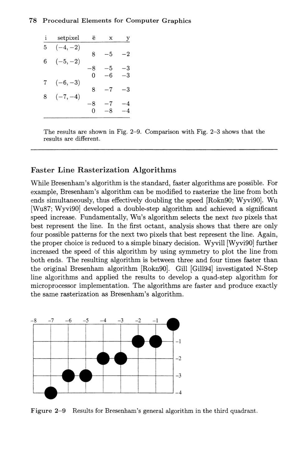
Text
PROCEDURAL
ELEMENTS
FOR
COMPUTER
GRAPHICS
Second Edition
David F. Rogers
Professor of Aerospace Engineering
United States Naval Academy, Annapolis, Md.
WCB
McGraw-Hill
Boston, Massachusetts
Burr Ridge, Illinois Dubuque, Iowa Madison, Wisconsin
New York, New York San Francisco* California St. Louis, Missouri
WCB/McGraw-Hill
A Division of The McGraw-Hill Companies
Copyright © 1998 by The McGraw-Hill Companies, Inc. All rights reserved. Previous
edition(s) © 1985. Printed in the United States of America. Except as permitted
under the United States Copyright Act of 1976, no part of this publication may be
reproduced or distributed in any form or by any means, or stored in a data base or
retrieval system, without the prior written permission of the publisher.
This book is printed on acid-free paper.
23456789 BKM BKM 909876543210
ISBN 0-07-053548-5
Editorial director: Kevin Kane
Publisher: Tom Casson
Executive editor: Elizabeth A. Jones
Senior developmental editor: Kelley Butcher
Marketing manager: John Wannemacher
Project manager: Kari Geltemeyer
Production supervisor: Heather D. Burbridge
Senior designer: Laurie J. Entringer
Compositor: NAR Associates
Cover illustration credits:
Front Cover: Image created by Peter Kipfer and Frangois Sillion using a hierarchical
radiosity lighting simulation developed in the iMAGIS project GRAVIR/IMAG-INRIA
(Grenoble, France) in consultation with the author (Annapolis, MD). The entire project
was accomplished electronically from initial concept to final images. The image
incorporates the simple block structure from the first edition to illustrate the vast
improvements in rendering capability. There are 287 initial surfaces in 157 clusters. Adaptive
subdivision resulted in 1,861,974 links. Image Copyright © 1997 Frangois Sillion, Peter
Kipfer and David F. Rogers. All rights reserved.
Back cover: The image shows an adaptively subdivided coarse mesh, created with
a factor of 30 increase in the error metric, superimposed over the front cover image.
Image Copyright © 1997 Frangois Sillion, Peter Kipfer and David F. Rogers. All rights
reserved.
Library of Congress Cataloging-in-Publication Data
Rogers, David F.
Procedural elements for computer graphics / David F. Rogers - -
2nd ed.
p. cm.
Includes bibliographical references and index.
ISBN 0-07-053548-5
1. Computer graphics. I. Title.
T385.R63 1998
006.6 - - dc21 97-13301
http://www.mhhe.com
This one is for my wife
and best friend
Nancy A. (Nuttall) Rogers
without whom this book
and all the others
would not have been possible.
CONTENTS
Preface xv
Preface to the First Edition xvii
Chapter 1 Introduction To Computer Graphics 1
1-1 Overview of Computer Graphics 1
Representing Pictures 2
Preparing Pictures for Presentation 2
Presenting Previously Prepared Pictures 3
1-2 Raster Refresh Graphics Displays 6
Frame Buffers 7
1-3 Cathode Ray Tube Basics 11
Color CRT Raster Scan Monitors 13
1-4 Video Basics 14
American Standard Video 14
High Definition Television 17
1-5 Flat Panel Displays 17
Flat CRT 17
Plasma Display 18
Electroluminescent Display 21
Liquid Crystal Display 21
1-6 Hardcopy Output Devices 25
Electrostatic Plotters 25
Ink Jet Plotters 26
Thermal Plotters 28
Dye Sublimation Printers 30
Pen and Ink Plotters 31
Laser Printers 34
Color Film Cameras 36
1-7 Logical Interactive Devices 37
The Locator Function 38
vii
viii Contents
The Valuator Function 39
The Buttom or Choice Function 39
The Pick Function 39
1-8 Physical Interactive Devices 39
Tablets 40
Touch Panels 41
Control Dials 41
Joystick 42
Trackball 42
Mouse 44
Function Switches 44
Light Pen 45
Spaceball 46
Data Glove 46
Simulation of Alternate Devices 47
1-9 Data Generation Devices 49
Scanners 49
Three-dimensional Digitizers 50
Motion Capture 51
1-10 Graphical User Interfaces 52
Cursors 54
Radio Buttons 55
Valuators 55
Scroll Bars 56
Grids 56
Dialog Boxes 57
Menus 58
Icons 59
Sketching 60
3-D Interaction 63
summary 64
Chapter 2 Raster Scan Graphics 65
2-1 Line Drawing Algorithms 65
2-2 Digital Differential Analyzer 66
2-3 Bresenham's Algorithm 70
Integer Bresenham's Algorithm 74
General Bresenham's Algorithm 75
Faster Line Rasterization Algorithms 78
2-4 Circle Generation—Bresenham's Algorithm 79
2-5 Ellipse Generation 88
2-6 General Function Rasterization 95
2-7 Scan Conversion—Generation of the Display 97
Real-time Scan Conversion 97
A Simple Active Edge List Using Pointers 99
Contents ix
A Sorted Active Edge List 99
An Active Edge List Using a Linked List 101
Updating the Linked List 102
2-8 Image Compression 104
Run-length Encoding 104
Area Image Compression 107
2-9 Displaying Lines, Characters and Polygons 111
Line Display 111
Character Display 113
Solid Area Scan Conversion 114
2-10 Polygon Filling 115
Scan-converting Polygons 115
2-11 A Simple Parity Scan Conversion Algorithm 118
2-12 Ordered Edge List Polygon Scan Conversion 121
A Simple Ordered Edge List Algorithm 122
More Efficient Ordered Edge List Algorithms 123
2-13 The Edge Fill Algorithm 126
2-14 The Edge Flag Algorithm 131
2-15 Seed Fill Algorithms 133
A Simple Seed Fill Algorithm 134
A Scan Line Seed Fill Algorithm 137
2-16 Fundamentals of Antialiasing 142
Supersampling 143
Straight Lines 144
Polygon Interiors 151
Simple Area Antialiasing 152
The Convolution Integral and Antialiasing 156
Filter Functions 159
2-17 Halftoning 161
Patterning 161
Thresholding and Error Distribution 165
Ordered dither 169
Chapter 3 Clipping 175
3-1 Two-dimensional Clipping 175
A Simple Visibility Algorithm 176
End Point Codes 177
3-2 Cohen-Sutherland Subdivision Line
Clipping Algorithm 181
3-3 Midpoint Subdivision Algorithm 187
3-4 Two-dimensional Line Clipping for
Convex Boundaries 192
Partially Visible Lines 193
3-5 Cyrus-Beck Algorithm 196
Partially Visible Lines 199
x Contents
Totally Visible Lines 201
Totally Invisible Lines 201
Formal Statement of Cyrus-Beck Algorithm 203
Irregular Windows 207
3-6 Liang-Barsky Two-dimensional Clipping 208
Comparison with the Cyrus-Beck Algorithm 212
3-7 Nicholl-Lee-Nicholl Two-dimensional Clipping 217
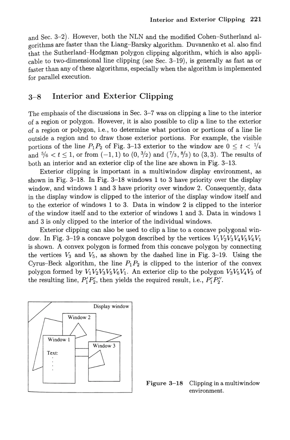
3-8 Interior and Exterior Clipping 221
3-9 Identifying Convex Polygons and Determining the
Inward Normal 222
3-10 Splitting Concave Polygons 225
3-11 Three-dimensional Clipping 228
3-12 Three-dimensional Midpoint Subdivision Algorithm 231
3-13 Three-dimensional Cyrus-Beck Algorithm 233
3-14 Liang-Barsky Three-dimensional Clipping 239
3-15 Clipping in Homogeneous Coordinates 243
The Cyrus-Beck Algorithm 243
The Liang-Barsky Algorithm 245
3-16 Determining the Inward Normal and
Three-dimensional Convex Sets 248
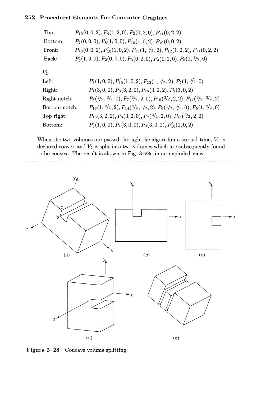
3-17 Splitting Concave Volumes 250
3-18 Polygon Clipping 253
3-19 Reentrant Polygon Clipping—
Sutherland-Hodgman Algorithm 253
Determining the Visibility of a Point 355
Line Intersections 257
The Algorithm 258
3-20 Liang-Barsky Polygon Clipping 265
Entering and Leaving Vertices 265
Turning Vertices 267
Development of the Algorithm 268
Horizontal and Vertical Edges 271
The Algorithm 272
3-21 Concave Clipping Regions—
Weiler-Atherton Algorithm 276
Special Cases 282
3-22 Character Clipping 286
Chapter 4 Visible Lines and Visible Surfaces 287
4-1 Introduction 287
4-2 Floating Horizon Algorithm 289
Upper Horizon 290
Lower Horizon 290
Function Interpolation 291
Aliasing 295
Contents xi
4-3
4-4
4-5
4-6
4-7
4-8
4-9
4-10
4-11
4-12
4-13
4-14
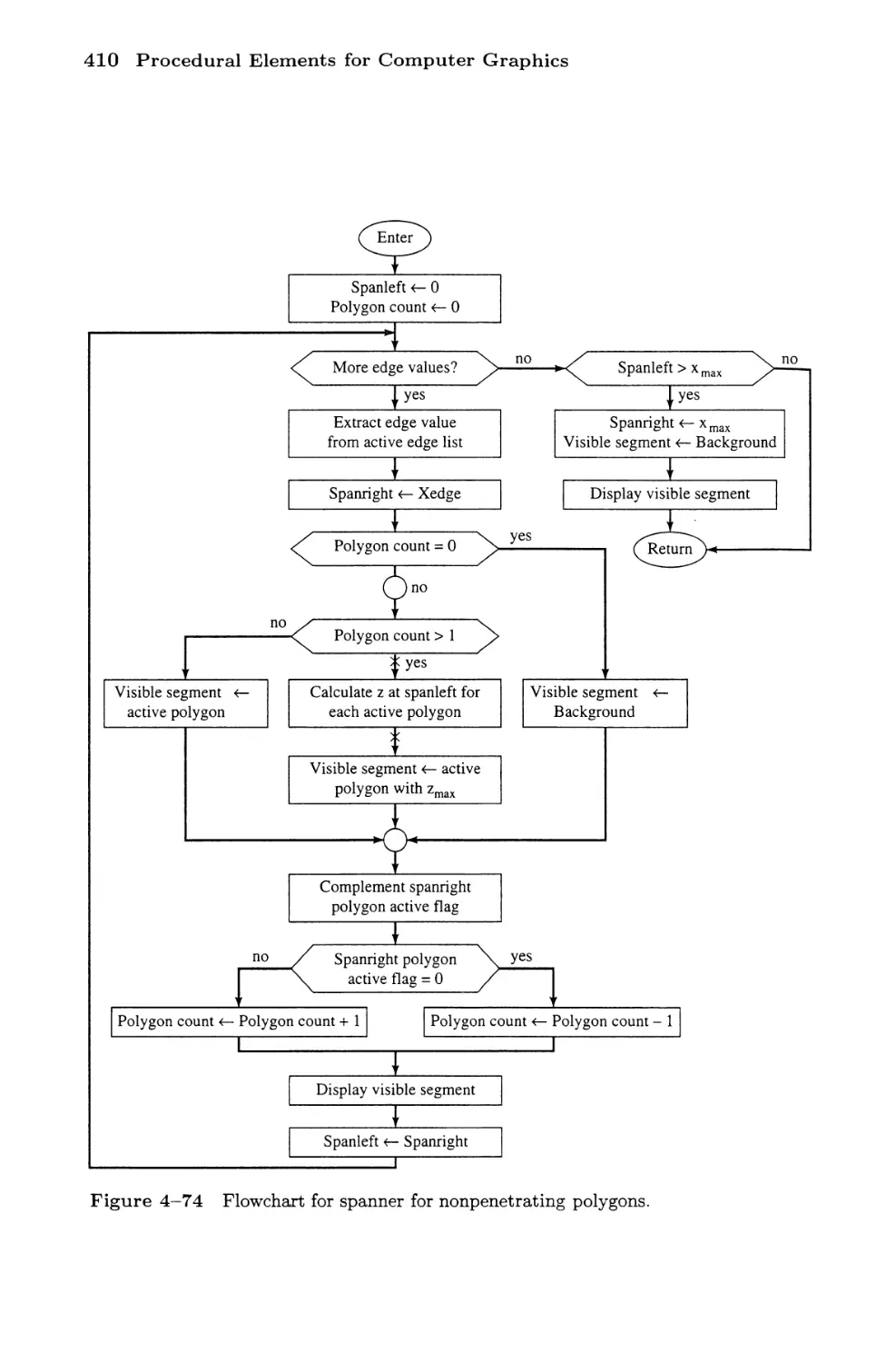
4-15
4-16
4-17
4-18
The Algorithm
Cross-hatching
Roberts Algorithm
Volume Matrices
Plane Equations
Viewing Transformations and Volume Matrices
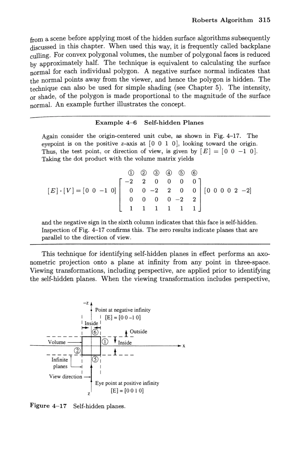
Self-hidden Planes
Lines Hidden by Other Volumes
Penetrating Volumes
Totally Visible Lines
The Algorithm
Waxnock Algorithm
Quadtree Data Structure
Subdivision Criteria
The Relationship of a Polygon to a Window
Hierarchical Application of
Polygon-Window Relations
Finding Surrounder Polygons
The Basic Algorithm
Appel's Algorithm
The Haloed Line Algorithm
Weiler-Atherton Algorithm
A Subdivision Algorithm for Curved Surfaces
Z-BufFer Algorithm
Incrementally Calculating the Depth
Hierarchical Z-Buffer
The A-Buffer Algorithm
List Priority Algorithms
The Newell-Newell-Sancha Algorithm
Implementing the Tests
Binary Space Partitioning
The Schumaker Algorithm
Binary Space Partition Trees
Constructing the BSP Tree
BSP Tree Traversal
Culling
Summary
Scan Line Algorithms
Scan Line Z-Buffer Algorithm
A Spanning Scan Line Algorithm
Invisible Coherence
An Object Space Scan Line Algorithm
Scan Line Algorithms for Curved Surfaces
Octrees
Octree Display
295
303
303
306
308
311
314
318
327
327
330
343
345
347
349
354
355
357
363
366
370
374
375
378
383
384
387
389
390
393
393
395
395
398
400
400
401
402
406
415
416
417
421
424
xii Contents
4-19
4-20
4-21
5-1
5-2
5-3
5-4
5-5
5-6
5-7
5-8
5-9
5-10
5-11
Linear Octrees
Manipulation of Octrees
Boolean Operations
Finding Neighboring Voxels
Marching Cubes
Ambiguous faces
A Visible Surface Ray Tracing Algorithm
Bounding Volumes
Clusters
Constructing the Cluster Tree
Priority Sort
Spatial Subdivision
Uniform Spatial Subdivision
Nonuniform Spatial Subdivision
Ray-Object Intersections
Opaque Visible Surface Algorithm
Summary
Rendering
Introduction
Illumination Models
A Simple Illumination Model
Specular Reflection
The Halfway Vector
Determining the Surface Normal
Determining the Reflection Vector
Gouraud Shading
Phong Shading
Fast Phong Shading
A Simple Illumination Model with Special Effects
A Physically Based Illumination Model
Energy and Intensity
Physically Based Illumination Models
The Torrance-Sparrow Surface Model
Wavelength Dependence—the Fresnel Term
Color Shift
Physical Characteristics of Light Sources
Transparency
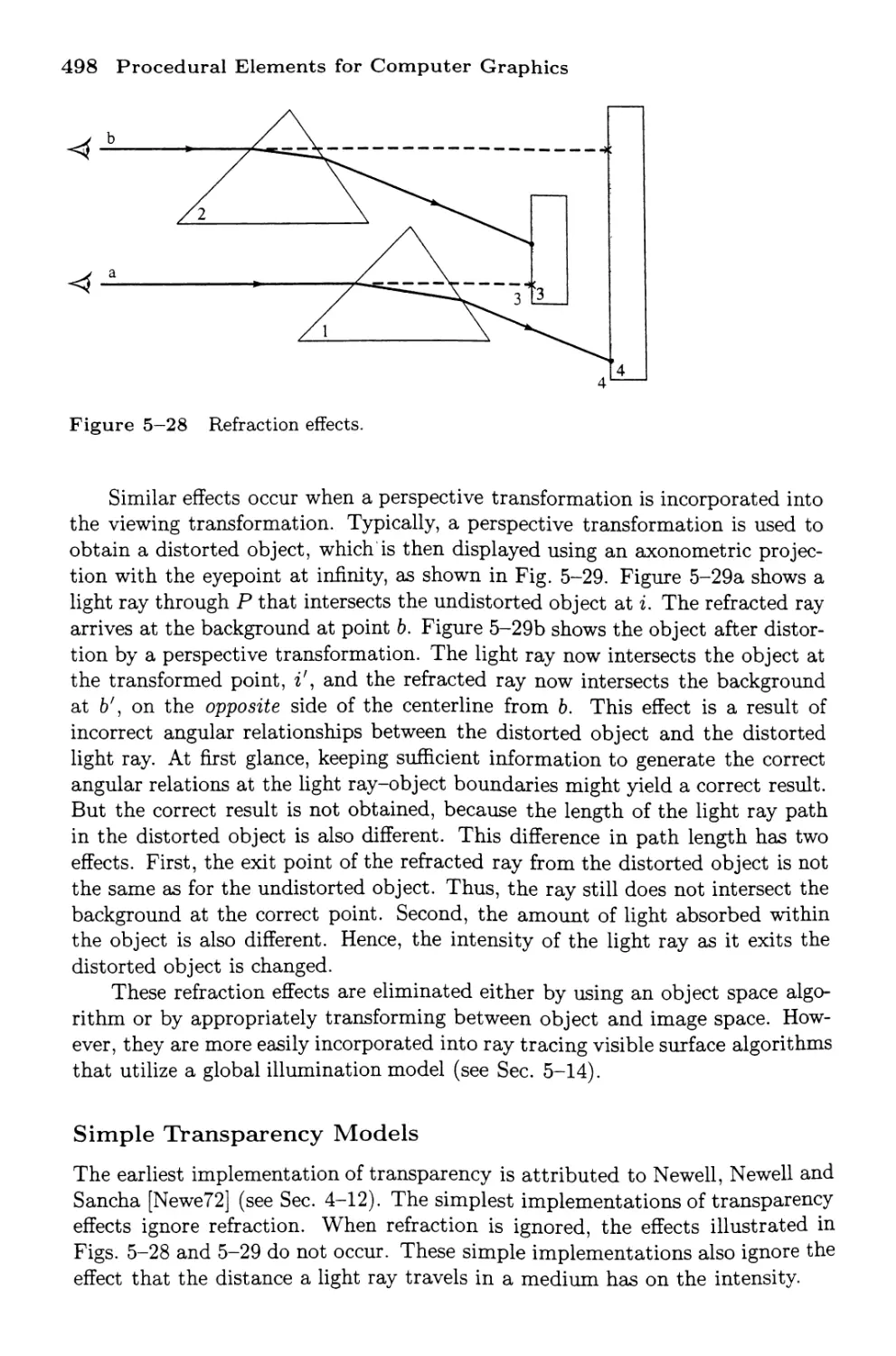
Refraction Effects in Transparent Materials
Simple Transparency Models
Z-Buffer Transparency
Pseudotransparency
Shadows
The Scan Conversion Shadow Algorithms
Multiple-pass Visible Surface
426
426
426
427
427
429
432
435
439
440
440
441
442
445
447
451
456
457
457
460
461
462
465
468
470
474
476
482
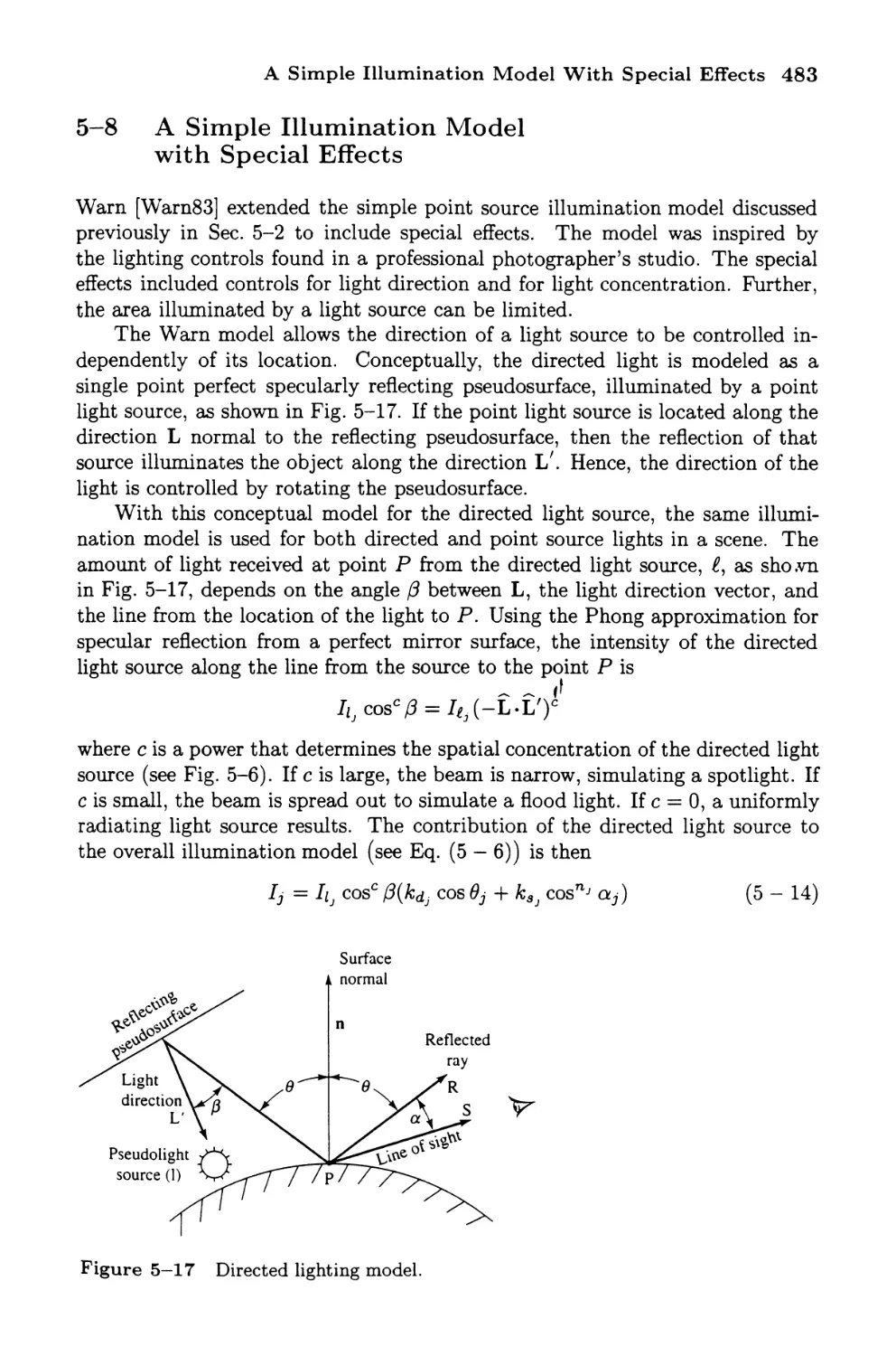
483
484
485
487
488
491
492
494
496
497
498
500
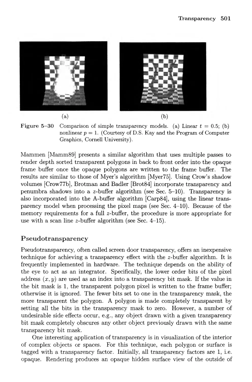
501
502
506
Contents xiii
Shadow Algorithms
The Shadow Volume Algorithms
Penumbra Shadows
Ray Tracing Shadow Algorithms
12 Texture
Mapping Functions
Two-part Texture Mapping
Environment Mapping
Bump Mapping
Procedural Textures
Texture Antialiasing
Mipmapping (Image Pyramids)
Summed Area Tables
13 Stochastic Models
14 A Global Illumination Model Using Ray Tracing
15 A More Complete Global Illumination Model Using
Ray Tracing
16 Advances in Ray Tracing
Cone Tracing
Beam Tracing
Pencil Tracing
Stochastic Sampling
Ray Tracing from the Light Source
17 Radiosity
Enclosures
Form Factors
The Hemicube
Rendering
Substructuring
Progressive Refinement
Sorting
The Ambient Contribution
Adaptive Subdivision
Hemicube Inaccuracies
Alternatives to the Hemicube
Hierarchical Radiosity and Clustering
Radiosity for Specular Environments
The Rendering Equation
18 Combined Ray Tracing and Radiosity
The Extended Two-pass Algorithm
19 Color
Chromaticity
Tristimulus Theory of Color
Color Primary Systems
Color Matching Experiment
508
509
514
517
517
525
528
531
534
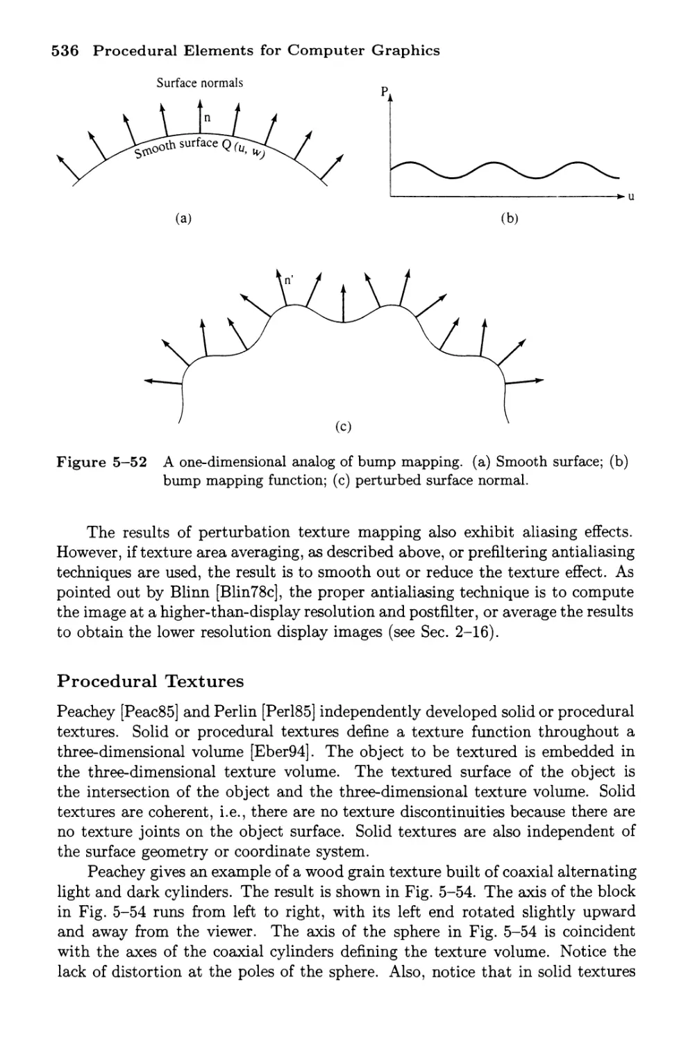
536
539
542
544
545
548
563
565
565
566
567
567
570
571
573
575
577
582
584
585
586
586
587
589
592
594
596
597
598
602
602
603
605
606
606
xiv Contents
5-20
5-21
5-22
Appendix
References
Index
Chromaticity Diagrams
The 1931 CIE Chromaticity Diagram
Uniform Color Spaces
Gamut Limitations
Transformations Between Color Systems
NTSC Color System
Color Cubes
The CMYK Color System
The Ostwald Color System
The HSV Color System
The HLS Color System
The Munsell Color System
The Pantone® System
Gamma Correction
Color Image Quantization
The Bit Cutting Algorithm
The Popularity Algorithm
The Median Cut Algorithm
Octree Quantization
Sequential Scalar Quantization
Other Quantization Algorithms
Color Reproduction
Offset Printing
Color Separation
Tone Reproduction
Gray Balance
The Black Separation
Quantization Effects
Calibration
Gamut Mapping
Specialty Rendering Techniques
Duotone Printing
Rendering Natural Objects
Particle Systems
Problems and Projects
609
611
615
616
618
621
622
623
623
624
627
630
631
631
633
634
635
637
640
644
647
648
649
649
649
650
650
650
650
651
654
654
656
656
657
665
695
PREFACE
In the preface to the first edition I wrote "Computer graphics is now a mature
discipline." Little did I or anyone else anticipate the developments of the last dozen
years. Then, ray tracing was an active research topic — now there are freely
available programs for personal computers; radiosity was just on the horizon —
today commercially rendering systems commonly use this technique; texture was
a software application — today hardware texture acceleration is common place;
color image quantization algorithms were certainly available in the computer
graphics community, but today downloading an image from the World Wide
Web depends on color image quantization. The list goes on. Computer graphics
is thoroughly integrated into our daily lives, across fields as diverse as
advertising, entertainment, medicine, education, science, engineering, navigation, etc. In
fact, most computer programs, including the most popular operating systems,
have a graphical user interface.
The present volume represents a major rewrite of the first edition. As a
result, it is nearly twice the size of the original volume. Major new additions
include a discussion of graphical user interfaces, an expanded discussion of line,
circle and ellipse drawing and image compression algorithms. New clipping
algorithms for lines and polygons are presented. In particular, the Liang-Barsky
and Nicholl-Lee-Nicholl clipping algorithms are now discussed along with the
classical Cohen-Sutherland, midpoint, Cyrus-Beck and Sutherland-Hodgman
clipping algorithms.
The chapter on visible surface algorithms now includes sections on the Appel,
haloed line and A-buffer algorithms, along with discussions of the binary space
partitioning (BSP), octree and marching cubes algorithms. The discussion of
the visible surface ray tracing algorithm is considerably expanded.
The rendering chapter is significantly enhanced. It now includes expanded
discussions of physically based illumination models, transparency, shadows and
textures. More recent advances in ray tracing, for example, cone, beam, pencil
and stochastic ray tracing, are included along with a detailed discussion of the
fundamentals of radiosity. The section on color is expanded to include uniform
color spaces and a more detailed discussion of gamma correction. Sections on
color image quantization and color reproduction for print media are included.
xv
xvi Procedural Elements for Computer Graphics
The book is suitable for use by professional programmers, engineers and
scientists. A course in computer graphics at either the senior undergraduate or
first year graduate level that emphasizes rendering techniques will benefit from
the book. Combining it with its companion volume, Mathematical Elements
for Computer Graphics, allows increasing the scope of the course to include
manipulative transformations and curves and surfaces. The book retains the
detailed worked examples from the first edition as well as presenting new ones
— a total of 90 worked examples. An adequate background is provided by college
level mathematics and knowledge of a higher-level programming language.
No computer graphics book is complete without algorithms. There are three
types of algorithms presented in the book. The first is a narrative description
often presented in list form; the second is a detailed procedural description of
the algorithm, while the third is a more formal presentation using pseudocode.
Although many books now present algorithms in C, I resisted this temptation.
I believe that actually implementing an algorithm yields better understanding
and appreciation of the nuances of the algorithm which no book can cover.
Furthermore, as the algorithm is implemented additional efficiencies specific to the
implementation language frequently suggest themselves. For those algorithms
presented in pseudocode, the actual implementation is relatively straightforward.
No book is ever written without the assistance of many individuals. Thanks
are expressed to my colleagues who read various parts of the manuscript. John
Dill and his students read all of Chapter 3 on clipping and made many valuable
comments. Paul Heckbert read both the sections on color image quantization and
textures. Both sections are much the better for his comments. Maureen Stone
lent her expertise on color reproduction. Eric Haines commented extensively on
the ray tracing sections. I particularly enjoyed the ensuing discussions. John
Wallace read the section on radiosity and set me straight on one or two key
points. However, any errors are mine alone.
Special thanks are due my colleagues Frangois Sillion and Peter Kipfer at
the iMAGIS project in Grenoble, France, who created the cover image to an
impossibly short deadline using hierarchical radiosity software developed under
the direction of Frangois Sillion and George Drettakis. You enthusiastically made
all the changes that I requested! It was great working with you.
My editor of more than two and a half decades, B.J. Clark, has now left for
other pastures. Without his initial faith in a young academic who wanted to
do a book on computer graphics, and his gentle encouragement over the years,
none of this would have happened. Thanks are due Fred Eckardt and his crew
at Fine Line Illustrations for their efforts in creating the line art. They even
trusted me with the original files. The production crew at McGraw-Hill — Kari
Geltemeyer, Laurie Entringer and Heather Burbridge — did an outstanding job.
Last, but certainly not least, a very special thanks is due my wife Nancy for
not only her long term patience with my need to write, but especially for the
outstanding job of copy editing, proof reading and typesetting. I think you now
qualify as a TEXpert.
David F. Rogers
PREFACE TO THE FIRST EDITION
Computer graphics is now a mature discipline. Both hardware and software
are available that facilitate the production of graphical images as diverse as line
drawings and realistic renderings of natural objects. A decade ago the hardware
and software to generate these graphical images cost hundreds of thousands of
dollars. Today, excellent facilities are available for expenditures in the tens of
thousands of dollars and lower performance, but in many cases adequate
facilities are available for tens of hundreds of dollars. The use of computer graphics
to enhance information transfer and understanding is endemic in almost all
scientific and engineering disciplines. Today, no scientist or engineer should be
without a basic understanding of the underlying principles of computer
graphics. Computer graphics is also making deep inroads into the business, medical,
advertising, and entertainment industries. The presence in the boardroom of
presentation slides prepared using computer graphics facilities as well as more
commonplace business applications is considered the norm. Three-dimensional
reconstructions using data obtained from CAT scans is becoming commonplace
in medical applications. Television as well as other advertising media are now
making frequent use of computer graphics and computer animation. The
entertainment industry has embraced computer graphics with applications as diverse
as video games and full-length feature films. Even art is not immune, as
evidenced by some of the photos included in this book.
It is almost a decade now since the appearance of the companion volume
to this book, Mathematical Elements for Computer Graphics. During that time
significant strides in raster scan graphics have been made. The present volume
concentrates on these aspects of computer graphics. The book starts with an
introduction to computer graphics hardware with an emphasis on the
conceptual understanding of cathode ray tube displays and of interactive devices. The
following chapters look at raster scan graphics including line and circle drawing,
polygon filling, and antialiasing algorithms; two- and three-dimensional clipping
including clipping to arbitrary convex volumes; hidden-line and hidden-surface
xvii
xviii Procedural Elements for Computer Graphics
algorithms including ray tracing; and finally, rendering, the art of making
realistic pictures, including local and global illumination models, texture, shadows,
transparency, and color effects. The book continues the presentation technique
of its predecessor. Each thorough topic discussion is followed by presentation of
a detailed algorithm or a worked example, and where appropriate both.
The material in the book can be used in its entirety for a semester-long
first formal course in computer graphics at either the senior undergraduate or
graduate level with an emphasis on raster scan graphics. If a first course in
computer graphics based on the material in the companion volume Mathematical
Elements for Computer Graphics is presented, then the material in this book is
ideal for a second course. This is the way it is used by the author. If broader
material coverage in a single-semester course is desired, then the two volumes
can be used together. Suggested topic coverage is: Chapter 1 of both volumes,
followed by Chapters 2 and 3 with selected topics from Chapter 4 of
Mathematical Elements for Computer Graphics, then selected topics from Chapter 2
(e.g., 2-1 to 2-5, 2-7, 2-15 to 2-19, 2-22, 2-23, 2-28), Chapter 3 (e.g., 3-1, 3-2,
3-4 to 3-6, 3-9, 3-11, 3-15, 3-16), Chapter 4 (e.g., 4-1, part of 4-2 for backplane
culling, 4-3, 4-4, 4-7, 4-9, 4-11, 4-13), and Chapter 5 (e.g., 5-1 to 5-3, 5-5, 5-6,
5-14) of the present volume. The book is also designed to be useful to
professional programmers, engineers, and scientists. Further, the detailed algorithms
and worked examples make it particularly suitable for self-study at any level.
Sufficient background is provided by college level mathematics and a knowledge
of a higher-level programming language. Some knowledge of data structures is
useful but not necessary.
There are two types of algorithms presented in the book. The first is a
detailed procedural description of the algorithm, presented in narrative style.
The second is more formal and uses an algorithmic 'language' for presentation.
Because of the wide appeal of computer graphics, the choice of an algorithmic
presentation language was especially difficult. A number of colleagues were
questioned as to their preference. No consensus developed. Computer science faculty
generally preferred PASCAL but with a strong sprinkling of C. Industrial
colleagues generally preferred FORTRAN for compatibility with existing software.
The author personally prefers BASIC because of its ease of use. Consequently,
detailed algorithms are presented in pseudocode. The pseudocode used is based
on extensive experience teaching computer graphics to classes that do not
enjoy knowledge of a common programming language. The pseudocode is easily
converted to any of the common computer languages. An appendix discusses
the pseudocode used. The pseudocode algorithms presented in the book have
all been either directly implemented from the pseudocode or the pseudocode has
been derived from an operating program in one or more of the common
programming languages. Implementations range from BASIC on an Apple He to PL1 on
an IBM 4300 with a number of variations in between. A suit of demonstration
programs in available from the author.
A word about the production of the book may be of interest. The book
was computer typeset using the TEX typesetting system at TYX Corporation
PREFACE TO THE FIRST EDITION xix
of Reston, Virginia. The manuscript was coded directly from handwritten copy.
Galleys and two sets of page proofs were produced on a laser printer for editing
and page makeup. Final reproduction copy ready for art insertion was
produced on a phototypesetter. The patience and assistance of Jim Gauthier and
Mark Hoffman at TYX while the limits of the system were explored and
solutions to all the myriad small problems found is gratefully acknowledged. The
outstanding job done by Louise Bohrer and Beth Lessels in coding the
handwritten manuscript is gratefully acknowledged. The usually fine McGraw-Hill
copyediting was supervised by David Damstra and Sylvia Warren.
No book is ever written without the assistance of many individuals. The
book is based on material prepared for use in a graduate level course given at
the Johns Hopkins University Applied Physics Laboratory Center beginning in
1978. Thanks are due the many students in this and other courses from whom
I have learned so much. Thanks are due Turner Whitted who read the original
outline and made valuable suggestions. Thanks are expressed to my colleagues
Pete Atherton, Brian Barsky, Ed Catmull, Rob Cook, John Dill, Steve Hansen,
Bob Lewand, Gary Meyer, Alvy Ray Smith, Dave Warn, and Kevin Weiler, all of
whom read one or more chapters or sections, usually in handwritten manuscript
form, red pencil in hand. Their many suggestions and comments served to make
this a better book. Thanks are extended to my colleagues Linda Rybak and
Linda Adlum who read the entire manuscript and checked the examples. Thanks
are due three of my students: Bill Meier who implemented the Roberts algorithm,
Gary Boughan who originally suggested the test for convexity discussed in Sec. 3-
7, and Norman Schmidt who originally suggested the polygon splitting technique
discussed in Sec. 3-8. Thanks are due Mark Meyerson who implemented the
splitting algorithms and assured that the technique was mathematically well
founded. The work of Lee Billow and John Metcalf who prepared all the line
drawings is especially appreciated.
Special thanks are due Steve Satterfield who read and commented on all
800 handwritten manuscript pages. Need more be said!
Special thanks are also due my eldest son Stephen who implemented all
of the hidden surface algorithms in Chapter 4 as well as a number of other
algorithms throughout the book. Our many vigorous discussions served to clarify
a number of key points.
Finally, a very special note of appreciation is extended to my wife Nancy
and to my other two children, Karen and Ransom, who watched their husband
and father disappear into his office almost every weeknight and every weekend
for a year and a half with never a protest. That is support! Thanks.
t
David F. Rogers
CHAPTER
ONE
INTRODUCTION TO
COMPUTER GRAPHICS
Today computers and computer graphics are an integral part of daily life for
many people. Computer graphics is in daily use in the fields of science,
engineering, medicine, entertainment, advertising, the graphic arts, the fine arts,
business, education and training to mention only a few. Today, learning to program
involves at least an exposure to two- and in most cases three-dimensional
computer graphics. Even the way we access our computer systems is in most cases
now graphically based. As an illustration of the growth in computer graphics,
consider that in the early 1970s SIGGRAPH, the annual conference of the
Association of Computing Machinery's (ACM) Special Interest Group on GRAPHics,
involved a few hundred people. Today, the annual conference draws tens of
thousands of participants.
1-1 Overview of Computer Graphics
Computer graphics is a complex and diversified technology. To begin to
understand the technology, it is necessary to subdivide it into manageable parts. This
can be accomplished by considering that the end product of computer graphics
is a picture. The picture may, of course, be used for a large variety of purposes;
e.g., it may be an engineering drawing, an exploded parts illustration for a service
manual, a business graph, an architectural rendering for a proposed construction
or design project, an advertising illustration, an image for a medical procedure
or a single frame for an animated movie. The picture is the fundamental cohesive
concept in computer graphics. We must therefore consider how:
Pictures are represented in computer graphics
Pictures are prepared for presentation
Previously prepared pictures are presented
1
2 Procedural Elements for Computer Graphics
Interaction with the picture is accomplished
Here 'picture' is used in its broadest sense, to mean any collection of lines, points,
text, etc. displayed on a graphics device.
Representing Pictures
Although many algorithms accept picture data as polygons or edges, each
polygon or edge can in turn be represented by points. Points, then, are the
fundamental building blocks of picture representation. Of equal fundamental importance
is the algorithm, which explains how to organize these points. To illustrate this,
consider a unit square in the first quadrant. The unit square can be represented
by its four corner points (see Fig. 1-1):
Pi (0,0) P2(1,0) P3(l,l) P4(0,1)
An associated algorithmic description might be
Connect P1P2P3P4P1 in sequence
The unit square can also be described by its four edges
E1 = PiP2 E2 = P2P3 E3 = P3P4 £4 = P4P1
Here, the algorithmic description is
Connect E1E2E3E4 in sequence
Finally, either the points or edges can be used to describe the unit square as a
single polygon, e.g.
Si = P1P2P3P4P1 or Si = E1E2E3E4
The fundamental building blocks, i.e., points, can be represented as either pairs
or triplets of numbers, depending on whether the data are two- or
three-dimensional. Thus, (#1,7/1) or (a?i,yi,zi) represent a point in either two- or three-
dimensional space. Two points represent a line or edge, and a collection of
three or more points a polygon. The representation of curved lines is usually
accomplished by approximating them by connected short straight line segments.
The representation of textual material is quite complex, involving in many
cases curved lines or dot matrices. Fundamentally, textual material is again
represented by collections of lines and points and an organizing algorithm. Unless
the user is concerned with pattern recognition, the design of special character
fonts or the design of graphic hardware, he or she need not be concerned with
these details.
Preparing Pictures for Presentation
Pictures ultimately consist of points and a drawing algorithm to display them.
This information is generally stored in a file before it is used to present the
Overview of Computer Graphics 3
l
1.0 <
E4
P,<
L
Pf
f
\
E3 .
s,
^
E2
u_
»
0 Ej 1.0 Figure 1—1 Picture data descriptions.
picture; this file is called a data base. Very complex pictures require very complex
data bases, which require a complex algorithm to access them. These complex
data bases contain data organized in various ways, e.g., ring structures, B-tree
structures, quadtree structures, etc., generally referred to as a data structure.
The data base itself may contain pointers, substructures and other nongraphic
data. The design of these data bases and the algorithms which access them is an
ongoing topic of research, a topic which is clearly beyond the scope of this text.
However, many computer graphics applications involve much simpler pictures,
for which the user can readily invent simple data structures which can be easily
accessed. The simplest is, of course, a lineal list. Surprisingly, this simplest of
data structures is quite adequate for many reasonably complex pictures.
Because points are the basic building blocks of a graphic data base, the
fundamental operations for manipulating these points are of interest. There are
three fundamental operations when treating a point as a (geometric) graphic
entity: move the beam, pen, cursor, plotting head (hereafter called the cursor)
invisibly to the point; draw a visible line to a point from an initial point; or
display a dot at that point. Fundamentally there are two ways to specify the
position of a point: absolute coordinates, or relative (incremental) coordinates.
In relative, or incremental, coordinates, the position of a point is defined by
giving the displacement of the point with respect to the previous point. All
computer graphics software is based on these fundamental operations.
Presenting Previously Prepared Pictures
The data used to prepare the picture for presentation is rarely the same as that
used to present the picture. The data used to present the picture is frequently
called a display file. The display file represents some portion, view or scene of
the picture represented by the total data base. The displayed picture is
usually formed by rotating, translating, scaling and performing various projections
on the data. These basic orientation or viewing preparations are generally
performed using a 4 x 4 transformation matrix, operating on the data represented
in homogeneous coordinates (see [Roge90a]).
4 Procedural Elements for Computer Graphics
Hidden line or hidden surface removal (see Chapter 4), shading,
transparency, texture or color effects (see Chapter 5) may be added before final
presentation of the picture. If the picture represented by the entire data base is not
to be presented, the appropriate portion must be selected. This is a process
called clipping. Clipping may be two- or three-dimensional, as appropriate. In
some cases, the clipping window, or volume, may have holes in it or may be
irregularly shaped. Clipping to standard two- and three-dimensional regions is
frequently implemented in hardware. A complete discussion of these effects is
given in Chapter 3.
Two important concepts associated with presenting a picture are windows
and viewports. Windowing is the process of extracting a portion of a data base by
clipping the data base to the boundaries of the window. For large data bases,
performance of the windowing or the clipping operation in software generally is
sufficiently time consuming that real-time interactive graphics is not possible. Again,
sophisticated graphics devices perform this function in special-purpose hardware
or microcode. Clipping involves determining which lines or portions of lines in
the picture lie outside the window. Those lines or portions of lines are then
discarded and not displayed; i.e., they are not passed on to the display device.
In two dimensions, a window is specified by values for the left, right, bottom
and top edges of a rectangle. The window edge values are specified in user
or world coordinates, i.e., the coordinates in which the data base is specified.
Floating point numbers are usually used.
Clipping is easiest if the edges of the rectangle are parallel to the coordinate
axes. Such a window is called a regular clipping window. Irregular windows are
Line partially within window:
part from a - b displayed;
part from b - c not displayed
Line entirely
within
window:
entire line
displayed
Line partially within
window: part from b - c
displayed; parts a-b, c -d
not displayed
Line entirely
outside of
window: not
displayed
Figure 1-2 Two-dimensional windowing (clipping).
Overview of Computer Graphics 5
also of interest for many applications (see Chapter 3). Two-dimensional
clipping is represented in Fig. 1-2. Lines are retained, deleted or partially deleted,
depending on whether they are completely or partially within or without the
window. In three dimensions, a regular window or clipping volume consists of a
rectangular parallelepiped (a box) or, for perspective views, a frustum of vision.
A typical frustum of vision is shown in Fig 1-3. In Fig. 1-3 the near (hither)
boundary is at TV, the far (yon) boundary at F and the sides at SL, SR, ST
and SB.
A viewport is an area of the display device on which the window data is
presented. A two-dimensional regular viewport is specified by giving the left,
right, bottom and top edges of a rectangle. Viewport values may be given in
actual physical device coordinates. When specified in actual physical device
coordinates, they are frequently given using integers. Viewport coordinates may be
normalized to some arbitrary range, e.g., 0 < x < 1.0, 0 < y < 1.0, and specified
by floating point numbers. The contents of a single window may be displayed in
multiple viewports on a single display device, as shown in Fig. 1-4. Keeping the
proportions of the window and viewport(s) the same prevents distortion. The
mapping of windowed (clipped) data onto a viewport involves translation and
scaling (see [Roge90a]).
An additional requirement for most pictures is the presentation of
alphanumeric or character data. There are, in general, two methods of generating
characters — software and hardware. If characters are generated in software using
lines, they are treated in the same manner as any other picture element. In fact,
this is necessary if they are to be clipped and then transformed along with other
picture elements. However, many graphics devices have hardware character
generators. When hardware character generators are used, the actual characters
are generated just prior to being drawn. Up until this point they are treated
Figure 1-3 Three-dimensional frustum of vision.
6 Procedural Elements for Computer Graphics
World coordinate
data base
Window
Display device
Viewport A
Viewport B
Figure 1—4 Multiple viewports displaying a single window.
as character codes. Hardware character generation yields significant efficiencies.
However, it is less flexible than software character generation, because it does not
allow for clipping or general transformation; e.g., usually only limited rotations
and sizes are possible.
Before discussing how we interact with the picture, we first look at some
fundamentals of cathode ray tubes and how they are used in computer graphics, and
discuss some of the physical output devices that are used in computer graphics.
1-2 Raster Refresh Graphics Displays
Although storage tube and calligraphic line drawing refresh graphics displays,
sometimes called random line scan displays, are still occasionally used in
computer graphics,' the raster refresh graphics display is the predominant graphics
display. On both the storage tube and the calligraphic line drawing refresh
display, a straight line can be drawn directly from any addressable point to any
other addressable point. In contrast, the raster CRT graphics display is a point
plotting device. A raster graphics device can be considered a matrix of discrete
cells, each of which can be made bright. It is not possible, except in special
cases, to directly draw a straight line from one addressable point, or pixel, in
the matrix to another.* The line can only be approximated by a series of dots
(pixels) close to the path of the line (see Chapter 2). Figure l-5a illustrates the
basic concept. Only in the special cases of completely horizontal, vertical or
for square pixels 45° lines, does a straight line of dots or pixels result. This is
shown in Fig. l-5b. All other lines appear as a series of stair steps; this is called
aliasing, or the 'jaggies' (see Chapter 2).
•See [Roge90a] for a description.
en a pixel is addressed or identified by its lower left corner, it occupies a finite
area to the right and above this point. Addressing starts at 0,0. This means that the
pixels in an n x n raster are addressed in the range 0 to n — 1. For example, the top
and right-most lines in Fig. 1-5 do not represent addressable pixel locations.
Raster Refresh Graphics Displays 7
h-
B^
Picture element or pixel
Addressable point
Rasterized approximation
to line AB
T
\/
]A
/
/
/
\
1/
Y
y
/
-H
►-J
(a) (b)
Figure 1-5 Rasterization, (a) General line; (b) special cases.
Frame Buffers
The most common method of implementing a raster CRT graphics device uses
a frame buffer. A frame buffer is a large, contiguous piece of computer memory.
At a minimum, there is one memory bit for each pixel (picture element) in the
raster; this amount of memory is called a bit plane. A 1024 x 1024 element
square raster requires 220 (210 = 1024; 220 = 1024 x 1024) or 1,048,576 memory
bits in a single bit plane. The picture is built up in the frame buffer one bit at
a time. Because a memory bit has only two states (binary 0 or 1), a single bit
plane yields a black-and-white (monochrome) display. Because the frame buffer
is a digital device, while the raster CRT is an analog device, conversion from
a digital representation to an analog signal must take place when information
is read from the frame buffer and displayed on the raster CRT graphics device.
This is accomplished by a digital-to-analog converter (DAC). Each pixel in the
frame buffer must be accessed and converted before it is visible on the raster
CRT. A schematic diagram of a single-bit-plane, black-and-white frame buffer,
raster CRT graphics device is shown in Fig. 1-6.
Frame buffer
Figure 1-6 A single-bit-plane black-and-white frame buffer raster CRT graphics
device.
8 Procedural Elements for Computer Graphics
Color or gray levels are incorporated into a frame buffer raster graphics
device by using additional bit planes. Figure 1-7 schematically shows an N- bit-
plane gray level frame buffer. The intensity of each pixel on the CRT is controlled
by a corresponding pixel location in each of the N bit planes. The binary value
(0 or 1) from each of the N bit planes is loaded into corresponding positions
in a register. The resulting binary number is interpreted as an intensity level
between 0 (dark) and 2^ — 1 (full intensity). This is converted into an analog
voltage between 0 and the maximum voltage of the electron gun by the DAC.
A total of 2N intensity levels are possible. Figure 1-7 illustrates a system with
3 bit planes for a total of 8 (23) intensity levels. Each bit plane requires the full
complement of memory for a given raster resolution; e.g., a 3-bit-plane frame
buffer for a 1024 x 1024 raster requires 3,145,728 (3 x 1024 x 1024) memory bits.
An increase in the number of available intensity levels is achieved for a
modest increase in required memory by using a lookup table; this is shown
schematically in Fig. 1-8. Upon reading the bit planes in the frame buffer, the resulting
number is used as an index into the lookup table. The lookup table must contain
2N entries. Each entry in the lookup table is W bits wide. W may be greater
than N. When this occurs, 2W intensities are available; but only 2^ different
intensities are available at one time. To get additional intensities, the lookup
table must be changed (reloaded).
Because there are three primary colors, a simple color frame buffer is
implemented with three bit planes, one for each primary color. Each bit plane drives
an individual color gun for each of the three primary colors used in color video.
These three primaries (red, green and blue) are combined at the CRT to yield
Raster
Figure 1-7 An N-bit-plane gray level frame buffer.
Raster Refresh Graphics Displays 9
Look-up tables 2W Intensity levels
2^ At a time
Raster
Figure 1-8 An N-bit-plane gray level frame buffer, with a W-bit-wide lookup table.
eight colors, as shown in Table 1-1. A simple color raster frame buffer is shown
schematically in Fig. 1-9.
Additional bit planes can be used for each of the three color guns. A
schematic of a multiple-bit-plane color frame buffer, with 8 bit planes per color,
i.e., a 24-bit-plane frame buffer, is shown in Fig. 1-10. Each group of bit planes
drives an 8-bit DAC. Each group generates 256 (28) shades or intensities of red,
green or blue. These are combined into 16,777,216 [(28)3 = 224] possible colors.
This is a 'full' color frame buffer.
The full color frame buffer can be further expanded by using the groups of bit
planes as indices to color lookup tables. This is shown schematically in Fig. 1-11.
Table 1—1 Simple 3-bit plane frame
buffer color combinations
Black
Red
Green
Blue
Yellow
Cyan
Magenta
White
Red
0
1
0
0
1
0
1
1
Green
0
0
1
0
1
1
0
1
Blue
0
0
0
1
0
1
1
1
10 Procedural Elements for Computer Graphics
/
^ MINI
3 1 1 1 1 1 1
' [' |'|' i'iI lff^
plrftt
Tfi
Registers
[01 HDAC
Color guns
Frame buffer
Figure 1—9 Simple color frame buffer.
CRT
Raster
For TV bit planes/color, with W^-bit-wide color lookup tables, (23)N colors from
a palette of (23)w possible colors can be shown at any one time. For example,
for a 24-bit-plane (N = 8) frame buffer with three 10-bit-wide (W = 10) color
lookup tables, 16,777,216 (224) colors from a palette of 1,073,741,824 (230) colors,
i.e., about 17 million colors from a palette of a little more than 1 billion, can
be obtained. Although three separate lookup tables are schematically shown
in Fig. 1-11, for small numbers of physical bit planes (up to about 12) it is
more advantageous if the lookup tables are implemented contiguously with (23)N
table entries.
Because of the large number of pixels in a raster scan graphics device,
achieving real-time performance and acceptable refresh or frame rates is not
straightforward. For example, if pixels are accessed individually with an average access
time of 200 nanoseconds (200 x 10~9 second), then it requires 0.0614 second to
access all the pixels in a 640 x 480 frame buffer. This is equivalent to a refresh
rate of 16 frames (pictures)/second, well below the required minimum refresh
rate of 30 frames/second. A 1024 x 1024 frame buffer contains slightly more
than 1 million bits (1 megabit) and, at 200 nanoseconds average access time,
requires 0.21 second to access all the pixels. This is 5 frames/second. A 4096 x 4096
frame buffer contains 16.78 million bits per memory plane! At a 200-nanosecond
access time per pixel, it requires 0.3 second to access all the pixels. To achieve a
refresh rate of 30 frames/second, a 4096 x 4096 raster requires an average
effective access rate of 2 nanoseconds/pixel. Recall that light travels two feet in this
small time period. Real-time performance with raster scan devices is achieved
by accessing pixels in groups of 16, 32, 64 or more simultaneously, as well as
other hardware optimizations.
One distinct and important advantage of a raster CRT device is solid area
representation. This is shown in Fig. 1-12. Here, a representation of the solid
figure bounded by the lines LI, L2, L3, L4 is achieved by setting all the pixels
Cathode Ray Tube Basics 11
Frame buffer
Figure 1-10 A 24-bit-plane color frame buffer.
CRT
Raster
within the bounding polygon to the appropriate code in the frame buffer. This
is called solid area scan conversion. Algorithms for scan conversion are discussed
in Chapter 2.
1-3 Cathode Ray Tube Basics
A frame buffer as described in Sec. 1-2 is not itself a display device; it is simply
used to assemble and hold a digital representation of the picture. The most
common display device used with a frame buffer is a video monitor. An
understanding of raster displays, and to some extent line drawing refresh displays,
requires a basic understanding of CRTs and video display techniques.
The CRT used in video monitors is shown schematically in Fig. 1-13. A
cathode (negatively charged) is heated until electrons 'boil' off in a diverging
cloud (electrons repel each other because they have the same charge). These
electrons are attracted to a highly charged positive anode. This is the phosphor
coating on the inside of the face of the large end of the CRT. If allowed to
continue uninterrupted, the electrons simply flood the entire face of the CRT with
a bright glow. However, the cloud of electrons is focused into a narrow, precisely
12 Procedural Elements for Computer Graphics
N
2N
Entries
/
1 \
rTTT
TTT1
U—w= 10—-|
h-w=ioH
c
Green
i i i I I I I II
\—w= io-H
Color
look-up
tables
Blue
W-bit DAC
Red
-H V^-bit DAC 1 H Green
W-bit DAC
-^JRecT
Color guns
Raster
Figure 1-11 A 24-bit-plane color frame buffer, with 10-bit-wide lookup tables.
collimated beam with an electron lens. At this point, the focused electron beam
produces a single bright spot at the center of the CRT. The electron beam is
deflected or positioned to the left or right of the center, and/or above or below
the center by means of horizontal and vertical deflection amplifiers.
It is at this point that line drawing displays, both storage and refresh, and
raster scan displays diflFer. In a line drawing display, the electron beam may be
Cathode Ray Tube Basics 13
+L4
U
Figure 1—12 Solid figures with a raster graphics
device.
deflected directly from any arbitrary position to any other arbitrary position on
the face of the CRT (anode). A perfectly straight line results. In contrast, in a
raster scan display the beam is deflected in a set, rigidly controlled pattern; this
pattern comprises the video picture.
Color CRT Raster Scan Monitors
In a color raster scan CRT or color monitor there are three electron guns, one
for each of the three primary colors, red, green and blue (see Sec. 5-19). The
electron guns are frequently arranged in a triangular pattern corresponding to a
similar triangular pattern of red, green and blue phosphor dots on the face of the
CRT (see Fig. 1-14). The electron guns and the corresponding red, green and
blue phosphor dots may also be arranged in a line. To ensure that the individual
electron guns excite the correct phosphor dots (e.g., the red gun excites only the
red phosphor dot), a perforated metal grid is placed between the electron guns
and the face of the CRT. This is the shadow mask of the standard shadow mask
color CRT. The perforations in the shadow mask are arranged in the same
triangular or linear pattern as the phosphor dots. The distance between perforations
is called the pitch. The color guns are arranged so that the individual beams
converge and intersect at the shadow mask (see Fig. 1-15). Upon passing through
Electron
focusing
lens
Horizontal
deflection
amplifier
\
Cathode
— v&QC*S-
\
Electron beam-^
Anode (phosphor coating
Vertical
deflection
amplifier
Figure 1-13 Cathode ray tube.
14 Procedural Elements for Computer Graphics
the hole in the shadow mask, the red beam, for example, is prevented or masked
from intersecting either the green or blue phosphor dot; it can only intersect the
red phosphor dot. By varying the strength of the electron beam for each
individual primary color, different shades (intensities) are obtained. These primary
color shades are combined into a large number of colors for each pixel. For a
high-resolution display, there are usually two to three color triads for each pixel.
1-4 Video Basics
The process of converting the rasterized picture stored in a frame buffer to
the rigid display pattern of video is called scan conversion (see also Chapter 2,
Sees. 2-15 to 2-25). The scanning pattern and the frequency of repetition are
based on both visual perception and electronic principles. The human visual
perception system requires a finite amount of time to resolve the elements of
a picture. If individual images are presented at a rate greater than the time
required for the visual system to resolve individual images, one image persists
while the next is being presented. This persistence of vision is used to achieve
flicker-fusion. The result is perceived as a continuous presentation. A number of
factors affect flicker, including image brightness and the particular CRT screen
phosphor used. Experience indicates that a practical minimum picture
presentation, or update rate, is 25 frames/second, provided the minimum refresh or
repetition rate is twice this, i.e., 50 frames/second. This is actually what is done
with movie film. With movie film 24 frames/second are presented, but the
presentation of each frame is interrupted so that it is presented twice for an effective
repetition rate of 48 frames/second. Thus, for film the update rate is 24 and the
refresh rate is 48. The same effect is achieved in video using a technique called
interlacing.
American Standard Video
Video is a raster scan technique. The American standard video system uses a
total of 525 horizontal lines, with a frame or viewing aspect ratio of 4:3; i.e., the
viewing area is three-quarters as high as it is wide. The repetition, or frame rate,
w w w vy
D0 00J
0 0 0@
gj (bJ (rj (gj u
{H>\ ^g^ ^T^ flC^
vcy v
W (/r\
(7gV) (
TM mK
f^\ /
sB_y VRy \gj \bj
KD © © d
0 0 0 0
) 0 0 0 d
1T\ flT\ ^g\ f!T\
Figure 1-14 Phosphor dot pattern for a shadow mask CRT.
Video Basics 15
Shadow mask
CRT face:
red, green, blue
phosphor dots
Green beam
Blue beam
Red beam
r y\
K Beam convergence
Figure 1-15 Color CRT electron gun and shadow mask arrangement.
is 30 frames/second. However, each frame is divided into two fields, each
containing one-half of the picture. The two fields are interlaced or interwoven, and
they are presented alternatively every other V60 second. One field contains all
the odd-numbered scan lines (1, 3, 5,...), and the other has the even-numbered
scan lines (2, 4, 6,... ). The scanning pattern begins at the upper left corner
of the screen, with the odd field. Each line in the field is scanned or presented
from the left to the right. As the electron beam moves across the screen from
left to right, it also moves vertically downward but at a much slower rate. Thus,
the 'horizontal' scan line is in fact slightly slanted. When the beam reaches the
right edge of the screen, it is made invisible and rapidly returned to the left edge.
This is the horizontal retrace, which usually requires approximately 17 percent
of the time allowed for one scan line. The process is then repeated with the next
odd scan line. Because half of 525 is 262 V2 lines, the beam is at the bottom
center of the screen when the odd scan line field is complete (see Figs. 1-16 and
1-17). The beam is then quickly returned to the top center of the screen. This
is the odd field vertical retrace. The time required for the vertical retrace is
equivalent to that for 21 lines. The even scan line field is then presented. The
even scan line field ends in the lower right hand corner. The even field vertical
retrace returns the beam to the upper left hand corner, and the entire sequence is
repeated. Thus, two fields are presented for each frame, i.e., 60 fields per second.
Because the eye perceives the field repetition rate, this technique significantly
reduces flicker.
Although the American standard video system calls for 525 lines, only 483
lines are actually visible, because a time equivalent to 21 lines is required to
accomplish the vertical retrace for each field.' During this time, the electron
beam is invisible, or blanked. The time available for each scan line is calculated
for a frame repetition rate of 30 as
1/30 second/frame x 1/525 frame/scan lines = 63 V2 microseconds/scan line
Many raster scan graphics devices use this time for processing other information.
16 Procedural Elements for Computer Graphics
1
2
3
4
5
6
7
-^^z^^^^TZ^
-=^^s^
^~^^ A
Figure 1-16 Schematic of a seven-line interlaced scan line pattern. The odd field
begins with line 1. The horizontal retrace is shown dashed.
Because approximately 10 V2 microseconds is required for horizontal retrace,
the visible portion of each scan line must be completed in 53 microseconds. With
a normal video aspect ratio of 4:3, there are 644 pixels on each scan line. The
time available to access and display a pixel is thus
53 microseconds/scan line x 1/644 scan line/pixels = 82 nanoseconds
Equivalent results are obtained for the 625-line 25-frame repetition rate used in
Great Britain and in most of Europe.
The interlaced technique described here is not required when presenting a
video picture. However, this noninterlaced (progressive scan) picture is not
compatible with a standard television set. In fact, most high quality raster scan
graphics devices present a noninterlaced picture. To prevent flicker,
noninterlaced displays require a repetition rate of at least 60 frames/second. This, of
course, reduces the available pixel access and display time by a factor of 2.
Higher scan line and pixel-per-line resolutions also decrease the available pixel
Odd;
Visible odd
scan lines
-S=^
241 j lines
2
scan
62i
lin
lin
t field
Odd scan line
vertical retrace
21 lines
es
Frarr
1
1
525 li
le
r
L
nes
Even
Visible even
scan lines
24lj lines
2
scan
1
62^
lir
lin
le field
Even scan line |
vertical retrace
21 lines
es
Figure 1—17 A 525-line standard frame schematic.
Flat Panel Displays 17
access and display time, e.g., a 1024 x 1024 resolution requires a pixel access
and display time a quarter of that required bya512x512 resolution —
approximately 25 nanoseconds. Thus, a very fast frame buffer memory, a very fast
frame buffer controller, an equally fast DAC and a very high bandwidth monitor
are required.
High Definition Television
A recent standard for high definition television (HDTV), or the advanced
television system (ATV), has been approved. The standard supports 60 Hz interlaced
and noninterlaced high resolution displays, as shown in Table 1-2. It also changes
the standard aspect ratio (width to height) to 16:9, compared with the 4:3 ratio
of the current NTSC television standard. The video compression algorithm is
based on the Motion Picture Expert Group (MPEG) MPEG-2 Main Profile. The
standard also incorporates an improved Dolby AC-3 audio compression encoding.
1-5 Flat Panel Displays
Although today the CRT is unrivaled as the computer graphics display of choice,
it is bulky, heavy, fragile and currently limited in size to about 50 inches
diagonally, although projection systems are considerably larger. For these as well as
other reasons, flat panel displays are becoming of increasing importance. All flat
panel displays are raster refresh displays.
Flat panel displays are broadly divided into those based on active (light-
emitting) and passive (light-modulating) technologies. Among the active
technologies are flat CRTs, plasma-gas discharge, electroluminescent (EL) and
vacuum fluorescent displays. Liquid crystal (LC) and light-emitting diodes (LED)
are representative of the passive technologies.
Of the active flat panel display technologies, plasma-gas discharge and
electroluminescent-based displays are currently most suitable for the relatively large
sizes and high resolutions required by computer graphics applications. Except
for applications with special requirements, e.g., avionics where light emitting
diode-based displays have certain advantages, liquid crystal based displays are
the most suitable of the passive technologies.
Flat CRT
As shown in Fig. 1-18, a flat CRT is obtained by initially projecting the
electron beam parallel to the screen and then reflecting it through 90°. Reflecting
the electron beam significantly reduces the depth of the CRT bottle and,
consequently, of the display. The flat CRT has all the performance advantages of
the conventional CRT. Currently, flat CRTs are only available in relatively small
sizes. The length of the 'neck5 may limit their utility in larger sizes. The utility
of vacuum fluorescent displays is also currently size-limited.
18 Procedural Elements for Computer Graphics
Table 1-2 ATV System Scanning Formats
Vertical
1080
720
480
480
Horizontal
1920
1280
704
640
Aspect
Ratio
16:9
16:9
16:9
4:3
Scan Rate
601, 30P, 24P
60P, 30P, 24P
601, 60P, 30P, 24P
601, 60P, 30P, 24P
Plasma Display
Plasma-gas discharge, electroluminescent and liquid crystal displays have several
operating characteristics in common. Each consists of a matrix of individual pixel
locations on a raster. Each pixel must contain some mechanism, or material,
activated by application of either a voltage or a current, that either emits light
or modulates incident light. The required voltage or current is supplied to the
pixel using an individual electronic switching device, e.g., a thin film transistor,
diode or metal-insulator-metal nonlinear resistor, located at each pixel. Displays
using this technology are called active matrix displays.
An alternate, and more common, technique that significantly reduces the
number of switches or drivers uses row-column addressing of the raster. This
technique requires that the display material have a switching threshold. Only
when the switching threshold is exceeded does emission or modification of light
occur. Part of the voltage or current required to activate an individual pixel is
applied through the appropriate row, and the other part through the appropriate
column. The individual row or column voltage or current supplied is below the
switching threshold; together, it is above the switching threshold. Consequently,
unwanted pixels along either the row or column are not activated. Only the
desired pixel at the intersection of the row and column receives enough voltage
or current to exceed the switching threshold and hence is activated.
When using row-column addressing, bistable pixel memory is highly
desirable. With bistable memory, once it is activated a pixel remains activated
until explicitly turned off. Bistable pixel memory eliminates the necessity of
Optional deflection coils Electrostatic
Phosphor
Figure 1-18 Flat CRT schematic.
Flat Panel Displays 19
constantly refreshing pixels. Consequently no external memory is required to
refresh the display. In addition, the display controller is simplified.
The basic technology of a plasma or gas discharge display is quite simple.
Essentially, the display consists of a matrix of cells (the raster) in a glass
envelope. Each cell is filled with a gas (usually neon, or a neon/argon mixture) at low
pressure (below atmospheric). When a sufficiently high voltage is applied, the
gas dissociates, i.e., electrons are stripped from the atoms. The dissociated gas is
called a plasma, hence the name plasma display. When the electrons recombine,
energy is released in the form of photons; and the gas glows with the
characteristic bright orange-red hue. A typical color plasma display is shown in Fig. 1-19.
Plasma displays can be AC or DC, or combined AC/DC activated. AC,
DC and hybrid AC/DC activated plasma displays are shown schematically in
Figs. l-20a, l-20b and l-20c, respectively. The DC activated display is simpler
than the AC display. It consists of a dielectric spacer plate, which contains the
gas cavities sandwiched between plates containing the row-column conductors.
The electric field is applied directly to the gas. A DC activated plasma display
requires continuous refreshing.
In the AC activated plasma display, a dielectric layer is placed between
the conductors and the gas. Thus, the only coupling between the gas and the
conductors is capacitive. Hence, an AC voltage is required to dissociate the
gas. AC activated plasma displays have bistable memory; thus, the necessity
to continuously refresh the display is eliminated. Bistable memory is obtained
by using a low AC keep alive voltage. The characteristic capacitive coupling
provides enough voltage to maintain the activity in the conducting pixels, but
not enough to activate nonconducting pixels.
A hybrid AC/DC plasma display (see Fig. l-20c) uses DC voltage to 'prime'
the gas and make it more easily activated by the AC voltage. The principal
advantage of the hybrid AC/DC plasma display is reduced driver circuitry. Large
size plasma displays are available, as are high resolution (100 pixels/inch)
displays. Gray scale and color systems are also available, as illustrated by Fig. 1-19.
Figure 1-19 Typical large color plasma display. (Courtesy of Fujitsu Limited).
20 Procedural Elements for Computer Graphics
Cathodes
Glass
Gas cavity
Conductors
Dielectric
spacer
plate
Transparent
anodes
Glass
(a)
Transparent thin-
film conductor
with thick-film
conductive stripe
(b)
Glass
faceplate
Priming plate
with thin-film
overcoat
Thick-film
dielectric
with thin-film
overcoat
Glow
isolator
Devitrified
glass spacer
Scanning anodes
Scanning
cathodes
Glass scanning plate
(c)
Figure 1-20 Basic structure of gas discharge-plasma displays, (a) AC activated;
(b) DC activated; (c) AC/DC activated.
Flat Panel Displays 21
Electroluminescent Display
In an electroluminescent display, a phosphorescent material emits light when
excited by either an AC or DC electric field. Because the phosphorescent
material is typically zinc sulfide doped with manganese, electroluminescent displays
typically have a yellow color. Pixel addressing uses the row-column technique
previously discussed for plasma displays. When the applied voltage exceeds the
switching threshold, the manganese dopant electrons are excited. When an
excited atom returns to a lower energy state, it emits a photon which causes the
characteristic yellow color. Good 'gray' scale is obtainable, because the
luminescence varies with the voltage and frequency of the applied electric field. By using
alternate dopants, other colors are obtained. Consequently, using multiple
phosphorescent layers yields a color display. The phosphorescent material is deposited
macroscopically either as a powder yielding a thick film, or as molecular scale
particles yielding a thin film. An AC or DC excited thin film electroluminescent
display is most frequently used in computer graphics applications. The basic
structure of an electroluminescent display is shown in Fig. 1-21. Reasonable-
sized displays with reasonable resolutions are currently available.
Liquid Crystal Display
While plasma and electroluminescent displays are examples of active flat panel
technologies, the liquid crystal display is an example of a passive technology.
A typical display is shown in Fig. 1-22. A liquid crystal display either
transmits or reflects incident light. The polarizing characteristics of certain organic
compounds are used to modify the characteristics of the incident light.
Glass cover
Metallic electrodes
Black layer
Transparent electrodes
Phosphoric layer
(zinc sulfide; manganese)
Dielectric
Glass
Viewing direction
Figure 1-21 Basic structure of an AC excited electroluminescent display.
22 Procedural Elements for Computer Graphics
Figure 1-22 Color liquid crystal display (LCD).
(Courtesy of NEC Technologies,
Inc., © 1997 NEC Technologies, Inc.,
reproduced with permission).
The basic principles of polarized light are shown in Fig. 1-23. In Fig. l-23a,
noncoherent light is passed through the first (left) polarizer. The resulting
transmitted light is polarized in the xy plane. Since the polarizing axis of the second
polarizer is also aligned with the xy plane, the light continues through the second
polarizer. In Fig. l-23b, the polarizing axis of the second polarizer is rotated 90°
to that of the first. Consequently, the plane polarized light that passed through
the first polarizer is absorbed by the second.
Certain organic compounds which exist in the mesophase are stable at
temperatures between the liquid and solid phases, hence the name liquid crystal.
ii
R
n
yi Plane
-►jt polarized
light
transmitted
(a)
%
^i
Light
absorbed
(b)
Figure 1—23 Polarization of light, (a) Light transmitted; (b) light absorbed.
Flat Panel Displays 23
Liquid crystals exhibit three types of mesophase: smectic, nematic and choles-
teric. In the nematic phase, the long axis of the liquid crystal molecules align
parallel to each other. The alignment direction is sensitive to temperature,
surface tension, pressure and, most important for display technology, electric and
magnetic fields. The optical characteristics of the liquid crystal are also sensitive
to these effects.
The key to one type of liquid crystal display technology is the creation of
a twisted nematic crystal sandwich, in which the alignment axis of the crystals
rotates or twists through 90° from one face of the sandwich to the other. The
basic structure of a reflective twisted nematic liquid crystal display is shown in
Fig. 1-24. The two plates at the top and bottom of the liquid crystal sandwich
are grooved. The top plate is grooved in one direction and the bottom at ninety
degrees to that direction. The liquid crystals adjacent to the plate surface align
with the grooves, as shown in Fig. 1-24.
The display contains two plane polarizers, one on each side of the sandwich
and aligned at 90° to each other. With a display pixel in its off or twisted state,
light entering the display is plane polarized by the first polarizer, passes through
Top polarizer
Glass
Top
(column)
electrodes
Top
alignment
plate
Reflector
"Off pixel
"On" pixel
Liquid crystal
material
Bottom
alignment plate
Bottom
(row)
electrodes
Glass
Bottom polarizer
Twisted nematic structure
of liquid crystal for an
"off pixel
Alignment of liquid
crystal molecules
of an "on" pixel
Figure 1-24 Basic structure of a twisted nematic liquid crystal display.
24 Procedural Elements for Computer Graphics
the liquid crystal sandwich (where it is twisted through 90°), passes through the
second polarizer and is reflected back out the display. The pixel appears light.
Turning the pixel on by applying an electric field to the liquid crystal
sandwich causes the crystal to untwist. Now light entering the display is plane
polarized by the first polarizer, passes through the liquid crystal sandwich where it
is not twisted and hence is absorbed by the second polarizer. The pixel appears
dark. Twisted nematic liquid crystal displays require constant refreshing.
A bistable liquid crystal display using smectic liquid crystals is also possible.
Two stable orientations of the smectic liquid crystal molecules have different
optical properties, e.g., absorption. This difference in optical properties produces an
optical contrast. A voltage pulse causes the molecules to change state. Bistable
liquid crystal displays do not require refreshing.
Color liquid crystal displays use colored filters or phosphors with twisted-
nematic technology or use guest-host (dye) technology. Guest-host liquid
crystal displays combine dichroic-dye guest molecules with the host liquid crystal
molecules. The spectral characteristics of different guest molecules are used to
produce different colors. Here, the application of an electric field realigns the
orientation of both the guest and host molecules, to allow transmission of light.
Light source
(random
polarization)
Dichroic-dye molecule
Liquid-crystal molecule
► Observer
► Observer
Figure 1-25 Guest-host liquid crystal display dye and molecules aligned to (a) block
transmission and (b) allow transmission.
Hardcopy Output Devices 25
A typical guest-host transmissive liquid crystal display is shown schematically
* Fi£ 1-25. Note that only a single polarizer is required. Reflective guest-host
linuid crystal displays are also possible. Liquid crystal displays are either row-
olumn addressed or contain active matrix elements, e.g., individual transistors
or diodes at each pixel.
1-6 Hardcopy Output Devices
There is a large selection of hardcopy output devices, for example electrostatic,
ink jet, pen and ink, thermal and dye sublimation plotter/printers; laser printers;
phototypesetters, etc. Here we discuss only a few of the more common devices.
Electrostatic Plotters
An electrostatic plotter is a raster scan device (see Sec. 1-2). Basically, it
operates by depositing small particles of toner onto electrostatically charged areas of
a special paper. Figure 1-26 shows the general scheme employed.
In more detail, a specially coated medium that will hold an electrostatic
charge is passed over a writing head, which contains one or more rows of small
writing nibs or styli. Higher densities require multiple rows of styli. As the
medium is passed over the styli, an individual dot of negative electrostatic charge
is deposited by each stylus. The medium is then passed over a toner applicator,
where positively charged particles of liquid toner are attracted to the negatively
Paper
supply
Writing
head
Black
toner
fountain
Wiper
roller
Liquid
toner
applied
Liquid
toner
applied
Liquid
toner
applied
Liquid
toner
applied
Figure 1-26 Conceptual description of a multiple-pass color electrostatic plotter.
26 Procedural Elements for Computer Graphics
charged dots on the medium, making them visible. The carbon toner particles are
subsequently dried and fixed to the medium to make them permanent. Available
plotting media include opaque and translucent vellum paper, and clear and matte
polyester films.
Electrostatic plotters are available in large widths, and the length of the plot
is limited only by the length of the media roll. The resolution of an electrostatic
plotter is given by the number of styli or dots per inch (dpi). Accuracy is defined
in a somewhat different way. Assuming that the direction of media movement
can be reversed, accuracy is defined as the error that occurs in the position of
two dots, made by the same stylus on two successive passes of the medium.
An electrostatic plotter is a raster device, consequently aliasing occurs (see
Sec. 2-16). High resolution devices attempt to minimize the effects of aliasing by
overlapping the individual dots. Figure 1-27 shows typical dot patterns. Typical
dot overlap is 30 to 50 percent. Since an electrostatic plotter is a raster scan
device, picture elements, e.g., lines and polygons, must be rasterized and the picture
organized into raster scan order: top to bottom, left to right. Although
preparation of the picture in raster format can be accomplished by the host computer, it
poses significant computational requirements. Furthermore, communication of
the rasterized picture to the plotter at sufficient speed to fully utilize the
plotter's capability requires a high speed interface. Consequently, many electrostatic
plotters use special purpose controllers to perform these functions [BenD86]. A
typical electrostatic plotter and output is shown in Fig. 1-28.
Color electrostatic plotters are available. The three subtractive primary
colors (cyan, magenta and yellow (CMY), see Sec. 5-19) and black are applied
to the medium in either a single pass or in four successive passes. If the colors
are applied in a single pass, separate rows of nibs are used for each of the colors.
If the colors are applied in successive passes, the medium is rewound between
application of each color. Color shading of filled polygons is accomplished using
dither and patterning (see Sec. 2-17). The number of available colors depends
on both the size of the pattern used, e.g., 2 x 2, 3 x 3 or 4 x 4, and the resolution
of the plotter.
Ink Jet Plotters
Ink jet printers are raster scan devices. They are particularly suited for
generating low cost color output. The basic idea is to shoot tiny droplets of ink onto
Figure 1—27 Dot patterns, (a) Nonoverlapping; (b) overlapping y only; (c)
overlapping x and y.
Hardcopy Output Devices 27
(a)
(b)
(c)
Figure 1-28 Electrostatic plotter. (Courtesy of Hewlett Packard). Typical output,
(a) Plotter; (b) low resolution 100 dpi; (c) high resolution 400 dpi.
(Courtesy of Versatec Corp.).
28 Procedural Elements for Computer Graphics
a medium. There are basically two types of ink jet printers, continuous flow and
drop-on-demand.
The continuous flow ink jet produces a stream of droplets by spraying ink
out of a nozzle. The stream of ink from the nozzle is broken up into droplets
by ultrasonic waves. If ink is desired on the medium, selected droplets are
electrostatically charged. Deflection plates are used to then direct the droplet
onto the medium. If not, the droplet is deflected into a gutter, from which the
ink is returned to the reservoir. Paper and transparency film are typical media.
This system is shown schematically in Fig. l-29a.
Drop-on-demand technology, as its name implies, fires ink at the medium
only if a dot is required at a particular location. Here, ink from a reservoir is
supplied to a nozzle under pressure. The ink is fired on demand by applying
an electric voltage to a piezoelectric crystal as the head makes a pass across the
medium. When a voltage is applied, the piezoelectric crystal expands, decreasing
the volume of the ink chamber. This causes a drop of ink to squirt out of
the nozzle. Release of the voltage causes the piezoelectric crystal to contract,
decreasing the volume of the reservoir and sucking the ink back into the nozzle.
A typical arrangement is shown schematically in Fig. l-29b.
The resolution of ink jet printers is determined by the size of the droplet,
and hence by the size of the nozzle. Because of the extremely small nozzle size
required, nozzle clogging, ink contamination and air bubbles in the ink can be
significant problems.
Color ink jet printers typically use four nozzles, three for the subtractive
primary colors cyan, magenta and yellow, and one for black. One of the advantages
of color ink jet technology is its ability to blend colors. Because liquid droplets
of ink are used in a single pass across the medium, the droplets blend together
before drying. This gives ink jet colors a depth and vibrancy not found in most
other reflective technologies. Again, patterning and dither, including multiply
dot size techniques, are used to produce several thousand colors (see Sec. 2-17
and [Kubo84]).
Thermal Plotters
There are basically two thermal printing or plotting techniques, direct thermal
transfer and indirect thermal transfer. The direct thermal transfer technique
uses a temperature sensitive paper that changes color when heated. The image
is formed by print head elements that selectively heat dots on the paper as the
head moves across it. Either dot matrix print heads or full row nib heads, similar
to those in electrostatic plotters, are used. The chief and most serious limitation
of the direct thermal transfer technique is the special paper that unfortunately
fades with time.
The indirect thermal transfer technique uses a thin film or paper ribbon
coated with a wax-based ink. Heating elements which are usually located behind
the ribbon melt the wax coating. The pigmented ink is then rolled onto the
paper. Either dot matrix print heads that move across the medium or a full
Hardcopy Output Devices 29
Ink
reservoir
Nozzle
Deflection
electrode
(a)
Piezoelectric crystal
Discharged
Ink supply
/--i--\
} l" -n ,
\ ' ' n
) -
1 1
► 1 1 ,
»
\ ' ' n
To prevent
backflow
>
1
\ '
1
1 ,-, ^
1 n
(b)
Figure 1—29 Schematics of various ink jet printer technologies,
(b) drop-on-demand.
(a) Continuous;
row of nib heads are used. Figure 1-30 schematically illustrates this technique.
The medium is ordinary paper. Color is obtained by using multicolored ribbons.
Typically, seven colors are obtained directly by combining the CMY primaries
from the ribbon, plus black. Patterning and dither are used to expand the color
palette (see Sec. 2-17 and [Kubo84]). Since the inks are not absorbed by the
paper, quite brilliant colors are obtained. Indirect thermal transfer inks have
excellent longevity.
30 Procedural Elements for Computer Graphics
Thermal
printhead
Thermal transfer
medium
Ink in
wax binder
Plain paper Transferred
ink
Figure 1-30 Indirect thermal transfer technique.
Dye Sublimation Printers
Dye sublimation printers currently provide the highest quality color printer
output. Dye sublimation is sometimes called dye diffusion, dye transfer or sub-
limable dye technology. Dye sublimation printing is continuous tone in contrast
to, e.g., thermal wax transfer, which depends upon halftoning to generate large
numbers of colors. The plastic dye sublimation transfer ribbon, which contains
the three or four color dyes (cyan, magenta, yellow and black, CMYK), lies
between the print head containing the heating elements and the paper. Heating
the dye on the dye sublimation transfer ribbon to various temperatures causes
varying amounts of dye to change from a solid to a gas and diffuse (sublimate)
onto the paper or the resin coating of a transparency. Consequently, varying
intensity levels are produced. By carefully controlling the temperature, precise
amounts of each of the primary colored dyes are transferred. The amount and
duration of the heat, and hence the amount of dye transferred and absorbed by
the medium, is also used to vary the intensity and saturation of the dot. The dyes
combine on a single pixel and diffuse to adjacent pixels to yield the desired
continuous tone color, rather than depending upon halftoning and the eyes ability
as an integrator to yield the impression of continuous tone. In addition, because
halftoning is not required, the apparent resolution of the device is increased in
comparison to devices that depend upon halftoning. Dye sublimation yields the
best results when used for continuous tone (natural) images. Unless special
image processing software is used, lines and characters may be fuzzy, have tails or
even disappear. In addition, images rendered onto a transparency may appear
washed out and undersaturated. Fundamentally, this is because dyes are
transparent and represent a subtractive color system. As light passes through the dye
it absorbs the color of the dye. With an opaque medium there are two chances
to absorb the color; once when the light is incident upon the medium and once
after it has been reflected from the medium. With transparent media, the color
is absorbed only once as the light passes through the medium. The majority
of dye sublimation printers are four color printers: cyan, magenta, yellow and
Hardcopy Output Devices 31
black. Although not a severe limitation, it does somewhat constrain the
number of possible colors. Varying the dot size significantly increases the number of
possible colors (see Sec. 2-17). Using more colors, e.g., cyan, magenta, yellow,
black light and medium cyan, and light and medium magenta, with a fixed dot
size also significantly increases the number of possible colors. An example of a
dye'sublimation printer is shown in Fig. 1-31.
Pen and Ink Plotters
Digital pen and ink plotters are of three basic types, flatbed, drum and pinch
roller. The basic mechanisms are shown schematically in Fig. 1-32.
In a moving-arm flatbed plotter (see Fig. l-32a) the medium is fixed in
position on the bed of the plotter. Two-dimensional motion of the plotting head
is obtained by movement of an arm suspended across the width of the plotter
bed. This provides motion in one direction. Motion in the second direction is
obtained by moving the plotting head along the suspended arm.
A moving head flatbed plotter (see Fig. l-32b) uses a plotting tool carriage
suspended above the bed by magnetic forces that are counterbalanced by an air
bearing. This arrangement provides nearly frictionless movement. Movement of
the head in two dimensions is controlled electromagnetically, using the Sawyer
motor principle.
Large flatbed plotters usually fix the medium to the plotter bed using
vacuum. Large flatbed plotters have resolutions and plotting speeds as high as
0.0004 inch and 3600 inch/minute, respectively. Flatbed plotters are available in
sizes from 8V2 x 11 inches up to several tens of feet in length and width. A large
variety of plotting media can be used, e.g., paper, vellum, Mylar, photographic
Figure 1—31 Dye sublimation printer.
(Courtesy of Iris Graphics, Inc., ascitex
company).
32 Procedural Elements for Computer Graphics
Granite slab Air bearing
Writing surface Free moving A7 motor
(a) (b)
Vacuum chamber
(c) (d)
Figure 1-32 Schematic diagrams of pen and ink plotter types, (a) Flatbed — moving
arm; (b) flatbed — moving head; (c) drum; (d) pinch roller.
film, scribe coat, sheet metal and cloth. Combined with this large variety of
media is an accompanying variety of plotting tools, including ballpoint, felt tip
and wet ink pens; photographic and laser light beams; engraving tools, scribe
and cloth cutters and laser cutting beams. As the wide variety of available media
and tools suggests, flatbed plotters are used in a wide variety of applications. In
addition to traditional pen and ink plots, large flatbed plotters are used to
generate masks for printed circuit boards and integrated circuits. Here, the plotting
medium is photographic film, and the plotting tool is a light beam. Adaptations
of flatbed plotters are also used to cut out men's and ladies' apparel and even
sailboat sails. Here, the medium is an appropriate cloth and the plotting tool a
knife or laser cutting beam.
Smaller, lower cost flatbed plotters are less versatile, have lower resolutions
and lower plotting speeds. They also typically use an electrostatic hold-down
system for the media, which are generally limited to paper, vellum and
transparency film.
Drum plotters (see Fig. l-32c) are mechanically more complex than flatbed
plotters. Here, the plotting head moves along a fixed arm to provide one
dimension. The medium itself is rolled back and forth under the fixed arm to provide
the second dimension.
The medium is fixed to the drum using either a vacuum or tensioned supply
and takeup rollers. Media types are limited to those that are easily rolled.
Hardcopy Output Devices 33
Typically, the drum plotter medium is either paper or vellum. Only the width
of the medium is fixed. The length of a plot is limited only by the length of
the medium roll. Although resolutions are similar to those for flatbed plotters
(0.0005 inch), plotting speeds are typically considerably lower.
The pinch roller plotter is a hybrid of the flatbed and drum plotters. The
drawing medium is held at each edge between a pinch wheel and the plotting
surface (see Fig. l-32d). The plotting surface is cylindrical. As the pinch wheel
rotates, the medium moves back and forth under a fixed arm on which the
plotting head moves. These plotters use either cut or roll stock, which is usually
limited to paper, vellum or transparency film. A pinch roll plotter is shown in
Fig. 1-33.
Most pen and ink plotters operate in an incremental mode driven by stepping
motors. The plotting tool moves across the plotting surface in a series of small
steps. The number of movement directions is limited to eight, horizontal, vertical
and diagonal, as shown in Fig. 1-34. This results in lines other than those in
the directions shown in Fig. 1-34, appearing as a series of stair steps. This
stair-step, or jaggies, effect is a manifestation of a fundamental phenomenon
called aliasing (see Sec. 2-16). The algorithm usually chosen to select the one
of eight movement directions that most nearly approximates the direction of the
line is Bresenham's algorithm (see Sec. 2-3). Although Bresenham's algorithm
is most often associated with raster scan displays, it was originally developed
for digital incremental plotters. True motion directions are obtained by using
Figure 1-33 Pinch roll plotter. (Courtesy of Hewlett Packard).
34 Procedural Elements for Computer Graphics
Figure 1-34 Eight directions of movement for
t incremental plotters.
servomotors to drive the plotting head. In this case, a feedback servocircuit -
constantly modulates both drive motors simultaneously to yield smooth lines.
Although speed is important in a plotter, the acceleration of the plotting
head is generally more important for overall throughput. Fundamentally, this is
because the typical drawing is made up of short straight line segments.
Consequently, the plotter must start and stop between segments. High acceleration
allows the plotter to attain full speed more quickly. Many plotter controllers are
also equipped with look-ahead software, designed to prevent the plotter from
unnecessarily stopping, e.g., when a series of short connected straight line segments
is used to represent a curve.
Pen and ink plotters produce the highest quality line drawing output of any
graphics device. An example is shown in Fig. 1-35.
Laser Printers
Although originally designed for printing and typographic applications, laser
printers are used extensively for computer graphics output. This is particularly
true in publishing, where systems for combining print and graphics on the same
output page are important (see for example [Adob.85]). These systems are
capable of combining near-typeset-quality text, line art and halftone pictures on a
single page. Figure 1-36 shows a typical example.
A laser printer is a raster scan device. The basic process, shown
schematically in Fig. 1-37, is similar to xerography. The print engine contains a drum
that is coated with a photoconductive material. The drum is scanned by either a
gas or semiconductor diode laser. As the drum rotates, the coating is electrically
charged. The drum remains charged until struck by the highly coherent light
from the laser. The laser light selectively discharges areas (dots) on the drum to
form a negative image, i.e., the charge is removed from dots that do not appear
in the final image.' Positioning of the laser beam on the drum is accomplished
^This description is for what is called a write-black print engine. Write-white engines
reverse the process.
Hardcopy Output Devices 35
Figure 1-35 Typical output from a digital incremental plotter.
using a rotating polygonal mirror. A black plastic-based powder, called toner, is
attracted to the remaining charged areas on the drum. The image on the drum
is then transferred to the oppositely precharged paper. Finally, the toner is fused
to the paper, using heat and pressure to form the permanent image.
Laser printers are currently available with resolutions from 300 x 300 dpi up
to 1200 x 1200 dpi, with a 600 x 600 dpi resolution typical. Although extensively
used for desktop publishing, the resolution of typical laser printers is only now
approaching that of good quality phototypesetters (1200 to 5000 dpi).'Current
laser printers typically use a single dot size. Using variable dot size, or microposi-
tioning, allows increased flexibility in generating halftone images (see Sec. 2-17).
Although laser printers typically produce correspondence-sized pages, they are
available in larger widths that produce, for example, D-size (22 x 44 inch) and
E-size (34 x 44 inch) drawings.
Laser printing is a continuous process. Once printing of a page starts, it
must continue at a constant speed. Because of the high resolution, very high
continuous data rates are required. For example, a 600 x 600 dpi printer
producing a 7V2 x 10 V2 inch printed area, on an 8V2 x 11 inch page at 8 pages/minute,
requires a sustained data rate to the laser print engine of 4 megabits/second.
Because of these high data rates, the laser printer, like the electrostatic plotter, uses
a separate controller, including on-board memory. The general scheme is shown
in Fig. 1-38. Here, the host computer provides a description of the page using a
higher-level page description language (see, for example, [Adob85]). The image
processor-controller takes care of generating individual font characters, lines or
half tone patterns, and sending the required bit (dot) stream to the print engine.
Figure 1-39 shows a typical laser printer. Figure 1-40 shows examples of
typical laser printer generated line drawings and halftones.
This book, including much of the line art, was set on a 2400 dpi phototypesetter.
36 Procedural Elements for Computer Graphics
zz.::i:.._:..:
The picture (top left) was made
with the rlineto command and
the arc command. Then by scaling
and rotating the picture we can
make other interesting and
different designs.
By defining a variable called
box, we can print it in many
different ways. Using the stroke,
the setgray, and the Till commands,
we can print the same box in many
other shades and positions.
Figure 1-36 Laser printer-generated page showing a combination of text, line art
and halftone picture. (Courtesy of QMS, Inc.)
Color Film Cameras
With the advent of high quality color raster displays, coupled with full color
frame buffers (see Sec. 1-9) capable of displaying over 16 million colors, the need
arose for a technique for preserving these results. Currently, the only available
techniques are based on color photographic film. In computer graphics, the most
frequently used device is a color camera.
Conceptually, a color camera, shown schematically in Fig. 1-41, is quite
simple. The technique is called field sequential recording. A small (5 inch diameter)
precision flat-faced monochrome (white) CRT is used. First, a red photographic
filter is placed in the optical path from a camera to the CRT. Then, only the
red intensity signal for the picture is fed to the CRT. The film is exposed; the
CRT is erased, the red filter removed and a green filter rotated into position.
Laser Correcting optics
Photosensitive
drum
Figure 1-37 Schematic of a laser print engine.
Logical Interactive Devices 37
Host
system
Page
description
language
Image
processor/
controller
Dot
stream
Laser print
engine
Figure 1—38 Laser printer system schematic.
Then, only the green intensity signal for the picture is fed to the CRT. Without
advancing, the film is exposed a second time. Finally, the process is repeated for
the blue component of the picture. This triply exposed film now contains the
complete picture.
The quality of the CRT is critical to the success of the technique. A flat-faced
CRT is used, rather than the curved CRT used in most monitors, to eliminate
distortions. The glass used in the CRT must also be of high quality, free of
bubbles, striations and other defects. To allow nearly equal response to all three
signals (RGB), a broadband phosphor is used. The phosphor layer must be
free of blemishes and patterns, fine grained and smoothly textured. The CRT
beam spot size must be as small as practical for increased resolution, and the
electromagnetic focusing system must be of highest quality.
With care, practical resolutions of 3000 to 5000 dpi per side on a 5 inch
monitor are possible. Note that resolution and addressability are not the same.
Resolution measures the number of separately distinguishable spots, whereas
addressability measures the number of distinct positions at which the electron
beam can be placed. Because of the characteristics of the eye, a picture made
with higher addressability than resolvability will look better, even though the
points are not resolved.
1-7 Logical Interactive Devices
Before discussing physical interactive devices, it is useful to discuss the
functional capabilities of interactive graphics devices. The functional capabilities are
38 Procedural Elements for Computer Graphics
(a) (b)
Figure 1—40 Laser printer output, (a) Line drawing; (b).patterned halftone.
generally considered to be of four or five logical types. The logical interaction
devices, as opposed to the physical devices discussed in the next section, are a
locator, a valuator, a button and a pick. A fifth functional capability, called
keyboard, is frequently included, because of the general availability of the
alphanumeric keyboard. In fact, a keyboard can conceptually and functionally be
considered as a collection of buttons.
The Locator Function
The locator function provides coordinate information in either two or three
dimensions. Generally, the coordinate numbers returned are in normalized
coordinates and may be either relative or absolute.
CRT with white phosphor Color filter wheel
Figure 1—41 Schematic of a color camera.
Physical Interactive Devices 39
The locator function may be either direct or indirect. It may also be discrete
or continuous. With direct implementations, the user indicates the coordinate
directly, e.g., using his or her finger with a touch pad. Alternatively, he or she
may directly type coordinate numbers using an alphanumeric keyboard. Indirect
implementations require the user to coordinate the location or movement of an
on-screen cursor with the position of a mouse, tablet stylus, joystick, etc.
Discrete implementations accept coordinate information as discrete,
sometimes fixed, increments. For example, each press of a cursor key may increment
a coordinate by a fixed amount. Continuous implementations correlate cursor
movement (coordinate updates) with smooth hand motion. When an on-screen
cursor is used to indicate the position and movement, the control-to-hand
ratio, i.e., the rate at which the control is moved compared to the rate at which
the screen cursor moves, becomes important. This ratio may be programmed
to increase with increasing speed of control (hand motion) and decrease with
decreasing speed of control.
The Valuator Function
The valuator function provides a single value. Generally this value is presented
as a real number. Valuators may be bound or unbound. A bound valuator has
mechanical or programmed stops within a fixed range. An unbounded valuator
continuously increases or decreases, i.e., an unbounded valuator has a theoretical
infinite range. In practice, physical valuators are numerically bound.
Programming yields incremental or absolute values within the dynamic range of the
computer. Screen feedback is required for interactive use. The control to display
ratio may be varied to yield gross or fine incremental adjustment of the value.
The Button or Choice Function
The button function is used to select and activate events or procedures which
control the interactive flow or change the underlying task paradigm. It generally
provides only binary (on or off) digital information. Again, an alphanumeric
keyboard can be considered as a collection of buttons.
The Pick Function
The pick function identifies or selects objects or elements of objects within the
displayed picture. It is a direct action function. Feedback in the form of blinking,
change of color or style of presentation of the picked entity, e.g., a solid line, which
becomes dashed, is required for effective use.
1-8 Physical Interactive Devices
Physical interactive devices include tablets, light pens, joysticks, mice, control
dials, function switches or buttons, data gloves, touch screens and, of course,
the common alphanumeric keyboard, to name only a few. Because of increased
40 Procedural Elements for Computer Graphics
incidence of repetitive motion syndrome, ergonomic keyboards are becoming
popular. A typical ergonomic keyboard is shown in Fig. 1-42. These physical
devices are used to implement the logical interactive devices discussed in the
previous section.
Tablets
The tablet is the most common locator device. A typical tablet is shown in
Fig. 1-43. Tablets may either be used in conjunction with a CRT graphics
display or stand alone. In the latter case, they are frequently referred to as
digitizers. The tablet itself consists of a flat surface and a pen-like stylus (or puck),
which is used to indicate a location on the tablet surface. Usually the proximity
of the stylus to the tablet surface is also sensed. When used in conjunction with
a CRT display, feedback from the CRT face is provided by means of a small
tracking symbol called a cursor, which follows the movement of the stylus on the
tablet surface. When used as a stand-alone digitizer, feedback is provided by
digital readouts.
Tablets typically provide two-dimensional coordinate information. The
values returned are in tablet coordinates. Software converts the tablet
coordinates to user or world coordinates. Typical resolution and accuracy is 0.01 to
0.001 inch.
A number of different principles have been used to implement tablets. The
original RAND tablet (see [Davi64]) used an orthogonal matrix of individual
wires beneath the tablet surface. Each wire was individually coded such that
the stylus acting as a receiver picked up a unique digital code at each intersection.
Decoding yielded the x, y coordinates of the stylus. The obvious limitations on
the resolution of such a matrix-encoded tablet were the density of the wires and
the receiver's ability to resolve a unique code. The accuracy was limited by the
linearity of the individual wires, as well as the parallelism of the wires in the two
orthogonal directions.
Figure 1-42 An ergonomic alphanumeric keyboard. (Courtesy of Kinesis Corp.).
Physical Interactive Devices 41
Figure 1-43 Typical tablet with wireless pens. (Courtesy of CalComp).
Another interesting early implementation for a tablet used sound waves. A
stylus was used to create a spark, which generated a sound wave. The sound
wave moved outward from the stylus on the surface of the tablet in a circular
wave front. Two sensitive ribbon microphones were mounted on adjacent sides
of the tablet. Thus, they were at right angles. By accurately measuring the time
that it took the sound wave to travel from the stylus to the microphones, the
coordinate distances were determined.
The most popular tablet implementation is based on a magnetic principle.
In this tablet implementation, strain wave pulses travel through a grid of wires
beneath the tablet surface. Appropriate counters and a stylus containing a
pickup are used to determine the time it takes for alternate pulses parallel to the x
and y coordinate axes to travel from the edge of the tablet to the stylus. These
times are readily converted into x, y coordinates.
Touch Panels
A locator device similar to a tablet is the touch panel. In a typical low-cost touch
panel, light emitters are mounted on two adjacent edges, with companion light
detectors mounted in the opposite edges. Anything, e.g., a finger, interrupting
the two orthogonal light beams yields an x, y coordinate pair. Capacitive touch
panels can be directly imbedded in the face of a CRT. Currently, resolutions up
to 1024 touch points are available. Because of its relatively low resolution, the
touch panel is most useful for gross pointing operations.
Control Dials
Locator devices such as the joystick, trackball and mouse are frequently
implemented using sensitive variable resistors or potentiometers as part of a voltage
divider. Control dials, which are valuators, are similarly implemented. The
accuracy is dependent on the quality of the potentiometer, typically 0.1 to 10 percent
of full throw. Although resolution of the potentiometer is basically infinite, use
42 Procedural Elements for Computer Graphics
in a digital system requires analog-to-digital (A/D) conversion. Typically, the
resolution of the A/D converter ranges from 8 to 14 bits, i.e., from 1 part in 28
(256) to 1 part in 214 (16384). Valuators are also implemented with digital shaft
encoders, which, of course, provide a direct digital output for each incremental
rotation of the shaft.
Perhaps the simplest of the valuators is the control dial. Control dials, shown
in Fig. 1-44, are essentially sensitive rotating potentiometers, or accurate digital
shaft encoders. They generally are used in groups, and are particularly useful
for activating rotation, translation, scaling or zoom functions.
Joystick
A typical locator is the joystick, shown in Fig. 1-45. A movable joystick is
generally implemented with two valuators, either potentiometers or digital shaft
encoders, mounted in the base. The valuators provide results proportional to the
movement of the shaft. A third dimension is readily incorporated into a joystick,
e.g., by using a third valuator to sense rotation of the shaft. A tracking symbol
is normally used for feedback. Joysticks are also implemented using forces. Here,
the joystick itself does not move, except minutely. The strain in the joystick shaft
is measured in two orthogonal directions and converted to cursor movement.
Trackball
The trackball shown in Fig. 1-46 is similar to the joystick. It is frequently
seen in radar installations, e.g., in air traffic control. Here, a spherical ball is
Figure 1-44 Control dials. (Courtesy of Evans & Sutherland Computer Corp.).
Physical Interactive Devices 43
Figure 1-45 Joystick. (Courtesy of Measurement Systems, Inc.).
mounted in a base with only a portion projecting above the surface. The ball
is free to rotate in any direction. Two valuators, either potentiometers or shaft
encoders, mounted in the base sense the rotation of the ball and provide results
proportional to its relative position. In addition to feedback from the normal
tracking symbol, users obtain tactile feedback from the rotation rate or angular
momentum of the ball. Trackballs are frequently equipped with buttons in order
that they can be substituted for a mouse, and are more economically acceptable
than mice.
Figure 1—46 Trackball with four programmable buttons. (Courtesy of Kensington
Microware Ltd.).
44 Procedural Elements for Computer Graphics
Mouse
The joystick has a fixed location with a fixed origin. The mouse and trackball,
on the other hand, have only a relative origin. A typical mouse consists of an
upside-down trackball mounted in a small, lightweight box. As the mouse is
moved across a surface, the ball rotates and drives the shafts of two valuators,
either potentiometers or digital shaft encoders. The cumulative movement of
the shafts provides x, y coordinates. A typical mouse is shown in Fig. 1-47. The
mouse can be picked up, moved and set back down in a different orientation. In
this case the coordinate system in which data is generated, i.e., the mouse, is
changed, but not the data coordinate system itself. Under these circumstances,
the tracking symbol used for feedback does not move when the mouse is not
moving on the contact surface. The mouse suffers from inaccuracies due to
slippage. Mice that work on both optical and magnetic principles are available.
These implementations eliminate the inaccuracies due to slippage. An optical
mouse uses a 'mouse pad' with orthogonally oriented embedded light reflecting
strips. The mouse contains both a small light source and a small photoelectric
cell. As the mouse is moved across the pad the number of light pulses in both
directions is counted. These numbers are then converted into x, y coordinates.
Function Switches
Buttons or function switches, shown in Fig. 1-48, are either toggle or
pushbutton switches. They may be either continuously closed/continuously open or
momentary-contact switches. The most convenient type of function switch
incorporates both capabilities. Software-controlled lights, indicating which switches
or buttons are active, are usually provided. Buttons and switches are frequently
incorporated into other devices. For example, the stylus of a tablet usually has a
switch in the tip activated by pushing down on the stylus. A mouse or trackball
typically incorporates one or more buttons.
Figure 1-47 A mouse with four programmable buttons. (Courtesy of Kensington
Microware, Ltd.).
Physical Interactive Devices 45
Figure 1-48 Function switches. (Courtesy of Adage, Inc.).
Light Pen
The light pen is the only true pick device. The pen, shown schematically in
Fig. 1-49, contains a sensitive photoelectric cell and associated circuitry.
Because the basic information provided by the light pen is timing, it depends on
the picture being repeatedly produced in a predictable manner. The use of a
light pen is limited to refresh displays, either line drawing or raster scan.
On a calligraphic line drawing refresh display (see Sec. 1-2), if the light pen
is activated and placed over an area of the CRT which is subsequently written on,
the change in intensity sends a signal to the display controller, which identifies
Field of view
Holder
_f.{—^y Photomultiplier tube
Pulse shaping circuitry ► To display controller
Figure 1-49 Schematic of a light pen.
46 Procedural Elements for Computer Graphics
the appropriate segment of the picture. A light pen can also be used as a locator
on a line drawing refresh device by using a tracking symbol.
Because in a raster scan display the picture is generated in a fixed sequence,
the light pen is used to determine the horizontal scan line (y coordinate) and
the position on the scan line (x coordinate). Again, this allows the particular
line segment, object or subpicture to be determined. The actual process is
somewhat complicated if an interlace scheme is used (see Sec. 1-4). This description
also indicates that, on a raster scan device, a light pen can be used as a locator
rather than as a pick device. Figure 1-50 shows a light pen used to simulate a
logical button.
Spaceball
One direct three-dimensional interaction device is the Spaceball (see Fig. 1-51).
The sphere contains strain gages. As the user pushes or pulls on the sphere,
the output of the strain gages is converted into three-dimensional translations
and rotations. For example, if the user attempts to rotate the sphere about
the vertical axis by twisting it, the result is a rotation of the image about the
corresponding axis even though the sphere itself does not move.
Data Glove
The data glove records three-dimensional hand and finger positions, and hence
hand and finger motions. In the original VPL Data Glove, each finger joint has a
short length of fiber optic cable attached. At one end of the fiber optic cable is a
small light-emitting diode (LED); at the other end is a phototransistor. A small
Figure 1-50 A light pen used to simulate
a logical button function via
menu picking. (Courtesy of
Adage, Inc.).
Physical Interactive Devices 47
Figure 1-51 Spaceball. (Courtesy of
Spacetec IMC Corp.)-
portion of the cable is roughened. When the cable is flexed by movement of the
finger, some of the light is lost; hence less light is received by the phototransistor.
The intensity of the received light is interpreted as the position of the finger joint.
In addition, a separate system senses the gross position of the glove.
More recent data gloves use electro-mechanical rather than electro-optical
sensing techniques. In particular, pressure sensors are imbedded in the glove
finger joints. The sensor converts the small pressure generated by bending the
finger into an electrical signal. The strength of the signal is again interpreted
as the position of the finger joint. Again, the gross hand position is determined
independently. An example of a data glove is shown in Fig. 1-52.
Simulation of Alternate Devices
Although physical devices are available to implement all the logical interactive
devices, an individual graphics device may not have the appropriate physical
devices available. Thus, simulation of the logical interactive devices is required.
An example is shown in Fig. 1-50, where a light pen is being used to simulate a
logical button function by picking light buttons from a menu.
The tablet is one of the most versatile of the physical devices. It can be used
as a digitizer to provide absolute x, y coordinate information. In addition, it can
Figure 1-52 A data glove. (Courtesy of Nissho Electronics Corp.).
48 Procedural Elements for Computer Graphics
readily be used to simulate all the logical interactive functions. This is shown in
Fig. 1-53. The tablet itself is a locator (a in Fig. 1-53). The button function can
be implemented by using a tracking symbol. The tracking symbol is positioned
at or near menu buttons using the tablet stylus. The tablet coordinates are
compared with the known x, y coordinates of the menu buttons. If a match is
obtained, then that button is activated (b in Fig. 1-53). A keyboard can be
implemented in a similar manner (c in Fig. 1-53).
A single valuator is usually implemented in combination with a button. The
particular function for evaluation is selected by a button, usually in a menu.
The valuator is then simulated by a 'number line' or 'sliderbar' (d in Fig. 1-53).
Moving the tracking symbol along the line generates x and y coordinates, one
of which is interpreted as a percentage of the valuator's range.
The pick function can be implemented using a locator by defining the
relative x and y coordinates of a small 'hit window.' The hit window is then made
the tracking symbol, and the stylus is used to position it. The x,y coordinates
of each of the line segments, objects or subpictures of interest are then compared
with those of the current location of the hit window. If a match is obtained, that
entity is picked. Implemented in software, this can be slow for complex pictures.
CRT screen
Figure 1-53 A tablet used to simulate the logical interactive functions, (a) Locator;
(b) button; (c) keyboard; (d) valuator; (e) pick.
Data Generation Devices 49
Implemented in hardware, there is no noticeable delay. Although a light pen or
a mouse cannot be used as a digitizer, like the tablet they can also be used to
simulate all the logical interactive functions.
1-9 Data Generation Devices
There is an increasing interest and need to convert data, either textual or
graphical from hardcopy to digital form. Digitizing large amounts of data a single
point at a time is both time consuming and error prone. Consequently,
digital scanning devices are used. Flexible two-dimensional material, e.g., printed
documents, and monochrome or color photographs or similar material, can be
scanned on either a drum or flatbed scanner. More rigid two-dimensional
material requires a flatbed scanner.
Scanners
A schematic of a drum scanner is shown in Fig. 1-54. Here, the flexible material
is wrapped around a drum. A deflection system scans (moves) a laser beam
across the drum. The reflected beam is captured by a light detection system.
Using suitable filters, the red, green and blue components of the reflected light
are captured on successive scans. A single scan line is scanned three times before
the drum is incrementally rotated.
Typically eight or ten (or more) bits of information are retained for each
of the red, green and blue components of the light. The most significant bits
of the captured data are quite accurate. However, the least significant bits are
less accurate. Consequently, the highest quality systems capture more bits than
necessary and discard the least significant bit or two.
Flat bed scanners work on a similar principle. Flat bed scanners may be
either moving head or moving table. The more common type uses a moving
Scan line | |
Deflection
system
Figure 1—54 Schematic of a drum scanner.
50 Procedural Elements for Computer Graphics
head. However, the principle is the same. Here either single or multiple rows
(typically three) of CCDs (Charged Coupled Devices) are used for detection.
Multiple-pass devices use a single row of CCDs, while single-pass devices use
multiple rows. A strong light shines on the surface to be scanned. The light
reflected from the surface, after passing through appropriate filters, is detected
by the CCDs and converted to binary information. Again, typical precision is
either eight or ten bits of information, with the better devices capturing more bits
than necessary and discarding the least significant bit or two. Current systems
that are intended to scan opaque material have typical optical resolutions up to
approximately 1200 dpi. Systems designed to scan transparent material, e.g.,
slides, have optical resolutions up to approximately 2700 dpi. The resulting
image files are quite large.
Three-dimensional Digitizers
Three-dimensional digitizers can be categorized as either contact or noncontact.
A typical contact digitizer is shown in Fig. 1-55. By precisely knowing the length
of each of the arms and carefully keeping track of the rotations of each of the
joints as the digitizer point is moved allows calculation of the location of the
digitizer point in a relative coordinate system.
Noncontact three-dimensional digitizer or locator systems use sound,
optical tracking or electromagnetic coupling to determine position. Typically, the
volume of the space in which the systems work is limited to on the order of 10
cubic feet. By positioning receivers at known locations within or on the edges
of the system volume and using either single or multiple transmitters, the radii
of several spheres centered on the known receiver locations are obtained.
Determination of the location of the transmitter is then a matter of solving the
associated geometry (see Figs. 1-56 and 1-57).
Figure 1-55 A contact three-dimensional digitizer. (Courtesy of Immersion Corp.).
Data Generation Devices 51
d2<
?A
V J
di
p
L,
Figure 1—56 Geometry for two-dimensional digitizing.
Motion Capture
The principles underlying three-dimensional motion capture are fundamentally
the same as those governing two-dimensional digitizing (see Sec. 1-8), i.e., the
distance from a fixed point in space is required. In the case of two-dimensional
digitizing, the mathematics is somewhat simplified by determining the distance
of a line parallel to a known line in the two-dimensional plane. Hence, only two
distances are required, as shown in Fig. 1-56. Here, x = d\ and y — cfe.
Figure 1-57 shows a two-dimensional analog for three-dimensional motion
capture. Here, the centers Ci, C2 and C3 are known receiver positions. By
some means, the distances to a point in the two-dimensional plane are known —
for example, by timing a signal pulse emitted by a sender, or by a disturbance
in a magnetic field, or by visually triangulating a known spot on the object
from a video image. Thus, the centers and distances (radii) define circles in
the two-dimensional plane and spheres in three-space. Figure 1-57 shows that
intersection of only two circles yields ambiguous results, e.g., the circles centered
at C\ and C2, with radii T\ and r^ intersect at two points labelled A and B
in Fig. 1-57. The ambiguity is resolved by using a third circle centered at C3,
with radius r3 to select point B.' In the three-dimensional case, a fourth point
is required to resolve any ambiguity.
Three-dimensional motion capture systems are used in biomechanical and
biomedical studies, e.g., in gait analysis; in sports, e.g., in analysis of the
motion of an athlete in swinging a baseball bat; in character animation, where the
•Each of the circles is governed by an equation of the form (x — h)2 + (y — k)2 = r2.
Writing this equation for each of the circles initially yields a set of three nonlinear
equations for x and y. Rather than solve these equations directly, it is best to obtain
linear equations by translating the center of one of the circles to the origin. The
equation of this circle is now of the form x2 + y2 = r2 and can be used to eliminate
the nonlinear terms from the other two. The resulting pair of equations is then solved
simultaneously for the correct intersection point. (See also [Roge80c].)
52 Procedural Elements for Computer Graphics
Figure 1—57 Geometry for the two-dimensional analog for three-dimensional motion
capture.
motion of a live person is translated into the motion of an animated cartoon
character; and in virtual reality systems. Systems may be either connected or
disconnected. In connected systems, data is transmitted from the subjects body
to the support computer system via a cable tail. In disconnected systems, data is
transmitted wirelessly. Color Plate 1 shows a three-dimensional motion capture
system that requires no physical connection between the object and the receiver.
Here, sensors are mounted at key points of the subject's body; and a pulsed DC
magnetic field is used to determine the position of each sensor. Signals from each
sensor, as well as from other body mounted devices, e.g., a data glove, are sent
via wires to a small 'fanny pack', from whence they are transmitted wirelessly
to a receiver. A support computer then determines the position and generates
appropriate transformation matrices.
1-10 Graphical User Interfaces
Today the large majority of individuals involved even peripherally in computers
are familiar with graphical user interfaces (GUIs), either through a window
operating system or through a web browser. Although a computer system may have
multiple interactive devices, typically visual representations of position, valuator,
button and pick functions accessed using a single interactive device are used to
control the system or a specific application running on the system. User interface
design is both an art and a science. The details are well beyond the scope of this
Graphical User Interfaces 53
text. Three of the key principles are consistency, testing and submergence of the
designers ego, i.e., listen to the user. Perhaps some of the underlying principles
of all user interface design are best illustrated by a command line interface, i.e.,
a nongraphical user interface.'
For a command line interface, the alphanumeric keyboard is the interactive
device. A properly designed keyboard interface is easy to learn, fast and efficient.
Production environments frequently use keyboard command line interfaces.
Unless a numeric value is specifically required, a keyboard interface should
accept alphabetic words for inputs. Numbered lists of responses are
unacceptable. The fundamental reason is that the user thinks in terms of words and
phrases, not numbered items on a list. For example, if the desired action is to
rotate an object, the user thinks rotate and not item 3 on the option list.
Not all individuals are touch typists. Consequently, the number of characters
required to initiate a command should be kept to a minimum. However,
individuals who are touch typists should not be placed at a disadvantage (annoyed)
by the use of odd sequences of characters. One solution is to allow full words
as input and then truncate those words to the minimum number of characters
necessary to uniquely define the command. For example, the rotate command is
truncated to the first two characters, i.e., ro. Acceptable truncation that yields
unique character sequences is indicated by parentheses, e.g., (ro)tate. Numeric
input must be accepted in free format; i.e., decimal points are not required for
floating point numbers. For example, 30 and 30. are equivalent.
A command menu should be provided. The question of how and when it is
provided is important. It should be displayed once upon initial execution of the
program and upon request thereafter. It should not be redisplayed after each
command is accepted. Doing so is both annoying to the frequent user and time
consuming. The command menu should occupy a single screen. Appropriate
command menus should be provided at all levels within the program that
accept commands. In lieu of continuous display of the command menu, after the
first instance, a single command line is used. The command line consists of a
single word or character, e.g., ? or Option? or Command? But what about the
infrequent user who needs help?
There are as many ways of requesting a command or help menu (screen) as
there are programmers, e.g., typing h or help or ? or ?? or menu or whatever!
Discovering the appropriate command is often rather interesting. You can always
make it a menu item, but who is going to remember that? And how do you get
the menu to display if it is not always displayed? A simple solution is to accept
any of them or a simple carriage return. Why? Because a frustrated user will
almost always eventually hit some kind of key. Implementation is simple. If, in
parsing the command input, a legal input is not found, then the command menu
(help screen) appropriate to that level is displayed. Commands should also be
case insensitive.
'To some extent, these comments represent the author's bias. To understand some of
these biases, note that the author is a high speed touch typist and dislikes mice and
windows-style interfaces as being too slow and cumbersome.
54 Procedural Elements for Computer Graphics
The efficiency of the interface is increased by a concept called 'command
stacking5. The concept is best illustrated by an example. Consider a program
to manipulate objects in three-space. For rotation in three dimensions, the
rotate command might require the specification of the axis of rotation (x, ?/, z
or general) and the rotation angle in degrees. The top level command processor
accepts the rotate command and invokes a lower level command processor that
asks for and accepts the axis and angle inputs. Command stacking allows the
familiar user to type
ro x 30
where here the command responses are separated by spaces. The top level
command processor parses the input string, determines if the first command, ro,
is acceptable and, if acceptable, passes the remaining commands to lower-level
command processors. If not acceptable, it displays the menu. Command stacking
allows the familiar user to accomplish multiple manipulations with little input
and minimal waiting, meanwhile allowing the occasional user access to the same
capabilities. With command stacking
sc o 2
ro x 30
Ro y -45
dr
scales the current object by a factor of 2 using overall scaling, rotates about the
x-axis by 30? rotates about the y-axis by —45° and draws the result on the z = 0
plane using an orthographic projection. Notice that the commands have all been
truncated: (sc)ale, (o)verall, (ro)tate, (Ro)tate, (x)-axis, (y)-axisand
(dr)aw. Note also that (ro)tate and (Ro)tate are equivalent.
Finally, a user interface should be consistent at all levels. However,
"consistency for consistency's sake is the hobgoblin of small minds", as Emerson said.
The user interface should also adhere to the 'principle of least astonishment'.
The principle of least astonishment, simply stated, is that when a response to a
command can be implemented in multiple ways, the choice is made on the basis
of 'what response will least astonish the user'. However, the least astonishing
response is frequently a matter of opinion.
There are a number of fundamental elements that are used to construct
graphical user interfaces. We briefly discuss some of the more common elements.
Cursors
The principle use of a cursor is to indicate location on the screen, i.e., it is used
as a locator. However, the shape of the cursor can also be used to indicate
not only location but the operation available, by clicking a 'mouse' button, for
example the circle with a tail surrounding a plus sign to indicate magnification,
or the hour glass or watch used to indicate a 'wait state' while the application is
processing a request. Such cursors are iconic in nature, i.e., they are symbols used
Graphical User Interfaces 55
to convey complex information. Although a cursor is normally a small symbol, it
can be expanded to full or nearly full screen/window size to aid in accomplishing
interactive tasks. For example, if a simple upright cross or plus sign + is used to
indicate position, expanding it to full screen/window size is effective in aligning
elements of the image. Several cursor shapes are shown in Fig. 1-58.
Radio Buttons
Radio buttons are used to visually implement the choice or button function. The
items in the list should be mutually exclusive. Alternatively, the buttons can
be used to indicate an on/off status for a particular feature. In this case it is
not necessary that the items be mutually exclusive. Figure 1-59 shows a simple
example of the latter use.
The 'color' of the surrounding 'box', and the size of the buttons and
accompanying text, should be sufficient for the user to easily identify and select the
buttons. The button itself should change 'color' when selected.
Valuators
The valuator function is frequently implemented as either a fixed length slider bar
or a dial pointer, as shown in Fig. 1-60. Figure l-60a shows a simple line with an
arrow, indicating where along the line the selected value lies. Additional feedback
is provided by a numerical value shown under the arrow. Figure l-60b uses a
dial with a pointer. Again, additional feedback is provided by a numerical value.
The user grabs the indicator and moves it, typically by moving the 'mouse' with
a button pressed. Releasing the button freezes the value. An alternative visual
implementation is to use a type-in box separately, or in conjunction with either
a slider bar or dial, as shown in Figs. l-60a and l-60b. A valuator, implemented
as an up and down counter, is shown in Fig. l-60c. Here the user clicks on the
plus sign to increase the value, and on the minus sign to decrease the value.
An up and down counter eliminates the necessity to use a keyboard for input of
precise numbers. These representations work well for fixed interval valuators.
For infinite valuators, e.g., infinite rotation, fixed length slider bars are not
satisfactory. Furthermore, although useful, dials take up valuable screen space.
1 Window
(a) (b) (c) (d)
Figure 1-58 Cursor shapes, (a) Simple plus; (b) expanded plus for alignment; (c)
magnification icon; (d) hour glass icon indicating wait.
I Window 1
56 Procedural Elements for Computer Graphics
s
O Face Grid
@ Edges
O Lines
® Points
In the context of three-dimensional manipulation of objects, the author has used
an invisible slider bar along with a three button mouse to both save screen
space and to seamlessly implement variable control to display ratios. First the
operation, e.g., rotation, translation, scaling, etc., is selected from a menu using
a pick function. The cursor icon is changed to indicate that manipulation is
active. The screen is divided vertically in the center. The color of the cursor
changes as it moves from left of center to right of center. The color indicates the
direction of application of the operation. A small 'dead band' at the center of the
screen, where the cursor is a third color, indicates to the user that the direction
of application is changing. For example, if the cursor is to the left of center,
rotation is negative, if to the right, rotation is positive. Only the horizontal
location of the cursor is used. Consequently, the cursor can be at any vertical
position on the screen. The speed of rotation is proportional to the distance
from the center of the screen. The constant of proportionality is user modifiable.
The axis of motion is selected by using one of the three mouse buttons, e.g.,
left - x, middle - y and right - z. Releasing the 'mouse' button terminates the
action. The system is easy to learn. It also allows precise positioning of objects.
Pressing multiple 'mouse' buttons results in simultaneous motion on multiple
axes. Figure l-60d illustrates the concept.
Scroll Bars
Scroll bars are specialized sliders usually used to indicate and/or move to a
position within a document or other entity. A typical example is shown in
Fig. 1-61. Generally they are implemented without a numerical indicator. The
arrows indicate the direction of motion. Clicking on an arrow moves the user
through the document in the indicated direction. The position icon also moves
to show the relative position within the document. Grabbing the position icon
and holding the 'mouse' button down while dragging the mouse quickly moves
the user through the document. Clicking within the scroll bar but not on the
arrow or the position icon moves through the document in steps.
Grids
Grids are used to provide guidance in constructing objects. They are
implemented as background lines or dots at each grid intersection. Snap-to grids,
Figure 1—59 Radio buttons used to select display features.
A dark gray button indicates that the feature
Graphical User Interfaces 57
7T
43
(a)
100
Speed proportional
to distance from center
Dead band white
cursor no motion
Rotation Angle
(cwl + +
ICCWj
f OK j (CANCEL)
Red arrow
negative
motion
I Green arrow
positive
motion
^>
Rotate Trans Scale
(c)
(d)
Figure 1-60 Valuator visual interfaces. (a) Simple fixed interval slider bar;
(b) control dial; (c) up and down value counters; (d) infinite slider
bar with variable control ratio.
usually implemented in world coordinates, force construction entities to lie on
the grid. Snapping to a grid location is accomplished by rounding the value to
that of the nearest grid point.
Dialog Boxes
Dialog boxes are used when multiple inputs are required to specify the desired
action. A dialog box may incorporate a number of different interactive tools, e.g.,
: huh |d>
O
Figure 1-61 Scroll bars.
58 Procedural Elements for Computer Graphics
radio buttons, valuators, type in boxes, etc. A typical dialog box used to specify
a type is shown in Fig. 1-62. Mutually exclusive selections should be prevented.
For example, under alignment, type cannot be both centered and justified
at the same time. Under Font, Size, Leading and Kerning, the arrows at the
right of the box indicate the existence of a pop-up menu from which items are
to be selected. The dialog box stays on the screen until specifically closed by
the user, either by canceling the box or accepting the specified data. A preview
of the requested action is frequently provided, along with an accept function for
permanently applying the data.
Menus
Point and click menus are ubiquitous in graphical user interfaces. Menus can
be organized alphabetically, by grouping similar topics or actions together, by
dynamically inserting the last used command onto the bottom (or top) of a menu
stack, by frequency of use or hierarchically. Hierarchical menus come in many
flavors: pull down, pull up, pull out, pop-up and tear off, as shown in Fig. 1-63.
Considering both words and symbols as specialized forms of icons, then menus
are composed of icons. Figure l-63a shows a typical pull down menu originating
from the upper menu bar that uses words as icons. Figure l-63b shows a pull
out menu where symbols are used as icons, e.g., the circle with the tail is used to
indicate a magnifying glass. The plus sign inside the magnifying glass indicates
an increase in size, while the minus sign indicates a decrease in size. Figure l-63c
shows both a pull up and a tear off menu, as indicated by the dashed line at the
top of the pull up menu. By pointing and clicking on the dashed line, the menu is
□
TYPE STYLE
v n
Font
Size
Leading
Kerning
Times-Roman T [
12 Pt ▼ [
14 Pt T |
Auto ▼ [
Alignment
© Left © Ragged
O Right O Justified
O Centered
Indentation
© Left
O Right
O First Line
12 ▼
Pt
[ Cancel J
[ Preview J
( Apply )
Figure 1-62 Dialog box.
Graphical User Interfaces 59
detached from the lower menu bar. By holding down the 'mouse' button, it can
be moved to any location on the screen. Releasing the mouse button places the
menu at that location and keeps it visible (open) until specifically closed. Tear off
menus are useful when several sequential operations are to be performed from a
single or small group of menus. Figure l-63d shows a series of hierarchical menus.
The right arrowhead indicates that a submenu is available. The user recursively
points at the main menu item, slides the 'mouse' to the right, typically while
keeping the button depressed. Upon reaching an arrowhead, the appropriate
submenu appears. Figure l-63e shows a pop-up menu. Pop-up menus appear
at the cursor location when specific buttons on the 'mouse' are pressed. They
typically disappear when the button(s) are released.
Icons
Icons provide a pictorial representation of a concept, object or action.
Carefully designed icons can be both language and culture independent. However,
doing so is not easy. Making icons culturally independent is particularly
difficult. Carefully designed icons can occupy less screen space than equivalent text.
However, this is not necessarily true. Icons may also require more processing
power than equivalent text. In designing icons, the goals are to make them easy
H
File
PF
k
|>g"
^
*M
! (b)
i^
Title Bar
Edit Font
Undo Ctrl U
Cut Ctrl C
Paste Ctrl P
Find Ctrl F
Find Again F2
(a)
Pop
Push [
Resize \>
(e)
Century >
Courier t>
Helvetica >
Times D>
W
(c)
VI
"51
Roman >
Bold D>
Italic >
Caps >
Centerline
Dot Dash
Long Dash
Short Dash
Dot
Solid
Grid Face Edge Line
1
8
10
12
14
16
18
i
Point
Figure 1-63 Menu styles, (a) Pull down; (b) pull out; (c) pull up and tear off,
indicated by the dashed line; (d) hierarchical; (e) pop-up.
60 Procedural Elements for Computer Graphics
to remember, easily recognized and easily discriminated especially from other
icons at typical screen viewing sizes. Typical icons are shown in Fig. 1-64.
Frequently, some metaphor is used in designing icons. The desktop metaphor
is typical. Figure l-64c is frequently used to represent a directory, i.e., a folder
in the desktop metaphor. The folder icon is an action icon, because clicking on
the folder causes it to appear to open and transfers the user to the directory.
The name of the directory is typically printed either on the folder itself or, more
frequently, directly under the folder. Similarly, the eraser icon (Fig. l-64e) is an
action icon. Figures l-64g and l-64h are two possible icons for rotation.
Figure l-64g is simple but lacks an indication of the rotation direction. Figure l-64h
seeks to indicate rotation by showing the before and after effects of the action.
Three-dimensional action icons are particularly difficult to design and
implement. An example, designed to show rotation about three orthogonal axes,
is shown in Fig. 1-65. Although one of the better icons for this purpose, notice
that rotation about some arbitrary axis in space is not implemented. Sometimes
words as icons are better.
Sketching
There are numerous methods for generating and modifying images, in particular
line drawings. The end points of a line are specified by typing the end point
coordinates, by positioning end point coordinates using a locator device and a
screen cursor, or by rubber banding. Rubber banding is shown in Fig. 1-66. The
initial end point is laid down by clicking the locator button at some position
on the screen. While holding the locator button down or after releasing it,
depending on the programmed paradigm, a line is drawn from the initial end
point to the current location of the cursor, as if one end of a rubber 'band'
was fixed at the initial end point and the other attached to the cursor. Either
0
Not
allowed
Wait
r—i
/ /
Folder
k
File
(a)
(b)
(c)
(d)
Eraser
(e)
Pointer
(f)
Rotate
(g)
Rotate
(h)
Figure 1-64 Typical icons, (a) Operation not allowed; (b) wait, operation in progress;
(c) folder desktop metaphor for a directory; (d) desktop metaphor for a
computer file; (e) the action of the eraser to delete/remove whatever it
touches; (f) a pointer icon; (g) a simple rotation icon; (h) a before and
after action rotation icon.
Graphical User Interfaces 61
Figure 1—65 A three-dimensional rotation icon.
releasing the locator button or again clicking the locator button defines the final
end point of the line.
Constraints can be imposed upon the direction of line generation, e.g., the
generated line can be constrained to be horizontal, vertical, in a particular
direction or perpendicular to a particular line or entity.
A series of connected straight line segments, i.e., a polyline, is generated by
successively clicking the locator device at different screen locations. After the
first click a line segment is generated between each successive click. The end of
the polyline is indicated by either double clicking, by clicking a different button or
combination of buttons or by deselecting the polyline element (icon) from a menu.
Rubber banding is also used to locally modify objects. For example, the
roof of the simple house-shaped polygon shown in Fig. l-67a is modified by first
picking the vertex that defines the peak and then dragging the vertex while
simultaneously showing the changes, i.e., the roof is 'rubber banded'. The
vertex controlling the roof is frequently called a handle. More sophisticated
applications include designing the shape of a Bezier or B-spline curve or surface
(see [Roge90b]) by rubber banding the polygonal vertices that define the curve
or surface, as shown by Rogers [Roge77, 80a, 80b, 82a, 82b, 83, 90b]. Here, the
polygon vertex is the handle. Figure 1-67b illustrates the concept.
Rectangles, circles and ellipses are also 'rubberbanded'. One typical use of
a rubberband rectangle is to define an area to be cropped from an image, or
+ 1
1 Initial end point 1
1 Rubber band line 1
1 Initial Av -f 1
lend -<^-|J--|- 1
1 point ^^^_ 1
1 Final end point 1
(a)
(b)
Figure 1-66 Rubber banding, (a) Initial end point laid down; (b) final end point
and rubber banded lines.
62 Procedural Elements for Computer Graphics
1 p« Rubber 1
III vertex |
1 Rubber band vertex 1
(a)
(b)
Figure 1-67 More complex rubber banding. D inactive handle,
(a) House roof; (b) Bezier curve.
active handle.
to define an area of an image that is to be 'blown up' in size. Rubber band
circles and ellipses are, for example, used in design programs. Here, for example,
the center of the circle is first indicated by clicking (button down) the locator
device; a circle is then generated, with the radius given by the distance between
the center and the current position of the locator device. Clicking again defines
the circle. Ellipses are generated by using the sides of a rubberband rectangle
to specify the major and minor axes of the ellipse. The center of the ellipse is
at the center of the rubberbanded rectangle. Circles are also implemented as a
special case of ellipses where the rectangle is a square.
Dragging, sometimes referred to as click and drag, is used to position objects.
Generally, it is implemented such that placing the cursor over the object to be
dragged and clicking (button down) on the object allows the object to be moved
to a new location by moving the cursor. Releasing the button places the object
and detaches it from the cursor. Subsequent movement of the cursor has no
effect on the object.
Starting a new line that is to begin at the end of a previous line, or at the
vertex of an object, is difficult. One technique is to zoom in on the end point
or vertex. However, a less time consuming technique is to implement a zone
of attraction (frequently called gravity fields) around the end point of the line,
vertex or other entity, as shown in Fig. 1-68. If the cursor is anywhere within the
TTJ
t t t
Figure 1—68 Zones of attraction (gravity fields).
Graphical User Interfaces 63
Body
/ +
Figure 1-69 Three-dimensional object modification constrained to two dimensions.
zone of attraction, the entity being created, e.g., a line, snaps to the attraction
entity, e.g., the end point of a line.
3-D Interaction
Three-dimensional interaction is more difficult than two-dimensional
interaction. Consequently, the design of three-dimensional interactive metaphors is
also difficult. Three-dimensional interaction either takes place in multiple two-
dimensional views or directly in three dimensions The principal issues are
mapping two-dimensional interactive devices to three dimensions, visualizing depth
relationships and placing and picking in three dimensions.
Three-dimensional modification of an object is simplified if interaction takes
place in multiple two-dimensional views and in the context of the particular
application, as shown in Fig. 1-69. The cursor moves freely among the three
views and is constrained to act in only the two directions shown in each view. In
the naval architecture application shown in Fig. 1-69, appropriate handles are
used to manipulate the ships curves. Incorporating a three-dimensional view in
a fourth 'viewport' which can be manipulated, e.g., rotated, translated or scaled
in three dimensions (see Fig. 1-65 and the associated discussion), is also useful.
Modification of an object in the three-dimensional view is accomplished by
picking appropriate handles. Although left and right stereo views are useful
for increased depth perception (see [Hodg85, 92]), direct picking of a handle
in three dimensions is both time consuming and frustrating [Roge80a]. Three-
dimensional picking is most conveniently accomplished in screen space, using
64 Procedural Elements for Computer Graphics
Figure 1-70 Direct three-dimensional object modification using a two-dimensional
hit window.
the two-dimensional projection of the handle and a 'hit window' [Roge80a, 83b].
The hit window is a small movable square used as the visible cursor. If the
handle falls within the hit window, then a pick has occurred. An example is shown
in Fig. 1-70.
Summary
The elements discussed here are some of the many used in constructing the
'look and feel' of a graphical user interface. A graphical user interface should be
designed for a specific application and for an anticipated general user, without
unduly penalizing either the less or more experienced user. This is no small
task. See, for example, Brown and Cunningham [Brow89] and Macintosh Human
Interface Guidelines [Appl87] for additional details.
CHAPTER
TWO
RASTER SCAN GRAPHICS
Raster scan graphics devices require special procedures to generate the display,
to draw straight lines or curves and to fill polygons to give the impression of
solid areas. This chapter examines these procedures.
2-1 Line Drawing Algorithms
Because a cathode ray tube (CRT) raster display is considered a matrix of
discrete finite area cells (pixels), each of which can be made bright, it is not possible
to directly draw a straight line from one point to another. The process of
determining which pixels provide the best approximation to the desired line is
properly known as rasterization. When combined with the process of generating
the picture in scan line order, it is known as scan conversion. For horizontal,
vertical and 45° lines, the choice of raster elements is obvious; for any other
orientation, the choice is more difficult. This is shown in Fig. 2-1.
Before discussing specific line drawing algorithms, it is useful to consider the
general requirements for such algorithms, i.e., what are the desirable
characteristics for these lines. The primary design criteria are that straight lines appear
as straight lines, and that they start and end accurately. In addition, displayed
lines should have constant brightness along their length, independent of the line
length and orientation. Finally, the lines should be drawn rapidly. As with most
design criteria, not all can be completely satisfied. The very nature of a raster
display precludes the generation of a completely straight line except for special
cases, nor is it possible for a line to precisely begin and end at specified
locations. However, with reasonable display resolution acceptable approximations
are possible.
Only for horizontal, vertical and 45° lines is the brightness constant along
the length. For all other orientations, the rasterization yields uneven brightness.
This is shown in Fig. 2-1. Even for the special cases, the brightness is
orientation dependent; e.g., note that the effective spacing between pixels for the 45°
65
66 Procedural Elements for Computer Graphics
• s
a
k 1
a.
c®[
——t _^r f
j^^—T
1—■1—'—I—L
or
it—\^T T
I—J^^T——r
»ll'—L
Figure 2-1 Rasterization of straight lines.
line is greater than for the vertical and horizontal lines. This makes vertical and
horizontal lines appear brighter than the 45° line. Providing equal brightness
along lines of varying length and orientation requires the calculation of a square
root, and it assumes multiple brightness levels are available. This slows down
the calculation. The compromise generally made is to calculate only an
approximate line length, reduce the calculations to a minimum, preferably using integer
arithmetic, and use incremental methods to simplify the calculations.
Additional design considerations for line drawing algorithms include: end
point order, i.e., rasterizing the line P2^i, which yields the same results as
rasterizing the line P1P2] end point shape, i.e., controlling the shape of the ends
of the rasterized line, e.g., square, round, beveled, mitered, etc., so that lines join
precisely and pleasingly; using the characteristics of multiple bit plane displays to
control the intensity of the line as a function of slope and orientation; generating
lines of greater than one pixel width, i.e., so-called thick lines (see [Bres90]);
antialiasing thick lines to improve their appearance; insuring that end pixels are
not written twice in a series of connected short straight line segments, i.e., for
so called polylines. Here, only simple line drawing algorithms are considered.
2-2 Digital Differential Analyzer
One technique for obtaining a rasterized straight line is to solve the governing
differential equation for a straight line, i.e.
dy
— = constant
ax
or
Ay
Ax
V2 -yi
x2 - xi
The solution of the finite difference approximation is
2/i+i =Vi + Ay
TJ2 '
Vx+i =yi +
v\
X2 - X\
Ax
(2-1)
where xi, y\ and X2, y2 are the end points of the required straight line, and yi is
the initial value for any given step along the line. In fact, Eq. (2-1) represents
a recursion relation for successive values of y along the required line. Used to
Digital Differential Analyzer 67
rasterize a line, it is called a digital differential analyzer (DDA)J For a simple
DDA, either Ax or Ay, whichever is larger, is chosen as one raster unit. A simple
algorithm which works in all quadrants is:
digital differential analyzer (DDA) routine for rasterizing a line
the line end points are (x\,yi) and (#2,2/2), assumed not equal
Integer is the integer function. Note: Many Integer functions are floor
functions; i.e., Integer(—8.5) = —9 rather than —8. The algorithm
assumes this is the case.
Sign returns —1, 0, 1 for arguments < 0, = 0, > 0; respectively
approximate the line length
if abs(x2 — xi) > abs(y2 — yi) then
Length = abs(x2 — xi)
else
Length = abs(y2 - yi)
end if
select the larger of Ax or Ay to be one raster unit
Ax = (x2 — xi)/Length
Ay = (y2 -yi)/Length
round the values rather than truncate, so that center pixel addressing
is handled correctly
x = xi + 0.5
y = yi + 0.5
begin main loop
i = l
while (i < Length)
set pixel (Integer (x), Integer (y))
x = x + Ax
y = y + Ay
i = i+ 1
end while
finish
An example illustrates the algorithm.
Example 2-1 Simple DDA First Quadrant
Consider the line from (0, 0) to (5, 5). Use the simple DDA to rasterize this
line. Evaluating the steps in the algorithm yields
A digital differential analyzer is a mechanical device for integrating differential
equations by simultaneously incrementing x and y in small steps proportional to dx and dy.
68 Procedural Elements for Computer Graphics
initial calculation
xi =0
yi =0
X2 = 5
y2 = 5
Length = 5
Ax = 1
Ay= 1
x = 0.5
y = 0.5
Incrementing through the main loop yields
i setpixel x y
0.5 0.5
1 (0,0)
1.5 1.5
2 (1,1)
2.5 2.5
3 (2,2)
3.5 3.5
4 (3,3)
4.5 4.5
5 (4,4)
5.5 5.5
The results are shown in Fig. 2-2. Note that the selected pixels are equally
spaced along the line. The appearance of the line is quite acceptable. The end
point at (0,0) is apparently exact. However, the pixel corresponding to the
end point at (5,5) is not activated; thus the line appears to be too short. If
i is initialized to zero instead of to one, as shown, the pixel at location (5, 5)
is activated. However, this can lead to undesirable results. If the address
of a pixel is given by the integer coordinates of the center of the pixel, then
activating the pixel at location (5, 5) when a series of successive line segments
is drawn, i.e., a polyline, activates the pixel at location (5,5) twice: once at
the end of a line segment, and again at the beginning of the successive line
segment. The result is either a brighter pixel or, perhaps, a pixel of a different
or odd color.
The next example illustrates results for the DDA in the third quadrant.
Example 2-2 Simple DDA in the Third Quadrant
Consider the line from (0,0) to (—8,-4) in the third quadrant. Evaluating
the algorithm yields
initial calculations
xi =0
yi =o
Digital Differential Analyzer 69
i
4
3
2
1
(J*
C
) 1 2 3 4 f
x2 = -8
y2 = -4
Length = 8
Ax= -1
Ay = -0.5
x= -0.5
y
= —
0.5
"i
Figure 2-2 Results for a simple DDA in the first
quadrant.
Incrementing through the main loop, assuming a floor integer function, yields
i setpixel x y
1
2
3
4
5
6
7
8
(0,0)
(-1,0)
(-2,-1)
(-3,-1)
(-4,-2)
(-5,-2)
(-6,-3)
(-7,-3)
0.5
-0.5
-1.5
-2.5
-3.5
-4.5
-5.5
-6.5
-7.5
0.5
0
-0.5
-1.0
-1.5
-2.0
-2.5
-3.0
-3.5
The results are shown in Fig. 2-3.
Although the results shown in Fig. 2-3 appear quite acceptable, considering
the additional lines from (0,0) to (—8,4) and (8, —4) shows that the rasterized
line lies to one side of the actual line. Furthermore, if a true integer function
rather than the assumed floor function is used, the results are different. Thus,
either a more complicated algorithm which runs slower must be used, or position
accuracy must be compromised. In addition, the algorithm suffers from the fact
70 Procedural Elements for Computer Graphics
-7 -6 -5 -4 -3 -2 -1 0
-1
-2
Figure 2-3 Results for a simple DDA in the third quadrant.
that it uses floating point arithmetic. A more suitable algorithm is given in the
next section.
2-3 Bresenham's Algorithm
Although developed originally for use with digital plotters, Bresenham's
algorithm [Bres65] is equally suited for use with CRT raster devices. The algorithm
seeks to select the optimum raster locations that represent a straight line. To
accomplish this, the algorithm always increments by one unit in either x or ?/,
depending on the slope of the line. The increment in the other variable, either
zero or one, is determined by examining the distance between the actual line and
the nearest grid locations. This distance is called the error.
The algorithm is cleverly constructed so that only the sign of the error term
need be examined. This is illustrated in Fig. 2-4 for a line in the first octant,
i.e., for a line with a slope between zero and one. From Fig. 2-4 note that, if
the slope of the required line through (0,0) is greater than V2, then its intercept
(0,1)
(1,1)
(0,0)
(1,0)
Ay
2 ~ Ax
< 1 (error > 0)
Plot(1,1)
0 < ^ < \ (error < 0)
Plot (1,0)
Initialize error to -™
error = error +
Av
Figure 2-4 Basis of Bresenham's algorithm.
Bresenham's Algorithm 71
with the line x = 1 is closer to the line y = 1 than to the line y = 0. Hence, the
raster point at (1,1) better represents the path of the line than that at (1,0). If
the slope is less than V2 the opposite is true. For a slope of precisely V2, there
is no clear choice. Here the algorithm chooses the raster point at (1,0).
Not all lines pass precisely through a raster point. This is illustrated in
Fig. 2-5, where a line of slope 3/s initially passes through the raster point at
(0,0) and subsequently crosses three pixels. Also illustrated is the calculation
of the error in representing the line by discrete pixels. Because it is desirable to
check only the sign of the error term, it is initialized to - V2. Thus, if the slope
of the line is greater than or equal to V2, its value at the next raster point one
unit away, (1,0), is determined by adding the slope of the line to the error term,
that is
e = e + m
where m is the slope. In this case, with e initialized to — V2
2 8 8
e is negative, therefore the line passes below the middle of the pixel. Hence, the
pixel at the same horizontal level better approximates the location of the line;
and y is not incremented. Again, incrementing the error term by the slope yields
Figure 2-5 Error term in Bresenham's algorithm.
72 Procedural Elements for Computer Graphics
at the next raster point (2, 0). Here e is positive, which shows that the line passes
above the midpoint. The raster element at the next higher vertical location (2,1)
better approximates the position of the line; hence y is incremented by one unit.
Before considering the next pixel, it is necessary to reinitialize the error term.
This is accomplished by subtracting 1 from it, thus
4 4
Notice that the intercept of the vertical line at x = 2 and the desired line is — XA
with respect to the line y = 1. Reinitializing to — V2 relative to zero for the error
term yields, as above, — 3A. Continuing to the next raster unit yields
4 8 8
e is negative, thus the y value is not incremented. Prom the previous discussion,
it is easy to see that the error term is a measure of the y intercept of the desired
line at each raster element referenced to — V2.
Bresenham's algorithm for the first octant, i.e., for 0 < Ay < Ax, is:
Bresenham's line rasterization algorithm for the first octant
the line end points are (xi, yi) and (X2, y2), assumed not equal
Integer is the integer function
x, y, Ax, Ay are assumed integer; e is real
initialize variables
x = xi
y = yi
Ax = X2 — xi
Ay = y2 - yi
m = Ay/Ax
initialize e to compensate for a nonzero intercept
e = m- 1/2
begin the main loop
for i = 1 to Ax
setpixel (x, y)
while (e > 0)
y = y + i
e = e — 1
end while
x = x+l
e = e + m
next i
finish
Bresenham's Algorithm 73
A flowchart is given in Fig. 2-6. Example 2-3 applies Bresenham's algorithm to
the line from (0,0) to (5,5).
Example 2-3 Bresenham's Algorithm
Consider the line from (0,0) to (5, 5). Rasterizing the line with the Bresenham
algorithm yields
initial calculations
x = 0
y = 0
Ax = 5
Ay= 5
m = 1
e = 1 - 1/2 = 1/2
Incrementing through the main loop yields
i setpixel e x y
1
2
3
4
5
(0,0)
(1,1)
(2,2)
(3,3)
(4,4)
1
2
1
2
1
2
_1
2
1
2
1
2
1
2
_1
2
1
2
1
2
1
2
0
0
1
1
2
2
3
3
4
4
5
0
1
1
2
2
3
3
4
4
5
5
The results are shown in Fig. 2-7 and are as expected. Note that the raster
unit at (5, 5) is not activated. This raster unit can be activated by changing
the for-next loop to 0 to Ax. The first raster unit at (0,0) can be eliminated
by moving the setpixel statement to just before next i.
74 Procedural Elements for Computer Graphics
T
X <r- Xj
y«-yi
Ax <— x2-Xj
Ay<-y2-yi
e <- Ay/Ax - 0.5
i<- 1
yes
yes
x <— x + 1
e <— e + Ay/Ax
i <- i + 1
Figure 2-6 Flowchart for Bresenham's algorithm.
Integer Bresenham's Algorithm
Bresenham's algorithm as presented above requires the use of floating point
arithmetic to calculate the slope of the line and to evaluate the error term. The
speed of the algorithm is increased by using integer arithmetic.' Because only
the sign of the error term is important, the simple transformation e = 2eAx of
the error term in the previous algorithm yields an integer algorithm [Spro82].
This allows the algorithm to be efficiently implemented in hardware or firmware.
The integer algorithm for the first octant, i.e., for 0 < Ay < Ax is
Bresenham's integer algorithm for the first octant
the line end points are (xi, yi) and (x2, y2), assumed not equal
all variables are assumed integer
'According to Jack Bresenham, the original impetus for an integer algorithm was the
fact that the rather simple computer available in the plotter was only capable of
integer arithmetic.
Bresenham's Algorithm 75
5 r-
H f I
H f 1
12 3 4 5
Figure 2-7 Results for the Bresenham
algorithm in the first octant.
initialize variables
x = xi
y = yi
Ax = x2 — xi
Ay = y2 - yi
initialize e to compensate for a nonzero intercept
e = 2 * Ay - Ax
feepm t/ie main loop
for i = 1 to Ax
setpixel (x, y)
while (e > 0)
y = y + i
e = e — 2 * Ax
end while
x = x + l
e = e + 2 * Ay
next i
finish
The flowchart in Fig. 2-6 is applicable, with appropriate changes in the
calculation of the error term.
General Bresenham's Algorithm
A full implementation of Bresenham's algorithm requires modification for lines
lying in the other octants. These can easily be developed by considering the
quadrant in which the line lies, and the line's slope. When the absolute
magnitude of the slope of the line is greater than 1, y is incremented by 1 and
Bresenham's error criterion is used to determine when to increment x. Whether
x or y is incremented by ±1 depends on the quadrant. This is illustrated in
Fig. 2-8. The general algorithm can be stated as
76 Procedural Elements for Computer Graphics
Increment
xby-1
Increment
x by-1
Increment
yby 1
/ x = x - 1
/ y = y+l
\ x = x - 1
\ y=y-l
Increment ^*^-
yby-1
Xk
__i
Increment
^yby 1
x = x+ 1 \
y=y+l \
|Xb7i p
x = x+ 1 /
y=y-l /
—-^^ Increment
yby-1
Increment
xby 1
Increment
xby 1
►
Figure 2—8 Conditions for general Bresenham's algorithm.
generalized integer Bresenham's algorithm for all quadrants
the line end points are (xi, yi) and (x2, y2), assumed not equal
all variables are assumed integer
the Sign function returns — 1, 0, 1 as its argument is < 0, = 0, or > 0
initialize variables
x = xi
y = yi
Ax = abs(x2 — X)
Ay = abs(y2 -yi)
5i = Sign(x2 - xi)
52 = Sign(y2 -yi)
interchange Ax and Ay, depending on the slope of the line
if Ay > Ax then
Temp = Ax
Ax = Ay
Ay = Temp
Interchange = 1
else
Interchange = 0
end if
initialize the error term to compensate for a nonzero intercept
e = 2 * Ay - Ax
main loop
for i = 1 to Ax
setpixel (x, y)
Bresenham's Algorithm 77
while (e > 0)
if Interchange = 1 then
X = X + Si
else
y = y + s2
end if
e = e — 2 * Ax
end while
if Interchange = 1 then
y = y + s2
else
X = X + Si
end if
e = e + 2 * Ay
next i
finish
Example 2—4 Generalized Bresenham's algorithm
To illustrate the general Bresenham algorithm, consider the line from (0,0) to
(—8, —4). This line was previously considered in Ex. 2-2 using a simple DDA
algorithm.
initial calculations
x = 0
y = 0
Ax = 8
Ay = 4
si =-1
S2="l
Interchange = 0
e = 0
Incrementing through the main loop yields
i setpixel e x y
1 (0,0)
2 (-1,-1)
3 (-2,-1)
4 (-3,-1)
0
8
-8
0
8
-8
0
0
-1
-1
-2
-3
-3
-4
0
0
-1
-1
-1
-2
-2
78 Procedural Elements for Computer Graphics
setpixel
5 (-4,-2)
6 (-5,-2)
7 (-6,-3)
8 (-7,-4)
8
-8
0
8
-8
0
-5
-5
-6
-7
-7
-8
-2
-3
-3
-3
-4
-4
The results are shown in Fig. 2-9. Comparison with Fig. 2-3 shows that the
results are different.
Faster Line Rasterization Algorithms
While Bresenham's algorithm is the standard, faster algorithms are possible. For
example, Bresenham's algorithm can be modified to rasterize the line from both
ends simultaneously, thus effectively doubling the speed [Rokn90; Wyvi90]. Wu
[Wu87; Wyvi90] developed a double-step algorithm and achieved a significant
speed increase. Fundamentally, Wu's algorithm selects the next two pixels that
best represent the line. In the first octant, analysis shows that there are only
four possible patterns for the next two pixels that best represent the line. Again,
the proper choice is reduced to a simple binary decision. Wyvill [Wyvi90] further
increased the speed of this algorithm by using symmetry to plot the line from
both ends. The resulting algorithm is between three and four times faster than
the original Bresenham algorithm [Rokn90]. Gill [Gill94] investigated N-Step
line algorithms and applied the results to develop a quad-step algorithm for
microprocessor implementation. The algorithms are faster and produce exactly
the same rasterization as Bresenham's algorithm.
-7 -6 -5 -4 -3 -2 -1
tm
to
-i
-4
Figure 2—9 Results for Bresenham's general algorithm in the third quadrant.
Circle Generation—Bresenham's Algorithm 79
2-4 Circle Generation—Bresenham's Algorithm
In addition to rasterizing straight lines, it is necessary to rasterize other more
complicated functions. Considerable attention has been given to conic sections,
i.e., circles, ellipses, parabolas, hyperbolas (see [Pitt67; Jord73; Bels76; Ramo76;
Vana84, 85; Fiel86]). The circle has, of course, received the greatest attention.
(See also [Horn76; Badl77; Doro79; Suen79].) One of the most efficient and
easiest to derive of the circle algorithms is due to Bresenham [Bres77]. To begin,
note that only one octant of the circle need be generated. The other parts are
obtained by successive reflections. This is illustrated in Fig. 2-10. If the first
octant (0 to 45° ccw) is generated, the second octant is obtained by reflection
through the line y = x to yield the first quadrant. The results in the first
quadrant are reflected through the line x = 0 to obtain those in the second quadrant.
The combined results in the upper semicircle are reflected through the line y = 0
to complete the circle. Figure 2-10 gives the appropriate two-dimensional
reflection matrices.
To derive Bresenham's circle generation algorithm, consider the first
quadrant of an origin-centered circle. Notice that if the algorithm begins at x = 0,
y = R, then for clockwise generation of the circle y is a monotonically decreasing
function of x in the first quadrant (see Fig. 2-11). Similarly, if the algorithm
begins at y = 0, x = R, then for counterclockwise generation of the circle x is
a monotonically decreasing function of y. Here, clockwise generation starting at
x — 0, y = R is chosen. The center of the circle and the starting point are both
assumed located precisely at pixel elements.
Assuming clockwise generation of the circle, then for any given point on the
circle there are only three possible selections for the next pixel which best
represents the circle: horizontally to the right, diagonally downward to the right and
Reflect first
quadrant about x = 0
"-1 0'
0 1
Reflect first octant about y = x
^\ /
0 f
Ll 0.
/\ y = x
V
- Ger
lerate
Reflect upper semicircle
about y = 0 h q1
[o-ij
Figure 2—10 Generation of a complete circle from the first octant.
80 Procedural Elements for Computer Graphics
Figure 2-11 First quadrant of a circle.
vertically downward. These are labeled tuh, m^, my, respectively, in Fig. 2-12.
The algorithm chooses the pixel which minimizes the square of the distance
between one of these pixels and the true circle, i.e., the minimum of
mH = \(xi + l)2 + (yi)2-R2\
mD = \(xi + 1)2 + (j/i - l)2 - R2\
mv = \{xi)2 + (yi-l)2-R2\
The calculations are simplified by noting that there are only five possible types of
intersections of the circle and the raster grid in the vicinity of the point (x^, yi).
These are shown in Fig. 2-13.
The difference between the square of the distance from the center of the
circle to the diagonal pixel at (xi + 1, yi — 1) and the distance to a point on the
circle R2 is
Ai = (xi + l)2 + (yi - l)2 - R2
As with the Bresenham line rasterizing algorithm, it is desirable to use only the
sign of an error term rather than the magnitude, to select the appropriate pixel
which best represents the actual circle.
If Ai < 0, then the diagonal point (xi + 1, yi — 1) is inside the actual circle,
i.e., case 1 or 2 in Fig. 2-13. It is clear that either the pixel at {pa + 1,2/;), i.e.,
m#, or that at (xi + 1, yi — 1), i.e., m£), must be chosen. To decide which, first
consider case 1 by examining the difference between the squares of the distance
from the actual circle to the pixel at m# and the distance from the actual circle
to the pixel at m^, i.e.,
6 = \(Xi + l)2 + (yi)2 - R2\ - \(Xi + l)2 + fa - l)2 - R2\
If 6 < 0, then the distance from the actual circle to the diagonal pixel, mD, is
greater than that to the horizontal pixel, m#. Conversely, if 8 > 0, then the
distance to the horizontal pixel, m#, is greater; thus, if
8 < 0 choose m# at (xi + 1, yi)
8 > 0 choose mjj at (xi + 1, yi — 1)
(XpYi)
(x^ y5 - 1)
Circle Generation—Bresenham's Algorithm 81
(Xi+l.yj)
(Xi+l.yj-l)
Figure 2-12 First quadrant pixel selections.
The horizontal move is selected when <5 = 0, i.e., when the distances are equal.
The work involved in evaluating 8 is reduced by noting that for case 1
(xi + l)2 + (yi)2-R2>Q
(xi + l)2 + (yi - l)2 - R2 < 0
because the diagonal pixel at (xi -f l,y* — 1) is always inside the circle, and
the horizontal pixel at (x; + 1,^) is always outside the circle. Thus, 8 can be
evaluated as
2 D2
s = (xi + \y + (yiy -r2 + (xi + iy + (yi - iy - n-
Completing the square for the (yi)2 term by adding and subtracting —2yi + l
yields
6 = 2[(Xi + l)2 + (Vi - l)2 - R2] + 2^-1
(Xi,yi)
i(Xi+ l,yt + 1)
(Xi + i,yi)
mr
(Xj-Lyj-l) \ (Xi,yi-1)
(Xi + l.yj-l)
Figure 2-13 Intersection of a circle and the raster grid.
82 Procedural Elements for Computer Graphics
Using the definition for A; gives
6 = 2(Ai+yi)-l
which is considerably simpler than the previous result.
In considering case 2 of Fig. 2-13, note that, because y is a monotonically
decreasing function, the horizontal pixel at (x^+l, yi) must be chosen. Examining
the components of 8 shows that
(xz + l)2 + (^)2-#2<0
(xi + l)2 + (yi - l)2 - R2 < 0
because the horizontal pixel at (xi + l, j/i) and the diagonal pixel at (x* + l, yi — 1)
both lie inside the actual circle for case 2. Hence, 8 < 0; and the correct pixel
at (xi + 1, yi) is selected, using the same criteria as in case 1.
If A; > 0, then the diagonal point (xi + 1,^ — 1) is outside the actual
circle, i.e., case 3 or 4 in Fig. 2-13. Here, it is clear that either the pixel at
(xi + 1,2/i — 1), i.e., m£>, or that at (£i,y; — 1), i.e., my, must be chosen.
Again, the decision criteria is obtained by first considering case 3 and examining
the difference between the squares of the distance from the actual circle to the
diagonal pixel at trd , and the distance from the actual circle to the pixel at my,
that is
6' = \{Xi + l)2 + (yi - l)2 - R2\ - |(*i)2 + {Vr - I)2 - R2\
If 8' < 0, then the distance from the actual circle to the vertical pixel at
(#15 Hi - 1) is larger and the diagonal move mo to the pixel at (xi + 1, yi — 1)
is chosen. Conversely, if 8f > 0, then the distance from the actual circle to the
diagonal pixel is greater, and the vertical move to the pixel at (xi,yi — 1) is
chosen. Thus, if
8' < 0 choose ttid at {xi + 1, yi — 1)
8f > 0 choose my at (x*, yi — 1)
Here, the diagonal move is selected when 8f = 0, that is, when the distances
are equal.
Again, examination of the components of 8f shows that
(xi + l)2 + {yi -1)2-R2>0
(xz)2 + (yi - l)2 - R2 < 0
because the diagonal pixel at (xi + 1, yi — 1) is outside the actual circle, while
the vertical pixel at (x;,y; — 1) is inside the actual circle for case 3. This allows
8f to be written as
6' = (xi + l)2 + (jfc - l)2 - R2 + (xz)2 + (yi - l)2 - R2
Circle Generation—Bresenham's Algorithm 83
Completing the square for the {xi)2 term by adding and subtracting 2x; + 1
yields
6' = 2[{xi + l)2 + (yi - l)2 - R2} -2x%-\
Using the definition of A* then yields
8/ = 2{Ai-xi)-l
Now considering case 4, again note that, because y is a monotonically
decreasing function as x monotonically increases, the vertical pixel at (x^yi — 1)
must be selected. Examining the components of 8' for case 4 shows that
(xi + l)2 + (i/i - l)2 - R2 > 0
{xif + {yi -1)2-R2>0
because both the vertical and diagonal pixels are outside the actual circle. Hence,
8f > 0; and the correct choice of my is selected using the same criteria developed
for case 3.
It remains only to examine case 5 of Fig. 2-13, which occurs when the
diagonal pixel at (xi + 1, yi — 1) lies on the actual circle, i.e., for A* = 0. Examining
the components of 8 shows that
(x, + l)2 + (^)2-^2>0
(xi + l)2 + (yi-l)2-R2 = 0
Hence, 8 > 0; and the diagonal pixel at (xi + 1, yi - 1) is selected. Similarly, the
components of 8r are
(xi + l)2 + (ft - l)2 - R2 = 0
(x^2 + {Vi - l)2 - R2 < 0
and 8f < 0, which is the condition for selecting the correct diagonal move to
(xi + 1, yi — 1). Thus, the case of A* = 0 is satisfied by the same criteria used
for Ai < 0 or for A» > 0.
Summarizing these results yields
A» < 0
8 < 0 choose the pixel at (xi + l,yi) —► run
8 > 0 choose the pixel at {xi + 1, yi — 1) —> tub
Ai > 0
8f < 0 choose the pixel at {xi + 1, yi — 1) —► tud
8' > 0 choose the pixel at (x;, yi — 1) —► my
Ai = 0 choose the pixel at {xi + 1, yi — 1) —► m^
84 Procedural Elements for Computer Graphics
Simple recursion relationships which yield an incremental implementation
of the algorithm are easily developed. First, consider the horizontal movement,
ra#, to the pixel at (xi + 1,2/i). Call this next pixel location (i + 1). The
coordinates of the new pixel and the value of A* are then
#i+l = Xi + 1
2/i+i = y%
Ai+i = (xi+1 + l)2 + (i/i+i - l)2 - R2
= (x,+i)2 + 2^+i + 1 + (Vi - l)2 - R2
= (xi + l)2 + (yi - l)2 - R2 + 2xi+! + 1
= A» + 2xi+1 + 1
Similarly, the coordinates of the new pixel and the value of A* for the move ttid
to (xi + l,j/i - 1) are
Xi+l = Xi + 1
2/i+i = y* - l
Ai+i = Ai + 2xi+1 - 2yi+1 + 2
Those for the move my to (#i, y* — 1) are
y<+i = 3/< -1
Ai+i = A< - 2yi+1 + 1
A pseudocode implementation of the Bresenham circle algorithm is given below.
Bresenham's incremental circle algorithm for the first quadrant
all variables are assumed integer
initialize the variables
Xi = 0
Yi = R
A, = 2(1 - R)
Limit = 0
while yi > Limit
call setpixel (x», yi)
determine if case 1 or 2, 4 or 5, or 3
if A* < 0 then
6 = 2Ai + 2yi - 1
determine whether case 1 or 2
if 8 < 0 then
call mh(xi,yi, A»)
Circle Generation—Bresenham's Algorithm 85
else
call md(xi,yi, Ai)
end if
else if Ai > 0 then
8' = 2Ai - 2xi - 1
determine whether case 4 or 5
if 8' < 0 then
call md(xi,yi, Ai)
else
call mv(xi,yi, Ai)
end if
else if Ai = 0 then
call md(xi,yi, Ai)
end if
end while
finish
move horizontally
subroutine mh(xi, yi, Ai)
Xi = Xi + 1
Ai = Ai + 2xi + 1
end sub
move diagonally
subroutine md(xi, yi, Ai)
Xi = Xi + 1
yi = Yi -1
Ai = Ai + 2xi - 2yi + 2
end sub
move vertically
subroutine mv(xi, yi, Ai)
yi = yi - 1
Ai = Ai - 2yi + 1
end sub
The limit variable is set to zero to terminate the algorithm at the horizontal
axis. This yields the circle in the first quadrant. If only a single octant is desired,
then setting Limit = Integer(R/y/2) yields the second octant (see Fig. 2-10).
Reflection about y = x then yields the first quadrant. A flowchart is given in
Fig. 2-14.
Example 2-5 Bresenham's Circle Algorithm
To illustrate the circle generation algorithm, consider the origin-centered circle
of radius 8. Only the first quadrant is generated.
86 Procedural Elements for Computer Graphics
( Start J
5'<-2A-2x-l
yes
y<-y-l
A<-A-2y + 1
I
yes
^r
x <- 0
y <- R
A <-2(l-R)
Limit <- 0
Plot (x, y)
yes
yes
L_C
X <r- X + 1
y<-y-l
A<-A + 2x-2y+ 2
■W End
_5f-2A + 2y-l
no
Figure 2-14 Flowchart for Bresenham's incremental circle algorithm in the first
quadrant.
initial calculations
xz =0
yz =8
Ai = 2(l-8) = -14
Limit = 0
Incrementing through the main loop yields
yt > Limit
continue
setpixel (0, 8)
Az < 0
5 = 2(-14) + 2(8)-l = -13
6 <0
call mh(0,8,-14)
x = 0 + l=1
Ai = -14 + 2(1) + 1 = -11
Yi > Limit
continue
Circle Generation—Bresenham's Algorithm 87
setpixel (1, 8)
A2 < 0
<5 = 2(-ll) + 2(8)-l = -7
6 <0
call mh(l,8,-ll)
x = l + l = 2
A* =-11 + 2(2) +1 = -6
yt > Limit
continue
setpixel (2,, 8)
continue
The details of each successive pass through the algorithm are summarized
below. The list of pixels selected by the algorithm is (0,8), (1,8), (2,8), (3, 7),
(4,7), (5,6), (6,5), (7,4), (7,3), (8,2), (8,1), (8,0).
setpixel A* 6 8' x y
(0,8)
(1,8)
(2,8)
(3,7)
(4,7)
(5,6)
(6,5)
(7,4)
(7,3)
(8,2)
(8,1)
(8,0)
-14
-11
-6
-12
-3
-3
1
9
4
18
17
18
-13
-7
3
-11
7
5
complete
-11
3
-7
19
17
0
1
2
3
4
5
6
7
7
8
8
8
8
8
8
7
7
6
5
4
3
2
1
0
The results are shown in Fig. 2-15 along with the actual circle. The algorithm
is easily generalized for other quadrants or for circular arcs.
88 Procedural Elements for Computer Graphics
Circle radius is 8
Bright pixels
0 8
1 8
2 8
3 7
4 7
5 6
6 5
7 4
7 3
8 2
-►x 8 1
8 0
Figure 2—15 Results for Bresenham's incremental circle generation algorithm.
2-5 Ellipse Generation
Rasterization of the other closed conic section, the ellipse, is also of considerable
importance.' Techniques for rasterizing the ellipse are discussed by Pitteway
[Pitt67], Maxwell and Baker [Maxw79], Van Aken [VanA84], Kappel [Kapp85],
Field [Fiel86], Mcllroy [McI192] and Fellner and Helmberg [Fell93]. Bresenham
discusses several important rasterization details [Bres90]. Da Silva [DaSi89]
increases the efficiency of the midpoint ellipse algorithm by using first partial
differences. He also corrects a pixel selection problem that occurs when the
algorithm switches from region 1 to region 2 (discussed later in this section) and
a truncation problem for thin vertical ellipses. Finally, he considers the case of
a rotated origin-centered ellipse. Wu and Rokne [Wu89a] develop a double-step
algorithm that selects the next two pixels that best represent the ellipse and
show that there are only four possible patterns. Again, the proper choice or
pattern is reduced to a simple binary decision.
Recalling that a circle is a special case of an ellipse, extension of Bresenham's
circle rasterization algorithm is straightforward. However, van Aken [Vana84]
shows that the extension of Bresenham's circle algorithm to ellipses does not
guarantee minimum linear error between the actual ellipse and the selected
pixels. Van Aken [Vana84], building on earlier work by Pitteway [Pitt67, 77] and
Horn [Horn76], presents an alternative technique for ellipses called the midpoint
algorithm. Kappel [Kapp85] suggests several improvements to the algorithm.
The algorithm is also applicable to line and circle rasterization (see Probs. 2-4
and 2-6). The van Aken ellipse algorithm guarantees that the maximum linear
error between the ellipse and a selected pixel is one-half.
Consider the nonparametric representation of an origin-centered axis-aligned
ellipse given by
h
9|
8
7
6
5
4
3
2
1
o|
i
| |
1—f~-
\
sta
'•
k
\
\
\
\
1
0123456789
'One technique for drawing 'circles' on raster devices with nonsquare pixels is to
actually draw an ellipse.
Ellipse Generation 89
a2 ^ b2
where a is the semimajor axis (abscissa) and b is the semiminor axis (ordinate).
It is convenient to rewrite this equation by multiplying through by a2b2. Thus,
the equation of the ellipse becomes
f(x,y)=b2x2 + a2y2-a2b2 = 0
Notice that the ellipse intersects the x-axis at x = a and the y-axis at y = b.
Only the portion of the ellipse in the first quadrant is considered here; results
in the other quadrants are obtained by suitable reflections. Results for nonorigin-
centered ellipses are obtained by suitable translations. Once again, as for the
Bresenham circle rasterization algorithm, the midpoint ellipse algorithm depends
on the ellipse in the first quadrant being a monotonically increasing or decreasing
function of x and y.
The point on the ellipse where the slope is negative one, i.e., dy/dx = — 1,
divides the ellipse into two regions, as shown in Fig. 2-16. When rasterizing the
ellipse in region 1, where dy/dx < — 1, increments in Ax are more advantageous
when selecting a pixel; in region 2, increments in Ay are more advantageous
(see Figs. 2-17a and 2-17b). In Fig. 2-17 the current selected pixel, (x^,^), is
shaded. Again as in the Bresenham algorithms, it is desirable to use only the
sign of a test function or error term in selecting the next location. An integer
algorithm is also desirable. Note that for variety the direction of generation is
reversed compared to that for the Bresenham circle generation algorithm, i.e.,
counterclockwise from the x-axis compared to clockwise from the y-axis.
In the Bresenham circle algorithm, the distance between the ellipse and the
two nearest candidate pixels, e.g., those at (x; — 1, yi +1) and (x;, yi +1), is used
to select the appropriate pixel. The pixel with the smallest distance is selected.
In the midpoint algorithm the distance between the ellipse and the center of
the span between the two candidate pixels is used, i.e., /(x, y) is evaluated at a
single point, e.g., (x* - 1h,yi + 1).
Figure 2—16 Division of the ellipse into two regions.
90 Procedural Elements for Computer Graphics
Region 1
Region 2
(Xj - 1, y4 + 1) (xif yi + 1) (Xj - 1, Yi + 1) (xif y{ + 1)
(5) (V) (D) ®
(xj- 1, yj) (xifyi) (Xi-l.yj) (xif y^
(a) (b)
Figure 2-17 Pixel selection, (a) Region 1; (b) region 2.
Referring to Fig. 2-18a in region 1, where dy/dx < — 1, if the ellipse passes
to the right of or above the midpoint between pixels D and V pixel V is selected,
and if to the left, pixel D is selected. Figure 2-18b shows that in region 2, where
dy/dx > — 1, if the ellipse passes above the midpoint between pixels H and D,
pixel D is selected, while if the ellipse passes below the midpoint, pixel H is
selected. From Fig. 2-18, it is clear that the magnitude of the maximum linear
error is half the distance between the pixels, i.e., 0 < \e\ < V2. Alternatively, if
e is assumed positive to the right of the midpoint of the span, — xji < e < V2.
Following van Aken, define a decision variable, d;, as twice the value of
/(x, y) at the midpoint of the appropriate span, i.e., at (x; — V2,2/i +1) in region
1, and at (x; — 1, yi + V2) in region 2. Considering region 1 first
1
du = 2/( Xi - -,yi + l
= 2
&2^-|j +a2(K + l)2-aV
= b2 Ux* - 2xi + |) + a2 (2y2 + % + 2) - 2a262
If the ellipse passes through the midpoint of the span, then d\. = 0. However,
the ellipse is more likely to pass either to the right or left of the midpoint of the
span at some location (xi — V2 + ei, yi + 1). Because this location is a point on
the ellipse, /(x, y) = 0. Substituting (xi — lfa + ei, yi + 1) into /(x, y) = 0 yields
f(xx - I + ei, yi + 1J = b2 (xi - I + ei J + a2{Vi + 1) - a2b2 = 0
= f(*i-\,Vi + l)+ 2&2ei Ui ~ |) + b2e2 = 0
Substituting d\./2 = f(xi — xh,yi + 1) yields
Ellipse Generation 91
Region 1
Region 2
<§>
®
®
©
Ellipse
Midpoint
(Xj.yi) (Xi.yj)
(a) (b)
Figure 2-18 Error criteria for an ellipse, (a) Region 1; (b) region 2.
di. = -4626! U - IJ - 262e?
= -262ei[(2xi-l)+ei]
Note that the sign of dii is opposite that of ei, provided Xi > (1 — ei)/2. Because
— V2 < ei < V2, this condition is satisfied for Xi > 3A. For integer values of
Xi, Xi > 3A corresponds to Xi > 0. Thus, if d\{ < 0, then e\ > 0 and the
pixel at (xi,yi + 1), i.e., V, is chosen. If d\i > 0, then e\ < 0 and the pixel at
(#2 — 1, yi + 1), i.e., D, is chosen. If d\i = 0, the algorithm chooses the diagonal
pixel, D.
Turning now to region 2, di is
d2. =2f[Xi - l,2/x +
= 2
62(x,-l)2 + a2U, + ^ -a262
2^2
= 62(2x2 - 4x; + 2) + a2 (^2y2 + 2Vi + |") - 2a26:
If c?2 = 0, the ellipse passes through the midpoint of the vertical span
between pixels H and D (see Fig. 2-18b). Here e2 is positive vertically upward
from the midpoint of the span, and negative vertically downward. Evaluating
the function f(x,y) = 0 at (xi — l,y* + V2 + e2) and substituting for d2i/2 =
f(xi -l,yi+1/2) yields
d2 = -4a2e2 yi +
2J2
- 2azez2
= -2a2e2[(2yi + l) + e2]
Consequently, since — V2 < e2 < V2, the sign of d2i is opposite that of e2
provided yi > — V2, or for integer values of yi for yi > 0. Thus, if d2. < 0,
92 Procedural Elements for Computer Graphics
then e2 > 0 and pixel D is chosen. For c^ > 0, 62 < 0 and pixel H is chosen
(see Fig. 2-18b). If c^ = 0, the algorithm chooses the horizontal pixel H.
To complete the algorithm, criteria are required to determine when to switch
from region 1 to region 2 and for how to start and stop the algorithm. The
dividing point between region 1 and region 2 occurs for dyfdx = — 1. Differentiating
the equation for the ellipse yields
d/(x, y) = d{b2x2 + a2y2 - a2b2) = 2b2xdx + 2a2ydy = 0
or <fy_ = _ ^_ *
dx a2 y
Since a, 6, x are all positive or zero, and y > 0, dy/dx < — 1 when b2x < a2y.
In region 1, x is evaluated at the midpoint of the span, i.e., at X{ — V2, and
y at yi + 1. Thus, the condition for switching from region 1 to region 2 is
b2(Xi- V2)<a2(y, + 1).
The algorithm is started at x = a, y = 0 or
f{x, y) = b2x2 + a2y2 - a2b2 = a2b2 - a2b2 = 0
and stopped when x < 0. An initial algorithm is
Naive midpoint ellipse algorithm for the first quadrant
initialize the variables
x = Integer(a + 1/2)
y = 0
while b * b * (x — 1/2) > a * a * (y + 1) start in region 1
call setpixel (x, y)
dl = b*b*(2*x*x—2*x+l/2) + a*a*(2*y*y+4*y + 2) —2*a*a*b*b
if dl < 0 then
y = y + 1 move vertically
else
x = x — 1 move diagonally
y = y + l
end if
end while
initialize the decision variable in region 2
d2 = b*b*(2*x*x — 4*x + 2) + a*a*(2*y*y + 2*y+l/2) — 2*a*a*b*b
while x > 0 switch to region 2
call setpixel (x, y)
if d2 < 0 then
x = x — 1 move diagonally
else
x = x — 1 move horizontally
Ellipse Generation 93
end if
d2 = b*b*(2*x*x — 4*x+2) + a*a*(2*y*y + 2*y + l/2) — 2*a*a*b*b
end while
finish
The algorithm is made more efficient by incrementally calculating new values
of d\. and &<i.. At a new pixel location
<*ii+1 = 2/ ( ^*+i - o > J/i+i + 1
= b2 f 2x?+1 - 2xm + | J + a2(2y2+1 + 4yi+i + 2) - 2aV
and
t+i
2,^1 = 2/( x»+i - l,2/*+i + -
= &2(2x2+1 - 4xi+i + 2) + a2 f 2j/?+1 + 2yi+i + | j - 2a262
For a diagonal move, x^+i = #i — 1, 2/i+i = yi + 1. Thus, after substitution
<Vi = ^
2(x?-2xi + l) -2xi + 2 + ))
2l2
+ a2[2(j/2 + 2yi + 1) + 4y» + 4 + 2] - 2a2h
Recalling f(xi - lh,yi + 1) yields
dii+1 = 2/f Xi - |, jk + 1J + a2(% + 6) - 462(xi - 1)
= dXi + 4a2yi+i - 462xi+i + 2a2
Similarly, for d,2i+1
d^i+i = &2 I2 (x? " 4x< + 2) - 4a;* + 61
+ a<
2(y2 + 2Vi + 1) + 2(y, + 1) + J
2aJ6
2l2
Recalling /(a^ — V2, jji + 1) yields
d-2i+1 = d2i + 4a2yi+1 - 4b2xi+1 + 262
For a horizontal move, x»+i = #i — 1, y^+i = yi and
d2i+i = ^ - 4b2xi+1 + 262
94 Procedural Elements for Computer Graphics
For a vertical move, £;+i = #*, j/i+i = yi + 1 and
dii+1 = d1{ - Aa2yi+1 + 2a2
Using these results, a more efficient algorithm is:
Efficient midpoint ellipse algorithm for the first quadrant
initialize the variables
x = Integer(a + 1/2)
y = 0
define temporary variables
xaa —— a ^ a
t2aa = 2 * taa
t4aa = 2 * t2aa
tbb = b * b
t2bb = 2* tbb
t4bb = 2*t2bb
t2abb = a*t2bb
t2bbx = t2bb*x
tx = x
initialize the decision variable in region 1
dl = t2bbx* (x - 1) + tbb/2 + t2aa* (1 - tbb)
while t2bb*tx > t2aa*y start in region 1
call setpixel (x, y)
if dl < 0 then
y = y + 1 move vertically
dl = dl + t4aa * y + t2aa
tx = x — 1
else
x = x — 1 move diagonally
dl = dl - t4bb * x + t4aa * y + t2aa
tx = x
end if
end while
initialize the decision variable in region 2
d2 = t2bb*(x*x+ 1) -t4bb*x + t2aa*(y*y + y-tbb) + taa/2
while x >= 0
call setpixel (x, y)
if d2 < 0 then
x = x — 1 move diagonally
General Function Rasterization 95
y = y + i
d2 = d2 + t4aa*y - t4bb*x + t2bb
else
x = x — 1 move horizontally
d2 = d2-t4bb*x + t2bb
end if
end while
finish
2-6 General Function Rasterization
It is tempting to consider algorithms for rasterization of general polynomial
functions, e.g., cubic and quartic polynomials. Jordan et al. [Jord73] and Van
Aken and Novak [VanA85] consider such algorithms. Unfortunately, these
algorithms fail for general polynomials, especially those of degree higher than two
[Bels76; Ramo76]. The fundamental reason for this failure is that, except for
limited regions, the general polynomial function of degree three or greater is neither
monotonically decreasing nor increasing in x and y. Consequently, the function
can cross or loop back on itself, or curve back to pass less than a pixel distance
from itself. Figure 2-19, where the arrows indicate the direction of rasterization,
illustrates the basic difficulty.
In Fig. 2-19a if the function is evaluated at (x;+i, 2/;+i)5 then point 2 on the
function may be selected instead of point 1. The partial derivatives at point 2,
used to determine the next pixel on the rasterized curve, now 'point to' the pixels
at (xi,yi) or (xi+\,yi) rather than the pixel at (xj+2,2/2+2)- Consequently, the
pixel at (#2+2,2/2+2) is never activated, and the curve is incorrectly rasterized.
Figure 2-19b, where the two lines might be the two branches of a 'narrow'
hyperbola, illustrates that similar difficulties occur for some second-degree
general polynomials. For example, if rasterization is proceeding along the branch
labeled 1 and evaluation of the function at (xi+i, 2/2+2) yields a point on the
(a) (b)
Figure 2—19 General polynomial function difficulties, (a) Loop; (b) close passage.
96 Procedural Elements for Computer Graphics
branch labeled 2, then again the partial derivatives used to determine the
'direction' of the function are inappropriate. The result is that large portions of the
function are missed.
The curve rasterization technique described here and in the previous sections
is frequently referred to as 'curve tracing'. An alternate technique is to examine
each individual pixel in the raster to determine if the curve crosses that pixel.
If the curve crosses the pixel, the pixel is activated; if not, it is ignored. It
is obvious that the large majority of pixels are ignored; hence the algorithm is
both expensive and inefficient. Successful algorithms of this type attempt to
limit the number of pixels examined. Such algorithms are frequently referred to
as recursive space subdivision algorithms.
The success of the recursive space subdivision algorithms depends upon
subdividing boxes in either two or three dimensions.' The fundamental concept is
shown in Fig. 2-20. The box defined by corners (x;, yi) and (x; + Ax, yi + Ay) is
examined. If the curve f(x,y) = 0 passes through the box and the box is larger
than pixel size, the box is subdivided, as shown by the dashed lines. If the curve
does not pass through the box, it is rendered at the background color or ignored.
The algorithm is applied recursively to each of the subdivided boxes labeled in
Fig. 2-20 as 2a, 2b, 2c and 2d. For the sample box in Fig. 2-20, the subdivided
boxes labeled 2c and 2d are rendered at the background color or ignored. The
boxes labeled 2a and 2b are either further subdivided or, if pixel size, rendered
with the attributes assigned to the implicit curve, /(x, y) = 0.
The efficiency and accuracy of the recursive space subdivision algorithms
depends upon the test used to determine if the implicit function, /(x, y) = 0,
crosses a particular box. Since implicit curves can be multiple valued or multiply
connected, and can have singular points where they are self-intersecting or where
they split into multiple branches, the crossing test must be carefully crafted. The
most successful algorithms (see, for example, the papers by Taubin [Taub94a,b])
are based on interval arithmetic (see [Moor79; Duff92]).
Computationally successful algorithms do not use a definitive yes-no test
but rather a less computationally expensive no-maybe test to increase the speed
of the algorithm.
Fundamentally, a no-maybe test excludes most, but not all, entities not
satisfying a particular condition using a computationally inexpensive test, the
remaining entities must eventually be excluded by using computationally more
expensive and definitive yes-no tests. The result is a computationally more
efficient and faster, complete algorithm.
The recursive space subdivision techniques are easily extended to three
dimensions, where they are used to rasterize surfaces and the intersections of
surfaces (see [Taub94b]).
For functions that are not monotonically increasing or decreasing and that
do not have singular points over the desired range, the safest rasterization
technique is to calculate a sufficient number of points on the function for adequate
^The Warnock hidden surface algorithm was one of the first of these algorithms (see
Sec. 4-4).
X;. Yi + Ay
Scan Conversion—Generation of the Display 97
Xj + Ax, y-j + Ay
f(x, y) = 0
Figure 2—20 Recursive space subdivision.
representation, and then to use one of the straight line rasterization algorithms to
connect them in proper sequence. Where possible, a parametric representation
of the function is used to calculate the points. With proper parameterization, a
parametric representation yields more closely spaced points where the function's
curvature is large, and more widely spaced points where the curvature is low.
The result is a better representation of the function.
2-7 Scan Conversion—Generation of the Display
In order to display the rasterized image using video techniques, it is necessary to
organize the picture into the precise pattern required by the graphics display (see
Sec. 1-4). This is the process called scan conversion. In contrast to the display
list for a random scan or line drawing display, which contains only information
about lines or characters, here the display list must contain information about
every pixel on the screen. Furthermore, it is necessary that this information be
organized and presented at appropriate frame rates in scan line order, that is,
from the top to the bottom and from left to right. Three ways of accomplishing
this are real-time scan conversion, run-length encoding and frame buffer memory.
Real time scan conversion is most frequently used in vehicle simulators. Run-
length encoding is generally used to 'store' images, or to transmit images (or
text). Frame buffer memory is commonly used for image display in workstations
and personal computers with graphics capability.
Real-time Scan Conversion
In real-time or on-the-fiy scan conversion, the picture is randomly represented
in terms of visual attributes and geometric properties. Typical visual attributes
98 Procedural Elements for Computer Graphics
are color, shade and intensity, while x, y coordinates, slopes and text are typical
geometric properties. These geometric properties are ordered in y. The processor
scans through this information and calculates the intensity of every pixel on the
screen during the presentation of each frame. With real-time scan conversion,
large amounts of memory are unnecessary. Memory requirements are usually
limited to that necessary to hold the display list plus one scan line. In addition,
because picture information is held in a randomly organized display list, it is
easy to add or delete information from the list. This greatly facilitates dynamic
presentations. However, the complexity of the display is limited by the speed of
the display processor. This usually means that the number of lines or polygons
in the picture, the number of intersections on a scan line or the number of gray
scales or colors is limited.
The simplest implementation for real-time scan conversion processes the
entire display list to obtain the intersections (if any) of each line in the display
list, with a particular scan line each time a scan line is displayed. For typical
display rates, the short time available (less than 63.5 /xsec) precludes using this
technique for complex images.
For illustrative purposes, we restrict the current discussion to images
containing only lines. Other image entities are handled in a similar fashion. Because,
in general, not every line in a picture intersects every scan line, the amount of
work required is reduced by maintaining an active edge list. The active edge list
contains only those lines in the picture which intersect the scan line. The active
edge list is developed and maintained using a number of techniques. All of the
techniques first sort the lines by the largest value of y.
Scan line
Scan line 1
BC—b
BA
BD—e
CD
AD
2
BC
BA—b
BD
CD—e
AD
3
BC
BA
BD -
CD
AD-
■b
■e
1
BA—b
BC
BD — e
CD
AD
2
BA —b
BC
BD
CD —e
AD
3
BA
BC —b
BD
CD
AD—e
1
BD —b
BA
BC —e
CD
AD
2 3
BD—b BD—b
BA BA
BC BC
CD—e CD
AD AD — e
(b)
(c)
(d)
Figure 2—21 A simple active edge list.
Scan Conversion—Generation of the Display 99
A Simple Active Edge List Using Pointers
A particularly simple technique for developing and maintaining the active edge
list uses two floating pointers into the y sorted list. A begin pointer is used
to indicate the beginning of the active edge list, and an end pointer is used to
indicate the end of the active edge list. A simple line drawing, along with three
typical scan lines, is shown in Fig. 2-21a. Figure 2-21b shows a typical sorted
list of the lines in the figure. The begin pointer is initially set at the beginning of
the list, i.e., at BC. The end pointer is set at the last line in the list that begins
above the scan line under consideration, i.e., at BD. As the scan moves down
the picture, the end pointer is moved down to include those new lines which now
start on or above the current scan line. At the same time, the begin pointer is
moved down to eliminate lines which end above the current scan line. This is
illustrated in Fig. 2-2lb for the scan lines labeled 2 and 3 in Fig. 2-2la. Figures
2-21c and 2-21d illustrate a problem with this simple algorithm. The sort order
of the lines which begin at the same y value influences the size of the active edge
list. For example, in Fig. 2-21d the line BC never drops off the active edge list.
Thus, more information than necessary is processed.
A Sorted Active Edge List
These and similar problems can be eliminated at the expense of additional data
structure. In addition, the calculation of the intersection of each line in the image
with individual scan lines can be simplified. First, a y-bucket sort of all the lines
in the picture is performed. A y-bucket sortj illustrated in Fig. 2-22b, simply
creates a storage location, or bucket, for each scan line. If, for example, there
are 1024 scan lines, then 1024 buckets are used. As the lines in the display list
are examined, information about each line is placed in the bucket corresponding
to the largest y value of the line. For simple monochrome (black-and-white) line
drawings, only the x intercept on the bucket scan line, Ax (the change in the x
intercept from scan line to scan line), and Ay (the number of scan lines crossed
by the line) are recorded. For simple images, most of the y buckets are empty.
The active edge list for the current scan line is formed by adding information
from the y bucket corresponding to that scan line. The x intercepts are sorted
into scan line order, and the active edge list is scan-converted. After the active
edge list is scan-converted, Ay for each line on the active edge list is decremented
by one. If Ay < 0, the line is deleted from the active edge list. Finally, the x
intercepts for the new scan line are obtained by adding Ax to the previous values
for each line on the active edge list. The process is repeated for all scan lines.
The active edge list for scan lines 3, 5 and 7 for the simple line drawing of
Fig. 2-22a is given in Fig. 2-22c.
If a fixed y-bucket size is used, a fixed amount of storage is available for
intersections on each scan line. Thus, the maximum number of intersections
'A bucket sort is a form of radix sort with the radix equal to the number of buckets
(scan lines). See Knuth [Knut73].
100 Procedural Elements for Computer Graphics
Scan line
y-bucket
1 null
2 xBA, AxBA, AyBA,
XBC> AxBC, ^BC
3 null
4 xCD, AxCD, AyCD
5 null
6 xAD, AxAD, AyAD
7 null
8 null
(a)
(b)
Active Edge List
Scan line 3: xBA + AxBA, AxBA,
AyBA-l,XBC + AxBC,
AxBC, AyBC - 1
Scan line 5: xBA + 3AxBA, AxBA,
aYba - 3> xcd + Axcd>
AxCD, AyCD - 1
Scan line 7: xCD, 3AxCD, AxCD,
aYcd " 3> xac + Axad>
AxAD> AYAD - 1
(c)
_ Completion or null.
End of scan line.
_y
1
2
3
4
5
6
7
8
-bucket
1
8
12
Indexed List
1
2
3
4
5
6
7
8
9
10
11
12
13
14
15
XBA
AxBa
AyBA
XBC
AxBC
AyBc
XCD
AxCD
AyCD
XAD
AxAD
AyAD
(d)
Figure 2-22 A y-bucket sort, active edge list and sequential indexed data structure.
Scan Conversion—Generation of the Display 101
on any given scan line is predetermined; and the complexity of the picture is
limited. One technique for avoiding this limit is to use a sequential indexed list
for the data structure. In this case, each y bucket contains only a pointer to the
location in the data structure of the information for the first line originating on
that scan line. The sequential indexed list and the data structure for Fig. 2-22a
are shown in Fig. 2-22d. For the particular data structure shown, it is assumed
that data for a given scan line are accessed in groups of three, until a null or
completion is indicated.
The technique for determining line intersections with individual scan lines
yields acceptable results for vertical and near vertical lines. However, for nearly
horizontal lines very few intersection points are calculated. This yields an
unacceptable line representation. A simple solution is to determine the intersections
on two successive scan lines and activate all the pixels between the intersections.
This is shown in Fig. 2-23. For horizontal line segments, the end points are used.
An Active Edge List Using a Linked List
Because the entire picture is processed for each frame, real-time scan conversion
lends itself to highly interactive graphics. When a y-bucket sort is used, lines are
added to or deleted from the display list by simply adding or deleting them from
the appropriate y bucket and the associated data structure. This is easiest for
fixed-length y buckets, as shown in Fig. 2-22b. In order to conveniently add and
delete lines to the display, a linked list data structure is used. This is shown in
Fig. 2-24. Note that in the linked list shown in Fig. 2-24b the end of each data
group and the location of the next data group on that scan line, e.g., item 4, as
well as the completion of the link, are required. If the line BD is now added to
the figure, the linked list is modified as shown in Fig. 2-24d. The information
about the line BD is added at the end of the data list. The display processor
is directed to this location by the modified link instruction at location 8. If the
line BC is now deleted from the figure, the linked list is modified as shown in
Fig. 2-24f. Here, notice that the link instruction at location 4 is modified to
jump around the locations containing information about the line BC,
Scan line
4
\
Inters
1 ■
ection
Inter
section
Figure 2—23 A simple scan conversion technique for nearly horizontal lines.
102 Procedural Elements for Computer Graphics
Scan line
n
(a)
End of data group,
n gives the location of
the next data group on
that scanline.
= Link completion or null.
End of scan line.
_y
1
2
3
4
5
6
7
8
-bucket
1
9
13
(b)
Linked List
1
2
3
4
5
6
7
8
9
10
11
12
13
14
15
16
XBA
AxBA
^BA
5
XBC
AxBC
AyBc
XCD
AxCD
AyCD
XAD
AxAD
^AD
Figure 2—24 A y-bucket sort and linked list for interactive graphics applications.
Updating the Linked List
This simple example illustrates the basic concepts for modifying a linked list for
interactive graphics applications. However, it does not illustrate all the required
features. For example, it is obvious that, as illustrated, the length of the list
grows continuously, unless the 'lost' locations (5 to 8 in Fig. 2-24f) are reused
or the list is compressed.
This process is sometimes referred to as 'garbage collection'. One 'garbage
collection' technique uses a push down stack, i.e., a first in last out stack (FILO).
Briefly, the push down stack is initialized by pushing the first address of the linked
list onto the stack. Before scan line information is placed into the linked list, the
next available location in the list is popped (obtained) from the top of the stack.
After all the information from that y bucket is inserted into the linked list, a
terminator flag is placed in the next location and the address of the following
location is pushed onto the stack.
A fragment of pseudocode for additions to the linked list is:
Scan Conversion—Generation of the Display 103
Scan line
Scan line
y-bucket
(d)
(c)
r i
9
13
Linked List
1
2
3
4
5
6
7
8
9
10
11
12
13
14
15
16
17
18
19
20
^BA
Ax,
BA
aYba
XBC
Axi
BC
aYbc
17
*CD
Ax
CD
AYCD
*AD
Ax,
^A
^BD
Ax
BD
^BD
y-bucket
(f)
(e)
1
9
13
Linked List
1
2
3
4
5
6
7
8
9
10
11
12
13
14
15
16
17
18
19
20
Figure 2-24 (Continued.)
104 Procedural Elements for Computer Graphics
get pointer into the linked list from the scan line y bucket
using pointer, follow linked list to the terminator flag
Pop next available link address from the stack
change terminator flag to the new link address
insert the new data
add terminator flag
then
if the stack is empty
Push the next address onto the stack
end if
Deletions from the list are a bit more complex. Basically, the initial pointer
to the linked list is obtained from the appropriate y bucket and followed, to
identify the information to be deleted. Provided the data to be deleted is not the
last item for that y bucket, the link address of the previous item is replaced with
the link address for the deleted item; otherwise it is changed to a terminator flag.
A pseudocode fragment for deletions from the linked list is:
get pointer into the linked list from the scan line y bucket
if (data to be deleted is the first item) then
Push y bucket pointer onto stack
if (forward link address) <> terminator flag then
change y bucket pointer to the forward link address
end if
else
Push previous link address onto stack
if next link item is <> terminator flag then
change previous link address to the next link address
else
change link address to terminator flag
end if
end if
For further discussion of linked lists and data structures see, for example,
Knuth [Knut73] or Standish [Stan80].
2-8 Image Compression
Two typical techniques for image compression are run-length encoding and area
image compression. Both take advantage of image coherence.
Run-length Encoding
Run-length encoding seeks to take advantage of the fact that large areas of
the picture have the same intensity or color. In its simplest form, run-length
encoding specifies only the number of successive pixels on a given scan line with
Image Compression 105
a given intensity. Figure 2-25a shows a simple monochrome (black-and-white)
line drawing on a 30 x 30 raster and the associated encoding for scan lines 1, 15
and 30. The encoded data is to be considered in groups of two. The first number
is the number of successive pixels on that scan line with a given intensity, i.e.,
the count, and the second is the intensity
Run Length
Intensity
Thus, in Fig. 2-25a scan line 1 has 30 pixels of zero intensity, i.e., white or
the background intensity. The complete picture is encoded with 208 numbers.
Intensity Run length
H
0 r
10
20
30
0 10 20 30
(a)
0 r
10
20
0 10 20 30
(b)
Figure 2-25 Run-length encoded image.
r
/
/
\
\
0 30
15
1 30
30
15
30
106 Procedural Elements for Computer Graphics
Pixel-by-pixel storage, i.e., one piece of information for each pixel (a bit map),
requires 900 intensity values for the 30 x 30 raster of Fig. 2-25a. The data
compression using run-length encoding in this case is 1:4.33, or 0.231.
Solid figures are easily handled with run-length encoding. This is shown in
Fig. 2-25b, along with the encoding for scan lines 1, 15 and 30. Of particular
interest is scan line 15. For Fig. 2-25b the entire picture is encoded, using 136
numbers for a data compression of 1:6.62, or 0.151. Images with solid figures
encode with fewer pieces of information than line or wire frame drawings, because
two edges are covered with one pair of intensity-length values.
This simple run-length encoding scheme is easily extended to include color.
For color, the intensity of each of the red, green and blue color guns is given,
preceded by the number of successive pixels for that color on that scan line, e.g.
Run Length
Red Intensity
Green Intensity
Blue Intensity
For a simple color display in which each individual color gun is either
completely off (0) or fully on (1), the encoding for scan line 15 of Fig. 2-25b, with a
yellow triangle on a blue background, is (see Table 1-1)
15
0
0
1
7
1
1
0
8
0
0
1
Data compression for run-length encoded pictures can approach 1:10. This
is significant because it saves storage space for computer-generated animated
sequences or film. It also saves transmission time for wire photos, facsimile and
Internet images, where run-length encoding is extensively used. For example,
consider the storage requirements for a 1024 x 1280 x 24 resolution picture for
a 30-second animated film sequence at video rates (30 frames per second). The
storage requirement is
(1024 x 1280 x 24 x 30 x 30)/(8 bits/byte = 3456 megabytes
Even a modest run-length encoding data compression of 4:1 significantly reduces
the storage requirement.
Run-length encoding has disadvantages. Since the run lengths are stored
sequentially, adding or deleting lines or text from the picture is difficult and
time-consuming. There is overhead involved with both encoding and decoding
the picture. Finally, the storage requirement can approach twice that for pixel-
by-pixel storage for short runs. This is illustrated in Fig. 2-26, where the picture
consists of alternate black and white vertical lines one pixel wide. Here the run-
length encoding is
1
1
1
0
repeated 15 times. Thus, a total of 1800 values must be stored for the run-length
Image Compression 107
°TrrmTi
10 I 1 I I 1 I 1 I
2(J lllllll
30 -P-i-LI-i- ^-i-J
JJJ.LLI_I_|
15 X
1
1
0
1
0 10
Figure 2—26 Run-length encoding limits for short runs.
encoded picture, in contrast to 900 for pixel-by-pixel storage. This is a 'negative'
data compression of 2.
Good run-length encoding schemes identify situations that result in
negative data compression and adaptively switch to pixel-by-pixel storage. A simple
adaptive run-length encoding scheme (see [Glas91]) uses the sign of the
number of encoded pixels to switch between run-length encoding and pixel-by-pixel
storage. Specifically, if the sign of the count is negative, then pixel-by-pixel data
follows; otherwise run-length encoded data follows. In both cases the magnitude
of the count indicates the number of pixel intensities, or triplets of rgb intensities,
that follow. For example
-3
1
0
0
1
0
1
0
0
1
6
1
2
6
defines three pixels with rgb values of (1,0,0), (0,1,0), (1,0,0), followed by six
pixels with rgb values of (1, 2,6).
Laws [Laws75], Hartke et al. [Hart78] and Peterson et al. [Pete86] discuss
efficient implementation of run-length encoding schemes.
Area Image Compression
Run-length encoding attempts to take advantage of the scan line coherence of
an image, i.e., the tendency of the next pixel on a scan line to have the same
characteristics as the current pixel. Scan line coherence fundamentally treats
the image as one-dimensional.
Area image compression techniques attempt to take advantage of area
coherence, i.e., the tendency of pixels in adjacent areas to have the same
characteristics. Area coherence fundamentally treats the image as two-dimensional.
While a Warnock style nondeterministic, divide and conquer algorithm (see
Sec. 4-4) is possible, it is generally more convenient to consider the image in
fixed-size pixel blocks taken in 'scan line' order. Although pixel blocks can be of
any reasonable size, e.g., 2 x 2, 4 x 4, 8 x 8, 16 x 16, 32 x 32, etc., we concentrate
here on 8 x 8 pixel blocks.
108 Procedural Elements for Computer Graphics
139 144 149 153 155 155 155 155 160 160 160 160 160 255 255 255
144 151 153 156 159 156 156 156 160 160 160 160 160 255 255 255
150 155 160 163 158 155 156 156 160 160 160 160 160 255 255 255
159 161 162 160 160 159 159 159 255 255 255 255 255 2 2 2
159 160 161 162 162 155 155 155 255 255 255 255 255 2 2 2
161 161 161 161 160 157 157 157 255 255 255 255 255 2 2 2
162 162 161 163 162 157 157 157 255 255 255 255 255 2 2 2
162 162 161 161 163 158 158 158 255 255 255 255 255 2 2 2
(a) (b)
Figure 2—27 8x8 pixel blocks, (a) Monochrome continuous tone natural image;
(b) monochrome simple, computer generated image.
Shown in Fig. 2-27 are the intensity values for two 8x8 pixel blocks taken
from two different images. The 8x8 pixel block shown in Fig. 2-27a is from
a monochrome, continuous tone, natural image with 256 gray (intensity) levels.
The 8x8 pixel block shown in Fig. 2-27b is from a simple monochrome, computer
generated image with 256 gray levels.
First we determine the average intensity value in each 8x8 block by adding
all the intensity values, dividing by 64 and truncating to obtain an integer
number. For the continuous tone image of Fig. 2-27a the average is 157. for the
simple computer generated image of Fig. 2-27b the average is 173. The average
intensity is then subtracted from each pixel intensity to yield the differential
image results shown in Fig. 2-28, where the first element is the average intensity.
Saving the average intensity increases the storage requirement; but as we shall
see, it adds additional capability.
The run-length encoding scheme discussed in the previous section is now
applied to each row of the differential images. For the differential image of
Fig. 2-28a the result is shown in Fig. 2-29a, and for that in Fig. 2-28b the
result is seen in Fig. 2-29b.
157
-18
-13
-7
2
2
4
5
5
-13
-6
-2
4
3
4
5
5
-8
-4
3
5
4
4
4
4
-4
-1
6
3
5
4
6
4
-2
2
1
3
5
3
5
6
-2
-1
-2
2
-2
0
0
1
-2
-1
-1
2
-2
0
0
1
-2
-1
-1
2
-2
0
0
1
173
-13
-13
-13
82
82
82
82
82
-13
-13
-13
82
82
82
82
82
-13
-13
-13
82
82
82
82
82
-13
-13
-13
82
82
82
82
82
-13
-13
-13
82
82
82
82
82
82
82
82
-171
-171
-171
-171
-171
82
82
82
-171
-171
-171
-171
-171
82
82
82
-171
-171
-171
-171
-171
(a) (b)
Figure 2-28 Differential images for 8 x 8 pixel blocks, (a) Monochrome continuous
tone natural image of Fig. 2-27a; (b) monochrome simple computer
generated image of Fig. 2-27b.
Image Compression 109
157 173
-4
-5
-8
-5
-5
4
-5
-5
-18
-13
-7
2
2
4
5
5
-13
-6
-2
4
3
-1
5
5
-8
-4
3
5
4
3
4
4
-4
-1
6
3
5
3
6
4
4
2
1
3
5
0
5
6
-2
3
-2
3
3
3
3
-1
-1
2
-2
0
1
-1
-2
5
5
5
5
5
5
5
5
-13
-13
-13
82
82
82
82
82
3
3
3
3
3
3
3
3
82
82
82
-171
-171
-171
-171
-171
(a) (b)
Figure 2-29 Run-length encoded data for: (a) Monochrome continuous tone
natural differential image of Fig. 2-28a; (b) monochrome simple computer
generated differential image of Fig. 2-28b.
Examining Fig. 2-29a shows that 64 pieces of information are now required
to store the 8x8 pixel block. Consequently, no data compression is achieved.
However, for the differential image of Fig. 2-28b, run-length encoding reduces
the required number of pieces of information to 33, for a data compression factor
of 0.515, as shown in Fig. 2-29b.
Alternate run-length encoding schemes can be used on the basic 8x8 pixel
block. For example, the pixel block can be subdivided into 2x2 subpixel blocks
to take further advantage of area coherence, as shown in Fig. 2-30a. Each 2x2
subpixel block is then run-length encoded in a zigzag pattern, as shown in the
upper left subpixel block in Fig. 2-30a When applied to the differential image
of Fig. 2-28a, 78 pieces of information are required for a compression factor of
1.22, i.e., a negative compression! Applying the same algorithm to the differential
image of Fig. 2-28b yields a compression factor of 0.843.
An alternate zigzag run-length encoding pattern encompasses the entire 8x8
pixel block, as shown in Fig. 2-30b. Applying this zigzag pattern to the
differential image of Fig. 2-28a requires 67 pieces of information for a negative
compression factor of 1.05, and to Fig. 2-28b requires 32 pieces of information for a
compression factor of 0.5. This zigzag run-length encoding pattern is used in the
JPEG (Joint Photographic Expert Group) standard (see [Nels92]). Clearly, the
amount of data compression depends heavily upon the character of the image
and the encoding scheme.
If the user is viewing a large library of images in order to find a particular
image, or if the user is remotely viewing an image, incremental image transmission
or generation becomes important. Frequently, the user needs to see only a crude
approximation of an image to decide to reject it or to view it in progressively
finer detail. In addition, for complex images the user may be interested in
examining only a portion of the image in fine detail. It is for this reason that we saved
the average intensity of the 8x8 pixel block and created the differential image.
Continuing to work with an 8 x 8 pixel block, we develop a hierarchical
representation of the image. After determining and storing the average intensity
of the 8x8 pixel block, the pixel block is subdivided into four 4x4 pixel
110 Procedural Elements for Computer Graphics
157
-18
-13
-7
2
2
4
5
5
-13
-6
-2
4
3
4
5
5
-8
4
3
5
4
4
4
4
-4
-1
6
3
5
4
6
4
-2
2
1
3
5
3
5
6
-2
-1
-2
2
-2
0
0
1
-2
-1
-1
2
-2
0
0
1
-2
-1
-1
2
-2
0
0
1
(a)
173
-13
-13
-13
82
82
82
82
82
-13
-13
-13
82
82
82
82
82
-13
-13
-13
82
82
82
82
82
-13
-13
-13
82
82
82
82
82
-13
-13
-13
82
82
82
82
82
82
82
82
-171
-171
-171
-171
-171
82
82
82
-171
-171
-171
-171
-171
82
82
82
-171
-171
-171
-171
-171
(b)
Figure 2-30 Zigzag run-length encoding schemes, (a) 2 x 2: (b) 8 x 8.
Displaying Lines, Characters and Polygons 111
157 173
153 156 161 158 183 189 255 65
144 152 156 155 160 160 207 255
156 161 158 157 207 207 168 128
160 161 158 156 255 255 128 2
162 161 160 157 255 255 128 2
-4 -18 -13 -8 -4 4-2 5 -13 3 82
-5 -13 -6 -4-12 3-1 5 -13 3 82
-8-7-2 3 6 1 -2 -1 -1 5 -13 3 82
-5 2453332 5 82 3 -171
-5 2 3 4 5 5 3-2-2 5 82 3 -171
44-1330 5 82 3 -171
-5 5546530 5 82 3 -171
-5 5544631 5 82 3 -171
(a) (b)
Figure 2—31 8x8 pixel blocks encoded for incremental transmission, (a) Monochrome
continuous tone natural image; (b) monochrome simple computer
generated image.
blocks. The average intensity of each 4x4 pixel block is calculated and stored
in clockwise order, beginning with the upper left corner of the 8x8 pixel block.
Each of these 4x4 pixel blocks is further subdivided into 2x2 pixel blocks, the
average intensity determined and stored in clockwise order beginning with the
upper left corner of the 4x4 pixel block. Finally, the pixel-by-pixel run-length
encoded differential image, based on the average intensity value of the 8x8 pixel
block (see Fig. 2-28), is determined and stored. The technique is similar to that
of the mipmaps used in texture generation (see Sec. 5-12). The results are shown
in Figs. 2-31a and 2-31b. Examination of Fig. 2-31a shows that negative data
compression with a factor of 1.31 results for the natural image of Fig. 2-27a.
For the computer generated image of Fig. 2-27b, the data compression factor is
now 0.828 instead of 0.515. However, if the image is viewed using the average
intensities of the 8x8 pixel blocks, rather than the intensities of each individual
pixel, the transmission compression factor is 0.0152 for a 1024 x 1024 image
(16k/1024k), and 0.25 if viewed using the average intensities of the 2x2 pixel
blocks (256k/1024k).
2-9 Displaying Lines, Characters and Polygons
Displaying lines, characters and polygons are some of the essential elements of a
raster graphics display.
Line Display
Recalling the discussion of frame buffers in Chapter 1 (see Sec. 1-2),
conceptually a frame buffer can be considered as a simple drawing surface. Assuming that
112 Procedural Elements for Computer Graphics
the frame buffer is a simple line drawing display, the frame buffer is first cleared
or set to the background intensity or color. The line is then rasterized, using,
for example, either the Bresenham or the DDA algorithm; and the appropriate
pixels are written to the frame buffer. When the picture or frame is complete,
the display controller reads the frame buffer in scan line order and passes the
result to the video monitor.
Selective erase of lines can be implemented by again using the rasterizing
algorithm to write the appropriate pixels to the frame buffer in the background
intensity or color. This eliminates the line. However, Fig. 2-32 illustrates a
problem with this technique. If the erased line crosses another line, then a hole
is left in the line. Figure 2-32a shows two intersecting lines. If the horizontal
line at y = 5 is erased by writing the background intensity or color to the frame
buffer, a hole in the remaining line at pixel (5, 5) results. It is not difficult to
detect these holes and fill them; it is only necessary to determine the intersection
of the deleted line with all other lines in the picture. For a complex picture, this
is time-consuming.
Boxing or minimax tests are used to reduce the work required. This
technique is shown in Fig. 2-33. Only lines which pass through the dashed box
formed from the minimum and maximum values of x and y for the line segment
ab can possibly intersect ab. The tests for each line segment are then
minimax or boxing test
if Xlinemax < Xboxmin or
Xlinemin > Xboxmax or
Ylinemax < Yboxmin or
Ylinemin > Yboxmax
then
no intersection
else
calculate intersection
8
7
6
5
4
3
2
1 -
12345678 12345678
(a) (b)
Figure 2—32 Selective erase of lines in a frame buffer.
Displaying Lines, Characters and Polygons 113
|__ I Figure 2—33 Boxing or minimax tests.
end if
finish
Boxing or minimax tests are fundamental to many computer graphics algorithms.
Character Display
Alphanumeric characters are written to the frame buffer using a mask. A
character mask is a small raster which contains the relative locations of the pixels
used to represent the character (see Fig. 2-34a). Special symbols unique to a
particular application, e.g., resistors, capacitors or mathematical symbols, can
also be represented with a character mask. The mask itself simply contains
binary values indicating whether or not a particular pixel in the mask is used to
represent the character or symbol shape. For simple black-and-white displays, a
1 normally indicates that a pixel is used in the representation, and a 0 indicates
that it is not. For color displays additional bits are used to provide multiple
color shades directly or as indices to a color lookup table.
The character is inserted into the frame buffer by indicating the location in
the frame buffer (#o, Vo) of the origin of the mask. Then each pixel in the mask
is displaced by the amount (rco, yo)« A simple algorithm to accomplish this for a
binary mask is:
Original Boldface Rotated Italic
(a) (b) (c) (d)
Figure 2—34 Transformed character masks, (a) Original; (b) bold face; (c) rotated;
(d) italic.
114 Procedural Elements for Computer Graphics
Mask insertion into the frame buffer
Xmin, Xmax, Ymin, Ymax are the limits of the mask
xo, yo is the location in the frame buffer
for j = Ymin to Ymax — 1
for i = Xmin to Xmax — 1
if Mask(i, j) <> 0 then
write Mask(i,j) to the frame buffer at (xo + i, yo + j)
end if
next i
next j
finish
A character in the frame buffer is erased by rewriting it to the frame buffer using
the background intensity or color.
The character mask can be modified as it is written to the frame buffer to
produce alternate character styles or orientations. Some simple modifications
are shown in Fig. 2-34. Figure 2-34a shows the original character mask. By
writing the mask to two successive frame buffer locations, #o and xo +1, a
boldfaced character is obtained. This is shown in Fig. 2-34b. The character can be
rotated, as shown in Fig. 2-34c, or skewed to give the appearance of italics, as
shown in Fig. 2-34d.
Solid Area Scan Conversion
So far the discussion has been concerned with the presentation of lines on a raster
scan device. However, one of the unique characteristics of a raster scan device
is the ability to present solid areas. The generation of solid areas from simple
edge or vertex descriptions is called solid area scan conversion, polygon filling
or contour filling. Several techniques are used to fill a contour. They generally
divide into two broad categories: scan conversion and seed fill.
Scan conversion techniques attempt to determine, in scan line order, whether
or not a point is inside a polygon or contour. The algorithms generally proceed
from the 'top' of the polygon or contour to the 'bottom.5 These scan conversion
techniques are equally applicable to line drawing displays. With line drawing
displays they are used for cross-hatching or shading of contours, as shown in
Fig. 2-35.
Figure 2—35 Contour cross-hatching or
shading.
Polygon Filling 115
Seed fill techniques assume that some point inside the closed contour is
known. The algorithms then proceed to search for points adjacent to the seed
point that are inside the contour. If the adjacent point is not inside the contour,
then a boundary of the contour has been found. If the adjacent point is inside the
contour, then it becomes a new seed point and the search continues recursively.
Seed fill algorithms are only applicable to raster devices.
2-10 Polygon Filling
Many closed contours are simple polygons. If the contour is composed of curved
lines, it can be approximated by a suitable polygon or polygons. The simplest
method of filling a polygon is to examine every pixel in the raster to see if it is
inside the polygon. Since most pixels are not inside the polygon, this technique
is wasteful. The amount of work is reduced by computing the bounding box
for the polygon. The bounding box is the smallest rectangle that contains the
polygon. Only those points inside the bounding box are examined. This is shown
in Fig. 2-36. A bounding box test is similar to the minimax test discussed in
Sec. 2-9. Using a bounding box for the polygon shown in Fig. 2-36a significantly
reduces the number of pixels examined. However, for the polygon shown in
Fig. 2-36b, the reduction is considerably smaller.
Scan-converting Polygons
A more efficient technique than the inside test can be developed by noting that,
except at boundary edges, adjacent pixels are likely to have the same
characteristics. This property is referred to as spatial coherence. For a raster scan graphics
device, adjacent pixels on a scan line are likely to have the same characteristics.
This is scan line coherence.
The characteristics of pixels on a given scan line change only where a polygon
edge intersects the scan line. These intersections divide the scan line into regions.
Raster
Raster
Figure 2-36 Polygon bounding box.
116 Procedural Elements for Computer Graphics
For the simple polygon shown in Fig. 2-37, the scan line labeled 2 intersects
the polygon at x = 1 and x = 8. These intersections divide the scan line into
three regions:
x < 1 outside the polygon
1 < x < 8 inside the polygon
x > 8 outside the polygon
Similarly, the scan line labeled 4 is divided into five regions:
x < 1
1 <x <4
4 < x < 6
6 < x <8
x> 8
outside the polygon
inside the polygon
outside the polygon
inside the polygon
outside the polygon
The intersections for scan line 4 are not necessarily determined in left-to-right
order. For example, if the polygon is specified by the vertex list P1P2P3P4P5
and the edge list by successive pairs of vertices, P1P2, P2P3, P$P±, ^Ps, P5P1,
then the intersections of the edges with scan line 4 are determined as 8, 6, 4, 1.
They must then be sorted into ascending order in x, i.e., 1, 4, 6, 8.
In determining the intensity, color or shade of the pixels on a scan line, the
sorted intersections are considered in pairs. For each interval formed by a pair of
intersections, the intensity or color is that of the polygon. For intervals between
pairs of intersections, the intensity or color is that of the background. Of course,
from the beginning of the scan line until the first intersection, and from the last
intersection to the end of the scan line, the intensity or color is that specified for
the background. For the polygon in Fig. 2-37, the pixels from 0 to 1, 4 to 6 and
8 to 10 on scan line 4 are set at the background color, while those from 1 to 4
and 6 to 8 are set at the polygon intensity or color.
Determining exactly which pixels are to be activated requires some care.
Consider the simple rectangular polygon shown in Fig. 2-38. Coordinates of
the rectangle are (1,1), (5,1), (5,4), (1,4). Scan lines 1 to 4 have intersections
Scan line 4
0 2 4 6 8 10
Figure 2—37 Solid area scan conversion.
Polygon Filling 117
with the polygon edges at x = 1 and 5. Recalling that a pixel is addressed
by its center, then for each of the scan lines the pixels with x coordinates of
1, 2, 3, 4 and 5 are activated. The result is shown in Fig. 2-38a. Note that
the area covered by the activated pixels is 20 units, while the true area of the
rectangle is 12 units. Furthermore, if a new rectangle with coordinates of (5,1),
(10,1), (10,4), (5,4) abuts the original rectangle, the pixels forming the left-
hand edge overwrite those of the right edge of the original rectangle. If the
two rectangles are different colors and the pixels are activated using xor mode,
strange colors result.
Modification of the scan line coordinate system and the activation test
corrects this problem. This is shown in Fig. 2-38b. The scan lines are considered
to pass through the top edge of the row of pixels, i.e., at the half interval, as
shown in Fig. 2-38b. The test for activation is modified to consider whether the
right edge of the pixel at the right intersection is within the interval. However,
the pixels are still addressed by the center coordinates. This technique yields
the correct result, as shown in Fig. 2-38b.
In effect the half scan line right edge technique ignores the top and right
edges of the polygon in the interest of properly handling adjacent polygons.
Occasionally this results in artifacts, for example an unactivated pixel which
results in a 'hole' between adjacent polygons. These artifacts are yet another
manifestation of the aliasing that results from digitizing what is essentially a
continuous analog signal with infinite frequency (see Sec. 2-16).
Horizontal edges cannot intersect a scan line and are thus ignored. This
does not mean that horizontal edges are not formed. They are formed by the
bottom and top edges of the rows of pixels. This is also illustrated in Fig. 2-38.
Figure 2-38b illustrates that the modified scan line coordinate system yields the
correct top and bottom edge for the polygon.
An additional difficulty occurs when a scan line intersects the polygon
precisely at a vertex. Figure 2-39 illustrates this problem. Using the half scan line
5
4
3
2
1
0
01234560123456
(a) (b)
■ ■ ■ m m
1 T t ' T ' T
T T T T T
1 i 1 1 1
3.5
2.5
1.5
Figure 2—38 Scan line coordinate systems.
118 Procedural Elements for Computer Graphics
X
6
4
2
0
^
P4
—N
Pi
P2
Scan line
-—7.5
— 4.5
— 3.5
— 1.5
10
Figure 2—39 Scan line intersection singularities.
convention, the scan line at y = 3.5 intersects the polygon at 2, 2 and 8. This
is an odd number of intersections. Hence, extracting the pixels in pairs yields
an incorrect result; i.e., the pixels at (0,3) and (1,3) are set at the background
color, the pixel at (2, 3) at the polygon color, those from (3, 3) to (7, 3) at the
background color and those at (8,3) and (9,3) at the polygon color.
Observation suggests that at a scan line-polygon vertex intersection only one intersection
should be counted. For the scan line at y = 3.5, this gives the correct result.
However, examining the scan line at y = 1.5, which has two intersections at
(5,1), shows that this technique is incorrect. For this scan line, extracting the
pixels in pairs yields the correct result; i.e., only the pixel at (5,1) is set to the
polygon color. If only one intersection is counted at the vertex, then the pixels
from (0,1) to (4,1) are set at the background color, and those from (5,1) to
(9,1) are set at the polygon color.
The correct result is obtained by counting two intersections when the scan
line-polygon vertex intersections occur at local maxima or minima of the
polygon, and only one if not. Whether the vertex under consideration is a local
polygon maximum or minimum can be determined by examining the end points
of the two edges meeting at the vertex. If the y values of these edges are both
greater than the vertex being considered, then the vertex is a local minimum. If
both are less than the vertex being considered, then the vertex is a local
maximum. If one is greater and one less, then the vertex is neither a local minimum
nor a local maximum. In Fig. 2-39, Pi is a local minimum, P3 a local
maximum and P2 and P4 are neither local maxima nor minima. Hence, two scan line
intersections are counted at Pi and P3 and only one at P2 and P4.
2-11 A Simple Parity Scan Conversion Algorithm
A simple polygon scan conversion algorithm that takes advantage of the fact
that scan line polygon intersections occur in pairs uses a flag called a parity bit,
to determine whether a particular pixel on a scan line is inside or outside the
A Simple Parity Polygon Scan Conversion Algorithm 119
polygon. At the beginning of the scan line, the parity bit is set to zero to indicate
that the scan line is outside the polygon. At the first intersection of the scan line
and the polygon the parity bit is flipped to one, indicating that the scan line is
now inside the polygon. At the next intersection, the parity bit is flipped back to
zero to indicate the scan line has passed out of the polygon. When the parity bit
is zero, pixels on the scan line are set to the background color; when the parity bit
is one, pixels are set to the polygon color. Figure 2-40 illustrates the parity for
two scan lines for a simple concave polygon. Using the half scan line convention,
intersections for scan line 2, calculated at y = 2.5, are x = 1,8. For scan line 4,
calculated at y = 4.5, the intersections are x = 1,3.5,6.5,8. At each intersection
the parity changes, as shown below the polygon in Fig. 2-40. The pseudocode
subroutine here implements a simple parity scan conversion algorithm.
A simple parity polygon scan conversion algorithm
sub Paritysc(y, left, right, numint, stack)
prior to calling paritysc, the intersections on a scan line are sorted into
scanline order and pushed onto a stack, paritysc is then called
for each scan line
v = the current scan line value
6h
{
-
p
<
p
Nj/
1 .1 , I
F
<
]
1
Scan line 4
Scan line 2
>
10
Parity
Scan line 4
Parity
Scan line 2
Figure 2—40 Parity solid area scan conversion.
120 Procedural Elements for Computer Graphics
left = the starting value for the left most pixel
right = the ending value for the right most pixel
numint = the number of intersections on the scan line
stack = contains the intersections sorted in scan line order
x = the current pixel on the scan line
Pop is a function that removes intersection values from a stack
initialize the variables
i = l
parity = 0
oldparity = parity
oldxi = left — 1
x = left
Pop stack(xi) get the first intersection value
for x in the range left < x < right on the scan line
while x < right
for each intersection on the scan line
while i < numint
notice the rounding so that the right side of the pixel is checked
xi = oldxi takes care of duplicate intersection values
if x > int(xi + 0.5) or xi = oldxi then
oldparity = parity
parity = parity + 1
if parity > 1 then parity = 0
oldxi = xi
i = i + l
Pop stack (xi) get the next intersection value
end if
if parity = 1 and x + 0.5 < xi then
call setpixel (x, y, red, green, blue)
end if
x = x+l
if x > right then i = i + 1
end while
x = x + l
end while
end sub
The results of scan conversion of the polygons in Figs. 2-27 and 2-39 are
shown in Figs. 2-41a and 2-41b, respectively. Notice that, as expected, the
scan converted polygon lies to the left and below the actual polygon. This is a
consequence of the decision to use center pixel addressing, and to bias the scan
conversion algorithm to neglect the right and top edges of the polygon.
Ordered Edge List Polygon Scan Conversion 121
y*
4h
? h
rk 3
T ^\. S\
T # ^\. ./^ I
— po/f—
1 • • • Y • •
T * * * * * * I
Fl Id
[iii i i 1 1 1 1—►x 0
2 4 6 8
(a)
Figure 2—41 Parity scan converted polygons.
However, recalling from algebraic geometry (see, e.g., O'Rourke [ORou94])
that the area of an arbitrary convex or concave polygon with n counterclockwise-
specified vertices is
1 n
Ap = - ^(xij/i+i - ViXi+i)
2 = 1
shows that the error in the area of the scan converted polygons is acceptable.
Specifically, the actual area of the polygon in Fig. 2-41a is 26.5; and the scan
converted area is 27, or a 1.9% error. Similarly, the actual area of the polygon
in Fig. 2-41b is 24.75, and the scan converted area is 26 for an error of 5%. The
error decreases with increasing resolution of the display.
All the scan conversion algorithms are very sensitive to the placement of
<, = or > signs. For example, replacing the > sign with a simple > sign in
the simple parity scan conversion algorithm significantly changes the results.
Specifically, if the line
is replaced with
if x > int(xi + 0.5) or xi = oldxi then
if x > int(xi + 0.5) or xi = oldxi then
the pixels (1,1), (1,2), (1,3), (1,4), (1,5), (1,6) and (6,3) in Fig. 2-4la are not
activated. The scan converted area is now 20 instead of 27, or an error of 24.5%.
Similarly pixels (1,6), (1,5), (4,2) and (2,3) are not activated in Fig. 2-41b,
increasing the area error to 11%.
2-12 Ordered Edge List Polygon Scan Conversion
Alternate techniques for efficiently scan-converting solid area polygons are the
so-called ordered edge list algorithms. They depend upon sorting the polygon
122 Procedural Elements for Computer Graphics
edge-scan line intersections into scan line order. The efficiency of the algorithms
depend on the efficiency of the sorting.
A Simple Ordered Edge List Algorithm
A particularly simple algorithm is
A simple ordered edge list algorithm:
Prepare the data:
Determine for each polygon edge the intersections with the half
interval scan lines. A Bresenham or DDA algorithm can be used for
this. Horizontal edges are ignored. Store each intersection (x, y+1h)
in a list.
Sort the list by scan line and increasing x on the scan line; i.e.,
(xi, yi) precedes (x2,2/2) if V\ > V2 or y1 = y2 and x\ < x2.
Scan-convert the data:
Extract pairs of elements from the sorted list (#1,2/1) and (x2,y2).
The structure of the list ensures that y = y\ = y2 and x\ < x2.
Activate pixels on the scan line y for integer values of x such that
x\ < x + V2 < x2.
Example 2—8 Simple Ordered Edge List
Consider the polygon shown in Fig. 2-37. The polygon vertices are Pi(l, 1),
P2(8,1), P3(8,6), P4(5,3) and P5(l,7). Intersections with the half interval
scan lines are
scan line 1.5
scan line 2.5
scan line 3.5
scan line 4.5
scan line 5.5
scan line 6.5
scan line 7.5
(8,1.5), (1,1.5)
(8,2.5), (1,2.5)
(8,3.5), (5.5,3.5), (4.5,3.5), (1,3.5)
(8,4.5), (6.5,4.5), (3.5,4.5), (1,4.5)
(8,5.5), (7.5,5.5), (2.5,5.5), (1,5.5)
(1.5,6.5), (1,6.5)
none
The complete list sorted in scan line order from the top to the bottom
and then from left to right is
(1,6.5), (1.5,6.5), (1,5.5), (2.5,5.5), (7.5,5.5), (8,5.5), (1,4.5),
(3.5,4.5), (6.5,4.5), (8,4.5), (1,3.5), (4.5,3.5), (5.5,3.5), (8,3.5)
(1,2.5), (8,2.5), (1,1.5), (8,1.5)
Extracting pairs of intersections from the list and applying the algorithm
given above yields the pixel activation list
Ordered Edge List Polygon Scan Conversion 123
(1,6)
(1,5), (2,5), (7,5)
(1,4), (2,4), (3,4), (6,4), (7,4)
(1,3), (2,3), (3,3), (4,3), (5,3), (6,3), (7,3)
(1,2,,) (2, 2), (3, 2), (4,2), (5,2), (6,2), (7, 2)
(1,1), (2,1), (3,1), (4,1), (5,1), (6,1), (7,1)
The result is shown in Fig. 2-42. Notice that both vertical edges and the
bottom edge are given correctly, and that the scan-converted area is biased
to the left and downward, as expected. Also notice that the scan
conversion is not the same as for the simple parity algorithm (see Fig. 2-41a).
This does not mean that one algorithm is better than the other, only that
they are different.
More Efficient Ordered Edge List Algorithms
The simple algorithm given in the previous section generates a large list which
must be sorted. Making the sort more efficient improves the algorithm. This is
accomplished by separating the vertical scan line sort in y from the horizontal
scan line sort in x by using a y bucket sort, as previously discussed in Sec. 2-7.
In particular, the algorithm is now:
A more efficient ordered edge list algorithm:
Prepare the data:
Determine for each polygon edge the intersections with the half
interval scan lines, i.e., at y + V2. A Bresenham or DDA algorithm
can be used for this. Ignore horizontal edges. Place the x coordinate
of the intersection in the bucket corresponding to y.
?!
6
-1
4
^ I
0
\
\
\
N
/
/
/
0 2 4 6 8 10
Figure 2-42 Results of solid area scan conversion of Fig. 2-37.
124 Procedural Elements for Computer Graphics
As each scan line is addressed, i.e., for each y bucket, sort the list of
x intersections into increasing order; i.e., x\ precedes X2 if x\ < #2-
Scan-convert the data:
For each scan line, extract pairs of intersections from the x-sorted
list. Activate pixels on the scan line y corresponding to that bucket
for integer values of x such that x\ < x + V2 < #2-
This algorithm first sorts into scan line order with the y bucket sort, and then
into order on the scan line. Thus, scan conversion begins prior to completion of
the full sorting process. Also, with this algorithm it is easier to add or delete
information from the display list, because it is only necessary to add or delete
information from the appropriate y buckets. Hence, only the individual scan
lines affected by the change need be resorted. An example further illustrates
the algorithm.
Example 2-9 A More Efficient Ordered Edge List
Reconsider the polygon shown in Fig. 2-37 and discussed in Ex. 2-8. First, y
buckets for scan lines 0 to 8 are established as shown in Fig. 2-43. The
intersections obtained by considering each edge in turn, counterclockwise from Pi, are
also shown in the buckets in Fig. 2-43a, unsorted in x. The intersections were
calculated using the half scan line technique. For illustrative purposes, they
are also shown sorted in Fig. 2-43b. In practice, a small scan line buffer such as
is shown in Fig. 2-43c can be used to contain the x-sorted intersection values.
This allows more efficient additions to, or deletions from, the intersection list.
They can simply be added to the end of each y bucket list, because the x sort
does not take place until an individual scan line is moved to the scan line buffer.
Hence, a completely sorted y bucket list does not need to be maintained.
Extracting pairs of intersections from the x-sorted list and applying the
algorithm above yields the pixel activation list for each scan line. The result is
the same as in Ex. 2-8 and is shown in Fig. 2-42.
Although this second algorithm simplifies the sorting task, it either limits
the number of intersections on a given scan line or requires the allocation of
large amounts of storage, much of which may not be used. By using a linked
list, this problem is overcome at the expense of additional data structure. The
precalculation of the intersection of each scan line with each polygon edge is time-
consuming. It also requires the storage of considerable data. By introducing
an active edge list, as previously discussed for real-time scan conversion (see
Sec. 2-7), data storage is further reduced and scan line intersections can be
calculated incrementally. The resulting algorithm is:
An ordered edge list algorithm using an active edge list:
Prepare the data:
Ordered Edge List Polygon Scan Conversion 125
x intersections (unsorted)
x intersections (sorted)
1 1 4.5 15.5 | 8 I^L^l
(c)
Figure 2—43 y buckets for the scan lines for the polygon of Fig. 2-37.
For each polygon edge, determine using the half interval scan lines,
i.e., y + V2, the highest scan lines intersected by the edge.
Place the polygon edge in the y bucket corresponding to the scan line.
Store the initial x intersection value, the number of scan lines crossed
by the polygon edge, Ay, and the x increment, Ax, from scan line
to scan line in a linked list.
Scan-convert the data:
For each scan line, examine the corresponding y bucket for any new
edges; add any new edges to the active edge list.
Sort the x intercepts from the active edge list into increasing order,
i.e., #i precedes X2 if x\ < #2.
Extract pairs of intersections from the sorted x list. Activate pixels
on the scan line y for integer values of x such that x\ < x + V2 < £2-
For each edge on the active edge list, decrement Ay by 1. If Ay < 0,
drop the edge from the active edge list. Calculate the new x intercept,
Advance to the next scan line.
This algorithm assumes that all data has been previously converted to a
polygonal representation. Heckbert [Heck90a] presents code for a similar algorithm.
Whitted [Whit81] gives a more general algorithm which removes this restriction.
Example 2—10 Ordered Edge List with an Active Edge List
Again consider the simple polygon shown in Fig. 2-37. Examining the list
of polygon edges shows that scan line 5 is the highest scan line intersected
126 Procedural Elements for Computer Graphics
by edges P2P3 and P3P4, and scan line 6 is the highest intersected by edges
P4P5 and P5.P1- The structure of the linked list containing data for the nine
y buckets corresponding to the nine scan lines (0 to 8) of Fig. 2-37 is shown
conceptually in Fig. 2-44a.
Notice that most of the buckets are empty. A practical implementation is
shown in Fig. 2-44b. Here, the y bucket list is a one-dimensional array one
element for each scan line. The array element corresponding to each scan line
bucket contains only a simple pointer into the data array used for the linked
list, which is also shown in Fig. 2-44b.
The linked list is implemented as an n x 4 array. For each array index n, the
four elements contain the x intersection for a polygon edge, with the highest
scan line crossed by that edge; the increment, Ax, from scan line to scan line
for that polygon edge; the number of scan lines crossed by the polygon edge,
Ay; and the link pointer to the list address for data for the next polygon edge
beginning on that scan line. This is shown in Fig. 2-44b. Note that the y
bucket for scan line 5 contains the link pointer 1, which corresponds to the
first address in the linked data list. The first three columns in the linked data
list contain data about the edge P2P3. The number in the fourth column is
the link pointer to the next data address.
The active edge list is implemented as an n x 3 stack array. The contents of
the active edge list are shown for all nine scan lines in Fig. 2-44c. The scan
lines (y buckets) are examined sequentially from the top of the picture starting
with scan line 8. Since the y buckets for scan lines 8 and 7 are empty, the
active edge list is also empty. Scan line 6 adds two elements to the active edge
list, and scan line 5 two more. At scan line 2, Ay for edges P3P4 and P4P5
becomes less than zero; hence, these edges are dropped from the active edge
list. Similarly, edges P2P3 and P5P1 are dropped at scan line 0. Finally, note
that at scan line 0 the y bucket is empty, that the active edge list is empty
and that there axe no further y buckets. Hence, the algorithm is complete.
For each scan line, the x intersections of the active edges for that scan line are
extracted from the active edge list, sorted into increasing x order and placed
in a span buffer implemented as a 1 x n array. From the span buffer, the
intersections are extracted in pairs. The active pixel list is then determined
using the earlier algorithm. The combined pixel list for all the scan lines is
the same as in the previous examples. Again, the result is shown in Fig. 2-37.
2-13 The Edge Fill Algorithm
The ordered edge list algorithm is very powerful. Each pixel in the display is
visited only once, hence the input/output requirements are minimized. The end
points of each group or span of active pixels are calculated before output. This
allows the use of a shading algorithm along the span to obtain fully shaded
pictures. Since the algorithm is independent of the input/output details, it is
device independent. The algorithm's main disadvantage is the expense associated
The Edge Fill Algorithm 127
Scan line
y-bucket
Linked list of polygon edge data
X
X
Edg
Ax
eP4P5
Ay
Ax
Ay
Edge P2P3
X
X
Edge P5P!
Ax
Ay
Ax
Ay
Edge P3P4
= Link termination
or empty y-bucket.
(a)
Scan line Link
y-bucket Pointer
0
1
2
3
4
5
6
7
1
3
List
address
Linked list
x Ax Ay
Link
Pointer
1.5
1
8
7.5
1
0
0
-1
3
5
4
2
2
4
(b)
Figure 2-44 Linked list for the polygon of Fig. 2-37. (a) Conceptual structure;
(b) implemented as a one-dimensional array; (c) active edge lists.
128 Procedural Elements for Computer Graphics
Scan
line
Active edge list
x Ax Ay
x-sorted
intersections
Pixel list
1.5
1
1
0
3
5
1
1.5
(1,6)
2.5
1
8
7.5
1
0
0
-1
2
4
4
2
1 2.5 7.5
U
(1,5), (2, 5), (7, 5)
3.5
1
8
6.5
1
0
0
-1
1
3
3
1
3.5
6.5
u
(1,4), (2, 4), (3, 4),
(6, 4), (7, 4)
4.5
1
8
5.5
1
0
0
-1
0
2
2
0
4.5
5.5
D
(1,3), (2, 3), (3, 3), (4, 3),
(5, 3), (6, 3), (7, 3)
1
8
0
0
1
1
1
8
(1,2). (2, 2), (3, 2), (4, 2),
(5, 2), (6, 2), (7, 2)
1
8
0
0
0
0
1
8
(1,1), (2,1), (3,1), (4,1),
(5, 1), (6, 1), (7, 1)
(c)
Figure 2-44 (Continued.)
The Edge Fill Algorithm 129
with maintaining and sorting the various lists. An alternate solid area scan
conversion technique, called the edge fill algorithm [Ackl80], eliminates most of
these lists. The edge fill algorithm is very simple.
Edge fill algorithm
For each scan line intersecting a polygon edge at (x\, y\) complement
all pixels whose midpoints lie to the right of (xi, yi), i.e., for (x, j/i),
x + lfc > x\.
The half scan line convention is used to calculate the scan line-edge
intersections. The algorithm is applied to each polygon edge individually. The order
in which the polygon edges are considered is unimportant. Figure 2-45 shows
the various stages in scan-converting the solid area of the example polygon of
Fig. 2-37. Notice that the activated pixels are the same as those for the simple
parity algorithm (see Sec. 2-11) but are not the same as for the ordered edge
list algorithm. In particular, the edge fill algorithm does not activate pixels at
(5,3), (6,4), (7,5); i.e., the edge P3P4 is rasterized differently. The difference is
in the way pixels that are exactly half inside and half outside the polygon are
handled. The ordered edge list algorithm always activates these pixels. The edge
fill algorithm activates them only if the inside of the polygon lies to the left of
the center of the pixel.
The algorithm is most conveniently used with a frame buffer. This allows
the polygon edges to be considered in completely arbitrary order. As each edge
is considered, the appropriate pixels in the frame buffer corresponding to an
Tktrnti3t1
%44-f-n
p, I p2H
4 6 8 10
\
\
\
>
/
/
;
,
i
,
t >J I || \A
1— k——\~A—r
N| Y-A J.
My I
1 I I I I 1-14
6
4
2
0
0 2 4 6
Edge P4P5
,
\
J
\
^
/
/
/
<
,
02468 10 02468 10
Edge P2P3 Edge P3P4
,
\
J
>
\
V
^
/
;
1
6
4
2
0
10 0 2 4 6 8 10
Edge P5P,
Figure 2-45 Edge fill algorithm.
130 Procedural Elements for Computer Graphics
edge-scan line intersection are addressed. After all edges are considered, the
frame buffer is transferred to the display device in scan line order. Figure 2-45
illustrates the main disadvantages of the algorithm; i.e., for complex pictures
each individual pixel is addressed many times. Hence, the algorithm is limited
by input/output considerations.
The number of pixels addressed by the edge fill algorithm is reduced by
introducing a fence [Dunl83]; this is the fence fill algorithm. The basic idea
is illustrated in Fig. 2-46, again using the example polygon of Fig. 2-37. In
particular, the fence fill algorithm is:
The fence fill algorithm:
For each scan line intersecting a polygon edge:
If the intersection is to the left of the fence, complement all pixels
having a midpoint to the right of the intersection of the scan line
and the edge, and to the left of the fence.
If the intersection is to the right of the fence, complement all pixels
having a midpoint to the left of or on the intersection of the scan
line and the edge, and to the right of the fence.
The half scan line conversion is used. A convenient fence location is usually
one of the polygon vertices. Again, the algorithm is most conveniently used with
a frame buffer. The disadvantage of both the edge fill and fence fill algorithms is
the number of pixels addressed more than once. This disadvantage is eliminated
Pl
p
1
Fence
l
P4
P
—
P
i
0 2 4 6
\
| |
Fence
\
>
/
/
/
6
4
2
0
10 0 2 4 6
Edge P2P3
\
,
\
\
Fence
\
/
/
/
6
4
2
0
10 0 2 4 6
Edge P3P4
0 2 4 6
Edge P4P5
10 0 2 4 6
Edge P5P[
10
,
1 1 r—-
Fence
/
/
1
8
6
4
2
0
\
\
| | 1
Fence
>
/
>
/
_
,
10
Figure 2-46 Fence fill algorithm.
The Edge Flag Algorithm 131
by a modification called the edge flag algorithm [Ackl81]. The edge fill, fence fill
and edge flag algorithms are not limited to simple polygons.
2-14 The Edge Flag Algorithm
The edge flag algorithm [Ackl81] is a two-step process. The first step is to outline
the contour. This establishes pairs of span-bounding pixels on each scan line.
The second step is to fill between these bounding pixels. The algorithm is more
explicitly stated as:
The edge flag algorithm:
Contour outline:
Using the half scan line convention for each edge intersecting the
scan line, set the leftmost pixel whose midpoint lies to the right of
the intersection, i.e., for x+ V2 > ^intersection, to the boundary value.
Fill:
For each scan line intersecting the polygon
Inside = FALSE
for x = 0 (left) tox = xmax (right)
if the pixel at x is set to the boundary value then
negate Inside
end if
if Inside = TRUE then
set the pixel at x to the polygon value
else
reset the pixel at x to the background value
end if
next x
Example 2-11 Edge Flag Algorithm
Consider the application of the edge flag algorithm to the example polygon
of Fig. 2-34. First the contour is outlined. The result is shown in Fig. 2-42a.
Pixels at (1,1), (1,2), (1,3), (1,4), (1,5), (1,6), (2,6), (3,5), (4,4), (5,3),
(6,3), (7,4), (8,4), (8,3), (8,2), (8,1) are activated.
The polygon is then filled. To illustrate this the scan line at 3 is extracted
and shown in Fig. 2-47b. Pixels at x = 1, 5, 6, and 8 on this scan line are
activated to outline the contour. Applying the fill algorithm yields
Initially
Inside = FALSE
For x = 0 The pixel is not set to the boundary value
and Inside = FALSE. Therefore, no action
is taken.
132 Procedural Elements for Computer Graphics
For x = 1
For x = 2, 3, 4
For x = 5
For x = 6
For x = 7
For x = 8
The pixel is set to the boundary value, Inside
is negated to TRUE. Inside = TRUE, so the
pixel is set to the polygon value.
The pixel is not set to the boundary value.
Inside = TRUE, so the pixel is set to the
polygon value.
The pixel is set to the boundary value, Inside
is negated to FALSE. Inside = FALSE, so the
pixel is set to the background value.
The pixel is set to the boundary value, Inside
is negated to TRUE. Inside = TRUE, so the
pixel is set to the polygon value.
The pixel is not set to the boundary value.
Inside = TRUE, so the pixel is set to the
polygon value.
The pixel is set to the boundary value, Inside
is negated to FALSE. Inside = FALSE, so the
pixel is set to the background.
The result is shown in Fig. 2-47c. The final result for the complete polygon
is the same as for the edge fill algorithm as it is shown in Fig. 2-45.
The edge flag algorithm visits each pixel only once. Hence, the input /output
requirements are considerably less than for the edge fill or fence fill algorithms.
When used with a frame buffer, none of these algorithms requires building,
maintaining and sorting edge lists. Implemented in software, the ordered edge list and
the edge flag algorithms execute at about the same speed [Whit81]. However,
the edge flag algorithm is suitable for hardware or firmware implementation,
012345678<
(b)
) 10
0123456789 10
(c)
Figure 2—47 Edge flag algorithm.
Seed Fill Algorithms 133
where it executes one to two orders of magnitude faster than the ordered edge
list algorithm [Ackl81].
2-15 Seed Fill Algorithms
The algorithms discussed in the previous sections fill the polygon in scan line
order. A different approach is used in the seed fill algorithms. The seed fill
algorithms assume that at least one pixel interior to a polygon or region is
known. The algorithm then attempts to find and color or fill all other pixels
interior to the region. Regions may be either interior- or boundary-defined. If
a region is interior-defined, then all the pixels in the interior of the region are
one color or value, and all the pixels exterior to the region are another, as shown
in Fig. 2-48. If a region is boundary-defined, then all the pixels on the region
boundary are a unique value or color, as shown in Fig. 2-49. None of the pixels
interior to the region can have this unique value. However, pixels exterior to
the boundary can have the boundary value. Algorithms that fill interior-defined
regions are referred to as flood fill algorithms, and those that fill boundary-
defined regions are known as boundary fill algorithms. The discussion in this
section concentrates on boundary fill algorithms. However, the companion flood
fill algorithms are developed in an analogous manner.
Interior- or boundary-defined regions are either 4-connected or 8-connected.
If a region is 4-connected, then every pixel in the region can be reached by
a combination of moves in only four directions: left, right, up, down. For an
8-connected region, every pixel in the region is reached by a combination of
moves in the two horizontal, two vertical and four diagonal directions. An 8-
connected algorithm fills a 4-connected region, but a 4-connected algorithm does
not fill an 8-connected region. Simple examples of 4-, and 8-connected interior-
defined regions are shown in Fig. 2-50. Although each of the subregions of
the 8-connected region shown in Fig. 2-50b is 4-connected, passage from one
subregion to the other requires an 8-connected algorithm. However, if each of
the subregions is a separate 4-connected region, each to be filled with a separate
color or value, then use of an 8-connected algorithm causes both regions to be
incorrectly filled with a single color or value.
8 i 1 1 1 1 1 1 1 1 1 1
6
4
2
0 2 4 6 8 10 Figure 2-48 Interior-defined region.
134 Procedural Elements for Computer Graphics
8
6
4
2
0 2 4 6 8 10 Figure 2—49 Boundary-defined region.
Figure 2-51 redefines the 8-connected region of Fig. 2-50 as a boundary-
defined region. Figure 2-51 illustrates that when a region is 8-connected, where
the two subregions touch at the corners, the boundary is 4-connected. It also
illustrates that for 4-connected regions, the boundary is 8-connected. The
discussion in Sees. 2-24 and 2-25 concentrates on 4-connected algorithms. The
equivalent 8-connected algorithms are easily obtained by attempting to fill in
eight, rather than four, directions.
A Simple Seed Fill Algorithm
A simple seed fill algorithm for a boundary-defined region can be developed using
a stack. A stack is simply an array, or other storage space, into which values are
sequentially placed, or from which they are sequentially removed. As new values
are added to or pushed onto the stack, all previously stored values are pushed
down one level. As values are removed or popped from the stack, previously
stored values float or pop up one level. Such a stack is referred to as a first in,
last out (FILO), or push-down, stack. A simple seed fill algorithm is then:
Simple seed fill algorithm using a stack:
Push the seed pixel onto the stack
while the stack is not empty
Pop a pixel from the stack
Set the pixel to the required value
For each of the 4-connected pixels adjacent to the current pixel,
check if it is a boundary pixel, or if it has already been set to the
Figure 2—50 Four- and 8-connected interior-
defined regions, (a)
4-connected; (b) 8-connected.
Seed Fill Algorithms 135
1 l_J__]_ Figure 2-51 Four- and 8-connected boundary-defined
I I I regions.
required value. In either case, ignore it. Otherwise, push it onto
the stack.
The algorithm can be modified for 8-connected regions by looking at the 8-
connected pixels rather than only the 4-connected pixels. A more formal
statement of the algorithm, assuming the existence of a seed pixel and a boundary-
defined region, is
simple seed fill algorithm for 4-connected boundary-defined regions
Seed(x, y) is the seed pixel
Push is a function for placing a pixel on the stack
Pop is a function for removing a pixel from the stack
Pixel(x, y) = Seed(x, y)
initialize stack
Push Pixel(x, y)
while (stack not empty)
get a pixel from the stack
Pop Pixel(x, y)
if Pixel(x, y) < > New value then
Pixel(x, y) = New value
end if
examine the surrounding pixels to see if they should be placed
onto the stack
if (Pixel(x +1, y) < > New value and
Pixel(x +1, y) < > Boundary value) then
Push Pixel(x + 1, y)
end if
if (Pixel(x, y + 1) < > New value and
Pixel(x, y + 1) < > Boundary value) then
Push Pixel(x, y + 1)
end if
if (Pixel (x — 1, y) < >New value and
Pixel(x — 1, y) < > Boundary value) then
Push Pixel(x — 1, y)
136 Procedural Elements for Computer Graphics
end if
if (Pixel(x, y — 1) < >New value and
Pixel(x, y — 1) < > Boundary value) then
Push Pixel(x, y — 1)
end if
end while
The algorithm examines the 4-connected pixels and pushes them onto the stack
counterclockwise beginning with the pixel to the right of the current pixel.
Example 2-12 Simple Seed Fill Algorithm
As an example of the application of the algorithm consider the boundary-
defined polygonal region defined by the vertices (1,1), (8,1) (8,4), (6,6), and
(1,6) as shown in Fig. 2-52. The seed pixel is at (4,3). The algorithm fills the
polygon pixel by pixel as shown by the line in Fig. 2-52 with the arrows. The
numbers in each pixel give the stack location of the pixel as the algorithm
proceeds. Notice that some pixels contain more than one number. This indicates
that the pixel is pushed onto the stack more than once. When the algorithm
reaches pixel (5,5) the stack is 23 levels deep and contains the pixels (7,4),
(7,3), (7,2), (7,1), (6,2), (6,3), (5,6), (6,4), (5,5), (4,4), (3,4), (3,5), (2,4),
(2,3), (2,2), (3,2), (5,1), (3,2), (5,2), (3,3), (4,4), (5,3).
Because all of the pixels surrounding that at (5, 5) contain either boundary
values or new values, none are pushed onto the stack. Hence, pixel (7,4)
is popped off of the stack, and the algorithm fills the column (7,4), (7,3),
(7,2), (7,1). When pixel (7,1) is reached, again the surrounding pixels either
already contain the new value or are boundary pixels. Because the polygon is
completely filled at this point, popping pixels from the stack until it is empty
causes no additional pixels to be filled. When the stack is empty, the algorithm
is complete.
13
12
11
10
9
13
12
15
10
16
8
1
9
7
8
14
18
15
17
16
17
5
1
3
7
7
7
2
1
17
9
P
1
6
18
1«—
20 27
]
19
-
22
6
2
3
V 27
19
26
21
25
22
24
23
\26
4
25
26
24
26
23
^
26
Seed
pixel
Interior
pixel
Boundary
pixel
Figure 2—52 Seed fill using a simple stack algorithm.
Seed Fill Algorithms 137
The polygon in Example 2-12 is a simple open region. The algorithm also
properly fills regions containing holes. This is illustrated in the next example.
Example 2-13 Simple Seed Fill Algorithm for Polygon with a Hole
As an example of the application of the algorithm to a polygonal boundary-
defined region containing a hole, consider Fig. 2-53. Here, the exterior polygon
vertices are the same as in the previous example, i.e., (1,1), (8,1), (8,4), (6, 6),
and (1,6). The interior hole is defined by (3,2), (6,2), (6,4), (3,4). The seed
pixel is at (4,4). Because of the interior hole, the algorithm fills the polygon
along a quite different path than in Ex. 2-12. This new path is shown by the
arrowed line in Fig. 2-53. Again, the numbers in each pixel give the stack
location as the algorithm proceeds. When the algorithm reaches pixel (3,1)
all the 4-connected surrounding pixels either contain the new value or are
boundary pixels. Hence, no pixels are pushed onto the stack. At this point
the stack is 14 levels deep. It contains the pixels (7,1), (7,2), (7,3), (6,5),
(7,4), (6,5), (3,1), (1,2), (1,3), (1,4), (2,5), (3,5), (4,5), (5,4).
After popping the pixel (7,1) from the stack, the algorithm fills the column
(7,1), (7, 2), (7, 3), (7,4) without pushing any additional pixels onto the stack.
At pixel (7,4), again all 4-connected surrounding pixels contain either the new
value or axe boundary pixels. Returning to the stack, the algorithm finds no
new pixels until that at (6, 5). Filling the pixel at (6, 5) completes the polygon
fill. The algorithm completes processing of the stack without further filling.
When the stack is empty, the algorithm is complete.
A Scan Line Seed Fill Algorithm
Both of the examples in Sec. 2-15 show that the stack can become quite large.
They also show that the stack frequently contains duplicate or unnecessary
information. An algorithm which minimizes stack size attempts to seed only one
pixel in any uninterrupted scan line span [Smit79]. This is called a scan line seed
fill algorithm. An uninterrupted span is a group of contiguous pixels on a single
scan line. Here, a heuristic approach is used to develop the algorithm. A more
theoretical approach, based on graph theory, is also possible [Shan80].
The scan line seed fill algorithm is applicable to boundary-defined regions.
The 4-connected boundary-defined region may be either convex or concave, and
it may contain one or more holes. The region exterior to and adjacent to the
boundary-defined region may not contain pixels with a value or color
corresponding to the one used to fill the region or polygon. Conceptually, the algorithm
works in four steps.
Scan line seed fill algorithm:
A seed pixel on a span is popped from a stack containing the seed pixel.
The span containing the seed pixel is filled to the right and left of the
seed pixel along a scan line, until a boundary is found.
138 Procedural Elements for Computer Graphics
7
6
5
4
3
2
1
0
c
)
5
9
6
9
7
9
9
4
9
4
6
7
8
3
9
3
8
14
2
9
D
Hole
14
i
9
10
14
X1
10
12
13
14
V 16
V[4
12
14
13
14
14
V
0
Seed
pixel
Interior
pixel
Boundary
pixel
?
8
Figure 2-53 Seed fill of a region containing a hole using a simple stack algorithm,
The algorithm remembers the extreme left and the extreme right pixels
in the span as Xleft and Xright.
In the range of Xleft < x < Xright, the scan lines immediately above
and immediately below the current scan line are examined to see if they
completely contain either boundary pixels or previously filled pixels. If
these scan lines do not contain either boundary or previously filled pixels,
then in the range Xleft < x < Xright the extreme right pixel in each
span is marked as a seed pixel and pushed onto the stack.
The algorithm is initialized by pushing a single seed pixel onto the stack and
is complete when the stack is empty. The algorithm jumps holes and
indentations in the region boundary, as shown in Fig. 2-54 and in Ex. 2-14. A more
complete statement of the algorithm is given in this pseudocode implementation:
scan line seed fill algorithm
Seed(x, y) is the seed pixel
Pop is a function for removing a pixel from the stack
Push is a function for placing a pixel on the stack
initialize stack
Push Seed(x,y)
while (stack not empty)
get the seed pixel and set it to the new value
Pop Pixel(x, y)
Pixel (x, y) = Fill value
save the x coordinate of the seed pixel
Savex = x
fill the span to the right of the seed pixel
x = x+l
Seed Fill Algorithms 139
2
Q
\
\
\
k
3
\
Boundary pixel
Original seed pixel
Filled pixel
0 2 4 6
(a)
10 12
2
B
\
k
\
\
10
\
3
0
6
4
2
0
2
Q
\
\
\
\
\
3
0 2 4 6 8 10 12 "0 2 4 6
(b) (c)
0 2 4 6 8 10 12 0 2 4 6
(d) (e)
Figure 2—54 Scan-line-oriented polygon seed fill algorithm.
10 12
2
0
\
\
\
\
10
\
3
O
6
4
2
0
2
3
4
Q
\
K
\
\
\
5
10 12
140 Procedural Elements for Computer Graphics
while Pixel (x, y) < > Boundary value
Pixel(x, y) = Fill value
x = x + l
end while
save the extreme right pixel
Xright = x-1
reset the x coordinate to the value for the seed pixel
x =Savex
fill the span to the left of the seed pixel
x = x — 1
while Pixel(x, y) < > Boundary value
Pixel(x, y) = Fill value
x = x — 1
end while
save the extreme left pixel
Xleft = x + 1
reset the x coordinate to the value for the seed pixel
x =Savex
check that the scan line above is neither a polygon boundary nor
has been previously completely filled; if not, seed the scan line
start at the left edge of the scan line subspan
x = Xleft
y=y + i
while x < Xright
seed the scan line above
Pflag = 0
while (Pixel (x, y) <> Boundary value and
Pixel(x, y) <> Fill value and x < Xright)
if Pflag = 0 then Pflag = 1
x = x + l
end while
push the extreme right pixel onto the stack
if Pflag = 1 then
if (x= Xright and Pixel(x,y) <> Boundary value
and Pixel(x,y) <> Fill value then
Push Pixel(x,y)
else
Push Pixel(x — 1, y)
end if
Pflag = 0
end if
Seed Fill Algorithms 141
continue checking in case the span is interrupted
Xenter = x
while ((Pixel(x, y) = Boundary value or Pixel(x,y)
= Fill value) and x < Xright)
x = x+l
end while
make sure that the pixel coordinate is incremented
if x = Xenter then x = x + 1
end while
Check that the scan line below is not a polygon boundary
nor has been previously completely filled.
this algorithm is exactly the same as that for checking the scan
line above except that y = y — 1 is subsitituted for y=y+\
end while
finish
Here the function Pop gets the x, y coordinates of a pixel from the stack, and
the function Push places them on the sta$c.
Example 2-14 Scan Line Seed Fill
Consider the application of the preceding algorithm to the boundary-defined
polygonal region shown in Fig. 2-54. The algorithm is initialized by pushing
the polygon seed pixel, labeled Seed (5,7) in Fig. 2-54a, onto the stack. This
pixel is initially popped from the stack as the span seed. The span containing
the seed is then filled to the right and to the left. The span limits are Xright =
9 and Xleft = 1. The scan line above is then examined. It is neither a
boundary pixel nor has it been previously filled. The extreme right-hand
pixel in the range 1 < x < 9 is (8,8). This pixel, labeled 1 in Fig. 2-54a, is
pushed onto the stack. The scan line below is examined and is determined to
be neither a boundary pixel nor a previously filled pixel. Within the range
Xleft < x < Xright there are two subspans. The left subspan is seeded with
the pixel (3,6), labeled 2 in Fig. 2-54a, which is pushed onto the stack. The
right subspan is seeded with the pixel (9,6), which is also pushed onto the
stack. Notice that this pixel (9,6) is not the extreme right pixel in the span.
However, it is the extreme right pixel in the range Xleft < x < Xright, i.e.,
in the range 1 < x < 9. One pass through the algorithm is now complete.
The algorithm continues by popping the top pixel from the stack. Here, the
algorithm fills spans on the right side of the polygon on successively lower
scan lines. The results are shown in Figs. 2-54b to 2-54d. The seed for scan
line 3, shown in Fig. 2-54d, is pixel (10, 3). Filling the span to the right and
left yields Xleft = 1 and Xright = 10. Examining the scan line above yields
the seed pixel (3, 4) in the left subspan, which is pushed onto the stack. The
right subspan is already filled. Examining the scan line below yields the seed
pixel (3, 2) for the left subspan and (10,2) for the right subspan. These pixels
142 Procedural Elements for Computer Graphics
are also pushed onto the stack. The maximum stack depth occurs at this
scan line.
From here, the algorithm continues to completion with only one additional
point of interest. After filling the 4-connected polygonal subregions seeded
with the pixels labeled 5, 4 and 3 in Fig. 2-54e, the pixel labeled 2 is popped
from the stack. Here, the algorithm finds that all pixels on the seed scan line,
on the scan line above and on the scan line below are already filled. Thus,
no additional pixels are pushed onto the stack. The algorithm then pops the
pixel labeled 1 as the seed pixel and fills the scan line. Again, no additional
pixels axe pushed onto the stack. The stack is now empty, the polygon is filled
and the algorithm is complete.
In comparison with the seed fill algorithm of Sec. 2-15, the maximum stack depth
in Ex. 2-14 is five. Other techniques for polygon or region seed fill are discussed
by Pavlidis [Pavl82], Heckbert [Heck90b] and Fiskin [Fisk85, 90].
2-16 Fundamentals of Antialiasing
To provide effective antialiasing, it is necessary to understand the causes of
aliasing itself. Fundamentally, the appearance of aliasing effects is due to the
fact that lines, polygon edges, color boundaries, etc., are continuous, whereas a
raster device is discrete. To present the line, polygon edge, etc., on the raster
display device, it must be sampled at discrete locations. This can have surprising
results; for example, consider a signal as shown in Fig. 2-55a. A second signal of
lower frequency is given in Fig. 2-55c. If both signals are sampled or rasterized at
the same rate, as shown by the small crosses, then the reconstructed signals are
identical; this is illustrated in Figs. 2-55b and 2-55d. Figure 2-55d is called an
alias of the sample in Fig. 2-55b, and hence of the signal in Fig. 2-55a. Here, the
high-frequency signal (Fig. 2-55a) is undersampled. In order to prevent aliasing,
a signal must be sampled at a rate at least twice the highest frequency in the
(a) (c)
(b) (d)
Figure 2-55 Sampling and aliasing, (a) High frequency signal; (b) reconstruction of
the signal in (a) when sampled at the x locations; (c) low frequency
signal; (d) reconstruction of the signal in (c) when sampled at the x
locations, (d) is an alias of (b).
Fundamentals of Antialiasing 143
signal. In signal analysis, this rate is called the Nyquist limit, or frequency. In
terms of the period of the signal (period oc 1/frequency) the sample interval must
be less than half the period. Undersampling causes highly periodic images to be
rendered incorrectly. For example, a picket fence or Venetian blind might appear
as a few broad stripes, rather than many individual smaller stripes.
The previous sections and this discussion illustrate two of three general
manifestations of aliasing in computer generated images: jagged edges, and incorrectly
rendered fine detail, or texture. The third manifestation occurs for very small
objects. If an object is smaller than the size of a pixel, or does not cover the
point within a pixel at which the pixel attributes are evaluated, it will not be
included in the resulting picture. Alternatively, if the small object covers the
point at which the pixel attributes are calculated, it can overly influence those
attributes. The left-hand pixel in Fig. 2-56 shows this. If the center of the pixel
is used to determine the attributes, then the entire pixel exhibits those of the
small object. The right-hand pixels in Fig. 2-56 illustrate objects that are
ignored or lost, because none of the objects covers the pixel center. Notice that
long, thin objects can also be ignored. These effects are particularly noticeable
in animation sequences. Figure 2-57 shows a small triangle in three frames of an
animation sequence. If pixel attributes are determined at the pixel center, then
in the first frame the object is not visible, in the second it is visible and in the
third it is again invisible. In the animation sequence, the small object flashes on
and off (scintillates).
Fundamentally, there are two methods of antialiasing. The first is to increase
the sample rate. This is accomplished by increasing the resolution of the raster;
finer detail is thus included. However, there is a limit to the ability of CRT
raster scan devices to display very fine rasters. This limit suggests that the
raster be calculated at higher resolution and displayed at lower resolution, using
some type of averaging to obtain the pixel attributes at the lower resolution (see
[Crow81]). This techniques is called supersampling or postfiltering.
The second method of antialiasing is to treat a pixel as a finite area rather
than as a point. First some heuristic techniques are discussed followed by the
mathematical foundations. Treating a pixel as a finite area is equivalent to
prefiltering the image [Crow81].
Supersampling
In supersampling, or postfiltering, a pseudoraster of higher resolution than the
physical raster is superimposed on the physical raster. The image is then ras-
terized at the higher resolution of the pseudoraster, and groups of subpixels are
\3
•
•
•
>•
>
•>
Figure 2-56 Aliasing effects for Figure 2-57 Aliasing effects
small objects. in animation.
144 Procedural Elements for Computer Graphics
averaged to obtain the attributes of individual physical pixels. In general, there
are three entities of interest: lines, edges of polygons or surfaces and interiors of
polygons or surfaces.
Straight Lines
First, consider straight lines. By dividing each physical pixel into nxn subpixels
and rasterizing the line within the physical pixel, using, for example, the Bre-
senham algorithm (see Sees. 2-3 to 2-5), we can count the number of activated
subpixels. Figure 2-58, where the dashed lines indicate subpixels, illustrates the
concept. The intensity of the physical pixel is then made proportional to the
ratio of the number of activated subpixels to the total number of possible activated
subpixels in a physical pixel. Here, the maximum number of rasterized subpixels
on an n x n pseudoraster is n. Thus, the maximum number of intensities for the
line is n +1, including zero. The intensity of the physical pixel of the antialiased
line is
-'line = -'max
n
where s is the number of rasterized subpixels, and Jmax is the maximum number
of intensities supported by the system.
An alternate technique for antialiasing lines is to consider the line as having
finite width, as shown in Fig. 2-59. Here, the line is represented as a rectangle
of one physical pixel width. Counting the number of subpixel centers within
the rectangle, for each physical pixel compared to n2 + 1 possible intensities,
determines the intensity of the physical pixel, i.e.
-'line = o -'max
Notice that in contrast to the previous technique, where only n + 1 intensities
result for n2 subpixels, here a total of n2 + 1 intensities are possible.
J L J
i i
i i
r n r
i i
i—i—j—
i i
i i
[ i r
i i
1 i i
J- -J
r ~i
r ~1 y/
L -J
r ~i
i i 1
i i
J L J
y^ i
yT\ 1
~i r i
i i
1 — \
i i
i i
L J L
h -I r
Figure 2-58 Aliasing thin straight lines.
Fundamentals of Antialiasing 145
Figure 2—59 Antialiasing finite width straight lines.
For color it is necessary to antialias with respect to the background color. A
linear interpolation is commonly used. If (r, g, b) represents a color triplet, then
the antialiased pixel color is
(r, 9, &)Pixei = CO(r, g, 6)iine + (1 - 7)(r, g, ^background
In order to determine s, it is necessary to count the number of subpixels that
lie within the finite width rectangle representing the line. This requirement is
an example of the so-called point-in-the-polygon problem (see Sec. 4-4). Here,
a particularly simple technique called the substitution test is used.
Figure 2-60 shows an interior physical pixel along the line, i.e., not at either
end of the line. The rectangular strip representing the line is one physical pixel
wide, with the line passing through its center. The line lies in the first octant,
with slope 0 < m < 1. The square physical pixel is subdivided into nine square
subpixels. The centers of the subpixels are marked by + signs.
Because this is an interior physical pixel, the line passes through the pixel.
Thus, it is only necessary to determine if the subpixel centers lie between the
edges of the rectangular strip, i.e., between the upper and lower edges. (The
ends of the line require that the ends of the rectangle also be examined.) For
an interior pixel, determining whether the center of a subpixel lies within the
rectangular strip is accomplished by using test functions developed from the
equations of the lines forming the edges.
The equation of the line itself is
where y\ is the intercept of the line, with the left edge of the physical pixel at
{xi,yi). Because the upper and lower edges are parallel to the line, they have
the same slope. The y intercepts are obtained by considering the right triangles
146 Procedural Elements for Computer Graphics
shown dashed in Fig. 2-60. The length of the perpendicular from the line to the
edge is V2. The perpendicular intercepts the edge a distance m/2 from the left
edge of the physical pixel, thus
£=±^m2 + l
The equation of the lower edge is
y = mx + y1 -£ = mx + 2/1 - - \/m2 - 1
and by symmetry the equation of the upper edge is
y = mx + 2/1 - £ = mx + 2/1 + - \Jm2 - 1
The test functions are then
TFl = y - 2/1 - mx + - \A™2 ~ 1
TFt/ =y -yi -mx - -\Jm2 - 1
where here, x and 2/ are the coordinates of the point to be tested.
Looking along the edges in Fig. 2-60 from left to right, if the test function
is positive, the point lies to the left of the line, and if negative to the right of
the line. If the test function is zero, the point lies on the line. Thus, if a point
is inside the rectangular strip, TF^r < 0 and TFl > 0. Notice that if a point is
on the line it is assumed to be within the rectangular strip.
i\(Xi,yi)
W2
y,+ l
A \
J \
( \
V \
) yi \
+
+
+
+
+
+^— \
+
+
\ft?
,et
sd%e
\\$t
,^'
yi.
m/2
Figure 2-60 Counting subpixels when antialiasing finite width straight lines.
Fundamentals of Antialiasing 147
The simple pseudocode algorithm pxlcnt counts the number of subpixel
centers within the rectangular strip for a given physical pixel. Notice that it
takes advantage of the known spacing and location of the subpixel centers within
the physical pixel.
Algorithm to count subpixel centers within a physical pixel
for antialiasing lines
assumes the pixel is square and divided into n2 subpixels
assumes the slope of the line is 0 < m < 1
n is the number of divisions on each edge of the physical pixel
m is the slope of the line
x is the x coordinate of the subpixel center
y is the y coordinate of the subpixel center
yx is the intercept at Xi relative to yi
sub pxlcnt (y1?n,m,hits)
these next four quantities, included here for completeness,
should be calculated in the calling routine
outside the calling loop for efficiency
constant = (sqr(m*m + l))/2
increment = 1/n
xstart = increment/2
xstop = 1 — xstart
ystart = y x — 3 * increment
ystop = yx + 1 — increment
hits = 0
count the interior subpixel centers
for y = ystart to ystop step increment
yconst = y - yx
for x = xstart to xstop step increment
temp = yconst — m * x
tfu = temp — constant
tfl = temp + constant
change this next statement to if tfu <> 0 and tfl <> 0
and Sign(tfu) <> Sign(tfl) then
if a subpixel center lying on an edge is to be excluded
if Sign(tfu) <> Sign(tfl) then
hits = hits + 1
end if
next x
next y
end sub
148 Procedural Elements for Computer Graphics
Horizontal or near horizontal (or vertical or near vertical) lines create special
problems. Consider a point on the edge of the rectangular strip to be outside, i.e.,
use TFu < 0 and TFl > 0 as the test. Then for yi = 0, m = 0 three subpixel
centers are inside the rectangular strip, while for yi = 0+, m = 0 six subpixel
centers are inside; and for y\ = l/z , m = 0, nine subpixel centers are inside
the strip. Thus, the intensity of the pixel representing the line changes abruptly
for minor changes in the y intercept of the line. (Basically, we have aliasing
within our aliasing scheme.) This is particularly annoying for nearly horizontal
lines and in animation sequences. Klassen [Klas93] and Schilling [Schi91] discuss
efficient techniques for handling these difficulties.
Visually, antialiasing blurs the edges of polygons or lines considered as
polygons and uses the excellent integration capabilities of the eye-brain combination
to create the appearance of a smooth(er) edge or line. This characteristic of the
visual system suggests using even wider rectangles to represent a line. However,
Physical pixel
Figure 2-61 Geometry for a two physical pixel
wide finite thickness line.
Fundamentals of Antialiasing 149
simply counting subpixel centers covered by the wider line is not sufficient. The
contributions of each subpixel must be weighted based on some metric, for
example linearly based on the distance of the subpixel center from the line. Such
a 'metric' results in a triangular weighting function.
Figure 2-61 shows a line represented by a two-physical-pixel wide
rectangular strip. Again, the line lies in the first octant, with slope 0 < m < 1. In
addition to counting the number of subpixel centers within the rectangular strip,
it is now necessary to determine the perpendicular distance from the line to the
subpixel center.
For a two-pixel-wide rectangular strip, the extent of the search area is
— < x < 1 - —-
2n ~ - 2n
n-li-±)<v<vl + {2 + ±
The length £ is now
£ = >/™2 + l
and the equations of the upper and lower edges become
yv = mx + yi + £ = mx + yi + \/m2 + 1
yL = mx + yi — £ = mx + y\ — \/m2 + 1
with test functions
*/u = (Vu -yi)-mx-£=(y- j/i) - mx - yfm2 + 1
*/' = (J/l ~ 2/i) - mx + * = (V ~ 2/i) ~rnx + \/m2 + 1
Referring to Fig. 2-26 and using similar triangles yields the perpendicular
distance, d, from the line to a subpixel center
, = h = 2/1 - 2/c + rnxc
£ y/^Tl
where xc, yc are the coordinates of the center of a subpixel.
The triangular weighting function is
where / modulates the weight of the extreme subpixels. For example, if / = 0,
all subpixels are equally weighted; but if / = 1, pixels near the edges of the
rectangular strip make little or no contribution. This weighting function has the
150 Procedural Elements for Computer Graphics
additional benefit of decreasing the relative intensity of horizontal (and vertical in
the more general implementation) lines, relative to the intensity of diagonal lines.
The previous subpixel counting algorithm is easily modified both to count
the larger number of subpixels and to calculate the weighting function. The
result is
Algorithm to count subpixel centers within a two physical pixel
wide rectangular strip for antialiasing lines
assumes pixels are square and divided into n2 subpixels
assumes the slope of the line is 0 < m < 1
n is the number of divisions on each edge of the physical pixel
m is the slope of the line
x is the x coordinate of the subpixel center
y is the y coordinate of the subpixel center
yx is the intercept at Xi relative to yi
sub bpxlcnt(y1,n,m,hits)
these next four quantities, included here for completeness,
should be calculated in the calling routine
outside the calling loop for efficiency
constant = sqr(m*m + 1))
rconstant = 1/constant
increment = 1/n
halfincrement = increment/2
ystart = yx — 1 — halfincrement
ystop = yx + 2 + halfincrement
xstart = halfincrement
xstop = 1 — start
hits = 0
count the interior subpixel centers
for y = ystart to ystop + 1 step increment
yconst = y - yi
for x = xstart to xstop step increment
temp = yconst - m * x
tfu = temp — constant
tfl = temp + constant
change this next statement to if tfu <> 0 and tfl <> 0
and Sign(tfu) <> Sign(tfl) then
if a subpixel center lying on an edge is to be excluded
if Sign(tfu) <> Sign(tfl) then
d = (yx — y + m * x) * rconstant
if d < 0 then
hits = hits + (1 + fd)
else
hits = hits + (1 - fd)
Fundamentals of Antialiasing 151
end if
end if
next x
next y
end sub
With color, the linear blending function given previously is used. A further
enhancement is to use the information from the subpixel count for the adjacent
physical pixels, to modulate their color or intensity with the background.
Polygon Interiors
Now consider supersampling applied to the interior of a polygon. Two types
of averaging are generally used, uniform and weighted. Figure 2-62a shows a
uniform average of the surrounding pixels for pseudoresolutions of two and four
times the physical resolution. Again, each display pixel is divided into subpixels
to form the higher resolution pseudoraster. Pixel attributes are determined at
the center of each subpixel and are uniformly averaged to obtain the attributes
for the display pixel.
Somewhat better results are obtained by considering a larger number of
subpixels and weighting their influence when calculating the display pixel
attributes. Figure 2-62b shows weighted averages suggested by Crow [Crow81]
for pseudoresolutions of two and four times the physical resolution. For these
weighted averages, a pseudoresolution increase of a factor of two considers a
weighted average of nine subpixels when calculating the attributes of a physical
pixel. A pseudoresolution increase by a factor of four considers the weighted
average of 49 subpixels when calculating the attributes of a physical pixel. Notice
that for these weighted averages, sometimes called Bartlett filters, the
contribution of a pixel decreases linearly in the x and y directions, but parabolically in
the diagonal direction.
• Center of display pixel
+ Center of calculated pixel
+ +
—4-
+ +
Resolution
reduction
by factor of 2
+ + + +
+ + + I +
——f——
+ + + +
+T+T+T+
Resolution
reduction
by factor of 4
O Center of
display pixel
1
2
■ 1
2
©
2
1
2
1
Resolution
reduction
by factor of 2
1
2
3
4
3
2
1
2
4
6
8
6
4
2
3
6
9
12
9
6
3
4
8
12
(gj
12
8
4
3
6
9
12
9
6
3
2
4
6
8
6
4
2
1
2
3
4
3
2
1
Resolution reduction
by factor of 4
(a)
(b)
Figure 2—62 Pixel averaging, (a) Uniform; (b) weighted (numbers indicate the
relative weights).
152 Procedural Elements for Computer Graphics
(a) (b)
Figure 2-63 High-resolution images displayed at a 256 x 256 pixel resolution.
(a) Reduced from 512 x 512; (b) reduced from 1024 x 1024, using
uniform averaging. (Courtesy of Frank Crow).
Figure 2-63 shows a complex scene displayed at a resolution of 256 x 256
pixels. Figure 2-63a was calculated at a resolution of 512 x 512, and Fig. 2-63b
at 1024 x 1024. Uniform averaging was used to obtain the displayed resolution
of 256 x 256 pixels. Figures 2-64a and 2-64b show the same scene calculated at
resolutions of 512 x 512 and 1024 x 1024, respectively, and displayed at 256 x 256
using the weighted averages of Fig. 2-62b.
Simple Area Antialiasing
In the line rasterization, polygon fill and postfiltering algorithms discussed
previously, the intensity or color of a pixel is determined by the intensity or color
of a single point within the pixel area. Such techniques assume that the pixel is
a mathematical point rather than a finite area. For example, recalling Fig. 2-4
and the Bresenham algorithm, the intensity of pixels is determined by the
location of the single point of intersection of the line and the pixel boundary. In
the polygon solid area scan conversion techniques discussed previously, the
determination of whether or not a pixel was inside or outside the polygon was
based on the location of the center of the pixel. If inside, the entire pixel area
was activated; if outside, the entire pixel area was ignored. For simple bilevel
displays, i.e., black or white, polygon color or background color, this technique
is necessary. The result is the characteristic stair step, or jagged, polygon edge
or line. Fundamentally, the stair step effect is due to undersampling the line or
polygon edge to make it conform to the discrete pixels of the display, as discussed
previously. In the antialiasing techniques discussed previously, the contribution
of a subpixel to the attributes of the physical pixel is based on the location of
its center. This simply postpones the aliasing effect to a lower level.
For multiple intensities, i.e., gray scales or multiple color shades, the
appearance of the edge or line is improved by blurring. A simple heuristic approach
Fundamentals of Antialiasing 153
(a)
(b)
Figure 2-64 High-resolution images displayed at a 256 x 256 pixel resolution.
(a) Reduced from 512 x 512; (b) reduced from 1024 x 1024, using
weighted averaging. (Courtesy of Frank Crow).
is to let the intensity of a pixel along a polygon edge be proportional to the
area of the pixel inside the polygon. Figure 2-65 illustrates this simple form
of antialiasing. A single polygon edge with slope 5/s is shown. The inside of
the polygon is to the right. In Fig. 2-65a, the polygon edge is rasterized using
a standard Bresenham algorithm with only two intensity levels. The edge
exhibits the characteristic jagged, or stair step, pattern. In Fig. 2-65b, the area
of the pixel inside the polygon is used to select one of eight (0 to 7) intensity
levels. Notice that some pixels that are totally black in Fig. 2-65a are white in
Fig. 2-65b, because less than l/s the pixel area is inside the polygon.
A simple modification of Bresenham's algorithm by Pitteway and Watkins
[Pitt80] yields an approximation to the pixel area inside the polygon. This
approximation can be used to modulate the intensity. When a line of slope m
(0 < m < 1) crosses a pixel, either one or two pixels may be involved, as shown
in Fig. 2-66. If only one pixel is crossed (Fig. 2-66a), then the area to the right
and below the line is yi+m / 2. If two pixels must be considered (Fig. 2-66b), the
Polygon outside
Polygon edge
r ^r ^r ^r ^r ^
_JL. JL. JL. JL. Jl. A
ir ^r ^r ^r ^r ^
JL. JL. JL. JL. JL >
o i
(a)
Polygon outside
Polygon edge ' ^
Polygon edge [ L/j
0 12 3 4 5
JL JL JL JL
(b)
Polygon outside
Polygon edge
•s
r ir ^r
5k. JL ^L JL
ir ir ^r ir
k. JL JL JL JL J
0 1
(c)
Figure 2—65 Simple antialiased polygon edge, (a) No antialiasing; (b) intensity
proportional to area inside polygon; (c) modified Bresenham.
154 Procedural Elements for Computer Graphics
area for the lower pixel is 1 - (1 - yi)2 [2m and for the upper (yi — l + m)2/2m.
For a line in the first octant with slope 0 < m < 1, the area of the upper
pixel is sufficiently small that it can be ignored by the simple heuristic approach
described above, e.g., pixel (1,1) in Fig. 2-65b. However, combining this area
with that of the lower pixel more realistically represents the polygon edge. The
combined area for the two pixels is given by yi + ra/2.
If the quantity w = 1 — m is added to the error term in Bresenham's original
algorithm, i.e., introduce the transformation e = e + w, then 0 < e < 1. Now
the error term e is a measure of the area of the pixel inside the polygon, i.e., of
yi + m/2. With these modifications, the initial value of the error term is V2.
With this addition, the algorithm given in Fig. 2-6 always yields an intensity of
one-half the maximum for the first pixel. By relocating the setpxl statement, a
more realistic value is obtained for this first pixel. The intensity can be obtained
directly, rather than as a decimal fraction of the maximum, by multiplying the
slope (m), the weighting factor w, and the error term e by the maximum number
of available intensity levels, J. The modified algorithm is then
modified Bresenham algorithm with antialiasing
the line is from ((xi,yi)) to (£2,2/2)
I is the number of available intensity levels
all variables are assumed integer
initialize the variables
x = xi
y = yi
Ax = X2 — xi
Ay = y2 - Yi
m = (I* Ay)/Ax
w = I — m
e = I/2
i+ 1
S+l
Area = yj + m/2
Area1 = 1-(1-yi )2/2m
Area2 = (y, -1 + m)2/2m
A{ + A2 = yi + m/2
(a) (b)
Figure 2—66 Bresenham's algorithm with area antialiasing.
Fundamentals of Antialiasing 155
setpixel(x, y, m/2)
while (x < X2)
if e < w then
x = x + l
e = e + m
else
x = x + l
y = y + i
e = e — w
end if
setpixel (x, y, e)
end while
finish
The intensity for the first pixel assumes that the line starts at a pixel address.
A flowchart is given in Fig. 2-67. Figure 2-65c illustrates the results for a line
with slope m = 5/s and eight intensity levels. The algorithm is extended to
the other octants in a manner similar to that for the fundamental Bresenham
algorithm (see Sec. 2-3).
An alternate technique approximates the area of a pixel inside a polygon
edge by subdividing pixels intersected by the edge, and counting the number of
subpixel centers that are inside the polygon. Optimally, the number of subpixels
equals the number of available intensities. For color, the number of subpixels
equals the maximum number of intensities for each of the red, green and blue (or
cyan, magenta and yellow) primary colors. The number of subpixel centers inside
the polygon for a given physical pixel is determined using a modification of the
pxlcnt routine discussed previously. For a monochrome display, the intensity of
the physical pixel is then
I = — I
1 — o imax
where s is the number of subpixel centers inside the polygon and n2 is the number
of subpixels. For color
I(r, g, b) = -^ I(r, g, b)po\ygon + (l - -^ j I(r, #, ^background
The technique approximates the prefiltering of the edges using the convolution
of the edge with a box filter.
Figure 2-68 shows a polygon edge with slope m = 5/s. The inside of the
polygon is to the right. Each physical pixel intersected by the edge is subdivided
into 16 subpixels on a 4 x 4 grid. The pixel labeled a has 9 subpixel centers
inside the polygon, while the pixel labeled b has all of its subpixel centers inside
the polygon. The pixel a is rendered at 9/i6 of full intensity and pixel b at full
intensity. Pixels e and / have 4 and 13 subpixels inside the polygon, and are
rendered with intensities of XU and 13/i6, respectively.
156 Procedural Elements for Computer Graphics
C Start J
x <— Xj
y«-yi
Ax <— x2-X!
Ayf-y2-yi
I <— Max. no.
intensity levels
m <r- I (Ay/Ax)
Figure 2-67 Area antialiasing Bresenham's algorithm.
The Convolution Integral and Antialiasing
Extension of the simple antialiasing methods discussed in the previous section
requires use of a mathematical technique called the convolution integral. For
antialiasing, the signal, i.e., the picture, is convolved with a convolution kernel.
The result is used to determine the pixel attributes. The convolution integral is
given by
J —r
h(£ - x)y(x)dx
Fundamentals of Antialiasing 157
Figure 2-68 Approximate area antialiasing using subdivision.
where h(£ — x) is the convolution kernel or function
y(x) is the function being convolved
c(f) is the convolution of h(£ - x) and y(x)
It is extremely difficult to visualize the physical meaning of the convolution
integral from the mathematical definition. However, a simple graphical analysis
makes it clear (see [Brig74]).
Consider the convolution of the function y(x) = x, 0 < x < 1, a 45° line
segment, with a simple box or square convolution kernel, h(x) = 1, 0 < x < 1.
The graphical representation of the convolution kernel is shown in Fig. 2-69a.
The convolution kernel is reflected about the ordinate to yield h(—x), as shown
in Fig. 2-69b. The reflected kernel is then translated to the right by an amount
f to form h(£ — x), see Fig. 2-69c. This reflected, translated function is then
multiplied together with the function being convolved y(x) (see Fig. 2-69d) for
various values of £, as shown in Fig. 2-69e. The area under the combined curves
(functions) is the value of the convolution integral c(£), which is also shown in
Fig. 2-69e. Notice that for this case the convolution integral is nonzero only in
the range 0 < x < 2. Thus, determining the convolution integral is equivalent
to reflecting the convolution kernel, sliding it past the function, multiplying the
two functions together and determining the area under the combined curves.
Mathematically, the convolution kernel is
h(x) = 1 0 < x < 1
Reflecting yields
h(-x) = 1 -l<x<0
158 Procedural Elements for Computer Graphics
h(S-x)
*-x
y(x)
0 I
-►x
-►X
(a)
(b)
(c)
(d)
Figure 2—69 Convolution.
Translating by £ gives
h(£-x) = l £ - 1 < x < £
Because both the convolution kernel and the function y(x) being convolved
are nonzero for finite ranges, the limits on the convolution integral are also
finite. How are those limits determined? Figure 2-69 clearly illustrates that the
lower limit is the maximum of the minimum values for which both functions are
nonzero, and the upper limit is the minimum of the maximum values for which
both functions are nonzero. Thus
c(f) = / h(£-x)y(x)dx = I h(£ - x)y{x)dx 0< £< 1
J -DO JO
= / h{^-x)y{x)dx 1 <£< 2
Fundamentals of Antialiasing 159
Substituting for h(£ - x) and y(x) yields
*2 1 £ £2
c(0= / (l)(x)dx =
Jo
(l)(x)dx =
= y 0<«<1
1 2 "I2
£-2 x
e-i
= |(2-0 1<£<2
which are both parabolic functions, as shown in Fig. 2-69e. If the slope of the
line is m rather than 1, then the results generalize to m£2/2 and m£/2(2 — £).
To see how this technique relates to antialiasing, recall the heuristic intensity
modulation technique using the area of the pixel inside the polygon to determine
the pixel intensity as discussed previously. Examining the convolution function
c(£) given above shows that for m < 1 the value of the convolution function
at the right-hand edge of the pixel, i.e., at x = £ = 1, is the area of the pixel
inside the polygon, i.e., m/2 (see Fig. 2-50a, with 2/^ = 0). For m > 1, the
value of the convolution integral gives the summation of the areas inside the
polygon for the two pixels crossed (see Fig. 2-50b, with 2/^ = 0). The result is
easily generalized for yi ^ 0. Thus, the three previous algorithms (the heuristic
area modulation algorithm, the modified Bresenham algorithm and the subpixel
counting algorithm) are equivalent to the convolution of the edge functions, i.e.,
the straight line y = mx + 6, with a box function or convolution kernel evaluated
at the right-hand edge of the pixel.
The convolution operation is frequently called filtering, where the
convolution kernel is the filter function. The simple area technique discussed earlier
prefilters the image. Prefiltering adjusts the pixel attributes of the computed
resolution before displaying the image.
Filter Functions
The previous discussion of convolution is one-dimensional. Computer
graphics images are two-dimensional. The theory easily extends to two dimensions
but becomes computationally more expensive. Generally, approximations to the
theoretical results are used.
Although a simple two-dimensional box filter, or convolution kernel, yields
acceptable results, triangular, Gaussian and B-spline filters yield better results.
Simple box, pyramidal, conical and two-dimensional Gaussian convolution
kernels, or filter functions, have been investigated (see [Crow81; Feib80; Warn80;
Gupt81]). Figure 2-70a illustrates several theoretical two-dimensional filters, or
convolution kernels. Although each filter is shown covering a 3 x 3 pixel area of
the image, filters covering 5x5,7x7, 9x9, etc. areas are possible. The effect
of using filters that cover a larger area is to blur the image more. Figure 2-70b
illustrates the corresponding discretized approximations to the theoretical filters.
These are obtained by determining the value of the filter at the center of each
of the pixels. The intensity at each pixel within the filter is multiplied by the
160 Procedural Elements for Computer Graphics
Figure 2-70 Two-dimensional filter functions, (a) Simple box filter; (b) pyramidal
filter; (c) second-degree B-spline used as a filter; (d) discretized box
filter; (e) discretized pyramidal filter; (f) discretized B-spline filter.
'weight' for that pixel; the values are summed and then divided by the number
of pixels 'covered' by the filter function times the maximum weight. The division
can be avoided by normalizing the weights so that the maximum value is one.
This 'weighted average' intensity is then used to render the pixel at the center
of the filter.
Figure 2-71 shows the same scene as Figs. 2-63 and 2-64 computed at a
resolution of 256 x 256 pixels, prefiltered with a simple box filter and displayed
at a resolution of 256 x 256. Note the decrease in 'aliasing artifacts' compared
to Figs. 2-63 and 2-64.
Figure 2-71 Prefiltered antialiased image at a resolution of 256 x 256 pixels.
(Courtesy of Frank Crow).
Halftoning 161
Simple convolution filters are not always effective for small polygons of area
less than a pixel, or for long, thin polygons. However, antialiasing can be
implemented using clipping (see Chapter 3 and [Crow81]). The edges of the pixel
area form the clipping window; each individual polygon is clipped against the
edges of the window. The remaining polygonal area, compared to the pixel area,
is used to modulate the pixel intensity. If multiple small polygons are present
within a pixel, then the average, either uniform or weighted, of their attributes
is used to modulate the pixel attributes. An example is shown in Fig. 2-72.
A number of additional antialiasing techniques are discussed throughout
the rest of the text, for example, shadows (Sec. 5-11), textures (Sec. 5-12), ray
tracing (Sees. 4-20 and 5-16) and radiosity (Sec. 5-17).
2-17 Halftoning
Antialiasing is a technique using multiple intensity levels to obtain increased
visual resolution. Halftoning, on the other hand, is a technique for using a
minimum number of intensity levels to obtain increased visual resolution, i.e., gray
scaling, or multiple intensity levels. The halftoning technique is quite old. It
was originally used in the weaving of silk pictures and other textiles. Modern
halftone printing was invented by Stephen Hargon in 1880. With this technique,
a wide range of photographic gray scales is available using a strictly bilevel
display medium: black ink on white paper. Halftone printing is a screen or cellular
process (see [Koda82]). The size of the cell varies, depending on the fineness
of the screen and length of exposure. Because of the low paper quality, screens
with 50 to 90 dots per inch are used for newspaper photographs. The higher
quality paper used in books and magazines allows the use of screens with 100 to
300 dots per inch. The success of the halftone process depends on the human
visual system being an integrator; i.e., it blends or smooths discrete information.
Patterning
The visual resolution of computer generated images can be increased using a
technique called patterning. In contrast to halftone printing, which uses variable
\t>
T
/
1=]
Undipped Clipped
Figure 2-72 Antialiasing using clipping.
162 Procedural Elements for Computer Graphics
cell sizes, patterning, which can be considered a form of clustered dot ordered
dithering, generally uses fixed cell sizes. For a display of fixed resolution, several
pixels are combined to yield a pattern cell. Thus, spatial resolution is traded
for improved visual resolution. Figure 2-73a illustrates one possible group of
patterns for a bilevel black-and-white display. Four pixels are used for each cell.
This arrangement yields five possible intensity or gray levels (0 to 4). For a
bilevel display, in general the number of possible intensities is one more than the
number of pixels in a cell. For square cells, the number of intensities is 2n + 1,
where n is the size of the square.
Care must be taken in selecting the patterns; otherwise, unwanted small-
scale structure or contouring is introduced. For example, neither of the patterns
shown in Figs. 2-73b or 2-73c should be used. For a large constant-intensity
area, Fig. 2-73b results in unwanted horizontal lines and Fig. 2-73c in unwanted
vertical lines appearing in the image. The number of intensity levels available is
increased by increasing the cell size. Patterns for a 3 x 3 pixel cell are shown in
Fig. 2-74. These patterns yield ten (0 to 9) intensity levels. Pattern cells need
not be square. A 3 x 2 pixel cell yielding seven (0 to 6) intensity levels is shown
in Fig. 2-75.
In general, to avoid introducing unwanted artifacts into the image, patterns
should not be symmetrical. Patterns should represent a growth sequence, i.e.,
any pixel turned on when representing a lower intensity must also be turned on
for all higher intensities. Patterns should also grow outward from the center of
the cell, to give the effect of increasing dot size as the intensity increases. Because
many output devices, specifically laser printers and film, do not render isolated
dots or pixels well, pixels should be adjacent to each other. Notice that the
patterns shown in Figs. 2-73a and 2-74 follow these rules; notice also that these
patterns form a 45° angle with the horizontal. This angle corresponds to the
'screen angle' for traditional photographic halftoning. The patterning
halftoning technique with variable screen angles is used in PostScript [Adob85]. Knuth
[Knut87b] has experimented with patterns to produce fonts for digital halftoning.
H E
(a)
E
(b)
(c)
Figure 2-73 2x2 bilevel pattern cells.
Halftoning 163
m
4 §g
SKBjj 1 j^E^R 1 nKjjKj 1
KZlB khu HXb
T Tl W
Figure 2-74 3x3 bilevel pattern cells.
If multiple dot sizes are available, additional intensity levels can be obtained.
Figure 2-76 shows patterns for a 2 x 2 pixel cell with two dot sizes; this yields nine
intensity levels. A similar 3x3 pixel cell with two dot sizes yields 27 intensity
levels. If more than 1 bit per pixel is available, additional intensity levels are
also possible. For a 2 x 2 pixel pattern cell, 2 bits per pixel yields 13 intensity
levels, as shown in Fig. 2-77. More bits per pixel or larger cell patterns yield
corresponding increases in available intensity levels [Pirs83].
Halftone cell patterns can be considered as matrices. For example, the simple
2x2 patterns shown in Fig. 2-73 are represented by the matrix
P2} =
3 1
2 4
Similarly, the 3x3 patterns in Fig. 2-74 are represented by the matrix
'P31 =
6 3 9
2 15
8 7 4
■
H
m HS
Figure 2-75 3x2 bilevel pattern cells.
164 Procedural Elements for Computer Graphics
0 1 2
•
•
(
1
5
•
i
•
L
•
1
1
•
•
1
1
•
•
5
*•
♦ •
8
H
Figure 2-76 Multiple dot size 2x2 bilevel pattern
cells.
If the intensity, I, of the pixel to be displayed equals or exceeds the value in the
pattern matrix, then the corresponding pixel at that location in the pattern cell
is activated.
The actual image to be displayed seldom is stored with a maximum
intensity equal to that in the pattern matrix. Consequently, it is advantageous to
normalize the entries in the pattern matrices to the range zero to one. For a
square pattern matrix, the normalized matrix [Pn] is
For example, the normalized [ P2 ] matrix is
t^ = ;?TTiP2HiP2i =
0.6 0.2
0.4 0.8
and the normalized [ P3 ] matrix is
[ft] = S>TlW = £[«] =
0.6 0.3 0.9
0.2 0.1 0.5
0.8 0.7 0.4
If the image to be displayed has a maximum intensity of Jmax, then the
normalized pattern matrix, [Pn]> *s converted to the display pattern matrix, [Pnc]»
by multiplying each entry by i"max and taking the integer value, i.e.
[PnD]=Int(/max[Pn])
For example, if /max = 255 then
P2d ] = Int ( 255
0.6 0.2
0.4 0.8
153 51
102 204
Halftoning 165
0 2 3 4 5
1
1
1
1
1
1
1
1
1
1
6 7 8 9
2
2
2
1
1
1
2
1
1
2
2
1
10 11 12 13
3
3
3
3
Figure 2—77 Two bits per pixel 2x2 pattern cells.
153 76 229]
51 25 127
204 178 102 J
An interesting question is how many intensity levels are required to
adequately represent a continuous tone (photographic) image in a book like this?
With 4, 8 and 16 intensity levels, contouring will be quite evident; but it almost
disappears for 64 (or 2n, with n = 6) intensity levels. To eliminate the remaining
effects of contouring requires n = 8, or 256 intensity levels. To display an image
at an effective resolution of 300 dpi (dots per inch) with 256 intensity levels using
an 8 x 8 pattern thus requires a physical device resolution of 2400 dpi. Reducing
the number of intensity levels to 64 (n = 6) requires a physical device resolution
of 1800 dpi.
Thresholding and Error Distribution
Patterning results in the loss of spatial resolution. This is acceptable if the image
is of lower resolution than the display. Techniques for improving visual resolution
while maintaining spatial resolution have also been developed (see [Jerv76]). The
simplest is to use a fixed threshold for each pixel. If the image intensity exceeds
some threshold value the pixel is white, otherwise it is black, i.e.
if I(x, y) > T then White else Black
where I(x, y) is the intensity of the image at pixel (x, y), White corresponds to
the maximum display intensity, and Black corresponds to the minimum display
intensity. The threshold is usually set at approximately half the maximum
display intensity. Figure 2-78b shows results for the photograph of Fig. 2-78a, with
T = 150. For each pixel location, the intensity of the original photograph was
quantized in the range 0 to 255, i.e., 8 bits. A matrix representation of simple
thresholding uses a 1 x 1 matrix, [ T ], where T is in the range of 0 < T < 1 for the
normalized matrix [T] and in the range 0 < T < 7max for the display matrix.
and
[P3r,]=Int 255
0.6
0.2
0.8
0.3
0.1
0.7
0.9
0.5
0.4
166 Procedural Elements for Computer Graphics
"0
0
L3
0
*
5
0]
7
lj
Figure 2-78b illustrates that a simple thresholding technique results in the
loss of considerable fine detail. This is particularly noticeable in the hair and
facial features. The fine detail is lost because of the relative large errors in
displayed intensity for each pixel.
A technique developed by Floyd and Steinberg [Floy75] distributes the error
in the displayed pixel intensity to surrounding pixels. Error diffusion algorithms
are examples of dispersed dot algorithms. The Floyd-Steinberg error diffusion
algorithm distributes the error to the right along the current scan line, and to
adjacent pixels on the scan line below (or above) the current scan line.
Specifically, 7/i6 of the error is distributed to the pixel to the right on the current
scan line, 3/i6 to the pixel to the left on the scan line below (or above), 5/i6
to the pixel directly below (or above) and Vi6 to the pixel to the right and on
the scan line below (or above) the current pixel, as shown in Fig. 2-79a. The
corresponding error distribution matrix, assuming a left to right, top to bottom
scan line order, is
l_
16
where the * indicates the current pixel and 0 indicates that none of the error is
distributed to the scan line above nor to the pixel to the left of the current pixel.
With the threshold midway between the maximum and minimum display
intensities, T = (Black + White)/2, the Floyd-Steinberg error diffusion
algorithm is
Floyd-Steinberg error distribution algorithm
Xmin, Xmax, Ymin, Ymax are the raster limits for each scan line —
top to bottom
T= (Black + White)/2
for y = Ymax to Ymin step — 1
for each pixel on a scan line-left to right
for x = Xmin to Xmax
determine pixel display value for threshold T
and calculate error
if I(x,y) <T then
Pixel (x, y) = Black
Error = I(x, y) - Black
else
Pixel(x, y) = White
Error = I(x, y) - White
end if
display pixel
setpixel(x, y, Pixel(x, y))
distribute error to neighboring pixels
Halftoning 167
(a)
(b)
(c)
Figure 2-78 Bilevel display
techniques, (a)
Original
photograph; (b) simple
thresholding; (c)
ordered dither
with 8x8 dither
matrix.
(Courtesy of J.F. Jarvis,
Bell
Laboratories) .
168 Procedural Elements for Computer Graphics
I(x + 1, y) = I(x + 1, y) + 7 * Error/16
I(x + 1, y - 1) = I(x + 1, y - 1) + Error/16
I(x, y - 1) = I(x, y - 1) + 5 * Error/16
I(x - 1, y - 1) = I(x - 1, y - 1) + 3 * Error/16
next x
next y
finish
A simplification of the algorithm can be cleverly constructed such that the
error is always distributed downward and to the right. Hence, if the image is
computed in scan line order, no backtracking is necessary. In particular, the
simplified Floyd-Steinberg algorithm distributes the error 3/s to the right, 3/s
downward and l/± diagonally downward and to the right. This error diffusion
scheme is shown in Fig. 2-79b. The pseudocode algorithm given earlier is easily
modified for the simplified algorithm. Distributing the error to neighboring pixels
improves the detail in the image, because it preserves the information inherent
in the image.
In addition to the Floyd-Steinberg algorithm, Jarvis et al. [Jarv76], Stucki
[Stuc81] and Knuth [Knut87a] present single-pass error diffusion algorithms. In
comparisons of digital halftoning techniques (see [Schu91; Gots93]) the Jarvis et
al. minimized average error diffusion algorithm performed especially well,
particularly for animated sequences of images. The Jarvis et al. error diffusion matrix is
0 0 0 0 0]
0 0 0 0 0
0 0*75
3 5 7 5 3
1 3 5 3 lj
where again the * represents the cinrrent pixel and 0 indicates a pixel which
receives no contribution. The Jarvis et al. matrix attempts to minimize the
intensity error between the source and displayed images. It also provides some
3'
16
Present
pi;
<p1
Kx, y)
/
t
\
16
7
16
M
16
(a) (b)
Figure 2-79 Error distribution for Floyd-Steinberg algorithm, (a) Original
algorithm; (b) simplified algorithm.
48
Present
pi/
Kx
,
.y)
5
8
3
8
M
4
Halftoning 169
edge enhancement. Boundary pixels require special handling. Jarvis and
colleagues set the error diffusion values to zero for a region two pixels wide at the
top and at each size of the image. Multiple passes of iterative error diffusion
algorithms are also used (see, for example, Wu [Wu94j).
Because of the fixed left-to-right order of the raster scan, error diffusion
algorithms have a tendency to introduce repeating patterns into the image. The
effect of these repeating patterns is reduced by 'breaking' the rigid scan line order.
Ulichney [Ulic87] suggests using a serpentine pattern, i.e., generating a scan line
left to right and the following scan line right to left recursively. Alternate image
generation patterns, e.g., Peano curves (a type of fractal, see [Witt82]) are also
used with good results. Velho and Gomes [Velh91] extend the technique to
Hilbert curves.
The line diffusion algorithm by Zhang [Zhan96] processes the image along
lines perpendicular to a diagonal of the image, e.g., along lines perpendicular to
the diagonal from the upper left corner to the lower right corner of the image.
The algorithm randomly distributes the error, using the concept of pixel classes
introduced by Knuth in the dot diffusion algorithm [Knut87a]. The error is
distributed to the pixel to the right, downward and diagonally downward and to the
right, as in the simplified Floyd-Steinberg algorithm (see Fig. 2-78b). The line
diffusion algorithm is easily paralyzed; the paralyzed algorithm takes the form of
a neural network (see [Lipp87]). The algorithm also has an efficient sequential
implementation. Results for the line diffusion algorithm are comparable to those
for the Floyd-Steinberg error diffusion algorithm, as shown in Fig. 2-80.
Ordered dither
The ordered dither technique for bilevel displays also increases the visual
resolution without reducing the spatial resolution, by introducing a random error into
the image. This random error is added to the image intensity of each pixel
before comparison with the selected threshold value. Adding a completely random
error does not yield an optimum result. However, an optimum additive error
pattern, which minimizes pattern texture effects, exists [Baye73]. Because the
error pattern is smaller than image size, it is tiled across the image, i.e., added
to the image in a repeating checkerboard pattern. This technique is a form of
dispersed dot-ordered dither. In contrast to output devices like laser printers or
film, CRTs are capable of adequately rendering single pixels. Thus, dispersed
dot-ordered dither is the technique of choice.
The smallest ordered dither pattern or matrix is normally 2x2. An optimum
2x2 matrix, originally given by Limb [Limb69], is
[*]-[S?]
Larger dither patterns, 4 x 4, 8 x 8, etc., are obtained using the recursion relation
(see [Jarv76])
[Dn] =
Wn/2 4Dn/2 + 2Un/2
Wn/2+SUn/2 4Dn/2 + Un/2 J
n >4
170 Procedural Elements for Computer Graphics
(a)
(b)
Figure 2-80 Halftone image of Zelda. (a) Diffusion with edge enhancement;
(b) Floyd-Steinberg error diffusion with edge enhancement.
(Courtesy of Yuefeng Zhang).
Halftoning 171
where n is the matrix size and
[Un} =
1 1
1 1
1
For example, the 4x4 dither matrix is
D4
0 8 2 10
12 4 14 6
3 11 1 9
15 7 13 5
As these two additional examples show, n2 intensities are reproduced from a
dither matrix, Dn. Furthermore, the image does not lose spatial resolution as n
is increased. Normalized ordered dither matrices, [ Dn ], are obtained by dividing
by n2 -1. For a given maximum image intensity, /max, the display dither matrix
is /max [ Dn]. The ordered dither algorithm is
Ordered dither algorithm
Xmin, Xmax, Ymin, Ymax are the raster limits for each scan line —
top to bottom
Mod is a function that returns the modulo value of its arguments
for y = Ymax to Ymin step — 1
for each pixel on a scan line-left to right
for x = Xmin to Xmax
determine position in dither matrix
i = (x Mod n) + 1
j = (y Mod n) +1
determine pixel display value
if I(x,y)<D(i,j) then
Pixel(x, y) = Black
else
Pixel(x, y) = White
end if
display pixel
setpixel(x, y, Pixel(x, y))
next x
next y
finish
Figure 2-78c shows the image in the original photograph of Fig. 2-78a
processed with an 8 x 8 ordered dither matrix. The 8x8 dither matrix effectively
172 Procedural Elements for Computer Graphics
introduces 64 intensity levels. Figure 2-78c shows that considerable fine detail
is restored. Notice also that ordered dither results in reduced contrast.
If the resolution of the display is larger than the resolution of the image, then
the quality of the displayed image is improved using interpolation to increase the
resolution of the image to the resolution of the display and using ordered dither
on the result. Jarvis et al. [Jarv76]) suggest the interpolation scheme
•Lx, y == ^xjy'
Ix+\,y = gOStfy' + #*'+l,2/')
Ix,y+1 = ^(^V + Sx{y'+l)
JaH-l,y+l = jiSxfy' + Sx' + l,y' + Sx>y' + l + £x/ + l,y' + l)
where (x\y') and (x,y) are pixel locations in the image and on the display,
respectively, x = 2x', y = 2yf and Sxjy' and IXiV represent the intensity of the
image and display, respectively.
Additional details of dispersed dot-ordered dither are given in the standard
reference work on digital halftoning by Ulichney [Ulic87]. Ulichney also discusses
rotated dither patterns, the addition of random 'noise' (blue or white noise) to
dither algorithms and the use of sharpening filters. Ostromoukhov et al. [Ostr94]
also discuss rotated dispersed dot dither.
The previous discussion of halftoning assumes a bilevel (black and white)
display medium. Halftoning is also used for multiply intensity monochrome
(gray level) or color display images and mediums. The basic principles do not
change. In the case of color images and display mediums, the algorithms are
applied individually and simultaneously to each color component.
Kubo [Kubo84] applied patterning techniques to the display of color images.
He used a 4 x 4 pattern cell for each of four colors (cyan, magenta, yellow and
black) to achieve 4096 colors or shades on an ink jet printer. He rotated the
pattern cell 90° about the center for each of the colors, i.e., if black is at 0°, then
cyan is rotated 90°, magenta 180° and yellow 270° with respect to the black
pattern. With black represented by the cell matrix'
if Black =
0 8 2 11
12 4 15 5
3 9 1 10
14 7 13 6
then Cyan =
14 3 12 0
7 9 4 8
13 1 15 2
6 10 5 11
and similarly
1 Kubo used a somewhat different cell matrix.
Halftoning 173
Magenta =
6 13 7 14
10 1 9 3
5 15 4 12
11 2 8 0
Yellow =
11 5 10 6
2 15 1 13
8 4 9 7
0 12 3 14
Kubo also experimented with preset 'random' patterns.
Heckbert [Heck82] used the simplified Floyd-Steinberg error diffusion
algorithm to improve the quality of quantized color images. Thomas and Bogart
[Thom91] give a multiple intensity version of the Floyd-Steinberg algorithm. For
multiple intensity displays, it is important to insure that the propagated image
intensity at any location x, y does not exceed the maximum allowable display
intensity. If the maximum allowable display intensity is exceeded, then the value
is reduced (clamped) to the maximum allowable value.
Thomas and Bogart [Thom91] also give a multiple intensity version of the
ordered dither algorithm. If the multiple intensity display medium has £ + 1
available intensities, then the inner loop of the ordered dither algorithm becomes
determine pixel display value
if I(x,y) - Integerf %^ Integer ( fe^ £
Ir
< D(i,j) then
Pixel(x,y) = Integer( T^ £
-■■max
else
/l(x,y)
Pixel(x, y) = Integer! — I ) + 1
\ Imax
end if
where I(x, y) is the intensity of the image pixel at x,y, Imax is the maximum
available display medium intensity and P(x, y) is the intensity of the display pixel.
Well et al. [Well91] use nonlinear color dithering techniques based on the
characteristics of the human visual system to improve image quality. They
specifically investigated the case of 24 bit (8 bits of red, green and blue, respectively)
images dithered to 12 bits (4 bits of red, green and blue, respectively). For the
case of vectors, they found that aligning the dither matrix with the vector
direction improved the results, especially when antialiasing the vectors (see Sees. 2-27
and 2-28).
CHAPTER
THREE
CLIPPING
Clipping is the process of extracting a portion of a data base or identifying
elements of a scene or picture inside or outside a specified region, called the clipping
region. Clipping is fundamental to several aspects of computer graphics. In
addition to its more typical use in selecting only the specific information required to
display a particular scene or view from a larger environment, Chapter 2 showed
that it is useful for antialiasing. Succeeding chapters show that clipping is useful
in visible line, visible surface, shadow and texture algorithms, as well. Although
beyond the scope of this text, the algorithms and concepts discussed here can
be used to implement advanced clipping algorithms that clip polygonal volumes
against polygonal volumes. Such algorithms are used to perform the Boolean
operations required for simple solid modelers, e.g., the intersection and union of
simple cubical and quadric volumes. Clipping is also useful for copying, moving
or deleting a portion of a scene or picture, e.g., the classical 'cut and paste'
operation in a 'windowing' system.
Clipping algorithms are two- or three-dimensional, and are for regular or
irregular regions or volumes. Clipping algorithms are implemented in hardware or
software. When implemented in software, complex clipping algorithms are often
slower than required for real-time applications. For this reason, both two- and
three-dimensional clipping algorithms are frequently implemented in hardware
or firmware. These implementations are usually confined to regular clipping
regions or volumes. However, very-large-scale integrated (VLSI) circuits are used
for more general implementations, which operate at real-time speeds [Clar82] for
both regular and irregular clipping regions or volumes.
3-1 Two-dimensional Clipping
Figure 3-1 shows a two-dimensional scene and a regular clipping window. It is
defined by left (L), right (R), top (T) and bottom (B) two-dimensional edges.
A regular clipping window is rectangular, with its edges aligned with those of
175
176 Procedural Elements For Computer Graphics
the object space or display device. The purpose of a clipping algorithm is to
determine which points, lines or portions of lines lie within the clipping
window. These points, lines or portions of lines are retained for display; all others
are discarded.
Because large numbers of points or lines must be clipped for a typical scene
or picture, the efficiency of clipping algorithms is of particular interest. In many
cases, the large majority of points or lines are either completely interior to or
completely exterior to the clipping window. Therefore, it is important to be able
to quickly accept a line like ab or a point like p, or reject a line like ij or a point
like q in Fig. 3-1.
A Simple Visibility Algorithm
Points are interior to the clipping window provided that
xL <x <xR and yB < y < yT
The equal sign indicates that points on the window boundary are included within
the window.
Lines are interior to the clipping window and hence visible if both end points
are interior to the window, e.g., line ab in Fig. 3-1. However, if both end points of
a line are exterior to the window, the line is not necessarily completely exterior to
the window, e.g., line gh in Fig. 3-1. If both end points of a line are completely to
the right of, completely to the left of, completely above or completely below the
window, then the line is completely exterior to the window and hence invisible.
This test eliminates all the lines labeled ij in Fig. 3-1. It does not eliminate
either line gh, which is partially visible, or line fcZ, which is totally invisible.
If a and b are the end points of a line, then an algorithm for identifying
completely visible and most invisible lines is:
simple visibility algorithm
a and b are the end points of the line, with components x and y
for each line
Visibility = True
check for totally invisible lines
if both end points are left, right, above or below the window, the line
is trivially invisible
if xa < xL and Xb < xL then Visibility = False
if xa > xR and Xb > xR then Visibility = False
if ya > yT and yb > yT then Visibility = False
if ya < yB and yb < yB then Visibility = False
if Visibility <> False then avoid the totally visible calculation
check if the line is totally visible
if any coordinate of either end point is outside the window, then
the line is not totally visible
Two-dimensional Clipping 177
Left ^] Right I
Figure 3—1 Two-dimensional clipping window.
if xa < xL or xa > xR then Visibility = Partial
if Xb < xL or Xb > xR then Visibility = Partial
if ya < yB or ya > yT then Visibility = Partial
if yb < yB or yb > yT then Visibility = Partial
end if
if Visibility = Partial then
the line is partially visible or diagonally crosses a corner invisibly
determine the intersections and the visibility of the line
end if
if Visibility = True then
line is totally visible — draw line
end if
line is invisible
next line
finish
Here, xL,xR,yT,yB are the x and y coordinates, respectively, of the left, right,
top and bottom of the window edges. The order in which the tests for visibility or
invisibility are performed is immaterial. Some lines require all four tests before
being accepted as totally visible, or trivially rejected as totally invisible. Other
lines require only one test. It is also immaterial whether the test for totally visible
or totally invisible lines is performed first. However, the line-window edge
intersection calculation is computationally expensive and should be performed last.
End Point Codes
The tests for totally visible lines and the region tests given above for totally
invisible lines are formalized using a technique due to Dan Cohen and Ivan Sutherland.
The technique uses a 4 bit (digit) code to indicate which of nine regions contains
178 Procedural Elements For Computer Graphics
the end point of a line. The 4 bit codes are shown in Fig. 3-2. The rightmost
bit is the first bit. The bits are set to 1, based on the following scheme:
First-bit set — if the end point is to the left of the window
Second-bit set — if the end point is to the right of the window
Third-bit set — if the end point is below the window
Fourth-bit set — if the end point is above the window
Otherwise, the bit is set to zero. From this it is obvious that, if both end point
codes are zero, then both ends of the line lie inside the window; and the line
is visible. The end point codes are also used to trivially reject totally invisible
lines. Consider the truth table for the logical and operator:
True and False —» False
False and True —* False
False and False —> False
True and True —> True
False = 0
TVue = 1
1 and 0
0 and 1
0 and 0 -+ 0
1 and 1 -► 1
If the bit-by-bit logical and of the two end point codes is not zero, then the
line is totally invisible and is trivially rejected. The several examples shown in
Table 3-1 help to clarify these statements. Notice in Table 3-1 that, when the
logical and is not zero, the line is in fact totally invisible. However, when the
logical and is zero, the line may be totally or partially visible, or in fact totally
invisible. It is for this reason that it is necessary to check both end point codes
separately to determine total visibility.
End point code checking is easily implemented when bit manipulation
routines are available. One possible software implementation that does not use bit
manipulation routines is:
end point code algorithm
Pi and P2 are the end points of the line
Top
1001
0001
0101
1000
Window
0000
0100
1010
0010
0110
Bottom
Left Right
Figure 3-2 Codes for line end point regions.
Two-dimensional Clipping 179
Table 3-1 End Point Codes
Line
(see Fig. 3-1)
ab
U
y
ij
ij
cd
ef
gh
kl
End point codes
(see
0000
0010
1001
0101
0100
0000
0001
0001
1000
Fig. 3-2)
0000
0110
1000
0001
0100
0010
0000
1000
0010
Logical
and
0000
0010
1000
0001
0100
0000
0000
0000
0000
Comments
Totally visible
Totally invisible
Totally invisible
Totally invisible
Totally invisible
Partially visible
Partially visible
Partially visible
Totally invisible
xL, xR, yT, yB are the left, right, top and bottom window coordinates
calculate the end point codes
put the codes for each end into 1x4 arrays called Plcode
and P2code
first end point: Pi
if xi < xL then Plcode(4) = 1 else Plcode(4) = 0
if xi > xR then Plcode(3) = 1 else Plcode(3) = 0
if yi < yB then Plcode(2) = 1 else Plcode(2) = 0
if yi > yT then Plcode(l) = 1 else Plcode(l) = 0
second end point: P2
if x2 < xL then P2code(4) = 1 else P2code(4) = 0
if x2 > xR then P2code(3) = 1 else P2code(3) = 0
if y2 < yB then P2code(2) = 1 else P2code(2) = 0
if y2 > yT then P2code(l) = 1 else P2code(l) = 0
finish
If totally visible and trivially invisible lines are determined first, then only
potentially partially visible lines, for which the logical and of the end point codes
is zero, are passed to the line intersection routine. This routine must also, of
course, properly identify totally invisible lines that are passed to it.
The intersection between two lines can be determined either parametri-
cally or nonparametrically. Explicitly, the equation of the infinite line through
Pifauyi) and P2(x2,y2) is
y = m(x - xi) + yi or y = m(x - x2) + y2
where m =
x2 — x\
is the slope of the line. The intersections with the window edges are given by
180 Procedural Elements For Computer Graphics
Left: xL,y = m(xL — xi) + yi m^oo
Right: xR,y = m{xR -x{) + yi m^oo
Top: yT,x = xi + (Vm)(yT -Vl) m ^ 0
Bottom: yB, x = xx + (Vm) (yB - y{) m ^ 0
Example 3-1 illustrates the explicit method for calculating the intersection
values with the window edges.
Example 3-1 Explicit Line-Window Intersections
Consider the clipping window and the lines shown in Fig. 3-3. For the line
from Pi(3A, Ve) to P2(V2, 3A) the slope is
2/2 - y\ zh - Ve 2
m = — —
x2-xi i/2 _(-3/2) 3
and the intersections with the window edge are
Left: x = -1 y= 2/a [-1 - (-3/2)] + Ve
= 1/2
Right: x= 1 y= 2/a [1 - (-V2)] + Ve
= n/e
Top: y= 1 x=-3/2 + V2 [1 - Ve]
= -V4
Bottom: y = -1 x = -3/2 + V2 [-1 - Ve]
= -13A
Notice that the intersection with the right edge occurs beyond the end of the
line at P%.
Similarly, for the line from P3(-3/2, -1) to P4(3/2,2)
m_ 0,-yi _ 2-(-l) =1
X2 -Xi 3/2 ~ (-V2)
and
Left: x = -l y= (1)[-1 - (-3/2)] + (-1)
= -y2
Right: x = 1 y = (1)[1 - (-3/2)] + (-1)
= 3/2
Top: y= 1 x = -3/2 + (1)[1 - (-1)]
= i/2
Bottom: y =-1 x =-3/2 + (1)[-1 - (-1)]
= -3/2
Cohen—Sutherland Subdivision Line-clipping Algorithm 181
Figure 3—3 Two-dimensional
parametric clipping.
In developing the structure of an efficient clipping algorithm, some special
cases must be considered. If the slope of the line is infinite, it is parallel to the
left and right edges; and only the top and bottom edges need be checked for
intersections. Similarly, if the slope is zero, the line is parallel to the top and
bottom edges; and only the left and right edges need be checked for intersections.
Finally, if either end point code is zero, one end point is interior to the window;
and only one intersection can occur. Rogers [Roge85] used these facts to develop
an efficient explicit clipping algorithm.
3-2 Cohen—Sutherland Subdivision
Line Clipping Algorithm
A clipping algorithm developed by Dan Cohen and Ivan Sutherland uses the
end point codes to trivially accept or reject a line segment. If the line segment
cannot be trivially accepted or rejected, then the Cohen-Sutherland algorithm
divides the line at a window edge. The algorithm does not check to see if the
intersection point is within the window, but rather attempts to accept or reject
the two resulting segments using the line end point codes for the segments.
Recalling line P1P2 of Fig. 3-3 immediately reveals a difficulty with this simple
technique. If P1P2 is clipped against the left edge of the window, the two new
segments are P\P[ and P[P2- The end point codes for both these segments
indicate that they both may be partially visible. Hence, neither can be rejected
as invisible or accepted as visible. The key to the Cohen-Sutherland algorithm
is always knowing that one of the end points is outside the window. Thus, the
segment from this end point to the intersection point can always be rejected as
invisible. The algorithm then proceeds with the remainder of the line. In effect
this replaces the original end point with the intersection point. Simply stated,
the Cohen-Sutherland algorithm is:
For each window edge:
182 Procedural Elements For Computer Graphics
For the line P1P2, determine if the line is totally visible or can be
trivially rejected as invisible.
If Pi is outside the window, continue; otherwise, swap Pi and P2.
Replace Pi with the intersection of P1P2 and the window edge.
Example 3-2 further illustrates the algorithm.
Example 3-2 Cohen-Sutherland Clipping
Again consider the line P1P2 clipped against the window shown in Fig. 3-3.
The end point codes for Pi(-3/2, l/e) and P2O/2, V2) are (0001) and (1000),
respectively. The end point codes are not simultaneously zero, and the logical
and of the end point codes is zero. Consequently, the line is neither totally
visible nor trivially invisible. Comparing the first bits of the end point codes,
the line crosses the left edge; and Pi is outside the window.
The intersection with the left edge (x = — 1) of the window is P[{ — 1, lh).
Replace P\ with P[ to yield the new line, Pi(-1, lh) to P2(1h, zh).
The end point codes for Pi and P2 are now (0000) and (1000), respectively.
The line is neither totally visible nor trivially invisible.
Comparing the second bits, the line does not cross the right edge; skip to the
bottom edge.
The end point codes for Pi and P2 are still (0000) and (1000), respectively
The line is neither totally visible nor trivially invisible.
Comparing the third bits, the line does not cross the bottom edge. Skip to
the top edge.
The end point codes for Pi and P2 are still (0000) and (1000), respectively.
The line is neither totally visible nor trivially invisible.
Comparing the fourth bits, the line crosses the top edge. Pi is not outside.
Swap Pi and P2 to yield the new line, P\(lh, 3/2) to P2(—1, V2).
The intersection with the top edge (y = 1) of the window is Pi(— V4,l).
Replace Pi with P[ to yield the new line, Pi(— V4,1) to P2( — 1, V2).
The end point codes for Pi and P2 are (0000) and (0000), respectively. The
line is totally visible.
The procedure is complete.
Draw the line (P1P2 in Fig. 3-3).
The original Cohen-Sutherland algorithm is simple, elegant and efficient as
originally implemented (see [Newm73, 79]). Duvanenko extensively studied the
algorithm and, after optimization and recoding, improved the performance by
Cohen—Sutherland Subdivision Line-clipping Algorithm 183
between 50 and 80% [Duva90a, 90b, 93]. The improvements are based on the
following observations:
The slope of a clipped line is the same as the undipped line; therefore,
calculate the slope and inverse slope only once outside the main loop.
If Pi is not outside the window, Pi and P2 are swapped along with the
end point codes. Thus, the intersection of the line and the window edge
becomes the new Pi; P2 remains unchanged. Therefore, only the end point
code for Pi needs to be recalculated.
Examining Fig. 3-2 shows that, between any two of the nine regions, at
most two bits need to be compared when determining if a line is trivially
visible or invisible. Furthermore, if a partially visible line is already sul>
divided at a particular edge, it is not necessary to compare the bits for
that edge when determining if the line crosses a different edge. Thus, it
is only necessary to compare a single bit to determine if the line crosses a
different edge. This addition to the code is particularly advantageous for
the trivially invisible test.
The pseudocode implementation of the algorithm given below incorporates
some, but for simplicity not all, of these optimizations. The remainder are left
as an exercise for the student. Because the same concept is repeatedly applied,
subroutine modules are used.
Cohen—Sutherland two-dimensional clipping algorithm
Window is a 1 x 4 array containing the edges xL, xr; yB, yT, respectively
Pi and P2 are the line end points with components Pix, Piy, P2X, P2y
Plcode and P2code are 1x4 arrays containing the end point codes
Iflag classifies the slope; —1 vertical, 0 horizontal, +1 other
call Endpoint(Pi, Window; Plcode)
call Endpoint (P2, Window; P2code)
call Sum(Plcode; Suml)
call Sum(P2code; Sum2)
call Visible(Plcode, P2code, Suml, Sum2; Vflag)
find the trivially visible and invisible lines immediately and exit
if Vflag = yes then draw line and exit
if Vflag = no then exit without drawing line
the line is partially visible
calculate the slope which does not change as the line is clipped
Iflag = 1 initialize Iflag
check for vertical and horizontal lines
if P2x = Pix then
Iflag = — 1 vertical line
else if P2y = Piy then
Iflag = 0 horizontal line
184 Procedural Elements For Computer Graphics
else
Slope = (P2y - Piy)/(P2X - Pix) calculate slope
end if
clip a partially visible line
while Vflag = partial
for each window edge
for i = 1 to 4
check to see if the line crosses the edge
if Plcode(5 - i) <> P2code(5 - i) then
if Pi is inside, swap the end points, Pcodes and Sums
if Plcode(5 - i) = 0 then
Temp = Pi
Pi = P2
P2 = Temp
Tempcode = PI code
Plcode = P2code
P2code = Tempcode
Tempsum = Suml
Suml = Sum2
Sum2 = Tempsum
end if
find intersections with the window edges
select the appropriate intersection routine
check for a vertical line
if Iflag <> -1 and i < 2 then left and right edges
piy = Slope* (Window(i) - Pxx) + Piy
Pxx = Window(i)
call Endpoint(Pi, Window; Plcode)
call Sum(Plcode; Suml)
end if
if Iflag <> 0 and i > 2 then bottom and top edges
if Iflag <> -1 then not vertical line
Pix = (1/Slope) * (Window(i) - Piy) + plX
end if
Piy = Window(i) if vertical line Pxx is unchanged
call Endpoint(Pi, Window; Plcode)
call Sum(Plcode; Suml)
end if
call Visible(Plcode, P2code, Suml, Sum2; Vflag)
if Vflag = yes then draw line and exit
if Vflag = no then exit without drawing line
end if
next i
end while
finish
Cohen-Sutherland Subdivision Line-clipping Algorithm 185
subroutine module to determine the visibility of a line segment
subroutine Visible(Plcode, P2code, Suml, Sum2; Vflag)
Plcode and P2code are 1x4 arrays containing the end point codes
Suml and Sum2 are the sums of the elements of the end point codes
Vflag is a flag set to no, partial, yes as the line segment is totally
invisible, partially visible, or totally visible
assume the line is partially visible
Vflag = partial
check if the line is totally visible
if Suml = Oand Sum2 = 0 then
Vflag = yes
else
check if the line is trivially invisible
call Logical(Plcode, P2code; Inter)
if Inter <> 0 then Vflag = no
end if
the line may be partially visible
return
subroutine module to calculate the end point codes
subroutine Endpoint(P, Window; Pcode)
Px, Py are the x and y components of the point P
Window is a 1 x 4 array containing the edges xL, xR, yB, yT, respectively
Pcode is a 1 x 4 array containing the end point code
determine the end point codes
if Px < xL then Pcode(4) = 1 else Pcode(4) = 0
if Px > xR then Pcode(3) = 1 else Pcode(3) = 0
if Py < yB then Pcode(2) = 1 else Pcode(2) = 0
if Py > yT then Pcode(l) = 1 else Pcode(l) = 0
return
subroutine to calculate the sum of the endpoint codes
subroutine Sum(Pcode; Sum)
Pcode is a 1 x 4 array containing the end point code
Sum is the element-by-element sum of Pcode
calculate the sum
Sum = 0
for i = 1 to 4
Sum = Sum + Pcode(i)
next i
return
186 Procedural Elements For Computer Graphics
subroutine module to find the logical intersection
subroutine Logical(Plcode,P2code; Inter)
Plcode and P2code are 1x4 arrays containing the end point codes
Inter is the sum of the bits for the logical intersection
Inter = 0
for i = 1 to 4
Inter = Inter + Integer((Plcode(i) + P2code(i))/2)
next i
return
Duvanenko, Gyurcsik and Robbins [Duva93] also show that three
comparisons, rather than the four comparisons used previously, are sufficient to
implement the trivially visible test. Rather than compare the end points to the
window edges, the end points are compared to each other and to the window
edges. The algorithm is
Duvanenko et al.'s trivial visible algorithm for the left
and right edges.
A similar algorithm is required for the bottom and top edges.
Pi x and P2 x are the line end point x components
xL, xR are the left and right window edges
if Pix< P2xthen
if Pix < xL then return not trivially visible
if P2X > xR then return not trivially visible
else
if P2X < xL then return not trivially visible
if Pix > xR then return not trivially visible
end if
if get here then trivially visible
finish
Duvanenko, Gyurcsik and Robbins [Duva93] also show that two comparisons
are optimal for determining if a line is trivially invisible. Their algorithm reverses
the order of the two comparisons for the right edge of the window, i.e.
Duvanenko et al.'s trivial invisible algorithm for the left
and right edges.
A similar algorithm is required for the bottom and top edges.
Pi x and P2 x are the line end point x components
xL, xR are the left and right window edges
if Pix < xL then
if P2X < xL then return trivially invisible
else
if P2X > xR then
Midpoint Subdivision Algorithm 187
if Pix > xR then return trivially invisible
end if
end if
finish
They claim, on average, that this algorithm is more efficient than first comparing
Pxx with xR, followed by P2x.
3-3 Midpoint Subdivision Algorithm
The Cohen-Sutherland algorithm requires the calculation of the intersection of
the line with the window edge. This direct calculation is avoided by performing
a binary search for the intersection by always dividing the line at its midpoint.
The algorithm, which is a special case of the Cohen-Sutherland algorithm, was
proposed by Sproull and Sutherland [Spro68] for implementation in hardware.
Implementation in hardware is fast and efficient, because a parallel architecture
is used and hardware addition and division by 2 are very fast. In hardware,
division by 2 is accomplished by shifting each bit to the right. For example,
the 4-bit binary representation of decimal 6 is 0110. Shifting each bit to the
right by one yields 0011 which is decimal 3 = 6/2. Although originally designed
for hardware implementation, the algorithm can be efficiently implemented in
software provided the software system allows bit shifting.
The algorithm uses the line end point codes and associated tests to
immediately identify totally visible lines, e.g., line a in Fig. 3-4, and trivially invisible
lines, e.g., line b in Fig. 3-4. Lines which cannot be immediately identified using
these tests, e.g., lines c to g in Fig. 3-4, are subdivided into two equal parts. The
tests are then applied to each half until the intersection with the window edge
is found or the length of the divided segments is infinitesimal, i.e., a point, e.g.,
line / in Fig. 3-4. The visibility of the point is then determined. The result is to
perform a logarithmic search for the intersection point. The maximum number
of subdivisions is equal to the precision (number of bits) of the representation of
the end points of the line.
To illustrate the technique, consider lines c and / of Fig. 3-4. Although line /
is not visible, it crosses the corner and cannot be trivially rejected. Subdivision
at the midpoint, Pmi, allows the half, PrniP2, to be trivially rejected. The
half, PmiPi, again crosses the corner and cannot be trivially rejected. Further,
subdivision at Pm2 allows rejection of Pm2Pi as invisible. Subdivision of the
remaining portion, Pmi Pm2, continues until the intersection of the line with the
extension of the right-hand window edge is found within some specified accuracy.
This point is then examined and found to be invisible. Hence, the entire line
is invisible.
From the end point codes, line c of Fig. 3-4 is also neither totally visible,
nor can it be trivially rejected as invisible. Subdivision at the midpoint Pmi
yields the same result for both halves. Setting aside the segment Pmi Pi for later
consideration, the segment PmiP2 is further subdivided at Pm2. The segment
188 Procedural Elements For Computer Graphics
Figure 3-4 Midpoint subdivision.
PmlPm2 is now totally visible, and the segment Pm2P2 partially visible. The
segment PraiPrrl2 can now be drawn. However, this would result in the visible
portion of the line being inefficiently drawn as a series of short segments. Instead
the point Pm2 is remembered as the current farthest visible point from Pi.
Subdivision of the segment Pm2P2 continues. Each time a visible midpoint is
found it is declared the farthest visible point from Pi, until the intersection with
the bottom edge of the window is determined to some specified accuracy. This
intersection is then declared the farthest visible point from Pi. The segment
Pmi Pi is then examined in the same way. For line c of Fig. 3-4 the farthest
visible point from P2 is the intersection with the left-hand window edge. The
visible portion of the line P1P2 is then drawn between the two intersections.
For lines like c and d of Fig. 3-4, the midpoint subdivision algorithm
performs two logarithmic searches for the two farthest visible points from the ends of
the line. These are the intersections with the window edges. Each midpoint
subdivision is a crude guess at these points. For lines like e and y, which have one end
point visible, one of these searches is trivial. In a software implementation the
two searches are performed sequentially; in a hardware implementation they are
performed in parallel. The algorithm is formalized in three steps [Newm73, 79].
For each end point:
If the end point is visible, then it is the farthest visible point. The
process is complete. If not, continue.
If the line is trivially invisible, no output is generated. The process
is complete. If not, continue.
Guess at the farthest visible point by dividing the line P1P2 at its
midpoint, Pm. Apply the previous tests to the two segments PiPm
and PmP2. If Pm^2 is rejected as trivially invisible, the midpoint is
an overestimation of the farthest visible point. Continue with PiPm.
Midpoint Subdivision Algorithm 189
Otherwise, the midpoint is an underestimation of the farthest visible
point. Continue with P^Pm- If the segment becomes so short that the
midpoint corresponds to the accuracy of the machine or, as specified,
to the end points, evaluate the visibility of the point and the process
is complete.
A specific example better illustrates the algorithm.
Example 3—3 Midpoint Subdivision
Consider the window in the screen coordinates shown in Fig. 3-4 to have left,
right, bottom and top edges of 0,1023, 0,1023, respectively. The line c has end
points Pi (—307, 631) and P2(820, -136) in screen coordinates. The end point
code for Pi is (0001), and that for P2 is (0100). Both end point codes are not
zero, so the line is not totally visible. The logical intersection of the end point
codes is (0000). The line is not trivially invisible. Look for the intersections.
The midpoint is
,m=a±fl = 82°-307= 256.5 = 256
Vm = yi±ll = _136 + 6312 = 247.5 = 247
using integer arithmetic. The end point code for the midpoint is (0000).
Neither segment PiPm nor P2P771 is totally visible or trivially invisible. First
looking for the farthest visible point from Pi followed by the farthest visible
point from P2 the subdivision process continues as shown in Table 3-2. The
actual equation of the line P1P2 yields intersection points at (0,422) and
(620,0). The differences axe due to integer arithmetic truncation.
A pseudocode implementation of the algorithm shown here uses the End-
point, Sum and Logical subroutines used in Sec. 3-2 for the Cohen-Sutherland
algorithm.
Midpoint subdivision clipping algorithm
subroutine mid(Pi, P2, xL, xR, yB, yT)
Window is a 1 x 4 array containing the window edges xL, xR; yB; yT
Pi and P2 are the line end points with components Pix; Piy, P2X, P2y
Plcode and P2code are 1x4 arrays containing the end point codes
set up for visibility checks
call Endpoint(PI, Window; Plcode)
call Endpoint (P2, Window; P2code)
call Sum(Plcode; Suml)
call Sum(P2code; Sum2)
call Visible(Plcode,P2code,Suml,Sum2; Vflag)
check for trivially visible line
if Vflag = yes then
190 Procedural Elements For Computer Graphics
A
-307,
256,
538,
538,
608,
608,
608,
616,
616,
616,
617,
155,
155,
39,
39,
10,
2,
2,
2,
0,
0,
631
247
55
55
7
7
7
1
1
1
0
315
315
394
394
413
418
418
418
419
419
Table 3-2
Pi
820,
820,
820,
679,
679,
643,
625,
625,
620,
618,
-307,
-307,
-76,
-76,
-19,
-19,
-5,
-5,
-2,
-2,
-1,
-136
-136
-136
-41
-41
-17
-5
-5
-2
-1
631
631
473
473
433
433
423
423
420
420
419
Midpoint Subdivision
Pm
256,
538,
679,
608,
643,
625,
616,
620,
618,
617,
155,
-76,
39,
-19,
10,
-5,
2,
-2,
0,
-1,
-1,
247
55
-41
7
-17
-5
1
-2
-1
0
315
473
394
433
413
423
418
420
419
419
419
Comment
SavePi,
continue PmP2
Continue PmP2
Reject PmPi, Pi <-
continue PmP2
Continue PmP2
Reject PmP-2, Pi *-
continue PmP2
Reject PmPi, P2 <-
continue PmP2
Continue PmP2
Reject PmPi, Pi <-
continue PmPi
Reject PmPi, P2 «-
continue PmP2
Success
Recall saved Pi,
P2*-Pi,Pi <- Pm
Continue PmP2
Reject PmPi, P2 <-
continue PmP2
Continue PmPi
Reject PmPi, P2 <-
continue PmP2
Continue PmPi
Reject PmPi, Pi <-
continue PmP2
Continue PmP2
Reject PmPi, Pi *-
continue PmP2
Continue PmP2
Reject PmPi, Pi <-
continue PmP2
Success
Pm
Pm
±m
Pm
±m
±m
±TTl
±m
Pm
M71
draw visible line
exit subroutine
end if
check for trivially invisible line
if Vflag = no then
trivially invisible
exit subroutine
end if
Midpoint Subdivision Algorithm 191
the line is partially visible or crosses a corner invisibly
Error = 1
for i = 1 to 2
if Pi or P2 is inside the window, only go through the loop once
if i = 1 and Suml = 0 then Pi inside — switch Pi, P2
SaveP2 = Pi
Temp=.P2
P2=Pi
Pi = Temp
i = 2
end if
if i = 1 and Sum2 = 0 then P2 inside — switch Pi, P2
Temp = P2
P2=Pi
Pi = Temp
SaveP2 = Pi
i = 2
end if
SavePi = Pi
TempSuml = Suml
SavePlcode = Plcode
while Abs(P2X - Pix) > Error or Abs(P2y - Piy) > Error
Pm = Integer((P2+Pi)/2)
Temp = Pi temporarily save Pi
Pi = Pm assume Pm is the far end of the line
call Endpoint(Pi, Window; Plcode)
call Sum(Plcode; Suml)
call Visible(Plcode,P2code,Suml,Sum2; Vflag)
if Vflag = no then reject PmP2
Pi = Temp backup to Pi
P2 = Pm Pm is now the far end of the line
P2code = Plcode switch the end point codes and sums
Sum2 = Suml
call Endpoint (PI, Window; Plcode)
call Sum(Plcode; Suml)
end if
end while
if i = 1 then
SaveP2 = Pm
Pl=Pm
P2 = SavePi
Sum2 = TempSuml
192 Procedural Elements For Computer Graphics
P2code = SavePlcode
else
Pl=Pm
P2 = SaveP2
end if
call Endpoint(Pi, Window; Plcode)
call Endpoint(P2, Window; P2code)
call Sum(Plcode; Suml)
call Sum(P2code; Sum2)
call Visible(Plcode,P2code,Suml,Sum2; Vflag)
next i
the partially visible line is found — check for invisible point
call Logical(Plcode, P2code; Inter)
if Inter <> 0 then
draw P1P2
end if
return
3-4 Two-dimensional Parametric Line Clipping
for Convex Boundaries
The algorithms presented previously assume that the clipping window has a
regular rectangular polygonal boundary. For many purposes, the clipping window
is not a regular rectangular polygon. For example, suppose that the rectangular
clipping window is rotated with respect to the coordinate system, as shown in
Fig. 3-5. If the clipping window is not a rectangular polygon, then neither of
the algorithms discussed previously is applicable. Cyrus and Beck developed an
algorithm for clipping to arbitrary convex regions [Cyru78].
Clipping window
Figure 3-5 Rotated clipping window.
Two-dimensional Parametric Line Clipping for Convex Boundaries 193
Before specifically developing the Cyrus-Beck algorithm in the next section,
consider clipping a parametrically defined line to a window. The parametric
equation of a line segment from Pi to P2 is
P(t) = Pi + (P2 -Pi)t 0 < t < 1 (3-1)
where t is the parameter. Restricting the range of t to 0 < t < 1 makes it a
line segment rather than an infinite line. The parametric description of a line
is independent of any coordinate system. This attribute makes the parametric
form particularly useful for determining the intersection between a line and the
edge of an arbitrary convex polygon. The technique is first illustrated with a
regular rectangular window.
For a two-dimensional Cartesian coordinate system, Eq. (3 — 1) yields a pair
of parametric equations, one for each coordinate, i.e.
x(t) = xi + (x2 - xi)t 0<t<l (3 - 2a)
y(t) =yi + (y2 - yi)t 0 < t < 1 (3-26)
For a rectangular clipping window, one of the coordinates of the intersection with
each edge is known. Only the other intersection needs to be calculated. From
Eq. (3-1) the value of the parameter t for any point on the line segment is
,_ p{t)-Pi
P2-P1
From Eq. (3 - 2) the specific value of t corresponding to the intersection with
the window edge is
0 <i< 1
0 < t< 1
0 < t< 1
0 < t < 1
where xL, xR, yB, yT are the coordinates of the left, right, bottom and top
window edges. If solutions of these equations yield values of t outside the range
0 < t < 1, then those solutions are discarded because they represent points
beyond the end of the line segment.
Partially Visible Lines
An example for partially visible lines serves to illustrate the basic concept of
parametric line clipping.
For the left edge: t =
For the right edge: t =
For the top edge: t =
For the bottom edge: t =
X2
Xr
X2
yT
yi
yB
-Xi
-Xi
-Xi
-yi
-yi
-yi
2/2 -1/1
194 Procedural Elements For Computer Graphics
Example 3-4 Simple Partially Visible Line
Consider the partially visible line from Pi(-3/2, -3A) to P2{3/'2, lh) clipped
to the window (-1,1, -1,1), i.e., xL,xR,yB,yT, as shown in Fig. 3-6.
For the left edge:
_ xL -xi
X2 - Xi 3/2 ~ (-3/2)
l_(_3/2) __ V2_= 1
3 6
For the right edge:
XR-Xi = l-(~3/2) = */2_ = 5
X2-X1 3/2_(_3/2) 3 6
For the bottom edge:
, vb-vi = -i-(-3A) = -y4 = -i
1/2-t/i V2-(-3A) 5A 5
which is less than zero and is thus rejected.
For the top edge:
t= Vt-Vi = 1 ~ (~3A) =7J± = 7
1/2 -i/i V2 -(-3A) 5A 5
which is greater than one and is also rejected. The visible portion of the line
is then from lfa <t< 5A.
P3,
-2 S-\
yj
2
+1
-1
k
+ 1
• P4
^'^
^*2
1 1
2 3
Figure 3—6 Parametric clipping of partially visible lines.
Two-dimensional Parametric Line Clipping for Convex Boundaries 195
The x and y coordinates of the intersection points are obtained from the
parametric equations. In particular, for t = l/s Eq. (3 — 2) yields
•(i)~Hf-(-§)](*)-->
which of course is already known, since x = — 1 represents the intersection
with the left edge of the window. The y coordinate is
»G)~i+[§-(-!)](*)--£
Similarly, for t = 5/6
Ki) •(!)]-H-i
-I1 h\
where the separate calculations for the x and y coordinates have been
combined. Again, since the line intersects the right-hand edge the x coordinate
for the parameter value of 5/e is already known.
From Ex. 3-4 the technique appears to be simple and straightforward.
However, there are some difficulties which are best illustrated by further examples.
Example 3-5 Partially Visible Line
Consider the line from P$(—bfc,— 1) to P^/2,2) also shown in Fig. 3-6 and
again clipped to the window ( —1,1,—1,1). Here, the intersection points are
given by the parametric values
/ = - t = - t = 0 / — -
and all four values of t fall in the range 0 < t < 1.
It is well known that if a straight line segment intersects a convex polygon,
it does so in at most two points. Hence, only two of the four parameter values
found in Ex. 3-5 are required. Rearranging the four parameter values into the
numerically increasing sequence tB,tL,tT,tR and inspecting Fig. 3-6 shows that
the required values are tL = 3/s and tT = 2jz which yield intersection points
at (—1, V8) and (V6,1), respectively. These parameter values are the maximum
minimum value and the minimum maximum value of the t parameters. Formally
determining these values is a simple classical problem in linear programming. An
algorithm for this is given in Sec. 3-5.
As in any clipping algorithm, the ability to quickly identify and separate
totally visible and totally invisible lines is important. The next two examples
illustrate some further difficulties.
+
[3
L 2
3 1
2) 2
196 Procedural Elements For Computer Graphics
Example 3-6 Totally Visible Lines
Consider the entirely visible line Pi(— V2, V2) to P2(lh, — V2), again clipped
to the window (-1,1, —1,1) as shown in Fig. 3-7. The parameter values for
the window edge intersections are
Cl 2 r 2 b 2 t 2
All these values are outside the range 0 < t < 1.
From Ex. 3-6 it appears that a technique for identifying totally visible lines
has been found. However, Ex. 3-7 illustrates that this is not the case.
Example 3—7 Totally Invisible Lines
Consider the totally invisible line Pz^fe, — V2) to Pa{2, V2) also shown in
Fig. 3-7. The clipping window is again (—1,1,-1,1). Here the parametric
values for the window edge intersections are
Again, all these values are outside the range 0 < t < 1.
The result given in Ex. 3-7 is the same condition previously identified with a
totally visible line. But in contrast to the line P1P2 of Ex. 3-6, the line P3P4 is
invisible. From these two examples it is evident that for parametric lines no simple,
unique method for distinguishing totally visible or totally invisible lines is
available. It is also evident that a more formal approach to the problem is required.
3-5 Cyrus-Beck Algorithm
To develop a reliable clipping algorithm it is necessary to find a reliable technique
for determining whether a point on a line is inside, on, or outside a window. The
Cyrus-Beck algorithm [Cyru78] uses the normal vector to accomplish this.
Consider a convex clipping region jR. Although R is not limited to a two-
dimensional region, the examples used for the present discussion assume one.
Thus, R can be any convex planar polygon. It cannot be a concave polygon. An
inner normal vector, n, for any point a on the boundary of R must satisfy the
vector dot product
n-(b-a) >0
where b is any other point on the boundary of R. To see this, recall that the dot
product of two vectors Vi and V2 is given by
Vi.V2 = |Vi||V2|cos0
Cyrus-Beck Algorithm 197
Figure 3—7 Parametric clipping of visible and invisible lines.
where 9 is the smaller of the angles formed by Vi and V2. Note that if 9 = n/2
then cos 9 = 0 and VVV2 = 0; i.e., when the dot product of two vectors is
zero the two vectors are perpendicular. Figure 3-8 shows a convex region R,
i.e., a clipping window. At the point a on the boundary, both the inner normal,
n*, and the outer normal, n0, are shown, along with several vectors to other
points on the region boundary. The angle between n^ and any of the vectors is
always in the range — V2 < 0 < n/2. In this range the cosine is always positive,
hence the dot product is always positive, as stated previously. However, the
angle between the outer normal and any of these vectors is always ir — 0; and
cos(7r — 9) = —cos9 is always negative. To further illustrate this, consider the
following example.
Example 3—8 Inner and Outer Normals
Consider the rectangular region in Fig. 3-8. Here the inner and outer normals
at a axe n* = i and nQ = — i, respectively, where i is the unit vector in the
x direction. Table 3-3 shows the values of the dot product of the inner and
nj -<
y,
4.
a
0
,
b (4, 4)
^^li^^^^^^^^^fi&SI
:^^^^^£iMi:n ^--^^^^^&^
t ' -•■.■.:•■::-.:■,:;■-:--: - ■::">>i||^;--V^ :-• ",,;■■ -,"-.-. " "V, ■■:■ : : ;,-:, < ■, -.,*::. ■■.■-.■■,■ ^
« ►x
0 4
Figure 3—8 Inner and outer normals.
198 Procedural Elements For Computer Graphics
outer normals and vectors from a to various points b on the region boundary.
As a specific example, note that the inner normal at a is
rii = i
The vector from a(0, 2) to 6(4,4) is
b - a = 4i + 2j
The dot product is
ni.(b-a) =i-(4i + 2j) =4
Table 3-3
a b nt • (b — a) n0 • (b — a)
(0,2) (0,4) 0 0
(4,4) 4 -4
(8,4) 8 -8
(8,2) 8 -8
(8,0) 8 -8
(4,0) 4 -4
(0,0) 0 0
The zero values in Table 3-3 indicate that the vector and the inner and outer
normals are perpendicular.
Returning to the determination of the intersection of a line and a window-
edge, again consider the parametric representation of the line from Pi to P2
P{t) = Pi + (P2 - Pi)t 0 < t < 1
If / is a boundary point of the convex region R and n is an inner normal for one
of its boundaries, then for any particular value of t, i.e., any particular point on
the line PiP2
n.[P(i)-f]<0
implies that the vector P(i) — f is pointed away from the interior of R
n.[P(t)-f] = 0
implies that P(t) — f is pointed parallel to the plane containing / and
perpendicular to the normal
n.[P(t)-f]>0
implies P(£) — f is pointed toward the interior of R as illustrated in Fig. 3-9.
Together these conditions show that, if the convex region R is closed, i.e., for the
two-dimensional case a closed convex polygon, an infinite line which intersects
Cyrus-Beck Algorithm 199
n-[P(r)-fj>0
f
n-[P(0-f]<0
Figure 3-9 Vector directions.
the boundary of the region does so at precisely two points. Further, these two
points do not lie on the same boundary plane or edge. Thus,
n.[P(t)-f] = 0
has only one solution. If the point / lies in the boundary plane or edge for which
n is the inner normal, then that point t on the line P(t) which satisfies this
condition is the intersection of the line and the boundary plane.
Partially Visible Lines
We use an example to illustrate the technique for partially visible lines.
Example 3—9 Cyrus—Beck Clipping — Partially Visible Lines
Consider the line from Pi( — 1,1) to P2(9, 3) clipped to the rectangular region
shown in Fig. 3-10. The equation of the line P1P2 is y = (x + 6)/5 which
Left
Pi(-U)
P2(9, 3)
2 4 6 8
Figure 3-10 Cyrus-Beck clipping — partially visible line.
*-x
200 Procedural Elements For Computer Graphics
intersects the window at (0, 6A) and (8, 14A). The parametric representation
of the line P1P2 is
P(t) = Pi + (ft-Pi)t=[-l 1] + [10 2]t
= (10t-l)i + (2t + l)j 0<t < 1
where i, j are the unit vectors in the x and y directions, respectively. The four
inner normals are
Left: nL = i
Right: nR = — i
Bottom: nB = j
Top: iLp = -j
Choosing / = (0,0) for the left edge yields
P(t)-f = (10t-l)i + (2i+l)j
and nL. [P(t) - f ] = lOt - 1 = 0
or
*-h
• 1
is the intersection of the line and the left edge of the clipping window. Hence
KsH-1 ii+i10 2i(s) = ['
which is the same as that explicitly calculated.
Choosing / = (8,4) for the right edge yields
P(t) - f = (10t - 9)i + (2* - 3)j
and nB-[P(*)-f] = -(10t-9)=0
9
or
t =
10
as the intersection point of the line and the right edge. Specifically
which is also the same as the explicit calculation.
f(^J=[-l 1] + [10 2]
8 ¥
14
5
Using / = (0,0) for the bottom edge yields
nB-[P(i)-f] = (2t + l)=0
or t = -l
2
which is outside the range 0 < t < 1 and is thus rejected.
Using / = (8,4) for the top edge yields
nT.[P(t)-f] = -(2i-3) = 0
or
'-I
which is also outside the range 0 < t < 1 and is also rejected. The visible
range for the line P1P2 clipped to the rectangular region of Fig. 3-10 is V10 <
t < 9/io, or from (0, 6A) to (8, 14A).
This example shows that the intersection points axe easily found.
Cyrus-Beck Algorithm 201
Totally Visible Lines
Identifying totally visible and totally invisible lines is illustrated by three further
examples.
Example 3—10 Cyrus-Beck — Totally Visible Lines
Consider the line Pi(l, 1) to P2(7,3) clipped to the rectangular window shown
in Fig. 3-11. The parametric representation of the line P1P2 is
P(t) = [l l] + [6 2]*
Using the inner normals and boundary points of Ex. 3-9, the results are given
in Table 3-4.
Edge
n
Table 3-4
Pffl-f
n-[P(t)-f! *
Left -i (0,0) ( l + 6*)i + ( l + 2*)j 1 + 6*
Right -i (8,4) (-7 + 6*)i + (-3 + 2*)j 7-6*
Bottom j (0,0) ( l + 6*)i + ( l + 2*)j 1 + 2*
Top -j (8,4) (-7 + 6*)i + (-3 + 2*)j 3-2*
l/e
-Ve
-V:
3/:
V2
All the intersection values for t are outside the range 0 < t < 1. The entire
line is visible.
Totally Invisible Lines
The next two examples consider two types of invisible lines. One line is totally
to the left of the window and can be declared invisible using the end point codes
-6 / -4
P3(-6,-l)
P5(6,-2)
Figure 3—11 Cyrus-Beck clipping — visible and invisible lines.
202 Procedural Elements For Computer Graphics
discussed in Sec. 3-1. The second crosses the window corner outside the window
itself. It cannot be declared invisible using the end point codes.
Example 3-11 Cyrus-Beck — Trivially Invisible Line
Consider the line Ps(—6, -1) to P*( —1,4) clipped to the rectangular window
shown in Fig. 3-11. The line is invisible. The parametric representation is
P(t) = [-6 -l] + [5 5]t
Using the inner normals and boundary points of the previous examples, the
results are given in Table 3-5.
Table 3-5
Edge n f P(t) - f n-[P(t)-f] t
Left i (0,0) (-6 + 5t)i + (-l + 5t)j -6 + St 6A
Right -i (8,4) (_i4 + 5t)i + (-5 + 5t)j -(-14 + 5*) 14/s
Bottom j (0,0) (-6 + 5i)i + (-l + 5i)j - 1 + 5i Vs
Top -j (8,4) (-14 + 5*) i + (-5 + 5*) j -(-5 + 5t) 1
Examination of the results in Table 3-5 shows that the intersection values for
the left and right edges are both outside the range 0 < t < 1, but those for the
top and bottom are both within the range 0 < t < 1. Based on this, the line
might initially be assumed visible in the range l/s < t < 1. However, further
consideration of the intersections for the left and right edges shows that both
intersection values of the parameter are greater than one. This shows that
the window is completely to the right of the line, hence the line is invisible.
Similarly, if both values are less than zero the window is completely to the left
of the line, and the line is invisible.
If in Ex. 3-11 P3 and P4 are interchanged, then the results show that the
window is completely to the left of the line. The direction of the line is important
in arriving at the decision about the invisibility of the line. The next example
further explores this question.
Example 3-12 Cyrus-Beck — Nontrivially Invisible Line
Here the line from Ps(6, — 2) to Pe(10,1), again clipped to the rectangular
window of Fig. 3-11, is considered. The parametric representation is
P(t) = [6 -2]+ [4 3]t
Using the inner normals and boundary points of the previous examples yields
the results given in Table 3-6. These results show that the intersections for
the left and the top edges fall outside the required range. However, the
intersections for the right and bottom edges axe within the proper range. But,
Cyrus-Beck Algorithm 203
considering the direction of the line to be from P*> to Pe, it is not possible for
the line to intersect the right edge at t = 1ji before it intersects the bottom
edge at t = 2/z and still pierce the region R, i.e., the window. Thus, the line
is invisible.
Table 3-6
Edge n f P(t) - f n-[P(t)-f] t
Left i (0,0) ( 6 + 4t)i + (-2 + 3t)j 6 + 4* -3/2
Right -i (8,4) (-2 + 4*) i + (-6 + 3*) j -(-2 + 4i) lh
Bottom j (0,0) (6 + 4t)i + (-2 + 3t)j -2 + 3* 2/s
Top -j (8,4) (-2 + 4i)i + (-6 + 3i)j -(-6 + 3t) 2
From these examples, it is clear that apparently visible lines are correctly
identified by also considering the direction of the line. This observation is
exploited in the formal statement of the Cyrus-Beck algorithm given below.
Formal Statement of Cyrus—Beck Algorithm
To formalize the algorithm, again recall that the parametric representation of a
line is
P(t) = Pi + (P2 - Pi)t 0 < t < 1 (3-3)
and that the dot product of an inner normal and the vector from any point on
the parametric line to any other point on the boundary, i.e.
m-[P{t)-fi] i = l,2,3, (3-4)
is positive, zero or negative for a point on the parametric line interior to the
region, on the region boundary or exterior to the region. This relation is applied
for each boundary plane or edge, z, of the region. Combining Eqs. (3 — 3) and
(3-4) yields
n;.[Pi + (P2-Pi)*-f;]=0 (3-5)
as the condition for a point on the parametric line which lies on the boundary
of the region, i.e., the intersection point. Alternatively, Eq. (3 — 5) becomes
ni-[Pi-ft] + ni.[P2-Pi]t = 0 (3-6)
Noting that the vector P2 — Pi defines the direction of the line and that the
vector Pi — fi is proportional to the distance from the end point of the line to
the boundary point, let
D = P2-Pi
be the direction of the line and
Wi = Pi - fi
204 Procedural Elements For Computer Graphics
be a weighting factor. Equation (3-6) then becomes
t(ni.D)+wi.ni = 0 (3-7)
Solving for t yields
i = --f77T D^° i = l,2,3,... (3-8)
D-n^ is zero if D = 0, which implies that P2 = Pi, i.e., a point, or D and n;
are perpendicular. If D and n; are perpendicular, the line does not intersect the
edge. If P2 = P\ then for
Wi-n^ < 0, the point is outside
= 0, on the boundary of
> 0, inside
the region or window.
Equation (3-8) is used to obtain the value of t for the intersection of the
line with each edge of the window. If t is outside the range 0 < t < 1, then it
is ignored. Although it is known that the line intersects the convex window in
at most two points, i.e., at two values of i, Eq. (3 — 8) can yield several values
of t in the range 0 < t < 1, one for each edge of the convex region not parallel
to the line. These values separate into two groups, a lower limit group near the
beginning of the line and an upper limit group near the end of the line. What
is required is to find the largest lower limit, the maximum of the minimum, and
the smallest upper limit, the minimum of the maximum. If D-n; > 0, then the
calculated value of t is near the beginning of the line and the lower limit value
of t is sought. If D-n^ < 0, then the value of t is near the end of the line and the
upper limit value of t is sought. Figure 3-12 gives a flowchart of an algorithm
which uses these conditions to solve the resulting linear programming problem.
A pseudocode implementation of the algorithm is:
Cyrus-Beck two-dimensional clipping algorithm
subroutine cb(Pi, P2, ni, fi, k)
Pi and P2 are the end points of the line
the number of edges for the clipping region is k
the rii are the k normal vectors
the fi are the k boundary points, one in each edge
D is the direction of the line, P2 — Pi
w; is the weighting function, Pi — f^
tL, tL. are the lower and upper parameter limits
initialize the parameter limits, assuming the entire line is visible
tL=o
Cyrus-Beck Algorithm 205
(starT)
Initialize variables
tu <" 1
i <- 1
k <— no. edges for
clipping region
yes
Trivial reject
t = -
Wj-nj
Dn:
Looking for
upper limit
yes
Looking for
lower limit
yes
*-
tu <- min(t, ta)
tL<- max(t, tL)
■6
i <— i -K 1
yes
Draw line segment
P(tL) to P(tu)
■e
no
Exit-line
invisible
Exit-line
invisible
Figure 3-12 Flowchart for the Cyrus-Beck clipping algorithm.
206 Procedural Elements For Computer Graphics
calculate the directrix D
D = P2 - Px
start the main loop
for i = 1 to k
calculate w^ D-n^ and w^-n^ for this value of i
Wi = Pi - f»
call Dotproduct(D,n^; Ddotn)
call Dotproduct(wi,ni; Wdotn)
is the line a point ?
if Ddotn <> 0 then
the line is not a point, calculate t
t = -Wdotn/Ddotn
looking for the upper or the lower limit ?
if Ddotn > 0 then
looking for the lower limit
is t within the range 0 to 1 ?
if t > 1 then region entirely right of line
exit subroutine line trivially invisible — exit
else
tL =Max(t,tL)
end if
else at this point Ddotn < 0
looking for the upper limit
is t within the range 0 to 1 ?
if t < 0 then region entirely left of line
exit subroutine line trivially invisible — exit
else
tv =Min(t,tu)
end if
end if
else here Ddotn = 0
if Wdotn < 0 then
the line is trivially invisible or an invisible point
abnormal exit from the routine occurs
exit subroutine
end if
end if
next i
a normal exit from the loop has occurred
Cyrus-Beck Algorithm 207
check if the line is in fact invisible
if tL <= ty then the = catches a visible corner point
Draw line segment P(tL) to P^)
end if
return
subroutine module to calculate the dot product
subroutine Dotproduct(Vectorl,Vector2; Dproduct)
Vectorl is the first vector with components x and y
Vector2 is the second vector with components x and y
Dproduct is the dot or inner product
Dproduct = Vectorlx * Vector2x + Vectorly * Vector2y
return
Irregular Windows
To illustrate that the algorithm is not limited to rectangular windows consider
the following example.
Example 3-13 Cyrus—Beck — Irregular Window
An eight-sided polygonal clipping window is shown in Fig. 3-13. The line
Pi(—1,1) to P2(3,3) is to be clipped to this window. Table 3-7 illustrates the
complete results of the Cyrus-Beck algorithm. As a specific example, consider
the edge from V5 to Ve. The algorithm yields
D
P1 = [3 31-f-l 11 = [4 21
J
y
3
2'
1'
i
^3
,v2
v4
\Vl
v5
Vg/
v>
v7
L
-P2
► X
0 1 2 3
Exterior clip
Figure 3—13 Cyrus-Beck interior and exterior clipping of a many-sided polygon.
208 Procedural Elements For Computer Graphics
For the boundary point /(2,3)
w = Pi-f=[-l l]-[2 3] = [-3 -2]
For the edge VsVe the inner normal is
n = [-l -1]
Hence Dn = -6 < 0
and the upper limit is sought.
w«n = 5
Examining Table 3-7 shows that the maximum lower limit is tL = :A and the
minimum upper limit is tv = 5/e. As shown in Fig. 3-13, the line is visible
from XA < t < 5A or from (0, ^2) to (7a, 8/3).
Table 3-7
Edge n f w w«n D«n' ,tL tl
VM
V2V3
VzVa
V4V5
V5V6
V6V7
V7Vs
VsVx
1
1
1
0
-1
-1
-1
0
1]
0]
-1]
-1]
-1]
0]
1]
1]
(1,0)
(0,2)
(0,2)
(2,3)
(2,3)
(3,1)
(3,1)
(1,0)
2
-1
-1
-3
-3
-4
-4
-2
1]
-1]
-1]
-2]
-2]
0]
0]
1]
-1
-1
0
2
5
4
4
1
6
4
2
-2
-6
-4
-2
2
Ve
V4
0
-V2
1
5/e
1
2
t D-n < 0 upper limit (tlT), D-n > 0 lower limit (tL).
3-6 Liang-Barsky Two-dimensional Clipping
Fundamentally, the Liang-Barsky two-dimensional clipping algorithm [Lian84]
is a special case of the Cyrus-Beck parametric line clipping algorithm [Cyru78]
(see Sec. 3-5). Although the Liang-Barsky algorithm generalizes to arbitrary
convex two- and three-dimensional clipping regions, it is usually presented for
rectangular clipping regions aligned with the coordinate axes (regular or upright
clipping regions), as shown in Fig. 3-14, where xL, xRJ yB, yT represent the left,
right, bottom and top edges of the clipping region or window.
Liang—Barsky Two-dimensional Clipping 209
yt
/ M
h
Interior of the
clipping region
*l
*R
Figure 3—14 Liang-Barsky clipping:
partially visible line.
The interior of the clipping region is represented by the inequalities
JL j- ^> JU ^** Ju p
yB <y<y7
Substituting the components of the parametric line P(t) = Pi + (P2 — Pi)t,
0<t<l, i.e.
x(t) =xi + (x2 - xi)t =xi+ tAx 0 < t < 1
y{t) = yi + (v2-yi)t =yi + tAy o<t<i
into these inequalities yields an alternate representation of the interior of the
clipping region given by
tAy <yi-yB
tAy <yT -yi
—tAx < xi — xL
tAx < xR — x\
Each of these inequalities is of the form
tdi<qi i = l,2,3,4
(3-9)
where
d\ = —Ax
d2 = Ax
d3 = -Ay d4 = Ay
9i = xi
xr
Q2 = xR- xi q3 = y\ - yE
Qa = Vt- 2/1
and i = 1, 2,3,4 represent the left, right, bottom and top edges of the clipping
region, respectively.
Each of the window edges divides the two dimensional clipping plane into
two regions: one region is exterior to the clipping region, and one is interior.
For example, in Fig. 3-14 the region to the left of the infinite line labelled xL
is exterior to the clipping region, and the region to the right is interior to the
clipping region. The inequalities given in Eq. (3 — 9) are used to establish the
geometrical relationship of a point or line segment to the clipping region.
210 Procedural Elements For Computer Graphics
<?1 = Xi
Q2 = xR
93 = yi
Q4 = yT
-xL<0
-xi < 0
-yB <o
-yi <0
=»
=>
=>•
=^>
XL > X\
Xi > XR
yB >yi
y\ >yT
=>
=>
=>
=>
If qi < 0, then Pi is on the exterior (invisible) side of the ith edge of the
clipping region. To see this, consider
Pi is to the left of the left edge
Pi is to the right of the right edge
Pi is below the bottom edge
Pi is above the top edge
In essence, this is an alternate technique for generating the Cohen-Sutherland
outcodes of Sec. 3-1.
Similarly, if qi > 0 then Pi is on the interior (visible) side of that edge of
the clipping region. The particular case of qi = 0 implies that Pi is on the
boundary of the clipping region. If di = 0, then the line is parallel to the edge.
Consequently, if di = 0 and qi < 0, the complete line is exterior to that edge of
the clipping region and can be trivially rejected.
Recalling Eq. (3 — 9), we see that the intersection of the parametric line P(t)
and an edge of the clipping region is given by
di
Assuming that P(t) is not parallel to an edge, there is an intersection of the
infinite line P(£), — oo < t < oc, for each edge of the clipping region. These
intersections are labelled U in Fig. 3-14. However, for the line segment P(t),
0 < t < 1, any intersection with a parameter value outside of the range 0 < t < 1,
e.g., Ii in Fig. 3-14, can be eliminated.
As shown in Fig. 3-14, even after the values of t outside the range 0 < t < 1
are eliminated, more than two values of t may remain. The 'proper' intersection
values are determined by recalling our discussion of the Cyrus-Beck algorithm
(see Sec. 3-5). Recall from that discussion that the parameter values cluster into
an upper and a lower group. Here we seek the maximum t value for the lower
group and the minimum t value for the upper group. A flow chart for the Liang-
Barsky two-dimensional clipping algorithm is shown in Fig. 3-15. Pseudocode
for the Liang-Barsky algorithm, adapted from [Lian84], is
Liang-Barsky two-dimensional clipping algorithm
Pi and P2 are the line end points with components xi, yi, X2, y2
tL and tv are the lower and upper parametric limits
xl> xr> y^ Yt are the left> right, bottom and top window edges
function clipt(d, q; tL, tLT)
dipt performs trivial rejection tests and finds
the maximum of the lower set of parameter values and
the minimum of the upper set of parameter values
visible = true
Liang—Barsky Two-dimensional Clipping 211
if d = 0 and q < 0 then line is outside and parallel to edge
visible = false
else if d < 0 then looking for upper limit
t = q/d
if t > tu then check for trivially invisible
visible = false
else if t > tL then find the minimum of the maximum
tL=t
end if
else if d > 0 then looking for the lower limit
Enter
-Dn = d
w-n = q
w-n = q
tL.tu
^
r
Visible = True
Trivial reject
yes
no Looking for
lower limit
yes
t = q/d
Looking for
upper limit ],no(d>0)
t = q/d
yes
-^—
Visible = False
t outside
range
no
tir = t
ti =t
Visible = False
Visible = False
t outside range
Return (visible)
Figure 3—15 Flowchart for the Liang-Barsky clipping algorithm: the Cyrus-Beck
parameters, —D-n = d and w-n = g, are shown for comparison
with Fig. 3-12.
212 Procedural Elements For Computer Graphics
t = q/d
if t < tL then check for trivially invisible
visible = false
else if t < ty then find the maximum of the minimum
tu=t
end if
end if
ret urn (visible)
end function
start the main algorithm
tL=o
tu=l
deltax = X2 — xi
if dipt (—deltax, xi — xL, tL, tv) = true then left edge
if clipt(deltax, xR — xi, tL, t^) = true then right edge
deltay = y2 - yi
if dipt (—deltay, yi—yB, tL, tu) = true then bottom edge
if clipt(deltay, yT — yi, tL, ty) = true then top edge
if tu < 1 then
*2 = xi + *u * deltax
y2 =yi 4-ty* deltay
end if
if tL > 0 then
xi = xi + tL * deltax
yi =yi +tL* deltay
end if
Draw PXP2
end if
end if
end if
end if
finish
Comparison with the Cyrus-Beck Algorithm
Recalling the discussion of the Cyrus-Beck algorithm (see Sec. 3-5) and that
D = P2 - Pi and w* = Pi - /*, Table 3-8 and the flow charts in Figs. 3-12 and
3-15 show that the two-dimensional Liang-Barsky algorithm is a special case of
the Cyrus-Beck algorithm. A series of examples further clarifies the algorithm
and compares it to the Cyrus-Beck algorithm of Sec. 3-5.
Liang-Barsky Two-dimensional Clipping 213
Example 3-14 Liang-Barsky Two-dimensioned Clipping —
Partially Visible Line
Use the Liang-Barsky clipping algorithm to clip the line Pi(—1,1) to P2(9, 3)
to the rectangular region shown in Fig. 3-10. Compare the results to the
Cyrus-Beck algorithm used in Ex. 3-9.
The parametric representation of the line is
P(t)=Pi + (P2-Pi)t=[-l 1] + [10 2]t
x{t) =xi + (x2 - xi)t = -1 + 10* 0 < t < 1
y{t) =yi+(y2-yi)t= -1 + 2t
di = —Ax = —(x2 — xi) — —10
d,2 = Ax = X2 — xi = 10
dz = -Ay = -(y2 - j/i) = -2
d4 = Ay = y2 - y\ = 2
Prom Fig. 3-10 xL = 0, xR = 8, yB = 0, yT = 4. Thus
qi = xi — xL = — 1 — 0 = — 1
q2 = xR - xi = 8 - (-1) = 9
93 = y\ - yB = 1 - 0 = 1
q4 = yT - yi = 4 - 1 = 3
Applying the Liang-Barsky algorithm, we have
tL =0
deltax = 10
clipt(d = -10, q = -1, tL = 0, ty = 1)
Table 3—8 Correspondence between Liang-Barsky and Cyrus-Beck algorithms
—di qi t = — —
di
Edge n2 U w; D2-ni w^n^ -
xL [10] [xL yT] [xi-xL yi-yT] x2 - xi xi - xL
xr [-1 0] [xR yB] [xi-xR yi-yB) -{x2 - xi) -{xi - xR) -
Vb [0 1] [xR yB] [xi-xR yi-yB] y2 - yi yi - yB
Vt [ 0 -1] [xL yT] [xx - xL yx - yT ] -(y2-Vi) ~{yi ~ VT) ~
2/2 - y\
Wi'
Di
Xl
X2
Xl
x2
2/2
y\
nj
•nj
~XL
-Xl
~XR
-Xl
~Vb
-Vi
214 Procedural Elements For Computer Graphics
q<0
t = Vio
t = Vio > tL = 0
tL = t = Vio
return (true)
clipt(d = 10, q = 9, tL = Vio, t„ = 1)
d>0
t = 9/io
t = 9/io < t„ = 1
tL = t = 9/io
return (true)
deltay = 2
clipt(d = -2, q = 1, tL = Vio, tv = 9Ao)
d<0
t = -y2
t = -1/2 < tL = Vio
return (true)
clipt(d = 2, q = 3, tL = Vio, t„ = 9/io)
d>0
t=3/2
t = 3/2 > t„ = 9/io
return (true)
tu = 9/io < 1
x2 = -1 + 9Ao (10) = 8
y2 = 1 + 9/10 (2) = 14/5
tL = Vio > 0
xi = -1+ Vio (10) = 0
yi = 1 + Vio (2) = 6/s
Draw P1P2
The visible range of the line P1P2 is for Vio < t < 9/io, or from Pi(0, 6/s) to
•P2(8,14/o). This is the same result obtained in Ex. 3-9 using the Cyrus-Beck
clipping algorithm.
In the next example we compare the Cyrus-Beck and Liang-Barsky
algorithms for a trivially invisible line.
Example 3—15 Liang-Barsky Two-dimensional Clipping —
Invisible Line
Use the Liang-Barsky and Cyrus-Beck algorithms to clip the line Pa(—6, — 1)
to Pa( — 1, 4) to the rectanguler clipping region shown in Fig. 3-11.
P(t) = P3 + (P4 - Pz)t =[-6 -l] + [5 5]t
x(t) = x3 + (x4-x3)t =-6 + 5t 0<t<l
y{t) =V3 + (j/4 -yz)t = -1 + 5*
Liang-Barsky
Liang—Barsky Two-dimensional Clipping 215
Cyrus-Beck
The values for the Liang-Barsky
algorithm are:
d\ = —Ax = — (#4 — X3) = —5
d,2 = Ax = X4 — X3 = 5
d3 = -Ay = -(2/4 - 2/3) = -5
d4 = Ay = y4 - 2/3 = 5
<?i = X3 — xL = —6 — 0 = —6
q2 = xR — X3 = 8 — (—6) = 14
q3=y3-yB =-l-0 = -l
94 = yT - V3 = 4 - (-1) = 3
Referring to the algorithm, we have
tL=0
tv = l
deltax = 5
clipt(d = —5, q = —6, tL =0,tv = 1)
visible = true
d<0
t = -6/_5 = 6/5
*>*£/
visible = false
return (false)
trivially invisible
tL=0
tv = l
D = [5 5]
i = l
ni = [l 0]
wi=P3-/i = [-6 -1]
Ddotn = 5
Wdotn = -6
Ddotn <> 0
t = -(-6/5) = 6/5
Ddotn > 0 (lower limit)
t>l
exit subroutine
trivially invisible
The values for the inner normals n2,
the boundary points U and P(t) — f
are given in Table 3-5.
Referring to the Cyrus-Beck
algorithm in Sec. 3-5, we have
Hence, the Liang-Barsky and Cyrus-
lines with equal efficiency
Beck algorithms reject trivially invisible
In the next example we compare the Liang-Barsky and Cyrus-Beck
algorithms when an invisible line cuts across one of the corners of the clipping region.
Example 3—16 Liang-Barsky Two-dimensional Clipping —
Invisible Corner Crossing Line
Extend the line segment P3P4 in Ex. 3-15 from P5(-6, -1) to P6(2, 7). This
line segment now invisibly crosses the upper left corner of the rectangular
clipping region shown in Fig. 3-11. Compare the Liang-Barsky and Cyrus-
Beck clipping algorithms for this line segment.
P(t) = P5 + (P6-P5)t =[-6 -l] + [8 8]t 0<i<l
x(t) = x5 + (x6 - x5)i = -6 + 8i 0 < t < 1
y(t) = y5 + (y6 - y5)t =-l + 8t 0<t<l
216 Procedural Elements For Computer Graphics
Liang-Barsky
Cyrus-Beck
The values for the Liang-Barsky
algorithm are:
d\ = -Ax = — (xe — X5) = —8
d,2 = Ax = xq — X5 = 8
d3 = -Ay = -(j/6 - 2/5) = -8
d4 = Ay = y6 - y5 = 8
The values of <ji, 92, 93, 94 are
unchanged from Ex. 3-15.
Referring to the algorithm, we have
tL=0
tv = l
deltax = 8
clipt(d = -B,q= -6,tL = 0,tv = 1)
visible = true
d<0
t = -6/_8 = 3A
t>tL
return (true)
clipt(d = 8,q = 14, tL = 3A, ty = 1)
visible = true
d>0
t = 14/8 = 7A
t>tu
return (true)
clipt(d = -8,q = -l,tL = 3/4,tv = 1)
visible = true
d<0
t = -V-8 = Vs
t<tv
t<tL
return (true)
clipt(d = 8,q = b,tL = *k,tv = 1)
visible = true
d>0
t = ~°/s
t<tL
visible = false
return (false)
The values for the inner normals
rii, the boundary points fj and
P(t) - f are given in Table 3-5.
Referring to the Cyrus-Beck
algorithm in Sec. 3-5, we have
tL =0
D = [8 8]
i = 1
ni = [l 0]
wi=P5-/i = [-6 -1]
Ddotn = 8
Wdotn = -6
Ddotn <> 0
t = -(-6/8) = 3/4
Ddotn > 0 lower limit
t<\
<l =Max(3A,0) = 3A
i = 2
n2 = [-l 0]
w2 = P5-/2 = [-14 -5]
Ddotn = -8
Wdotn = 14
Ddotn <> 0
t = -(-iy-8) = 7/4
Ddotn < 0 upper limit
t >0
tt/=Min(7A,l) = l
i = 3
n3 = [0 1]
w3 = P5-/3 = [-6 -1]
Ddotn = 8
Wdotn = -1
Ddotn <> 0
t = _(-i/8) = i/8
Ddotn > 0 lower limit
t<l
^ =Max(V8,3A) = 3A
i = 4
n4 = [0 -1]
w4 = P5-/4 = [-14 -5]
Ddotn = -8
Wdotn = 5
Ddotn <> 0
i = _(5/_8) = 5A
Ddotn < 0 upper limit
t>0
th. =Min(5A,l) = 5A
tL > tv
line is invisible
Nicholl-Lee-Nicholl Two-dimensional Clipping 217
Each algorithm computes four values of t and hence rejects trivially invisible
lines with equal efficiency.
These examples and the flow charts in Figs. 3-12 and 3-15 illustrate that
the Liang-Barsky and the Cyrus-Beck algorithms are essentially the same.
3-7 Nicholl-Lee—Nicholl Two-dimensional Clipping
The Nicholl-Lee-Nicholl algorithm [Nich87] capitalizes on the principle of
avoidance to generate an efficient two-dimensional clipping algorithm. The algorithm,
which does not extend to three-dimensional or polygon clipping, carefully
examines the position of the line relative to the clipping region, to trivially reject
the line as invisible, or to avoid unnecessary expensive intersection calculations.
Using the avoidance principle to either develop or enhance the efficiency of an
algorithm generally leads to increased complexity. The Nicholl-Lee-Nicholl
algorithm is no exception.
The Nicholl-Lee-Nicholl algorithm divides the two-dimensional plane into
three types of regions, interior, edge and corner, as shown in Fig. 3-16. The
initial point on a line segment, Pi, lies in one of the three regions, i.e., in either
an interior, edge or corner region. The other end point of the line segment, P2,
can lie in any of the nine regions shown in Fig. 3-16.
Drawing lines from Pi through the corners of the clipping region divides
the plane into four regions, as shown in Fig. 3-17, for Pi in an interior, edge or
corner region. Each of these lines is labelled to indicate the corner through which
it passes, e.g., the line from Pi through the corner formed by the left and top
edges of the clipping region is labelled LT. Similarly, the lines passing through
the corners formed by the right and top, right and bottom, and left and bottom
edges are labelled RT, RB and LB, respectively. By comparing the slope of the
line P1P2 to the slopes of the lines labelled LT, RT, RB, LB, the visibility of the
line (if any), the number of intersections and the specific edges of the clipping
regions which are intersected is determined.
As an example, consider Pi to lie in the lower left corner region, as shown in
Fig. 3-17c. If P2 lies in any region exterior to the clipping region, then letting
Corner Edge Corner
yT h- ——-\
Edge Interior Edge
yB h H
Corner Edge Corner
Figure 3—16 Regions for the Nicholl-Lee-
xl xr Nicholl algorithm.
218 Procedural Elements For Computer Graphics
Figure 3-17 Subdivision of the plane, (a) Pi interior to the clipping region; (b) Pi
in an edge region; (c) Pi in a corner region.
m be the slope of the line P1P2 and mLT, m
the lines through Pi and the corners of the clipping regions respectively gives
ht5 mRB and rnLB ke the slopes of
if m > mLT then visible = false
if m < mRB then visible = false
if mRB < m < mLT
trivially invisible
trivially invisible
then visible = true two intersections
if m = mLT then
special case — one intersection
if mLB < m < mLT then left and top edge intersection
if mRT < m < mLB then bottom and top edge intersection
if mRB < m < mRT then bottom and right edge intersection
if m = mRB then special case — one intersection
Calculating the slopes requires two subtractions and a division. The expense
of these calculations is avoided by first checking if P2 is left of the left edge or
below the bottom edge. These tests also eliminate lines for which P2 lies in the
regions between the bottom edge of the clipping region and the line RB, and
between the left edge and the line LT. These initial tests are
if x2 < xL then visible = false
if Y2 < yB then visible = false
trivially invisible
trivially invisible
Assuming that P2 is exterior to the clipping region, the complete algorithm
for Pi in the lower left corner region is
Nicholl-Lee—Nicholl two-dimensional clipping algorithm
subroutine nln(Pi,P2,xL,xR,yB,yT)
Pi and P2 are the line end points with components xi, yi, x2, y2
Pi is assumed to be in the lower left corner, and not coincident with the
lower left corner, of the clipping region
xL, xR, yB, yT are the left, right, bottom and top window edges
Nicholl-Lee-Nicholl Two-dimensional Clipping 219
m, mLT; mLB, mRT; mRB are the slopes of the line, the line through the
left-top, left-bottom, right-top and right-bottom clipping region corners.
if xi < xL then Pi in lower left corner
if yi < yB then
if X2 < xL then
visible = false trivially invisible
exit subroutine
else if y2 < yB then
visible = false trivially invisible
exit subroutine
else may be partially visible, 1 or 2 intersections
deltax = X2 — xi
deltay = y2 - yi
deltaxLT = xL — xi
deltayLT = yT - yi
m = deltay/deltax
mLT = deltayLT/deltaxLT
if m > mLT then passes left of LT corner
visible = false
exit subroutine
else
if m = mLT then LT corner intersection
xi = x2 = xL
yi = j2 = yT
else
deltaxLB = deltaxLT not really needed
deltayLB = yB - yi
mLB = deltayLB/deltaxLB
if mLB < m and m < mLT then left & top
X2 = xi + deltayLT/m
Y2 =yT
xi =xL
yi = y i + m * deltaxLT
else
deltaxRT = xR — xi
deltayRT = deltayLT not really needed
mRT = deltayRT/deltaxRT
if mRT < m and m < mLB then bottom & top
x2 = xi + deltayRT/m
Y2 = yT
xi = xi + deltayLB/m
yi = yB
else
220 Procedural Elements For Computer Graphics
deltaxRB = deltaxRT not really needed
deltayRB = deltayLB not really needed
mRB = deltayRB/deltaxRB
if mRB < m and m < mRT then bottom
Y2 = yi + m * deltaxRB & right
x2 =xR
xi = xi + deltayRB/m
yi = yB
else if m = mRB then RB corner inter.
Xi = X2 = XR
yi = y2 = yB
else if m < mRB then passes below RB
visible = false
exit subroutine
end if end bottom & right
end if end bottom & top
end if end left & top
end if end LT corner intersection
end if end passes left of LT corner
end if end x2 < xL
end if end yi < yB
end if Pi in lower left corner
return
Routines similar to this must be developed for P\ in each of the corner and
edge regions for P2 exterior and interior to the clipping region. Similarly, routines
must be developed for P\ interior to the clipping region and P2 exterior and
interior to the clipping region. In the latter case, PiP2 is trivially visible. These
routines are then hierarchically arranged into an efficient algorithm. Obviously,
there are a large number of cases and the resulting algorithm is quite complex.
Consequently, development, testing and validation are of considerable concern.
Nicholl, Lee and Nicholl point out that the development, testing and
validation task is reduced by the symmetry of the problem. Because of the symmetry,
once a single routine for a corner or edge region is completed all others can be
obtained by rotations by 90°, 180° or 270° about the origin, or reflection through
the axes or through the line y = —x. Further, it is possible to machine translate
the code for the base routine to any of the other routines (e.g., see [Arsa79]).
Duvanenko et al. [Duva93], using a machine operation analysis accounting
for data types (integer or floating point), assuming a scalar computing
environment and that addition is faster than subtraction, that multiplication and
division are slower than addition or subtraction and that multiplication is faster
than division, conclude that the Nicholl-Lee-Nicholl (NLN) algorithm is faster
than the Cohen-Sutherland algorithm as presented by Newman and Sproull
[Newm79]. Further, they show that the NLN algorithm is no faster for the
trivial rejection case than the modified Cohen-Sutherland algorithm (see [Duva93]
Interior and Exterior Clipping 221
and Sec. 3-2). However, both the NLN and the modified Cohen-Sutherland
algorithms are faster than the Liang-Barsky algorithm. Duvanenko et al. also find
that the Sutherland-Hodgman polygon clipping algorithm, which is also
applicable to two-dimensional line clipping (see Sec. 3-19), is generally as fast as or
faster than any of these algorithms, especially when the algorithm is implemented
for parallel execution.
3-8 Interior and Exterior Clipping
The emphasis of the discussions in Sec. 3-7 was on clipping a line to the interior
of a region or polygon. However, it is also possible to clip a line to the exterior
of a region or polygon, i.e., to determine what portion or portions of a line lie
outside a region and to draw those exterior portions. For example, the visible
portions of the line P1P2 of Fig. 3-13 exterior to the window are 0 < t < 1/±
and 5/e < t < 1, or from (-1,1) to (0, ^2) and (7/3, 8/3) to (3, 3). The results of
both an interior and an exterior clip of the line are shown in Fig. 3-13.
Exterior clipping is important in a multiwindow display environment, as
shown in Fig. 3-18. In Fig. 3-18 windows 1 to 3 have priority over the display
window, and windows 1 and 3 have priority over window 2. Consequently, data
in the display window is clipped to the interior of the display window itself and
to the exterior of windows 1 to 3. Data in window 2 is clipped to the interior
of the window itself and to the exterior of windows 1 and 3. Data in windows 1
and 3 is only clipped to the interior of the individual windows.
Exterior clipping can also be used to clip a line to a concave polygonal
window. In Fig. 3-19 a concave polygon described by the vertices ViI^VsV^^VqVi
is shown. A convex polygon is formed from this concave polygon by connecting
the vertices V3 and V5, as shown by the dashed line in Fig. 3-19. Using the
Cyrus-Beck algorithm, the line P1P2 is clipped to the interior of the convex
polygon formed by V1V2V3V5V6V1. An exterior clip to the polygon V3V5V4V3 of
the resulting line, P1P2, then yields the required result, i.e., P{P2-
Display window
Window 2
Figure 3-18
Clipping in a multiwindow
environment.
222 Procedural Elements For Computer Graphics
p?
Figure 3—19 Clipping a line to a concave
polygon.
3-9 Identifying Convex Polygons and Determining
the Inner Normal
The Cyrus-Beck clipping algorithm requires a convex region. Thus, it is
necessary to ensure that the clipping region is convex and then to determine the inner
normals for each edge. Two-dimensional polygons are convex provided that a
line drawn from any point on the polygon boundary to any other point on the
boundary is completely contained within the polygon. In practice the convexity
of a polygon is determined by calculating the vector cross products of adjacent
edges and examining the signs of the results. The conclusions drawn from the
signs of the vector cross products are:
All zero
Some positive and some negative
All positive or zero
All negative or zero
the polygon is colinear
concave polygon
convex polygon and the inner normal
points to the left looking along the
direction of the edge
convex polygon and the inner normal
points to the right looking along the
direction of the edge
This is illustrated in Fig. 3-20.
Alternatively, one of the polygon vertices is selected as a base, and the vector
cross products are calculated using the vectors from this base to successive pairs
of polygon vertices. The interpretation of the results is unchanged.
The vector cross product is normal to the plane of the polygon. For two
planar vectors, Vi and V2, the cross product is (VXlVy2 — VryiV^2)k, where k is
the unit vector perpendicular to the plane of the polygon edge vectors.
The normal vector for a polygon edge is determined by recalling that the
dot product of two perpendicular vectors is zero. If nx and ny are the unknown
Identifying Convex Polygons 223
3k
2 V
V,
©
©
2 h
f
r5
©
h
h
|©/
©<
i_
©/
v3
i^
74
>v2
j
-»~x
V, 1 2 V! 1 2
(a) Convex (b) Concave
Figure 3—20 Signs for vector cross products.
components of the normal and Vex and Vey are the components of a known edge
vector, then
n-Ve = (nxi + nyj)-(Vexi + VeJ) = nxVex +nyV€y =0
nxV€x = —rivVe,
or
byyey
Because only the direction of the normal is required, ny is assumed equal to 1
without loss of generality. Hence, the normal vector is
If the edge vector is formed from two polygon vertices, V*_i and V^, and if
the dot product of the vector from Vi-\ to V£+i and the normal is positive, n
is the inner normal. Otherwise, n is the outer normal. In this case, the inner
normal is obtained by reversing the signs of the x and y components. A simple
example illustrates the technique.
Example 3—17 Vector Cross Products
Figure 3-20a shows a simple convex polygon and Fig. 3-20b a concave
polygon. Tables 3-9 and 3-10 give complete results. As a specific example, the
vector cross product at V2 and the inner normal for the edge V1V2 for the
polygon of Fig. 3-20a are determined.
For the adjacent edges at V2
V!V2 = 2i+j
V2 V3 = 2j
224 Procedural Elements For Computer Graphics
The vector cross product is
Vi V2 <g> V2V3 = 4k
where k is the unit normal perpendicular to the plane of the vectors. The
cross product is positive. Table 3-9 shows that the cross products for all the
vertices are positive; thus, the polygon is convex.
Table 3-9
Vertex
V,
v2
v3
V4
Vectors
V4Vi®ViV2
ViV2®V2V3
V2 V3 ® V3V4
V3 V4 ® V4V1
Cross product
[ 0
[ 2
[ 0
[-2
-3]®[
1]®[
2]®[-
0]®[
2
0
-2
0
l] = +6
2] = +4
0] = +4
-3] = +6
Table 3-10 shows that for the polygon of Fig. 3-20b the cross product at V3 is
negative, whereas all the others axe positive. Hence, this polygon is concave.
Table 3-10
Vertex Vectors
Cross product
Vi
v2
V3
V*
v5
V5Vi®ViV2
ViV2®V2V3
V2V3®V3V4
V3 V4 <8> V4 V5
V4V5 ® V5 Vi
0
2
-1
1
-2
-3]®
1]®
1]®
1]®
0]®
2
-1
1
-2
0
l] = +6
l] = +3
l] = -2
0] = +2
-3] = +6
The normal for the edge vector V1V2 is
or alternatively
The vector V1V3 is
Hence
n = -|i+j
n = -i + 2j
Vi V3 = 2i + 3j
n.ViVa = (-i + 2j) -(2i + 3j) = 4 > 0
and this is an inner normal.
Splitting Concave Polygons 225
A procedure involving translation and rotation of the polygonal window may
be used to determine both the convexity of the polygon and the inner normal
for each edge. The procedure is:
For each vertex of the polygon, translate the polygon such that the zth
vertex is at the origin.
Rotate the polygon about the origin such that the (i + l)th vertex is on
the positive x-axis.
Examine the sign of the y component of the (i + 2)th vertex.
If all the (i + 2)th vertices have the same sign for the y component, the
polygon is convex; if not, it is concave.
If the (i + 2)th vertex has a zero y component, then the ith, (i + l)th,
(i + 2)th vertices are collinear.
If all the (i + 2)th vertices have zero y components, the polygon is
degenerate, i.e., a line.
For each edge of a convex polygon, the inner normal has components in the
rotated coordinate system of zero and the sign of the (i+2)th y component.
In determining the original direction of the inner normal, only the inverse
rotations are applied.
Figure 3-21 illustrates the various stages in the procedure for both the convex
and concave polygons of Fig. 3-20. The appropriate rotation and translation
algorithms are given by Rogers [Roge90a].
3-10 Splitting Concave Polygons
Many algorithms require that polygonal clipping regions be convex. The Cyrus-
Beck clipping algorithm presented in Sec. 3-5 is an example. Additional
examples are presented in subsequent sections. A simple extension of the translation
and rotation technique for determining whether a polygon is convex or concave
allows splitting or dividing simple concave polygons into multiple convex
polygons. If the polygon vertices are specified counterclockwise, the procedure is:
For each vertex of the polygon, translate such that the ith vertex is at the
origin.
Rotate the polygon clockwise about the origin such that the (i+l)th vertex
is on the positive x-axis.
Examine the sign of the y component of the (i + 2)th vertex. If the sign
is positive or zero, the polygon is convex with respect to this edge. If the
sign is negative, the polygon is concave. Split the polygon.
The polygon is split by examining each successive vertex greater than i + 2
until a vertex with a y component more than or equal to zero is found.
This vertex is on or above the x-axis and is called i + j. The split off
polygon is formed from Vi+iVi+2 • • -Vi+j and back to Vx. The remainder
polygon is ViVi+iVi+j ... and back to V{.
226 Procedural Elements For Computer Graphics
► x
-►x
*-x
(a) Convex
Figure 3—21 Using rotations and translations to determine convex and concave
polygons.
The algorithm is reentered with the split-off polygons until they are all
declared convex.
The algorithm does not yield an optimum split in the sense of the minimum
number of convex polygons. Also, the algorithm does not properly split polygons
whose edges intersect, e.g., nonsimple polygons such as the classic schoolboy star
or bowtie. An example further illustrates the procedure.
Example 3—18 Splitting Concave Polygons
Consider the concave polygon shown in Fig. 3-2lb. With the vertex V2 at
the origin and V3 on the positive x-axis, the sign of the y component of V4
is negative. Hence, the polygon is concave. Examining the y components of
successive vertices shows that the y component of V5 is zero, hence i + j = 5.
The split off polygon is then V3V4V5, and the remainder polygon is V\ V2 V3V5.
Reentering the algorithm with V3V4V5 and V1V2 V3V5 shows that they are both
convex. Hence, the algorithm is complete.
Splitting Concave Polygons 227
► x
(b) Concave
Figure 3-21 (Continued.)
228 Procedural Elements For Computer Graphics
3-11 Three-dimensional Clipping
Before extending the methods discussed above to three dimensions, it is necessary
to discuss the shape of the clipping volume. The two common three-dimensional
clipping volumes are a rectangular parallelepiped, i.e., a box, used for parallel or
axonometric projections, and a truncated pyramidal volume, frequently called
a frustum of vision, used for perspective projections. These volumes, shown in
Fig. 3-22, are six-sided — left, right, top, bottom, near (hither) and far (yon)
planes. There is also a requirement to clip to unusual volumes, e.g., the cargo
bay of the space shuttle.
As in two-dimensional clipping, lines that are totally visible or trivially
invisible can be identified using an extension of the Cohen-Sutherland end point
codes (see Sec. 3-1). For three-dimensional clipping, a 6 bit end point code is
used. Again, the first bit is the rightmost bit. The bits are set to 1 using an
extension of the two-dimensional scheme. Specifically
First-bit set
Second-bit set
Third-bit set
Fourth-bit set
Fifth bit set
Sixth bit set
if the end point is to the left of the window
if the end point is to the right of the window
if the end point is below the window
if the end point is above the window
if the end point is in front of the volume
if the end point is behind the volume
Otherwise, the bit is set to zero. Again, if both end point codes are zero both
ends of the line are visible, and the line is visible. Also, if the bit-by-bit logical
intersection of the two end point codes is not zero, then the line is totally invisible.
Far (Yon)
Left
Far (Yon)
Right
Bottom
Near (Hither)
(a) Parallel
Left
Right
Bottom
Near (Hither)
Perspective
Figure 3—22 Three-dimensional clipping.
Three-dimensional Clipping 229
If the logical intersection is zero, the line may be partially visible or totally
invisible. In this case it is necessary to determine the intersection of the line and
the clipping volume.
Determining the end point codes for a rectangular parallelepiped clipping
volume is a straightforward extension of the two-dimensional algorithm.
However, the perspective clipping volume shown in Fig. 3-22b requires additional
consideration. One technique (see [Newm73 or Newm79]) is to transform the
clipping volume into a canonical volume with xright = 1, xieft = — 1, ytop = 1,
ybottom = —1> at £far = 1. If ^near = a, where 0 < a < 1 and the center of
projection is at the origin in a left-hand coordinate system, then the end point
code conditions are considerably simplified.
A more straightforward technique, which requires less distortion of the
clipping volume, makes the line connecting the center of projection and the center
of the perspective clipping volume coincident with the z-axis in a right-hand
coordinate system, as shown in Fig. 3-22b.
A top view of the perspective clipping volume is shown in Fig. 3-23. The
equation of the line which represents the right-hand plane in this view is
z z^p
X = XR = ZOL\ + OL2
Zy ~~ zcp
X
where ot\ = and a.*! = —ol\zcp
Zy ZCp
The equation of this plane is used to determine whether a point is to the
right, on or to the left of the plane, i.e., outside the volume, on the right-hand
plane or inside the volume. Substituting the x and z coordinates of a point P
into x — zot\ — OL2 yields
fR = x — zol\ — OL2 > 0 if P is to the right of the plane
= 0 if P is on the plane
< 0 if P is to the left of the plane
Test functions for the left, top and bottom planes are
fL=x — zj3\ — fc < 0 if P is to the left of the plane
= 0 if P is on the plane
> 0 if P is to the right of the plane
x
where fa = and (32 = -/3izCP
^Y ~~ ZCP
and fT = y — zji — 72 > 0 if P is above the plane
= 0 if P is on the plane
< 0 if P is below the plane
230 Procedural Elements For Computer Graphics
where
and
7i
Zy Z(
and 72 = -712(
'CP
'CP
fB=y-z6i-82<0 if P is below the plane
= 0 if P is on the plane
> 0 if P is above the plane
where 8\ = zcp and 82 = —8\zcp
Finally, the test functions for the near and far planes are
fN=z — zN > 0 if P is in front of the plane
= 0 if P is on the plane
< 0 if P is behind the plane
(a)
(b)
Figure 3—23 Views of perspective clipping volume.
*~-z
Three-dimensional Midpoint Subdivision Algorithm 231
and fF=z~zF < 0 if P is behind the plane
= 0 if P is on the plane
> 0 if P is in front of the plane
As zCP approaches infinity, the clipping volume approaches a rectangular
parallelepiped. The test functions also approach those for a rectangular
parallelepiped.
As pointed out by Liang and Barsky [Lian84], this approach may not yield
the correct codes if the end points lie behind the center of projection. This is
because the left and right and the top and bottom planes of the perspective
clipping volume intersect at the center of projection. Thus, a point can be right
of right and left of left simultaneously. Liang and Barsky suggest that in principle
it is only necessary to reverse the left-right, top-bottom code bits if z < zcp to
correct this; see also Sec. 3-15.
3-12 Three-dimensional Midpoint Subdivision Algorithm
The midpoint subdivision algorithm given in Sec. 3-3 extends directly to three
dimensions. For the pseudocode implementation, the array dimensions for the
Pcodes and Window arrays must be changed and the Endpoint and Sum
subroutines rewritten for three dimensions. A pseudocode implementation for the
three-dimensional Endpoint and Sum subroutines is
subroutine module for calculating three-dimensional perspective
volume end point codes
subroutine Endpoint(P, Window; Pcode)
Px; Py, Pz are the x, y and z components of the point P
Window is a 1 x 7 array containing the left, right, bottom, top, near, far
edges and the center of projection, xL, xR, yB, yT, z^9 7^, z^p,
respectively
Pcode is a 1 x 6 array containing the end point code
calculate ai, c*2, /?2, 7i, 72, <5i, <$2
Qi
C*2
h-
fo
7i :
72 :
Si--
S2--
= xr/(Zy "
= -<*izfcp
= xL/(zY -
= -Azfcp
= yT/(zY -
= -7i2fcP
= yB/(zY -
= -^p
-Zfcp)
-zfcp)
-zfcp)
■2bp)
determine the end point codes
if Px - PzA - #2 < 0 then Pcode(6) = 1 else Pcode(6) = 0
if Px - Pza=i - a2 > 0 then Pcode(5) = 1 else Pcode(5) = 0
232 Procedural Elements For Computer Graphics
if Py - Pz<5i - 82 < 0 then Pcode(4) = 1 else Pcode(4) = 0
if Py - Pz7i - 72 > 0 then Pcode(3) = 1 else Pcode(3) = 0
if Pz - ^ > 0 then Pcode(2) = 1 else Pcode(2) = 0
if Pz - Zp < 0 then Pcode(l) = 1 else Pcode(l) = 0
return
subroutine Sum(Pcode; Sum)
Pcode is a 1 x 6 array containing the end point code
Sum is the element-by-element sum of Pcode
calculate the sum
Sum = 0
for i = 1 to 6
Sum = Sum + Pcode (i)
next i
return
An example for the three-dimensional midpoint clipping algorithm follows.
Example 3—19 Three-dimensional Midpoint Subdivision
Consider a line from Pi(-600, -600, 600) to P2(100,100, -100) in screen units
clipped to the perspective volume with xR = yT = 500, xL = yB = —500 at
the far clipping plane. The near and fax clipping planes axe zH = 357.14,
Zy = —500. The center of projection is zCP = 2500. A top view is shown
in Fig. 3-23a, and a perspective view in 3-23b. The clipping volume test
functions axe:
Right:
Left:
Top:
Bottom:
Near:
Far:
fa
Sl
It
fs
Sh
fy
= 6x + z - 2500
= 6x - z + 2500
= 6y + z- 2500
= 6y - z + 2500
= z - 357.14
= z + 2500
The end point code for Pi is (010101), and that for P2 is (000000). Because
both end point codes are not zero, the line is not totally visible. The logical
intersection of the end point codes is (00000). The line is not trivially invisible.
Because the end point code for P2 is (000000), P2 is inside the volume, hence
it is the farthest visible point from Pi. Thus, only one intersection with the
volume occurs. The midpoint is
Xm= £i+£l= 100+(-«») =_2M
„ _ V2 + yi _ 100 + (-600) _
Vm- 2 - " - ~2bU
Z2 + Z1 -100 + 600 n_n
z = —-— = = 250
Three-dimensional Cyrus-Beck Algorithm 233
using integer arithmetic. The end point code for the midpoint is (000000).
The segment PmPi is totally visible. The segment PiPm is partially visible.
Continue with PiPm. The subdivision continues in Table 3-11.
-600,
-600,
-425,
-425,
-382,
-360,
-360,
-360,
-358,
-358,
-358,
Pi
-600,
-600,
-425,
-425,
-382,
-360,
-360,
-360,
-358,
-358,
-358,
600
600
425
425
381
359
359
359
356
356
355
-100,
-250,
-250,
-338,
-338,
-338,
-349,
-355,
-355,
-357,
-357,
Table 3-
Pi
-100,
-250,
-250,
-338,
-338,
-338,
-349,
-355,
-355,
-357,
-357,
The actual intersection point is (-
due to the use of integer i
-100
250
250
337
337
337
348
353
353
354
354
-357.14
11
-250,
-425,
-338,
-382,
-360,
-349,
-355,
-358,
-357,
-358,
-358,
Prr
-250,
-425,
-338,
-382,
-360,
-349,
-355,
-358,
-357,
-358,
-358,
, -357.14, 357
arithmetic in the algorithm.
I
250
425
337
381
359
348
353
356
354
355
354
M4).
Comment
Continue PiPm
Continue PmP2
Continue PiPm
Continue PmP2
Continue PmP2
Continue P\Pm
Continue PiPm
Continue PmP2
Continue P\ Pm
Continue PmP2
Success
The difference is
3-13 Three-dimensional Cyrus-Beck Algorithm
In developing the Cyrus-Beck algorithm [Cyru78] for two-dimensional clipping,
no restriction was placed on the shape of the clipping region except that it be
convex. The clipping region can therefore be a three-dimensional convex volume.
The algorithm developed previously is directly applicable. Instead of k being the
number of edges, it is now the number of planes (see Fig. 3-12). All vectors now
have three components: x, y, z. The extension of the Dotproduct subroutine
module to three-dimensional vectors is straightforward. To more fully illustrate
the algorithm, consider the following examples. The first considers clipping to a
rectangular parallelepiped, i.e., to a box.
Example 3—20 Three-dimensional Cyrus—Beck Algorithm
A line from Pi(—2, — 1, lfa) to P2(3/2, 3/2,—V2) is to be clipped to the
volume (xL,xR,yB,yT,zH,zY) = (-1,1,-1,1,1,-1), as shown in Fig. 3-24. By
inspection the six inner normals are
Top:
Bottom:
Right:
Left:
Near:
Fax:
nT = -j =
nB = j =
nR = -i =
nL = i =
nH = -k =
ny = k =
0
0
-1
1
0
0
-1
1
0
0
0
0
0
0
0
0
-1
1
234 Procedural Elements For Computer Graphics
(1,1,1)
Figure 3—24 Cyrus-Beck clipping—three-dimensional rectangular volume.
The points in each clipping plane are also selected by inspection. By choosing
points at the end of a diagonal between opposite corners of the clipping volume,
two are sufficient. Thus
/t=/h = /h(M,1)
and /B=/L=/r(-l,-l,-l)
Alternatively, the center or a corner point of each clipping plane can be used.
The direction of the line P1P2 is
D = P2-Pi =
For the boundary point fL(—l, — 1, —1)
w = Pi -f =
and for the left-hand clipping plane the inner normal is
nL=[l 0 0]
[3 3 1
L 2 2 2
L2 2 J
-
[- - \
-1,-1)
[- - \
rl ° f]
]-[-! -1 -1]
DnL =
L2 2
Hence
and the lower limit is being sought
[100] = i>0
-1 0
and
2
t =--!- =2-
L 7/2 7
[1 0 0] = -1
Three-dimensional Cyrus-Beck Algorithm 235
Table 3-12 gives the complete results.
Table 3-12
Plane
Top
Bottom
Right
Left
Near
Far
r 0
0
-1
1
0
0
n
-1
1
0
0
0
0
0] 1
0] 1
0] 1
o] (
-1] (
1] (
/
: i, i,
:-i,-i,
: i, i,
:-i,-i,
: i, i,
:-i,-i,
i)
-i)
i)
-i)
i)
-i)
-3
-1
-3
-1
-3
-1
w
-2
0
-2
0
-2
0
-y2]
3/2]
-V2]
3/2]
-y2]
3/2]
w-n
2
0
3
-1
V2
3/2
Dnt
-5/2
5/2
-7/2
72
1
-1
*L
0
2/7
-V2
*U
4/5
6/7
3/2
t If D-n < 0, test upper limit tv; if D-n > 0, test lower limit tL.
Examining Table 3-12 shows that the maximum lower limit is tL = 2/i and
the minimum upper limit is tu = 4/s. The parametric equation of the line
P1P2 is
r 1 "i r 1 k 1
t
P(i) =
[-» -1 \
+
L2 2
Substituting tL and tv yields
'(f)-
=
i-2 - w
' -, 2 3
7 14
+
.2 2 J
as the intersection point with the left clipping plane and
Kt) -1
=
;-2 -1 |]
■4 ! _A1
.5 10 J
+
1 5 _xl
2 2 J
?)
as the intersection with the top clipping plane.
Clipping to a standard perspective volume is only slightly more complex.
Here, except for the near and far clipping planes, the inner normals must be
determined formally rather than by inspection.
Example 3—21 Clipping to a Perspective Volume
Again consider Pi(—2, — 1, V2) to P2(3/2, 3/2, — V2), i.e., the same line as in
Ex. 3-20, clipped to the perspective volume with (xL, xR,yB,yT, zH,Zy) =
(—1,1, —1,1,1, —1), with a center of projection at zCP = 5. See Fig. 3-22b.
236 Procedural Elements For Computer Graphics
The inner normals for the near and far clipping planes are obtained by
inspection. Those for the remaining four clipping planes are calculated from the
cross products of vectors from the center of projection to the corners at z = 0,
the plane of projection. These vectors are
VI = [ 1 1-5]
V2 = [-l 1 -5]
V3 = [-l -1 -5]
V4 = [ 1-1 -5]
The inner normals are then
T = V1®V2 = [ 0-10 -2]
L = V2®V3 = [ 10 0-2]
JB = V3®V4 = [ 0 10-2]
i? = V4®Vl = [-10 0 -2]
H=[0 0 -1]
Y = [0 0 1]
Since the center of projection is in four of the six planes, it is convenient
to take
/t = /l=/b=/*(0,0,5)
and the center of the near and far planes
fH (0,0,1) and fY (0,0,-1)
as the boundary points.
The directrix for P1P2 is again
D = P2-P! =
For the boundary point in the left-hand clipping plane
1 § -1
2 2
W = Pi - f, =
-2
-2
1 I
-[0 0 5]
Noting that
DnL =
1 5 _!
2 2
[10 0 -2] = 37>0
and the lower limit is being sought, then
-2
-1-!
[10 0 -2] = -11
and
Three-dimensional Cyrus-Beck Algorithm 237
~n 11 nnn„
^=—37 = 37 =°-297
Table 3-13 gives the complete results.
Table 3-13
Plane
f.n Dnt tT
Top
Bottom
Right
Left
Near
Far
' 0
0
-10
10
0
0
-10
10
0
0
0
0
-2]
-2]
-2]
-2]
-1]
1]
(0,
(0,
(0,
(0,
(0,
(0,
o,
o,
o,
o,
o,
o,
5)
5)
5)
5)
1)
-1)
-2 -
-2 -
-2 -
-2 -
-2 -
-2 -
-9/2] 19 -23 0.826
-%] -1 27 0.037
-9/2] 29 -33 0.879
-9/2] -11 37 0.297
-V2] V2 1 -0.5
3/2] 3/2 -1 1.5
t If D-n < 0, test upper limit tu; if D-n > 0, test lower limit tL.
Table 3-13 shows that the maximum lower limit is tL = 0.297 and the
minimum upper limit is tv = 0.826. Prom the parametric equation the intersection
values are
P(0.297) = [-0.961 -0.258 0.203]
and P(0.826) = [0.891 1.065 -0.323]
for the left and top clipping planes.
As a final example, a nonstandard clipping volume with seven clipping planes
is considered.
Example 3—22 Clipping to an Arbitrary Volume
The clipping volume is shown in Fig. 3-25. It is a cube with one corner
removed. The polygons describing each face have vertices
Right: (1, -1,1), (1, -1, -1), (1,1, -1), (1,1,1)
Left: (-1, -1,1), (-1, -1, -1), (-1,1, -1), (-1,1, 0), (-1,0,1)
Bottom: (1, -1,1), (1, -1, -1), (-1, -1,-1), (1, -1,-1)
Top: (1,1,1), (1,1,-1), (-1,1, -1), (-1,1,0), (0,1,1)
Near: (1, -1,1), (1,1,1), (0,1,1), (-1,0,1), (-1, -1,1)
Far: (-1, -1,-1), (1, -1, -1), (1,1,-1), (-1,1, -1)
Skew: (-1,0,1), (0,1,1), (-1,1,0)
Table 3-14 gives the complete results for the line P\{—2,3/2,l) to
-P2(3/2, — 1, — V2) clipped to this volume.
238 Procedural Elements For Computer Graphics
Table 3-14
Plane
Top
Bottom
Right
Left
Neax
Far
Skew
0
0
-1
1
0
0
1
n
-1
1
0
0
0
0
-1
o] (
o] (
0] (
o] (
-1] (
1] (
-1] (
/
: i, i, i)
:-i,-i,-i)
: i, i, i)
;-i,-i,-i)
: i, i, i)
;-i,-i,-i)
:-i. o, i)
[-3
[-1
[-3
[-1
[-3
[-1
[-1
w
V2
5/2
V2
5/2
V2
5/2
3/2
0]
2]
0]
2]
0]
2]
0]
w«n
-V2
5/2
3
-1
0
2
-5/2
Dnt
5/2
-5/2
-7/2
7/2
3/2
-3/2
15/2
tL
y5
77
0
V3
*V
1
6A
4/3
• If D-n < 0, test upper limit tv\ if D«n > 0, test lower limit tL
From the table the maximum lower limit is tL = x/3, and the minimum upper
limit is tjj = 6/V. The intersection points are thus
Pm r_5 2 i
V37 L 6 3 2
in the skew plane and
in the right-hand plane.
•(?)-
i --
14
Note that the computational expense of the Cyrus-Beck algorithm grows
linearly with the number of edges or planes clipped.
i *»
(-1,-1,-1) U--
(1,1,1)
Figure 3—25 Cyrus-Beck clipping — odd three-dimensional volume.
Liang-Barsky Three-dimensional Clipping 239
3-14 Liang-Barsky Three-dimensional Clipping
The Liang-Barsky two-dimensional clipping algorithm conveniently extends to
three dimensions. Consider the viewing pyramid defined by the two viewing
angles, 9X and 6y, and the center of projection or eyepoint at the origin, as
shown in Fig. 3-26a.' The interior of the volume is defined by
-ze < cot I Y)Xe - Ze
-Ze < COt f yjye < Ze
where the e subscript refers to the 'eye' coordinate system. These inequalities
also imply that — ze < ze and ze > 0, i.e., the scene lies in the positive half plane.
Examining these inequalities suggests a convenient transformation. Letting
x = cot f — 1 xe
y = cot fyji/e
z = ze
transforms the inequalities defining the viewing pyramid to
—z < x < z
—z<y < z
where z > 0 is implied. Effectively these transformations yield a clipping pyramid
with 90° included angles, as shown in Fig. 3-26b.
Again considering the parametric line segment represented by P{t) = P\ +
(P2 ~-Pi)*jO<t<l, with components
x(t) = x\ + (#2 — x\)t = x\ + Axt
y(t) =1/1 + (2/2 - yi)t =y!+Ayt 0 < t < 1
z(t) = z\ + (z2 — z\)t = z\ + Azt
and substituting into the inequalities yields
— (Ax + Az)t < x\ + z\ and (Ax — Az)t < z\ — x\
-(Ay + Az)t < j/i + zi and (Ay - Az)t < z\ - y\
Note that this is a left-hand coordinate system.
240 Procedural Elements For Computer Graphics
Figure 3-26 Three-dimensional clipping volumes, (a) Viewing pyramid; (b)
transformed viewing pyramid with 90° included angles.
Recalling our discussion of the two-dimensional Liang-Barsky clipping
algorithm (see Sec. 3-6), we write these inequalities as
dit<qi i = l,2,3,4 (3-9)
where
d\ = — (Ax + Az) qi = xi + z\
d,2 = Ax — Az q2 = z\ — x\
d3 = -(Ay + Az) q3 = yi+ Zl
d±= Ay- Az q4 = zi- yx
and the left, right, bottom and top edges are defined by the inequalities for
2 = 1,2, 3,4, respectively.
The viewing pyramid is turned into a frustum of vision by adding near
(hither) and far (yon) clipping planes (see Fig. 3-22), z = n and z = /,
respectively. The inside of the frustum of vision along the z-axis is indicated by
n< z< f
Substituting the parametric representation of the line segment yields
—Azt <z\—n
Azt < f - z1
or in the form of Eq. (3 — 9)
6?5 = —Az q$ = z\ — n
d6= Az qe = f - zi
Liang—Barsky Three-dimensional Clipping 241
The intersection of the parametric line and one of the clipping planes is
given by t = qi/di. The sign of qi indicates the side of the clipping plane on
which P\ lies, r If qi > 0, then Pi lies on the visible side of the plane; if qi < 0,
then it lies on the invisible side. Finally, if di = 0 and qi < 0, the line is on
the invisible side of the clipping plane and parallel to the plane, hence it is
trivially invisible. These are the same conditions and constraints used for the
two-dimensional Liang-Barsky algorithm. Consequently, the dipt routine is
identical. The three-dimensional Liang-Barsky algorithm is
Liang-Barsky three-dimensional clipping algorithm
Pi and P2 are the line end points with components xi, yi, zi, X2, y2, %2
tL and tv are the lower and upper parametric limits
xL, xR; yB; yT are the left, right, bottom and top window edges
the dipt function is the same as in the two-dimensional Liang-Barsky
algorithm (see Sec. 3-6)
tL =0
tu=l
deltax = X2 — xi
deltaz = Z2 — zi
if clipt(—deltax — deltaz, xi + zi, tL, tLT) = true then
if clipt(deltax — deltaz, zi — xi, tL, tv) = true then
deltay = y2 - yi
if dipt (—deltay — deltaz, yi + zi, tL, t^) = true then
if dipt (deltay — deltaz, zi — yi, tL, t^) = true then
if ty < 1 then
X2 = xi + ty * deltax
y2 =yi +tu* deltay
Z2 = zi + ty * deltaz
end if
if tL > 0 then
xi = xi + tL * deltax
yi =yi +tL* deltay
zi = zi + tL* deltaz
end if
Draw PiP2
end if
'Since each of the sides of the frustum of vision is perpendicular to one of the
coordinate planes, the equation of the plane of the side does not involve the perpendicular
coordinate. Consequently, the qi axe test functions giving the relationship between a
point and the plane, e.g., the left side of the frustum of vision is perpendicular to the
xz plane. The plane equation is x + z = 0. The test function is x\ + z\.
242 Procedural Elements For Computer Graphics
end if
end if
end if
finish
An example further illustrates the algorithm.
Example 3—23 Liang—Barsky Three-dimensional Clipping
Clip the line Pi(0,0, —10) to P2(0,0,10), using the Liang-Barsky
three-dimensional clipping algorithm, with near and far clipping planes at n = 1
and / = 2.
The values for the Liang-Barsky algorithm are
di = -(Ax + Az) = -20 qi=xi+zi = -10
d2 = Ax - Az = -20 q2 = zi - xi = -10
d3 = -(Ay + Az) = -20 qs=yi+zi = -10
d± = Ay — Az = —20 q4 = zi — yi = -rlO
d$ = —Az = —20 <?5 = z\ — n = —11
d6 = Az = 20 q6= f - zi=12
Referring to the Liang-Barsky three-dimensional clipping algorithm, we have
clipt(di = —20, q\ = —10, tL =0, tv = 1) => tL — V2 visible = true
clipt(d2 = —20, 92 = —10, tL = V2, tn = 1) ==> tL = V2 visible = true
clipt(d3 = —20, 93 = —10, tL = V2, tv — 1) => tL = V2 visible = true
clipt(d4 = —20, q4 = —10, tL = V2, tv = 1) 4 tL= V2 visible = true
clipt(d5 = —20, 95 = — 9, tL — V2, tjj = 1) =» tL = 11/20 visible = true
clipt(d6 = 20, 96 = —12, tL = 11/2o, t^ = 1) => tL = 12fco visible = true
The visible range of t is thus tL = n/20 < t < 12/20 =tv. Pi and P2 are then
x\ = x\ + tL Ax = xi = 0
yi =yi+tLAy = yi = 0
z1=z1+tLAz = - 10 + n/2o (20) = 1
X2 = x\ + tCrAx = xi = 0
y2 = yi+tuAy = 2/1=0
22 = *i +1^ Az = - 10 + 12/20 (20) = 2
The visible portion of P1P2 is from 1 < z < 2, i.e., between the near and fax
clipping planes along the z-axis, as expected.
Clipping in Homogeneous Coordinates 243
3-15 Clipping in Homogeneous Coordinates
If clipping is to be performed in homogeneous coordinates (see Rogers [Roge90a])
considerable care must be taken if a perspective transformation is also used. The
fundamental reason is that a single plane does not necessarily divide a line into
two parts, one inside the clipping region and one outside the clipping region. The
line may 'wrap around' through infinity such that two segments are visible inside
the region. Blinn [Blin78a] shows that clipping all line segments before
completing the perspective transformation by dividing by the homogeneous coordinate
eliminates the segments that 'return from infinity'.
The Cyrus—Beck Algorithm
The Cyrus-Beck and Liang-Barsky algorithms correctly clip a line to the
perspective frustum of vision, provided that the line exists entirely in front of the
eyepoint or center of projection (see Ex. 3-21). However, if the line passes
behind the center of projection, the algorithms reject the line even if partially
visible. In practice, the correct result is obtained by first clipping the line to the
physical volume described in ordinary coordinate space and then applying the
perspective transformation to the results. Note that any affine transformations
(e.g., rotations, translations, etc.) are applied to both the clipping volume and
the line before the perspective transformation is applied. A further example
illustrates these points.
Example 3—24 Cyrus—Beck Algorithm for a Line Passing Behind
the Center of Projection
Consider the line Pi (0,1,6) to P2(0, — 1,— 6) clipped to the physical volume
(xL,xR,yB,yT,zN,zF) = (—1,1,-1,1,-1,1) from a center of projection at
z = 5. The line P1P2 passes through the clipping volume but originates
behind the center of projection.
After applying the perspective transformation (see Rogers [Roge90a]) the end
points of the line in homogeneous coordinates are
Pl
p2
"0
0
1
-1
6 1"
-6 1
"10 0
0 1 0
0 0 1
.0 0 0
0"
0
1
5
1.
0
0
1
-1
6
-6
l1
5
11
5 -
Note that the homogeneous coordinates of the transformed end points, Pi and
P2, now have opposite signs indicating that the line has 'wrapped around'
through infinity. This means that when projected onto the h = 1
(homogeneous) plane the line now extends from Pi away from P2 through infinity and
then back to P2 - it 'wraps around' through infinity.
244 Procedural Elements For Computer Graphics
Dividing through by the homogeneous coordinate yields the ordinary
coordinates
Pi(0,-5,-30) and
ft |o,-£,-fs
Thus Pi, which was originally in front of the clipping volume but behind
the center of projection, is now wrapped around through infinity to a location
behind the clipping volume. Since both end points are now outside the clipping
volume, the Cyrus-Beck algorithm rejects the line as invisible.
We now clip the line to the cubical physical volume and then perform the
perspective transformation. Recalling the inner normals and the points in
each clipping plane from Ex. 3-20, the line is first clipped to the physical
volume (—1,1, —1,1, —1,1). Here, the direction of P1P2 is
D = P2-Pi = [0 -1 -6]-[0 1 6] = [0 -2
The results are given in Table 3-15.
121
Plane
Top
Bottom
Right
Left
Near
Fax
0
0
-1
; 1
[ 0
0
n
-1
1
0
0
0
0
0] (
0] (
0] (
0] (
-1] (
1]
Table 3-15
/
: i, i, i)
:-i,-i,-i)
: i, i, i)
:-i,-i,-i)
: i, i, i)
;-i,-i,-i)
w
-1 0 5]
1 2 7]
-1 0 5]
; 127]
[-1 0 5]
12 7]
w>n
0
2
1
1
-5
7
D-nt
2
-2
0
0
12
-12
*L
0
5/l2
tu
1
7/l2
t If D-n < 0, test upper limit tv; if D-n > 0, test lower limit tL.
Examining Table 3-15 shows that the line is visible from 5/i2 < t < 7/i2. The
end points of the clipped line in physical space are
P(±
V12
[0 1 6] + [0 -2
■1211-1 =
P(n) = [° 1 6' + [° "2 -12'(b) =
0
n
l
6
l
6
1
-1
Transforming these end points to perspective space using homogeneous
coordinates (see [Roge90a]) yields
0
0 -
1 1
-1 1
1
0
0
0
0
1
0
0
0
0
1
0
0"
0
1
5
1
—
0
24
0 -A
36
as the visible portion of the line. This is the correct result.
Clipping in Homogeneous Coordinates 245
The Liang-Barsky Algorithm
Liang and Barsky [Lian84] extended their line clipping algorithm to homogeneous
coordinates by effectively distorting the clipping volume. Clipping is performed
after the perspective transformation in perspective space but before projection
back into physical space, i.e., before division by the homogeneous coordinate.
Recall from the discussion of the three-dimensional Liang-Barsky clipping
algorithm in Sec. 3-14 that the perspective center of projection or eyepoint is at the
origin and that in the eye coordinate system ze > 0, i.e., the scene lies in the
positive half plane. Thus, the Liang-Barsky homogeneous clipping algorithm
incorrectly clips a line originating behind the center of projection or eyepoint.
After transforming the viewing pyramid into a right pyramid with 90°
included angles limited by near and far clipping planes (see Fig. 3-26), i.e., a frustum
of vision, the clipping limits are
—z < x < z —z<y<z n<z<f
where n and / specify the near and far clipping planes.
Performing a perspective transformation (see [Roge90a]) shows the
transformed z coordinate in the physical plane is of the form
z* = ^
h
where h is the homogeneous weighting factor or coordinate, z* is normalized to
the range 0 < z* < 1 by the transformation
/ — n V z)
After substituting, the clipping limits become
-h<x<h -h<y<h 0<z<h
Recall that
x = x\ + Ax t y = yi + Ay t z = z\ + Az t
and h = hi + Aht
where Ah = /12 — hi. Substituting into the clipping limits yields
-(Ax + Ah)t<xi + hi and (Ax - Ah)t < hi - xi
-(Ay + Ah)t<yi+hi and (Ay - Ah)t < hi - yi
—Azt<zi and (Az — Ah)t < hi — zi
Thus the di and qi are
246 Procedural Elements For Computer Graphics
di = -(Ax + Ah)
d2 = Ax - Ah
d3 = -(Ay + Ah)
d4 = Ay- Ah
C?5 = — Az
d6 = Az - Ah
qi=xi+ hi
Q2=hi— X\
Q3 = yi + hi
94 = hi - yi
Q5 =21
q6 = hi - z\
left
right
bottom
top
near
far
Pseudocode for the Liang-Barsky homogeneous clipping algorithm is given
below. Again, the dipt function is the same as in the Liang-Barsky two-
dimensional clipping algorithm given in Sec. 3-6.
Liang-Barsky three-dimensional homogeneous
clipping algorithm
Pi and P2 are the end points with components
xi, yi, zi, hi, x2; y2, z2, h2
tL and ty are the lower and upper parametric limits
xL, xR, yB, yT are the left, right, bottom and top window edges
the dipt function is the same as in the two-dimensional Liang-Barsky
algorithm (see Sec. 3-6)
tL=o
tu=l
deltax = x2 — xi
deltah = h2 — hi
if dipt (—deltax — deltah, xi + hi, tL, t^) = true then
if dipt (deltax — deltah, hi — xi, tL, tv) = true then
deltay = y2 - yi
if dipt (—deltay — deltah, yi + hi, tL, tv) = true then
if dipt (deltay — deltah, hi — yi, tL, t^) = true then
deltaz = z2 — zi
if dipt (—deltaz, zi, tL, tv) = true then
if dipt (deltaz—deltah, hi—zi, tL, tv) = true then
if ty < 1 then
x2 = xi + ty * deltax
Y2 = yi +tu* deltay
z2 = zi -htu* deltaz
h2 = hi + ty * deltah
end if
if tL > 0 then
xi = xi + tL * deltax
yi =yi +tL* deltay
zi = zi +tL* deltaz
hi = hi + tL * deltah
Clipping in Homogeneous Coordinates 247
end if
Draw PiP2
end if
end if
end if
end if
end if
end if
finish
In the next example, we consider a line which originates behind the center
of projection, to illustrate the problems with the Liang-Barsky homogeneous
clipping algorithm. If the line does not originate behind the center of projection,
the Liang-Barsky algorithm correctly performs the clip.
Example 3-25 Liang-Barsky Homogeneous Clipping
The Liang-Barsky homogeneous clipping volume is a 90° frustum of vision,
with the eyepoint at the origin (see Fig. 3-26). Assume near and far
clipping planes at z — n = 1 and z = f = 2, respectively. Consider the line
Pi [0 0 —10 —9] to P2 [0 0 10 11] in homogeneous coordinates. This line
lies along the z-axis, beginning behind the center of projection, or eyepoint,
passing through the clipping volume and ending beyond the clipping volume.
(Note that /n = -9 < 0 and h2 = 11 > 0.)
Referring to the Liang-Barsky homogeneous clipping algorithm we have
di = -(Ax + Ah) = -20
d2 = Ax - Ah = -20
d3 = -(Ay + Ah) = -20
d4 = Ay - Ah = -20
d5 = -Az = -20
dG = Az - Ah - 0
clipt(di = -20, qi = -9, tL = 0, tv
clipt(d2 = —20, 92 = —9, tL = 9/20, tv
clipt(d3 = —20, 93 = -9, tL = 9/20, tv
clipt(d4 = —20, qi = —9, tL = 9/20, tv
clipt(d5 = -20, q5 = -10, tL = V20, tv
dipt (eta = 0, 96 = 1, tL = V2, tv
The visible range of t is thus tL = V2 <
unchanged. Calculating Pi, we have
9i =
92 =
93 =
q4 =
95 =
96 =
= 1)
= 1)
= 1)
= 1)
= 1)
= 1)
* <
= xi + hi = -
= hi — X\ = -
= yi +hi = -
= hi - yi = -
= zi = -10
= hi — zi = 1
=*■ tL= 9/20
=* t = 9/20
=> t = %0
=► t = 9/20
=> k= V2
=^>
-9
-9
-9
-9
visible =
visible =
visible =
visible =
visible =
visible =
1 = tv. Since tu = 1,
= true
= true
= true
: true
= true
: true
P2 is
xi = xi + tL Ax = xi = 0
yi = yi + tL Ay =yi=0
248 Procedural Elements For Computer Graphics
zi=zi+ tLAz = -10 + | (20) = 0
fa =h!+tLAz = -9 + I (20) = 1
and in homogeneous coordinates Pi = [0 0 0 1]. Examining these results
immediately shows that, as with the Cyrus-Beck algorithm, the Liang-Barsky
homogeneous clipping algorithm incorrectly clips lines that originate behind
the center of projection or eyepoint and that terminate in front of the center
of projection. The correct result is obtained by first clipping to the
physical volume as shown in Ex. 3-24. The details are left as an exercise (see
Prob. 3-15).
3-16 Determining The Inward Normal and
Three-dimensional Convex Sets
The two-dimensional technique using rotations and translations previously used
to identify convex polygons and to determine the inward normal can bis extended
to three-dimensional polygonal volumes. The three-dimensional procedure is
For each polygonal face plane of the volume:
Translate the volume such that one of the vertices of the polygon face is
at the origin.
Rotate about the origin such that one of the two adjacent polygon edges
is coincident with one of the coordinate axes, e.g., the x-axis.
Rotate about this coordinate axis until the polygonal face lies in a
coordinate plane, e.g., the z = 0 plane.
Examine the sign of the coordinate component perpendicular to this plane
for all other vertices of the volume, e.g., the z component.
If all the vertices have the same sign or are zero, then the volume is
convex with respect to this plane. If the volume is convex for all its
face planes, then it is convex; if not, it is concave.
If for each face the value of the coordinate component perpendicular
to this plane is zero, then the volume is degenerate; i.e., it is a plane.
For each convex plane, the inner normal has components in the rotated
coordinate system of zero and the sign of the coordinate component
perpendicular to the plane in which the face plane lies.
In determining the original direction of the inner normal, only the inverse
rotations need be applied.
Example 3—26 Determining the Convexity of a Volume
As a specific example, again consider the cube with one corner removed
previously described in Ex. 3-22. The cube is shown in Fig. 3-27a. Determine
the convexity of the clipping volume with respect to the face labeled abc in
Fig. 3-27a using the above algorithm.
Determining Inward Normal and Three-dimensional Convex Sets 249
*-x
(b)
► X
► X
(c) (d)
Figure 3—27 Determining a convex volume and the inner normal.
The volume is first translated such that point a is at the origin. The 4x4
homogeneous coordinate transformation matrix is (see [Roge90a])
'T} =
The result is shown, projected onto the z = 0 plane, in Fig. 3-27b.
Rotation about the z-axis by 6 = —45° makes the edge ab coincident with the
x-axis. The homogeneous coordinate transformation matrix is (see [Roge90a])
1
0
0
1
0
1
0
0
0
0
1
-1
0
0
0
1
'Rz] =
cos0 sin0 0 0
sin<9 cos6> 0 0
0 0 10
0 0 0 1
The result is shown in Fig. 3-27c, again projected onto the z = 0 plane. It
remains to rotate about the a:-axis to make the plane abc coincident with the
250 Procedural Elements For Computer Graphics
coordinate plane, y = 0. The coordinates of the point c in Fig. 3-27c are
(0.565685,0.565685,-0.8). The rotation angle about x is given by
Q = tan-> (*) =tan- (0*^\ = -35.2644°
Rotation by this angle places the volume below the coordinate plane, y = 0.
Rotation by (180 — a)0 places the volume above the plane. The latter result
is shown in Fig. 3-27d projected onto the z = 0 plane. The rotation matrix is
[1 0 0 0]
0 cos a sin a 0
0 — sin a cos a 0
|_0 0 0 lj
The y coordinates of all the other points in the volume are positive. Hence,
the volume is convex with respect to the plane abc.
The inner normal for the plane abc in this orientation is
n' = [0 Sign(y) 0] = [0 1 0]
Applying the inverse rotations yields
n = [0.5774 -0.5774 -0.5774]
or n = [! -1 -1]
as expected. To prove the volume convex, this operation must be performed
for each face plane.
3-17 Splitting Concave Volumes
Clipping to concave volumes can be accomplished by internal and external
clipping to appropriate convex volumes which constitute the concave volume, in
a manner similar to the technique previously discussed for clipping to concave
polygons (Sec. 3-8). The task of splitting simple concave volumes into
constituent convex volumes can be accomplished by an extension of the translation
and rotation technique presented in Sec. 3-16. The algorithm assumes that the
volume is polyhedral. The procedure is
For each polygonal face plane of the volume:
Translate such that one of the vertices of the polygon face is at the origin.
Rotate about the origin such that one of the adjacent polygon edges is
coincident with one of the coordinate axes, e.g., the x-axis.
Rotate about this coordinate axis until the polygon face lies in the
coordinate plane, e.g., the z = 0 plane.
Splitting Concave Volumes 251
Examine the sign of the coordinate component perpendicular to this plane
for all other vertices of the volume, e.g., the z component.
If all the vertices have the same sign or are zero, then the volume is convex
with respect to this plane; if not, it is concave. Split the volume along the
coordinate plane in which the face polygon lies.
Reenter the algorithm with each of the split-off volumes. Continue until
each is shown to be convex.
An example illustrates the technique.
Example 3—27 Splitting Concave Volumes
Consider the concave volume shown in Fig. 3-28a. The polygons describing
each face are
Back: A(3, 0, 0), P2(0,0,0), P3(0, 2,0), P4(l, 2,0)
P5(l,3/2,0),P6(3/2,3/2,0),P7(3/2,2,0),P8(3,2,0)
Front: P9(3,0, 2), P10(0,0,2),Pn(0, 2, 2),Pi2(l, 2, 2)
P13(l,3/2,2),P14(3/2,3/2,2),P15(3/2,2,2),P16(3,2,2)
Left: P2(0,0,0),Pio(0,0,2),Pii(0,2,2),P3(0,2,0)
Right: Pi(3,0, 0), P8(3,2,0), Pi6(3,2, 2), P9(3,0,2)
Bottom: Pi(3,0, 0), P2(0,0,0), Pio(0,0, 2), P9(3,0,2)
Top left: Pio(0, 0, 2), P4(l, 2,0), P3(0, 2, 0), Pn(0, 2, 2)
Left notch: Pi3(l, 3/2, 2), P5(l, 3/2,0), P4(l, 2, 0), Pi2(l, 2, 2)
Bottom notch: P13(l, 3/2, 2), P14(3/2, 3/2, 2),P6(3/2, 3/2,0), P5(l, 3/2,0)
Right notch: P6(3/2, 3/2,0), P7(3/2,2, 0),Pi5(3/2, 2, 2),P14(3/2, 3/2, 2)
Top right: Pi6(3,2,2),P8(3,2,0),P7(3/2,2,0),Pi5(3/2,2,2)
Using the above algorithm, the convexity of the volume with respect to the face
called the left notch and labeled abc in Fig. 3-28a is examined. The volume
is first translated such that the point P5, labeled a in Fig. 3-28a, is at the
origin. This also places Pi3, labeled b in Fig. 3-28a, on the positive z-axis.
The translation factors are — 1, — 3/2,0 in the x,j/, z directions, respectively.
The result is shown projected onto the z = 0 plane in Fig. 3-28b. Rotation
about the z-axis by —90° makes the plane abc coincident with the y = 0
coordinate plane. The result is shown in Figs. 3-28c and 3-28d, projected
onto the z = 0 plane.
Examination of the y coordinates shows that the volume is concave. It is split
into two volumes, V\ and V2, along the plane y = 0. V\ is above the plane
y = 0, and V2 is below it. The face planes in the original orientation are
Vn
Left: P2(0,0,0), P10(0,0, 2), Pn(0, 2, 2), P3(0, 2,0)
Right lower: Pj0(l, 0, 2), P^(1,0, 0), P5(l, 3/2,0), P13(l, 3/2, 2)
Right upper: P13(l, 3/2, 2), P5(l, 3/2,0), P4(l, 2,0), Pi2(l,2, 2)
252 Procedural Elements For Computer Graphics
Top:
Bottom:
Front:
Back:
.>1o(0,0,2),P4(l,2,0),P3(0,2,0),P1i(0,2,2)
P2(0,0,0),P^l,0,0),Pj0(l,0,2),Pio(0,0,2)
p,^rn n 9^ pLc\ n 9^ p„n 3/0 <vi p,„n 9
P]
V2:
Left:
Right:
Right notch:
Bottom notch:
Top right:
Bottom:
'2(U, U, Uj, nU, U, Uj, f 10(1, 0, 2), Pio(0, 0, 2)
>1o(0,0,2),P1,o(l,0,2),P13(l,3/2,2),P12(l,2,2),P11(0,2,2)
^l,0,0),P2(0,0,0),P3(0,2,0),P4(l,2,0),P5(l,3/2,0)
P^l)0,0),P^o(l,0,2),P13(l,3/2,2),P5(l,3/2,0)
Pi (3,0,0), P8(3,2,0), Pi6(3,2, 2), P9(3,0,2)
P6(3/2,3/2,0),P7(3/2,2,0),Pi5(3/2,2,2),Pl4(3/2,3/2,2)
Pl3(l,3/2,2),Pi4(3/2,3/2,2),P6(3/2,3/2,0),P5(l,3/2,0)
Pi6(3,2,2),P8(3,2,0),P7(3/2,2,0),Pi5(3/2,2,2)
P^(l,0,0),Pi(3,0,0),P9(3,0,2),Pi'0(l,0,2)
When the two volumes are passed through the algorithm a second time, V\ is
declared convex and V2 is split into two volumes which are subsequently found
to be convex. The result is shown in Fig. 3-28e in an exploded view.
(d)
Figure 3—28 Concave volume splitting.
(e)
Reentrant Polygon Clipping—Sutherland-Hodgman Algorithm 253
3-18 Polygon Clipping
The previous discussion concentrated on clipping lines. Polygons can, of course,
be considered as collections of lines. For line drawing applications, it is not too
important if polygons are subdivided into lines before clipping. When a closed
polygon is clipped as a collection of lines, the original closed polygon becomes
one or more open polygons or discrete lines, as shown in Fig. 3-29.
However, when polygons are considered as solid areas, it is necessary that
closed polygons remain closed. In Fig. 3-29 this requires that the lines 6c, e/, fg
and ha be added to the polygon description. Adding ef and fg is particularly
difficult. Considerable difficulty also occurs when clipping a polygon results in
several disjoint smaller polygons, as shown in Fig. 3-30. For example, the lines
ab and cd shown in Fig. 3-30 are frequently included in the clipped polygon
description. If, for example, the original polygon is declared red on a blue
background, the lines ab and cd will also appear red on a blue background. This is
contrary to expectation.
3-19 Reentrant Polygon Clipping—
Sutherland-Hodgman Algorithm
The fundamental idea behind the Sutherland-Hodgman algorithm [Suth74b] is
that it is easy to clip a polygon against a single edge or clipping plane. The
procedure is to clip the original polygon and each resulting intermediate
polygon against a single edge, each edge in succession. Figure 3-31 illustrates the
procedure for a rectangular window. The polygon is originally defined by a list
of vertices Pi,..., Pn which imply a list of edges P1P2, ^2^3, • • •, Pn-iPn, PnPi-
In Fig. 3-31 these edges are first clipped against the left edge of the window
to yield the intermediate polygon shown. The clipping algorithm is then
reentered, with the intermediate polygon to be clipped against the top edge. This
Figure 3—29 Polygon clipping, resulting in open polygons.
254 Procedural Elements For Computer Graphics
L_ \_
\ 1
^r j
Clipping ^^
window
Clip
►
\ /\
d c
Figure 3-30 Polygon clipping — disjoint polygons.
yields a second intermediate polygon. The process is repeated until the polygon
is clipped against all the window edges; the steps are shown in Fig. 3-31. Notice
that the addition of the corner point, labeled Q% in the final clipped polygon,
is now trivial. The algorithm clips any polygon, convex or concave, planar or
nonplanar, against any convex polygonal clipping window. The order in which
the polygon is clipped against the various window edges is immaterial.
Clipping
window
Clip
left edge
top edge
right edge
Figure 3—31 Reentrant polygon clipping.
Reentrant Polygon Clipping—Sutherland-Hodgman Algorithm 255
The output of the algorithm is a list of polygon vertices, all of which are on
the visible side of a clipping plane. Since each edge of the polygon is individually
compared with the clipping plane, only the relationship between a single edge
and a single clipping plane need be considered. If each point P in the polygon
vertex list, except the first, is considered as the terminal vertex of an edge, and
if the starting vertex S of that edge is the vertex just previous to P in the list,
then there are only four possible relationships between the edge and the clipping
plane. These are shown in Fig. 3-32.
The result of each polygon edge-clipping plane comparison is the output to
the clipped polygon list of zero, one or two vertices. If the edge is entirely visible,
then P is output. It is not necessary to output 5, the starting vertex, since, if
each vertex is considered sequentially, S is the terminating vertex of the previous
edge and has already been output. If the edge is entirely invisible, no output
is required.
If the edge is partially visible, then it is either entering or leaving the visible
side of the clipping plane. If the edge is leaving the visible region, the
intersections of the polygon edge and the clipping plane must be calculated and output.
If the edge is entering the visible region, the intersection with the clipping plane
must again be calculated and output. Since P, the terminating vertex, is now
visible, it must also be output.
For the first point of the polygon, it is only necessary to determine if it is
visible. If it is visible, then it is output and saved as S. If it is not visible no
output occurs; but it is still saved as 5, the starting point.
The final edge, PnP\, must be considered separately. This is done by saving
the first point of the polygon as F. Thus, the final edge becomes PnF and is
considered exactly as any other edge.
Determining the Visibility of a Point
Before presenting the complete algorithm, there are two additional
considerations: determining the visibility of a point, and determining the intersection of
Visible side Visible side Visible side Visible side
Entirely visible Totally invisible Leaving visible Entering visible
Output P No output Output I Output I
1 point 0 points 1 point Output P
2 points
Figure 3—32 Edge-clipping plane relationships.
256 Procedural Elements For Computer Graphics
the polygon edge and the clipping plane. Determining the visibility of a point is
equivalent to determining on which side of the clipping plane the point lies. If
successive edges of the clipping polygon are considered in a clockwise direction,
the inside of the polygon is always to the right; if counterclockwise, the inside
is to the left. Previously, two methods of determining the location (visibility)
of a point with respect to a line or plane were considered: examining the sign
of the dot product of the normal vector and a vector from a point in the line
or plane to the point under consideration (see Sec. 3-5), and substitution of the
point coordinates into the equation of the line or plane (see Sec. 3-9). This latter
technique is a variation of that proposed by Sutherland and Hodgman [Suth74b].
Another technique is to examine the sign of the z component of the cross
product of two vectors which lie in a plane. If two points in the clipping plane
are P\ and P2, and the point under consideration is P3, then these three points
define a plane. Two vectors which lie in that plane are P1P2 and P1P3. If this
plane is considered the xy plane, then the vector cross product P1P3 (g> P1P2
has only a z component given by (#3 — £i)(j/2 — Vi) ~ (#3 — 2/i)(^2 — xi)> If the
sign of the z component is positive, zero or negative, then P3 is to the right, on
or to the left of the line P1P2.
All these techniques are particularly simple for rectangular clipping windows
parallel to the coordinate axes.
Example 3-28 Relation of a Point to a Plane
Consider a clipping plane at x = w = — 1 perpendicular to the x-axis, as
shown in Fig. 3-33. The locations of two points, Pz{—2,1) and Pi(2,1), with
respect to the clipping plane are required.
Using the cross-product technique with Pi(—1,0) and P2( — 1, 2) yields for P3
(1/3 - l/i)(a* - x2) = (1 - 0)[-2 - (-1)] = -1< 0
which indicates P3 is to the left of P1P2, and for P3
G/3 - yi)(*3 ~ *2) = (1 - o)[2 - (-1)] = 3 > 0
which indicates P3 is to the right of P1P2
The substitution technique is particularly simple. Here the test function is
x — w. For P3
x3-w = -2-(-1) = -1 < 0
and for P3
x'3-w = 2-(-l) =3 > 0
which indicates that P3 and P3 are to the left and right of P1P2, respectively.
Choosing the inner normal as n = [ 1 0] and the point in the clipping plane
as /(—1,0), and taking the dot product of the vectors, yields for P3
n.[P3 -f] = [1 0] .[-1 1] = -l<0
Reentrant Polygon Clipping—Sutherland-Hodgman Algorithm 257
and for P3
n.[P£-f] = [l 0]-[3 1]=3>0
which again indicates P3 is to the left and P3 is to the right of the
clipping plane.
Using these visibility tests, a polygon edge is totally visible or totally invisible
if both end points are totally visible or totally invisible. If one end point is visible
and the other invisible, then the polygon edge intersects the clipping plane and
its intersection point must be calculated.
Line Intersections
Any of the line intersection (clipping) techniques discussed above can be used,
e.g., Cyrus-Beck (see Sec. 3-5), parametric (see Sec. 3-4) or the midpoint
subdivision (see Sec. 3-3). Again, as illustrated previously, these techniques are
particularly simple for rectangular clipping windows parallel to the coordinate axis.
The Cyrus-Beck and midpoint subdivision techniques are completely general.
However, the intersection of two general parametric lines in the two-dimensional
plane requires further discussion.
Two line segments with end points Pi, P2 and P3, P4, respectively, are
parametrically represented by
P(s) = Pi + (P2 - Pi)s 0 < 3 < 1
and P(t) = Pz + (P4 - Ps)t 0 < t < 1
At the intersection point P(s) = P(t). Recalling that P(s) and P(t) are vector
valued functions, i.e., P(s) = [x(s) y(s)] and P(t) = [x(t) y{t)], yields two
equations in the two unknown parameter values, s and t, at the intersection; i.e.,
x(s) = x(t), y(s) = y(t) at the intersection point. If there is no solution, then
the lines are parallel. If either s or t is outside the required range, the segments
do not intersect. A matrix formulation is particularly convenient.
p3.
1 1
-3 -2 -1
Clipping -""'"^
Plane
P2 2-
1-
Pi
-1-
1
•P3
1 1 1 „
0 12 3
Figure 3-33 Visibility tests.
258 Procedural Elements For Computer Graphics
Example 3—29 Intersection of Parametric Lines
Consider two line segments, Pi [0 0] to P2 [3 2] and P3 [3 0] to P4 [0 2], as
shown in Fig. 3-34. Then
P(s) = [0 0] + [3 2]s
P(t) = [3 0] + [-3 2]t
Equating the x and y components yields
3s = 3 - 3t
2s = 2t
Solving yields
s = t =
The intersection point is then
Pi(a) = [0 0] + |[3 2]
J'
The Algorithm
Recall that in the Sutherland-Hodgman algorithm developed above each polygon
edge is considered successively. Hence, with minor changes the same code is
used for each edge. The last vertex is handled specially. Figure 3-35, adapted
from the original paper [Suth74b], gives a flowchart of the algorithm. While
► X
0 12 3
Figure 3—34 Intersection of parametric lines.
Reentrant Polygon Clipping—Sutherland-Hodgman Algorithm 259
Fig- 3-35a is applied to every vertex, Fig. 3-35b is used only for the last vertex.
Sutherland and Hodgman [Suth74b] show how the generation and storage of
intermediate polygon vertices can be avoided. Specifically, instead of clipping
each edge (vertex) of the polygon against a single window plane, each polygon
edge (vertex) is clipped successively against all the window planes. As soon as
a polygon edge (vertex) is clipped against a window plane the algorithm calls
itself recursively to clip the result against the next window plane. This makes
the algorithm more suitable for hardware implementation.
A pseudocode implementation which generates and stores intermediate
polygons is given here:
Sutherland-Hodgman polygon clipping algorithm
This is a sequential implementation
P is the input polygon array
Q is the output polygon array
c
Enter with input vertex P
j>
( Close polygon entry J
Does the
line SP cross the
clipping plane?
yes
Compute intersection, I,
of SP and the clipping plane
Output I
Does the
line SF cross the
clipping plane?
. yes
Compute intersection, I,
of SF and the clipping plane
no
IsS
on the visible
side of the
clipping plane?
<QOutput
Reset first flag
Close next stage
Exit
(a)
(b)
Figure 3—35 Flowchart for Sutherland-Hodgman reentrant polygon clipping.
260 Procedural Elements For Computer Graphics
W is the clipping window array; the first vertex is repeated
as the last vertex
Nin is the number of input polygon vertices
Nout is the number of output polygon vertices
Nw is the number of clipping polygon vertices plus one
all polygon vertices are given in counterclockwise order
for each window edge
for i = 1 to Nw - 1
set the output counter and zero the output array
Nout = 0
Q = 0
clip each polygon edge against this window edge
for j = 1 to Nin - 1
treat the first point specially
if j = 1 then
save first point
F = Pj
set S to the first point
check the visibility of the first point
call Visible(S,Wi,Wi+i;Svisible)
if Svisible > 0 then
the point is visible; output it
call Output(S,Nout; Q)
end if
end if
check if this polygon edge crosses the window edge
call Cross(S, Pj+i, Wi, Wi+i; Spcross)
if Spcross = no then
replace the first point
S = Pj+i
else
the polygon edge crosses the window edge
calculate the intersection point
call Intersect(S, Pj, Wi, Wi+i; Pintersect)
output the intersection point
call Output (Pintersect,Nout; Q)
S = Pj+i
end if
Reentrant Polygon Clipping—Sutherland—Hodgman Algorithm 261
check if the second point on the edge (now S) is visible
call Visible(S, Wi5 Wi+1; Svisible)
if Svisible > 0 then
the point is visible; output it
call Output(S, Nout; Q)
end if
next j
closure—treat the edge PnPi
if there was no output, skip to the next window edge
if Nout = 0 then
P = Q
Nin = Nout
else
check if the last polygon edge crosses the window edge
call Cross(S, F, Wi, Wi+i; Spcross)
if Spcross = no then
P = Q
Nin = Nout
else
the polygon edge crosses the window edge
calculate the intersection
call Intersect (S, F, Wi, Wi+i; Pintersect)
output the intersection
call Out put (Pintersect, Nout; Q)
Nin = Nout
end if
end if
the polygon is now clipped against the edge Wi to Wi+i
the algorithm is now reentered with the clipped polygon
next i
finish
subroutine module to determine if the polygon edge and
the window edge intersect
subroutine Cross(Start,Point, W1,W2; Spcross)
determine the visibility of the starting point of the polygon edge
call Visible(Start,Wl,W2;Pvisible)
P visible 1 = Pvisible
determine the visibility of the end point of the polygon edge
call Visible(Point,Wl,W2;Pvisible)
Pvisible2 = Pvisible
262 Procedural Elements For Computer Graphics
a polygon edge which begins or ends on a window edge is considered
not to cross the edge. This point will have previously been output
if Pvisiblel < 0 and Pvisible2 > 0 or
Pvisiblel > 0 and Pvisible2 < 0 then
Spcross = yes
else
Spcross = no
end if
return
subroutine module to determine visibility
subroutine Visible(Point,Pl,P2;Pvisible)
determine the visibility of Point with respect to the edge P1P2
Pvisible < 0 Point is to the left (visible)
= 0 Point is on the edge P1P2
> 0 Point is to the right (invisible)
the routine uses the cross-product technique
the Sign function returns — 1, 0, 1 as the argument is
negative, zero or positive
the direction of the edge is assumed to be from Pi to P2
the window is assumed specified counterclockwise, so that the inside
(visible side) is always to the left looking from Pi to P2
Tempi = (Pointx - Plx) * (P2y - Ply)
Temp2 = (Pointy - Ply) * (P2x - Plx)
Temp3 = Tempi - Temp2
Pvisible = -Sign(Temp3)
return
subroutine module to calculate intersection of two lines
subroutine Intersect(Pl,P2,Wl,W2; Pintersect)
the routine uses a parametric line formulation
the lines P1P2 and W1W2 are assumed two-dimensional
the matrix for the parameter values is obtained by equating the x and y
components of the two parametric lines
Coeff is a 2 x 2 matrix containing the parameter coefficients
Parameter is a 2 x 1 matrix containing the parameters
Right is a 2 x 1 matrix for the right-hand sides of the equations
Invert is the matrix inversion function
Parameter(l, 1) is the polygon edge intersection value
Multiply is the matrix multiply function
fill the coefficient matrix
Coeff(l,l) = P2x-Plx
Coeff (1,2) = Wlx-W2x
Reentrant Polygon Clipping—Sutherland-Hodgman Algorithm 263
Coeff(2,1) - P2y - Ply
Coeff(2, 2) = Wly - W2y
fill the right-hand side matrix
Right(l,l)=Wlx-Plx
Right(2,1) = Wly - Ply
invert the coefficient matrix
it is not necessary to check for a singular matrix because
intersection is ensured
Coeff= Invert (Coeff)
solve for the parameter matrix
Parameter = (Coeff) Multiply (Right)
calculate the intersection points
Pintersect = PI + (P2 - PI) * Parameter(1,1)
return
subroutine module for polygon output
subroutine Output (Vertex; Nout,Q)
Vertex contains the output point
increment the number of output vertices and add to Q
Nout = Nout + 1
Q(Nout) = Vertex
return
Example 3-30 further illustrates the Sutherland-Hodgman algorithm. It also
illustrates a particular characteristic of the algorithm, i.e., degenerate
boundaries. An example of a degenerate boundary is one that coincides with a window
edge, connects two 'disjoint' pieces of the clipped polygon and is traversed twice,
once in each direction, as shown in Fig. 3-16. The existence of these
degenerate boundaries is not important in many applications, e.g., solid area scan
conversion. However, some applications, e.g., some hidden surface algorithms,
necessitate their elimination. This can be accomplished by sorting the vertices
as suggested by Sutherland and Hodgman [Suth74b].
Example 3—30 Sutherland—Hodgman Polygon Clipping
Consider the polygon with vertices given in Table 3-16 and shown in Fig. 3-36
clipped to the square window with planes x\eft = — 1, xright = 1? ybottom =
— 1, ytop = 1- As a specific example, consider the edge from Pi to P2 clipped
to the left-hand window plane. Considering the window planes in clockwise
order, the inside or visible side is to the right. With the use of the substitution
method (see Ex. 3-28), the test function x — w is
x — w = x — (—1) = x + 1
264 Procedural Elements For Computer Graphics
Table 3-16
Clipped Clipped Clipped
Original against against against Final
polygon left edge top edge right edge polygon
Pi (V2,-3/2) (V2,"3/2) (V2,-3/2) (V2, -3/2) (-1,-1)
P2 (-2,-3/2) (-l,-3/2) (-l,-3/2) (-l,-3/2) (-1,1)
P3 (-2,2) (-1,2) (-1,1) (-1,1) (1,1)
P4 (3/2,2) (3/2,2) (3/2,l) (1,1) (1,0)
P5 (3/2,0) (3/2,0) (3/2,0) (1,0) (V2,0)
P6 (V2,0) (V2,0) (V2,0) (V2,0) (V2,l)
P7 (l/2,3/2) (l/2,3/2) (V2,l) (V2,l) (-1,1)
P8 (-3/2,3/2) (-l,3/2) (-1,1) (-1,1) (-1,0)
P9 (-3/2,i/2) (-1,0) (-1,0) (-1,0) (0,-1)
ForP!(i/2,-3/2)
x1+l=l +1>0
Thus, Pi is to the right of the clipping plane and visible.
ForP2(-2,-3/2)
x2 + l = -2+l<0
Thus, P2 is invisible. The edge P1P2 crosses the clipping plane. Hence,
the intersection must be calculated. Using the parametric line solution (see
Ex. 3-29) yields x = -1, y = -3/2.
The results are shown in Fig. 3-36. Of particular interest is the last clipping
stage, i.e., against the bottom window plane. Up to this stage, Pi has survived.
Hence, the intermediate polygon vertex lists remained in the same order as
the original vertex list. However, Pi is eliminated by the clip against the
bottom window plane. The vertex list now starts at the intermediate vertex
corresponding to P2. The last vertex in the final clipped polygon list represents
the intersection of the polygon edge, P9P1, with the bottom window plane.
Note the four degenerate edges, or boundaries, in the upper left corner of the
clipping window, as shown in Fig. 3-36 for the final polygon.
The Sutherland-Hodgman algorithm as presented here concentrates on
clipping to a two-dimensional window. In fact, the algorithm is more general. Any
planar or nonplanar polygon can be clipped to a convex clipping volume, by
calculating the intersection with a three-dimensional clipping plane using the
Liang-Barsky Polygon Clipping 265
PiT—
Original
i Clipping
window
Pi
QrQ7
Q8
Qi
^
Q6
Q5
Q9
Q3
iQ4
1
1
j
Clip bottom
edge &
final polygon
Clip
left edge
Clip
top edge
Clip
ight edge
Figure 3-36 Results for Ex. 3-28.
Cyrus-Beck algorithm. The Sutherland-Hodgman clipping algorithm can also
be used to split concave polygons (see Sec. 3-10 and [Suth74b]).
3-20 Liang-Barsky Polygon Clipping
Liang and Barsky [Lian83] developed a new algorithm for polygon clipping. As
presented, the algorithm is optimized for rectangular clipping windows but is
extensible to arbitrary convex windows. The algorithm is based on concepts
from their two- and three-dimensional line clipping algorithm [Lian84]. Tests
indicate that for rectangular windows the optimized algorithm is twice as fast as
the Sutherland-Hodgman algorithm.
The Liang-Barsky algorithm assumes that the clipping region and polygon
are coplanar. Each edge of the clipping region or window divides the plane into
two half planes. The side of the half plane containing the window is called the
inside or visible half plane. The other half plane is the outside or invisible half
plane. The four window edges divide the clipping plane into nine regions, as
shown in Fig. 3-37. Each of the regions is on the visible side of the number of
half planes indicated in Fig. 3-37. Notice that only the window is on the inside
of all four window edges.
Entering and Leaving Vertices
Provided that a polygon edge, represented by PzP;+i, is not horizontal or vertical,
then the infinite line, Li, containing the polygon edge intersects each of the four
266 Procedural Elements For Computer Graphics
2
3
2
3
Window
4
3
2
3
2
Figure 3—37 Nine regions of the clipping plane.
window edges. In fact, as shown in Fig. 3-38, such an infinite line always starts
in a corner region, labeled 2, and ends in the diagonally opposite corner region,
whether it intersects the window or not. The four window edge intersections are
marked with xs in Fig. 3-38. The first intersection of the infinite line, L;, with
a window edge represents a transition from an invisible (outside) to a visible
(inside) side of the window edge. Such an intersection is called an entering
intersection. The last intersection of the infinite line, L;, with a window edge
represents a transition from a visible to an invisible side of the window edge and
is classed as a leaving intersection. The two intermediate intersections can occur
in either entering-leaving order, as illustrated by the lines labeled A and C, or
in leaving-entering order, as illustrated by the line labeled B in Fig. 3-38.
If the intermediate intersections occur in entering-leaving order, then the
infinite line, L;, intersects the window and the polygon edge, P^Pi+i, may be
visible in the window. Whether any part or all of the polygon edge, P;Pj+i,
2
3
X 2
X
c
3 /
Window/'
f 4 /
y 3
2 f /
3 /
2 y
Figure 3—38 The relationship of a diagonal line to the window.
Liang-Barsky Polygon Clipping 267
is visible depends on the location of PiPi+x along L;, as shown by the polygon
edges on lines A and C in Fig. 3-38.
If the intermediate intersections occur in leaving-entering order (line B),
then no part of the infinite line, L;, is visible in the window; hence no part of the
polygon edge, PiP;+i, contained in Li is visible in the window. This is
equivalent to determining the visibility of a nontrivially invisible line in the Cyrus-Beck
algorithm (see Sec. 3-5 and Ex. 3-12). In particular, line B in Fig. 3-38
intersects the right window edge before it intersects the bottom edge and thus cannot
be visible.
Turning Vertices
Whether a visible, partially visible or invisible polygon edge, PiPi+i, affects
the output polygon also depends on subsequent polygon edges. If a subsequent
polygon edge reenters the window through a different window edge, then it is
necessary to include one or more of the window corners in the output polygon.
This, of course, is the fundamental difference between line and polygon clipping.
Liang and Barsky call such a window corner a turning vertex. Figure 3-39 shows
two examples of turning vertices.
A necessary, but not sufficient, condition that a turning vertex exist is if an
entering intersection occurs on Pi+iPi+2 and outside the window (see lines B and
C in Fig. 3-39). When this condition occurs, the Liang-Barsky polygon clipping
algorithm adds the turning vertex closest to the entering vertex to the output
Figure 3-39 Turning vertices.
268 Procedural Elements For Computer Graphics
polygon. This is a necessary but not sufficient condition, because the entire
polygon could lie outside the window. Thus, extraneous turning vertices can be
added to the output polygon. This is a major weakness of the Liang-Barsky
algorithm. For example, the output or clipped polygon for the polygon shown
in Fig. 3-40 is the window itself, although the polygon does not intersect the
window. In contrast, the Sutherland-Hodgman algorithm (see Sec. 3-19) yields
only the degenerate polygon represented by the bottom edge of the window, and
the Weiler-Atherton algorithm (see Sec. 3-21) yields the correct result.
However, noting that unless the first entering intersection is a window corner
and hence coincident with the second entering intersection, and thus that the
first entering intersection cannot be in the window, yields a sufficient condition
for including a turning vertex in the output polygon. Specifically, the sufficient
condition requires that the polygon edge, PiPi+i, contain the first entering
intersection. This condition is not used in the algorithm.
Calculation of the actual intersections of the line L; and the window edges,
as well as the ordering of the intersections, is most conveniently developed using
the parametric equation of the polygon edge
P(t) = Pi + {Pi+1-Pi)t
where 0 < t < 1 represents the polygon edge except for the initial point, P;, and
—oo < t < oc represents the infinite line containing the polygon edge. Excluding
the initial polygon edge vertex prevents considering the vertex twice as each
successive polygon edge is considered.
Development of the Algorithm
Because the Liang-Barsky algorithm assumes a regular clipping region, the
algorithm is most efficiently developed using the components of the parametric
line, i.e.
x =Xi + (xi-fi — Xi)t = Xi + Axt
V =Vi + (Vi+i - Ui)t = Vi + Ay t
I ^^7®
Figure 3—40 A nonintersecting polygon
surrounding the window.
Liang-Barsky Polygon Clipping 269
For a regular clipping region, the edges are given by
Xleh < X < Xright
2/bottom < V < Vtop
Using subscripts e and I to denote entering and leaving intersections, the
parametric values for the four intersections with the window edges are
tXe = (xe - Xi)/Axi Axi ^ 0
tXi = (xe - Xi)/Axi Axi 7^ 0
tVe = (ye - yi)/&yi Ay, + 0
tyt = (ye - yi)/&yi Ay* ^ o
where x ueft Axt>o
Xe \ bright AXi < 0
x —{ XriSht ^Xi > °
1 \ Xieft AXi < 0
_ / 2/bottom Ayi > 0
Ve - \ ytop AVi < 0
f ytop Ayi > 0
ye \ ybottom A^ < 0
The first and second entering and leaving intersections are then
tei = mm(tXe,tyJ
tnx = min(£X£,ty£)
U2 = max(tXe,tye)
For the polygon edge, PiPi+i, three conditions result in no contribution to
the output polygon:
1. The edge terminates before the first entering intersection (1 < tei), e.g.,
line A in Fig. 3-41.
2. The edge begins after the first entering intersection (0 > tei) and ends
before the second entering intersection (1 < tC2), e.g., line B in Fig. 3-41.
3. The edge begins after the second entering intersection (0 > te2) and after
the first leaving intersection (0 > t^J, e.g., line C in Fig. 3-41.
Three conditions also yield a contribution to the output polygon. The first of
these considers partially or wholly visible polygon edges:
4. The edge is either partially or wholly contained within the window, hence
partially or wholly visible, if the second entering intersection occurs before
270 Procedural Elements For Computer Graphics
Figure 3—41 Polygon edge conditions.
the first leaving intersection (tC2 < i^), and Pi lies on L; before the first
leaving intersection (0 < £^), and Pi+i lies on Li after the second entering
intersection (1 > te2), e.g., lines D, E and F in Fig. 3-41.
If the edge is partially visible, the intersection point is obtained and output
by substituting the appropriate parametric value t into the parametric
equation for the appropriate coordinate. The other coordinate is given by
the value of the window edge.
The next two conditions consider the addition of a turning vertex to the output.
These conditions occur when an entering intersection is on the edge, P;Pi+i, and
outside the window:
5. If the first entering intersection lies on P;P;+i (0 < tei < 1), then the
turning vertex is (xe,ye), e-g-> line G in Fig. 3-41.
6. If the second entering intersection lies on P;P;+i (0 < te2 < 1) and is
outside the window (t^ < te2), then the turning vertex is either (xe,yi)
when the second entering intersection lies on a vertical edge of the window
(tXe > tVe), e.g., line H in Fig. 3-41, or (x£,ye) when the second entering
intersection lies on a horizontal edge of the window (tVe > tXe), e.g., line
I in Fig. 3-41.
These six conditions are summarized in Table 3-17.
Liang-Barsky Polygon Clipping 271
Table 3-17 Output Conditions for Polygon Edges
Condition Contribution
1 1 < tei reject
2 0 > tei and 1 < te2 reject
3 0 > te2 and 0 > Ux reject
4 te2 < tii and 0 < te1 and 1 > te2 visible segment
5 0 < tei < 1 turning vertex
6 0 < te2 < 1 and tex < te2 turning vertex
(xe,ye) for tXe > tVe
(xt,ye) for tye > tXe
With the exception of condition 5, each of the conditions in Table 3-17 is
independent of the others. However, after the turning vertex is generated by
condition 5, if the polygon edge penetrates the window, a visible segment may
be generated by condition 4; or if the polygon edge is completely outside the
window, another turning vertex may be generated by condition 6. Obviously, both
of these conditions cannot occur simultaneously. Consequently, the algorithm
must be carefully constructed to account for these possibilities, i.e., evaluation
of condition 5 must occur prior to evaluation of conditions 4 and 6.
Horizontal and Vertical Edges
Up to this point, horizontal and vertical polygon edges have been ignored. These
polygon edges are easily detected by looking for Ay or Ax = 0, respectively.
There are two techniques for considering horizontal and vertical polygon edges.
The first handles them as special cases. For example, a horizontal polygon edge
can only intersect the two vertical window edges, and a vertical polygon edge can
only intersect the two horizontal window edges (see Prob. 3-14). Alternatively,
horizontal and vertical polygon edges may be completely outside the window but
still add a turning vertex to the output. The second technique forces
horizontal and vertical polygon edges to conform to the general algorithm. We adopt
this technique.
Consider a nearly horizontal line intersecting the window, e.g., line E or F
in Fig. 3-41. For such a line
tye S tXe S *Xe S tyt
As the line approaches the horizontal, Ay —> 0 and tye —► — oc and ty£ —» +oc.
Thus, the horizontal line is characterized by
-oc < tXe < tXi < +oo
Similarly, considering a nearly vertical line intersecting the window, e.g., line C
in Fig. 3-41
272 Procedural Elements For Computer Graphics
As the line approaches the vertical, Ax —> 0 and tXe —* — oo and tX£ —> +00, and
the line is characterized by
— OO < tye < ty£ < +OC
For a nearly vertical or horizontal line entirely outside the window, e.g., line
B in Fig. 3-41 either
tye — Vt — %e — ^X£ or Lxe _^ ^x£ _ ^ye — Vi
depending on the direction of the line.
If the line is horizontal, tVe and tye are infinite and the inequalities become
-00 < -00 < tXe < tXi or tXe < tXi < +oc < +00
depending on the line direction.
If the line is vertical, tXe and tX£ are infinite and the inequalities become
tVe < tye < +oc < +cx3 or — oc < — 00 < tVe < t
ye
depending on the line direction. Algorithmically, using the — 00 is somewhat
more efficient.
The Algorithm
An outline clarifies the structure of the algorithm.
Outline of Liang-Barsky polygon clipping algorithm
for regular rectangular windows
for each polygon edge P(i)P(i+l)
determine the direction of the edge
and whether it is diagonal, vertical or horizontal
determine the order of the edge-window intersections
determine the t-values of the entering edge-window intersections
and the t-value for the first leaving intersection
analyze the edge
if 1 >= t_enter_l then condition 2 or 3 or 4 or 6 and not 1
if 0 < t_enter_l then condition 5 — turning vertex
call output (turning vertex)
end if
if 1 >= t_enter_2 then condition 3 or 4 or 6 and not 1 or i
determine second leaving t-value
there is output
if (0 < t_enter_2) or (0 < tJeave.l) then cond. 4 or 6, not 3
if t_enter_2 <= tJeave.l then cond. 4 — visible segment
Liang-Barsky Polygon Clipping 273
call output (appropriate edge intersection)
else end condition 4 and begin condition 6 — turning vertex
call output(appropriate turning vertex)
end if end condition 6
end if end condition 4 or 6
end if end condition 3 or 4 or 6
end if end condition 2 or 3 or 4 or 6
next i end edge P(i)P(i+l)
A pseudocode implementation of the complete algorithm is:
Liang—Barsky polygon clipping algorithm
for regular rectangular windows
subroutine lbpoly(Nin,x,y,W;Nout,Q)
x is the x component of the input polygon array
y is the y component of the input polygon array
Q is the output polygon array
W is the clipping window array.
W(l) = xleft
W(2) - xright
W(3) = ybottom
W(4) = ytop
Nin is the number of input polygon vertices
Nout is the number of output polygon vertices
all polygon vertices are given in counterclockwise order
assume that infinity is represented by some real number
set up window edges
xleft = W(l)
xright = W(2)
ybottom = W(3)
ytop = W(4)
close the polygon
x(Nin+l) = x(l)
y(Nin+l)=y(l)
begin the main loop
for i = 1 to Nin
deltax = x(i + 1) — x(i)
deltay = y(i + 1) - y(i)
determine the direction of the edge
and whether it is diagonal, vertical or horizontal
determine the order of the edge-window intersections
if deltax > 0 then not a vertical line
x_enter = xleft diagonal line running left to right
274 Procedural Elements For Computer Graphics
x Jeave = xright
else if deltax < 0 then diagonal line running right to left
x_enter = xright
x .leave = xleft
else vertical line (insure correct x_enter,xJeave,y.enter ,yJeavej
if y(i + 1) > y(i) then
y_enter = ybottom
y Jeave = ytop
else
y .enter = ytop
y Jeave = ybottom
endif
endif
if deltay > 0 then not a horizontal line
y .enter = ybottom diagonal line running bottom to top
y Jeave = ytop
else if deltay < 0 then diagonal line running top to bottom
y .enter = ytop
y Jeave = ybottom
else horizontal line (insure correct x.enter^xJeave^y.enter^yJeaveJ
if x(i + 1) > x(i) then
x.enter = xleft
x Jeave = xright
else
x_enter = xright
x Jeave = xleft
end if
end if
determine the t-values of the entering edge-window intersections
and the t-value for the first leaving intersection
if deltax <> 0 then
t_enter_x = (x_enter — x(i)) /deltax diagonal line
else
t_enter_x = — oo vertical line
end if
if deltay <> 0 then
t.enter.y = (y .enter — y(i))/deltay diagonal line
else
t.enter.y = — oo horizontal line
end if
if t.enter_x < t.enter.y then first entry at x then y
t_enter_l = t_enter_x
t.enter_2 = t.enter.y
else first entry at y then x
t.enter.l = t.enter.y
Liang-Barsky Polygon Clipping 275
t_enter_2 = t_enter_x
end if
analyze the edge
if 1 >= t_enter_l then condition 2 or 3 or 4 or 6 and not 1
if 0 < t.enter.l then condition 5 — turning vertex
call output(xin,yin,Nout,Q)
end if
if 1 >= t_enter.2 then condition 3 or 4 or 6 and not 1 or 2
determine second leaving t-value
if deltax <> 0 then diagonal line
t Jeave_x = (xJeave — x(i)) /deltax
else vertical line
if (xleft <= x(i)) and (x(i) <= xright) then P(i) inside
t_leave_x = oo
else P(i) outside
t _leave_x = — oo
end if
end if
if deltay <> 0 then diagonal line
tJeave.y = (yJeave — y(i)) /deltay
else horizontal line
if (ybottom <= y(i)) and (y(i) <= ytop) then
t_leave_y = oo P(i) inside
else
t_leave_y = — oo P(i) outside
end if
end if
if t_leave_x < tJeave.y then first exit at x
t Jeave.l = t Jeave_x
else first exit at y
t Jeave.l = tJeave.y
end if
there is output
if (0 < t.enter.2) or (0 < tJeave.l) then cond. 4 °r 6, not 3
if t_enter_2 <= tJeave.l then cond. 4 — visible segment
if 0 < t.enter_2 then P(i) outside window
if t.enter_x > t.enter_y then vertical boundary
call output(xin,y(i) + tinx*deltay; Nout,Q)
else horizontal boundary
call output(x(i) + tiny*deltax,yin;Nout,Q)
end if
end if
if 1 > tJeave.l then P(i+1) outside window
276 Procedural Elements For Computer Graphics
if t_leave_jc < tJeave.y then vertical boundary
call output(xout,y(i)+toutx*deltay; Nout,Q)
else horizontal boundary
call output(x(i) + touty*deltax,yout;Nout,Q)
end if
else P(i+1) inside window
call output(x(i+l),y(i+l);Nout,Q)
end if end condition 4
else condition 6 — turning vertex
if t_enter_x > t_enter_y then second entry at x
call output(xin,yout;Nout,Q)
else second entry at y
call output (xout,yin;Nout,Q)
end if
end if end condition 6
end if end condition 4 or 6
end if end condition 3 or 4 or 6
end if end condition 2 or 3 or 4 or 6
next i end edge P(i)P(i+l)
return
3-21 Concave Clipping Regions—
Weiler-Atherton Algorithm
The clipping algorithms previously discussed require a convex clipping region. In
the context of many applications, e.g., hidden surface removal, the ability to clip
to concave regions is required. A powerful but somewhat more complex clipping
algorithm developed by Weiler and Atherton [Weil77] meets this requirement.
The Weiler-Atherton algorithm is capable of clipping a concave polygon with
interior holes to the boundaries of another concave polygon, also with interior
holes. The polygon to be clipped is the subject polygon. The clipping region is
the clip polygon. The new boundaries created by clipping the subject polygon
against the clip polygon are identical to portions of the clip polygon. No new
edges are created, hence the number of resulting polygons is minimized.
The algorithm describes both the subject and the clip polygon by a circular
list of vertices. The exterior boundaries of the polygons are described clockwise,
and the interior boundaries or holes counterclockwise. When traversing the
vertex list, this convention ensures that the inside of the polygon is always to
the right. The boundaries of the subject polygon and the clip polygon may or
may not intersect. If they intersect, then the intersections occur in pairs. One
of the intersections occurs when a subject polygon edge enters the inside of the
clip polygon and one when it leaves. Fundamentally, the algorithm starts at an
entering intersection and follows the exterior boundary of the subject polygon
clockwise until an intersection with the clip polygon is found. At the intersection
Concave Clipping Regions—Weiler—Atherton Algorithm 277
a right turn is made, and the exterior boundary of the clip polygon is followed
clockwise until an intersection with the subject polygon is found. Again, at the
intersection, a right turn is made, with the subject polygon now being followed.
The process is continued until the starting point is reached. Interior boundaries
of the subject polygon are followed counterclockwise; see Fig. 3-42.
A more formal statement of the algorithm is:
Determine the intersections of the subject and clip polygons.
Add each intersection to the subject and clip polygon vertex lists. Tag
each intersection vertex, and establish a bidirectional link between the
subject and clip polygon lists for each intersection vertex.
Process nonintersecting polygon borders.
Establish two holding lists, one for boundaries which lie inside the clip
polygon and one for boundaries which lie outside. Ignore clip
polygon boundaries which are outside the subject polygon. Clip polygon
boundaries inside the subject polygon form holes in the subject
polygon. Consequently, a copy of the clip polygon boundary goes on both
Clip
polygon —'
Subject
polygon
Clip
polygon
Subject
polygon
-2T~-
T ~1
I s I
l 5J
I
I
^5 ft—*
Start-
l7
Subject
polygon'
s4
ih
i Clip
f—polygon
6,t
s5
(c)
Figure 3—42 Weiler-Atherton clipping, (a) Simple polygon; (b) surrounding polygon;
(c) polygon and window with holes.
278 Procedural Elements For Computer Graphics
the inside and the outside holding list. Place the boundaries on the
appropriate holding list.
Create two intersection vertex lists.
One, the entering list, contains only the intersections for the subject
polygon edge entering the inside of the clip polygon. The other, the
leaving list, contains only the intersections for the subject polygon edge
leaving the inside of the clip polygon. The intersection type alternates
along the boundary. Thus, only one determination is required for each
pair of intersections.
Perform the actual clipping.
Polygons inside the clipping polygon are found using the following
procedure:
Remove an intersection vertex from the entering list. If the list is
empty, the process is complete.
Follow the subject polygon vertex list until an intersection is found.
Copy the subject polygon list up to this point to the inside
holding list.
Using the link, jump to the clip polygon vertex list.
Follow the clip polygon vertex list until an intersection is found.
Copy the clip polygon vertex list up to this point to the inside
holding list.
Jump back to the subject polygon vertex list.
Repeat until the starting point is again reached. At this point the
new inside polygon is closed.
Polygons outside the clipping polygon are found using the same
procedure, except that the initial intersection vertex is obtained from the
leaving list, and the clip polygon vertex list is followed in the reverse
direction. The polygon lists are copied to the outside holding list.
Attach any holes, i.e., interior boundaries, to their associated
exterior boundaries. Since exterior boundaries are specified clockwise and
interior boundaries counterclockwise, this is most conveniently
accomplished by testing the directionality of the boundaries. The process
is complete.
Several examples serve to more fully illustrate the algorithm.
Example 3—31 Weiler—Atherton Polygon Clipping — Simple
Polygon
Consider the subject polygon shown in Fig. 3-42a, clipped to the square
clipping polygon shown in Fig. 3-42a. The intersection points between the two
polygons are also shown and labeled Iz. The subject polygon and the clip
polygon vertex lists are shown here. The intersection vertices, 72, ^4, ^6 and Js,
are placed on the entering list and the vertices Ji, J3, ^5, h on the leaving list.
Concave Clipping Regions—Weiler-Atherton Algorithm 279
Subject Clip Subject Clip
polygon list polygon list polygon list polygon list
-Si- d
h L-^ }h Finish
S2 C2
u h
v S3 u
h c3
S4 Id
h h
h a
s5 h
h h
S% C\
I\ . Staxt
*T
-Si-J
Outside polygon
To form the inside polygon, the first intersection on the entering list, I2, is
removed. The procedure described earlier yields the results shown by the solid
line with the arrows in Fig. 3-42a and in the subject and clip polygon lists.
The resulting inside polygon is
I2I^IaS^I^IqI7IsSqIiI2
The other intersection vertices on the entering list, i.e. Ia^Iq, and is, yield
the same clipped polygon.
To form the outside polygons, the first intersection on the leaving list, /1,
is removed. The procedure described earlier yields the results shown by the
dashed line with the arrows in Fig. 3-42a and in the subject and clip polygon
lists. Notice that the clip polygon list is traversed in the reverse direction from
h to Ji. The resulting outside polygon is
I\ S7S1I2I1
Removing J3, ^5 and I7 from the leaving list yields the outside polygons
I3S2I4I3 and I5S4I6I5 and IjS^hh
respectively.
A somewhat more complex subject polygon, which partially surrounds the
clip polygon, is considered in Ex. 3-32.
Start
Finish
Inside polygon
280 Procedural Elements For Computer Graphics
Example 3-32
Weiler—Atherton Polygon Clipping — Surrounding
Polygon
The subject and clip polygons and their intersections are shown in Fig. 3-42b.
The intersection vertices, 7i and J3, are placed on the entering list and I2 and
14 on the leaving list. The subject and clip polygon lists are then
Subject
polygon list
Clip
polygon list
Subject
polygon list
Clip
polygon list
5i
rCin
52 Finish 1 h
S3 Ci
54 y
55 /
Start h 1
56
h
[ Finish
h
\ h
/ c4
/|/4
S7 / LCi-J
58 /
59 /
Start h\/
U*
Si
Inside poJ
ygon
7S^
53 j
54 1
55
,h
Se
h
Sr
59 1/
/a ^/
/4 r
-5,J
I cl I
/ ^ ,
/ C2\
Finish T I2 T
I
1 1 !
/
C3 1
h
a
41
I Staxt
/. LCl-i
Outside polygon
To form the inside polygons, remove first I\ and then J3 from the entering
list. The results are shown by the solid line with arrows in Fig. 3-42b and in
the subject and clip polygon lists. The resulting clipped inside polygons are
Ii Se 12 C311 and i^ /4 C\ I3
respectively.
Removing I2 from the leaving polygon list yields
I2S7S8S9I3C1I4S1S2S3S4S5I1C3I2
for the outside polygon; h yields the same polygon. The results are
indicated by the dashed line in Fig. 3-42b and in the polygon lists above. Again,
notice that the clip polygon list is traversed in the reverse direction for the
outside polygon.
The final example considers a concave polygon, with a hole, clipped to a
concave window, also having a hole.
Concave Clipping Regions—Weiler-Atherton Algorithm 281
Example 3-33 Weiler-Atherton Clipping—Boundaries
With Holes
The subject and clip polygons and their intersections are shown in Fig. 3-42c.
The intersection vertices, Ji, 73 and J5, are placed on the entering list and J2,
U and 16 on the leaving list. The subject and clip polygon lists are
Subject Clip Subject Clip
polygon list polygon list polygon list polygon list
I is l C2
! h \ C3
1 02 \ U
\ S3 \ 15
1 S4 \ C4
! a \ h
I h t Start \ h
1 I \
'-S'1-1 \ Ci
\
\
55 \ C5
56 \ 1I2 Finish
57 \JC6
h ih
Ss Ci
S5 C5
Outside polygon
Notice that the interior boundaries, i.e., the hole vertices, are listed in
counterclockwise order. The interior and exterior boundary lists axe individually
circular.
When 11 is removed from the entering list, the algorithm yields
for the inside polygon, as shown by the solid lines with arrows in Fig. 3-42c,
and the subject and clip polygon lists. 13 and h from the entering list yield
the same polygon.
Removing I2 from the leaving list yields the outside polygon
12 S1I3C6I2
Note that the subject polygon list contains two separate boundaries, an
inner boundary and an outer boundary, each of which is individually circular.
Si
Cx
13 v C2
74 V^^ °3
S2 \ I 14
S3 \ Jh
04 V / C4
Staxt h T \ / i Ie
hi \/Ah
Sl \X/ Cl
S5 J J \. C5
5(5 / / VI
s7 / / \
h
Ss
h
h
C6
(/ 3
/ c7
" Cs
S5 C5
h
aside polygo
a
Outer
border
Finish
Hole
border
282 Procedural Elements For Computer Graphics
<
(a) (b) (c)
Figure 3—43 Single vertex polygon edge intersections — dashed line represents the
clip polygon, solid line the subject polygon, (a) True intersection —
one intersection; (b) grazing intersection — no intersection; (c) grazing
intersection — no intersection, possible degenerate polygon.
Therefore, the transfer from Si at the bottom of the outer boundary list is to
Si at the top of the outer boundary list rather than to S$ on the hole
boundary list. Transfer from an exterior to an interior boundary always occurs by a
jump from the subject to the clip polygon list or vice versa, as shown by the
dashed line in the subject and clip polygon lists. Similarly, I4 and /6 from the
leaving list both yield the outside polygon
I4S2S3S4I1I6S5S6S7I5I4
Special Cases
In order for the Weiler-Atherton algorithm to work correctly, care must be taken
with the identification and placement of intersections. For example, grazing
conditions, i.e., when a subject polygon vertex or edge lies on or is coincident
with a clip polygon edge, are not considered intersections.
Polygon edge intersections can occur at a single polygon vertex, as shown in
Fig. 3-43, or at two polygon vertices, as shown in Fig. 3-44. In these figures, clip
polygon edges are shown dashed and subject polygon edges solid. The arrows
indicate the direction of the polygon edge. Arrows in both directions indicate
that the edge can be in either direction.
(a)
Figure 3-44
(b)
(c)
Double vertex polygon edge intersections — dashed line represents the
clip polygon, solid line the subject polygon, (a) True intersection —
one intersection; (b) grazing intersection — no intersection; (c) grazing
intersection — no intersection, possible degenerate polygon.
Concave Clipping Regions—Weiler-Atherton Algorithm 283
(a) (b) (c)
Figure 3—45 Degenerate edges, (a) Original polygons with grazing vertex; (b)
degenerate polygon; (c) required nondegenerate polygons.
Figures 3-43a and 3-44a represent true intersections which are added to
the subject and clip polygon lists. Figures 3-43b and 3-43c and their
reflections about the clip edge are grazing intersections, which are not added to the
subject and clip polygon lists. Figures 3-44b and 3-44c also represent grazing
intersections which are not added to the subject and clip polygon lists.
Defining a degenerate polygon as one whose edges fold or touch back on
themselves at one or more points, then Figs. 3-43c and 3-44c, but not their
reflections, possibly yield degenerate edges, as illustrated in Fig. 3-45. The
algorithm must identify and prevent the occurrence of these degenerate edges.
Polygon edges may abut or be coincident, as shown in Fig. 3-46:
If the edges abut, as shown in Fig. 3-46a, no intersections are added to
the subject and clip polygon lists.
If the clip polygon starts on the inside of the subject polygon, becomes
coincident with a subject polygon edge and leaves the subject polygon edge
toward the inside, as shown in Fig. 3-46b, then two intersections, indicated
by the xs in Fig. 3-46b, are added to the subject and clip polygon lists.
i
Inside Inside Inside
(a) (b) (c) (d)
Figure 3—46 Coincident polygon edges — dashed line represents the clip polygon,
solid line the subject polygon, (a) A butting edge — one intersection;
(b) coincident edge, arrives and leaves from the inside of the subject
polygon — two intersections, indicated by the xs; (c) coincident edge,
arrives from the inside and leaves to the outside of the subject polygon
— one intersection, indicated by the x; (d) coincident edge, arrives
from the outside and leaves to the inside of the subject polygon — one
intersection, indicated by the x.
|L <
284 Procedural Elements For Computer Graphics
If the clip polygon starts inside the subject polygon, becomes coincident
with a subject polygon edge and leaves toward the outside of the subject
polygon, as shown in Fig. 3-46c, then only the first intersection, indicated
by the xs in Fig. 3-46c, is added to the subject and clip polygon lists.
If the clip polygon starts outside the subject polygon, becomes
coincident with a subject polygon edge and leaves toward the inside of the
subject polygon, as shown in Fig. 3-46d, then only the second
intersection, indicated by the xs in Fig. 3-46d, is added to the subject and clip
polygon lists.
The relationship of one polygon edge to another is determined by carefully
applying the tests given in Sec. 3-19 to determine the relation of a point to a
plane (see Ex. 3-28). For example, the single vertex edge intersection shown
in Fig. 3-43a is identified by determining that the vertices before and after the
intersected vertex on the clip polygon lie on opposite sides of the subject polygon
edge. Double vertex intersections require the use of techniques similar to that
described for the Schumacker cluster priority tests given in Sec. 4-13.
The subject and clip polygons may not intersect; these are called loose
polygons. If a loose clip polygon is outside the subject polygon, it can be ignored.
Loose clip polygons inside the subject polygon form holes in the subject polygon.
Loose subject or clip polygons are placed on either the entering or leaving lists.
Specifically,
Loose subject polygon
if inside clip polygon, add to the inside holding list (see Fig. 3-47a);
if outside clip polygon, add to the outside holding list (see Fig. 3-47b).
i 1 i 1 i 1 i 1
\m
I I I I l . I l l
(a) (b) (c) (d)
(e) (f) (g) (h)
Figure 3-47 Loose polygons, (a) Subject polygon inside clip polygon; (b) subject
polygon outside clip polygon: (c) sub j ect polygon hole inside clip polygon;
(d) subject polygon hole outside clip polygon; (e) clip polygon inside
subject polygon; (f) clip polygon out side subject polygon; (g) clippolygon
hole inside subject polygon; (h) clip polygonhole outside subject polygon.
A
I I
i
ft
Concave Clipping Regions—Weiler-Atherton Algorithm 285
Figure 3-48
Clipping of software
generated characters.
stroke-
Loose hole subject polygon
if inside clip polygon, add to the inside hole holding list (see Fig. 3-47c);
if outside clip polygon, add to outside hole holding list (see Fig. 3-47d).
Loose clip polygon
add to the inside holding list (see Fig. 3-47e);
reverse the direction of the polygon, and also add it to the outside holding
list (see Fig. 3-47f).
Loose hole clip polygon
add to outside holding list (see Fig. 3-47g);
reverse the direction of the polygon, and also add to the inside holding
list (see Fig. 3-47h).
The existence of loose polygons is determined using the disjoint and
contained polygon tests described in Sec. 4-4 for the Warnock hidden surface
algorithm. Additional implementation details are given by Weiler [Weil78].
Weiler [Weil80] restructures the clipping algorithm using graph theoretic
concepts, specifically to simplify the handling of grazing conditions and
degenerate polygons. The presentation is conceptually somewhat more complex than
that given here. Consequently, the original presentation was used here.
Figure 3—49 Clipping of software dot matrix or bit mapped characters.
286 Procedural Elements For Computer Graphics
(a) (b)
Figure 3—50 Clipping of hardware-generated characters.
3-22 Character Clipping
Characters or text are generated in software, firmware, or hardware. Characters
can be formed from individual lines or strokes or from dot matrix (bit map)
representations. Stroke characters generated in software are treated like any
other line; i.e., they can be rotated, translated, scaled and clipped to arbitrary
windows in arbitrary orientations using the algorithms discussed in preceding
sections. Figure 3-48 shows a typical example.
Dot matrix character representations generated in software are treated in a
similar fashion. The process is, however, somewhat more tedious. In particular, if
the character box surrounding the character is clipped to an arbitrary window,
then each pixel of the character mask is compared with the clip window to
determine if it is inside or outside. If inside, it is activated; if outside, no action
is taken. Figure 3-49 illustrates this.
Clipping of hardware-generated characters is more limited. Generally, any
character which is not totally visible is eliminated. This is accomplished by
clipping the character box against the window. If the entire box is inside the
window, the character is displayed; otherwise, it is not. When the rectangular
character box is aligned with a rectangular window, only one diagonal of the
character box is compared with the window (see Fig. 3-50a). For odd-shaped
windows, or when the rectangular character box is not aligned with the window,
both diagonals are compared with the window, as shown in Fig. 3-50b.
When characters are generated in firmware, character clipping facilities may
be very limited or very extensive. The extent depends on the clipping algorithm
also implemented in firmware.
CHAPTER
FOUR
VISIBLE SURFACES
The visible surface problem is one of the more difficult in computer graphics.
Visible surface algorithms attempt to determine the lines, edges, surfaces or
volumes that are visible to an observer located at a specific point in space.
4-1 Introduction
In the early days of computer graphics visible surface algorithms were called
hidden line or hidden surface algorithms. The need for eliminating hidden lines,
edges, surfaces or volumes, or determining the visible surfaces, is illustrated in
Fig. 4-1. Figure 4-la shows a typical wire frame drawing of a cube. A wire frame
drawing represents a three-dimensional object as a line drawing of its edges.
Figure 4-la can be interpreted as a view of the cube either from above and to the
left or from below and to the right. The alternate views can be seen by blinking
and refocusing the eyes. This ambiguity is eliminated by determining the lines
or surfaces that are visible from the two alternate viewpoints and displaying only
those lines or surfaces. The results are shown in Figs. 4-1 b and 4-1 c.
The complexity of the visible surface problem results in a large number of
diverse solutions. Many of these are for specialized applications. There is no best
solution to the visible surface problem. Fast algorithms that provide solutions
at high frame rates are required for real-time simulations, e.g., for flight
simulation. Algorithms that provide detailed realistic solutions, including shadows,
transparency and texture effects, with reflections and refractions in a multitude
of subtle shades of color, are also required, e.g., for computer animation. These
algorithms are slower, often requiring several minutes or even hours of
computation. There is a tradeoff between speed and detail. No single algorithm provides
both. As faster algorithms and computers are developed, more rendering detail
is incorporated. However, inevitably more detail is required.
Technically, transparency, texture, reflection, etc., are not part of the
visible surface problem. They are more appropriately part of the rendering of the
287
288 Procedural Elements for Computer Graphics
picture. Rendering is the process of interpreting or presenting a picture or scene
realistically. These effects are discussed in detail in Chapter 5. However, many
of these effects are incorporated into visible surface algorithms and consequently
are touched on in the present discussion.
All visible surface algorithms involve sorting [Suth74a]. The order in which
sorting of the geometric coordinates occurs is generally immaterial to the
efficiency of the algorithms. The principal sort is based on the geometric distance of
a volume, surface, edge or point from the viewpoint. The fundamental
assumption made is that the farther an object is from the viewpoint, the more likely
the object is to be totally or partially obscured by one closer to the viewpoint.
After establishing the distance or depth priority, it remains to sort laterally and
vertically to determine whether in fact an object is obscured by those closer to
the viewpoint. The efficiency of a visible surface algorithm depends significantly
on the efficiency of the sorting process. Coherence, i.e., the tendency for the
characteristics of a scene to be locally constant, is used to increase the efficiency
of the sort. For raster scan visible surface algorithms, the use of coherence to
improve sorting results in a number of algorithms that bear a strong resemblance
to the scan-conversion algorithms discussed previously in Chapter 2.
Visible surface algorithms are often classified based on the coordinate system
or space in which they are implemented [Suth74a]. Object space algorithms
are implemented in the physical coordinate system in which the objects are
described. Very precise results, generally to the precision of the machine, are
available. These results can be satisfactorily enlarged many times. Object space
algorithms are particularly useful in precise engineering applications. Image
space algorithms are implemented in the screen coordinate system in which the
objects are viewed. Calculations are performed only to the precision of the
screen representation. This is generally quite crude, typically 1280 x 1024 integer
points. Scenes calculated in image space and significantly enlarged do not give
acceptable results. For example, the end points of lines may not match. List
priority algorithms are partially implemented in both coordinate systems.
Theoretically, the computational work for an object space algorithm that
compares every object in a scene with every other object in the scene grows as
(a) (b) (c)
Figure 4-1 Need for hidden surfaces, (a) Wireframe; (b) viewed from left above; (c)
viewed from right below.
Floating Horizon Algorithm 289
the number of objects squared, i.e., as n2. Similarly, the work for an image space
algorithm which compares every object in the scene with every pixel location in
screen coordinates theoretically grows as nN. Here, n is the number of objects
(volumes, planes or edges) in the scene, and N is the number of pixels.
Theoretically, object space algorithms require less work than image space algorithms
for n < N. Since N is typically of order 1.3 — 2.Ox 106, most algorithms should
theoretically be implemented in object space. In practice, this is not the case;
image space algorithms are more efficient because it is easier to take advantage
of coherence in a raster scan implementation of an image space algorithm.
The following sections examine several object, image space and list priority
algorithms in detail. Each algorithm illustrates one or more fundamental ideas
in the implementation of visible surface algorithms.
4-2 Floating Horizon Algorithm
The floating horizon algorithm is most frequently used for three-dimensional
representations of surface functions of the form
F(x,y,z) = 0
Functions of this form arise from diverse applications in mathematics,
engineering and science, as well as in other disciplines.
A number of algorithms using this technique have been developed (see,
e.g., [Will72; Wrig73; Watk74; Gott78; Butl79]). Since the representation of the
function is of principal interest, the algorithm is usually implemented in
image space. The fundamental idea behind the technique is to convert the three-
dimensional problem to two dimensions by intersecting the surface with a series
of parallel cutting planes at constant values of x, y or z. This is shown in Fig. 4-2,
z, = constant
Figure 4-2 Constant-coordinate cutting planes.
290 Procedural Elements for Computer Graphics
where constant values of z define the parallel planes. The function jF(x, y, z) = o
is reduced to a planar curve in each of these parallel planes, i.e., to
y = f(x,z) or x = g{y,z)
where z is constant for each of the parallel planes.
Upper Horizon
The surface is built up of a series of curves in each of these planes, as shown in
Fig. 4-3. Here, it is assumed that the resulting curves are single-valued functions
of the independent variables. If the result is projected onto the z = 0 plane, as
shown in Fig. 4-4, an algorithm for removing the hidden portions of the surface
is immediately recognized. The algorithm first sorts the z = constant planes by
increasing distance from the viewpoint. Beginning with the z = constant plane
closest to the viewpoint, the curve in each plane is generated; i.e., for each x
coordinate in image space, the appropriate y value is determined. The visible
line algorithm is then
If at any given value of x the y value of the curve in the current plane is
larger than the y value for any previous curve at that x value, then the
curve is visible; otherwise it is hidden.
This is shown by the dashed lines in Fig. 4-4. Implementation of the algorithm
is quite simple. An array of size equal to the resolution of image space in the x
direction is used to contain the largest value of y at each x location. The values
in this array represent the current 'horizon5. Thus, the horizon 'floats up' as each
succeeding curve is drawn. Effectively, this is a one-line visible line algorithm.
Lower Horizon
The algorithm works fine unless some of the succeeding curves dip below the first
curve, as shown in Fig. 4-5a. These curves are normally visible as the bottom of
►x
z5
— z4
Z3
^ - constant
Figure 4—3 Curves in constant-coordinate cutting planes.
Floating Horizon Algorithm 291
Figure 4-4 Projection of curves onto the z = 0 plane.
the surface; however, this algorithm treats them as invisible. The lower side of
the surface is made visible by modifying the algorithm to accommodate a lower
horizon that floats down as the algorithm progresses. This is implemented by
using a second array, of size equal to the resolution of the image space in the x
direction, containing the smallest value of y at each x location. The algorithm
is now
If at any given value of x the y value of the curve in the current plane is
larger than the maximum y value or smaller than the minimum y value for
any previous curve at that x value, then the curve is visible; otherwise it
is hidden.
The result is shown in Fig. 4-5b.
Function Interpolation
These algorithms assume that the value of the function, i.e., ?/, is available at each
x location in image space. If, however, y is not available (calculated) at each x
location, then the upper and lower floating horizon arrays cannot be maintained.
In this case, linear interpolation between the known locations is used to fill the
upper and lower floating horizon arrays, as shown in Fig. 4-6. If the visibility of
the line changes, this simple interpolation technique does not yield the correct
result; the effect is shown in Fig. 4-7a. Assuming that the fill operation occurs
after the visibility check, then when the current line goes from visible to invisible
-►x
XT"
(a)
"^
(b)
Figure 4—5 Handling the lower side of the surface, (a) Incorrect result; (b) correct
result.
292 Procedural Elements for Computer Graphics
Image space
x-locations
Available
y values
-►x
Linear
interpolation
Figure 4—6 Linear interpolation between data points.
(segment AB in Fig. 4-7a), the point at xn+k, yn+k is declared invisible, the line
from a:n, yn to £n+/c5 yn+k is not drawn, and the fill operation is not performed. A
gap is left between the current line and the previous line. When a segment of the
current line goes from invisible to visible (segment CD in Fig. 4-7a), the point
at xm+fc, 2/m+fc is declared visible, the line from xm, ym to xm+/c5 2/m+A; is drawn,
and the fill operation is performed. Thus, an invisible portion of the segment is
drawn. Further, the floating horizon arrays now contain incorrect values. This
leads to additional adverse effects for subsequent lines. Hence, it is necessary to
solve for the intersection of the segments of the current and previous lines.
There are several techniques for obtaining the intersection of the lines. On
a raster scan display, x can be incremented by 1 beginning at xn or xm (see
Fig. 4-7a). The y value at this image space x coordinate is obtained by adding
the slope of the line to the y value at the previous x coordinate. The visibility
of the new point at x + 1 and y + Ay is determined. If the point is visible,
its associated pixel is activated; if not, the pixel is not activated and x is
incremented. The process is repeated until xn + k or xm + k is reached. This
technique provides a sufficiently accurate intersection for raster scan displays. A
similar, but somewhat more elegant, method is to perform a binary search for
the intersection [Gott78].
An accurate intersection of the two interpolated straight lines between xn, yn
and xn+kiyn+k (see Fig. 4-7) on the current and previous lines is given by
X — X<n.
Ax(ynp -ynJ
(Ayp - Ayc)
and
where
y = m(x - xn) + yn
l\X = Xn+k Xn
AyP = {yn+k)P - {yn)P
Ayc = {yn+k)c - {yn)c
(yn+k)- (yn)}
m =
Ax
Floating Horizon Algorithm 293
Image space
x-locations
Available
y values
► x
(a)
Image space
x-locations
Available
y values
► x
(b)
Figure 4—7 The effect of intersecting lines, (a) Incorrect result leaves gap; (b) solving
for intersection and filling the horizon give correct result.
and the subscripts c and p refer to the current and previous lines, respectively.
The result is shown in Fig. 4-7b. The algorithm is now
If, at any given value of x, the y value of the curve in the current plane
is larger than the maximum y value or smaller than the minimum y value
for any previous curve at that x value, then the curve is visible; otherwise
it is hidden.
If the line from the previous x value (xn) to the current x value (xn+k) is
becoming visible or invisible, calculate the intersection (a^).
Draw the line from xn to xn+k if the segment is totally visible, from xn
to Xi if the segment becomes invisible, or from Xi to xn±k if the segment
becomes visible.
Fill the upper and lower floating horizons.
This algorithm exhibits an anomaly when the curve in one of the planes further
from the viewpoint extends beyond the 'edge' of the curves in the planes closer
to the viewpoint. The effect is shown in Fig. 4-8, where planes n — 1 and n are
closer to the viewpoint and have already been processed. The result shows the
effect when the current plane, n + 1, is processed. After processing the lines n — 1
and n, the upper horizon contains the initial value for x locations 0 and 1, the
294 Procedural Elements for Computer Graphics
value for the line n for x locations 2 to 17 and the value for the line n — 1 for x
locations 18 to 20. The lower horizon contains the initial value for x locations 0
and 1, values for the line natx locations 2 to 4, and values for the line n — 1 for
x locations 5 to 20. In processing the current line (n +1), the algorithm declares
it to be visible at x = 4. This is shown by the solid line in Fig. 4-8. A similar
effect occurs at the right-hand edge at x = 18. The effect gives the appearance
of a ragged edge. The solution to this ragged edge problem is to insert values
into the upper and lower horizon arrays corresponding to the dashed lines in
Fig. 4-8. Effectively, this creates a false edge. An algorithm for accomplishing
this for both edges is:
Left-side fill:
If Pn is the first point on the first line, save Pn as Pn-i and continue;
otherwise, create the edge from Pn-i to Pn.
Fill in the upper and lower horizons from this edge and save Pn as
Right-side fill:
If Pn is the last point on the first line, save Pn as Pn~i and continue;
otherwise, create the edge from Pn-i to Pn.
Fill in the upper and lower horizons from this edge, and save Pn as
Pn-1>
The complete algorithm is now
For each z = constant plane.
Fill in the left edge.
For each point on the curve in a z = constant plane:
If, at any given value of x, the y value of the curve in the current
plane is larger than the maximum y value or smaller than the
minimum y value for any previous curve at that x value, then the curve
is visible; otherwise it is hidden.
0 5 10 15 20
Figure 4—8 The ragged edge effect.
*-x
Floating Horizon Algorithm 295
If the line from the previous x value (xn) to the current x value
(xn+k) is becoming visible or invisible, calculate the intersection.
Draw the line from xn to xn+k if the segment is totally visible, from
xn to xi if the segment becomes invisible or from Xi to xn+k if the
segment becomes visible.
Fill the upper and lower floating horizons.
Fill in the right edge.
Aliasing
If the function contains very narrow regions (spikes), then the algorithm yields
incorrect results. Figure 4-9 illustrates the effect. Here, the lowest line (z = 1)
contains a spike. At x = 8, the next line (z = 2) is declared visible. At x = 12,
the line (z — 2) is declared invisible, the intersection is determined and the line
(z = 2) is drawn visibly from x = 8 to the intersection. From x = 12 to x = 16,
the line (z = 2) again becomes visible, the intersection is determined and the
line is drawn visibly from the intersection to x = 16. On the next line (z = 3) at
x = 8, the line is visible and is also declared visible at x = 12. Hence, the line
is drawn visibly from x = 8tox = 12, even though it passes behind the spike.
This effect is caused by computing the fimction and evaluating the visibility
at less than the image space resolution; i.e., the function is undersampled (see
Sec. 2-16) and aliasing results. When narrow regions occur, the function must
be computed at more points. In Fig. 4-9, if the function is computed at 0, 2, 4,
• • • , 18, 20 rather than at 0, 4, • • • , 16, 20, the algorithm correctly draws the
line z = 3. Figure 4-10 shows a typical floating horizon result.
The Algorithm
A pseudocode implementation of the algorithm, including cross-hatching, is:
floating horizon algorithm
subroutine fhalg(Xmin,Xmax,Zmin,Zmax,Xsamples,Zsamples)
Hscreen is the resolution of the screen in the horizontal direction
Vscreen is the resolution of the screen in the vertical direction
Upper is the array containing the upper horizon values
Lower is the array containing the lower horizon values
y is the current value of the function y = /(x, z) for z = constant
Cflag is the visibility flag for the current point
Pflag is the visibility flag for the previous point
0 = invisible
1 = visible above upper horizon
— 1 = visible below lower horizon
Draw draws a visible line between the specified coordinates
Xmin, Xmax are the minimum and maximum x coordinates
296 Procedural Elements for Computer Graphics
7 = 3 T T T / \ T T T
z _ 2 i i ly |-V j I
7 — 1 1 1 L-l 1 J 1 1 ► x
0 4 8 12
Figure 4-9 Very narrow regions.
16
20
Zmin, Zmax are the minimum and maximum z coordinates
Zinc is the increment between z = constant planes
Dimension Upper(Hscreen), Lower(Hscreen)
initialize variables
Zinc = (Zmax — Zmin)/Zsamples
initialize the horizon arrays
Upper = 0
Lower = Vscreen
evaluate the function for each constant z plane
start with the closest plane, Zmax
for z = Zmax to Zmin step — Zinc
initialize the previous x and y values, Xprev, Yprev
Xprev = Xmin
Yprev = f (Xprev, z)
Figure 4-10 The function y = l/b sinxcosz — 3/2 cos(7aA) exp(—a),a = (x — 7r)2
+ [z — 7r)f displayed for 0 to 2-zr using a floating horizon algorithm.
Floating Horizon Algorithm 297
perform any viewing transformations
call Transform(Xprev,Yprev,z)
call Visibility(Xprev,Yprev,Upper,Lower; Pflag)
for each point on the curve in the constant z plane
for xr = Xmin to Xmax step (Xmax — Xmin)/Xsamples
x = xr
y = f(x,z)
perform any viewing transformations
call Transform(x,y,z)
check the visibility of the current point
and fill the horizon as appropriate
call Visibility(x,y,Upper,Lower; Cflag)
call Drawline(Xprev,Yprev,Pflag,x,y,Cflag; Upper,Lower)
next xr
if z — Zinc > Zmin then
for xr = Xmin to Xmax step (Xmax — Xmin)/(Zsamples)
Xprev = xr
Yprev = f (xr, z)
call Transform(Xprev,Yprev,z)
call Visibility (Xprev, Yprev, Upper, Lower; Pflag)
for each point on the orthogonal curve,
do the cross-hatching
for hz = z to z — Zinc step (Zmin — Zmax)/Xsamples
x = xr
y = f(x,hz)
call Transform(x,y,hz)
call Visibility(x,y,Upper,Lower; Cflag)
call Drawline(Xprev,Yprev,Pflag,x,y,Cflag;
Upper, Lower)
next hz
next xr
end if
next z
end sub
subroutine Drawline(Xprev,Yprev,Pflag,x,y,Cflag; Upper,Lower)
fills the horizons and draws the lines
make sure the current point is inside the screen
if (0 < x and x < Hscreen and 0 < y and y < Vscreen) and
(0 < Xprev and Xprev < Hscreen and
0 < Yprev and Yprev < Vscreen) then
if Cflag = Pflag then
298 Procedural Elements for Computer Graphics
the visibility has not changed
if Cflag = 1 or Cflag = -1 then
call Draw(Xprev,Yprev,x,y)
call Horizon(Xprev,Yprev,x,y; Upper,Lower)
end if
else
visibility changed — calculate the intersection
draw the appropriate piece and fill the horizons
if Cflag = 0 then
if Pflag = 1 then
call Intersect(Xprev,Yprev,x,y,Upper; Xi,Yi)
else
call Intersect (Xprev,Yprev,x,y,Lower; Xi,Yi)
end if
call Draw(Xprev,Yprev,Xi,Yi)
call Horizon(Xprev,Yprev,Xi,Yi; Upper,Lower)
else
if Cflag = 1 then
if Pflag = 0 then
call Intersect(Xprev,Yprev,x,y,Upper; Xi,Yi)
call Draw(Xi,Yi,x,y)
call Horizon(Xi,Yi,x,y; Upper,Lower)
else
call Intersect(Xprev,Yprev,x,y,Lower; Xi,Yi)
call Draw(Xprev,Yprev,Xi,Yi)
call Horizon(Xprev,Yprev,Xi,Yi; Upper,Lower)
call Intersect(Xprev,Yprev,x,y,Upper; Xi,Yi)
call Draw(Xi,Yi,x,y)
call Horizon(Xi,Yi,x,y; Upper,Lower)
end if
else
if Pflag = 0 then
call Intersect(Xprev,Yprev,x,y,Lower; Xi,Yi)
call Draw(Xi,Yi,x,y)
call Horizon(Xi,Yi,x,y; Upper,Lower)
else
call Intersect(Xprev,Yprev,x,y,Upper; Xi,Yi)
call Draw(Xprev,Yprev,Xi,Yi)
call Horizon(Xprev,Yprev,Xi,Yi; Upper,Lower)
call Intersect(Xprev,Yprev,x,y,Lower; Xi,Yi)
call Draw(Xi,Yi,x,y)
call Horizon(Xi,Yi,x,y; Upper,Lower)
end if
Floating Horizon Algorithm 299
end if
end if
end if
end if
Pflag = Cflag
Xprev = x
Yprev = y
end sub
subroutine Visibility (x,y,Upper,Lower; Cflag)
the visibility of the point is to be determined with respect to
the upper and lower floating horizons. If the point is on
the horizon, it is declared visible.
Cflag = 0 invisible
= 1 visible above the upper horizon
= — 1 visible below the lower horizon
x is assumed integer
check if the current point is within the screen
if 0 < x and x < Hscreen and 0 < y and y < Vscreen then
if y < Upper(x) and y > Lower(x) then Cflag = 0
if y > Upper(x) then Cflag = 1
if y < Lower(x) then Cflag = — 1
else
Cflag - 0
end if
end sub
subroutine Horizon(xl ,y 1 ,x2,y2; Upper,Lower)
the algorithm uses linear interpolation to fill the
horizon arrays between xl and x2
Max(a,b) yields the larger of a and b
Min(a,b) yields the smaller of a and b
Sign returns — 1, 0, 1 if the sign of its argument is < 0, = 0, > 0
check for infinite slope
if (x2 - xl) = 0 then
Upper(x2) = Max(Upper(x2),y2)
Lower (x2) = Min(Lower(x2),y2)
else
Slope =(y2-yl)/(x2-xl)
for x = xl to x2 step Sign(x2 — xl)
y = Slope * (x — xl) + yl
Upper (x) = Max (Upper (x),y)
Lower(x) = Min (Lower (x),y)
300 Procedural Elements for Computer Graphics
next x
end if
end sub
subroutine Intersect(xl,yl,x2,y2,Array; Xi,Yi)
the routine calculates the intersection between two straight lines
Array contains the appropriate horizon
Inc is used to determine the direction of the line
Inc = -1
if xl < x2 then Inc = 1
check for infinite slope
if (x2 - xl) = 0 then
Xi = x2
Yi = Array(x2)
else
calculate the intersection by marching
Slope =(y2-yl)/(x2-xl)
Ysign = Sign(yl + Slope* Inc — Array(xl + Inc))
Csign = Ysign
Yi = yl + Slope * Inc
Xi = xl + Inc
while (Csign = Ysign) and (Xi*Inc < x2*Inc)
Yi = Yi + Slope* Inc
Xi = Xi + Inc
Csign = Sign(Yi - Array (Xi))
end while
if Abs(Yi-Slope-Array(Xi-Inc)) < Abs(Yi-Array(Xi)) then
Yi = Yi — Slope * Inc
Xi = Xi — Inc
end if
if Abs(Slope) > 1 and Array(Xi) <> Array(O) then
Yi = Array(Xi)
end if
end if
end sub
An example further illustrates the technique.
Example 4—1 Floating Horizon
Consider the geometric functions described in Table 4-1. The functions are
given in the z = 0, 30 and 60 planes. Two curves are given in each plane. The
first is a straight line, and the second describes a sawtooth wave above and
below the plane in which the straight line lies. Two lines at the same constant
Floating Horizon Algorithm 301
z values are easily processed by the floating horizon algorithm. However, the
order in which they axe processed affects the final appearance. Here, the
straight line is considered first.
Curve
number
1
2
3
4
5
6
Table 4-
Point
number
1
2
3
4
5
6
7
8
9
10
11
12
13
14
15
16
17
18
X
~0
2
6
8
0
8
0
2
6
8
0
8
0
2
6
8
0
8
^L
y
0
4
-4
0
0
0
0
4
-4
0
0
0
0
4
-4
0
0
0
z
~0~
0
0
0
0
0
3
3
3
3
3
3
6
6
6
6
6
6
Comment
Sawtooth
wave
Straight
line
Sawtooth
wave
Straight
line
Sawtooth
wave
Straight
line
Before displaying the surface described in Table 4-1, it is necessary to apply
a viewing transformation. First, the surface is rotated 30° about the y-axis,
then by 15° about the x-axis. The result is projected onto the z = 0 plane
from a point of projection at infinity on the +z-axis (see [Roge90a]). The
resulting 4x4 homogeneous coordinate transformation matrix is
0.866
0
0.5
0
0.129
0.966
-0.224
0
0
0
0
0
0
0
0
1
Applying the transformation yields the results given in Table 4-2. These
results are transformed (scaled) to an integer grid, with 0 < x < 100 and
—50 < y < 50, i.e., to image space coordinates.
Sorting the curves into z priority order, and recalling that the straight line in
each constant z plane is processed first, shows that the curves axe processed
in the reverse order to that given in Table 4-2, namely, 6, 5, 4, 3, 2, 1.
302 Procedural Elements for Computer Graphics
Table 4-2
Curve
number
1
2
3
4
5
6
Point
number
1
2
3
4
5
6
7
8
9
10
11
12
13
14
15
16
17
18
X
0
17
52
69
0
69
15
32
67
84
15
84
30
47
82
99
30
99
y
0
41
-31
10
0
10
-7
35
-38
36
-7
36
-13
28
-44
-3
-13
-3
Table 4-3
Initially
Fig. 4-1 la
curve 6
Fig. 4-1 lb
curve 5
Fig. 4-1 lc
curve 4
Fig. 4-1 Id
curve 3
Fig. 4-1le
curve 2
Fig. 4-1If
curve 1
X
U
L
U
L
U
L
U
L
U
L
U
L
U
L
0
-50
50
-50
50
-50
50
-50
50
-50
50
0
0
0
0
10
-50
50
-50
50
-50
50
-50
50
-50
50
1
-4
24
-4
20
-50
50
-50
50
-50
50
-6
-9
5
-9
5
-9
36
-9
30
-50
50
-13
-13
-13
-13
-4
-13
29
-13
29
-13
29
-13
40
-50
50
-12
-12
10
-12
10
-12
19
-12
19
-12
19
-12
50
-50
50
-10
-10
22
-10
22
-10
22
-10
22
-10
22
-28
60
-50
50
-9
-9
1
-9
1
-9
1
-23
9
-23
9
-23
70
-50
50
-7
-7
-7
-19
1
-19
1
-30
10
-30
10
-30
80
-50
50
-6
-6
-6
-40
3
-40
3
-40
5
-40
5
-40
90
-50
50
-4
-4
-4
-25
1
-25
1
-25
1
-25
1
-25
100
-50
50
-50
50
-50
50
-50
50
-50
50
-50
50
-50
50
Roberts Algorithm 303
The upper and lower horizons are initialized to —50 and 50, respectively, as
shown in Table 4-3 for selected horizontal screen locations. Also shown in
Table 4-3 and Figs. 4-1 la to 4-1 If are the values (to the nearest integer) as
the algorithm processes each line. The dashed lines are the false edges created
by the left- and right-edge fill.
Cross-hatching
The previous algorithm and Ex. 4-1 consider the function y = F(x,z) for
constant z only. Frequently, it is convenient to plot curves of both constant z and
constant x. When this is done, a cross-hatching effect is obtained. Initially, it
might seem that cross-hatching is accomplished by superimposing two results,
one with z = constant planes, and one with x = constant planes. Figure 4-12
shows that this is not the case (see [Wrig73]). Notice, in particular, Fig. 4-12c,
where the arrows indicate the incorrect result. The correct result, shown in
Fig. 4-12d, is obtained by processing the curves in either the z or x = constant
planes, whichever is most nearly horizontal, in the usual order. However, after
each nearly horizontal curve is processed, the parts of the curves in the
orthogonal constant planes between this curve and the next curve must be processed.
Of course, the same upper and lower floating horizon arrays must be used for
both sets of curves. In particular, if for the function y = F(x, y), z = constant
curves are most nearly horizontal, then, after processing the curve for z\, the
curves for x = constant between z\ and Z2 are processed (in the same direction)
before the curve for z2 is processed. If cross-hatching is used, left- and right-edge
fills are not used.
The basic assumption for the floating horizon algorithm is that the function,
and specifically the silhouette edge, in each cutting plane is a function of either
x or y only. Anderson [Ande82] pointed this out and developed an algorithm
to handle situations where this is not the case. An example, rendered with
his algorithm, is shown in Fig. 4-13. Skala [Skal87] discusses a modification of
Bresenham's line drawing algorithm (see Sec. 2-3) that implements the floating
horizon algorithm for raster scan displays.
4-3 Roberts Algorithm
The Roberts algorithm represents the first known solution to the visible surface
problem [Robe64; Pett77]. It is a mathematically elegant solution which operates
in object space. The algorithm first eliminates the edges or planes from each
volume that are hidden by the volume itself. Subsequently, each remaining edge
of each volume is compared to each of the remaining volumes to determine what
portion or portions, if any, are hidden by these volumes. Thus, computational
requirements for the Roberts algorithm theoretically increase as the number
of objects squared. Historically, this, in combination with increased interest
in raster scan displays that operate in image space, led to a lack of interest
in the Roberts algorithm. However, the mathematical techniques used in the
304 Procedural Elements for Computer Graphics
Upper _50-50-50-13-12-10 -9 -7 -6 -4-50
40
20
0
-20
-40
1 1 1 1
-
-
i i i i
1 1 1 1
-
-
-
i i i i
0 20 40 60 80 100
Lower 50 50 50 -13-12-10 -9 -7 -6 -4 -50
(a)
50-50-50-13 10 22 1 -7 -6 -4 -50 Uppe
~i—i—i—i—r
i—i—r
H 40
J I I L
I I I
0 20 40 60 80 100
50 50 50 -13-12-10 -9 -19-40-25 50 Lower
(b)
Upper _5o_5Q -6 -4 10 22 1 1 3 1-50
40
20
0
20
40
1
-
-
-
-
1
1 1 1 1
/ ~"
1 1 1 1
1 1 1 1
-
V —" ** v, -
\ 1
1 1 1 1
0 20 40 60 80 100
Lower 50 50 -9 -13-12-10 -9 -19-40-25 50
50-50 5 29 19 22 1 1 3 1-50 Upper
i—i—i—i—r
~i i r
40
H 20
H o
-20
-40
0 20 40 60 80 100
50 50 -9 -13-12-10-23-30-40-25 50 Lower
(C)
(d)
0 24 36 29 19 22 9 10 5 1 -50 Upper
"i—i—i—i—r
\ i r
40
20
H-20
-40
0 20 40 60 80 100
Lower 0 -4 -9 -13-12-10-23-30-40-25 50
0 20 40 60 80 100
0 -4 -9-13-12-28-23-30-40-25 50 Lower
(e)
(f)
Figure 4—11 Results for Example 4-1. (a) through (f) Image development.
Roberts Algorithm 305
(a) (b)
(c) (d)
Figure 4-12 Cross-hatching, (a) Lines of constant z\ (b) lines of constant x; (c)
superposition of (a) and (b); (d) correct result.
Figure 4-13 A scene for which the silhouette edge is not solely a function of x or y.
Rendered correctly by Anderson's algorithm.
306 Procedural Elements for Computer Graphics
algorithm are simple, powerful and accurate. Furthermore, the algorithm is
useful in illustrating several important concepts. Finally, implementations using
a preliminary z priority sort, and simple boxing or minimax tests, exhibit a
near-linear growth with the number of objects.
Volume Matrices
The Roberts algorithm requires that all volumes or objects in a scene be
convex; concave volumes must be subdivided into component convex volumes (see
Sec. 3-17). The algorithm considers a convex planar polygonal volume to be
represented by a collection of intersecting planes. The equation of a plane in
three-space is
ax + by + cz + d = 0 (4-1)
In matrix notation, the plane equation is represented by
a\
or [x y z 1}[P]T = 0
where [P] = [a b c d] represents the plane. Thus, a convex solid is represented
by a volume matrix of plane equation coefficients, e.g.
Tai a2 anl
h b2 bn
\ci c2 Cn\
L d\ d2 dn J
where each column represents the coefficients of a single plane.
Recall that a general point in space is represented in homogeneous
coordinates by the position vector (see [Roge90a])
[S] = [x y z 1]
In addition, recall that, if [S] is on the plane, then [S] • [P] = 0 (see Sec. 3-5).
If [ S ] is not on the plane, the sign of the dot product indicates which side it
is on. The Roberts algorithm uses the convention that points on the side of a
plane corresponding to the inside of a volume yield positive dot products. To
illustrate these ideas, consider Ex. 4-2.
Example 4—2 Volume Matrix
The six planes describing an origin-centered unit cube are x\ = 1lti, X2 = — lfc,
7/3 = V2, t/4 = — V2, Zo = lh and zq = — V2, as shown in Fig. 4-14. The
equation of the right-hand plane is
xi + O2/1 + Ozi - I = 0
[x y z 1]
Roberts Algorithm 307
Figure 4—14 Origin-centered unit cube.
or
2xi - 1 = 0
The complete volume matrix is
® ® ® ® ® © ®@@®®©
2 2 0 0 0 0
V] -| ° 0 1 1 » 0 1=1 o 0 2 2 0 0
0 0 0 0 2 2
-1 1-1 1-1 1
This volume matrix is tested against a point known to be inside the volume
to ensure that the signs of each plane equation are correct. If the sign of the
dot product for any plane is not greater than zero, then the plane equation
must be multiplied by —1. A point inside the cube at x = V4, y = V4, z = XA
has the homogeneous coordinate position vector
1
0
0
1
2
1
0
0
1
2
0
1
0
1
2
0
1
0
1
2
0
0
1
1
2
0
0
1
1
2
S} =
AAA
= fl 1 1 41
Taking the dot product with the volume matrix yields
= [1 1
®
= [-2
1 4]
©
2
0
0
. -1
© ©
6
-2
©
2
0
0
1
®
6
©
0
2
0
-1
©
-2
©
0
2
0
1
©
61
©
0
0
2
-1
©
0
0
2
1
Here, the results for the first, third and fifth plane equations (columns) are
negative and hence are constituted incorrectly. Multiplying these equations
308 Procedural Elements for Computer Graphics
(columns) by —1 yields the correct volume matrix for the cube
®
-2
0
0
1
®
2
0
0
1
©
0
-2
0
1
®
0
2
0
1
®
0
0
-2
1
©
0
0
2
1
Plane Equations
In Ex. 4-2, the plane equations were determined by inspection. Of course, this
is not always possible. There are several useful techniques for the more general
case. Although the equation of a plane, Eq. (4 — 1), contains four unknown
coefficients, the equation can always be normalized so that d = 1. Hence, only three
noncollinear points are required to determine the coefficients. Applying the
normalized form of Eq. (4 — 1) to three noncollinear points (xi, yi, zi), (x2,2/2, ^2),
(£3,2/3,^3) yields
ax\ + byi + cz\ = —1
ax2 + fa/2 + CZ2 = -1
ax3 + by3 +cz3 = -1
In matrix form this is
pi yi zi
X2 2/2 z2
L^3 2/3 z3
or [X][C] = [D] (4-2)
Solving for the coefficients of the plane yields
[C] = [X]-1[D]
Alternatively, if the normal vector to the plane is known, e.g.
n = a\ + b] + ck
where i, j and k are the unit vectors in the x, y, z directions, respectively, then
the plane equation is
ax + by + cz + d = 0 (4-3)
The value of d is obtained from any point in the plane. In particular, if the
components of a point in the plane are (xi, yi, z{) then
a
b
c
=
-1
-1
-1
d= -(ax 1 +byi + cz{)
(4-4)
Roberts Algorithm 309
Because the computational work involved in visible surface algorithms
increases with the number of polygons, it is advantageous to use polygons with
more than three sides to describe surfaces. These polygons can be both concave
and nonplanar. A technique due to Martin Newell [Suth74] gives both an exact
solution for the plane equation for planar polygons and a 'best' approximation
for almost-planar polygons. The technique is equivalent to determining the
normal at each polygon vertex by taking the cross product of the adjacent edges
and averaging the results. If a, 6, c, d are the coefficients of the plane equation,
then Newell's technique gives
n
n
i=l
n
c = ^2(xi-xj){yi+yj)
where if i = n then j = 1 else j = i + 1
and d is obtained using any point in the plane. Example 4-3 illustrates these
techniques.
Example 4—3 Plane Equations
Consider the quadrilateral planar polygon described by the four vertices
Vi(l,0,0), 1^(0,1,0), V3(0,0,1) and V4(1,-1,1) (see Fig. 4-15). Using the
vertices Vi, V2, V4 and Eq. (4 — 2) yields
[10 0
0 1 0
1-1 1
v4 Figure 4—15 Plane in three-space.
(4-5)
a
b
,c
=
-1:
-1
-1
310 Procedural Elements for Computer Graphics
Solving for the coefficients of the plane equation gives
1 0 0"
0 10
-1 1 1
"-1"
-1
.-1.
=
"-1"
-1
_-lJ
The plane equation is then
or
-x— y — z + 1 = 0
x + y + z — 1 = 0
Alternatively, the normal to the plane is obtained by finding the cross product
of two adjacent vectors at one of the vertices, e.g., V\
n = Vi V2 <g> V1V3
i J k
(x2-xi) (2/2-1/1) (z2-zi)
(x3-xi) (2/3-yi) fa-zi)
n =
i J k
-110
-10 1
=i+j+k
where i, j, k axe the unit vectors in the x,y,z directions, respectively. Using
Eq. (4 — 4) and V4, the constant term in the plane equation is
d = -l(l-l + l) = -l
Hence, the plane equation is again
x+y+z-l=0
Turning now to Newell's technique for n = 4, Eq. (4 — 5) yields
o = (l/i - V2)(zx + z2) + (ift - yz)(z2 + zz) + (2/3 - 3/4X23 + z4)
+ (y4 -yi)(z4 + zi)
= (-l)(0) + (l)(l) + (l)(2) + (-l)(l)=2
b = (zi - Z2)(xi + X2) + (22 - ^3)(X2 + X3) + {zz - Z4)(xz + X4)
+ (24 - Zl)(x4 + Xl)
= (0)(l) + (-l)(0) + (0)(l) + (l)(2)=2
c= (xi- x2){yx + j/2) + (x2 - xz)(y2 + yz) + (x3 - x4)(i/3 +1/4)
+ (x4 -xi)(j/4+yi)
= (1)(1) + (0)(1) + (-1)(-1) + (0)(-l) = 2
Roberts Algorithm 311
and using V4, the constant term is
d= -(2-2 + 2) = -2
After dividing by 2, the plane equation is again
x+y+z-1=0
A further example illustrates Newell's technique for almost-planar polygons.
Example 4—4 Nonplanar Polygons
Consider the almost-planar polygon described by the four vertices V\(1,0,0),
V^(0,1, 0), V3(0, 0,1) and T4(l.l, —1,1)- Calculating the normal at each vertex
by taking the cross product of the two adjacent edges yields
m = ViV2®ViV4 = i + j+0.9k
n2 = V2V3®V2Vi =i + j + k
n3 = V3V4 ® V3V2 = i + l.lj + 1.1k
n4 = V4V1 ® V4V3 = i + l.lj + k
Averaging the normals yields
n = i+ 1.05j + k
Solving for the constant term in the plane equation, using one of the vertices,
e.g., Vi, yields d = — 1. Hence, the approximate plane equation is
x + 1.05y + z -1 = 0
Newell's method gives the same result. In particular, from Eq. (4 — 5)
a=(-l)(0) + (l)(l) + (l)(2) + (-l)(l) = 2
b = (0)(1) + (-1)(0) + (0)(1.1) + (1)(2.1) = 2.1
c = (1)(1) + (0)(1) + (-1.1)(-1) + (0.1X-1) = 2
Using Vi to solve for d, and dividing by 2, yields the same approximate plane
equation. The approximate plane passes through the line x — z and contains
the vertices V\ and V3. However, V2 and 14 are slightly displaced on either
side of the plane.
Viewing Transformations and Volume Matrices
Before applying a visible surface algorithm, a three-dimensional viewing
transformation is frequently used to obtain the desired view of the scene. The volume
312 Procedural Elements for Computer Graphics
matrices for the objects in the transformed scene are obtained by either
transforming the original volume matrices or calculating new volume matrices from
the transformed vertices or points.
If [ B) is the homogeneous coordinate volume matrix representing the
original vertices of a volume, and [T] is a 4 x 4 viewing transformation matrix, then
the transformed vertices are (see [Roge90a])
BT]
BUT]
(4-6)
where [BT] is the transformed vertex matrix. Referring to Eq. (4-2), we write
the original plane equations for the volume as
[B][V] = [D]
(4-7)
where [V] is the volume matrix and [I?] is the right-hand matrix of zeros.
Similarly, the transformed plane equations are given by
[BT][VT] = [D]
(4-8)
where [VT] is the transformed volume matrix. Equating Eqs. (4 — 7) and
(4 - 8) yields
[BT][VT] = [B][V]
-1
Substituting Eq. (4 — 6), eliminating [B] and premultiplying by [T] gives
-l
[VT] = [T]^[V]
Thus, the transformed volume matrix is obtained by premultiplying the
original volume matrix by the inverse of the viewing transformation. An example
illustrates this.
Example 4—5 Volume Manipulation
Consider translating the unit cube centered at the origin three units to the
right in the positive x direction. The appropriate 4x4 transformation matrix
(see [Roge90a]) is
"l 0 0 0"
and its inverse is
\T} =
"TP1 =
0 10 0
0 0 10
3 0 0 1
10 0 0
0 10 0
0 0 10
-3001
Roberts Algorithm 313
Premultiplying the volume matrix for the unit cube obtained in Ex. 4-2 by
[T]_1 yields the volume matrix for the translated cube
® ® ® ® ® ®
[VT] = [T]-'[V]
1 0 0 0"
0 10 0
0 0 10
^-3001
" -2
0
0
1
© ® (D © ©
\ -2 2 0 0 0
0 0-220
0 0 0 0-2
L 7 -5 1
1 1
2
0
0 -2
0 0
1 1
©
0"
0
2
1
0
2
0
1
0
0
-2
1
0
0
2
1
Translating an origin-centered unit cube three units to the right places the
left-hand face at x = 2V2 and the right-hand face at x = 3V2. The first
column of the transformed volume matrix yields the plane equation for the
right-hand face
-2x + 7 = 0 or x = 3x/2
as required. Similarly, the second column yields
2x - 5 = 0
for the left-hand face, as expected.
Recall from Ex. 4-2 that the point
1 1 1
or
= 2V2
'51 =
- - 1
[1114]
was inside the untransformed volume, hence [S] • [V] > 0. However, the
point [S] is outside the translated volume. Examining the dot product of [S]
and the transformed volume matrix
® ® ® ® ® ©
[S] -[VT] = [1 1 1 4]-[VT] = [26 -18 2 6 2 6]
yields a negative element in the second column corresponding to the left-hand
face of the cube. This shows that the point is outside the volume. In fact, it
is to the left of the left-hand face, i.e., on the wrong side of the left-hand face,
as shown by the negative sign.
If the point matrix, [ S ], is transformed by postmultiplying by the
transformation matrix, then
[ST] = [S][T] = [l 1 1 4][T] = [13 1 4] =
31 1 1
4 4 4
Testing the transformed point at x = 3XA against the transformed volume
matrix yields
® ® ® ® ® ®
[ST] -[VT] = [ 2 6 2 6 2 6]
which shows that it is inside the transformed volume.
314 Procedural Elements for Computer Graphics
Self-hidden Planes
Recalling that planes are of infinite extent, and that the dot product of a point
and the volume matrix is negative when the point is outside the volume, suggests
a method for using the volume matrix to identify planes which are hidden by
the volume itself. Example 4-5 shows that only the specific plane (column) in
the volume matrix for which a point is declared outside yields a negative dot
product. In Example 4-5, this is the left-hand plane (second column) for the
transformed volume [VT] and the untransformed point [S]. The concept is
illustrated in Fig. 4-16.
If the view, or eyepoint, is at infinity on the positive z-axis looking toward
the origin, then the view direction is toward negative infinity on the z-axis. In
homogeneous coordinates, this vector is represented by (see [Roge90a])
[jE7] = [0 0 -1 0]
[E] also represents the point at infinity on the negative z-axis. In fact [E]
represents any point on the plane at z = —oc, i.e., any point (x, y, — oo). Thus,
if the dot product of [ E] and the plane in the volume matrix is negative, then
[ E] is outside these planes. Consequently, these planes are hidden with respect
to a viewpoint anywhere on the plane at z = oc, and the test-point at z = — oo is
hidden by the volume itself, as illustrated in Fig. 4-17. These planes are called
self-hidden planes, or backfaces, hence
[E].[V]<0
identifies self-hidden planes or backfaces. Note that for axonometric projections
(eyepoint at infinity) this is equivalent to looking for positive values in the third
row of the volume matrix.
This technique is the simplest visible surface algorithm for single convex
polygonal volumes. It is also used to eliminate the self-hidden, or backplanes,
1
I
s. Untransformed
point [S]
i
1
{ Inside
Outside
i
2
a Inside
-*- Inside -*-
Transformed
volume [VT] —*■
I
3
Infinite
planes -
Figure 4—16 A point outside a volume.
Roberts Algorithm 315
from a scene before applying most of the hidden surface algorithms subsequently
discussed in this chapter. When used this way, it is frequently called backplane
culling. For convex polygonal volumes, the number of polygonal faces is reduced
by approximately half. The technique is equivalent to calculating the surface
normal for each individual polygon. A negative surface normal indicates that
the normal points away from the viewer, and hence the polygon is hidden. The
technique can also be used for simple shading (see Chapter 5). The intensity,
or shade, of the polygon is made proportional to the magnitude of the surface
normal. An example further illustrates the concept.
Example 4—6 Self-hidden Planes
Again consider the origin-centered unit cube, as shown in Fig. 4-17. The
eyepoint is on the positive z-axis at [0 0 1 0], looking toward the origin.
Thus, the test point, or direction of view, is given by [£"] = [0 0 —1 0].
Taking the dot product with the volume matrix yields
® ® ® ® ® ®
-220000
0 0-2200
0 0 0 0-22
111111
\E]-[V] = [0 0-1 0]
[00002-2]
and the negative sign in the sixth column indicates that this face is self-hidden.
Inspection of Fig. 4-17 confirms this. The zero results indicate planes that are
parallel to the direction of view.
This technique for identifying self-hidden planes in effect performs an axo-
nometric projection onto a plane at infinity from any point in three-space.
Viewing transformations, including perspective, are applied prior to identifying
the self-hidden planes. When the viewing transformation includes perspective,
Volume
-z
| Point at negative infinity
[E] = [0 0-10]
1 Inside '
1 Outside
® ▼ Inside
Infinite
planes
®
__!__
View direction —A
Eye point at positive infinity
[E] = [0010]
Figure 4-17 Self-hidden planes.
316 Procedural Elements for Computer Graphics
the full perspective transformation from one three-space to another three-space
must be used, not a perspective projection onto some two-dimensional plane
(see [Roge90a]). The full perspective transformation yields a distorted three-
dimensional volume, which, in effect, is then projected onto a plane at infinity
when the self-hidden planes are identified. The effect is equivalent to a
perspective projection from some point of projection onto a finite plane of projection.
The viewing transformation can be applied to the volume with the eyepoint
fixed. Alternatively, the volume is fixed and the eyepoint moves. The equivalent
eyepoint and view direction are obtained by postmultiplying by the inverse of
the viewing transformation. The next example illustrates these techniques.
Example 4—7 Self-hidden Plane with Viewing Transformation
Consider the origin-centered unit cube rotated about the y-axis by 45°. The
viewing transformation is (see [Roge90a])
Ry} =
cos<£ 0
0 1
sin</> 0
0 0
-sin</>
0
COS0
0
0"
0
0
1
0=45°
ft
0
1
ft
0
0
1
0
0
V2
0
1
V2
0
The transformed volume matrix is obtained by premultiplying by the inverse
of the viewing transformation. For a pure rotation, the inverse of the viewing
transformation is its transpose. Thus
Rxi
1 _
[Ry]T=
COS0
0
— sin<^>
0
0
1
0
0
sin</>
0
COS0
0
0
0
0
1
J d>=45c
_1
•ft
0
1
V2
0
-4= 0
1
0
1
V2
0
1
V2
0
The transformed volume matrix is
VT]
Rv
i-i
V
®
_2_
V2
0
J2_
V2
1
©
2
0
yft
1
(D
0
-2
0
®
0
2
0
© ©
2 _2_
yft yft
0 0
J 2_
yft sft
1 1
From an eyepoint on the positive z-axis, [0 0 1 0], looking toward the
origin, the view direction or test point is given by
[E] = [0 0 -1 0]
Roberts Algorithm 317
Taking the dot product of [ E ] and the transformed volume matrix yields
© © ® © ©
'E\
VT} =
®
_2_ _2_
y/2 V2
0 0 ^7= —7=
Hence, the first and sixth planes, which correspond to the left and rear planes
in the original orientation, are self-hidden. Figure 4-18a confirms this. Notice
also that, when the volume is transformed and the view direction fixed, taking
the dot product of the test point and the transformed volume matrix, and
looking for negative signs, is equivalent to looking for positive terms in the
third row of the transformed volume matrix.
The equivalent eyepoint for the untransformed volume corresponding to the
rotation about the y-axis is
[0 0 1 0][Ry]-l =
i o -L o
V2 y/2
= f-l 0 1 0'
i.e., a point at positive infinity on the line — x = z, as shown in Fig. 4-18b.
Similarly, the equivalent view direction and test point are
[ET] = [E][Ru]-1 = [0 0 -1 Oilier1 = -^[1 0 -1 0]
This is a point at negative infinity on the line — x = z. Taking the dot product
of the equivalent view direction and the untransformed volume matrix yields
[ET].[V] = ±[-2 2
® ® ® ® ® ©
0 0 2 -2 ]
Self hidden
plane
T Test point [0 0-1 0]
Self hidden line
Self hidden
plane
Eye point [0 0 10]
4 View directon
[0 0-10]
Self hidden plane—.
dH
View directon
[10
10]/
Eye point [-10 10]
Test point
• [10-10]
^
-Self hidden
line
-► x
b<D
Self hidden
plane
(a)
(b)
Figure 4—18 Viewingtransformation and self-hidden planes, (a) Transforming object;
(b) transforming viewpoint.
318 Procedural Elements for Computer Graphics
where again the negative signs indicate that the first and sixth planes are
self-hidden. Figure 4-18b confirms this.
Having identified the self-hidden planes, it remains to identify the self-hidden
lines. A self-hidden line is formed by the intersection of two self-hidden planes.
Although in Ex. 4-6 plane 6 is self-hidden, no lines are self-hidden because only
one plane is self-hidden. However, in Ex. 4-7 the edge formed by the intersection
of planes 1 and 6 is self-hidden.
Lines Hidden by Other Volumes
After first eliminating the self-hidden lines, it is necessary to consider whether an
individual line is hidden by any other volume in the scene. In order to accomplish
this, every remaining line or edge is compared with all the other volumes in the
scene. Here, using a priority sort (z sort) and simple minimax or bounding box
tests (see Sec. 2-9) allows the elimination of entire groups or clusters of lines and
volumes. For example, if all volumes in the scene are sorted into a priority list
using the z value of the nearest vertex to represent the distance from the eye,
then no volume on the list for which the nearest vertex is farther from the eye
than the farthest end point of a line can obscure that line. Furthermore, of the
remaining volumes, no volume whose bounding box is completely to the right,
to the left, above or below that for the line can obscure the line. Using these
techniques significantly reduces the number of volumes with which an individual
line or edge must be compared.
To compare a single line, P1P2, with a single volume, it is convenient to use
a parametric representation of the line
P(t) = P1 + (P2-Pi)t 0<t< 1
or v = s + dt
where v is the position vector of the line, s is the starting point and d is the
direction of the line. The objective is to determine whether the line is hidden.
If it is hidden, then the objective is to determine the values of t for which it is
hidden. To accomplish this, another parametric line from any point on P(t) to
the eyepoint at g is formed
Q(a,£) = u = v + ga = s + dt + ga 0 < t < 1, a>0
Here, a and t perform similar functions. A given value of t yields a point on the
line P(t), and a yields a point on the line from this point to the eyepoint. In
fact, Q(a,t) represents a plane in three-space. Specifying both a and t locates
a point on this plane. The value of a is positive, because only the part of
the plane between the line P(t) and the eyepoint can contain volumes which
obscure the line.
Roberts Algorithm 319
Example 4-8 Parametric Plane
Consider the line from Pi(—2,0, —2) to P2(2,0,-2) viewed from a position
at positive infinity in the z direction (see Fig. 4-19). In homogeneous
coordinates, Pi and P2 are
P1 = [-2 0 -2 1]
P2 = [ 2 0 -2 1]
Hence P(t) = v = s + di = [-2 0 -2 l] + [4 0 0 0]t
The eyepoint vector is
= [0 0 1 0]
and
Q(a,t) =s + dt + ga= [-2 0 -2 1]
+ [4 0 0 0]t + [0 0 1 0]a
Figure 4-19 and Table 4-4 show the effect of varying t and a. As a specific
example, assume t = lh and a = 3. Then
p(i)=v = [-2 ° -2 m-i* ° ° °](|)
= [0 0 -2 1]
which is the point on the line P1P2 where it crosses the z-axis at z = — 2. For
a = 3
^(s, !) =v + ga=[0 0 -2 l] + [0 0 1 0](3)
= [0 0 1 11
P,[-2 0-2 1]
-1
P2[2 0-2 1]
-+-x
-1
1*
• Eye point [0 0 10]
Figure 4-19 The parametric plane.
320 Procedural Elements for Computer Graphics
which is the point on the 2-axis at z = 1. This point is shown by the dot
in Fig. 4-19. Each of the points given in Table 4-4 is indicated by crosses in
Fig. 4-19. Notice that each of the lines is parallel to the z-axis.
Table 4-4
t
0
Va
1
a
0
y2
i
2
3
0
y2
i
2
3
0
y2
i
2
3
[-
[0
[2
2
0
0
v(t)
0 -2
-2
-2
1]
1]
1]
[0
[o
[o
[o
[0
[2
[2
[2
[2
[2
Q(<M)
2 0-21]
2 0 -3/2 1]
2 0-11]
2 0 0 1]
2 0 10]
0 -2 1]
0 -3/2 1]
0 -1 1]
0 0 1]
0 1 0]
0 -2 1]
0 -3/2 1]
0 -1 1]
0 0 1]
0 1 0]
Recall that, for a point inside a volume, the dot product of the point and
the volume matrix is positive. If the point is inside the volume it is hidden.
Therefore, to determine the part of a line hidden by a volume, it is only necessary
to find the values of a and t for which the dot product of Q(a,t) and the
volume is positive. Taking the dot product of Q(a, t) = u and the transformed
volume yields
h = u-[VT] = s.[VT]+td-[VT]+ag-[VT] >0 0<i< 1, a>0
If each component of h is nonnegative for some t and a, the line is hidden by
the volume for those values of t. Defining
p = s.[VT]
q = d.[VT]
w = g-[VT]
Roberts Algorithm 321
the condition
hj = pj + tqj + avjj > 0 0 < t < 1, a > 0
where j counts the columns in the volume matrix, must hold for all values of
j, i.e., for all the planes describing a volume. The dividing case for visibility or
invisibility is when hj = 0. For hj = 0 the point lies on the plane. Setting hj = 0
for each of the planes yields a series of equations in a,t, all of which must be
satisfied. This is accomplished by solving each of the equations with each of the
others in pairs, to find all possible values of a and t for which the line is marginally
visible, as shown in Fig. 4-20. The number of possible solutions for j equations
(planes) is j(jf-l)/2. Each of the solutions in the range 0<£<l,a>0is tested
against all the other equations to ensure that the condition hj > 0 is satisfied. A
search of the valid solutions is performed to yield the minimum maximum value
(iminmax) and the maximum minimum value (tmaxmin) of the parameter t. The
line is hidden from £maxmin < t < £minmax- This latter requirement is a simple
classical linear programming problem. An algorithm, similar to that previously
given for the Cyrus-Beck clipping algorithm (see Sec. 3-5), for this solution is
given later in Fig. 4-27. First, some examples help clarify the discussion.
Example 4—9 Testing Lines Against Volumes
Again consider the origin-centered unit cube. The line from Pi [—2 0 —2 1]
to P2 [2 0 —2 1 ] passes behind the cube and is partially hidden by the cube,
as shown in Fig. 4-21. Again
P(£) = v=[-2 0 -2 l] + [4 0 0 0]t
and s = [-2 0 -2 1]
d = [4 0 0 0]
For an eyepoint at infinity on the positive 2-axis
g = [0 0 1 0]
©-©. ®-®. • • • ©-©.
©-©, • • • ©-©.
Total number of solutions for j equations =
Figure 4-20 Solution technique for a, t.
322 Procedural Elements for Computer Graphics
jt-2 0-2 1] ^
I I
-2 -1
-1-
1-
•
'z
P2[2 0-2 1]
Hidden portion
1 ! > x
1 2
View direction
Eye point [0 0 10]
Figure 4-21 Testing a line against a volume.
Here, the untransformed cube is considered. Hence
■VT] = \V] =
r-2 2 oo o on
0 0-22 00
0 0 0 0-22
L 1 1 11 1 1J
Forming p, q and w by taking the dot product of s, d and g with [ VT] yields
p = s-[VT] = [ 5-311 5-3]
q = d>[VT] = [-8 8 0 0 0 0]
w = g-[VT] = [ 0 0 0 0-2 2]
From these results, six equations corresponding to the condition
hj = Pj + tQj + olWj > 0
are formed, one for each of the six planes representing the faces of the cube.
Specifically
(T) 5-8t
(2) -3 + 8t
(D i
® i
© 5
© -3
>0
>0
>0
>0
-2a >0
+ 2a >0
The third and fourth of these equations simply state that the condition is
always satisfied. They correspond to the physical condition that the line is
Roberts Algorithm 323
always 'inside' the infinitely extended top and bottom surfaces of the cube.
Setting the other four equations to zero yields t = 5/s, t = 3/s, a = 5/2 and
a = V2. Of course, this is a particularly simple example. The equations are
essentially solved by inspection; however, in general this is not the case.
Each of these equations represents a straight line in a,i space. It is instructive
to consider a graphical solution, as shown in Fig. 4-22. The cross-hatching
indicates the side of the line on which possible solutions exist. Clearly, all the
conditions h3 > 0 are satisfied only within the bounded region indicated.
3 5
Thus
maxmin
and
U
The line is hidden for 3/s < t < 5A and visible for 0 < t < 3/s and 5/s < t < 1.
Using the parametric equation of the line
P[l
-2 0 -2 ll + |4 0 0 1][|
■i 0 -2 1
2
and
(|) =[-2 0 -2 l] + [4 0 0 !](§) = [
p,|
5 ° "2
as shown in Fig. 4-21.
This example yields two values of i, hence it is possible to assign a imaxmin
and a tminmax. What if solution of the equations yields only one value of i? The
next examples illustrate this problem and its solution.
Example 4—10 Single Values of t
Continuing to use the origin-centered cube, consider the line Pi [1 0 —1 1]
to P2 [0 0 -1 1], as shown in Fig. 4-23. Here
P(t) = v=[l 0 -1 l] + [-l 0 0 0]t
«a
t = 3/8 t = 5/8
^b
Y/////AS / /
©
a = 5/2
Line is hidden
in this region
CLLLUA a= 3/2
®
1.0
Figure 4-22 Graphical solution for Ex. 4-9.
324 Procedural Elements for Computer Graphics
P2[0 0-1 1]
View direction
-f
zt
'11
P,[l 0-1 1]
- Hidden portion
1
Eye point [0 0 10]
Figure 4—23 Testing a line with a hidden
end point against a volume.
and
s = [ 10-11]
d = [-l 0 0 0]
with g = [0 0 1 0]
for the untransformed cube, i.e., [VT] = [V], p, q and w become
p = s-[VT] = [-l 3 11 3
q = d>[VT] = [ 2-200 0
iu = g-[VT] = [ 0 0 0 0-2
Forming the equations for the hj > 0 condition yields
0]
2]
®
®
®
©
(5)
-1 + 2*
3-2*
1
1
3
© -1
>0
>0
>0
>0
-2a >0
+ 2a >0
Solution of these equations for hj = 0 yields t — V2, t — 3/2, a = 3/2, a = V2.
The solution for t = zfc is rejected, because it is outside the permissible range
0 < t < 1. Hence, only one value of t is found. The graphical solution is shown
in Fig. 4-24a. Again, the cross-hatching indicates the side of the line on which
possible solutions exist. Clearly, no bounded region is formed. However, the
stated solution technique did not consider the boundary conditions represented
by the lines t = 0 and t = 1. As shown in Fig. 4-24b, adding these lines to
the solution clearly forms the required bounded region. Thus
Tnaxmin
and
Tninmax
= 1
Roberts Algorithm 325
ai
t= 1/2
«A
a =3/2
V77T^777777&77777777WV7— a~ 3/2
/&////////// a = 1/2
*-1
t = 0 t = 1/2
t=l
"r~
(D,
■&
©
Line is hidden
in this region
a=l/2
1.0
-*> t
(a)
(b)
Figure 4-24 Graphical solution for Ex. 4-10. (a) No solution; (b) adding t = 1 yields
solutions.
Furthermore, the conditions hj > 0 are all satisfied by both these values of t,
hence the line is visible for 0 < t < xji, i.e. for
P(0) = [1 0 -1 l] + [-l 0 0 0](0) = [1 0 -1 1]
to
pG)=[i ° _1 1]+[_1 ° ° o](l) =
\ o-
Reversing the direction of the line, i.e., interchanging Pi and P2, places the
solution region between t = 0 and t = V2 •
A further example illustrates that the a = 0 boundary must also be considered.
Example 4—11 Alpha Boundary
Consider the line Pi [1 0 2 1] to P2[— 1 0 —2 1] and the untransformed
cube, as shown in Fig. 4-25. The line P1P2 penetrates the volume. Here
P(t) = v=[l 0 2 l] + [-2 0 -4 0]t
and s = [ 1 0 2 1 ]
d = [-2 0 -4 0]
P2[-l 0-21]
Hidden portion
I !
P1[1021]
Eye point [0 0 10]
Figure 4—25 Testing a penetrating line
against a volume.
326 Procedural Elements for Computer Graphics
Again, the eyepoint is at infinity and
g = [0 0 1 0]
For the untransformed cube, i.e., [VT] = [V]
p = s-[VT] = [-1 3 11-35]
q = d-[VT] = [4: -4008 -8]
w = g.[VT} = [0 0 0 0-22]
The resulting equations for hj > 0 are
®-l+4t >0
® 3-4t > 0
(3) 1 >0
© 1 >0
© -3 + 8t - 2a > 0
(6) 5 - St + 2a > 0
Solution of these equations for hj = 0 yields a single valid result, t = 3A. The
solution is shown graphically in Fig. 4-26a. Again, cross-hatching indicates
the side of the line on which possible solutions exist. No valid bounded region
exists. Adding the boundaries at t = 0 and t = 1, as shown in Fig. 4-26b,
yields a bounded region between t = 3A and t = 1. However, as shown by
the cross-hatching, this region is not valid, because, for t > 3A, hj > 0 is not
satisfied for j = 2. Adding the boundary at a = 0 also yields a valid bounded
CCk
t = 1/4 t = 3/4
©
1.0
-*► t
n
lfc
t = 0
t = 3/4
®\
^t = 1/4
y
v
v
VA/A/v/ t / / V//AA///
t= 1
Line is hidden
in this region
0
1.0
-► t
(a)
(b)
Figure 4-26 Graphical solution for Ex. 4-11. (a) No solution; (b) adding t = 1 yields
solution.
Roberts Algorithm 327
region, with solutions at t = 3/s and t = 5/s. It is this region that yields
imaxmin = 3/8 and iminmax = 5/8 • Hence, the line is visible for
or for
and
0 < t < - and
o
P(0) = [1021] to P
pm =
\ °
\ 1
<t<l
1 o i i
L 4 2
to P(l) = [-1 0-21]
The a = 0 boundary solutions occur for penetrating (objects).
Penetrating Volumes
One technique for adding the lines at these penetrating junctures to the scene
is to save all the penetrating points. Lines are formed by connecting each
penetrating point in a pair of penetrating volumes to every other penetrating point in
that pair of volumes. These lines are then tested against all remaining volumes;
the visible lines are the juncture lines.
These examples show that solutions satisfying hj > 0 also exist for the
boundaries of the region described by 0 < t < 1 and a > 0. Thus, the three
equations corresponding to these boundaries, i.e., £ = 0, £ — 1 = 0 and a = 0,
must be added to the solution set, hj = 0. The number of solutions is now
(j + 2)(j + 3)/2, where j is the number of planes describing a convex volume.
As previously mentioned, selecting the maximum minimum and the
minimum maximum values of t from the possible valid solutions is a simple linear
programming problem. Its solution is equivalent to identifying the valid bounded
region for the graphical solutions shown in Figs. 4-22, 4-24 and 4-26. The
flowchart in Fig. 4-27 provides a solution algorithm for the minimax problem.
The algorithm is used only for lines that are known to be partially or totally
hidden. All self-hidden lines and all totally visible lines are identified and eliminated
before the algorithm is used. The algorithm is similar to that for the Cyrus-Beck
clipping algorithm discussed in Sec. 3-5 (see Fig. 3-12). It is entered with t and
a from the solution of the pair of linear equations numbered t\ and e2, £min and
^max (the current minimum and maximum values of £), and with n (the number
of equations in the solution set). The first part of the algorithm ensures that the
condition hj > 0 is satisfied. If this condition is satisfied, the second part looks
for train and t r
The result is tr
and tT
Totally Visible Lines
The solution technique just discussed is computationally expensive, hence it is
efficient to look for ways to quickly identify totally visible lines. The basic idea
is to determine if both end points of a line lie between the eyepoint and a visible
plane. Recall that
u = s + id + ag
328 Procedural Elements for Computer Graphics
(^Enter^)
This part insures
that hj > 0
yes
t>l
no
yes
-►( Return
-►{ Return
t<0
yes
no
yes
j = e2
yes
-►{ Return
no
This part finds
t & t
Lmaxmin ■* uminmax
yes
t<tn
yes
yes
no
—*-
-►{ Return
Return
Figure 4—27 An algorithm for finding tmaxmin and *minmax f°r the Roberts hidden
line technique.
Roberts Algorithm 329
For a = 0, u represents the line itself. Furthermore, if a = 0, then t = 0 and
I = 1 yield the end points of the line. Also recall that
hj = u • [ VT ] = pj + qjt + WjCt
and note that for t = 0, Pj is the dot product of the end point of the line and
the jth plane of the volume. Similarly, pj + qj is the dot product of the other
end point of the line and the jth plane of the volume. Finally, recall that the
jth plane of a volume is visible if Wj < 0. Thus, if Wj < 0 and pj < 0, then one
end point of the line is either on the visible plane or between the visible plane
and the eyepoint. If pj + qj < 0, then the other end point is also either on the
visible plane or between the plane and the eyepoint. Hence, the line is totally
visible if for any j
Wj < 0 and pj < 0 and pj + qj < 0
These conditions ensure that hj < 0 cannot be satisfied for any a < 0 and
0 < t < 1. Thus, no part of the line can be hidden, and it is totally visible.
Example 4-12 Totally Visible Lines
For the origin-centered cube, consider the line from Pi [—2 0 2 1] to
P2 [2 0 2 1] which, as shown in Fig. 4-28, passes in front of the cube. Here
v = s + d = [-2 0 2 l] + [4 0 0 0]t
and with the eyepoint at infinity in the z direction
s = [-2 0 2 1]
d = [4 0 0 0]
g = [0 0 1 0]
For the untransformed cube, [ VT ] = [ V ] and
® ® ® ® ® ®
p = s-[VT] = [ 5 -3 1 1-3 5]
q = d.[VT] = [-8 8 0 0 0 0]
w = g.[VT] =[0000-22]
Note that
W5 < 0 and ps < 0 and p5 + <?5 < 0
Thus, the line is totally visible.
330 Procedural Elements for Computer Graphics
P3H HI]
P,[-2 0 2 1]
View direction
P2[2 0 2 1]
Eye point [0 0 10] Figure 4-28 Totally visible lines.
As an example, consider the line from Ps[—1 1 1 1] to P4[l 1 —1 1],
which passes diagonally above the cube and is also shown in Fig. 4-28. Here
and
Note that
However
Again, the line
s
d
g
p = s-[VT}
q =d-[VT]
w =g-[VT]
Wo < 0 and
W3 = 0 and
is totally visible.
=[-i i
= [2 0
= [0 0
®
= [ 3
= [-4
= [ o
P5 <0
P3 <0
1 1]
-2 0
1 0]
® (D
-l -l
4 0
0 0
but
and
© © ©
3-1 3]
0 4-4]
0-2 2]
P5 + 95 > 0
P3 + ?3 < 0
Although the top plane (plane 3) is 'edge-on' to an eyepoint at infinity on
the z-axis, mathematically the line P3P4 in Ex. 4-12 is between the eye and the
visible plane. A similar condition occurs for the bottom and the two side planes.
Unfortunately, there is no easy test for totally invisible lines. It is, of course,
possible to determine that the end points of a line are both behind a hidden plane.
However, because the plane is of infinite extent, it is not possible to determine if
the ends of the line extend beyond the volume (see Fig. 4-23). Totally invisible
lines must be found using the general solution technique. In this case, the hidden
portion is from t = 0 to t = 1.
We now give an efficient implementation of the Roberts algorithm.
The Algorithm
The algorithm is divided into three parts. The first part analyzes each volume
separately, to eliminate the self-hidden planes. The second part compares the
Roberts Algorithm 331
remaining edges of each volume against all the others, to find the line segments
hidden by the others. The third part constructs the junction lines for penetrating
volumes. The algorithm assumes that a volume consists of planar polygonal
faces, the faces consist of edges and the edges consist of individual vertices. All
vertices, edges and faces are associated with a specific volume.
Roberts hidden line algorithm
Eliminate the self-hidden planes.
For each volume in the scene:
Form face polygons and edges from the volume vertex list.
Calculate the plane equation for each face polygon of the volume.
Check the sign of the plane equation.
Calculate a point inside the volume as the average of the
vertices.
Calculate the dot product of the plane equation and the point
inside the volume.
If the dot product is < 0, change the sign of the plane equation.
Form the volume matrix.
Premultiply by the inverse of the viewing transformation, including
perspective.
Calculate and save the bounding box values, xmax, #min? 2/max, 2/min,
zmax, Zmin, for the transformed volume.
Identify the self-hidden planes.
Take the dot product of the test point, at infinity, and the
transformed volume matrix.
If the dot product is < 0, then the plane is hidden.
Eliminate the entire polygon forming the plane; this eliminates
the necessity for separately identifying hidden lines as the
intersection of two hidden planes.
Eliminate the line segments for each volume hidden by all other volumes in
the scene.
If there is only one volume, the algorithm is complete.
Form a priority list of the volumes.
Perform a z sort. Sort on the maximum z coordinate of the vertices
of the transformed volumes. The first and highest priority volume
on the sorted list is the one with minimum maximum z. In the
right-hand coordinate system used, this is the farthest volume from
an eyepoint at z infinity.
332 Procedural Elements for Computer Graphics
For each volume on the priority list:
Test the non-self-hidden edges against all other volumes in the scene.
The volume whose edges are being tested is the test object; the
volume against which it is currently being tested is the test volume.
A test object normally need be tested only against lower priority
test volumes.
Perform bounding box tests for the test object and the test
volume.
if £min(test volume) > xmax(test object) or
#max (test volume) < xmin(test object) or
Urnm (test volume) > ymax(test object) or
2/max (test volume) < ymin(test object)
then the test volumes cannot hide any edges of the test
object; continue to the next test volume. Otherwise
Perform preliminary penetration tests to see if the test object
penetrates the test volume and possibly obscures part of it.
Test the maximum z value of the test object against the
minimum z value of the test volume.
if ^max(test object) < zm-m (test volume), then
penetration is not possible; continue with the next volume.
Otherwise
Test for visible penetration.
if 2max(test object) > zmax (test volume), then the test
object may penetrate the front face of the test volume.
Set the visible penetration flag for later use; place the
penetrating volume on the penetration list.
if #max(test object) > xmin(test volume) or
#min (test object) < a:max(test volume)
then the test object may penetrate the side of the
volume.
Set the visible penetration flag for later use; place the
penetrating volume on the penetration list.
if 2/max(test object) > ymax(test volume) or
2/min(test object) < ymin(test volume)
then the test object may penetrate the top or bottom
of the test volume.
Roberts Algorithm 333
Set the visible penetration flag for later use; place the
penetrating volume on the penetration list.
If the penetration list is empty, set the no penetration flag.
Perform edge tests.
Calculate s and d for the edge.
Calculate p, g, w for each plane of the test volume.
Test for total visibility; if the edge is totally visible, skip to
the next edge.
Form the hj — 0 equations and solve simultaneously in
pairs, including the t = 0 and t = 1 boundaries. If the
visible penetration flag is set, then include the a = 0 boundary;
save the penetrating points. Otherwise, ignore the a = 0
boundary.
For each i, a solution check 0<£<l,a>0 and hj > 0
for all other planes; if these conditions are satisfied, find
^maxmin and tminmax •
Calculate the visible line segments and save to test against
lower priority volumes.
Determine visible junction lines for penetrating volumes.
If the visible penetration flag is not set, skip to the display routine.
If no penetrating points have been recorded, skip to the display routine.
Form possible junction edges by connecting all penetrating points
for the two penetrating volumes.
Test all junction edges against both penetrating volumes for
visibility.
Test the surviving visible junction edges against all volumes in the
scene for visibility; save the visible segments.
Display remaining visible edge segments.
Note that the algorithm can also be implemented with a reverse priority list. This
algorithm was used to produce the dimetric view of the three objects shown in
Fig. 4-29.
Timing results for scenes similar to that shown in Fig. 4-30, with up to
1152 blocks, indicate a very nearly linear growth in computational expense with
the number of blocks [Roge82]. Petty and Mach [Pett77] note a similar result
for a Roberts algorithm implemented using Warnock-style area subdivision (see
Sec. 4-4). The principal disadvantage of the Roberts algorithm is the
requirement for convex volumes. Example 4-13 is a detailed illustrative example of this.
334 Procedural Elements for Computer Graphics
Figure 4-29 Hidden lines removed from a dimet-
ric view of penetrating objects.
Example 4—13 Complete Roberts Algorithm
Consider the two intersecting blocks shown in Fig. 4-31. The blocks are
described by these vertex point data bases:
Block 1
Block 2
Vertex
number
1
2
3
4
5
6
7
8
X
0
2
2
0
0
2
2
0
y
0
0
0
0
6
6
6
6
z
1
1
3
3
1
1
3
3
Vertex
number
9
10
11
12
13
14
15
16
X
1
3
3
1
1
3
3
1
y
2
2
2
2
4
4
4
4
z
0
0
4
4
0
0
4
4
The vertex numbers axe shown in Fig. 4-31a. The edge lists axe:
Block 1
Block 2
Edge
11
12
13
14
15
16
17
18
19
10
11
12
Joins
vertices
1-2
2-3
3-4
4-1
5-6
6-7
7-8
8-5
1-5
2-6
3-7
4-8
Edge
13
14
15
16
17
18
19
20
21
22
23
24
Joins
vertices
19-10
10-11
11-12
12-19
13-14
14-15
15-16
16-13
19-13
10-14
11-15
12-16
Roberts Algorithm 335
These edges are formed into face polygons for two blocks:
Block 1
Block 2
Polygon
number
1
2
3
4
5
6
Edges
2,11,6,10
4,12,8,9
5,6,7,8
1,2,3,4
3,12,7,11
1,10,5,9
Polygon
number
7
8
9
10
11
12
Edges
14, 23,18,22
21,20,24,16
17,18,19,20
13,14,15,16
15,24,19,23
13,22,17,21
The volume matrices for the blocks in the given orientation can be
developed at this point, checked for correct sign by taking a point inside, and then
transformed by premultiplying by the inverse of the viewing transformation.
However, in this example we use the alternate approach of first transforming
the volume vertex matrices by postmultiplying by the viewing
transformation, and then determining the transformed plane equations and hence the
transformed volume matrices.
Here, a viewing transformation, comprised of a —30° rotation about the y-axis
(0 = 30°), followed by a +15° rotation about the x-axis (6 = 15°), is used.
The combined transformation is (see [Roge90a])
T) = \RX}\RV} =
cos <j> sin <f> sin 6 — sin <f> cos 6 0
0 cos0 sin0 0
sin <f> — cos 4> sin 6 cos <f> cos 9 0
0 0 0 1
Figure 4-30 Test scene for the Roberts algorithm.
336 Procedural Elements for Computer Graphics
(a)
Figure 4—31
(b)
(c)
Penetrating blocks for Ex. 4-13. (a) Vertices; (b) visible surfaces with
no penetration shown; (c) visible surfaces with penetration lines shown.
0.866 -0.129
0.0 0.966
-0.5 -0.224
0.0 0.0
0.483
0.259
0.837
0.0
Transforming, the point data bases become
-0.5
1.232
0.232
-1.5
-0.5
1.232
0.232
-1.5
PTil = fPilfTl =
and
'PT21 = [P21[T1 =
0.866
2.598
0.598
-1.134
0.866
2.598
0.598
-1.134
-0.224
-0.483
-0.933
-0.672
5.571
5.313
4.864
5.123
1.802
1.544
0.647
0.906
3.734
3.475
2.579
2.838
0.837
1.802
3.475
2.510
2.389
3.355
5.028
4.062
1.001
1.967
5.313
4.347
1.518
2.484
5.830
4.864
9
10
11
12
13
14
15
16
The plane equations for each of the faces of the two blocks in this orientation
can be obtained by Newell's technique, as discussed previously. For example,
the face described by polygon 1 uses the four vertices labeled 2, 3, 7, 6 in
Fig. 4-31a. Newell's technique (see Ex. 4-3) using the transformed points
yields the plane equation
-20.791x + 3.106y - 11.593^ + 48.001 = 0
Roberts Algorithm 337
Rewriting this result to correspond to that obtained by transforming the
volume matrix from the original orientation yields
-0.866a: + 0.129y - 0.483* + 2
The transformed volume matrix in this form is then
[VT1} =
and similarly
[VT2} =
®
-0.866
-0.483
2
®
--0.866
0.129
-0.483
3
®
0.866
0.483
0
©
0.866
-0.129
0.483
-1
©
0
-0.259
6
©
0
-0.966
-0.259
4
®
0
0.259
0
®
0
0.966
0.259
-2
= 0
©
0.5
-0.837
3
©
0.5
0.224
-0.837
4
©
-0.5
0.837
-1
©
-0.5 "
-0.224
0.837
0
With the eyepoint at [0 0 1 0], the test point is
[E] = [0 0 -1 0]
Looking for the self-hidden planes in volume 1 yields
® ® ®
[E]-[VTi] = [ 0.483 -0.483 0.259
Similarly, for volume 2
® ® ®
[E]-[VT2] = [ 0.483 -0.483 0.259
® © ®
-0.259 0.837 -0.837]
© © ©
-0.259 0.837 -0.837]
The negative signs show that planes (polygons) 2, 4 and 6 in volume 1, and
8, 10 and 12 in volume 2, are self-hidden. Intersections of these polygons
represent invisible edges. In particular, the edges 1, 4 and 9 in the first
volume, and 13, 16 and 21 in the second volume, represent the intersection of
two self-hidden planes and are thus hidden. The result is shown in Fig. 4-31b.
The remaining lines in each volume are checked to see if they are hidden by
the other volume. First check if the volumes interpenetrate. Testing volume
1 against volume 2, using the transformed point vertices, shows that
(^max)vol.l = 5.028 > (Zmin)vol.2 = 1-001
Hence, penetration is possible. Furthermore
(Xmax)vol.l = 1.232 > (Xmin)vol.2 = —1.134
338 Procedural Elements for Computer Graphics
and penetration occurs. Thus, the a = 0 boundary is included in the
solution set.
The remaining edges of volume 1 are tested against volume 2. As a specific
example, consider edge 2 between vertices 2 and 3. Here
v = s + dt= [1.232 -0.483 1.802 l] + [-l -0.45 1.673 0}t
Taking the dot product of s and d with [ VT2 ] yields
® ® ® ® © ©
p = s- [VT2] = [ 1 1 4-2 3 1 ]
® ® ® ® © ©
q = d-[VT2] = [ 0 0 0 0-2 3 ]
For an eyepoint at positive infinity in the z direction
g=[0 0 1 0]
and ® ® ® ® © ©
w = g • [ VT2 ] = [ -0.483 0.483 -0.259 0.259 -0.837 0.837 ]
Checking to see if the line is totally visible shows that the conditions
Wj < 0 and pj < 0 and pj + qj < 0
are not satisfied for any plane, because the infinite plane containing the bottom
(plane 4) of volume 2 could hide the edge. Forming the hidden edge conditions,
hj yields
© 1 -0.483a > 0
® 1 +0.483a > 0
® 4 -0.259a > 0
® -2 +0.259a > 0
© 3 -2t-0.837a >0
© 1 + 2t+0.837a > 0
Solving these equations successively in pairs shows that the condition hj > 0
for all j cannot be met. Hence, no portion of the edge is hidden, and it is
totally visible. The details of the remaining solutions for the edges of volume
1 hidden by volume 2 are given in Tables 4-5 and 4-6. Note that g and w
are constant.
The solution diagrams for edges 10 and 11 are shown in Figs. 4-32a and
4-32b. Both edges penetrate volume 2. Edge 10 is hidden for 0.244 < t <
0.667. This corresponds to the line from the point [1.232 0.815 2.150] to the
point [1.232 3.381 2.837]. Edge 11 is hidden for 0.282 < t < 0.667, which
corresponds to the line from [0.232 0.703 3.913] to [0.232 2.933 4.510].
Roberts Algorithm 339
Table 4-5
Joins
Edge vertices s d
2
3
5
6
7
8
10
11
12
2-
3-
5-
6-
7-
8-
2-
3-
4-
-3
-4
-6
-7
-8
-5
-6
-7
-8
; 1.232
0.232
-0.5
1.232
0.232
-1.5
1.232
0.232
-1.5
-0.483
-0.931
5.571
5.313
4.864
5.123
-0.483
-0.931
-0.672
1.802
3.46
2.389
3.355
5.028
4.062
1.802
3.475
2.510
1]
1]
1]
1]
1]
1]
1]
1]
1]
-1.0
-1.732
1.732
-1.0
-1.732
1.0
0.0
0.0
0.0
-0.45
0.259
-0.259
-0.448
0.259
0.448
5.796
5.796
5.796
1.673
-0.966
0.966
1.673
-0.966
-1.673
1.553
1.553
1.553
0]
0]
0]
0]
0]
0]
0]
0]
0]
The a = 0 boundary yields penetrating points at t = 0.333 and 0.667 for
both edges. These values of t correspond to the points [1.232 1.449 2.320]
and [1.232 3.381 2.837] for edge 10, and to the points [0.232 1.001 3.993]
and [0.232 2.933 4.510] for edge 11. These four points are saved as
penetration points.
Comparing the non-self-hidden edges of volume 2 against volume 1 yields the
results shown in Tables 4-7 and 4-8. Edge 17 is partially hidden by volume 1.
Table 4-7
Joins
Edge vertices s d
14
15
17
18
19
20
22
23
24
10-
11-
13-
14-
15-
16-
10-
11-
12-
■11
-12
-14
-15
-16
-13
-14
-15
-16
2.598
0.598
0.866
2.598
0.598
-1.134
2.60
0.598
-1.134
1.544
0.647
3.734
3.475
2.579
2.838
1.544
0.647
0.906
1.967
5.313
1.518
2.484
5.830
4.864
1.967
5.313
4.347
1]
1]
1]
1]
1]
1]
1]
1]
1]
-2.0
-1.732
1.732
-2.0
-1.732
2.0
0
0
0
-0.897
0.259
-0.259
-0.897
0.259
0.897
1.932
1.932
1.932
3.346
-0.966
0.966
3.346
-0.966
-3.346
0.518
0.518
0.518
0]
0]
0]
0]
o]
0]
0]
0]
0]
As shown in Fig. 4-32c, edge 17 is hidden from 0 < t < 0.211, which
corresponds to the line from [0.866 3.734 1.518] to [1.232 3.679 1.722]. Edge 20
penetrates the front face (plane 5) of volume 1 at t = 0.25. Hence, it is hidden
from 0.25 < t < 1.0, which corresponds to the line from [-0.634 3.062 4.28]
to [0.866 3.734 1.518]. The solution region is shown in Fig. 4-32d. The point
Table 4-6
Joins
Edge vertices p q Comment
2
3
5
6
7
8
10
11
12
2-3 [1
3-4 [1
5-6 [3
6-7 [1
7-8 [1
8-5 [3
2-6 [1
3-7 [1
4-8 [3
1 4
1 4
-1 -2
1 -2
1 -2
-1 -2
1 4
1 4
-1 4
-2
-2
4
4
4
4
-2
-2
-2
3
1
3
3
1
1
3
1
1
1]
3]
1]
1]
3]
3]
1]
3]
31
0
2
-2
0
2
0
0
0
0
0
-2
2
0
-2
0
0
0
0
0
0
0
0
0
0
-6
-6
-6
0
0
0
0
0
0
6
6
6
-2
0
0
-2
0
2
0
0
0
2]
0]
0]
2]
0]
-2]
0]
0]
01
Totally visible; full solution
Totally visible; full solution
Totally visible; W3 < 0,y>3 < 0,p3 + <?3 < 0
Totally visible; w3 < 0,p3 < 0,p3 + <?3 < 0
Totally visible; W3 < 0,p3 < 0,p3 + ?3 < 0
Totally visible; W3 < 0,£>3 < 0,p3 + 93 < 0
Penetrating; hiddenO.244 < t < 0.667; see Fig. 4-31a
Penetrating; hiddenO.282 < t < 0.667; see Fig. 4-31b
Totally visible; full solution
Roberts Algorithm 341
ak
® (3)
(a)
t= 1
Hidden in
this region
ak
77777
t= 1
/////A////
©
////
Hidden in
this region
a=0
ak
ak
Hidden in
this region
©
Hidden in
this region
(c)
Figure 4-32
(d)
Solutions for Ex. 4-13. (a) Solution for edge 10; (b) solution for edge
11; (c) solution for edge 17; (d) solution for edge 20.
[ —0.634 3.062 4.028] is saved as a penetrating point. The solution region also
shows that the point for t = 0.75, a = 0 is a penetrating point. This value of
t corresponds to the point [0.366 3.511 2.355].
There are six penetrating points
pp)
1.232
1.232
0.232
0.232
-0.634
0.366
1.449
3.381
1.001
2.933
3.062
3.511
2.320
2.837
3.993
4.510
4.028
2.355
1
1
1
1
1
1
©
Connecting each of these lines to each of the others in turn yields 30 possible
junction lines. Each of these lines must be tested against each of the volumes.
The large majority are invisible. By inspection, only the lines connecting
points 18 and 20, and 20 and 21 are of interest. These lines are totally visible.
In fact, they are the junction lines. The details of the complete solution are
left as an exercise. The complete result is shown in Fig. 4-31c.
CO
to
Table 4-8
Joins
Edge vertices p q Comment
14
15
17
18
19
20
22
23
24
10-
11-
13-
14-
15-
16-
10-
11-
12-
- 11
- 12
-14
-15
-16
-13
-14
- 15
-16
-1
-1
1
-1
-1
1
-1
-1
' 1
3
3
1
3
3
1
3
3
1
4
4
2
2
2
2
4
4
4
2
2
4
4
4
4
2
2
2
3
-1
3
3
-1
-1
3
-1
-1
-1]
3]
-1]
-1]
3]
3]
-1]
3]
3]
0
2
-2
0
2
0
0
0
0
0
-2
2
0
-2
0
0
0
0
0
0
0
0
0
0
-2
-2
-2
0
0
0
0
0
0
2
2
2
-4
0
0
-4
0
4
0
0
0
-4]
0]
0]
-4]
0]
-4]
0]
0]
0]
Totally visible; w\ < 0,pi < 0,pi + q\ < 0
Totally visible; u>5 < 0,ps < 0,ps + <?5 < 0
Partially hidden; 0 < t < 0.211
Totally visible; w\ < 0,pi < 0,pi + qi < 0
Totally visible; u>5 < 0,p5 < 0,p5 + <?5 < 0
Penetrating, hidden; 0.25 < t < 1.0
Totally visible; iui < 0,pi < 0,pi + q\ < 0
Totally visible; wi < 0,pi < 0,pi + q\ < 0
Totally visible; W5 < 0,ps < 0,p5 + 95 < 0
Warnock Algorithm 343
4-4 Warnock Algorithm
The basic ideas behind the Warnock algorithm are very general. They are,
by analogy, based on an hypothesis of how the human eye-brain combination
processes information contained in a scene. The hypothesis is that very little
time or effort is expended on areas that contain little information. The majority
of the time and effort is spent on areas of high information content. As an
example, consider an otherwise empty table top with a bowl of fruit on it. The
color, texture, etc., of the entire table top require minimal time to perceive.
Attention is focused on the fruit bowl. Where on the table is it located? How
large is it? What kind of bowl: wooden, ceramic, plastic, glass, metal? What
color bowl: red, blue, silver, dull, glossy, etc.? What kind of fruit does it contain:
peaches, grapes, pears, bananas, apples? What color apples: red, yellow, green?
Does the apple have a stem? In each case the area of interest narrows, and the
level of detail sought increases. Furthermore, if at a particular level a specific
question cannot be answered immediately, it is temporarily put aside for later
consideration. Fundamentally, this is a divide and conquer strategy.
The Warnock algorithm and its derivatives attempt to take advantage of the
fact that large areas of a display are similar, e.g., the table top in the previous
paragraph. This characteristic is known as area coherence; i.e., adjacent areas
(pixels) in both the x and y directions tend to be similar.
The Warnock algorithm considers a window (or area) in image (or object)
space, and seeks to determine if the window is empty or if the contents of the
window are simple enough to resolve. If not, the window is subdivided until
either the contents of a subwindow are simple enough to determine, or the sub-
window size is at the limit of desired resolution. In the latter case, the remaining
information in the window is evaluated. If an object space implementation is
required, the precision information is written to a file for further processing. If
only image space precision is required, the result is displayed at a single intensity
or color. For an image space implementation, antialiasing is incorporated by
carrying the subdivision process to less than display pixel resolution and averaging
the subpixel attributes to determine the display pixel attributes (see Sec. 2-16).
Specific implementations of the Warnock algorithm vary, in the method of
subdividing the window, and in the details of the criteria used to decide whether
the contents are simple enough to display directly. In Warnock's original
presentation of the algorithm [Warn68, 69a, 69b], each window is subdivided into
four equal subwindows. This implementation of the algorithm, and a common
variation allowing for subdivision of the window at polygon boundaries, are
discussed in the present section. Another variation that subdivides the window into
polygonal windows, developed by Weiler and Atherton [Weil77], is discussed in
Sec. 4-7. Catmull [Catm74, 75] has also applied the basic subdivision concept
to the display of curved surfaces. This technique is discussed in Sec. 4-8.
Figure 4-33 illustrates the progress of the simplest implementation of the
Warnock algorithm in image space. Here, a window that is too complicated to
display is subdivided into four equal windows. Also, a window that contains
344 Procedural Elements for Computer Graphics
(a)
255,0
255,255
A
"T"
1
1 V
1
O 4C1\J-*H
2a
>^
1
1
1
1
1
1
1
1
1
1
1
nj ..'
^K*\
7K
jD
0,0
(c)
255,0
(e)
(f)
Figure 4—33 Warnock algorithm subdivision, (a) Original surface; (b) hidden surfaces
removed; (c) and (d) subdivision process; (e) result for hidden line
algorithm; (f) result for hidden/visible surface algorithm.
Warnock Algorithm 345
anything is always subdivided until the resolution of the display is reached.
Figure 4-33a shows a scene composed of two simple polygons. Figure 4-33b
shows the result with the hidden surfaces removed. Notice that the horizontal
rectangle is partially hidden by the vertical rectangle. Figures 4-33c and 4-33d
show the process of subdivision for a display resolution of 256 x 256. Since
28 = 256, a maximum of eight subdivisions are required to reach the resolution of
the display. If the subwindows are considered in the order lower left, lower right,
upper left, upper right, then the subwindows of level la, labeled 2a, 4a, 4b, 4c,
5a, 5b, are declared empty and are displayed at the background intensity during
the course of the subdivision. Here, the number indicates the subdivision level,
and the letter the quadrant. The first subwindow examined at pixel level that
contains a feature of interest is the one labeled 8a. At this point it is necessary
to decide whether a visible line or a visible surface algorithm is desired. If a
visible line algorithm is desired, then the pixel corresponding to subwindow 8a
is activated, because a visible edge passes through it. The result is to display
the visible edges of the polygons as a series of pixel-sized dots, as shown in
Fig. 4-33e.
Subsequent consideration of the window labeled 8d in Fig. 4-33d best
illustrates the difference between implementation as a visible line and as a visible
surface algorithm. For a visible line algorithm, the pixel-sized window, 8d, does
not contain any polygon edges. Therefore, it is declared empty and displayed at
the background intensity or color. For a visible surface algorithm, the pixel-sized
window, 8d, is examined to see if it is surrounded by any of the polygons in the
scene. If it is, all the polygons surrounding the pixel are tested to see which
one is closer to the eyepoint at this pixel location. The test is performed at the
pixel center. The pixel is then displayed at the intensity or color of the closest
polygon. If no surrounding polygons are found, the pixel-sized window is empty.
Thus, it is displayed at the background color or intensity. The pixel-sized
window labeled 8d is surrounded by the vertical rectangle; thus, it is displayed at
the color or intensity for that rectangle. The result is shown in Fig. 4-33f.
The addition of antialiasing to the visible surface algorithm is illustrated
by reconsidering window 8a in Fig. 4-33d. Subdividing this window yields four
subpixel-sized windows. Only one of these windows, the upper right-hand one, is
surrounded by the polygon; the other three are empty. Averaging the results for
the four subpixels (see Sec. 2-16) shows that the pixel-sized window, 8a, should
be displayed at one-quarter the intensity of the rectangle. Similarly, the pixel
labeled 8b is displayed at half the intensity of the rectangle. The pixel-sized
windows can, of course, be subdivided more than once to allow for weighted
averaging of the subpixel characteristics, as discussed in Sec. 2-16.
Quadtree Data Structure
The subdivision process yields a tree structure for the subwindows, as shown in
Fig. 4-34.T The root of the tree is the display window. Each node represented
TWarnock's algorithm is the first known implementation of a quadtree data structure.
346 Procedural Elements for Computer Graphics
0,0,256
0
128, 128, 128
Id
96, 32, 32
3d
64, 0, 16
4a
80, 0, 16
4b
64, 16, 16
4c
80, 16,16
4d
80, 24,4
6a
82, 24, 4
6b
80, 28,4
6c
84, 28, 4
6d
80, 24, 1
8a
81,25, 1
8d
Figure 4—34 Window quadtree structure.
Warnock Algorithm 347
by the box contains the coordinates of the lower left-hand corner and the length
of the side of the subwindow. Assuming that subdivided windows are processed
in the order abed, i.e., from left to right at a particular subdivision level in the
tree, then Fig. 4-34 shows the active path through the tree structure to the
pixel-sized window labeled 8a. The active node at each level is indicated by
a heavy line. Examination of Figs. 4-33 and 4-34 shows that, at a particular
level, all windows to the left of the active node are empty. Thus, they have been
previously displayed at the background color or intensity. All windows to the
right of the active node at a particular level remain to be processed, i.e., declared
empty or subdivided, as the tree is traversed in the reverse direction.
Subdivision Criteria
The preceding algorithm is sufficient to solve either the visible line or visible
surface problem. However, both the simplicity of the subdivision criteria and
the rigidity of the subdivision algorithm maximize the number of subdivisions.
The algorithm is made more efficient by using both more complex subdivision
algorithms and more complex subdivision criteria. Figure 4-35a illustrates one
common alternate subdivision algorithm and compares it to the previous fixed
subdivision algorithm, as shown in Fig. 4-35b.
The subdivisions shown in Fig. 4-35a are obtained by using the bounding
box of the polygon. Note that the subwindows are not necessarily square. The
algorithm is recursively applied to any polygon wholly contained within the
window or subwindow. If only a single polygon exists within the window, and if
it is wholly contained within the window, then it is easy to display that polygon
without further subdivision. A subdivision algorithm such as the one described
here is particularly useful in minimizing the number of subdivisions for simple
scenes such as is shown in Fig. 4-35. However, as the scene complexity increases,
its advantage decreases.
1
III
1 1 1
1 1 1 J
■tr-
(a) (b)
Figure 4—35 Comparison of subdivision algorithms, (a) Complex subdivision using
polygon boundary box; (b) fixed subdivision.
348 Procedural Elements for Computer Graphics
When considering more complex subdivision criteria, it is convenient to
define the relationship of several types of polygons to a window. In particular, a
polygon is
disjoint if it is totally outside the window
contained if it is totally inside the window
intersecting if it intersects the window
surrounding if it completely contains the window
An example of each of these polygon types is shown in Fig. 4-36. Using these
definitions, decision criteria are applied to a window. Assembled into an algorithm,
they yield:
For each window:
If all the polygons in the scene are disjoint from the window, then
the window is empty; it is displayed at the background intensity or
color without further subdivision.
If only a single polygon is contained within the window, the area of
the window outside the polygon is filled with the background intensity
or color; and the polygon is filled with the appropriate intensity or
color.
If a single polygon intersects the window, the area of the window
outside the polygon is filled with the background intensity or color;
and the portion of the intersecting polygon within the window is filled
with the appropriate intensity or color.
If the window is surrounded by a single polygon, and if there are
no other polygons in the window, then the window is filled with the
intensity or color appropriate for the surrounding polygon.
If at least one surrounding polygon is found, and if it is the polygon
closest to the eye, then the window is filled with the intensity or color
appropriate for the surrounding polygon.
Otherwise, subdivide the window.
The first four of these criteria deal with the relationship of single polygons
to the window. They are used to reduce the number of subdivisions. The last
criterion is the key to the visible surface problem. It attempts to find a single
/>
Disjoint Contained
Figure 4—36 Polygon types.
Intersecting
Surrounding
Warnock Algorithm 349
surrounding polygon that is closer to the eye then any other polygon in the
window. Obviously, this surrounding polygon obscures or hides all the other
polygons in the window. Thus, it represents the visible feature in the scene for
this window.
The Relationship of a Polygon to a Window
Implementing these decision criteria requires techniques for determining whether
a polygon is disjoint from, contained within, intersects or surrounds a window.
For rectangular windows, bounding box or minimax tests are used to determine
whether a polygon is disjoint from a window (see Sees. 2-13 and 3-2). In
particular, if xl, xR, Vb.Vt define the four edges of a window and xmin, xmax, ymin, ymax
the bounding box surrounding a polygon, then the polygon is disjoint from the
window if any of the conditions
^min -^ Xr
^max ^ ^L
2/min > VT
J/max < VB
is satisfied, as shown in Fig. 4-37a. Furthermore, the polygon is contained within
the window if the bounding box is contained within the window, i.e., if
Zmin > xL and xmax < xR and ymin > yB and ymax < yT
as shown in Fig. 4-37b.
Example 4—14 Disjoint and Contained Polygons
Consider a square window with edges xl,xr,j/b, yr equal to 0, 32, 0, 32. Two
polygons, the first with vertices Pi (36, 8), P2(48,24) and Pa(56,4), and the
second with vertices Pi (8,4), P2(12, 24) and P3(24,12), as shown in Fig. 4-37a,
are to be tested against this window.
The bounding box for the first polygon, xmin,xmax,ymin,ymax, is 36,56,4,24.
Since
(Xmin = 36) > (XR = 32)
the polygon is disjoint from the window.
Similarly, the bounding box for the second polygon, xmin, xmax,ymin, j/max, is
8, 24,4, 24, as shown in Fig. 4-37b. Here the condition
(xmin = 8) > (xL = 0) and (xmax = 24) < (xR = 32) and
(ymin = 4) > (j/b = 0) and (ymax = 24) < (yT = 32)
is satisfied, hence the polygon is contained within the window.
350 Procedural Elements for Computer Graphics
Window
yj
Bounding box
Yb 0
Window
Yt
Yb 0
(a)
(b)
Figure 4—37 Boxing tests for disjoint and contained polygons. (a) Disjoint;
(b) contained.
A simple substitution test is used to determine if a polygon intersects a
window. The coordinates of the window vertices are substituted into a test function
formed from the equation of the line defining a polygon edge (see Sec. 3-19 and
Ex. 3-28). If the sign of the test function is the same for each window vertex,
then all the vertices lie on the same side of the line and there is no intersection.
If the signs are different, then the polygon intersects the window. If none of the
polygon edges intersects the window, the polygon is either disjoint or surrounds
the window. If the equation of the line through two polygon vertices Pi(xi, y{)
and P2(#2> 2/2) is y = mx + 6, then the test function is
where
and
T.F. = y-mx
V2 -2/i
771 =
X2 — X\
b = y\ — mx\
x2 - xi ^ 0
T.F. = x — x\ X2 — x\ = 0
An example illustrates the technique.
Example 4-15 Intersecting Polygons
Consider the square window with XL,XR,yB,yT equal to 8,32,8,32, and the
two polygons with vertices Pi(8,4), P2(12, 24) and P3(40,12), and Pi(4,4),
P2(4,36), P3(40,36) and P4(32,4), as shown in Fig. 4-38. The test function
for the polygon edge P1P2 in Fig. 4-38a is obtained from
m =
V2 - yi
24-4
20
4
X2-X1 12-8
& = 2/i- mxi = 4 - 5(8) = -36
T.F. = y — mx — b = y — 5x + 36
Warnock Algorithm 351
Substituting the coordinates of each window corner into the test function yields
T.F.(8,8) =8-5(8)+36 = 4
T.F.(8,32) = 32 - 5(8) + 36 = 28
T.F.(32, 32) = 32 - 5(32) + 36 = -92
T.F.(32,8) = 8 - 5(32) + 36 = -116
Since the test function changes sign, the polygon edge intersects the window
edge, as shown in Fig. 4-38a. Hence, the polygon is an intersector; there is no
need to check the other polygon edges.
Table 4-9
Polygon Test
edge function
Window Test function
coordinates result Comment
P1P2
P2P3
P3P4
P4P1
x — 4
y-36
y - Ax + 124
y-4
(8,8)
(8,32)
(32,32)
(32,8)
(8,8)
(8,32)
(32, 32)
(32,8)
(8,8)
(8,32)
(32, 32)
(32,8)
(8,8)
(8,32)
(32,32)
(32,8)
4
4
28
28
-28
-4
-4
-28
100
124
28
4
4
28
28
4
Nonintersecting
Nonintersecting
Nonintersecting
Nonintersecting
The results for the polygon shown in Fig. 4-38b are given in Table 4-9. None
of the polygon edges intersects the window, hence the polygon is either disjoint
or a surrounder. Figure 4-38b shows that it is a surrounder.
The simple bounding box test discussed above does not identify all disjoint
polygons, e.g., a polygon that encloses a corner of the window, as shown in
Fig. 4-39a. More complex tests are required. Two are of particular interest,
352 Procedural Elements for Computer Graphics
32
24
16
8
0
yT
Yb
J L
0 8 16 24 32 40 0 8 16 24 32 40
(a) (b)
Figure 4-38 Intersection tests, (a) Intersector; (b) surrounder.
the infinite line test and the angle counting test. Both assume that intersecting
and contained polygons were previously identified. Both can be used to identify
disjoint and surrounding polygons.
For the infinite line test, a line is drawn from any part of the window, e.g.,
a corner, to infinity. The number of intersections of the line and the polygon
of interest are counted. If the number is even (or zero), the polygon is disjoint;
if odd, the polygon surrounds the window, as shown in Fig. 4-39a. If the line
passes through a vertex of the polygon, as shown in Fig. 4-39b, uncertainty
results. This uncertainty is resolved by counting two intersections at a concave
vertex (P2 in Fig. 4-39b) and only one at a convex vertex (P4 in Fig. 4-39b) (see
also Sec. 2-10). Changing the slope or direction of the line also eliminates the
uncertainty. For example, first choose a horizontal line extending to the right for
Infinite
yj
32
24
16
8
n
k
Window
I l
Infinite
line
\ P2 ^
J ,
/ ?3
Pi
1 1 1
P
F
1
6
0 8 16 24 32 40 48 0 8 16 24 32 40 48 54
(a) (b)
Figure 4—39 Surrounding polygon test, (a) Unambiguous test; (b) ambiguous test
when the line passes through a vertex.
Warnock Algorithm 353
the selected vertex. If this line intersects another polygon vertex, choose a
horizontal line to the left, or a vertically upward or downward line, or a line at 45°,
etc. Haines [Hain89] and Forrest [Forr85] give further implementation details.
The angle counting or winding number test is illustrated in Fig. 4-40.
Proceeding either clockwise or counterclockwise around the polygon, the angles
formed between lines from any point in the window to the initial and final
vertices of a polygon edge are summed. As shown in Fig. 4-40, the center of the
window is a convenient point. The sum of these angles is interpreted as:
Sum = 0 the polygon is disjoint from the window.
Sum = ±360n the polygon surrounds the window n times.
The actual determination of the sum .is considerably simplified by
realizing that the precision of the individual angle calculations need not be high. In
fact, sufficient precision is obtained by counting only the whole octants (45°
increments) subtended by the individual angles, as shown in Fig. 4-41. The
implementation is similar to that for the line end point codes used for clipping (see
Sec. 3-1). Here, the octant regions are numbered 0 to 7, counterclockwise. The
number of whole octants subtended is obtained by taking the difference between
the region numbers of the polygon edge end points and applying the algorithm
Aa = second end point region number — first end point region number:
if Aa > 4 then Aa = Aa - 8
if Aa < -4 then Aa = Aa + 8
if Aa = 0 then the polygon edge is split at a window edge, and
the process is repeated with the two segments.
Summing the individual polygon edge contributions yields
X]Aa = 0 the polygon is disjoint from the window.
= ±8n the polygon surrounds the window.
Polvson
Window
Polygon
,_---!
(a) (b)
Figure 4-40 Angle counting test, (a) Surrounding polygon; (b) intersecting polygon.
354 Procedural Elements for Computer Graphics
Example 4-16 Angle Test for Surrounding and Disjoint Polygons
Consider the window and the polygons shown in Fig. 4-41. For the polygon
shown in Fig. 4-41a, the number of octants subtended by the edge P1P2 is
Aai2 = 2-7= -5 < -4
= -5 + 8 = 3
Similarly, for the remaining polygon edges
Aa23 = 3-2 = 1
Aa34 = 5-3 = 2
Aa4i = 7-5 = 2
The sum of the angles subtended by all the polygon edges is
EAa=3+l+2+2=8
Thus, the polygon surrounds the window.
For the polygon shown in Fig. 4-41b
Aai2 = 1 - 7 = -6 < -4
= -6 + 8 = 2
Aa23 = 2-1 = 1
Aa34 = 0 - 2 = -2
Aa45 = 6-0 = 6>4
= 6-8 = -2
Aa5i =7-6 = 1
and EAa = 2 + 1-2-2 + 1 = 0
Thus, the polygon is disjoint from the window.
Hierarchical Application of Polygon—Window Relations
A hierarchical application of these techniques based on the computational work
involved is advantageous. If only the simplest image space Warnock algorithm is
implemented, then it is not necessary to identify either contained or intersecting
polygons. Subdivision eventually makes contained or intersecting polygons either
disjoint or surrounding polygons. Any remaining conflicts are resolved at the
pixel level. For this simple algorithm, only the bounding box test need be used
to identify empty windows. If this simple test fails, the algorithm subdivides the
Warnock Algorithm 355
(a)
(b)
Figure 4-41 Angle test for disjoint and surrounding polygons, (a) Surrounding
polygon; (b) disjoint polygon.
window until the pixel level is reached. Because even at the pixel level a disjoint
polygon of the form shown in Fig. 4-41b can exist, it is necessary to apply a
more rigorous algorithm to determine if the window is empty or surrounded by
one or more polygons.
The more complex algorithm discussed here attempts to identify contained,
intersector, more complex disjoint polygons, and surrounding polygons for larger
windows in order to avoid subdivision. These tests require more work. Hence,
there is a tradeoff between the work associated with subdivision and the work
associated with early identification of displayable windows. A more complex
algorithm might implement the tests at each window in this order:
The simple bounding box test for identifying most empty windows and
windows with a single contained polygon: these windows are immediately
displayed.
The simple intersector test for identifying windows with a single
intersecting polygon. The polygon is clipped and displayed; for example, the
polygon in Fig. 4-35b is displayed after one subdivision.
The more complex disjoint and surrounder tests for identifying additional
empty windows, and windows with a single surrounding polygon: these
windows are immediately displayed.
At this point, either subdivision occurs, or an attempt is made to find a single
surrounding polygon that is closer to the eyepoint than any other polygon. If
subdivision occurs, this question is delayed until the pixel level. In either case,
a depth calculation is required.
Finding Surrounder Polygons
The depth calculation is performed by comparing the depth (z coordinate) of
the planes of the polygons at the window corners. If the depth of a
surrounding polygon is greater than the depth of all other polygons at the corners of
356 Procedural Elements for Computer Graphics
the window, then the surrounding polygon hides all the other polygons in the
window. Hence, the window is displayed at the intensity or color of the
surrounding polygon. Note that this is a sufficient, but not a necessary, condition
for a surrounding polygon to hide all other polygons in the window. Figure 4-42
illustrates that extending the plane of a polygon to intersect the window corners
may result in failure to identify a surrounding polygon that hides all others in
the window.
In particular, if an extended polygon is hidden by a surrounding polygon at
the window corners, then the polygon itself is hidden by the surrounding polygon
(as seen in Fig. 4-42). If an extended polygon is not hidden by the surrounding
polygon, it is not obvious whether the polygon itself is hidden or not (see b in
Fig. 4-42). The conflict is resolved by subdividing the window.
The depth of an extended polygon at the window corners is obtained from
the plane equations for the polygons (see Sec. 4-3 and Ex. 4-3). For example, if
the plane equation is
ax + by + cz + d = 0
and the window corner coordinates are xw,yw, then
— (d + axw + byw)
z = c^O
c
yields the depth of the extended polygon at the window corner.
This discussion assumes that every polygon is compared to every window.
For complex scenes, this is very inefficient. The efficiency of the algorithm is
improved by performing a depth priority sort (z sort). The sort order of the
polygons is based on the z coordinate of the polygon vertex nearest the eyepoint.
In a right-hand coordinate system, the polygon with the maximum z coordinate
value for its nearest vertex is closest to the eyepoint. This polygon appears first
on the sorted polygon list.
When processing each window, the algorithm looks for surrounding
polygons. When a surrounding polygon is found, its vertex farthest from the eye
Window
polygon
Figure 4—42 Depth comparisons for surrounding polygons.
Surroundine
Warnock Algorithm 357
is remembered as zsmin. As each successive polygon on the list is considered,
the z coordinate value of its nearest vertex, zpmaiX, is compared to zsm[n. If
Zpmax < ^smin, then clearly this polygon is hidden by the surrounding polygon
and is not considered further. Figure 4-42 illustrates that this is a sufficient,
but not a necessary, condition; e.g., the polygon labeled a in Fig. 4-42 is not
considered further, but the polygon labeled b is.
The size of the list of polygons processed for each window is reduced by
taking advantage of information about the polygon obtained earlier in the
algorithm. In particular, if a polygon surrounds a window, then clearly it surrounds
all subwindows of that window and need not be processed further. In addition,
if a polygon is disjoint from a window, then it is disjoint from all subwindows
of that window and need not be considered when processing those subwindows.
Only intersector and contained polygons from the previous window need be
processed further.
To take advantage of this information, three lists are used: one for
surrounding polygons, one for disjoint polygons and one for intersecting and
contained polygons (see [Warn69a, 69b]). As the subdivision progresses, polygons
are added or removed from the appropriate list. The level at which a polygon
is first added to a particular list is retained. This information is used when
the tree in Fig. 4-34 is traversed in the reverse direction. At each subdivision
level, the surrounding polygon list is processed first to find the closest
surrounding polygon. The intersector/contained polygon list is then processed to see if
the surrounding polygon hides all the intersector and contained polygons. The
disjoint polygon list is ignored.
The Basic Algorithm
The underlying concept and a number of possible enhancements of the Warnock
algorithm have been discussed. It should be clear that no single Warnock
algorithm exists. The implementation details vary from algorithm to algorithm. A
pseudocode implementation of the most basic algorithm in image space is given
here. In the algorithm given here, if the window size is greater than the display
resolution and contains any feature of interest, the algorithm always subdivides
the window. For windows greater than pixel size, a simple bounding box test is
used to identify disjoint polygons. For pixel-sized windows, a more sophisticated
test is used that determines the visible polygon by examining the z coordinate
of each polygon at the center of the pixel. No depth priority sort is used, nor is
advantage taken of prior information about window-polygon relationships. The
algorithm is implemented using a pushdown stack. The maximum stack length is
3 (screen resolution in bits — 1) + 5
This simple algorithm is sufficient to demonstrate the principle without becoming
submerged in data structures. For convex polygonal volumes, a backplane cull
(see Sec. 4-2) is performed before passing polygons to the algorithm. A flowchart
is shown in Fig. 4-43.
358 Procedural Elements for Computer Graphics
Push display
window onto stack
o,o,wmax
Is the stack empty? ^>
Pop window off the stack
X
. Yoriai„, Size
origin' x origin
yes
Finish
I<- 1
Is polygon list
complete?
I>N
no
Is the polygon
disjoint?
yes \
I<-I+l
J
yes
Display empty
window
Perform complex
disjoint test
Is pixel window
empty?
no
Compute z for
all polygons
Display pixel for
polygons with zmax
Size <— Size/2
Push
Xorigin + Size, Yorigin + Size, Size
Xorigin'Yorigin+Size, Size
Xorigin + Size, Yorigin, Size
X . Y ■ Si7p
^origin' x origin' |J1^
L
yes
Display empty
pixel window
Figure 4—43 Flowchart for a simple Warnock algorithm.
a simple implementation of the Warnock algorithm
a square display window is assumed
if there is anything in a window, the algorithm always subdivides
the window is subdivided into four equal-sized square windows
every polygon is compared with every window
all data are assumed transformed to display window
(image space) coordinates
Warnock Algorithm 359
an initial backplane cull is assumed prior to entering the algorithm
Vertex is an m x 3 array containing the x,y;z coordinates of each polygon
vertex.
m is the total number of polygon vertices in the scene; the vertices are
assumed specified in clockwise order
N is the number of polygons in the scene
Polygon is an N x 11 array containing information
about individual polygons
Polygon( ,1) is a pointer to the location of the first polygon vertex in the
Vertex array
Polygon( ,2) is the number of vertices for the polygon
Polygon( ,3) is the intensity or color associated with the polygon
Polygon( ,4-7) contain the coefficients of the plane equation, a.b,c,d, for
the polygon
Polygon( ,8-11) contain the bounding box values, xmin,xmax,ymin,ymax;
for the polygon
Push is a function that places windows on a pushdown stack
Pop is a function that removes windows from a pushdown stack
Wmax is the maximum x and y extent of the window; the origin of the
display window is assumed at (0,0).
Window is a 1 x 3 array containing the current window origin and size as
Window(Xorigin, Yorigin, Size)
Disjoint is a flag,
= 0 for empty windows
> 1 for nonempty windows
initialize the background color to black
Background = 0
push the display window onto the stack
Push Window(0,0, Wmax)
while (stack not empty)
get a window from the stack
PopWindow(Xorigin, Yorigin, Size)
initialize polygon counter
i = l
Disjoint = 0
for each polygon, perform a bounding box test to find
disjoint polygons
while (i < N and Disjoint = 0)
call Box(i, Polygon, Window; Disjoint)
i = i + l
end while
360 Procedural Elements for Computer Graphics
if at least one polygon is not disjoint, subdivide or display pixel
if Disjoint > 0 then
if window is not pixel size, subdivide
if Size > 1 then
Size = Size/2
PushWindow(Xorigin + Size, Yorigin + Size, Size)
PushWindow(Xorigin,Yorigin + Size, Size)
PushWindow(Xorigin + Size, Yorigin, Size)
Push Window(Xorigin, Yorigin, Size)
else
if window is pixel-sized, calculate attributes
call Cover (Vertex, N, Polygon, Window; Pnumber)
if Pnumber > 0 then
call Display (Window, Polygon(Pnumber, 3))
else
display the empty window
call Display(Window, Background)
end if
end if
else
call Display(Window, Background)
end if
end while
finish
subroutine to perform a simple bounding box test
subroutine Box(i, Polygon, Window; Disjoint)
calculate Xleft;Xxight, Ybottom, Ytop
Xleft = Window(l,l)
Xright = Window(l, 1) + Window(l, 3) - 1
Ybottom = Window(l, 2)
Ytop = Window(l,2) + Window(l,3) - 1
perform bounding box tests
Disjoint = 1
if Polygon(i,8) > Xright then Disjoint = 0
if Polygon(i,9) < Xleft then Disjoint = 0
if Polygon(i, 10) > Ytop then Disjoint = 0
if Polygon(i, 11) < Ybottom then Disjoint = 0
return
Warnock Algorithm 361
subroutine to display a window
subroutine Display(Window, Intensity)
Setpixel(x, y, I)sets a pixel at coordinates x,y to the intensity I
for j = Window(l, 2) to Window(l, 2) + Window(l, 3) - 1
for i = Window(l, 1) to Window(l, 1) + Window(l, 3) - 1
Set pixel(i, j, Intensity)
next i
next j
return
subroutine to check if a polygon covers the center of a window
subroutine Cover(Vertex, N, Polygon,Window; Pnumber)
a polygon covers a pixel-sized window if the center of the window is
inside the polygon
if the polygon vertices are specified in clockwise order, then the inside is
always to the right
the algorithm uses the Visibility subroutine presented in Sec. 3-19
if no covering polygon is found, Pnumber = 0
if at least one covering polygon is found, then Pnumber is set to the visible
polygon
initialize Zmax to zero; this assumes that all polygons are in
the positive half space, z > 0
Zmax = 0
initially assume there are no covering polygons
Pnumber = 0
set up window center
Pointx = Window(l, 1) + Window(l, 3)/2
Pointy = Window(l, 2) + Window(l, 3)/2
for each polygon
for i = 1 to N
Index = Polygon(i, 1)
for each polygon edge
while (j < Polygon(i, 2) — 1 and Pvisible > 0)
Plx = Vertex(Index, 1)
Ply = Vertex(Index, 2)
P2x = Vertex(Index + 1,1)
P2y = Vertex(Index + 1,2)
note that Point, PI, P2 are shorthand for Pointx, Pointy etc.
362 Procedural Elements for Computer Graphics
call Visible(Point,Pl,P2; Pvisible)
Index = Index + 1
j=j + i
end while
take care of last edge
if Pvisible > 0 then
Plx = Vertex(Index, 1)
Ply = Vertex(Index, 2)
P2x = Vertex(Polygon(i, 1), 1)
P2y = Vertex(Polygon(i, 1), 2)
call Visible(Point,Pl,P2; Pvisible)
if Pvisible > 0 then
call Compute(Vertex, i, Polygon, Window; z)
if z > Zmax then
Zmax = z
Pnumber = i
end if
end if
end if
next i
return
subroutine to calculate the pixel intensity
subroutine Compute(Vertex,N, Polygon, Window; z)
the equation of the polygon plane is used to calculate the polygon nearest
the eyepoint for this pixel
Max is the maximum function
calculate the x and y coordinates of the pixel center
Xcenter = Window(l, 1) + Window(l, 3)/2
Ycenter = Window(l, 2) + Window(l, 3)/2
determine z at the pixel center
check for an edge on the polygon through the pixel center
note that a polygon of this nature may be totally missed or appear as
a disconnected series of dots — an example of aliasing
if Polygon(i,6) = 0 then
for j = 2 to Polygon(i, 2)
z = Max(Vertex(j,3), VertexQ - 1,3))
next j
else
calculate z from the plane equation
Appel's Algorithm 363
A = Polygon(i,4)
B = Polygon(i, 5)
C = Polygon(i,6)
D = Polygon(i,7)
z = -(A * Xcenter + B * Ycenter + D)/C
end if
return
An example serves to illustrate the algorithm.
Example 4—17 Warnock Algorithm
Consider the three polygons
1 : (10, 3,20), (20, 28, 20), (22, 28, 20), (22,3, 20)
2 : (5,12,10), (5, 20,10), (27, 20,10), (27,12, 20)
3 : (15,15, 25), (25, 25, 5), (30,10, 5)
to be displayed at a resolution of 32 x 32 pixels using the simple Warnock
algorithm just described. The first two polygons are rectangles perpendicular
to the z axis at z = 20 and z = 10, respectively. The third polygon is a triangle
that penetrates both rectangles, as shown in Fig. 4-44a. Figure 4-44b shows a
visible surface view from a point at infinity on the positive z-axis. Figure 4-44c
shows the contents of the frame buffer upon completion of the algorithm. The
numbers in the boxes correspond to the polygon descriptions given. The
algorithm proceeds from the lower left corner to the right and upward. The
box outlines indicate the size of the window subdivisions processed at each step
in the algorithm. For example, notice the large (8 x 8) empty window in the
lower left corner. This window is displayed without further subdivision. The
figures show that the triangle is partially obscured by the second rectangle,
penetrates the rectangle, is partially visible, is then obscured by the first
rectangle, and then penetrates the first rectangle with the apex visible.
4-5 Appel's Algorithm
An early visible line algorithm due to Arthur Appel [Appe67] introduces the
notion of the quantitative invisibility of a line. Appel defines quantitative
invisibility as the number of potentially visible surfaces that lie between the line
segment and the eyepoint. A surface is potentially visible if the angle between
the outward normal to the surface and the line to the eyepoint is less than 90°,
and is invisible if the angle is greater than 90°. If the quantitative invisibility is
zero, the line segment is visible.
The quantitative invisibility changes by ±1 only at contour edges or lines.
For polyhedra, a contour line is shared by both a potentially visible and an
invisible surface, while for single potentially visible polygons all edges are contour
lines. The quantitative invisibility increases by +1 when a line segment enters the
B
?
cr
I
CD
OQ
C
»-*
CD
I
u
£3:
o
0 ^ to LO
° o o o
3 5*
simple
dimens
8 3
irno
alvi
w o
S5**
ST £L
w TO
S 2
^ »=3-
P c+
2 P*
5.P
CD
3 ^
-• p
O
v>
Cfl _^
m r*\
2 5^
R- S
9 ?
"cT
w
tO
O
LP
o
123456789
-^
i 6 7 8 9
to
4^
LA
oo
OOOOOOOO
oooooooo
oooooooo
oooooooo
oooooooo
oooooooo
oooooooo
oooooooo
o o
o o
o o
o o
o o
o o
o o
o o
o o
o o
o o
o o
o o
o o
o o
o o
o o o o
o o o o
o
o
o
o
o
o
o
o
o
o
o
o
o
o
o
o
o
o
o
o
o o
o o
o
o
o
o
0 0 0 0 0 0 0
0 0 0 0 0 0 0
0 0 0 0 0 0 0
0 0 0 0 0 0 0
0 0 0 0 0 0 0
0 0 0 0 0 0 0
0 0 0 0 0 0 0
0 0 0 0 0 0 0
o o
o
o
o
o
o
o
0 0 0 0
0 0 0 0
0 0 0 0
0 0 0 0
0 0 0 0
0 0 0 0
0 0 0 0
0 0 0 0
o o
o o
o
o
o
o
o o
o o
o o
o o
o o
o o
o o
o
o
o
o
o
o
o
o
o
o
LP
L>J
o
o
o
o
o
o
o
U)
UJ
Lk>
LP
LP
o
o
0 0 0 0
0 0 0 0
0 0 0 0
0 0 0 0
o
tO
tO
tO
tO
tO
LP
U>
LP
LP
K>
LP
L>J
o
o
o
o
N>
to
to
[O
to
LO
LP
U>
tO
tO
UJ
LP
O
o
o
o
to
to
to
to
to
LP
LP
uj
u>
LP
to
to
U)
U)
o
o
o
o
to
to
to
to
to
LP
LP
u>
LP
LP
to
to
u>
o
o
o
o
0 0 0 0
0 0 0 0
0 0 0 0
0 0 0 0
o
to
K>
to
to
to
LO
LP
OJ
LP
to
to
to
u>
o
o
o
o
o
to
to
to
to
to
LP
LP
to
to
to
LP
o
o
o
o
o
to
to
to
to
to
U)
LP
to
to
to
o
o
o
o
o
o
to
to
to
to
to
LP
to
to
to
to
o
o
o
o
o
0 0 0 0
0 0 0 0
0 0 0 0
0 0 0 0
o
o
o
o
o
o
LO
LP
LP
LP
LP
o
o
o
o
o
o
o
o
o
o
o
u>
LP
u>
u>
o
o
o
o
o
o
o o
o o
o o
o o
o o
o o
LP
LP
LP
U>
o
o
o
o
o
o
o
LO
LP
LO
O
O
o
o
o
o
oooooooo
oooooooo
oooooooo
oooooooo
oooooooo
oooooooo
oooooooo
oooooooo
o o
o o
o
o
LP
o
o
o
o
o
o
o
o
o
o
o
o
o
o
o
o
o
o o
o o
o
o
o
o
o o
o o
o o
o o
o o
o o
o o
o o
o o
o o
o
o
o
o
o
o
o
o
o
o
o
o
o
o
o
o
o
o
o
o
o
o
o
o
o
o
o
o
o o
o o
o o
o o
o o
o o
o o
o o
o o
o o
o o
o o
o o
o o
o o
o o
0 0 0 0
0 0 0 0
0 0 0 0
0 0 0 0
o o o o
o o o o
o o o o
o o o o
-^
CO
■-*
0
o
CD
o-
C
BL
H
cT
3
CD
3
8*
O
o
c
a-
CD
a
■-*
Appel's Algorithm 365
Figure 4-45 An illustration of quantitative invisibility, as the line AB passes
completely behind the object.
region bounded by a contour line, and decreases by —1 when it exits the region.
In Fig. 4-45 lines 2-3, 3-9, 9-10, 5-11, 11-12, 12-7, 7-1, 4-10 are contour lines.
The line AB begins with a quantitative invisibility of zero, passes behind contour
line 7-12, where the quantitative invisibility increases to +1, then behind contour
line 4-10, where it increases to +2. Passing behind contour line 4-5 reduces the
quantitative invisibility by —1 to +1. The line then emerges from behind contour
line 9-3, after which the quantitative invisibility is again zero. The portions of
the line AB with a quantitative invisibility of zero are visible, i.e., those portions
from A to the contour line 7-12, and from the contour line 3-9 to B.
If a line is parametrically described, deciding whether it is entering or exiting
a region bounded by a contour line can be accomplished using the technique
described in the Cyrus-Beck clipping algorithm (see Sec. 3-5). Alternatively, if
the vertices of the polyhedral face or polygon containing the contour edge are
described counterclockwise, e.g., 1, 6, 12, 7, about the outer normal to the face,
then upon substituting a vertex of the line into the test function formed from
the plane equation of the face, i.e.
T.F. = ax + by + cz + d
the test function is negative, the line is entering the region. If the test function
is zero, the vertex lies on the plane. If the test function is positive, then the line
is exiting the region (see also Sec. 4-12).
To determine if a line passes in front of or behind a contour edge, consider
the triangle formed with the end points of the contour edge as its base and the
eyepoint as its apex. If the line pierces the plane of the triangle and the piercing
366 Procedural Elements for Computer Graphics
point is contained within the triangle, the line passes in front of the contour
edge; otherwise it passes behind the contour edge. Appel recommends using the
infinite line containment test (see Sec. 4-4) to determine if the piercing point lies
within the triangle. He ascribes the containment test to J. Rutledge.'
It remains to determine the initial quantitative invisibility of at least one
point (vertex) in the scene; basically, ray tracing is used (see Sec. 4-20). A
surface (polygon) hides a point when the piercing point of a line from the point to
the eyepoint for the surface is closer to the eye than the point, and the
piercing point is contained within the surface (polygon). If a surface hides a point,
the quantitative invisibility of the point increases by one. Spatial subdivision
techniques are used to reduce the number of surfaces (polygons) examined.
Assuming scenes are composed of polyhedra and polygons, lines or edges
have common vertices, e.g., lines 7-1 and 1-2 in Fig. 4-45 have a common vertex
at 1. Lines or edges that meet at a common vertex have the same quantitative
invisibility at the common vertex. Thus, the quantitative invisibility at the
end of one edge becomes the quantitative invisibility at the beginning of edges
originating at the common vertex. However, there are some exceptions. These
exceptions are handled by noting that
if an edge originating at a common vertex at an external corner terminates
at an internal corner, quantitative invisibility increases only if contour
lines are present at both corners;
if an edge originating at a common vertex at an internal corner terminates
at an external corner, quantitative invisibility decreases only if a contour
line exists at both the common vertex and the internal corner;
quantitative invisibility does not change at a common vertex if no contour
line exists at the vertex.
Fundamentally, these rules detect an invisible internal corner.
4—6 The Haloed Line Algorithm
In some applications, it is both convenient and informative to see the underlying
structure of the hidden portions of an object. This effect is obtained with the
haloed line algorithm of Appel, Rohlf and Stein [Appe79]. The algorithm is
particularly useful for line drawings, because it does not require that a line be
part of an underlying geometric entity such as a polygon, volume or surface.
Arbitrary lines simply stand by themselves.
The algorithm surrounds the projection of each line with a 'halo',
consisting of a symmetrically placed rectangle of width 2H with semicircular ends of
radius if, as shown in Fig. 4-46. The depth of the line is retained. If line A in
Fig. 4-46a is closer to the viewpoint than line B, then the segment within the
^To the best of the author's knowledge, Appel's paper [Appe67] is the first to
describe the infinite line containment test. He gives no reference source for J. Rutledge's
original description.
The Haloed Line Algorithm 367
/ / B
c
H Figure 4—46 Haloed line segments.
halo, labelled C, is not drawn. The effect, in comparison to typical wire frame
and visible surface drawings, is shown in Fig. 4-47. A particularly useful effect
when annotating illustrations is shown in Fig. 4-48. If the halo is wider than the
typical line spacing in the scene, then the algorithm gives a visible surface effect.
The algorithm presented here follows Franklin [Fran80a, 87] and is similar to
those reported by him [Fran80b, 81]. The algorithm, based on area subdivision
concepts (see Sec. 4-4), is divided into two parts. The first part uses an adaptive
grid to find all the line intersections in the scene. The grid size is a function of
the average length of a line in the scene. Information about the line segments
in each cell of the grid, and their intersections, if any, are saved. Given a halo
width, H, the second part of the algorithm subtracts and adds the halo width
to each intersection found in the first part to determine the points at which a
Figure 4—47 Effect of the haloed line algorithm, (a) Wire frame drawing showing
all lines; (b) haloed line drawing; (c) visible surface drawing with all
hidden lines eliminated. (Courtesy of Arthur Appel, IBM T.J. Watson
Research Center.).
368 Procedural Elements for Computer Graphics
line becomes visible or invisible. After sorting the visible/invisible points along
the line, the visible portions are drawn using Appel's concept of quantitative
invisibility [Appe67] (see Sec. 4-5). Specifically, the algorithm is
Prepare the data:
Scale the data to the range 0,1.
Determine the average line length, L.
Generate an overlay grid with cells of approximate size 1/L.
Determine and store the equation of each line in three-space, i.e.,
z — ax + by + d.
for each line, L*, in the scene:
Determine the cells that the projection of Li passes through.
Using the bounding box of L* saves computational effort, at the
expense of adding some additional cells to the list.
Generate a list of these cells (Cij, Li).
Sort (Cij, Li) into a lineal list, using the cells as the key.
Group all the segments in one cell together.
for each nonempty cell:
Compare each line segment, L;, with the other line segments in the
cell, Lj(i 7^ j), to determine if an intersection exists (see Sec. 4-3).
if Li and Lj intersect, calculate the intersection point /.
if / is not within the cell, ignore it.
Figure 4—48 Haloed line effect used for graphical annotations. (Courtesy of Arthur
Appel, IBM T.J. Watson Research Center.).
The Haloed Line Algorithm 369
if J is within the cell, determine if L; or Lj is closest to the eye
at the intersection point. Use the precalculated equation of the
line; note that for lines perpendicular to the projection plane, the
equation is singular.
Assuming, with no loss of generality, that Li is behind Lj at /,
calculate the angle, 0, between Li and Lj.
Save the result in an array (1^, J, 9).
Sort the array (Li,/,9) by Li.
If a line, 1^, does not appear in the array (L;, J, 0), the line is trivially
visible; add a dummy element to the array for the line.
Pass this array to the display routine.
Display routine:
for each line in (1^, J, 9):
for each intersection in the array (L^I, 9) subtract and add an
effective halo length, using H and 9 to compute I\ and J2, where
the halo on Li starts and stops.
Add elements (Ji, — 1) and (7*2 > +1) to an array, S.
With E\ and E2 the first and second end points of 1^, add
elements (Ei, +1) and (£2, —1) to the array, S.
Sort the array S in order along Li.
Process S in order along Li
Add the — l's and +l's along Li.
Start drawing when the sum is = 1.
Stop drawing when the sum is < 0.
The sum should never be more than one. When the sum is
less than or equal to zero, a region of overlapping halos exists;
at the last point, the sum equals zero.
One advantage to splitting the algorithm into two parts is that the scene
can be redrawn with various halo widths without recalculating the first part.
Furthermore, the algorithm is conveniently parallelized.
Beatty, Booth and Matthies [Beat81] developed an implementation of the
haloed line effect based on the scan line algorithm of Watkins [Watk70]. El-
ber [Elbe95] extended the basic haloed line algorithm using the facilities of the
PostScript language [Post85] to include additional illustration techniques (see,
for example, [Magn70; Thom68]). Examples include: decreasing the line
thickness as a function of distance from the eye, as shown in Fig. 4-49; changing the
color or gray level (depth cueing) as a function of distance from the eye; and
decreasing or increasing the line width slightly at a hidden edge.
Fundamentally, the algorithm breaks each line into small segments, sorts the segments by
370 Procedural Elements for Computer Graphics
depth, makes the appropriate attribute proportional to the depth, invokes the
appropriate PostScript command and writes the result to the display.
4-7 Weiler-Atherton Algorithm
Weiler and Atherton [Weil77] attempt to minimize the number of subdivisions in
a Warnock-style algorithm by subdividing along polygon boundaries. The basis
of the algorithm is the Weiler-Atherton polygon clipper previously discussed in
Sec. 3-21. The output of the algorithm, which operates in object space to an
arbitrary accuracy, is polygons. Since the output consists of complete polygons,
the algorithm is easily used for visible line, as well as visible surface, elimination.
The visible surface algorithm involves four steps:
A preliminary depth sort.
A clip or polygon area sort based on the polygon nearest the eyepoint.
Removal of the polygons behind that nearest the eyepoint.
Recursive subdivision, if required, and a final depth sort to remove any
ambiguities.
A preliminary depth sort is used to establish an approximate depth priority
list. Assuming that the eyepoint is located at infinity on the positive z-axis, the
polygon closest to the eyepoint and the first polygon on the list is the one with
the vertex having the largest z coordinate.
A copy of the first polygon on the preliminary depth-sorted list is used as
the clip polygon. The remaining polygons on the list, including the first polygon,
are subject polygons. Two lists are established, an inside list and an outside list.
Using the Weiler-Atherton clipping algorithm, each of the subject polygons is
Figure 4-49 Haloed line effect with decreased line thickness proportional to distance
from the eye. (Courtesy of Gershon Elber.).
Weiler—Atherton Algorithm 371
80
60
40
20
0
/z = 75
/ET
/\ z = 100
4 z = 25
\
3
z = 50
J L
J I I I I I L
(a)
0 20 40 60 80 100 120
(b)
Figure 4—50 Priority polygon clipping for the Weiler-Atherton visible surface
algorithm, (a) Three-dimensional view; (b) two-dimensional projection.
clipped against the clip polygon. This is a two-dimensional clip of the projection
of the clip and the subject polygons. The portion of each subject polygon inside
the clip polygon, if any, is placed on the inside list. The portion outside the clip
polygon, if any, is placed on the outside list. This part of the algorithm is an
x, y, or area, sort. An example is shown in Fig. 4-50. Figure 4-51 illustrates the
inside and outside polygon lists for the scene in Fig. 4-50. The depth of each
polygon on the inside list is now compared to that of the clip polygon. Using
the x, y coordinates of the vertices of the subject polygons on the inside list, and
their plane equations, the depth (z coordinate) of each vertex is calculated and
compared with the minimum z coordinate value (zCmin) for the clip polygon. If
none of the z coordinate values of the subject polygons on the inside list is larger
than zcmin, then all the subject polygons on the inside list are hidden by the clip
polygon (see Fig. 4-50). These polygons are eliminated, and the inside polygon
list is displayed. Note that here the only remaining polygon on the inside list is
the clip polygon. The algorithm continues with the outside list.
Inside polygon list
Outside polygon list
Figure 4—51 Inside and outside polygon lists.
372 Procedural Elements for Computer Graphics
If the z coordinate for any polygon on the inside list is greater than zcmin
then the subject polygon on the inside list lies at least partially in front of the
clip polygon. Figure 4-52 illustrates how this occurs. In this case, the original
preliminary depth sort is in error. The algorithm recursively subdivides the area
using the offending polygon as the new clip polygon. The inside list is used as the
subject polygon list. The original clip polygon is now clipped against the new
clip polygon. Note that the new clip polygon is a copy of the complete original
polygon, not the remainder after the original clip. Using a copy of the complete
polygon for the new clip polygon minimizes the number of subdivisions.
A simple example more fully illustrates the algorithm.
Example 4-18 Weiler—Atherton Hidden Surface Algorithm
Consider the two rectangular polygons shown in Fig. 4-52. Polygon A has
vertices (5,0,25), (40,0,5), (40,40,5) and (5,40,25). Polygon B has vertices
(25,0,20), (55,0,20), (55,30,20) and (25,30,20). Figure 4-53a shows the
undipped scene from an eyepoint at infinity on the positive z-axis. Although
polygon B obscures part of polygon A, the preliminary depth sort places A
before B on the sorted list. A copy of polygon A is used as the initial clip
polygon. The initial subject polygon list contains both A and B, as shown in
Table 4-10. Table 4-10 and Fig. 4-53b show the result of clipping the subject
polygon list against polygon A. The inside list now contains polygons A and
C, and the outside list polygon B'. Comparing the depths of polygons A and C
to the clip polygon shows that C is in front of the clip polygon. The algorithm
recursively subdivides the area by using polygon B, of which C is a part, as
the clip polygon and the inside list as the subject polygon list. The portion
labeled A7 is clipped away and placed on the outside list; the portion labeled
D is placed on the inside list. Comparing polygons C and D on the inside list
with the clip polygon B shows that D is obscured, hence it is eliminated. C is
coincident with B, the clip polygon; it remains on the inside list. Recursion is
not necessary. Polygon C is displayed. The algorithm continues to completion
by extracting polygons B' and A' from the outside list. The details are given
in Table 4-10.
VBz„
Figure 4—52 Condition for an error in the
initial z sort.
Weiler—Atherton Algorithm 373
y*
40
20
J L
Undipped
'0 20 40 60
(a)
yj
40
20
0
i
A
1 1 1 1
c
i 1
B clipped bv
polygc
B'
11 i_J
>n A
-J ►x
0 20 40 60
(b)
h
40
20
A clipped by
polygon B
D iB
i i 11«— i ' i i i
20 40
(c)
60
h
40
20
A IIC IIB'
0' ' LjL-i U L-L-1-
Final
display
0 20 40 60
(d)
-►x
Figure 4—53 RecxirsivesubdivisionfortheWeiler-Athertonalgorithm. (a)Undipped;
(b) polygon B clipped by polygon A; (c) polygon A clipped by polygon
B; (d) the result.
Table 4-10
Clip Subject Inside Beginning Final Display Comment
polygon polygons list outside list outside list
A
B
A'
B'
A
B
A S
cy
M^
B' -*-
A
SQ
/ c
D
A'^-
B'
B'
--B'
B'
B'
A'
B'
B'
A'
B7
Recursion
Continue
with outside
list
One additional detail of the algorithm is of interest. When a single
polygon cyclically overlaps the clip polygon, i.e., lies both in front of and behind
the clip polygon (see Fig. 4-54a), no recursive subdivision is required. Here, all
material behind the cyclical polygon has already been removed by the previous
clip. It is only necessary to clip the original polygon against the cyclical polygon
and display the result. The unnecessary recursive subdivision is prevented by
374 Procedural Elements for Computer Graphics
(a) (b)
Figure 4-54 Cyclically overlapping polygons. (a) Two polygons; (b) multiple
polygons.
maintaining a list of polygons previously used as clipping polygons. If during
recursive subdivision the current clipping polygon appears on this list, then a
cyclical overlapping polygon has been found. No additional recursion is
necessary. Note that the algorithm directly handles cases of cyclical overlap among
several polygons, as shown in Fig. 4-54b.
4-8 A Subdivision Algorithm For Curved Surfaces
Both the basic Warnock and the Weiler-Atherton subdivision algorithms assume
that the scene is represented by a collection of planar polygons. However, many
objects are represented by curved surfaces, e.g., aircraft, ships, automobiles,
chinaware, etc. Polygonal approximations to these curved surfaces do not always
yield adequate representations; e.g., silhouette edges appear as short, connected,
straight line segments rather than as continuous curves. Catmull [Catm74, 75]
developed the first visible surface algorithm for curved surfaces, a Warnock-
style subdivision algorithm. Although Catmull applied the algorithm to bicubic
surface patches, it is general enough to be applied to any curved surface. In
contrast to the Warnock algorithm that recursively divides image or object space,
the Catmull algorithm recursively subdivides the surface. Simply stated, the
algorithm is
Recursively subdivide the surface until a subpatch, transformed into image
space, covers at most one pixel center.
Determine the depth of the subpatch at the pixel center.
Using a z-buffer algorithm (see Sec. 4-9), determine if the patch is visible.
if the patch is visible then
compute the attributes of the surface at this pixel and display the
pixel.
Figure 4-55a shows a surface patch and its subdivision into pixel-sized sub-
patches. Unless the surface is highly curved, it is usually sufficient to use a
polygonal approximation to the curved subpatch to decide whether it covers just
Z-Buffer Algorithm 375
(a) (b)
Figure 4—55 Curved surface subdivision, (a) Subdivided curved surface; (b) polygonal
approximation to a subpatch.
one pixel center (see Fig. 4-55b). The subdivision process results in subpatches
that do not cover any pixel center; the attributes of these patches are assigned
to the nearest pixel center. Subpatches that are outside the viewing window
are, of course, discarded. Subpatches that intersect the viewing window edge are
further subdivided, until a clear inside or outside decision is possible.
The efficiency of the algorithm depends on the efficiency of the curved surface
subdivision technique. Catmull [Catm74] has suggested one technique for bicubic
surface patches. Cohen, Lyche and Riesenfeld [Cohe80] suggest a more general
technique for B-spline surfaces.
4-9 Z-Buffer Algorithm
The z-buffer, or depth buffer, is one of the simplest of the visible surface
algorithms. The technique was originally proposed by Catmull [Catm75] and is an
image space algorithm. The z-buffer is a simple extension of the frame buffer
idea. A frame buffer is used to store the attributes (intensity or shade) of each
pixel in image space. The z-buffer is a separate depth buffer used to store the
z coordinate, or depth, of every visible pixel in image space. In use, the depth
or z value of a new pixel to be written to the frame buffer is compared to the
depth of that pixel stored in the z-buffer. If the comparison indicates that the
new pixel is in front of the pixel stored in the frame buffer, then the new pixel
is written to the frame buffer and the z-buffer updated with the new z value. If
not, no action is taken. Conceptually, the algorithm is a search over x, y for the
largest value of z(x, y).
The simplicity of the algorithm is its greatest advantage. In addition, it
handles the visible surface problem and the display of complex surface intersections
trivially. Although frequently implemented for polygonally represented scenes,
the z-buffer algorithm is applicable for any object for which depth and
shading characteristics can be calculated. Furthermore, a scene can contain mixed
object types. Scenes are of any complexity. Since image space is of fixed size,
376 Procedural Elements for Computer Graphics
the increase in computational work with the complexity of the scene is, at most,
linear. Since elements of a scene or picture are written to the frame or z-buffer
in arbitrary order, they need not be sorted into depth priority order. Hence, the
computation time associated with a depth sort is eliminated.
The storage required is the principal disadvantage of the algorithm. If the
scene is transformed and clipped to a fixed range of z coordinates, then a z-
buffer of fixed precision can be used. Because large complex scenes may contain
elements with dimensions that vary by more than six orders of magnitude, i.e.,
by a factor of more than a million, depth information must be maintained to a
higher precision than lateral x, y information. An additional precision problem
occurs because of compression of the z coordinate values when a perspective
transformation is used. Furthermore, a perspective transformation changes the
object-to-object intersections. Thus, only the perspective projection of a polygon
or object is passed to a z-buffer algorithm. Generally, a 24 bit deep z-buffer
is sufficient. A 1280 x 1024 x 24-bit-plane frame buffer, in combination with a
1280 x 1024 x 24 bit z-buffer, requires nearly eight megabytes of storage. However,
comparatively low memory costs make dedicated z-buffer memory and associated
hardware practical.
An alternative to dedicated z-buffer memory is to use main memory for the
z-buffer. Smaller storage requirements also result from subdividing the image
space into 4, 16 or more subsquares, or bands. The limit is a single-scan-line
z-buffer (see Sec. 4-15). Because each scene element is processed multiple times,
segmenting the z-buffer generally increases the time required to process a scene.
However, area sorting, in the sense of an active polygon list (see Sec. 2-12), so
that only active polygons are processed for each subsquare or band, significantly
reduces the increase.
A further disadvantage of the z-buffer is the difficulty and expense of
implementing antialiasing, transparency and translucency effects. Because the
algorithm writes pixels to the frame buffer in arbitrary order, the necessary
information for prefiltering antialiasing techniques (see Sec. 2-16) is not easily available.
For transparency and translucency effects (see Sec. 5-10), pixels can be written
to the frame buffer in incorrect order, leading to local errors.
Although prefiltering antialiasing techniques are possible (see [Catm74]),
they are difficult to apply. However, postfiltering (subpixel averaging)
techniques (see Sec. 2-16) are relatively easy to apply. Recalling that postfiltering
antialiasing techniques compute the scene at image space resolutions greater than
the display resolution, two approaches to postfiltering antialiasing are possible.
The first uses a larger than display space resolution image space frame buffer,
and a display space resolution z-buffer. The depth of the image is computed
only at the center of the group of subpixels to be averaged. If intensity scaling
is used to indicate distance from the observer, this technique is not adequate.
The second technique maintains both increased image space resolution frame
and z-buffers. Upon displaying the image, both the pixel and the depth
information are averaged. This technique requires very large amounts of storage. For
example, a 1280 x 1024 x 24-bit-plane image, with 24 bits of z-buffer computed
at a factor of 2 increase in both x and y resolution and antialiased using uniform
averaging (see Fig. 2-62a), requires approximately 32 megabytes of storage.
Z-Buffer Algorithm 377
More formally stated, the z-buffer algorithm is
Set the frame buffer to the background intensity or color.
Set the z-buffer to the minimum z value.
Scan-convert each polygon in arbitrary order.
For each Pixel(x,y) in the polygon, calculate the depth z(x,y) at that pixel.
Compare the depth z(x,y) with the value stored in the z-buffer at that
location, Zbuffer(x,y).
If z(x,y) > Zbuffer(x,y), then write the polygon attributes (intensity, color,
etc.) to the frame buffer and replace Zbuffer(x,y) with z(x,y).
Otherwise, no action is taken.
The ^-buffer algorithm is also used for surface sectioning. Here the
comparison is modified to
z(x, y) > Zbuffer(x, y) and z(x, y) < Zsection
where Zsection is the desired section location. The effect is to retain only those
elements at or behind Zsection. Atherton [Athe81] applied the ^-buffer algorithm
to a three-dimensional voxel representation, to render constructive solid
geometry (CSG) models with sectioning, including curved section surfaces, cut away
views, transparency and translucency effects (see also Sec. 5-10). The efficiency
of Atherton's implementation is enhanced by saving a list of all the points along
a particular z vector, ordered in z, in an object buffer. The existence of the
object buffer considerably speeds rendering sectioning, cut away views,
transparency and translucency views. Rossignac and Requicha [Ross86] also used a
modified z-buffer algorithm to render constructive solid geometry models. They
cover each face of the CSG primitives used to construct the model with a dense
array of points. Only those points that are both on the model surface and closest
to the eye are rendered.
A pseudocode outline of the algorithm, which only considers scan lines and
pixels within the bounding box of a polygon or object and calculates the shade
of a pixel only if it is written to the frame buffer, is
initialize the frame buffer to the background color
initialize the z-buffer to the minimum z value
for the projection of each polygon or object
for each scan line within the polygon projection's bounding box
for each pixel within the polygon projection's bounding box
calculate the depth of the pixel z(x, y)
if z(x, y) > Zbuffer(x, y) then
calculate the shade of the pixel at z (x, y)
write the pixel to the frame buffer
write z(x, y) to the z-buffer
end if
next pixel
378 Procedural Elements for Computer Graphics
next scan line
next polygon or object
Display the frame buffer
Where appropriate, a preliminary backface cull (see Sec. 4-3) is used.
Incrementally Calculating the Depth
If the plane equation for each polygon is available, calculation of the depth at
each pixel on a scan line is done incrementally with a single subtraction. Recall
the plane equation
ax + by + cz + d = 0
(ax + by + d)
and z = - ± y- L c ± 0
c
On a scan line, y = constant. Thus, the depth of the pixel at x\ = x + Ax along
the scan line is
(axi + d) (ax + d) a(x — x\)
4,
or
But Ax = 1, so
i * —
i —
c c
z\ = z — f - j Ax
a
Z\ = Z
c
c
The increment from scan line to scan line is also accomplished with a single
subtract. The depth of the pixel on the next scan line at the same value of x is
(pyi+d) (by + d) ft(y-yi) /&\
zi= z 1 = = - - )Ay
c c c \cJ
Because Ay =1 ,
Z\ = Z
c
where again b/c is a precomputed constant.
For nonplanar polygons the depth, z, of each pixel is obtained using bilinear
interpolation (see also Sec. 5-6). Referring to Fig. 4-56, the depth of the polygon
where the scan line, ys, and the polygon edge, P1P4, intersect is
. / x yi -ys
Za= Zi + (24 - Zi)
Vi -2/4
while that for the intersection of ys and the polygon edge P1P2 is
Zb = Zi + {Z2 - Zi)
J/1 -2/2
Z-Buffer Algorithm 379
Figure 4—56 Bilinear interpolation of pixel depth values.
Finally, the depth of the pixel zv on scan line ys is
z - z +(zh- z ) Xa ~Xp
If shading calculations are computationally expensive, the efficiency of the
algorithm is increased by performing an initial depth priority sort. Starting
with the polygon or object closest to the eyepoint, the shading calculation is
performed only if a pixel is visible and is written to the frame buffer.
Efficiently adding temporary information to a z-buffered display is
accomplished by saving the original z-buffer and frame buffer values when the
temporary information is written to the frame buffer. Removal is accomplished by
restoring the original values. Alternatively, the temporary information is
written to separate overlay planes in the frame buffer. Clearing the overlay planes
removes the temporary information from the display. These techniques are used
to display a three-dimensional cursor or a grid, or to show the motion of objects
within a mostly static scene.
An example serves to further illustrate the algorithm.
Example 4-19 Z-Buffer Algorithm
Consider the rectangle with corner coordinates P\(10, 5,10), P2(10, 25,10),
P3(25, 25,10), P4(25, 5,10) and the triangle with vertices P5(15,15,15), P6(25,
25,5), Pt(30, 10, 5). The triangle penetrates the rectangle from behind, as
shown in Fig. 4-57. The polygons are to be displayed at an image resolution
of 32 x 32, using a simple 2-bit-plane frame buffer. In the frame buffer, the
background is represented by 0, the rectangle by 1 and the triangle by 2. The
z-buffer is 32 x 32 x 4 bit planes, thus the z-buffer range is from 0 to 16. The
viewpoint is at infinity on the positive z-axis, as shown in Fig. 4-57b.
Initially, both the frame buffer and the z-buffer are set to zero. After scan-
converting the rectangle, the frame buffer contents are:
380 Procedural Elements for Computer Graphics
00000
00000
00000
00000
00 000
00 000
00000
00000
00000
00000
00000
00000
00000
00000
00000
00000
00000
00000
00 000
00 000
00 000
00000
00000
00000
00 000
00 000
00 000
00 000
00 000
00 000
00 000
00 000
00000
00000
00000
00000
00 000
00 000
00 000
00000
00000
00 000
00 000
00000
00 000
00000
00000
00000
00000
00 000
00 000
00000
00000
00000
00000
00000
00000
00000
00 000
00 000
00000
00000
00000
00 000
000
00 0
000
000
000
000
000
11
11
11
11
11
11
11
11
1
1
1
1
1
1
1
1
1
1
1
1
000
000
00 0
00 0
000
000
000
000
000
00 0
000
000
111
11
11
11
11
11
11
11
11
11
11
11
11
11
11
11
11
11
11
11
000
000
000
000
000
0 00
0 00
000
000
000
0 00
0 00
1
1
1
1
1
1
1
1
1
1
1
1
1
1
1
1
1
1
1
1
000
000
000
000
000
0 00
000
000
0 00
000
000
000
000
0 00
000
000
000
000
000
000
000
000
000
000
111
111
111
111
111
111
111
11
11
11
11
11
11
11
11
11
11
11
11
11
000
000
000
000
000
000
000
00 0
00 0
00 0
000
00 0
00 0
00 0
00 0
000
000
00 0
00 0
000
000
00 0
00 0
00 0
000
000
000
00 0
00 0
00 0
00 0
000
000
000
00 0
00 0
00 0
00 00
00 00
00 00
0000
00 00
00 00
00 00
0000
0000
00 00
0000
0000
0000
0000
0000
0000
0000
0000
0000
0000
0000.
0000
00 00
0000
0000
0000
0000
00 00
0000
00 00
0000
0000
Frame buffer after scan converting rectangle.
>A
(a)
(b)
Figure 4—57 Penetrating triangle, (a) Three-dimensional view; (b) two-dimensional
projection.
Z-Buffer Algorithm 381
The z-buffer contents are as shown:
00000000000000000000000000000000
oooooooooooooooooooooooooooooooo
oooooooooooooooooooooooooooooooo
oooooooooooooooooooooooooooooooo
oooooooooooooooooooooooooooooooo
oooooooooooooooooooooooooooooooo
oooooooooooooooooooooooooooooooo
0 0 0 0 0 0 0 0 0 0101010101010101010101010101010 0 0 0 0 0 0 0
0 0 0 0 0 0 0 0 0 0101010101010101010101010101010 0 0 0 0 0 0 0
0 0 0 0 0 0 0 0 0 0101010101010101010101010101010 0 0 0 0 0 0 0
0 0 0 0 0 0 0 0 0 0101010101010101010101010101010 0 0 0 0 0 0 0
0 0 0 0 0 0 0 0 0 0101010101010101010101010101010 0 0 0 0 0 0 0
0 0 0 0 0 0 0 0 0 0101010101010101010101010101010 0 0 0 0 0 0 0
0 0 0 0 0 0 0 0 0 0101010101010101010101010101010 0 0 0 0 0 0 0
0 0 0 0 0 0 0 0 0 0101010101010101010101010101010 0 0 0 0 0 0 0
0 0 0 0 0 0 0 0 0 0101010101010101010101010101010 0 0 0 0 0 0 0
0 0 0 0 0 0 0 0 0 0101010101010101010101010101010 0 0 0 0 0 0 0
0 0 0 0 0 0 0 0 0 0101010101010101010101010101010 0 0 0 0 0 0 0
0 0 0 0 0 0 0 0 0 0101010101010101010101010101010 0 0 0 0 0 0 0
0 0 0 0 0 0 0 0 0 0101010101010101010101010101010 0 0 0 0 0 0 0
0 0 0 0 0 0 0 0 0 0101010101010101010101010101010 0 0 0 0 0 0 0
0 0 0 0 0 0 0 0 0 0101010101010101010101010101010 0 0 0 0 0 0 0
0 0 0 0 0 0 0 0 0 0101010101010101010101010101010 0 0 0 0 0 0 0
0 0 0 0 0 0 0 0 0 0101010101010101010101010101010 0 0 0 0 0 0 0
0 0 0 0 0 0 0 0 0 0101010101010101010101010101010 0 0 0 0 0 0 0
0 0 0 0 0 0 0 0 0 0101010101010101010101010101010 0 0 0 0 0 0 0
0 0 0 0 0 0 0 0 0 0101010101010101010101010101010 0 0 0 0 0 0 0
00000000000000000000000000000000
00000000000000000000000000000000
00000000000000000000000000000000
00000000000000000000000000000000
00000000000000000000000000000000
z-buffer after scan converting rectangle.
Recall that the lower left corner pixel is (0,0).
Using Newell's method (see Sec. 4-3, Ex. 4-3), the plane equation for the
triangle is
3x + y + 4z - 120 = 0
hence the depth of the triangle at any location is
(3x + y - 120)
Z= 4
For succeeding pixels on a scan line
z-3
21 = —
Calculating the intersections of the triangle edges with the scan lines, using the
half scan line convention, yields the intersection pairs (24.5, 25.2), (23.5, 25.5),
382 Procedural Elements for Computer Graphics
(22.5, 25.8), (21.5, 26.2), (20.5, 26.5), (19.5, 26.8), (18.5, 27.2), (17.5, 27.5),
(16.5, 27.8), (15.5, 28.2), (16.5, 28.5), (19.5, 28.8), (22.5, 29.2), (25.5, 29.5),
(28.5, 29.8) for scan lines 24 to 10. Recall that a pixel whose center is inside
or on the triangle edge, i.e., for xi < x < xi, is activated. Scan-converting
and comparing the depth of each pixel with the z-buffer value yields the new
frame buffer contents:
00000000000000000000000000000000
00000000000000000000000000000000
00000000000000000000000000000000
00000000000000000000000000000000
0 0 000000000000000000000000000000
00 00 0 00 000 00 000 00 000 0 0 000 00 000 0 0
00 000 00 00000 00000 000 0000000000 00
00000000001111111111111110000000
00000000001111111111111112000000
00000000001111111111111112000000
00000000001111111111111112000000
00000000001111111111111112200000
00000000001111111112111112200000
0000000000111111112211111220000 0
00000000001111111222211112220000
00000000001111112222211112220000
0000000000111112222221111 2.2 20000
00000000001111112222221112222000
00000000001111111112221112222000
00000000001111111111111112222000
00000000001111111111111112222200
00000000001111111111111110002200
00000000001111111111111110000000
00000000001111111111111110000000
00000000001111111111111110000000
00000000001111111111111110000000
00000000001111111111111110000000
0000000 00000 000 0000000000 00 000 00
00000000000000000000000000000000
00000000000000000000000000000000
00000000000000000000000000000000
00 000 0000000000 0000000 00000 000 00
Frame buffer after scan converting rectangle and triangle.
After processing the triangle, the z-buffer contents are:
As a specific example, consider the pixel at (20,15). Evaluating z at the center
of the pixel yields
z = -[(3)(20.5) + 15.5 -120] = 43 = 1Q ^
4 4
Comparing it to the 2-buffer value at (20,15) after processing the rectangle
shows that the triangle is in front of the rectangle. Thus, the frame buffer
value at (20,15) is changed to 2. Since, for the purposes of this example, the
z-bufFer is only 4 bits deep and thus has a range of only 0 to 15, the z value
Z-Buffer Algorithm 383
is rounded to the nearest whole number. Consequently, the value 11 is placed
in the 2-buffer at location (20,15).
00000000000000000000000000000000
00000000000000000000000000000000
00000000000000000000000000000000
00000000000000000000000000000000
00000000000000000000000000000000
00000000000000000000000000000000
00000000000000000000000000000000
0 0 0 0 0 0 0 0 0 0101010101010101010101010101010 0 0 0 0 0 0 0
0 0 0 0 0 0 0 0 0 0101010101010101010101010101010 5 0 0 0 0 0 0
0 0 0 0 0 0 0 0 0 0101010101010101010101010101010 5 0 0 0 0 0 0
0 0 0 0 0 0 0 0 0 0101010101010101010101010101010 6 0 0 0 0 0 0
0 0 0 0 0 0 0 0 0 0101010101010101010101010101010 6 5 0 0 0 0 0
0 0 0 0 0 0 0 0 0 0101010101010101010111010101010 6 5 0 0 0 0 0
0 0 0 0 0 0 0 0 0 0101010101010101012111010101010 6 6 0 0 0 0 0
0 0 0 0 0 0 0 0 0 0101010101010101312111010101010 7 6 5 0 0 0 0
0 0 0 0 0 0 0 0 0 0101010101010141312111110101010 7 6 5 0 0 0 0
0 0 0 0 0 0 0 0 0 0101010101015141312121110101010 7 6 6 0 0 0 0
0 0 0 0 0 0 0 0 0 0101010101010141313121110101010 7 7 6 5 0 0 0
0 0 0 0 0 0 0 0 0 0101010101010101010121111101010 8 7 6 5 0 0 0
0 0 0 0 0 0 0 0 0 0101010101010101010101010101010 8 7 6 6 0 0 0
0 0 0 0 0 0 0 0 0 0101010101010101010101010101010 8 7 7 6 5 0 0
0 0 0 0 0 0 0 0 0 0101010101010101010101010101010 0 0 6 5 0 0 0
0 0 0 0 0 0 0 0 0 0101010101010101010101010101010 0 0 0 0 0 0 0
0 0 0 0 0 0 0 0 0 0101010101010101010101010101010 0 0 0 0 0 0 0
0 0 0 0 0 0 0 0 0 0101010101010101010101010101010 0 0 0 0 0 0 0
0 0 0 0 0 0 0 0 0 0101010101010101010101010101010 0 0 0 0 0 0 0
0 0 0 0 0 0 0 0 0 0101010101010101010101010101010 0 0 0 0 0 0 0
00000000000000000000000000000000
00000000000000000000000000000000
00000000000000000000000000000000
00000000000000000000000000000000
00000000000000000000000000000000
z-buffer after scan converting rectangle and triangle.
The line of intersection of the triangle and the rectangle is obtained by
substituting z = 10 into the plane equation for the triangle. The result is
3x + y - 80 = 0
Intersection of this line with the triangle edges is at (20, 20) and (22.5,12.5).
This line of intersection where the triangle becomes visible is clearly shown
by the frame buffer contents.
Hierarchical Z-Buffer
Greene, Kass and Miller discuss modifications of the classical z-buffer algorithm
for complex scenes containing tens or hundreds of millions of polygons [Gree93].
Their hierarchical z-buffer algorithm takes advantage of object space coherence,
384 Procedural Elements for Computer Graphics
i.e., the ability to resolve the visibility of a collection of objects with a single
computation; image space coherence, i.e., the ability to resolve the visibility
of a collection of pixels with a single computation; and temporal coherence,
i.e., the use of information from the previous frame to resolve the visibility of
objects/pixels in the current frame.
An octree spatial subdivision (see Sec. 4-18) is used to reduce the number
of polygons scan converted. Fundamentally, if an octree cube is hidden by the
current z-buffer, then all the polygons within the octree cube are hidden by the
z-buffer and can be ignored. To determine if the octree cube is hidden, each
potentially visible face of the cube is scan converted. If every pixel on each of
the potentially visible faces is hidden with respect to the z-buffer, then the octree
cube is hidden. If the octree cube is not hidden, then the cube is subdivided and
the algorithm applied recursively.
To reduce the cost of scan converting the octree cube faces, an image space z
pyramid is used. The z pyramid uses the original z-buffer as the finest, or bottom,
level of the pyramid. Subsequent levels are developed by recursively tiling a
square four pixel area (or mask) across the current pyramid level, determining
the farthest z value of the four pixels and using that value as the z value of the
next higher level in the z pyramid. At the apex of the pyramid is a single z value
representing the farthest z value in the scene.
When determining the visibility of a polygon, the depth of the pyramid level
corresponding to the area of the image space bounding box of the polygon, i.e.,
its window, is compared to the nearest z value of the polygon. If the nearest z
value of the polygon is farther from the eyepoint than the z value at this level in
the z pyramid, then no part of the polygon is visible, and it is discarded without
being scan converted; if not, then the polygon's window is subdivided into four
parts (see the discussion of the Warnock algorithm, Sec. 4-4), and the algorithm
is applied recursively to each of the parts of the window using the nearest z
value of the original polygon. If each part of the polygon is invisible, the entire
polygon is invisible. Eventually, either the entire polygon is declared invisible or
a visible pixel is found and rendered, i.e., scan conversion is done hierarchically.
If multiple frames are to be rendered, then a temporal coherence list,
comprised of all the visible cubes from the previous frame, is constructed and initially
rendered at the beginning of the current frame. The rendered cubes are marked
to avoid rerendering them. The resulting z-buffer is then used to construct the
z pyramid for the current frame prior to invoking the hierarchical z-buffer
algorithm. Consequently, with sufficient frame-to-frame coherence, most of the
visible segments of the scene are already rendered. Thus, the z pyramid test
is more efficient. Color Plate 2 shows an office scene containing 538 million
polygons, rendered in 6.45 seconds on an SGI Crimson Elan with a software
implementation of the algorithm. Figure 4-58 shows a grey level rendering of
Color Plate 2.
4-10 The A-Buffer Algorithm
The A-buffer has its genesis in an early scan line visible surface algorithm
incorporating antialiasing developed by Catmull [Catm78]. After sorting the polygons
The A-Buffer Algorithm 385
Figure 4—58 Gray level rendering of Color Plate 2, showing an office scene containing
538 million polygons.
in the scene by y, those on an active polygon list for a particular scan line are
sorted by x and then by z. The pixels within a given polygon on the scan line
are divided into two groups: pixels that are completely covered by the polygon,
and pixels intersected by an edge of the polygon.
If a given pixel is completely covered by at least one polygon and that
polygon is the closest to the eye, i.e, it is a surrounder polygon (see the Warnock
algorithm, Sec. 4-4), then the pixel is displayed with that polygon's color. If a
polygon edge intersects the pixel, then the polygon is clipped against the pixel
window using a modification of the Sutherland-Hodgman clipping algorithm
(see Sec. 3-19). Multiple polygons or clipped pieces of polygon may be contained
within the pixel window. Using the previously z-sorted polygon list and starting
with the closest polygon, each successive polygon is clipped against all previous
polygon pieces until a surrounding polygon (or the background) is found.
The intensity, or shade, of the pixel is determined using a weighted
average of the visible areas of the clipped polygons (see Fig. 4-59). This is
equivalent to convolving a box filter over the pixel window, i.e., area antialiasing
(see Sees. 2-28 and 2-29).
Transparency is added to the algorithm by starting with the closest polygon
and clipping each successive polygon against all previous polygon pieces until
an opaque surrounding polygon (or the background) is found. When a visible
polygon piece is transparent, its intensity or shade is recursively combined with
the next polygon piece on the z-sorted list, until an opaque polygon piece is
found (see Sec. 5-10). The resulting shade is used in determining the weighted
average of the visible areas of the clipped polygons.
Unfortunately, the precise clipping operations used to obtain the precise
area weighted averages in the Catmull algorithm are computationally expensive.
Carpenter's A-buffer algorithm [Carp84] approximates these precise areas using
a subpixel bit mask. Although for computation convenience Carpenter used a
4x8 subpixel bit mask (one 32 bit word), any convenient size mask can be used.
386 Procedural Elements for Computer Graphics
Pixel window
(a)
(b)
Figure 4—59 Precise area averaging for a single pixel.
All elements of the subpixel bit mask for a given polygon piece are initially set
to zero. The area of each polygon piece inside the pixel window is approximated
by complimenting (xoring) all subpixel elements of the bit mask to the right
of each edge of the polygon piece, as shown in Fig. 4-60. Horizontal edges are
ignored. Essentially, this operation is an edge fill scan conversion algorithm
(see Sec. 2-13).
V- b/
| .. \ / A
l
0 '
0
0
0
0
0
0
0
2
Vi
o\
0
0
0
0
0
3
1
1
i 1
°\
0
0
0
4
0
0
0
5
0
0
0
6
0
0
0
7
0
0
0
8
0
0
0
1
o1
0
0
0
0
0
0
0
2
Vi
o\
0
0
0
0
0
3
1
1
i 1
0\
0
0
0
4
1
1
1
\j
0
0
0
5
1
0
0
0
0
0
6
0
0
0
0
0
0
0
7
0
0
0
0
0
0
0
0
8
0
0
0
0
0
0
0
0
(a)
(b)
0
0
0
1
1
1
0
0
0
0
0
1
1
1
0
0
0
0
0
1
1
1
0
0
0
0
0
1
1
1
0
0
0
0
0
1
1
1
0
0
0
0
0
1
1
1
0
0
0
0
0
1
1
1
0
0
0
0
0
1
1
1
0
0
0 0
0 0
0 0
1 1
1 1
1 1
0 0
| 0 0
0
0
0
1
[
1
0
0
0
0
0
1
1
1
0
0
0 0 0 0
0 (
) 0 0
0 0 0 0
1
1
1
0 (
0 (
0 0
0 0
0 0
) 0 0
) 0 0
(c)
Figure 4—60 Area approximation using 8x8 subpixel masks, (a) Pixel contents;
(b) triangle area equals 12/64ths; (c) rectangle area equals 18/e4ths.
List Priority Algorithms 387
The visibility of each polygon piece, the surrounder polygon or the
background is determined using the z sort list and the pixel masks. For example, by
recursively anding the bit masks of successive polygon pieces, the visible portion
of each polygon piece is determined, and hence the approximate visible area of
each polygon piece. It is this approximate area that is used in the area average to
determine the pixel shade. Specifically consider the bit masks for polygon pieces
A and B of Fig. 4-60. Taking the logical (Boolean) and of the bit masks shows
that only the two subpixels at locations (4, 3) and (4, 4) overlap. Assuming that
polygon A occurs before polygon B on the z sort list, the approximate area of
polygon B is reduced by 2/64ths to 10/64ths, to obtain the approximate visible
area for polygon piece B.
Since the A-buffer keeps only the location of each polygon piece on the z
sort list and not the actual z values, if the z priority sort is not definitive errors
result (see the discussion of the Newell-Newell-Sancha algorithm in Sec. 4-12).
For example, if the point of polygon B just penetrates polygon A from below,
then a z sort, using the nearest polygon vertex as the key, places polygon B
before polygon A on the z sort list. Thus, the area of the tip of polygon piece
B is incorrectly subtracted from the area of polygon piece A when determining
the visible areas of the polygon pieces.
As discussed here, the A-buffer uses simple single pixel area averaging for
antialiasing. Multiple pixel support is achieved by expanding the pixel bit masks to
encompass several pixels, e.g., the eight surrounding pixels, and using weighted
area averaging (see Sec. 2-16). Abram, Westover and Whitted [Abra85]
extended the A-buffer using convolution kernels centered on the eight surrounding
pixels and the subject pixel. They considered nine simple polygon pieces
comprised of 45° half pixel triangles in each of the four pixel corners, half pixel
rectangles adjacent to each of the four pixel edges and a completely covered
pixel. The convolutions of each of these fragments is precomputed for each of
the pixels in the support base, multiplied by the fragment area and stored in a
small look-up table. More complex polygon pieces are approximated by sums
and differences of these simple fragments or, if necessary, by bit masks. The
technique both improves and speeds up A-buffer antialiasing.
4-11 List Priority Algorithms
All visible surface algorithms attempt to establish the priority, i.e., the depth or
distance from the viewpoint, of objects in a scene. The list priority algorithms
attempt to capitalize on this by performing the depth or priority sort first. The
objective of the sort is to obtain a definitive list of scene elements in depth
priority order, based on distance from the viewpoint. If the list is definitive,
then no two elements overlap in depth. Starting with the scene element farthest
from the viewpoint, each element in turn is written to a frame buffer. Closer
elements on the list overwrite the contents of the frame buffer. Thus, the visible
surface problem is trivially solved. Transparency effects are incorporated into
the algorithm by only partially overwriting the contents of the frame buffer with
the attributes of the transparent element (see [Newe72] and Sec. 5-10).
388 Procedural Elements for Computer Graphics
For simple scene elements, e.g., polygons, for which a definitive priority sort
is available, the technique is sometimes called the painter's algorithm, because
it is analogous to that used by an artist in creating a painting. The artist
first paints the background, then the elements in the intermediate distance, and
finally the elements in the foreground. The artist solves the visibility problem
by constructing the painting in reverse priority order.
In computer graphics, several important applications are inherently layered
for example window management systems, VLSI chip layout and cartographic
applications. For these and similar applications, a definitive depth priority sort
and the simple painter's algorithm is appropriate.
For more general but simple scenes, such as that shown in Fig. 4-6la,
obtaining a definitive depth priority list is also straightforward; for example, the
polygons can be sorted by either their maximum or minimum z coordinate value.
However, for the scene shown in Fig. 4-6lb, a definitive depth priority list
cannot be obtained by simply sorting in z. If P and Q in Fig. 4-61b are sorted by
the minimum z coordinate value (zmin), then P appears on the depth priority
list before Q. If P and Q are written to the frame buffer in this order, then Q
will partially hide P; however, P in fact partially hides Q. The correct order in
the priority list is obtained by interchanging P and Q.
A further difficulty is illustrated by Fig. 4-62. Here, the polygons cyclically
overlap each other. In Fig. 4-62a, P is in front of Q, which is in front of i?,
which in turn is in front of P. For Fig. 4-62b, P is in front of Q which is in
front of P. A similar cyclical overlap occurs for penetrating polygons, e.g., the
triangle that penetrates the rectangle in Fig. 4-57. There, the rectangle is in
front of the triangle, which is in front of the rectangle. In both examples, a
definitive depth priority list cannot be immediately established. The solution is
to cyclically split the polygons along their plane of intersection until a definitive
priority list is obtained. This is shown by the dashed lines in Figs. 4-62a and
4-62b.
In outline, a typical list priority algorithm consists of three steps:
Initially sort all objects in depth priority order, using some metric.
z t
z t
-►x
(a)
(b)
Figure 4-61 Polygonal priority, (a) Correct depth priority; (b) incorrect depth
priority.
Newell-Newell-Sancha Algorithm 389
h
► X
(a) (b)
Figure 4—62 Cyclical overlapping polygons, (a) Convex polygons; concave polygons.
Identify and resolve any ambiguities, to obtain a definitive depth priority.
Scan convert the resulting depth priority list back to front.
4-12 Newell-Newell-Sancha Algorithm
Newell, Newell and Sancha [Newe72] developed a special sorting technique for
resolving priority conflicts on the depth priority list. This special sorting
technique is incorporated into the Newell-Newell-Sancha algorithm. The algorithm
dynamically computes a new depth priority list before processing each frame
of a scene. No restrictions are placed on the complexity of the scene
environment, nor on the type of polygon used to describe elements of the scene.
The Newell-Newell-Sancha algorithm is designed to process polygons. Newell
[Newe74] extended the concept to three-dimensional volumes. Newell's extension
is not restricted to polyhedral volumes; it also allows the processing of volumes
of mixed types within the same scene.
The Newell-Newell-Sancha algorithm for polygons is:
Establish a preliminary depth priority list, using zmin for each polygon as
the sort key. The first polygon on the list is the one with the smallest
value of zm[n. This polygon, labeled P, is the farthest from a viewpoint at
infinity on the positive z axis. The next polygon on the list is labeled Q.
For each polygon on the list examine the relationship of P to Q.
If the nearest vertex of P, P2max, is farther from the viewpoint then the
farthest vertex of Q, Qzmin, i.e. QZmin > PZui^, then no part of P can
hide Q. Write P to the frame buffer (see Fig. 4-61a).
IfQ,
<P
zmax'
then P potentially obscures not only Q but also any
polygon on the list for which QZmin < Pzmax- This is the set {Q}.
However, P may not hide any part of any polygon in the set {Q}. If
this can be determined, then P can be written to the frame buffer. A
series of tests of increasing computational difficulty is used to answer
this question. The tests are posed as questions. If the answer to any
390 Procedural Elements for Computer Graphics
question is yes, then P cannot obscure {Q}. P is then immediately
written to the frame buffer. The tests are:
Are the bounding boxes of P and Q disjoint in xl
Are the bounding boxes of P and Q disjoint in y?
Is P wholly on the side of the plane of Q farther from the viewpoint?
(See Fig. 4-63a.)
Is Q wholly on the side of the plane of P nearer the viewpoint? (See
Fig. 4-63b.)
Are the projections of P and Q disjoint?
Each test is applied to each element of {£?}. If none of these tests
successfully writes P to the frame buffer, then P can obscure Q.
Interchange P and Q, marking the position of Q on the list. Repeat
the tests with the rearranged list. This is successful for Fig. 4-61b.
If an attempt is made to swap Q again, a cyclical overlap exists (see
Fig. 4-62). In this case P is split along the plane of Q, the original
polygon is removed from the list, and the two parts of P are inserted
into the list. The tests are then repeated with the new list. This step
prevents infinite looping.
Implementing the Tests
Combined, the first two steps for determining whether P obscures Q are a normal
bounding box test (see Sees. 2-13 and 3-1). Since many scenes are not square,
it is more likely that the polygon bounding boxes overlap in one direction rather
than in the other. When polygons are primarily horizontal or vertical, using
individual tests is more efficient. As written, the algorithm assumes the scene is
wider than it is high; and thus polygons are primarily horizontal. The order of the
tests is interchanged if the scene is higher than it is wide. If the scene is square,
or if its composition is isomorphic, then the order of the tests is immaterial.
z t
-*-x
z t
(a)
(b)
Figure 4—63 Tests for overlapping polygons, (a) P wholly on the side of Q farther
from the viewpoint; (b) Q wholly on the side of P nearer the viewpoint.
Newell—Newell—Sancha Algorithm 391
The third and fourth tests are implemented using any of the visibility tests
previously discussed (see Sec. 3-19 and Ex. 3-28). Since the plane equation or
the normal for each polygon is frequently available, a simple substitution test
is convenient. If the relationship of the polygon Q to the polygon P is desired,
then the coordinates of the vertices of Q are substituted into the plane equation
of P. If the signs of the results are all the same, then Q lies wholly on one side
of P. As with the hidden surface algorithms discussed previously, a preliminary
backface cull is used if appropriate. Example 4-20 more fully illustrates this for
polygons skewed in space.
Example 4—20 Relationship Test for Skewed Polygons
Consider the three polygons P, Qi, Q2 shown in Fig. 4-64. The polygon
vertices axe
P: (1,1,1), (4, 5, 2), (5, 2,5)
Qi: (2, 2,0.5), (3,3,1.75), (6,1,0.5)
Q2: (0.5, 2, 5.5), (2, 5,3), (4, 4,5)
z (c) (d)
Figure 4—64 Polygons for Ex. 4-20. (a, b, c) Orthographic views; (d)
three-dimensional view.
392 Procedural Elements for Computer Graphics
It is desired to determine if Qi and Q2 are wholly on one side of P; this is not
clear from the three orthographic views in Fig. 4-64. The plane equation of
Pis
15x - Sy - lSz + 6 = 0
The test function is then
T.F. = 15x - 8y - 13z + 6
Substituting the vertices of Qi into the test function yields
T.F.i = 15(2) - 8(2) - 13(0.5) + 6 = 13.5 > 0
T.F.2 = 15(3) - 8(3) - 13(1.75) + 6 = 4.25 > 0
T.F.3 = 15(6) - 8(1) - 13(0.5) + 6 = 81.5 > 0
Since the sign of all the test functions is positive, the polygon Q\ lies wholly
on one side of the plane of P.
Substituting the vertices of Q2 into the test function yields
T.F.4 = 15(0.5) - 8(2) - 13(5.5) + 6 = -74 < 0
T.P.5 = 15(2) - 8(5) - 13(3) + 6 = -43 <0
T.F.6 = 15(4) - 8(4) - 13(5) + 6 = -31< 0
Again, all the signs of the test functions are the same, and the polygon Q2
lies wholly on one side of the plane of P.
Figure 4-64d clearly shows that Qi is on the side of the plane of P away from
a viewpoint at infinity on the positive z-axis. Hence, it is partially obscured
by P. Similarly, Fig. 4-64d clearly shows that Q2 is on the side of the plane
of P nearer a viewpoint at infinity on the positive z-axis. Thus, it partially
obscures P.
From this example it is clear that:
If the signs of the test function for every vertex of a polygon are the same
and positive or zero, then the polygon is on the far (hidden) side of the
plane of P.
If the signs of the test function for every vertex of a polygon are the same
and negative or zero, then the polygon is on the near (visible) side of the
plane of P.
If the test functions for every vertex of a polygon are zero, then the polygon
lies in the plane of P.
The last of the series of tests is particularly expensive, because it requires
a full determination of whether the projections of P and Q are disjoint. These
techniques were previously discussed in the context of the Warnock algorithm
(see Sec. 4-4).
If a cyclical overlap exists, a polygon clipping algorithm, e.g., the Sutherland-
Hodgman algorithm (see Sec. 3-19), is used to split the polygons along the line
Binary Space Partitioning Algorithms 393
of the intersections of their planes. Here the plane of Q is used as the clipping
plane. Each edge of P is clipped against Q to form the two new polygons. A
line clipping algorithm, e.g., the three-dimensional Cyrus-Beck algorithm (see
Sec. 3-13), is used to find the intersection of each edge of P with the plane of Q.
Occasionally a pair of polygons is unnecessarily split by the sort algorithm.
Consider polygons P and Q shown in Fig. 4-65. zmin for polygon P is smaller
than zmin for polygon Q. Thus, P is placed on the preliminary depth priority
list before polygon Q. When comparing P to Q notice that all the tests in the
Newell-Newell-Sancha special sort fail. Hence, P is unnecessarily split along the
plane of Q. This is a small price to pay to obtain a definitive depth priority sort.
4-13 Binary Space Partitioning Algorithms
The Newell-Newell-Sancha algorithm attempts to solve the hidden surface
problem dynamically by processing all the polygons in the scene as each frame is
presented. If the scene is complex and the frame rate high, as in real-time
simulation systems, sufficient processing capability may not be available (see [Scha83]).
However, for many real-time simulations, e.g., aircraft flight simulators, the scene
is static and only the viewpoint changes. Schumacker et al. [Schu69] take
advantage of several more general priority characteristics to precompute, off-line, the
priority list for simulations of such static environments.
The Schumacker Algorithm
The Schumacker algorithm allows only convex polygons in the scene. These
polygons are grouped into clusters of polygons that are linearly separable. Clusters
are linearly separable if a nonintersecting, dividing plane can be passed between
them. Several two-dimensional clusters are shown in Fig. 4-66a. The
separating planes are labeled a and )3. They divide the scene into four regions, A, 5,
Figure 4—65 Unnecessarily split polygons.
394 Procedural Elements for Computer Graphics
C, D. A viewpoint can be located in any of the four regions. The binary tree
structure shown in Fig. 4-66b establishes the cluster priority for the scene. For
any viewpoint in the two-dimensional plane the cluster priority is precomputed.
Substituting the coordinates of the viewpoint into the equations for the
separating planes locates the appropriate node in the cluster priority tree. The hidden
surface problem is then solved for each of the clusters in reverse priority order.
Example 4—21 Cluster Priority
Assume that the separating planes a and /?, shown in Fig. 4-66a, intersect at
the origin of the coordinate system. Further assume that a is the y = 0 plane
and (3 the plane through the line y = x, both perpendicular to the paper. The
plane equations and appropriate test functions are then
a: y = 0 (T.F.)1=y
(3: y-x = 0 (T.F.)2 = y-x
A viewpoint on the line 2y — x = 0, e.g., at (20,10), yields
(T.F.)i = 10 > 0
(T.F.)2 = 10 - 20 = -10 <0
Thus, the viewpoint is in region D. From Fig. 4-66b, the cluster priority is
3,1,2.
Clusters are used to subdivide a scene. The simplest cluster is a single
polygon. Clusters can be complex polygonal or nonpolygonal surfaces or volumes.
As described by Newell [Newe74], an appropriate visible surface technique can
be applied within each cluster.
Within certain types of clusters, the priority of individual polygons is
independent of the viewpoint [Schu69; Fuch83]. This observation is one of the major
(a) (b)
Figure 4-66 Cluster priority, (a) Scene; (b) binary tree showing cluster priority.
Binary Space Partitioning Algorithms 395
1 3|
2
1 1
2
1 3|
\^— Viewpoint
(a) (b) (c)
Figure 4—67 Priority within a cluster, (a) Simple scene with cluster priorities indicated
by the numbers; (b), (c) determination of cluster priority from various
viewpoints.
contributions of the Schumacker algorithm. It allows precomputation of the
entire priority list. Figure 4-67a shows a two-dimensional cluster for which the
individual polygonal priorities can be precalculated. The priority of each polygon
is established by considering whether a given polygon hides any other polygon
from any viewpoint. The more polygons a given polygon hides, the higher its
priority. To establish the polygonal priority within a cluster for a given
viewpoint, the self-hidden polygons are first removed. The remaining polygons are
then in priority order, as shown in Figs. 4-67b and 4-67c. The cluster priorities
for the Schumacker algorithm were generally determined by hand. This limited
the utility of the algorithm.
Binary Space Partition Trees
In contrast to the Schumacker algorithm the Binary Space Partitioning (BSP)
tree visible surface algorithm [Fuch80] assumes that for a given viewpoint a
polygon is correctly rendered if all the polygons on its side away from the
viewpoint are rendered first; then the polygon itself is rendered; and finally, all the
polygons on the side nearer the viewpoint are rendered. Like the Schumacker
algorithm, the BSP tree algorithm is a two-part algorithm. First the BSP tree
is constructed, and then it is displayed.
Constructing the BSP Tree
Like the Schumacker algorithm, the BSP tree algorithm recursively subdivides
space into two half spaces. However, the BSP tree algorithm uses one of the
polygons in the scene as the separating or dividing plane. Other polygons in
the scene that are entirely on one side of the separating plane are placed in the
appropriate half space. Polygons that intersect the separating plane are split
along the separating plane, and each portion is placed in the appropriate half
space. Each half space is then recursively subdivided, using one of the polygons
396 Procedural Elements for Computer Graphics
in the half space as the separating plane; subdivision continues until there is
only a single polygon in each half space. The subdivided space is conveniently
represented by a binary tree, with the original separating polygon as the root.
Construction of the BSP tree is accomplished in object space
Figure 4-68 shows a simple scene and the resulting BSP tree as it is
constructed. Here, for simplicity, each of the polygons and the separating plane are
assumed perpendicular to the paper. Figure 4-68 uses polygon 1 as the
separating plane. The separating plane intersects polygon 2. After dividing polygon 2,
polygons 2a and 3 are in front of the separating plane, while polygons 2b, 4 and
5 are behind the separating plane, as shown in the accompanying incomplete
BSP tree.
Selecting polygon 3 from the 'front' branch of the tree as the separating
polygon places polygon 2a on the front branch and nothing on the back branch
of the tree. This branch of the tree in now complete. Returning to the root and
selecting polygon 5 as the separating plane shows that only polygon 4 is in front
and polygon 2b is in back of the separating plane. This branch of the tree is now
complete. Actually, polygon 4 is coplanar with the separating plane and can be
placed on either branch of the tree.
The determination of the side of the separating plane on which a polygon
lies is accomplished with any of the tests discussed previously, e.g., a simple
substitution test (see Sec. 3-19 Ex. 3-28, Sec. 4-4 Ex. 4-15 or Sec. 3-19 Ex. 3-28.
Since the selection of the polygon used as the initial separating plane and in
each subsequent half space is arbitrary, there is no unique BSP tree
representation for a given scene. An example of an alternative BSP tree for the scene in
Fig. 4-68a is shown in Fig. 4-69.
To reduce the number of polygons ultimately rendered, it is advantageous if
separating planes create the minimum number of polygon splits. To accomplish
this, every polygon in the initial scene and in all subsequent subspaces must
be tested as the separating plane. However, Fuchs, Abram and Grant [Fuch83]
show that testing only 5 or 6 polygons as potential separating planes gave a near
optimal result while significantly decreasing the effort required to build the BSP
tree. Pseudocode for constructing a BSP tree is:
if polylist is empty then
BSPtree = null
else
call SelectPolygon(polylist; root)
backlist = null
frontlist = null
for each remaining polygon on polylist
if polygon in front of root then
call AddtoBSPlist(polygon; frontlist)
else if polygon behind root then
call AddtoBSPlist (polygon; backlist)
else
call SplitPolygon(polygon,root; front part, backpart)
Binary Space Partitioning Algorithms 397
x s^
>-
(a)
\ / 2b
' v5
>
(b)
2a//
\ / 2b
>J
(c)
Front (+)/\ Back (-)
2a, 3 2b, 4, 5
Front (+)/:\Back (-)
3)
2a//
■ ^ x/ 2b
.''"X
. v
Front (+)/r\Back (-)
Front (+)//^Front (+)/^xsBack (-)
(2a) (4) (2b)
l \
(d)
Figure 4-68 Construction of a BSP tree, (a) Original scene; (b) scene partitioned
using polygon 1; (c) scene split further using polygon 3; (d) final partition
using polygon 5.
398 Procedural Elements for Computer Graphics
(4J Figure 4-69 Alternative BSP tree for the scene in Fig. 4-68a
call AddtoBSPlist(frontpart; frontlist)
call AddtoBSPlist(backpart; backlist)
end if
next polygon
end if
call Combine (frontlist, root, backlist; BSPtree)
finish
BSP Tree Traversal
One of the significant advantages of the BSP tree algorithm is that the BSP
tree itself is independent of the location of the eye or viewpoint. In addition,
the display algorithm operates in image space. In order to generate the visible
surfaces from the BSP tree, it is only necessary to know the spatial relationship
of the viewpoint to the root polygon of the tree. A variant of an in order tree
traversal, i.e., traverse one subtree, visit the root, traverse the other subtree, is
then used to generate the visible surfaces. The tree traversal is a linear time
algorithm.
In the context of a list priority algorithm, the basic idea is to write those
polygons farthest from the viewpoint to the frame buffer or to display them
first, i.e., a back-to-front ordering of the polygons. There are two possibilities.
If the viewpoint is in front of the root polygon, then the BSP tree is traversed
in the order
Back branch (all polygons in the root's rear half space)
Root (node) polygon
Front branch (all polygons in the root's front half space)
while if the viewpoint is in back of the root polygon, then the BSP tree is
traversed in the order
Front branch (all polygons in the root's front half space)
Root (node) polygon
Rear branch (all polygons in the root's rear half space.
Binary Space Partitioning Algorithms 399
If we consider the half space of the root polygon which does not contain
the viewpoint as the far half space, and the half space containing the viewpoint
as the near half space, then the two traversal algorithms collapse to a single
traversal algorithm.
Far branch
Root (node) polygon
Near branch
A pseudocode algorithm for back-to-front traversal of the BSPtree is:
if BSPtree not empty then
if viewpoint in front of root polygon then
call DisplayBSPtree(back_branch)
call DisplayBSPtree(root_polygon) only without backface culling
call DisplayBSPtree(front-branch)
else viewpoint in back of root polygon
call DisplayBSPtree(front_branch)
call DisplayBSPtree(root_polygon) only without backface culling
call DisplayBSPtree(back_branch)
end if
end if
finish
The algorithm is applied recursively as the BSP tree is traversed. An
example illustrates the algorithm.
Example 4-22 Display BSP Tree
Consider the BSP tree in Fig. 4-68d, with the viewpoint located as shown by
v\. The root polygon is 1, and v\ is on the back, or negative, side of the root
polygon. Thus, the BSP tree traversal order is front-root-back.
Applying the algorithm recursively at polygon 3 shows that the viewpoint, vi,
is on the front, or positive, side. Thus, the traversal order is back-root-front.
Here there is no back branch. The root polygon, polygon 3, is now displayed.
Traversing the front branch yields polygon 2a, which is a leaf polygon; it is now
displayed. Moving back up the tree, the root polygon, polygon 1, is displayed.
Traversing the back (negative) branch of the BSP tree originating at the
root, i.e., polygon 1, we encounter polygon 5 as the root of the subtree.
The viewpoint is on the front, or positive, side of polygon 5, thus the
traversal order for the subtree is back-root-front. Polygon 2b is a leaf
polygon and is displayed. The root of the subtree, polygon 5, is now
displayed, and then the front branch of the subtree is traversed. Polygon 4 is a
leaf polygon and is displayed. The scene is complete. The final display order
is 3, 2a, 1, 2b, 5, 4.
400 Procedural Elements for Computer Graphics
If the viewpoint is at ^2, as shown in Fig. 4-68d, then the polygon display
order is 4, 5, 2b, 1, 3, 2a.
Notice that the back-to-front ordering is independent of distance to the
viewpoint. Furthermore, it is also independent of direction [Chin95], because those
polygons behind the viewer are subsequently clipped away before final display.
A back-to-front display order assumes that obscured pixels are overwritten
by visible pixels as the scene is generated. Consequently, shading calculations are
unnecessarily performed for pixels that are ultimately overwritten. A front-to-
back display order is also possible by simply reversing the order of the traversal
of the BSP tree, i.e., near branch, root (node) polygon, far branch. In this case,
shading calculations are performed for a pixel only if that pixel has not already
been written to the display (see, e.g., [Gord91]).
Culling
If the viewpoint is in the negative, or back, half space of a polygon, then that
polygon can be culled. For example, for viewpoint v\ in Fig. 4-68d, polygons 1,
2a, 2b and 4 are marked as backface polygons. Similarly, polygons 2a, 2b and 5
are marked as backface polygons for viewpoint V2.
If all of the view space (vertices) lies completely on one side of the root
polygon, the opposite side of the BSP tree is eliminated from the traversal. This
concept is applied recursively as the BSP tree is traversed.
Summary
In addition to their use as the basis for a visible surface algorithm, BSP trees
are used for constructive solid geometry (see, e.g., [Thib87]), point and line
classification (see, e.g., [Tilo80; Thib87; Chin95]), ray tracing (see, e.g., [Nayl86])
and shadow generation (see, e.g., [Chin92]). Fuchs, Abram and Grant [Fuch83]
also suggest a technique for incorporating antialiasing into a back-to-front BSP
visible surface algorithm.
The list priority algorithms operate in both object and image space. In
particular, the priority list calculations are carried out in object space, and the
result is written to an image space frame buffer. The use of a frame buffer is
critical to the algorithm.
Like the Warnock (see Sec. 4-4) and z-buffer (see Sec. 4-9) algorithms, the
list priority algorithms process polygons in arbitrary order; therefore, applying
antialiasing techniques to the resulting images is difficult. However, as with
the Warnock and z-buffer algorithms, the postfiltering antialiasing technique is
applicable (see Sees. 2-27 and 2-28).
The list priority, Warnock and ^-buffer algorithms may also be implemented
as visible line algorithms. When implemented as visible line algorithms, the edge
of each polygon is written to the frame buffer with a unique attribute. However,
Scan Line Algorithms 401
the interior of each polygon is written to the frame buffer with the background
attribute. In this way polygons nearer the viewpoint 'obscure' polygon edges
further from the viewpoint.
4-14 Scan Line Algorithms
The Warnock, 2-buffer and list priority algorithms process scene elements or
polygons in arbitrary order with respect to the display. The scan line algorithms,
as originally developed by Wylieet al. [Wyli67], Bouknight [Bouk69, 70b], Bouk-
night and Kelly [Bouk70a], Romney et al. [Romn68, 69a] and Watkins [Watk70],
and subsequently by Myers [Myer75], Hamlin and Gear [Haml77] and Jackson
[Jack80b], process the scene in scan line order. Scan line algorithms operate in
image space.
Scan conversion of single polygons is discussed in Chapter 2. Scan line visible
surface and visible line algorithms are extensions of those techniques. Scan line
algorithms reduce the visible line/visible surface problem from three dimensions
to two. A scan plane is defined by the viewpoint at infinity on the positive z-axis
and a scan line, as shown in Fig. 4-70. The intersection of the scan plane and
the three-dimensional scene defines a one-scan-line-high window. The visible
surface problem is solved in this scan plane window. Figure 4-70b shows the
intersection of the scan plane with the polygons. The figure illustrates that the
visible surface problem is reduced to deciding which line segment is visible for
each point on the scan line.
At first glance it might appear that the ordered edge list algorithm discussed
in Sec. 2-12 is directly applicable. However, Fig. 4-70b clearly shows that this
yields incorrect results. For example, for the scan line shown in Fig. 4-70 there
Screen
► x
Scan plane
(a)
(b)
Figure 4—70 Scan plane.
402 Procedural Elements for Computer Graphics
are four active edges on the active edge list. The intersections of these edges
with the scan line are shown by the small dots in Fig. 4-70b. The ordered edge
list is shown by the numbers in Fig. 4-70b. Extracting the intersections in pairs
causes the pixels between 1 and 2 and between 3 and 4 to be activated. The
pixels between 2 and 3 are not activated. The result is incorrect. A 'hole' is left
on the scan line, where in fact the scan line intersects two polygons. Correct
scan line algorithms are discussed in the next two sections.
4-15 Scan Line Z-Buffer Algorithm
One of the simplest scan line algorithms that solves the hidden surface problem
is a special case of the z-buffer algorithm discussed in the previous section. It
is called a scan line z-buffer algorithm [Myer75]. In this algorithm, the display
window is one scan line high by the horizontal resolution of the display wide.
Both the frame buffer and the z-buffer are only one bit high by the horizontal
resolution of the display wide by the requisite precision deep. The required
depth precision depends on the range of z. For example, the frame buffer might
be 1 x 1280 x 24 bits and the z-buffer 1 x 1280 x 20 bits. Alternatively, the
^-buffer is implemented in floating point for additional precision.
Conceptually, the algorithm is quite simple. For each scan line, the frame
buffer is initialized to the background and the z-buffer to the minimum z. The
intersection of the scan line with the two-dimensional projection of each polygon
in the scene, if any, is found. These intersections occur in pairs, as discussed
in Sec. 2-12. As each pixel on the scan line between the intersection pairs is
considered, its depth is compared to the depth recorded in the z-buffer at that
location. If the pixel depth is greater than that in the z-buffer, then this line
segment is the currently visible segment. Hence, the polygon attributes for this
line segment are written to the frame buffer at that pixel location, and the 2-
buffer for that location is updated. When all the polygons in the scene have
been processed, the scan line frame buffer contains the visible surface solution
for that scan line. It is copied in scan line order, i.e., left to right, to the display.
Both pre- and postfiltering antialiasing techniques can be used with the scan line
z-buffer algorithm.
In practice, examining each polygon for each scan line is inefficient. A
variation of the ordered edge list discussed in Sec. 2-12 is adopted. In particular, a
y bucket sort, an active polygon list and an active edge list are used to increase
the efficiency of the algorithm.
Using these techniques, a scan line z-buffer algorithm is:
To prepare the data:
For each polygon determine the highest scan line intersected.
Place the polygon in the y bucket corresponding to this scan line.
Store, e.g., on a linked list, at least Ay, the number of scan lines
crossed by the polygon, a list of the polygon edges, the coefficients
Scan Line Z-Buffer Algorithm 403
of the plane equation (a, b, c, d), and the rendering attributes for
each polygon in a linked list.
To solve the hidden surface problem:
Initialize the display frame buffer.
For each scan line:
Initialize the scan line frame buffer to the background.
Initialize the scan line z-buffer to zm-m.
Examine the scan line y bucket for any new polygons; add
any new polygons to the active polygon list.
Examine the active polygon list for any new polygons; add
any new polygon edge pairs to the active edge list.
If either element of a polygon edge pair has dropped off the
active edge list, determine if that polygon is still on the active
polygon list. If it is, complete the edge pair for this polygon
on the active edge list; if not, remove the other element of the
edge pair from the active edge list.
The active edge list contains the following information for
each polygon edge intersection pair:
xt the intersection of the left element of the
polygon edge pair with the current scan line.
Axt the increment in x{ from scan line to scan line.
AyL the number of scan lines crossed by the left side.
xr the intersection of the right element of the polygon
edge pair with the current scan line.
Axr the increment in xr from scan line to scan line.
Ayr the number of scan lines crossed by the right side.
zx the depth of the polygon at the center of the pixel
corresponding to the left element of a polygon
edge pair.
Azx the increment in z along the scan line; equal to
a/c for c / 0.
Azy the increment in z from scan line to scan line; equal
to b/c for c ^ 0.
The polygon edge pairs are placed on the active edge list in
arbitrary order; within an edge pair, the intersections are sorted
into left-right order. More than one edge pair may occur for
a polygon.
For each polygon edge pair on the active edge list:
Extract polygon edge pairs from the active edge list.
Initialize z to zv
404 Procedural Elements for Computer Graphics
For each pixel such that xt < x + XJ2 < xr, calculate the
depth z (x + V2, y + x/2) at the center of the pixel using
the plane equation for the polygon. On a scan line, this
reduces to the incremental calculation.
zx + Ax = zx - Azx
Compare the depth z (x + V2, y + V2) with the z value
stored in the scan line z-buffer at Zbuffer(x). If z(x+ 1/2)
y + V2) > Zbuffer(x), then write the polygon attributes
to the scan line frame buffer and replace Zbuffer(x) with
z(x + lfc,y+ V2).
Otherwise, no action is taken.
Write the scan line frame buffer to the display.
Update the active edge list:
For each polygon edge pair decrement Ayl and Ayr. If
either Ayt or Ayr < 0, remove that edge from the list.
Flag both its location on the list and the polygon that
generated it.
Calculate the new x intercepts:
^rnew — **^rold i i^Xf
Calculate the polygon depth at the left edge using the
plane equation for the polygon; between scan lines this
reduces to the incremental calculation
^new = ^Zold — AzxAx — Azy
Decrement the active polygon list; if Ay for any polygon
is less than zero, remove that polygon from the list.
Again, a preliminary backplane cull is used if appropriate. An example serves
to illustrate the algorithm more fully.
Example 4-23 Scan Line Z-Buffer Algorithm
Reconsider the rectangle and triangle previously discussed in Ex. 4-19.
Recall that the rectangle had corner coordinates Pi (10, 5,10), P2(10, 25,10),
P3(25,25,10), P4(25,5,10) and triangle vertices P5(15,15,15), P6(25,25,5),
P7(30,10, 5), as shown in Fig. 4-57. The display resolution is again 32 x 32 x 2
bit planes. Again, the background is represented by 0, the rectangle by 1 and
the triangle by 2. The viewpoint is at infinity on the positive z-axis. Using
the half scan line convention for both polygons, the maximum scan line that
intersects the polygons is at y = 24. Thus, only the y = 24 bucket contains
any information; all others are empty. The active polygon list at y = 24 for
the rectangle (polygon 1) and the triangle (polygon 2) contains
Scan Line Z-Buffer Algorithm 405
rectangle: 19, 2, PiP2, P3P4, 0, 0,1, -10,1
triangle: 14, 3, P5P6j PeP?, P7P5, 3,1,4, -120, 2
The entries in this list correspond to Ay, the number of edges, the edge list,
the coefficients of the plane equation (a, 6, c, d), and the polygon number,
respectively. Note that for the rectangle the list contains only two edges.
Horizontal edges are ignored.
At scan line 15 (see Fig. 4-71) the active polygon list contains both polygons.
For the rectangle, Ay = 11; for the triangle, Ay = 5. Initially the active
edge list contains two pairs of intersections, the first for the rectangle and the
second for the triangle:
rectangle: 10, 0,19, 25, 0,19,10, 0,0
triangle: 24 V2, -1, 9, 25 Ve, Va, 14, 5V2, 3A, lU
where the elements correspond to xz, Axz, Ayz, xr, Axr, Ayr, zh Azx, Azy.
Just prior to processing scan line 15, the active edge list contains
rectangle: 10,0,10, 25,0,10,10, 0,0
triangle: 15V2, -1,0, 28Ve, V3,5,14V2, 3A, XA
After first resetting the scan line frame and z-buffers to 0, and then scan-
converting the rectangle, the buffers contain
Scan line frame buffer
00000000001111111111111110000000
Scan line z-buffer
0 0 0 0 0 0 0 0 0 0 10 10 10 10 10 10 10 10 10 10 10 10 10 10 10 0 0 0 0 0 0 0
Now the triangle is considered. At the left edge, z = 14 V2, which is greater
than Zbuffer(15) = 10. Thus, the triangle attributes are written to the frame
buffer, and the scan line z-buffer is updated. The results, after scan-conversion
is complete, are
30
20
10
0
P2
P.
1 1
1
/
/
p7\
1
1
\\6
V
■A
P7
P4
lJ
Scan
0 10 20 30
Figure 4-71 Polygons for Ex. 4-23.
406 Procedural Elements for Computer Graphics
Scan line frame buffer
00000000001111222222211112200000
Scan line z-buffer
0 0 0 0 0 0 0 0 0 0 10 10 10 10 15 14 13 12 12 11 10 10 10 10 10 6 6 0 0 0 0 0
where the z-buffer values are rounded to integers to save space. The result
is the same as the corresponding scan line in Ex. 4-19. The frame buffer is
copied, in left to right order, to the display.
At this point, the active edge list is updated. Decrementing yields Ayz =
— 1 < 0. Consequently, the edge PePs is deleted from the active edge list, and
the polygon is flagged. Updating the right edge of the triangle yields
Xrnevs = 3?rold ~T L±Xr = ^O — + — — ^O —
DO 1
Ayrnew = A?/rold — 1 = 5 — 1=4
After updating the active edge list, the active polygon list is decremented.
Since the rectangle remains on the list, the next pass through the algorithm
will insert the edge P5P7 into the active edge list at the flagged location. At
scan line 14 (y = 14 V2) the intersection with the edge P5P7 yields a new
xL = 16 V2. The triangle depth is
[ax + by + d] [(3)(16.5) + (1)(14.5) - 120] 1 .
Zi = = = 14
1 c 4
The resulting active edge list at scan line 14 is then
rectangle: 10, 0, 9, 25,0,9,10,0, 0
triangle: 161/2,3,4,281/2,4,14, 3A, XA
The complete results are shown in Ex. 4-19.
4—16 A Spanning Scan Line Algorithm
The scan line z-buffer algorithm calculates the polygon depth at every pixel on
the scan line. The number of depth calculations is reduced by introducing the
concept of spans, as in the original Watkins algorithm [Watk70]. Figure 4-72a
shows the intersection of two polygons with a scan plane. By dividing the scan
line at each edge crossing into segments called spans (see Fig. 4-72a), the solution
of the visible surface problem is reduced to selection of the visible segment in
each span. Figure 4-72a shows that only three types of spans are possible:
The span is empty, e.g., span 1 in Fig. 4-72a; display the background.
A Spanning Scan Line Algorithm 407
The span contains only one segment, e.g., spans 2 and 4 in Fig. 4-72a; the
polygon attributes for that segment are displayed for the span.
The span contains multiple segments, e.g., span 3 in Fig. 4-72a. The depth
of each segment in the span is calculated; the segment with the largest z
value is the visible segment. The polygon attributes for that segment are
displayed for the span.
If penetrating polygons are not allowed, it is sufficient to calculate the depth
of each segment in a span at one end of the span. If two segments touch but
do not penetrate at the end of a span, the depth calculation is performed at the
opposite end of the span or at the midpoint of the span, as shown in Fig. 4-72b.
For span 3, a depth calculation performed at the left end of the span yields
inconclusive results. Performing the depth calculation at the midpoint of the
span, as shown by the +s in Fig. 4-72b, yields the correct results.
If penetrating polygons are allowed, then the scan line is divided not only at
each edge crossing but also at each intersection, as shown in Fig. 4-72c. Depth
calculations at each span end point yield indeterminate results. Here it is
sufficient to perform the depth calculation at the midpoint of each span, as shown
by the +s in Fig. 4-72c.
More sophisticated span generation techniques reduce the number of spans
and hence the computational requirements. Frequently, simple methods also
yield surprising results. For example, Wat kins [Watk70] suggested a simple
midpoint subdivision technique. In Fig. 4-73a, a simple comparison of the end point
depths of the lines ab and cd shows that cd is always visible; but Fig. 4-73b shows
that this is not always the case. However, by dividing at the midpoint of cd it is
easy to show that both segments of cd are visible.
It is frequently possible to avoid depth calculations altogether. Romney et
al. [Romn68] showed that if penetration is not allowed, and if exactly the same
polygons are present, and if the order of the edge crossings is exactly the same
on a given scan line as on the previous scan line, then the depth priority of the
segments in each span remains unchanged. Hence, depth priority calculations
for the new scan line are not required. Hamlin and Gear [Haml77] show how,
Span
(a) (b) (c)
Figure 4—72 Scan line spans, (a) Nonintersecting, nontouching spans; (b) touching
spans; (c) intersecting spans.
408 Procedural Elements for Computer Graphics
b
c
zT
(a) (b)
Figure 4—73 Alternate spanning technique, (a) Line cd clearly visible; (b) line cd
may be partially visible — resolved by midpoint subdivision.
in some circumstances, the depth priority is maintained, even if the order of the
edge crossings changes.
The basic structure developed for the scan line z-buffer algorithm is also
applicable to a Watkins-style spanning scan line algorithm. Only the inner loop,
i.e., how an individual scan line is processed, and the contents of the active edge
list are changed. Here it is not necessary to maintain the polygon edge-scan
line intersections in pairs. Individual edges are placed on the active edge list.
The active edge list is sorted into increasing x order. A polygon identifier and
a polygon active flag are used to identify left and right elements of the edge
pair. In a manner similar to that discussed for the simple parity polygon scan
conversion algorithm given in Sec. 2-11, the polygon active flag is initially set
to false at the beginning of a scan line and complemented each time an edge for
that polygon is processed. Encountering a left edge for a polygon causes that
polygon's flag to be set to true, while encountering a right edge for that polygon
returns it to false. Example 4-24 more fully illustrates the use of the flag.
The spans for each polygon are determined as a scan line is processed. If
penetration is not allowed, each edge intersection on the active edge list
represents a span boundary. Recall that the number of polygons active within a span
determines how a span is processed. Depth calculations are performed only if
more than one polygon is active in a span. If penetration is allowed, and more
than one polygon is active within a span determined by the edge intersections,
then it is necessary to check for possible intersecting segments within the span
(see Fig. 4-72c). A convenient method for doing this is to compare the signs of
the differences in the depths of pairs of segments at the span end points. Each
pair of segments in the span must be examined. For example, if two segments
have depths zin zir, z2nz2r at the left and right end points, then
if Sign (2^ - z2l) ^ Sign(zlr - z2r) (4 - 9)
the segments intersect. If the segments intersect, the intersection is calculated
and the span is subdivided at the intersection. The process is repeated with the
left-hand span until the span is clear of intersections. For these spans, the depth
calculation is performed at the midpoint of the span.
-^" A
^ A
A Spanning Scan Line Algorithm 409
If either sign in this test is zero, the segments intersect at the end of the
span, i.e., the spans touch. Here, it is sufficient to determine the depth at the
opposite end of the span rather than subdividing the span.
The structure of the spanning scan line algorithm is then
To prepare the data:
Determine the highest scan line intersected by each polygon.
Place the polygon in the y bucket corresponding to this scan line.
Store at least Ay, the number of scan lines crossed by the polygon,
a list of the polygon edges, the coefficients of the plane equation
(a, 6, c, d), and the rendering attributes for each polygon on a linked
list.
To solve the visible surface problem:
For each scan line:
Examine the scan line y bucket for any new polygons; add any
new polygons to the active polygon list.
Examine the active polygon list for any new polygons; add any
new polygon edges to the active edge list. The active edge list
contains the following information for each polygon edge
intersection:
x the intersection of the polygon edge with the current
scan line
Ax the increment in x from scan line to scan line
Ay number of scan lines crossed by the edge
P a polygon identifier
Flag a flag indicating whether the polygon is active on a
given scan line.
Sort the active edge list into increasing x order.
Process the active edge list; the details are shown in the flowchart
in Fig. 4-74 and the modifications in Figs. 4-75 and 4-76.
Update the active edge list:
For each edge intersection, decrement Ay; if Ay < 0, remove
the edge from the active edge list.
Calculate the new x intercepts:
^new == *^old i ^X
Decrement the active polygon list:
For each polygon, decrement Ayv\ if Ayp for any polygon < 0,
remove the polygon from the list.
410 Procedural Elements for Computer Graphics
(^Enter^)
Spanleft <- 0
Polygon count <— 0
More edge values?
I yes
Extract edge value
from active edge list
Spanright <— Xedge
Polygon count = 0
no
no
Polygon count > 1
Visible segment
active polygon
£ yes
Calculate z at spanleft for
each active polygon
Visible segment <— active
polygon with zmax
no
Spanleft > xr
no
I yes
Spanright <-xmax
Visible segment <— Background
Display visible segment
yes
Visible segment
Background
Complement spanright
polygon active flag
no
Spanright polygon \ ves
active flag = 0
Polygon count <— Polygon count + 1
Polygon count <— Polygon count - 1
n
Display visible segment
Spanleft <— Spanright
Figure 4—74 Flowchart for spanner for nonpenetrating polygons.
A Spanning Scan Line Algorithm 411
Segments touch?
1
no
r
Calculate z at spanleft
for each active polygon
^
f
nO y
X
f
At spanleft?
J yes
Calculate z at spanright
for each active polygon
Figure 4—75 Flowchart for modified depth calculation for Fig. 4-74.
This algorithm does not take advantage of depth priority coherence, as suggested
by Romney [Romn68]. If penetration is not allowed, modification of the
algorithm to take advantage of depth priority coherence results in significant savings.
The simple spanning algorithm given in Fig. 4-74 assumes that polygon
segments in a span do not intersect. If the segments intersect at a span end, i.e.,
touch, then, as just discussed, the depth calculation is performed at the opposite
end of the span for these segments. A simple modification of the calculation
block for the flowchart shown in Fig. 4-74 is given in Fig. 4-75.
If the segments intersect within a span, i.e., the polygons penetrate, then
either a more complex spanner is used or the intersections must be inserted into
the ordered edge list. The spanning algorithm shown in Fig. 4-74 is applicable
when penetrating polygons are allowed, provided the active edge list includes
the intersections, each intersection is flagged, the polygon flag complementation
is modified and the depth priority calculations are carried out at the center of
the span.
Figure 4-76 illustrates a modification of the algorithm given in Fig. 4-74.
The modified algorithm assumes that the active edge list does not contain the
intersection points. The intersection segments are discovered and processed on
the fly. Here, each span is examined for intersecting segments. If any are found,
the intersection point is calculated and the span subdivided at the intersection
point. The right-hand subspan is pushed onto a stack. The algorithm is
recursively applied to the left-hand subspan, until a subspan with no intersections is
found. This subspan is displayed, and a new subspan is popped from the stack.
The process is repeated until the stack is empty. The technique is similar to
that suggested by Jackson [Jack80b]. As a matter of interest, the front and back
cover photos for the first edition of this book [Roge85] were generated with a
spanning scan line algorithm.
For simplicity, the modified algorithm shown in Fig. 4-76 assumes that
segments intersect only if they cross. Because segments may touch at the ends of the
spans, the depth calculation is carried out at the center of the span. The modified
412 Procedural Elements for Computer Graphics
110 X T, 1 1 \
* "N
s
N
r
)
yes
r
Segments intersect?
I yes
j_
Calculate intersection
point Xj
1
r
Subdivide span at the
intersection point
1
r
Push right hand supspan
onto an intersection stack
^
f
Process left hand portion
Spanright <— x{
,
>
v no
/ " ""i
Y
Calculate z at span center
for each active polygon
T
Visible segment <— polygon
with zmax
\
/ /\ny spans on \^
r
\ intersection stack? /
\ yes
Display visible segment
*
Spanleft <— Spanright
*
Pop span from
intersection stack
\
Spanright«- Stackvalue
Figure 4—76 Modification of the flowchart in Fig. 4-74 for penetrating polygons.
calculation block shown in Fig. 4-75 can be substituted to avoid this additional
computational expense. A further modification of the algorithm performs a z
priority sort for spans with intersections, to determine if the intersecting
segments are visible before subdividing the span. This modification reduces the
number of subspans and increases the algorithm's efficiency. If appropriate, a
preliminary backplane cull is also used to increase efficiency.
Example 4—24 Spanning Scan Line Algorithm
Again consider the rectangle and penetrating triangle previously discussed in
Exs. 4-19 and 4-23. Scan line 15 is considered. The half scan line convention
A Spanning Scan Line Algorithm 413
Triangle
Figure 4-77 Scan plane for Ex. 4-24.
is used. The intersection of the scan plane at y = 15 lfc with the polygons is
shown in Fig. 4-77. Figure 4-71 shows a projection of the polygons onto the
xy plane. Just prior to processing scan line 15, the active edge list, sorted into
x increasing order, contains
10, 0, 10,1, 0,15 lh ,-1,0, 2, 0, 25,0,10,1,0, 28 Ve, l/s ,5,2,0
where the numbers are considered in groups of five, representing s, Ax, Ay,
P, Flag, as defined in the previous algorithm. Figure 4-77 shows the five spans
that result from the four intersections given on the active edge list. Figure
4-77 also shows that the polygon segments intersect within the third span.
The scan line is processed from left to right in scan line order. The first span
contains no polygons. It is displayed (pixels 0 to 9) with the background
attributes. In the second span the rectangle becomes active. Its flag is
complemented to 1
Flag = —Flag + 1
The span contains only one polygon. Consequently, it is displayed (pixels 10
to 14) with the rectangle's attributes.
The third span starts at x = 15 V2. The triangle becomes active, and its flag
is complemented to 1, the polygon count is increased to 2, Spanleft becomes
15V2 and the next edge at x = 25 is extracted from the active edge list.
Spanright is set equal to 25. The polygon count is greater than one. The
segments axe examined for possible intersection (see Fig. 4-76).
From Ex. 4-19, the plane equation for the triangle is
3x + y + 4z - 120 = 0
For scan line 15, y = 15 V2; and the triangle depth at any pixel becomes
_ (120 - y - 3s) _ (120 - 15.5 - 3s) _ (104.5 - 3s)
Z~ 4 4 4
Thus, using the center of the pixel, i.e., s + lfc
[104.5-(3)(15.5)]
22, =
= 14.5
[104.5-(3)(25.5)]
Z2r = = 7.U
414 Procedural Elements for Computer Graphics
Since the rectangle is of constant depth
zh = 10
Zlr = 10
Recalling Eq. (4 - 9)
Sign(ziz -z2l) = Sign(10 - 14.5) < 0
Sign(zir - z2t) = Sign(10 - 7) > 0
Since Sign(ziz — z2l) ^ Sign(2:ir — z2r): the segments intersect. The
intersection of the two segments is
(120- 15.5 -3s)
z = - = 10
4
xx =21.5
The span is subdivided at xx = 21V2. The value for Spanright is pushed onto
the stack. Spanright is set to Xi, i.e., 21V2.
The subspan from x = 15 V2 to x = 21lfo contains no intersections. The depth
at the center of the subspan, i.e., at x = 18 V2, for the triangle is
^ = (104.5 - 3s) = [104.5-(3)(18.5)] = ^ ^
4 4
which is greater than z\ — 10 for the rectangle. Thus, the triangle is displayed
for this subspan (pixels 15 to 20).
Spanleft is set to Spanright, and the right-hand subspan is popped from the
stack. Spanright is set to the stack value, i.e., x = 25. The subspan from
x = 21V2 to x = 25 contains no intersections. The depth at the center of the
subspan, i.e., at x = 23V4, for the triangle is
^ = (104.5 - 3s) = [104.5 -(3)(23.25)] = g 6Q
4 4
which is less than z\ = 10 for the rectangle. Thus, the rectangle is visible for
this subspan (pixels 21 to 24).
The intersection stack is now empty. The routine given in Fig. 4-76 exits
to that in Fig. 4-74. The span right polygon is the rectangle; the rectangle
becomes inactive. Its flag is complemented to 0, which also causes the polygon
count to be reduced to 1. The segment is now displayed using the rectangle's
attributes. Spanleft is reset to Spanright.
The next edge extracted from the active edge list is for the triangle at s =
28 Ve. The span is from s = 25 to s = 28 V6. The polygon count is 1.
The active polygon in the span is the triangle. Consequently, the segment
is displayed with the triangle's attributes (pixels 25 to 27). The span right
polygon is the triangle. Its flag is complemented to 0, and the triangle becomes
inactive. The polygon count is now 0. Spanleft is set to Spanright, i.e., 28l/s.
A Spanning Scan Line Algorithm 415
There are no more edges on the active edge list. Here, xmax = 32, so
Spanleft < Xmax. Thus, Spanright is set to xmax and the display segment to
the background. The span (pixels 28 to 31) is displayed with the background
attributes, and Spanleft is reset to Spanright Again, there are no more edges;
but Spanleft = xmax, and the processing of the scan line is complete.
The final results are identical to those shown in Example 4-19.
Beatty, Booth and Matthies [Beat81] revisited Watkins' spanning scan line
algorithm [Watk70] and suggested several techniques for increasing the efficiency
of the basic algorithm. The suggested improvements centered around utilizing
multiple scan line coherence. They noted that except at critical events, defined
to be the visible entry, exit or crossing of scene edges, the visibility along scan
lines does not change. Thus, the active edge list does not require resorting.
Furthermore, they noted that the scan line on which a critical event might occur
is predictable from the stored data in the same manner as the position of the
intersection of an edge with a succeeding scan line is predictable. They also
subjected the algorithm to a formal complexity analysis. In the worst case, they
found that the basic algorithm exhibited quadratic behavior.
Scan line algorithms are also implemented as visible line algorithms; e.g.,
Archuleta [Arch72] implemented a visible line version of the Watkins algorithm.
Invisible Coherence
An interesting modification applicable to scan line visible surface algorithms
due to Crocker [Croc84] uses the concept of invisibility coherence to increase
the efficiency of the algorithms. Invisible coherence compares the depth of the
polygons to be added to the active polygon list with the depth of visible polygons
on the previous scan line. If the depth of the new polygon is farther from the
eyepoint than the depth of the previous scan line, then it is likely, but not
necessarily, invisible. If it is likely to be invisible, it is added to an invisibility
list instead of to the active polygon list.
The depth of the previous scan line is maintained in a scan line z-buffer
(see Sec. 4-15). To determine the likely invisibility of the new polygon, its depth
at its intersections, xmin and :rmax, with the current scan line are compared with
the depths stored at the corresponding locations in the scan line ^-buffer. The
active polygon list is then processed normally.
Because the polygons on the invisible list are not necessarily invisible, the
maximum depth of the polygons on the invisible list is compared to the depth
of the visible surface as the active polygon list is processed. If the maximum
depth of the polygon on the invisible list is less than the visible polygon, then
the polygon on the invisible list is added to the active polygon list and the active
polygon list reprocessed. Examples of invisible polygons correctly and incorrectly
placed on the invisible list are shown in Fig. 4-78. The most common case is a
polygon behind another polygon with a hole in it, as shown in Fig. 4-78d.
The efficiency of the scan line algorithms is increased by eliminating the
necessity of processing large numbers of invisible polygons in complex scenes.
416 Procedural Elements for Computer Graphics
(a) (b)
(c) (d)
Figure 4-78 Invisibility coherence, (a) Triangle within box; (b) top view — triangle
eliminated and placed on invisible list; (c) top view — triangle not
eliminated; (d) top view — triangle incorrectly eliminated and placed
on invisible list.
Crocker tested the algorithm using Atherton's [Athe83] visible surface algorithm
for constructive solid geometry. The invisible coherence modification is also
applicable to the polygonal visible surface algorithms of Watkins [Watk70], Romney
[Romn70] and Bouknight [Bouk70b], as well as others. It is also applicable to
the curved surface scan line algorithms of Lane and Carpenter [Lane79], Whitted
[Whit78] and Blinn [Blin78b] (see also [Lane80]).
An Object Space Scan Line Algorithm
In contrast to most of the classical scan line algorithms which operate in image
space, Sechrest and Greenberg [Sech82] present a scan-line-like algorithm for
nonintersecting polygons, that operates in object space. By recognizing that
visibility changes only at edge crossings and vertices in polygonal scenes, the
algorithm incorporates some aspects of Appel's idea of quantitative visibility by
dividing the scene vertically into horizontal bands in which the visibility does
not change (see Fig. 4-79). Initially the scene is divided at only vertices that
are local minima of each object. A y sort is used, along with an elaborate data
structure, to develop an active edge list. The initial scene banding is refined
on-the-fiy to include all vertices and edge crossings as the active edge list is
processed. The algorithm outputs object space precision visible edge segments,
plus sufficient information to reconstruct visible polygons. A backface cull is
used to eliminate self-hidden planes.
Scan Line Algorithms For Curved Surfaces 417
r^^XK^^^
:e^
^^^
k
L
\
\
^ —~w^
< v. ^r* L
^ *
22:
i V v
J ^
\
(
N
L
J
j
j
y^
/*
Figure 4—79 Horizontal constant visibility bands for a simple scene. • Local minima
vertices; O nonminimal vertices; □ typical edge intersections (not all
are shown).
4-17 Scan Line Algorithms For Curved Surfaces
The Catmull subdivision algorithm for curved surfaces (see Sec. 4-8), although
simple and elegant, does not present the result in scan line order. This is
inconvenient for raster scan output devices. A curved surface can, of course, be
polygonally approximated and scan-converted using any of the scan line
algorithms discussed previously. However, to obtain a high degree of accuracy, the
number of polygons in a reasonably complex scene becomes excessive.
Furthermore, unless shading interpolation techniques are used (see Chapter 5), the result
has a faceted appearance. In any case, the silhouette edges are piecewise linear,
i.e., represented as connected, short, straight line segments.
Algorithms that display parametric bipolynomial, typically bicubic,
surfaces directly from the surface description in scan line order were developed
by Blinn [Blin78b], Whitted [Whit78], Lane and Carpenter [Lane79, 80] and
Clark [Clar79]. First the Blinn and Whitted algorithms, which are similar, are
discussed; then the similar Lane-Carpenter and Clark algorithms are considered.
Recalling that a scan line algorithm intersects the scene with a scan plane
through the eyepoint and a scan line immediately shows the difference between
polygonal and curved (sculptured) parametric surfaces. For a polygonal surface,
all the intersections are straight lines. These straight lines are easily represented
by their end points. For a curved parametric surface, the intersection of the scan
plane and the surface is given by the relation
y(u,w) = yscan = constant
where u and w are the parametric values for the surface. The result is a curve,
called either a contour or a level curve. The curve is not necessarily single-valued.
418 Procedural Elements for Computer Graphics
Furthermore, there may be multiple curves at any contour level. Finally, having
found the curve(s) of intersection with the scan line, it is also necessary to find
each location along the scan line, i.e., each x = x(u,w), and to calculate the
depth at that location, z = z(u,w), to determine its visibility.
Mathematically, the requirement is stated as: Given a scan line value y and
a location of a point on that scan line x, obtain the inverse solution for the
parameters u,w, i.e., find
u = u(x,y)
w = w(x,y)
Once the parameters iz, w are known, the depth is obtained from
z = z(u,w)
Hence, the visibility of that point on the scan line can now be determined.
Unfortunately, there is no known closed form solution for these equations. Both
Blinn and Whitted use numerical procedures to obtain a solution. Specifically,
a Newton-Raphson iteration technique is used (see [Kunz57]). The Newton-
Raphson technique requires an initial estimate. Both algorithms take advantage
of scan line coherence to provide this initial estimate and reduce the number
of iterations per pixel. Unfortunately, Newton-Raphson iteration can become
unstable. Kajiya [Kaji82] presents a more robust but more complex procedure
based on concepts from algebraic geometry.
Briefly, in the context of the structure of a scan line algorithm, the inner
loop for the Blinn and Whitted algorithms is
Given a parametric surface from the active patch list with
x = x(u,w)
y = y(u,w)
z = z(u,w)
For each scan line y:
For each pixel x on a scan line:
For each surface intersecting that scan line at x :
Solve for u = u(x, y),w = w(x, y).
Calculate the depth of the surface z = z(u, w).
Determine the visible surface at x, y and display it.
The algorithm illustrates another fundamental difference between a
polygonal surface and a curved parametric surface. The algorithm says "For each
surface intersecting that scan line." Surfaces become active at the highest
intersecting scan line, and inactive at the lowest intersecting scan line. These
intersections occur at local maxima and minima of the surface. For polygonal surfaces,
Scan Line Algorithms For Curved Surfaces 419
local maxima and minima always occur at a vertex. Scan line algorithms use
these vertices and the surface edges that connect them to decide when a polygon
is added to or deleted from the active polygon and active edge lists.
For curved surfaces, local maxima and minima do not necessarily occur at
vertices; they frequently occur interior to the surface along silhouette edges.
A silhouette edge interior to a surface is identified by the vanishing of the z
component of the surface normal; several examples are shown in Fig. 4-80. For
a curved surface, surfaces may be added to or deleted from the active surface
list at silhouette edges, and scan line spans may start and stop at silhouette
edges. Both the Blinn and Whitted algorithms solve this problem by effectively
dividing the surface along the silhouette edges.
The Lane-Carpenter and the Clark parametric curved surface algorithms
are basically subdivision techniques. However, in contrast to the original Cat-
mull subdivision algorithm, which proceeds in arbitrary order, these algorithms
proceed in scan line order. The algorithms perform a y bucket sort of the
surface patches, based on the maximum y value for each patch. At each scan line,
patches from an active patch list that intersect that scan line are subdivided,
until each subpatch either meets a flatness criterion or no longer intersects ihe
scan line. Subpatches that no longer intersect the scan line are placed on an
inactive patch list for subsequent consideration. Subpatches that meet the
flatness criterion are treated as planar polygons and are scan converted, using a
polygonal scan conversion algorithm. However, each of these approximately
planar polygons is a parametric subpatch. All the information available for the
parametric subpatch is available for determining individual pixel attributes
during polygonal scan-conversion. Using this information allows subpatches to be
blended together smoothly. In fact, if the flatness criterion is less than one pixel,
then a smooth silhouette results. Back facing or self-hidden polygons are
eliminated by simply determining the normal to the surface (see Sec. 4-3). If the
normal points away from the viewpoint, the subpatch is eliminated. This saves
considerable processing.
Figure 4-80 Silhouette edges.
420 Procedural Elements for Computer Graphics
Although both the Lane-Carpenter and the Clark algorithms use the idea
expressed above, the Clark algorithm preprocesses the patches before scan-
converting, while the Lane-Carpenter algorithm subdivides the patches
dynamically as the frame is processed. The Lane-Carpenter algorithm requires
considerably less memory but performs more subdivisions than the Clark algorithm.
Figure 4-81 was generated with the Lane-Carpenter algorithm.
Briefly, in the context of a scan line algorithm, the inner loop for the Lane-
Carpenter algorithm is
For each scan line y:
For each patch on the active patch list:
if the patch is flat then
add the patch to the polygon list
else
split the patch into subpatches
if a subpatch still intersects the scan line then
add it to the active patch list
else
add it to the inactive patch list
end if
end if
Scan-convert the polygon list
Both the Lane-Carpenter and the Clark algorithms take advantage of the
characteristics of particular basis functions used to generate parametric patches
to efficiently subdivide the patch. However, the algorithms are applicable for any
parametric surface patch for which an efficient subdivision algorithm is available.
Figure 4-81 Teapot defined by 28 bicubic patches rendered with the Lane-Carpenter
algorithm. (Courtesy of Loren Carpenter).
Octrees 421
One disadvantage of these adaptive subdivision algorithms is that tears or holes
in the surface can result from mismatches between the approximate polygonal
subpatches and the exact parametric surface subpatches.
Quadric surfaces are generally somewhat simpler than parametric surface
patches. Quadric surfaces are defined by the general quadratic equation
a\x2 + a2y2 + a3z2 + a^xy + a^yz + a6zx + a7x + a$y + a9z + aio = 0
Common examples of quadric surfaces are spheres, cones, cylinders, and
ellipsoids and hyperboloids of revolution. If ai through a§ are zero, then the equation
reduces to that of a planar polygon.
Spheres as a subset of quadric surfaces are of particular interest in
molecular modeling. Several scan line algorithms specifically for spheres have been
developed. In particular, the algorithms by Porter [Port78, 79] and Staudham-
mer [Stau78] implement scan line z-buffer algorithms for spheres. By restricting
the algorithm to orthographic views, Porter effectively uses Bresenham's circle
algorithm (see Sec. 2-4) to generate the silhouette of the sphere. Further, since
the intersection of the scan plane with a sphere is also a circle, Bresenham's
circle algorithm can be used to incrementally calculate the depth of each sphere
on the scan line. Finally, by maintaining a priority list of the spheres based
on the depth of the sphere center, Bresenham's algorithm is used to antialias
the silhouette edges (see Sec. 2-16). The priority sort also allows transparency
effects to be added.
4-18 Octrees
Octrees are three-dimensional analogs of quadtrees discussed previously in the
section on the Warnock algorithm (see Sec. 4-4). Consider a three-dimensional
cubical scene space, as shown in Fig. 4-82a. In order to simplify processing
objects in the scene, subdivide the space by recursively passing cutting planes
through the center of each face of the cube perpendicular to the faces. Thus,
the cube is subdivided into eight equal cubes or octants, or voxels. The octants,
or voxels, are usually numbered from 0-7, as shown in Fig. 4-82a. Alternate
numbering schemes are frequently used (for example, see Sec. 4-20), as are
directional alphabetic schemes, for example Left/Right, Up/Down, Front/Back.
In the directional alphabetic scheme the octant labeled 01 in Fig. 4-82a is the
Right-Down-Front, or RDF, octant. Figure 4-82b shows three levels of
subdivision of the cube, while Fig. 4-82c illustrates the corresponding octree data
structure. Notice that here the root node is labeled 0, and each succeeding child
node appends 0-7, recursively.
Figure 4-83a shows a single object within the scene, and Fig. 4-83b shows
the resulting octree. Notice that each node is labeled full (F), empty (E) or
partially full (P). As the octree is built, each voxel is examined to determine
whether it is empty, full or partially full. If the voxel is either full or empty,
the tree terminates at that level; if the voxel is partially full, i.e., contains any
422 Procedural Elements for Computer Graphics
f\~
/ 2
f 1 1
! '1"
/ \
2 !
A '
/ ' i
/i
r
1 1
1 /
1 /
0
/'
/
/
v
6 y/|
/^ 3
-i--.f
1 / 1
3 !
'i 1
' ' 1
' 1
/ '
1 1
1 /
1 /
1
/
/
/
£
7
/
3
1
7\
7
5
06
07
02 J ,
s-A--A-
002
000
003
001
s
032
030
0332
0333
V\
033010331
031
01
(RDF)
M
01
07
05
(a)
(b)
Root
(c)
Figure 4-82 Octree subdivision and numbering scheme, (a) First subdivision; (b)
three levels of subdivision; (c) octree data structure.
Octrees 423
Figure 4-83 Octree representation of an object, (a) Scene octree and object; (b)
octree with nodes 'numbered' left to right.
object or parts of objects, the voxel is subdivided, provided that it is either larger
than the minimum size (maximum resolution) or above a minimum complexity
level. For example, the minimum complexity level might be a single object that
did not 'fill' the voxel. Thus, an object is represented to the resolution of the
smallest voxel.
424 Procedural Elements for Computer Graphics
Octree Display
Assuming that at maximum resolution a partially full voxel is declared and stored
as full, and that the view direction is from an eyepoint at infinity on and along
the positive z-axis, then the visible surface display algorithm for a scene encoded
as an octree is relatively simple. Notice from Figs. 4-82 and 4-83 that the octree
data structure is generated from the top down, left-to-right, bottom-to-top and
front-to-back. If each voxel is written to the frame buffer or display in back-
to-front order, then hidden voxels are successively overwritten. The result is a
visible surface display.
Examining Figs. 4-82 and 4-83 again shows that processing the octree from
the top down, right-to-left, top-to-bottom and back-to-front, while following any
partial nodes downward through the octree, yields the desired result. Assuming
that the routine pro cess level can call itself, a pseudocode fragment for the
algorithm is
level = 0
subroutine processlevel(octree, level, maxlevel)
if level < maxlevel then
for node 7 to 0 step — 1
if node <> empty then
if node = full then
call Display
else if node = partial then
call processlevel (octree, level + 1, maxlevel)
end if
end if
next node
end if
return
An example illustrates the process.
Example 4—25 Octree Display
Display the octree encoded scene given in Fig. 4-83 using the pseudocode
algorithm fragment given above. Stepping through the algorithm yields
level = 0 <- P (0)
level = 1
node = 7 <- E (07)
6 <- E (06)
5 <- E (05)
4 *- E (04)
Octrees 425
3 <- P (03)
level = 2
node = 7 «- E (037)
6 v- E (036)
5 <- E (035)
4 <- E (034)
3 <- E (033)
level = 3
node = 7 <- F (0337) Display
6 «- E (0336)
5 +- F (0335) Display
4 <- E (0334)
3 «- F (0333) Display
2 ♦- E (0332)
1 <- F (0331) Display
0 <- E (0330)
level = 2
node = 2 <- E (032)
1 <- F (031) Display
0 <- E (030)
level = 1
node = 2 ^- E (02)
1 4- F (01) Display
0 <- P (00)
level = 2
node = 7 — E (007)
6 <- E (006)
5 <- E (005)
4 ^ E (004)
3 «- E (003)
2 <- E (002)
1 <- F (001) Display
0 ♦- E (000)
The result is the front face of the cube shown in Fig. 4-83a, comprised of
visible elements (01), (001), (031), (0331) and (0333).
A number of alternate display algorithms have been developed by Doctor
and Torborg [Doct81], Meagher [Meag82a, 82b], Oliver [01iv84], Frieder,
Gordon and Reynolds [Frie85], Gargantini, Walsh and Wu [Garg86], and Gargan-
tini, Schrack and Atkinson [Garg89] and Zhao and Davis [Zhao91], to cite only
a few. In addition, a number of ray tracing algorithms use an octree data
structure (see Sec. 4-20). Generally, the algorithms use a back-to-front paradigm,
as discussed here, or attempt to prevent overwriting of obscured voxels using
a front-to-back paradigm, or divide the scene into slices using a back-to-front
or front-to-back paradigm for each slice, to improve efficiency. The octree can
also be converted into a quadtree and the quadtree displayed [Doct81; Meag82b].
Voxels can also be sorted into depth priority order, using a classical 'bucket' or
426 Procedural Elements for Computer Graphics
radix sort [Garg89] prior to display using a list priority-style algorithm. Veen-
stra and Ahuja [Veen88] describe a technique for generating line drawings (wire
frames) from octrees.
Linear Octrees
A 2n x 2n x 2n octree with reasonable values of n requires huge amounts of storage.
For example, if n = 10, i.e., a 1024 x 1024 x 1024 scene cube, approximately
1 x 10⁹ voxels must potentially be stored in the octree; most of these voxels
are empty. Linear octrees concentrate on reducing the storage requirements by
storing and accessing only full voxels and encoding the voxel location in the
octree [Garg82a, 86, 89]. Gargantini [82a, 82b] describes an efficient encoding
technique using octal numbers. Glassner [Glas84] utilized a similar scheme for
ray tracing (see Sec. 4-20 for a description).
Manipulation of Octrees
Orthographic views along the z-axis of the scene cube in its original orientation
are rather uninteresting. Consequently, the scene is normally manipulated, i.e.,
scaled, rotated, translated, etc., prior to rendering. Manipulating the scene itself,
and then regenerating the octree before rendering, is computationally expensive.
Thus, manipulating the scene by directly manipulating the octree is of interest.
Scaling by a factor of 2 is the easiest manipulation [Jack80a]. To double the
size of an object represented by an octree, select a child of the root, remove its
children and make the child the new root. To halve the size of an object, form a
new parent of the root and make it the new root while declaring all the children
of the original root empty.
Rotation by 90° about a coordinate axis is done by recursively rotating
each of the children of the root node by 90° about the axis. General rotations
are more complex (see [Meag82]), as are translations. Jackins and Tanimoto
[Jack80a] give an algorithm for general translation. Implementing the
perspective transformation is discussed by Meagher [Meag82] and Sandor [Sand85].
Boolean Operations
The Boolean operations of union, intersection and difference are frequently used
in constructive solid geometry (CSG). These operations are straightforward for
objects represented as either quadtrees or octrees. Hunter and Steiglitz [Hunt79]
present algorithms for quadtrees. Extension to octrees is straightforward.
Consider the intersection of two objects represented by octrees. First, an
intersection must contain some volume. If two objects intersect and do not
contain any volume, then they touch, e.g., along a surface, and do not actually
intersect. To determine the intersection:
Starting at the root, examine corresponding pairs of nodes.
Marching Cubes 427
If either node is empty, add an empty node to the octree representing
the intersection.
If either node is full, create a node in the intersection octree with the
value of the other node.
If both nodes are partially full, create a partially full node in the
intersection octree and recursively apply the algorithm to the children
of the nodes.
Examine the children of this node in the intersection octree.
If all the children are either empty or full, delete them and
change the partially full parent appropriately.
Determining the union of two objects is identical, except that the roles of empty
and full are interchanged.
Finding Neighboring Voxels
Operations on quadtrees and octrees frequently require finding adjacent nodes.
These nodes are called neighbors; the process is referred to as neighbor finding.
An example use is when 'walking' a ray through a scene described by an octree
(see Sec. 4-20). In two dimensions, nodes can be adjacent to any of four edges
or four vertices, i.e., there are eight possible neighbors. In three dimensions,
nodes can be adjacent along any of six faces (face nodes), twelve edges (edge
nodes) or eight vertices (vertex nodes), i.e., there are 26 possible neighbors.
Neighbors are not necessarily of the same size. Assuming that the adjacent node
of a specific type in a specific direction is desired, and that the node exists,
i.e., is not a boundary node, the fundamental algorithm ascends the tree until
a common ancestor to the nodes is found. The tree is then descended while
searching for the neighbor. The algorithms are most efficient if the root is not
reached when ascending the tree, i.e., the nearest common ancestor is desired.
The details for locating the nearest common ancestor depend upon the specific
data structure used to represent the quadtree or octree. Samet [89a, 90a, 90b]
extensively discusses these details, which are beyond the scope of this text. An
alternate technique is briefly discussed in Sec. 4-20.
4-19 Marching Cubes
The marching cubes [Lore87; Clin87] and algorithms by Wyvill, McPheeters and
Wyvill [Wyvi86] and Bloomenthal [BI0088] consider data on a regular three-
dimensional lattice, as shown in Fig. 4-84. Examples of such data are computer
tomography (CT), magnetic resonance (MR), single-photon emission computer
tomography (SPECT), seismography, electron microscope, barometric pressure,
etc. The data are generally presented as discrete values on two-dimensional
slices through the surface. The problem is to reconstruct a three-dimensional
polygonal (triangular) surface representation from the data. Goldsmith and
Jacobson [Gold96] consider data in cylindrical and spherical coordinates.
428 Procedural Elements for Computer Graphics
Data values
Figure 4—84 Three-dimensional data lattice.
Lorensen and Cline [Lore87] consider a data cube such as that shown in
Fig. 4-85. The cube is created from eight data values on two adjacent data
slices, as shown by the dots at each corner vertex. Frequently it is desirable to
construct surfaces at constant values of the sampled variables; such surfaces are
called level surfaces, or isosurfaces. Examples are isobaric or constant pressure
lines on a weather map, or locations where the gradient of the variable is large.
For example, in CT data the density of soft tissue and bone is significantly
different; thus the boundary, represented by the large gradient in density, outlines
the bones. The desired level surface seldom passes through the data values.
Consequently, interpolation between the data slices is required. If the level
surface intersects the cube, then it also intersects the edges of the cube. Lorensen
and Cline reconstruct an approximation to the level surface within a cube and
piece the surface together as the cube moves (marches) through the data set,
hence 'marching cube' algorithm.
For a given value of the level surface, the value of the data at each vertex
of the cube (see Fig. 4-85) is either greater than, less than or equal to that of
the level surface. If the value of the data is greater than or equal to that of
the level surface, the vertex is above the level surface; the vertex is assigned a
value of one. If the data value at the vertex is less than the level surface value,
then the vertex is below the level surface; the vertex is assigned a zero value.
The surface intersects those edges where the vertices have different values, e.g.,
if vertex V± in Fig. 4-85 is assigned a value of one and vertex V\ a value of
zero, then the sin-face intersects edge e±. Because there are eight vertices, each
with two possible values, the surface can intersect the cube in at most 256 (28)
ways. Encoding the assigned values at each vertex into a single byte yields an
index into a lookup table containing the 256 possible intersections. For example,
referring to Fig. 4-85, the index might be
Vs V7 \ Ve \ V5 \ V4 V3 V2 Vi
Marching Cubes 429
(i,j + l,k+l),V8 /
(U,k+D,V4
(i+l,j + l,k+l),V7
(i+l,j+l,k),V6
/(i.j.W.V! /(i+l,j,k),V2
Figure 4-85 Marching cube.
Thus, 00001000 binary (or 8 decimal) indicates a level surface that intersects the
cube along edges e3, e± and en; i.e., vertex V4 is above the level surface, and all
the other vertices are below the level surface.
Lorensen and Cline use two symmetries to reduce the 256 cases to 15 when
triangulating the level surface. First, note that complementing the vertices, i.e.,
interchanging the relationship of vertices above the level surface with those below
the level surface (complementing the binary index) yields equivalent triangula-
tions. Hence, the number of cases is halved, because only cases with zero to
four vertices above the level surface need be considered. Second, Lorensen and
Cline claim that rotational symmetry further reduces the number of cases to 15.
These 15 cases, including case 0 with no intersections and hence no triangles,
are shown in Fig. 4-86. Using the index into the edge intersection table yields
the edges intersected by the level surface, along with the appropriate triangu-
lation of the cube. Linear interpolation between the vertices forming an edge
and the level surface value yields the exact intersection value of the level surface
and the edge. Note from Fig. 4-86 that as few as one (case 1) and as many as
four (cases 9-14) triangles may result from the level surface intersection with the
cube. Lorensen and Cline claim that higher degree interpolating surfaces yield
little improvement compared to linear interpolation.
Ambiguous faces
Durst [Durs88] originally pointed out that using only Lorensen and Cline's
original 15 cases, as given in Fig. 4-86, with the marching cubes algorithm yields
ambiguous faces, as shown in Fig. 4-87. The left-hand cube is Lorensen and
Cline's case 6, while the right-hand cube is the complement of their case 3, i.e.,
3. Connecting the edge intersections of the abutting faces, as shown by the
dotted lines, results in a hole in the level surface. Although the appearance of holes
430 Procedural Elements for Computer Graphics
Figure 4-86 Lorensen and Cline's 15 cube triangulation cases.
is infrequent and is often eliminated by reducing the cube size, holes do occur
in practice.
Nielson and Hamann [Niel91] proposed a solution to the hole problem using
bilinear interpolation, called the asymptotic decider, that required 18
triangulations in addition to Lorensen and Cline's original 15 triangulations. Zhou
et al. [Zhou94] show that only three additional triangulations, as illustrated in
Fig. 4-88, are required to eliminate holes in the level surface. They point out
that complementary symmetry as used by Lorensen and Cline [Lore87] does not
apply when at least one cube face has an intersection point on each of its four
edges, i.e., cases 3, 6, 7, 10, 12 and 13 of Fig. 4-86. However, the complementary
Marching Cubes 431
Figure 4-87 An ambiguous surface (hole) in the marching cubes algorithm.
operation is never performed on cases 10, 12, and 13, because each of these faces
has four vertices on one side of the level surface; the complementary operation
is only performed when three or fewer vertices are on a single side of the level
surface. Thus, holes only result from cases 3, 6 and 7. Zhou and his colleagues
eliminate complementary symmetry for these three cases and propose the three
additional triangulations shown as 3b, 6b and 7b in Fig. 4-88. Consequently,
their scheme uses a total of 18 triangulations. Figure 4-89 illustrates how the
alternate triangulation, 3b, eliminates the hole in the level surface when abutting
case 6a.
Shu et al. [Shu95] developed an adaptive marching cube algorithm to
increase the computational efficiency of the basic marching cube algorithm. Their
algorithm varies the size of the cubes based on the curvature of the surface. One
Figure 4—88 Additional triangularizations required to eliminate ambiguous faces
(holes).
432 Procedural Elements for Computer Graphics
Figure 4—89 Corrected ambiguous face with no hole.
significant problem found in many adaptive subdivision algorithms is the
existence of cracks in the resulting surface. Figure 4-90 illustrates how a crack is
formed. Shu et al. solve the crack problem by identifying 22 basic arbitrary-sized
crack configurations. The cracks are then patched with polygons the same shape
as the crack.
4-20 A Visible Surface Ray Tracing Algorithm
All the hidden surface algorithms discussed in the previous sections depend upon
some coherence characteristic of the scene to efficiently find the visible portions
of the scene. In contrast, ray tracing is a brute force technique. The basic idea
underlying the technique is that an observer views an object by means of light
from a source that strikes the object and then somehow reaches the observer.
The light may reach the observer by reflection from the surface, or by refraction
or transmission through the surface. If light rays from the source are traced, very
few reach the viewer. Consequently, the process is computationally inefficient.
Appel [Appe68] originally suggested that rays should be traced in the opposite
direction, i.e., from the observer to the object, as shown in Fig. 4-91. Appel's
original algorithm included the generation of shadows. Ray tracing was born.
Mathematical Applications Group Inc. (MAGI) [MAGI68; Gold71] successfully
implemented ray tracing, including application to Boolean set operations in a
Cube 1
(subdivided)
Cube 2
(not subdivided)
Figure 4—90 Origin of a surface crack.
A Visible Surface Ray Tracing Algorithm 433
V Object
Raster grid
Ray
+z X Observer
Figure 4—91 Simple ray tracing.
constructive solid geometry (CSG) modeling display system. In the original
MAGI implementation, rays terminated when they intersected the surface of a
visible opaque object; i.e., it was used only as a visible surface processor. The
system included the ability to declare some objects fully transparent in order
to peel away an object's outer shell [Gold71]. They also applied ray tracing to
computer animation, including an early director's language.
Subsequent to the work of Appel and MAGI, Kay [Kay79a, 79b] and Whit-
ted [Whit79] implemented ray tracing algorithms in conjunction with global
illumination models. These algorithms account for reflection of one object in
the surface of another, refraction, transparency and shadow effects. The images
are also antialiased. An algorithm incorporating these effects is discussed in
Sec. 5-14. The present discussion is limited to ray tracing as an opaque visible
surface technique.
Figure 4-91 illustrates the simplest ray tracing algorithm. The algorithm
assumes that the scene is transformed to image space. A perspective
transformation is not applied. The viewpoint or observer is assumed to be at infinity,
on the positive z-axis; hence all the light rays are parallel to the z-axis. Each
ray passes from the observer, through the center of a pixel in the raster, into the
scene. The path of each ray is traced to determine which objects in the scene, if
any, are intersected by the ray. Every object in the scene must be examined for
every ray. If a ray intersects an object, all possible intersections of the ray and
the object are determined. This process potentially yields multiple intersections
for multiple objects. The intersections are sorted in depth. The intersection
of the object closest to the observer, i.e., the one with the maximum z value,
represents the visible surface for that pixel. The attributes for this object are
used to determine the pixel's characteristics.
When the viewpoint is not located at infinity, the algorithm is only slightly
more complex. Here, the observer is assumed located on the positive z-axis.
The image plane, i.e., the raster, is perpendicular to the z-axis, as shown in
Fig. 4-92. The effect is to perform a single-point perspective projection onto the
image plane (see [Roge76, 90]). Pseudocode for this simple algorithm is
434 Procedural Elements for Computer Graphics
for each scan line of the raster
for each pixel on the scan line
calculate the ray from the eye point to the pixel
for each object in the scene
determine and store ray-object intersections, if any, on an
intersection list
end if
if the intersection list is not empty then
determine the closest intersection
set the pixel to the attributes of the object with the closest
intersection
else
set the pixel to the background attributes
end if
next pixel
next pixel
The most important element of a visible surface ray tracing algorithm is the
intersection routine. Any object for which an intersection routine can be written
may be included in a scene. Objects in the scene may be composed of a
mixture of planar polygons, polyhedral volumes or volumes defined or bounded by
quadric, algebraic or bipolynomial parametric surfaces. Since a simple ray
tracing algorithm spends 75 — 95% of its effort in determining intersections [Whit80],
the efficiency of the intersection routine significantly affects the efficiency of the
algorithm. Determining the intersections of an arbitrary line in space (a ray)
with a particular object can be computationally expensive (see, for example,
[Kaji82]). To eliminate unnecessary intersections, the intersection of a ray with
the bounding volume of an object is examined. If a ray fails to intersect the
bounding volume of an object, then that object need not be considered further
for that ray. Spheres [Whit80], rectangular parallelepipeds (RPPs) or boxes
[Rubi80, Toth85], triangular pyramids [Kaji83], ellipses [Bouv85], convex poly-
hedra or slabs [Kay86] or three-dimensional convex hull constructs are used as
bounding volumes.
Figure 4—92 Ray tracing with perspective.
A Visible Surface Ray Tracing Algorithm 435
Bounding Volumes
Although, as shown in Fig. 4-93, a bounding sphere can be inefficient,
determining whether a three-dimensional ray intersects a sphere is simple. In particular,
if the distance from the center of the bounding sphere to the ray is more than
the radius of the sphere, then the ray does not intersect the bounding sphere.
Hence, it cannot intersect the object.
The bounding sphere test thus reduces to determining the distance from a
point, i.e., the center of the sphere, to a three-dimensional line, i.e., the ray. A
parametric representation of the line segment, i.e., the ray, between the points
Pi(xuyi,zi) and P2(a?2,2/2, z2) is
P(t) = Pi + (P2-Pi)t i>0
with components
x = x\ + (x2 — xi)t = xi + at
V = 2/i + (2/2 - Vi)t =2/1 + 6*
z = zi + (z2 - z\)t = zi+ct
Here (P2 — Pi) and (a, 6, c) represent the direction of the ray. The minimum
distance, d, from the line to the point Pc(xCj yc, zc), i.e., the center of the sphere, is
d2 = {x- xc)2 + (2/ - 2/c)2 + {z- zc)2
where the parameter, i, specifying the point on P(t) for minimum distance is
= a(xi - xc) + 6(2/1 ~ 2/c) + c(zi - zc)
a2+b2 + c2
If d2 > i?2, where R is the radius of the bounding sphere, then the ray
cannot intersect the object. Although this solution is relatively simple and
efficient, Haines [Hain89] discusses techniques for further improving the efficiency
of an implementation.
A
/ 1
/ ,
/
-r !
1 1
1 1
V! '
\ 1
1 \ 1
Figure 4-93 Bounding volumes.
436 Procedural Elements for Computer Graphics
Welzl [Welz91] presents a technique for determining the smallest (optimum)
bounding sphere. A less than optimum technique that yields an acceptable
result is to find the maximum and minimum x, y, z coordinates of the objects to
be enclosed, i.e., xmax, £min5 2/max, 2/min, ^max, £min. The center of the sphere
is then
xT
Xr
+ Xr
Vc =
2/n
+ ymii
Zr. =
+ ZL
The radius is
R= V(xe - xc)2 + (yi - Vc)2 + (zi - zc)2
and x£ = max(|xmax|,|xmin|), y£ = max(|ymax|, |2/min|), z£ =max(|zmax|, |^min|).
As shown in Fig. 4-93, a bounding box test may be spatially more efficient
than a bounding sphere test. However, performing a bounding box test in three
dimensions is computationally more expensive then the bounding sphere test. In
general, intersection of the ray with at least three of the infinite planes forming
the bounding box must be tested. Since intersections of the ray with the planes
forming the bounding box may occur outside a face of the bounding box, a
containment or inside test (see Sees. 3-5 and 4-5) must be performed for each
intersection. Consequently, when performed in three dimensions, the bounding
box test is slower than the bounding sphere test.
A simple procedure reduces the bounding box test to sign comparison,
simplifies the intersection calculation for the object and simplifies the depth
comparisons among the intersections. The procedure uses translations and rotations
about the coordinate axes (see [Roge76, 90]) to make the ray coincident with
the z-axis. Note that if a perspective transformation is not used, only a simple
translation of the original ray and bounding box are required.
The same transformations are applied to the bounding box of the object.
The ray intersects the projection of the bounding box if, in the translated and
rotated coordinate system, the signs of xmin and xmax and of ymin and ymax
Intersecting
Non-intersecting
Non-intersecting
Figure 4-94 Bounding box intersections in the transformed coordinate system.
A Visible Surface Ray Tracing Algorithm 437
are opposite, as shown in Fig. 4-94. Effectively, the test is performed on the
projected rectangle containing the transformed bounding box.
If the bounding volumes are confined to convex polyhedra, then the
intersection of the ray and the bounding volume is conveniently and inexpensively
performed using a modification of the Cyrus-Beck three-dimensional line
clipping algorithm (see Sec. 3-13). When using the Cyrus-Beck algorithm, there is
no need to include a separate containment test.
Kay and Kajiya [Kay86] present a simple and elegant technique for
defining convex bounding polyhedra, called slabbing. A slab consists of a pair of
parallel infinite planes which may be oriented in any direction in three space,
as shown in Fig. 4-95, and a distance between the slabs. Figure 4-95 shows
the two-dimensional analog of three-dimensional slabbing. Figure 4-95a shows
slabs parallel to the coordinate planes, while Fig. 4-95b shows that increasing
the number of slabs and reorienting them tightens the bounding volume around
the object at the expense of increased computation when determining the
intersections, if any (see Sec. 3-13). A minimum of three slabs is required, in three
dimensions, to form a closed polyhedral volume for the bounding box.
Assuming a polyhedral object and a known slab orientation (normal
direction), the distance between the planes forming the slab is found by taking the
dot product of the normal to the slab and each of the vertices of the object.
The distance between the slabs is then the difference between the minimum and
maximum of these values.
If the orientation of the slabs is predetermined, the computational expense
is significantly reduced. For example, assuming that all slabs are parallel to the
coordinate planes means that the normals to the slabs are simple. Consequently,
the computations are considerably simplified. Determining the intersection of
the ray and the slab, if any, is conveniently determined using the Cyrus-Beck
algorithm (see Sec. 3-13). In fact, the technique used by Kay and Kajiya [Kay86]
is essentially equivalent to the Cyrus-Beck algorithm. An example illustrates the
fundamentals of slabbing.
(a) (b)
Figure 4-95 Two-dimensional analog of slabbing, (a) Slabs parallel to the coordinate
planes; (b) slabs parallel and skew to the coordinate planes.
438 Procedural Elements for Computer Graphics
Example 4-26 Slabbing
Consider the origin-centered cube with diagonal corners given by(—1,—1,—1)
and (1,1,1). Rotating the cube about first the y-axis by 45° and then the z-
axis by 30? followed by translation in x and y by 2 units, yields (see [Roge90])
'T} =
and
y rotation
r cos 45 0 — sin 45
0 1 0
sin 45 0 cos 45
0 0 0
Cube vertices
|"-1 -1 1 1"
1-1 1 1
1111
-1 1 1 1
-1 -1 -1 1
1-1—1 1
1 1-1 1
L-i i -i i.
0"
0
0
i
z rotation
" cos 30 0 sin 30
0 1 0
-sin 30 0 cos 30
0 0 0
0"
0
0
1
translation
■ i o
0 1
0 0
y2 2
Rotated cube vertices
[T] =
"2.5 1.134
3.725 1.841
2.725 3.573
1.5 2.866
1.275 0.4269
2.5 1.134
1.5 2.866
0.275 2.159
1.414 1"
0 1
0 1
1.414 1
0 1
-1.414 1
-1.414 1
0
1
0 0
0 0
1 0
0 1
where [ T ] is the combined transformation matrix. Let us now form a bounding
box around this rotated and translated cube, using slabbing.
Assuming three slabs, each perpendicular to one of the coordinate axes, then
inspection of the transformed cube vertex matrix shows that xm[n = 0.275,
xmax = 3.725 and dx = 3.45; ymin = 0.427, ymax = 3.573 and dy = 3.146;
*min = -1.414, 2max = 1.414, and dz = 2.828.
The normal vectors for the slab perpendicular to the x-axis are given by n+ =
i + Oj + 0k = i and n~ = —i + Oj + 0k = i. Taking the dot product of
the positive normal vector with the position vector for the first vertex in the
transformed vertex matrix yields
n+.Vz =i.(2.5i + 1.134j +1.414k) =2.5
Notice that here the effect of the dot product calculation is simply to pick out
the x component of the position vector of each vertex. Similarly, the normals to
slabs perpendicular to the y- and z-sx.es pick out the y and z components of the
position vectors. Consequently, the results are identical to those obtained by
visual inspection. Using slabs perpendicular to the coordinate axes eliminates
the requirement to actually perform the dot product calculation. However,
notice that in this particular example the resulting bounding volume is not
very efficient.
A Visible Surface Ray Tracing Algorithm 439
Clusters
Clustering groups of spatially related objects together [Hall83] increases the
efficiency of bounding volume intersection calculations. For example, suppose that
a scene consists of a room containing a table, with a bowl of fruit and a candy
dish on it. The bowl of fruit contains an apple, a banana, a pear and a bunch of
grapes. The candy dish contains several pieces of candy of different shapes and
colors. Bounding volumes are defined for groups or clusters of related objects,
e.g., the fruit bowl and all the fruit in it, the candy dish and all the candy in it
and the table, including the fruit dish and fruit and the candy dish and candy.
Bounding volumes that enclose more than one object are called cluster volumes.
Typically, the highest level bounding volumes are spheres. If appropriate,
cluster bounding polyhedra are also defined. The largest cluster volume, called the
scene cluster, contains all the objects in the scene. The bounding volumes are
processed hierarchically. The hierarchy is commonly represented as a tree, as
shown in Fig. 4-96 [Hall83]; the hierarchy is processed from the top down.
If a ray does not intersect the scene cluster, then it cannot intersect any
object in the scene. Hence, the associated pixel is displayed at the background
intensity; no further processing is required. If the ray intersects the scene
cluster, then the cluster volumes, or objects, on the next lower level of the tree
are examined. If a ray intersects a cluster at any level, the process is repeated
Figure 4-96 Hierarchical representation of bounding clusters.
440 Procedural Elements for Computer Graphics
recursively until all clusters and objects are considered. If at any point a ray
intersects an individual object bounding volume, the object is placed on the
active object list. This procedure significantly reduces the number of ray bounding
volume intersections that must be calculated, and hence increases the efficiency
of the algorithm.
Constructing the Cluster Tree
Constructing the cluster tree is a nontrivial task. Both the type of bounding
volume and cluster construction significantly affect the efficiency of the tree.
Many simple cluster trees are constructed by inspection. Rubin and Whitted
[Rubi80] developed an interactive editor to simplify cluster selection. Weghorst
et al. [Wegh84] suggested using the modeling tree as the cluster tree. However,
Goldsmith and Salmon [Gold87] present a method based on incrementally adding
primitive objects as the tree grows, while minimizing the surface area of the
bounding volumes. Addition starts at the root; as subbranches are encountered,
the subbranch that results in the minimum bounding volume surface area is
selected. The process continues until a leaf of the tree is reached. Ties are
broken by examining all subbranches at that level and selecting the one with the
minimum bounding volume surface area. They found that the best trees were
obtained by random shuffling of the order of adding bounding volumes to the tree.
A simpler but somewhat less efficient technique, in terms of ray-object
intersections, is used by Kay and Kajiya [Kay86]. They sort the centers of the
bounding volumes for individual objects by their x coordinate. The resulting
list is split into two halves, and a cluster bounding volume is formed for each
half. The algorithm is then applied recursively to each half.
Priority Sort
Hall suggests increasing the efficiency of the algorithm by using a priority sort to
reduce the number of ray-object intersection calculations [Hall83, Kay86].
Instead of immediately performing a ray-object intersection calculation, as called
for in the simple algorithm given above, the object is placed on an intersection
object list. When all objects in the scene have been considered, the
intersection object list is sorted by depth priority (see Sec. 4-12). The maximum or
minimum z value for the bounding volumes is used to establish the priority sort.
Intersections of the ray and objects on the intersection object list are determined
in priority order. Unfortunately, as previously discussed in Sees. 4-11 and 4-12,
the intersection of the ray and the first object on the prioritized intersection
object list is not necessarily the visible point. Intersections with all possibly visible
objects, the set {Q} (see Sec. 4-12 for details), must be determined and placed
on the intersection list. The algorithm then proceeds by sorting the intersection
list, as described in the simple algorithm. Fortunately, the set of possible visible
objects is generally small compared to the number of objects on the intersection
object list; hence the algorithm's efficiency is increased.
A Visible Surface Ray Tracing Algorithm 441
In practice, the priority sort can be done 'on the fly' by using a parametric
representation of the ray and saving the parameter value, £, of the first
intersection of this ray with an object. The t values of intersections with subsequent
objects are compared to the saved t value and the t value of the closest
intersection saved.
Spatial Subdivision
Building a hierarchical bounding volume tree might be considered a divide and
conquer algorithm based on subdividing space centered on objects or clusters of
objects, i.e., volumes are selected based on objects, a bottom up approach. In
contrast, spatial subdivision algorithms subdivide space in a more rigid fashion,
typically based on three-dimensional nonintersecting axis aligned cubical
volumes, called voxels (see also Sec. 4-18). Only if an object is partially or wholly
within a voxel is a ray-object intersection considered, i.e., objects are selected
based on volumes, a top down approach. A typical spatial subdivision is shown
in Fig. 4-97.
The object list for a voxel is generated by intersecting each of the six planes
forming the voxel with the object. If the object does not intersect the voxel,
then it is either disjoint from the voxel or wholly contained within the voxel.
Once all intersecting objects are found, wholly contained objects are identified
by determining if a single point on the object is within the voxel. If it is, then
the object is within the voxel; if not, then it is disjoint.
The passage of a ray through the subdivided space orders the voxels.
Consequently, the voxels are processed in the order that the ray intersects them;
voxels that do not intersect the ray are ignored. In general, once an intersection
is found between the ray and an object partially or wholly within a voxel, then
voxels and the objects within them further along the ray are also ignored.
Two exceptions, caused by an object partially occupying multiple voxels, are
shown in Fig. 4-98 as a two-dimensional analog to three-dimensional voxel space.
Object A in Fig. 4-98 is partially within voxels 1 and 2. When performing ray-
object intersections, the results of each intersection between a given object and
/
/ / / /
' / / /
/ / / /
/ / / /
/
/
/
/
/
/
/
/
/
/
/
/
/
/
V
Figure 4—97 Uniform spatial subdivision.
442 Procedural Elements for Computer Graphics
the ray are stored in an intersection list [Arna87]. If the object also is partially
within a subsequent voxel along the ray, then the list is consulted; and the results
of the ray-object intersection are available without further computation. The
actual sorting of the list is avoided by assigning each ray a unique identification.
If a ray intersects an object, the object is assigned that ray's identification.
Prior to performing an intersection on an object the object's ray identification
is checked. If the ray and object identifications match, then the intersection
calculation is not performed.
The second exception is illustrated by objects B and C. Notice that object
B is partially within voxel 2. Thus, the intersection with the ray which occurs
in voxel 4 is determined when the ray passes through voxel 2 and is placed on
the intersection list. When the ray passes into voxel 3, the intersection list is
examined, the intersection with object B is found and the process is terminated.
Thus, the intersection of the ray and object C in voxel 3, which occurs in front of
that with object B, is missed. This exception is eliminated by requiring that the
voxel-ray intersection occur in the current voxel before the process is terminated.
Uniform Spatial Subdivision
Fujimoto et al. [Fuji86] divided space into voxels of uniform size, arranged into a
uniform three-dimensional grid called SEADS (Spatially Enumerated Auxiliary
Data Structure), as shown in Fig. 4-97. This structure is completely
independent of the composition of the environment. Each object in the environment is
associated with each voxel in which it is partially or wholly contained. Most
voxels in the scene contain few, if any, objects. Hence, the number of ray-object
intersections is significantly decreased.
As a ray passes through the divided space, the voxels are processed in the
order penetrated. For each voxel penetrated, the list of objects in the voxel is
retrieved and examined for intersections, as discussed previously. An efficient
technique for 'walking' the ray from one voxel to the next is critical to the
success of the algorithm. Fujimoto developed an extension to the classical digital
Figure 4—98 Two-dimensional analog of three-dimensional voxel space showing ray-
object intersections.
A Visible Surface Ray Tracing Algorithm 443
differential analyzer (see Sec. 2-2) to three dimensions, called the 3DDDA (3
Dimensional Digital Differential Analyzer), for 'walking' the ray from one voxel
to the next. The 3DDDA is an integer arithmetic incremental algorithm.
On a two-dimensional raster, a line drawing algorithm selects a single pixel in
each column (or row) that best represents the line as it passes through the raster,
as shown by the squares in Fig. 4-99. In contrast, a ray walking algorithm must
select every pixel/voxel through which the ray passes. The additional pixels are
indicated by circles in Fig. 4-99. Notice that multiple pixels are selected in some
columns. Simple modifications of the digital differential analyzer algorithm of
Sec. 2-2 allow walking a ray/line through the raster.
Fujimoto et al. [Fuji86] point out that a three-dimensional walking algorithm
is realizable from two synchronized orthogonal two-dimensional algorithms. Each
algorithm works sequentially with the projection of the three-dimensional line
onto the appropriate plane. When simultaneous movement in both planes is
required, the movements must be executed in the correct order or errors result.
Although Fujimoto's algorithm is of historical interest, several more efficient
algorithms, e.g., Joy [Joy86], Amanatides and Woo [Aman87], Snyder and Barr
[Snyd87], Cleary and Wyvill [Clea88] and Klimaszewski [Klim94], exist.
Cleary and Wyvill's algorithm is simple and elegant. Referring to Fig. 4-100,
which shows a two-dimensional analog of the three-dimensional problem, a ray
enters a cell (voxel) either through a vertical or horizontal plane. Notice that as
the ray traverses the grid the distance along the ray between intersections with
vertical planes is a constant labelled Ax in Fig. 4-100a. Similarly, the distance
along the ray between intersections with horizontal planes is a constant, labeled
Ay in Fig. 4-100a. A third constant, Az, exists in the three-dimensional case.
As a ray travels through the scene, it enters a voxel through one of three
planes. Cleary and Wyvill determine which plane by keeping track of the total
distance along the ray traveled in each coordinate direction, measured from some
arbitrary origin. In the two-dimensional case shown in Fig. 4-100b, the total
distances in the x and y directions traveled along the ray are labeled dx and dy)
respectively. In three dimensions there is also a distance dz.
y*
A
Q
□
q.
o
Q.
O
Q
O
Ray
—► 3
Figure 4-99 Ray walking algorithm. Squares indicate pixels activated by standard
line rasterization algorithm; circles indicate extra pixels activated by
ray walking algorithm.
444 Procedural Elements for Computer Graphics
(a) (b)
Figure 4—100 Two-dimensional next cell calculation, (a) x and y incremental
distances between voxels along the ray; (b) total x and y distances along
the ray.
In two dimensions, if dx < dy then the next voxel is entered through the
plane perpendicular to the x-axis; and the voxel is located along that axis, with
dx = dx + Ax. Similarly, if dy < dx then the next voxel is entered through
the plane perpendicular to the y-axis; and the voxel is located along that axis,
with dy = dy + Ay. Assuming that a voxel (cell) is referenced by one corner
with indices i, j, k (i, j), then the index of the next cell is given by i = i + ix,
j = j+jy and k = k + kz, where ix, jy and kz are ±1 depending on the direction
of the ray. For example, for a ray from the lower left rear corner to the upper
right front corner of the scene, voxel ix = iy = iz = +1. If dx = dy, then entry
is through a vertex, the next voxel is diagonal to the current voxel and both i
and j require updating. In two dimensions, a simple version of the algorithm is
simple 2D Cleary and Wyvill ray walking algorithm
initialize ix, iy, Ax, Ay, dx, dy
while no object intersections have been found
if dx < dy then
i = i + ix
dx = dx + Ax
end if
if dx > dy then
j=j+jy
dy = dy + Ay
end if
end while
Assuming that a three-dimensional voxel is identified by indices i, j, k and
stored in a lineal array, then accessing a given voxel requires calculating p =
in2 + jn + k, where n3 is the number of voxels in the original cubical scene
voxel. This is an expensive calculation. However, Cleary and Wyvill show that
A Visible Surface Ray Tracing Algorithm 445
the calculation can be decomposed and inexpensively folded into the algorithm.
Because most of the voxels are empty, Cleary and Wyvill suggest maintaining
two arrays: a full array of one bit entries showing whether a given voxel is empty,
and a small hash table. The hash table, constructed using p mod M as the index
with M as the table length as recommended by Glassner [Glas84], is consulted
only if a voxel is not empty. Termination of the algorithm is accomplished by
first calculating the distances along the ray sx, sy and sz, where the ray exits
the scene voxel. The three-dimensional algorithm for walking the ray is then
3D Cleary and Wyvill ray walking algorithm
initialize ix, iy, Ax, Ay, dx, dy, sx, sy, sz, p
while no object intersections have been found
if dx < dy and dx < dz then
if dx > sx then exit
p = p + ix
dx = dx + Ax
else if dy < dx and dy < dz then
if dy > sy then exit
dy = dy + Ay
else if dz < dy and dz < dx then
if dz > sz then exit
p = p + kz
dz = dz + Az
end if
if p > M then p = p - M
end while
The significant advantage of uniform spatial subdivision algorithms is that
the voxels are easily accessed incrementally. However, there is a memory/speed
(space/time) trade-off. In order to more accurately represent the ray, the fineness
of the grid is increased, which requires more storage. With a finer grid, individual
voxels contain fewer objects; and the number of empty voxels increases. Thus,
fewer intersection calculations are necessary; but a larger number of empty voxels
are accessed. At some point, the increase in empty voxel access time exceeds the
decrease in time required to calculate intersections. One partial solution, used by
Glassner for octrees [Glas84], is to store only those voxels that contain objects.
These considerations give rise to nonuniform spatial subdivision algorithms.
Nonuniform Spatial Subdivision
Nonuniform spatial subdivision is the three-dimensional analog of
two-dimensional subdivision embodied by the Warnock algorithm (see Sec. 4-4). As with
the Warnock algorithm, the subdivision is adaptive, i.e., empty, minimal size or
simple subdivisions are not further subdivided. Thus, three-dimensional space is
subdivided into various sized cubical volumes or voxels which correspond to
446 Procedural Elements for Computer Graphics
the complexity of the scene. A typical nonuniform subdivision is shown in
Fig. 4-101. Two subdivision techniques are commonly used, octree [Glas84] and
binary space partitioning [Jans86; Kapl87]. Octrees (see Sec. 4-18) recursively
subdivide a cube, typically axis aligned, into eight subcubes. Binary space
partitioning (see Sec. 4-13) divides space into two pieces, using a separating plane
(see [Fuch80]). Kaplan [Kapl87] restricts the separating planes to axis aligned
thus his technique yields voxels similar to those for an octree subdivision.
Adaptive nonuniform subdivision provides high resolution spatial
subdivision in complex regions, without the large storage requirements associated with
uniform spatial subdivision. As the subdivision progresses, a list of each object
intersecting a given voxel is generated. Critical to the success of the technique is
the method of storing and accessing the voxels as a ray progresses through the
scene. Glassner [Glas84] developed an efficient naming technique for voxels. The
scene voxel is 'named' 1. As the octree is generated, the eight children of the
scene voxel are named by multiplying by ten and adding 1-8 to the parent voxel
name. For example, the children of the scene voxel are 11.. .18. Thus, the eighth
child of the seventh child of the sixth child ... etc. is named 12345678. Notice
that the parent of any child voxel is obtained by dividing by 10 and taking the
integer. Glassner stored only nonempty voxels, using a linked list and a hash
table. He found that a convenient hashing function results from calculating the
name modulo the size of the hash table.
An alternate technique transforms the ray such that the octree is in the range
(0, 0, 0) to (1,1,1). The voxel containing any single point is found by converting
each coordinate to a 24 bit integer. Thus, the range of each coordinate is 0 to
223. The most significant bits of each coordinate yield a three bit number (0-7
decimal) identifying the first level of the octree, the next three bits identify the
position of the point in the octree at the second level, etc. [Hain97].
If a ray does not intersect an object in a particular voxel, then the ray must
be 'walked' into the next voxel. If the minimum voxel edge distance (minedge)
is kept when the octree is generated, then a simple 'walking' algorithm is:
If the ray exits the voxel interior to a face, then a point, guaranteed to
Figure 4—101 Nonuniform spatial subdivision.
A Visible Surface Ray Tracing Algorithm 447
exist inside the next voxel, is obtained by moving perpendicular to the exit
face a distance minedge/2.
If the ray exits through an edge of the voxel, then a point inside the next
voxel is obtained by moving a distance minedge/2 perpendicular to both
faces forming the edge.
If the ray exits through a vertex of the voxel, then a point inside the next
voxel is obtained by moving a distance minedge/2 perpendicular to all three
faces forming the vertex.
Once a point within the next voxel is known, the object list for that voxel is
obtained by starting at the scene voxel and recursively determining which octant
the point occupies, until a leaf node is reached. The name of the leaf (child) node
is then constructed, as discussed above, and the hash table is used to retrieve
the object list and status of the child. A nonexistent node indicates an empty
voxel. When this occurs, the ray is walked to the next voxel. The algorithm
terminates when an intersection is found or the ray exits the scene.
Ray-Object Intersections
The intersection of a ray and an object is important, complex and
computationally expensive. Optimizing the ray-object intersection calculation is critical
to the success of a ray tracing algorithm. Numerous algorithms specific to a
particular object are available. Here, only a few of the simpler or more general
techniques are discussed.
The intersection of a sphere and a ray (line) can be calculated based on
either parametric or geometric concepts. Recalling our previous discussion for
bounding spheres, the ray is represented parametrically as
P(t)=P1 + (P2-Pi)t t>0
with components
x = x\ + (x2 — x\)t = xi+at
y = yi + (y2 - yi)t =yi + bt
Z = Z\ + (Z2 - Z\)t = Zi+Ct
The equation for a sphere with center at (xc, yc,zc) is
(x - xc)2 + {y- yc)2 + {z- zc)2 = R2
Substituting and solving for t for the two intersection points yields
-B ± VB2 - AAC
^2 = 2A
where
A = a2 + b2+c2
448 Procedural Elements for Computer Graphics
B = 2 (a(a?i - xc) + &(yi - yc) + c(zi - zcyj
C = (xi - xcf + (yi - yc)2 + (zi - zcf - #2
When V-B2 — AAC < 0, there is no intersection. The actual intersection points
are obtained by substituting the values of t into the parametric component
equations. The smaller value of t gives the 'visible' point. The unit normal vector at
the intersection points is given by
^ I x% xc yi yc Zi zc 1
11 L-R2~ ~^2~ ~^2— J
The outer normal is positive. Haines [Hain89] gives implementation details for
an efficient algorithm. He also gives a geometric based solution which yields a
somewhat more efficient algorithm.
Recalling that the equation of an infinite plane is
Ax + By + Cz + D = 0
and substituting the parametric components of the ray yields
Axx + Byi + Cz1+D
f~~ aA + bB + cC -
the parameter value for the intersection point of a ray and an infinite plane.
Again, the actual intersection point is obtained by substituting the value of t
into the component equations.
The normal to the plane is
n=[A B C]
Notice the normal is formed directly from the coefficients of the plane equation.
If the object is a polygon, it is necessary to also perform a containment
test (see Sec. 4-4), which can be expensive. However, provided the polygon is
convex, a clever use of the Cyrus-Beck clipping algorithm (see Sec. 3-5) allows
determining the intersection point and whether it is contained within the
polygon. Specifically, the polygon is considered to be a convex polyhedron with two
planes coincident, as shown in Fig. 4-102. The plane equation gives the normals,
which are in opposite directions, to these coincident planes. The normals to the
polygon sides are determined in the usual way (see Sec. 3-9). If the Cyrus-Beck
clipping algorithm yields an intersection, that intersection is contained within
the polygon.
General convex volumes are also intersected using the Cyrus-Beck algorithm.
For the special case of axis-aligned rectangular parallelepipeds (boxes), Haines
[Hain89] gives an efficient algorithm, or the ray is made coincident with the z-axis
and the algorithm detailed above is used.
If the polyhedral volume is concave, then each of the planes for each of
the polygons forming the volume is intersected by the ray, and a containment
A Visible Surface Ray Tracing Algorithm 449
Edge
normal
Lower
surface normal
Figure 4—102 Three-dimensional convex polygon intersection and containment using
the Cyrus-Beck clipping algorithm.
test is performed to determine if the intersection is inside the polygon. Those
intersections inside the face polygons are saved and sorted to determine the
visible intersection. Alternatively, the concave polyhedral volume is decomposed
into convex polyhedral volumes, using techniques similar to that described in
Sec. 3-17.
Spheres, ellipsoids, paraboloids, the hyperbolic paraboloid, the hyperboloid
of one and two sheets, the cone and the cylinder are quadric surfaces. In any
Cartesian coordinate system, the general quadric surface is the locus of points
given by
Q{x,y,z) = A1x2+A2y2+A3z2+B1yz+B2xz+B3xy+Cix+C2y+C3z+D = 0
Substituting the components of the ray into this equation and solving for t yields
*1,2 =
-B ± VB2 - 4AC
2A
where
A = a2Ai + b2A2 + c2A3 + bcBx + acB2 + abB3
B = 2(axiA1 + byiA2 + czxA3)
+ (q/i + bzi)Bi + (cxi + azi)B2 + (bxi + ay{)B3
+ aCi + bC2 + cC3
C = x\Ax + y\A2 + z\A3 + y\zxBx + xxzxB2 + xxyiB3
+ xxd + yxC2 + zxC3 + D
If A ^ 0 and V^ - 4AC < 0, there is no intersection; if A = 0, then
-I
Again, the actual intersection point is obtained by substituting the values of tii2
into the parametric equation of the ray. The smallest positive value of t yields
the intersection point.
450 Procedural Elements for Computer Graphics
The normal to the surface at the intersection point is obtained by taking the
partial derivatives of the surface with respect to each of the coordinate directions,
that is
nx = 2AiXi + B3yi + B2z{ + C\
ny = B3Xi + 2A2yi + BiZi + C2
nz = B2Xi + Biyi + 2A3Zi + C3
where Xi, ?/;, Zi are the coordinates of the intersection point, and nx, ny and nz
are the components of the normal vector.
The intersection calculation is simplified by transforming the ray to coincide
with the z-axis, at the expense of transforming the ray. After applying the
combined translation and rotation transformation used to make the ray coincident
with the z-axis, the intersection of the ray and the surface, if any, occurs at
x = y = 0. Thus, in general, the intersection points are given by the solution of
A!3z2+C'zz + D' = 0
-C'z ± yfCg - 4^D'
that is z = —7
2A'3
where the prime indicates the coefficients of the general quadric surface in the
transformed orientation. If C32 — 4:A'3D' < 0, the solutions are complex and the
ray does not intersect the surface. If an infinite quadric surface (e.g., cones and
cylinders) is constrained by limit planes, then the limit planes must also be
transformed and examined for intersections. If an intersection with an infinite limit
plane is found, a containment test must be performed. However, in the
transformed coordinate system, this test can be performed on the two-dimensional
projection of the intersection of the limit plane and the quadric surface. To
obtain the intersections in the original orientation, the inverse transformation
is applied.
Intersection calculations for bipolynomial parametric surface patches are less
straightforward. Whitted [Whit79] implemented a simple subdivision technique
for bicubic surface patches. The calculations are carried out with the surface
patch in its original location. If a ray initially intersects the bounding sphere
for a patch, the patch is subdivided using Catmull's subdivision algorithm (see
Sec. 4-8). The ray is tested against the bounding spheres of the subpatches. If
there is no intersection, the ray does not intersect the patch. If the ray intersects
a bounding sphere for a subpatch, the patch is further subdivided. The process
is continued until no bounding spheres are intersected, or the bounding spheres
reach a predetermined minimum size. These minimum-sized bounding spheres
represent the intersections of the ray and the patch.
The subdivision technique can be utilized with bounding boxes rather than
bounding spheres. This reduces the number of subdivisions and increases the
efficiency of the algorithm. For parametric surfaces that exhibit a convex hull
property, e.g., Bezier and B-spline surfaces (see [Roge90]), the number of
subdivisions can be further reduced, at the expense of further complexity, by using the
convex hull (see, e.g., [Barb93]) rather than the bounding box for the subpatches.
A Visible Surface Ray Tracing Algorithm 451
Kajiya [Kaji82] implemented a technique for bipolynomial parametric
surfaces that does not involve subdivision. The method is based on concepts from
algebraic geometry. Solutions of the resulting high-degree algebraic equations
are obtained numerically. A similar technique can be implemented in the
transformed coordinate system. Recall that a bipolynomial parametric surface is
defined by
Q(u,w) = 0
with components
x = f(u,w)
y = g(u,w)
z = h(u,w)
In the transformed coordinate system x = y = 0, hence
f(u,w) = 0
g(u,w) = 0
Simultaneous solution of this pair of equations yields the values of u and
w for the intersections. Substitution into z = h(u, w) yields the z component
of the intersection points. Failure to find a real solution means that the ray
does not intersect the surface. The degree of the system of equations for u, w
is twice the product of the bipolynomial surface degrees, e.g., eighteenth degree
for a bicubic surface. Consequently, numerical solution techniques are generally
required. Where applicable, intersections of the ray and the convex hull can be
used to obtain an initial estimate of u and w. Again, to obtain the intersections
in the original orientation, the inverse transformation is applied.
Hanrahan [Hanr89] provides a useful summary of intersection techniques
including blend and join surfaces, bilinear and bicubic patches, simplicial splines
and Steiner patches, superquadrics, blobs, sweep surfaces, surfaces of revolution,
generalized cylinders, fractals, height fields, deformed surfaces and constructive
solid geometry, as well as those discussed here.
Opaque Visible Surface Algorithm
The procedure for a simple opaque visible surface ray tracing algorithm using
hierarchical bounding sphere clustering is
Prepare the scene data:
Create an object list containing at least the following information
Complete description of the object: type, surface,
characteristics, etc.
Bounding sphere description: center and radius.
Object bounding volume flag. If the flag is true, a bounding
volume test is performed; if false, it is skipped.
452 Procedural Elements for Computer Graphics
Bounding volume description and parameters: for example,
for a bounding box xmin, xmax, j/mim 2/max,
For each ray to be traced:
For each cluster sphere on the hierarchical tree
Perform a three-dimensional bounding sphere test
If the ray intersects the bounding cluster sphere
If the sphere is an object sphere, place the object on
the active object list.
If the active object list is empty, display the pixel at the
background intensity and continue.
For each object on the active object list:
If the bounding volume flag is true, perform the bounding
volume test
If the ray intersects the bounding volume
Determine the ray's intersections, if any, with
the object; place any intersections on an
intersection list.
If the intersection list is empty, display the pixel at the
background intensity.
Otherwise, determine zmax for the intersection list.
Display the pixel using the intersected object's attributes and
an appropriate illumination model.
An example serves to more fully illustrate the discussion.
Example 4-27 Ray Tracing Algorithm
Again consider the rectangle and penetrating triangle previously discussed
in Exs. 4-19, 4-22, and 4-23. For simplicity, the observer is assumed to be
located at infinity on the positive z-axis. Hence, all the rays are parallel to
the z-axis. The z-axis passes through the 0,0 point on the raster. Recall
that the rectangle has corner points Pi(10,5,10), P2(10,25,10), Pa(25,25,10),
P4(25,5,10). The center of its bounding sphere is located at (17V2,15,10)
with radius 12 V2. The bounding volume for the rectangle is a bounding box,
with equal 10, 25,5, 25,10,10, respectively.
Note that both an object bounding sphere and an object bounding box for
the object increases efficiency.
The triangle has vertices at P5(15,15,15), P6(25,25, 5), P7(30,10,5). The
center of the bounding sphere is at (22.885,15.962,8.846), with radius 10.048.
The bounding volume for the triangle is also a bounding box, with xmin,
^maxj yminj J/maxj ^min* ^max of 15,30,10,25,5,15.
The ray through the center of the pixel at (20,15) is considered. Since the
observer is at infinity, the ray is parallel to the z-axis.
A Visible Surface Ray Tracing Algorithm 453
First, a hierarchical bounding volume tree of spheres is formed. The tree,
which is quite simple, consists of a root sphere containing the bounding spheres
for the rectangle and the triangle. Thus, the tree has two leaves, one for the
rectangle and one for the triangle.
To form the cluster sphere, we use the approximate technique. By inspection,
Xmax = 30, Xmin = 10, J/max = 25, ymin = 5, 2max = 15 and Zmin = 5 for the
combined rectangle and triangle. The center of the cluster sphere is thus at
Xmax — #min 30 + 10
Xr = = = JX)
2 2
t/max — 1/min 25 + 5 1 _
Vc = ~ = X = 10
2 2
15 + 5
= 10
with radius
R = \/(xmax - Xc)2 + (ymax - t/c)2 + (^max - Zc)2
= >/(30 - 20)2 + (25 - 15)2 + (15 - 10)2 = 15
Tracing the ray, first consider the intersection of the ray with the cluster
sphere. Since the ray is parallel to the z-axis, the distance from the center of
the bounding sphere to the ray is a two-dimensional calculation. Specifically,
using the center of the pixel, i.e., (20 V2,15 V2), yields
d2 = (20.5 - 20.0)2 + (15.5 - 15)2 = 0.5
Since (d2 = V2) < (R2 = 225), the ray intersects the cluster sphere.
Following the hierarchical tree, the bounding spheres within the cluster sphere
are considered.
First consider the rectangle. Again, since the ray is parallel to the z-axis, the
distance from the center of the rectangle's bounding sphere to the ray is a
two-dimensional calculation. Specifically, using the center of the pixel, i.e.,
(20V2,15V2), yields
d2 = (20.5 - 17.5)2 + (15.5 - 15)2 = 9.25
Since (d2 = 9XU) < (R2 = 156 V4), the ray intersects the bounding sphere for
the rectangle. This is an object sphere. Thus, the rectangle is placed on the
active object list.
Similarly, for the triangle's bounding sphere
d2 = (20.5 - 22.885)2 + (15.5 - 15.962)2 = 5.90
which is also less than the square of the radius of the bounding sphere; i.e.,
(d2 = 5.90) < (R2 = 100.96). Thus, the ray intersects the bounding sphere
for the triangle. Again, this is an object sphere, so the triangle is also placed
on the active object list.
454 Procedural Elements for Computer Graphics
The active object list is not empty. For simplicity, the ray is transformed to be
coincident with the z-axis. Specifically, the ray is translated by — 20 V2, —15 V2,
0 in the x,y, z directions, respectively.
Translating the rectangle's bounding box similarly yields — IOV2, 4x/2, — IOV2,
9V2,10,10 for xmin, xmax, ymin> 2/max, 2min5 Zmax, respectively Since the
signs of both xmin and xmax o,nd ymin and ymax are opposite, the ray
intersects the rectangle's bounding box. The intersection of the ray and the
rectangle is obtained using the plane equation. In both the transformed and
untransformed coordinate systems, the rectangle's plane equation is
z - 10 = 0
The intersection of the ray thus occurs at z = 10. The intersection is inside
the rectangle. This value is placed on the intersection list.
Translating the bounding box for the triangle yields — 5 V2,9 V2, — 5 V2, 9 V2,5,
15 for xmin, xmax, 2/min> 2/max, ^mim ^max, respectively. Again, the signs of
both #min and Xmax dTid 2/min and ymax are opposite, so the ray also intersects
the triangle's bounding box. In the untransformed coordinate system, the
plane equation for the triangle is
3x + y + 4z - 120 = 0
In the transformed coordinate system it is
3x + y + 4z - 43 = 0
and the intersection is at
^(43-3*-^ 43
4 4
This value is inside the triangle and is placed on the intersection list.
The intersection list is not empty. The maximum z value is zmax = 10 3A,
and the triangle is visible. Translating back to the original coordinate system
yields the intersection point at (20V2,15V2,103A). The pixel at (20,15) is
displayed with the triangle's attributes.
For multiple intersections of the ray being traced and objects in the scene, it
is necessary to determine the visible intersection. For the simple opaque visible
surface algorithm discussed in this section, the intersection with the maximum
z coordinate is the visible surface. For more complex algorithms with reflections
and refractions, the intersections must be ordered with respect to the distance
from the point of origin of the ray.
The simple algorithm given here does not take advantage of eliminating
self-hidden faces for polygonal volumes (see Sec. 4-3), nor does it take
advantage of the coherence of the scene. For example, the order in which pixels are
considered is arbitrary. Considering the pixels in scan line order would allow
the algorithm to take advantage of scan line coherence. Although incorporating
A Visible Surface Ray Tracing Algorithm 455
these techniques yields a more efficient opaque visible surface algorithm, they
are not applicable for a general ray tracing algorithm incorporating reflection,
refraction and transparency. For example, when reflection is incorporated into
the algorithm an object totally obscured by another object may be visible as a
reflection in a third object. Since a ray tracing algorithm is a brute force
technique, the opaque visible surface algorithms discussed in previous sections are
more efficient and should be used. *
Roth [Roth82] points out that a ray tracing algorithm can also be used to
generate wire frame line drawings for solid objects. The procedure assumes a
scan-line-oriented generation of the rays, i.e., top to bottom and left to right.
The procedure is
If the visible surface at Pixel(x,y) is the background, or is different from
the visible surface at Pixel(x — 1, y), or at Pixel(x, y — 1), display the pixel!
Otherwise, do not display the pixel.
In addition to the hidden surface problem, ray tracing is useful in a variety
of applications, e.g., vision research, medical treatment planning, vulnerability
analysis of vehicles (impact and penetration studies), seismic research (density
calculation along a ray), interference checking (numerical control and pipe line
and chemical plant design and construction).
A ray tracing algorithm can also be used to determine the physical properties
of a solid. A complete analysis is beyond the scope of this text. However, a simple
example illustrates the concept. In particular, the volume of an arbitrary solid
can be determined by approximating it by the sum of a set of small rectangular
parallelepipeds. This is accomplished by generating a set of parallel rays at
known intervals. The intersections of each ray and the volume are obtained and
ordered along the ray. If the ray is translated to be coincident with the z-axis,
as described earlier, the volume of each rectangular parallelepiped is then
V = lxly[(zi - Z2) + (*3 - 24) + • • • + (Zn-i - Zn)]
where lx and ly are the spacing between rays in the horizontal and vertical
directions, respectively. Each (zn-i - zn) represents a portion of the ray inside
the volume. The volume of the solid is then the sum of the volumes of all the
rectangular parallelepipeds. The accuracy of the result depends on the number
of rays used. The accuracy can be increased, at reduced computational expense,
by recursively subdividing the 'pixel' size if the volumes of adjacent rectangular
parallelepipeds differ by more than a specified amount. This technique more
accurately determines the volumes in regions of rapid change, e.g., near the
edges of volumes enclosed by curved surfaces.
T Implementation of the algorithms as described in the previous sections in the same
language, on the same computer system, for the scene described in Exs. 4-19 and 4-22
to 4-24 yields performance ratios of Ray tracing:Warnock:Watkins:Scan line z-buffer:z-
buffer as 9.2:6.2:2.1:1.9:1.
456 Procedural Elements for Computer Graphics
Because of the inherently parallel nature of ray tracing (the process for each
ray is the same and independent of the results for any other ray), the algorithm
can be implemented using parallel processing techniques.
4-21 Summary
The previous sections have discussed, in some detail, a number of fundamental
algorithms used to obtain solutions to the visible line or surface problem. These
algorithms are by no means all that are available. However, having mastered the
concepts presented, the reader should be equipped to understand new algorithms
as they are developed, or to invent algorithms specific to a particular application.
CHAPTER
FIVE
RENDERING
5-1 Introduction
Simply defined, rendering is the process of producing realistic images or
pictures. Producing realistic images involves both physics and psychology. Light,
i.e., electromagnetic energy, reaches the eye after interacting with the physical
environment. In the eye, physical and chemical changes take place that generate
electrical pulses that are interpreted, i.e. perceived, by the brain. Perception is a
learned characteristic. The psychology of visual perception has been extensively
studied and written about. An extensive discussion of visual perception is well
beyond the scope of this book. The standard reference work on visual perception
is Cornsweet [Corn70].
The human eye is a very complex system. The eye is nearly spherical and
about 20 mm in diameter. The eye's flexible lens is used to focus received light
onto an area of the rear hemisphere of the eye, called the retina. The retina
contains two different kinds of receptors: cones and rods. The 6-7 million cones
are concentrated in the center of the rear hemisphere of the eye; each one has an
individual nerve connected to it. The cones, which are sensitive only to relatively
high light levels, are used to resolve fine detail.
The other type of receptor is called a rod. There are between 75 and 150
million rods distributed over the retina. Several rods are connected to a single
nerve; thus the rods cannot resolve fine detail. The rods are sensitive to very low
levels of illumination. Interestingly enough, only the cones are used in perceiving
color. Because the cones are sensitive only to relatively high levels of light,
objects viewed with low illumination are seen only with the rods; hence they are
not seen in color. In the garden at night a red rose looks black or dark gray.
There is good experimental evidence that the eye's sensitivity to brightness
is logarithmic. The total range of brightness sensitivity is very large, on the
order of 1010. However, the eye cannot simultaneously respond to this large a
457
458 Procedural Elements for Computer Graphics
brightness range. The eye responds to a much smaller, relative brightness range
centered around a brightness adaptation level. The relative brightness range is
on the order of 100-150 (2.2 log units). The rapidity with which the eye adjusts
its brightness adaptation level is different for different parts of the retina. Still,
it is remarkable. The eye perceives brightness at the extremes of the relative
brightness range as either white or black.
Because the eye adapts to the 'average' brightness in a scene, an area of
constant brightness or intensity surrounded by a dark area is perceived to be
brighter or lighter than the same area surrounded by a light area. This
phenomenon, illustrated in Fig. 5-1, is called simultaneous contrast. On a scale of
0-1, with 1 darkest, the brightness of the center area of Fig. 5-la is 0.5, and
that of the surrounding area is 0.2. In Fig. 5-lb, the brightness of the center
area is again 0.5, but that of the surrounding area is 0.8. A common example
is the apparent difference in brightness of a single street light viewed against
the sky during the day and at night. For either Fig. 5-la or a street light seen
in daylight, the average intensity or brightness of the scene is greater than for
the scene in Fig. 5-lb or the street light at night. Consequently, the contrast
is lower; the intensity or brightness of the street light or the center of Fig. 5-la
is perceived as lower. A phenomenon similar to simultaneous contrast occurs
for color.
Another characteristic of the eye which has implications for computer
graphics is that the brightness perceived by the eye tends to overshoot at the
boundaries of regions of constant intensity. This characteristic results in areas of
constant intensity being perceived as of varying intensity. The phenomenon is called
the Mach band effect, after the Austrian physicist Ernst Mach, who first observed
it. The Mach band effect occurs whenever the slope of the light intensity curve
changes abruptly. At that location, the surface appears brighter or darker: if
the inflection in the intensity curve is concave, the surface appears brighter; if
convex, it appears darker (see [Ratl72] for a detailed description). Figure 5-2
illustrates both the concept and the results.
(a) (b)
Figure 5-1 Simultaneous contrast, (a) Lighter square surrounding a darker square;
(b) darker square surrounding a lighter square. Both interior squares are
the same.
Introduction 459
(a) (b)
Figure 5—2 Mach band effects, (a) Piecewise linear; (b)continuous first-derivative
intensity function. (Courtesy of theUniversity of Utah, [Buit75]).
The Mach band effect is particularly important for shaded polygonally
represented surfaces. If the direction of the normal vector for each individual polygon
composing the surface is used to determine the displayed intensity, then the
intensity changes abruptly at the polygon edges. The Mach band effect decreases
the ability of the eye to smoothly integrate the scene. Figure 5-3a illustrates
this effect. Figure 5-3b shows that increasing the number of facets (polygons)
decreases the effect but does not eliminate it. Interestingly enough, because the
Mach band effect depends on changes in the spatial derivative of the intensity,
the effect tends to disappear as the image is brought closer to the eye because
the apparent spatial frequencies decrease [Duff79].
(a) (b)
Figure 5—3 Mach band effect for plane polygonal surface representations, (a) Eight-
sided model; (b) 32-sided model. (Courtesy of the University of Utah
[Buit75]).
460 Procedural Elements for Computer Graphics
5-2 Illumination Models
When light energy falls on a surface, it can be absorbed, reflected or transmitted.
Some of the light energy incident on a surface is absorbed and converted to heat;
the rest is either reflected or transmitted. It is the reflected or transmitted light
that makes an object visible. If all the incident light energy is absorbed, the
object is invisible. The object is then called a black body. Reflected or
transmitted light energy makes an object visible. The amount of energy absorbed,
reflected or transmitted depends on the wavelength of the light. If the intensity
of incident light is reduced nearly equally for all wavelengths, then an object,
illuminated with white light which contains all wavelengths, appears gray. If
nearly all the light is absorbed, the object appears black. If only a small
fraction is absorbed, the object appears white. If some wavelengths are selectively
absorbed, the reflected and/or transmitted light leaving the object has a
different energy distribution. The object appears colored. The color of the object is
determined by the wavelengths selectively absorbed and reflected.
The character of the light reflected from or transmitted through the surface
of an object depends on the composition, direction and geometry of the light
source; the surface orientation; and the surface properties of the object. The
light reflected from an object is also characterized by being either diffusely or
specularly reflected or transmitted. Diffusely reflected or transmitted light can
be considered as light that has penetrated below the surface of an object, been
absorbed and then reemitted. Diffusely reflected light is scattered equally in all
directions. As a result, the position of the observer is unimportant.
Specularly reflected light is reflected from the outer surface of the object.
Since it does not penetrate below the surface, it is not scattered. Consequently,
if a narrow beam of light is incident on a surface, a narrow beam of light is
reflected from the surface. The character of the reflected light remains essentially
unchanged, i.e., if the incident light is white (or say red) the reflected light is
white (red), essentially independent of the color of the surface.
Surface materials are generally either dielectric (insulating) or conducting.
Dielectric materials are transparent, and conducting materials are opaque. This
frequently causes confusion. For example, sand is a dielectric material, yet a
pile of sand looks opaque. However, sand is nearly pure silicon (quartz) and
glass, a transparent material, is pure silicon. In fact, if you look at a single grain
of sand it is nearly transparent; any slight opaqueness is a result of impurities.
A shattered piece of safety glass is another example. A pile of glass fragments
looks opaque, but each individual small piece is transparent. Transparent
(dielectric) materials have low reflectance, whereas opaque (conducting) materials
have high reflectance.
An excellent discussion of both the underlying theory and practical
application of the details of the illumination models used in computer graphics is given
in the excellent monograph by Hall [Hall89]. In the next few sections, only the
basics of illumination models are discussed.
A Simple Illumination Model 461
5-3 A Simple Illumination Model
Lambert's cosine law governs the reflection of light from a point source by a
perfect diffuser. Lambert's law states that the intensity of light reflected from
a perfect diffuser is proportional to the cosine of the angle between the light
direction and the normal to the surface. Specifically
/(A) = Ii(\)kd{\) cos 6 0 < 0 < ^
Where /(A) is the reflected intensity, Ie(X) is the incident intensity from a point
light source, k(X)d is the diffuse reflection function (0 < kd(X) < 1), A is the
wavelength and 0 is the angle between the light direction and the surface normal,
as shown in Fig. 5-4. For angles greater than Vs, the light source is behind
the object and thus no reflected light directly reaches an observer. The diffuse
reflection coefficient, fc(A)<f, varies with the wavelength of the light and with
the material. The simple illumination models generally assume kd and Ii to
be constant.
Objects rendered with a simple Lambertian diffuse reflection illumination
model or shader appear to have a dull matte surface. Because a point light
source located at the eye or viewpoint is assumed, objects that receive no light
directly from the source appear black. However, in a real scene, objects also
receive light scattered back to them from the surroundings, e.g., the walls of
a room. This ambient light represents a distributed light source. Because the
computational requirements for a distributed light source are very large, simple
computer graphics illumination models treat it as a constant diffuse term and
linearly combine it with the Lambertian contribution. The simple illumination
model is then
/(A) = Ia{X)k(X)a + Ie(X)kdcose 0 < 9 < |, ka + kd < 1 (5 - la)
where Ia{X) is the incident ambient light intensity and A;(A)a is the ambient
diffuse reflection function (0 < fca(A) < 1). Generally kd and Ia are also assumed
Figure 5-4 Diffuse reflection.
462 Procedural Elements for Computer Graphics
constant in simple illumination models. Thus, the simple illumination model,
originally suggested by Bouknight [Bouk70], is then
I = Iaka+Itkdcos6 O<0< |, ha + kd<l (5-16)
If this illumination model is used to determine the intensity of light reflected
from two objects with the same orientation to the light source but at different
distances, the same intensity for both objects results. If the objects overlap,
then it is not possible to distinguish between them. However, it is well known
that the intensity of light decreases inversely as the square of the distance from
the source; i.e., objects farther away appear dimmer. Unfortunately, if the light
source is located at infinity, the distance to the object is infinite. Consequently,
if the diffuse term in this illumination model is made inversely proportional
to the square of the distance from the light source, it yields no contribution.
If a perspective transformation is applied to the scene, the distance from the
perspective viewpoint to the object, d, is used as the constant of proportionality
for the diffuse term. However, when the perspective viewpoint is close to the
object, l/d2 varies rapidly. This results in objects at nearly the same distance
having large unrealistic variations in intensity. Warnock [Warn69b] suggested
that more realistic results are obtained by using a linear, l/d attenuation law,
while Romney [Romn69b] suggested using a Vdp attenuation law. The simple
illumination model is then
where K is an arbitrary constant and 0 < p < 2. When the viewpoint is at
infinity, the distance d is frequently determined relative to the location of the
object closest to the viewpoint. This has the effect of illuminating the object
closest to the viewpoint with the full intensity of the point light source, and all
objects farther from the viewpoint at lower intensities. If the surface is colored,
the illumination model is applied individually to each of the three primary colors.
If additional fidelity is required, the illumination model is applied to several
sample wavelengths or bands (see [Hall83; Meyer88].
Specular Reflection
The intensity of specularly reflected light depends on the angle of incidence,
the wavelength of the incident light and the material properties. The governing
equation is the Fresnel equation, given in any geometric optics book (see, e.g.,
[Jenk76]). Specular reflection of light is directional. For a perfect reflecting
surface (a mirror), the angle of reflection is equal to the angle of incidence. Thus,
only an observer located at exactly that angle sees any specularly reflected light.
This implies that the sight vector, S in Fig. 5-5, is coincident with the reflection
vector R; i.e., the angle a is zero. For imperfect reflecting surfaces, the amount
of light reaching an observer depends on the spatial distribution of the specularly
A Simple Illumination Model 463
Figure 5—5 Specular reflection.
reflected light. For smooth surfaces, the spatial distribution is narrow or focused,
while for rough surfaces it is spread out.
The highlights on a shiny object axe due to specular reflection. Because
specularly reflected light is focused along the reflection vector, highlights move
with the observer. In addition, because the light is reflected from the outer
surface, except for some metals and solid dyes, the reflected light exhibits the
characteristics of the incident light. For example, the highlights on a shiny blue
painted surface illuminated with white light appear white rather than blue.
Because of the complex physical characteristics of specularly reflected light,
an empirical model based on a cosine raised to a power originally suggested
by Romney [Romn69b], and combined with the ambient and diffuse reflection
by Bui-Tuong Phong [Phon75], is usually used for simple illumination models.
Specifically
I(\)3 = Ie(\)w(i, A) cosna (5 - 3)
where w(i, A), the reflectance curve, gives the ratio of the specularly reflected
light to the incident light as a function of the incidence angle, i, and the
wavelength A. Here, n is a power that approximates the spatial distribution of the
specularly reflected light. Figure 5-6 shows cosno; for — ^ < ol < V2 for various
values of n. Large values of n yield focused spatial distributions characteristic of
metals and other shiny surfaces, while small values of n yield more distributed
results characteristic of nonmetallic surfaces, e.g., paper.
Specular reflectance is directional, i.e., it depends on the angle of the incident
light. Light that strikes a surface perpendicularly reflects only a percentage of
the light specularly; the rest is either absorbed or reflected diffusely. The amount
depends on the material properties and the wavelength. For some nonmetallic
materials the reflectance is as little as 4%, while for metallic materials it can
exceed 80%. Figure 5-7a gives examples of reflectance curves for typical materials
at normal incidence as a function of wavelength, and Fig. 5-7b gives results as
a function of incidence angle. Notice that at the grazing angle (9 = 90°) all the
incident light is reflected (reflectance = 100%).
464 Procedural Elements for Computer Graphics
-nil 0 x/2
Figure 5—6 Approximate spatial distribution function for specularly reflected light.
Combining the current results with those for ambient and incident diffuse
reflection yields the so called Phong [Phon75] illumination model
I(A) = I«(A)fc(A)« +
dP + K
(kd(\) cos 0 + w(i, A) cosna)
(5-4)
Because w(i, A) is such a complex function, it is frequently replaced by an
aesthetically or experimentally determined constant, ks. For a simple illumination
model which neglects wavelength variation, we have
I = Iaka +
d? + K
(kd cos 6 + k3 cosno;)
(5-5)
as the illumination model. In computer graphics this model is frequently called
a shading fimction. It is used to determine the intensity or shade of each point
Wavelength, X, (X10° nm)
0 30 60 90
Angle of incidence, 6
(a)
(b)
Figure 5—7 Reflection curves.
A Simple Illumination Model 465
on an object, or of each displayed pixel. Again, individual shading functions are
used for each of the three primary colors to yield a colored image. However,
since the color of specularly reflected light depends on the color of the incident
light, k3 is usually constant for all three primaries.
If multiple light sources are present, the effects are linearly added. The
simple illumination model then becomes
771 j
I = Iaka + ^2 jv J K {kd cos 6j + ks coSjCtj) (5 - 6)
j-i
where m is the number of light sources.
Recalling the formula for the dot product of two vectors allows writing
a nL - f
cos0= =n-L
M lLl
where n and L are the unit vectors in the surface normal and light source
directions, respectively.
Similarly
where R and S are the unit vectors for the reflected ray and line-of-sight
directions, respectively. Thus the simple illumination model for a single light source is
1 = Iaka + d^+K fc*(fi-£) + fcs(^-S)n] (5 - 7)
and for multiple light sources
m j
I = Iaka + ]T 1^ [fc„(a.L,.) + k, (R, •§)"]
i=i
The Halfway Vector
An alternate formulation of the Phong specular reflection model due to Blinn
[Blin77] uses the halfway vector, H, defined as the vector halfway between the
direction of the light, L, and the line of sight, S, as shown in Fig. 5-8. The
unit halfway vector, denned as H = (L + S)/|L + S|, represents the direction
of maximum specular reflection. The angle 8, which is not the same as a, is
calculated from H«S; the modified Phong specular reflection function is then
fc3(H«S)n. The modified illumination model for a single light source is
1 = Iaka + THC Ifcd(fi,£) + MH-§)n] (5 - 8)
466 Procedural Elements for Computer Graphics
v
Figure 5-8 The halfway vector H.
Because the angles a and 6 are different, the same value of the exponent n
does not yield the same result. With respect to reflected direction, the shape
of the original Phong model is independent of the incidence angle, while the
Blinn modification is narrower as the incident angle approaches the grazing angle
[Hall89]. As noted by Whitted [Whit82], when the light source and the eye (sight
direction) are both at infinity the H vector is constant.
An example more fully illustrates this simple model.
Example 5-1 Simple Illumination Model
Recalling Fig. 5-5, assume that at point P on the surface the normal, light
and sight vectors are
n= J
L=-i+ 2j- k
S= i + 1.5j+0.5k
By inspection the reflection vector, R, is then
R = i + 2 j + k
Assuming that there is only one object in the scene, d = 0 and K = 1. The
light source is assumed to be 10 times more intense than the ambient light; i.e.,
Ia = 1 and h = 10. The surface is to have a shiny metallic appearance, hence
most of the light is specularly reflected. Thus, assume k9 = 0.8, kd = ka = 0.15
and n = 5. Note that k3 + kd = 0.95, which implies that 5% of the energy
from the light source is absorbed. Determining the various elements of the
illumination model yields
n-L =
nL
j.(-i + 2j-k)
lnMLl ^/(-\y + (2y + (-i)s
J2_
A Simple Illumination Model 467
or
and RS =
RS
IRIISI
9 = cos-1 ( —= ) = 35.26
(i + 2j+k).(i + 1.5j + 0.5k)
V(l)2 + (2)2 + (1)V(!)2 + (!-5)2 + (°-5)2
4.5 _ 4.5
or
-i (4-5 "\
a = cos \Wi) =
10.89c
Finally / = (1)(0.15) + (^) (0.15) (^) + (0-8) (
= 0.15 + 10(0.12 + 0.73) = 8.65
Because the sight vector is almost coincident with the reflection vector, an
observer sees a bright highlight at the point P. However, if the position of the
observer is changed such that the sight vector is
S = i+1.5j-0.5k
then
RS =
R-S
IRIISI
3.5
and
a = 40.2C
Here J = 0.15 + 10(0.12 + 0.21)
= 3.45
and the observed highlight at P is significantly reduced.
Using the halfway vector to determine the specular highlights yields
H =
L + S
7/2J-2k
7 J-^k
|L + S| ^/(7/2)2 + (_2)2 ^65 V65
Using the original sight direction
cos
gafi.g=(7J-4k).(i + 1.5J + 0.5k)=a8fl3
VeBy/(i)2 + (i.5)2 + (0.5)2
<5 = cos_1(0.563) = 55.7°
/ = 0.15 + 10(0.12 + 0.563) = 6.98
or
Finally
Notice that this value is significantly different from J = 8.65 obtained with
the original Phong simple illumination model.
468 Procedural Elements for Computer Graphics
5-4 Determining the Surface Normal
The discussion in the previous section shows that the direction of the surface
normal is representative of the local curvature of the surface and hence of the
direction of specular reflection. If an analytical description of the surface is
known, calculation of the surface normal is straightforward. However, for many
surfaces only a polygonal approximation is available. If the plane equation for
each polygonal facet is known, then the normal for each facet is determined from
the coefficients of the plane equation (see Sec. 4-3). Here the outward normal
is desired.
Many visible surface algorithms use only vertices or edges. In applying an
illumination model in conjunction with these algorithms, an approximation to
the surface normal at a vertex and along an edge is required. If the plane
equations of the polygonal facets are available, then the normal at a vertex
can be approximated by averaging the normals of the polygons surrounding the
vertex. For example, the direction of the approximate normal at V\ in Fig. 5-9
is given by
n^ = (ao + ai + 04)1 + (&o + &i + &4)j + (c0 + c\ + c4)k
where ao, ai, a4, &o> &i5 &4, co> ci, c4 are the coefficients of the plane equations of
the three polygons, Pq,Pi,P±, surrounding V\. Note that if only the direction of
the normal is required then it is not necessary to formally divide by the number
of surrounding polygons.
Alternately, if the plane equations are not available, the normal at the
vertex can be approximated by averaging the cross products of all the edges that
terminate at the vertex. Again using the vertex V\ of Fig. 5-9, the direction of
the approximate normal is
nVl = Vx V2 ® ViV4 + Vx V5 ® VxV2 + ViV4 ® Vi V5
v5 v6
(a) (b)
Figure 5-9 Polygonal surface normal approximations, (a) Polygonal surface; (b)
alternative normals at Vi.
Determining The Surface Normal 469
Care must be taken to average only outward normals. Unless a unit normal
is calculated, the magnitude of the approximate normal is influenced by the
number and area of individual polygons, or the number and length of individual
edges. Larger polygons and longer edges have more influence. An example serves
to more fully illustrate these techniques.
Example 5—2 Approximating Surface Normals
Consider the polygonal surface shown in Fig. 5-9a. The vertex points are
Vi(-1, -1,1), V2(l, -1,1), V3(l, 1,1), V4(-l, 1,1), V5(-2, -2,0), V6(2, -2,0),
V7(2,2,0), V*s(—2,2,0). The surface is a truncated pyramid. The plane
equations for the faces labeled Po, Pi, P4 surrounding V\ are
P0: 2-1=0
Pi: -y+z -2 = 0
Pa: -x +z - 2 = 0
Approximating the normal at V\ by averaging the normals of the surrounding
polygons yields
ni = (ao + a\ + a4) i + (bo + &i + 64) j + (co + c\ + c4) k
= (0 + 0 - l)i + (0 - 1 + 0)j + (1 + 1 + l)k
= -i-j + 3k
The magnitude of ni is
|m| = ^/(-l)*+ (-i)2+ (3)a = VII
and the unit normal is
p-r =-0.3i-0.3j+0.9k
Incidentally, note that dividing by 3 does not yield the unit normal. The
cross-products of the edges meeting at V\ are
Vi V2 <g> Vi V4 = 4k
V1V5<3ViV2 = -2j + 2k
ViV4<S)ViV5 = -2i + 2k
Approximating the normal at VI by averaging the cross-products,
i.e., in this case we simply divide by 3 yields
n^-fi-fj+fk
The magnitude of ni is now
470 Procedural Elements for Computer Graphics
and the unit normal is
^7 = -0.24i - 0.24J + 0.94k
|ni|
Notice that both the direction and the magnitude of the normalized
and unnormalized surface normals axe different for different
approximation techniques. This is shown in Fig. 5-9b. Consequently, an
illumination model yields subtly different results depending on the
technique used to approximate the surface normal.
If the surface normal is used to determine the intensity, and if a perspective
transformation is used to display the object or scene, the normal must be
determined before the perspective transformation is applied, i.e., before perspective
division takes place (see [Roge76, 90a]). Otherwise, the direction of the normal
is distorted; consequently the intensity determined by the illumination model
is incorrect.
5-5 Determining the Reflection Vector
Determining the direction of the reflection vector is critical in implementing
an illumination model. In Ex. 5-1 the direction of the reflection vector was
determined by inspection. Several more general techniques are described in this
section. Recall the law of reflection, which states that the light vector, the
surface normal and reflected light vector lie in the same plane, and that in this
plane the angle of incidence is equal to the angle of reflectance (see Fig. 5-10a).
Phong [Phon75] used these conditions to obtain a simple solution when the light
direction is along the z-axis. For an illumination model consisting of a single
point light source, this is often an excellent assumption. If the origin of the
coordinate system is taken as the point on the surface, then the projection of
(a) (b) (c)
Figure 5—10 Determining the reflection direction.
Determining the Reflection Vector 471
the normal and reflected vectors onto the xy plane lie on a straight line (see
Fig. 5-10b). Thus
-5- = nxny (5 - 8)
Hy
where Rx,Ry,nx,ny are the x and y components of the unit vectors in the
reflected and normal directions, respectively.
The angle between the unit normal vector and the z-axis is 0. Thus, the
component in the z direction is
nz = cos 6 0 < 0 < ^
- - 2
Similarly, the angle between the unit reflection vector and the z-axis is 20; hence
Rz = cos20 = 2cos20 - 1 = 2n2 - 1 (5-9)
Recalling that R2X + R2y + R2Z = 1
then R2X + R2y = 1 - R2Z = 1 - cos2 26
or R2J^+l\ =l-cos220
Using the ratio of the x and y components of the reflected and normal vectors
in Eq. (5 — 8), and recalling that
n2x + n2y + n2 = 1
yields ^ (n2 + n2} = ^ (1 _ n2} = x _ cos2 ^
ny ny
Rewriting the right-hand side gives
§(l-n?) = l-(2cos20-l)2 = l-(2^-l)2 = 4n2,(l-n2,)
ny
or Ry = 2nzny (5 - 10)
From Eq. (5 - 8)
Rx = 2nznx (5-11)
If the light direction is not along the z-axis, e.g., when multiple light sources
are used, this technique is not applicable. Each light source could, of course, be
translated and rotated until the light direction is along the z-axis. However, it is
simpler to translate and rotate the normal vector until it is along the z-axis, with
472 Procedural Elements for Computer Graphics
point P on the object at the origin. Here, the xy plane is now the tangent plane
to the surface at P; and the x and y components of the unit light and reflection
vectors are the negatives of each other. The z components of the unit light and
reflection vectors are, of course, equal. The results in the original orientation
are then obtained by applying the inverse transformations. Specifically, in the
rotated-translated coordinate system
JXx = —<L/X -tiy = -LJy ttz == Liz
The third technique uses the cross-products of the unit normal and the
unit light and reflection vectors to ensure that the three vectors lie in the same
plane. The dot products of the unit normal and the unit light and reflection
vectors are used to ensure that the incident and reflection angles are equal; these
conditions yield
n®L = R(g)fi
or
(nyLz — nzLy)\ + (nzLx — Lznx)j + (nxLy — Lxny)k
= (nzRy - nyRz)\ + (nxRz - nzRx)] + (nyRx - nxRy)k
The directions of the cross-product vectors are the same if their xyz components
are the same, thus
— nzRy+nyRz = nzLy — nyLz
7lziix Tixaz == TlxLiz — TLz1jx
—nyRx + nxRy = nyLx — nxLy (5-12)
At first glance, the reflected vector appears to be determined. Unfortunately, for
each specific case one of the three equations yields no useful information; i.e., the
equations are not independent. Furthermore, the specific equation is not known
a priori.
Recalling that the incident and reflected angles are equal yields
n-L = n-R
or nxRx + nyRy + nzRz = TtxLx + nyLy + nzLz (5 — 13)
which yields the required additional condition. A matrix formulation including
all four conditions for the three unknowns, RXiRy,RZJ is
0 — nz ny
nz 0 — nx
—Tiy nx 0
I i^x *^y *^z
Rx
Ry
.Rz_
=
Tizljy — ThyL/z
TLxLtz — TizL/x
TuyJ-Jx Tlx-Lty
TixL/x ~h Tlyljy + TlzLfZ
Determining the Reflection Vector 473
or [N][R] = [B]
Because [ N ] is not square, a trick is used to obtain a solution; in particular
[R}=[[N]T[N\y1[N]T[B}
and the reflection vector is obtained. However, examine [N}T[N] more closely,
specifically
[N}T{N} =
0
-nz 0
n„ — n
n, —nt
na
°y
Tim Tit,
0 n2
0
-Thy
y
—nz n
0 -nx
nx 0
ny nz
r«2
0
0
n'+n<+ n\
0
0
n^ + nj + n^
=
1
0
0
0
1
0
0
0
1
and
{R] = [Nf{B}
and the reflection vector is obtained with a simple matrix multiple.'
Referring to Fig. 5-10a, where the L and n are assumed in any orientation,
a general vector solution* is obtained by again imposing the constraint that R
is in the plane of L and n. Hence
R = C1EL + C2L
where C\ and C2 are constants. Recalling that the angle of reflection is equal to
the incidence angle, then cos0 = n«R = ii^L. Thus
c\ + C2(ii-L) = n-R = fi-L
The angle between R and L is 20, consequently
R.L = cos 29 = 2cos20 - 1 = 2(n-L)2 - 1
and ciii-L + c2 = 2(n-L)2 - 1
Hence
R = 2(ii.L)n-L
'Thanks to both Mike Johnson and Frank Schindler for pointing this out to me. How
could I have missed it in the first edition!
^Thanks to Greg Nielson for pointing out this vector solution.
474 Procedural Elements for Computer Graphics
5-6 Gouraud Shading
If an illumination model is applied to a polygonal surface using a single constant
normal for each polygon face, a faceted appearance results as illustrated by the
face in Fig. 5-1 la. A smoother appearance is obtained using a technique
developed by Gouraud [Gour71]. If a scan line algorithm is used to render the object,
a value for the intensity of each pixel along the scan line must be determined
from the illumination model. The normals to the surface are approximated at
the polygonal vertices of the surface, as described in the previous section.
However, as shown in Fig. 5-12, a scan line does not necessarily pass through the
polygon vertices. Gouraud shading first determines the intensity at each
polygonal vertex. A bilinear interpolation is then used to determine the intensity of
each pixel on the scan line.
In particular, consider the segment of a polygonal surface shown in Fig. 5-12.
The intensity at P is determined by linearly interpolating the intensities of the
polygon vertices A and B to obtain the intensity of Q, the intersection of the
polygon edge with the scan line, i.e.
Iq = uIA + (1 ~ u)IB 0 < u < 1
where uAQ/AB. Similarly, the intensities at the polygon vertices B and C are
(a) (b)
Figure 5-11 Gouraud shading, (a) Polygonal model; (b) Gouraud shaded. (Courtesy
of the University of Utah).
Gouraud Shading 475
Figure 5—12 Shading interpolation.
linearly interpolated to obtain the intensity at R on the scan line, i.e.
Ir = wIB + (1 - w)Ic 0 < w < 1
where w = BR/BC. Finally, the intensity at P on the scan line is obtained by
linearly interpolating along the scan line between Q and i?, i.e.
IP = tIQ + (1 - t)IR 0 < t < 1
where t = QP/QR.
The intensity calculation along the scan line can be performed incrementally.
For two pixels at t\ and £2 on the scan line
Ip2=t2IQ + {l-t2)IR
and IPl = tilQ + (1 - ti)IR
Subtracting yields
Ip2 = Ip, + (*Q ~ In){t2 - *i) = I* + A/Q/iA£
along the scan line. The result of applying Gouraud shading to the polygonal
approximation for the face in Fig. 5-1 la is shown in Fig. 5-1 lb. The
improvement is startling. However, close examination of Fig. 5-1 lb shows faint evidence
of Mach banding, e.g., on the cheek bones, around the eyes and on the chin.
This is because the shading interpolation rule yields only continuity of intensity
value across polygon boundaries, but not continuity of change in intensity. In
addition, silhouette edges, e.g., the eyes and nose, are still polygonal, since the
underlying data structure is polygonal.
An additional difficulty with Gouraud shading is illustrated in Fig. 5-13a.
If the normals at the vertices 5, C, D are computed using polygon averaging,
then they all have the same direction and hence the same intensity. Linear
476 Procedural Elements for Computer Graphics
interpolation then yields a constant-intensity value from B to D, which makes
the surface appear flat in that area. To achieve a smooth appearance at J9, C and
D it is necessary to introduce additional polygons, as shown in Fig. 5-13b. If an
actual crease is required, then the smooth shading must be locally defeated by
'selectively' averaging the surface normals. An example is shown in Fig. 5-13c.
Here nPl is computed only from the single face to the right of B. n#2, nj^1 and
n£>2 are obtained similarly, while nc is computed from the average of the faces
to the left and right of C. Gouraud shading then yields a sharp edge at B and
D, and an apparent smooth graduation at C. The effect is shown by the lips in
Fig. 5-1 lb.
Because of the simplicity of the shading, the shape of individual highlights
from specular reflection is strongly influenced by the polygons used to represent
the object or surface. Consequently, a simple diffuse illumination model (see
Eq. (5 - 1) or (5 - 2)) yields the best results with Gouraud shading.
5-7 Phong Shading
Although computationally more expensive, Phong shading [Phon75]' solves many
of the problems of Gouraud shading. Whereas Gouraud shading interpolates
intensity values along a scan line, Phong shading interpolates the normal vector
along the scan line. The illumination model is then applied at each pixel, using
the interpolated normal to determine the intensity. This technique gives a better
local approximation to the surface curvature, and hence a better rendering of
the surface; in particular, specular highlights appear more realistic.
Phong shading first approximates the surface curvature at polygonal vertices
by approximating the normal at the vertex (see Sec. 5-3). A bilinear
interpolation is then used to determine the normal at each pixel. In particular, again
using Fig. 5-12, the normal at P is determined by linearly interpolating between
A and B to obtain Q, between B and C to obtain R and finally between Q and
R to obtain P. Specifically
\\Q = uriA + (1 ~ u)iiB 0 < u < 1
IlR = WUb + (1 — W)llc 0 < W < 1
nP = tnQ + (1 - t)nR 0<t<l
where again u = AQ/AB, w = BR/BC and t = QP/QR. Again, the normal
along a scan line can be determined incrementally, i.e.
np2 = nPl + (iiq - nfl)(*2 - *i) = nPl + AnQR At
where subscripts 1 and 2 indicate successive pixels along the scan line.
'Although Phong is Bui-Tong Phong's given (first) name, the use of Phong as the
reference is more useful to most readers.
Phong Shading 477
(a) (b)
(c)
Figure 5—13 Gouraud shading effects, (a) Normals all the same — appears flat;
(b) additional normals yield rounded tops; (c) crease obtained by locally
defeating Gouraud shading.
Figure 5-14 compares constant, Gouraud and Phong shading. The left-hand
torus is rendered with constant normal shading, the middle torus with Gouraud
shading and the right-hand torus with Phong shading. The illumination model
for the left-hand and middle tori is ambient plus diffuse reflection (Eq. (5 — 1)),
while that for the Phong-shaded right-hand torus also includes specular
reflection, as shown by the highlights (Eq. (5-5), with d = 0, K = l). Figure 5-15
compares the highlight obtained with specular reflection for Gouraud shading
and the more realistic Phong shading. If specular reflection is included in the
illumination model and the highlight is not at a polygon vertex, Gouraud shading
misplaces the highlight [Duff79]. In general, for Lambertian diffuse reflection,
Phong shading produces somewhat brighter images than does Gouraud shading
[Duff 79].
Even though Phong shading reduces most of the problems associated with
Gouraud shading, it is still a linear interpolation scheme. Consequently,
discontinuities in the first derivative of the intensity still give rise to Mach band effects.
In general, these effects are smaller than for Gouraud shading. However, Duff
[Duff79] showed that in some cases, notably for spheres, Phong shading yields
worse Mach band effects than Gouraud shading. Mach banding depends on the
spatial derivative of the intensity, and for spheres and similar surfaces the spatial
derivative of the interpolated intensity derivative is larger for Phong shading then
for Gouraud shading. Also, both techniques potentially render concave polygons
478 Procedural Elements for Computer Graphics
Figure 5—14 Comparison of rendering techniques. (Left) constant normal, (middle)
Gouraud, (right) Phong. (Courtesy of Turner Whitted).
incorrectly. For example, consider the polygon shown in Fig. 5-16. The scan
line labeled 1 uses data from the vertices QRS, while that labeled 2 just below
it also uses data from vertex P; this can give rise to a shading discontinuity.
Additional difficulties are exhibited by both Gouraud and Phong shading
when used in animation sequences. In particular, the shading varies significantly
from frame to frame. This eflFect is a result of working in image space, and the
fact that the shading rule is not invariant with respect to rotation. Consequently,
(a) (b)
Figure 5-15 Comparison of specular reflection highlights, (a) Gouraud shading; (b)
Phong shading. (Courtesy of the University of Utah).
Phong Shading 479
as the orientation of an object changes from frame to frame, its shade (color) also
changes; this is quite noticeable. Duff [Duff79] presents a technique for rotation
independent of the Gouraud and Phong shading rules.
An example that computes constant, Gouraud and Phong shading serves to
illustrate the difference between the three techniques.
Example 5-3 Shading
Consider the segment of a surface shown in Fig. 5-12. The equations of the
four planes are
2z -4 = 0
-x + 1.7322/ +7.5z -17 = 0
-2.25x + 3.897y + 10z -24.5 = 0
5.5z -11 = 0
where z is perpendicular to the plane of the paper, x is positive to the right
and y is positive upward. The point B has coordinates of (0.366,1.366, 2).
The vector to the eye is S [ 1 1 1 ], and a single point light source is located
at positive infinity on the z-axis. The light vector is thus L[0 0 1]. The
illumination model is given by Eq. (5 — 7), with d = 0, If = 1, /a = 1,
h = 10, n = 2, ks = 0.8, kd = ka = 0.15. Since the light direction is along the
z-axis, the Phong technique is used to determine the direction of the reflected
light vector (see Sec. 5-4).
For constant shading, the point P is in polygon 3. From the plane equation
for polygon 3, the unit normal is
S3 = 7^7 = -0.21i + 0.36J + 0.91k
ln3|
The angle between the normal and light vector is
KL = (-0.211 + 0.36j + 0.91k) -k = 0.91
Figure 5—16 Shading anomalies for concave polygons.
480 Procedural Elements for Computer Graphics
which yields an incidence angle of about 24.2°.
From Eqs. (5 - 9) to (5-11)
Rz = 2n\ - 1 = (2)(0.91)2 - 1 = 0.66
Rx = 2nznx = (2)(0.91)(-0.21) = -0.38
Ry = 2nzny = (2)(0.91)(0.36) = 0.66
and R = -0.38i + 0.66J + 0.66k
The unit vector in the eye direction is
S = -§t = -7= = 0.58i + 0.58j + 0.58k
PI v3
Using this value, the angle between the reflected light vector and the line of
sight or eye is
R.§ = (-0.38i + 0.66j + 0.66k). (0.58i + 0.58j + 0.58k)
= 0.55
which yields an angle of about 57°.
Recalling the illumination model (Eq. (5-7)) yields
IP = Iaka + j^ [kd (n-L) + fcs(R.S)n]
= (1)(0.15) + (^) [(0.15)(0.91) + (0.8)(0.55)t/2]
= 0.15 + 10(0.14 + 0.24) = 0.15 + 3.8
= 3.95
for point P.
For Gouraud shading, the normal vectors for A, B, C in Fig. 5-12 are required.
Approximating the normals by the average of the normals of the surrounding
planes yields
nA = n2 + n3 = -3.25i + 5.63J + 17.5k
nB = ni + n2 + n3 + n4 = -3.25i + 5.63j 4- 25k
nc = n3 + n4 = -2.25i + 3.897J 4- 15.5k
where m, no, n3, n4 are obtained from the plane equations given above. The
unit normals are
n,4 = -^- = -0.17i + 0.3j + 0.94k
ne = -^r = -0.12i + 0.22J + 0.97k
|nB|
nc = 7-^-7 = -0.14i + 0.24j + 0.96k
\nc\
Phong Shading 481
The unit reflected vectors are
RA = -0.33i + 0.57j + 0.76k
RB = -0.24i + 0.42j + 0.87k
Re = -0.27i + 0.46j 4- 0.84k
The intensities at A, B, C are
I a = 0.15 + 10(0.14 + 0.27) = 4.25
Ib = 0.15 + 10(0.15 + 0.30) = 4.65
Ic = 0.15 + 10(0.14 + 0.29) = 4.45
On a particular scan line, u = AQ/AB = 0.4 and w = BR/BC = 0.7.
Interpolating to find the intensities at Q and R yields
Iq = uIA + (1 - u)IB = (0.4)(4.25) + (1 - 0.4)(4.65) = 4.49
IR = wIB + (1 - w)Ic = (0.7)(4.65) + (1 - 0.7)(4.45) = 4.59
The point P on the scan line is located at t = QP/QR = 0.5. Interpolating
to find the intensity at P yields
IP = tIQ + (1 - t)IR = (0.5)(4.49) + (1 - 0.5)(4.59) = 4.54
Phong shading interpolates the normals at A, B, C to first obtain the normal
at P. The normal at P is then used to obtain the intensity at P. First,
interpolating to obtain the unit normals at Q and R yields
nQ=unA + (l-u)nB =(0.4) [-0.17 0.3 0.94] + (0.6) [-0.12 0.22 0.97]
= [-0.14 0.25 0.96] = -0.14i + 0.25j + 0.96k
nR = wnB + (l-w)nc =(0.7)[-0.12 0.22 0.97] + (0.3) [-0.14 0.24 0.96]
= [-0.13 0.23 0.97] = -0.13i + 0.23j + 0.97k
Interpolating the normal along the scan line yields
nP=tnQ + (l-t)nR = (0.5) [-0.14 0.25 0.96] + (0.5) [-0.04 0.23 0.97]
= [-0.14 0.24 0.97]
=-0.14i + 0.24j + 0.97k
The unit reflection vector at P is then
Rp = -0.27i + 0.46j + 0.87k
The intensity at P is
Ip = 0.15 + (10)(0.15 + 0.30) = 4.65
482 Procedural Elements for Computer Graphics
Comparing the different shading models yields
Constant: IP = 3.93
Gouraud: Ip = 4.54
Phong: Ip = 4.65
Feist Phong Shading
The Phong illumination model is expensive to calculate. Implemented without
incremental calculation requires performing seven additions, six multiplications,
one division and a square root for each pixel. By combining the
interpolation and reflection equations and using incremental techniques Duff [Duff79]
reduced the number of calculations to three additions, one division and a square
root. However, the division and the square root are still expensive. Bishop and
Weiner [Bish86], using a two variable Taylor series expansion combined with a
table lookup to evaluate the exponential function, reduced the computational
requirements to five additions and a memory access per pixel.' However, using
a coarse lookup table and linear interpolation may increase the appearance of
Mach bands.
Occasionally one sees the suggestion that the Phong illumination model can
be sped up by not renormalizing the normal at each interpolated position. Duff
[Duff79] shows that failure to renormalize at each interpolated position results
in a slow method for doing Gouraud interpolation.
Since the Phong specular reflection model is an approximation, a number
of investigators have suggested replacing the expensive exponential calculation
using alternate functions. Specifically, Poulin and Fournier [Poul90] suggest
using a Chebyshev polynomial approximation. They note that a Chebyshev
polynomial of maximum degree six gives an excellent approximation to the Phong
cosna model for nearly all values of n. Schlick [Schl94] suggests using the function
1—: 0<£<1
n — nt + t
to replace the Phong cosna model. Schlick's function requires one addition, one
subtraction, one multiplication and a division to evaluate. Schlick's function
decreases more slowly than the Phong function, hence specular highlights are
broader than for the Phong function. However, since the function is continuous,
Mach banding is decreased significantly. In addition, it requires no memory and
thus may be more suitable to hardware implementations.
'There are several typographical errors in the original paper. Specifically, p. 104, first
column, first equation: remove the L term from the denominator of the second term;
first column, second equation, remove the L before Ax , By , Cz in the denominator;
in the second column the first termjn Ts's numerator should read 3c#2; and on p. 105,
first column, second equation, the E is not the eye vector.
A Simple Illumination Model With Special Effects 483
5-8 A Simple Illumination Model
with Special Effects
Warn [Warn83] extended the simple point source illumination model discussed
previously in Sec. 5-2 to include special effects. The model was inspired by
the lighting controls found in a professional photographer's studio. The special
effects included controls for light direction and for light concentration. Further,
the area illuminated by a light source can be limited.
The Warn model allows the direction of a light source to be controlled
independently of its location. Conceptually, the directed light is modeled as a
single point perfect specularly reflecting pseudosurface, illuminated by a point
light source, as shown in Fig. 5-17. If the point light source is located along the
direction L normal to the reflecting pseudosurface, then the reflection of that
source illuminates the object along the direction L'. Hence, the direction of the
light is controlled by rotating the pseudosurface.
With this conceptual model for the directed light source, the same
illumination model is used for both directed and point source lights in a scene. The
amount of light received at point P from the directed light source, £, as sho.vn
in Fig. 5-17, depends on the angle (3 between L, the light direction vector, and
the line from the location of the light to P. Using the Phong approximation for
specular reflection from a perfect mirror surface, the intensity of the directed
light source along the line from the source to the point P is
Iljcoscp = IeJ(-L-Lfy
where c is a power that determines the spatial concentration of the directed light
source (see Fig. 5-6). If c is large, the beam is narrow, simulating a spotlight. If
c is small, the beam is spread out to simulate a flood light. If c = 0, a uniformly
radiating light source results. The contribution of the directed light source to
the overall illumination model (see Eq. (5 — 6)) is then
Ij = IiJ cosc (3{kdj cos 0j + k3j cosnj aij)
(5-14)
*&
Figure 5-17 Directed lighting model.
484 Procedural Elements for Computer Graphics
where j designates the specific light source.
A studio photographer obtains special effects by limiting the area of
concentration of lights using flaps (called barn doors by professional photographers)
mounted on the lights and with special reflectors. The Warn model simulates
these effects with flaps and cones. Flaps oriented to the coordinate planes are
implemented by limiting the maximum and minimum extent in x, y or z of the
light, as shown in Fig. 5-18a. If a point on the object is within the range of
the flap, e.g., ymin < ^object < 2/max, the contribution from that light is
evaluated; otherwise it is ignored. Implementation of arbitrarily oriented flaps is
straightforward. Flaps can also be used to simulate effects that have no physical
counterpart. For example, a flap can be used to drop a curtain across a scene to
limit penetration of a particular light source.
A cone, as shown in Fig. 5-18b, is used to produce a sharply delineated
spotlight. This is in contrast to the gradual decrease at the edge achieved by
varying c in the directed light source model. Again, this simulates an effect
available to the commercial photographer. Implementation of the cone effect is
straightforward. If the apex of the cone is located at the light source and 7 is
the cone angle, then if (5 > 7, the effect of that light source on the point P can
be ignored. Otherwise, it is included in the illumination model. In practice, this
is accomplished by comparing cos/? with cos7, i.e., cos/3 > cos7.
The effects that can be achieved with this illumination model are shown by
the 1983 Chevrolet Camaro in Color Plate 3. Five lights were used. Two lights
were used on the left side of the car for back lighting; two lights were also used
on the right side of the car. Notice, in particular, the use of light concentration
to emphasize the detail line on the right door and along the right rear fender.
The fifth light, high and behind the car, was used to emphasize the taillights
and the detail on the bumper. The results are exceptional.
5-9 A Physically Based Illumination Model
The illumination models discussed in the previous sections are relatively
simple. They are based on aesthetic, heuristic and experimental approximations.
This is particularly true of the specular component of the reflected light. More
physically based illumination models are anchored in principles developed for
ymax
Light direction
ymin
Figure 5-18
^^-rrrrrrT
— /\T ^
^ £* Lreuse """"^^^
k" Object surface
I
(a)
Lighting controls, (a) Flaps; (b)
cones.
1
(b)
\ Light direction
7J7
/ ~-^p
A Physically Based Illumination Model 485
thermal radiation (see, e.g., [Spar78; Sieg81]). To understand these models, it is
necessary to understand the terms used in the thermal engineering models,
particularly energy and intensity, and how they relate to the common terms used in
computer graphics. The nomenclature for thermal and illumination engineering
is formally defined in [Nico77] and [IES87].
Energy and Intensity
Frequently, light energy and intensity are used interchangeably; however, they
are not the same. To see this, we follow Hall [Hall89] and consider the
illuminating hemisphere, with radius r = 1 for computational convenience, as shown in
Fig. 5-19. Illuminating events, e.g., light sources, either direct or reflected, are
described by projecting them onto the illuminating hemisphere.
The amount of illumination associated with a light source depends on the
solid angle, u, subtended by the light source. The solid angle is obtained by
projecting the light source onto the illuminating hemisphere. To determine the
solid angle, consider a circular source as shown in Fig. 5-19. Projecting the
source onto the illuminating hemisphere and integrating over the projected area
yields the solid angle, u. The differential area of the source projected onto the
illuminating hemisphere is dA = sin 6d0d4> for r = 1. Integrating yields
/2tt /.tan_1(r3/ro) / \
/ sin 6d6d<p = 2tt ( 1 - cos (tan-1 ^ J J
Figure 5-19 The illuminating hemisphere.
486 Procedural Elements for Computer Graphics
Solid angles are measured in steradians (sr). If the intersected area is equal to
the square of the hemispheres radius, r, then the angle subtends one steradian
(sr). There are 27rsr (47rr2/2r2) in a hemisphere.
Because accurate calculation of the solid angle is expensive, consider the case
for small solid angles, i.e., rs/ro « 1. Here, tan-1 r3/ro «s r3/r0 and sin# as 9
Therefore
/2tt At,/tq)
/ ed6d<f> = Tr?±
Noting that nr2s is the projected area of the source toward the illuminating
surface, we have'
A dAP
For rs/ro < 0.15, the relative error is less than 2%.
Integrating over the illuminating hemisphere implies that the effect of an
illumination source is weighted by the solid angle it subtends. Thus, the energy
received from a source depends on both the intensity of the source and the solid
angle the source occupies from the viewer's position.
The rate-of-energy received per unit time is the energy flux, $, while the
energy per unit time per unit area is the energy density |JS?2|. Intensity is denned
as the energy flux per unit projected area, Ap3, of its source, per solid angle, u,
occupied by the radiating source, i.e.
/- *
Ap3oj
Thus, for a spherical source of radius r3, Aps = 7rr2 and u = 4-zr so that
/ =
47rr2
which says that intensity is independent of the location of the viewer.
To relate the intensity to the energy of the source, first consider the energy
density. For a sphere with radius ro, with an energy source located along the
normal to a point on the sphere, the energy density is the energy flux divided
by the area through which the source radiates, i.e.
47T7-2,
For a source not on the normal, the projected area is used. Using the cosine of
the angle between the normal and the direction of the source (light), n«L, yields
the projected area, i.e.
|tf|= * n.L
47^
Projected areas are taken perpendicular to the direction of projection.
A Physically Based Illumination Model 487
Substituting for the energy flux yields
4-7T T Ll)T ^ V ^
\E2\= -j^-n.L-An.L)*^ -/(n.L)u,
since u ss 7r(ra/ro)2.
Hence, energy and intensity are directly related. Although some
illumination models are described in terms of energy and some in terms of intensity,
they are easily converted from one form to the other. For additional details see
Hall [Hall89].
Physically Based Illumination Models
Torrance and Sparrow [Torr67] and Trowbridge and Reitz [Trow75] present
physically based theoretical models for reflected light. Correlation between
the theoretical models and experiment is excellent. Blinn [Blin77] used the
Trowbridge-Reitz model in his development of a physically based illumination
model. In developing the model, he assumes that specular highlights are the
same color as the incident light. Cook and Torrance [Cook82a, 82b] used the
Torrance-Sparrow model to generate synthetic images. Cook integrates the
dependence of the specular reflectance coefficient on wavelength into the model.
The results show that the color, i.e., the wavelength, of the specular highlights
depends on the material properties. The color of the specular highlights
approaches the color of the light source as the incidence angle approaches nfa.
To develop the physically based illumination model, first consider the solid
angle subtended by a light source (Fig. 5-19). The incident energy per unit
time per unit area of the reflecting surface is then related to the intensity of the
incident light per unit projected area per unit solid angle, u, subtended by the
light source by ^
Ei -Ii(n-Z)duj
where It is the intensity of a point light source and Et is the energy density |E2|,
as shown previously.
For rough surfaces, the incident light is reflected over a wide range of angles.
The reflected light intensity is related to the incident energy by
I = pEe
Here, p is the ratio of the reflected intensity for a given direction to the
incident energy from another direction. It is called the bidirectional reflectance.
Combining the two equations yields
/ = pIi(n-L)duj
The bidirectional reflectance is composed of two parts, specular and diffuse, i.e.
P = kdPd + ksPs where kd + k3 = 1
488 Procedural Elements for Computer Graphics
Here kd and ks are properties of the materials (see [Toul70, 72a, 72b]) but are
frequently unavailable. Hence, they are usually treated as arbitrary parameters.
Reflection from ambient illumination is needed to complete the model. If a
surrounding hemisphere is considered the source of ambient illumination, part
of that hemisphere may be blocked by other objects. With this in mind, the
reflected intensity due to ambient illumination is
/ = fkapala
where / is the unblocked fraction of the hemisphere. The ambient reflectance,
pa, results from integrating the bidirectional reflectance p over the hemisphere.
Consequently, pa is a linear combination of pd and ps. The constant ka again
depends on the material properties; but specific data frequently is not available,
and it is taken as an arbitrary parameter.
Combining the results yields the Cook-Torrance illumination model for m
multiple light sources, i.e.
m
/ = fkapala + ^ *h (^'^j^ji^Pd + k3p3) (5 - 15)
J'=l
Notice that, in contrast to the previous illumination models, the Cook-Torrance
model accounts for multiple Jight sources of both different intensities, Ie, and
different projected areas, n-Ldo;. This ability is of importance. For example,
a light source with the same intensity and illumination angle as another light
source, but with twice the solid angle, yields twice the reflected intensity; i.e., the
surface appears twice as bright. Quite small solid angles occur for large distant
light sources; e.g., the solid angle for the sun is 0.000068 steradian.
The components of the model depend on the wavelength of the incident light,
the material properties of the illuminated object, the roughness of the surface and
the reflection geometry. Because of their considerable influence on the realism
of the resulting synthetic images, the highlights due to specular reflection are of
particular interest. The Torrance-Sparrow surface model addresses this problem.
The Torrance-Sparrow Surface Model
The Torrance-Sparrow model [Torr66, Torr67] for reflection from a rough surface
is based on the principles of geometric optics. It is applicable to surfaces with
an average roughness, large compared to the wavelength of the incident light.
The model assumes that the surface is composed of randomly oriented mirror-
like microfacets. The specular reflectance component of the reflected light, p3,
results from single reflections from the mirror-like microfacets. Diffuse reflection,
Pd, is a result of multiple reflections among the microfacets, and from internal
scattering. Figure 5-20 shows the geometry^for reflection from a rough surface.
Here, fi is the unit normal to the surface, L is the unit vector in the direction
A Physically Based Illumination Model 489
of the light source, R is the unit reflection vector for the surface, H is the unit
normal for a single microfacet in the surface and S is the unit reflection vector for
the jnicrofacet and also the direction of the observer. By the laws of reflection,
L, H and S all lie in the same plane; and the incident and reflection angles, <f>,
are equal. The angle between the normal to the surface, n, and the normal to
the microfacet, H, is 6. Since H is the bisector of the angle between L and S,
i.e., the halfway vector (see Sec. 5-3)
H =
S + L
ISI + ILI
S + L
and
cos<i> = L.H = S.H
Only microfacets with normals in the direction H contribute to the specular
reflection seen by an observer in the direction S.
Using the Torrance-Sparrow model, Cook and Torrance give the specular
reflectance ps as
F DG
P°=K
n.L)(n.S)
where F is the Fresnel term, D is the distribution function for the microfacets
on the surface, and G is a geometric attenuation factor due to shadowing and
masking of one microfacet by another.
If each microfacet is considered as one side of a symmetric V-groove cavity
(see Fig. 5-21), then part of a microfacet may be shadowed from incoming light
(see Fig. 5-21b). Alternatively, part of the light reflected from a facet may not
leave the cavity because it is masked by the opposite cavity wall. This is shown
in Fig. 5-2lc. The masking-and-shadowing effect is given by the ratio m/i. Thus,
the geometric attenuation is _
Unit normal
to surface
Figure 5—20 Geometry for the Torrance-Sparrow reflection model.
490 Procedural Elements for Computer Graphics
(a)
(b)
(c)
Figure 5-21 Geometric attenuation by the masking-and-shadowing effect, (a) No
interference; (b) shadowing; (c) masking.
From the geometry shown in Fig. 5-21 it is obvious that the geometric
attenuation is a function of the angle of the incident light, the included angle between
the sides of the V groove and the length of the side of the V groove, I. When
there is no interference, m = 0 and G = 1. Both Torrance and Sparrow [Torr67]
and Blinn [Blin77] determine G for masking and shadowing effects. For masking
(Fig. 5-21c)
2(n-H)(n.£)
Gm =
HL
For shadowing (Fig. 5-2lb), the result is the same, with S and L exchanged,
that is
2(n.H)(n-S) _ 2(n.fi)(n.§)
G3 =
HS
HL
since H is the bisector of L and S. For any given situation, the geometric
attenuation is the minimum of these values; i.e.
G = Min(l,Gm,G3)
Torrance and Sparrow assume that the microfacet distribution on the surface
is Gaussian. Thus
D = cie-{6/™)2
where c\ is an arbitrary constant and m is the root mean square slope of the
microfacets. Cook and Torrance use a more theoretically founded distribution
model proposed by Beckmann [Beck63]. The Beckmann distribution is
D =
1
4m2 cos4 8
o-(tanS/m)2
which provides the absolute magnitude of the distribution function without
arbitrary constants. Figure 5-22 compares the Beckmann distributions for m = 0.2
A Physically Based Illumination Model 491
and 0.6, corresponding to shiny and matte surfaces, respectively. Each point
on the surface shown represents the magnitude of the reflected intensity in the
direction S from the point P as the direction of S varies over a hemisphere. For
smalWalues of m, the reflected intensity is concentrated along the mirror
direction R, while for larger values of m it is more evenly distributed. Small values
of m yield shiny surfaces, and large values yield dull matte-like surfaces. For
small values of m, corresponding to specular reflection, there is little difference
between the Gaussian, Beckmann or Phong distribution functions.
For surfaces with more than one roughness scale, a weighted linear
combination of the distribution functions for different values of m is used, e.g.
i
where the sum of the weighting factors, Wi, is unity, i.e., au>i = 1.
Wavelength Dependence — the Fresnel Term
Ambient, diffuse and specular reflection all depend on wavelength A. The
wavelength dependence of pa, Pd and F is a result of the material properties of the
object. The Fresnel term in the specular reflectance, p3, can be theoretically
calculated from the Fresnel equation for unpolarized incident light reflected from a
smooth mirror like surface, i.e.
sin2(0-6>) tan2(0-fl)1
sin2(4> + 0) + tan2(0 + 0)J
i • a «"i(t>
where sin 9 =
T} = index of refraction of the material
(a) (b)
Figure 5-22 Beckmann distribution functions for (a) m = 0.2; (b) m = 0.6.
(Courtesy of Rob Cook and the Program of Computer Graphics, Cornell
University).
'-!
492 Procedural Elements for Computer Graphics
Here 6 = cos_1(L-H) = cos_1(S-H), the angle of incidence. Since the index of
refraction is a function of wavelength, F is also a function of wavelength. If 77 is
not known as a function of wavelength, F may be obtained from experimental
values (see, for example, [Purd70])J Figure 5-23a shows F(X) for bronze at
normal incidence. Cook and Torrance suggest the following procedure for
obtaining the angular dependence of F(X) when only the normal dependence on
wavelength is known. Rewriting F as
r=H9-c)2f , [c{g + c)-i]2
2(<? + c)U [c(0-C) + l]2
where c = cos</> = S-H = L-H
g2 = ri1+c2-\
and noting that at</» = 0,c=l,y = ^ yields
to =
Solving for 77, the index of refraction, yields
1 - v/fblA)
This value of 77 is used to determine F(X) from the Fresnel equation. A typical
result is shown in Fig. 5-23b.
Color Shift
The dependence of the specular reflectance on wavelength and angle of
incidence implies that there is a color shift in the specular highlights as the angle
of incidence approaches V2 (see Fig. 5-23b). At near normal incidence, 0 = 0;
the specular highlights are the color of the material. Near the grazing angle
of (f> = ^2, the specular highlights are the color of the incidence light source
(F = 1). Because calculation of the color shift is expensive, Cook and Torrance
suggest a linear interpolation between the color at normal reflectance (<f> = 0)
and the color of the light (</> = V2). For example, the red component is
Red, = Redo + (Red./2 - Redo) ^^ F" " F°>-
Fit/2 - Fq
The blue and green components in an RGB color space (see Sec. 5-19) are
determined similarly.
* Note that the reflectance spectra given in [Toul70, 72a, 72b] are for polished surfaces.
They must be multiplied by l/ir for rough surfaces.
A Physically Based Illumination Model 493
F
1.0 [
0.5
400
600
800
\(nm)
(a) (b)
Figure 5-23 Reflectance, p, of bronze: (a) at normal incidence; (b) as a function of
incidence angle calculated from (a) and the Fresnel equation.
(Courtesy of Rob Cook and the Program of Computer Graphics, Cornell
University).
Cook and Torrance use the normal reflectance, 0 = 0, from the surface for
the diffuse reflectance pd- Although the diffuse reflectance varies with angle,
the effect is negligible for incidence angles less than about 70°. Hence, this is a
reasonable assumption.
The two vases shown in Color Plate 4 illustrate results for the physically
based illumination model. The left-hand vase is bronze-colored plastic. The
plastic is simulated using a colored diffuse component and white specular
highlights (F = 1). The right-hand vase is metallic bronze. For metals, reflection
occurs from the surface. There is little penetration of the incident light below
the surface and hence little if any diffuse reflection. Notice that here the specular
reflected highlights have a bronze color. The specific details used by Cook to
generate these images are given in Table 5-1.
Blinn [Blin77] also uses the more complex Torrance-Sparrow model with
F = 1, i.e., without accounting for the color shift. Figure 5-24 by Blinn
compares the shape of the specular highlights obtained using the Phong illumination
model when the object is edge-lit. Edge-lighting occurs when the observer, S
and the light source, L, are approximatelyj?0° apart. When the light and the
observer are at the same location, i.e., L = S, the results for the two models are
indistinguishable.
These results are explained by Fig. 5-25, which shows a comparison of the
Phong and Torrance-Sparrow distribution functions for near normal (25°) and
near-grazing (65°) angles for incident light. The bump represents the specular
reflectance. Figures 5-25a and 5-25b show little difference between the models for
near normal incidence. However, for near-grazing angles the Torrance-Sparrow
model exhibits a laterally narrower, vertically oriented specular reflectance bump
which is not quite in the same direction as that for the Phong model.
Incorporating the geometric attenuation factor, G, into the Phong illumination model
494 Procedural Elements for Computer Graphics
Table 5-1 Illumination model data for Color Plate 4
Plastic vase
Metallic vase
Two lights
Specular
t
It — CIE standard illumi-
nant Z?6soo
du% = 0.0001 and 0.0002
ks = 0.1
F = reflectance of a vinyl
mirror
D = Beckmann function with D = Beckmann functions with
m = 0.15 mi = 0.4
wi = 0.4
m2 = 0.2
W2 = 0.6
h = CIE standard illumi-
nant £?6500
cL>i = 0.0001 and 0.0002
A:s = 1.0
F = S reflectance of a bronze
mirror
Diffuse
Ambient
kd = 0.9
Pd = bidirectional reflectance
of bronze at normal
incidence
Ia = 0.01/i
Pa = TTPd
kd = 0
Pd = bidirectional reflectance
of bronze at normal
incidence
Ia = 0.01/i
Pa = TTpd
t See Sec. 5-15.
yields results similar to those produced by the Torrance-Sparrow model for edge-
lit objects.
Physical Characteristics of Light Sources
The physical characteristics of light sources are also important in determining
both illumination and shadow effects on surfaces. Three characteristics of lights
are important: geometry, spectral distribution and luminous intensity
distribution. The physical geometry of the light is readily represented by standard
modeling techniques. Typical emissive physical geometries are point, line, area
and volume light sources.
As we have seen, the spectral characteristics of a light source are wavelength
dependent. Restricting the spectral characteristics to the red, green and blue
tristimulous values amounts to point sampling in color space. The result is
frequently aliasing in color space.
The luminous intensity distribution is one of the most important
characteristics of a light source. Frequently, computer graphics considers that the intensity
of a light source is equal in all directions. This is seldom true in practice, e.g.,
shades or reflectors either restrict or redirect the light. Intensity distributions
for light sources are given using goniometric diagrams. Goniometric diagrams
represent a two-dimensional slice through the three-dimensional vector field
representing the spatial luminous intensity distribution. Typical goniometric
diagrams used in computer graphics are shown in Fig. 5-26. Verbeck and Greenberg
A Physically Based Illumination Model 495
(a) (b)
Figure 5-24 Comparison of edge-lit specular highlights, (a) Phong; (b) Torrance-
Sparrow, magnesium oxide surface. (Courtesy of the University of
Utah).
(a)
(b)
(c) (d)
Figure 5-25 Comparison of light distribution functions at a near-normal incidence
angle (25°): (a) Phong; (b) Torrance-Sparrow; and at a near-grazing
incidence angle (65°): (c) Phong; (d) Torrance-Sparrow.
496 Procedural Elements for Computer Graphics
Figure 5-26 Typical goniometric diagrams used in computer graphics, (a) and (b)
Point light sources [Verb84]; (c) and (d) line light sources [Verb84]; (e)
street lamp [Nish85].
[Verb84] consider the effects of luminous intensity distributions for point, line and
area light sources. Nishita, Okamura and Nakamae [Nish85] consider both point
and linear sources. They approximate the luminous intensity distributions by
multiple partial spheres and use linear interpolation for intervening intensities.
5-10 Transparency
Prior illumination models and visible surface algorithms consider only opaque
surfaces or objects. Not all objects are opaque; some transmit light, e.g., glasses,
vases, automobile windows, water, etc. transmit light and are transparent. As
pointed out by Metelli [Mete74] and others prior to him, transparency is both
physical and perceptual. Metelli states that "One perceives transparency when
one sees not only surfaces behind a transparent medium but also the transparent
medium or object itself". Physical transparency is neither a necessary nor a
sufficient condition for the perception of transparency. Some examples illustrate
this: A piece of transparent material carefully and evenly glued to a larger opaque
object, for example, a piece of black cardboard, disappears. The phenomenon is
independent of the color of the opaque object. Conversely, if two opaque squares,
one white and one black, are placed next to each other and two smaller opaque
squares, one light gray (placed over the white square) and one dark gray (placed
over the black square), the gray squares appear to be transparent. Computer
graphics typically addresses only the physical manifestations of transparency.
Transparency 497
Refraction Effects in Transparent Materials
When light passes from one medium to another, e.g., from air to water, the light
ray is bent by refraction. The common childhood observation that a straight
stick partially inserted into a pond appears bent is an example of refraction.
The amount that the light ray is bent is governed by Snell's law, which states
that the refracted ray lies in the same plane as the incident ray and that the
relationship between the incident and refracted angles is
771 sin 0 = 7)1 sin 6'
where 771 and 772 are the indices of refraction in the first and second mediums.
Here, 6 is the angle of incidence and 6' the angle of refraction, as shown in
Fig. 5-27. No material transmits all the incident light. Some of it is reflected,
as is also shown in Fig. 5-27.
By analogy with specular and diffuse reflection, light may be
transmitted specularly or diffusely. Transparent materials, e.g., glass, exhibit specular
transmission. Except at the silhouette edges of curved surfaces, objects viewed
through transparent materials appear undistorted. If the transmitted light is
scattered, then diffuse transmission occurs. Materials that diffusely transmit
light appear frosted or translucent. Objects viewed through translucent
materials appear dim or are distorted.
Some of the practical implications of refraction are shown in Fig. 5-28. Here
the objects labeled 1 and 2 have equal indices of refraction greater than that in
the surrounding medium. The objects labeled 3 and 4 are opaque. If the effects
of refraction are ignored, the light ray labeled a intersects object 3, as shown by
the dashed line. However, because the light ray is bent by refraction, it intersects
object 4. Consequently, an object that might not otherwise be seen is visible.
In contrast, if refraction effects are ignored for the light ray labeled 6, then the
ray misses object 3 and intersects object 4. However, the refracted ray intersects
object 3. Thus, an object that is visible might not be seen. To generate realistic
images, these effects must be considered.
Surface
A normal
Medium 1
Medium 2
Figure 5-27 Geometry of refraction.
498 Procedural Elements for Computer Graphics
4
Figure 5-28 Refraction effects.
Similar effects occur when a perspective transformation is incorporated into
the viewing transformation. Typically, a perspective transformation is used to
obtain a distorted object, which is then displayed using an axonometric
projection with the eyepoint at infinity, as shown in Fig. 5-29. Figure 5-29a shows a
light ray through P that intersects the undistorted object at i. The refracted ray
arrives at the background at point 6. Figure 5-29b shows the object after
distortion by a perspective transformation. The light ray now intersects the object at
the transformed point, i1', and the refracted ray now intersects the background
at b'', on the opposite side of the centerline from b. This effect is a result of
incorrect angular relationships between the distorted object and the distorted
light ray. At first glance, keeping sufficient information to generate the correct
angular relations at the light ray-object boundaries might yield a correct result.
But the correct result is not obtained, because the length of the light ray path
in the distorted object is also different. This difference in path length has two
effects. First, the exit point of the refracted ray from the distorted object is not
the same as for the undistorted object. Thus, the ray still does not intersect the
background at the correct point. Second, the amount of light absorbed within
the object is also different. Hence, the intensity of the light ray as it exits the
distorted object is changed.
These refraction effects are eliminated either by using an object space
algorithm or by appropriately transforming between object and image space.
However, they are more easily incorporated into ray tracing visible surface algorithms
that utilize a global illumination model (see Sec. 5-14).
Simple Transparency Models
The earliest implementation of transparency is attributed to Newell, Newell and
Sancha [Newe72] (see Sec. 4-12). The simplest implementations of transparency
effects ignore refraction. When refraction is ignored, the effects illustrated in
Figs. 5-28 and 5-29 do not occur. These simple implementations also ignore the
effect that the distance a light ray travels in a medium has on the intensity.
Transparency 499
(b)
Figure 5-29 Perspective effects on refraction, (a) Undistorted; (b) with perspective
distortion.
Simple transparency models can be directly incorporated into any of the
hidden surface algorithms except the z-buffer algorithm. Transparent polygons
or surfaces are tagged. When the visible surface is transparent, a linear
combination of the two nearest surfaces is written to the frame buffer. The intensity
is then
I = tIi + (l-t)I2 0<t<l
where I\ is the visible surface, I2 is the surface immediately behind the visible
surface, and t is the transparency factor for I\. If t = 0, the surface is invisible.
If t = 1, the surface is opaque. If I2 is also transparent, the algorithm is applied
recursively until an opaque surface or the background is found. When polygons
are written to a frame buffer in depth priority order, as in the Newell-Newell-
Sancha algorithm, I2 corresponds to the value stored in the frame buffer and Ii
to the current surface.
The linear approximation does not provide an adequate model for curved
surfaces. This is because at the silhouette edge of a curved surface, e.g., a
vase or bottle; the thickness of the material reduces its transparency. To more
adequately represent these effects, Kay [Kay79a, 79b] suggests a simple nonlinear
approximation based on the z component of the surface normal. In particular,
the transparency factor is
* = *min ~r V^max ~~ *minj[-l- \*- l^z|J J
where tm[n and £max are the maximum and minimum transparencies for the
500 Procedural Elements for Computer Graphics
object, nz is the z component of the unit normal to the surface and p is a
transparency power factor, typically 2-3. Here, t is the transparency for any
pixel or point on the object. Figure 5-30 compares results for the two models.
Figure 5-30a was rendered using the linear model and Fig. 5-30b using the
nonlinear model.
Transparent filters that pass selected wavelengths use a transparency model
given by
I = I1+tCt(X)I2
where Ct(A) is the transparency filter wavelength function. If multiple filters are
present, the model is applied recursively to successive polygons.
Z-BufFer Transparency
Transparency effects are difficult to add directly to a z-buffer algorithm (see
Sec. 4-9). However, transparency effects may be included by using separate
transparency, intensity and weighting factor buffers [Myer75] with the
transparent polygons tagged in the data structure. For a z-buffer algorithm, the
procedure is:
For each polygon:
If the polygon is transparent, save it on a list.
If the polygon is opaque, and if z > ^buffer, write it to the opaque
frame buffer and update the opaque z-buffer.
For each polygon on the transparent list:
^buffer , add its transparency factor to that in the transparency
weighting buffer.
Combine its intensity with that in the transparency intensity
buffer, using
J-bn ~= J-bo^bo i~ J-c^c
where hn is the new intensity value to be placed in the transparency
intensity buffer, 7&0 is the old value in the transparency intensity
buffer, Ic is the intensity of the current polygon, £&0 is the old
transparency factor in the transparency weighting buffer and tc is the
transparency factor for the current polygon. This gives a weighted
sum of the intensities of all the transparent polygons in front of the
nearest opaque polygon.
Combine the opaque and transparency intensity frame buffers; a linear
combination rule is
Ifb = tboho + (1 - Uo)hfo
where Ifb is the final intensity in the opaque frame buffer, and hfo is the
old intensity value in the opaque frame buffer.
Transparency 501
(a) (b)
Figure 5—30 Comparison of simple transparency models, (a) Linear t — 0.5; (b)
nonlinear p = 1. (Courtesy of D.S. Kay and the Program of Computer
Graphics, Cornell University).
Mammen [Mamm89] presents a similar algorithm that uses multiple passes to
render depth sorted transparent polygons in back to front order into the opaque
frame buffer once the opaque polygons are written to the frame buffer. The
results are similar to those of Myers algorithm [Myer75]. Using Crow's shadow
volumes [Crow77b], Brotman and Badler [Brot84] incorporate transparency and
penumbra shadows into a z-buffer algorithm (see Sec. 5-10). Transparency is
also incorporated into the A-buffer algorithm [Carp84], using the linear
transparency model when processing the pixel maps (see Sec. 4-10). Because of the
memory requirements for a full z-buffer, the procedure is more appropriate for
use with a scan line z-buffer algorithm (see Sec. 4-15).
Pseudotransparency
Pseudotransparency, often called screen door transparency, offers an inexpensive
technique for achieving a transparency effect with the z-buffer algorithm. It is
frequently implemented in hardware. The technique depends on the ability of
the eye to act as an integrator. Specifically, the lower order bits of the pixel
address (x, y) are used as an index into a transparency bit mask. If the value in
the bit mask is 1, the transparent polygon pixel is written to the frame buffer;
otherwise it is ignored. The fewer bits set to one in the transparency mask, the
more transparent the polygon. A polygon is made completely transparent by
setting all the bits in the transparency mask to zero. However, a number of
undesirable side effects occur, e.g., any object drawn with a given transparency
bit mask completely obscures any other object previously drawn with the same
transparency bit mask.
One interesting application of transparency is in visualization of the interior
of complex objects or spaces. For this technique, each polygon or surface is
tagged with a transparency factor. Initially, all transparency factors are 1, i.e.
opaque. Rendering produces an opaque hidden surface view of the outside of
502 Procedural Elements for Computer Graphics
the object or space. By selectively changing the transparency factor for groups
of surfaces to zero, i.e. invisible, the interior of the object or space is revealed
when the scene is again rendered.
Adding refraction effects to the illumination model requires that the
visible surface problem be solved for both the reflected and transmitted light rays
(see Fig. 5-27), as well as for the incident light ray. This is most effectively
accomplished with a global illumination model, in conjunction with a ray tracing
visible surface algorithm (see Sec. 5-20). Because of the large number of diffusely
scattered transmitted rays generated by a translucent surface, only specularly
reflected transmitted rays are usually considered. Thus, only transparent materials
are simulated. The illumination model used is then a simple extension of those
discussed previously (see Sees. 5-3, 5-8 and 5-9). In general the illumination
model is
/ = kaIa + kdId + ksIs+ ktIt
where the subscripts a, d, s, t specify ambient, diffuse, specular and transmitted
effects. Most models assume that kt is a constant and that It, the intensity of
the transmitted light, is determined from Snell's law.
5-11 Shadows
When the observer's position is coincident with the light source, no shadows are
seen. As the positions of the observer and the light source separate, shadows
appear. Shadows contribute considerably to the realism of the scene by
increasing depth perception. Shadows are also important in simulation, for example,
a specific area of interest may be invisible because it is in shadow. Shadows
significantly influence heating, air conditioning and solar power calculations for
building and spacecraft design applications, as well as in other application areas.
Observation shows that a shadow consists of two parts, an umbra and a
penumbra. The central dense, black, sharply defined shadow area is the
umbra; the lighter area surrounding the umbra is the penumbra. The point light
sources frequently used in computer graphics generate only umbra shadows. For
distributed light sources of finite dimension, both umbra and penumbra shadows
result (see [Cook82a]). While light is totally excluded from the umbra shadow,
the penumbra receives light from part of the distributed light source.
Because of the computational expense, in many applications only the shadow
umbra generated by a point light source is considered. The computational
difficulty (and hence expense) of the shadow calculation also depends on the location
of the light source. A light source at infinity is easiest to calculate, because an
orthographic projection can be used to determine the shadows. A light source
at a finite distance, but outside the field of view, is somewhat more difficult,
because a perspective projection is required. The most difficult case is a light
source located within the field of view. Here, the space must be divided into
sectors and the shadows found in each sector separately.
Fundamentally, to add shadows to a scene the visible surface problem must
be solved twice: once for the position of each light source, and once for the
Shadows 503
observer's position, or eyepoint; thus it is a two-step process. This is illustrated
in Fig. 5-31 for a single light source at infinity, located above, in front and to
the left of the block. The scene is viewed from in front, above and to the right of
the block. There are two types of shadows, self-shadows and projected shadows.
Self-shadows result when the object itself prevents light from reaching some of its
planes, e.g., the right-hand plane of the block in Fig. 5-31. Self-shadowed planes
are analogous to self-hidden planes and are found in the same way. They are
self-hidden planes when the scene is viewed from the position of the light source.
A projected shadow results when an intervening object prevents light from
reaching another object in the scene. The shadow on the base plane in Fig. 5-3lb
is an example. Projected shadows are found by projecting all non-self-hidden
planes into the scene from the position of the light source. The intersections of
the projected plane and all other planes in the scene are found; these polygons
are tagged as shadow polygons and added to the data structure. The number
of polygons added to the data structure is reduced by finding the silhouette of
each object and projecting it instead of each individual plane.
After the shadows are added to the data structure, the scene is processed
normally from the observer's position to obtain the desired view. Note that
multiple views can be obtained without recalculating the shadows. The shadows
depend upon the position of the light source and not on that of the observer.
An example illustrates these techniques.
Example 5-4 Shadows
As an explicit example, consider the block shown in Fig. 5-31a. The block
is described by the points Pi(l,0,3.5), P2(2,0,3.5), P3(2,0,5), P4(l,0,5),
P5(l,3,3.5), P6(2,3,3.5), P7(2,3,5), P8(l,3,5). The block rests on a base
plane given by Pi (0,0,0), P2(6,0,0), S3(6,0,6) and P4(0,0,6). The light
source is located at infinity along the line connecting P2 and Ps. The block
and the base plane are to be observed from infinity on the positive z-axis,
Light y^\
source \r<
Figure 5-31 Shadows.
504 Procedural Elements for Computer Graphics
®
-1
0
0
2
©
1
0
0
-1
®
0
1
0
0
©
0
-1
0
3
®
0
0
-1
5
©
0.5
0.5
1.5
3.5
after first being rotated —45° about the y-axis followed by a 35° rotation
about the x-axis.
The self-shadowed planes are found by determining the self-hidden planes
from the position of the light source. Using the formal techniques discussed
in Sec. 4-3 and Exs. 4-2, 4-6 and 4-7, the volume matrix for the block is
V =
where R,L,B,T,H,Y refer to the right, left, bottom, top, near (hither), far
(yon) planes, based on viewing the untransformed block from a point at infinity
on the positive z-axis. The vector from the light source to the block expressed
in homogeneous coordinates is
[£] = P2-P8 = [1 -3 -1.5 0]
The dot product of the light source vector and the self-hidden planes yields
® © ® © ® ©
[E].[V} = [-1 1 -3 3 1.5 -1.5]
The negative signs indicate that, viewed from the light source, the right,
bottom and far planes are self-hidden and hence produce self-shadows.
There are several techniques for finding the projected shadows. One is to
translate and rotate the block and its base plane until the vector from the light
source is coincident with the z-axis. Because the light source is at infinity, an
orthographic projection of the visible planes of the block onto the transformed
base plane yields the projected shadows. This is accomplished by substituting
the x and y coordinates of the transformed vertices of the block into the plane
equation for the transformed base plane to obtain z. The coordinates of the
projected shadows are then transformed back to the original orientation.
The light vector from infinity through PsPi is made coincident with the
praxis by:
Translating Pi to the origin
Rotating about the y-axis by 33.69° so that P± is on the z-axis
Rotating about the x-axis by 59.04° so that Pg is on the z-axis.
The combined transformation is
\T] =
0.83
0
0.55
-3.59
0.48
0.51
-0.71
1.53
-0.29
0.86
0.43
-0.93
Shadows 505
Transforming the base plane and the block yields
Bi
B2
B3
B4
Pi
P2
P3
Pa
Ps
Pe
Pi
Ps
"0 0
6 0
6 0
0 0
1 0
2 0
2 0
1 0
1 3
2 3
2 3
.1 3
0 1"
0 1
6 1
6 1
3.5 1
3.5 1
5 1
5 1
3.5 1
3.5 1
5 1
5 1.
[T] =
L J
"-3.59
1.39
4.69
-0.29
-0.84
0
0.82
0
-0.84
0
0.82
. 0
1.53
4.41
0.15
-2.73
-0.48
0
-1.06
-1.54
1.06
1.54
0.47
0
-0.93 1
-2.67 1
-0.09 1
1.65 1
0.29 1
0 1
0.64 1
0.93 1
2.87 1
2.58 1
3.22 1
3.51 1
Base plane
Block
Using Newell's method (see Sec. 4-3, Ex. 4-3) the equation for the
transformed base plane is
z = -0.6y
Substituting the x and y coordinates of the vertices of the transformed block
into the plane equation to obtain z yields the projection of the shadow onto
the base plane. Specifically
-0.84 -0.48
0 0
0.82 -1.06
0 -1.54
-0.84 1.06
0 L54
0.82 0.48
0 0
where the prime denotes a projected shadow vertex.
Because only the front, left and top planes are visible from the light source,
only these planes yield projected shadows. Specifically
Front: P3P4P5P7 - P3P4P8P7
P'l =
0.29-
0
0.64
0.93
-0.64
-0.93
-0.29
0
[Pi]
Pi\
P3
p'A
^
Pel
P'i
Yp'A
Left:
PiPtPsPs
PiPiHH
Top: PyPsPsPe - PrPsPsPe
Notice that P2 is not contained in any visible plane, hence its projection, P^,
is not contained in any visible projected shadow. The projected shadows are
obtained in the original orientation by applying the inverse transformation,
i.e.[T]_1 Specifically
[S] = [P'}[T]-1 =
1
2
2
1
2
3
3
2
0
0
0
0
0
0
0
0
3.5
3.5
5
5
2
2
3.5
3.5
1"
1
1
1
1
1
1
1.
rsi
52
S3
54
5.5
56
s-
.S8
506 Procedural Elements for Computer Graphics
The projected shadow planes projected into the base plane are then 5354S$5V,
5i545855 and SjSsSzSe. The silhouette polygon is S1S5S6S7S3S4.
The result, rotated —45° about the y-axis, followed by a 35° rotation about
the x-axis and viewed from a point at infinity on the positive z-axis, is shown
in Fig. 5-31b. Here the right-hand plane is visible but is self-shadowed, hence
its intensity is shown nearly black; the projected shadow is also shown nearly
black. Notice that from this viewpoint part of the projected shadow is hidden.
Following Crow [Crow77b], shadow algorithms are divided into five classes:
Algorithms that determine and render the shadows during scan conversion
Algorithms that perform two (or multiple) passes through a visible surface
algorithm
Shadow volume algorithms [Crow77b]
Ray tracing algorithms
Radiosity algorithms.
The first four classes are discussed here, and incorporating shadows into radiosity
algorithms is discussed in the context of the algorithm itself (see Sec. 5-17).
The Scan Conversion Shadow Algorithms
Incorporating shadows into a hidden surface algorithm was first suggested by
Appel [Appe68]. He suggested both a ray tracing and a scan line approach.
Bouknight and Kelley [Bouk70a, 70b; Kell70] improved on Appel's scan line
approach. Adding shadows to a spanning scan line algorithm, e.g., the Watkins
algorithm, requires two steps.
The first step is to determine the self-shadows and the projected shadows for
every polygon in the scene for every light source, as discussed in Ex. 5-4.
Conceptually,, this is a binary matrix. The rows represent polygons that can cast
shadows, and the columns represent polygons that are shadowed. In the binary
matrix, a 1 indicates that a polygon can possibly cast a shadow on another, and a 0
that it cannot. Along the diagonal, a 1 indicates that a polygon is self-shadowed.
Since, for a scene containing n polygons, the number of possible projected
shadows is n{n — 1), efficiently determining this matrix is important. Bouknight
and Kelley project the scene onto a sphere centered at the light source and use
bounding box tests on the projected polygons to eliminate most cases. Similarly,
the technique, described in Ex. 5-4, of making the direction of the light source
coincident with the z-axis may be used. Simple three-dimensional bounding
box tests are then used to eliminate most cases. Additional possibilities are
eliminated using more sophisticated sorting techniques, e.g., the Newell-Newell-
Sancha priority sort (see Sec. 4-12). A simple example illustrates this.
Example 5-5 Shadow Matrix
For the simple scene shown in Fig. 5-31, the shadow matrix can be constructed
by inspection. The result is shown in Table 5-2.
Shadows 507
Table 5-2
Polygon
casting
the
shadow
Right
Left
Bottom
Top
Hither
Yon
Base plane
Right
1
0
0
1
1
0
0
Left
0
0
0
0
0
0
0
Bottom
0
1
1
0
1
0
0
Top
0
0
0
0
0
0
0
Hither
0
0
0
0
0
0
0
Yon
0
1
0
0
0
1
0
Base plane
0
In practice, the matrix is incorporated into a linked list that associates the
shadows and the polygons.
The second step processes the scene from the observer's viewpoint. Two
scanning processes are involved. In a spanning scan line algorithm, e.g., the
Watkins algorithm, the first scanning process determines the visible segment in
a span, as described in Sec. 4-16. The second scanning process uses the shadow
linked list to determine if any shadows fall on the polygon that generated the
visible segment for that span. The second scan for that span then proceeds
as follows:
If no shadow polygons are found, the visible segment is displayed.
If shadow polygons are found for the visible segment polygon but none
intersect or cover the span, the visible segment is displayed.
If one or more shadow polygons completely cover the span, the intensity
of the visible segment is modulated with that of the shadow polygons and
the segment displayed.
If one or more shadow polygons partially cover the span, it is subdivided
at the intersection of the edges of the shadow polygons; the algorithm is
then applied recursively to each subspan until the entire span is displayed.
This algorithm states that the intensity of the visible segment is modulated
with that of the shadow polygon. The simplest modulation rule assumes that the
shadow is absolutely black. A few minutes experimenting with light sources and
two objects shows that shadows are not always absolutely black. The intensity,
i.e., the blackness, of the shadow varies with the intensity of the light source
and also with the distance between the plane casting the shadow and the plane
in shadow. This is because the shadow area receives light from the ambient
environment, and because the light source is of finite size.
A simple modulation rule that partially simulates this effect is to make the
shadow intensity proportional to the intensity of the light source. For multiple
shadows, the shadow intensities are additive. A computationally more expensive
rule is to make the shadow intensity proportional to both the intensity of the
light source and the distance between the plane casting the shadow and the plane
in shadow.
508 Procedural Elements for Computer Graphics
Multiple-pass Visible Surface Shadow Algorithms
The z-buffer algorithm (see Sec. 4-9) can be modified to include shadow effects
[Will78a]. Again, a two-step process is used; the modified algorithm is:
The scene is constructed from the light source direction. The z values for
this view are stored in a separate shadow z-buffer; intensity values are
ignored.
The scene is then constructed from the observer's point of view. As each
surface or polygon is considered, its depth at each pixel is compared with
that in the observer's z-buffer. If it is the visible surface, a linear
transformation is used to map the x, y, z values in the observer's view into x\ y\ zf
values in the light source view. The z7 value is checked for visibility with
respect to the light source by comparing its value with that in the shadow
z-buffer at x\yf. If it is visible to the light source, it is rendered normally
in the frame buffer at x, y. If not, it is in shadow and is rendered using the
appropriate shadow modulation rule. The value in the observer's z-buffer
is updated with z'.
This algorithm is directly applicable to the scan line z-buffer algorithm (see
Sec. 4-15); here the buffers are only one scan line high. Williams [Will78a] used a
modified procedure to render curved shadows on curved surfaces. The complete
scene is first computed from the observer's point of view. The point-by-point
linear transformation to the light source direction, and consequent shadowing,
are then applied as a postprocess. As pointed out by Williams, the modified
procedure incorrectly renders highlights, because they are merely darkened if
they lie in shadow. Highlights should, of course, not appear in shadowed areas.
Williams also discusses the quantization effects that result from performing the
transformation from one viewpoint to another in image space.
Atherton [Athe78a, 78b] extended the visible surface algorithm based on the
Weiler-Atherton clipping algorithm (see Sees. 3-21 and 4-7), to include shadow
generation. The algorithm is important because it operates in object space.
Hence, the results can be used for accurate calculations as well as to produce
pictures. Again, a two-step process is used.
The first step uses the visible surface algorithm to determine the visible or
illuminated polygons from the light source direction. The illuminated polygons
are saved, rather than the shadow polygons, in order to increase the efficiency
of the algorithm. If shadow polygons, i.e. invisible polygons, are saved, then
it is also necessary to save all the self-hidden polygons that are normally culled
before application of the visible surface algorithm. For convex polyhedra, this
doubles the number of polygons processed by the algorithm.
The illuminated polygons are tagged and transformed back to the original
data orientation, where they are attached to the original polygons as surface
detail. This operation is accomplished by assigning a unique number to every
polygon in the scene. When a polygon is passed through the visible surface
algorithm, it may be split into numerous pieces; however, each piece retains the
original unique number. Thus, it is possible to associate each of the fragmented
Shadows 509
illuminated polygons with its original source polygon, or any fragment of the
source polygon.
In order to avoid false shadows, it is necessary that the entire scene be
contained within the view or clipping volume defined from the location of the
light source. If not, then regions outside the clipping volume are incorrectly
assumed to be in shadow. The result, viewed from the observer's location, then
contains false shadows. This restriction also requires that the light source not
be located within the extremes of the scene environment. This restriction occurs
because no single perspective or axonometric transformation exists, from the
location of the light source, that can contain the entire scene.
The second step processes the combined polygon data from the observer's
point of view. If an area is not illuminated, the appropriate shadow modulation
rule is applied. The general procedure is shown in Fig. 5-32.
For multiple light sources, multiple sets of illuminated polygons are added
to the data base. The color image shown in Color Plate 5 illustrates a result
with two light sources.
The Shadow Volume Algorithms
Frank Crow developed a method for determining if a point on an object is
in shadow called shadow volumes [Crow77b]. Assuming polyhedral objects, a
shadow volume is a semi-infinite region of space defined by lines from the light
source passing through each vertex of the polygonal faces forming the
polyhedral object. Figure 5-33a shows the shadow volume for a single polygon.
Each plane of the shadow volume has an outward facing normal associated with
it. Most implementations limit the extent of the semi-infinite shadow volume.
Crow [Crow77b] clipped the shadow volume to the frustum of vision, as shown in
Fig. 5-33b. When clipped in this way, each plane of the shadow volume forms a
quadrilateral polygon. Bergeron [Berg86] limited the shadow volume by a sphere
of influence, beyond which the effect of a uniformly radiating light source is
negligible. Hence, any object beyond the sphere of influence for a given light source
is already in shadow with respect to that light source. For nonuniformly
radiating light sources, e.g., the flaps and cones of the Warn lighting model [Warn83],
the sphere of influence is extended to a region of influence.
In determining the visible surface, shadow surfaces are themselves invisible.
However, the depth order of shadow and visible surfaces determines whether
a visible surface is in shadow with respect to the eyepoint. Crow's method of
determining whether a visible surface is in shadow is based on Appel's concept
of quantitative invisibility [Appel68].
A shadow surface is frontfacing with respect to an eyepoint if the direction
of its outward normal is toward the eyepoint and backfacing if away from the
eyepoint. A frontfacing shadow surface, with respect to an eyepoint, adds +1 to
the shadow depth count [Berg86], whereas a backfacing shadow surface cancels
the effect of a frontfacing shadow surface and adds —1 to the shadow depth
count. If the extent of the shadow volume is limited, then the direction of the
normal for the limiting shadow surface is reversed.
510 Procedural Elements for Computer Graphics
Figure 5-32 Procedure for adding shadows to the Weiler-Atherton visible surface
algorithm. (Courtesy of P. Atherton and the Program of Computer
Graphics, Cornell University).
Shadows 511
Light
Frustrum
of vision
(b)
Figure 5-33 Shadow volumes, (a) Semi-infinite; (b) limited by clipping to the frustum
of vision [Crow77b].
If the eyepoint is not itself in shadow, then, if a line from the eyepoint to a
point in the scene intersects more front facing shadow surfaces then backfacing
shadow surfaces, i.e., the shadow depth count is positive, it is in shadow.
Figure 5-34a illustrates this concept using a two-dimensional analog. The shadow
surfaces labelled +1 are frontfacing and those labelled -1 are backfacing with
respect to eyepoint E\. The line from the eyepoint to P2 intersects three shadow
surfaces, as shown by the small xs. Consequently, P2 has a shadow depth count
of +1 (+1 + 1-1) and is in shadow. Similarly, the shadow depth counts for Pi,
P3, P4 and P5 are 0, +2, +1 and 0, respectively. Thus, points P3 and P4 are also
in shadow, while points P\ and P5 are not. Notice that if the eyepoint is moved
to E2 the signs of all the shadow depth counts reverse and P2 is also in shadow
from eyepoint E2, as is required.
If the eyepoint is itself in shadow, as illustrated by E\ in Fig. 5-34b, the
shadow depth counter is initialized to the number of shadow volumes containing the
eyepoint. For example, in Fig. 5—34b for eyepoint E\ the shadow depth counter
is initialized to +1. Consequently, P2 has a shadow depth of +1 (+1 + 1 — 1)
and is in shadow, while Pi has a shadow depth of 0 and is not in shadow.
(a)
Light
source
Shadow
volume
512 Procedural Elements for Computer Graphics
E2^
Light source Q
, _i Polygon
Eye point
Polygon
-1
—• !
i \
A
\fl
p,
Figure 5-34 Two-dimensional analog of shadow volumes, (a) Eyepoint not in shadow;
(b) eyepoint in shadow.
Note in Fig. 5-34a that from eyepoint E\ both P\ and P2 are, in fact,
obscured by the polygon itself. Thus, an obvious efficiency in implementing the
algorithm is to compute shadow depths only for those points that are visible from
the eyepoint. Further efficiencies are possible by creating shadow volumes using
only the silhouette edges of a polyhedron. For polyhedral objects, silhouette
edges are those edges for which a frontfacing polygon is adjacent to a backfacing
polygon with respect to a light source. Silhouette edges are linked together by
starting from a known silhouette edge vertex and searching for silhouette edges
emanating from the silhouette vertex. For scenes with multiple light sources,
shadow volumes are created for each light source.
Bergeron [Berg86] extended Crow's original shadow volume algorithm to
include nonplanar polygons and nonpolyhedral objects. He also gives a detailed
method for determining if the eyepoint is in shadow, and reasonable
approximations for limiting spheres of influence. He implements the shadow volume
algorithm in the context of a scan line visible surface algorithm. Fournier and Fussell
[Four88] discuss the shadow volume algorithm in the context of a frame buffer.
Chin and Feiner [Chin89] present an object space, BSP-tree-based, shadow
algorithm using shadow volumes. Their algorithm considers only point light
Shadows 513
sources and polyhedral volumes, but it does not require that the shadow volumes
be closed; nor does it require that the scene be wholly within a light source's 'view
volume'. In developing the algorithm, they capitalize on Thibault and Naylor's
[Thib87] use of a BSP tree to represent polyhedral solids. Specifically, they adopt
the idea of an 'in' or 'out' value for each empty region at the BSP tree leaves.
Assuming outward normals, an 'in' region corresponds to a polygon's backfacing
halfspace and an 'out' region to its frontfacing halfspace. Each 'in' and 'out'
region forms a convex polyhedral tessellation of the space. The resulting shadow
volume BSP (SVBSP) tree represents a union of the convex 'in' regions, possibly
concave with holes. The leaves of the BSP tree are the 'in' and 'out' regions,
indicating whether the regions are within or without the shadow volume.
Using a normal BSP tree built from the scene polygons to determine the
front-to-back order with respect to the eyepoint, the SVBSP tree for each polygon
is constructed. The front-to-back ordering means that successive polygons need
only be compared with the union of shadow volumes of previously processed
polygons, all of which are closer to the light source than the current polygon.
The result is a single SVBSP tree constituted as a set of pyramids radiating
outward from the light source. Figure 5-35a shows a two-dimensional analog
of the result, and Fig. 5-35b illustrates how the combined SVBSP tree is built
as each polygon is processed. Polygons are split along shadow surfaces, e.g., ef
in Fig. 5-35. Polygon fragments split along shadow surfaces that are in shadow
reach the 'in' leaves, e.g., eg in Fig. 5-35; those that are lit by the light source
reach the 'out' leaves, e.g., gf in Fig. 5-35. Each fragment that reaches an 'out'
cell is lit and thus may shadow later fragments. Consequently, a SVBSP tree is
computed for each of the lit fragments and added to the combined SVBSP tree.
Light
source
Initial: out
Add ab: a Add ef: a
out
in out
(a)
(b)
Figure 5—35 Two-dimensional analog of three-dimensional combined shadow
volumes, (a) Shadow volumes; (b) construction of the combined SVBSP
tree.
514 Procedural Elements for Computer Graphics
Multiple light sources are handled by building a SVBSP tree for each light
source and sequentially combining them as they are built into a single SVBSP
tree. Thus, only a single SVBSP tree is kept in memory. The resulting SVBSP
tree is then used when rendering the scene either with a software or hardware
renderer. Color Plate 6a shows a simple scene with three light sources, while
Color Plate 6b shows the shadow volumes for the same scene. Chin [Chin90]
gives an optimized and parallelized version.
Penumbra Shadows
Although, as mentioned previously, shadow penumbras are expensive to
calculate, Cook [Cook82a] suggests a relatively simple technique for including them.
Because the Cook-Torrance illumination model assumes a finite area light source
subtending a solid angle du (see Sec. 5-9), blocking a fraction of the area of the
light source reduces the effective solid angle and hence the incident intensity
from the source. The reflected intensity is then also reduced proportionally.
Figure 5-36 illustrates the effect for a simple straight edge and a spherical
light source. The midshadow line is calculated by considering a point light source
at the center of the spherical source. From Fig. 5-36, using similar triangles, the
projection of the penumbra half-width r in the direction L is
r(n-L) = R
d D
where d is the distance from the shadow casting point to the corresponding
point on the midshadow line, D is the distance from the shadow casting point
to the center of the spherical light source and R is the radius of the spherical
light source.
Viewed from the polygon casting the shadow, the solid angle of the light
source du is
^ = 7r(§)~
Thus, the penumbra half-width is
n-L D fi-L
The result shows that the shadow is sharper (i.e., r is smaller) for light resources
that subtend smaller solid angles du. For a point light source, du = 0, which
yields r = 0. Hence, no penumbra is generated. Further, as the polygon casting
the shadow approaches the surface, d and r both decrease. This also makes the
shadow sharper.
Within the penumbra, the intensity of each point is determined by the
fraction of the light source that is visible. For a spherical light source only partially
visible from — R to a, this fraction is
Shadows 515
Spherical
light source I
\ Polygon casting \|
\ the shadow ^
Penumbra-y/^l
\ v/\r
\ Shadowed \/ Ai
\ omfcra \r \
\ - \N
D/ /
iL/
r
\l No shadow \
\ Mid-shadow \
V \ *ine \
Figure 5—36 Penumbra shadows.
The results show that a shadow penumbra is sharper at one edge. Cook
recommends storing the results of this calculation in a lookup table. However, the
linear approximation
A»~ - \ i1+1)
yields a less than seven percent error and is computationally less expensive.
Brotman and Badler [Brot84] use shadow volumes with a z-buffer algorithm
to generate penumbra shadows for area light sources modeled as collections of
point light sources on polyhedral surfaces. Objects are assumed to be the union
of convex closed polyhedral objects. Transparency is incorporated into the
algorithm. They found that a uniform random distribution of point light sources
produced more acceptable results than a lattice of evenly spaced points.
To model the penumbra shadows, a shadow volume is generated for each
point light source used to model the area light source. At each pixel, the number
of shadow volumes, nsv, generated from a given area light source that surround
the pixel, is determined. The intensity at the pixel is then attenuated using
Jatt = - (n - nsv)
n
where / is the total intensity of the area light source and n is the number of
point light sources used to model the area light source.
Visible objects are rendered into the z-buffer, followed by shadow volumes
which are used only to attenuate the intensity, z sorted transparent objects
are rendered into a temporary transparency buffer, and the resulting intensity
values are used to attenuate those in the frame buffer (see Sec. 5-10). In order
to reduce memory requirements, they subdivide the screen into smaller buffer
516 Procedural Elements for Computer Graphics
areas and repeat the algorithm for each smaller screen area. Brotman and Badler
point out that by using this process transparent objects can cast shadows but
cannot have shadows cast on them. Further, if the illumination model includes
specular highlights, then highlights appear within shadowed areas.
Nishita and Nakamae [Nish83, 85a, 85b] use Crow's shadow volume
technique [Crow77b] to generate both umbra and penumbra shadows from linear,
area and volume light sources. The object space (precision) algorithm assumes
that objects and light sources are convex polygons and polyhedral volumes.
The light sources have Lambertian distributions with uniform brightness. Light
sources are not modeled as collections of point light sources. Figure 5-37 shows
the basic geometry for an area light source which is also applicable to linear light
sources. Following the notation used by Nishita and Nakamae, the vertices of
the light source are labeled Qi(£ = 1, 2,.. .m), and V represents an intervening
convex polyhedron. From each vertex of the light source Qn, a shadow volume
Ue(£ = 1, 2,.. .m) is cast using the silhouette edge of V. The penumbra shadow
volume is defined as the minimum convex volume (hull) surrounding all the
Ue(£ = 1,2,.. .m) shadow volumes. The umbra shadow is the intersection of the
shadow volumes Ui(£ = 1,2,.. .m). The intersection of the penumbra and umbra
shadow volumes with an object (face) yield the penumbra and umbra shadows.
Figure 5—37 Penumbra and umbra shadows and shadow volumes for an area light
source [Nish85].
Texture 517
A point, P, that lies within the umbra shadow receives no light from the
light source. The illumination of a point, P, lying within the penumbra shadow
is proportional to the area of the light source seen from P. Nishita and Nakamae
use contour integration to obtain the penumbra illumination for both polygonal
and polyhedral light sources. Color Plate 7 shows the direct illumination from a
single linear light source. Nishita and Nakamae incorporate the shadow volume
technique into an algorithm that also accounts for indirect illumination from
interobject reflections [Nish85b].
Ray Tracing Shadow Algorithms
The visible surface ray tracing algorithm previously discussed in Sec. 4-20 can
also be extended to include shadows [Appe68]. Again, a two-step process is used.
The first step traces the ray from the observer or eyepoint through the plane of
projection to determine the visible point, if any, in the scene, as in the previously
discussed algorithm.
The second step traces the vector (ray) from the visible point to the light
source. If any object in the scene lies between the visible point and the light
source, then light from that source cannot reach that point. Hence, the point is
in shadow. The technique is illustrated in Fig. 5-38. The techniques previously
discussed in Sec. 4-20 makes the search along the local light direction vector
more efficient.
5-12 Texture
In computer graphics, the fine surface detail on an object is generated using
textures. One example of the motivation for using textures is the contrast between
modeling a brick wall from hundreds of polygons and using a single textured
Shadow
line
0Light
Figure 5-38 Ray tracing with shadows.
518 Procedural Elements for Computer Graphics
polygon. Three aspects of texture are generally considered. The first aspect is
the addition of a separately specified pattern to a smooth surface; after the
pattern is added, the surface still appears smooth. Adding a pattern to a smooth
surface is basically a mapping function. The second is adding the appearance
of roughness to the surface; adding the appearance of roughness to a surface is
basically a perturbation function. The third is simulating the environment, e.g.,
shadows and lighting using textures.
Adding a texture pattern to a smooth surface was first suggested by Catmull
[Catm74] as a consequence of his subdivision algorithm for curved surfaces (see
Sec. 4-8). This basic idea was extended by Blinn and Newell [Blin76] to include
reflection and highlights on curved surfaces.
Since the basis of adding texture patterns to smooth surfaces is mapping, the
texture problem reduces to transformation from one coordinate system to
another. Actually, there are at least two mappings required, as shown in Fig. 5-39.
One is from texture space to object space, sometimes called surface
parameterization; the second is from object space to image (screen) space, i.e., the viewing
transformation. Frequently, the two mappings or transformations are
concatenated (composed) into one.
If the texture pattern is defined in an orthogonal coordinate system (u, v) in
texture space, and the surface in a second orthogonal coordinate system (x, y, z),
represented in parametric space (0, <f>) where x (0,</>), y (0,0), z(0,0), then adding
the texture pattern to the surface involves determining or specifying a mapping
function between the two spaces, e.g., the mapping from texture space to
parametric space is
0 = f(u,v) cf> = g(u,v)
Composed or Concentrated Mapping
Figure 5-39 Mapping (transformation) from texture space to image space.
Texture 519
and the inverse mapping from parametric space to texture space is
u = r(0,(f>) v = s(6,<f>)
The mapping function is frequently assumed to be linear, i.e.
6 = Au + B (f> = Cv + D
where the constants A, B, C, D are obtained from the relationship between knowm
points in the two coordinate systems. A simple example serves to illustrate the
technique.
Example 5—6 Mapping
The pattern shown in Fig. 5-40a in texture space is to be mapped onto the
surface patch defined by the octant of the hemisphere in object space, shown
in Fig. 5-40b. The pattern is a simple two-dimensional grid of intersecting
lines. The parametric representation of the octant of the sphere is given by
x = sin 6 sin 4>
y = cos (f>
O<0< £
4-^-2
z = cos 9 sin <j>
Assuming a linear mapping function between parametric space and texture
space yields
0 = Au+B <() = Cv + D
and assuming that the corners of the quadrilateral pattern map into the
corners of the quadrilateral surface patch, i.e.
u = 0,v = 0 at 0 = 0, <£= f
u=l,u = 0 at 0 = |, <t>=\
t* = 0,« = 1 at 0 = 0, 0=t
4
tt = 1, u = 1 at 0 = —, 4>= —
1 u
(a)
(b)
(c)
Figure 5—40 Mapping, (a) Texture; (b) surface; (c) textured surface.
520 Procedural Elements for Computer Graphics
yields A=| B = 0 C = -| D=|
Thus, the linear mapping function from uv space to 9<j> space is
The inverse mapping from 0</> space to tit; space is
9 */2 - (f>
The results of mapping a single line in uv space into 9(f) space and thence into
xyz Cartesian coordinates is shown in Table 5-3. The complete results are
shown in Fig. 5-40c.
Table 5-3
u w 9 <t> x y z
lU 0 Va Va 0.38 0 0.92
lU 7Vi6 0.38 0.20 0.91
V2 3Vs 0.35 0.38 0.85
3A 5Vie 0.32 0.56 0.77
1 V4 0.27 0.71 0.65
Although the linear mapping in Ex. 5-6 gives a correct and anticipated
result, notice the distortion that occurs. The squares in Fig. 5-40a map to
curvilinear quadrilaterals in Fig. 5-40c. If the octant of the hemisphere is specified
as 0 < (f> < V*, 0 < 9 < V2, which includes one of the 'poles', the distortion is
extreme. The topmost row of squares in the texture pattern of Fig. 5-40a map to
curvilinear triangles (degenerate curvilinear quadrilaterals), with two coincident
vertices at the 'pole' of the hemisphere. If the texture pattern is alternating
solid colored squares, e.g., a black and white checkerboard, and we expect to
see a pattern of alternating colored solid squares on the sphere, the result is
particularly unsatisfying. The fundamental reason is that a nonlinear mapping
between texture space and parametric space is required to achieve the desired
result J Note that the octants of the hemisphere, which include the 'poles', are
particularly pathological cases. In fact, it is well known, particularly among
cartographers, that neither a distortion free linear mapping of the polar regions
of a sphere onto a flat sheet, nor the inverse mapping of a two-dimensional 'flat'
image onto a sphere is possible.
The texture pattern shown in Fig. 5-40a is a simple mathematical definition.
Other sources of texture are hand-drawn artwork, or scanned-in (digitized)
photographs or procedurally generated patterns. Displaying a texture pattern on a
'Note that the overall mapping between object space (x,y,z) and texture space (u,v) is
nonlinear, because the mapping between parametric space and object space is nonlinear.
Texture 521
surface involves a mapping from object space to image space, as well as the
previously discussed mapping (transformation) from texture space to object space.
Any viewing transformation must also be applied. Assuming that image space
implies a raster device, two slightly different techniques are frequently used.
The first technique is based on Catmull's curved surface subdivision
algorithm (see Sec. 4-8). Catmull's algorithm subdivides a surface patch until a
subpatch covers a single pixel center. The parametric values of the center of the
subpatch or the pixel center are then mapped into texture space, and the texture
pattern at that point is used to determine the intensity of the pixel. However, as
Catmull points out, this point sampling technique leads to severe aliasing effects.
For example, large portions, or perhaps all of the simple mathematically defined
texture pattern shown in Fig. 5-40a, is missed if all the sample points occur in
the white areas of the texture. To alleviate this effect, Catmull subdivides the
texture pattern, along with the surface patch. When a subpatch is found that
covers only a single pixel center, the average intensity in the associated texture
subpatch is used to determine the pixel intensity.
In general, the texture subpatch is not rectangular. If the texture pattern
is rasterized, then the intensity of the texture subpatch is taken as the weighted
average of the intensities of the texture pixels in the subpatch. The weighting
function is the ratio of the area of the texture pixels inside the subpatch to its
total area. Blinn and Newell [Blin76] used this technique with a better 2x2
pyramidal (Bartlett) antialiasing filter suggested by Crow (see Sec. 2-16).
Results, obtained by Barsky, by texture mapping a simple checkerboard pattern
onto a /3-spline patch used to construct a bottle, are shown in Fig. 5-41.
Conceptually, the Catmull subdivision algorithm starts with the surface
patch in object space and transforms in two directions, one into image space and
one into texture space. An example serves to further illustrate the technique.
Example 5—7 Texture Subdivision Algorithm
Again, consider the surface patch formed from the octant of the unit sphere, as
shown in Fig. 5-40b, and the simple grid texture pattern shown in Fig. 5-40a.
The surface patch is to be rotated about the y-axis by —45? and then about
the x-axis by 35° and displayed on a 32 x 32 raster, using an orthographic
projection (see Fig. 5-42a). The simple grid texture pattern is rasterized at a
resolution of 64 x 64, with each line assumed to be one pixel wide, as shown
in Fig. 5-42b.
First the patch is subdivided, then transformed into image space, with the
object space origin corresponding to the center of the 32 x 32 raster. Figure 5-42a
shows that four subdivisions are required before a subpatch covers only a
single pixel center. This subpatch is rectangular in image space and is defined
by parameters 0 < 6 < 7r/32, 597r/64 < <fi < ^fc in object space.
Recalling the inverse mapping functions from 0<j) object space to uv texture
space from Ex. 5-6, i.e.
9 *h - (f>
522 Procedural Elements for Computer Graphics
Figure 5-41 Texture pattern mapped to a smooth /3-spline
defined bottle. (Courtesy of Brian Barsky).
yields the corners of the subpatch in texture space. Specifically, in texture
space the vertices of the subpatch are
0=0, 0= | — u= 0, v= 0
JLa=59tt _^ J_ _1_
32' 9 64 ~* 16' 16
/> 7T i 7T 1 ~
~~ 32' ^~ 2 ~ 16'
As shown in Fig. 5-42b, this is a square in texture space. On a 0 to 64
raster, Vi6 corresponds to 4 raster units, as shown in Fig. 5-42b. The other
subdivisions axe also shown in Fig. 5-42b.
The intensity of the pixel in image space is obtained by averaging the
intensities of the pixels in the subdivided texture space. The diffuse reflection
component is scaled by this factor. From Fig. 5-42b there are seven black
pixels in the 4x4 subdivision. Thus, the intensity of the displayed pixel in
image space (Fig. 5-42a) is 7/i6 on a scale of 0 to 1.
One of the advantages of the Catmull subdivision algorithm is that it does
not require knowledge of the inverse transformation from image space to object
space, or the depth (z value) of the subpatch in image space. However, one of
the disadvantages is that the subpatch may not precisely cover a single pixel
in image space (see Fig. 5-42a). Frequently, the depth (z value) is available
from the visible surface algorithm. The inverse transformation is determined by
saving the three-dimensional viewing and object-to-image space transformations
prior to projection onto the image plane. Consequently, the precise area covered
by a pixel in image space is transformed to texture space. The procedure is to
transform the pixel area from image space to the surface in object space, and
Texture 523
64
EL
0 32 64
(a) (b)
Figure 5-42 Texture mapping by patch subdivision, (a) Surface; (b) texture.
then to texture space. The intensity of the pixel in image space is determined by
averaging the intensity of the pixels covered by that area in texture space. The
diffuse component in the illumination model is then scaled by this factor. Other
more sophisticated antialiasing rules may, of course, be used. A simple example
serves to illustrate the technique.
Example 5-8 Texture by Inverse Pixel Mapping
Again consider the surface patch formed from the octant of a unit sphere,
as shown in Fig. 5-40b, and the simple grid texture problem rasterized at a
64 x 64 pixel resolution (see Fig. 5-42b). Again, the surface patch is to be
rotated about the y-axis by —45° and about the x-axis by 35? and displayed
on a 32 x 32 raster using an orthographic projection (see Fig. 5-42a).
Consider the intensity of the pixel at Px = 21, Py = 15 shown in Fig. 5-42a.
Pixels are specified by their lower left hand corners. The pixel area is then
specified by 21 < Px < 22 and 15 < Py < 16.
Assuming that the object space window that corresponds to the 32 x 32 raster
in image space is — 1 < x < 1, — 1 < y < 1, yields
x = — - 1 y = ^ - 1
16 * 16
Recalling the equation for a unit sphere gives
z = y/l-(x'2+y'2)
where x , y , z represent object space coordinates after application of the
viewing transformation. The object space coordinates of the corners of the
1 1 I 1 1 1 ! i 1 1 1 1 ! 1 1 1 1 F 1 1 1 1 1 1 1 1 1 1 1 1 II
I'M
1 II i II 1 M III' 1 1 1 1 1 1 ' M 1 II II I 11 1
'Mil1
M M ' Vl
1 I ' : ll 1 1 1 1 1 1 1 1 i ♦ 1 1 1 1 1 1 1 1 1 1 1 1 1 1 !
M M 1 M II II II M II 1 II II 1 II M II
Mlii
1 M M M II M II M II II II 11 1 1 II II 1
M a*^~ III L-Ws.
M M 1 1 #^t****4- 4"niTi\
Mill a MM ——1—— ! 1 II II \ II 1 1 II
1 1 M 1 /i II 1 II II 1 M 1 II II II l\ll II II
M/M1X
1 1 1 1 1 / 1 1 I ! 1 1 1 l^rNsJ 1 1 1 1 1 1 1 1 1 1 1 1 1
/rvu LrH rKJ MM
/ fiT+rKT I rTl \l 1
i_ L^iT 111 1 rM. M 1 1 II II
NJ/] Ml Ir-J l
l*«^r*U 1 II 1 1 1 M II II 1 1 TtJ
LAhTI J] | j | | | I | | | | | | I | _kp4
L^pT rTj^»J_ ' 1 M 1 1 1 II II II _L-rnl 1 r*J.
7 T 1 [||| J 1 j | I 1 1 1 1 1 1 1 1 1 I \\ I I 1 1 It X
1 M 1 1 1 1 1 1
MM
1111111IIII M 1 1 11 1 ll II II 11 II 1 11
M II II II II II II M M II II II II 1 II 1
524 Procedural Elements for Computer Graphics
pixel on the surface of the patch axe then
Px
21
22
22
21
Py
15
15
16
16
x'
0.3125
0.3750
0.3750
0.3125
y'
-0.0625
-0.0625
0
0
z'
0.948
0.925
0.927
0.950
The viewing transformation before projection onto the image plane and its
inverse axe
[T} =
0.707 -0.406 0.579 0
0 0.819 0.574 0
-0.707 -0.406 0.579 0
0 0 0 1
[T]"1 =
' 0.707 0 -0.707 0
-0.406 0.819 -0.406 0
0.579 0.574 0.579 0
0 0 0 1
Using the inverse of the viewing transformation yields the corners of the pixel
on the surface patch in the original orientation. Specifically
[x y z !] = [*' y z' 1][T]
-1
and
x
y
21 15 0.795 0.493 0.341
22 15 0.826 0.479 0.296
22 16 0.802 0.532 0.272
21 16 0.771 0.545 0.329
Recalling that the parametric representation of the unit sphere is
x = sin 9 sin <j>
y = cos <fi
z = cos 6 sin (f>
yields
6 = cos l y (j> = sin x I ,x / )
ysmcp J
in parametric space. Recalling the mapping transformation from parametric
space to texture space given in Ex. 5-6, i.e.
0
u =
v =
*/2 -0
*/2 V*
yields for the corners of the pixel area in texture space
Px
21
22
22
21
Py
15
15
16
16
4>
60.50°
61.34°
57.88°
56.99°
e
66.04°
70.30°
71.28°
66.88°
u
0.734
0.781
0.792
0.743
V
0.656
0.636
0.714
0.734
Texture 525
The results are shown in Fig. 5-43, where the curved area is approximated by
a quadrilateral.
The rasterized grid pattern passes through the left-hand edge of the pixel
area. Again, several techniques can be used to determine the intensity of the
display pixel (see Sec. 2-16). One simple technique is to use a weighted average
of the intensities of the texture pixels whose centers axe inside the display
pixel boundaries. Here, the ratio of the 'black' texture pixels representing the
grid to the total texture pixels with centers inside the display pixel is 5/i8.
The intensity of the diffuse component of the illumination model is scaled by
this factor.
Mapping Fumrtioiis
The previous discussion illustrates the importance of mapping, thus the
characteristics of the mapping or transformation are important. Heckbert [Heck86, 89]
characterizes the affine, of which the linear transformation is a special case; the
bilinear and the two-dimensional projection transformations generally used in
texture mapping.
Affine mapping transformations include or are combinations of scales,
rotations, translations and shears (see [Roge90a]). They preserve parallel lines
and equispaced points along lines. With affine transformations, a triangle
transforms into a triangle and a rectangle into a parallelogram. Examples of affine
transformations are shown in Figs. 5-44b and 5-44c.
Bilinear mapping transformations are used in Gouraud and Phong shading
(see Sees. 5-6 and 5-7). Bilinear mapping transformations map a square into a
quadrilateral. The general form is
q(u, v) = (l- u)(l - v)P00 + u{\ - v)P10 + (1 - u)vP0i + Pn
where Pij (i = 0,1; j = 0,1) are the corners of the quadrilateral in the
transformed space, while 0<i4<l,0<v<l define the unit square in
parameter space, as shown in Fig. 5-44e. A bilinear mapping preserves vertical and
Figure 5—43 Display pixel in texture space.
526 Procedural Elements for Computer Graphics
Vanishing
point'
(f)
Figure 5-44 Mappings (transformations), (b), (c) Affine mappings of image in (a);
(e) bilinear mapping of square in (d); note the curvature of the diagonals;
(f) projective map of the square in (d); note the vanishing point, and
that the diagonals are straight but diverge.
horizontal lines and equispaced points, but it does not preserve diagonal lines.
Concatenated or combined bilinear transformations are biquadratic and not
bilinear, as one might expect. The inverse of a bilinear mapping is unfortunately
not single-valued.
Two-dimensional projective mapping, sometimes called perspective
mapping, generally maps the line at infinity onto the real plane, where it becomes
the line of all 'vanishing points' (see [Roge90a]). The projective mapping from
(u, v) texture space to (x3, ys) image space is given by
jOq —
au + bv + c
gu + hv + i
y<
du + ev + f
gu + hv + i
Texture 527
Its inverse, the mapping from image space (xs,ys) to texture space (it, v) has
a similar form with diflFerent coefficients. Correct projective texture mapping
requires deriving the coefficients a to i explicitly for each textured polygon
[Heck89]. Heckbert and Moreton [Heck91] give a more efficient method that
avoids computation of the coefficients. If the coefficients g and h are zero, the
textured polygon is parallel to the plane of projection of the image. In this case
the mapping is affine, and the division at each pixel is unnecessary.
Projective mappings preserve lines of all orientations, but in general they
do not preserve equispaced points. Provided the mapping is not degenerate,
both forward and inverse projective mappings are single valued except at
'vanishing points'. The inverse projective mapping is also a projective mapping. A
projective mapping is shown in Fig. 5-44f.
Although bilinear mapping transformations are occasionally used in texture
mapping [Catm80; Hour83], affine and projective mappings are preferred because
they are easily inverted. Invertibility is particularly important for planar textures
viewed with a perspective projection. If the mapping from texture space to object
space is affine, then the compound mapping from texture space to image space is
projective. When image space scanning is used (see below), projective mappings
facilitate rendering of the texture.
Heckbert [Heck86, 89] classifies more recent two-dimensional texture
mapping as scan in image space, scan in texture space and two-pass methods. Algo-
rithmically, these are
image space scan
for each y
for each x
compute u(x,y),v(x,y)
copy texture(u,v) to image(x,y)
next x
next y
texture space scan
for each v
for each u
compute x(u, v), y(u, v)
copy texture(u,v) to image(x,y)
next u
next v
two-pass scan
pass one
for each v
for each u
compute x(u, v)
copy texture(u,v) to temp(x,v)
next u
528 Procedural Elements for Computer Graphics
next v
pass two
for each x
for each v
compute y(x, v)
copy temp(x,v) to image(x,y)
next v
next x
In an image space scan or inverse mapping algorithm, each pixel in image
space, (x, y), is inverse mapped to texture space, (ix, v); the character of the
texture at that location determined; any antialiasing applied and the result written
to the display.
In texture space scan or forward mapping algorithms, the texture is scanned
in texture space (iz, v) and the results mapped to image space using the
concatenated texture to object and object to image space transformation. Complications
arise because uniform sampling in texture space does not result, except for affine
transformations, in uniform sampling in image space. This can cause 'holes' in
the resulting image. Thus, adaptive sampling is required when nonaffine
transformations are used.
Two-pass algorithms, which are particularly effective for affine and projective
mappings, seek to simplify the two-dimensional mapping by decomposing it into
two sequential one-dimensional mappings typically applied to first the rows and
then the columns of an image [Catm80].
Two-part Texture Mapping
Bier and Sloan [Bier86] present a two-step texture mapping procedure for three-
dimensional surfaces that predistorts the two-dimensional texture image by
mapping it onto a simple three-dimensional surface, e.g., a plane, a cylinder, a sphere
or a box, and then mapping the result onto the final three-dimensional surface.
The procedure is also useful for environment mapping. Bier and Sloan call the
initial mapping from texture space to the intermediate surface the S mapping.
The mapping from the intermediate surface to the final three-dimensional surface
is called the object, or O, mapping. Thus, the complete mapping is
characterized by
(u,v) —► {xi,Vi) —► (x0,y0,Zo)
Texture space —► Intermediate space —► Object space
The simplest of the intermediate surfaces is the plane. Reorienting (making
coincident) the texture pattern to align it with and place it appropriately on
an arbitrary skew plane in space, in general, requires three rotations and three
translations (see [Roge90a]). In addition, the pattern must be scaled to cover
Texture 529
the appropriate area of the plane. Ignoring the rotations and translations the
transformation is
S
(u,v) —► (axi,dyi)
where a and d are scale factors.
When the object is a surface of revolution, a cylinder as an intermediate
surface is particularly useful. Representing the cylinder parametrically using
(0, h) yields the mapping from intermediate space to texture space
5
(0, h) <— (u, v) = [ar(9 - 0O), d(h - h0)} - tt < 0 < tt
where a and d are scale factors and 0o and ho position the texture on the surface
of the cylinder of radius r. A single line of discontinuity parallel to the cylinder
axis is inherent in the mapping.
Bier and Sloan suggest using a stereographic projection from a plane to a
hemisphere to map a texture onto a sphere as an intermediate surface. Because
two hemisphere mappings are required, a discontinuity occurs along the
equator. Circular or isotropic texture patterns are recommended. The stereographic
projection is
<»,*) S. («,«,) = (|,f?)
where C = 1 + \/l + p2 + q2
p = tan (f) cos 0
q = tan (f> sin 9
and (0, (p) are the equatorial and polar parametric variables for the sphere, p
and q are the gnomonic projections that map circles in the plane to circles of
latitude on the sphere.
Because a box is topologically equivalent to a sphere, using a box as an
intermediate surface is particularly advantageous. As shown in Fig. 5-45, the
box is first unwrapped and carefully positioned over the texture. Only areas of
the texture inside the outline of the unwrapped box are mapped to the box and
ultimately to the sculptured surface. An additional difficulty is that nonadjacent
pieces of the texture are now adjacent both on the box surface and the final
three-dimensional surface, potentially leading to a discontinuity. This problem
is minimized if the texture fits entirely within the center rectangle, or within
the four horizontally or three vertically adjacent rectangles of the unwrapped
box. However, if this is possible, a cylinder might be a better choice for an
intermediate surface. Alternatively, if the pattern is homogeneous and invariant
with respect to 90° rotations, frequently it is possible to hide the seams by careful
positioning of the box folds. Finally, if the texture pattern background is a solid
color with only a few foreground patterns, then it may be possible to place the
texture in the box so as to hide the edges. For environment mapping, the texture
pattern must fit exactly in the unwrapped box.
530 Procedural Elements for Computer Graphics
Figure 5—45 Shrink wrapping using a box as an intermediate surface.
Bier and Sloan consider four techniques for mapping the texture from the
intermediate surface to the object, as shown in Fig. 5-46.
Reflected ray: Trace a ray from the viewpoint to the object, and then trace
the resulting reflected ray from the object to the intermediate surface; the
result is the inverse object mapping.
Object normal: Find the intersection of the normal to the object surface
with the intermediate surface; again, this is the inverse object mapping.
(a) (b)
(c) (d)
Figure 5—46 Intermediate to object mapping, (a) Reflected ray; (b) object normal;
(c) object centroid; (d) intermediate surface normal.
Texture 531
Object centroid: Intersect the line defined by the centroid of the object
and a point on the object surface with the intermediate surface; the inverse
mapping results.
Intermediate surface normal: Trace a ray in the direction of the normal at
a point on the intermediate surface to find its intersection with the object;
this is a direct mapping — Peachey [Peac85] uses this mapping.
To be useful, a mapping between the intermediate surface and the object
should be single valued, invertible and continuous. Ignoring the reflected ray
method, because it is viewpoint dependent and thus not useful for mapping
'artwork' onto surfaces, Bier and Sloan use these criteria to characterize the other
three methods, as shown in Fig. 5-47. Prom Fig. 5-47 five mappings are
useful; shrinkwrap, centroid/box, intermediate surface normal (ISN)/box, centroid
sphere and slide projector for roughly solids of revolution, approximately
spherical objects and approximately planar shapes, respectively.
Bier and Sloan also analyze the five complete mappings from texture space
through the intermediate surface to object space for distortion in the final image.
In all cases, the results depend on the final object; for example, if the final object
is a box of the same size and orientation as the intermediate box, then both
box mappings produce no distortion. However, all the mappings can result in
infinite distortion; for example, if the object is a cylinder, shrinkwrap produces
infinite distortion at the ends. Using a sphere as representative of both a body
of revolution and an arbitrary surface, Bier and Sloan conclude that ISN/Box
transformations produce the least distortion.
Environment Mapping
Environment or reflection mapping was first introduced by Blinn and Newell
[Blin76]. They assume that the scene environment is composed of objects and
Plane
Cylinder
Sphere
Box
Object
normal
Object
centroid
Intermediate
surface
normal (ISN)
Reflected
ray
Redundant
Redundant
Slide
projector
Topologically
poor
Topologically
poor
Shrinkwrap
OK
Centroid/sphere
Redundant
OK
Centroid/box
ISN/box
Environmental Mapping
□ i
Somewhat
inappropriate
□ Very
inappropriate
Figure 5—47 Appropriateness of mapping combinations.
532 Procedural Elements for Computer Graphics
+90
111111111111111111111111111111111111111
n°11 1 1 11 1 111 1 1 1 I 1 1 11111 1 1 1 1 1 1111 1 1 1 1 1 1111
1 1 1 1 1 1 1 1 1 111 1 1 1 1 1 1 M 1
\n°i lllli LLLLLLLl.LLL 111111II1111II1111111
+ i 111111111111 [ 11111111111111111111111111
i* MM
*r! rtLllJII''''''''
^u u i Mm
^j 1
c 111111111111 M 1111111111111111111111! 1
i 11111111111111111111111111111111111111
(f
180°
Longitude (0)
(a)
360°
180°
Longitude (9)
(b)
360°
Figure 5-48 Bivariate environment coordinates, (a) Latitude-longitude; (b) Hall's
variation, sin(latitude)-longitude.
lights that are far distant from the object being rendered. Effects caused by the
object hiding parts of the environment are ignored. In effect, the environment is
mapped onto the inside of a large sphere, with the rendered object at its center.
The parametric equation of the surface of a sphere is a bivariate function, i.e.,
it is a two-dimensional function indexed by the coordinates (0,0), or latitude
and longitude, as shown in Fig. 5-48a. Hall [Hall86] suggests using the sine
of the latitude for the ordinate, along with the longitude for the indices (see
Fig. 5-48b), to insure that equal areas on the sphere map to equal areas on the
two-dimensional environment (texture) map, as shown in Fig. 5-48b.
The location in the environment is obtained by tracing a ray from the eye-
point (center-of-projection) to the surface of the rendered object, reflecting the
ray about the normal to the surface and tracing the reflected ray outward to the
sphere, as shown in Fig. 5-49. An image from Blinn and Newell's original paper
is given in Fig. 5-50 and Color Plate 8. If the normal direction is used rather
than the direction of the reflected ray, the sphere is of infinite radius.
The farther an object is from the eyepoint (center-of-projection) and the
larger the object, the greater the distortion relative to full ray tracing. However,
Figure 5-49 Environment mapping.
Texture 533
(a) (b)
Figure 5-50 A teapot with windows, (a) The environment map: (b) reflection in the
teapot (see also Color Plate 8). (Courtesy of Jim Blinn)..
by using an individual environment map for each object or group of neighboring
objects in the scene distortion is significantly reduced. A spherical map
frequently requires that an image be predistorted to obtain the desired image on
an object or in a scene. Greene [Gree86] proposes mapping the environment to
the inside of a large cube. In contrast to Bier and Sloan's cube, which is
conceptual, Greene's cube is represented by six raster images. Here, one method
for obtaining the environment map is to take six separate, appropriately
oriented photographs of the scene, using a 90° flat field lens. These photographs
are then projected onto the six inside faces of the cube. Perspective
projections of computer-modeled scenes may also be used. Both Miller and Hoffman
[Mill84] and Greene combine Lambertian diffuse and specular reflection in the
environment map. Color Plate 9 stujws the unwrapped cube projection of an
environment map.
Planar objects present special difficulties because of the very slow change in
direction of the reflected ray. A mirror image technique, as shown in Fig. 5-51, is
used to overcome this problem. Specifically, the eyepoint, or center-of-projection,
is reflected through the planer object and the direction of the ray through the
mirror eyepoint, and the point on the surface of the planar object is used as the
reflected ray direction. The environment map must contain an inverted image
of the actual environment.
One-dimensional environment maps are also useful. For example, the colors
of a sunset sky from red near the horizon to blue overhead can be used as the
index into a table of intensities. Although environment mapping has limited
capabilities compared to ray tracing, it is computationally much less expensive;
thus, it is a useful technique.
534 Procedural Elements for Computer Graphics
Mirror
eye point
Figure 5-51 Mirror image eyepoint used for planar objects.
Bump Mapping
The preceding techniques add texture patterns to smooth surfaces. The resulting
surfaces also appear smooth. To add the appearance of roughness to a surface,
a photograph of a rough-textured pattern can be digitized and mapped to the
surface. Unfortunately, the results are unsatisfactory because they look like
rough-textured patterns painted on a smooth surface. The reason is that true
rough-textured surfaces have a small random component in the surface normal
and hence in the light reflection direction. Blinn [Blin78c] recognized this and
developed a method for perturbing the surface normal. The results give a visual
impression of rough-textured surfaces.
At any point on a surface Q(u,v), the partial derivatives in the parameter
directions u,v, i.e., Qu and Qv, lie in the plane tangent to the surface at that
point. The cross-product of Qu and Qv defines the surface normal, n, at that
point, i.e.
n = Qu <g> Qv
Blinn defined a new surface giving the visual appearance of having a rough
texture by adding a perturbation function, P(tz, v), to the surface in the direction
of the normal to the original surface. Thus, for any point on the new surface
Q(u,v) the position vector is
Q'(u,v) = Q(u,v) + P{u,v)^-
|n|
The normal vector to the perturbed surface is then
n = Q'u S Q'w
Texture 535
The partial derivatives Q'u and Q'v are
|n| |n|
Q'w = Qw+P*+pBvL
|n| |n|
Because P is very small, i.e., a perturbation function, the last term may be
neglected. Hence
|n|
|n|
The perturbed normal is then
' o *>ri , ^u(n®Qv) ^ Pv(Qw®n) PuPv(n(8)n)
n = <4u l<5 UJu H :—j 1 :—; 1 ;—rr
|n| |n| |np
The first term is the normal to the unperturbed surface n, and the last term is
zero; therefore
, , Pu{n®Qv) ( Pv(Qu®n)
n = n H :—: 1 ;—:
|n| |n|
where the last two terms represent the effect of the perturbation on the
surface normal, and hence on the illumination model after scaling to unit length.
Figure 5-52 illustrates the concept, using a one-dimensional analog. Notice that
both the direction and magnitude of the normal vector are perturbed. Notice
also that the normal vector, n', typically should be normalized before use in an
illumination model.
Almost any function for which the derivatives are defined may be used as the
texture perturbation function P. Blinn used a simple mathematically defined
grid pattern, character bit maps, z-buffer patterns, and random hand-drawn
patterns. An example, rendered by T. Van Hook, is shown in Fig. 5-53, where
a texture pattern is added to bicubic surface patches. For nonmathematically
defined patterns, the perturbation function is represented in a two-dimensional
lookup table indexed by the parameters u,v. Intermediate values are obtained
using bilinear interpolation of the values in the lookup table, and the derivatives
Pu and Pv are determined using finite differences.
The rough texture effect is not invariant with scale changes of the object.
In particular, if the object size is scaled by a factor of 2, then the magnitude
of the normal vector is scaled by a factor of 4, while the perturbation to the
normal vector is scaled by only a factor of 2. This results in smoothing the
texture effect as the object size increases. However, scale changes due to object
movement toward or away from the viewer in perspective space do not affect the
texture scale.
536 Procedural Elements for Computer Graphics
Surface normals
(a) (b)
Figure 5-52 A one-dimensional analog of bump mapping, (a) Smooth surface; (b)
bump mapping function; (c) perturbed surface normal.
The results of perturbation texture mapping also exhibit aliasing effects.
However, if texture area averaging, as described above, or prefiltering antialiasing
techniques are used, the result is to smooth out or reduce the texture effect. As
pointed out by Blinn [Blin78c], the proper antialiasing technique is to compute
the image at a higher-than-display resolution and postfilter, or average the results
to obtain the lower resolution display images (see Sec. 2-16).
Procedural Textures
Peachey [Peac85] and Perlin [Perl85] independently developed solid or procedural
textures. Solid or procedural textures define a texture function throughout a
three-dimensional volume [Eber94]. The object to be textured is embedded in
the three-dimensional texture volume. The textured surface of the object is
the intersection of the object and the three-dimensional texture volume. Solid
textures are coherent, i.e., there are no texture discontinuities because there are
no texture joints on the object surface. Solid textures are also independent of
the surface geometry or coordinate system.
Peachey gives an example of a wood grain texture built of coaxial alternating
light and dark cylinders. The result is shown in Fig. 5-54. The axis of the block
in Fig. 5-54 runs from left to right, with its left end rotated slightly upward
and away from the viewer. The axis of the sphere in Fig. 5-54 is coincident
with the axes of the coaxial cylinders defining the texture volume. Notice the
lack of distortion at the poles of the sphere. Also, notice that in solid textures
Texture 537
Figure 5-53 Texture pattern mapped onto bicubic surface patches, (a) Texture
pattern; (b) result. (Courtesy of T. Van Hook, Adage, Inc.).
aliasing is significantly reduced. However, texture aliasing can be a problem if
the object is distorted by perspective, is very distant or nearly parallel to the
viewing direction or contains high frequencies.
Assuming that the solid texture is defined throughout the texture volume,
the texture shade is obtained at any given point on the object surface by
evaluating the texture function using the scene coordinates of the object surface point.
Three-dimensional solid texture functions can be obtained from
two-dimensional texture images or functions by sweeping the two-dimensional texture
function along a path in three space. Peachey [Peac85] uses an orthogonal projection
as the sweep function. He gives an example using a two-dimensional digitized
Figure 5—54 Wood texture generated using
solid texturing. (Courtesy of
Darwyn Peachey. Copyright
(£1985 Darwvn Peachev.).
538 Procedural Elements for Computer Graphics
image. Interestingly, there are no discontinuities as a result of the 'mapping' of
the two-dimensional image onto the three-dimensional surface.
Three-dimensional texture functions are also generated using Fourier
synthesis ([Blin76; Scha80, 83; Gard84, 85; Peac85; Perl85]), i.e., a sum of sinusoidal
functions of (x, y, z). Peachey uses Fourier synthesis to develop a marble texture.
Specifically, the texture consists of numerous 'veins', e.g., thin 'cylinders', whose
local direction is determined by two functions comprised of the sum of three
sinusoids and whose radius is determined by a third sinusoid while the phases of
the sinusoids are randomly specified. Gardner [Gard84, 85] used Fourier
synthesized textures and quadric surfaces to model natural terrain and clouds. He also
developed a 'translucency' modulation function incorporating a threshold value
that 'blacked out' the texture below a certain value and varied it, e.g., linearly,
above that value. Use of the modulation function allows the generation of wispy
clouds and cloud edges.
Perlin [Perl85] used a noiseQ function which takes a three-dimensional vector
as its argument to generate stochastic three-dimensional solid textures.
Numerous noiseQ functions are possible. Desirable properties include rotational and
translational invariance and a narrow frequency bandpass limit. Perlin's noiseQ
function generates a pseudorandom value on an integer lattice. If a point in
space is not coincident with a lattice point, cubic polynomial interpolation in
three dimensions is used to obtain the value. Perlin uses the noiseQ function
to create a number of simple 'random' solid textures. By adding a perturbation
capability, DnoiseQ , he achieves a result similar to bump mapping, as shown in
Fig. 5-55 and Color Plate 10. Perlin also uses the noiseQ function to develop a
pseudoturbulence function that is then used to generate solid texture fields that
simulate marble, fire, clouds and bubbles. The corona of the sun, simulated with
Figure 5—55 Bumpy donut solid texture, mapped using a perturbed noiseQ function
(see also Color Plate 10). (Courtesy of Ken Perlin.).
Texture 539
a solid texture, is shown in Fig. 5-56 and Color Plate 11. The details of the
turbulence function are given by Perlin [Perl85].
Texture Antialiasing
Aliasing in texture mapping is a serious problem, because silhouette edges and
perspective can cause high frequency patterns in image space. Aliasing is a
constant aspect of texture mapping. Figure 5-59a shows the results of point
sampling a texture pattern, i.e., map the center of an image pixel to texture space
and use the value of the nearest texture pixel to render the image space pixel.
Catmull [Catm74] (see Sec. 4-8) recognized the problem in his curved surface
patch subdivision algorithm. He used an unweighted average quadrilateral box
filter. Blinn and Newell [Blin76] used a version of a Bartlett filter (see Sec. 2-16)
formed by two-pixel-wide overlapping distorted pyramids. Feibush et al. [Feib80]
used a more elaborate (and expensive) filter. For each pixel in image space they
Find the bounding box of the filter after centering it on the pixel; the filter
function may be a box, cone, cylinder, Gaussian, etc.
Transform the bounding box to texture space, approximate the sides of the
resulting curvilinear quadrilateral by straight lines and find the bounding
box for the quadrilateral.
Map all the pixels inside the bounding box to image space.
Form a weighted average of the mapped texture pixels using a lookup table;
the lookup table, which can contain any filter function, is indexed by the
location within the pixel.
Gangnet et al. [Gang82] subdivide uniformly in image space rather than in
Figure 5—56 Corona of the sun, using a pseudoturbulence function (see also Color
Plate 11). (Courtesy of Ken Perlin.).
540 Procedural Elements for Computer Graphics
texture space, but otherwise their algorithm is similar to the Feibush, Levoy
and Cook algorithm.
Greene and Heckbert [Gree86] propose an antialiasing texture filter based on
an elliptical weighted average (EWA), and Heckbert [Heck86, 89] suggests using
a pyramid data structure for increased efficiency. Because of its efficiency and
quality the EWA filter is presented here in some detail.
The EWA filter is an example of a space variant filter, because the shape of
the filter varies as it moves across the image. Space variant filters are required
when good antialiasing is required and when nonaffine mappings are used. Most
texture filters consider square pixels. Nonlinear mappings, e.g., perspective
projections, seriously distort square pixels, and significantly increase the area
covered by some pixels when mapped to texture space. However, circular regions in
image space transform approximately into ellipses in texture space (except near
vanishing points, where they transform into parabolas or hyperbolas). Hence, if
pixels in image space are approximated by circles, only a single known shape need
be considered in texture space even though the size, orientation and eccentricity
of the ellipse may change. The EWA filter algorithm is then
Letting (u, v) denote displacements from the center of the transformed
pixel in texture space, inverse map the corners of the square pixel in image
space to texture space.
Use the corner points in texture space to estimate du/dx, du/dy, dv/dx,
dv/dy, the partial derivatives of u, v in texture space with respect to
changes in x,y in image space (see Fig. 5-57).
Calculate the origin-centered ellipse, that is, the size, orientation and
Figure 5-57 Isocont ours of the elliptical paraboloid and bounding box around Q = F.
The dots indicate texture space pixel centers.
Texture 541
eccentricity, in texture space corresponding to the circular pixel in image
space (see Fig. 5-57)
Q(u, v) = Au2 + Buv + Cv2 = F
p _ o (du dv du dv
\ dx dx dy dy
C = ( — \ + ( —
\dx) \dy
and Q(u,v) is an isocontour of a concave upward elliptical paraboloid.
Form the bounding box of Q = F where
P_ (du dv du dvx
\ dx dx dy dy
Use the value of Q for the texture pixel centers, satisfying Q < F as the
index into a lookup table generated from the filter function.
Heckbert and Greene [Gree86] use a Gaussian filter function, f(Q) = e~aQ.
They efficiently calculate Q using finite differences. Heckbert [Heck89] notes that
an EWA filter with Gaussian filter function is an elliptical Gaussian resampling
filter. However, in the original formulation there is no reconstruction term, hence
it is a decimation filter which is good if the mapping scales the texture down but
poor if it scales it up. He points out that with a simple change the EWA filter
becomes a unified resampling filter. Specifically
Q(u, v) = A!u2 + Buv + Cv2 = F'
where Af = A + 1
a = c +1
F' = AC - ^
4
The shape of the filter function is critical. The ideal one-dimensional low-
pass filter function is sinc(x) = sin(7nr)/7rx. However, it has infinite width
and is thus impractical. Consequently, finite impulse filters are normally used.
Examples are a box, a triangle, cubic B-splines and truncated Gaussians, as
shown in Fig. 5-58.
An example of a checkerboard in perspective texture mapped using an EWA
filter with a Gaussian filter function and a pyramid data structure is shown in
Fig. 5-59d. For comparison, the same checkerboard is point sampled and shown
542 Procedural Elements for Computer Graphics
-H k-1 Pixel
—1—
Box
Triangle
Cubic B-spline
Gaussian
Sine
Figure 5—58 Two-dimensional cross sections of finite width impulse filter functions
compared to the ideal sine function.
in Fig. 5-59a. This is an excellent test of texture antialiasing. Notice how point
sampling breaks up as the horizon is approached.
In the checkerboard pattern shown in Fig. 5-59b, image space pixels near
the horizon map to ellipses with very high eccentricities that cover large areas,
e.g., ellipses that are only a few pixels wide and several thousand pixels long in
texture space. The result is excessive computational expense. Using a texture
image pyramid data structure reduces the computational expense. An image
pyramid consists of a sequence of texture images of decreasing resolution, as
shown in Fig. 5-60. The decreased resolution images are created by successively
reducing the original image resolution, m x n, by a factor of two using 2x2 pixel
averaging. The resolution of a given image in the pyramid is thus m/2k x n/2k,
where k is the resolution level with k = 0 representing the original texture image.
There are log2 (min(m, n)) + 1 pyramid levels.
Heckbert [Heck89] suggests selecting a pyramid level where the minor axis of
the ellipse in texture space covers at least three and less than six pixels. Defining
the eccentricity of the ellipse as e = a/b, where a is the semimajor axis and b
the semiminor axis, Heckbert suggests that if e > 20 to 30, then the ellipse is
redefined (fattened) so that the minor axis covers at least 3 to 6 pixels. The
effect of fattening the ellipse is to blur the image and reduce the filtering time.
Mipmapping (Image Pyramids)
Williams [Will83] developed a texture mapping technique he called mipmapping
(from the Latin multum in parvo, many things in a small place).
Mipmapping generates many images of decreasing resolution from the original image by
averaging multiple pixels from the higher resolution image, to obtain a lower
resolution image. The original resolution image and the averaged lower resolution
z\
Texture 543
Figure 5-59 Checkerboard in perspective texture mapped, (a) Point sampled; (b)
mipmapped (trilinear interpolation); (c) summed area table; (d) EWA
filter on a pyramid. (Courtesy of Paul Heckbert).
images are stored in multiple tables. For example, if the resolution is reduced by
a factor of two in each direction, then four pixels are averaged to obtain a single
pixel in the next lower resolution image. The effect is the same as convolution
with a square box filter. The process is represented schematically in Fig. 5-61.
Stacking the mipmaps in three space forms a pyramid.
k = 0
k= 1
n
k = 3
Figure 5-60 A four level image pyramid in texture space.
544 Procedural Elements for Computer Graphics
d = :
d = 4
d = 8
d= 16
R
R
R
Jr
G
B
G
B
G
B
G
B
Figure 5-61 Representation of mipmapping
resolution reduction. R,G,B axe the
red, green and blue components of
the image.
Assuming that a pixel covers an approximately planar area in screen space,
then a square pixel transforms into a quadrilateral in texture space. Except
near singularities, e.g., vanishing points, the quadrilateral is approximately a
parallelogram. The size of the approximate parallelogram is given by the
partial derivatives du/dx, du/dy, dv/dx and dv/dy. The partial derivatives are
approximated by finite differences between the rx, v values of adjacent pixels.
Standard mipmaps only properly filter square areas. Thus, the quadrilateral
in texture space must be approximated by a square. Choosing the square too
small leads to aliasing, too large leads to blurring. Erring on the side of blurring,
Heckbert [Heck83] chooses d, the side of the approximating square area in the
original texture space, to be
max
u% + vi
which is the maximum side length of the approximate quadrilateral, d is used to
select which of the mipmaps is referenced, and (ti, v) selects which pixel within
the mipmap is used. Because neither u,v nor d are normally integers, four
pixels from each of the two mipmaps at the ends of the intervals in which ti, v
and d lie are read. Trilinear interpolation is then used to obtain the texture
value. Consequently, mipmapping is sometimes called trilinear interpolation.'
When d < 1, bilinear interpolation in the largest mipmap is used. The memory
requirements of mipmaps is 1 + XA + Vi6 + V64 + • • • = 4/3 that of the original
texture image. Mipmapping is probably the most widely used texture filtering
method because it yields acceptable results, is fast and requires little additional
memory. An example is shown in Fig. 5-59b.
Summed Area Tables
Pointing out that mipmapping assumes a symmetric square texture region, Crow
[Crow84] extended Williams' technique to rectangular regions and reduced the
number of tables to one using a summed area table. The basic idea for a summed
area table is shown in Fig. 5-62. To calculate the upper right white area for the
T Mipmapping is currently supported in the Open GL graphics library [Neid93] and
available in some three-dimensional graphics hardware.
Stochastic Models 545
(0,0) (a,0) (b, 0)
Figure 5-62 The principle behind the summed area table.
rectangle in Fig. 5-62 first calculate the area of the complete rectangle, bd, then
subtract the two single cross-hatched areas, be and ad, and add back in the
double cross-hatched area, ac, after noticing that it has been subtracted twice,
i.e., Area = bd — be — ad + ac.
Each entry in a summed area table represents the sum of the intensities of all
texture pixels in a rectangle defined by the lower left corner of the image (0,0) and
the pixel of interest. Dividing by the number of pixels in the rectangle gives the
average intensity. Crow prefilters the texture image, using a box filter function
prior to summing and storing the intensities. The most efficient technique for
creating the summed area table is to invert the method for extracting the areas
from the table, i.e., to get the sum for a pixel add the sums for the pixel below
and the pixel to the left, and then subtract the sum for the pixel below and to
the left. Summed area tables typically require four times the memory needed for
the original texture image. If the inverse mapped image pixel is not a rectangle
approximately aligned with the texture pattern edges, the simple summed area
table results in blurring of the image. Glassner [Glas86] developed techniques for
correcting this effect. Ranking the texture filters discussed here from fastest and
lowest image quality to slowest with highest image quality yields point sampling,
mipmapping, summed area tables and the EWA.
5-13 Stochastic Models
Stochastic, frequently called fractal, modeling systems as used in computer
graphics are only approximations to the fractal modeling systems originally
discovered by Mandelbrot' [Mand77]. Mandelbrot's definition requires statistical
self-similarity at any resolution. Typical computer graphics fractal models
exhibit approximate statistical self-similarity. Self-similarity is best explained using
an example such as the Koch snow flake. Referring to Fig. 5-63, each side of the
original image is replaced with an appropriately scaled replica of a side of the
original image. A fractal, or more precisely a fractal set, has a fractal dimension
(Hausdorff-Besicovitch dimension, [Bese37]) that is more than its topological
See [Mand82] for a discussion of Mandelbrot's objections.
546 Procedural Elements for Computer Graphics
(a) (b)
Figure 5—63 Koch snowflake: each side is replaced by a properly scaled replica of a
side of the original image, e.g., AaBJ
dimension. For example, a fractal Brownian motion path on a plane has a fractal
dimension of two, while its topological dimension is one because it is a curve.
Fractal dimensions can be noninteger; most fractal sets that occur in nature
have noninteger fractal dimensions. For example, if the outline of an island or a
continent is measured with an incrementally decreasing length measuring stick
(1000, 100, 10, 1, -0.1, 0.01, 0.001 mile long), the length of the measured coast
line increases without bound, indicating that its fractal dimension is greater than
one (actually, it is about 1.3). Similar results are obtained for rivers, sky lines,
blood vessels, tree branches, etc.
A fractal curve is generated by recursively dividing a line, as shown in
Fig. 5-64. Starting with a line segment between zero and one on the abscissa, x,
the midpoint is perturbed in the y direction by an amount determined by a
random real function. The midpoint of each successive line segment is recursively
perturbed in a similar fashion, until the length of the line segment falls below
some specified value. It is critical that R is a random function, and not a
random variable or random number generator. A random function gives repeatable
results, consequently it generates a result that is self-similar, or approximately
self-similar. A convenient way to generate a random function is to store it in a
lookup table, e.g., a pseudorandom number generator (which is repeatable given
the same seed) or a Gaussian distribution can be stored in the lookup table.
Smooth 'fractal' curves are obtained by passing a cubic spline (see [Roge90a])
through the perturbed points, or by using the perturbed points as the vertices
of the polygon defining a B-spline curve (see [Roge90a]).
Fractal surfaces are typically generated from stochastically defined
polygonal or bipolynomial defined surfaces. The technique was originally applied
to rough surface definition in computer graphics by Carpenter [Carp80] and
'To construct the image in Fig. 5-63, start with an equilateral triangle: divide each
side into thirds; from each l/z point swing arcs of radius V3 the length of the original
side; connect the intersection of the axes with the V3 points on the side. Recursively
repeat for each of the new sides. Do a center opening in the same manner.
Stochastic Models 547
0
1 0
(a) (b)
Figure 5—64 Generation of a fractal line.
Fournier and Fussell [Four80] and subsequently in a combined paper [Four82].
Fractal surfaces have been used to render a number of natural surfaces, e.g.,
terrain [Mill86; Musg89; Szel89; Prus93], trees [Oppe86; Prus86; Vien89], stones
[Miya90], marine organisms [Kaan91, 93] and clouds [Stam91; Saka93], to name
a few. The fractal technique is based on original work done by Mandelbrot
[Mand77].
A polygonal fractal surface is obtained by recursively subdividing an original
polygon, as shown in Fig. 5-65. One technique is to define the midpoints of
each of the sides of the polygon, and then to perturb the location of these points
perpendicular to the plane (or approximate plane) of the original polygon using a
random function for each individual point. The center of the polygon is similarly
perturbed. Figure 5-65 illustrates the result; notice that neither the original
polygon nor any derivative polygon need be planar.
One advantage of fractal surfaces is that they are infinitely subdividable.
Consequently, any arbitrary level of detail is obtainable. Further, the level of
detail can be made dependent on the location of the observer; the closer the
observer, the greater the detail. When the observer is far away, the level of detail
is reduced and considerable processing is saved. Any appropriate visible surface
algorithm and illumination model is used to render the fractal surface. However,
the number of subsurfaces increases at a greater than linear rate. Hence, the
number of subdivisions and the level of detail is a compromise, or excessive
computational requirements result.
A typical result, rendered by Kajiya [Kaji83] using an opaque visible surface
ray tracing algorithm, is shown in Color Plate 12. The scene in Color Plate 12a
contains 16,384 fractal triangles, and that in Color Plate 12b contains 262,144
fractal triangles. Notice the self-shadowing in the images.
Original
polygon
Subdivided
fractal surface
Figure 5-65 Fractal surface subdivision.
548 Procedural Elements for Computer Graphics
5-14 A Global Illumination Model
Using Ray Tracing
An illumination model is designed to determine the intensity of light reflected to
an observer's eye at each point (pixel) in an image. The illumination model can
be invoked either locally or globally. Invoked locally, only light incident from
a light source(s) and the surface orientation is considered by the illumination
model in determining the intensity of the light reflected to the observer's eye.
Invoked globally, the light that reaches a point by reflection from, or transmission
through, other objects in the scene, as well as light incident from any light
sources, is also considered in determining the intensity of the light reflected
from a point to the observer. Using a global illumination model has significant
implications: Fig. 5-66 illustrates some of the effects.
The sphere and the triangular and rectangular blocks shown in Fig. 5-66
are assumed to be opaque and to have surfaces capable of a high degree of
specular reflection. An observer located at O looking at the point labeled 1 on
the sphere sees not only the sphere but also the triangular block at point 2. The
triangular block, which is otherwise obscured by the rectangular block, is thus
visible because it is reflected in the sphere. Point 5 on the triangular block is
even more indirectly visible at point 3 on the sphere. Here, the image of the
triangle at point 5 is reflected from the back of the rectangular block at point 4,
onto the surface of the sphere at point 3 and then to the observer. Point 5 on the
triangle is also visible to the observer at point 1', with only one reflection from
the surface of the sphere. Hence, multiple images of the triangular block are
observed reflected in the sphere. Since only one reflection is involved, the image
centered around point 1 is reversed. In contrast, the image centered around
point 3 is not reversed, since two reflections occur. This second image is also less
intense. Finally, the back of the rectangular block is visible as a reflected image
in the sphere, even though it does not receive any light directly from the source.
It is illuminated by ambient light, and by light reflected from the other objects
in the scene.
Figure 5-66 Global illumination.
A Global Illumination Model Using Ray Tracing 549
From this discussion it should be clear that the normal backface culling
operation commonly used by visible surface algorithms cannot be used with a global
illumination model. An initial priority sort to determine visible faces also cannot
be used. These two considerations eliminate all the visible surface algorithms
discussed in Chapter 4, except ray tracing. Consequently, global illumination
models are implemented as part of ray tracing visible surface algorithms, or in
the context of radiosity models (see Sec. 5-17).
Whitted [Whit80] and Kay [Kay79a, 79b] originally implemented ray tracing
algorithms that utilized global illumination models. Whitted's algorithm, which
is more general, has been extensively used and extended. Synthetic images
generated by Whitted [Whit80], Potmesil [Potm81, 82] and Barr [Barr84] with the
Whitted algorithm or extensions of the algorithm are shown in Color Plates 13,
14 and 15. These images illustrate reflection, transparency, refraction, shadows
and texture effects.
The Potmesil extension replaces the traditional pinhole camera used in
computer graphics with a more realistic model that approximates the lens and
aperture characteristics of a real camera. The model considers the effects of depth
of field, focus, lens distortion and filtering. In animation sequences it provides a
fade-in, fade-out capability. The technique is a two-step process.
The first step uses a traditional pinhole camera ray tracing algorithm to
produce a point sampled image. In addition to the usual RGB intensities at each
pixel, z depth and visible surface information are also retained. The second step,
acting as a postprocessor, invokes the finite aperture camera model. Each sample
point is converted to a circle of confusion using the laws of geometric optics. The
size and intensity distribution for the circle of confusion are determined by the z
value at the sample point, the characteristics of the lens and the lens aperture.
The intensity at a given pixel is determined by summing the intensities of all the
circles of confusion overlapping that pixel. Results are shown in Color Plate 14.
The illumination model used by Whitted retains the ambient, Lambertian
diffuse and Phong specular xeflection terms of the local illumination model given
in Eq. (5-7). The global specular reflection and the transmission terms are
based on the model shown in Fig. 5-67. Here, the incoming ray being traced,
v, reaches the surface at the point Q. At Q the ray is both reflected in the
direction r and, if the surface is transparent, refracted in the direction p. It is
the intensity incoming to the surface at Q along the p direction that is refracted
through the surface and reaches an observer located in the direction —v.
Similarly, Is is the intensity of the specularly reflected light incoming along
the direction — r that is reflected at Q, and that also reaches the observer located
in the direction —v. n is the surface normal at Q, Lj is the direction of the jth
light source, S and R are the local sight and reflection vectors and rj is the index of
refraction of the media. Here, n is the Phong spatial distribution value for
specularly reflected light (see Sec. 5-3). The intensity reaching the observer / is then
I = kaIa + fcd^/Zj.(n. Lj) + ks^Ii^S-Rj)71 + ksIs + ktIt (5 - 16)
3 3
550 Procedural Elements for Computer Graphics
Light source j (n + V)
A_
^2
L>
p
1
r
V£-
T/
JUW
/ Reflecting/transmitting
Q surface
/kf(n + v')
Figure 5-67 Specular reflection and transmission effects for the Whitted global
illumination model.
where fca,fcd,fcs and kt are the ambient, diffuse and specular reflection
coefficients, and kt is the transmission coefficient. Whitted holds these reflection
coefficients constant. However, any of the previously discussed illumination models
may be used to determine their variation with incidence angle and wavelength.
The first and second summation terms in Eq. (5 — 16) represent the local diffuse
and specular reflection from the light sources.
In contrast to the previous opaque visible surface ray tracing algorithm
discussed in Sec. 4-20, the visibility calculations for the global illumination model
do not end at the first intersection. Here, the incoming ray, v, is assumed to be
reflected from the surface in the direction r and transmitted through the surface
in the direction p, as shown at point Q in Fig. 5-67; thus two additional rays are
generated at point Q. These two rays are traced to determine their intersections
with objects in the scene. The process is repeated until none of the rays
intersects any object in the scene. The process, illustrated in Fig. 5-68a for single
surface ray intersections, is easily represented using the tree structure shown in
Fig. 5-68b. Each node of the tree represents a ray surface intersection. At each
node of the tree two subbranches are generated. The right-hand branch is due
to refraction, and the left is due to reflection of the ray at the surface. Notice
that a branch terminates when the ray leaves the scene.
At each surface ray intersection, the directions of the reflected and
transmitted rays are obtained using the laws of geometric optics. In particular, the
reflected ray, r, and the incident ray, v, lie in the same plane and make equal
angles with the surface normal, n, (see Sec. 5-4). The transmitted ray obeys
Snell's law of refraction (see Sec. 5-10). In the context of the present model and
notation, the directions of r and p are given by
r = v' + 2n
p = fc/(n + v') - n
where v', kf and kv are
A Global Illumination Model Using Ray Tracing 551
z 1
M 1 1
Surface 3
3
1
X
V I
Reflection 1 Refraction
branch >vXPl branch
r2/ X
(b)
Figure 5—68 Ray tracing surface reflections and refractions, (a) Ray surface
intersections; (b) ray tree.
v =
v-n|
2Lr/|2
*/ = (*;iv
kfj —
m
Iv' + Hl2
-l/2
with kv the ratio of refractive indices and ii the unit normal vector in the direction
of the incoming ray. If the denominator of kf is imaginary, then total internal
reflection occurs and It is assumed zero.
Determining the intensity at each ray-surface intersection requires traversing
the ray tracing tree in the reverse direction. The illumination model is applied
recursively at each node of the tree. The intensity at each node of the tree is
attenuated by the distance between the surface intersection points before
being used as input for the next node up the tree. When the tree is completely
traversed, the resulting intensity is displayed for that pixel.
Theoretically, the ray tracing tree is infinitely deep. In addition to being
terminated when all rays leave the scene, the tree may be terminated when the
intensity at a node falls below a specified value, or when the allocated storage
is exceeded.
Figure 5-69 shows the effect of internal reflection for a closed transparent
object. The rays specularly reflected from the inside surfaces of the object are
trapped within the object and are eventually absorbed. Hence, they cannot
contribute to the light intensity perceived by the observer. However, at each
ray-surface intersection a transmitted ray, p, is generated. These rays escape
the object and may directly or indirectly reach the observer. Thus, they must
be traced.
552 Procedural Elements for Computer Graphics
Observer •
P?
lP3
(a)
Reflection
Refraction
branch ri>^xf)l branch
(b)
Figure 5-69 Internal reflection for transparent objects, (a) Ray surface intersections;
(b) ray tree.
If shadows are also included in the algorithm, then at each ray-surface
intersection shadow feelers in the direction of each light source, Lj, are generated.
If a shadow feeler intersects an object before reaching the light source, then that
ray-surface intersection lies in shadow with respect to that light source. The
contribution of that light source to the local diffuse and specular reflection at
the point is then attenuated (see Sec. 5-11). If the intervening surface is opaque,
no light reaches the surface. If the intervening surface is transparent, the
illumination characteristics of the surface are used to attenuate the light. Shadow
feelers are shown in Fig. 5-68.
Example 5—9 Global Illumination and Ray Tracing
Consider the simple two-dimensional single plane scene in Fig. 5-68a. The
planes are normal to the plane of the paper, which is assumed to be the xz
plane. The observer is located at infinity on the positive 2-axis at x = 5. A
single point light source is located atx = 3, 2 = 10. The surfaces are defined
using the plane equations, i.e.
Surface 1: x + z - 12.5 = 0 4 < x < 6
Surface 2: x - z - 2 = 0 4 < x < 6
Surface 3: x - 3z + 9 = 0 1 < x < 3
The illumination characteristics for each surface are
Surface 1: kai = 0.15, kdl = 0.15, k3l = 0.8, ktl = 0.5, km = —
Surface 2: ka2 = 0.15, kd2 = 0.15, kS2 = 0.8, kt2 = 0.5, km = 1.1
Surface 3: ka3 = 0.15, kd3 = 0.15, k33 = 0.8, kt3 = 0, kV3 = 1.1
The intensity of the ambient light is Ia = 1.0, and the intensity of the light
A Global Illumination Model Using Ray Tracing 553
source is Ii = 10. The Phong spatial distribution value for specularly reflected
light is n = 50 for each surface.
A ray is fired from the observer toward the scene. The resulting ray tree
is shown in Fig. 5-68b. The ray first intersects surface 1. Noting that the
equation of the ray before it intersects the surface is x = 5 and substituting
into the surface equation yields
x + z - 12.5 = 5 + z - 12.5 = 0
z = 7.5
Thus, the intersection of the ray and the surface, which represents the first
node on the ray tree, occurs at x\ = 5, z\ = 7.5. At that point, the unit
normal to the surface is
i k
Determining the refracted and reflected rays yields
vi = —k
/ Vi -k
and
vi-ni
(-k»-f^ + 7!
= -v/2k
The direction of the reflected ray is
n = vi + 2m = -v^k + 2 ( -j= + J£=
= V^i
Noting that
then
vi + Hi = -v^k +4: + -k= = ^=--7=
V2 v^ v/2 v^
1-V2
*/i = [^l|v'i|2-|v'1 + n1|ar1^=[(Jr) (2)-l]" 2 = 1.238
which yields the refracted ray
p, =*„ (n, + VD-S,. 1.238 (X.^.^^
= 0.168i - 1.582k
At this point the reflected ray leaves the scene and is not considered further.
The intersection of the transmitted refracted ray with the second surface yields
the second node in the ray tree. Writing the refracted ray, pi, in parametric
form yields
x = 5 + 0.168*
z = 7.5 - 1.582*
Substituting into the surface equation yields
x-z-2 = 5 + 0.168* - 7.5 + 1.582* - 2 = 1.75* - 4.5 = 0
554 Procedural Elements for Computer Graphics
Consequently, * = 2.571, and the intersection point is
x2 = 5 + (0.168)(2.571) = 5.432
z2 = 7.5 - (1.582)(2.571) = 3.433
The distance between the two intersection points is
di2 = \/(x2-xi)2 + (z2-z1)2 = ^(5.432 - 5)2 + (3.433 - 7.5)2 = 4.09
The reflected and refracted rays at this intersection point are obtained by
using pi as the incoming ray, i.e.
v2 = pi = 0.168i-1.582k
The unit surface normal is
n2 = ~"F ^ F
The results axe
p2 = 0.215i-1.199k
r2 = -1.278i +0.136k
Here, the transmitted refracted ray leaves the scene without intersecting
additional objects. Thus, this ray tree branch terminates. The intersection of the
reflected ray and the third surface yields the third node in the ray tree. Here,
the intersection of r2 and the third surface is required. Using the parametric
form of r2 and the plane equation for the surface yields
x = 5.432 - 1.278*
z = 3.433 + 0.136*
for the ray. Substituting into the plane equation yields
x - 3z + 9 = 5.432 - 1.278* - 3(3.433 + 0.136*) + 9 = -1.686* + 4.133 = 0
Consequently, * = 2.451, and the intersection point is
x3 = 5.432 - (1.278)(2.451) = 2.299
z3 = 3.433 + (0.136)(2.451) = 3.766
The distance between the two intersection points is
d23 = \/(x3 - x2)2 + (23 - z2)2
= v/(2.299 - 5.432)2 + (3.766 - 3.433)2 = 3.151
The reflected and refracted rays at this intersection point are obtained using
r2 as the incoming ray, i.e.
v3 =r2 = -1.278i + 0.136k
A Global Illumination Model Using Ray Tracing 555
The unit surface normal on the incoming ray side of the surface is
fi3 = _L_ - -3*L
y/lO v^
The results are
p3 = -l.7l3i + 0.483k
r3 = -1.765i- 1.643k
Here, both the reflected and refracted rays leave the scene. The ray tree
terminates at this point. In fact, examination of the illumination characteristics
for the surfaces shows that kt3 = 0. Hence, the surface is opaque and no
transmitted ray is generated.
The intensity calculations begin at the bottom of the ray tree at the third
node. Since surface 3 is opaque, there is no light transmitted through the
surface. A shadow feeler shows that the surface itself is between the incident
ray and the light source. Consequently, the point of intersection of the ray
and the surface is in shadow. Thus, the point receives only ambient light. The
intensity is
I3 = ka3Ia = (0.15)(1) = 0.15
This intensity is transmitted along the reflection vector, r2, to the second
surface. When it reaches the second surface, it is attenuated by the distance
between the intersection points d23. Thus
'-c-lisi-0-0"8
At the second node in the tree representing the intersection of the ray and the
second surface, the shadow feeler does not intersect any object. Hence, the
point receives light from the source. The vector from the point to the light
source is
L2 = (xi - x2)i + (zi - *2)k = (3 - 5.432)i + (10 - 3.433)k
= -2.432i + 6.567k
and L2 = -0.347i + 0.938k
Consequently
n2 • L2 = ( ^L + -y= J • (-0.347i + 0.938k) = 0.909
The reflected direction for the ray from the light source is
R2 = -0.938i + 0.347k
Here the unit sight vector is — pi and
-Pi • R2 = (-0.168i + 1.582k). (-0.938i + 0.347k) = 0.707
556 Procedural Elements for Computer Graphics
Thus
h = ka2Ia + Iikd2(n2- L2) + ItfcS2(-pi- R2) + kS2I32 +kt2It2
= (0.15)(1) + (10)(0.15)(0.909) + (10)(0.8)(0) + (0.8)(.0476) + (0.5)(0)
= 1.552
This intensity is transmitted along the refraction vector, pi, to the first surface
where, attenuated by the distance between the surfaces di2, it becomes
1 di2 4.09
Here, the shadow feeler also does not intersect any object. Hence, the point
on the first surface receives light from the source. The vector from the point
to the light source is
Li = (xL -xi)i+ {zL -zL)k= (3-5)i+(10-7.5)k
= -2i + 2.5k
and Li = -0.625i + 0.781k
Consequently
Si • Li = f -y= + -7= J • (-0.6251 + 0.781k) = 0.110
The reflected direction for the ray from the light source is
Ri =0.781i- 0.625k
Here, the unit sight vector is —vi and
-9i-Ri = (k). (0.7811- 0.625k) = -0.625
Thus
h = kaiIa + Iikdl(ni- L) + Iik3l(-vi* Ri)n + kSlISl +ktlItl
= (0.15)(1) + (10)(0.15)(0.11) + (10)(0.8)(0) + (0.8)(0) + (0.5)(0.379)
= 0.505
This is the intensity transmitted to the observer. Because the resulting
intensity is low, the point is only dimly seen. The low intensity results because
the surface is almost edge-on to the light source. Furthermore, the results
show that more than a third of the intensity is transmitted through the first
surface from surface 2. Finally, because of the large value of n local specular
highlights are not seen.
If color is used, then the above calculation is performed three times, once for
each of the red, green and blue components. In addition, separate illumination
characteristics for each component axe required.
A Global Illumination Model Using Ray Tracing 557
Figure 5-70 shows a flowchart for a ray tracing algorithm with global
illumination. The algorithm is implemented using a pushdown ray stack. The
stack serves to communicate reflected and transmitted illumination information
among the elements of the ray tree. Since the stack holds only part of the ray
tree at any one time, it need only be long enough to contain the longest
anticipated branch. A particular branch of the ray tree is terminated when both the
reflected and refracted rays at an object intersection leave the scene, or when
the available stack length is exceeded. When both rays leave the scene, their
contribution to the illumination at the source ray is zero. When the available
stack length is exceeded, the algorithm calculates the illumination at the source
ray using only the ambient, diffuse and specular reflection components at the
source ray intersection. The algorithm can be extended one additional depth in
the tree without exceeding the maximum stack depth. The flowchart for this
modification is shown in Fig. 5-71.
The efficiency of the algorithm is increased by reducing the average size of
the ray tree or stack, and hence the number of required intersection calculations.
The average size of the ray stack is reduced by placing on it only rays that
significantly contribute to the intensity at the observer's eye. The maximum relative
contribution of a particular node of the ray tree to the intensity at the observer's
eye is approximated using the following technique. The approximate intensity
at the first ray-surface intersection, including any shadow effects, is determined
using only a local illumination model, e.g., the ambient, Lambertian diffuse and
Phong specular reflection terms from Eq. (5 — 16). This value is saved. At
each succeeding ray-surface intersection, the maximum intensity contribution
is approximated by the same local illumination model but without considering
shadow effects. The resulting intensity is attenuated by the cumulative effects
of refraction and reflection, and by the cumulative distance traveled by the ray
from the first ray-surface intersection to that under consideration. For example,
using this technique, the approximate intensity at surface 3 in Fig. 5-68 is
attenuated by kS2ktl/d23(ii2 (see Ex. 5-9). If the resulting intensity exceeds a fixed
percentage of the approximate intensity at the first ray-surface intersection, then
refracted and reflected rays, as appropriate, are placed on the ray stack. If not,
then the ray branch is terminated at that point. Hall [Hall83a, 83b], using a
similar technique, found that the average tree size and the computational
expense is reduced by a factor of more than eight. Unfortunately, the technique is
not completely correct. Specifically, if a major contribution to the intensity at
the observer's eye due to global illumination effects occurs after the ray tree is
terminated, the resulting image is incomplete. However, the probability of this
occurring for most general scenes is small. Thus, the significant savings that
result justify use of the technique.
The algorithm which is presented here assumes an object description list
similar to that discussed in Sec. 4-20 for the opaque visible surface ray tracing
algorithm. As a minimum, the ray stack contains the following information for
each ray:
558 Procedural Elements for Computer Graphics
Enter
Initialize
Intersection flag <— not set
Ray type <— v
Ray generation <- 0
Ray number <— 0
li«"0
d <~0
X
Generate v ray for pixel
T
Figure 5-70 Flowchart for a ray tracing algorithm with global illumination.
A Global Illumination Model Using Ray Tracing 559
Calculate
reflected ray
i
Calculate reflected
ray intersection
l
Determine d
1
Calculate
intensity I
withls = lt = 0
♦
i,*-i
i
9 '
L
' 1
Calculate
refracted ray
*
Calculate refracted
ray intersection
l
Determine d
*
Calculate
intensity I
with Is = It = 0
1
it«-i
\
Calculate
intensity I
for source ray
Figure 5—71 Modification of the global illumination ray tracing algorithm.
Ray number
Ray type
Ray source number
Ray source type
Intersection flag
Object pointer
Intersection values
Direction cosines
d
It
Is
uniquely assigned for each ray
v, a pixel ray from the eye; r, a reflected ray; or p, a
refracted ray
the number of the ray that generated this ray
v, r or p, as above
1 if an intersection for this ray was found, otherwise 0
gives the location of the intersected object in the object
description list
x, y, z coordinates of the intersection generating this ray
specify the direction of the ray
distance between this ray intersection and the
intersection of the source ray
intensity of transmitted light along this ray
intensity of specularly reflected light along this ray
When a ray is initially pushed onto the stack, the values of I3,It,d and the
560 Procedural Elements for Computer Graphics
intersection flag are set to zero. Subsequent passes through the algorithm update
these values as required.
The Whitted illumination model, as shown in Fig. 5-67, is used with the
algorithm. The flowchart in Fig. 5-72 corresponds to the block labeled 'Calculate
intensity' J, in Fig. 5-70. If color is incorporated into the model, the 'Calculate
intensity' block is executed three times, once for each color component. Here,
the path of the vectors (shadow feelers) from the surface intersection point to
the various light sources is checked for intersection with other objects in the
scene. If an intersection occurs with an opaque object, that light source does
not contribute to the local diffuse or specular reflection at that point. If all the
intersections along the path are transparent, the intensity of the light source,
I\3, is attenuated appropriately. In particular, the attenuation factor is based on
the transmission coefficients of the occluding surfaces. Thus, opaque occluding
objects produce sharp black shadows, while transparent occluding objects yield
faint shadows. Refraction of incident light from the source through
transparent objects to the surface is not accounted for. The transmitted and specularly
reflected light incident at a point is attenuated by the distance between ray
intersections. The algorithm assumes that the surface normal is available from the
object description. Other more complex illumination models are incorporated
into the model by modifying this routine (see Sees. 5-9 and 5-15).
The intersection processor is described in Sec. 4-20 in the context of an
opaque visible surface ray tracing algorithm. The only modification required
here is to specifically translate the ray-surface intersection point for each ray to
the origin of the coordinate system before rotating to make the ray coincident
with the z-axis. The ray points in the direction of —z. The same procedure is
used to determine the intersections of the shadow feelers with objects.
In operation, the algorithm described in Fig. 5-70 first generates the ray
tree along the right hand refraction branch from the root node until the branch
terminates, as shown in Fig. 5-73 by the dashed line with arrows. The branch
is then traversed upward, calculating the intensities at each node until the root
node is reached. The left-hand reflection branch from the root node is then
generated and traversed in the reverse direction. At any intermediate node the
process may be repeated. The downward pointing arrows in Fig. 5-73 indicate
ray generation (pushed onto the stack), and the upward pointing arrows indicate
intensity generation (popped from the stack). After the intensity contribution
for a ray at a particular node is determined, the ray is discarded. When only
the root node remains, the pixel intensity is determined and sent to the display.
Whitted [Whit80] incorporates antialiasing into the ray tracing algorithm.
Aliasing effects are most apparent for regions with high-intensity gradients, e.g.,
at object edges, at silhouette edges, within texture patterns and for objects
smaller than the interval between sample points. To reduce computational
requirements, the antialiasing technique used is a dynamically invoked Warnock-
style recursive subdivision. Instead of tracing rays through each pixel center,
Whitted traces rays through sample points at each corner of the pixel square, as
A Global Illumination Model Using Ray Tracing 561
yes
(^Enter J)
Initialize
j <- number of light sources
i <-0
Id<-0
Is any intersected
object opaque?
no 1
For each
nonopaque object
attenuate the
intensity 1^
i = i+ 1
yes
Generate L;
yes
/ Intersection? \
Generate Rj and Sj
i
I = kaIa + I + (ksIs + Mt)/d
(^Return J
1 = I + I^jkd(nj-Lj) + I,.ks(Sj-Rj)
Figure 5—72 Flowchart for the illumination model for the global illumination ray
tracing algorithm.
Figure 5-73 Ray tracing tree.
562 Procedural Elements for Computer Graphics
shown in Fig. 5-74a For annxm raster this requires (n + 1) x (m + 1) sample
points, which is only a modest increase. If the intensities at the four corner
sample points are nearly equal, and if no small object lies between them, then
the intensity values are averaged and displayed for that pixel. If the four
intensity values are not nearly equal (see Fig. 5-74b), the pixel square is subdivided
into four subsquares and the process is repeated. Recursive subdivision
continues until the corner values are nearly equal, the allotted storage is exceeded or
the resolution of the computer is exceeded. The intensity contribution of each
subpixel is weighted by its area, and the results are summed to obtain the pixel
intensity. Although still a point sampling technique, in the limit the technique
is equivalent to area antialiasing (see Sec. 2-16).
Implementation of this scheme requires that either a row or column of
sample point intensity values, whichever is smaller, be saved on a rolling basis as the
image is generated. Saving the sample point intensity values makes it
unnecessary to backtrack or regenerate previously determined intensity values. When a
pixel square is subdivided, a stack is used to save intermediate intensity values
as the subdivision progresses. (See the Warnock algorithm in Sec. 4-4.)
Whitted prevents small objects from being lost by using a minimum-sized
bounding sphere that is larger than the spacing between sample points. When
the algorithm encounters a minimum radius bounding sphere and no ray-object
intersection is found, the four pixel squares that share the ray through that
sample point are recursively subdivided until the object is found. This technique
is adequate for directly viewed objects, or for objects viewed indirectly via planar
surfaces. However, objects viewed indirectly via curved surfaces can be lost.
These objects are lost because closely spaced rays reflected or refracted from
highly curved surfaces may diverge sufficiently to miss the object. This effect
is shown in Fig. 5-75 for reflection from a sphere. Continued subdivision may
Sample
point
Pixel subdivision
(b)
Figure 5-74 Antialiasing in ray tracing, (a) Subdivision is not required; (b)
subdivision is required.
A More Complete Global Illumination Model Using Ray Tracing 563
Figure 5—75 Reflection from a curved
surface.
exceed machine resolution before an intersecting ray is found. Color Plate 13
was generated using these techniques.
5-15 A More Complete Global Illumination Model
Using Ray Tracing
Hall [Hall83a] and Hall and Greenberg [Hall83b] use a more complete global
illumination model than that described in the previous section. The Hall global
illumination model includes the scattering of light directly from light sources
along the refracted or transmitted ray, in addition to along the reflected ray.
The scattering model is an adaptation of the Phong model. The model also uses
the Fresnel relationships for the wavelength and angle of incidence dependence of
refracted and reflected light, and uses the filter properties of specific materials to
attenuate light passing through transparent media. Specifically, the Hall global
illumination model for j light sources is
3 3
+ kt £ JZjFt(n.H')n' + kaRdIa + ksRfIsTrdr
3
+ ktFJtlf (5 - 17)
Here, the ambient globally diffuse term {kaRdIa), and the Lambertian
diffuse reflection for light scattered directly from light sources, include #d(A), the
material- and wavelength-dependent diffuse reflection curve. Similarly, the
specular reflection term for light scattered directly from light sources and the global
specular reflection term contain jR/(A), the material- and wavelength-dependent
Fresnel reflectance curve (see Sec. 5-9). The third term in Eq. (5-17), which
represents the specular transmission of light directly from light sources along
the refracted ray, and the global transmission term include Ft, the material- and
564 Procedural Elements for Computer Graphics
wavelength-dependent Fresnel transmissivity curve. From conservation-of-en-
ergy considerations Ft = 1 — Rf. The approximate technique suggested by
Cook and described in Sec. 5-9 is used to determine Rf(\) and Ft(\). The
global specular reflection and specular refraction terms also include Tr and Tt
the transmissivity per unit length for the reflected and transmitted (refracted)
rays. The distances traveled by the reflected and transmitted (refracted) rays
from the last intersection are given by dr and dt, respectively. Following Kay
(see Sec. 5-10), Tr and Tt are raised to a power to represent the effects of passage
through a material. Here, the distances, dr and dt, are used as the powers.
The specular reflection term for light received directly from light sources
is adapted from the Torrance-Sparrow model discussed in Sec. 5-9. Here, the
angle between the surface normal, fi, and the bisector of the angle between the
light source direction and the observer's direction, H, i.e., n-H, raised to a
power n, is used to represent scattering of specularly reflected light. Similarly,
the angle between the surface normal and a vector H', raised to a power n',
is used to represent scattering of specularly transmitted light. The vector H'
represents the normal direction for Torrance-Sparrow surface microfacets (see
Sec. 5-9) that refract light received directly from a light source in the direction
p (see Fig. 5-67).
The direction of the H' vector is calculated using Snell's laws (see Sec. 5-10).
Referring to Fig. 5-76, using the similar triangles afd and bed, and Snell's
law yields
ad=^bd
Now
ab = v — p
and
Thus
Since
ad = ab + bd
v-p
bd =
H' = bd - p
H7
-P/
Figure 5-76 Determining the H' vector.
Advances in Ray Tracing 565
combining these results yields
H/= v - (m/m)p
m/vi -1
Color Plate 16 compares results for the Whitted and Hall global illumination
models. Both images are of the same scene and were created using a ray tracing
algorithm. Color Plate 16a was rendered using the Whitted global illumination
model described in Eq. (5 — 16). Color Plate 16b was rendered with the Hall
global illumination model described in Eq. (5 — 17). Compare the appearance
of the metallic spheres in both scenes. Notice the color of the blue placemat
edge reflected in the metallic sphere. Compare the color of the transparent
spheres. Notice the slight bluish-green color of the sphere and its shadow in Color
Plate 16b. This color results from including the material filter properties in the
Hall model. As shown by Color Plate 16, the Hall global illumination model is
empirically derived and hence, as pointed out by Hall [Hall83a], fundamentally
incorrect; but the images are still impressive.
5—16 Advances in Ray Tracing
Ray tracing is straightforward but expensive. Most advances lie in the areas
of increased efficiency or better image quality. Increased efficiency is strongly
associated with the techniques for avoiding intersection calculations, as described
in Sec. 4-20. Those techniques are applicable to either original rays or spawned,
i.e., reflected and refracted, rays. Increased image quality attempts to reduce
aliasing in the image, or to add realism to the image, e.g., soft shadows, motion
blur, caustics or physically-based illumination models, as discussed in Sees. 5-9
and 5-11.
Cone Tracing
Fundamentally, ray tracing is a point sampling technique and thus subject to
severe aliasing. Whitted [Whit80] introduced adaptive supersampling for
antialiasing (see Sec. 5-14). Adaptive supersampling becomes computationally
expensive when large repeated variations in intensity occur within small regions.
Furthermore, as discussed in Sec. 5-14, small objects, especially when viewed
via reflections or refractions, may be missed.
Amanatides [Aman84] expanded the concept of a ray from that of an
infinitely thin line to a slender conical ray with a cone half angle, a. The half angle
is chosen such that the diameter of the cone equals the width of a pixel at the
image plane. The direction of reflected and refracted conical rays is determined by
the direction of the reflected or refracted centerline of the cone. Assuming that
the reflecting or refracting surface is locally perfectly spherical, the spread of the
conical ray is determined by the general equations of physical optics for spherical
mirrors and lenses [Hect74]. The cone half angle for reflected and refracted rays
is obtained by projecting backwards to determine the cone apex.
566 Procedural Elements for Computer Graphics
Calculating the intersection of a cone and an object is more complex than
of a ray and an object. Amanatides [Aman84] and Kirk [Kirk87] both discuss
the cone sphere intersection as an example. With r the radius of the sphere, a
the cone half angle, t the distance from the apex of the cone to a point P on the
axis of the cone, the hit/no hit test reduces to
S = t + tana + -^- < D
cos a
where D is the distance between P and the center of the sphere. If S < D, then
there is no intersection of the cone and the sphere, i.e., no hit. The first term
in the equation is the radius of the cone at point P; the second term allows for
intersections of the cone and sphere at other than the nearest point. There are
a number of exceptional cases discussed by Kirk.
Because a cone covers a finite area, if the fractional area of the cone cross
section occluded by objects can be calculated, then area antialiasing is possible.
Amanatides suggests intersection techniques for spheres and polygons, while Kirk
suggests using piecewise or strip integration to estimate the areas. Kirk also
precalculates the fractional areas for spheres and planar primitives and stores
them in a lookup table. The values stored in the lookup table can be prefiltered.
Kirk [Kirk87] significantly reduces the size of the lookup table by storing the
values in terms of Rc/R and D/{RC + R), where Rc is the radius of the cone at
the intersection.
By modeling light sources as spheres and broadening the conical shadow
feeler to the size of the light source, and modulating the amount of light supplied
by that light source based on the fractional area of the light occluded by
intervening objects, Amanatides [Aman84] generates penumbra, i.e., fuzzy shadows.
Similarly, by broadening reflected rays, dull specular reflections are obtained.
By perturbing the size and cone half angles in areas of 'high curvature', Kirk
achieves an effect similar to bump mapping (see Sec. 5-12). By modulating the
amount of light that a surface diffuses, Kirk creates simulated clouds.
Beam Tracing
Conceptually, beam tracing [Heck86] is similar to cone tracing, i.e., it uses a
thick ray to increase the quality of a ray traced image; the implementation is,
however, quite different. Beam tracing is a recursive object space algorithm for
planar polygonal scenes. The algorithm takes advantage of coherence in the sense
that adjacent rays in a scene typically follow similar paths through the scene.
A beam is a polygonal shaped pyramid swept out through space.
Beginning with the view pyramid as the initial beam, the algorithm builds a beam
tree analogous to the classic ray tracing tree. However, in contrast to classic ray
tracing, a beam is finite in size; consequently, it may completely or partially
intersect multiple polygons. Beam polygon intersections are accomplished by always
transforming the scene into the current beam coordinate system. Polygons are
sorted into back-to-front priority order relative to the beam coordinate system,
Advances in Ray Tracing 567
using, for example, the Newell-Newell-Sancha special sort algorithm [Newe72]
(see Sec. 4-12). Starting with the first polygon on the sorted list, if a polygon
completely or partially intersects the beam, it is visible. The portion of the
visible polygon within the beam is subtracted from the beam. The reduced beam is
then used to recursively process the next polygon on the depth priority sorted list.
Reflection and refraction are simulated by generating new beams with the
cross section of intersected polygons. Reflection from a plane is a linear
transformation. However, refraction through a plane is a nonlinear transformation,
except for orthographic projections or when the beam is nearly perpendicular to the
plane (paraxial rays). Heckbert and Hanrahan [Heck86] approximate refraction
by a linear transformation. Consequently, as pointed out by Heckbert and
Hanrahan, if a perspective projection is used, refracted optical effects are incorrect.
The resulting object precision beam tree is rendered using any standard
visible surface or visible (hidden) line algorithm, e.g., a spanning scan line algorithm
(see Sec. 4-16). The depth of the beam tree is controlled in a manner similar to
that for classic ray tracing. Gouraud shading (see Sec. 5-6) is implemented using
a modified painters algorithm. In rendering the beam tree, the partial polygons
are transformed back into the object coordinate system. The first object, i.e.,
the parent on the beam tree, is rendered, followed by its children, using an
appropriate modulation algorithm if the child polygons are transparent. Shadows
are added to the scene as lit polygon 'textures', using a technique similar to that
of the Atherton-Weiler-Greenberg shadow algorithm [Athe78b] (see Sec. 5-11).
Color Plate 17 shows a beam traced scene.
Pencil Tracing
Shinya et al. [Shin87] present the underlying formalism for pencil tracing, of
which cone tracing and beam tracing are special cases. A pencil is made up
of a centered axial ray and a bundle of paraxial rays closely aligned with it.
The departure of the paraxial rays from the central axial ray is given by a four-
dimensional vector described in a coordinate system referenced to the axial ray.
For the typical computer graphics pinhole perspective model (single center-of-
projection) a pencil is represented by the pencil spread angle (cone half angle).
If the pencil spread angle is small, then the nonlinear refraction transformation
can be approximated by a linear 4x4 transformation matrix. Shinya and
colleagues developed an error metric for determining the maximum pencil spread
angle, along with the appropriate approximate linear matrices for both reflection
and refraction. They incorporate their results into three different algorithms,
including an extended beam tracing algorithm. One of the algorithms is nearly an
order of magnitude faster than conventional ray tracing.
Stochastic Sampling
Stochastic sampling is a Monte Carlo integration technique, of which jitter
[Dipp85; Lee85; Cook86; Kaji86; Mitc87, 91] and distributed ray tracing
[Cook84, 86, 87, 89] are two examples. Cook et al. [Cook84] originally proposed
568 Procedural Elements for Computer Graphics
distributed ray tracing as a means of approximating the integration of the
intensity of reflected (transmitted) light at a point on (through) a surface over
the surface hemisphere. By integrating around the reflected ray, a blurred
reflection or gloss is achieved. By integrating around the transmitted ray, blurred
transparency or translucency is achieved. By extending the concept to
integration over the solid angle subtended by a light source, shadow penumbras result
(see Sec. 5-11). Extending the typical computer graphics pinhole camera model
by integrating over the finite lens area achieves a depth of field effect. Finally, by
integrating over time (time slicing), motion blur results. Color Plate 18 shows
an image generated by Tom Porter, illustrating a number of these effects.
In stochastic sampling, an image is sampled at appropriate nonuniformly
spaced intervals. The effect is to replace the aliasing caused by frequencies in
the image that exceed the Nyquist limit' by noise. The fundamental question
is: What is the optimum nonuniform distribution? The characteristics of the
eye suggest an answer. There is good experimental evidence [Yell83] that the
spacing of the receptors in the retina of the eye conform to a minimum distance
Poisson (Poisson disk) distribution. A minimum distance Poisson distribution
randomly places points such that no two points are closer than some minimum
distance. A minimum distance Poisson distribution is generated by the point
diffusion algorithm:
Generate a random point.
Check the distance from all previously generated points.
If the distance is less than the minimum specified distance, keep the point;
otherwise discard it.
A minimum distance Poisson distribution is shown in Fig. 5-77a. Alternate, and
perhaps more efficient, techniques are given by Mitchell [Mitc87, 91].
The eye is least sensitive to noise in the high frequency range. Thus, if low
and medium frequency noise is reduced and high frequency noise increased, a
better image is obtained. Low frequency noise is reduced and high frequency
noise increased by increasing the minimum distance in the minimum distance
Poisson distribution. The eye is approximately twice as sensitive to noise at
frequencies corresponding to the color green than to those corresponding to the
color red, and approximately four times as sensitive to green frequencies than
to those corresponding to the color blue. Hence, the distributions that result
from increasing the minimum Poisson distribution distance are referred to as
'blue noise'.
Stochastic sampling, using a minimum distance Poisson distribution, is
global in nature and computationally expensive. Jittered stochastic sampling is,
however, both local and computationally inexpensive. The basic concept of
jittering is shown in Fig. 5-78. A pixel is divided into subpixels. The sample
'Recall that the Nyquist limit requires that a signal (image) be sampled at twice the
highest frequency occurring in the signal (image).
Advances in Ray Tracing 569
(a) (b)
Figure 5-77 Stochastic sampling distributions, (a) Minimum distance Poisson
distribution; (b) jittering on a rectangular grid.
point within each subpixel is randomly displaced a small distance from the center
of the subpixel, as shown in Fig. 5-78 by the small crosses. An example of the
stochastic distribution resulting from jittering on a rectangular grid is shown in
Fig. 5-77b. An antialiasing filter, e.g., a box, triangular (Bartlett) or Gaussian
filter is applied when combining the subpixel samples. Although typically applied
on a rectangular grid, jittering is more efficient if a regular hexagonal pattern is
used [Dipp85]. For nonspatial dimensions, e.g., time, the frame is divided into
slices, with sample points randomly assigned to each time slice. The sample
points are then jittered within each time slice.
Adaptive sampling is effective in reducing the number of samples (rays)
without reducing image quality [Dipp85]. Initially, a set of stochastically spaced
samples at reasonable densities is taken over a region. If the resulting sample
values are similar, a lower final sampling rate is used for a given image quality.
K- Pixel
Subpixel
Subpixel center
Randomly jittered
+- — subpixel sample
point
Figure 5-78 Jittered sampling.
570 Procedural Elements for Computer Graphics
If the sample values are sufficiently dissimilar, then a higher final sampling rate
is required to achieve a given image quality.
Adaptive rectangular jitter [Dipp85] recursively subdivides the original
rectangular cells (pixels or subpixels) in one dimension only, using a randomly chosen
subdivision plane with constant x, y or t. The original sample value is assigned
to the appropriate subcell, and a new value is determined for the other subcell.
Here, the local nature of jittering allows reuse of previously calculated sample
values; thus, the total number of sample values (rays) is significantly reduced.
Importance sampling [Lee85; Lane94] is another stochastic sampling
refinement. Again, the objective is to reduce the number of rays traced without
reducing the image quality. Fundamentally, importance sampling divides the
area of the filter or lighting function being sampled, e.g., the reflection function,
into equal areas (or volumes) and assigns a fixed number of rays to each area
(or volume). The rays are stochastically placed within the area or volume. As
an example, if the function falls off quickly from its central core value, few rays
are traced at the edges (extremes) of the function, while significant numbers are
traced at the core of the function.
Lange [Lang94] uses importance sampling in an implementation of the
rendering equation [Kaji86]. She uses a fixed number of rays, N = 40, at each
pixel. The appropriate reflection model, Lambertian for diffuse reflection and
Phong (see Sec. 5-3) for specular reflection, is used to distribute the rays over
the surface hemisphere for a given pixel. For specular reflection it is not strictly
necessary to sample the entire hemisphere; it is sufficient to consider a smaller
solid angle centered around the mirror reflection direction. Varying the size of
the solid angle cone determines the glossiness, or softness, of the specular
reflection. Diffuse and specular reflection are combined by distributing the number of
rays in proportion to kd and fcs, i.e., ksN and hdN. Light sources are assumed as
circular disks and are sampled with either a uniform distribution over the area
or uniformly along the edge in order to generate penumbra shadows. The center
of the light sources is sampled by a single ray to determine the directed
contribution to the illumination. This contribution is weighted by W£3 = cosn 0, where
9 is the angle between the light source direction and the surface normal. The
direct light source intensity is then combined with the random intensity samples
using 1 — W£S as the weighting factor. Mitchell provides an interesting discussion
of the improvement expected from stochastic (stratified) sampling [Mitc96].
Ray Tracing from the Light Source
Arvo [Arvo86] introduced the idea of illumination maps as a way of including
diffuse reflection that results from the intersection of specularly reflected or
refracted rays with diffusely reflecting objects in ray traced images. The concept
extends nicely to combined ray tracing and radiosity algorithms (see Sec. 5-18).
Arvo called the technique backward ray tracing and defined it as tracing rays
from the light source into the scene. But to avoid confusion, the technique is
more appropriately called ray tracing from the light source, or bidirectional ray
Radiosity 571
tracing. Ray tracing from the light source is used only to determine the diffuse
component of the reflected light. Normal ray tracing from the eyepoint is still
used for visible surface determination, specular reflection and refraction, etc.
Ray tracing from the light source is a two-pass algorithm. In the first, or
preprocessing, pass a dense shower of rays emanating from each of the light
sources is cast into the scene. The rays are traced through the scene, including
reflections and refractions. For each of the diffusely reflecting objects in the
scene illuminated by specularly reflected/refracted light, an illumination map is
constructed. The illumination map is a rectangular array on a 1 x 1 square, for
which a one-to-one correspondence with the object exists, i.e., a parameterization
function T(tz, v) —> 5(x, y, z) and its inverse exists.
When a reflected/refracted ray hits a diffusely reflecting surface with an
associated illumination map, the inverse parameterization function is used to
deposit the ray's energy at the appropriate grid point using a bilinear
interpolation to apportion the energy among the closest four grid points. Once the
illumination maps for each surface are completed, the energy at each grid point
in the map is converted to intensity by dividing by the corresponding surface
area in object space. The surface area is approximated by the partial derivatives
of the parameterization function, i.e.,
. / x Energy(i£,t;)
Intensity at the grid point(u, v) =
I dT(u, v) dT(u, v) I
\ du dv I
The second pass uses conventional from the eyepoint ray tracing. When
rendering a point on a surface with an associated illumination map, the
parameterization function is used to access the illumination map. The intensity of the
specularly reflected/refracted diffuse reflection contribution is obtained using bilinear
interpolation among the closest four grid points in the illumination map, and is
combined with the direct diffuse and specular reflection/refraction contributions.
5-17 Radiosity
The radiosity method describes an equilibrium energy balance within an
enclosure. Fundamentally, radiosity accounts for only diffuse reflection. It is based
on concepts originally developed for radiative heat transfer in thermal
engineering. It was first adapted to computer graphics by Goral et al. [Gora84], and in
a somewhat different form by Nishita and Nakamae [Nish85]. Goral's solution
was limited to diffuse reflection within convex environments in which no
object obscured another. Goral's work is unique in that the computational results
were compared to an actual physical environment. Subsequently, Meyer et al.
[Meye86b] conducted an extensive comparison of physically real and radiosity
generated scenes. Test observers showed no more than a 50% chance of picking
the actual physical environment over the computational results, i.e., no better
than random guessing. Both the physically real and the computer generated
572 Procedural Elements for Computer Graphics
View direction
V
E¥J
Figure 5-79 Radiant energy falling on a differential area; du is the differential solid
angle in steradians.
scenes are shown in Color Plate 19. Cohen and Greenberg [Cohe85] extended
the radiosity method to complex environments.
Consider a differential element of area dA. Radiant energy, dP, is assumed
to emanate in all directions from dA, The energy, in the current context, is in
the form of visible light. The radiant intensity, i, is given by
i =
dP
cos <f> du
where i is the radiant energy per unit time, per unit projected area (in the
viewing direction) per unit solid angle, du (see Fig. 5-79).
As shown in Fig. 5-80, for Lambertian diffuse reflection, the distribution of
reflected light energy is
dP_
du
= k cos (f) k = constant
or
dP = k cos <f) du
Consequently, the intensity i of the diffusely reflected light is
k cos 0 du
i =
cos <j> du
= k
a constant
Intensity
View direction
Figure 5—80 Lambertian diffuse reflection.
Radiosity 573
The total energy is found by integrating over the surface
P = dP = / i cos (p duj = i cos <j> du = in
Thus, the energy and the intensity for ideal Lambertian diffuse reflection differ
by a factor of 7r.
Enclosures
In order to determine the light energy at a surface, all the radiant energy from
all directions in space must be accounted for. Consider a hypothetical enclosure
consisting of a set of N surfaces, as shown in Fig. 5-81. The surfaces can be light
sources, e.g., emitting surfaces; reflective; or fictitious, e.g., a window. Thus, the
surfaces are considered as ideal diffuse reflectors, ideal diffuse emitters, a
combination of diffuse reflector and emitter or of uniform composition with uniform
illumination, reflection and emission intensities. Light sources are emulated by
treating them as surfaces with specified illumination intensities. Directed light
sources are handled by first independently computing their direct contribution
to surfaces and then treating those surfaces as illuminated (emitting) surfaces in
the radiosity solution.
The radiosity B{i) is the hemispherical integral of the energy leaving the
surface i. To an observer the surface i appears to be emitting a flux, Bi, from
the imaginary surface. The flux consists of two parts: E\, the rate at which the
surface emits energy as a source, and PiHi, the rate at which incident energy is
reflected back into the environment. Here pi is the reflectivity of the surface, i.e.,
the fraction of incident energy reflected from the surface; and Hi is the radiant
energy incident on the surface. Thus
Bi = Ei + PiHi
where the units are energy/unit time/unit area.
Figure 5-81 A hypothetical enclosure.
574 Procedural Elements for Computer Graphics
The incident flux on surface i, Hi, is the sum of the flux from all the surfaces
in the enclosure that 'see' i (see Fig. 5-81). The fraction of the flux leaving
surface j, Bj that reaches surface i is given by the form factor Fji. Thus, the
incident flux on surface i is
j=\ l
where the term within the summation represents the energy leaving patch j,
(BjAj), that reaches patch i, (Fji), per unit area of patch i, (1/Ai). Intuitively
(but see below for more detail), the energy per unit time leaving patch j that
reaches patch i is proportional to the area Aj of patch j. Similarly the energy
per unit time leaving patch i that reaches patch j is proportional to the area of
patch i. Although the energies of the two patches are not necessarily equal, for
uniform energy distributions on each patch, the geometry intuitively suggests
that AiFij = AjFji where Fij is the form factor from patch i to patch j. This
is the classical radiosity reciprocity relation.
Substituting for Hi and using the reciprocity relation yields
N
Bi=Ez + piY^ BjFij l<i<N
Multiplying by the area of patch i gives the energy per unit time leaving patch
i, i.e.
N
BiAi = EiAi + PiY^ B3FijAi l<i<N
j = l
Dividing each surface into patches and applying this equation to each patch
yields a set of linear equations represented in matrix form as
ri -piFn -P1F12
- P2F21 -P2F22
L - PnFni ~PnFn2
The EiS represent the sources of illumination. If all the ^s equal zero, there
is no illumination and all the BiS are zero. This system of equations is applied
monochromatically for each bandwidth, for each 'color' (RGB). To get the
radiant intensity, the BiS and EiS are divided by tt. The system of equations can
be solved using any standard equation solver. However, a Gauss-Seidel iterative
technique is advantageous because the matrix is strictly diagonally dominant,
hence rapid convergence to a solution is guaranteed.
PlFlN
P2F2N
PnFnn _
£1
B2
Bn
=
El\
E2
En _
Radiosity 575
Form Factors
To determine the form factors shown in Fig. 5-81, we consider the solid angle
subtended by differential surface dAj (see Fig. 5-82), as seen from differential
surface dAi. This is
- 25* dA,
du =
Recalling that
and
i =
dP
COS (p did
= i / cos <j> du = iir
Pi cos d>i cos (bj
yields dPi dAi = U cos (pi du dAi = 5 dAi dAj
w
Recalling that the form factor is the fraction of the total energy emanating from
dAj, directly incident on dAi, yields
Pi cos (pi cos (f>j dAi dAj /nr ' cos (pi cos (pj
FdAi-dAj = 5-77- = zZz dAJ
Pi dAi
irr*
Integrating over Aj yields
f cos (pj cos (pj
FdAx-A3 = J —2 dAj
a3
nj
' t
/£■
'^\
<m]
^? ■
aJ
Figure 5-82 The solid angle subtended by dA3.
576 Procedural Elements for Computer Graphics
which is the fraction of energy leaving dAj and reaching Ai. The form factor
between the finite areas is defined as the area average, i.e.
FA,.Ai=Fi]^tfl^^idAldAi
AxAj
where in arriving at this result the radiosity across each area (patch) is assumed
constant. In addition, this result assumes that every part of each area is visible
to the other area and that the distance between the patches is large compared
to their size. If the distance between the patches is not large compared to their
size, then the patches are further subdivided.
Cohen and Greenberg [Cohe85] introduce the factor H^, where Hij = 1 if a
straight line between the centers of the differential areas dAi and dAj does not
intersect any other element in the scene, and Hij = 0 if it does. Hij accounts
for occluding objects between the areas. Effectively, it produces the projection
of area j visible from differential area i. Thus
iff COS (f>i COS (j)j
FAl-Aj = Ftj; = f / / -r2 ^ Htj dAtdA
Az Aj
From the geometry and the definition of H^, H^ = Hji\ and it is obvious that
the integrals in this relation are identical. Thus, for uniform diffuse distributions
•«m " ij ~~ **-j * ji
which is the reciprocity relation for form factors. Consequently, when calculating
form factors only those for i < j need be determined directly. Also, for a plane
or convex surface that does not see itself, Fa = 0; hence, only N(N - l)/2 form
factors need actually be calculated.
Because Fij is the fraction of energy that leaves a surface j, which reaches
a surface z, and because the environment is enclosed, conservation of energy
requires that
N
^2 Fij = l fori = l,JV
j=i
Using this relation further reduces the number of form factors that actually
require explicit calculation. Alternatively, it can be used to check the accuracy
of numerical calculation of the form factors.
For a limited number of simple geometries analytic formulas give exact form
factors. However, in general, numerical methods must be used. For example,
Goral [Gora84] used Stoke's theorem to analytically convert the area integrals
into contour integrals, that is
F^ = (b (b [ln(r)dxidxj + \n(r)dyidyj +\n(r)dzidzj
1 Ci c2
Radiosity 577
However, it was necessary to solve the resulting integrals numerically by dis-
cretizing the boundaries. Thus, because the complexity of the resulting integrals
requires a numerical solution, the analytical/numerical approach based on Stokes
theorem is also limited to relatively simple environments.
The Hemicube
A geometric analog for the form factor equation is given by the Nusselt Analog
(see Fig. 5-83). For a finite area, the form factor is equivalent to the fraction of
the circle forming the base of a hemisphere covered by projecting the area onto
the surface of the hemisphere and thence orthogonally downward onto the circle.
If during projection the hidden (nonvisible) portions of patches are removed,
then the procedure includes the effects of hidden surfaces.
Projection onto a sphere is difficult. However, note in Fig. 5-84 that any
two patches which have the same area when projected onto the hemisphere have
the same form factor. This is also true for any other surrounding surface. Cohen
and Greenberg [Cohe85] introduced the idea of a hemicube, i.e., half of a cube,
to determine a numerical approximation to the integral over the hemisphere, as
shown in Fig. 5-85.
An imaginary hemicube is constructed around the center of the patch i in
question. For convenience, the environment is transformed such that the center
of the patch is at the origin and the normal is along the positive z-axis. The
hemicube is divided into subareas, or hemicube 'pixels' (see Fig. 5-86).
All other patches j in the environment are projected onto the hemicube (see
Fig. 5-86). If more than one patch projects onto a hemicube subarea, a visible
Figure 5—83 The Nusselt Analog. The form factor is equal to the fraction of the base
covered by the projection.
578 Procedural Elements for Computer Graphics
Figure 5-84 The equivalence of projected areas: areas A, B, C, D and E all have the
same form factor.
Figure 5-85 Projection of the environment onto the hemicube covering a patch.
Radiosity 579
Figure 5-86 A patch projected onto a subdivided hemicube.
surface algorithm, e.g., a modified z-buffer algorithm in the form of an item
buffer (see Sec. 4-9 and [Wegh84; Cohe85; Hall89]), determines which patch is
seen by that subarea. Thus, occluding objects are handled directly.
A numerical approximation for the form factor between a patch j and the
patch i is obtained by determining which subareas of the hemicube are 'covered'
by the projection of patch j onto the hemicube. The contribution of this subarea
to the total form factor depends on its location, as shown in Fig. 5-87.
Effectively, the approximation says that for large distances between patches that are
not occluded the form factor is
Fij m ^ «£-& w) i. ^ dAi. jai «*-& w
and then discretizes the resulting integral.
If the patch projects onto the top of the hemicube, then
r = \Jx2 + y2 + 1
COS (f>i = COS (f>j — -
r
and the incremental addition to the form factor is
Af, = cogW,AA= !
irrz 7T{xz + yz + \y
580 Procedural Elements for Computer Graphics
If the patch projects through the side of the hemicube where x = 1, then
r = v 1 + y2 + z2 cos fc = - cos 6j = -
r r
and the addition to the form factor is
AFi = cos^cos^ AA =
7rr^ 7r(l+y2+z2)2
The form factor for the complete surface is then
R
AA
Fij = J2 AFi
where R is the number of subareas. The delta form factors for each of the
subareas are precalculated and stored in a table. Because of the symmetry of
the hemicube, only Vs of the top surface delta form factors and only l/± of those
on a single side face are calculated and stored. An example more fully illustrates
the computation.
Example 5—10 Form Factors
Consider the example scene shown in Fig. 5-88. Find the form factor between
the patch i and the patch j, with (0, 0,0) at the center of patch i. The vertex
list for patch i is (—1, —1,0), (1, —1,0), (1,1,0), (—1,1,0), and for patch j it
is (-0.5,2,3), (0.5,2,3), (0.5,3,2), (-0.5,3,2).
Erect a hemicube over patch i with vertices (—1,-1,0), (1,-1,0), (1,1,0),
(-1,1,0), (-1,-1,1), (1,-1,1), (1,1,1), (-1,1,1), as shown in Fig. 5-88.
Grid the hemicube, using 20 x 20 subareas on the top face (z = 1) of the
(a) (b)
Figure 5—87 Delta form factors, (a) Top surface subareas; (b) side surface subareas.
Radiosity 581
r
C
z
1
1
1
B
1
A
]
jS^
Hemicube
B,
L
C
A
-2-
1
(a)
Figure 5—88 Scene for simple form factor calculation.
(b)
hemicube, as shown in Fig. 5-88b, and 10 x 20 subareas on each side face
(y = ±1, x = ±1), as shown in Fig. 5-88a.
Recalling that the incremental form factors on the top surface of the hemicube
where (z = 1) are given by
(ari +Vs + I)2
we have for the subarea, with center at (0.15,0.55,1) on the top face of the
hemicube
(0.1)(0.1) 0.01 0.01
vAFk =
[(0.15)2 + (0.55)2 + l]2 [1.325]2 1.7556
= 0.005696
Notice that the values in the tables for AFt, given below, are multiplied by
1000. The sum of the AFfcS for all the subareas on the top face is irAFij =
0.567337, as indicated.
For the subarea on the side face of the hemicube where y = 1
*AFk ~ (xi + l-M2)2
and for the subarea with center at (—0.15,1,0.75) we have
582 Procedural Elements for Computer Graphics
7rAFfe =
(0.75)(0.1)(0.1)
[(-0.15)2 + 1 + (0.75)2]2
The complete results for the top face are
0.0075 _ 0.0075
[1.585]2 ~ 2.5122
= 0.002985
1000 x nAFi-
V'/t.
0.050
0.150
0.250
0.350
0.450
0.550
0.650
0.750
0.850
0.950
-0.450 •
6.887
6.664
6.249
5.696
5.066
4.415
3.787
3.210
2.699
2.257
-0.350 -
7.901
7.628
7.121
6.452
5.696
4.925
4.189
3.522
2.938
2.439
-0.250 ■
8.817
8.495
7.901
7.121
6.249
5.367
4.535
3.787
3.139
2.590
-0.150 -
9.518
9.157
8.495
7.628
6.664
5.696
4.789
3.981
3.284
2.699
-0.050
9.901
9.518
8.817
7.901
6.887
5.872
4.925
4.083
3.361
2.756
0.050
9.901
9.518
8.817
7.901
6.887
5.872
4.925
4.083
3.361
2.756
0.150
9.518
9.157
8.495
7.628
6.664
5.696
4.789
3.981
3.284
2.699
0.250
8.817
8.495
7.901
7.121
6.249
5.367
4.535
3.787
3.139
2.590
0.350
7.901
7.628
7.121
6.452
5.696
4.925
4.189
3.522
2.938
2.439
0.450
6.887
6.664
6.249
5.696
5.066
4.415
3.787
3.210
2.699
2.257
tt]TAF2J =0.567337
and for the side faces are
1000 x ttAjF,
*j
Zs/xs
0.050
0.150
0.250
0.350
0.450
0.550
0.650
0.750
0.850
0.950
-0.450 -
0.344
1.000
1.562
1.994
2.280
2.428
2.462
2.408
2.294
2.144
-0.350 -
0.395
1.144
1.780
2.258
2.563
2.709
2.723
2.642
2.497
2.317
-0.250 -
0.441
1.274
1.975
2.492
2.812
2.952
2.948
2.840
2.668
2.460
-0.150 -
0.476
1.374
2.124
2.670
2.999
3.133
3.113
2.985
2.791
2.564
-0.050
0.495
1.428
2.204
2.765
3.099
3.230
3.201
3.062
2.857
2.618
0.050
0.495
1.428
2.204
2.765
3.099
3.230
3.201
3.062
2.857
2.618
0.150
0.476
1.374
2.124
2.670
2.999
3.133
3.113
2.985
2.791
2.564
0.250
0.441
1.274
1.975
2.492
2.812
2.952
2.948
2.840
2.668
2.460
0.350
0.395
1.144
1.780
2.258
2.563
2.709
2.723
2.642
2.497
2.317
0.450
0.344
1.000
1.562
1.994
2.280
2.428
2.462
2.408
2.294
2.144
tt^AFi:/ =0.223982
The sum of the AF/cS for all the subareas on the side face is 7rAFz:7- = 0.223982.
Summing the AF^s for the top and side faces yields the form factor
vFij = 0.567337 + 0.223982 = 0.791319
Rendering
Once the form factors are determined and the matrix equation solved, the ra-
diosities, Bi, are used to render each of the patches in the scene. Notice that the
Radiosity 583
form factors are independent of the location of the viewpoint, i.e., radiosity
solutions are view independent Aside from their other attributes, this characteristic
makes radiosity solutions particularly useful for scenes in which the viewpoint
changes continuously, e.g., so-called walk-throughs.
If the patches are rendered directly, a flat shaded image results.
Consequently, the patch radiosity values are extrapolated to the surrounding patch
vertices [Cohe85]. The image is then rendered using bilinear interpolation in
object space, i.e., a variation on Gouraud shading (see Sec. 5-6). The radiosi-
ties at vertices interior to polygon boundaries are determined by averaging the
radiosities of the surrounding patches, as shown in Fig. 5-89.
Referring to Fig. 5-89a, the radiosity at vertex o is the average of the
radiosities of jBi , i?2 , &3 and B4
B0 = B\ + B2 + -B3 + B4
For an edge vertex such as /, observe that the radiosity for the point halfway
between vertices o and /, marked by the small square, is given by the average
of B0 and J5/, or by the average of B\ and S2. Thus
BQ + Bf __ B\ + B2
2 ~~ 2
and Bf =B1+B2- B0
For a corner vertex such as 5, note that B\ is the average of Bg and S0, i.e.
B = Bg+B0
and
Bg = 2Bi — B0
The case where there are no interior points, as illustrated in Fig. 5-89b [Gate91],
is handled by subdividing both patches into four subpatches and applying the
CD
(a)
(b)
Figure 5—89 Extrapolating patch radiosities to the vertices, (a) Interior and boundary
vertices; (b) minimal boundary vertices.
584 Procedural Elements for Computer Graphics
equation for the corner vertex, /, of Fig. 5-89a. If each of the subpatches is
assumed to have radiosity equal to the parent patch, then the corner vertices
a, b are assigned a radiosity equal to Si, and corner vertices e,/ are assigned a
radiosity equal to B<i. The edge points c, / are assigned a radiosity equal to the
average of B\ and S2, e.g., S/ = (Si + B^j%
Substructuring
The preceding discussion assumes that the radiosity across a patch is constant.
However, there may be areas in the scene where the radiosity varies rapidly,
e.g., across a shadow. Increasing the number of patches in the scene corrects
this problem, but at considerable computational expense. What is required is
a better representation of the radiosity of a patch into smaller elements, locally
calculating the radiosity of each of the elements and then using an area-weighted
average of the radiosities of the elements to obtain a better radiosity for the patch
[Cohe86]. An element is assumed to be the smallest unit for which a radiosity
value is determined.
The radiosity for an element, g, due to a patch j is
Bq = Eq + pq22 bjf<>
N
R.Z7
Suppose a patch i is subdivided into t elements. Then the radiosity of the patch
i is the area-weighted average of the t element radiosities
t
Bi = — 22 BqAq
3 q=l
Combining the equations yields
t N t N t
Bi = T E(^+pi E BJFv)A<i 4E£a4EE piBjf.ja,
q=l j = l q—1 j=l q=l
Assuming that neither pq nor Eq vary across the patch yields
N / t \
Comparing to the original equation for the form factor Fij shows that
t
Radiosity 585
Provided the element form factors, Fqj, axe known, a more accurate value for
the coarse form factor, F*j, is obtained. These element radiosities may also be
extrapolated to the element vertices and interpolated across the elements when
rendering the patch.
Progressive Refinement
As presented above, the radiosity solution requires both enormous computational
effort and enormous storage. Cohen et al. [Cohe88] made a crucial but subtle
change to the algorithm that eliminated these requirements by calculating the
form factors on-the-fly; they thus reordered the operations in the Gauss-Seidel
iteration cycle.
In the restructured algorithm, the radiosity of each patch is updated
simultaneously; and patches are processed in sorted order, with the sort order
determined by their energy contribution. Fundamentally, an initial approximate
solution to the radiosity equation based on known geometric and reflective
characteristics of the environment is obtained, and an image is rendered immediately based
on the approximate solution. This solution is then progressively refined, i.e.,
iterated, until it converges to the final solution. An image is rendered at each step
in the progressive refinement. The image gracefully progresses toward realism.
Recalling the fundamental radiosity equation
N
and noting that the iterative solution converges to a solution by solving the
matrix one row at a time, then a given row in the matrix, 2, represents an
estimate of the radiosity of patch i due to the current estimate of the radiosities
of all other patches. Consequently, a single element of the summation gives the
radiosity of patch i resulting from patch j, i.e, the radiosity leaving patch i is
determined by gathering light from the environment. Thus
Bi (due to Bj) = piBjFij
Reversing the process, i.e., determining the effect of a single patch on all
other patches in the environment using the reciprocity relation, yields
Bj (due to Bi) = pjBiFij^
Aj
which is the radiosity contribution to the entire environment of patch i. For each
iteration, a patch i is selected and a hemicube placed over it to determine its
contribution to the illumination of all other patches. Note that the form factors
Fij do not change. In effect, light is shot from the patch into the environment,
as shown in Fig. 5-90.
586 Procedural Elements for Computer Graphics
Figure 5-90 Progressive radiosity — shooting a ray from a patch to an element in
the scene.
As the system iterates to a solution, this calculation is performed numerous
times. Because the radiosity from all previous calculations is already present
in the solution, only the increment in the radiosity, ABi, need be added to
the solution. ABi represents the unshot radiosity in the scene. The solution
continues until it converges to within some user-supplied tolerance.
Sorting
If patches are sorted based on their contribution to the illumination in the scene,
the convergence of the solution is improved. Cohen [Cohe88] uses the product
of BiAi to estimate the illumination effect. In effect, the solution is started with
the emitting patch that makes the largest contribution to the scene. The solution
is continued with the patch that has the largest difference, ABiAi, between the
current and previous solution.
The Ambient Contribution
Early images are dark unless an ambient term is added during rendering. The
ambient term is used only during rendering, it is not used to obtain the radiosity
solution. As the radiosity solution progresses, the ambient contribution must
approach zero.
In order to start the solution, Cohen approximates the initial form factors
as the fraction of the total area of the environment covered by patch j, i.e.
„est __ Aj
The Yl FiT = 1, as with the correct form factors.
Radiosity 587
The average reflectivity for the scene is computed using a weighted average
of the individual patch reflectivities
Pavg — N
For a given energy emitted into the scene, a fraction pavg is recursively reflected
from each patch. Thus, the overall interreflection coefficient is
.2 , J3 , __ 1
1 + Pavg + Pavg + pavg + • • • = _
-L Pavg
by the binomial theorem.
The ambient radiosity term is then the product of the overall interreflection
coefficient and the unshot radiosity, i.e.
N
^ambient = Z / ABjFij
The radiosity of patch Bi resulting from all the other patches used to display
the scene is then
Bi = Bi + Pi-Bambient
Notice that the values of B[ and Bi converge as the solution progresses, hence
the contribution of Bambient —► 0.
Adaptive Subdivision
The overall number of patches and the associated computational effort is reduced
using adaptive subdivision. Initially, a relatively coarse patch structure is used.
Patches are adaptively subdivided into elements. The elements act as receivers of
light from other patches but not from other elements. A hemicube is placed over
each patch in the environment, and elements are projected onto the hemicube.
The patch to element form factors, Fiq, are determined in the same manner as for
the full solution, e.g., the radiosity of a patch is determined using the weighted
average of the element radiosities. Patches are subdivided only if large gradients
in the radiosity occur, or if the area ratio causes the form factor term, FijAi/Aj,
to become more than one. Figure 5-91 shows a patch with a shadow line falling
across it. Initially, the patch is divided into four elements (subpatches) and
the radiosity of each of the elements is determined. Three of the four elements
in Fig. 5-91 contain large radiosity values compared to the fourth. Each of
the three patches is recursively subdivided, and the radiosity gradient across
the subdivided elements is examined until it falls below some predetermined
value. Note that if a particular element is subdivided, only the row of the
matrix corresponding to that element need be deleted and replaced. Cohen and
Wallace [Cohe93] present a more formal and extensive discussion of adaptive
588 Procedural Elements for Computer Graphics
Element ■
Patch
Original
surface
Shadow line
Figure 5-91 Adaptive subdivision.
subdivision. Finally, the images are rendered directly from the elements, using
an object space adaptation of Gouraud shading after interpolating the element
radiosities to their vertices.
Pseudocode for the progressive refinement algorithm [Cohe88] is:
initialization
determine overall interreflection factor, p
determine initial ambient contribution
Bambient = (1/(1 - pavg)) Z?=i(EiAi)/ Eii Ai
initialize unshot radiosity to emission
for each patch ABi = E\
element e is a subunit of patch i
for each element Be = Ei + piB^mhient
initialize change in ambient radiosity
A-Bambient = 0
next element
next patch
radiosity solution
while not converged
pop patch with largest unshot energy, ABiAi
compute patch i to element form factors Fie
for each element
determine increase in radiosity of element e due to ABi
ARad = peABiFieAi/Ae
add area weighted portion of increased radiosity for element e to
Radiosity 589
the radiosity of the patch j7 which contains e
Be = Be + ARad + pe A£ambient
ABj = ABj + ARadAe/Aj
next element
interpolate vertex radiosities from neighboring elements
if gradient from neighboring elements too large then
subdivide elements and reshoot patch v
end if
ABi = Q
determine AJ3ambient from new unshot radiosities, ABj
display environment as Gouraud-shaded elements
end while
finish
Hemicube Inaccuracies
The hemicube is a numerical approximation to the radiosity integral; as such,
several inaccuracies result. Baum et al. [Baum89] point out that these
inaccuracies are a result of violating one or more of three critical geometry assumptions
in the hemicube approximation:
The proximity assumption
The visibility assumption
The aliasing assumption
As a result of these inaccuracies, the progressive refinement technique does not
necessarily converge to the same result as the full matrix solution.
In deriving the hemicube approximation, the assumption is made that the
distance between surfaces Ai and Aj is large compared to the effective diameter
of Ai. This is the proximity assumption. However, the proximity assumption is
violated whenever surfaces are adjacent to each other. An example, taken from
[Baum89], is shown in Fig. 5-92. Here, the analytically derived form factors
(see [Howe82] or [Walt87]) are given by
Fa = -±- | V^tan"1 -J- + tftan"1 -^ - H2 + W2 tan"1 , l
l[(l + ^2)(l + ff2)
4| 1 + W2 + H2
W2(l + W2+H2)
(1 + W2)(W2 + H2)
w2
H2(l + W2 + H2)
(1 + H2){W2 + H2)
H2
where H = a/c and W = b/c, with c the common edge. For the configuration
given in Fig. 5-92, F2i = 0.247 and Fi2 = 0.0494, while the limiting values
590 Procedural Elements for Computer Graphics
calculated with an infinite resolution hemicube are [Baum89] FhC2i = 0.238 and
Fhd2 = 0.0087. Here we see that the approximation FhC2i is reasonable, because
the distance from any point on 52 to any point on Si is approximately the same.
However, the approximation Fh&2 is very poor, because the distance from the
center of Si to points on 52 is considerably different from the distance from
points on the boundary of Si to points on 52- Hemicube proximity errors are
not limited to surfaces at right angles. Baum et al. [Baum89] give test results
for several different configurations and suggest that for the worst cases patches
must be separated by at least five patch 'diameters', assuming square patches.
The visibility assumption requires that an entire patch Aj be visible from a
patch Ai. However, the hemicube approximation tests only whether the center
of patch Aj is visible from patch Ai, as shown in Fig. 5-93. From the geometry
in Fig. 5-93, the hemicube algorithm overestimates the form factor, Fij.
Since the hemicube algorithm is a point sampling algorithm, it is subject to
aliasing. The hemicube algorithm determines whether a patch covers a hemicube
subarea or hemipixel by sampling the center of the hemipixel. Hence, both
over- and underestimation of form factors occurs, as shown in Fig. 5-94. This
effect is particularly noticeable when sampling lighting sources. Violation of
these geometric assumptions results in 'plaiding' effects, and in dark areas where
adjacent patches abut.
Baum and colleagues [Baum89] show that progressive radiosity is more
susceptible to errors than the full matrix solution. Fundamentally, this is because
progressive radiosity finds form factors from the patch to smaller elements which
are more likely to be closer; hence, the proximity assumption is more likely to
be violated. Baum et al. present a hybrid progressive radiosity solution that
analytically determines the form factors using Stoke's theorem when the geometry
assumptions are violated. They show that the hybrid solution converges to the
correct solution within a very small error.
An alternate technique for determining the form factors for progressive
radiosity by Wallace et al. [Wall89] uses ray tracing. They note that although a
surface may occupy a significant part of the scene, it may be small enough to
Figure 5—92 Different sized adjacent perpendicular surfaces.
Radiosity 591
Figure 5-93 Partially occluded surface.
fall between rays from the center of a source patch and the center of hemicube
pixels when extended into the scene. They further note that when rendering the
scene it is the radiosity of the vertices that is required. Interpolating from the
patch radiosity to the vertices also introduces aliasing.
The technique developed by Wallace et al. calculates the form factors by
shooting rays from the source patch to the element vertices of the receiving
patch. The number of sample points on the source may vary from one element
vertex to the next. Thus, the form factor for area sources can be computed to
any desired accuracy. In addition, the actual surface normal at the vertex can
be used when rendering the scene. Thus, polygon meshes approximating curved
surfaces are possible. Although radiosity is generally associated with area light
sources, the technique allows representation of nonphysical point light sources.
In calculating the delta form factors, they use a simple analytical solution
based on a disk to approximate the solution. They also assume that the effect of
different orientations between the disk and the differential area is approximated
Projected area,
Hemicube pixel
(a)
(b)
Figure 5—94 Hemicube aliasing caused by point sampling, (a) Overestimation; (b)
underestimation.
592 Procedural Elements for Computer Graphics
by the cosines of the angles between the normal to each surface, (f>\ and <\>2, and
the direction between source and receiver, i.e.
_ dA\ COS (j)\ COS 02
The effect of occlusion is approximated by shooting a single ray from the receiving
vertex to the center of the source delta area. Unless large numbers of sample
points are required, a uniform distribution on the source is used. However, for
large numbers of sample points adaptive subdivision is implemented. Color Plate
20 was generated using ray traced form factors and progressive radiosity. Only
two bays of the nave were actually solved using radiosity. The remaining six
were scaled and translated to complete the scene. The two bays contain 9916
polygons, 74,806 element vertices with the stained glass windows represented by
30 light sources.
Alternatives to the Hemicube
Seeking either increased accuracy or speed, a number of investigators in addition
to Baum et al. [Baum89] and Wallace et al. [Wall89] developed alternatives to
the hemicube algorithm. Malley [Mall88] used a uniform distribution of jittered
points on the base circle of a hemisphere centered over patch i. Each point
is projected upward to the surface of the hemisphere. A ray is then cast
radially outward from the center of patch z, through the point on the surface of
the hemisphere to patch j, as shown in Fig. 5-95. The result is a nonuniform
distribution of rays inversely proportional to the cosine of the angle between
the normal to the patch and the ray direction, 0i, i.e., concentrated around the
normal direction. Provided that patch j is sufficiently far from patch i, cos<^
varies little over patch j. Typically those patches j for which cos (f>i = 1 make
the largest contribution to the radiosity of patch i. Consequently, a nonuniform
distribution of rays concentrated around the normal direction yields the most
accurate results.
Sillion and Puech [Sill94] use a single square plane face or screen above and
very close to patch z, as shown in Fig. 5-96. Using a single plane and ray tracing
to probe the scene misses some contributions close to the surface. However, again
because of the cosine dependence of the form factor, i.e., cos^i —► 0 as fa —> V2,
these contributions are negligible. Calculations indicate that if s/h > 6, more
than 95% of the energy is captured; and if s/h > 14, more than 99% of the
energy is captured. Here, as shown in Fig. 5-96, S is the length of the side of
the square and H is the height of the square above patch i. Sillion and Puech
subdivide the plane using edge parallel lines, in an attempt to obtain equal
contributions to the form factor. They use a Warnock algorithm in an adaptive
subdivision scheme to analyze the projection of patch j onto the plane and solve
the occlusion problem. In software, their algorithm is faster than a hemicube
using the modified z-buffer (item buffer). However, using a hardware z-buffer
eliminates this advantage. Like Sillion and Puech, Recker et al. [Reck90] also use
Radiosity 593
Figure 5—95 Nonuniformly distributed rays using a uniform distribution of points
on the hemisphere base circle.
Figure 5—96 Single square plane form factor screen, with equal contribution
subdivided proxels.
594 Procedural Elements for Computer Graphics
a uniformly subdivided single plane very close to patch i, but they subdivide it
more finely in the center portion of the plane. However, they use the modified
z-buffer (item buffer) to determine occlusions.
Spencer [Spen90] used a unit hemisphere erected over patch i to calculate
form factors. He subdivided the hemisphere using common latitude and
longitude (0, 9) coordinates. Using the common latitude and longitude coordinates
yields a nonuniform discretization, which concentrates the number of
subdivisions near the axis of symmetry, an advantage for form factor calculation.
Spencer projects patch j onto the hemisphere and thence downward to the base
of the hemisphere. The resulting delta form factors are stored in an item buffer
(modified 2-buffer, see Sec. 4-9). He indicates that the algorithm is both faster
and more accurate than a hemicube.
Using Renka's method [Renk84], Gatenby [Gate91] initially triangulates the
unit hemisphere based on the vertices of a tetrahedron, whose base lies in the z =
0 plane with vertices (0,0,1), (1,0,0), (-V2, ^2,0), (-V2,-^/2,0). Further
subdivision results from taking the midpoint of each side of the resulting spherical
triangles and connecting them to form four spherical triangles. After four and
five Renka subdivisions, the original three spherical triangles yield 768 and 3072
triangles, respectively, with nearly equal areas. The resulting discretization after
one subdivision is shown in Fig. 5-97a. Notice that the triangles form 'rows
of rings' around the hemisphere. Thus, a Sillion type algorithm that ignores
directions that negligibly contribute to the form factor can be implemented by
ignoring the ring closest to the base plane. Gatenby casts rays outward through
the discretized triangles.
Referring to Fig. 5-97b and recalling that the delta form factor for any
location on the base plane is
AFxyz= S2*h™*L AA
7rr2
notice that <f>j is always zero and hence cos(f>j = 1; the radial distance, r, is
always one; cos 0* = z and AA = 27r/D for D equiarea triangles. Thus, the delta
form factor for each discretized triangle is simply
A F — 2 —
Gatenby uses an item buffer to calculate the final form factors.
Hierarchical Radiosity and Clustering
As discussed previously, radiosity solutions depend upon adaptive subdivision
or meshing to reduce the total number of patches in a scene and hence the
computational cost at a given accuracy. However, the computational cost may
still be excessive. Adaptive meshing is a 'top-down' approach as is classical
hierarchical radiosity [Hanr91, 92]. Classical hierarchical radiosity considers the
energy exchange between two surfaces or volumes at various levels-of-detail. At
Radiosity 595
(a) (b)
Figure 5—97 Triangularization of the unit hemisphere, (a) After one subdivision; (b)
geometry for delta form factor calculation.
each level-of-detail the energy exchange between two objects is evaluated. If
the energy exchange can be determined to the required accuracy, an energy link
between the objects is established and the form factor calculated, otherwise one
of the objects is subdivided. The algorithm is applied recursively. A quadtree
(see Sec. 4-4) or k-d tree [Bent75; Prie77] or similar data structure is used to
represent the links. The subdivision decision is typically based on bounding the
form factor [Hanr92], the radiosity transfer [Hanr91] or by estimating the energy
transfer [Lisc94]. Importance weighting may also be used when evaluating the
error bounds [Hanr92].
Once a set of refined energy links is established the energy transfers across
the links are computed by gathering the radiosity at each object. After each
gather operation, energy at higher levels in the hierarchy is pushed downward to
the children of that level. Subsequently, the energy at each child level is then
pulled upward in the hierarchy and averaged. This is the so called push-pull
operation, which insures the consistency of the solution. The gather and push-
pull operations are iterated until no significant changes in radiosity occur. The
concept of clustering introduced by Sillion i.e., grouping objects together to
determine energy exchanges (see Sees. 4-3, 4-13, 4-20) between groups of objects
rather than individual objects, introduces the idea of a bottom-up approach that
reduces computational expense [Smit94; Sill94, Sill95a,b,c].
Classical radiosity assumes that the scene is composed of surfaces (polygons).
Building on the zonal method [Rush87], which derives from radiosity,
hierarchical radiosity is extended to include participating volumes, e.g., fog, smoke, haze,
dust, etc. that have varying albedo [Sill94, 95a]. When considering scenes with
a mix of surfaces (polygons) and volumes there are four possible types of
energy links: surface-surface, surface-volume, volume-surface and volume-volume.
Volumes may also exhibit self-links, i.e., one part of a volume may receive or
transmit energy to another part of the same volume.
596 Procedural Elements for Computer Graphics
In mixed scenes, which contain both surfaces and volumes, Sillion [Sill95a]
uses the idea of the equivalent surface area of a volume which, for isotropic
scattering volumes, is proportional to four times the volume, to convert between
equivalent surfaces and cluster volumes when performing the energy exchange
calculations. In particular, the equivalent volume of a cluster of objects is
determined from the sum of the surface areas of the objects in the cluster. Indirectly,
the extinction (transmission) coefficient used to determine the attenuation of
energy passing though an absorbing (or transmitting) volume, e.g., a fog bank or
cloud is also obtained in this manner.
An example of an image computed with hierarchical radiosity and clustering
is shown on the front cover. The image, computed by Peter Kipfer and Francois
Sillion, incorporates the simple block structure from the first edition to illustrate
the vast improvement in computer graphics rendering capability over the last
several years J The scene contains 287 initial surfaces which were grouped into
157 clusters. Adaptive subdivision resulted in 1,861,974 links. The back cover
image shows an adaptively subdivided mesh superimposed over the front cover
image. This image and mesh were created using an error metric 30 times larger
than that for the front cover image, resulting in a much coarser mesh than that
used to calculate the image on the front cover.
Radiosity for Specular Environments
The radiosity algorithm discussed earlier considers only diffusely reflected light.
Immel et al. [Imme86] developed a general radiosity algorithm that considers
interreflections for environments with both diffuse and nondiffuse, i.e., specular,
reflections. The algorithm extends the concept of the hemicube to a global cube,
as shown in Fig. 5-98. If a patch is assumed transparent, light may arrive at
the patch, or be reflected from the patch, anywhere on a sphere surrounding the
patch. The global cube serves to partition (discretize) space.
When considering a solution encompassing only a nondirectional
illumination model, only a single intensity per patch per color sample results.
However, for a directional illumination model a solution with one intensity for each
sample direction of the global cube is required. A global cube with a
resolution of 50 along each edge requires 50 x 50 x 6 = 15000 sample points, or
15000 x 15000 = 2.25 x 10⁸ coefficients for each patch. Thus, the matrix
describing the relationships among the patches grows to N x 15000 x N x 15000
where N is the number of patches! The storage requirements are prodigious.
Immel points out that the resulting solution matrix is very sparse, hence the
Gauss-Seidel iteration technique is well suited to solving the matrix.
The illumination model used with the algorithm requires that energy be
conserved and that it exhibit reciprocity. Immel used two simple illumination
models, a Phong-like model for the bidirectional reflectance given by
'Calculation time at a resolution of 1800 x 1200 pixels was approximately 135 minutes
on a 195 Mhz MIPS RIOOOO processor. The software was developed under the direction
of Frangois Sillion and George Drettakis.
Radiosity 597
Figure 5-98 A global cube.
where kd and ks are the fraction of energy diffusely and specularly reflected,
respectively, <j> is the angle between the mirror and reflection directions and Sd
and Ss are constant factors included in the energy equation. A mirror reflection
illumination model was also used; Hall [Hall89] gives pseudocode for the
algorithm. Color Plate 21 was generated' using the Phong-like illumination model.
The Rendering Equation
Kajiya [Kaji86] developed a general equation representing the interrefiection of
light within an enclosure, which he called The Rendering Equation. Again, the
fundamental basis of the model is derived from radiative heat transfer. The
rendering equation fundamentally represents the light energy balance within an
enclosure, 71. It accounts for all ways that light can reach a point within an
enclosure. In computer graphics terms, the equation is
(0out)+ /p(0out,0in) COS <f)(Lj
where IOut{0Out) is the total outgoing light intensity along a direction 0Out, lin{0in)
is the total incoming light intensity along a direction 0in, Jemit(0out) is the
total emitted light intensity along a direction 0out, p(0out,6in) is the bidirectional
^The solution required approximately 300 hours on a VAX11/750 with a Floating Point
Systems FPS264 unit.
598 Procedural Elements for Computer Graphics
reflectance function and </> is the angle between the surface normal and the
direction of the incoming light.
Kajiya solved the rendering equation using a Monte Carlo Markov chain
technique. He used variance reduction techniques in the context of a stochastic
ray tracer, to determine whether a single ray shot from an intersection point
is a diffuse or specular reflection or a refraction ray. The direction of the ray
is determined by stochastic sampling. Because diffuse rays are traced, diffuse
interobject reflections are modeled. A single shadow ray is cast toward a point
on the light source, again chosen using variance reduction techniques. In his
implementation, a fixed number of 40 rays was shot through each pixel for each
path corresponding to a point in the probabilistic space used to solve the
rendering equation. For complex environments, the computation time for Kajia's
technique becomes excessive. For example, one scene took over 20 hours on an
IBM 3081, at a resolution of 512 x 512.
Both Immel's [Imme86] and Kajia's [Kaji86] solutions represent extremes.
Immel basically extends the radiosity technique to account for specular
interobject reflections, and Kajia extends ray tracing to account for diffuse interobject
reflections in a single solution path. The next section considers a more efficient
two-pass technique for combined specular and diffuse interobject reflections.
5-18 Combined Ray Tracing and Radiosity
Wallace et al. [Wall87] developed a two-pass solution to the rendering equation
that is much more efficient than either Immel's [Imme86] or Kajai's [Kaja86]
solution. Their two-pass method divides the solution into view-independent
(radiosity) and view-dependent (ray tracing) solutions.
Typical computer graphics illumination models divide the reflection model
into two parts: a nondirectional, or diffuse, term and a directional, or specular,
term. In essence, the bidirectional reflection is approximated as
p(#out, #in) = k3ps(6out, 0in) + kdpd
where ks and kd are the specular and diffuse reflection fractions, with ks+kd = 1.
Thus, the rendering equation can be rewritten as
■*out(yout) = iemit (youtJ T" -*d,out .out (#out)
where Id,out = kdpd / I[n{0[n) cos(p du
ls,out(0out) = ks Ps(0out, 0in)lin{0in) COS $ d(jJ
Notice that the outgoing intensities depend on the incoming intensities, which
are in turn dependent on both outgoing diffuse and specular light intensities
from other surfaces. Thus, adding separate diffuse (radiosity) and specular (ray
tracing) solutions together is incorrect.
Combined Ray Tracing and Radiosity 599
The transfer of light from a surface can be divided into four mechanisms:
diffuse to diffuse, specular to diffuse, diffuse to specular and specular to
specular, as shown in Fig. 5-99. The standard radiosity solution considers diffuse to
diffuse transfers; and the standard ray tracing solution considers the specular
to specular and diffuse to specular transfers, although the diffuse to specular
transfer is only an approximation. Neither solution handles the critical
specular to diffuse transfer of the Immel [Imme86] and Kajiya [Kaji86] solutions,
although backward ray tracing [Arvo86] and beam tracing [Heck84] consider it.
The two-pass solution accounts for all four transfer mechanisms.
(a)
(b)
(c)
(d)
(e)
Figure 5—99 Interobject reflections, (a) Diffuse to diffuse; (b) diffuse to specular; (c)
specular to diffuse; (d) specular to specular; (e) real.
600 Procedural Elements for Computer Graphics
The first pass is based on a standard radiosity algorithm with extensions
to account for diffuse transmission, and to approximate specular reflection and
transmission as they affect the diffuse reflection component of all surfaces.
Diffuse transmission (translucency) is accounted for by adding a hemicube on the
back side of the transmitting surface, in order to calculate backward form factors
[Rush86, 90]. The backward form factors determine the effect that surfaces seen
by the back of a translucent surface have on the intensity of the light on the
front of the surface.
Specular to diffuse interreflection, caused by two diffuse surfaces 'seeing' each
other via specular reflection from intermediate surfaces, is included in the
solution by performing additional work when calculating the form factors. Wallace
et al.'s implementation, restricted to perfect planar mirrors or filters, uses the
mirror image technique, as shown in Fig. 5-100. This technique is well known
in radiative heat transfer. Fundamentally, a virtual enclosure that is a mirror
image of the enclosure is created. As shown in Fig. 5-100, patch j receives light
from patch if. Projecting patch if onto the hemicube is equivalent to projecting
patch i onto the hemicube. If ray tracing is used to determine the form factors,
then the technique generalizes to curved surfaces including refraction. The
final result of the first pass is an accurate view-independent determination of the
diffuse intensity at the element vertices.
The second pass adds the view-dependent specular reflection components.
It is the view dependence of the specular reflection that allows efficient
calculation of the specular component Ja,Out(0out)- The specular component depends
on all the intensities arriving at the surface weighted by the specular
bidirectional reflectance, p3(0in,6out). The bidirectional reflectance function is such
that only a limited fraction of the incoming intensities make contributions to
the outgoing intensity in the reflected direction. Consequently, an acceptable
approximation is obtained even with reduced integration limits confined to a
Real
Environment
Mirror
Environment
Figure 5—100 Method of images for determining specular to diffuse interreflection
form factors.
Combined Ray Tracing and Radiosity 601
small volume (solid angle) centered around the mirror directions. Wallace and
colleagues' implementation uses a reflection frustum, as shown in Fig. 5-101,
with a low resolution z-buffer (10 x 10 'pixels') to sample the incoming intensity.
The incoming intensity may contain both diffuse and specular components. The
diffuse component is determined using bilinear interpolation from the vertices
using the values obtained during the first pass. The specular component is
determined by recursively applying the second pass along the reflected direction,
as in a standard ray tracer. Efficiency is increased by adaptively limiting the
depth of the ray tree, and by reducing the size of the reflection frustum, as
shown in Fig. 5-101. The reflection frustum serves to discretize the integral in
the specular intensity equation; thus
ls,out(0out) = ks / ps(0out,0in)I[n(6[n)cos<t>du
n n
= ks ^2 XI WijIin{0i,j) cos9ij Auij
i=0 j=0
where the Wijs are weights representing the bidirectional reflectance function,
n is the resolution of the reflectance frustum and 6ij is the incoming direction
corresponding to the 'pixel' i, j in the bidirectional reflectance frustum. The
smaller the size of the reflectance frustum, the more mirror-like the reflection.
Specular transmission, transparency and refraction are included by defining a
bidirectional transmission function and using a transmission frustum centered
along the transmission direction.
Antialiasing is efficiently handled by randomly rotating the reflectance or
transmission frustum about its axis before performing the z-buffer function.
Color Plate 22 illustrates the effect of including the specular to diffuse
component in the illumination model. Color Plate 22a is a classical ray tracing
\ /wlx
x/mr^^^S^^x
//5^ N\\\
ttrw \ \\ \
R4r/ \ \\
Recursed ^nJx
lower resolution Vv
•eflection frustum \
Bidirectional "*
reflectance
funct
ion
Incoming
^direction
\ Reflection
\x*£<<^>. frustum
7^jr&/\ \
/\ (\^\ \
V\\\ n\
/ ^>Y\'
/ ^^
/ Surface point
Outgoing
direction
/
\
\
\
Figure 5—101 Specular reflection frustum.
602 Procedural Elements for Computer Graphics
solution. Color Plate 22b includes the diffuse to diffuse transfer, while Color
Plate 22c is the full solution, including specular to diffuse transfers.
The Extended Two-pass Algorithm
Wallace et al.'s algorithm [Wall87] uses the method of images for planar mirrors
to determine the specular reflection contributions to the intensity reaching a
point. Practically, the depth of the ray tree is limited when determining the
specular contribution to the form factors. Shao et al. [Shao88] refine Wallace et
al.'s algorithm by introducing directional or extended form factors to account
for specular reflections. They also include a Phong-style lighting model.
Sillion and Puech [Sill89] present a more general extension of the two-pass
algorithm that includes any number of specular interreflections for patches of
any geometry. The first pass in the Sillion and Puech algorithm is a standard
radiosity calculation based on standard geometrical diffuse form factors. To
account for specular interobject reflections, they extend the form factor definition
such that Fij is the fraction of energy leaving surface i and reaching surface j
after any number of specular reflections or refractions. They use ray tracing
to determine the extended form factors. Because of the extended form factor
definition, it is necessary to consider the entire tree of reflected and refracted
rays. Here it is important to note that the diffuse reflection coefficients are easily
changed because they have no effect on the extended form factors. However,
the specular coefficients are directly used in the calculation of the extended
form factors. Consequently, they cannot be changed without recalculating the
extended form factors. Note that if the extended form factors are stored, then
the scene can be calculated with new lighting conditions without recalculating
the extended form factors; only the classical radiosity solution and the second
pass of the algorithm are required. The second pass in their algorithm also uses
ray tracing. Note also that in calculating the extended form factors no shadow
rays are required. Color Plate 23 illustrates some results, including refraction
effects for a simple transparent sphere illuminated by three colored spotlights.
Color Plate 23a is a conventional ray tracing solution; note the sharp shadows
on the base plane. Color Plate 23b illustrates the results of a conventional
radiosity solution; here the shadows are soft. Color Plate 23c illustrates the full
solution, using a refraction index of 1.1; note that the character of the shadows
is significantly influenced by the refraction of the light through the sphere, and
that the shadows take on the colors of the lights.
5-19 Color
Color is casually mentioned throughout this text; it now remains to consider
it in some detail. Color is both a psychophysiological phenomenon and a
psychophysical phenomenon. The perception of color depends upon the physics
of light considered as electromagnetic energy and its interaction with physical
materials, and on the interpretation of the resulting phenomena by the human
Color 603
eye-brain visual system. As such, it is a vast, complex, fascinating subject, the
details of which are well beyond the scope of this text. Additional information
can be obtained by consulting Wyszecki and Stiles [Wysz82], Judd [Judd75],
Hunt [Hunt75] and Hunter [Hntr75]. A short useful tutorial on color science
is given by Meyer [Meye86a]. The approach taken here is to develop a basic
color vocabulary, a basic understanding of the physical phenomena involved and
a basic understanding of color specification systems, the transformations
between them, compression (quantization) of color images and the reproduction of
color images.
The human visual system interprets electromagnetic energy having
wavelengths between approximately 400 and 700 nanometers as visible light. A
nanometer (nm) is 10~9 meter, or a billionth of a meter. Light is perceived
either directly from a source of illumination, e.g., a light bulb, or indirectly by
reflection from the surface of an object or refraction through an object.
Chromaticity
When perceived light contains all the visible wavelengths with approximately
equal weights, the light source or object is achromatic. An achromatic light
source appears white. When the reflected or transmitted light from an object
is achromatic, it appears white, black or an intermediate level or shade of gray.
Objects that achromatically reflect more than about 80% of the incident light
from a white light source appear white. Those that achromatically reflect less
than about 3% of the incident light appear black. Intermediate achromatic
reflectance levels yield various shades of gray. It is convenient to consider the
intensity of the reflected light in a range between 0 and 1, with 0 equated to
black and 1 to white. Intermediate values are gray.
Although it is difficult to distinguish between the concepts of lightness and
brightness, lightness is most conveniently considered a perceived property of a
non-self-luminous or reflecting object (white-black), and brightness a
characteristic of the perceived amount of illumination (high-low) present from a self-
luminous or emitting object. The perceived lightness or brightness of an object
is dependent on the relative sensitivity of the eye to various wavelengths. Figure
5-102 shows that for daylight the eye is most sensitive to light at a wavelength
of approximately 550 nm. The eye's sensitivity decreases rapidly at the ends of
the visible light range, or spectrum. The curve in Fig. 5-102 is called a
luminous efficiency function. It provides a measure of the light energy or intensity
corrected for the sensitivity of the eye.
When perceived light contains wavelengths in arbitrary unequal amounts,
the color of the light is said to be chromatic. • If a single concentration of
wavelengths is near the upper end of the visible spectrum, the color of the light is
interpreted as red or 'reddish'; i.e., the dominant wavelength is in the red
portion of the visible spectrum. If near the lower end of the visible spectrum, the
'The operative words here axe 'perceived' and 'arbitrary' As shown later, discrete
chromatic lights can be combined in specific ways to generate achromatic perceptions.
604 Procedural Elements for Computer Graphics
400 500 600 700
Violet Wavelength \ (nm) Red
Figure 5-102 Relative sensitivity of the eye.
color is interpreted as blue or 'bluish'; i.e., the dominant wavelength is in the
blue portion of the visible spectrum. However, note that electromagnetic energy
of a particular wavelength has no color. It is the eye-brain combination that
interprets the physical phenomena as the sensation of color. The color of an
object depends on both the distribution of wavelengths of the light source and
the physical characteristics of the object. If an object reflects or transmits light
in only a narrow band of wavelengths, absorbing all others, then the object is
perceived as colored. The wavelengths of the reflected or transmitted light
determine the color. Interaction of the color of incident and reflected or transmitted
light can yield startling results. For example, the reflected light from a green
light incident on a normally white object also appears green; i.e., the object is
perceived as green. However, a red object illuminated with green light appears
black because no light is reflected.
A chromatic color is psychophysiological^ defined by its hue, saturation and
brightness. Hue is the 'color' of the color. It is the name by which the color
is designated. The CIE* defines hue as "the attribute of a visual sensation
according to which an area appears to be similar to one of the perceived colours,
red, yellow, green and blue or a combination of two of them'.' Saturation is a
measure of the degree to which the pure color is diluted by white. The CIE
defines saturation as "the colourfulness of an area judged in proportion to its
brightness". A pure color is 100% saturated. As white is added, the degree of
saturation decreases; achromatic light is 0% saturated. Brightness is the intensity
of the achromatic light. The CIE defines brightness as "the attribute of a visual
sensation according to which an area appears to emit more or less light".
The psychophysical equivalents of hue, saturation and brightness are
dominant wavelength, purity and luminance. A perceived color generated by
electromagnetic energy of a single wavelength in the visible spectrum is monochromatic.
"^Commission Internationale de L'Eclairage, the international standards organization
dealing with color.
Color 605
Figure 5-103a shows the energy distribution for such a monochromatic light with
a wavelength of 525 nm. Figure 5-103b shows the energy distribution for a low
level of 'white' light with energy E<i and a single dominant wavelength of 525
nm with energy E\. In Fig. 5-103b, the color of the light is determined by the
dominant wavelength, and the purity of the color by the relative magnitudes of
E\ and E<i- E2 represents the amount by which the pure color of wavelength
525 nm is diluted by white light. As the magnitude of E2 approaches zero, the
purity of the color approaches 100%. As the magnitude of £2 approaches that
of E\, the color of the light approaches white and the purity approaches zero.
Luminance is proportional to the energy of the light and is usually considered
as intensity per unit area.
Tristimulus Theory of Color
Pure monochromatic light is seldom found in practice; perceived colors are a
mixture. The tristimulus theory of color mixing is based on the assumption
that three types of color-sensing cones exist in the central portion of the eye.
One type of cone senses wavelengths near the middle of the visible light range,
which the eye-brain visual system converts into the sensation called green. The
other two types sense long and short wavelengths near the upper and lower
ends of the visible light range, which are interpreted as the sensations red and
blue, respectively. Figure 5-102, which shows the relative sensitivity of the eye,
indicates that the eye is most sensitive to green and least sensitive to blue. If all
three sets of cones sense equal radiance levels (energy per unit time), the result is
interpreted as white light. Natural white light, of course, contains radiance levels
for all wavelengths in the visible spectrum. However, because physiologically the
eye contains three different types of cones, the sensation of white light is produced
by a properly blended combination of any three colors, provided that a mixture
of any two of the colors cannot produce the third. These three colors are called
primary colors.
Eih
w
400
Violet
1 nm
500 600
Wavelength X (nm)
(a)
•—
c
700
Red
El
E2
0
1 1
1 1
400
Violet
500 600
Wavelength \ (nm)
(b)
700
Red
Figure 5—103 Wavelength characteristics of light, (a) Monochromatic light; (b)
'white' light with a dominant wavelength.
606 Procedural Elements for Computer Graphics
Color Primary Systems
There are two primary color mixing systems of importance in computer graphics:
the red, green, blue (RGB) additive color system and the cyan, magenta, yellow
(CMY) subtractive color system. The two systems are shown in Fig. 5-104 and
in Color Plate 24. The colors in the two systems are complements of each other.
Cyan is the complement of red, magenta the complement of green and yellow
the complement of blue. A complement is white minus the color. Thus, cyan
is white minus red, magenta is white minus green and yellow is white minus
blue. Although, technically, red can also be considered the complement of cyan,
traditionally red, green and blue are considered the primary colors and cyan,
magenta and yellow their complements. It is interesting to note that magenta
does not appear in the spectrum of colors created by a rainbow or prism. Hence,
it is only a creation of the eye-brain visual system.
For reflective sources, e.g., printing inks and film and non-light-emitting
displays, the CMY subtractive system is used. In the subtractive color system,
the wavelengths representing the complement of the color are subtracted from the
white light spectrum. For example, when light is reflected from or transmitted
through a magenta colored object, the green portion of the spectrum is absorbed
or subtracted. If the resulting light is then reflected from or transmitted through
a yellow object, the blue portion of the spectrum is subtracted. The result is
red. Finally, if the remaining light is reflected from or transmitted through a
cyan object, the result is black because the entire visible spectrum has been
eliminated (see Color Plate 24). Photographic filters work this way.
Color Matching Experiment
For light-emitting sources, e.g., a color CRT display or colored lights, the RGB
additive color system is used. A simple experiment illustrates that three
monochromatic colors is the minimum number required to match or produce almost
all colors in the visible spectrum. The experiment involves a single, arbitrary,
Yellow =
Red + Green
Magenta =
Red + Blue
Red =
Yellow +
Magenta
Cyan = Green + Blue
Blue =
Magenta+
Cyan
Black =
Cyan +
Magenta +
Yellow
1 Green = Cyan + Yellow
Figure 5-104 Color primary systems, (a) Additive; (b) subtractive.
Color 607
monochromatic test light incident on a neutral background. An observer
attempts to perceptually match (hue, saturation and brightness) the test light by
shining a monochromatic light or lights onto the background adjacent to the test
light. The intensity of the matching light or lights is variable. If only a single
matching light is used, then it must have the same wavelength as the test light
in order to match the test light. Thus, only one color can be matched by a single
monochromatic matching light. However, if the observer discounts the hue and
saturation of the test light, then, for any intensity of the test light, its brightness
can be matched. This procedure is called photometry. It leads to gray scale
monochromatic reproduction of colored images.
If the observer now uses two superposed monochromatic light sources, more
test lights can be matched. However, there are still a large number that cannot
be matched. Adding a third matching light allows almost all test lights to be
matched, provided that the three matching lights are widely spaced in the visible
spectrum, and provided no two of the matching lights can be combined to yield
the third; i.e., the colors represented by the lights are primary colors. A good
choice of lights is one from the high-wavelength end of the visible spectrum (red),
one from the medium wavelengths (green) and one from the low wavelengths
(blue). Adding these three lights together to match the perceived color of the
monochromatic test light mathematically corresponds to
C = rR + gG + bB
where C is the color of the test light to be matched, R, G and B correspond to
the red, green and blue matching lights, and r, g and b correspond to the relative
amounts of the J?, G and B lights used, with values in the range 0 to 1.
However, most of the test lights still cannot be matched by adding the three
matching lights together. For example, if the test light is blue-green, the observer
adds the blue and the green matching lights together, but the result is too light.
Adding the red matching light in an attempt to darken the result only makes
it lighter, because the energies of the matching lights add. This effect gives the
observer an idea: Add the red matching light to the test light to lighten it. It
works! The test patches generated by the lights match. Mathematically, adding
the red matching light to the test light corresponds to subtracting it from the
other two matching lights. This is, of course, a physical impossibility, since a
negative light intensity is impossible. Mathematically, the result corresponds to
C + rR = gG + bB
C = -rR + gG + bB
Figure 5-105 shows the color-matching functions r, g, b for monochromatic lights
at wavelengths of 436, 546 and 700 nm required to match all wavelengths in the
visible spectrum. Notice that, except for wavelengths near 700 nm, one of these
functions is always negative. This corresponds to 'adding' the matching light to
the test light. The study of these matching functions is part of colorimetry.
608 Procedural Elements for Computer Graphics
Wavelength \ (nm)
Figure 5-105 Color matching functions.
The observer also discovers that, when the intensity of a test light is doubled,
the intensity of each of the matching lights is also doubled, i.e.
2C = 2rR + 2gG + 2bB
Finally, the observer discovers that, when the same test light is matched in two
different sessions, the values of r, g and b are not necessarily the same. The
matching colors for the two different sets of values of r, g and b are called
metamers of each other. Technically, this means that the test light can be
matched by two different composite light sources, each of different spectral
energy distribution. In fact, the test light source can be matched by composite
light sources with an infinite number of different spectral energy distributions.
Figure 5-106 shows two very diverse spectral reflectance distributions that both
yield a medium gray.
A
1
[ (D
1 1 1 1 1 W
11
1 1
400 500 600 700
Wavelength, \ (nm)
Figure 5-106 Metamers.
Color 609
These experimental results are embodied in Grassman's laws (see [Wysz82]).
Simply stated, Grassman's laws are:
The eye distinguishes three different stimuli; this establishes the three-
dimensional nature of color. The stimuli may, for example, be dominant
wavelength (hue), purity (saturation) and luminance (brightness), or red,
green and blue.
Four colors are always linearly related; i.e., cC = rR + gG + 6B, where
c, r,g,b^ 0. Consequently, if two colors (cC)i and (cC)2 are mixed, then
(cC)! + (cC)2 = (rR)! + (rR)2 + (gGh + {gG)2 + (&£)i + (6£)2. If color
C\ = color C and color C2 = color C, then color C\ = color C2 regardless
of the spectral energy compositions of C, Ci, and C2.
If in a three-color mixture one color is continuously changed while the
others are kept constant, the color of the mixture changes continuously;
this means that three-dimensional color space is continuous.
Based on experiments similar to these, it is known that the visual system is
capable of distinguishing approximately 350,000 colors. When the colors differ
only in hue, the visual system can distinguish between colors with dominant
wavelengths differing by about 1 nm in the blue-yellow part of the spectrum.
However, near the spectrum extremes, approximately a 10 nm separation is
required. About 128 distinct hues are distinguishable. If only differences in
saturation are present, the visual system's ability to distinguish colors is more
limited. Approximately 16 different saturations of yellow and about 23 different
saturations of red-violet are distinguishable.
Chromaticity Diagrams
The three-dimensional nature of color suggests plotting the value of each tris-
timulus component along orthogonal axes as shown in Fig. 5-107a. The result
is called tristimulus space. Any color C is represented by the vector from the
Figure 5—107 Three-dimensional color space, (a) The unit plane; (b) chromaticity
diagram.
610 Procedural Elements for Computer Graphics
origin with components rR, gG and bB. Meyer [Meye83] gives a detailed
discussion of three-dimensional color space. The intersection of the vector C with the
unit plane gives the relative weights of the R, G, B colors required to generate
C. The relative weights are called the chromaticity values, or coordinates. They
are given by
- r 77 9 t *>
r= —; n 9 = —; TT b =
r + g + b r+g + b r + g + b
Consequently, f + g + b = 1.0. Projection of the unit plane onto the 5 = 0
plane, as shown in Fig. 5-107b, yields a chromaticity diagram. The
chromaticity diagram directly provides a functional relationship between two colors and
indirectly with the third, because, for example, 6 = 1 — f — p. If the color
matching functions shown in Fig. 5-105 are plotted in three space, the result does not
entirely lie in the positive octant. Projection onto a two-dimensional plane also
yields negative values. These negative values are a mathematical nuisance.
The Commission Internationale de L'Eclairage (CIE), at a meeting on
international color definition and measurement standards held in England in 1931,
adopted a universal two-dimensional chromaticity diagram and a set of standard
tristimulus observer functions' that not only eliminate the negative values but
also exhibit a number of other advantages. The result is known as the 1931
CIE chromaticity diagram. The CLE tristimulus values, or primaries, are
derived from the standard observer functions shown in Fig. 5-108 and tabulated
in Wyszecki and Stiles [Wysz82]. The three CIE hypothetical primaries are X,
Y and Z. The CIE XYZ primaries are hypothetical, because eliminating the
negative values makes it impossible for the primaries to correspond to physically
real lights. The triangle formed by X, Y and Z was selected to contain the entire
spectrum of visible light. The CIE chromaticity values, xyz, are
x= X + Y + Z V= X + Y + Z Z= X + Y + Z (5~18)
and x + y + z = 1. When the XYZ triangle is projected onto a two-dimensional
plane to form the CIE chromaticity diagram, the chromaticity coordinates are
selected as x and y. The chromaticity coordinates represent the relative amounts
of the three primary XYZ colors required to obtain any color. However, they
do not indicate the luminance (intensity) of the resulting color. Luminance is
incorporated into the Y value. The X and Z values are then scaled to the Y
value. With this convention, both the chromaticity and the luminance are given
by (x, y, Y) coordinates. The inverse transformation from chromaticity values to
XYZ tristimulus values is
X = x— Y = Y Z = (l-x-y)— (5-19)
y y
^The 1931 CIE standard observer is based on a 2° field of view. In 1964 the CIE
defined an additional standard observer based on a 10° field of view [Wysz82]. The
standard observer functions are slightly different.
Color 611
Wavelength X (nm)
Figure 5-108 1931 CIE standard observer.
The final decision of the commission was to align the XYZ triangle so that equal
values of the three hypothetical XYZ primaries produce white.
The 1931 CIE Chromaticity Diagram
The 1931 CIE chromaticity diagram is shown in Fig. 5-109 and in Color Plate
25. The wing-shaped outline represents the locus of all visible wavelengths, i.e.,
the locus of the visible spectrum. The numbers along the line indicate the
wavelength of visible light at that location. Red is at the lower right corner, green
at the point and blue in the lower left corner of the diagram. The straight line
connecting the ends of the spectrum locus is called the purple line. The curved
line labeled the blackbody locus represents the color of a theoretical blackbody
as it is heated from approximately 1000° K to infinity. The dashed lines indicate
the temperature along the blackbody locus and also the direction along which
color changes are least discernible to the human eye. The equal energy alignment
white is shown as point E(x = 0.333, y = 0.333). The locations of CIE illumi-
nants A(0.448,0.408), £(0.349,0.352), C(0.310,0.316), D650o(0.313,0.329) are
also shown. Illuminant A approximates the warm color of a gas-filled tungsten
lamp at 2856°lf; it is much 'redder' than the others. Illuminant B approximates
noon sunlight, and illuminant C the light from an overcast sky at midday.
Illuminant C is used by the National Television Standards Committee (NTSC) as
the alignment white. Illuminant D65oo> which corresponds to a blackbody
radiating at 6504°K, is a somewhat 'greener' white used as the alignment white for
many television monitors. Illuminant .D5000 is typically used in the graphic arts.
612 Procedural Elements for Computer Graphics
0 0.2 0.4 0.6 0.8
x
Figure 5-109 CIE diagram showing the blackbody locus, illuminants A5,C, £>65oo
(D) and equal-energy white (E).
As Fig. 5-110 illustrates, the chromaticity diagram is quite useful. The
complement of a spectrum color is obtained by extending a line from the color,
through the alignment white, to the opposite spectrum locus. For example, the
complement of the reddish-orange color C^X = 610 nm) is the blue-green color
C$(\ « 491 nm). A color and its complement added together in the proper
proportions yield white. The dominant wavelength for a color is obtained by
extending a line from the alignment white, through the color, to the spectrum
locus. For example, in Fig. 5-110 the dominant wavelength for color Ce is 570
nm, a yellow-green. If the extended line intersects the purple line, then the
color has no dominant wavelength in the visible spectrum. In this case, the
dominant wavelength is specified by the complementary spectrum value for the
color with a c suffix. The value is obtained by extending a line backward through
the alignment white to the spectrum boundary. For example, the dominant
wavelength for color C7 in Fig. 5-110 is 500c nm.
The pure or fully saturated colors lie on the spectrum locus and are 100%
pure. The alignment white is 'fully diluted', with a purity of 0%. The purity of
intermediate colors is given by dividing the distance from the alignment white
to the color by the distance from the alignment white to the spectrum locus or
the purple line. For example, the purity of color Cq in Fig. 5-110 is a /{a + b)
and that of C7, c/(c + d) expressed as a percentage.
The CIE chromaticity coordinates of a mixture of two colors are obtained,
using Grassman's laws, by adding their primary values. For colors Ci(xi, yi, Y\)
and C2(x2, 2/2 > ^2) the mixture of C\ and C2 is
Color 613
r- Green
Figure 5-110 Uses of the chromaticity diagram.
C12 = (Xi +X2) + (Y1 +Y2) + {Z1+Z2)
Recalling Eqs. (5 - 18) and (5 - 19) and defining
1/1 1/2
the chromaticity coordinates of the mixture are
X\2 =
x\T\ 4- X2T2
Ti+T2
I/12 =
l/i Ti + y2T2
Ti+T2
y12 = Y1 + Y2
These results are applicable to mixtures of more than two colors when applied
successively to the mixture and each additional color. An example illustrates
the technique.
Example 5—11 Color Mixing
Determine the CIE chromaticity coordinates of the mixture of the colors
Ci(0.1,0.3,10), C2(0.35,0.2,10) and C3(0.2,0.05,10) shown in Fig. 5-110.
Applying the above results successively, the mixture of C\ and C2 is first
determined. Prom the specifications
Tx=^ = ^ =33.33
V\ 0.3
yi 0.2
614 Procedural Elements for Computer Graphics
and
X\2 =
2/12 =
_ xiTi + x2T2 _ (0.1)(33.33) + (0.35)(50) _
T1+T2
y\T\ + 1J2T2
T1+T2
33.33 + 50
(0.3)(33.33) + (0.2)(50)
33.33 + 50
= 0.25
= 0.24
V12 = Yi + Y2 = 10 + 10 = 20
Thus, the mixture of C\ and C2 is Ci2(0.25,0.24,20). Note that the
coordinates for the mixture lie on the line between C\ and C2 in the chromaticity
diagram. Continuing, the mixture of Ci, C2 and Cz is given by the mixture
of C12 a^d C3. Hence
Tl2 = ^ = ^L =83.33 T3 = ^ = -^ =200
2/12 0.24 y3 0.05
_ xi2ri2+x3r3 = (0.25)(83.33) + (0.2)(200) =
Xl23 " T12 + T3 ~~ 83.33 + 200
0.215
»i2Ti2 + y3T3 (0.24) (83.33) + (0.05) (200)
2/123 = r12+r3 = 83.33 + 200 = °-106
Yi23 = Y12 + Y3 = 20 + 10 = 30
The mixture of Ci, C2 and C3 is C123(0.215,0.106, 30) and lies on the line
between C12 and C3 in the chromaticity diagram.
R-Red
B - Blue
G - Green
Y - Yellow
O - Orange
P - Purple
Pk-Pink
Lower case takes suffix ish
0.6
0.4
0.2
L 54C
)
G \ ^N
\ yG
560
| 500 \ I YG/
lr**^^ \ / 1* "**'v(y\
r\
LA BG
80
* X
X^ ^ ^ tC\VV \ rf
590
7\J
r %v/\ y^zs\pr ^
"Ve
1 480 \
1 \l
1 47° >
l—1-450
0
J//7i \ RP -
/// lrPV
Na.1
0
.2
r 1 .
($0
0
.4
0
.6
520
t650H
>770l
0
Figure 5-111 The 1931 CIE chromaticity diagram with superimposed color names.
Color 615
Figure 5-111 shows the correspondence between the CIE diagram and
common perceptual color names (see [Judd68]). In Fig. 5-111 the abbreviations for
the color names beginning with a lowercase letter take an -ish suffix; e.g., yG
is yellowis/i-green. For each color area, saturation or purity ranges from nearly
zero, i.e., a very pastel color near the illuminant area, to a fully saturated, i.e., a
vivid, color near the spectrum boundary. Notice that most of the upper area of
the diagram is occupied by greenish hues, with the reds and blues crowded into
the lower region near the purple line. Consequently, equal areas or distances on
the diagram do not represent equal perceptual differences. A number of
transformations of the diagram have been proposed to correct this deficiency. These
uniform color spaces are discussed in detail in the standard color references (see,
e.g., [Hntr75; Hunt75; Judd75; Wysz82].
Uniform Color Spaces
In the CIEXYZ tristimulous color space two colors equally distant from a third
color do not exhibit equal perceptual differences, i.e., CIEXYZ tristimulous color
space is nonuniform or nonlinear in perceptual color space. This characteristic
makes the CIE XYZ color space particularly difficult for users. In 1976, the CIE
defined two standard perceptually uniform color spaces: CIEL*a*6* (CIELAB)
and CIEL*u*v* (CIELUV) in terms of the CIE XYZ tristimulous values.
The objective was to define the Just Noticeable Difference (JND) between
two color samples viewed under identical conditions. Figure 5-112 shows the
wavelength dependence of the minimum JND in wavelength difference between
adjacent samples. The standard is intended for reflective media, hence the color
source must also be specified. Both standards use a lightness metric, L*,
proportional to the cube root of the CIE luminance Y. L* is defined with respect
to the reference white, usually one of the CIE reference whites (Xn, Yn, Zn). a*
and 6*, or u* and v*, define the colorfulness of the color. A convenient method
of visualizing these systems uses polar coordinates around the L* axis, with the
400 500 600 700
Wavelength, \ (nm)
Figure 5—112 Just noticeable color differences. (Data source [Bedf58].)
616 Procedural Elements for Computer Graphics
'hue angle' defined with respect to the a* or u* axes, and the 'chroma' defined
as the distance from the L* axis. An example of the CIELAB color space is
given in Color Plate 26a. Color Plate 26b shows a slice of the a* 6*
chromaticity diagram through the CIELAB space. The center is achromatic, saturation
increases radially outward from the center while hue changes circularly around
the center.
The CIELAB color space is defined by
U = 116
a* = 500
6* = 200
ttf
[ dT
[ (IT
-16
~{%l
\Zn
Yn
> 0.008856
1/3'
V3'
-£- > 0.008856
-£- > 0.008856
Zn
The total color difference between two colors is given by
^/(AL*)2 + (Aa*)2 + (A6*)2
The CIELUV color space is defined in terms of the three-dimensional CIE
XYZ tristimulous values as [Wysz82]
u* = 13LV-<)
v* = l3L*(v'-v'n)
and
AX
u =
V =
4Xn
X + 15Y + SZ
9Y
X + 15Y + 3Z
+ 15Fn + 3Zn
9K
Xn + 15Yn "t~ 3Zn
with L* given above and where the reference white is defined by (Xn,Yn, Zn).
The total color difference between two colors is given by
y/(AL*)2 + (A^*)2 + (At;*)^
Gamut Limitations
Color television monitors, color film, printing inks, etc., cannot produce the full
range or gamut of colors in the visible spectrum. For additive color systems, the
reproducible gamut appears as a triangle on the CIE chromaticity diagram. The
vertices of the triangle are the chromaticity coordinates of the RGB primaries.
Any color within the triangle can be reproduced by the primaries. Figure 5-113
Color 617
,— 520-
Green
A CIE primary colors
□ NTSC standard
O Graphics monitor
Figure 5-113 Color gamuts.
and Table 5-4 show the gamut of reproducible colors for the RGB primaries of
a typical color CRT monitor, and for the NTSC standard RGB primaries. For
comparison, the subtractive CMY color system (converted to CIE coordinates)
used in a typical color film and a print reproduction process is also shown. Note
that these gamuts are not triangular. Note also that the gamut for the color
film is larger than the one for the color monitor. Consequently, some film colors
cannot be reproduced by the monitor. In addition, the gamut for the print
reproduction process is inside the monitor gamut in some areas and is concave
(see also Sec. 5-21). Consequently, print media cannot reproduce some monitor
colors, particularly a pure blue. The CIE XYZ primary spectrum colors are also
Table 5—4 CIE chromaticity coefficients
for RGB primaries
CIE XYZ primaries
NTSC standard
Color CRT monitor
Red
Green
Blue
Red
Green
Blue
Red
Green
Blue
X
0.735
0.274
0.167
0.670
0.210
0.140
0.628
0.268
0.150
y
0.265
0.717
0.009
0.330
0.710
0.080
0.346
0.588
0.070
618 Procedural Elements for Computer Graphics
shown. These values lie on the spectrum boundary and correspond to red at 700
run, green at 543.1 nm and blue at 435.8 nm. These primary spectrum colors
are used to produce the matching functions in Fig. 5-105.
Transformations Between Color Systems
The CIE chromaticity coordinates or tristimulus values provide a precise
standard specification of a color. However, each industry that uses color employs a
unique set of primaries or conventions to specify color. Transferring color
information from one industry to another is facilitated by using the CIE chromaticity
coordinates. Thus, transformation from CIE values to another set of primary
colors, and vice versa, is of interest. For computer graphics, the most common
requirement is to transform between CIE XYZ values and the RGB primary
system used for television monitors. Consequently, the discussion concentrates
on these transformations. More general discussions are given in Wyszecki and
Stiles [Wysz82], Judd [Judd75], Hunt [Hunt75] and Meyer [Meye83].
The transformation between two additive color systems is governed by Grass-
man's laws. The transformation from RGB color space to CIE XYZ color space
is given by
X
Y
Z
x9
Yn
xb]
Yb
zb\
"R"
G
B
(5 - 20)
where Xr, yr, Zr represent the tristimulus values required to produce a unit
amount of the R primary, and similarly for Xg, Yg, Zg and Xb, Yb, Zb- For
example, if R = 1, G = 0, B = 0, then from Eq. (5 - 20), X = Xr, Y = Yr,
Z = Zr. If the CIE chromaticity values (x{xr, xg, x&), y(yr,yg, yb)) of the RGB
primaries are known, then
J\<r i Yr i ^r ^t
Zf — J. JUf Uf ——
(5-21)
s\*r *T" •* r i ^r \~/y
and similarly for xg, yg, zg and xb, yb, zb. With Cg = Xg + Yg + Zg and
Cb = Xb + Yb + Zb, Eq. (5 - 20) becomes
X
Y
Z
XrLsr XgL/g XbL/b
yrCr VgCg ybCb
(1 - xr - yr)Cr (l-Xg- yg)Cg (l-xb- yb)Cb J
or in more compact notation
R
G
B
(5 - 22)
X'l = fC/lfR'1
Cr, Cg and Cb are required to completely specify the transformations between
Color 619
primary systems. If the luminance Yrj Yg and Yb of the unit amounts of the
RGB primaries is known, then
n _ r n — 9 n — b
Vr yg yb
If the tristimulus values for the alignment white (XW,YW, Zw) are known,
solution of Eq. (5 - 22), with [R/] = [Cr Cg Cb)T and [X'] = [Xw Yw ZW]T,
yields the required values. If the chromaticity coordinates and the luminance
(xw, Vw,Yw) are known instead of the tristimulus values, then (see [Meye83])
n _ {Yw/yw) [xw(yg - yb) - yw{xg - xb) + xgyb - xbyg}
Or- D
_ (Yw/yw) [xw(yb - yr) - yw{xb - xr) - xryb + xbyr ]
Cg- D
P _ \Xw/yw) [xw{yT — yg) — yw(Xr — xg) + xTyg — xgyr j . ^ .
and D = xr(yg-yb) + xg(yb-yr)+xb(yr-yg) (5-24)
The inverse transformation from CIE XYZ color space to RGB color space
is then given by
[R/] = [C]"1 [X'] = [C] [X'] (5 - 25)
where [C"\ = [C]-1 has components
n,i _ [ {Vg ~ yb) ~ xbyg + ybxg}
Gn" C~D
nn _ [ipb-Xg) - xbyg + xgyb]
°12~ C~D
nn _ [xgyb-xbyg]
Gl3~ C~D
nn _ [ (yb - yr) - ybxr + yrxb ]
C^~ C^D
nit __ [ (Xr - Xb) - Xryb + XbVr }
°22~ C^D
n„ _ [ xbyr - xryb ]
C23~ C^D
nn _ [{yr-y9)-yrXg+ygXr}
G31_ OD
yo// __ I \X9 ~~ Xr) ~ xgUr + %rllg j
°32~ OD
^// __ [xrHg ~ xgDr\
°33" od
620 Procedural Elements for Computer Graphics
An example further illustrates the technique.
Example 5-12 CIE to RGB Color Primary Transformations
Transform the color with CIE chromaticity coordinates x = 0.25, y = 0.2 and
luminance Y = 10.0 for display on a color monitor with the RGB primary
chromaticities given in Table 5-4. The monitor is aligned to Z>6500 white.
Consequently, the monitor primary components are
xr = 0.628 xg = 0.268 xb = 0.150
yr = 0.346 y9 = 0.588 yb = 0.070
The alignment white components are
xw = 0.313 yw = 0.329 Yw = 1.0
First, calculating D yields
D = xr(yg - yb) + xg(yb - yr) + xb(yr - yg)
= 0.628(0.588 - 0.07) + 0.268(0.07 - 0.346) + 0.15(0.346 - 0.588) = 0.215
Now
DCr
(Yw/yw)
and
= xw{yg — yb) — yw(xg — xb) + xgyb — Xbyg
= 0.313(0.588 - 0.07) - 0.329(0.268 - 0.15) + 0.268(0.07)
-0.15(0.588) = 0.0539
0.0539 / Yw \ 0.0539 ( 1
Cr =
D \yw J 0.215 V 0.329
Cg = 1.114 Cb = 1.164
= 0.762
Similarly
Calculating XYZ tristimulus values from the chromaticity coordinates yields
X = x- =0.25^?- = 12.5
y 0.2
Z = (1 - x - y) ^ = (1 - 0.25 - 0.2) -^L = 27.5
y 0.2
The transformation is then given by Eq. (5 — 22)
fR'l = fC"lfX'l
R"
G
B
=
" 2.739
-1.119
0.138
-1.145
2.029
-0.333
-0.424"
0.033
1.105
"12.5"
10.0
27.5
=
"11.133
7.209
28.772
Color 621
The transformation of RGB coordinates to CIE chromaticity coordinates is
accomplished in a similar manner.
Example 5—13 RGB to CIE Color Primary Transformations
Transform the color with RGB components (255, 0, 0), i.e., the maximum
red intensity on the monitor, to CIE chromaticity coordinates. The monitor
primaries and alignment white are the same as in Ex. 5-12. Consequently, D,
Cr, Cg, Cb are also the same. Using Eq. (5 — 21) yields
X
Y
Z
0.478 0.299 0.175
0.263 0.655 0.081
0.020 0.160 0.908
[255]
0
0
=
[121.94]
67.19
5.05.
The chromaticity values are
X
X~~ X + Y + Z
y X+Y+Z
Y = 67.19
121.94
121.94 + 67.19 + 5.05
67.19
121.94
194.18
= 0.628
194.18
= 0.346
which, of course, axe the chromaticity coordinates for the red monitor primary
(see Table 5-4).
NTSC Color System
The RGB color primary system used for standard color television broadcasting
is dictated by the requirement to confine the broadcast signal to a 0-6 Mhz
bandwidth, and by the requirement for compatibility with the standard for black-
and-white television. In 1953 the NTSC adopted a standard called the YIQ
color primary system. The YIQ color primary system is based on concepts
from the CIEXYZ system. Because of bandwidth restrictions, one value, Y
(not to be confused with the CIE Y), was chosen to contain the luminance
or brightness information. The signal for Y occupies the major portion of the
available broadcast bandwidth (0-4 Mhz). The proportions of the NTSC red,
green and blue primaries in the Y signal were chosen to yield the standard
luminosity curve. Since Y contains the brightness information, only its value or
signal is used by a black-and-white monitor. The NTSC alignment white was
originally CIE illuminant C, but CIE illuminant Dqsoo is generally used at the
present time [Prit77]. The differences are small.
Certain characteristics of the visual system are used to reduce the
bandwidth required for the color, i.e., hue and saturation, information transmitted.
Specifically, the ability of the eye to sense color decreases with decreasing
apparent object size. Below a certain apparent object size, objects are perceived
by a two-color vision process. Objects below a certain minimum size produce no
perceived color sensation.
622 Procedural Elements for Computer Graphics
The YIQ system uses linear combinations of the differences between the
red, green and blue values and the Y value, to contain the hue and saturation
'color' information. The I color value (or in-phase signal) contains orange-cyan
color hue information, while Q (the quadrature signal) contains green-magenta
hue information. The I value contains hue information that provides the all-
important flesh tones, while the Q value contains the remainder. Consequently,
a bandwidth of about 1.5 Mhz is used for I, but only about 0.6 Mhz is used for
Q. The transformation from RGB to YIQ values is given by
0.299 0.587 0.114
0.596 -0.274 -0.322
0.211 -0.522 0.311
R
G
B
I and Q are derived from RGB and Y, using a scale and a rotation by 33° [Blin93]
I = fe^ cos 33 - ^r^ sin 33
1.14
2.03
Q = ^—" sin33 ~ ^r^f- cos 33
^ 1.14 2.03
Transforming from YIQ to RGB is accomplished using
R
G
B
1 0.956 0.623
1 -0.272 -0.648
1 -1.105 1.705
Y
I
Q
Transformation from CIE XYZ tristimulus values to YIQ, or vice versa, is
accomplished by combining these equations with Eqs. (5 — 22) and (5 — 25). A
more detailed description of the YIQ color system characteristics important for
computer graphics is given by Blinn [Blin93]. Because of the restricted frequency
range, in one sense the YIQ color space can be considered as a lossy color
compression scheme. Properly considering the characteristics of the system produces
excellent color.
Color Cubes
As with the CIE XYZ tristimulus values, the RGB and CMY color spaces are
three-dimensional. Both the RGB and CMY spaces are conveniently represented
by three-dimensional color cubes or solids, as shown in Fig. 5-114.
The RGB color cube uses black as the origin, while the CMY color cube
uses white. For both models the achromatic colors, i.e., the grays, lie along the
diagonal from black to white. The complementary colors lie on opposite corners.
The transformation between RGB and CMY color spaces is
[R G B] = [l 1 1]-[C M Y]
Color 623
Magenta
Green
>/Xyan
Yellow
Blue
(a)
(b)
Figure 5-114 Color cubes, (a) RGB; (b) CMY.
and between CMY and RGB color spaces is
C M Yl = [l 1 ll-[R G Bl
The CMYK Color System
An additional color system, much used in printing, is the CMYK system, where K
represents black. The fundamental reason for including black is that combining
cyan, magenta and yellow inks frequently produces a 'muddy' black, the paper
dries faster because one ink wets the paper less than three inks and black ink is
less expensive than colored ink. In the CMYK system, black is substituted for
equal amounts of cyan, magenta and yellow, i.e.
K = min(C,M,Y)
C = C-K
M = M-K
Y = Y-K
This process is referred to as undercolor removal Additional details are given
by Stone, Cowan and Beatty [Ston88b].
The Ostwald Color System
Unfortunately, it is difficult for users to specify subjective color concepts in
the systems discussed above. For example, what is the CIE, RGB or CMY
specification for a pastel reddish-orange (see Fig. 5-111)? Artists specify colors
624 Procedural Elements for Computer Graphics
in terms of tints, shades and tones. Given a pure pigment, an artist adds white
to obtain a tint, black to obtain a shade, and both to obtain a tone of the color.
These ideas are combined into a useful triangular representation, as shown in
Fig. 5-115. The triangular representation shown in Fig. 5-115 is for a single
color. By arranging triangles for each pure color around a central black-white
axis, a useful subjective three-dimensional representation of color is obtained.
This basic idea is central to the Ostwald [Ostw31] color system.
The HSV Color System
A useful implementation of a basic subjective color model is the HSV (hue,
saturation, value) color solid proposed by Smith [Smit78]. If the RGB color
cube shown in Fig. 5-114a is projected onto a plane along the diagonal looking
from white to black, a hexagon is formed with the pure RGB primaries and their
complements at each vertex. Decreasing the saturation or purity of the primary-
colors decreases the size of the RGB color cube and the gamut of possible colors.
Projection then yields a smaller hexagon. If the projections of the RGB color
cube and its subcubes are stacked along the main diagonal representing the
value or lightness of the color from black = 0 to white = 1, a three-dimensional
hexcone is formed. This is the HSV model shown in Fig. 5-116. Value increases
along the axis of the hexcone from 0 at the apex to 1 at the top surface, where
the maximum value colors occur. Saturation is given by the distance from the
axis, and hue by the angular distance (0 - 360°) measured from red. Here, the
projection of the RGB color cube is rotated counterclockwise 120° to place red
at 0° . The value of saturation ranges from 0 at the axis to 1 along the outer rim.
Notice that saturation is specified relative to the possible gamut of colors, i.e.,
relative to the distance from the axis to the outer rim for any value of V. The
fully saturated primary colors or their complements occur for S = 1. A mixture
of three nonzero primaries cannot be fully saturated. If S = 0, the hue, H, is
undefined and the color is achromatic, i.e., some shade of gray. The shades of
gray occur along the central axis.
~7 Pure color
Tones /
/ Shades
//
Figure 5-115 Tints, shades and tones of a pure color.
Color 625
Cyan
A Value
Green |
\
\
White 1.0
\
Yellow
/
/
v |Hue
^Red
Saturation
Blue
\
Magenta
0 Black
Figure 5-116 HSV hexcone color solid.
The HSV model corresponds to the way artists form colors. The pure
pigments are given for V = 1, S = 1. Tints are formed by adding white, i.e.,
decreasing S. Shades are formed by decreasing V, i.e., adding black, and tones
by decreasing both V and S.
Conversion from HSV to RGB color space using geometrical relations
between the hexcone and the color cube is straightforward. The pseudocode
conversion algorithm adapted from Smith [Smit78] is:
HSV to RGB conversion algorithm
H is the hue (0 - 360°) red at 0°
S is the saturation (0 — 1)
V is the value (0 — 1)
RGB are the red, green, blue primary colors (0 — 1)
Floor is the floor function
check for the achromatic case
if S = 0 then
if H = Undefined then
R = V
G = V
B = V
else
If H has a value an error has occurred
end if
else
chromatic case
if H = 360 then
H = 0
else
626 Procedural Elements for Computer Graphics
H = H/60
end if
1= Floor(H)
F = H-I
M = V*(1-S)
N = V*(1-S*F)
K = V*(1-S*(1-F))
(R, G, B) = (V, K, M) means R = V, G = K, B = M etc.
if I = 0 then (R, G, B) = (V, K, M)
if I = 1 then (R, G, B) = (N, V, M)
if I = 2 then (R, G, B) = (M, V, K)
if I = 3 then (R, G, B) = (M, N, V)
if I = 4 then (R, G, B) = (K, M, V)
if I = 5 then (R, G, B) = (V, M, N)
end if
finish
Conversion from RGB to HSV color space is given by the following
pseudocode algorithm, also adapted from Smith [Smit78].
RGB to HSV conversion algorithm
RGB are the red, green, blue primary colors (0 — 1)
H is the hue (0 - 360°) red at 0°
S is the saturation (0 - 1)
V is the value (0 — 1)
Max is the maximum function
Min is the minimum function
determine the value
V = Max(R,G,B)
determine saturation
Temp = Min(R,G,B)
if V = 0 then
S = 0
else
S = (V - Temp)/V
end if
determine the hue
if S = 0 then
H = Undefined
else
Cr = (V - R)/(V - Temp)
Cg=(V-G)/(V-Temp)
Cb = (V - B)/(V - Temp)
Color 627
the color is between yellow and magenta
if R = V then H = Cb - Cg
the color is between cyan and yellow
if G = V then H = 2 + Cr - Cb
the color is between magenta and cyan
if B = V then H = 4 + Cg - Cr
convert to degrees
H = 60*H
prevent negative value
if H < 0 then H = H + 360
end if
finish
Joblove and Greenberg [Jobl78] discuss an alternate formulation of an HSV color
space based on a cylindrical rather than a hexcone representation.
The HLS Color System
An extension of the hexcone model is the HLS (hue, lightness, saturation) double-
hexcone model. Since the HLS model applies to self-luminous sources, lightness
as used here corresponds to brightness as defined at the beginning of this section.
In the HLS model the RGB color cube is projected to yield a double hexcone as
shown in Fig. 5-117, with lightness (value) along the axis from black = 0 at one
Cyan
Magenta
0 Black
Figure 5—117 HLS double-hexcone color model.
628 Procedural Elements for Computer Graphics
apex to white = 1 at the other. Again, as in the HSV model, saturation is given
by the radial distance from the central axis. Here, the fully saturated primary
colors and their complements occur at S = 1. Again, H is undefined when S = 0.
Conversion from HLS to RGB is given here by a pseudocode algorithm
adapted from [Stat79] and [Rast80]:
HLS to RGB conversion algorithm
H is the hue (0 - 360°) red at 0°
L is the lightness (0 — 1)
S is the saturation (0 — 1)
RGB are the red, green, blue primary colors (0 — 1)
if L < 0.5 then
M2 = L*(1 + S)
else
M2 = L + S-L*S
end if
M1 = 2*L-M2
check for zero saturation
if S = 0 then
if H = Undefined
R = L
G = L
B = L
else
Error because of incorrect data
end if
else
determine RGB values
call RGB(H + 120, Ml, M2; Value)
R = Value
call RGB(H,M1,M2; Value)
G = Value
call RGB(H + 120, Ml, M2; Value)
B = Value
end if
finish
subroutine to determine the RGB values
subroutine RGB(H, Ml, M2; Value)
H is the hue (0 - 360°) red at 0°
adjust the hue to the correct range
if H < 0 then H = H + 360
if H > 360 then H = H - 360
Color 629
determine the value
if H < 60 then Value = Ml + (M2 - Ml)*H/60
if H > 60 and H < 180 then Value = M2
if H > 180 and H < 240 then Value = Ml + (M2-Ml>(240-H)/60
if H > 240 and H < 360 then Value = Ml
return
Conversion from RGB to HLS is given by this pseudocode algorithm:
RGB to HLS conversion algorithm
RGB are the red, green, blue primary color (0—1)
H is the hue (0 - 360°) red at 0°
L is the lightness (0-1)
S is the saturation (0—1)
Max is the maximum function
Min is the minimum function
determine the lightness
Ml = Max(R, G, B)
M2 = Min(R, G, B)
L = (Ml + M2)/2
determine the saturation
achromatic case
if Ml = M2 then
S = 0
H = Undefined
else
chromatic case
if L < 0.5 then
S = (Ml - M2)/(M1 + M2)
else
S = (Ml - M2)/(2 - Ml - M2)
end if
determine the hue
Cr = (Ml - R)/(M1 - M2)
Cg = (Ml - G)/(M1 - M2)
Cb = (Ml - B)/(M1 - M2)
if R = Ml then H = Cb - Cg
if G = Ml then H = 2 + Cr - Cb
if B = Ml then H = 4 + Cg - Cr
H = 60*H
if H < 0 then H = H + 360
end if
finish
630 Procedural Elements for Computer Graphics
The Munsell Color System
A cylindrical representation is used in the Munsell color system (see [Muns41]).
The Munsell system is based on a collection of color samples or swatches, hence
it is a reflective standard. In the Munsell system, a color is designated by its
Munsell hue, Munsell chroma (purity or saturation) and Munsell value
(lightness). The central axis of the cylinder represents values between black at the
bottom and white at the top. Increasing radial distance from the central axis
represents increasing chroma, or purity, for the color. The color hues are
represented by angular positions around the central axis, as shown in Fig. 5-118
and in Color Plate 27. One major advantage of the Munsell system that has
resulted in wide industrial acceptance is that equal increments in chroma, hue and
value result in equal perceptual changes; because of this characteristic, the entire
volume of the cylinder is not filled. Transformation of the subjective Munsell
color representation into CIE tristimulus values is available (see, for example,
[Keeg58]). Meyer and Greenberg [Meye80] successfully displayed Munsell colors
on a color monitor. They used CIE XYZ tristimulus values as an intermediate
standard color space. First Munsell color values are transformed to CIE XYZ
tristimulus values, and then these values are transformed to the RGB values
required for the color monitor. Using this technique, Meyer and Greenberg are
able to display some Munsell colors previously known only by extrapolation from
existing samples.
The work by Meyer and Greenberg illustrates the practical value of the
standard CIE XYZ color space. The use of CIE XYZ tristimulus values to specify
colors is particularly important when computer graphics is used to either
simulate existing commercially available colorants, e.g., paints or dyestuffs, or to
design colors for reproduction using commercially available colorants. As an
example, consider selection or simulation of the paint color for the Chevrolet
Camaro shown in Color Plate 3. If the paint color is selected from that shown
on the monitor, then it is necessary to provide color specifications to the paint
manufacturer. Transforming from the display RGB value to CIE XYZ values
Figure 5—118 Conceptual representation of the Munsell color-ordering system.
Color 631
and supplying these to the manufacturer accomplishes this. The paint
manufacturer converts these values to those used to design the paint, e.g., Munsell hue,
chroma and value. Alternately, if the appearance of the Camaro with an existing
commercially available paint is to be evaluated, then the paint specifications are
converted to CIE XYZ tristimulus values and then to RGB values for display
on the monitor. Other applications are apparent.
The Pantone® System
The Pantone® system is based on a system of controlled and calibrated color
swatches or samples keyed to standard or proprietary inks. You can specify a
specific color by specifying a precise mixture of inks. No. translation to CIE is
publicly available.
Gamma Correction
The response of the visual system to intensity is decidedly nonlinear. In fact,
the response is roughly governed by a power law distribution, where the power
is approximately 0.45 (9/2o). Similarly, the response of a CRTs electron gun to
voltage is also nonlinear; again, it is a power law. The intensity of the light
produced on the monitor face is proportional to the input voltage to the electron
gun(s) raised to a theoretical 5/2 power. The exponent in these power laws is
commonly called gamma, 7. Thus, the intensity at the monitor I is
/ = constant (V)1
where V is the voltage supplied to the electron guns. Note that the function is a
characteristic of the electron gun and not the monitor phosphor. Hence for any
desired intensity value /, the voltage supplied to the monitor must be
( I \h
V= ( l- )
V constant /
The process of compensating for the nonlinearity of the electron gun(s) is called
gamma correction.
Experience shows that 1 < 7 < 4, with typical values of 2.3 < 7 < 2.6 for
the electron guns in a color monitor. Large variations in apparent gamma are
caused by the black level, or brightness adjustment, of the monitor [Poyn93] and
not by the electron guns. Catmull [Catm79] and Hall [Hall89] discuss detailed
procedures for determining both the constant and 7. In computer graphics, the
results of the calibration are used as values in a lookup table (see Sec. 1-2);
in video, gamma correction occurs at the video camera. This process, i.e., the
gamma pipeline [Poyn93], is shown in Fig. 5-119.
Implicit in computer graphics is the assumption that realistic images are
generated in physical space, thus the generated intensity varies linearly.
Consequently, gamma correction to account for the response of the visual system takes
632 Procedural Elements for Computer Graphics
Computer Graphics
Look up Table
(Implicit) Frame Buffer Gamma Connection Monitor
\/ Ramp
(a)
Video
Camera Frame Store (Implicit) Monitor
Intensity » / »
(b)
Figure 5—119 Comparison of gamma correction in computer graphics and video, (a)
Computer graphics; (b) video.
place as the image is displayed. In video, for economic reasons gamma correction
occurs as the image is generated (and stored); no gamma correction occurs as
the image is displayed.
Notice that the response of the visual system and the response of the electron
gun(s) are nearly inverses of each other. Thus, in effect, gamma correction almost
exactly compensates for the response of the electron gun(s) to yield a correct
visual result.
Gamma correction calibrates only the intensity of the display. Calibrating
the color of the display involves determining the CIE chromaticities of the red,
green and blue phosphors used in the display as well. Cowan [Cowa83] and
Hall [Hall89] discuss detailed calibration procedures for color monitors for both
gamma correction and determination of the phosphor chromaticities. Meyer
[Meye92] gives a method for setting the monitor white point.
Applying either Gouraud or Phong shading (see Sees. 5-6 and 5-7) to color
images can yield startling results. The results depend on the color model used
to specify the interpolated shading and the model used to display the results.
If the transformation between the two color models is affine, i.e., a straight line
transforms into a straight line, then the results are as expected; if not, then
visual discontinuities may appear. As already shown, transformations among
CIE, RGB, CMY and YIQ color models are affine. However, transformations
between these models and either the HSV or HSL color model are not affine. A
similar effect occurs when blending colored transparent effects, e.g., in a visible
surface algorithm.
Finally, there is the question of color harmony, i.e., how colors are selected
for pleasing effects. The literature is vast on this topic alone. A good starting
\X Ramp
V
Color Image Quantization 633
place is Marcus [Marc82] or Judd and Wyszecki [Judd75]. One of the basic
principles is to select colors using an orderly plan. An acceptable plan might
select the colors from an orderly path in a color model, or confine the colors to
a single plane in the color model. It is generally considered best to select colors
that differ by equal perceptual distances. Examples of harmonious colors are
frequently taken from nature, e.g., a sequence of greens. Another technique is to
select colors of constant saturation or hue, i.e., colors that are more or less alike.
5—20 Color Image Quantization
Reducing the number of colors used to represent an image is called color
quantization. Color quantization is different and distinct from image compression
(see Sees. 2-11 and 2-12). In image compression, the objective is to reduce the
electronic storage or transmission requirements for an image or file. This process
may or may not result in the loss of data, i.e., it may be either lossless or lossy
compression. In contrast, color quantization attempts to reduce the number of
colors required to visually represent the image. Color quantization always results
in a loss of color information.
The current standard for 'full' color images is 24 bits, i.e., 8 bits of color
information for each of the red, green and blue color primaries. Of course, a
digital representation of a continuous tone image is a form of quantization; but a
24 bit image is typically used as the standard of comparison. Eight bits of color
information translates into 256 'shades' of each of the primary colors, or 224 w
16.8 million total colors. Interestingly, the typical computer graphics monitor
cannot simultaneously display all 16.8 million colors, because each individual
pixel can display only a single color. Thus, a typical monitor with a 1280 x
1024 resolution is capable of displaying only 1,310,720 colors simultaneously, or
about 20 bits of color information. To display all 16.8 million colors, a monitor
resolution of 4096 x 4096 is required. The real question is, then, which 1,310,720
colors? The more interesting question is: Can the number of colors be further
reduced, e.g., to 15 bits (32,768) or even 8 bits (256) of color information, and
still retain an adequate visual representation of the image?
In a classic paper, Paul Heckbert [Heck82] defined color image quantization
as the process of determining a set of colors to represent the color gamut (space)
of an image, and then determining the mapping from color space to the
representative set of colors. Color quantization techniques are generally classified as
either uniform or nonuniform (tapered).
In uniform quantization, the variable range is subdivided into equal
intervals. Uniform quantization of the color space is computationally faster than
nonuniform quantization. However, much of the resulting quantized color space
is wasted, because the image might not contain any colors that lie in a given
quantized color interval.
In nonuniform quantization, the variable range is subdivided statistically.
Because the resulting colors are not uniformly distributed, a color lookup table
(LUT) or palette is used (see Sec. 1-2). By using a color lookup table based on
634 Procedural Elements for Computer Graphics
image statistics, every color interval in the quantized color space is used. The
result is a better visual representation of the image.
Heckbert divides the color quantization process into four steps:
Sample the image to determine color statistics. Generate a color frequency
histogram.
Select a lookup table (color map), using the color statistics of the image.
Map the image colors to their nearest neighbor in the lookup table.
Quantize and regenerate the image with, if desired, dither (see Sec. 2-17).
There are a number of color quantization techniques. The most common are:
the bit cutting, the popularity, the median cut and the octree algorithms.
The Bit Cutting Algorithm
Bit cutting, or uniform quantization, is conceptually the simplest of the color
quantization algorithms. Here, n bits are truncated from each of the three RGB
primary components of a full color image. For example, for a 24 bit image if
white is represented by
R=[l 1111111]
G=[l 1111111]
B = [l 1111111]
truncating the three right most bits (n = 5) yields
Rt = [l 1 1 1 1]
Gt = [l 1 1 1 1]
Bt = [l 1 1 1 1]
which is still white. Similarly, truncating black represented by
r = G = B = [0 0 0 0 0 0 0 Q]-+Rt = Gt = Bt = [0 0 0 0 0]
which is still black. Intermediate colors are more complex. For example, looking
only at a particular red component represented to 8 bits of precision by
#=[0 111111 l] = 127io
and truncating the right most three bits yields
Rt = [0 1 1 1 l] = 15io
which is equivalent to
Rt = [0 1 1 1 1 0 0 0] = 120io
Thus, all shades of red from 120io to 127io are now represented by a single shade.
The bit cutting algorithm yields acceptable results for some images but not
Color Image Quantization 635
for others. Contouring, i.e., aliasing in color space, is particularly evident for
Phong-shaded, ray traced or similar images.
The Popularity Algorithm
The popularity algorithm, originally developed in 1978 by Tom Boyle and Andy
Lippman and independently by Ephraim Cohen, was implemented by Heckbert
in 1980 [Heck80]. Fundamentally, the popularity algorithm generates the color
lookup table based on the most frequently occurring colors in the original image.
If the number of colors in the lookup table is C, then use the C colors with the
highest frequencies from the image color histogram. Algorithmically
Scan the original image, building a list of all the colors in the image while
keeping a count of the number of times each color occurs; i.e., generate the
color histogram of the image.
Sort the colors in descending order, based on the count.
Generate the color lookup table, using the C highest colors.
Rescan the original image, mapping image colors to the lookup table and
using the closest color in the lookup table.
Regenerate the image, using dither if desired.
The popularity algorithm works well on many images but yields poor results
for images with a wide range of colors, or when quantizing to a small number of
colors. It also neglects colors in sparse regions of color space [Heck82].
A simple example illustrates the technique.
Example 5—14 The Popularity Algorithm
Consider the simple square image shown below and in Fig. 5-120a. The image
contains 16 randomly placed shades of gray represented as a percentage of
black, as shown by the numbers in each small square. Quantize the image to
three bits, i.e., to eight shades of gray, using the popularity algorithm.
Original Image
48
12
96
66
30
78
6
36
48
72
12
96
36
36
90
24
90
42
54
78
48
60
72
78
84
66
84
30
60
54
24
12
42
60
54
24
72
18
36
78
72
30
72
84
72
36
48
12
36
48
12
36
18
36
60
6
60
30
6
30
90
96
30
96
636 Procedural Elements for Computer Graphics
The histogram for the image is
Shade 0 6 12 18 24 30 36 42 48 54 60 66 72 78 84 90 96
Occurs 03523682535264334 times
or graphically
0
100
Histogram
The eight most frequent shades axe
Shade 12 30 36 48 60 72 78 96
Occurs 56855644 times
The lookup table is thus
Original
Histogram
value
96
78
72
60
48
36
30
12
image
% black
range
88-100
17-87
67-75
54-66
43-54
33-42
21-33
0-20
Quantized image
3 bit intensity
value
7
6
5
4
3
2
1
0
% black
value
94
82
71
60
49
38
27
10
[—
^ flBPll i{
n_i8Bp i
: - •'- B—yloB^
(a) (b)
Figure 5-120 An 'image' quantized with the popularity algorithm, (a) Original
image with 64 shades of gray; (b) the image quantized to 8 shades of
gray (see Ex. 5-14).
Color Image Quantization 637
where the 0-7 intensity values are translated to percentages of black. Notice
the somewhat expanded range near the ends of the interval. This expansion
takes advantage of the fact that the eye is less sensitive to changes in intensity
near the extremes of black and white. Thus, the quantized image is
Quantized Image
49
10
94
60
27
81
10
38
49
71
10
94
38
38
94
27
94
38
49
81
49
60
71
81
81
60
81
27
60
49
27
10
38
60
60
27
71
10
38
81
71
27
71
81
71
38
49
10
38
49
10
38
10
38
60
10
6CU
27
10
27
94
94
27
94
The original and the quantized images axe shown in Fig. 5-120.
Applying the popularity algorithm without prequantization to the 24 bit full
color image illustrated in Color Plate 28a results in the image in Color Plate 28b.
Notice in particular the significant banding on the face, on the shoulder and in
the background.
Although the popularity algorithm can yield acceptable results for computer
generated images, the results for natural images are less pleasing. In addition,
the popularity algorithm is very sensitive to the choice of prequantizer and to
the amount of prequantization. If little or no prequantization of the image is
used, then the popularity algorithm does a poor job of clustering and picks a poor
color lookup table, as shown by Color Plate 28b. If more prequantization is used,
then the popularity algorithm starts to cluster better, but color resolution is lost
[Heck96]. The significant banding in the image in Color Plate 28b is a result
of poor clustering. Experiments with the image in Color Plate 28a show that
increasing prequantization (bit cutting) from RGB = 8:8:8 down to RGB = 3:3:3
results in a decrease in banding with an increase in color shift. Prequantization
to RGB = 2:2:2 results in an increase in banding.
The median cut algorithm, discussed next, is only slightly more complex
to implement; and it does a much better job of clustering, independent of the
prequantizer or the amount of prequantization.
The Median Cut Algorithm
The underlying concept of the median cut algorithm is that each of the colors
in the quantized color lookup table represent approximately an equal number of
638 Procedural Elements for Computer Graphics
pixels in the original image. Starting with a rectangular box in three-dimensional
RGB color space that tightly encloses the colors found in the image, the
algorithm recursively and adaptively subdivides the box. The colors in the box are
sorted along the long dimension of the box; the box is subdivided (cut) at the
median point.
The process continues recursively, until the number of boxes equals the
number of desired colors, C. Boxes which contain a single color are not subdivided.
An attempt to subdivide a box which contains a single color means a spare box
is available. The spare box is used to further subdivide the largest remaining
box. Heckbert uses a k-d tree data structure [Bent75; Frie77] in implementing
the algorithm.
After C boxes are generated, the average of the colors in each box is
computed. The resulting list of average colors is used as the color lookup table (color
map, or palette).
To limit the storage requirements, a 5:5:5 bit cutting algorithm generally is
applied to the original image before applying the median cut algorithm [Heck82].
Cutting the least significant three bits from each of the RGB components of a
full color (24 bit) image reduces the resolution of the image to 15 bits.
A simple example serves to further illustrate this algorithm.
Example 5-15 The Median Cut Algorithm
Consider the 10 colors which are represented for simplicity by only their red
and green components, given by Ci(40,40), C2(50,30), C3(20,50), C4(10,10),
C5(50,30), C6(60,10), C7(20,10), C8(20,50), C9(10,30) and Cio(50,30), as
shown in Fig. 5-121a. Reduce the number of colors to four, using the median
cut algorithm.
The initial 'box' is found using the maximum and minimum of the red (R)
and green (G) coordinates, which yields
10 < R < 60 10 < G < 50
60
50
40
30
20
10
0
split
C*C,
I ^8^3 1
r (--•-- 1
, i r-c; '
r9l
C- iu
pL^-
-*c*
J I L
' I ' >R
0 10 20 30 40 50 60 70
(a)
60
50
40
30
20
10
0
c8c3
l~ r-»T
Gi
C,r~
i Cio |jplit
•91 I . __
J {split jC5C2]
I B I
c4[Aic7
J I I L
0 10 20 30 40 50 60 70
(b)
60
50
40
30
20
10
-^R 0
C8C3
h r-»T
L 'n1
\r |D|
Lir4
Oc7
J L
C,
r?!c10
L5:C2;
iSic6
J I I L
0 10 20 30 40 50 60 70
(c)
Figure 5-121 Median cut example in RG space, (a) Initial 'box'; (b) first split; (c)
final split.
Color Image Quantization 639
The longest dimension is in the red direction, because
Re = 60 - 10 = 50 > Gi = 50 - 10 = 40
There are a number of algorithms for determining the median of a set of
numbers. For simplicity, we determine the total number of colors in the 'box' and
sort them in increasing order along the longest axis. If the number of colors is
even, count the number of colors while ascending the sequence until the count
exceeds half the total number. The median is then the average of the
current appropriate color coordinate, R or G, and the previous appropriate color
coordinate. The box is split at the median value. If the number is odd, the
middle color in the sequence is the median. The box is split halfway between
the appropriate middle color coordinate, R or G, and either the previous or
next appropriate color coordinate in the sequence.
Sorting the ten colors along the R axis yields
R
Split
The boxes are now shrunk tightly around the included colors, as shown in
Fig. 5-121b. Looking first at box A, we see that the longest dimension is
along the green axis, G. Sorting the colors in ascending order using the G
coordinate yields
Gg G3 Cs
c4
10
c9
10
c3
20
cv
20
Cs
20
Ci
40
c2
50
C5
50
Cio
50
C6
60
C4 Ci
10 10
30 50 50
Split
The number of colors is odd; the median is G9. We choose to split the box
between Cj and G9 at G = 20, as shown in Fig. 5-121c.
Looking at box B again, the longest dimension is along the green axis. Sorting
the colors into ascending order yields
Ce C2
G 10 30
C5 Cio C\
30 30 40
Split
Again, the number of colors is odd; the median is G5. The box is split between
G2 and G5 at G = 30, as shown in Fig. 5-121c. Notice that G2 and C§ axe
in one box and G5, Cio, C\ axe in the other box, even though the green
coordinates, Gc2-> Gc5 and Gc6> are &U equal.
Averaging the colors in each of the four boxes yields the required four entries
for the lookup table, i.e.,
Box D CD(R, G) = g3(20,50)+C8(20,50)+C9(10,30)
o
-C„(l«§,4Si
= Co (16,43)
640 Procedural Elements for Computer Graphics
where the color coordinates are truncated. Similarly
CE(R, G) = Ce(15, 10) CF(R> G) = CF(46,33) CH(R, G) = C//(55, 20)
Color Plate 28c shows the results of applying the median cut algorithm to
the original 24 bit full color image of Color Plate 28a. Notice the slight banding
on the shoulder, and the slight color change from the original full color image of
Color Plate 28a.
Octree Quantization
Both the popularity and the median cut algorithms require sufficient memory to
hold index counters for each color in an original image. Gervautz and Purgathofer
[Gerv90] developed an algorithm based on octree encoding (see Sec. 4-18) that
requires less memory.
Consider the RGB color cube shown in Fig. 5-122. Using octree
subdivision, the complete cube is subdivided into eight subcubes. The Left-Down-Front
(LDF) subcube is further subdivided. If the subdivision continues for eight
levels, at the eighth level each subcube or leaf in the octree data structure represents
a single color out of a possible 16.8 million colors (256 x 256 x 256 = 28 x 28 x 28).
Assuming that the number of desired quantized colors, C, is a power of two,
then successively averaging the colors in the subcubes at each lower level until
the number of remaining subcubes equals C represents a uniform quantization.
(See the previous discussion in this section.) However, many of the cubes may
be empty; thus, the quantized color space is inefficiently used. The result, as
mentioned previously, is banding or aliasing in color space in the resulting
quantized image. Gervautz and Purgathofer's algorithm more efficiently derives and
uses the resulting quantized color space.
Figure 5-122 Subdivided RGB color cube.
Color Image Quantization 641
Gervautz and Purgathofer's algorithm incrementally builds the octree while
simultaneously quantizing the colors in the image. Thus, only those leaf nodes
that represent the quantized colors are stored. For C quantized colors, at most
C leaf nodes and C -1 intermediate nodes result; thus, the memory requirement
is considerably reduced.
The binary encoding of the RGB components of a color directly provides the
location of the octree node corresponding to the color. Consider a 24 bit color
encoded as three 8 bit bytes, for example
1 1
1 1
1 1
jTj
0
i
| 0
i
1
0
0
~~1
| i
i
0
0
1
0
| i
0
1
1
0
1
Bits 0 12 3 4 5 6 7
Referring to Fig. 5-122 and assigning 0 = Left, 1 = Right in the red byte,
0 = Down, 1 = Up in the green byte and 0 = Back, 1 = Front in the blue byte,
we see that in each case the most significant bit (left-most bit) subdivides the
complete color cube into two parts along each axis1, i.e., into eight subcubes. Each
successive bit from the most significant to the least significant further subdivides
the cube. As an example, the boxed RGB bits (101) above represent the color in
the Right-Down-Front (RDF, see Sec. 4-18) subcube at the second subdivision
level, as shown in Fig. 5-122. Hence, each color specifies a unique path through
the octree.
A color is added to the octree by using the RGB encoding to determine its
location in the octree or color cube. Only if that leaf node in the octree is empty
and the number of desired nodes, C, is not exceeded is the node created. Thus,
only nodes that correspond to colors in the image are created.
If an attempt to create a new leaf node results in the number of nodes
exceeding the required number of colors, C, the octree is reduced. Octree reduction
is accomplished by averaging the colors represented by the child nodes of a
parent node and assigning the average color to the parent node. The child nodes
are then deleted. The average color in the parent node represents the quantized
color for all child nodes of that parent. Thus, the maximum number of leaf nodes
is C. However, note that there may be less than C leaf nodes and hence less
than C quantized colors.
In order to be a candidate for reduction, a parent node must have two or
more child nodes. Note that if octree reduction occurs, the branch of the octree
now terminates at the parent node; it cannot grow any farther. Any subsequent
color that would result in a child node of the reduced parent node is averaged
with the existing color in the parent node.
The node with the greatest depth in the octree represents colors that lie
closest together, hence this node is always selected for reduction. If multiple
642 Procedural Elements for Computer Graphics
nodes have the same depth, Gervautz and Purgathofer suggest two criteria for
selecting the optimal node for reduction:
Select the node with the fewest pixels — this tends to minimize the
total image error and to preserve small gradations across large, smoothly
shaded areas.
Select the node with the largest number of pixels — this results in some
banding in large smooth areas, but preserves fine detail, e.g., antialiasing.
Alternatively, for simplicity the node can be picked arbitrarily, or an heuristic
favoring the central area of the image might be useful for animation sequences
where the viewer tends to focus on that part of the image [Clar96].
Searching the octree for reducible nodes is time consuming. Gervautz and
Purgathofer suggest using eight linear lists, one for each of the octree levels,
containing all reducible nodes. Clark [Clar96] implements these lists as linked
lists and calls the result a level-linked octree. These lists are easily constructed
as the octree is generated.
Example 5—16 Octree Quantization
Consider the two-dimensional analog of the color cube shown in Fig. 5-123.
Cubes are addressed by their centers, as shown. For simplicity, only the red
and green color components are considered. Given the set of colors in the
16 x 16 = 256 color space, as indicated by the xs in Fig. 5-123, reduce the
number of colors to 16, using octree quantization. There are potentially 256
leaf nodes in the two-dimensional 'octree', i.e., the quadtree that must be
reduced to 16 leaf nodes. Assume that the subdivision proceeds from left to
right, bottom to top.
Begin to build the tree by noting that although occupied it is not necessary
to store the zeroth level. Subdividing the zeroth level results in four occupied
'subcubes' as indicated by the shading in Fig. 5-124. These are labelled LB,
RB, LT, RT for Left-Bottom, Right-Bottom, Left-Top and Right-Top.
Because C, the number of nodes, is less than 16, nodes are created for each of
the 'subcubes' (C = 4). Subdividing the cube at LB-1, where the one indicates
the level, shows that only LT-2 is occupied. Thus, only one additional node
is created (C = 5). Subdividing LT-2 yields four occupied nodes (C = 9).
Subdividing LB-3 yields four additional occupied nodes (C = 13). Returning
to RB-3 and subdividing creates leaf nodes for LB-4, RB-4 and LT-4 (C = 16).
Attempting to create the leaf node for RT-4 yields C = 17 > 16, as indicated
by the star. The octree must be reduced. Here, if the current number of leaf
nodes at this level is equal to the largest number of leaf nodes elsewhere in the
tree, the leaf nodes at the current level are reduced. Hence, the colors in the
occupied nodes LB-4, RB-4, LT-4 and RT-4 are averaged and are assigned to
the node at RB-3 as indicated by the up arrow. The three leaf nodes LB-4,
RB-4 and LT-4 are deleted. The node count is reduced by three to C — 13.
Subdividing the node at LT-3 results in the creation of leaf nodes LB-4, RB-4
and LT-4 (C = 16). Again, an attempt to create the leaf node RT-4 results
in C = 17 > 16. The octree is again reduced, as shown by the up arrow.
Color Image Quantization 643
1
2
Green a
4 Subdivision
f-^-s Levels
14
12
10
8
6
4
2
0
-
-
-x
-x
-X
-X
-
-
]J_
X
X
X
X
_1_
X
X
X
X
X
_L-
X
X
X
X
_J_
X
X
X
X
1
X
X
X
X
X
1
X
X
X
X
_L-
1
X
X
_1_
X
X
X
X
X
X
X
X
1
X
X
X
X
X
X
X
1
X
X
X
X
X
1
X
X
X
-L.
X
X
X
X
X
1
X
X
X
X
X
X
X
■J-
X
h
V
>2
>l
0 2 4 6 8 10 12 14
Figure 5-123 Red-Green representation of a color cube.
Red
Subdividing the RT-3 node yields a similar result.
C=13.
The node count is now
All the current nodes at level 3 have now been processed, There are no
additional occupied nodes at level two. Consequently, the node RB-1 is subdivided.
Here the LB-2, RB-2 and LT-2 nodes are created (C = 16). The RT-2 node
is empty. Subdividing the LB-3 node yields C = 17 > 16, hence the 'octree'
must be reduced. Here the current node with the largest number of colors is
LB-1/LT-2/LB-3, where the / is a level separator. Thus, the leaf nodes at
LB-1/LT-2/LB-3/LB-4, RB-4, LT-4 and RT-4 are averaged and assigned to
node LB-1/LT-2/LB-3. The four leaf nodes are deleted. The node count is
now C = 12.
The leaf nodes at LB-3, LT-3 and Rt-3 are now created (C = 15). Subdivision
of LB-3 yields a leaf node at LT-4 (C = 16). Attempting to create a leaf node
at RT-4 causes further octree reduction at LB-l/LT-2 by combining the leaf
nodes at LB-1/LT-2/LB-3, RB-3, LT-3 and RT-3, as shown by the up arrow.
The node count is now C = 12. Creating the node at RT-4 raises the node
count to C = 13.
644 Procedural Elements for Computer Graphics
Level 4 -<
J
Level 1 |T
Level 01 |
Bj [RB
r nr
Level 2 Qj[] [rb] [lF] ["rt|
Level 3 | LB | |RE
r 1 LB 1 | RB | |LT| | RT |
1 LB[ [RB| |LT[ [|;
p El [r
k 1
El
1 LB | | RB 1 JLT| |RT*|
^ El
Lffl
]
t
[lb*[
|LT| [RT*]
iii
flB
|rb| [lt
IlbI [rb]
E
1 rb 1 |Tt1 [rt!
1 1
rb| [l
] W'
f] [R
| LT | 1 RT|'
Lm]
El
b
k
JL.
[RT]
Figure 5-124 Subdivision and reduction of a two-dimensional analog of an octree.
Subdividing LT-3 yields leaf nodes at LB-4, RB-4 and RT-4, with a final
node count of C = 16. Attempting to create the node at LB-4 causes octree
reduction at RB-1/LB-2/LT-3/LB-4, RT-4, as shown by the up arrow.
Octree generation and reduction continues in this manner, until only 16 nodes
remain. Completion of the tree is left as an exercise.
Once the reduced octree is complete, the image is scanned a second time.
For any color in the original image, the path through the octree ends at a leaf
node at some depth. This leaf contains a quantized color representative of the
original color. If the index to the color lookup table is also stored in the octree,
the search is ended. Because the reduced octree contains only C leaves all the
original image colors are mapped to the quantized colors.
Color Plate 28d illustrates the results of applying the octree quantization
algorithm to the original 24 bit full color image in Color Plate 28a. Notice the
banding on the face and the shoulder.
Sequential Scalar Quantization
The bit cutting, popularity, median cut and octree algorithms yield acceptable
results. However, more recent, more mathematically-based algorithms are both
faster than the median cut and octree algorithms and yield better results for
most images. The sequential scalar quantization (SSQ) algorithm by Bala-
subramanian et al. [Bala94a] is briefly described here as representative of this
class of algorithms. The SSQ algorithm considers a color as a triplet (RGB) or
Color Image Quantization 645
three-dimensional vector. Consequently, color is amenable to quantization using
a vector quantization algorithm. However, the scalar components of the
vector, i.e., the red, green and blue components of the vector, are also individually
amenable to quantization. Sequentially quantizing each of the components is less
computationally expensive than quantizing them together, as in vector
quantization, hence sequential scalar quantization. In sequential scalar quantization the
first scalar is quantized to some number of levels, n\. Each succeeding scalar is
also quantized to some number of levels, n* within the range of the quantization
of the previous scalar, e.g., the processes might algorithmically be considered as
quant (quant (quant (R),G),B) where quant is the quantization function.
The SSQ algorithm performs the quantization in a luminance-chrominance
color space, using luminance-chrominance weighting to account for the visual
system's greater sensitivtiy to errors in luminance than to errors in chrominance.
The algorithm also takes advantage of image coherence (activity factor) to reduce
quantization errors (banding) in areas of the image with smooth gradations.
Figure 5-125a gives an outline of the SSQ algorithm, and Fig. 5-125b illustrates
the details of the actual quantization. Briefly, the algorithm is
The image is transformed into SMPTE (see, e.g., [Kass92]) gamma-
corrected RGB coordinates and then transformed to the
luminance-chrominance YCrCfc opponent color space given by
Input Image
Transform to SMPTE
gamma corrected RGB
SMPTE RGB
Transform to
YCrCb
YCrCb
Quantize
YCrCb
Transform back to
SMPTE gamma
corrected RGB
Transform to
device RGB
(a) Quantized image
Figure 5-125 The SSQ algorithm.
'
f
Pixel map using
LUT encoder
i
\
Input YC,
1
\
Cb Image
Subsample image
y
r
Generate color histogram
i
r
Preliminary quantization
using chrominance
i
Final quantization using
CrCbYorCbCrY ~
1
f
Use cell centroids
as for LUT colors
■
j
LUT (Palette)
646 Procedural Elements for Computer Graphics
Y = 0.299i? + 0.587G + 0.114J3
Cr = 0.713(i?-r) + 128
C6 = 0.564(S-y) + 128
where the values are scaled to the range 0-255.
An image color histogram using 8 bits for the luminance coordinate Y, but
reducing the chrominance coordinates CT and C& to 7 bits by dropping the
least significant bit (bit cutting) is constructed. Image subsampling by a
factor of 2 in each direction is also implemented while constructing the
histogram. The resulting linear lists are reformatted into a single linked
list to conserve memory.
A practical implementation of the optimal allocation of quantization
levels using a density function is achieved by performing an initial
approximate quantization on the image and then matching the result to a fixed
quantization level. The results yield a near optimal minimum significant
quantization error.
The best sequential quantization order is determined by noting that of
the six possible quantization orders only four make intuitive sense, i.e.,
either quantize by luminance component first or last. The SSQ algorithm
quantizes the chrominance components first and the luminance
component last. Thus, only two possibilities remain, either CrCbY or CbCTY.
Both possibilities are examined, and the result with the smaller minimum
significant quantization error is used.
The sensitivity of the visual system to quantization errors in luminance is
compensated for by weighting the calculation of the minimum significant
quantization, i.e.
Q3 = di + d2 + Kd3
where Q3 is the three-dimensional minimum significant quantization error,
and di, cfe and d$ are the errors in each of the scalar coordinates, Cr(Cb),
Cb(Cr), Y. K is the weighting factor taken as 4 by Balasubramanian
[Bala94a].
The quantization error in smooth regions of color gradation is reduced by
computing the average of the luminance gradients in 8 pixel blocks and
assigning a block weighting value inversely proportional to the average.
Hence, in smooth regions, the weighting factor is larger than in rapidly
varying regions of the image. This weighting is incorporated into the SSQ
palette (LUT) by allocating the number of quantization levels in luminance
proportional to the weighting factor. The result is more quantization levels
for colors in smoothly varying regions.
Scanning the image a second time to perform pixel mapping is not
required. The SSQ algorithm implements a hierarchical lookup table (LUT).
Specifically three LUTs corresponding to the two chrominance color
components, CT and Cb, and the luminance component, y, are used. The
LUTS are actually built during palette design. Hence, color mapping
simply consists of indexing into the LUTs; no computation is required.
Color Image Quantization 647
The SSQ algorithm is faster than, for example, the median cut algorithm and
yields better results, as shown by comparing Color Plate 28e with Color Plates
28b, 28c and 28d, and to the original 24 bit full color image in Color Plate 28a.
Notice the lack of banding on the smooth shaded area of the shoulder, and note
that there is only a very slight degradation in color in the entire image. The
implementation details are given by Balasubramanian [Bala94a].
Other Quantization Algorithms
Joy and Xiang [Joy93] present a modification of the median cut algorithm.
Instead of selecting the color box with the highest pixel count to cut, they cut the
color box with the greatest long dimension. This color box is then cut at its
center rather than at the median. Hence, they call it the center cut algorithm.
Finally a 5:6:4 preliminary bit cutting algorithm is applied rather than the
common 5:5:5 bit cutting algorithm. The rationale behind using the 5:6:4 bit cut
is that it retains more of the luminance information associated with the green
color component and partially compensates for the nonuniformity of RGB color
space, as well as the reduced sensitivity of the eye to blue. However, in order to
prevent a color shift towards blue they use the full 24 bit color representations
for color averaging. The algorithm more accurately renders specular highlights,
particularly in synthesized images.
Barkans [Bark97] suggests a technique for recovering a 'true color' image
from an 8 bit dithered image called color recovery. Fundamentally, color recovery
uses a specialized noise filter to de-dither an image. The technique is successful
because ordered dither adds known periodic noise to the image. Consequently,
applying a noise filter specifically designed to remove the known noise de-dithers
the image. The resulting filter is a simple box filter in the spatial domain, with
width equal to the periodicity of the dither noise pattern. Using only 8 bit planes,
an image of nearly comparable quality to a true color 24 bit image results.
Balasubramanian et al. [Bala94b] give an algorithm based on a modification
of the binary splitting algorithm due to Orchard and Bouman [Orch91]. The
binary splitting algorithm divides color space along the direction of greatest color
variation; hence, it must consider the entire image when performing the division.
Consequently, it is quite computationally expensive. Balasubramanian et al. first
apply a prequantization step based on 7:8:4 RGB bit cutting, which more closely
corresponds to the response of the visual system than the more commonly used
5:5:5 RGB bit cut. The algorithm then generates and performs binary division
on a color histogram. Because the histogram contains fewer entries than in
the original image, the computational expense is significantly reduced. They
further perform a spatial activity weighting which favors splitting color space in
those areas represented by smooth areas in the image. The resulting algorithm is
generally as fast as or faster than the median cut algorithm; and it yields smaller
errors in the image, especially for small color sets.
Xiang and Joy [Xian94] present a modification of the agglomerative
clustering algorithm that increases its efficiency. The basic agglomerative clustering
648 Procedural Elements for Computer Graphics
algorithm considers N clusters, each containing a single image color. It then
hierarchically merges smaller clusters into larger clusters, until the desired number
of clusters, C, are obtained. Basically,
n = N
while n > C
find two clusters, Ci and Cj, such that merging minimizes the
quantization error for all 1 < i < j < n
merge q and Cj
n = n — 1
end while
Xiang and Joy use the smallest bounding box to define each cluster, and they
measure the quantization error in terms of the size of the box in each of the RGB
color directions. They maintain a proportional size limit on the boxes, using a
6:7:4 bit cut. They chose the 6:7:4 bit cut based on the luminance component of
the NTSC YIQ color model where 0.30/2+0.59 G+0.11J3 defines the luminance.
Hence, they restrict any shift in the luminance (contrast), which is important
in maintaining fine detail and depth information. Their data structure uses a
two-dimensional hash table, along with linked lists and trees for efficiency. When
scanning the image for the second pass, every 24 bit color corresponds to a node
in the hash table, which contains the color lookup table value.
Bragg [Brag92] suggests adding jitter to an image before quantizing the
colors to 15 bits (see also [Robe62]). His algorithm divides each of the 256 intensity
levels of each of the RGB color components of a 24 bit image into 32 equal regions.
Each region is assigned the intensity value of the lowest intensity in the region,
e.g., the first region has an intensity of zero. Each RGB component in the
original image is divided by eight. The remainder is thus a number between zero and
seven. A random number between zero and eight is generated. If the remainder
is less than or equal to the random number, the component intensity is increased
by eight, i.e., assign it to the next highest intensity. The effect is to vary the
intensity but is weighted towards the next highest intensity. Next, random noise
is added to the component intensity; noise levels from zero to eight are
possible. Bragg recommends a noise level of two; adding noise further eliminates color
banding or aliasing in color space. Finally, bit cutting using a 5:5:5 RGB mask is
performed. Although the resulting intensities are significantly different from the
original 24 bit image, the average intensity is close to that of the original image.
5-21 Color Reproduction
Reproducing high quality computer generated images, normally viewed on a
monitor, in a print medium is not easy. It involves both science and art, in
particular the graphic arts. It is difficult to quantify those elements that depend upon
the graphic arts. There have been a number of studies and experiments, notably
by Stone and Cowan and their colleagues [Ston86, 88a, 88b, 90, 91], conducted
Color Reproduction 649
in an attempt to quantify the necessary procedures. The details are beyond the
scope of this text. What follows is an outline of the procedures and a brief
discussion of some of the difficulties. For a detailed description, refer to the references
[Ston86, 88a, 88b, 90, 91]. Successful reproduction requires knowledge of
monitor calibration, printer calibration, screen technology and color transformation,
as well as other procedures.
Offset Printing
The print medium most frequently used to generate high quality print images
is offset printing. Offset printing is a lithographic process, i.e., the printing
plate is flat. Different parts of the plate are treated to either attract or repel
ink or water. The image is offset to a rubber sheet, called a blanket, which
makes better contact with the paper, hence the name offset printing. The print
is made by pressing the blanket against the paper. Offset printing is a bilevel
process. Different'gray'levels are produced by halftoning (see Sec. 2-17). Colors
are produced by printing with different inks, one color per impression or run
through the printing press. For high quality images typically four impressions
are required, one for each of the subtractive primaries cyan, magenta, yellow
and black (CMYK see Sec. 5-19). Consequently, the colors in the image must
be separated into components, one for each impression. A separate plate is made
for each of these color separations.
Color Separation
A color separation is a film, one for each color, containing specific halftone
patterns. The color separations are used to make a color proof. Halftone patterns
are specified in dots per inch (dpi), called the screen frequency, and the screen
area covered by dots, called the dot area, 25%, 50%, 75% etc. Sharpness is
defined by dot spacing, with 133-150 dpi screens used for magazine-quality offset
printing. In order to minimize interference, the color separations are generated
with rotated halftone patterns (see [H0II8O]), typically at 105°, 75°, 90° and 45°
for cyan, magenta, yellow and black, respectively. The definitive works on color
separations are Yule [Yule67] and Southworth [Sout79].
Tone Reproduction
The tone reproduction curve defines the mapping from input gray or tone
values to device output values. In traditional printing, tone values are related to
density, which is a logarithmic function of the media reflectance. For digital
images, density values are not available. One approach relates density to dot area.
However, the dots produced on the color separations and on the printed media
are not idealized circles or squares; thus, it is difficult to precisely determine dot
area. An approximation is to visually match a set of gray patches of different
intensities, i.e., a gray wedge, on the monitor to those on the printed medium.
650 Procedural Elements for Computer Graphics
Using this technique implies that the halftone patterns of the color separations
must be modified to yield the desired dot area.
Gray Balance
On a color monitor, equal amounts of the red, green and blue primaries produce
a neutral achromatic gray. In printing, equal amounts of the cyan, magenta and
yellow primaries do not, in general, produce a neutral gray. The process of subtly
modifying the printing primaries amounts to produce a neutral gray is called gray
balancing. As an example, a 50% gray might require [C:50% M:47% Y:47%].
Except for the pure primary colors, most colors contain a gray component defined
as min[CMY]. An obvious, and generally acceptable, technique is to balance the
gray component of chromatic colors exactly as for the achromatic colors.
The Black Separation
In four-color printing, the black separation is used to increase contrast in dark
areas of the image and to replace some of the cyan, magenta and yellow primary
inks for either mechanical (paper wetting) or economic reasons. The process
is called undercolor removal or gray component replacement The process is
nonlinear, e.g., if too much black is used in dark areas these areas can actually
appear lighter, because black created from the three primaries is actually darker
than the black ink alone. Also, separations are subject to alignment errors, which
can produce hue shifts and white or colored gaps in the image. These effects are
more noticeable if gray component replacement is incorrectly applied.
Quantization Effects
Full color computer displays typically use 256 levels/shades for each primary.
Bilevel displays are restricted by the resolution of the device, because each image
halftone dot is created by multiple device dots (see Sec. 2-17). Increasing the
number of available shades by increasing the size of the halftone dot decreases
the sharpness of the image. Consequently, the total number of levels/shades
available to the printer is limited. The result may be banding, i.e., aliasing in
color space, (see also Sec. 5-20).
Calibration
To establish the relationship between two output media, each must be calibrated
in terms of a known standard, e.g., CIE tristimulus values (see Sec. 5-19). The
fundamental calibration procedure measures linearly spaced color samples in
device coordinates. The gamut of the device, which is three-dimensional, is
divided into cubes. The calibration results are stored in a three-dimensional
table. Intermediate values are determined using trilinear interpolation.
Two colors in the device gamut are particularly important: source black and
source white. Source black is the darkest achromatic color in the source gamut,
Color Reproduction 651
while source white is the brightest achromatic color. These two colors define the
black-white, or gray, axis.
When transformed to CIE tristimulus coordinates, an ideal monitor gamut
yields a parallelepiped with one corner at the origin. The black point is at
(0,0,0), and the other vertices correspond to red, green, blue, cyan, magenta,
yellow and white. The realizable monitor gamut changes with changing viewing
conditions; for example, turning on the room lights displaces the black point to
a point called device black
A typical printer gamut is not an idealized parallelepiped. The sides of the
gamut are more nearly trapezoids than parallelograms, and the black point is
offset. The gamut is typically quite narrow around the black point, indicating that
fewer saturated colors are available near black. Also, the edges are curved and
frequently concave (see Fig. 5-113). In addition, the entire production process
influences the gamut; thus, monitor and printer gamuts are very different.
When transforming between monitor and printer, it is necessary to remember
that any saturated monitor color near black may not be reproducible by the
printer, that the pure monitor blue is not reproducible by the printer and, except
for yellow, the brightness of saturated colors produced by the printer is lower
than those generated on a monitor. Finally, the white points, and hence the gray
axis, are different.
Gamut Mapping
In reproducing an image from a monitor in a print medium, one of the
crucial steps is mapping the monitor gamut to the printer gamut. Because color
reproduction seeks to produce a print image that appears to be identical to
the monitor image, the transformation must be more than just mapping CIE
tristimulus values. Stone et al. [Ston88a] provide an example that illustrates
this requirement.
A typical monitor has a white point specified by [X = 23.8 Y = 25.0 Z =
27.2]. The white point, defined as a -D5000 source illuminating blank white
paper, for a typical printer measures [X = 495 Y = 526 Z = 413]. Using the
tristimulus coordinates of the monitor white point directly yields a dark blue,
near gray in the printer gamut! Scaling the luminosity, Y, by 526/25 yields
[ X = 501 Y = 526 Z = 572 ] for the monitor white point in the printer gamut.
But this white point is outside the printer gamut! More sophisticated
transformations are thus necessary.
Gamut transformations are transformations from one CIE XYZ space to
another CIE XYZ space. Stone and colleagues [Ston88b] base the transformations
on well-known graphic arts principles. Specifically
The gray axis of the image is preserved. This means that the gray axis of
the monitor image must be aligned with, and scaled to, the gray axis of
the printer gamut.
Maximum luminance contrast is desirable. Contrast or contrast ratio is
the ratio of the intensity of the brightest white to the darkest black in
652 Procedural Elements for Computer Graphics
the image. Highlights usually determine the image gray axis. Leaving the
highlights slightly out of the printer gamut maximizes luminance contrast.
Only a few colors should lie outside the printer gamut. Out-of-gamut
colors are projected onto the three-dimensional surface of the printer gamut.
Stone et al. give an appropriate projection transformation.
Hue and saturation shifts should be minimized. However, such shifts must
not cause a color to cross a color name boundary, e.g., a lemon yellow on
the monitor must not become orange on the print.
It is better to increase rather than decrease saturation, especially for
American and Japanese audiences. However, highly saturated monitor colors are
often outside the printer gamut.
Stone et al. further comment that colors near black, and the relative shape
of the image and printer gamuts in this region, have a profound effect on contrast
and saturation. They further comment that it is undesirable to project colors
that occupy large areas of the image and lie on or near the boundary of the
image gamut onto the surface of the printer gamut, because they may all end
up as a single color in the printer gamut. Thus, these colors must be kept inside
the printer gamut.
Gray axis alignment is accomplished using the transformation given by Stone
and colleagues [Ston88b]
[Xd] = [Bd] + csf[Xi-Bi][R]
where
[Bd] = tristimulus coordinates of destination black
[B{] = tristimulus coordinates of image black
[R] = rotation matrix
[Xd] = tristimulus coordinates of destination pixel
[Xi] = tristimulus coordinates of image pixel
[ Wd ] = tristimulus coordinates of destination white
[W{] = tristimulus coordinates of image white
csf = contrast scale factor
The contrast scale factor is chosen to place the image white just outside the
limit of the destination gamut, in order to provide maximum luminance and
achromatic contrast.
Once the gray axis is aligned, it is important to bring saturated colors, from
the image near the black point, that lie outside the printer gamut back within
the gamut. Translating the black point along the gray axis while rescaling the
length of the gray axis (adjusting csf) accomplishes this. The transformation
is now
[Xd] = [Bd] + csf[GAd] + c8f[Xi-Bi][R]
where [GAd] = [Wd - Bd]
is the suitably normalized length of the gray axis.
Color Reproduction 653
Using only a black point shift to bring the image gamut inside the
destination (printer) gamut results in unacceptable contrast loss when images use
highly saturated CRT colors. Stone et al. [Ston88b] compensate for this contrast
reduction by moving the phosphor chromaticities of the CRT image white point.
Given the original CRT phosphors i?s, G5, Bs for white point Ws, then an
image pixel, r, g, 6, is desaturated by moving the phosphors to Rn,Gn, Bn. Thus
r[Rs]+g[Gs] + b[Bs]
is transformed to a new color
r[Rn]+g[Gn]+b[Bn]
where [Rn], [Gn], [Bn] define a new white point [Wn] = [Ws], i.e.
[Rn] + [Gn} + [Bn} = [Rs} + [Gs} + [Bs]
in order for the achromatic image colors to remain achromatic. In addition, to
avoid hue shifts, [Rn], [Gn], [Bn] are constrained to lie along the vectors from
[W3] to [R3], [G3], [B3], respectively. The results are shown in Fig. 5-126.
In further work, Stone and Wallace [Ston91] experimented with using the
CIEL*a*6* uniform perceptual color space (see Sec. 5-19). Conceptually the
process is equivalent in CIEL*a*6* space. Loosely gray balancing corresponds
to mapping lightness while mapping out of gamut colors corresponds to chroma
compression. They introduce the concept of a knee function when compressing
chroma from one media gamut to another. A similar function is used in some
commercial image scanning and manipulation software.
Stone and colleagues [Ston88b] used an interactive system to define,
implement and apply these transformations. Currently, the International Color
Consortium is attempting to develop a set of device profiles for input, display
Printer black point
(a) (b)
Figure 5-126 Gamut mapping, (a) Original image (shaded) and printer gamuts;
(b) image gamut after transformation.
654 Procedural Elements for Computer Graphics
and output devices that allow noninteractive color management systems to
control the reproduction of high quality color images between mediums [ICC96].
For example, Apple's ColorSync [Appl95] system and PostScript Level 2's
inclusion of color calibration information are commercial attempts to implement
color management systems.
While color reproduction from monitor to printer is emphasized here, similar
techniques are required to map a monitor image to either video or film. However,
both video and film require special consideration, e.g., in video the color of
adjacent pixels influences the perception of an individual pixel color. A full
discussion is well beyond the scope of this text.
5-22 Specialty Rendering Techniques
Duotone Printing
The four-color printing process described in Sec. 5-21 typically uses four fixed
process color inks: cyan, magenta, yellow and black. It is an expensive process. A
less expensive two-color process, called duotone color reproduction, uses just two
inks. Traditionally, the duotone color process has been used to tint monochrome
gray-scale images with color. Power et al. [Powe96] extend the duotone process
to reproduction of 'full color' images. Formally stated, the duotone process is
Given a color image C, a paper color P, the set of available printing inks
/ and a subset of k = 0, 1 or 2 inks in /, find the best 2 — k additional
inks for reproducing the color image, C, on the paper, P, along with the
appropriate color separations.
If the paper color is considered [Powe96], then the duotone process is really
a combination of four colors:' each of the two colors alone, the two colors
simultaneously and the paper. Power points out that these four colors define a
bilinear surface in color space with a large gamut. In effect, the duotone process
is a mapping from a three-dimensional color space to a two-dimensional surface
in color space. The paper, of course, does not need to be white, e.g., it could be
yellow as in the 'yellow pages' of a telephone directory.
Power uses the Neugebauer equations [Neug37], originally designed for three-
color printing, to determine the amount of ink required to reproduce a given
color. The Neugebauer equations assume that the color of a small area is the
area-weighted average of each of the primary colors. For example, if ai, oli
and as are the amounts of cyan, magenta and yellow ink printed, then the
contribution of blue is aiQ2(l — #3), because blue is the complement of yellow,
i.e., blue is not yellow. For three-color printing, the equations are
'In the same sense, assuming a white paper, the subtractive four-color process is a
combination of eight colors: cyan, magenta, yellow, blue (cyan + magenta), green
(cyan + yellow), red (magenta + yellow), black (cyan + magenta + yellow) and white
(no color).
Specialty Rendering Techniques 655
C=[go 9i 92 93 9i2 923 9123]
(l-ai)(l-a2)(l-a3)
ai(l-a2)(l-a3)
(1 -ai)a2(l - a3)
(l-ai)(l -a2)a3
aia2(l — a3)
ai(l -a2)a3
(1 - ai)a2a3
aia2a3
where go is the color of the paper, gi are the colors of the ink on the paper, pi2 is
the color of the inks i and j superimposed on the paper and pi23 is the color of
the inks 2, j and k superimposed on the paper. The inks are described in terms
of their CIE XYZ coordinates. Specializing to the duotone process yields
C = [go g\ #2 012]
(l-ai)(l-a2)
ai(l-a2)
(1 -ai)a2
aia2
which again describes a bilinear surface in additive color space.
Power and colleagues found the spectral reflectance for inks and paper using
a Colortron™ spectrophotometer, which also provides data for Pantone® inks.
Printing primaries were estimated for single and superimposed inks on a selected
paper. The spectral reflectance has both an overall reflectance, i?, and a Fresnel
reflectance, F. They estimated the Fresnel contribution, i.e., the amount of light
at each wavelength reflected from the surface without entering the surface (ink)
layer. Noting that inks act like filters, while paper acts like an opaque layer,
allowed Power to use a simple model for these characteristics. Specifically
Rij = (Ri — Fi)(Rj — Fj) + F{
£ij = -f i
where i and j represent subtractive layers. The Presnel spectrum of all the inks
and the paper was approximated by the spectrum of black ink. To eliminate the
contribution of the stock paper to the spectral data, they inverted the equation,
that is
F — F
Rij — Fjj
*** ~~ ~p v~ + {
rij - tj
These characteristics determine the duotone gamut.
Once the duotone gamut is determined, it is necessary to map the image
colors to the duotone gamut. Power et al. [Powe96] consider it more important
to maintain the overall relationships between colors than to map colors exactly.
Basically, they define an orthogonal axis system for the duotone gamut, then
656 Procedural Elements for Computer Graphics
transform colors along two directions in this axis system and use a parallel
projection along the third direction. The CIE Y luminance direction is used as the
first transformation; this preserves relative luminance. The second direction
preserves the ink spread of the two chosen inks, i.e., the vector S = g2 - gi is taken
as orthogonal to Y. The orthogonal direction, P = Y®S, the average normal of
the bilinear duotone gamut surface, is used as the projection direction. P is the
direction of least color variation; projection in this* direction sacrifices the least
amount of color variation.
The algorithm developed by Power et al. [Powe96] allows selection of an
optimal pair of inks for a given image. The algorithm uses an ideal optimization
technique, called simulated annealing. It extends the duotone process to include
black enhancement (undercolor removal, see Sec. 5-21) and colored paper, as
mentioned previously. The algorithm first clusters the image colors, and then
it ignores small clusters of colors that lie a large distance from the majority. It
seeks to minimize hue differences by mapping unachievable colors to gray. The
results are impressive.
Rendering Natural Objects
Rendering naturally occurring objects is difficult, because they are complex,
rough, dirty, cracked and otherwise irregular. Examples are fire, smoke, clouds,
fog, grass and trees. Considerable work has been done in this area. Selected
early references are Blinn [Blin82]; Dungan [Dung79]; Marshal et al. [Mars80];
and Csuri [Csur83].
Particle Systems
Because many natural phenomena are difficult to model with polygons or curved
surfaces, Reeves [Reev83] and his co-workers, as well as a number of previous
investigators, turned to individual particles as a modeling mechanism. These
particles are 'fuzzy'; i.e., , they do not have smooth, well-defined surfaces but rather
have irregular, complex surfaces of nonconstant shape. The particles change
form and characteristics with time, under the action of physical or stochastic
models. Over time, particles are generated or born into the system, move within
the system and die or leave the system. The following procedure is used to
generate a single frame:
New particles are generated, assigned individual attributes and introduced
into the system.
Old particles in the system that have died are extinguished.
The remaining particles are moved, using an appropriate motion model.
An image of the remaining particles is rendered.
A number of realistic synthetic images have been generated using this technique.
An example is shown in Color Plate 29. Reeves [Reev83] also incorporates motion
blur within a stochastic particle system by generating special particle shapes.
APPENDIX
Problems and Projects
Because computer graphics is very much a learn by doing discipline, a number of
problems and programming projects are given. To reduce computational requirements,
and also to illustrate effects by exaggeration, using a reduced raster resolution, for
example 32 x 32, is sometimes useful. If a raster device with greater resolution is
available, this can be accomplished by addressing a group of pixels as a unit. If a single
pixel is not square, then the group of pixels should be adjusted to be as nearly square
as possible. Suggested projects are grouped by chapter.
Chapter 1
1-1 Develop a subroutine that controls the size of the raster grid, i.e., be able to
specify an arbitrary resolution for the display area. Use square pseudopixels
containing one or more physical pixels to represent the square pseudopixels.
Chapter 2
2-1 Using both a simple DDA (see Sec. 2-2) and Bresenham's algorithm (see Sec.
2-3), write a program to draw lines from any point to any other point on a
pseudo 32 x 32 raster grid. Use a pseudo frame buffer represented by a single
vector array to first store the image and then write from this pseudo frame
buffer to the display. Demonstrate the program using a test pattern consisting
of at least 16 lines from the center of a circle to points equally spaced around its
circumferences. Allow for arbitrary location of the center of the circle. Compare
the results visually. List the activated pixels for the line from (0,0) to (—8, —3)
for both algorithms. How does initialization affect the results? Compare the
computational efficiency of the two algorithms by timing the rasterization of
1000 random lines for each algorithm.
2-2 Develop a two-step line rasterization algorithm. Compare the results to the
classical Bresenham algorithm.
657
658 Procedural Elements for Computer Graphics
2-3 Develop a quad-step line rasterization algorithm. Compare the results to the
classical Bresenham algorithm.
2-4 Develop a line generation algorithm based on the concepts from the midpoint
algorithm of Sec. 2-5.
2-5 A rasterized circle can be generated using the Bresenham circle generation
algorithm described in Sec. 2-4. It can also be generated by rasterizing the edges
of an inscribed polygon using Bresenham's line rasterization algorithm. Write
a program using both techniques to rasterize a circle of radius R = 15 on a
32 x 32 grid. Consider generating only a quarter of the circle and using
reflections to generate the remainder. Compare the results for inscribed polygons of
4,8,16,32,64 and 128 sides and the Bresenham circle rasterization algorithm.
Provide a list of rasterized points using a row-column format for each
algorithm. Assume that the origin (0,0) of the pseudo raster is in the lower left
corner. Compare the results both visually and computationally.
2-6 Develop a midpoint circle generation algorithm (see Sec. 2-5).
2-7 Implement a space subdivision algorithm for arbitrary cubic curves.
2—8 Implement the simple parity polygon scan conversion algorithm of Sec. 2-11.
2-9 For the polygon with an exterior described by the points (4,4), (4,26), (20, 26),
(28,18), (28,4), (21,4), (21,8), (10, 8) and (10,4), and an interior hole described
by (10,12), (10,20), (17,20), (21,16) and (21,12) on a 32 x 32 raster, write a
program using the simple ordered edge list algorithm described in Sec. 2-12 to
scan convert and display the solid area interior to the polygon. List the filled
pixels in scan line order, from top to bottom and left to right, using a row-column
format and assuming that (0,0) is in the lower left hand corner of the raster.
2-10 For the polygon of Project 2-9, write a program using the more efficient ordered
edge list algorithm described in Sec. 2-12 to scan convert and display the solid
area interior to the polygon. Use an active edge list. Use a linked list to
implement the y bucket sort. List the contents of the active edge list for scan
line 18 of the 32 x 32 raster. List the displayed pixels in scan line order. List
the contents of the linked list.
2-11 Write programs using the edge fill and fence fill algorithms described in Sec. 2-13
to scan convert the solid area interior to the exterior only of the polygon
described in Project 2-9. Use a pseudo frame buffer, represented by a two-
dimensional array, to store the image; then write to the display from the pseudo
frame buffer after scan converting each edge. Compare the results. Compare
the computational and input/output efficiencies of the two algorithms. Is it
possible to correctly scan convert the entire polygon, including the interior hole,
with these algorithms?
2-12 Using the edge flag algorithm described in Sec. 2-14, write a program to scan
convert the solid area interior to the exterior only of the polygon described in
Project 2-9. Use a pseudo frame buffer represented by a two-dimensional array
to store the image. Display the frame buffer contents after determining the
contour and completing the scan conversion. Compare the results with those
of Project 2-11. Is it possible to correctly scan convert the entire polygon,
including the interior hole, with this algorithm? If it is, modify the program. If
not, why not?
Problems and Projects 659
2-13 Write a program using the simple boundary defined seed fill algorithm described
in Sec. 2-15 to fill the interior of the polygon given in Project 2-9. Provide a list
of the boundary pixels. Generate and provide a filled pixel list as the algorithm
progresses for a seed pixel of (14,20). Be able to show the stack contents at any
point. What is the maximum stack depth?
2-14 Do Project 2-13, using the scan line seed fill algorithm described in
Sec. 2-15. Compare the results.
2-15 Implement a simple color run-length encoding algorithm. Make sure it switches
from RLE to pixel by pixel encoding for efficiency.
2-16 Implement an area image compression scheme using zigzag RLE with progressive
display (transmission) capabilities.
2-17 Implement the Bresenham line drawing algorithm with antialiasing described in
Sec. 2-16.
2-18 Implement antialiasing of thick lines as discussed in Sec. 2-16.
2-19 Implement the subpixel approximation to polygon edge antialiasing discussed in
Sec. 2-16 and Fig. 2-68.
2-20 Using the 2x2 bilevel pattern cells shown in Fig. 2-77, develop a program to
show eight 'gray' levels from left to right across a 32 x 32 raster. Repeat with
64 x 64 and 128 x 128 rasters and compare the results. Add ordered dither to
the 128 x 128 raster and compare the results.
2-21 Implement the simple thresholding algorithm of Sec. 2-17.
2-22 Implement the Floyd-Steinberg and simplified Floyd-Steinberg error diffusion
algorithms of Sec. 2-17. Compare the results for a variety of images.
2-23 Implement the ordered dither algorithm. Build the dither matrices up from
the matrices [Z^Jand [Un] (see Sec. 2-17). Compare the results for different
dither matrices.
Chapter 3
3—1 For a two-dimensional rectangular clipping window, implement the Cohen-
Sutherland line clipping algorithm described in Sec. 3-2, and the midpoint
subdivision line clipping algorithm described in Sec. 3-3; compare their efficiencies.
The algorithms should immediately identify and draw totally visible lines and
immediately identify and reject totally invisible lines.
3-2 Add Duvanenko's optimizations to the Cohen-Sutherland clipping algorithm as
described in Sec. 3-2.
3—3 Write a program to implement the two-dimensional Cyrus-Beck line clipping
algorithm of Sec. 3-5 for both interior and exterior clipping to an arbitrary
convex polygonal clipping window. The algorithm should identify and reject
concave clipping windows. For the special case of a rectangular clipping window
compare the results with those of Project 3-1. Vary the number of sides of
the polygonal clipping window. Plot the execution time versus number of sides.
What is the relationship?
3-4 Extend Project 3-3 to arbitrary three-dimensional convex polyhedral volumes
(see Sec. 3-13).
660 Procedural Elements for Computer Graphics
3-5 Implement the Liang-Barsky two-dimensional clipping algorithm (see Sec. 3-6).
Compare the results to the Cyrus-Beck algorithm.
3—6 Implement the Nicholl-Lee-Nicholl two-dimensional clipping algorithm for lines
in the lower left corner region (see Sec. 3-7).
3-7 Using symmetry, extend Project 3-6 to lines in the upper right corner region.
3-8 Determine if the polygon Vi(0,0,0), V2(3, -1,0), V3(2,2,0), 1^(3,4,0),
V5 (0,4,0) is concave or convex using the cross product technique and the
rotation/translation technique. Find the inner normal for the edge V2V3.
3-9 Write a program implementing the Sutherland-Hodgman polygon clipping
algorithm described in Sec. 3-19 for arbitrary polygons clipped to rectangular
windows. Show the resulting polygon after each clipping stage. In particular,
clip the polygon described by vertices (-4,2), (8,14), (8,2), (12,6), (12,-2),
(4,-2), (4,6), (0,2) to the window (0, 10, 0, 10).
3-10 Extend Project 3-9 to arbitrary convex windows.
3-11 Using the Cyrus-Beck line clipping algorithm to determine the line end point
visibilities and the line surface intersections, extend the Sutherland-Hodgman
polygon clipping algorithm to clip the planar polygon defined by the points
Pi(-0.4,0.4,0), p2(o.l,0.1,0), P3(0.3,0.3,0), P4(0.2,0,0), P5(0.3,-0.2,0),
P6(0.1, -0.1,0), P?(-0.4, -0.4,0), P8(-0.2,0,0) rotated by +45 degrees about
the x-axis to the cylinder with axis along the z coordinate direction, a radius of
0.3 and a length along the z-axis of ±0.3. Do not forget that the cylinder has
ends. The cylinder is to be represented by an inscribed polyhedral volume with
32 sides. Display the cylinder and the clipped polygon, using an appropriate
viewing transformation. Provide a list of the polygon points after clipping.
3-12 Using the data from Project 3-11, modify the algorithm to clip the polygon to
the exterior of the cylinder. Display the cylinder and the clipped polygon using
an appropriate viewing transformation. Provide a list of the polygon points
after clipping.
3-13 Modify the algorithms developed in Projects 3-11 and 3-12 to clip one cylinder
to another. Implement the capability to perform the classical Boolean operations
of union and intersection. This project has implications for solids modeling.
3-14 Modify the Liang-Barsky polygon clipping algorithm using special cases to
handle vertical and horizontal polygon edges (see Sec. 3-20).
3-15 Complete Ex. 3-25 by using the Liang-Barsky algorithm to clip the line to the
physical volume; then transform to the perspective volume. Is the result correct?
3-16 Write a program implementing the Weiler-Atherton concave polygon clipping
algorithm described in Sec. 3-21. Show the entering and leaving intersection
lists. Show the resulting subject and clip polygon lists. In particular, clip
the subject polygon with exterior boundary (0,0), (20,0), (20,-20), (0,-20)
and interior hole (7, -13), (13, -13), (13, -7), (7, -7) to the clip polygon with
exterior boundary (-10,-10), (-10,10), (10,10), (10,-10), and interior hole
(—5,-5), (5,-5), (5,5), (-5,5). See Fig. 3-42c. Show the original clip and
subject polygons and the final clipped polygon.
Chapter 4
4-1 Using the floating horizon technique described in Sec. 4-2, develop a computer
program that removes the hidden lines for the surface function.
Problems and Projects 661
F(x,z) = 8 cos
1.2R
R+l
R = yjx2 + z2 2ir <x, z<2n
viewed from a point at infinity on the positive z-axis after having been rotated
25° about the x-axis, followed by a 15° rotation about the y-axis.
4-2 Using Roberts' technique, by hand, eliminate the hidden lines from the following
scene: The scene is viewed using a dimetric transformation, with the observer
at infinity on the positive z-axis. A dimetric transformation without projection
onto the z = 0 plane is given by Rogers and Adams (see [Roge90a]) by the 4x4
homogeneous coordinate transformation
0.92582
0
0.37796
0
0.13363
0.92541
-0.32732
0
-0.35355
0.35355
0.86603
0
0
0
0
1
The inverse of the transformation matrix is its transpose. The scene consists of
a cube and a rectangular parallelepiped given by
cube
1
1
4
4
1
1
4
4
11
11
11
11
parallelepiped
12 7"
2
3
3
2
2
3
3
10
10
1
1
10
10
1
4-3 Complete the solution in Ex. 4-13 for the penetrating lines.
4—4 Write a program to implement Roberts algorithm. Use the scene from Project
4-2 as a test case.
Projects 4-5 to 4-19 use the basic test scene described in Ex. 4-19 plus a modification.
This basic test scene consists of a triangle penetrating a rectangle from behind. A
32 x 32 raster grid is used (see Project 1-1). The corner coordinates of the rectangle axe
Pi(10,5,10), P2(10,25,10), Pj(25, 25,10), P4(25,5,10); and the triangular vertices are
Ps(15,15,15), Pe(30,10, 5), Pr(25,25, 5). The modified scene consists of the rectangle
and a nonpenetrating triangle with P5 changed to P5(15,15, 5).
4-5 Write a program to implement the basic Warnock algorithm described in
Sec. 4-4. Display the results for both test scenes. Display each window or
subwindow as the algorithm processes the scene.
4—6 Increase the efficiency of the algorithm of Project 4-5 by implementing a more
sophisticated outsider test. Also add the ability to recognize single surrounder,
single contained and single intersector polygons. Add a depth priority sort to
the algorithm. Add a list structure to take advantage of prior level information.
Add antialiasing to the algorithm (Sec. 2-16). Use more sophisticated scenes to
test and compare the algorithms.
4-7 Implement the haloed line algorithm in the context of a classical two- or three-
dimensional plotting program (see Fig. 4-48).
662 Procedural Elements for Computer Graphics
4-8 Write a program to implement the Weiler-Atherton algorithm (see Sec. 4-7) for
the test scenes described above.
4-9 Implement a z-buffer algorithm (see Sec. 4-9). Use the two scenes described
above to test it. Display the contents of the frame and the z-buffer after each
polygon is processed. What is the effect of truncating the z value to correspond
to 32,16, 8,4 bits of precision for the z-buffer?
4-10 Implement the A-buffer algorithm (see Sec. 4-10). Use the two scenes described
above to test it.
4-11 Write a program to implement the Newell-Newell-Sancha list priority algorithm
which is described in Sec. 4-12. Add a diamond with vertices Ps(15, 20, 20),
P9(20,25, 20), Pio(25,20, 20), Pn(20,15,20) to the test scenes described above.
Display the contents of the frame buffer after each polygon is processed.
4-12 Implement a BSP algorithm. Use the polygons in Fig. 4-68 to test it.
4-13 Implement the scan line z-buffer algorithm described in Sec. 4-15. Use the two
scenes described above to test it. Display the result scan line by scan line. Be
able to display the active polygon and edge lists for each scan line.
4-14 Implement the spanning scan line algorithm (Watkins) described in Sec. 4-16.
Use the two scenes described above to test it. Display the result scan line by
scan line. Be able to display the active edge list and intersection stack at any
scan line.
4-15 Modify the spanning scan line visible surface algorithm of Sec. 4-16 to take
advantage of depth priority coherence [Romn68].
4-16 Modify the spanning scan line algorithm with penetrating polygons to
incorporate a z priority sort to determine if intersecting span segments are visible (see
p. 412).
4—17 Implement an octree visible surface algorithm for a simple scene (see Sec. 4-18).
4-18 Implement the marching cubes algorithm.
4-19 Implement the opaque visible surface ray tracing algorithm described in
Sec. 4-20. Use the two scenes described above to test it. Assume the observer
is at infinity on the positive z-axis. Display the result pixel by pixel as it is
generated. Be able to display the active object list as each pixel is processed.
Improve the efficiency of the algorithm by defining a bounding box for the entire
scene and projecting it onto the image plane. Any pixel outside the projected
area need not be traced. Compare the results with and without this addition.
Chapter 5
The following projects are most conveniently implemented with a raster display having
at least 256 intensity levels or colors. More intensity levels or colors will yield more
aesthetically pleasing results.
5—1 Consider an n-sided polygonal representation of an opaque cylinder of radius
i?, with its axis normal to the view direction. For n = 8, 16, 32, a simple
Lambertian ambient illumination model (see Eq. 5 — 1) and a suitable visible
surface algorithm, write a program to display a cylinder of radius R = 15 (see
Fig. 5-3). Assume that a single point light source is located at infinity on the
Problems and Projects 663
positive z-axis, as is the observer. Rotate the cylinder 90° about the 2-axis, and
compare the results.
5-2 Add Gouraud shading (see Sec. 5-6) to the cylinder of Project 5-1 using the
simple illumination model. Compare the results. Add specular reflection to the
illumination model (see Eq. 5 — 7). Vary the parameter n.
5-3 Add Phong shading (see Sec. 5-7) to the cylinder of Project 5-1 using the simple
illumination model. Compare the results to those of Projects 5-1 and 5-2. Add
specular reflection to the illumination model (see Eq. 5 — 7); compare the results,
in particular the shape of the specular reflection, to those for Gouraud shading.
5—4 Using the rectangle plus triangle test scene described earlier for Projects 4-5 to
4-19, write a program to display a transparent triangle (see Sec. 5-10) and an
opaque rectangle using the Newell-Newell-Sancha (see Sec. 4-12) or the
spanning scan line hidden surface algorithm (see Sec. 4-16). Ignore refraction effects.
Use a linear combination of the intensity of the visible transparent surface and
the opaque surface immediately behind it to represent the intensity of the
combined surface. Vary the transparency factor and observe the effects. Make the
rectangle transparent and the triangle opaque, and compare the results.
5—5 Add shadows to the spanning scan line algorithm implemented in Project 4-14.
Assume both the triangle and the rectangle axe opaque. The observer is located
at infinity on the positive z-axis, and the single point light source is located at
x = 30, z = 40. How would you handle the shadow from a transparent triangle?
5—6 Add shadows to the opaque visible surface ray tracing algorithm implemented
in Project 4-19. Assume the triangle and the rectangle are opaque, the observer
is at positive infinity on the z-axis and the single point light source is at x = 30,
z = 40. How would you handle the shadow from a transparent triangle?
5—7 Write a program to add a black and white texture pattern to an octant of
the sphere using the patch subdivision technique and mipmapping. Display the
results on a 32 x 32 raster grid. Use a 64 x 64 raster grid and compare the results.
5—8 Add shadows to the 2-buffer algorithm of Project 4-9.
5—9 Implement a simple program to show umbra and penumbra shadows, using an
area light source. Use a scene composed of two planes, as shown in Fig. 5-36.
5—10 Generate a stochastic mountain starting from a simple pyramid.
5—11 Construct the image in Fig. 5-63.
5—12 Implement the global illumination model with the ray tracing algorithm
described in Sec. 5-14. Use the simple test scene described in Ex. 5-9 to test the
program.
5-13 Write a program to draw simple variable-sized colored squares on a color
monitor. Modify the program to allow the color of the current square to be added to,
subtracted from, or to replace the color of the previous square. Use the program
to verify the additive color system (see Sec. 5-19), e.g., Red + Blue = Magenta.
Experiment with the effects of simultaneous contrast by drawing a small purple
square inside both a bright red and a bright blue square.
5-14 Implement the median cut color quantization algorithm. Apply it to several
images. Comment on the results for various levels of quantization.
5—15 Complete the generational reduction of the octree of Ex. 5-16.
REFERENCES
[Abra85] Abram, G., Westover, L., and Whitted, T., Efficient alias-free rendering
using bit-masks and look-up tables, Comput. Graph., Vol. 19, pp. 53-59,
1985 (SIGGRAPH 85).
[Ackl80] Ackland, B., and Weste, N., Real time animation on a frame store display
system, Comput. Graph., Vol. 14, pp. 182-188, 1980 (SIGGRAPH 80).
[Ackl81] Ackland, B., and Weste, N., The edge flag algorithm—a fill method for
raster scan displays, IEEE Trans, on Comput., Vol. C-30, pp. 41-48, 1981.
[Adob85] Adobe Systems, PostScript language reference manual, Reading, MA:
Addison-Wesley, 1985.
[Aman84] Amanatides, J., Ray tracing with cones, Comput. Graph., Vol. 18, pp. 129-
135, 1984 (SIGGRAPH 84).
[Aman87] Amanatides, J,, and Woo, A., A fast voxel traversal algorithm for ray
tracing, Eurographics 87, Marechal, G., Ed., pp. 3-10, North Holland,
1987.
[Appe67] Appel, A., The notion of quantitative invisibility and the machine
rendering of solids, Proc. ACM Nat. Conf., pp. 387-393, Washington, DC:
Thompson Books, 1967; see also [Free80].
[Appe68] Appel, A., Some techniques for shading machine rendering of solids, SJCC
1968, pp. 37-45, Washington, DC: Thompson Books, 1968.
[Appe79] Appel, A., Rohlf, F.J., and Stein, A.J., The haloed line effect for
hidden line elimination, Comput. Graph., Vol. 13, pp. 151-157, 1979
(SIGGRAPH 79).
[Appl92] Apple Computers, Macintosh Human Interface Guidelines, Reading, MA:
Addison-Wesley, 1992.
[Appl95] Apple Computers, Advanced Color Imaging on the Mac OS, Reading, MA:
Addison-Wesley, 1995.
665
666 References
[Arch72] Archuleta, M., Hidden surface line drawing algorithm, University of Utah
Comp. Sci. Dept., Tech. Rep. UTEC-CSc-72-121, June 1972.
[Arna87] Arnalldi, B., Priol, T., and Bouatouch, K., A new space subdivision
method for ray tracing CSG modelled scenes, The Visual Computer, Vol. 3,
pp. 98-108, 1987.
[Arvo86] Arvo, J., Backward ray tracing, Developments in Ray Tracing, Course
Notes 12 for (SIGGRAPH 86), Dallas, TX, 18-22 August 1986.
[Athe78a] Atherton, P.R., "Polygon Shadow Generation with Application to Solar
Rights", Master's thesis, Cornell University, 1978.
[Athe78b] Atherton, P.R., Weiler, K., and Greenberg, D., Polygon shadow generation,
Comput. Graph., Vol. 12, pp. 275-281, 1978 (SIGGRAPH 78).
[Athe81] Atherton, P.R., A method of interactive visualization of CAD surface
models on a color video display, Comput Graph., Vol. 15, pp. 279-296, 1981
(SIGGRAPH 81).
[Athe83] Atherton, P.R., A scan-line hidden surface removal procedure for
constructive solid geometry, Comput. Graph., Vol. 17, pp. 73-82, 1983
(SIGGRAPH 83).
[Badl77] Badler, N.I., Disk generator for a raster display device, Comput. Graph,
and Image Process., Vol. 6., pp. 589-593, 1977.
[Baec79] Baecker, R., Digital video display systems and dynamic graphics, Comput.
Graph., Vol. 13, pp. 48-56, 1979 (SIGGRAPH 79).
[Bala94a] Balasubramanian, R., Bouman, C.A., and Allebach, J.P., Sequential scalar
quantization of color images, Jour, of Elect. Imag., Vol. 3, No. 1, pp. 45-59,
1994.
[Bala94b] Balasubramanian, R., Allebach, J.P., and Bouman, C.A., Color-image
quantization with use of a fast binary splitting technique, Jour. Opt. Soc.
of America, Series A, Vol. 11, pp. 2777-2786, 1994.
[Barb93] Barber, C.B., Dobkin, D.P., and Huhdanpaa, H., The quickhull algorithm
for convex hull, TR GCG53, The Geometry Center, University of
Minnesota, July 1993.
[Bark97] Barkans, A.C., Color recovery: True-color 8-bit interactive graphics, IEEE
Comput. Graph, and Appi, Vol. 17, No. 1, pp. 67-77, 1997.
[Barr74] Barrett, R.C., and Jordan, B.W., Scan conversion algorithms for a cell
organized raster display, CACM, Vol. 17, pp. 157-163, 1974.
[Barr84] Barr, A.H., private communication, 1984.
[Baum89] Baum, D.R., Rushmeier, H.E., and Winget, J.M., Improving radiosity
solutions through the use of analytically determined form-factors, Comput.
Graph., Vol. 23, pp. 325-344, 1989 (SIGGRAPH 89).
References 667
[Baye73] Bayer, B.E., An optimum method for two-level rendition of continuous-
tone pictures, Int. Conf. Commun. Conf. Rec, pp. (26-ll)-(26-15), 1973.
[Beat81] Beatty, J.C., Booth, K.S., and Matthies, L.H., Revisiting Watkins
algorithm, CMCCS'81, Proc. 7th Canadian Man-Computer Communications
Conference, pp. 359-370, June 1981.
[Beat82] Beatty, J.C., and Booth, K.S., Eds., Tutorial on computer graphics, 2nd
ed., Silver Spring, MD: IEEE Computer Society Press, 1982.
[Beck63] Beckmann, P., and Spizzichino, A., Scattering of Electromagnetic Waves
from Rough Surfaces, New York: MacMillan, pp. 1-33, 70-98, 1963.
[Bedf58] Bedford, R.E., and Wyszecki, G.W., Wavelength discrimination for point
sources, Jour. Opt. Soc. of America, Vol. 48, Series A, pp. 129-135, 1958.
[Bels76] Belser, K., Comment on "An improved algorithm for the generation of
nonparametric curves", IEEE Trans, on Comput., Vol. C-25, pp. 103,1976.
[Bent75] Bentley, J.L., Multidimensional binary search trees used for associative
searching, CACM, Vol. 18, pp. 509-517, 1975.
[Berg78] Bergeron, R.D., Bono, P.R., and Foley, J.D., Graphics programming using
the core system, Computing Surveys, Vol. 10, pp. 389-443, 1978.
[Berg86] Bergeron, P., A general version of Crow's shadow volumes, IEEE Comput.
Graph, and Appl, Vol. 6, No. 9, pp. 17-28, 1986.
[Besi37] Besicovitch, A.S., and Ursell, H.D., Sets of fractional dimensions (V): On
dimensional numbers of some continuous curves, Jour, of the Lon. Math.
Soc, Vol. 12, pp. 18-25, 1937.
[Bier86] Bier, E.A., and Sloan, K.R., Jr., Two-part texture mappings, IEEE Corn-
put. Graph, and Appl, Vol. 6, No. 9, pp. 40-53, 1986.
[Bish86] Bishop, G., and Weimer, D.M., Fast Phong shading, Comput. Graph.,
Vol. 20, pp. 103-106, 1986 (SIGGRAPH 86).
[Blin76] Blinn, J.F., and Newell, M.E., Texture and reflection in computer
generated images, CACM, Vol. 19, pp. 542-547, 1976.
[Blin77] Blinn, J.F., Models of light reflection for computer synthesized pictures,
Comput. Graph., Vol. 11, pp. 192-198, 1977 (SIGGRAPH 77).
[Blin78a] Blinn, J.F., and Newell, M.E., Clipping using homogeneous coordinates,
Comput. Graph., Vol. 12, pp. 245-251, 1978 (SIGGRAPH 78).
[Blin78b] Blinn, J.F., Simulation of wrinkled surfaces, Comput. Graph., Vol. 12,
pp. 286-292, 1978 (SIGGRAPH 78).
[Blin78c] Blinn, J.F., A scan line algorithm for the computer display of parametri-
cally defined surfaces, Comput. Graph., Vol. 12, 1978 (supplement
(SIGGRAPH 78)); see also [Lane80].
668 References
[Blin82] Blinn, J.F., Light reflection functions for simulation of clouds and dusty
surfaces, Comput. Graph., Vol. 16, pp. 21-29, 1982 (SIGGRAPH 82).
[Blin93] Blinn, J.F., NTSC: Nice technology, super color, IEEE Comput Graph,
and AppL, Vol. 13, No. 2, pp. 17-23, 1993.
[BI0088] Bloomenthal, J., Polygonalization of implicit surface, Comput. Aid. Geom.
Des., Vol. 5, pp. 341-355, 1988.
[Bouk69] Bouknight, W.J., An improved procedure for generation of half-tone
computer graphics representations, University of Illinois Coordinated Science
Lab. Tech. Rep. R-432, September 1969.
[Bouk70a] Bouknight, W.J., and Kelly, K.C., An algorithm for producing half-tone
computer graphics presentations with shadows and movable light sources,
SJCC 1970, Montvale, NJ: AFIPS Press, pp. 1-10, 1970.
[Bouk70b] Bouknight, W.J., A procedure for generation of three-dimensional half-
toned computer graphics representations, CACM, Vol. 13, pp. 527-536,
1970.
[Bouv85] Bouville, C, Bounding ellipsoids for ray-fractal intersection, Comput.
Graphics, Vol. 19, pp. 45-52, 1985 (SIGGRAPH 85).
[Brag92] Bragg, D., A simple color reduction filter, in Graphic Gems III, Kirk, D.,
Ed., San Diego: Academic Press, pp. 20-22, 429-431, 1992.
[Bres65] Bresenham, J.E., Algorithm for computer control of a digital plotter, IBM
System Journal, Vol. 4, pp. 25-30, 1965.
[Bres77] Bresenham, J.E., A linear algorithm for incremental digital display of
circular arcs, CACM, Vol. 20, pp. 100-106, 1977.
[Bres90] Bresenham, J.E., Attribute considerations in raster graphics, in Computer
Graphics Techniques—Theory and Practice, Rogers, D.F., and Earnshaw,
R.A., Eds., New York: Springer-Verlag, pp. 9-41, 1990.
[Brig74] Brigham, E.O., The Fast Fourier Transform, Englewood Cliffs, NJ:
Prentice-Hall, 1974.
[Brot84] Brotman, L.S., and Badler, N.I., Generating soft shadows with a depth
buffer algorithm, IEEE Comput. Graph, and Appl., Vol. 4, No. 10, pp. 5-
12, 1984.
[Brow89] Brown, J.R., and Cunningham, S., Programming the User Interface, New
York: John Wiley & Sons, 1989.
[Butl79] Butland, J., Surface drawing made simple, CAD, Vol. 11, pp. 19-22, 1979.
[Carp80] Carpenter, L.C., Computer rendering of fractal curves and surfaces, pp. 1-
8, 1980, suppl. to Proc. SIGGRAPH 80 .
[Carp84] Carpenter, L., The A-buffer, an antialiased hidden surface method, Corn-
put. Graph., Vol. 18, pp. 103-107, 1984 (SIGGRAPH 84).
References 669
[Catm74] Catmull, E., "A Subdivision Algorithm for Computer Display of Curved
Surfaces", Ph.D. dissertation, University of Utah, 1974. Also as UTEC-
CSc-74-133 and NTIS A004968.
[Catm75] Catmull, E., Computer display of curved surfaces, Proc. IEEE Conf.
Comput. Graphics Pattern Recognition Data Struct., p. 11, May 1975.
[Catm78] Catmull, E., A hidden-surface algorithm with anti-aliasing, Comput.
Graph., Vol. 12, pp. 6-11, 1978 (SIGGRAPH 78).
[Catm79] Catmull, E., Tutorial on compensation tables, Comput. Graph., Vol. 13,
pp. 1-7, 1979 (SIGGRAPH 79).
[Catm80] Catmull, E., and Smith, A.R., 3-D transformations of images in scanline
order, Comput. Graph., Vol. 14, pp. 279-285, 1980 (SIGGRAPH 80).
[Chin89] Chin, N., and Feiner, S., Near real-time shadow generation using BSP
trees, Comput. Graph., Vol. 23, pp. 99-106, 1989 (SIGGRAPH 89).
[Chin90] Chin, N., "Near Real-time Object-precision Shadow Generation Using BSP
Trees", Master's thesis, Computer Science Department, Columbia
University, New York, 1990.
[Chin92] Chin, N., and Feiner, S., Fast object-precision shadow generation for area
light sources using BSP trees, Comput. Graph., Vol. 25, No. 2, pp. 21-30,
1992 (1992 Symp. on Inter. 3D Graphics).
[Chin95] Chin, N., A walk through BSP trees, in Graphics Gems V, Paeth, A.W.,
Ed., Boston: Academic Press, pp. 121-138, 1995.
[Clar79] Clark, J.H., A fast scan-line algorithm for rendering parametric surfaces,
Comput. Graph., Vol. 13, 1979 suppl. to Proc. SIGGRAPH 19 .
[Clar82] Clark, J.H., The geometry engine: A VLSI geometry system for graphics,
Comput. Graph., Vol. 16, pp. 127-133, 1982 (SIGGRAPH 82).
[Clar96] Clark, D., Color quantization using octrees, Dr. Dobb's Journal, pp. 54-57,
102-104, January 1996.
[Clea88] Cleary J.G., and Wyvill, G., Analysis of and algorithm for fast ray tracing
using uniform space subdivision, The Visual Computer, Vol. 4, pp. 65-83,
1988.
[Clin87] Cline, H.E., and Lorensen, W.E., System and method for the display
of surface structure contained within the interior region of a solid body,
U. S. Patent No. 4,710,876, 1 December 1987.
[Cohe80] Cohen, E., Lyche, T., and Riesenfeld, R.F., Discrete B-splines and
subdivision techniques in computer-aided geometric design and computer
graphics, Comput. Graph, and Image Process., Vol. 14, pp. 87-111, 1980. Also
University of Utah, Comp. Sci. Dept. Rep. UUCS-79-117, October 1979.
[Cohe85] Cohen, M.F., and Greenberg, D.P., The hemi-cube, a radiosity solution
670 References
for complex environments, Comput. Graph., Vol. 19, pp. 31-40, 1985 (SIG-
GRAPH 85).
[Cohe86] Cohen, M.F., Greenberg, D.P., Immel, D.S., and Brock, P.J., An efficient
radiosity approach for realistic image synthesis, IEEE Comput. Graph, and
AppL, Vol. 6, No. 2, pp. 26-35, 1986.
[Cook82a] Cook, R.L., "A Reflection Model for Realistic Image Synthesis", Master's
thesis, Cornell University, 1982.
[Cook82b] Cook, R.L., and Torrance, K.E., A reflectance model for computer
graphics, ACM TOG, Vol. 1, pp. 7-24, 1982.
[Cook84] Cook, R.L., Porter, T., and Carpenter, L., Distributed ray tracing, Com-
put Graph., Vol. 18, pp. 137-145, 1984 (SIGGRAPH 84).
[Cook86] Cook, R.L., Stochastic sampling in computer graphics, ACM TOG, Vol. 5,
pp. 51-72, 1986.
[Cook87] Cook, R.L., Carpenter, L., and Catmull, E., The Reyes image rendering
architecture, Comput. Graph., Vol. 21, pp. 95-102, 1987 (SIGGRAPH 87).
[Cook89] Cook, R.L., Stochastic sampling and distributed ray tracing, in An in-
troduction to Ray Tracing, Glassner, A.S., Ed., pp. 161-199, San Diego:
Academic Press, 1989.
[Corn70] Cornsweet, T.N., Visual Perception, New York: Academic Press, 1970.
[Cowa83] Cowan, W.B., An inexpensive scheme for calibration of a colour monitor in
terms of CIE standard coordinates, Comput. Graph., Vol. 17, pp. 315-321,
1983 (SIGGRAPH 83).
[Croc84] Crocker, G.A., Invisibility coherence for faster scan-line hidden surface
algorithms, Comput. Graph., Vol. 18, pp. 95-102, 1984 (SIGGRAPH 84).
[Crow77a] Crow, F.C., The aliasing problem in computer-generated shaded images,
CACM, Vol. 20, pp. 799-805, 1977.
[Crow77b] Crow, F.C., Shadow algorithms for computer graphics, Comput. Graph.,
Vol. 11, pp. 242-248, 1977 (SIGGRAPH 77).
[Crow81] Crow, F.C., A comparison of antialiasing techniques, IEEE Comp. Graph,
and AppL, Vol. 1, pp. 40-47, 1981.
[Crow84] Crow, F.C., Summed-area tables for texture mapping, Comput. Graph.,
Vol. 18, pp. 207-212, 1984 (SIGGRAPH 84).
[Csur83] Csuri, C.A., Panel: The simulation of natural phenomena, Comput.
Graph., Vol. 17, pp. 137-139, 1983 (SIGGRAPH 83).
[Cyru78] Cyrus, M., and Beck, J., Generalized two- and three-dimensional clipping,
Computers & Graphics, Vol. 3, pp. 23-28, 1978.
References 671
[DaSi89] Da Silva, D., "Raster algorithms for 2D primitives", Master's thesis, Brown
University, Computer Science Department (CS-89-M6), 1989.
[Davi64] Davis, M.R., and Ellis, T.O., The RAND Tablet: A man-machine graphical
communication device, AFIPS Conf. Proc, Vol. 26, pp. 325-332, Part I,
1964 FJCC.
[Dipp85] Dippe, M.A.Z., and Wold, E.H., Antialiasing through stochastic sampling,
Comput Graph., Vol. 19, pp. 69-78, 1985 (SIGGRAPH 85).
[Doct81] Doctor, L.J., and Torborg, J.G., Display techniques for octree-encoded
objects, IEEE Comput Graph, and AppL, Vol. 1, No. 3, pp. 29-38, 1981.
[Doro79] Doros, M., Algorithms for generation of discrete circles, rings, and disks,
Comput. Graph, and Image Process., Vol. 10, pp. 366-371, 1979.
[Duff79] Duff, T., Smooth shaded renderings of polyhedral objects on raster
displays, Comput. Graph., Vol. 13, pp. 270-275, 1979 (SIGGRAPH 79).
[Duff92] Duff, T., Interval arithmetic and recursive subdivision for implicit
functions and constructive solid geometry, Comput. Graph., Vol. 26, No. 2,
pp. 131-138, 1994 (SIGGRAPH 92).
[Dung79] Dungan, W., A terrain and cloud computer image generation model,
Comput. Graph., Vol. 13, pp. 143-150, 1979 (SIGGRAPH 79).
[Dunl83] Dunlavey, M.R., Efficient polygon-filling algorithms for raster displays,
ACM TOG, Vol. 2, pp. 264-273, 1983.
[Durs88] Durst, M.J., Additional reference to "Marching cubes", Comput. Graph.,
Vol. 22, No. 2, pp. 72-73, 1988.
[Duva90a] Duvanenko, V.J., Simple and efficient 2D and 3D span clipping algorithms,
Master's thesis, North Carolina State University, December 1990.
[Duva90b] Duvanenko, V.J., Gyurcsik, R.S., and Robbins, W.E., Improving line
segment clipping, Dr. Dobb's Journal, pp. 36-45, 98, July 1990.
[Duva93] Duvanenko, V.J., Gyurcsik, R.S., and Robbins, W.E., Simple and
efficient 2D and 3D span clipping algorithms, Computers & Graphics, Vol. 17,
pp. 39-54, 1993.
[Eber94] Ebert, D.S., Musgrave, F.K., Peachey, D., Perlin, K., and Worley, S.,
Texturing and Modeling; A Procedural Approach, Ebert, D.S., Ed., Boston:
Academic Press, 1994.
[Elbe95] Elber, G., Line Illustrations e computer graphics, The Visual Computer,
Vol. 11, pp. 29Ck296, 1995.
[Feib80] Feibush, E.A., Levoy, M., and Cook, R.L., Synthetic texturing using digital
filters, Comput. Graph., Vol. 14, pp. 294-301, 1980 (SIGGRAPH 80).
[Fell93] Fellner, D.W., and Helmberg, C., Robust rendering of general ellipses and
672 References
[Fiel86
[Fish85
[Fish90
[Floy75
[Fole74
[Fole82
[Fole90
[Forr85;
[Four80
[Four82
[Four88
[Fran80a]
[Fran80b;
[Fran81
[Fran87
[Free80
[Frie77
elliptical arcs, ACM TOG, Vol. 12, pp. 251-276, 1993.
Field, D., Algorithms for drawing antialiased circles and ellipses, Comput.
Vis., Graph, and Image Process., Vol. 33, pp. 1-15, 1986.
Fishkin, K.P., and Barsky, B.A., An analysis and algorithm for fill
propagation, Proc. Graph. Interface '85, pp. 203-212, 1985.
Fishkin, K.R, Filling a region in a frame buffer, in Graphic Gems, Glassner,
A.S., Ed., San Diego: Academic Press, pp. 278-286, 1990.
Floyd, R., and Steinberg, L., An adaptive algorithm for spatial gray scale,
Soc. for Infor. Disp. 1975, Int. Symp. Dig. Tech. Pap., pp. 36-37, 1975.
Foley, J.D., and Wallace, V.L., The art of natural man-machine
conversation, Proc. IEEE, Vol. 62, pp. 462-471, 1974.
Foley, J.D., and Van Dam, A., Fundamentals of Interactive Computer
Graphics, Reading, MA: Addison-Wesley, 1982.
Foley, J., van Dam, A., Feiner, S., and Hughes, J., Computer Graphics:
Principles and Practice, Reading, MA: Addison-Wesley, 1990.
Forrest, A.R., Computational geometry in practice, in Earnshaw, R.E.,
Ed., Fundamental Algorithms for Computer Graphics, pp. 707-724, Berlin:
Springer-Verlag, 1985.
Fournier, A., and Fussell, D., Stochastic modeling in computer graphics,
pp. 9-15, 1980, suppl. to Proc. SIGGRAPH 80 .
Fournier, A., Fussell, D., and Carpenter, L., Computer rendering of
stochastic models, CACM, Vol. 25, pp. 371-384, 1982.
Fournier, A., and Fussell, D., On the power of the frame buffer, ACM
TOG, Vol. 7, pp. 103-128, 1988.
Franklin, W.R., EflBciently computing the haloed line effect for hidden line
elimination., Rensselaer Polytechnic Institute, Image Processing
Laboratory Report IPL-81-004, December 1980.
Franklin, W.R., A linear time exact hidden surface algorithm, Comput.
Graph., Vol. 14, pp. 117-123, 1980 (SIGGRAPH 80).
Franklin, W.R., An exact hidden sphere algorithm that operates in linear
time, Comput. Graph, and Image Process., Vol. 15, pp. 364-379, 1981.
Franklin, W.R., and Akman, V., A simple and efficient haloed line effect
for hidden line elimination, Comp. Graph. Forum., Vol. 6, pp. 103-110,
1987.
Freeman, H., Ed., Tutorial and selected readings in interactive computer
graphics, Silver Spring, MD: IEEE Computer Society Press, 1980.
Friedman, J.J., Bentley, J.L., and Finkel, R.A., An algorithm for finding
References 673
best matches in logarithmic expected time, ACM Trans. Math. Software,
Vol. 3, pp. 209-226, 1977.
[Frie85] Prieder, G., Gordon, D., and Reynolds, R., Back-to-front display of voxel-
based objects, IEEE Comput. Graph, and AppL, Vol. 5, No. 1, pp. 52-60,
1985.
[Fuch80] Fuchs, H., Kedem, Z.M., and Naylor, B.F., On visible surface generation
by a priori tree structures, Comput. Graph., Vol. 14, pp. 124-133, 1980
(SIGGRAPH80).
[Fuch83] Fuchs, H., Abram, G.D., and Grant, E.D., Near real-time shaded display of
rigid objects, Comput. Graph., Vol. 17, pp. 65-72, 1983 (SIGGRAPH 83).
[Fuji86] Fujimoto, A., Tanaka, T., and Iwata, K., ARTS: Accelerated ray-tracing
systems, IEEE Comput. Graph, and AppL, Vol. 6, No. 4, pp. 16-26, 1986.
[Gang82] Gangnet, M., Perny, D., and Coueignous, P., Perspective mapping of
planar textures, Eurographics 82, pp. 57-71. Also in Comput. Graph., Vol. 16,
No. 1, May 1982.
[Gard84] Gardner, G.Y., Simulation of natural scenes using textured quadric
surfaces, Comput. Graph., Vol. 18, pp. 11-20, 1984 (SIGGRAPH 84).
[Gard85] Gardner, G.Y., Visual simulation of clouds, Comput. Graph., Vol. 19,
pp. 297-303, 1985 (SIGGRAPH 85).
[Garg82a] Gargantini, I., Linear octrees for fast processing of three-dimensional
objects, Comput. Graph, and Image Process., Vol. 20, pp. 365-374, 1982.
[Garg82b] Gargantini, I., An effective way to represent quadtrees, CACM, Vol. 25,
pp. 905-910, 1982.
[Garg86] Gargantini, L, Walsh, T.R., and Wu, O.L., Viewing transformations of
voxel-based objects via linear octrees, IEEE Comput. Graph, and AppL,
Vol. 6, No. 10, pp. 12-21, 1986.
[Gate91] Gatenby, N., "Radiosity in Computer Graphics: A Proposed Alternative
to the Hemi-cube Algorithm", Master's thesis, University of Manchester,
1991; also in Photorealistic Rendering in Computer Graphics, (Proc. of
Second Eurographics Workshop on Rendering), Brunet, P., and Jansen,
F.W., Eds., New York: Springer-Verlag, pp. 104-111, 1994.
[Gerv90] Gervautz, M., and Purgathofer, W., A simple method for color
quantization: Octree quantization, in Graphic Gems, Glassner, A.S., Ed., San
Diego: Academic Press, pp. 287-293, 1990.
[Gill94] Gill, G.W., N-step incremental straight-line algorithms, IEEE Comput.
Graph, and AppL, Vol. 14, No. 3, pp. 66-72, 1994.
[Glas84] Glassner, A.S., Space subdivision for fast ray tracing, IEEE Comput.
Graph, and AppL, Vol. 4, No. 10, pp. 15-22, 1984.
674 References
[Glas86] Glassner, A.S., Adaptive precision in texture mapping, Comput. Graph.,
Vol. 20, pp. 297-306, 1986 (SIGGRAPH 86).
[Glas91] Glassner, A.S., Adaptive run-length encoding, inGraphic Gems II, Arvo,
J., Ed., San Diego: Academic Press, pp. 89-92, 1991.
[Gold71] Goldstein, R.A., and Nagel, R., 3-D visual simulation, Simulation, pp. 25-
31, January 1971.
[Gold87] Goldsmith, J., and Salmon, J., Automatic creation of object hierarchies
for ray tracing, IEEE Comput. Graph, and Appl, Vol. 7, No. 5, pp. 14-20,
1987.
[Gold96] Goldsmith, J., and Jacobson, A.S., Marching cubes in cylindrical and
spherical coordinates, Jour, of Graph. Tools, Vol. 1, pp. 21-31, 1996.
[Gora84] Goral, C., Torrance, K.E., Greenberg, D.P., and Battaile, B., Modeling
the interaction of light between diffuse surfaces, Comput. Graph., Vol. 18,
pp. 213-222, 1984 (SIGGRAPH 84).
[Gord91] Gordon, D., and Chen, S., Front-to-back display of BSP trees, IEEE Com-
put. Graph, and Appl., Vol. 11, No. 5, pp. 79-85, 1991.
[Gots93] Gotsman, C., Halftoning of image sequences, The Visual Computer, Vol. 9,
pp. 255-266, 1993.
[Gott78] Gottlieb, M., Hidden line subroutines for three dimensional plotting, Byte,
Vol. 3, No. 5, pp. 49-58, 1978.
[Gour71] Gouraud, H., "Computer Display of Curved Surfaces", Ph.D. dissertation,
University of Utah, 1971. Also as Comp. Sci. Dept. Rep. UTEC-CSc-71-
113 and NTIS AD 762 018. A condensed version is given in IEEE Trans,
on Comput, C-20, pp. 623-628, 1971.
[Gree86] Greene, N., Environment mapping and other applications of world
projections, IEEE Comput. Graph, and Appl, Vol. 6, No. 11, pp. 21-29, 1986.
[Gree93] Greene, N., Kass, M., and Miller, Gavin, Hierarchical z-buffer visibility,
Comput. Graph., Vol. 18, pp. 231-238, 1993 (SIGGRAPH 93).
[Gupt81] Gupta, S., and Sproull, R.F., Filtering edges for gray-scale displays,
Comput Graph., Vol. 15, pp. 1-6, 1981 (SIGGRAPH 81).
[Hain89] Haines, E., Essential ray tracing algorithms, in An Introduction to Ray
Tracing, Glassner, A.S., Ed., pp. 33-77, London: Academic Press, 1989.
[Hain97] Haines, E., private communication, 1997. See also Ray Tracing News, 15
January 1988.
[Hall83a] Hall, R.A., "A Methodology for Realistic Image Synthesis", Master's thesis,
Cornell University, 1983.
[Hall83b] Hall, R.A., and Greenberg, D., A testbed for realistic image synthesis,
IEEE Comput. Graph, and Appl., Vol. 3, pp. 10-20, 1983.
References 675
Hall, R.A., Illumination and Color in Computer Generated Imagery, New
York: Springer-Verlag, 1989.
Hamlin, G., and Gear, C., Raster-scan hidden surface algorithm
techniques, Comput Graph., Vol. 11, pp. 206-213, 1977 (SIGGRAPH 77).
Hanrahan, P., A survey of ray-surface intersection algorithms, in An
Introduction to Ray Tracing, Glassner, A.S., Ed., pp. 79-119, London: Academic
Press, 1989.
Hanrahan, P., Saltzman, D., and Aupperle, L., A rapid hierarchical radiosi-
ty algorithm, Comput Graph., Vol. 25, pp. 197-206, 1991 (SIGGRAPH 91).
Hanrahan, P., and Saltzman, D., A rapid hierarchical radiosity algorithm
for unoccluded environments, in Photorealism in Computer Graphics, Bou-
ville, C., and Bouatouch, K., Eds., Berlin: Springer-Verlag, 1992.
Hartke, D.H., Sterling, W.M., and Shemer, J.E., Design of a raster
display processor for office applications, IEEE Trans, on Comput., Vol. C-27,
pp. 337-348, 1978.
Heckbert, P.S., "Color Image Quantization For Frame Buffer Display", BS
thesis, Architecture Machine Group, MIT, Cambridge, MA, 1980.
Heckbert, P.S., Color image quantization for frame buffer display, Comput.
Graph., Vol. 16, pp. 297-307, 1982 (SIGGRAPH 82).
Heckbert, P.S., Texture mapping polygons in perspective, Tech. Memo
No. 13, Comp. Graph. Lab. NYIT, 28 April 1983.
Heckbert, P.S., and Hanrahan, P., Beam tracing polygon objects, Comput
Graph., Vol. 18, pp. 119-128, 1984 (SIGGRAPH 84).
Heckbert, P.S., Survey of texture mapping, IEEE Comput. Graph, and
Appl, Vol. 6, No. 11, pp. 56-67, 1986.
Heckbert, P.S., "Fundamentals of Texture Mapping and Image Warping",
Master's thesis, Computer Science Division (EECS), University of
California, Berkeley, CA, Rept. No. UCB/CSD 89/516, 17 June 1989.
Heckbert, P.S., Concave polygon scan conversion, in Graphic Gems,
Glassner, A.S., Ed., San Diego: Academic Press, pp. 87-91; 681, 1990.
Heckbert, P.S., A seed fill algorithm, in Graphic Gems, Glassner, A.S.,
Ed., San Diego: Academic Press, pp. 275-277, 1990.
Heckbert, P.S., and Moreton, H.P., Interpolation for polygon texture
mapping and shading, in State of the Art in Computer Graphics: Visualization
and Modeling, Rogers, D.F., and Earnshaw, R.A., Eds., pp. 101-111, New
York: Springer-Verlag, 1991.
[Heck96] Heckbert, P.S., Letter to the editor, A popular algorithm, Dr. Dobb's
Journal, p. 10, February 1996.
676 References
[Hect74] Hect, E., and Zajac, A., Optics, Reading, MA: Addison-Wesley, 1974.
[Hedg82] Hedgley, D.R., Jr., A general solution to the hidden-line problem, NASA
Ref. Pub. 1085, March 1982.
[Hntr75] Hunter, R.S., The Measurement of Appearance, New York: John Wiley &
Sons, 1975.
[Hodg85] Hodges, L.F., and McAllister, D., Stereo and alternating-pair techniques
for display of computer-generated images, IEEE Comput. Graphics and
Appi, Vol. 5, No. 9, pp. 38-45, 1985.
[Hodg92] Hodges, L.F., Time-multiplexed stereoscopic computer graphics, IEEE
Comput. Graph, and Appl, Vol. 12, No. 2, pp. 20-30, 1992.
[H0II8O] Holladay, T.M., An optimum algorithm for halftone generation for displays
and hard copies, Proc. of the Society for Information Display, Vol. 21,
No. 2, Playa del Rey, CA: Society for Information Display, pp. 185-192,
1980.
[Horn76] Horn, B.K.P., Circle generators for display devices, Comput. Graph, and
Image Process., Vol. 5, pp. 280-288, 1976.
[Hour83] Hourcade, J.C., and Nicolas, A., Inverse perspective mapping in scan-
line order onto non-planar quadrilaterals, in Eurographics 83, ten Hagen,
P.J.W., Ed., pp. 309-319, North-Holland, 1983.
[Howe82] Howell, J.R., A Catalog of Radiation Configuration Factors, New York:
McGraw-Hill, 1982.
[Hunt75] Hunt, R.W.G., The Reproduction of Color, 3d ed., New York: John Wiley
k Sons, 1975.
[ICC96] International Color Consortium, ICC Profile Format Specification, Version
3.3, Nov. 11, (available from http://www.color.org), 1996.
[IES87] Illumination Engineering Society Nomenclature Committee, ANSI/IES
RP-16-1986, Amer. Nat. Stand. Nomenclature and Definitions for
Illumination Engineering Society of North America, New York, 1987.
[Imme86] Immel, D.S., Cohen, M.F., and Greenberg, D.P., A radiosity method for
non-diffuse environments, Comput. Graph., Vol. 20, pp. 133-142, 1986
(SIGGRAPH 86).
[Jack80a] Jackins, C.L., and Tanimoto, S.L., Oct-trees and their use in representing
three-dimensional objects, Comput. Graph, and Image Process., Vol. 14,
pp. 249-270, 1980.
[Jack80b] Jackson, J.H., Dynamic scan-converted images with a frame buffer display
device, Vol. 14, Comput. Graph., pp. 163-169, 1980 (SIGGRAPH 80).
[Jans86] Jansen, F.W., Data structures for ray tracing, in Data Structures for
Raster Graphics, Proceedings Workshop, Kessener, L.R.A., Peters, F.J.,
References 677
and Lierop, M.L.P., Eds., pp. 57-73, Eurographics Seminars, 1986, Berlin:
Springer- Verlag.
[Jarv76] Jarvis, J.F., Judice, C.N., and Ninke, W.H., A survey of techniques for the
display of continuous tone pictures on bilevel displays, Comput. Graph,
and Image Process., Vol. 5, pp. 13-40, 1976.
[Jenk76] Jenkins, F.A., and White, H.E., Fundamentals of Optics, New York:
McGraw-Hill, 1976.
[Jobl78] Joblove, G.H., and Greenberg, D.P., Color spaces for computer graphics,
Comput. Graph., Vol. 12, pp. 20-25, 1978 (SIGGRAPH 78).
[Jord73] Jordon, B.W., Jr., Lennon, W.J., and Holm, B.D., An improved
algorithm for the generation of nonparametric curves, IEEE Trans, on Corn-
put, Vol. C-22, pp. 1052-1060, 1973.
[Jord74] Jordan, B.W., and Barrett, R.C., A cell organized raster display for line
drawings, CACM, Vol. 17, pp. 70-77, 1974.
[Joy86] Joy, K.I., A dissection of Fujimoto's algorithm, Div. of Comp. Sci., Dept. of
Elec. and Comp. Eng., University of CA: Davis, CSE-86-6, October 1986.
[Joy93] Joy, G., and Xiang, Z., Center-cut for color-image quantization, The Visual
Computer, Vol. 10, pp. 62-66, 1993.
[Judd68] Judd, D.B., Colorimetry, National Bureau of Standards Circular 478, 1950.
Updated in Nimerof, I., Colorimetry, NBS monograph 104, 1968.
[Judd75] Judd, D.B., and Wyszecki, G., Color in Business, Science and Industry,
New York: John Wiley & Sons, 1975.
[Kaan91] Kaandorp, J.A., Modelling growth forms of sponges with fractal
techniques, in Fractals and Chaos, Crilly, A.J., Earnshaw, R.A., and Jones,
H., Eds., pp. 71-88, New York: Springer-Verlag, 1991.
[Kaan93] Kaandorp, J.A., 2D and 3D modelling of marine sessile organisms, in Ap-
plications of Fractals and Chaos, Crilly, A.J., Earnshaw, R.A., and Jones,
H., Eds., pp. 41-61, New York: Springer-Verlag, 1993.
[Kaji82] Kajiya, J.T., Ray tracing parametric patches, Comput. Graph., Vol. 16,
pp. 245-254, 1982 (SIGGRAPH 82).
[Kaji83] Kajiya, J.T., New technique for ray tracing procedurally defined objects,
Comput. Graph., Vol. 17, pp. 91-102, 1983 (SIGGRAPH 83). Also in ACM
TOG, Vol. 2, pp. 161-181, 1983.
[Kaji86] Kajiya, J.T., The rendering equation, Comput. Graph., Vol. 20, pp. 143-
150, 1986 (SIGGRAPH 86).
[Kapl87] Kaplan, M.R., The use of spatial coherence in ray tracing, in Techniques
for Computer Graphics, Rogers, D.F., and Earnshaw, R.A., Eds., pp. 173-
193, New York: Spring-Verlag, 1987.
678 References
[Kapp85] Kappel, M.R., An ellipse-drawing algorithm for raster displays, in
Fundamental Algorithms for Computer Graphics Earnshaw, R.A., Ed, Vol. 17 of
NATO ASI Series F., Berlin: Springer-Verlag, pp. 257-280, 1985.
[Kass92] Kasson, J.M., and Plouffe, W., An analysis of selected computer
interchange color spaces, ACM TOG, Vol. 11, pp. 373-405, 1992.
[Kay79a] Kay, D.S., "Transparency, Refraction and Ray Tracing for Computer
Synthesized Images", Master's thesis, Cornell University, 1979.
[Kay79b] Kay, D.S., and Greenberg, D., Transparency for Computer Synthesized
Images, Comput. Graph., Vol. 13, pp. 158-164, 1979 (SIGGRAPH 79).
[Kay86] Kay, T.L., and Kajiya, J.T., Ray tracing complex scenes, Comput. Graph.,
Vol 20, pp. 269-278, 1986 (SIGGRAPH 20).
[Keeg58] Keegan, H.J., Rheinboldt, W.C., Schleter, J.C., Menard, J.P., and Judd,
D.B., Digital reduction of spectrophotometric data to Munsell renotations,
Jour. Opt. Soc. of America, Vol. 48, p. 863, 1958.
[Kell70] Kelley, K.C., "A Computer Graphics Program for the Generation of
Halftone Images with Shadows", Master's thesis, Univ. of Illinois, 1970.
[Kirk87] Kirk, D.B., The simulation of natural features using cone tracing, The
Visual Computer, Vol. 3, pp. 63-71, 1987.
[Klas93] Klassen, R.V., Increasing the apparent addressability of supersampling
grids, IEEE Comput Graph, and Appl, Vol. 13, No. 5, pp. 74-77, 1993.
[Klim94] Klimaszewski, K.S., "Faster Ray Tracing Using Adaptive Grids and Area
Sampling", Ph.D. dissertation, Dept. of Civil Engineering, Brigham Young
University, Provo, Utah, 1994.
[Knut73] Knuth, D.E., The Art of Computer Programming Vol. 3, Sorting and
Searching, Reading, MA: Addison-Wesley, 1973.
[Knut87a] Knuth, D.E., Digital halftones by dot diffusion, ACM TOGpp. 245-273,
1987.
[Knut87b] Knuth, D.E., Fonts for digital halftones, TUGboat, Vol. 8, pp. 135-160,
1987.
[Koda82] Halftone Methods for the Graphic Arts, (Q3), 3d ed., Eastman Kodak,
Rochester, NY, 1982.
[Kore83] Korein, J., and Badler, V.R., Temporal anti-aliasing in computer generated
animation, Comput Graph., Vol. 17, pp. 377-388, 1983 (SIGGRAPH 83).
[Kubo84] Kubo, S., Continuous color presentation using a low-cost ink jet printer,
Proc. Comput. Graphics Tokyo 81^, pp. 24-27, April 1984, Tokyo, Japan.
[Kunz57] Kunz, K.S., Numerical Analysis, New York: McGraw-Hill, 1957.
References 679
[Lane79] Lane, J.M., and Carpenter, L.C., A generalized scan line algorithm for the
computer display of parametrically defined surfaces, Comput. Graph, and
Image Process., Vol. 11, pp. 290-297, 1979.
[Lane80] Lane, J.M., Carpenter, L.C., Whitted, T., and Blinn, J.F., Scan line
methods for displaying parametrically defined surfaces, CACM, Vol. 23, pp. 23-
34, 1980.
[Lang94] Lange, B., The simulation of radiant light transfer with stochastic ray-
tracing, in Photorealistic Rendering in Computer Graphics, (Proc. of
Second Eurographics Workshop on Rendering, Barcelona, Spain, 13-15 May
1991), Brunet, P., and Jansen, F.W., Eds., pp. 30-44, New York: Springer-
Verlag, 1994.
[Laws75] Laws, B.A., A gray-scale graphic processor using run-length encoding,
Proc. IEEE Conf. Comput. Graph., Pattern Recognition, Data Struct.,
pp. 7-10, May 1975.
[Lian83] Liang, Y., and Barsky, B., An analysis and algorithm for polygon clipping,
CACM, Vol. 26, pp. 868-877, 1983.
[Lian84] Liang, Y., and Barsky, B., A new concept and method for line clipping,
ACM TOG, Vol. 3, pp. 1-22, 1984.
[Limb69] Limb, J.O., Design of dither waveforms for quantized visual signals, Bell
System Tech. Jour., Vol. 48, pp. 2555-2582, 1969.
[Lisc94] Lischinski, D., Smits, B., and Greenberg, D.P., Bounds and error estimates
for radiosity, Comput. Graph., Vol. 28, pp. 67-74, 1994 (SIGGRAPH 94).
[Lore87] Lorensen, W.E., and Cline, H.E., Marching cubes: A high resolution 3D
surface construction algorithm, Comput. Graph., Vol. 21, pp. 163-169, 1987
(SIGGRAPH 87).
[MAGI68] Mathematical Applications Group, Inc., 3-D simulated graphics offered by
service bureau, Datamation, Vol. 13, p. 69, February 1968.
[Magn70] Magnan, G.A., Using Technical Art: An Industry Guide, New York: John
Wiley & Sons, 1970.
[Mall88] Malley, T.J.V., "A Shading Method for Computer Generated Images",
Master's thesis, University of Utah, 1988.
[Mand77] Mandelbrot, B., Fractals: Form, Chance, and Dimension, San Francisco:
W.H. FVeeman, 1977.
[Mand82] Mandelbrot, B., Comment on computer rendering of fractal stochastic
models , CACM, Vol. 25, No. 8, pp. 582-584, 1982 (see also [Four82]).
[Marc82] Marcus, A., Color—A tool for computer graphics communication, Close-
up, Vol. 13, pp. 1-9, August 1982.
680 References
[Mars80] Marshall, R., Wilson, R., and Carlson, W., Procedural models for
generating three-dimensional terrain, Comput. Graph., Vol. 14, pp. 154-162, 1980
(SIGGRAPH 80).
[Maxw79] Maxwell, P.C., and Baker, P.W., The generation of polygons
representing circles, ellipses and hyperbolas, Comput. Graph, and Image Process.,
Vol. 10, pp. 84-93, 1979.
[McCr75] McCracken, T.E., Sherman, B.W., and Dwyer, S.J., III, An economical
tonal display for interactive graphics and image analysis data, Computers
& Graphics, Vol. 1, pp. 79-94, 1975.
[McI183] Mcllroy, M.D., Best approximate circles on integer grids, ACM TOG,
Vol. 2, pp. 237-263, 1983.
[McI192] Mcllroy, M.D., Getting raster ellipses right, ACM TOG, Vol. 11, pp. 259-
275, 1992.
[Meag82a] Meagher, D., Geometric modeling using octree encoding, Comput. Graph,
and Image Process., Vol. 19, pp. 129-147, 1982.
[Meag82b] Meagher, D., Efficient image generation of arbitrary 3-D objects, in Proc.
of the IEEE Computer Society Conf. on Pattern Recognition and Image
Processing, Washington, DC: IEEE Computer Society Press, 1982.
[Mete74] Metelli, F., The perception of transparency, Scientific American, Vol. 230,
No. 4, pp. 90-98, April, 1974.
[Meye80] Meyer, G.W., and Greenberg, D.P, Perceptual color spaces for computer
graphics, Comput. Graph., Vol. 14, pp. 254-261, 1980 (SIGGRAPH 80).
[Meye83] Meyer, G.W., Colorimetry and computer graphics, Prog, of Computer
Graphics, Report Number 83-1, Cornell University, April 1983.
[Meye86a] Meyer, G.W., Tutorial on color science, The Visual Computer, Vol. 2,
pp. 278-290, 1986.
[Meye86b] Meyer, G.W., An experimental evaluation of computer graphics imagery,
ACM TOG, Vol. 5, pp. 30-50, 1986.
[Meye88] Meyer, G.W., Wavelength selection for synthetic image generation, Com-
put. Graph, and Image Process., Vol. 41, pp. 57-79, 1988.
[Meye92] Meyer, G.W., An inexpensive method of setting the monitor white point, in
Graphic Gems III, Kirk, D., Ed., San Diego: Academic Press, pp. 159-163,
1992.
[Mill86] Miller, G.S.P., The definition and rendering of terrain maps, Comput.
Graph., Vol. 20, pp. 3&-48, 1986 (SIGGRAPH 86).
[Mitc87] Mitchell, D.P., Generating antialiased images at low sampling densities,
Comput. Graph., Vol. 21, pp. 65-69, 1987 (SIGGRAPH 87).
References 681
[Mitc96] Mitchell, D.P., Consequences of stratified sampling in graphics, Comput.
Graph., Vol. 30, pp. 277-280, 1996 (SIGGRAPH 96).
[Miya90] Miyata, K., A method of generating stone wall patterns, Comput. Graph.,
Vol. 24, pp. 387-394, 1990 (SIGGRAPH 90).
[Moor79] Moore, R.E., Methods and Applications of interval Analysis, Soc. for In-
dust. and App. Math. (SIAM), Philadelphia, 1979.
[Mora81] Moravec, H.P., 3D graphics and the wave theory, Comput. Graph., Vol. 15,
pp. 289-296, 1981 (SIGGRAPH 81).
[Muns41] Munsell, A.H., A Color Notation, 9th ed., Munsell Color Company,
Baltimore, 1941. The latest Book of Color is available from Munsell Color
Company, 2441 North Calvert Street, Baltimore, Maryland 21218.
[Musg89] Musgrave, F.K., Kolb, C.E., and Mace, R.S., The synthesis and
rendering of eroded fractal terrains, Comput. Graph., Vol. 23, pp. 41-50, 1989
(SIGGRAPH 89).
[Myer75] Myers, A.J., An efficient visible surface program, Rep. to NSF, Div. of
Math, and Comp. Sci., Computer Graphics Res. Group, Ohio State
University, July 1975.
[Nayl86] Naylor, B.F., and Thibault, W.C., Application of BSP trees to ray
tracing and CSG evaluation. Tech. Rep. GIT-ICS 86/03, School of Infor. and
Comp. Sci., Georgia Institute of Technology, Atlanta, GA, February 1986.
[Negr77] Negroponte, N., Raster scan approaches to computer graphics, Computers
& Graphics, Vol. 2, pp. 179-193, 1977.
[Neid93] Neider, J., Davis, T., and Woo, Mason, Open GL Programming Guide,
Reading, MA: Addison-Wesley, 1993.
[Nels92] Nelson, M., The Data Compression Book, San Mateo, CA: M&T
Publishing, pp. 347-408, 1992.
[Neug37] Neugebauer, H.E.J., Die Theoretischen Grundlagen des Mehrfarbene-
druckes (The Theoretical Foundation for Multicolor Printing), Z. Wiss
Photogr., pp. 73-89, 1937 (reprinted in Neugebauer Memorial Seminar on
Color Reproduction, Sayanai, K., Ed., Vol. 1184, SPIE Proc, Bellingham,
WA: SPIE, 1990).
[Newe72] Newell, M.E., Newell, R.G., and Sancha, T.L., A solution to the hidden
surface problem, Proc. ACM Annual Conf, pp. 443-450, Boston, August
1972.
[Newe74] Newell, M.E., "The Utilization of Procedure Models in Digital Image
Synthesis", Ph.D. dissertation, University of Utah, 1974. Also UTEC-CSc-76-
218 and NTIS AD/A 039 008/LL.
[Newm73] Newman, W.M., and Sproull, R.F., Principles of Interactive Computer
Graphics, 1st ed., New York: McGraw-Hill, 1973.
682 References
[Newm79] Newman, W.M., and Sproull, R.F., Principles of Interactive Computer
Graphics, 2d ed., New York: McGraw-Hill, 1979.
[Nico77] Nicodemus, F.E., Richmond, F.C., Hsia, J.J., Ginsberg, I.W., and Lim-
peris, T., Geometrical considerations and nomenclature for reflectance,
NBS Monograph 160, U.S. Dept. of Commerce, Washington, DC, October
1977.
[Niel91] Nielson, G.M., and Hamann, B., Resolving the ambiguity in marching
cubes, IEEE Visualization 91, pp. 83-91, San Diego, CA, 21-25 October
1991.
[Nish83] Nishita, T., and Nakamae, E., Half-tone representation of 3-D objects
illuminated by area sources or polyhedron sources, in Proc. of IEEE Comput.
Soc. International Comput Software and Applic. Conf. (COMPAC83),
pp. 237-242, Chicago, IL, November 1983.
[Nish85a] Nishita, T., Okamura, I., and Nakamae, E., Shading models for point and
linear sources, ACM TOG, Vol. 4, pp. 124-146, 1985.
[Nish85b] Nishita, T., and Nakamae, E., Continuous tone representation of three-
dimensional objects taking account of shadows and interreflection,
Comput Graph., Vol. 19, pp. 23-30, 1985 (SIGGRAPH 85).
[Ohls78] Ohlson, M., System design considerations for graphics input devices,
Computer, pp. 9-18, November 1978.
[01iv84] Oliver, M.A., Two Display Algorithms for Octrees, in Eurographics 84, Bo,
K., and Tucker, H.A., Eds., pp. 251-264, North-Holland, 1984.
[Oppe75] Oppenheim, A.V., and Shafer, R.W., Digital Signal Processing, Engelwood
Cliffs, NJ: Prentice Hall, 1975.
[Oppe86] Oppenheimer, P.E., Real time design and animation of fractal plants and
trees, Comput Graph., Vol. 20, pp. 55-64, 1986 (SIGGRAPH 86).
[Orch91] Orchard, M.T., and Bouman, C.A., Color quantization of images, IEEE
Trans. Signal Process., Vol. 39, pp. 2677-2690, 1991.
[ORou94] O'Rourke, J., Computational Geometry in C, New York: Cambridge
University Press, 1994.
[Ostr94] Ostromoukhov, V., Hersch, R.D., and Amidror, Isaac, Rotated dispersed
dither: A new technique for digital halftoning, Comput. Graph., Vol. 28,
pp. 123-130, 1994 (SIGGRAPH 94).
[Ostw31] Ostwald, N., Colour Science, Vols. I, II; London: Winsor &; Winsor, 1931.
[Pavl82] Pavlidis, T., Algorithms for Graphics and Image Processing,, Rockville,
MD: Computer Science Press, 1982.
[Peac85] Peachey, D.R., Solid texturing of complex surfaces, Comput. Graph.,
References 683
Vol. 19, pp. 279-286, 1985 (SIGGRAPH 85).
[Perl85] Perlin, K., An image synthesizer, Comput. Graph., Vol. 19, pp. 287-296,
1985 (SIGGRAPH 85).
[Pete86] Peterson, J.W., Bogart, R.G., and Thomas, S.W., The Utah raster toolkit,
Dept. of Comp. Sci., University of Utah, Salt Lake City, UT, 1986.
[Pett77] Petty, J.S., and Mach, K.D., Contouring and hidden-line algorithms for
vector graphic displays, Air Force Applied Physics Lab. Rep., AFAPL-
TR-77-3, January 1977, ADA 040 530.
[Phon75] Phong, B.T., "Illumination for Computer Generated Images", Ph.D.
dissertation, University of Utah, 1973; also as Comp. Sci. Dept. Rep. UTEC-
CSc-73-129, NTIS ADA 008 786. A condensed version is given in CACM,
Vol. 18, pp. 311-317, 1975.
[Pirs83] Pirsch, P., and Netravali, A.N., Transmission of gray level images by
multilevel dither techniques, Computers & Graphics, Vol. 7, pp. 31-44, 1983.
[Pitt67] Pitteway, M.L.V., Algorithm for drawing ellipses or hyperbolas with a
digital plotter, Comput. Jour., Vol. 10, pp. 282-289, 1967.
[Pitt80] Pitteway, M.L.V., and Watkinson, D.J., Bresenham's Algorithm with Gray
Scale, CACM, Vol. 23, pp. 625-626, 1980.
[Port78] Porter, T., Spherical shading, Comput. Graph., Vol. 12, pp. 282-285, 1978
(SIGGRAPH 78).
[Port79] Porter, T., The shaded surface display of large molecules, Comput. Graph.,
Vol. 13, pp. 234-236, 1979 (SIGGRAPH 79).
[Potm81] Potmesil, M., and Chakravaxty, I., A lens and aperture camera model for
synthetic image generation, Comput. Graph., Vol. 15, pp. 297-305, 1981
(SIGGRAPH 81).
[Potm82] Potmesil, M., and Chakravarty, L, Synthetic image generation with a lens
and aperture camera model, ACM TOG, Vol. 1, pp. 85-108, 1982.
[Potm83] Potmesil, M., and Chakravarty, I., Modeling motion blur in computer-
generated images, Comput. Graph., Vol. 17, pp. 389-399, 1983
(SIGGRAPH 83).
[Poul90] Poulin, P., and Fournier, A., A model for anisotropic reflection, Comput.
Graph., Vol. 19, pp. 273-282, 1990, (SIGGRAPH 90).
[Powe96] Power, J.L., West, B.S., Stollnitz, E.J., and Salesin, D.H., Reproducing
color images as duotones, Comput. Graph., Vol. 30, pp. 237-248, 1996
(SIGGRAPH 96).
[Poyn93] Poynton, C.A., Gamma and it disguises: The nonlinear mappings of
intensity in perception, CRTs, film and video, Jour. SMPTE, Vol. 102, pp. 1099-
1102, 1993.
684 References
[Prit77] Pritchard, D.H., US color television fundamentals—a review, IEEE Trans,
on Consumer Electronics, Vol. CE-23, pp. 467-478, 1977.
[Prus86] Prusinkiewicz, P., Graphical applications of L-systems, Proc. Graph. Inter-
face '86, pp. 247-253, Toronto, Ont.: Canadian Inform. Proc. Soc, 1986.
[Prus93] Prusinkiewicz, P., and Hammel, M., A fractal model of mountains and
rivers, Proc. Graph. Interface '93, pp. 174-180, Toronto, Ont.: Canadian
Inform. Proc. Soc, 1993.
[Ramo76] Ramot, J., Nonpar ametric curves, IEEE Trans, on Comput., Vol. C-25,
pp. 103-104, 1976.
[Rast80] Raster Graphics Handbook, Conrac Division, Conrac Corporation, 600 N.
Rimsdale Ave., Covina, CA 91722, 1980.
[Ratl72] Ratliff, F., Contour and contrast, Scientific American, Vol. 226, No. 6,
pp. 91-101, June 1972. Also in [Beat82], pp. 364-375.
[Reck90] Recker, R.J., George, D.W., and Greenberg, D.P., Acceleration techniques
for progressive refinement radiosity, Comput. Graph., Vol. 24, pp. 59-66,
1990 (SIGGRAPH 90).
[Reev83] Reeves, W.T., Particle systems—A technique for modeling a class of fuzzy
objects, Comput. Graph., Vol. 17, pp. 359-376, 1983 (SIGGRAPH 83).
Also in ACM TOG, Vol. 2, pp. 91-108, 1983.
[Renk84] Renka, R.J., Interpolation of data on the surface of a sphere, ACM Trans,
on Math. Software, Vol. 10, pp 417-436, 1984.
[Robe62] Roberts, L.G., Picture coding using pseudo-random noise, IRE Trans, on
Info. Theory, Vol. IT-8, pp. 145-154, 1962.
[Robe63] Roberts, L.G., Machine perception of three-dimensional solids, MIT
Lincoln Lab. Rep., TR 315, May 1963. Also in Optical and Electro-Optical
Information Processing, Tippet, J.T., et al., Eds., Cambridge, MA: MIT
Press, pp. 159-197, 1964.
[Roge76] Rogers, D.F., and Adams, J.A., Mathematical Elements for Computer
Graphics, New York: McGraw-Hill, 1976.
[Roge77] Rogers, D.F., B-spline curves and surfaces for ship hull design, Proc. of
SNAME, SCAHD 77, First International Symposium on Computer Aided
Hull Surface Definition, Annapolis, MD, 26-27 September 1977.
[Roge79] Rogers, D.F., Rodriguez, F., and Satterfield, S.G., Computer aided ship
design and the numerically controlled production of towing tank models,
Proc. of 16th Design Automation Conf, pp. 24-27, San Diego, CA, June
1979.
[Roge80a] Rogers, D.F., and Satterfield, S.G., B-spline surfaces for ship hull design,
Comput. Graph., Vol. 14, pp. 211-217, 1980 (SIGGRAPH 80).
References 685
[Roge80b] Rogers, D.F., Rodriguez, F., and Satterfield, S.G., A simple C ADC AM
system for the design and construction of towing tank models, Proc. of
Numerical Control Society 17th Annual Meeting and Technical Conf,
Hartford, CT, 27-30 April 1980.
[Roge80c] Rogers, D.F., Interactive graphics and numerical control, CAD, Vol. 12,
No. 5, pp. 153-159, 1980.
[Roge82] Rogers, D.F., Meier, W., and Adlum, L., Roberts algorithm, U.S. Naval
Academy, Computer Aided Design/Interactive Graphics Group Study,
1982, unpublished.
[Roge83a] Rogers, D.F., and Satterfield, S.G, Dynamic B-spline surfaces, Proc. of Int.
Conf on Computer Applications in the Automation of Shipyard Operation
and Ship Design JV(ICCAS '82), Annapolis, MD, 7-10 June 1982, North-
Holland, 1983.
[Roge83b] Rogers, D.F., Satterfield, S.G., and Rodriquez, F.A., Ship hulls, B-spline
surfaces, and C ADC AM, IEEE Comput. Graph, and Appl, Vol. 3, No. 9,
pp. 37-45, 1983.
[Roge85] Rogers, D.F., Procedural Elements for Computer Graphics, New York:
McGraw-Hill, 1985.
[Roge90a] Rogers, D.F., and Adams, J.A., Mathematical Elements for Computer
Graphics, 2nd ed., New York: McGraw-Hill, 1990.
[Roge90b] Rogers, D.F., and Adlum, L., Dynamic rational and nonrational B-spline
surface for display and manipulation, CAD, Vol. 22, pp. 609-616, 1990.
[Rokn90] Rokne, J.G., Wyvill, B., and Wu, X., Fast line scan conversion, ACM
TOG, Vol. 9, pp. 376-388, 1990.
[Romn68] Romney, G.W., Watkins, G.S., and Evans, D.C., Real time display of
computer generated half-tone perspective pictures, IFIP 1968, Amsterdam:
North-Holland, pp. 973-978, 1968.
[Romn69a] Romney, G.W., Watkins, G.S., and Evans, D.C., Real-time display of
computer generated half-tone perspective pictures, Inform. Process., Vol. 68,
pp. 973-978, 1969.
[Romn69] Romney, G.W., "Computer Assisted Assembly and Rendering of
Solids", Ph.D. dissertation, Dept. of Elec. Engr., University of Utah, Salt
Lake City, Utah, 1969.
[Roth82] Roth, S.D., Ray casting for modeling solids, Comput. Graph, and Image
Process., Vol. 18, pp. 109-144, 1982.
[Rubi80] Rubin, S.M., and Whitted, T., A 3-dimensional representation for fast
rendering of complex scenes, Comput. Graph., Vol. 14, pp. 110-116, 1980
(SIGGRAPH 80).
[Rush86] Rushmeier, H.E., "Extending the Radiosity Method to Transmitting and
686 References
Specularly Reflecting Surfaces", Master's thesis, Sibley School of Mech. and
Aero. Engnrg., Cornell University, Ithaca, NY, January 1986.
[Rush87] Rushmeier, H.E., and Torrance, K.E., The zonal method for calculating
light intensities in the presence of a participating medium, Comput Graph.,
Vol. 21, pp. 293-302, 1987 (SIGGRAPH 87).
[Rush90] Rushmeier, H.E., and Torrance, K.E., Extending the radiosity method to
include specularly reflecting and translucent materials, ACM TOG, Vol. 9,
pp. 1-27, 1990.
[Saka93] Sakas, G., Schroder, F., and Koppert, H., Pseudo-satellitefilm: Using
fractal clouds to enhance animated weather forecasting, in Eurographics '93,
Hubbold, R.J., and Juan, R., Eds., pp. 330-338, Blackwell Publishers,
1993.
[Same89a] Samet, H., Neighbor finding in images represented by octrees, Comput.
Vis., Graph, and Image Process., Vol. 46, pp. 367-386, 1989.
[Same89b] Samet, H., Implementing ray tracing with octrees and neighbor finding,
Computers & Graphics, Vol. 13, pp. 445-460, 1989.
[Same90a] Samet, H., Design and Analysis of Spatial Data Structures, Reading, MA:
Addison-Wesley, 1990.
[Same90b] Samet, H., Applications of Spatial Data Structures: Computer Graphics,
Image Processing and GIS, Reading, MA: Addison-Wesley, 1990.
[Sand85] Sandor, J., Octree data structures and perspective imagery, Computers &
Graphics, Vol. 9, pp. 393-405, 1985.
[Scha80] Schacter, B.J., Long-crested wave models, Comput. Graph, and Image
Process., Vol. 12, pp. 187-201, 1980.
[Scha83] Schacter, B.J., Computer Image Generation, New York: John Wiley &
Sons, 1983.
[Schi91] Schilling, A., A new simple and efficient antialiasing with subpixel masks,
Comput. Graph., Vol. 25, No. 4, pp. 133-141, 1991 (SIGGRAPH 91).
[Schl94] Schlick, C., A fast alternative to Phong's specular model, in Graphic Gems
IV, Heckbert, P.S., Ed., San Diego: Academic Press, pp. 385-387, 1994.
[Schu69] Schumacker, R.A., Brand, B., Gilliland, M., and Sharp, W., Study for
applying computer-generated images to visual simulation, U.S. Air Force
Human Resources Lab. Tech. Rep., AFHRL-TR-69-14, September 1969,
NTIS AD 700 375.
[Schu91] Schumacher, D.A., A comparison of digital halftoning techniques, in
Graphic Gems, Glassner, A.S., Ed., San Diego: Academic Press pp. 57-
71, 1991.
[Shan80] Shani, U., Filling regions in binary raster images: A graph-theoretic
approach, Comput. Graph., Vol. 14, pp. 321-327, 1980, (SIGGRAPH 80).
References 687
[Shao88] Shao, M., Peng, Q., and Liang, Y., A new radiosity approach by procedural
refinements for realistic image synthesis, Comput. Graph., Vol. 22, pp. 93-
101, 1988 (SIGGRAPH 88).
[Shap60] Shapiro, H.S., and Silverman, R.A., Alias-free sampling of random noise,
SIAM Jour., Vol. 8, No. 2, pp. 225-248, 1960.
[Shin87] Shinya, M., Takahashi, T., and Naito, S., Principles and applications of
pencil tracing, Comput. Graph., Vol. 21, pp. 45-54, 1987 (SIGGRAPH
87).
[Shu95] Shu, R., Zhou, C., and Kankanhalli, M.S., Adaptive marching cubes, The
Visual Computer, Vol. 11, pp. 202-217, 1995.
[Sieg81] Siegel, R., and Howell, J., Thermal Radiation Heat Transfer, 2nd ed.,
Washington, DC: Hemisphere, 1981.
[Sill89] Sillion, F., and Puech, C., A general two-pass method integrating
specular and diffuse reflection, Comput. Graph., Vol. 23, pp. 335-344, 1989
(SIGGRAPH 89).
[Sill94a] Sillion, F., Clustering and volume scattering for hierarchical radiosity
calculations, in Proc. of Fifth Eurographics Workshop on Rendering,
Darmstadt, Germany, June 1994.
[Sill94b] Sillion, F., and Puech, C, Radiosity and Global Illumination, San
Francisco: Morgan Kaufman, 1994.
[Sill95a] Sillion, F., A unified hierarchical algorithm for global illumination with
scattering volumes and object clusters, IEEE Trans. Visual, and Comp.
Graph., Vol. 1, pp. 240-254, 1995.
[Sill95b] Sillion, F., Drettakis, G., and Soler, C, A clustering algorithm for radiance
calculation in general environments, Proc. of Sixth Eurographics Workshop
on Rendering, Dublin, Ireland, June 1995.
[Sill95c] Sillion, F., and Drettakis, G., Feature-based control of visibility error:
A multiresolution clustering algorithm for global illumination, Comput.
Graph., Vol. 29, pp. 145-152, 1995 (SIGGRAPH 95).
[Smit78] Smith, A.R., Color gamut transformation pairs, Comput. Graph., Vol. 12,
pp. 12-19, 1978 (SIGGRAPH 78).
[Smit79] Smith, A.R., Tint fill, Comput. Graph., Vol. 13, pp. 276-283, 1979
(SIGGRAPH 79).
[Smit94] Smits, B.E., Arvo, J.R., and Greenberg, D.G., A clustering algorithm for
radiosity in complex environments, Comput. Graph., Vol. 28, pp. 435-442,
1994 (SIGGRAPH 94).
[Snyd87] Snyder, J.M., and Barr, A.H, Ray tracing complex models containing
surface tessellations, Comput. Graph., Vol. 21, pp. 119-128, 1987
(SIGGRAPH 87).
688 References
[Sout79] Southworth, M., Color separation techniques, 2nd ed., Graphics Arts,
Livonia, MI, 1979.
[Spar78] Sparrow, E.M., and Cess, R.D., Radiation heat transfer, Hemisphere,
Washington, DC, 1978.
[Spen90] Spencer, S.N., The hemisphere radiosity method: A tale of two algorithms,
in Workshop on Photo simulation, Realism and Physics in Comput. Graph.,
Bouatouch, K., and Bouville, C, Eds., pp. 127-135, 1990: Berlin: Springer-
Verlag, 1992.
[Spro68] Sproull, R.F., and Sutherland, I.E., A Clipping Divider, 1968 Fall Joint
Comput. Conf., Washington, DC: Thompson Books, pp. 765-775, 1968.
[Spro82] Sproull, R.F., Using program transformations to derive line-drawing
algorithms, ACM TOG, Vol. 1, pp. 25&-273, 1982.
[Stam91] Stam, J., and Fiume, E., A multiple-scale stochastic modelling primitive,
Proc. of Graph. Interface '91, pp. 24-31, 1991.
[Stan80] Standish, T.A., Data Structures Techniques, Reading, MA:
Addison-Wesley., 1980.
[Stat79] Status report of the graphics standards committee, Comput. Graph., Vol.
13, August 1979.
[Stau78] Staudhammer, J., On the display of space filling atomic models in real
time, Comput. Graph., Vol. 12, pp. 167-172, 1978, (SIGGRAPH 78).
[Ston86] Stone, M., Cowan, W., and Beatty, J.C, A description of the reproduction
methods used for the color pictures in this issue of color research and
application, Color Res. AppL, Vol. 11, suppl. (June 1986), pp. S83-S88,
1986.
[Ston88a] Stone, M., Color Printing for Computer Graphics, Tech. Rep. EDL-88-5,
Xerox PARC, Dec. 1988.
[Ston88b] Stone, M., Cowan, W., and Beatty, J.C, Color gamut mapping and the
print of digital color images, ACM TOG, Vol. 7, pp. 249-292, 1988.
[Ston91] Stone, M., and Wallace, W.E., Gamut mapping computer generated
imagery, Proc. Graph. Interface '91, Calgary, Alberta, pp. 32-39, 3-7 June
1991.
[Stuc81] Stucki, P., MECCA—a multiple-error correcting computation algorithm
for bilevel image hardcopy reproduction, Res. Rept. RZ1060, IBM Research
Laboratory, Zurich, Switzerland, 1981.
[Suen79] Suenaga, Y., Kamae, T., and Kobayashi, T., A high-speed algorithm for
the generation of straight lines and circular arcs, IEEE Trans, on Comput.,
Vol. C-28, pp. 728-736, 1979.
References 689
[Sung92] Sung, K., and Shirley, P., Ray tracing with the BSP tree, in Graphics Gems
III Kirk, D., Ed., pp. 271-274, San Diego: Academic Press, 1992.
[Suth74a] Sutherland, I.E., Sproull, R.F., and Schumacker, R.A., A characterization
of ten hidden-surface algorithms, Computing Surveys, Vol. 6, pp. 1-55,
1974.
[Suth74b] Sutherland, I.E., and Hodgman, G.W., Reentrant Polygon Clipping,
CACM, Vol. 17, pp. 32-42, 1974. Also see Sutherland, Ivan E., and
Hodgman, G.W., U.S. Patent No. 3816 726, dated 11 June 1974.
[Szel89] Szeliski, R., and Terzopoulos, D., From splines to fractals, Comput. Graph.,
Vol. 23, pp. 51-60, 1989 (SIGGRAPH 89).
[Taub94a] Taubin, G., Distance approximations for rasterizing implicit curves, ACM
TOG, Vol. 13, No. 1, pp. 3-42, 1994.
[Taub94b] Taubin, G., Rasterizing algebraic curves and surfaces, IEEE Comp. Graph,
and Appl, Vol. 14, No. 2, pp. 14-23, 1994.
[Thib87] Thibault, W.C., and Naylor, B.F., Set operations on polyhedra using BSP
trees, Comput. Graph., Vol. 21, pp. 153-162, 1987 (SIGGRAPH 87).
[Thom68] Thomas, T.A., Technical Illustration, 2nd ed., New York: McGraw-Hill,
1968.
[Thom91] Thomas, S.W., and Bogart, R.G., Color dithering, inGraphic Gems II,
Arvo, J., Ed., San Diego: Academic Press, pp. 72-77; pp. 509-513, 1991.
[Tilo80] Tilove, R.B., Set membership classification: A unified approach to
geometric intersection problems, IEEE Trans, on Comput., C-29, Vol. 10,
pp. 847-883, 1980.
[Torr66] Torrance, K.E., Sparrow, E.M., and Birkebak, R.C., Polarization,
Directional Distribution, and Off-Specular Peak Phenomena in Light Reflected
from Roughened Surfaces, Vol. 56, pp. 916-925, 1966.
[Torr67] Torrance, K.E., and Sparrow, E.M., Theory for off-specular reflection
from roughened surfaces, Jour. Opt. Soc. of America, Vol. 57, pp. 1105-
1114, 1967.
[Toth85] Toth, D.L., On ray tracing parametric surfaces, Comput. Graph.,
Vol. 19, pp. 171-179, 1985 (SIGGRAPH 85).
[Toul70] Touloukian, Y.S., and DeWitt, D.P., Eds., Purdue University, "Thermo-
physical Properties of Matter: The TPRC Data Series", Vol. 7: Thermal
Radiative Properties: Metallic Elements and Alloys, New York: Plenum
Press, 1970.
[Toul72a] Touloukian, Y.S., and DeWitt, D.P., Eds., Purdue University, "Thermo
physical Properties of Matter: The TPRC Data Series", Vol. 8:
Thermal Radiative Properties: Nonmetallic Solids, New York: Plenum Press,
1972.
690 References
[Toul72b] Touloukian, Y.S., and DeWitt, D.P., Eds., Purdue University, "Thermo-
physical Properties of Matter: The TPRC Data Series", Vol. 9: Thermal
Radiative Properties: Coatings, New York: Plenum Press, 1972.
[Trow75] Trowbridge, T.S., and Reitz, K.P., Average irregularity representation of
a rough surface for ray reflection, Jour. Opt. Soc. of America, Vol. 65,
pp. 531-536, 1975.
[Tumb93] Tumblin, J., and Rushmeier, H., Tone reproduction for realistic images,
IEEE Comput. Graph, and Appl, Vol. 13, No. 6, pp. 42-48, 1993.
[Ulic87] Ulichney, R., Digital Halftoning, Cambridge, MA: MIT Press, 1987.
[VanA84] Van Aken, J., An efficient ellipse-drawing algorithm, IEEE Comput. Graph,
and Appl, Vol. 4, No. 9, pp. 24-35, 1984.
[VanA85] Van Aken, J., and Novak, M., Curve drawing algorithms for raster displays,
ACM TOG, Vol. 4, pp. 147-169, 1985.
[Veen88] Veenstra, J., and Ahuja, N., Line drawings of octree-represented objects,
ACM TOG, Vol. 7, pp. 61-75, 1988.
[Velh91] Velho, L., and Gomes, J.de M., Digital halftoning with space filling curves,
Comput. Graph., Vol. 25, pp. 81-90, 1991 (SIGGRAPH 91).
[Verb84] Verbeck, C.P., and Greenberg, D.P., A comprehensive light-source
description for computer graphics, IEEE Comput. Graph, and Appl, Vol. 4, No. 7,
pp. 66-75, 1984.
[Vien89] Viennot, X.G., Eyrolles, G., Janey, N., and Arques, D., Combinatorial
analysis of ramified patterns and computer imagery of trees, Comput.
Graph., Vol. 23, pp. 31-40, 1989 (SIGGRAPH 89).
[Wall76] Wallace, V.L., The semantics of graphic input devices, Comput. Graph.,
Vol. 10, pp. 61-65, 1976.
[Wall87] Wallace, J.R., Cohen, M.F., and Greenberg, D.P., A two-pass solution to
the rendering equation: A synthesis of ray tracing and radiosity methods,
Comput. Graph., Vol. 21, pp. 311-320, 1987 (SIGGRAPH 87).
[Wall89] Wallace, J.R., Kells, A., Elmquist, K.A., and Haines, E.A., A ray tracing
algorithm for progressive radiosity, Comput Graph., Vol. 23, pp. 315-324,
1989 (SIGGRAPH 89).
[Walt87] Walton, G.N., Algorithm for calculating radiation view factors between
plane convex polygons with obstructions, in Fundamentals and
Applications of Radiation Heat Transfer, 24th National Heat Transfer Conference
and Exhibition, HTD-Vol. 72, pp. 45-52, 1987.
[Warn68] Warnock, J.E., A hidden line algorithm for halftone picture representation
University of Utah Computer Science Dept. Rep. TR 4-5, May 1968, NTIS
AD 761 995.
References 691
[Warn69a] Warnock, J.E., A hidden-surface algorithm for computer generated
halftone pictures, University of Utah Computer Science Dept. Rep. TR 4-15,
June 1969, NTIS AD 753 671.
[Warn69b] Warnock. J.E., "A Hidden Surface Algorithm for Halftone Picture
Representation", Ph.D. dissertation, Dept. of Comp. Sci., University of Utah,
Salt Lake City, 1969.
[Warn80] Warnock, J.E., The display of characters using gray level sample arrays,
Comput Graph., Vol. 14, pp. 302-307, 1980 (SIGGRAPH 80).
[Warn83] Warn, D.R., Lighting controls for synthetic images, Comput Graph., Vol.
17, pp. 13-21, 1983 (SIGGRAPH 83).
[Watk70] Watkins, G.S., A real-time visible surface algorithm, University of Utah
Computer Science Dept. Tech. Rep. UTEC-CSC-70-101, June 1970, NTIS
AD 762 004.
[Watk74] Watkins, S.L., Algorithm 483, masked three-dimensional plot program
with rotations, CACM, Vol. 17, pp. 520-523, 1974.
[Wegh84] Weghorst, H., Hooper, G., and Greenberg, D., Improved computational
methods for ray tracing, ACM TOG, Vol. 3, pp. 223-237, 1984.
[Weil77] Weiler, K., and Atherton, P., Hidden surface removal using polygon area
sorting, Comput. Graph., Vol. 11, pp. 214-222, 1977 (SIGGRAPH 77).
[Weil78] Weiler, K., "Hidden Surface Removal Using Polygon Area Sorting",
Master's thesis, Program of Computer Graphics, Cornell University, January
1978.
[Weil80] Weiler, K., Polygon comparison using a graph representation, Comput.
Graph., Vol. 14, pp. 10-18, 1980 (SIGGRAPH 80).
[Well91] Wells, S.C., Grant, J.W., and Carrie, S.E., Dithering for 12-bit true-color
graphics, IEEE Comput. Graph, and Appl, Vol. 11, No. 5, pp. 18-29,
1991.
[Welz91] Welzl, E., Smallest enclosed disks (balls and ellipsoids), Fachbereich Math-
ematrik, Vol. B 91-09, Freie Universitat Berlin, 1991.
[Whit78] Whitted, J.T., A scan-line algorithm for computer display of curved
surfaces, Comput. Graph., Vol. 12, 1978 (supplement to (SIGGRAPH 78); see
also [Lane80].
[Whit79] Whitted, J.T., An improved illumination model for shaded display, CACM,
Vol. 23, pp. 343-349, 1979 (SIGGRAPH 79).
[Whit80] Whitted, J.T., An improved illumination model for shaded display, CACM,
Vol. 23, pp. 343-349, 1980.
[Whit81] Whitted, J.T., A software test-bed for the development of 3-D raster
graphics systems, Comput. Graph., Vol. 15, pp. 271-277, 1981 (SIGGRAPH 81).
692 References
[Whit82] Whitted, J.T., and Weimer, D.M., A software testbed for the development
of 3D raster graphics systems, ACM TOG, Vol. 1, pp. 43-58, 1982.
[Whit84] Whitten, M., Memory design for raster graphics displays, IEEE Comput.
Graph, and Appl, Vol. 4, No. 3, pp. 48-65, 1984.
[Whit91] Whitted, J.T., Evolution of 3D graphics architectures, in State of the Art in
Computer Graphics: Visualization and Modeling, Rogers, D.F., and Earn-
shaw, R.A., Eds., pp. 33-56, New York: Springer-Verlag, 1991.
[Whit94] Whitted, J.T., Architectures for 3D Graphics Display Hardware, in State
of the Art in Computer Graphics: Aspects of Visualization, Rogers, D.F.,
and Earnshaw, R.A., Eds., pp. 197-232, New York: Springer-Verlag, 1994.
[Wilh90] Wilhelms, J., and Van Gelder, A., Topological considerations in isosurface
generation, Comput. Graph., Vol. 24, No. 5, pp. 79-86, 1990, Workshop on
Volume Visualization.
[Will72] Williams, H., Algorithm 420, hidden-line plotting program, CACM, Vol.
15, pp. 10(M03, 1972.
[Will78a] Williams, L., Casting curved shadows on curved surfaces, Comput. Graph.,
Vol. 12, pp. 270-274, 1978 (SIGGRAPH 78).
[Will78b] Willett, K., The 4027—Adding a color dimension to graphics, Tekscope,
Vol. 10, pp. 3-6, 1978.
[Will83] Williams, L., Pyramidal parametrics, Comput. Graph., Vol. 17, pp. 1-11,
1983 (SIGGRAPH 83).
[Witt82] Witten, I.H., and Neal, M., Using Peano curves for bilevel display of
continuous tone images, IEEE Comput. Graph, and Appl, Vol. 2, No. 2, pp. 47-
52, 1982.
[Wrig73] Wright, T.J, A two-space solution to the hidden line problem for plotting
functions of two variables, IEEE Trans, on Comput., Vol. C-22, pp. 28-33,
1973.
[Wu87] Wu, X., and Rokne, J.G., Double-step incremental generation of lines and
circles, Comput. Vis., Graph, and Image Process., Vol. 37, pp. 331-344,
1987.
[Wu89a] Wu, X., and Rokne, J.G., Double-step incremental generation of canonical
ellipses, IEEE Comput. Graph, and Appl., Vol. 9, No. 3, pp. 56-69, 1989.
[Wu89b] Wu, X., and Rokne, J.G., On properties of discretized convex cinrves, IEEE
Trans. Patt. Anal. Mach. Intell, Vol. 11, pp. 217-223, 1989.
[Wu94] Wu, X., Digital halftoning by iterative isotropic error feedback, The Visual
Computer, Vol. 11, pp. 69-81, 1994.
[Wyli67] Wylie, C., Romney, G.W., Evans, D.C., and Erdahl, A.C., Halftone
perspective drawings by computer, FJCC 1967, Washington, DC: Thompson
Books, pp. 49-58, 1967.
References 693
[Wysz82] Wyszecki, G., and Stiles, W.S., Color Science, 2nd ed., New York: John
Wiley & Sons, 1982.
[Wyvi86] Wyvill, G., McPheeters, C., and Wyvill, B., Data structure for soft objects,
The Visual Computer, Vol. 2, pp. 227-234, 1986.
[Wyvi90] Wyvill, B., Symmetric double step line algorithm, in Graphic Gems, Glass-
ner, A.S., Ed., San Diego: Academic Press, pp. 101-104, 686-689; 1990.
[Xian94] Xiang, Z., and Joy, G., Color image quantization by agglomerative
clustering, IEEE Comput. Graph, and Appl, Vol. 1, No. 3, pp. 44-48, 1994.
[Yell83] Yellott, J.I., Jr., Spectral consequences of photoreceptor sampling in the
Rhesus retina, Science, Vol. 221, pp. 382-385, 22 July 1983.
[Yule67] Yule, J.A.C., Principles of Color Reproduction, New York: John Wiley &
Sons, 1967.
[Zhan96] Zhang, Y., Line diffusion: A parallel error diffusion algorithm for digital
halftoning, The Visual Computer, Vol. 12, pp. 40-46, 1996.
[Zhao91] Zhao, J., and Davis, W.A., Fast display of octree representations of 3D
objects, Proc. of Graphics Interface '91, Calgary, Alberta, Canada, 3-7
June 1991.
[Zhou94] Zhou, C, Shu, R., and KankanhaUi, M.S., Handling small features in iso-
surface generation using marching cubes, Computers & Graphics, Vol. 18,
pp. 845-848, 1994.
INDEX
Absolute coordinates, 3
A-buffer See Visible surface
Achromatic color, 622
Achromatic light, 603, 604
Active edge list, 98-101, 124-126,
402-406, 408, 409, 411, 413-416, 419
Active object list, 440, 452
Active polygon list, 376, 402-404, 406,
409, 415, 419
Adaptive rectangular jitter, 570
Adaptive sampling, 569
Adaptive subdivision, 445, 446
Additive color system, 606
Aliasing, 6, 26, 33, 142
in color space, 640
Alignment white, 611, 612
Alphanumeric characters, 5
Alphanumeric keyboard
See Interactive devices
Ambient illumination, 488
Analog-to-digital conversion, 42
Angle counting test, 352-355
example, 354
Antialiasing, 142-160, 161, 400, 569,
642
area, 385, 566
Bresenham algorithm, 153-156
bump mapping, 536
convolution filter functions,
159-161
convolution limits, 158
convolution, 155-161
filter, 521
polygon interiors, 152-157
Antialiasing (Cont.):
postfiltering, 143, 376, 402, 536
prefiltering, 143, 376, 402
radiosity, 161, 601
ray tracing, Whitted technique, 562
ray tracing, 161, 433, 560, 562
shadows, 161
simple area, 152-155, 157
straight lines, 144-151
supersampling, 143, 151
textures, 161
Warnock algorithm, 343
weighted average, 345
^-buffer, 376
Appel's algorithm
See Visible surface algorithms
Area sort, 370, 371
Area subdivision, 367
Backface culling, 315, 357, 404, 412,
416, 549
Backward ray tracing, 570
See also Ray tracing
Banding color, 640
Bartlett filter, 151, 521, 539
Beam tracing See Ray tracing
Beckmann distribution function, 490,
491
Bidirectional reflectance, 487, 488, 596,
600
Bilinear interpolation, 474, 476, 535,
571, 583, 601
Binary Space Partitioning
See Visible surface algorithm
695
696 Index
Bit mask, 385, 386 See also Visible
surface algorithm, A-buffer
Bit plane, 7, 8, 9
Black separation, 650
Blackbody locus, 611, 612
Blue noise, 568
Boolean set operations, 432
Boundary fill See Seed fill polygons
Bounding box, 112, 115
test, 318, 332, 349, 351, 354,
355, 357, 390, 436, 506
clusters, 439
sphere, 562
determining, 436
volume, 434, 440
hierarchical, 451, 453
intersection with ray, 434
slabbing, 437
sphere, 435
Bresenham algorithm, 33, 153
modified See Antialiasing
circle algorithm, 79-88
example, 85-87,
pseudocode, 84, 85
line drawing algorithm
See Line drawing algorithms
Brightness, 603, 604
Brightness color, 609
Brightness NTSC color system, 621
BSP tree See Visible surface algorithm
Cathode ray tube, 6, 11-13, 65
pitch, 13
shadow mask, 14, 15
Cat mull curved surface algorithm
See Visible surface algorithm
Cat mull subdivision algorithm, 521
Caustics, 565
Character hardware generation, 6
Character mask, 113, 114
Characters displaying, 111, 113
Chroma of color, 615
Chromatic color, 604
Chromatic light, 603
Chromaticity, 603 609, 610, 614
coefficients for color systems, 617
coordinates, 610
CIE, 618
diagram
Chromaticity (Cont.):
CIE, 610
uses, 612, 613
values, 610
CIE
chromaticity coordinates, 610
chromaticity diagram, 610-612
inverse transformation, 610
standard observer functions, 610,
611
tristimulus primaries, 610
CIELAB, 653 See also Color space
CIEXYZ, 655 See also Color system
Circle rasterization
See Bresenham circle algorithm
Clipping
character, 286
Cohen-Sutherland algorithm,
181-186, 220
example, 182
pseudocode 183-186
Cohen-Sutherland algorithm
optimization, 182, 183, 186, 187
pseudocode, 186, 187
concave polygon, 196, 221
identifying, 222
convex polygon, 196, 198
identifying, 222
cut and paste, 175
Cyrus-Beck algorithm, 192,
196-208, 210, 321, 327
exterior, 207
flowchart, 205
formal statement, 203
irregular windows, 207, 208
example, 207, 208
nontrivially invisible lines, 202
example, 202, 203
partially visible lines, 199, 200
example, 199, 200
pseudocode, 204, 206, 207
totally invisible lines, 201
totally visible lines, 201
example, 201
trivially invisible lines, 202
example, 202
end point code algorithm, 178, 179
end point codes, 177, 178, 181,
202, 210, 353
Index 697
Clipping (Cont.):
three-dimensional, 228, 229
exterior, 221
exterior lines, 176
interior lines, 176
interior points, 176
irregular window, 4, 175, 175
Liang-Barsky algorithm, 208-217,
221
comparison with Cyrus-Beck
algorithm, 212-217
examples, 213-217
flow chart, 211
invisible lines, 214-217
partially visible lines, 208, 213,
214
pseudocode, 210-212
regular region, 208
lines, parametric
partially visible, 193-195
example, 194, 195
totally invisible, 195-197
example, 196
totally visible, 195-197
example, 196
lines, partially visible, 177, 178,
181
midpoint subdivision algorithm,
187-191
example, 189
pseudocode, 189-192
Nicholl-Lee-Nicholl algorithm,
217-221
pseudocode, 218-220
regions, 217
trivially invisible lines, 217
parametric lines, 192-196
partially visible test, 177
perspective, 5
points, trivially invisible, 176
polygon, Sutherland-Hodgman
algorithm, 385, 392
regular regions, 192
regular window, 4, 5, 175
shadow with, 175
texture in, 175
three-dimensional, 4, 228-242
convex volume, 233
Cyrus-Beck algorithm 233-237
Clipping (Cont.):
arbitrary volume, 237, 238
examples, 233-238
frustum of vision, 228-230
homogeneous coordinates, 243
Cyrus-Beck algorithm,
243, 244
example, 243, 244
Liang-Barsky algorithm,
245-248
example 247, 248
pseudocode, 246, 247
Liang-Barsky algorithm,
239-242
example, 242
pseudocode, 241
midpoint subdivision
algorithm, 231-233
example, 232, 233
pseudocode, 232
perspective, 228-230, 235,
236
volume, 228
trivially invisible
lines, 187, 188
points, 176
test, 176, 177, 183
trivially visible
lines, 187
test, 177, 183
two-dimensional, 4, 5
visible line, 175
visible surface, 175
Weiler-Atherton algorithm, 370
window, regular, 193
window, two-dimensional, 177
Cluster, 439, 451
in color quantization, 648
of colors, 656
priority, 394, 395
sphere, 452
tree, constructing, 440
volumes, 439
See also Polygons, cluster
CMYK See Color system
Cohen-Sutherland line clipping
See Clipping
Coherence, 288
area, 343
698 Index
Coherence (Cont.):
image space, 384
invisibility, 415, 416
object space, 383
scan line, 115
spatial, 115
temporal, 384
Color, 4, 8, 602
brightness, 609
complement, 606
cube, 622
cube, RGB, 622
dominant wavelength, 609
film camera See Device, hardcopy
fully saturated, 612
harmony, 632
hue, 609
image quantization
definition, 633
nonuniform, 633
uniform, 633, 640
image quantization algorithms,
633-648
agglomerative clustering, 647
binary splitting, 647
bit cutting, 634
center cut, 647
recovery, 647
median cut, 634, 637, 638
example, 638-640
octree, 634, 640-644
example, 642-644
popularity, 634-637
example, 635-637
sensitivity, 637
SSQ, 644-647
lightness, 624
luminance, 609
management system, 654
matching experiment, 606-609
matching fimctions, 607, 608, 610
metamers of, 608
mixture, 612, 613
example, 613, 614
names, 614, 615
primary, 8, 13, 605
proof, 649
purity, 609
reproduction, 648-654
Color (Cont.):
calibration, 650
duotone printing, 654
gamut mapping, 651-653
knee function, 653
separation, 649
shift, 492, 493
specular highlights, 493
space, 609
CIELAB, 615, 616
CIELUV, 615, 616
luminance-chrominance, 645
tristimulus, 609
uniform, 615
system
additive, 606
CMYK, 623
gamut of, 617
HSL
HSV, 624
Munsell, 630
NTSC, 621
Ostwald, 623, 624
Pant one, 631
primary, 606
subtractive, 606
transformations between,
618-621
CMY to RGB, 623
HLS to RGB, pseudocode,
628
HSV to RGB, pseudocode,
625, 626, 629
RGB to CMY, 622
RGB to HLS, pseudocode,
629
RGB to HSV, pseudocode,
626, 627
RGB to YIQ, 622
RGB to CIEXYZ
example, 620
RGB to CIEXYZ, 618,
619
YIQ to RGB, 622
YIQ to CIEXYZ, 622
CIEXYZ to RGB
example, 620
CIEXYZ to RGB, 619
CIEXYZ to YIQ, 622
Index 699
Color (Cont.):
YIQ, 621, 622
tristimulus theory of, 605
value, 624
Commission Internationale
de L'Eclairage See CIE
Complement of a color, 606, 612
Compression lossy, 633
color, 622
Computer animation, 433
Concave polygon
identifying, 222
splitting, 225-227
example, 226
Concave volume splitting, 250-252
Cone tracing See Ray tracing
Constructive solid geometry, 377, 415,
433
with octrees, 426
Containment test, 436
using Cyrus-Beck, 437, 448, 449
Contour edges, 363
Contour lines, 363
Control dial See Interactive devices
Convex hull, 450
Convex polygon
definition, 222
identifying, 222
Convex volume
determining, 248-250
example, 248-250
splitting, 250-252
example, 251, 252
Convolution See Antialiasing
Coordinates
absolute, 3
relative, 3
user, 4
world, 4
Cross-hatching, 114
CRT See Cathode ray tube
Cull backface, 315, 404, 549
Cursor See User interfaces
Curved lines represented, 2
Curved surface subdivision algorithm,
417
Cut away view, 377
Cyrus-Beck algorithm See Clipping
Data
alphanumeric, 5
base, 3
character, 5
structure, 3
linked list, 101-103
sequential indexed, 100, 101
DDA See Line drawing algorithms
Depth of field, 568
Depth
priority, 440, 499
list, 370
sort, 370, 371
See also Sort, depth
Device
data generation, 49-52
motion capture, 51, 52
scanners, 49, 50
hardcopy output, 25-37
color film camera, 36-38
printer
dye sublimation, 25, 30, 31
electrostatic, 25-27
ink jet, 25, 26, 28, 29
laser, 25, 34-38
pen and ink,
25, 31, 32, 34, 35
drum, 31, 32
flatbed, 31, 32
pinch roller,
31-33
phototypesetter, 25
thermal, 25, 28-30
Differential image, 108, 109
See also Image compression
Diffuse reflection, 461, 487
Lambertian, 477, 563, 570
See also Light, reflected
Diffuse transmission, 497, 600
Digital differential analyzer
See Line drawing algorithms
Digital-to-analog conversion, 7-9, 17
Digitizer
three-dimensional, 50
See also Interactive devices;
Devices, data generation
Display file, 3
700 Index
Displays
active matrix, 18
calligraphic, 6, 45
flat panel, 17
active, 17
electroluminescent, 17, 18, 21
flat CRT, 17
light-emitting diodes, 17
liquid crystal, 17, 21-25
passive, 17
plasma, 17
vacuum fluorescent, 17
line drawing, 6, 12
plasma, 18, 19, 20
raster refresh, 6, 10, 12, 13, 17
storage tube, 6, 12
Distribution function
Beckmann, 490, 491
Gaussian, 491
Phong, 491, 493
Torrance-Sparrow, 493
Dither See Halftoning
Divide and conquer, 343
Dominant wavelength, 603-605, 609,
612
Dragging, 62
Duotone printing, 654
Duvanenko, Cohen-Sutherland
optimization, 182, 183, 186, 187
pseudocode, 186, 187
Dye sublimation printer
See Device, hardcopy
Edge fill algorithm
See Scan conversion polygons
Edges, 2
Electroluminescent display, 17, 18, 21
Electrostatic display
See Device hardcopy
Ellipse rasterization, 88-95
algorithm pseudocode, 94, 95
double-step algorithm, 88
midpoint algorithm
See Ellipse rasterization
Emitters, ideal diffuse, 573
Enclosures, 573, 574
End point codes See Clipping
Energy
density definition, 486
Energy (Cont.):
flux definition, 486
radiant, 572, 573
total, 573
Environment mapping
See Texture algorithms
Error diffusion See Halftoning
EWA filter See Texture antialiasing
Eye
receptors, cones, 457, 605
receptors, rods, 457
sensitivity, 605
to brightness, 457
to color, 603, 604
Fields in video, 16
Filter function, 539, 541, 542
elliptical weighted average, 540, 543
Gaussian, 541
See also Weighting function;
antialiasing
Filter space variant, 540
Flaps, 509
Flicker-fusion, 14
Flood fill See Seed fill polygons
Form factor, 574-580, 584, 595
analytic, 576
backward, 600
bounding, 595
delta, 579-581
example, 580-582
extended, 602
Nusselt Analog, 577
occluding objects, 576
ray traced, 509, 602
reciprocity relation, 576
Fractal, 545
Brownian motion, 546
curve, 546
surface, 546, 547
clouds, 547
marine organisms, 547
natural, 547
stones, 547
terrain, 547
trees, 547
Frame buffer, 7, 8, 11, 14, 17, 97, 111,
130, 132, 375, 402, 403, 405, 500,
512, 515
Index 701
Frame buffer (Cont.):
color, 8-12
gray level, 8, 9
scan line, 406
Fresnel equation, 462, 492, 493
Fresnel reflectance
wavelength dependence, 563
Fresnel transmission
wavelength dependence, 563
Fresnel wavelength relationships, 563
Frustum of vision, 5
Frustum reflection, 601
Function keys See Interactive devices
Gamma correction, 631-633
in computer graphics, 631, 632
in video, 631, 632
Gamut
additive color system, 616
color, 624
limitations, 616, 617
NTSC standard, 617
of film, 617
of monitor, 617
on CIE chromaticity diagram, 616
print reproduction, 617
subtractive color system, 617
Gaussian distribution function, 491
General function rasterization, 95-97
Goniometric diagram, 494-496
Gouraud shading, 474-477, 525, 583
incremental calculation of, 475
example See Shading, example
Graphical user interfaces
See User interfaces
Grassman's laws, 609, 612, 618
Gravity fields, 62
Gray balance, 650
Gray component replacement, 650
GUI See User interfaces
Half scan line convention, 129-131
Halftoning, 30, 161-172, 649
ordered dither, 26, 28, 29, 167, 171
color, 173
pseudocode, 171
error diffusion, 165, 169
dispersed dot, 166
Halftoning (Cont.):
Floyd-Steinberg algorithm,
166, 168
pseudocode, 166, 168
color, 173
line 169, 170
minimized average error, 168
patterning, 26, 28, 29, 161-165
color, 172
contouring, 162
matrix, 164, 165
multiple dot sizes, 163, 164
thresholding, 165-167
Halfway vector, 465
Haloed line algorithm
See Visible surface algorithms
Hemicube, 577-582
aliasing in, 590, 591
alternates for, 592-594
inaccuracies, 589, 590
Hexcone
color solid, 625
double color solid, 627
Hidden line See Visible line
Hidden surface See Visible surface
Hierarchical bounding volume, 451, 453
Hierarchical z-buffer algorithm
See Visible surface algorithm
High definition television, 17
Highlight shape
Gouraud shading, 476, 478
Phong shading, 477, 478
Histogram color, 636, 647
Homogeneous coordinates, clipping in
See Clipping
Horizontal edges, 405
Horizontal retrace, 15, 16
HSL See Color system
HSV See Color system
Hue, 609
Hue angle, 615
Hue color, 624
Icons, 59-61
Illuminating hemisphere, 485, 486
Illumination map, 571
Illumination model
color shift, 492, 493
Cook-Torrance, 487, 488, 514
702 Index
Illumination model (Cont.):
data, 494
global, 548
global, for ray tracing, 548-563
depth of field, 549
distortion, 549
example, 552-556
fades, 549
filters, 549
focus, 549
lens and aperture, 549
Potmesil extension, 549
Hall, global, 563
local, 548
mirror, 597
modified Phong, 465
more complete, 563
Phong, 463, 464, 467, 493, 495, 596
physically based, 484-495
simple, 461, 462, 465
example, 466, 467
special effects, 483, 484
Torrance-Sparrow, 488-491, 495,
564
Trowbridge-Reitz, 487
Warn, 509
Whitted, 549, 560
global, 565
specular reflection in, 550
transmission effects in, 550
Image compression, 103-111
See also Run-length encoding
Image interpolation, 172
Image space algorithm, 375, 401
Image transmission, 109-111
Importance sampling, 570,
Importance weighting, 595
Index of refraction, 491, 492
Infinite line test, 352, 366
singularities, 352
Ink jet See Device, hardcopy
Inner normal, 248-250
Intensity, definition, 486
Intensity, radiant, 572
Interaction three-dimensional, 63
Interactive devices
logical, 37-39, 46
button, 38, 39
choice, 39
Interactive devices (Cont.):
keyboard, 38
locator, 38, 39
pick, 38, 39
simulation, 47-49
button, 48
keyboard, 48
locator, 48
pick, 48
valuator, 48
valuator, 38, 39, 42
physical, 39
button, 43, 44
control dials, 39, 41, 42
data glove, 39, 46, 47
function switches, 44, 45
joystick, 39, 42, 43, 44
keyboard, 39, 40
light pen, 45, 46
mouse, 39, 43, 44
Spaceball, 46, 47
tablet, 39-41, 44
touch pad, 39
touch panel, 41
trackball, 42-44
Interlacing, 14-16, 46
calculation, 434
avoidance of, 565
cone and object, 566
lines, 179
ray tracing, 560
ray-object, 447-451
bipolynomial surfaces, 450
concave volume, 448
convex volume, 448
plane, 448
quadric surfaces, 449, 450
sphere, 447
Isosurfaces See Level surfaces
Item buffer, 579, 594
Jittering, 568-570
Jittering See also Stochastic sampling
JND See Just noticeable difference
Joint Photographic Expert
Group, 109
Joystick See Interactive devices
JPEG See Joint Photographic Expert
Group
Index 703
Just noticeable difference, 615
K-d tree, 595, 638
Knee function in color reproduction, 653
Lambertian diffuse reflection, 477, 533,
572
Lambertian distribution, 516
Laser printer See Device, hardcopy
Level linked octree, 642
Level surfaces, 428
Level-of-detail, 343, 547, 595
Liang-Barsky algorithm See Clipping
Liang-Barsky polygon clipping
algorithm See Polygon clipping
Light, achromatic See Achromatic light
Light
color of
incident, 604
reflected, 604
transmitted, 604
controls
barndoors, 484
cone, 483
flaps, 483, 484
floodlight, 483
spotlight, 483
monochromatic, 605
reflected, 460
diffusely, 460
specularly, 460
source
area, 514, 515, 516
directed, 573
distributed, 461
linear, 516
physical characteristics,
494-496
spectral characteristics, 494
volume, 516
transfer
diffuse to diffuse, 599
diffuse to specular, 599
specular to diffuse, 599
specular to specular, 599
transmitted, 460
Light-emitting diode display, 17
Lightness, 603
of color, 615
Line
displaying, 111, 112
drawing algorithm, 65
Bresenham, 70-78, 112
example, 73
pseudocode, 72
general, 75-78
example, 77, 78
pseudocode, 75-77
integer, 74
pseudocode, 74, 75
DDA, 66-70, 112
example, 67-69
design criteria, 65, 66
double-step, 78
quad-step, 78
intersection of, 257, 258, 292
explicit, 180
nonpar ametric, 179
parametric, 179, 195, 210, 258
parametric, 193, 198, 318, 435
equation of, 268
selective erase, 112
totally visible, 327, 329, 330
Linear programming, 321
Linked list, 402, 446, 642, 648
deletion from pseudocode, 104
Liquid crystal display, 17, 18, 21-25
Lookup table, 8-10, 12
color, 10, 633, 637, 646
Luminance in CIE chromaticity
coordinates, 610
Luminance, NTSC color system, 621
Luminance of color, 604, 605, 609
Luminous efficiency function, 603
Luminous intensity distribution, 494,
496
Mach band effect, 458, 459
Gouraud shading, 475
fast Phong shading, 482
Phong shading, 477
Materials, opaque, 460
Materials, transparent, 460
Menus See User interfaces
Metamers, 608
Midpoint subdivision algorithm
See Clipping
Minimax test, 112, 318
704 Index
Mipmap, 111
Mirror image technique, 600
Monitor, 13
color calibration, 532
Monochromatic reproduction of
colored images, 607
Monte Carlo technique, 567, 598
Motion blur, 565, 568
Motion capture
See Device, data generation
Mouse See Interactive devices
MPEG, 17
Munsell color system, 630
Neugebauer equations, 654, 655
Newell's method, 505 See also Plane
equation
Newell-Newell-Sancha priority sort, 506
Nicholl-Lee-Nicholl algorithm
See Clipping
Noise, blue, 568
Noise filter, for de-dithering, 647
Noninterlaced CRT, 16
Normal
inner, 197, 198, 222-224, 236
outer, 197
surface, 315
example, 469
determination of, 468-470
vector, 196, 222, 448
determining, 223
NTSC color system, 621,
See also Color, system
Nusselt Analog, 577
Nyquist limit, 142, 568
Octree
Boolean operations on, 426
linear, 426
manipulation of, 426
object display, 424
object representation, 423
reduction, 640
spatial subdivision, 384
subdivision, 422
Offset printing, 649
Operations, fundamental, 3
Ordered edge list
See Scan conversion polygons
Painter's algorithm, 567
Palette See Lookup table
Pant one color system, 631
Pantone inks, 655
Parametric plane, 319
Particle systems, 656
Patterning See Halftoning
Pen and ink plotter See Device,
hardcopy
Pencil tracing See Ray tracing
Penetrating polygons, 407, 408
Penumbra shadows, 501
Perspective clipping See Clipping
Phong distribution function, 491, 493
Phong illumination model
See Illumination model
Phong shading, 476-482, 525
example See Shading, example
shading fast, 482, 483
Photometry, 607
Phototypesetter See Device, hardcopy
Physically based illumination model
See Illumination model
Picking
hit window, 63
three-dimensional, 63
See also User interfaces
Pictures, 1
data edges, 2
data polygons, 2
presented, 3
interaction, 2
prepared, 1
presented, 1, 2
represented, 1, 2
Pixel, 7
Pixel mask, 387
Plane
equation, 306
cross product technique,
309-311
Newell's method,
309-311, 336, 381, 505
scan, 401
self-hidden, 504
Plasma display, 17-20
Plotter See Device, hardcopy
Point-in-polygon, 145
Points, visibility of, 255, 256
Index 705
Points, visibility of (Cont.):
cross product technique, 256
dot product technique, 256
example, 256, 257
Poisson distribution, minimum distance,
568, 569
Polygon
backfacing, 419
clipping algorithm
Liang-Barsky algorithm,
265-276
comparison Sutherland-
Hodgman algorithm,
268
comparison Weiler-
Atherton algorithm, 268
entering vertices, 265
horizontal edge, 271
leaving vertices, 265
partially visible edges, 269
pseudocode, 273-276
turning vertices, 267, 268,
270, 271
vertical edge, 271
wholly visible edges, 269
Sutherland-Hodgman, 253-265
example, 263, 264
flowchart, 259
pseudocode, 259-263
Weiler-Atherton, 276-285
examples
hole polygon, 281
simple polygon, 278,
279
surrounding polygon,
280
special cases, 282-285
contained, 347-350, 355
bounding box test for, 350
cluster, 393
cyclical overlap, 374, 388, 390, 392
disjoint, 348-350, 355, 390
bounding box test for, 350
test for, 352
displaying, 111
filling See Scan conversion polygons
intersection, 348-350, 355
test for, 350-352
linearly separable, 393
Polygon (Cont.):
penetrating, 388
relation to window, 348-354
example, 349, 350, 351
hierarchical application, 354,
355
scan conversion
See Scan conversion polygons
seed fill See Seed fill polygons
self-hidden, 395, 419
shadow, 503
surrounding, 348, 349, 385, 387
test for, 352, 355, 356
Polyline, 61
Primary colors, 605
subtractive, 26
Printer dye sublimation
See Device, hardcopy
Printer thermal See Device, hardcopy
Priority depth See Sort depth
Priority sort See Sort priority
Purity of color, 604, 605, 609, 615
Purple line, 611, 612
Quadric surface, 421
Quadtree, 595
data structure, 345, 346
Quantitative invisibility, 363-368, 509
Quantization
in color reproduction, 650
See also Color image quantization
Radiant energy, 572
Radiant intensity, 574
Radiosity, 571-598
adaptive subdivision, 587-589
albedo, 595
cloud, 596
clustering, 594-596
dust, 595
extrapolating to vertices, 583
fog, 595, 596
haze, 595
hierarchical, 594
in specular environments, 596
progressive refinement, 585-588
ambient contribution, 586, 587
hybrid, 590
pseudocode, 589
706 Index
Radiosity (Cont.):
sorting, 586
rendering, 582-584
smoke, 595
substructuring, 584, 585
with volumes, 595, 596 See also
Ray tracing
and radiosity combined
Raster display, 65
Rasterization, 7, 65
straight lines, 66
Rate
frame, 10
refresh, 10, 14
repetition, 16
update, 14
Ray tracing and radiosity combined,
598-602
extended two-pass solution, 602
two-pass solution, 598-602
Ray tracing
antialiasing, 560
beam tracing, 566, 567
cone tracing, 565, 566
distributed, 567, 568
flowchart, 558, 559, 561
from the light source, 570
global illumination models, 433
internal reflection, 551, 552
intersection processor, 560
opaque visible surface
See Visible surface algorithm
pencil tracing, 567
ray tree, 551
reflection from curved surface, 563
shadow feelers, 552
stochastic sampling, 567-570
stochastic, 598
surface reflections, 551 See also Ray
tracing and radiosity combined
Ray tree See Ray tracing
Ray walking voxels, 442, 443, 446
Cleary-Wyvill algorithm, 443-445
Ray-object intersection See Intersection
Reciprocity relation radiosity, 574
Reflectance, 493
diffuse, 493
Reflected rays, calculating direction, 550
Reflection, 432, 433
coefficient diffuse, 461
curved surface, 563
diffuse, 571
Lambertian, 572
mapping See Texture algorithms
specular, 463
vector determination of, 470-473
Reflector ideal diffuse, 573
Refraction, 432, 433, 496, 497
in radiosity, 602
Region of influence, 509
Regions
4-connected, 133-135, 137
8-connected, 133-135
boundary defined, 133, 134
interior defined, 133, 134
Relative coordinates, 3
Rendering, 288
equation, 570, 597, 598
natural objects, 656, 657
Retrace, horizontal, 15
Retrace, vertical, 15
RGB See Color system
Romney, 407
Rubber banding, 60-62
circles, 62
ellipses, 62
Run-length encoding, 97, 104-109
zigzag pattern, 109, 110
Sampling, adaptive, 569
Sampling, importance, 570
Saturation, 609
color, 615, 624
Scan conversion, 11, 14, 65, 97, 103
Bresenham algorithm, 122, 123
DDA algorithm, 122, 123
edge fill algorithm, 386
half scan line convention, 117
horizontal edges, 117
horizontal lines, 101
polygons, 115-133
edge fill algorithm, 126,
129-132
edge flag algorithm, 131-133
example, 131, 132
fence fill algorithm, 130, 132
Index 707
Scan conversion (Cont.):
ordered edge list, 121-129
examples, 122-126
parity algorithm, 118-121
pseudocode, 119, 120
simple parity algorithm, 408
singularities, 118
real time, 97, 98
solid area, 114, 116
Scan line coherence, 107
Scan plane, 401
Scanners See Device, data generation
Seed fill, 115
polygons, 133-142
scan line algorithm, 137-142
example, 141, 142
pseudocode 138, 140, 141
simple algorithm, 134-137
example 141, 142
pseudocode 136, 137
Self-luminous color sources, 627
Self-similarity, 545, 546
Sequential scalar quantization
See Color image quantization (SSQ)
Shades, 624
Shading, 4
example, 479-482
function See Illumination model
Gouraud, 567 See also Gouraud
shading
Phong See Phong shading
Shadow algorithm
scan conversion, 506, 507
classification, 506
ray tracing, 517
Shadow, 432, 433, 494, 502-517, 602
as texture, 567
clipping, 175
curved, 508
example, 503-506
feelers, 552, 560
for z-buffer, 508
in spanning scan line algorithm,
506, 507
in Weiler-Atherton algorithm, 508,
510
mask, 13-15
matrix, 506
modulation rule, 507, 508
Shadow (Cont.):
multiple-pass algorithms, 508, 509
penumbra, 502, 514-517, 570
penumbra, 566, 568
polygon, 503
projected shadow, 503, 506
self-shadow, 503, 504, 507
soft, 565, See also Shadow
penumbra
transparent objects from, 516
umbra, 502, 516, 517
visible surface for, 502
Shadow volume, 501, 511-515
algorithms, 509-513
BSP-tree-based, 512-514
nonplanar polygons, 512
nonpolyhedral objects, 511
definition, 509
z-buffer algorithm in, 515
Silhouette edge, 374, 417, 475, 497, 512,
516, 539, 560
identification, 419
Silhouette shadow, 503
Simultaneous contrast, 458
Sketching See User interface
Slabbing, 437, 438
example, 438
Snell's law, 497, 502, 550, 564
Solid angle, 485, 486, 575
Solid figures, 13
Sort
area, 370
Newell-Newell-Sancha, 567
priority, 318, 356, 370, 371, 387,
389, 421, 425, 440
special See Visible surface
algorithm, Newell-Newell-Sancha
y bucket, 402, 403, 419
Spaceball See Interactive devices
Span, 406, 407
buffer, 126
depth calculation avoidance, 407
depth priority maintained, 408
intersecting segments, 411
midpoint subdivision, 407
penetrating polygons, 407, 408, 411
Spatial subdivision, 441-446
nonuniform, 445, 446
adaptive, 445, 446
708 Index
Spatial subdivision (Cont.):
uniform, 441-445
See also Visible surface algorithm
ray tracing
Special sort See Visible surface
algorithm Newell-Newell-Sancha
Spectrum locus, 612
Specular highlights, color shift in, 493
Specular reflectance, 487, 489
material property dependence, 463
Specular reflection, 462, 463, 533, 563,
564, 600
Phong, 570
radiosity view-dependent, 600
scattering of, 564
See also Light, reflected
Specular transmission, 497, 600
scattering of, 564
Sphere of influence, 509
Stochastic models, 545-547
Stochastic sampling, 570
jittered, 568
See also Ray tracing
Subdivision, 343-345
adaptive, 592, 594
recursive curved surfaces, 375
recursive, 370-374
techniques, 419
Substitution test, 145, 391, 392, 396
Subtractive color system, 606
Supersampling, adaptive, 565
Surface functions, visible surface
See Visible surface
Surface, normal determination of,
468-470
Surface parameterization See Texture
Sutherland-Hodgman polygon clipping
algorithm See Polygon clipping
Tablet See Interactive devices
Television, advanced, 17
Television, high definition, 17
Test function, plane equation, 365
Textural material, 2
Texture, 4, 517-545
algorithms
bump mapping, 534-536
antialiasing in, 536
characterization, 531
Texture (Cont.):
distortions, 531
environment mapping, 528-533
coordinates, 532
mirror image technique,
533, 534
one-dimensional, 533
mipmapping, 542-544
procedural, 536-539
clouds, 538
Fourier synthesis, 538
natural terrain, 538
noise, 538
sweeping, 537
translucency, 538
two-part, 528-531
intermediate surface
normal, 531
object centroid, 531
object normal, 530
reflected ray, 530
aliasing, 521
antialiasing, 523, 539-545
elliptical weighted average,
540, 543
mipmapping sampling, 543
point sampling, 539, 543
summed area table, 543-545
trilinear interpolation, 543, 544
See also Mipmapping
clipping, 175
image pyramid, 542, 543
inverse transformation, 522, 527
mapping, 518
adaptive sampling, 528
by inverse pixel mapping
example, 523-525
classification, 527, 528
example, 519-520
functions, 525
affine, 525, 527
bilinear, 525
characteristics, 525
inverse, 519
of bilinear mapping, 526
object space to image space,
518, 521
parametric space to texture
space, 519
Index
Texture (Cont.):
perspective See Texture
mapping, projective
projective, 526, 527
inverse, 527
texture space to object space,
518, 521
pattern, 520
pattern sources, 520
point sampling, 521, 539, 543
smooth surface, 518
subdivision algorithm, 521
example, 521-522
viewing transformation, 518
Thermal printer See Device, hardcopy
Thresholding See Halftoning
Tint, 624
Tone reproduction in color, 649
Tones, 624
Torrance-Sparrow distribution
function, 493
Touch pad See Interactive devices
Translucency, 568
in z-buffer, 376
Transmission, 432, 433
bidirectional, 601
diffuse, 497
global, 563, 564
specular, 497
Transmitted rays, calculating direction
of, 550
Transparency, 4, 385, 387, 421, 496-502,
515, 567, 568
buffer, 515
intensity buffer, 500
models
linear, 499, 501
nonlinear, 499, 501
simple, 498-500
wavelength dependence, 500
peel away effect, 501, 502
pseudo, 501, 502
refraction effects, 497
screen door, 501
z-buffer, 376, 500
Transparent objects, 433
Tristimulus observer functions CIE, 610
Tristimulus space, 609
Tristimulus theory, 605
Undercolor removal, 650
Update rate, 14
User coordinates, 4
User interfaces, 52-64
command line, 53, 54
control dial, 57
counter, 57
cursor, 54, 55, 57
desktop metaphor, 60
dialog box, 57, 58
dragging, 62
gravity fields, 62
grids, 56, 57
hit window, 64
icons, 59-61
interaction three-dimensional, 63
menus, 58, 59
hierarchical, 58, 59
pop up, 58, 59
pull down, 58, 59
pull out, 58, 59
pull up, 58, 59
tear off, 58, 59
picking, three-dimensional, 63
radio button, 55, 56, 58
rubber banding, 60-62
circles, 62
ellipses, 62
scroll bar, 56, 57
sketching, 60
slider bar, 55-57
type-in box, 55, 58
valuator, 55, 57, 58
zone of attraction, 62
Vacuum fluorescent display, 17
Vector cross product, 222-224
example 223, 224
Vertical retrace, 15
Video, 11, 14
American Standard, 14
Viewport, 4-6, 63
Visible line algorithm, 345, 347
Visible line clipping, 175
Visible surface, 288
Visible surface algorithms
A-buffer, 384-387
transparency with, 385
AppePs algorithm, 363-366
710 Index
Visible surface algorithms (Cont.):
Binary Space Partitioning
algorithm, 393-400
antialiasing, 400
construction of tree, 395-398
culling, 400
example, 399, 400
pseudocode, 396, 398, 399
tree traversal, 398, 399
curved surface algorithms, 417-421
Catmull, 343 374, 375
Blinn and Whitted, 417
Lane-Carpenter and Clark,
417, 419, 420
floating horizon, 289-303
aliasing, 295, 296
Anderson's algorithm, 303, 305
cross-hatching, 303, 305
example, 300-303
function interpolation, 291
lower horizon, 290, 291
pseudocode, 295-300
ragged edge, 294
upper horizon, 290, 291
haloed line, 366-370
hierarchical z-buffer, 383, 384
image space, 288, 289, 343
computational work in, 289
list priority, 288, 289, 387, 388
transparency, 387
marching cubes, 427-432
adaptive, 431
ambiguous faces, 429
asymptotic decider, 430
cracks, 432
cylindrical coordinates, 427
spherical coordinates, 427
multiple-pass shadow algorithm,
508
Newell-Newell-Sancha, 387,
389-393
example, 391, 392
implementing the tests, 390
object space, 288, 289, 303
computational work, 288
octree, 421-427
display, 424
example, 424, 425
line drawing, 426
Visible surface algorithms (Cont.):
linear octrees, 426
painter's algorithms, 388
ray tracing, 432-456
bounding volumes, 435-439
intersection calculation, 434
object intersection, 447-451
opaque example, 452-454
opaque line drawing, 455
opaque, 451, 452
spatial subdivision, 441-446
Roberts, 303-343
algorithm, 330-333
non-self-hidden lines, 318-329
backfaces, 314, 315
boundary conditions, 324-326
example, 334-342
flowchart, 328
graphical solution, 323-328,
341
non-self hidden lines, 321, 330,
331, 337, 339
penetration, 337-339, 341
line, 325
tests, 332
volume, 327, 332
plane equations, 308-311
self-hidden
lines, 318, 337
plane, 314-316, 331
totally visible lines, 327, 329,
330, 338
viewing transformation, 311,
312 315, 316
volume matrices, 306-308
scan line, 401
scan line z-buffer, 376, 402-406
antialiasing, 402
example, 404-406
shadows in, 508
spheres, 421
Schumaker algorithm, 393
example, cluster priority, 394
Sechrest-Greenberg, 416, 417
spanning scan line, 406-416
example, 412-415
flowchart, 410-412
invisible coherence, 415, 416
shadows in, 506, 507
Index 711
Visible surface algorithms (Cont.):
Warnock, 107, 343-364, 374, 384,
392
basic, 357-363
example, 363
flowchart, 358
quadtree, 345, 346
subdivision criteria, 347
Weiler-Atherton, 343, 370-375
example, 372, 373
shadows in, 508, 510
z-buffer, 375-384
constructive solid geometry,
377
cut away views, 377
example, 379-383
formal statement, 377
incremental depth calculation,
378, 379
pseudocode, 377, 378
Visible surface
classification, 288
clipping, 175
need for, 287, 288
sorting, 288
Vision flicker-fusion, 14
Vision, persistence of, 14
Visual system, 14
Volume matrix, 312, 313, 335, 504
transformed, 312, 313
Voxel, 421, 441
contained, 441
disjoint, 441
intersecting objects, 441
Voxel (Cont.):
neighbor finding, 427
Warn lighting model, 509
Watkins algorithm See Visible surface
algorithm spanning scan line
Wavelength dependence of light, Fresnel
term, 491
Weighting function, 149
Bartlett filter, 151, 152
triangular, 149, 151
uniform, 151, 152
See also Filter function
Weiler-Atherton algorithm
See Visible surface algorithm
Weiler-Atherton polygon clipping
algorithm See Polygon clipping
Winding number test
See Angle counting test
Window, 4
World coordinates, 4
Y bucket, 123-126, 409
sort, 99-104, 402, 419
YCrCb opponent color space, 645
YIQ See Color system
Z-buffer, 405
scan line, 405
z-buffer algorithm
See Visible surface algorithm
Zone of attraction, 62