/


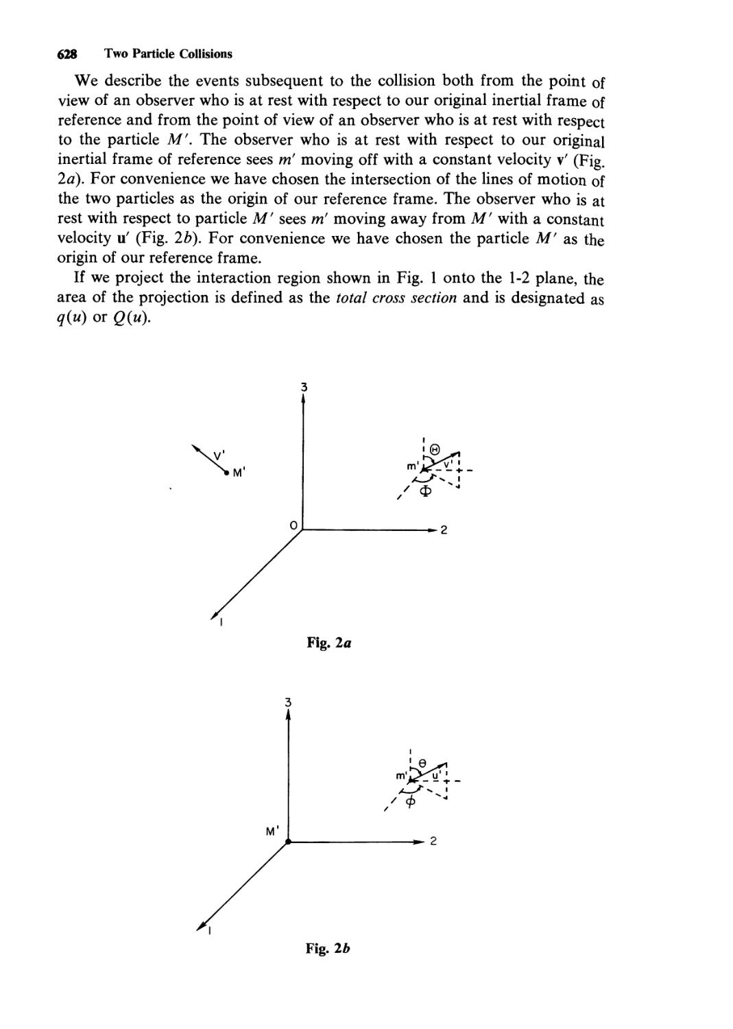


Text
CLASSICAL MECHANICS
Volume 2
EDWARD A. DESLOGE
Department of Physics
Florida State University
A WILEY-INTERSCIENCE PUBLICATION
JOHN WILEY & SONS
New York • Chichester • Brisbane • Toronto ♦ Singapore
Copyright © 1982 by John Wiley & Sons, Inc.
All rights reserved. Published simultaneously in Canada.
Reproduction or translation of any part of this work
beyond that permitted by Section 107 or 108 of the
1976 United States Copyright Act without the permission
of the copyright owner is unlawful. Requests for
permission or further information should be addressed to
the Permissions Department, John Wiley & Sons, Inc.
Library of Congress Cataloging in Publication Data:
Desloge, Edward A., 1926-
Classical mechanics.
"A Wiley-Interscience publication."
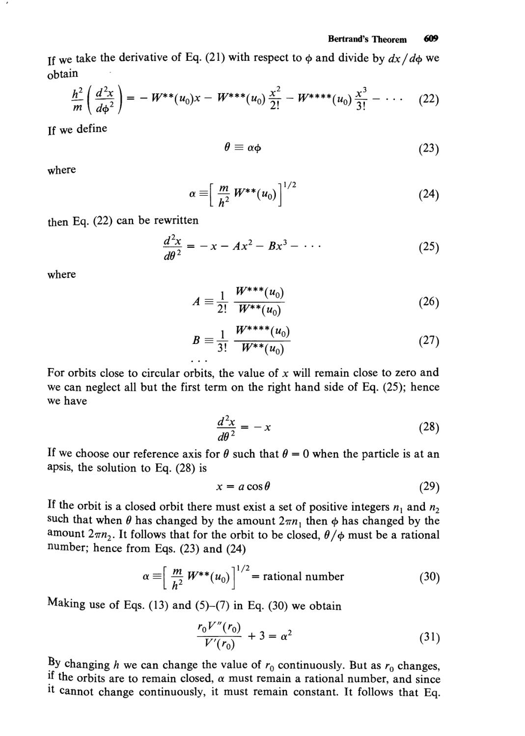
Includes index.
1. Mechanics. I. Title.
QC122.D47 531 81-11402
ISBN 0-471-09144-8 (v. 1)AACR2
ISBN 0-471-09145-6 (v. 2)
Printed in the United States of America
10 987654321
Preface
This book is the product of teaching classical mechanics on both the
undergraduate and the graduate levels intermittently over the past 20 years. It
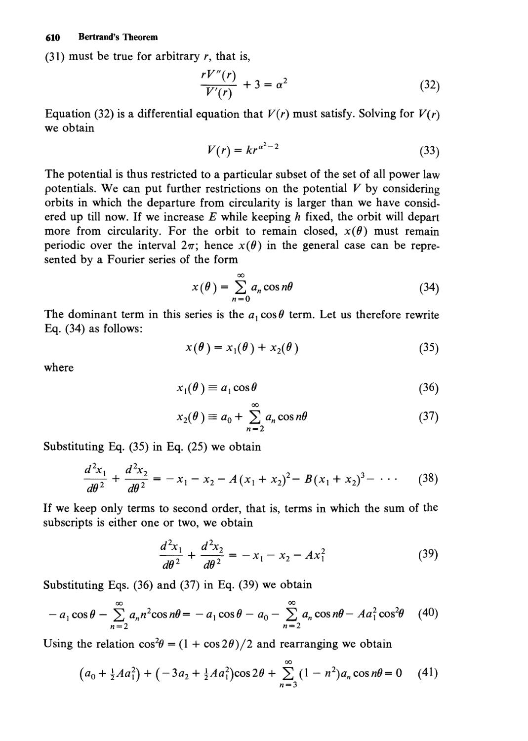
covers mechanics in a unified fashion from the foundations, through
elementary and intermediate mechanics, to a moderately advanced graduate level. A
knowledge of calculus is presumed. Any other mathematics needed is
provided in the appendices.
Volume 1 can be used as a text for an undergraduate course. Volume 2 can
be used as a text for a graduate course. By judicious deletion of material,
courses of almost any length can be accommodated. The breadth and detail of
the coverage is such that the book can also be used by students wanting to
learn mechanics on their own, or by instructors wanting to direct students
through self-paced programs. All the topics customarily found in an
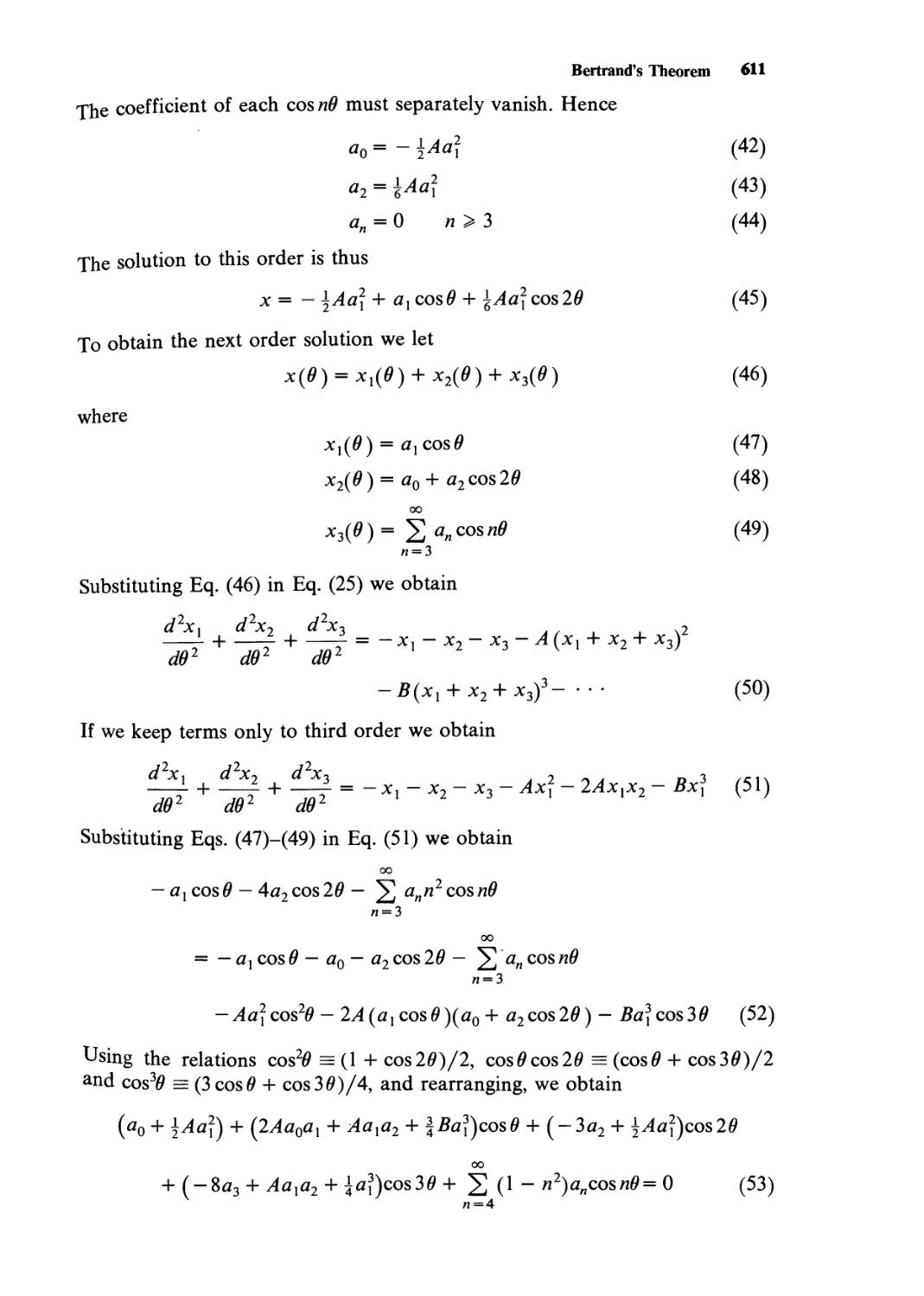
undergraduate or graduate text are covered, though frequently, in greater depth or
detail, or from a slightly different point of view. In addition there are many
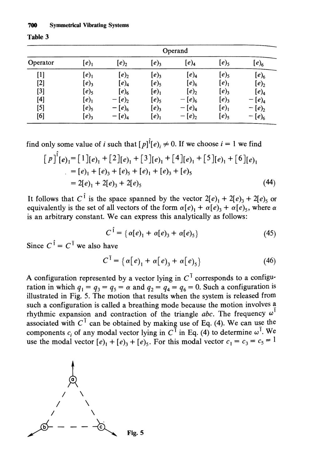
interesting and useful topics that are seldom found in the standard texts.
Hence this book can also serve as a source book for an instructor in
mechanics, or as an aid to a researcher whose need for mechanics exceeds
what is provided by the usual text.
Much material is covered, but no attempt has been made to write an
encyclopedic text on classical mechanics; rather, the subject is arranged in
such a way that additional material can be inserted easily and naturally.
A knowledge of mechanics that will continue to mature beyond the
termination of a formal course requires a clear and accurate grasp of the organization
of the subject. Throughout this book, I have tried to stress organization,
clarity, and accuracy. This emphasis may sometimes appear to result in an
approach that is overly stiff, detailed, and formal. The niceties of charm,
elegance, and warmth, where lacking, can be supplied by a good instructor. A
weakness in organization is almost impossible to repair.
One of the most crucial stages in the exposition of any subject in physics is
the choice of notation. A good notation is comprehensive; that is, it carries all
the information that is required to avoid misinterpretation, and yet it is simple.
Preface
Slight differences are often quite significant. For example it is both more
meaningful and more useful to express the components of a vector A with
respect to a frame S' as Ar rather than A-. I have thought a great deal about
the notation. If I have erred, it is more often than not in using notation that is
somewhat overloaded. The appearance of many of the discussions and
derivations could be improved by stripping the notation of some of its appendages.
The loss however would generally outweigh the gain. For example, the
appearance of arguments involving partial derivatives, such as (3// 3x)y or
equivalently df(x, y)/dy could be improved by writing such terms simply
3//3.x. I have at times done this myself. However, anyone who has taught a
course in thermodynamics will verify that the consequences can be disastrous,
if one is not careful.
In writing this book, I have used a number of organizational and
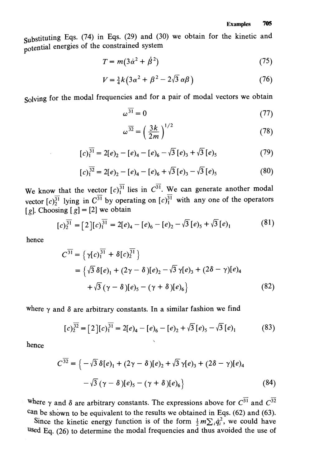
pedagogical devices that I have found over the years to be particularly helpful. (1) The
material is highly subdivided, to give emphasis to the organization and to
facilitate reorganization. (2) The chapters are short, to make assimilation easier
and to aid in the addition, deletion, or rearrangement of material. (3) Formal
definitions, postulates, and theorems are frequently used, to emphasize and
clarify important concepts and to foster exactness. (4) Most chapters contain
one or more examples designed to illustrate an idea, or to provide general
techniques for the solution of problems, rather than to serve as models to be
slavishly imitated. (5) There are a large number of problems, since the ability to
systematically solve a wide variety of problems is one of the goals of a course
in mechanics. (6) All mathematical developments needed are provided in
appendices. In this way the continuity of a physical argument is not broken, and yet
the mathematical tools are readily available.
A number of benefits, other than problem solving, can be derived from a
course in classical mechanics. Three in particular have influenced me strongly
in writing this book.
1. Since physics as we know it today had its origins in classical mechanics,
the very structure and language of physics is permeated by ideas that
come from classical mechanics; hence a knowledge of the foundations of
mechanics can provide a student with a deeper grasp of all of physics. I have
therefore devoted considerable effort to developing the foundations of
classical mechanics.
2. A course in classical mechanics is not only a course in physics but a course in
applied mathematics. The inclusion of certain topics, and the extensive
mathematical appendices in this book, reflect this aspect of mechanics. As
much consideration has been given to the writing of the appendices as to
the text proper. Though relegated to appendices, the mathematical topics
are an integral part of the text.
3. The human brain contains two hemispheres whose characters have been
shown to be different but complementary. In most individuals, the right
Preface vii
hemisphere, which is associated directly with the left hand, the left field of
vision, and so forth, is superior in handling geometrical concepts, and the
left hemisphere, which is associated directly with the right hand, the right
field of vision, and so forth, is superior in handling formal analytical
concepts. Learning physics involves an interesting interplay between these
two abilities. The left hemisphere provides the analytical map that takes us
from one point to another, while the right hemisphere provides the
geometrical vision necessary to see the goal and landmarks along the way.
A course in classical mechanics offers a marvelous vehicle for developing and
integrating both the geometrical and the analytical powers of the brain. The
Newtonian approach to mechanics is strongly geometrical, whereas the
Lagrangian and Hamiltonian approaches are strongly analytical. It
follows that a course designed to exercise both sides of the brain should, as
this text does, include a thorough foundation in Newtonian mechanics
before proceeding to Lagrangian and Hamiltonian mechanics. Too many
modern courses in classical mechanics are built on a weak foundation of
Newtonian mechanics, with the resultant complaint by instructors that a
particular student is good at mathematics but does not seem to have any
physical intuition.
To make Volume 1 adequate for an undergraduate course and Volume 2
adequate for a graduate course, certain topics are covered in both volumes.
Central force motion, the differential scattering cross section, and small
oscillations are introduced in Volume 1, and reviewed and extended in
Volume 2. Rigid body motion is covered in great detail from the Newtonian
point of view in Volume 1, and briefly reviewed and treated from the
Lagrangian point of view in Volume 2. An introduction to Lagrangian and
Hamiltonian mechanics is given in Volume 1, to prepare the student for the
full treatment in Volume 2.
To conclude this preface, I point out some aspects of the book that are
unique or are, in my opinion, treated better or more thoroughly here than
elsewhere.
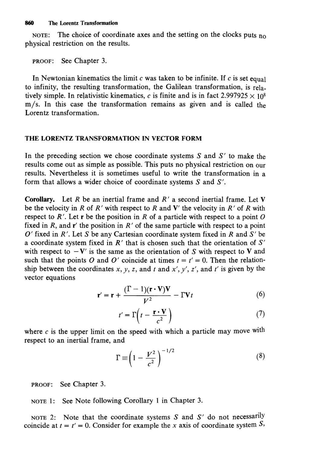
In Chapters 1-4, 85, and 86 the basic principles of Newtonian and
relativistic kinematics are derived starting from the assumption of the existence and
equivalence of inertial frames of reference. With this assumption, the law of
transformation between inertial frames arises naturally and contains only one
undetermined parameter, which is identified as the upper speed with which a
particle can move with respect to an inertial frame. By choosing this
parameter to be infinite we obtain the Galilean transformation, and by choosing it to
be finite we obtain the Lorentz transformation.
In Chapters 8, 9, 88, and 89 an investigation of quantities that might be
conserved in a collision leads naturally to the momentum conservation laws of
Newtonian and relativistic mechanics, and from these laws to the definitions
of force in both Newtonian and relativistic mechanics.
viii Preface
The treatment of the foundations of Newtonian and relativistic mechanics
contained in the two above-mentioned sets of chapters clearly brings out the
close relation between Newtonian and relativistic mechanics, and the primacy
of the law of conservation of momentum over Newton's equation of motion
and its counterpart in relativistic mechanics. It is the most thorough treatment
that can be found anywhere. Many of the details are new and unique.
Chapter 6 presents very carefully and thoroughly the definition and
properties of the angular velocity of one coordinate system with respect to another.
By starting with the analytical definition of angular velocity rather than the
geometrical definition, as is customarily done, many of the difficulties
associated with this concept are avoided. Even though a good grasp of this
concept is a prerequisite to an ability to express the laws of motion in rotating
frames, and to an understanding of the kinematics and dynamics of rigid
bodies, it is amazing to me how many of the standard texts are weak on this
subject, and frequently contain spurious definitions of angular velocity.
Chapter 23 contains one of the simplest and most organized treatments of
central force motion of which I am aware.
Chapters 24, 26, 60, and 61 contain a very complete treatment of the
differential scattering cross section. Chapter 61 derives the relationship
between the center of mass and laboratory cross sections for a collision in which
both particles are moving, the collision is inelastic, and the product particles
differ from the incident particles. No other text that I know of contains this
complete result.
The treatment of rigid body motion in Chapters 34-40, with the possible
addition of Chapters 41, 63, and 64, is sufficiently complete and detailed to
form a course by itself. Chapter 38 is a thorough treatment of the inertia
tensor from both the analytical and the geometric points of view. Chapter 39
contains an extremely detailed treatment of Euler angles, and the kinematics
of rigid body motion. The expression in Chapter 39 of the equations of
transformation between different reference frames and the relative angular
velocities between these frames in terms of Euler angles is a very useful aid to
anyone interested in solving rigid body motion problems.
Chapters 47-54 give a thorough treatment of Lagrange's equations of
motion and include a detailed treatment of constraints both holonomic and
anholonomic. Since most undergraduate courses do not have the time for such
a complete treatment, an introductory abbreviated treatment appears in
Chapters 42-44.
The treatment of small vibrations in Chapters 45 and 65 contains a number
of results that cannot be found elsewhere.
The material in Chapter 66 together with the material in Appendices 28-30
represents a complete introduction to group theory and its application to
symmetrical vibrating systems. Although the complexity of the notation makes
the going a little tedious at times, the text contains none of the gaps and
guesswork that seem to mar the treatments I have found elsewhere.
Preface ix
Quasi-coordinates and the Gibbs-Appell equations of motion covered in
Chapters 67-70 are probably unknown to most physicists. There are only a
few mechanics books in which they are even mentioned. Because I think they
deserve more attention and are quite useful in solving certain problems, I have
included them.
The treatment of Hamilton's equations of motion, canonical
transformations, and Hamilton-Jacobi theory in Chapters 71-78 is quite unusual in that
no use is made of the calculus of variations. Although this results in many of
the proofs being a little longer than usual, I feel that it provides a more secure
foundation in the subject, since most students who are encountering this
subject for the first time are not completely sure of themselves in the use of the
calculus of variations. This unsureness is usually compounded by the casual
and sometimes erroneous use of the calculus of variations by some authors.
Although I prefer not to use the calculus of variations in a student's first
encounter with Hamiltonian mechanics, I certainly believe it to be an
extremely useful tool, hence have devoted Part 8 and Appendix 32 to this
subject. The initial separation of the calculus of variations from Hamiltonian
mechanics has the added organizational advantage of allowing the instructor
who so desires to pursue the subject beyond and apart from what is required
in Hamiltonian mechanics.
The presentation of the foundation and basic principles of relativistic
mechanics in Part 9 is I believe one of the most logical and straightforward to
be found anywhere. Though some of the proofs are a little ponderous, the
general flow of concepts does not require an extraordinary distortion of a
student's imagination. As a consequence relativistic mechanics seems almost
inevitable.
The nature and importance of constants of the motion is stressed time and
again throughout the text, starting with Chapter 17 and proceeding through
Chapters 33, 46, 56, 71, and 81. Chapter 56 considers in detail the relationship
between constants of the motion and the invariance of the Lagrangian under
certain transformations, and Noether's theorem is presented without making
use of variational techniques as is usually done in those few sources where this
theorem can be found.
The subject of impulse, which usually causes students a great deal of
unnecessary grief, is developed in detail in Chapters 18, 41, and 57.
Many of the appendices are quite useful in themselves, apart from their
value in the body of the text. However since this book is intended primarily as
a mechanics text, and only secondarily as a course in applied mathematics,
many theorems in the appendices are stated without proof. Proofs that are
particularly pertinent or cannot easily be found elsewhere are given.
In Appendices 4-6, and 23, the reader is led systematically from the
geometric concept of a vector as a directed line segment to the highly
analytical concept of general tensors. With a little amplification and
completion of proofs, the material would make a good course in vectors and tensors.
x Preface
Similarly the material in Appendices 12 and 24-26, with the possible
addition of the material on quadratic forms in Appendix 27, forms a good
outline for a course in matrices.
Appendix 32 provides an excellent introduction to the calculus of
variations.
Appendices 11, 15, 19, and 22 cover a number of topics very important to
classical mechanics in a manner that is both simpler and clearer than can be
found elsewhere.
While writing this book I have not had in mind a hypothetical audience, but
rather have written as if I were to be the reader. The book is in a sense a
reflection of myself. Its exposure to numerous students over the years has
sharpened rather than altered this reflection. I suspect that this is how most
texts are written. Interestingly, I am dominantly a right hemisphere thinker—
that is, I think in terms of pictures—but the first impression one gains of the
text is that it is dominantly analytical. The probable explanation of this
apparent anomaly is that one tends to emphasize the things that are personally
difficult while at the same time ignoring what comes easily, with the result that
the material is more analogous to a photographic negative than to a positive
print. In any case the success of this book will depend on how many others
share the difficulties, problems, loves, and hates that I experienced in learning
classical mechanics. I hope that there are many, and that through this book
they will derive some of the pleasures I have found in my encounter with
classical mechanics.
Edward A. Desloge
Tallahassee, Florida
December 1981
Contents
VOLUME 1
Introduction
PART 1. THE NEWTONIAN MECHANICS OF PARTICLES
Section 1. The Basic Principles of Newtonian Kinematics
1. Space and Time, 7
2. Inertial Frames, 11
3. Transformation Between Inertial Frames, 13
4. Absolute Space and Time, 4
Section 2. Auxiliary Principles of Newtonian Kinematics
5. Relative Motion of Particles, 27
6. Relative Motion of Frames of Reference, 32
7. The Description of Motion Using Orthogonal
Curvilinear Coordinates, 43
Section 3. The Basic Principles of Newtonian Dynamics
8. Mass and Momentum, 49
9. Force, 59
10. Center of Mass, 65
Section 4. Elementary Applications of Newton's Law
11. Some Basic Forces, 73
12. Statics of a Particle, 83
13. Dynamics Problems, 88
25
47
71
Contents
Section 5. Auxiliary Principles of Newtonian Dynamics
14. Torque and Angular Momentum, 101
15. Work and Kinetic Energy, 107
16. Potential Energy, 113
17. Constants of the Motion, 120
18. Impulse, 126
19. The Equations of Motion in Noninertial
Reference Frames, 136
20. The Equations of Motion in Orthogonal
Curvilinear Coordinate Systems, 144
99
Section 6. Applications
21. One Dimensional Motion in an Arbitrary
Potential, 151
22. The Harmonic Oscillator, 158
23. Central Force Motion, 172
24. The Differential Scattering Cross Section, 187
25. Two Particle Systems, 196
26. Two Particle Collisions, 203
149
PART 2. THE NEWTONIAN MECHANICS OF SYSTEMS
OF PARTICLES
Section 1. Basic Principles
27. Dynamical Systems, 215
28. Force and Linear Momentum, 218
29. Torque and Angular Momentum, 226
30. Work and Kinetic Energy, 234
31. Cartesian Configuration Space, 240
32. Potential Energy, 243
33. Constants of the Motion, 247
213
Section 2. Rigid Body Motion
34. Rigid Bodies, 253
35. Equivalent Systems of Forces, 255
36. Statics of a Rigid Body, 264
37. Uniplanar Motion of a Rigid Body, 269
38. The Inertia Tensor, 286
251
Contents xiii
39. Rigid Body Kinematics, 303
40. Rigid Body Dynamics, 320
41. Impulsive Motion of a Rigid Body, 338
PART 3. AN INTRODUCTION TO LAGRANGIAN AND
HAMILTONIAN MECHANICS
Section 1. Lagrangian Mechanics
42. Holonomic Constraint Forces, 349
43. Generalized Coordinates for Holonomic
Systems, 352
44. Lagrange's Equations of Motion for a
Holonomic System, 361
347
Section 2. Applications of Lagrangian Mechanics
45. Vibrating Systems, 373
371
Section 3. Hamiltonian Mechanics
46. Hamilton's Equations of Motion, 387
385
SUPPLEMENTARY MATERIAL
Appendices
1. Analytical Representation of a Sine Function, 397
2. Partial Differentiation, 398
3. Jacobians, 401
4. Vector Algebra, 402
5. Vector Calculus, 408
6. Cartesian Tensors, 417
7. Orthogonal Curvilinear Coordinates, 427
8. Ordinary Differential Equations, 432
9. Linear Differential Equations, 436
10. Differentiation of an Integral, 441
11. Exact Differentials, 442
12. Matrices, 447
13. Systems of Linear Equations, 458
14. Functional Dependence, 460
15. The Method of Lagrange Multipliers, 464
16. Elliptic Functions, 467
17. Coordinate Transformations, 470
395
xiv Contents
Tables 475
1. Abbreviations of Units, 477
2. Constants, 477
3. Conversion Factors, 478
4. Centers of Mass, 479
5. Moments of Inertia, 482
6. Vector Identities, 486
Answers 489
Combined Index 1-1
VOLUME 2
PART 4. LAGRANGIAN MECHANICS
Section 1.
47.
48.
49.
50.
52.
53.
54.
55.
Lagrange's Equations of Motion
Generalized Coordinates, 513
Lagrange's Equations of Motion for Elementary
Systems, 521
Constraint Forces, 528
Lagrange's Equations of Motion for
Holonomic Systems, 538
The Determination of Holonomic
Constraint Forces, 549
Lagrange's Equations of Motion
for Anholonomic Systems, 554
Generalized Force Functions, 558
Lagrange's Equations of Motion for
Lagrangian Systems, 564
Lagrange's Equations of Motion and
Tensor Analysis, 570
511
Section 2. Auxiliary Principles of Lagrangian Mechanics
56. Constants of the Motion in the Lagrangian
Formulation, 575
57. Lagrange's Equations of Motion for
Impulsive Forces, 588
573
PART 5. APPLICATIONS OF LAGRANGIAN MECHANICS
Section 1. Central Force Motion
58. Central Force Motion, 597
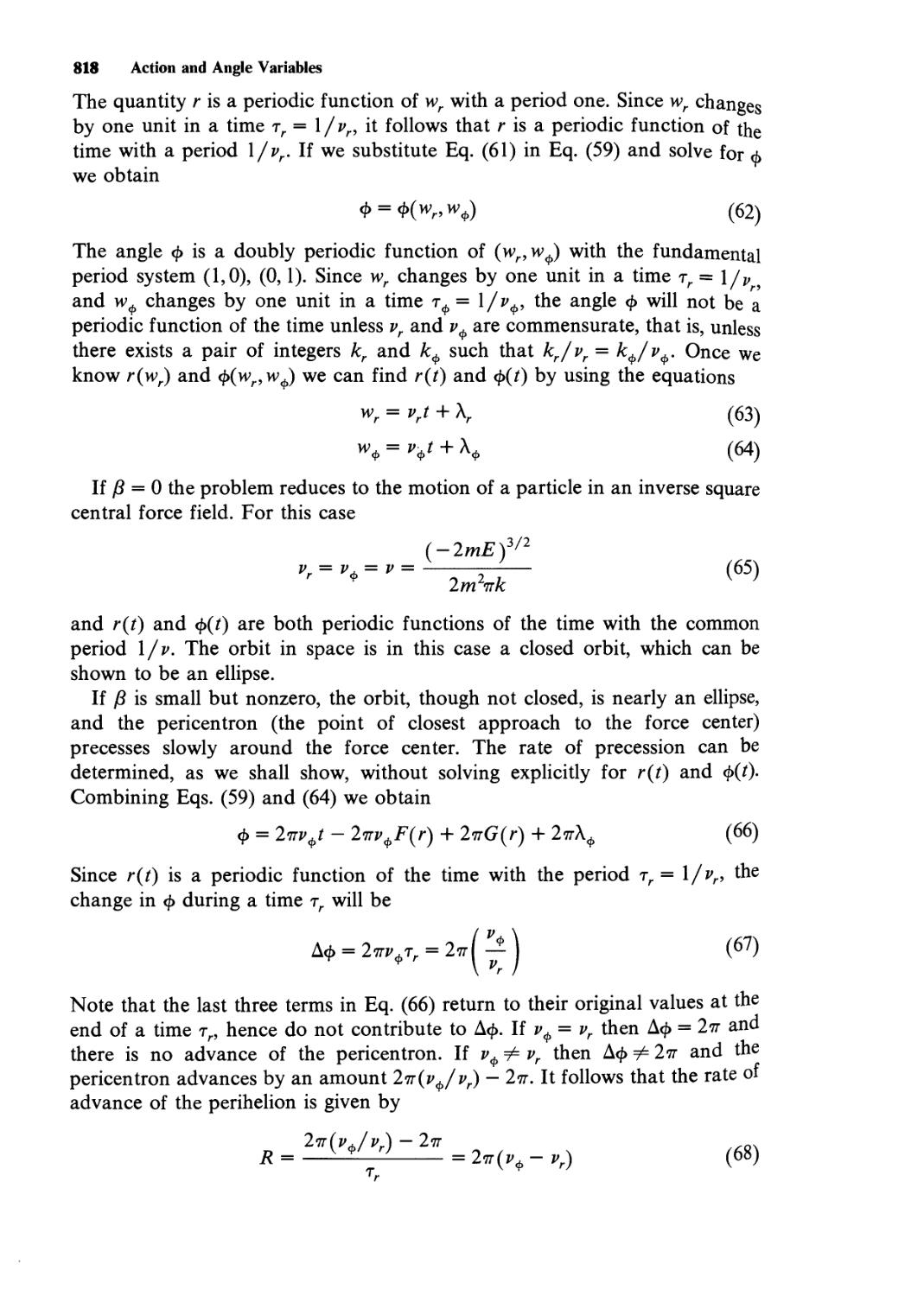
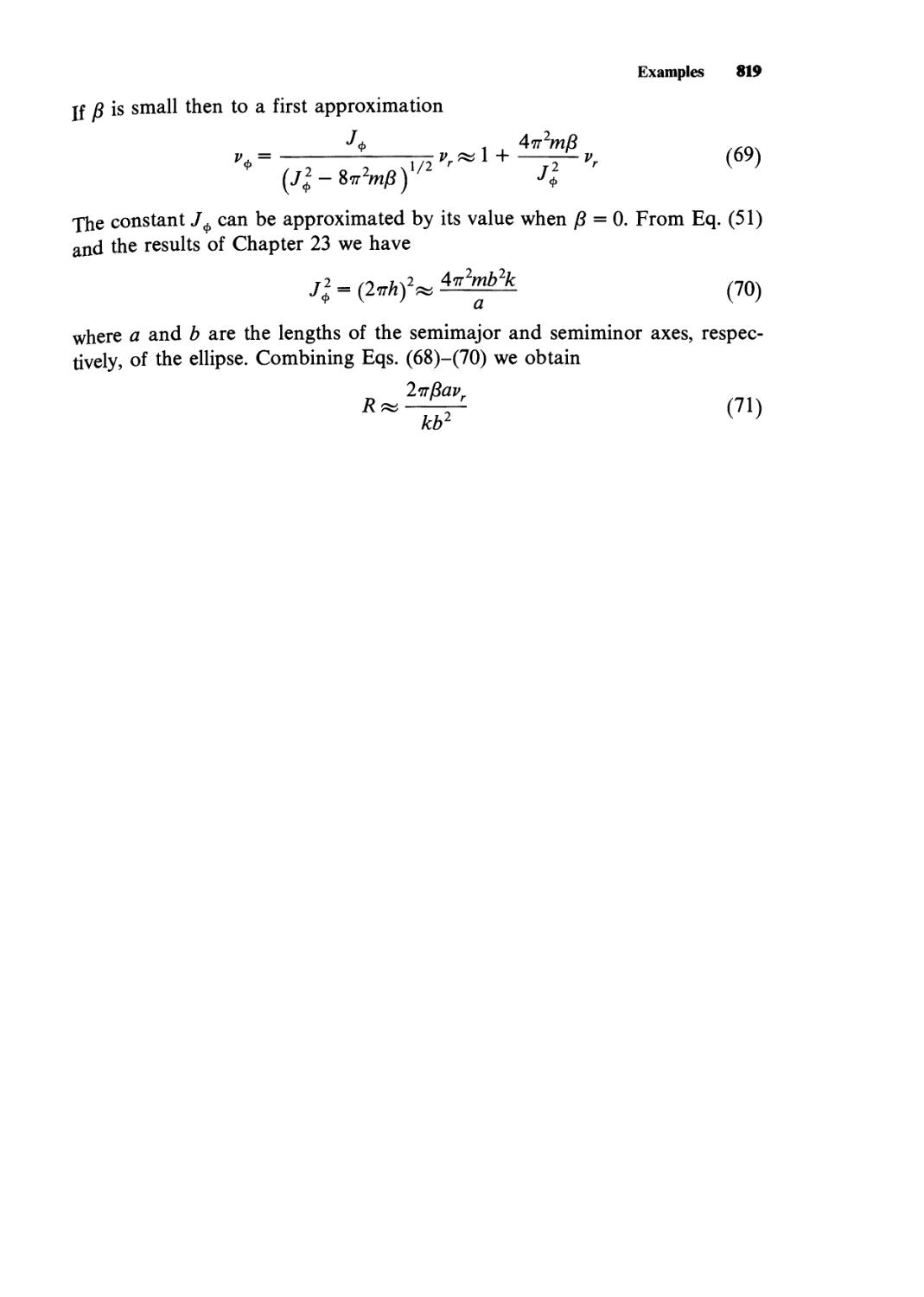
59. Bertrand's Theorem, 606
60. The Differential Scattering Cross Section, 614
61. Two Particle Collisions, 622
62. The Restricted Three Body Problem, 634
595
xvi
Section 2. Rigid Body Motion
63. Rigid Body Kinematics, 647
64. Rigid Body Dynamics, 653
Section 3. Small Oscillations
65. Vibrating Systems, 665
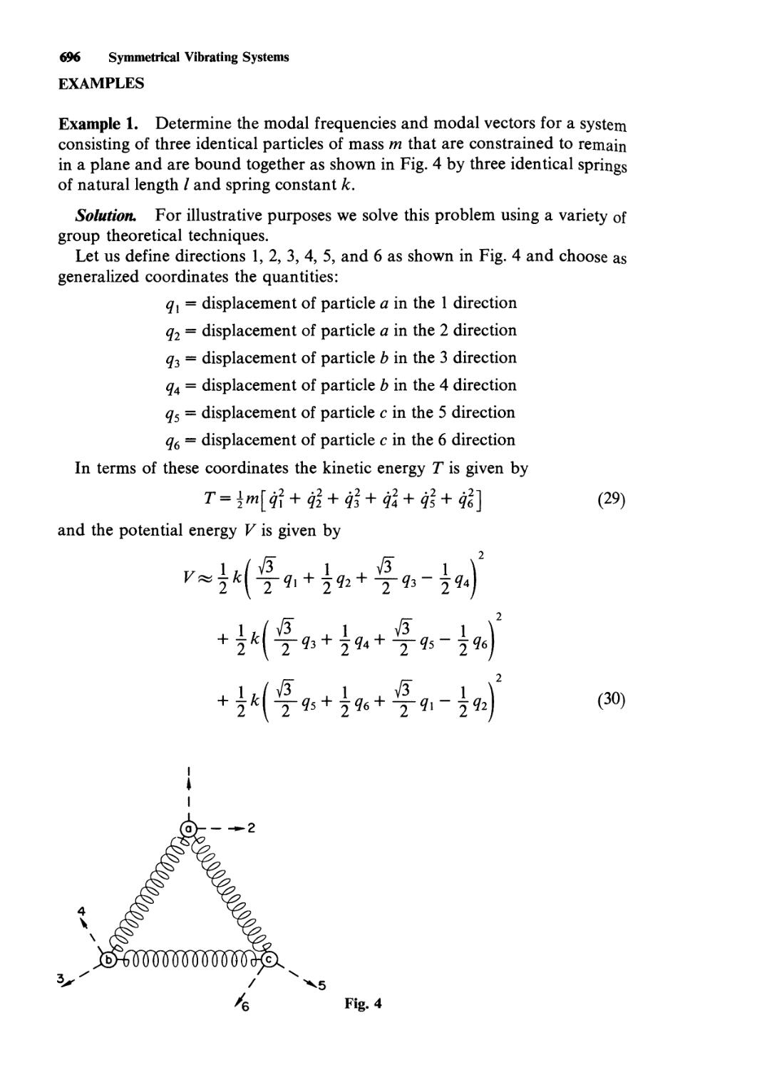
66. Symmetrical Vibrating Systems, 682
645
663
PART 6.
67.
68.
69.
70.
QUASI-COORDINATES
Quasi-Coordinates, 711
Lagrange's Equations for Quasi-Coordinates, 715
The Gibbs-Appell Equations of Motion, 720
The Gibbs-Appell Equations and Rigid
Body Motion, 727
PART 7. HAMILTONIAN MECHANICS
Section 1. Hamilton's Equations of Motion 735
71. Hamilton's Equations of Motion, 737
72. Equations of Motion of the Hamiltonian Type, 744
73. Point Transformations, 750
Section 2. Canonical Transformations 753
74. Canonical Transformations, 755
75. A Condensed Notation, 768
76. Hamilton's Canonical Equations of Motion, 773
Section 3. Hamilton-Jacobi Theory 787
77. Generating Functions, 789
78. The Hamilton-Jacobi Equations, 797
79. Action and Angle Variables, 807
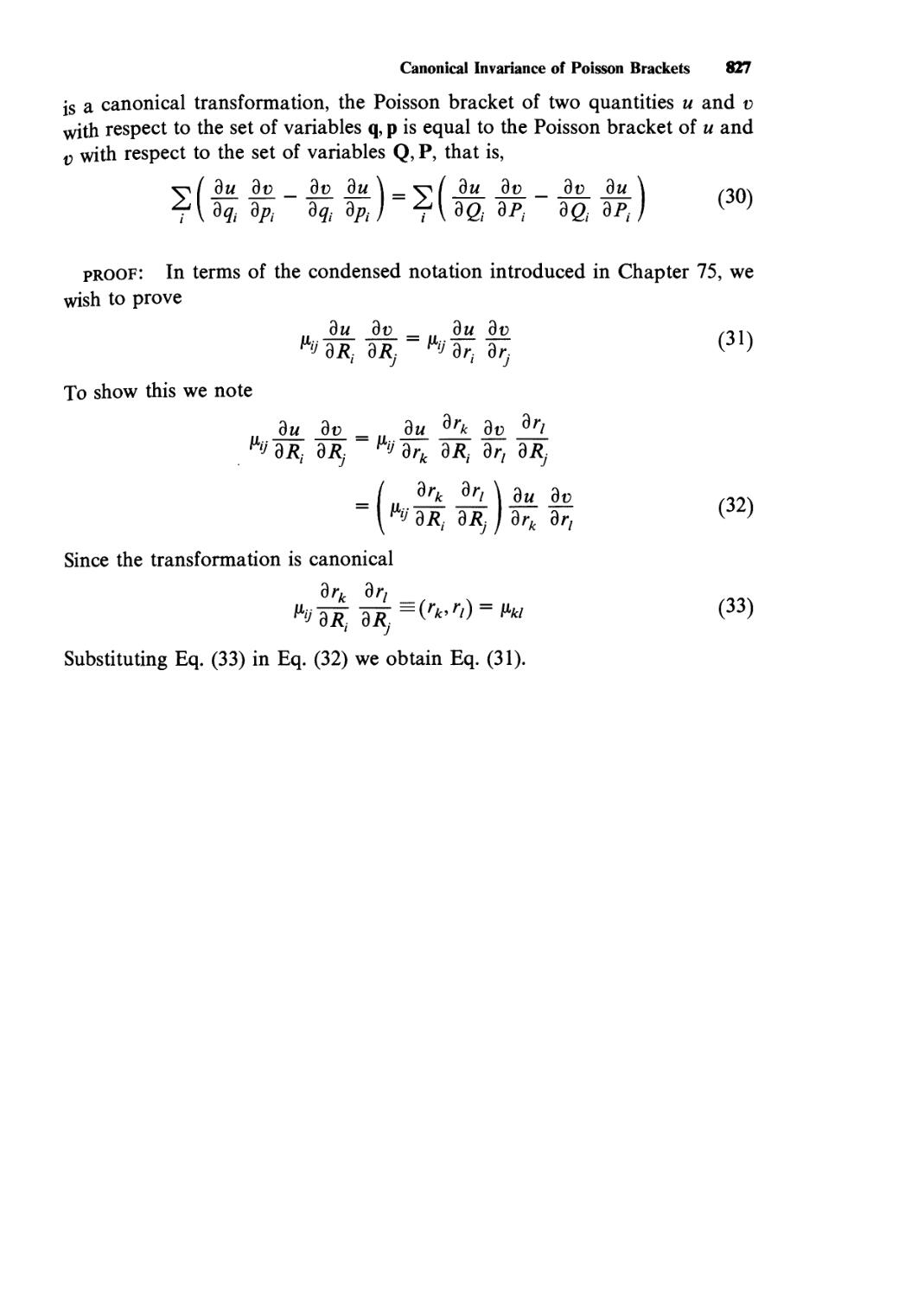
Section 4. Poisson Formulation of the Equations of Motion 821
80. Poisson Brackets, 823
81. The Poisson Formulation of the Equations
of Motion, 828
Contents xvii
PART 8. VARIATIONAL PRINCIPLES IN CLASSICAL
MECHANICS
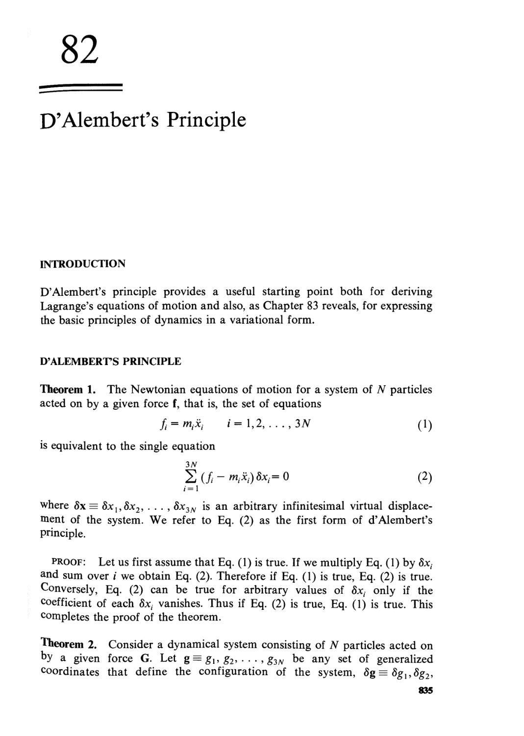
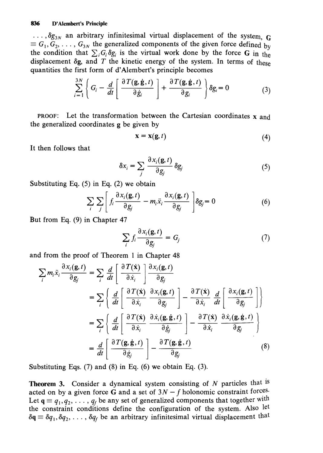
82. D'Alembert's Principle, 835
83. Hamilton's Principle, 838
84. The Modified Hamilton's Principle, 843
PART 9. RELATIVISTIC MECHANICS
Section 1. Relativistic Kinematics
85. The Basic Postulates of Relativistic Kinematics, 857
86. The Lorentz Transformation, 859
87. Some Consequences of the Lorentz
Transformation, 867
855
Section 2. Relativistic Dynamics of a Particle 873
88. Mass and Momentum, 875
89. Force, 885
90. Work and Energy, 888
Section 3. Four Dimensional Formulation of Relativistic
Mechanics 891
91. Four Dimensional Formulation of Relativistic
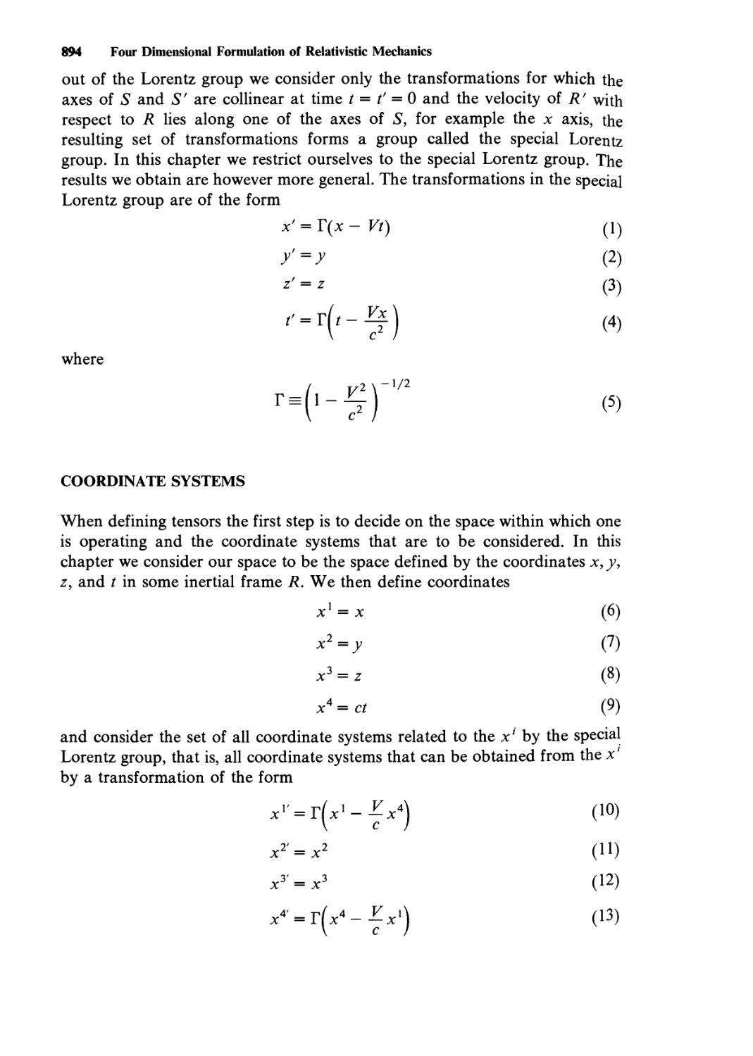
Mechanics, 893
Section 4. Relativistic Lagrangian and Hainiltonian Mechanics 899
92. Relativistic Lagrangian Mechanics, 901
93. Relativistic Hamiltonian Mechanics, 903
SUPPLEMENTARY MATERIAL
Appendices
18. Inverse Transformations, 909
19. Change of Variables in an Integral, 912
20. Euler's Theorem, 914
21. The Gram-Schmidt Orthogonalization Process, 915
22. Legendre Transformations, 918
23. General Tensors, 921
907
xviii Contents
24. Matrix Transformations, 928
25. Eigenvalues of Matrices, 931
26. Diagonalization of Matrices, 935
27. Quadratic Forms, 937
28. Group Theory, 945
29. Vector Spaces, 951
30. Representations of a Group, 955
31. Multiply Periodic Functions, 967
32. Calculus of Variations, 968
Answers 981
Combined Index 1-1
CLASSICAL MECHANICS
Volume 2
PART
LAGRANGIAN
MECHANICS
SECTION
Lagrange's Equations
of Motion
47
Generalized Coordinates
INTRODUCTION
The material in this and the chapters that follow provides a complete and
detailed analysis of Lagrangian dynamics. There is some danger however that,
because of the detail and the generality of the results, the reader will lose sight
of the essential simplicity of the Lagrangian approach. To counteract this
danger, any reader who has not previously encountered Lagrange's equations
of motion should read the material in Chapters 42-44 in Volume 1 before
starting this section.
NEWTON'S LAW
The position of a particle can be specified by giving its coordinates Xi , Xy^ 3
with respect to a Cartesian coordinate system S fixed in an inertial frame. If
the mass of the particle is m and the components of the force acting on the
particle are/,, /2, and/3, the motion of the particle can be determined by
Newton's law
/ = mxi i = 1,2,3 (1)
The configuration of a system of N particles can be specified by the set of
coordinates jc,(1),x2(l),x3(l),x,(2), ..., where xt{n) is the /th coordinate of
the A th particle. If the mass of the nth particle is m(n) and the components of
the force acting on the nth particle are/,(«),/2(«), and/3(«), the motion of the
system can be determined by the set of equations
/,(«) = m{n)xt{n) /-1,2,3
n= 1,..., N
513
514 Generalized Coordinates
The discussion of systems of particles can be considerably simplified if we
use the notation introduced in Chapter 31, that is, if we let
Xi(n) = X3n-3 + i
fi(n)=f3n-3 + i
m(n) = m3n_2 = m3n_x = m3n (3)
With this notation, the configuration of a system of N particles can be
described by the set of coordinates x = xux2, . . . , x3N. Geometrically, the
configuration x of the system can be represented by a single point in the
Cartesian configuration space x, which is the space whose coordinates are the
members of the set of coordinates x. The motion of this point is governed by
Newton's law, which in terms of the set of coordinates x is simply
fi = mixi /=1,2, ...,37V (4)
Besides the set x there are many other sets of coordinates that could be used
to describe the configuration of the system. Thus in this Section we consider
the possibility of using sets of coordinates other than x, and we determine the
modification of the equations of motion that must be made when they are
used.
GENERALIZED COORDINATES AND VELOCITIES
Let us assume that we are given a dynamical system consisting of N particles.
If there exists a set of 37V coordinates g]9 g2, . . . , g3N that uniquely specifies
the configuration of the system, the coordinates gl9 g2, . . . , g3N are called
generalized coordinates and their time rates of change gl9 g2, . . . , g3N are
called generalized velocities. We designate the set gl9 g2, . . . , g3N as the set g,
and the set g]9 gl9 . . . , g3N as the set g. Just as we can represent the
configuration of a system by a point in the Cartesian configuration space x,
we can more generally represent the configuration of a system by a point in a
space whose coordinates are any set of generalized coordinates g. Such a space
is called simply a configuration space. The Cartesian configuration space x is
a particular example of a configuration space. We call the configuration space
whose coordinates are the set g, the configuration space g.
note: The reader who is already familiar with the use of generalized
coordinates may be disturbed by the use of the symbol g{ to represent a
generalized coordinate rather than the more conventional qr The symbol gi
was chosen to permit us initially to distinguish between the full 37V
dimensional configuration space and the reduced configuration space that is used
when holonomic systems are being considered. The letters qi are reserved for
the latter case.
Generalized Components of a Force 515
VIRTUAL DISPLACEMENTS AND VIRTUAL WORK
Generalization of the equations of motion requires not only the generalization
of what is meant by coordinates, but also generalization of what is meant by
the components of a force. Before we can carry this out, the concepts of
virtual displacement and virtual work must be introduced.
A virtual displacement of a dynamical system is a hypothetical change in the
configuration of the system at some fixed time t. The notation 8g=8gu
§g . . , 8g3N designates an infinitesimal virtual displacement.
Two points should be particularly noticed in the foregoing definition. First a
virtual displacement occurs at a particular time t and does not involve a
change in the time. We can imagine the system to be initially frozen in its
configuration at time t, at which point we step in and alter its configuration.
The second point to notice is that a virtual displacement does not in general
correspond to the actual displacement the system undergoes as a result of the
forces acting on it. It is for this reason that we use the notation Sg rather than
dg, since the quantity dg usually designates the actual displacement of the
system in a time dt.
The virtual work 8W of a force in the virtual displacement 8g is the work
that would be done by the force if the system underwent the virtual
displacement 8g.
Since a virtual displacement occurs at a fixed time t, the value of the force
that is acting on the system at the time t is used in calculating the virtual work
at time t. If the force is a velocity dependent force, the value of the velocity of
the system at the time t is used in evaluating the force.
GENERALIZED COMPONENTS OF A FORCE
With the introduction of the concept of virtual work we are in a position to
define generalized components of a force. This is done in the following
theorem.
Theorem 1. If a dynamical system consisting of N particles, whose
configuration can be defined in terms of the set of generalized coordinates g = gx,
£2* • • • , £3a/ is acted on by a force, the virtual work 8W of the force in an
arbitrary infinitesimal virtual displacement Sg can be written in the form
SW'-SG/Sft (5)
i
The quantities Gx, G2, ..., G3N are called generalized components of the force.
A particular generalized component Gt is called the gt generalized component
of the force or simply the gt component of the force. The set of generalized
components is designated G. The force whose generalized components are the
set G is called the force G.
516 Generalized Coordinates
proof: At a given time the virtual work 8W depends only on the force
and the virtual displacement Sg. If we expand 8W in powers of Sg1?
8gi> • • • > ^3n anc* note ^at tne higher order terms can be dropped because
the 8G; are infinitesimals, we obtain Eq. (5). This completes the proof.
Since Eq. (5) must be true for arbitrary infinitesimal virtual displacements
Sg, the gi component of a force can be determined by calculating the work
done in an infinitesimal displacement in which the generalized coordinate g is
varied while all the other generalized coordinates are held fixed, then dividing
the work done SW by the displacement Sg.
If we choose the set of coordinates x as our generalized coordinates, the
work done in an infinitesimal displacement is given by
«^=S/y fix, (6)
i
It follows that the x( generalized component of the force, which we designate
as X( or Gx, is just/, that is,
G^X^f,. (7)
note 1: The g component of a force does not in general have the
dimensions of a force. For example if g is an angle, the g component of the
force will have the dimensions of a torque, not a force. It follows that the g
component of a force cannot be interpreted as the component of the force in
the gi direction. The relationship between these two quantities is considered in
greater detail in a later section.
note 2: The value of the g component of a force depends not only on the
coordinate g but also on the other coordinates in the set g, in the same sense
that a partial derivative depends not only on the quantity that is varied but
also on the quantities that are held constant. It would therefore be more
precise to speak of "the g component in the space g" than of "the
g component." However for the sake of simplicity we use the shorter
terminology.
THE TRANSFORMATION OF THE GENERALIZED
COMPONENTS OF A FORCE
If we know the generalized components of a force in one space and we wish to
find the generalized components in another space we can use the following
theorem.
Theorem 2. If Gu G2, . . . , G3N are the components of a force in the space
whose coordinates are g,, g2, . . . , g3N, the components Gv, G2, ..., G3N, in
The Physical Components of a Force 517
the space whose coordinates are gr, gT, ..., g3N, are given by
proof: From Theorem 1 the Gj are defined by the condition
SW^GjSgj (9)
J
and the Gr are defined by the condition
8W=2lGr8gi, (10)
But
% = 2^> (ii)
Combining Eqs. (9)-(11) we obtain
SMfr-SSGylrte (12)
/" /' j Si'
Equating the coefficients of 8gr on both sides we obtain Eq. (8).
If we use Theorem 2 to transform generalized components in the space x to
generalized components in the space g we obtain
Gi-Zfj-ifc1 <13>
Equation (13) can be and often is used as the definition of the gi generalized
component of a force. The definition given in Theorem 1 is preferable for two
reasons: (a) it is ordinarily easier to calculate the generalized components of a
force starting with Eq. (5) in Theorem 1 than with Eq. (13); (b) using Eq. (13)
as the definition elevates the Cartesian configuration space to a special status,
which partially defeats our ultimate purpose, namely, to put all configuration
spaces on an equal footing.
THE PHYSICAL COMPONENTS OF A FORCE
If the coordinate gi undergoes an infinitesimal virtual change 8gt while the
remaining members of the set g are held fixed, the point x representing the
configuration of the system in the Cartesian configuration space will undergo
an infinitesimal virtual displacement. The direction of this displacement in the
x space is referred to as the gt direction.
518 Generalized Coordinates
If we represent a force f as a directed line segment in the space x, the
orthogonal projection of the force onto the g- direction is called the physical
component of the force in the g- direction and is designated F&. As we pointed
out in the preceding section the quantity G/5 the g- generalized component of a
force, and the quantity F&, the physical component of the force in the g-
direction, are not in general equal.
In the Cartesian space x the physical component Fx is identical with the
quantity we have been calling/, and as we have seen earlier/ is also identical
to the xt generalized component Xi9 that is,
^ = /5 = */ (14)
To determine the general relationship between F 9 the physical component
in the g- direction of a force, and Gh the g generalized component of the
force, we note first that the component in the x. direction of a virtual
displacement in the g- direction is
^ = ¾¾ (15)
hence the component in the x- direction of n(g,), the unit vector in the g,
direction, is
V&)= r-,, .- 21./2 (16)
If we take the scalar product of the unit vector n( g) with the force vector f we
obtain the physical component in the g direction of the force f, that is,
Comparing Eqs. (17) and (13) we obtain
[2/3ya&)2]
It follows that Gh the g component of the force, and F&, the physical
component of the force in the g direction, are not equal but are related as
shown above.
THE ORDINARY COMPONENTS OF A FORCE
There are still other quantities, besides the generalized components and the
physical components, that are called the components of a force. The most
common are what we shall call the ordinary components of a force. The
ordinary components in the g directions of a force are defined as the set of
g2 direction
Examples 519
■ g, direction
Fig.l
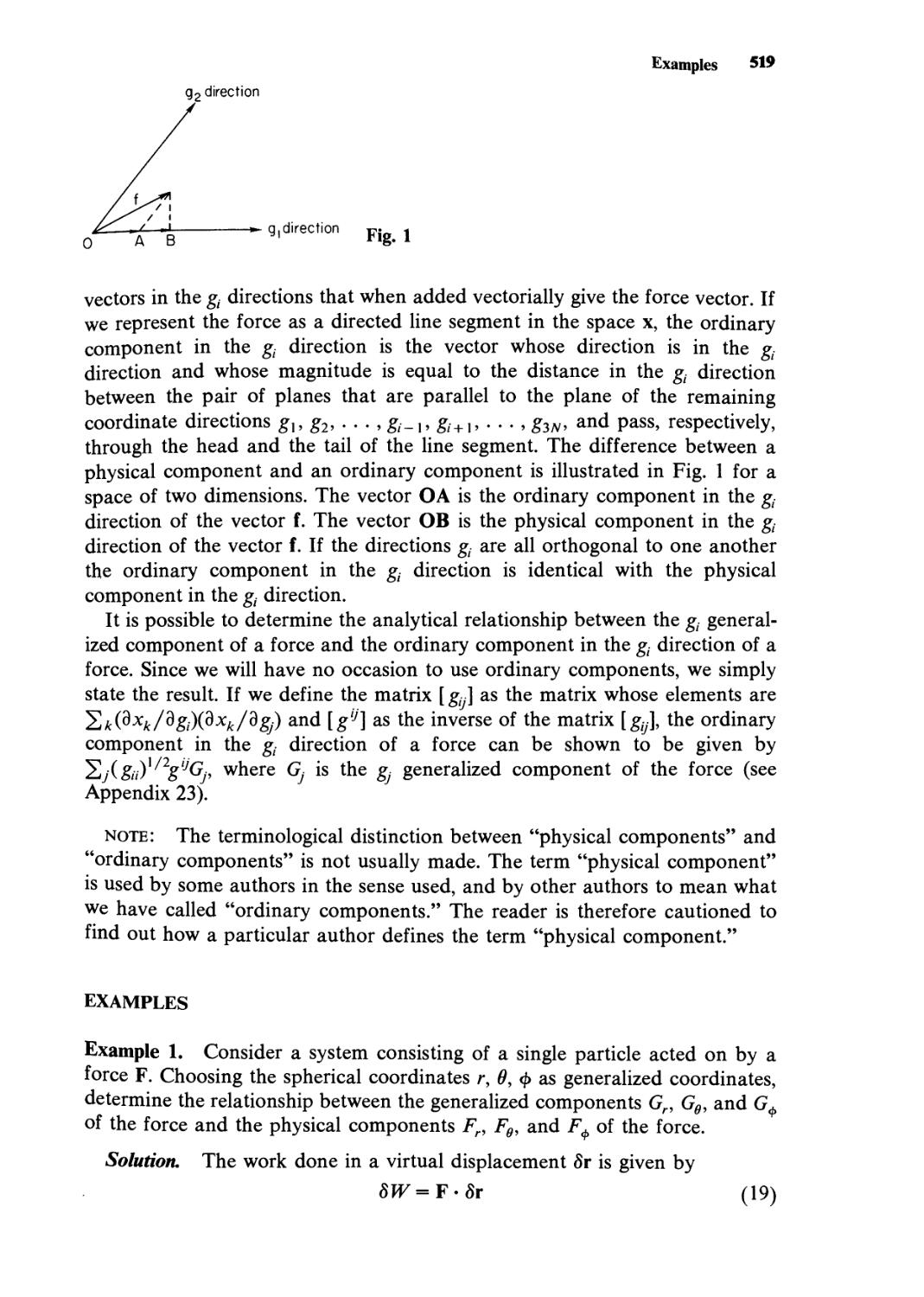
vectors in the g directions that when added vectorially give the force vector. If
we represent the force as a directed line segment in the space x, the ordinary
component in the g- direction is the vector whose direction is in the g-
direction and whose magnitude is equal to the distance in the g. direction
between the pair of planes that are parallel to the plane of the remaining
coordinate directions g,, g2, . . . , g_,, g + 1, . . . , g3yv, and pass, respectively,
through the head and the tail of the line segment. The difference between a
physical component and an ordinary component is illustrated in Fig. 1 for a
space of two dimensions. The vector OA is the ordinary component in the g-
direction of the vector f. The vector OB is the physical component in the g
direction of the vector f. If the directions g are all orthogonal to one another
the ordinary component in the g direction is identical with the physical
component in the g direction.
It is possible to determine the analytical relationship between the g
generalized component of a force and the ordinary component in the g direction of a
force. Since we will have no occasion to use ordinary components, we simply
state the result. If we define the matrix [ gy] as the matrix whose elements are
*Ek(dxk/dgi)(dXk/dgj) and [giJ] as the inverse of the matrix [gy], the ordinary
component in the g direction of a force can be shown to be given by
*2j(gn)]/2giJGp where Gj is the gj generalized component of the force (see
Appendix 23).
note: The terminological distinction between "physical components" and
"ordinary components" is not usually made. The term "physical component"
is used by some authors in the sense used, and by other authors to mean what
we have called "ordinary components." The reader is therefore cautioned to
find out how a particular author defines the term "physical component."
EXAMPLES
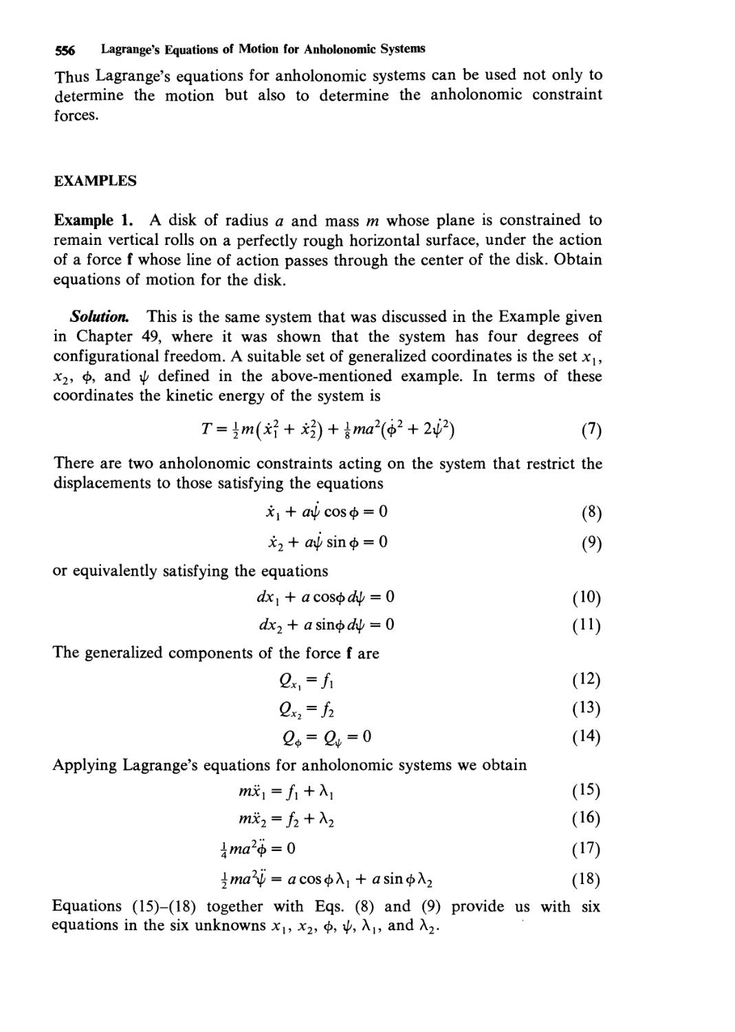
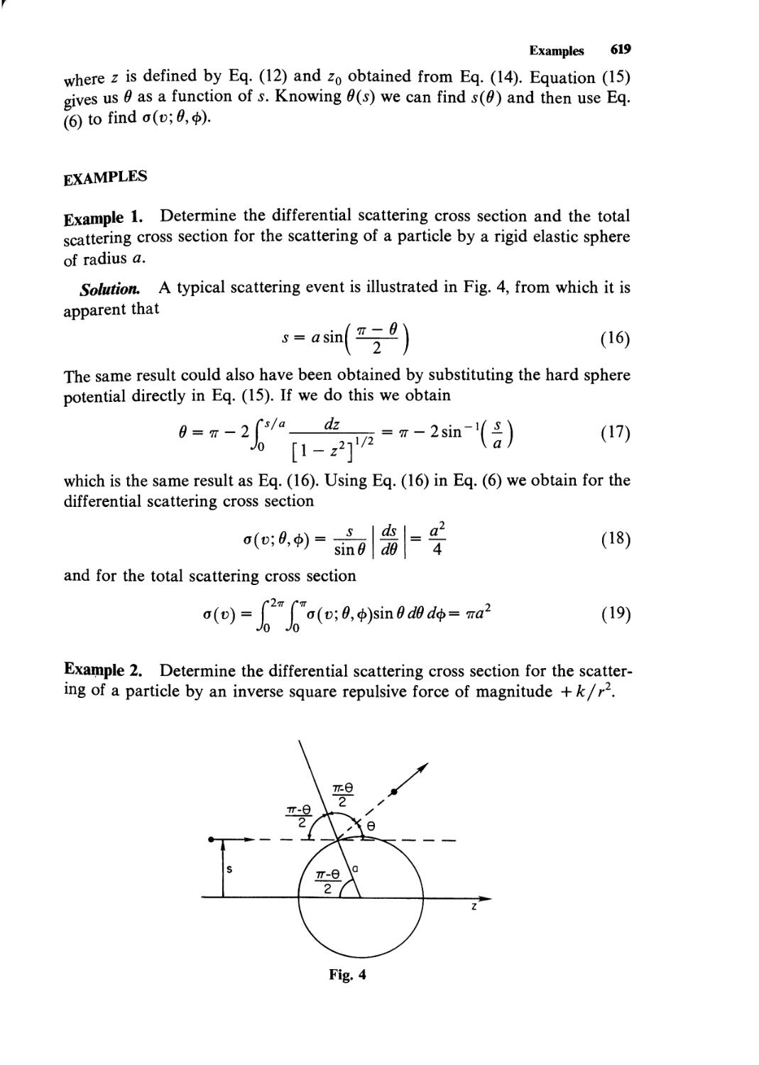
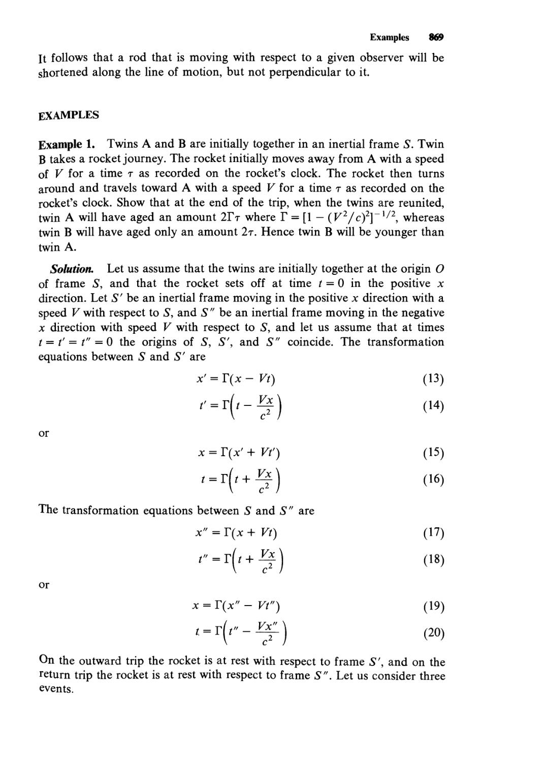
Example 1. Consider a system consisting of a single particle acted on by a
force F. Choosing the spherical coordinates r, 0, <f> as generalized coordinates,
determine the relationship between the generalized components Gn G0, and G^
of the force and the physical components Fn F0, and F^ of the force.
Solution. The work done in a virtual displacement 8r is given by
SW=F-8r (19)
520 Generalized Coordinates
Expressing F and Sr in terms of the unit vectors er, eB, and e^, we obtain
F=Frer+F9e9 + Ffy (20)
Sr = 8rer + r80e9 + rsm08<j>e^ (21)
Substituting Eqs. (20) and (21) in Eq. (19) we obtain
8W = Fr 8r + rF9 80 + r sin 0 F^8<j> (22)
From the definition of the generalized components of a force we have
8W= Gr8r + G980+ G^8<j> (23)
Comparing Eqs. (22) and (23) we obtain
Gr-F, (24)
G9 = rF9 (25)
G^rsmOFt (26)
PROBLEMS
1. A system consists of a particle of mass m suspended from a fixed point O
by a string of length a. Let r, 0, and <f> be the spherical coordinates that
determine the position of the particle with respect to the point O. Let the
polar axis be vertically down. Choosing r, 0, and § as generalized
coordinates, determine the generalized components of the gravitational
force mg and the force T that the string exerts on the particle.
2. A system consists of two particles of masses m and M, respectively, that
are in a gravitational field and interact with each other by means of a
repulsive force that is directed along the line joining the two particles and
is of magnitude/(r), where r is the distance between the two particles. Let
X, Y, Z be the Cartesian coordinates of the center of mass of the system,
and r,0,<j> the spherical coordinates that determine the position of the
particle of mass m with respect to the particle of mass M. Let the Z axis
and the polar axis be vertically up. Choosing X, Y, Z, r, 0, and § as
generalized coordinates, determine the generalized components of the
force acting on the system.
48
Lagrange's Equations of Motion for
Elementary Systems
INTRODUCTION
If a dynamical system is acted on by a set of known forces, the motion of the
system is governed by the equations f{ = m^. The aim of this chapter is to
generalize these equations, that is, to find equations of motion that are valid
for any set of coordinate g = gu g2, . . . , g3N, not just for the set of coordi-
nates x = xi,Xy9 • • • > 3n*
ELEMENTARY SYSTEMS
We use the term elementary system to mean a dynamical system containing a
known number of particles on which known forces are acting. Our interest in
this chapter is in elementary systems.
A USEFUL LEMMA
We will find the following lemma useful in the proof in the next section and in
a number of later proofs.
Lemma 1. Let g = gl, g2, . . . , g3N and g' = gv, g2., ..., g3N, be two sets of
generalized coordinates, and g = gu g2, . . . , g3N and g' = gv, g2.9 ..., g3N,
be the corresponding sets of generalized velocities. Then
3&<ft8>0 _ d
dgj dt
521
(1)
522 Lagrange's Equations of Motion for Elementary Systems
and
Hj
hj
(2)
proof: If we are given the transformation
it follows that
a?
(3)
(4)
Treating gr as a function of g, g, and t and taking the partial derivative with
respect to g- we obtain
3gK&g>0 a2g,-(g>0 . 3V(g,Q
3§ r hjh« 8k Hjtt
= 2
k
d
dt
3&
' 3&(ft0 '
[38-(8.01
.
hj \
&+i
' 3^(8.0'
9§
(5)
which is the first part of the lemma. To prove the second part we again start
with Eq. (4). Treating gr as a function of g, g, and t and taking the partial
derivative with respect to gj, we immediately obtain Eq. (2), which completes
the proof of the lemma.
LAGRANGE'S EQUATION OF MOTION FOR ELEMENTARY SYSTEMS
We are now in a position to determine the generalized equations of motion for
an elementary system. The result is stated in the following theorem.
Theorem 1. If a dynamical system consisting of TV particles is moving under
the action of a known force, the equations of motion of the system in terms of
the generalized coordinates gl5 g2, . . . , g3N are
A
dt
97Xg,g,0
*T(g,g9t)
3ft
= G,
(6)
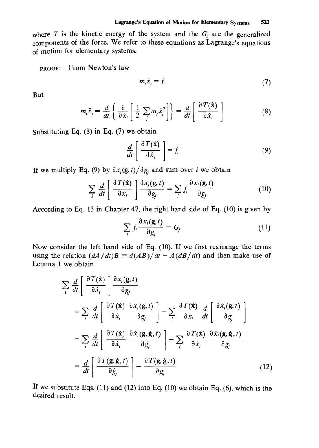
Lagrange's Equation of Motion for Elementary Systems 523
where T is the kinetic energy of the system and the G, are the generalized
components of the force. We refer to these equations as Lagrange's equations
of motion for elementary systems.
proof: From Newton's law
But
"*-i\&
"V*/=//
t2>/*/
A
dt
3T(x)
3x,
Substituting Eq. (8) in Eq. (7) we obtain
A
dt
3T(i)
= /'
If we multiply Eq. (9) by 3x,(g, t)/dg- and sum over i we obtain
dt
3T(*)
dx.
3x,(&0 = 3*,(&0
(7)
(8)
(9)
(10)
3¾ ?■" a®
According to Eq. 13 in Chapter 47, the right hand side of Eq. (10) is given by
(ii)
2/,^-*
Now consider the left hand side of Eq. (10). If we first rearrange the terms
using the relation {dA/di)B = d(AB)/dt - A{dB/dt) and then make use of
Lemma 1 we obtain
dt
= ?l
3r(x)13x,(g,Q
**i \ dSj
9T(i) 3x,(g,Q
3x, 3g;
3T(x) 3x,(g,g,Q
dX;
97X*) J
3x- J/
3*,(g,Q
= ?l
3r(&g,/)
8®
9§
3r(g,g,/)
9£
-S
3r(x) 3x,(g,g,0
3X:
9§-
(12)
If we substitute Eqs. (11) and (12) into Eq. (10) we obtain Eq. (6), which is the
desired result.
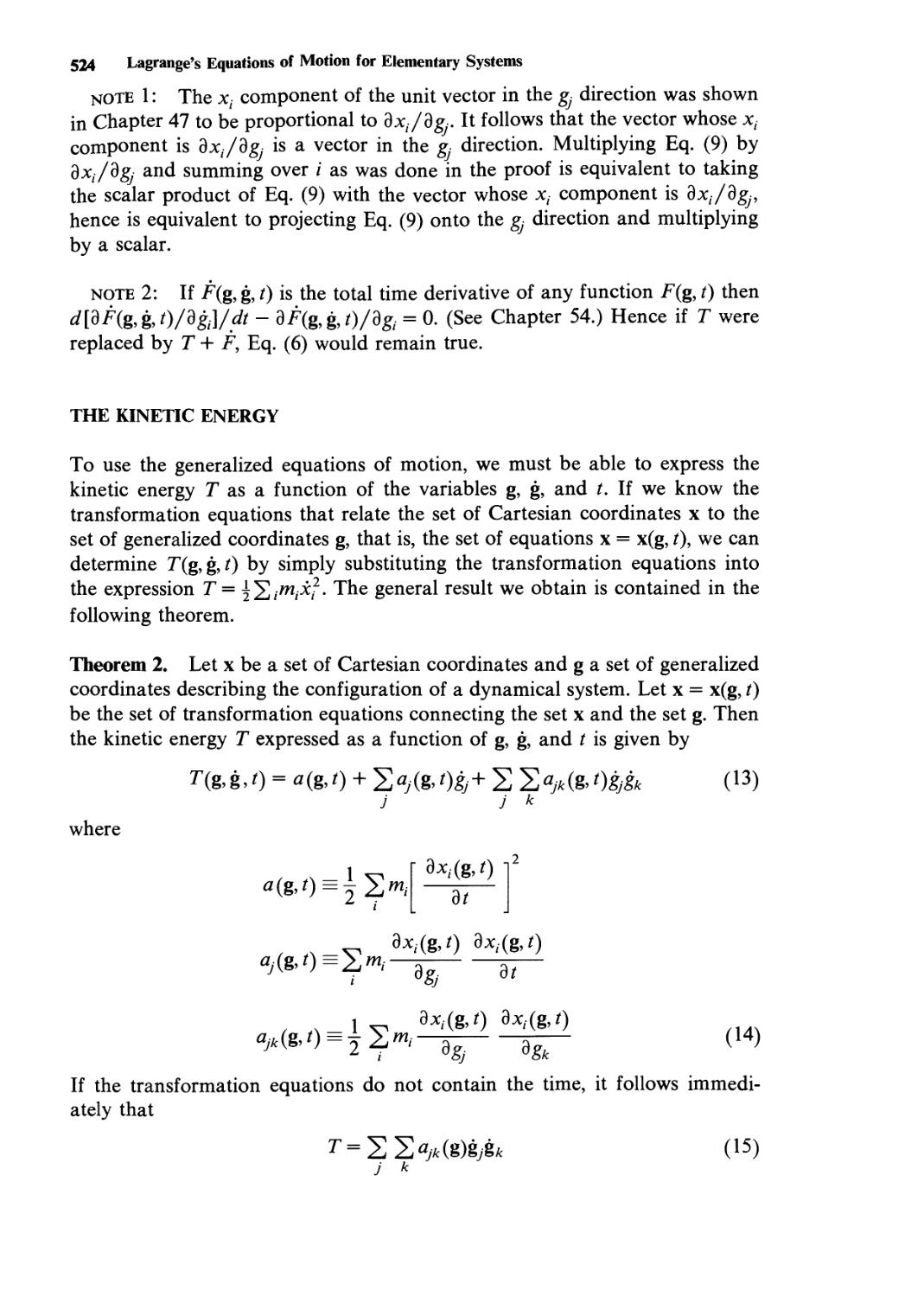
524 Lagrange's Equations of Motion for Elementary Systems
note 1: The xt component of the unit vector in the g- direction was shown
in Chapter 47 to be proportional to dx^dgj. It follows that the vector whose xt
component is dxjdgj is a vector in the g- direction. Multiplying Eq. (9) by
dxt/dgj and summing over i as was done in the proof is equivalent to taking
the scalar product of Eq. (9) with the vector whose x,- component is dx^/dgj,
hence is equivalent to projecting Eq. (9) onto the gj direction and multiplying
by a scalar.
note 2: If F(g, g, i) is the total time derivative of any function F(g, t) then
^[3^(&ft 0/3&V* - 3A&&0/3& = 0. (See Chapter 54.) Hence if T were
replaced by T + F, Eq. (6) would remain true.
THE KINETIC ENERGY
To use the generalized equations of motion, we must be able to express the
kinetic energy 77 as a function of the variables g, g, and t. If we know the
transformation equations that relate the set of Cartesian coordinates x to the
set of generalized coordinates g, that is, the set of equations x = x(g, /), we can
determine 7"(g,g, t) by simply substituting the transformation equations into
the expression T = ^^/^V^2- The general result we obtain is contained in the
following theorem.
Theorem 2. Let x be a set of Cartesian coordinates and g a set of generalized
coordinates describing the configuration of a dynamical system. Let x = x(g, t)
be the set of transformation equations connecting the set x and the set g. Then
the kinetic energy T expressed as a function of g, g, and t is given by
T(g,g,t) = a(g,t) + 2«;(&04/+ S £«;*(&')&& (13)
J J k
where
_ 1
fl(&0-o 2"1/
2
dt
2
«y(*0s2»*-a£ 97-
«,*(&') = 2 ?m'^ hT (14)
If the transformation equations do not contain the time, it follows
immediately that
r=2 2«y*(g)M* (15)
j k
Examples 525
proof: Substituting the transformation equations into the Cartesian
expression for the kinetic energy we obtain
•2
T=j^mixf
= \ 2w,
9*
+ 22
dx,(g,t) . 3x,(&9
3*,(&0
9x,(g.O . 3*,(&0
9/
3?
+ 2
J
,m,
3^(gv0 3x,(g,f)
3¾ 9/
Sj
1 ^ 3*/(&0 3*/(&0
§•&
7 J k
which completes the proof of the theorem.
(16)
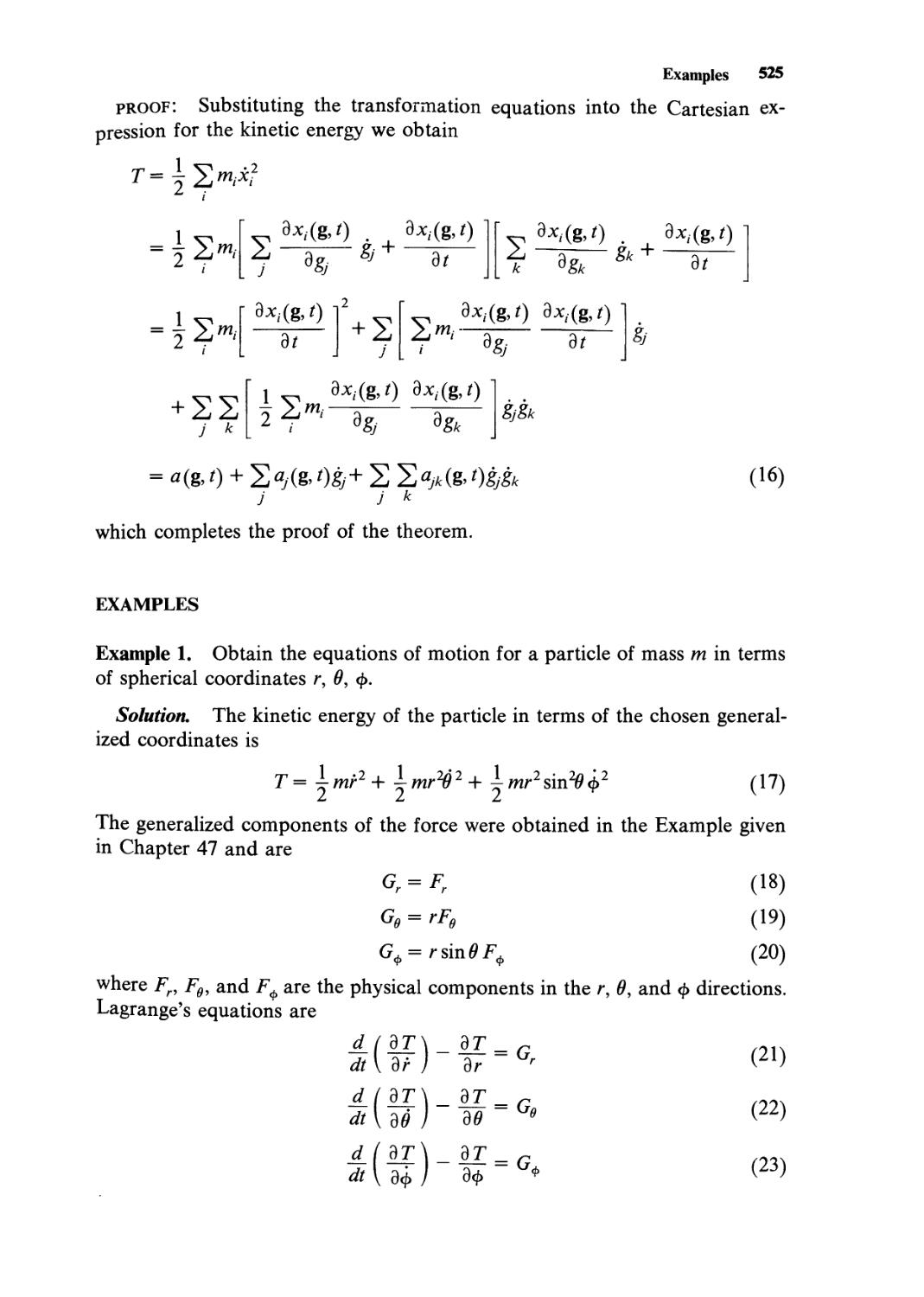
EXAMPLES
Example 1. Obtain the equations of motion for a particle of mass m in terms
of spherical coordinates r, 0, <J>.
Solution. The kinetic energy of the particle in terms of the chosen
generalized coordinates is
T= ±mr2+ -krnr202+ ±mr2 smftQ2
(17)
|mr2+ ^mr202 + }-™»2'
The generalized components of the force were obtained in the Example given
in Chapter 47 and are
Gr = Fr (18)
Ge = rFe (19)
G+ = rsin0F# (20)
where Fr, F9, and F^ are the physical components in the r, 9, and <j> directions.
Lagrange's equations are
d(dT\ 97\
A (dT\_uj_=r
dt\dr ) dr r
At ST]-!*!- r
dt\d9) 99 '
d_( <yr\ _ 9r = r
dt \ 8<j> ) 9<J> *
(21)
(22)
(23)
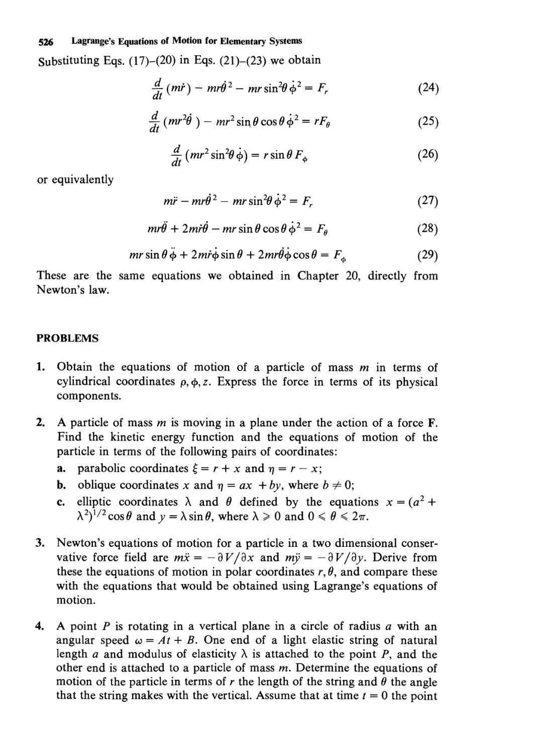
526 Lagrange's Equations of Motion for Elementary Systems
Substituting Eqs. (17)-(20) in Eqs. (21)-(23) we obtain
■j- (mr) - mr92 - mr sin20 <j>2 = Fr (24)
j-t (mr29 ) - mr2 sin 9 cos 0 <j>2 = rF9 (25)
jr (mr2 sin20 <j>) = r sin 9 F^ (26)
or equivalently
mr — mrO 2 — mr sin20 <j>2 = Fr (27)
rar# + 2mr0 — mr sin 9 cos 0 <j>2 = F9 (28)
mr sin 0 <£ + 2rar<j> sin 0 + 2mr0<j> cos 0 = F^ (29)
These are the same equations we obtained in Chapter 20, directly from
Newton's law.
PROBLEMS
1. Obtain the equations of motion of a particle of mass m in terms of
cylindrical coordinates p,<j>,z. Express the force in terms of its physical
components.
2. A particle of mass m is moving in a plane under the action of a force F.
Find the kinetic energy function and the equations of motion of the
particle in terms of the following pairs of coordinates:
a. parabolic coordinates £ = r + x and tj = r — x;
b. oblique coordinates x and tj = ax + by, where b ^ 0;
c. elliptic coordinates X and 9 defined by the equations x = (a2 +
A2)1/2cos0 and y = X sin 0, where X > 0 and 0 < 9 < 2m.
3. Newton's equations of motion for a particle in a two dimensional
conservative force field are mx = — dV/dx and my = — 3F/3j. Derive from
these the equations of motion in polar coordinates r, 9, and compare these
with the equations that would be obtained using Lagrange's equations of
motion.
4. A point P is rotating in a vertical plane in a circle of radius a with an
angular speed to = At + B. One end of a light elastic string of natural
length a and modulus of elasticity X is attached to the point P, and the
other end is attached to a particle of mass m. Determine the equations of
motion of the particle in terms of r the length of the string and 9 the angle
that the string makes with the vertical. Assume that at time / = 0 the point
Problems 527
P is at its lowest point, and that the motion of the point P and the mass m
lie in the same vertical plane.
5. Use Lagrange's equations to determine the equations of motion of a
particle with respect to a Cartesian frame S' that is rotating with a
constant angular velocity with respect to an inertial frame S. Assume that
the z axis is the axis of rotation and that the z and zr axes coincide.
49
Constraint Forces
INTRODUCTION
If a dynamical system is moving under the action of a force and the force is a
known function of the set of generalized coordinates g, the set of generalized
velocities g, and the time t, we can use Lagrange's equations for elementary
systems to determine g and g as functions of the time. In many situations,
however, a force is described not in terms of what it does to a system but in
terms of what it prevents the system from doing. For example, if a particle is
confined to remain on a particular surface, we are not ordinarily given the
value of the force the surface exerts on the particle; rather we are simply told
that the surface exerts whatever force is necessary to constrain the particle to
remain on it. In such cases the value of the force can usually be found only
after we have solved for the motion. In this chapter we develop techniques for
handling certain classes of such forces.
GIVEN FORCES AND CONSTRAINT FORCES
A given force or an active force is a force that is a known function of the
configuration and motion of the system on which it is acting and possibly also
the time.
A constraint force or a. passive force is the force exerted by an agent, called a
constraint, that responds to the action of a dynamical system in such a way as
to prevent it from assuming certain configurations or making certain
displacements.
In solving a particular problem the constraint forces cannot ordinarily be
handled in the same fashion as a given force, since we usually cannot
determine the exact value of the constraint force until after we have solved for
the motion of the system. It is therefore sometimes helpful to distinguish
between the given forces and the constraint forces in the equations of motion.
When we wish to make this distinction we retain the notation G to designate
the given forces, but use the notation R to designate the constraint forces.
528
Ideal Constraint Forces 529
GEOMETRIC AND KINEMATIC CONSTRAINT FORCES
A geometric constraint force is a constraint force that limits the possible
configurations of a system.
A kinematic constraint force is a constraint force that limits the possible
displacements of a system.
Every geometric constraint force will also be a kinematic constraint force,
since it is impossible to restrict the possible configurations of a system without
at the same time restricting the possible displacements of the system. However
it is possible to restrict the displacements without restricting the
configurations; therefore a kinematic constraint force is not necessarily a geometric
constraint force.
Let us consider some examples of geometric and kinematic constraint
forces. If a particle is enclosed in a box, the walls of the box act as a
constraint, and the force the walls exert in containing the particle is a
geometric constraint force. If a particle is constrained to remain on a
particular surface, the normal force the surface exerts on the particle is a geometric
constraint force. If a ball rolls on a two dimensional flat rough surface without
slipping, the normal force the surface exerts on the object is a geometric
constraint force because it limits the position of the center of mass to a
particular plane. But, in addition to this constraint, the tangential force due to
the roughness of the surface is a purely kinematic constraint force that couples
the rotational motion of the ball to the translational motion of the center of
mass. That is, because of the roughness of the surface, the center of mass of
the ball cannot undergo an infinitesimal translation in a particular direction
without an accompanying rotation of the ball. This constraint force is purely
kinematic because despite the roughness of the surface, it is always possible to
roll the ball on the surface in such a way that the final position of the center
of mass and the final orientation of the ball are completely arbitrary; therefore
the roughness of the surface does not impose a geometric constraint on the
ball. The tangential force exerted by a rough surface is not necessarily a
purely kinematic constraint. If for example a ball or cylinder rolls on a flat
rough surface without slipping, and in addition the motion is constrained to be
uniplanar, then in this case all the forces, including the tangential force
exerted by the surface, are geometrical constraints.
IDEAL CONSTRAINT FORCES
If the work done by a constraint force in any virtual displacement that does
not violate the constraint condition is zero, the constraint force is said to be an
ideal constraint force. Some important ideal constraint forces are listed below.
1. The internal forces that maintain the interparticle distances in a rigid
body fixed are ideal constraint forces. To show this consider a rigid
dynamical system consisting of N particles. Let r(oi) be the position of
530 Constraint Forces
particle i with respect to the origin of coordinates, r(y) the position of
particle j with respect to particle /, and t(ij) the force particle i exerts on
particle j. The virtual work done by the internal forces in a virtual
displacement of the system is
sw = 22»(i0 'WJ) (1)
' j
According to the law of action and reaction and Postulate V (Chapter 27)
m=-Hji) = c(uy(v) (2)
where c(ij) is a scalar. If we make use of Eq. (2), then Eq. (1) can be
rewritten
8^=SSc((0r(«y)-«r(i0 (3)
' j
The condition that the interparticle distances remain fixed can be stated
mathematically as follows:
r(y) • r(y) = constant (4)
If the virtual displacement 8r(ij) is to be consistent with the constraint
condition, Eq. (4), it must satisfy the condition
r(y) • 8r(ij) = 0 (5)
If we substitute Eq. (5) in Eq. (4) we obtain
8W=0 (6)
The constraint is thus an ideal constraint.
2. If a body is constrained to remain in contact with a smooth surface, the
force exerted by the surface on the object is an ideal constraint force. This
follows immediately from the fact that in a virtual displacement that is
consistent with the constraint, the point on the body that is in contact
with the surface can move only in a direction that is tangent to the surface
while the reaction force of the surface on the body is normal to the
surface. It should be noted that the constraint force is ideal even if the
surface is moving. The fact that the surface is moving does not alter the
argument above, since a virtual displacement is made at a fixed time.
Although the virtual work done on the constrained object by the moving
surface is zero, the actual work done is not generally zero.
3. If a body rolls without slipping on a surface, the force exerted by the
surface on the body is an ideal constraint force. This follows from the fact
that in a virtual displacement that is consistent with the constraint the
point on the body that is in contact with the surface is at rest, and
therefore the force exerted by the surface on the object does no work.
4. If two parts of the same object are smoothly hinged together, the resultant
of the pair of forces acting at the hinge is an ideal constraint force. This
follows from the fact that the respective forces exerted on the two parts by
Holonomic Constraint Forces 531
their mutual interaction are equal in magnitude, opposite in direction, and
are applied at a common point; therefore, in a virtual displacement that is
consistent with the constraint, the virtual work done by the constraint on
the one part is the negative of the virtual work done on the other part. The
net virtual work done on the system by the constraint force is therefore
zero.
HOLONOMIC CONSTRAINT FORCES
A holonomic constraint force is an ideal geometric constraint force that restricts
the possible configurations of a system to those that satisfy an equation of the
form
*(&') = ° (7)
or equivalently it is an ideal kinematic constraint force that restricts the
possible displacements of a system to those that satisfy an equation of the
form
?lAi(g,t)dgi+Ao(g,t)dt = 0 (8)
i
where the quantity S/^/(g>0^& + A0(g,t)dt is an exact differential or can be
made exact by multiplying it by some function of g and t.
To show the equivalence of the definitions above we note first that if Eq. (7)
is true, all displacements must satisfy the condition
<fo = 2, 8 d&+ dt dt = 0 (9)
Thus the conditions in the second definition are satisfied. Conversely if the
quantity 2/^/(g>0^/ + ^o(g>0^ is an exact differential (see Appendix 11),
there exists a function <j> such that
d<$> = *ZAi(g,t)dSl+A0(%,t)dt (10)
i
If in addition Eq. (8) is true the function <j> satisfies the equation
d<j> = 0 (11)
From Eq. (11) it immediately follows that there exists a <J> satisfying Eq. (7).
This completes the proof of the equivalence of the two definitions.
In the definition above we have assumed that the constraint force limits the
configurations to those that satisfy a single equation <j>(g, t) = 0. It is possible
of course that a constraint might limit the configurations to those that satisfy a
set of equations <$>x{g,t) = 0, <f>2(g,0 = 0, . . . . To handle this case we simply
break the force the constraint is exerting into component forces and associate
one force with each constraint equation. Thus if there are M constraint
conditions, there will be M constraint forces.
532 Constraint Forces
Examples of holonomic constraint forces are the internal forces that
maintain the interparticle distances in a rigid body fixed, and the force that
constrains an object to remain in contact with a smooth surface.
A nonholonomic constraint force is a constraint force that is not holonomic.
Some authors restrict the meaning of the term "nonholonomic" to a particular
class of constraint forces that are not holonomic; we refer to this class as
anholonomic.
ANHOLONOMIC CONSTRAINT FORCES
An anholonomic constraint force is an ideal kinematic constraint force that
restricts the possible displacements of a system to those that satisfy an
equation of the form
IlAi(g,t)dgi+A0(g,t)dt = 0 (12)
i
where the quantity 2/^/(8» 0¾ + ^o(g>0 is not an exact differential nor can
it be made exact by multiplying it by some function of g and t.
If an object is rolling on a perfectly rough surface and the motion is not
restricted to uniplanar motion, the force that prevents the object from slipping
is an anholonomic constraint force.
THE GENERALIZED COMPONENTS OF HOLONOMIC
AND ANHOLONOMIC CONSTRAINT FORCES
Although we cannot generally write down an expression for a particular
constraint force acting on a system as a function of g, g, and t before we have
solved for the motion of the system, we can sometimes take a step in that
direction. In particular, in the case of holonomic and anholonomic constraint
forces, we can determine the generalized components of a constraint force to
within a common scalar multiplicative function. The following theorem states
this fact precisely.
Theorem 1. If a dynamical system consisting of TV particles is subjected to a
holonomic or an anholonomic constraint force R, which restricts the possible
displacements of the system to those that satisfy the equation
3N
*ZAidgi+A0dt = 0 (13)
where the quantities A0,AU . . . , A3N are known functions of g and t, the
generalized components Rl9R2, . . . , R3N of the constraint force R satisfy the
equations
The Generalized Components of Holonomic and Anholonomic Constraint Forces 533
or equivalently there exists a quantity X, called a Lagrange multiplier, such
that
*/ = H (15)
for all values of i from 1 to 3N.
proof 1: Let Sg be a virtual displacement that is consistent with the
constraint. From Eq. (13) it follows that
24*&-0 (16)
i
And since the constraint force is ideal, the virtual work done by the constraint
force in a virtual displacement that is consistent with the constraint is zero,
that is,
2*/«&=0 (17)
i
Since the set of 3N 8gt must satisfy both Eqs. (16) and (17), only 3 N - 1 of the
8gi are independent. Let us choose the components Sg2, ..., 8g3N as the
independent components. To eliminate Sgx from Eqs. (16) and (17) we
multiply Eq. (16) by R} and Eq. (17) by Ax and take the difference of the
resulting equations. We obtain
'2[RlA1-R1Al]Sgl=0 (18)
/ = 2
Since the components 8g2, . . . , 8g3N are all independent, the coefficients of
each of the 8gi in Eq. (18) must be zero. It follows that
T, = a~ i = 2'--->3N (19)
The set of Eqs. (19) is equivalent to the set of Eqs. (14). Thus the first part of
the theorem has been proved. We next note that if Eq. (14) is true, there exists
a quantity X defined by the equation
X~T, (20)
that satisfies the second part of the theorem. This completes the proof.
proof 2: We could have alternatively but equivalently proved the theorem
as follows. If we multiply Eq. (16) by an arbitrary quantity X and subtract the
result from Eq. (17) we obtain
2W-H)«»=o (21)
/
Equation (21) must be true for arbitrary values of X and any 37V — 1 of the
variables gu g2, . . . , g3N. If we choose X such that
R.-XA^O (22)
534 Constraint Forces
then Eq. (21) becomes
2(^-^,)^/=° (23)
/ = 2
This can be true for arbitrary values of the 3 N - 1 variables Sg2, . . . , 8g3N
only if
R.-XA^O i = 2, . . . , 3N (24)
Combining Eqs. (22) and (24) it follows that there exists a X such that Eq. (15)
is satisfied. This completes the proof.
DEGREES OF FREEDOM
Our interest in the chapters that follow is primarily in systems that are acted
on by given forces, and holonomic or anholonomic constraint forces.
A dynamical system consisting of N particles that is subjected to L
anholonomic constraint forces and M holonomic constraint forces is said to
have 3N — L — M degrees of motional freedom and 3N — M degrees of
configurational freedom. Thus the number of degrees of motional freedom is equal to
the number of independent displacements Sg, that are required in addition to
the constraint conditions, to uniquely specify a particular displacement Sg.
And the number of degrees of configurational freedom is equal to the number
of independent generalized coordinates g,- that are required, in addition to the
constraint conditions, to uniquely specify the configuration g of the system.
Most authors do not distinguish between degrees of motional freedom and
degrees of configurational freedom, but simply use the phrase "degrees of
freedom" to mean one or the other of these types of degrees of freedom. In
reading other texts one should therefore be careful to find out what the author
means by "degrees of freedom." If the only constraint forces acting on a
system are holonomic constraint forces, as is most often the case, the number
of degrees of motional freedom and the number of degrees of configurational
freedom are equal, and in this case one can speak simply of degrees of freedom
without any danger of ambiguity.
EXAMPLES
Example 1. A disk of radius a rolls without slipping on a horizontal plane.
The plane of the disk remains vertical but is free to rotate about a vertical axis
through the center of the disk. Discuss the constraints.
Solution. In addition to the internal forces, which maintain the disk rigid
and are holonomic constraints, there is a constraint that holds the disk
vertical, a constraint that keeps the center of the disk a fixed distance above
the plane, and a set of constraints that keep the disk from slipping. To discuss
Examples 535
the latter constraints we choose an inertial frame S, with origin 0 in the
horizontal plane, 1 and 2 axes also in the horizontal plane, 3 axis vertically up,
and a frame S fixed in the disk, with origin O at the center of the disk, I and 2
axes in the plane of the disk, 3 axis perpendicular to the plane of the disk. We
then let e1? e2, e3, ey, e2, and e3 be the unit vectors in the 1,_2, 3, T, 2, and 3
directions, respectively; xl9 x2, and x3 be the coordinates of O with respect to
the frame S; 0 be the angle between e3 and e3; <J> the angle between the vector
e3 X e3 and the vector ej; and \j/ the angle between the vector ey and the vector
e3 X e3. The angles 0, <j>, and t// as chosen are the Euler angles, which were
used in the discussion of rigid body motion. The constraint that holds the disk
vertical can be represented by the equation
9 = f (25)
This is a holonomic constraint. The constraint that keeps the center of the disk
a fixed distance above the plane can be represented by the equation
x3 = a (26)
This is a holonomic constraint. The constraint that keeps the disk from
slipping can be obtained by noting that if the disk cannot slip, the velocity of
the point P on the disk that is in contact with the surface must be at rest with
respect to the point O. If we let \(OP) be the velocity of P with respect to O,
\(00) be the velocity of O with respect to O, and \(0P) be the velocity of P
with respect to 0, this condition becomes
\(0P) = \(00 ) + \(0P) = 0 (27)
But
\(00 ) = e^j + e2x2
and (see Chapter 6)
v(OP) = (e3t//) X (- e3a) = exa\p cos <$> + e2a\p sin <$>
Substituting Eqs. (28) and (29) in (27) we obtain
i:, + a\j/ cos <j> = 0
x2 + a\p sin <j> = 0
or equivalently
dxx + a cos<}> d\fj = 0
dx2 + a sin <f> d\p = 0
(28)
(29)
(30)
(31)
(32)
(33)
The differentials above are not exact differentials. Furthermore since it is
always possible to roll the disk on the surface in such a way that jc, , x2, <f>, and
*P take on any arbitrary value, the constraints represented by Eqs. (32) and
(33) are purely kinematic constraints; hence there are no functions that can by
multiplication convert the differential expressions in Eqs. (32) and (33) into
536 Constraint Forces
exact differentials. It follows that the constraints represented by Eqs. (32) and
(33) are anholonomic constraints. If we enumerate all the constraints acting
on the disk, we find that it is a system with four degrees of configurational
freedom and two degrees of motional freedom.
PROBLEMS
1. Two rigid bodies are moving in space. A rigid massless rod joins by means
of smooth ball-and-socket joints a given point of one body to a given
point of the other body, and one of the bodies is constrained to roll
without slipping on a given fixed surface. How many degrees of motional
freedom, and how many degrees of configurational freedom, does the
system have?
2. A disk is constrained to roll without slipping along a prescribed curve on a
horizontal surface. The plane of the disk is constrained to remain vertical
and tangent to the curve on the horizontal surface. How many degrees of
motional freedom does the system have? How many degrees of
configurational freedom does the system have? Express the rolling constraint in the
form of a differential equation, and determine whether the constraint is
holonomic or anholonomic.
3. A sphere of radius a is free to roll on a perfectly rough horizontal plane.
Discuss the constraints.
4. A sphere of radius a is constrained to roll without slipping on a vertical
plane that is free to rotate about a vertical axis in the plane. Discuss the
constraints.
5. A sharp-edged wheel of radius a is rolling on a rough horizontal surface.
Its instantaneous position is determined by assigning values to: (1) the
coordinates x, y of the point of contact of the wheel with the surface,
referred to a rectangular coordinate system x,y,z whose x-y plane
coincides with the surface, (2) the angle 0 between the axle of the wheel
and the z axis, (3) the angle § between the x axis and the intersection of
the plane of the wheel and the surface, and (4) the angle \p that the radius
toward the instantaneous point of contact of the wheel makes with an
arbitrary fixed radius. Show that the rolling constraint requires that
8x = acos<f> S\p and Sy = a sin <j>S\p. Show that these conditions cannot be
reduced to equations between the coordinates themselves, hence that the
constraint is anholonomic.
6. A particle of mass m is sliding on a smooth wire that is bent in the form of
a parabola, the equation of which is x2 = lay. If the value of x at
arbitrary time t is x(t), and the value of the x component of the constraint
force is Rx(t), what is the value of thej component of the constraint force
at time /?
Problems 537
7. A bead of mass m is moving on a smooth wire that is bent in the form of a
helix the equations of which in cylindrical coordinates p, <j>, z are z = a<j>
and p = b, where a and Z> are constants. How are the p, <j>, and 2
generalized components of the constraint force related?
8. A particle of mass m is constrained to move on the inner surface of a
smooth paraboloid of revolution, the equation of which is x1 + y1 = 2az.
How are the x, y, and z components of the constraint force related?
50
Lagrange's Equations of Motion
for Holonomic Systems
INTRODUCTION
Lagrange's equations of motion for an elementary system, which we derived in
Chapter 48, are not of much practical use when we are dealing with systems
containing a large number of particles, since the more particles we have, the
more equations we have to solve. However if the system is acted on by a large
number of holonomic constraints and has as a result only a few degrees of
freedom, as would be the case for example with a rigid body, then the problem
can be enormously simplified, as we see in this chapter.
HOLONOMIC SYSTEMS
A dynamical system that is acted on by forces that are either given forces or
holonomic constraint forces is called a holonomic system.
DEGREES OF FREEDOM
Let us consider a holonomic system in which there are N particles and M
holonomic constraint conditions. Let g = gl9 g2, . . . , g3N be a set of
generalized coordinates for the system of particles, and let
*i(&0 = 0, <f>2(&0 = 0, . . . , <f>M(g,t) = 0 (1)
be the M constraint conditions. Of the 37V coordinates g}, g2, . . . , g3N, only
3N — M are independent. The number 37V — M, which we designate by the
letter /, is defined as the number of degrees of freedom. Alternatively, we can
define the number of degrees of freedom as the minimum number of
coordinates required in addition to the constraint conditions to determine the
538
Generalized Components of a Force 539
configuration of the system. Note that in the case of holonomic systems there
is no difference between degrees of motional freedom and degrees of configu-
rational freedom, and therefore there is no ambiguity involved in using the
term "degrees of freedom."
GENERALIZED COORDINATES
Let us consider further the system discussed in the preceding section. Of the
37V coordinates g = gx, g2, . . . , g3N, only / = 3N - M are independent. Let
us designate a particular set of / of the coordinates as q = quq2, . . . , qf and
let us assume that the set q together with the constraint conditions uniquely
determine the configuration of the system. It then follows that the coordinates
gi can be written as functions of the set of coordinates q and the time t, that is,
&-&(*') (2)
The coordinates qt are completely independent. The coordinates gi are not.
The set of Eqs. (2) implicitly contains the constraint conditions and therefore
may be considered to define the constraint conditions.
Any/coordinates qx,q2, • • • , q/ that together with the constraint conditions
uniquely specify the configuration of a holonomic system of f degrees of
freedom, are called generalized coordinates for the holonomic system, and their
time rates of change quq2> • • • > ?/ are called generalized velocities for the
holonomic system.
CONFIGURATION SPACE
The motion of a dynamical system consisting of N particles can be
represented by the motion of a point in a 37V dimensional configuration space g.
The motion of a holonomic system having f degrees of freedom can be
represented by the motion of a point in an f dimensional subspace q of the
total configuration space. We refer to this subspace as a configuration space
for the holonomic system. The motion of the representative point in the space
g is governed by Lagrange's equations of motion for elementary systems. In
this chapter we derive the equations that govern the motion of the
representative point in the space q.
GENERALIZED COMPONENTS OF A FORCE
In Chapter 47 it was pointed out that the generalized component of a force
corresponding to a particular generalized coordinate gt depends not only on gi
but on the whole set of coordinates g = gx, g2, . . . , g3N in the same sense that
a partial derivative depends not only on the quantity varied but also on the
540 Lagrange's Equations of Motion for Holonomic Systems
quantities that are held constant. Since the set of generalized coordinates q
that are used to define the configuration of a holonomic system do not by
themselves constitute a complete set of generalized coordinates for the system
of particles, it follows that the generalized components of the force
corresponding to the coordinates q are not uniquely determined by our previous
definition, which is contained in Theorem 1 in Chapter 47. We can avoid this
difficulty by simply restricting the virtual displacements of a holonomic
system to those that do not violate the constraint conditions. Such virtual
displacements are uniquely determined by the set of displacements 8q= 8qu
8q2, . . . , 8qf. With this restriction we can then modify Theorem 1 in Chapter
47 as follows.
Theorem 1. Let us assume that we are given a holonomic system that has /
degrees of freedom and is acted on by a force. The virtual work 8W of the
force in an arbitrary virtual displacement Sq, which does not violate any of the
constraint conditions, can be written in the form
w-2a«fc (3)
i
where the quantities g,, g2, . . . , Qj depend only on the value of the force
and the constraint conditions. The quantities g,, g2, . . . , Qj are called the
generalized components of the force acting on the holonomic system. The set
of such quantities is designated Q, and the force whose generalized
components are the set Q is called the force Q acting on the holonomic system.
proof: The proof follows the same lines as the proof of Theorem 1 in
Chapter 47.
The following theorems give us some useful properties of the generalized
components g.
Theorem 2. If g,, g2, . . . , Qj and gr, Q2, . . . , Qj are two sets of
generalized components for a force Q acting on a holonomic system, corresponding
to the two sets of generalized coordinates qx,q2, . . . , qj and qv,q2>, . . . , q^,
and if the two sets of generalized coordinates are related by the
transformation equations
then the two sets of generalized components of the force are related by the
transformation equations
a.^¥«n^...».0 (5)
proof: The proof of this theorem follows the same lines as the proof of
Theorem 2 in Chapter 47.
Lagrange's Equations of Motion for Holonomic Systems 54*
Theorem 3. Consider a holonomic system containing N particles and having
f degrees of freedom. Let g = gl9 g2, . . . , g3N be a set of generalized
coordinates for the system of particles, and q = qx,q2, . . . , <7/ a set of generalized
coordinates for the constrained system, and let the transformation equations
between the set q and the set g be given by
& = &(*0
(«)
If Gl5G2, . . . , G3N are the generalized components of a force acting on the
system of particles, the generalized components g,, g2, . . . , Qj of the force
are given by
G-2<r
J
H
(7)
proof: The virtual work done in an arbitrary virtual displacement Sg is
given by
SW=^GjSgj (8)
j
If the values of the displacements Sg, are restricted to those that are consistent
with the constraints, then
(9)
Substituting Eq. (9) in Eq. (8) we obtain for the work done in a virtual
displacement that is consistent with the constraint
w=*z
H
(10)
Equation (7) follows immediately from Eq. (10).
Theorem 4. The generalized components g,, Q2, . . . , Qf of the constraint
forces acting on a holonomic system are zero.
proof: The constraint forces acting on a holonomic system are holonomic
constraint forces. By definition the work done by such forces in a virtual
displacement that is consistent with the constraint is zero.
LAGRANGE'S EQUATIONS OF MOTION FOR HOLONOMIC SYSTEMS
We are now in a position to determine the equations of motion for a
holonomic system. The result is stated in Theorem 5. The following lemma is
used in the proof of Theorem 5.
542 Lagrange's Equations of Motion for Holonomic Systems
Lemma 1. Let g = gx, g2, • • • , g$N be a set of generalized coordinates for a
dynamical system. If the system is a holonomic system and if q = qx,
q2, . . . , qj is a set of generalized coordinates for the holonomic system, then
dg/(q.<i>0
d_
dt
and
3&(q,4,/) 3&(q,0
H
H
(11)
(12)
proof: The proof is perfectly analogous to the proof of Lemma 1 in
Chapter 48.
Theorem 5. Consider a holonomic system having / degrees of freedom,
whose configuration is defined by the set of generalized coordinates q = qx,
q2, . . . , qj. If the system is acted on by a given force Q, the equations of
motion of the system are
A
dt
dT(q,q,t)
Hi
ZT(q,q,t)
H
= Qi
(13)
where 7"(q,q, t) is the kinetic energy of the constrained system. We refer to
these equations as Lagrange's equations for holonomic systems.
note: We give two proofs of the theorem. Each proof brings out different
aspects of the theorem.
proof 1: Consider a dynamical system consisting of N particles that is
acted upon by a given force G and a set of M holonomic constraint forces
R,,R2, . . . , RM. Let g = gl9 g2, . . . , g3N be an arbitrary set of generalized
coordinates that uniquely specifies the configuration of the system, and
fl — ?i>?2> • • • > ?/ a set °f / — 3N — M generalized coordinates that together
with the M constraint conditions uniquely specify the configuration of the
system. The equations of motion for the set g are
dt
3r(ftg,Q
3r(g,g,Q
9£
-^ +2**
(14)
where Rkj is the g. component of the constraint force R^. If we multiply Eq.
(14) by 9§-(q,0/3?/ anc* sum overy we obtain
3r(ft*.0
2
j
A
dt
94/
dgj{q,t) _ 3r(g,g,0 dgj(q,t)
H
Zgj
3ft
Vr9^0 dgj(q,t)
(15)
Lagrange's Equations of Motion for Holonomic Systems 543
The quantity 2;G,[3g,(q, 0/3ft] is just Qh the q,- generalized component of the
given force G, and the quantity Syi^g/q.O/Sft] is just the qt generalized
component of the constraint force Rk and is zero by virtue of Theorem 4.
Thus
Tr9^q10_
2GJ-!a--Q<
(16)
(17)
Now consider the left hand side of Eq. (15). If we rearrange the first term,
using the relation (dA/dt)B = d(AB)/dt — A(dB/dt), and then make use of
Lemma 1 we obtain
2
j
i dt
*T(g,g,t)
Hj
HjM ar(g,g,o dgj(q,t)
H
aS
4 dt
*T(g,g,t) 3§.(q,0
Hj
3ft
3g7(q>0
3ft
-2
3ft
3r(ftg,0 3§(q,0
9§
3ft
A.
dt
2
r 3r(g,g,Q 3g;(q,q,Q
a*
3v"(q,q,Q
3ft
3ft
3^,4,0
3ft
2
j
dT(g,g,t) dgj(q,t)
hj
3ft
(18)
If we substitute Eqs. (16)-(18) in Eq. (15) we obtain Eq. (13), which is the
desired result.
proof 2: Consider a dynamical system consisting of N particles that is
acted on by a given force G and a set of M holonomic constraint forces
Ri,R2, ..., RM. Let g = gu g2, . . ., g3N be an arbitrary set of generalized
coordinates that uniquely specify the configuration of the system. The
equations of motion of the system are
d_
dt
37-(8,8-0
3 7X& g, 0
= 6/ + 2¾
3& *
Now let us assume that the constraint equations are given by
**(&') = ° k= 1,2,..., M
(19)
(20)
544 Lagrange's Equations of Motion for Holonomic Systems
The constraint force R^ restricts the displacements to those that satisfy the
equations <j>k(g,t) = 0. If we take the differential of this equation we see that
the constraint force R^ restricts the displacements to those satisfying the
equations
2j —^— d&+ —= = °
(21)
It follows from Theorem 1 in Chapter 49 that the gt component of the
constraint force R^ is given by
Rkt - K'
3&
Substituting Eq. (22) into Eq. (19) we obtain
3r(ftg.O
A
dt
Hi
(22)
(23)
Now suppose we choose as our generalized coordinates the set
g = £l> #2> • • • >g3N = ?1>?2> • • • ><l3N-M><i>l><i>2> ■ ■ ■ > *A/ = 4 * (24)
where the set q is any set of 3N — M generalized coordinates that together
with the M constraint conditions uniquely determine the configuration of the
system. The corresponding set of generalized components of the given force G
will be designated:
G = G1?G2, . . . , G3N = g„ Q2, • • • , Qsn-m, *i,*2> > ®m = Q,* (25)
With this choice for the generalized coordinates the equations of motion
become
A.
dt
d
dt
■ dT(q,q,<j>,<j>,t) -
' dT(q,q,<j>,j>,t) '
3*,
_ ar(q,q,<j>,<jM)
dT{q,q,<$>,$,t)
Hi
-Q,
= ¢.- + \
(26)
(27)
Equations (26) and (27) provide us with 3N equations in the 3N + M
unknowns q{,q2, • • • , ?3/v-m> <h>4>2> • • • > 4>m> ^i>^2> • — >^m- Tne constraint
equations
¢, = 0 (28)
provide the necessary additional equations. If we substitute Eqs. (28) in Eqs.
(26) we obtain
d_
dt
9 T(q, q,0,0,Q
H
9r(q,q,0,0,Q
= fi,-
(29)
But T(q, q, 0,0, /) = T(q, q, /) is the kinetic energy the system would have if it
were constrained to the surfaces <J>j = 0, <j>2 = 0, . . . , <j>M = 0. Furthermore the
Lagrange's Equations for Elementary Systems and Holonomic Systems 545
Q. are defined by the requirement that the virtual work be given by
sw-2G-*ft+2***** (30)
/' k
It follows that 2/2/½ is tne work done in a virtual displacement in which
<j>v<j>2, . . ., and <f>M are held constant. But holding 4>,,4>2, • • • , and <j>M
constant is equivalent to considering only virtual displacements that are
consistent with the constraints. This completes the proof.
THE RELATIONSHIP BETWEEN LAGRANGE'S EQUATIONS FOR
ELEMENTARY SYSTEMS AND LAGRANGE'S EQUATIONS FOR
HOLONOMIC SYSTEMS
The motion of a dynamical system consisting of TV particles can be
represented by the motion of a point in a 37V dimensional configuration space g. The
motion of the representative point in the space g is governed by Lagrange's
equations for elementary systems, which we discussed in Chapter 48. If the
system is a holonomic system having / degrees of freedom, where/< 37V, the
motion of the system can be represented by the motion of a point in the /
dimensional subspace q. The motion of the representative point in the sub-
space q is governed by Lagrange's equations for holonomic systems. Formally
these equations appear to be identical with Lagrange's equations for
elementary systems. There are however important differences. In the first place the
expression for the kinetic energy appearing in Lagrange's equations for
elementary systems assumes the possibility of completely arbitrary motions of
the particles in the system, whereas the expression for the kinetic energy
appearing in Lagrange's equations for holonomic systems is the kinetic energy
associated with the constrained motion of the system. In the second place the
generalized component of the force appearing on the right hand side of
Lagrange's equations for elementary systems includes contributions from the
constraint forces as well as the given forces and is defined in terms of the work
done in an arbitrary virtual displacement, while the generalized component of
the force appearing on the right hand side of Lagrange's equations for
holonomic systems includes contributions from the given forces only and is
defined in terms of the work done in a virtual displacement that is consistent
with the constraints.
Although Lagrange's equations for holonomic systems are applicable only
when the constraint forces are holonomic, they represent a tremendous
simplification over Lagrange's equations for elementary systems in the cases
of systems that consist of large numbers of particles that are subjected to large
numbers of holonomic constraints. Consider for example a rigid body
consisting of TV particles. The number 37V - M in this case is six, and thus only six
equations are required to determine the motion.
One might ask which set of equations is more fundamental. On the one
hand, one could argue that Lagrange's equations for elementary systems are
546 Lagrange's Equations of Motion for Holonomic Systems
more fundamental because there are no restrictions on the nature of the
forces, and therefore the equations apply to a wider class of problems. On the
other hand one can apparently derive Lagrange's equations for elementary
systems from Lagrange's equations for holonomic systems by simply
reclassifying all the holonomic constraint forces as given forces. In this case there
would be 37V degrees of freedom, and the equations of motion obtained would
be identical to the generalized equations of motion.
The source of the paradox rests in our failure to note that when constraint
forces are involved, Lagrange's equations of motion for elementary systems
represent an incomplete set of equations, because the generalized components
of the constraint forces are not completely known before solving for the
motion and therefore we have too few equations for the number of unknowns.
Thus when we speak of Lagrange's equations for elementary systems as being
more fundamental we are implicitly including with these equations whatever
constraint conditions are necessary to provide us with as many equations as
we have unknowns. On the other hand if we start with Lagrange's equations
for holonomic systems, we cannot reclassify a holonomic constraint force as a
given force unless we also introduce the appropriate constraint equations.
EXAMPLES
Example 1. A bead moves on a smooth wire that is bent in the form of a
vertical circle of radius a. The wire rotates about a fixed vertical diameter with
a uniform angular velocity co. Find the equation of motion of the bead.
Solution. Let r, 0,<j> be the spherical coordinates of the bead, and let the
origin be at the center of the circle and the polar axis vertically down. The
kinetic energy in terms of these coordinates is
T={mr2 + {mr202 + {mrhm20^2 (31)
The bead is not free but is subject to the constraints
r = a (32)
<j> = co (33)
The two constraints are holonomic, hence the system is a holonomic system
with one degree of freedom. We choose 0 as our generalized coordinate.
Substituting Eqs. (32) and (33) in Eq. (31) we obtain
T(0j ) = \ma202 + ±rnaWsin20 (34)
The work done in a virtual displacement that is consistent with the constraints
is
8W= mgd(acosO)= -rngasm686 (35)
Hence
Q9 = — mga sin 6 (36)
Problems 547
Lagrange's equation is
A.
dt
dT(0,9)
3770,0)
-^r2 = a (37)
Substituting Eqs. (34) and (36) in Eq. (37) we obtain
ma20 — ma2co2sin 0 cos 0 = — mga sin 0 (38)
or equivalently
0 - co2sin 0 cos 0 + -£ sin 0 = 0 (39)
The motion of the bead can be determined by solving this equation for 0 as a
function of time.
PROBLEMS
1. Two rods AB and BC of lengths a and b, respectively, are freely jointed
at B and hang in a vertical plane from A, which is fixed. Choosing the
angles 0 and <j> that the respective rods make with the vertical, determine
the generalized components of a horizontal force of magnitude F acting
at C.
2. Discuss the motion of a simple pendulum, taking in turn the following
generalized coordinates: the angular displacement, the horizontal
displacement, and the vertical displacement.
3. A bead of mass m is free to slide on a smooth helical wire the equation of
which in cylindrical coordinates is p = a, z = b<$>. Gravity is acting in the
positive z direction. The particle is released from rest at the point p = a,
<t> = 0, z = 0. Determine z as a function of the time.
4. A bead of mass m slides along a smooth wire bent into the form of the
parabola y = x2. Gravity is acting in the negative y direction. The plane
of the wire rotates about the y axis with a constant angular speed w. At
time t = 0 the bead is at the point x = a,y = a2, and is not moving in the
y direction. Obtain equations with which one could determine x as a
function of the time.
5. A particle of mass m is supported by a frictionless horizontal disk that
rotates about a vertical axis through its center with a constant angular
velocity <o. The particle is connected by a massless string of length a to a
point located a distance b from the center of the disk. Show that the
motion of the particle with respect to the disk is similar to that of a
simple pendulum, and find the frequency of small oscillations of the
system.
6. Two particles of masses m and M, respectively, are connected by a
massless rod of length a. The particle of mass m is constrained to move
548 Lagrange's Equations of Motion for Holonomic Systems
on the surface of a sphere of radius b, and the particle of mass M is
constrained to move along the vertical diameter of the sphere. Choose an
appropriate set of generalized coordinates and obtain the equations of
motion.
7. A particle is constrained to move on a smooth surface in the form of the
anchor ring x = p cos \p, y = p sin \f/, z = b sin 0, where p = a + b cos 0 and
a > b. Prove that if there are no forces except the reaction of the surface,
motion around the outer equatorial circle will be stable, and that if this
motion is slightly disturbed the new path will cross the equator at
intervals of length ir\b{a + Z>)]1/2. Show also that motion around the
inner equatorial circle is unstable, and that if such motion is slightly
disturbed the path of the particle will cross the outer equatorial circle at
an angle 2arctan(Z?/a)1/2.
8. A uniform rod of mass m and length 2a is held with one end on a
smooth floor and the other end against a smooth wall. Rectangular
Cartesian axes are chosen so that the wall is the plane x = 0, the floor is
the plane z = 0, and the ends of the rod are at the points (2a, — /J, 0) and
(0, /J, 2y), respectively. Prove that if the rod is released from rest in this
position, the initial downward acceleration of the center of mass is
(3g/4)[(a2 + 4yS2)/(«2 + 4,62 + Y2)]-
9. One end of a uniform rod AB of mass m and length 2a is constrained to
move on a smooth straight horizontal wire, and the rod is constrained to
move in the vertical plane containing the wire. The rod is acted on by
gravity and a force of magnitude F acting at B in a direction parallel to
the wire. Let x be the distance of A from a fixed point on the wire, and 9
the angle the rod makes with the downward vertical. Determine the
equations of motion of the rod in terms of the variables x and 0.
10. A uniform rod OA of mass m and length 2a is pivoted at O. A bead P of
mass am slides on the rod and is joined to O by a light elastic string of
unstretched length a and spring constant nmg/a. Let x be the distance
OP, 0 the angle the rod makes with the downward vertical OZ, and <J> the
angle which the plane AOZ makes with a fixed vertical plane. Write
down Lagrange's equation of motion for the system in terms of the
variables x, 9, and <J>. Show that if a steady motion is possible with
0 = 7r/3, and x = 4a/3, then <j>2 = 3g/2a and n = 6a.
11. The ends A and B of a uniform rod of mass m and length 2a are
constrained to remain on a smooth circular wire of radius b, where
b > a. The wire is made to rotate with a constant angular speed Q, about
a fixed vertical axis passing through the center C of the wire. Using as a
generalized coordinate 0, the angle the rod makes with the horizontal,
obtain Lagrange's equation of motion.
51
The Determination of Holonomic
Constraint Forces
INTRODUCTION
If we are given a holonomic system, we can use Lagrange's equations for
holonomic systems to determine the motion of the system. The big advantage
gained by using these equations rather than Lagrange's equations for
elementary systems is the elimination of the constraint forces from consideration.
Sometimes however we are interested in the value of a particular constraint
force.
In this chapter we show how one can in this case obtain the desired
constraint force.
THE DETERMINATION OF A HOLONOMIC CONSTRAINT FORCE
If we are given a system in which there are TV particles and M holonomic
constraint conditions, and we wish to determine the constraint force
associated with the Mth constraint condition but are not interested in the
constraint forces associated with the first M-l constraints, we simply treat the
first Af-1 constraint forces as we would any set of holonomic constraint
forces, but we treat the Mth constraint force as if it were a given force. If we
do this and also make use of the relation developed in Chapter 49 between a
constraint condition and the corresponding components of the constraint
force, we will be able to solve not only for the motion of the system but also
for the Mth constraint force. This technique is summarized in the following
theorem.
Theorem 1. Consider a system consisting of N particles, acted on by a given
force, and M holonomic constraint forces. If q = ql9q2, • • • , ^3n-m+i *s a set
of generalized coordinates that together with the first M — 1 holonomic
constraint conditions uniquely determine the configuration of the system, then
549
550 The Determination of Holonomic Constraint Forces
the A/th constraint condition can be written in the form
4>(q,t) = 0
and the generalized coordinates qt satisfy the set of equations
A.
dt
9r(q.q>0
H
= a+A
d<Kq,Q
(1)
(2)
where A is a function of the time, T(q, q, t) the kinetic energy, and Qi the qt
generalized component of the given force. Equations (1) and (2) provide us
with 3N - M + 2 equations in the 3N - M + 2 unknowns quq2, . . . ,
<73A/-a/+i anc* K and can thus be used to find the q({t) and \{t). The
generalized components Rt of the constraint force associated with the
constraint condition (1) are given by
3<f>(q, t)
proof: If we treat the A/th constraint force, which we designate R, as a
given force, and make use of Lagrange's equations of motion for a holonomic
system, we obtain
A.
dt
9r(q,q,Q
dT(q,q,t)
= 0, +#,
(4)
where jRf. is the qt component of R. But from the results of Chapter 49 the qf
component of R is given by Eq. (3). This completes the proof of the theorem.
EXAMPLES
Example 1. A bead of mass m is free to slide on a smooth helical wire, the
equations of which in cylindrical coordinates are p = a, z— b<j>. Gravity is
acting in the positive z direction. The particle is released from rest at the point
p = a, <j> = 0, z = 0. Determine as a function of § the z and § physical
components of the reaction force the wire exerts on the bead.
Solution. The kinetic energy of the bead in terms of the coordinates p, <f>,
and z is
T=imp2 + \mp24>2 + ±
2Lrap" + \mp"<$>" + \mz" (5)
The bead is subject to the holonomic constraints
p - a = 0 (6)
z - b<f> = 0 (7)
The system is a holonomic system with one degree of freedom. If we choose z
as the generalized coordinate, the kinetic energy function is
T(z,z) = \m
a2+b2
(8)
Examples 551
and the bead is acted on by a given force whose z generalized component is
Qz = mg
Lagrange's equation for the system is
A.
dt
dT(z,z)
dz
dT(z,z)
dz
-a
Substituting Eqs. (8) and (9) in Eq. (10) we obtain
a2 + b2 ,
m-
■ z = mg
Solving Eq. (11) and applying the boundary conditions we obtain
,_ gbV
2( a2 + b2)
Combining Eqs. (7) and (12) we obtain
,_ gbt2
2(a2 + b2)
(9)
(10)
(11)
(12)
(13)
This approach tells us nothing about the constraint force. Suppose that instead
of proceeding as above we treat the force associated with the constraint
z = b<f> as a given force; then the system is subject only to the constraint p = a
and is thus a holonomic system with two degrees of freedom. Choosing z and
<j> as generalized coordinates, the kinetic energy function is obtained by setting
p = a in Eq. (5). Thus
T(z,<j>J,<j>) = \mal$L + \mz
(14)
The bead is now acted on by the gravitational force, the z and <j> components
of which are
Q2 = mg
0., = 0
(15)
(16)
and by the force due to the constraint z — Z><j> = 0, the components of which
are related as follows:
RZ = X
(17)
(18)
where X is an unknown parameter. Lagrange's equations in this case are
A.
dt
A.
dt
3T(z,<^,i
dz
dT(z,<t>,z
,<*>)
,<i>)
d<j>
dT(z
dT(z
,<f>,z
dz
,<M
,4»)
,<?>)
a<>
-& + R*
(19)
(20)
552 The Determination of Holonomic Constraint Forces
Substituting Eqs. (14)-(18) into Eqs. (19) and (20) we obtain
mi = mg + \ (21)
ma2$=-\b (22)
These two equations together with the constraint equation
z = b4> (23)
provide us with three equations in the three unknowns z, <f>, and A. If we solve
for z and <J> we obtain the same results given by Eqs. (12) and (13). If we solve
for X we obtain
X=-^-2 (24)
a2+b2 V }
Substituting Eq. (24) in Eqs. (17) and (18) and noting that the physical
components Fz and F^ of the reaction force are related to the generalized
components Rz and R^ by the relations Rz = Fz and R^ = pF^ we obtain
PROBLEMS
1. The radius r of a soap bubble is changing with time according to the
equation r = at + b, where a and b are constants. A particle of mass m is
constrained to remain on the surface. At t = 0 the particle is given a
tangential velocity v. Find the path of the particle and the reaction of the
surface.
2. A particle is constrained to move in a smooth plane that is rotating with a
constant angular velocity to about a horizontal axis in the plane. Find the
distance r of the particle from the axis of rotation as a function of the
time, and also the reaction of the plane on the particle as a function of
time.
3. A particle of mass m is constrained to move along a rough wire bent into
the form of a horizontal circle of radius a. The coefficient of kinetic
friction is ju, and the particle is initially moving with a speed v0. Find the
angular position of the particle as a function of the time, and the reaction
of the wire on the particle. Assume gravity is not acting.
4. A particle of mass m is constrained to move along a smooth wire bent into
the form of a horizontal circle of radius a and is subject to an air
resistance of magnitude mkv2, where k is a constant and v is the speed of
Problems 553
the particle. The particle is initially moving with a speed v0. Find the
angular position of the particle as a function of the time, and the resultant
reaction of the wire on the particle. Assume gravity is not acting.
5. A smooth wire is bent into the form of a helix the equations of which, in
cylindrical coordinates, are z = a<}> and p = b, where a and b are
constants. The origin is the center of an attractive force that varies directly as
the distance. Determine the equation of motion of a bead that is free to
slide on the wire, and find the p, <f>, and z physical components of the
reaction force of the wire.
6. A particle slides down a smooth stationary sphere, under the action of
gravity, from a position of rest at the top. Use Lagrange's equations to
find the reaction of the sphere at any value of 0, where 6 is the angle
between the vertical diameter of the sphere and the normal to the sphere
that passes through the particle. Find the value of 6 at which the particle
falls off.
7. A uniform solid cylindrical drum of mass M and radius a is free to rotate
about its axis, which is horizontal. An inextensible cable of negligible mass
and length I is wound on the drum, and carries on its free end a mass m.
Write down the Lagrangian function in terms of an appropriate
generalized coordinate, assuming no slipping of the cable. The cable is initially
fully wound up, and the system is released from rest with the mass in the
same horizontal plane as the axis of the cylinder. Find the angular velocity
of the drum when it is fully unwound. By treating the length I of the cable
as a variable, and finding Lagrange's equations for two generalized
coordinates, show that the tension in the cable is Mmg/(M + 2m).
8. A particle of mass m is at rest on top of a smooth paraboloid, the equation
of which is x2 + y1 — a(a — z), where a is a constant and the z axis is
vertically up. The particle is displaced slightly from its equilibrium
position and slides down the surface. Choosing cylindrical coordinates p, <j>,
and z as generalized coordinates, write down Lagrange's equations of
motion. Determine the constraint force. At what height will the particle
leave the paraboloid?
9. A solid cylinder A of radius a and mass m is at rest on top of a fixed
cylinder B of radius b. The axes of the two cylinders are parallel and
horizontal. The cylinder A is displaced from its equilibrium position and
rolls without slipping down cylinder B. Use Lagrange's equations of
motion to determine the constraint forces, and find the position at which
the cylinders separate.
52
Lagrange's Equations of Motion for
Anholonomic Systems
INTRODUCTION
If the forces acting on a dynamical system are given forces or are holonomic
constraint forces, we can use Lagrange's equations for elementary systems or
Lagrange's equations for holonomic systems to determine the motion. If
however some of the forces are anholonomic constraint forces, we cannot
directly apply the equations above. The purpose of this chapter is to determine
how to handle these situations.
ANHOLONOMIC SYSTEMS
A dynamical system that is acted on by one or more anholonomic constraint
forces together with any other given forces or holonomic constraint forces is
called an anholonomic system.
LAGRANGE'S EQUATIONS OF MOTION FOR ANHOLONOMIC SYSTEMS
The equations of motion for anholonomic systems can be obtained by a
straightforward extension of the results we have already obtained.
Theorem 1. Consider an anholonomic system consisting of N particles, acted
on by a given force, M holonomic constraint forces, and L anholonomic
constraint forces. Let q= <7i,<72> • • • > #3n-m ^>e a set °f generalized
coordinates that together with the M holonomic constraint conditions uniquely
determine the configuration of the system. If the anholonomic constraint
forces Rl5R2, . . . , RL restrict the displacements to those satisfying the equa-
554
Determination of Anholonomic Constraint Forces 555
tions
*ZAki(q,t)dqi+AkO(q,t)dt = 0 (1)
i
or equivalently to those satisfying the equations
^Aki(q,t)q^Ako(q,t) = 0 (2)
i
where k ranges from 1 to L, then the motion of the system can be determined
by the 3N - M equations
A.
dt
dT(q,q,t)
3ft
37Yq,q,0 „
H =& + pA (3)
together with the L constraint equations (2), where T{q,q,t) is the kinetic
energy and Qt the qt generalized component of the given force. We refer to the
set of Eqs. (3) together with the set of Eqs. (2) as Lagrange's equations for
anholonomic systems.
proof: If we treat the anholonomic constraint forces as if they were given
forces and make use of Lagrange's equations for holonomic systems, we
obtain
dt
37^)1 *T(q,q,t)_
-^^\^H~-Qi + Vki (4)
where Rki is the q( component of the constraint force R^. But from the results
of Chapter 49, the q{ component of the constraint force R^ can be written
Rki = M*/ (5)
Combining Eqs. (4) and (5) we obtain the set of Eqs. (3). The set of Eqs. (3) is
a set of 37V — M equations in the 3N — M + L unknowns qi,q2, • • • > ?3;v-a/>
A1? A2, . . . , \L. The constraint equations (2) provide us with the necessary L
additional equations. This completes the proof of the theorem.
DETERMINATION OF ANHOLONOMIC CONSTRAINT FORCES
If we are given an anholonomic system consisting of N particles acted on by a
given force, M holonomic constraint forces, and L anholonomic constraint
forces R,,R2, . . . , RL for which the constraint conditions are 2/^w^?/ +
Akodt, the equations of motion consist of 3N - M + L equations in the
3N - M + L unknowns quq2, • • • , ?3;v-m>^i>^2> ---,^- These equations
can be used to solve not only for the qt as functions of time but also for the \k
as functions of the time. Knowing the Xk we can immediately write down the
?/ component of the constraint force R^ from the relation
Rki = \Aki (6)
556 Lagrange's Equations of Motion for Anholonomic Systems
Thus Lagrange's equations for anholonomic systems can be used not only to
determine the motion but also to determine the anholonomic constraint
forces.
EXAMPLES
Example 1. A disk of radius a and mass m whose plane is constrained to
remain vertical rolls on a perfectly rough horizontal surface, under the action
of a force f whose line of action passes through the center of the disk. Obtain
equations of motion for the disk.
Solution. This is the same system that was discussed in the Example given
in Chapter 49, where it was shown that the system has four degrees of
configurational freedom. A suitable set of generalized coordinates is the set xl9
x2, <t>, and \f/ defined in the above-mentioned example. In terms of these
coordinates the kinetic energy of the system is
T = i m (x] + jc|) + I ma\$2 + 2^2) (7)
There are two anholonomic constraints acting on the system that restrict the
displacements to those satisfying the equations
xx + ai//cos<j> = 0
x2 + a\p sin <j> = 0
or equivalently satisfying the equations
dxx + acos<j>d\p = 0
dx2 + a sin<J> dxp = 0
The generalized components of the force f are
&,=/.
QXi = fi
0«=0* = o
Applying Lagrange's equations for anholonomic systems we obtain
mxx =/i+Ai
m*2 =/2 + ^2
\mar§ = 0
\ma2^ = acos<j>\} + asm<f>\2
(8)
(9)
(10)
(11)
(12)
(13)
(14)
(15)
(16)
(17)
(18)
Equations (15)-(18) together with Eqs. (8) and (9) provide us with six
equations in the six unknowns xl9 x2, <J>, \p, A,, and X2.
Problems 557
PROBLEMS
1. The position of a particle of mass m is described by Cartesian coordinates
x,y,z. The particle is acted on by a force F and is subjected to an
anholonomic constraint that constrains the velocity in such a way that
y/x = z. Determine the equations of motion.
2. The position of a particle of mass m is described by Cartesian coordinates
x,y,z. The particle is acted on by a force F and is subjected to an
anholonomic constraint that constrains the velocity in such a way that
x—ty — a, where a is a constant. Determine the equations of motion.
3. A uniform disk of radius a and mass m rolls down a flat inclined surface
that makes an angle a with the horizontal. The disk is constrained so that
its plane is always perpendicular to the inclined plane, but it may rotate
about an axis perpendicular to the surface. Determine the motion of the
center of mass of the disk.
4. A disk of mass m and radius a is constrained to roll without slipping on a
horizontal plane. The disk is not constrained to remain vertical. Obtain
equations of motion.
5. Two thin homogeneous disks Dx and D2, each of mass m and radius a are
connected by a massless axle of length 2b. The disks are free to rotate
about the axle but are constrained to remain perpendicular to the axle.
The system rolls without slipping on a horizontal plane. Let x and y be the
coordinates of the midpoint of the axle with respect to a Cartesian
coordinate system with x and y axes fixed in the plane. Let 0 be the angle
on the x-y plane that the direction of the axle makes with the x axis, <j> be
the angle that a line passing from the center of Dx to a point fixed on its
circumference makes with the upward vertical, and \p be the angle that a
line from the center of D2 to a point fixed on its circumference makes with
the upward vertical. Show that the system has four degrees of configura-
tional freedom and two degrees of motional freedom. Obtain the
equations of motion in terms of the set of generalized coordinates x, y, 0, <j>.
6. A homogeneous sphere of mass M and radius a rolls without slipping on a
perfectly rough horizontal plane under the action of a force F whose line
of action passes through the center of mass. Determine the equations of
motion of the sphere.
53
Generalized Force Functions
note: Unless otherwise stated, in this and the following chapters we
restrict our attention to holonomic systems. Instead of constantly stressing the
fact that the systems are holonomic, we shall for the sake of simplicity of
terminology suppress reference to the holonomic nature of the system as much
as possible. Thus we shall simply speak of a system having / degrees of
freedom, whose configuration is defined by the set of generalized coordinates
Q — ?i > ?2> • • • > ?/ and whose motion can be determined by solving Lagrange's
equations.
INTRODUCTION
In many cases the generalized components for a particular force can be
derived from a single scalar function. The use of such functions can often
simplify the equations of motion and their solutions. In this chapter we
consider some general types of functions from which the generalized
components of a force can be derived.
GENERALIZED POTENTIALS
Theorem 1. Consider a dynamical system having / degrees of freedom. Let
Q— Q\> Qi> - - - > Qf anc* Q' = Qyy Qi'> • • > Qf be two arbitrary sets of
generalized components for a given force, corresponding to the two sets of
generalized coordinates q = q\,q2> • • • > <7/ and q' = qv,q2', • • • , <7/- K there
exists a quantity £/(q, q, t) such that
O = —
^ dt
9E/(q,q,Q
9C(q,q,Q
3ft
(1)
558
Generalized Potentials 559
Then the generalized components Qr will be given by
^ dt
3t/(q',qV)
9qr
(2)
The quantity U is called a generalized potential, and the given force is said to
be derivable from a generalized potential.
proof: From Theorem 2 in Chapter 50 we have
If we substitute Eq. (1) in Eq. (3) we obtain
(3)
fl-2 i
dt
-25
3£/(q,q,0
3f/(q,q,0 ] 39y(q',0
3¾
dqf
Hj
dqt
3¾
3*
If we rearrange the first term on the right hand side of Eq. (4) using the
relation (dA/dt)B = d(AB)/dt — A(dB/di), and make use of Lemma 1 in
Chapter 48, we obtain
&=2
1 dt
W(q,q,t) dqjtf.t)
H
v WM.Q d
^ *" dt
H
H-
9qf
-2
j
dU(q,q,t) 3$(q\/)
3<7y
3*
_ a y»
dU(q,q,t) dqj(q',q',t)
3¾
3<7,<
-2
j
dU(q,q,t) dqj(q',q',t) + dU(q,q,t) dqj(q',t)
dt
3¾
3f(q',q',Q
dq,
dqr dqj
W(q',q',t)
dqr
H'
(5)
This proves the theorem.
note: If F(q,q, t) is the total time derivative of any function F(q, t) then
^[3^(q,q,0/3*]/.<# - 9F(q,q, 0/9¾ = 0. (See Chapter 54.) Hence if *7 were
replaced by U + F, Theorem 1 would remain true.
560 Generalized Force Functions
The following corollary is an immediate consequence of Theorem 1.
Corollary 1. Consider a dynamical system having/ degrees of freedom. Let
Q = Q\, Qi, • • • , Qf and Q = Qy, Q2,, . . . , Qf be two arbitrary sets of
generalized components for a given force, corresponding to the two sets of
generalized coordinates q = qx,q2, . . . , qr and q' = qy,qr, •••>?/• If there
exists a quantity V(q, t) such that
the generalized components Qr will be given by
9V(qf,t)
Qi = -^r (7)
The quantity V is called a potential, and the given force is said to be derivable
from a potential.
The potential V(q, t) is simply a special case of the generalized potential
U(q, q, i). We have singled it out in a corollary because it represents the most
frequently encountered situation.
DISSIPATION FUNCTIONS
Theorem 2. Consider a dynamical system having f degrees of freedom. Let
Q = 2i> £?2> • • • > £?/ and Q' = Qv QT, . . . , Qf be two arbitrary sets of
generalized components for a given force, corresponding to the two sets of
generalized coordinates q = quq2, • • • , qj and q' = qvqT, . . . , qj>. If there
exists a quantity W(q, q, t) such that
a w2 (8>
the generalized components Q,, will be given by
dW(q',q',t)
«■ TCjr2 (9)
The quantity W is called a dissipation function.
proof: From Theorem 2 in Chapter 50
^-2¾^ (10)
Examples 561
If we substitute Eq. (8) in Eq. (10) and make use of Lemma 1 in Chapter 48
we obtain
= -2
7 H- a*
3^(q,q,Q 3$(q',q',0
7 H a?/'
3*F(q',q',0
(11)
3?/'
This proves the theorem.
EXAMPLES
Example 1. A particle of charge q is moving in an electromagnetic field
defined by the vector fields E and B, or equivalently by the scalar potential $
and the vector potential A, where E = — V$ — dA/dt and B = V x A. Show
that the generalized components of the electromagnetic force acting on the
particle can be derived from the generalized potential U = q$ — q\ • A.
Solution. To prove that U is a suitable generalized potential, we must show
that it leads to the correct expressions for the generalized components of the
force for some set of generalized coordinates. In terms of the Cartesian
coordinates xl9x2,x3 we have
U(x,x,t) = q<P(x,t) - q'ZxtAfat) (12)
Substituting this expression into the equation
a = —
*■> dt
dU(x,x,t)
dx
dU(x,x,t)
dx:
(13)
we obtain
-.2^-,^-,¾^¾ (.4)
On the other hand if we calculate the xl9 x2, and x3 components of the force
using the Lorentz expression
F = qE + qy x B = q{ - V<1> - M J + qy x (V X A) (15)
562 Generalized Force Functions
we obtain
where eiJk is the Levi-Civita symbol discussed in Appendix 6. Comparing Eqs.
(14) and (16) we obtain
Qj = Fi (17)
Thus for Cartesian coordinates the potential U = q$> — q\ • A leads to the
correct generalized components. From the results of this chapter it follows that
it will lead to the correct generalized components for any set of generalized
coordinates.
PROBLEMS
1. Obtain the equation of motion for a particle falling vertically under the
influence of gravity when frictional forces obtainable from a dissipation
function kv2/2 are present. Integrate the equation to obtain the velocity
as a function of the time and show that the maximum possible velocity for
fall from rest is v = mg/k.
2. A pendulum of length b with a bob of mass m is suspended from a spring
of unstretched length a and spring constant k. The point of support of the
pendulum is restricted to vertical motion. The bob is immersed in a
viscous medium that exerts a force whose direction is opposite to the
direction of motion of the bob and whose magnitude is proportional to the
speed of the bob. The proportionality constant is a. Obtain the equations
of motion of the particle in terms of y, the distance of the point of support
of the pendulum below its position when the system is in static
equilibrium, and 0, the angle the pendulum makes with the vertical.
3. A particle of mass m is moving under the action of a force that is
derivable from a potential V. Let xu x2, and x3 be the coordinates of the
particle with respect to an inertial frame S. Let x,y,z be the coordinates
of the particle with respect to a frame S' whose origin O and z axis
coincide with the origin O and 3 axis, respectively, of the frame S but
Problems 563
which is rotating about the z axis with constant angular speed co. Show
that the equations of motion of the particle in the frame S' can be
regarded as the equations of motion of a particle in a fixed coordinate
system acted upon by the force associated with the potential V and by a
force derivable from a generalized potential U. Hence find a velocity
dependent potential for the centrifugal and Coriolis forces.
54
Lagrange's Equations of Motion
for Lagrangian Systems
LAGRANGIAN SYSTEMS
In most of the dynamical problems encountered in physics, the constraint
forces are holonomic and the given forces are derivable from a generalized
potential. We refer to systems in which the constraint forces are holonomic
and the given forces are derivable from a generalized potential as Lagrangian
systems. Our interest in this chapter is in Lagrangian systems.
LAGRANGE'S EQUATIONS OF MOTION FOR LAGRANGIAN SYSTEMS
Theorem 1. Consider a Lagrangian system of / degrees of freedom. If we
define a quantity L, called the Lagrangian for the system, as follows:
L=T-U (1)
where T is the kinetic energy and U the generalized potential for the system,
then the motion of the system, in terms of an arbitrary set of / generalized
coordinates q = quq2, • • • , ft, can be determined by the equations
A
dt
3L(q,q,f)
3ft
^M=0 (2)
3ft
These equations are called Lagrange's equations of motion for Lagrangian
systems, or frequently simply Lagrange's equations.
564
The Lagrangian 565
proof: Since a Lagrangian system is a holonomic system, the motion is
governed by Lagrange's equations for holonomic systems,
A
dt
^-»
From the definition of the generalized potential U,
O = —
^ dt
3£/(q,q,Q
9q,
at/(q,q,/)
-isr- (4)
If we combine Eqs. (1), (3), and (4) we obtain Eq. (2), which completes the
proof.
THE LAGRANGIAN
If a particular dynamical system is acted on by a set of holonomic constraint
forces and a given force that is derivable from a generalized potential, and if
we know the configuration and motion of the system at some instant of time,
we can in principle determine the configuration and motion at some later time
by solving Lagrange's equations. In setting up Lagrange's equations for a
particular problem there are two major steps. The first step is to choose a set
of independent generalized coordinates q, that together with the constraint
conditions uniquely determine the configuration of the system. Such a set is
said to define the configuration of the system. The second step is to determine
the Lagrangian L as a function of q, q, and t. Once we know L(q,q, t) we can
write down the equations of motion. Thus we say that the Lagrangian
function L(q,q, t) defines the behavior of the system under the action of the
given force. It is important to note that L must be known as a function of q, q,
and t if we wish to determine the behavior of the system. Knowing the
Lagrangian as a function of some other set of variables is not necessarily
equivalent to knowing the Lagrangian as a function of q, q and t. It is for this
reason we say that the Lagrangian function L(q,q, t) defines the behavior of
the system, rather than saying that the Lagrangian L defines the behavior of
the system.
Instead of defining the Lagrangian L as the difference between the kinetic
energy T and the generalized potential U, it is possible to generalize the
definition by simply defining the Lagrangian as any quantity that when
expressed as a function of q, q, and t and substituted into Lagrange's equation
that is, Eq. (2)—leads to the correct equations of motion. In this spirit it is
566 Lagrange's Equations of Motion for Lagrangian Systems
interesting and sometimes useful to note that one can add the total time
derivative of any function F(q, t) to the Lagrangian without altering the
equations of motion. To prove this we note first that
and thus
. <*F(*0 „ 8f(q,() . ^ 3F(q,l)
dt *i da, V ' 3?
3^(¾ q,Q _ 32F(q,Q . 3^(q,Q
3¾ f 3^,3¾ *' 3¾3?
3F(q,q,/) 3F(q,/)
A
dt
3¾
3F(q,q,f)
3^~
3ft
3^0 32F(q,0
= 2J a„ a„ ft+
y 3¾-3ft
dt
3F(q,q,f)
3ft
3^(q,q,Q
3ft
dtdq;
= 0
(5)
(6)
(7)
(8)
(9)
EXAMPLES
Example. A hoop of mass M, moment of inertia Mk2 about an axis through
its center, and radius a, rolls without slipping on a horizontal plane. A particle
of mass m is suspended from the center of the hoop by a string of length b.
The motion of uniplanar. Find the equations of motion.
Solution. The system has two degrees of freedom. We choose as
generalized coordinates the angle 9 that a particular radius of the hoop makes with
the vertical, and the angle <j> that the string makes with the vertical. The kinetic
and potential energy functions are
T(9,4>J,j>) = \[M(a2 + k2) + ma2]92 + \mb2$2 - mab94>cos<}> (10)
V(9,4>)= -mgb cos 4> (11)
The Lagrangian function is
L(9,4>,9,i>) = \[M(a2 + k2) + ma2]92 + \mb2§2 - mab9j>cos<f>
+ mgb cos <j>
(12)
Lagrange's equations are
ns are
A.
dt
A
dt
30
' 3L(0,<M,<i>) "
dL(O,<j>,0,i>)
do
dL(0,<f>,0,i>)
Problems 5ff7
(13)
(14)
Substituting Eq. (12) in Eqs. (13) and (14) we obtain
[M(tf2+ k2) + ma2]0 -mab$cos¢ + mabj>2sm<j> = 0 (15)
mb2<$> — mab9 cos § + mgb sin <J> = 0 (16)
We thus have two equations in the two unknowns 0 and <j>, which can be
solved to give us 0{t) and <j>(t).
PROBLEMS
1. A particle of mass m is suspended by a massless rod of length b from a
support P, which moves uniformly on a vertical circle of radius a with
constant angular speed co. Assuming that the motion of the system is
restricted to the vertical plane containing the circle, determine the
equation of motion of the system.
2. A bead of mass m moves on a smooth wire bent into the form of a
horizontal circle. The radius of the circle varies with time according to
the equation r = at2 + b. One point P on the circle remains fixed, and
the direction of the diameter through P remains fixed. Determine the
equation of motion of the bead.
3. A cone of mass M and vertical angle 2a can move freely about its axis,
which is vertical. The cone has a fine smooth groove cut along its surface
so as to make a constant angle /? with the generating lines of the cone. A
particle of mass m is free to slide in the groove. The system is initially at
rest, with the particle a distance c from the vertex. Show that if 0 is
the angle through which the cone has turned when the particle is a
distance r from the vertex, then {Mk2 + mr2sin2a)/(Mk2 + mc2sm2a) =
exp(20sinacot /?), where Mk2 is the moment of inertia of the cone
about its axis.
4. A thin wire of mass M is bent in the form of the helix x = a cos \p,
y = a sin ty, z = a\p tan /?, and is mounted so as to be free to rotate about
the z axis, which is horizontal. The length of the wire is such that the
center of mass lies on the axis. A small smooth ring of mass m slides on
568 Lagrange's Equations of Motion for Lagrangian Systems
the wire. The wire is at rest when the ring is projected horizontally along
the wire from the lowest position on it with velocity aco. Show that if co is
not too large the plane through the axis and the ring oscillates like a
simple pendulum of length a(M + rasin2/?)/(Mcos2/? + msm2/3) and
that the wire turns through an angle (mo)T sm2/3 cos /?/(Mcos2/? +
msin2/3) in each period T of the pendulum motion.
5. A particle of mass m is attached to a fixed point on a rough horizontal
table by a massless spring of unstretched length a and spring constant k.
The particle is constrained to move on a straight line passing through the
fixed point. The coefficient of friction for the contact between the
particle and the surface is jit. Find a Lagrangian that will give the correct
equation of motion when used in Lagrange's equation.
6. A particle of mass m can slide freely on a light wire bent into the shape
of the curve a3y = x4 which can rotate about the y axis, which is
vertically upward. If a steady motion takes place with the particle at
x = a, find the angular velocity Q, of the wire. If the wire is constrained
to rotate with the steady angular velocity £2, and the particle is slightly
disturbed from its steady motion at x = a, show that it will oscillate
about this position with a period of oscillation 27r(\la/Sg)^2. Find the
period of oscillation if the wire is not constrained but moves freely about
the y axis.
7. A system is composed of three particles of equal mass m. Between any
two of them there are forces derivable from a potential V = — a exp( —
br\ where r is the distance between the two particles and a and b are
constants. In addition, each of two of the particles exerts a force on the
third that can be obtained from a generalized potential of the form
U = — c\ • r, where v is the relative velocity of the interacting particles
and c is a constant. Set up the Lagrangian for the system using as
coordinates the radius vector R of the center of mass, and the two
vectors px = rx — r2, and p2 = r2 — r3. Is the total angular momentum of
the system conserved?
8. Show that the equations of motion of a charged particle in an
electromagnetic field are unaffected by a gauge transformation.
9. A uniform rod OA of mass m and length la is pivoted at O. The rod
makes the angle 0 with the downward vertical OZ and the plane AOZ
makes the angle <J> with a fixed vertical plane. A bead P of mass am
slides on the rod and is joined to O by a light elastic string of natural
length a and modulus of elasticity nmg. Choosing x = OP, 6, and <j> as
generalized coordinates, obtain Lagrange's equations of motion and
show that if steady motion is possible with 6 = it/3 and x = 4a/3, then
<f>2 = 3g/2a and n = 6a.
Problems 569
10. Two uniform rods AB and BC, each of mass m and length 2a, are
smoothly joined at B. The rod AB is free to rotate about A, which is
fixed; C can slide freely along a horizontal line through A, and the plane
of the rods is vertical and is free to rotate about a vertical axis through A.
Let 9 be the angle the rod AB makes with the horizontal (where 9 is
positive when the rod is below the horizontal), and \f/ the angle the plane
of the rods makes with a fixed vertical plane through A. Obtain the
equations of motion of the system in terms of the coordinates 9 and \p. If
at time t = 0, 9 = it/4, 9 = 0, and \p = Q, show that at any later time
4a92(\ + 3sin20) = 4att2(2 - sec20) - 3g[V2 - 2sin0] and that B
initially rises if 22 > 3(2)]/2g/\6a.
11. A solid homogeneous cylinder of mass m and radius a rolls without
slipping down the inclined plane face of a wedge of mass M, which in
turn rests on a perfectly smooth horizontal floor. The angle between the
inclined surface and the horizontal is a, and the entire motion takes
place in a plane perpendicular to the floor and containing the normal to
the inclined plane. Use Lagrange's equations of motion to find the
acceleration of the wedge.
12. A circular cylinder of radius a and mass m rolls without slipping inside a
horizontal semicircular groove of radius b cut in a block of mass M. The
block is constrained to move without friction in a vertical guide, and is
supported by a spring of spring constant k. Taking as coordinates the
vertical displacement x of the block and the angular displacement 9 of
the center of the cylinder, both measured from the position of static
equilibrium, determine by means of Lagrange's equations the equations
of motion of the system.
55
Lagrange's Equations of Motion and
Tensor Analysis
INTRODUCTION
In this chapter we show how the techniques of tensor analysis can be used to
obtain the equations of motion of a particle in terms of an arbitrary set of
coordinates, and the relationship between these equations and Lagrange's
equations. The reader who is not familiar with general tensors should read
Appendix 23 at this point because the concepts and notation of Appendix 23
are used throughout this chapter. Although for simplicity our analysis is
restricted to a single particle, the results can be readily extended to a system of
particles.
NEWTON'S LAW IN TENSOR FORM
If we can express a physical law in terms of a particular set of coordinates,
and if we know the law of transformation between this set of coordinates and
a second set of coordinates, we can use this transformation to express the
given law in terms of the second set of coordinates.
If we can express a physical law by an equation, each of whose sides is a
tensor of the same kind, the form of the equation will be invariant when we
transform from one coordinate system to another; hence it becomes a simple
job to change coordinates. It is therefore highly desirable though not necessary
to be able to express a physical law in tensor form.
How does one go about expressing a law in tensor form? One way is to find
an equation written in tensor form that for a particular set of coordinates
reduces to a form that is known to be correct in that coordinate system. This is
the technique we use to write Newton's law in tensor form.
570
Lagrange's Equations of Motion 571
Newton's law in Cartesian coordinates for a single particle can be written
The quantity xl is not a general tensor. However, the quantity dxi/dt is a
contravariant vector, since
dxl _ s? dxl dxi n.
dt f 3jc; dt W
or equivalently (using the notation of Appendix 23)
UX n V UXJ ,1 s.
dT-9JdT (3)
which is the law of transformation for a contravariant vector. Although
dxl I dt is a tensor, d2xl /dt2 is not a tensor, since the ordinary derivative of a
tensor with respect to a scalar is not necessarily a tensor. If, however, we take
the absolute derivative of dxl/dt with respect to t we will obtain a tensor.
Hence
8 ( dxl\
8t\ dt )
u X ■ -p/ uXJ uX /a\
~^ + lJkdTir w
is a contravariant vector. Furthermore for Cartesian coordinates the Tl-k vanish
and 8(dxi/dt)/8t reduces to d2xl/dt2. It follows that we can write Eq. (1)
dt2 J dt dt J v J
If we now define the vector /' as the contravariant vector whose components
in Cartesian coordinates are the usual components of the force, the right hand
side of Eq. (5) is also a contravariant vector.
Each side of Eq. (5) is now a tensor of the same kind. Furthermore Eq. (5)
gives the correct law of motion for Cartesian coordinates. It follows that Eq.
(5) is the correct law of motion for arbitrary coordinates xl. If we multiply Eq.
(5) by gin sum over /, and relabel indices, we obtain
™<r d2xj , wV dxj dxk f ,rx
m^^+mT^drir=fi (6)
which is the covariant form of Eq. (5).
LAGRANGE'S EQUATIONS OF MOTION
If we define
T = \mgJk ^- ^- ^\mgjkxJxk (7)
572 Lagrange's Equations of Motion and Tensor Analysis
and note that
^=^¼^ (8)
ox
1¾="%/*/ (9)
OX
= mgijXj + { m [ djgkl + dkgij]xJxk (10)
we obtain
i( g ) " J~ = mgyxJ + tm[djgu + dkgiJ - digjk]x^
= mgijV + {mTjKixJxk (11)
Substituting Eq. (11) in Eq. (6) we obtain
d_
dt
im-*L=fi (12)
\dxl) dxl J V }
Equation (12) is an alternate form of the equation of motion for arbitrary
coordinates. The equation of motion in this form is simply Lagrange's
equation of motion.
THE GENERALIZED COMPONENTS OF A FORCE
The covariant vector / is the covariant vector whose components in Cartesian
coordinates are the ordinary components of the force. From the analysis in the
preceding section it follows that the ft are equivalent to what we have been
referring to as the generalized components of the force. It follows that the
generalized components of a force are simply the components of the covariant
vector whose components in Cartesian coordinates are the ordinary
components of the force.
SECTION
Auxiliary Principles
of Lagrangian Mechanics
J
56
Constants of the Motion in the
Lagrangian Formulation
INTRODUCTION
In Chapter 33 we saw that solving the equations of motion for a dynamical
system is equivalent to finding the independent constants of motion.
Lagrange's equations can frequently be a great help in finding constants of motion
for they allow us to determine the equations of motion in terms of different
sets of coordinates, and the use of one set of coordinates can frequently reveal
a constant of motion that would be quite hidden if viewed from some other set
of coordinates.
In this chapter we consider the problem of finding constants of the motion
from the Lagrangian point of view. We restrict our attention to systems whose
behavior is defined by a Lagrangian.
CONSTANTS OF THE MOTION
Consider a dynamical system having f degrees of freedom. Let q = q\,q2,
• • . ,gy be a set of generalized coordinates for the system, and q= q\,q2>
• • . , qj the corresponding set of generalized velocities. Any function ^(q, q, t)
whose value remains constant during the motion of the system is called a
constant of the motion.
Theorem 1. There are exactly 2/ independent constants of motion for a
dynamical system having / degrees of freedom.
proof: The proof of this theorem follows the same lines as the proof of
Theorem 1 in Chapter 17.
575
576 Constants of the Motion in the Lagrangian Formulation
Theorem 2. If the behavior of a dynamical system having f degrees of
freedom is defined by a Lagrangian function L(q, q), which is not an explicit
function of the time, there are 2/ - 1 independent constants of the motion that
are not explicit functions of the time t.
proof: The proof of this theorem follows the same lines as the proof of
Theorem 2 in Chapter 17.
ENERGY
Theorem 3. Consider a dynamical system having f degrees of freedom whose
configuration is defined by the set of generalized coordinates q = qu
q2, . . . , qj. If the behavior of the system is defined by a Lagrangian function
^(q>q), which is not an explicit function of the time, the quantity
is a constant of the motion. If furthermore the generalized potential U is a
function only of q, and either the equations of transformation between the set
of Cartesian coordinates x and the set of generalized coordinates q are not
functions of the time or the kinetic energy T is a function of the set of
generalized coordinates q, and a homogeneous quadratic function of the set of
generalized velocities q, then
H(q,q)=T(q,q)+U(q) (2)
and therefore in this case T + U is a constant of the motion.
proof: The time rate of change of the quantity H is given by
dH _ v d
dt 41 dt
a£(q,q)
Hi
^, 9£(q>q).. ^, 3i(q,q) .
= 2I|
3^(q,q)
d^(q,q)
H
(3)
But from Lagrange's equations the term in the braces is zero and therefore
f =0 (4)
It follows that H is a constant of the motion. We have therefore proved the
first part of the theorem. To prove the second part we note first, from the
Generalized Momentum 577
definition of the Lagrangian, that
L=T-U (5)
and if U = C/(q), then
BL^q). ^ ar(q,q) .
We next note that if x = x(q) then T is a homogeneous quadratic function of
the generalized velocities qx,q2, • • • , ?/ (see Theorem 2 in Chapter 48). But if
T is a homogeneous quadratic function of the velocities qx,q2, . • • , <7/, then
from Euler's theorem, which is proved in Appendix 20, or by substituting
T= i2/SA?/?7 into the expression 2/[9T(q>q)/9?i]?/> we obtain
v9^q).
S-a^-*=2r (7)
Combining Eqs. (1), (5), (6), and (7) we obtain Eq. (2). This completes the
proof of the theorem.
GENERALIZED MOMENTUM
Consider a system of / degrees of freedom, whose behavior is defined by the
Lagrangian function L(q, q, t). The generalized momentum conjugate to the
generalized coordinate q( is defined as
Pl = ~W~ (8)
Note that if there are no constraints, and we choose the set of Cartesian
coordinates x as our generalized coordinates, and the generalized potential is
not a function of the velocity, the generalized momentum conjugate to the
coordinate x( ispi = m^. In this case the generalized momentum conjugate to
the coordinate xi is the same as the x( component of the ordinary linear
momentum. However it should be noted carefully that the generalized
momentum conjugate to a Cartesian coordinate xi is not in general equal to the x(
component of the linear momentum. Consider for example a particle of mass
w that is constrained to remain on the surface xx + x2 + x3 = 0 but is
otherwise free. If we choose xx and x2 as our generalized coordinates then
^== T= \mx\ + \mx\ + {m( — xx - x2)2 and thus px = 2mxx + mx2. As a
second example consider an unconstrained particle of mass m that is moving
in the potential U = Cxxxx, where C is a constant. The Lagrangian in this case
ls L = ±mx\ + \mx\ + \mx\ — Cxxxx and thus/?! = mxx — Cxx.
If the Lagrangian function is not an explicit function of a particular
generalized coordinate q{ the coordinate is said to be cyclic or ignorable.
578 Constants of the Motion in the Lagrangian Formulation
Theorem 4. The generalized momentum conjugate to a cyclic coordinate is a
constant of the motion.
proof: Starting with Lagrange's equations
A
dt
3L(q,q,0
we note that if L(q, q, t) is not a function of a particular coordinate qh then
3L(q,q,0
Combining Eqs. (8)-(10) we obtain
= 0 (10)
= 0 (11)
And thus the generalized momentum/?, conjugate to the cyclic variable qt is a
constant of the motion.
SYMMETRY AND CONSTANTS OF THE MOTION
If the Lagrangian function L(q,q,/) is not a function of a particular
coordinate, the behavior of the system does not depend on the value of that
coordinate, and the conjugate momentum is a constant of the motion.
Frequently we can determine a constant of motion for a system subject to a given
force without explicitly writing down the Lagrangian by noting from
symmetry arguments that the behavior of the system is unaffected by the change of a
particular coordinate. We shall consider two important cases.
In the following theorems we use the notation 3//3z, where z = e,Zj +
e2z2 + e3z3 is an arbitrary vector, to represent the quantity e! 3//3^1 +
e23//3z2 + e33//3z3.
Theorem 5. Consider a dynamical system consisting of TV particles. Let m(i)
be the mass of particle i. Let r(/) and v(/) be the position and velocity,
respectively, of particle i with respect to the origin of coordinates. If the
behavior of the system is defined by a Lagrangian function L(r, v, t) =
L[r(l), ..., r(N),v(l), ... , \(N),t] and if the Lagrangian function is
invariant under an arbitrary translation in a particular direction in space, the
component of the quantity 2/d£(r,v,/)/3v(/) in the direction of the
translation is a constant of the motion. If furthermore the generalized potential is not
a function of the velocities v(0, then ]T/3£(r,v,0/3v(0 = S/w0'M0 = P>
where P is the total linear momentum of the system with respect to the origin
of coordinates.
Symmetry and Constants of the Motion 579
proof: Consider a virtual displacement in which the system undergoes an
infinitesimal uniform translation c. Then
6r(l) = Sr(2)= • • • =8r(N) = e (12)
Sv(l) = 8v(2)= • • • =8v(N) = 0 (13)
If the Lagrangian is invariant under such a displacement then
„ dL(r,v,t) ^ 3L(r,v,/)
3.-(/)
BL^VM)
= e-2,^^ o
3v(i)
3r(/)
But from Lagrange's equations
dt
3L(r,v,/)
3v(0
and therefore
3L(r1v10=^
3r(/) i/
3L(r,v,f)
3£(r,v,Q
3v(/)
= 0
Substituting Eq. (16) in Eq. (14) we obtain
A.
dt
« -^2
This result must be true for arbitrary values of the magnitude of c. It follows
that
£ A. V
or
3L(r,v,f)
3v(0
values
3£(r,v,Q
3v(/)
3L(r,v,0
= 0
(14)
(15)
(16)
(17)
-y
e f 3v(/)
= 0
= 0
(18)
(19)
And thus the component of '£lidL(r,\,t)/d\(i) along the direction c/e is a
constant of the motion. If furthermore the generalized potential U is not a
function of the velocities v(z'), then
3L(r,y,f) 3r(r,v,Q
t 3v(/) f 3v(/)
= 2^(^2-(^(7)-(7)}
= 2W(0V(0 = P (20)
This completes the proof of the theorem.
580 Constants of the Motion in the Lagrangian Formulation
Theorem 6. Consider a dynamical system consisting of N particles. Let m(i)
be the mass of particle /. Let r(/) and v(/) be the position and velocity,
respectively, of particle i with respect to the origin of coordinates. If the
behavior of the system is defined by a Lagrangian function L(r,v, t)~
L[r(l), ..., r(N),v(l), ..., \(N\t] and if the Lagrangian is invariant under
an arbitrary rotation in space about a particular axis passing through the
origin of coordinates, the component of the quantity 2/r(0 X [3L(r,v,/)/
3v(/)] in the direction of the axis of rotation is a constant of the motion. If
furthermore the generalized potential is not a function of the velocities v(z')
then 2>(0 X [3L(r,v,0/3v(0] = 2>(0 X m(i)\(i) = H, where H is the total
angular momentum of the system with respect to the origin of coordinates.
proof: Consider a virtual displacement in which the system undergoes an
infinitesimal rotation c about a particular axis through the origin of
coordinates, where c is a vector whose direction is along the axis of rotation and
whose magnitude is equal to the angle of rotation. Then
(21)
(22)
8r(i) = c x r(/)
«*(/) = ex v(/)=4[ ex r(/)]
dt
If the Lagrangian is invariant under such a rotation, then
dL(r,\,t) „ dL(r,\,t)
= 2
8r(0
3L(r,v,/)
av(o
, „ dL(r,v,t) j _
■[«x-(0]+ 2-^4^0]
[exr(0]+2
[exr(0]
3v(/) dt
3L(r,v,0 d
3v(0
dt
[exr(/)]
= 0 (23)
This result must be true for arbitrary values of the magnitude of c, hence
3L(r,v,f)
A
dt
€ y v ' 3v(/)
= 0
(24)
Noether's Theorem 581
It follows that the component of 2/r(0 X [3L(r, v, t)/d\(i)] along the direction
€/e is a constant of the motion. The rest of the proof is the same as in the
proof of Theorem 5.
NOETHER'S THEOREM
All the results obtained in the preceding sections could have been obtained by
making use of the following theorem.
Noether's Theorem. Consider a system whose dynamical state at a given
instant of time t can be described by a set of generalized coordinates
q= <7p<72> • • • > ?/ and a set °f generalized velocities q = q\,q2> • • • > ?/ and
for which there exists a Lagrangian function L(t, q,q) that when substituted
into Lagrange's equations of motion determines the dynamical behavior of the
system. If it is possible to find a set of functions
T=T(t,q,q,e) (25)
Q = Q(*,q,q,£) (26)
where e is a time independent parameter, and
(^),.0= ' (27)
(Q)«-o-<i (28)
and if when the arguments /, q, and q in the Lagrangian function L(t, q, q) are
replaced, respectively, by r(/,q,q,e), Q(/,q,q,€) and Q(/,q,q,<M) where
■ __ dQ dQ/dt Q _Q(/,q,q,q,€)
V dT dT/dt f T(/,q,q,q,€) l ]
the resulting function satisfies the relation
£W^4q>*)>Q(^*q^ (30)
where F is the total time derivative of some function F(/,q,q), then the
quantity
^ 3L(/,q,q)
^ + S \? to-ifi-F (31)
where
€ =
9e
(32)
Je = 0
582 Constants of the Motion in the Lagrangian Formulation
and
9<2,-(',q.q><0
■ni =
3e
(33)
is a constant of the motion.
proof: Carrying out the derivative in Eq. (30) we obtain
^ 3L(r,Q,Q) 3&(*,q,q,€)
+ 2
3ft 3e
3(r,Q,Q) 3<2,(^,q,q,q,€)
3& d€
3L(r,Q,Q) 3T(;,q,q,£)
dT
3e
^ . 3f(/,q,q,q,€)
+ L(T,Q,Q)—K—e '-
= F
(34)
e = 0
To evaluate the terms in Eq. (34), we first expand T and Qt in powers of €,
obtaining
^=(^ = 0 +
a-(&)«_(>+
3r(f,q,q,€)
3ft(',q,q,0
e +
£ = 0
€ +
(35)
(36)
e = 0
Substituting Eqs. (27), (28), (32), and (33) in Eqs. (35) and (36) we obtain
T=t+ &+■■• (37)
ft = q, + 1,,6+--- (38)
From Eqs. (37) and (38) we obtain
7=1+^+--- (39)
ft = q, + 7j,€ + • • • (40)
From Eqs. (37)-(40) it follows that
(7-),=0=1 (41)
(2,),=0=¾ (42)
(&)--(tL-*
(43)
dT(t,q,q,e)
3e
r 3ft(',q,q,
df(t,
3ft('
3ftC
3e
qq.q>
3«
q,qq>
3e
-q.i<i
«)
0
*)
if)
= «
= u
le=0
= 1
Je = 0
= *?/
Noether's Theorem 583
(44)
(45)
(46)
(47)
: = 0
3e
_3_
3«
ft(f,q,q,q,e)
f(t,q,q,q,e)
e = 0
J_ 3g;(^q>q>q>e) _ ft 3r(/,q,q,q,e)
r
3€
f2
3«
J£ = 0
= U-4,I (48)
Using Eqs. (27), (28), (41)-(48) in Eq. (34) and noting also that
3L(r,Q,Q)
3ft
3L(T,Q,Q)
dT
3L(/,q,q)
H
3L(*,q,q)
37
[L(r,Q,0)]€_o = L(/,q,q)
(49)
(50)
(51)
we obtain
y ^LJt,q,q) L^3L(?,q,q) 3L(f,q,q)
(52)
In the remainder of the proof we suppress the argument of functions
appearing in a partial derivative, since in all cases the argument would be (/, q, q) and
there is very little chance of confusion. We now note
dL
H
L.> dldL-A d ( dL\-c dL~t
(53)
(54)
(55)
584 Constants of the Motion in the Lagrangian Formulation
Substituting Eqs. (53)-(55) in Eq. (52) we obtain
?st*+?
-2
+
AhV dt(dqir\
A*ttq*r Am)9*'nq*
dt
f v dL ■ 3L -
i H 3¾
which can be simplified to
9L
H
. _d_(dL\
'/ ^ { dqt )
?H
From Lagrange's equations
H dt { dqt )
Using Eq. (58) in Eq. (57) we obtain
^ + 2^0?,-^)-^
d_
dt
^ + 2ffu-^)-^
= 0
(56)
= 0 (57)
(58)
(59)
It follows that the quantity in square brackets in Eq. (59) is a constant of the
motion, which is what we set out to prove.
EXAMPLES
Example 1. A hoop of mass M, moment of inertia Mk2 about an axis
through its center, and radius a, rolls without slipping on a horizontal plane. A
particle of mass m is suspended from the center of the hoop by a string of
length b. The motion is uniplanar. Find the equations of motion.
Solution. The system has two degrees of freedom. If we choose as
generalized coordinates the angle 9 that a particular radius of the hoop makes with
the vertical, and the angle <j> that the string makes with the vertical, then from
Ex. 1 in Chapter 54
L = ±[M(a2+ k2) + ma2}62 + \mb2$2 - mab9<j>cos<j> + mgbcos<f> (60)
Since L is not a function of the time, V is a function of <J> only, and T is a
homogeneous quadratic function of 9 and <#>, the quantity T + V is a constant
of the motion, that is,
±[M(a2+ k2) + ma2]92 + ±rnb2<p2 - rnab9<j>cos<J> - mgbcos<j>= E (61)
where E is a constant, and is just the total energy of the system. Since L is not
a function of 9, the quantity dL/d9 is a constant of the motion, that is,
[M(a2 + k2) + ma2~\9 -rnab$ cos $ = A (62)
Examples 585
where A is a constant. Equations (61) and (62) provide two first order
differential equations in the two unknowns 9 and <j>, rather than two second
order equations as would be obtained from a direct application of Lagrange's
equations.
Example 2. Use Noether's theorem to prove Theorem 3.
Solution. If L is not an explicit function of the time, it is obvious that if we
let
T = t + € (63)
Q = q (64)
F=0 (65)
in Noether's theorem, condition (30) is satisfied. For this choice of T and Q
€ = 1 (66)
Vi = 0 (67)
hence
L - 2 |4 qt = constant (68)
i Hi
Example 3. Use Noether's theorem to prove Theorem 4.
Solution. If L is not an explicit function of a particular coordinate, which
for example we let be q{9 then if we let
T = t (69)
Qx = <7i + € (70)
ft = 0 / = 2,3,... (71)
F = 0 (72)
in Noether's theorem, condition (30) is satisfied. For this choice of T and Q
I = 0 (73)
Th = 1 (74)
tj,. = 0 i = 2,3, . . . (75)
hence
dL
dq
= constant (76)
Example 4. Use Noether's theorem to prove Theorem 6.
Solution. If the Lagrangian L(r, v, t) is invariant under a rotation about
some axis, which for convenience we choose to be the z axis, then condition
586 Constants of the Motion in the Lagrangian Formulation
(30) in Noether's theorem will be satisfied if we replace r(/), v(/), and t in the
Lagrangian by
T = t (77)
X(i) = x(/)cose -j(/)sine (78)
7(/) = jc(/)sinc + j(/)cose (79)
Z(i) = z(i) (80)
and let F = 0. For this choice
£ = 0 (81)
vx(i)=-y(i) (82)
i,(9=+*(0 (83)
t,z(/) = 0 (84)
hence
-2 9¾ *0 + ? a^*(0 constant (85)
The quantity above is just the component of 2/r(0 X [3L/3v(/)] in the z
direction. This is the same result we obtained in Theorem 6.
PROBLEMS
1. A particle of mass m is free to move on a smooth horizontal wire. A
second particle of mass M is suspended from the first particle by a
massless rod of length 2a. The motion is restricted to the vertical plane
containing the wire. Let x be the displacement of the particle of mass m
from a reference point on the wire, and 0 the angle the rod makes with the
vertical. Obtain 0 and x as functions of 0.
2. Two particles of masses m and M, respectively, are connected by an
inextensible string passing through a hole in a smooth table so that m rests
on the table surface and M hangs suspended. At time t = 0 the particle of
mass m is a distance r0 from the hole and is moving with a speed u0, and
the particle of mass M is at rest. Find the radial velocity r and angular
velocity <#> of the mass m as a function of r, the distance of mass m from
the hole.
3. A uniform rod OA of mass m and length 2a is pivoted at O. A bead P of
mass am slides on the rod and is joined to O by a light elastic string of
natural length a and spring constant nmg/a. Let 0 be the angle that OA
makes with the vertical, <j> be the angle that the vertical plane containing
OA makes with a fixed vertical plane, and r be the distance OP. Choosing
r, 0, and <f> as generalized coordinates, write down the Lagrangian
function, and obtain two constants of the motion.
Problems 587
4# A hoop of mass m and radius a rolls without slipping down an inclined
plane of mass M that makes an angle a with the horizontal and is free to
slide without friction on a horizontal surface. The motion is uniplanar.
Choosing as generalized coordinates x9 the horizontal distance of the
plane from some reference position, and s, the distance the hoop has
traveled down the inclined plane from some reference point on the
inclined plane, find four independent constants of the motion.
57
Lagrange's Equations of Motion for
Impulsive Forces
INTRODUCTION
In Chapters 18 and 41 we discussed the effect that an instantaneous impulse
produces on the motion of a particle, and on the motion of a rigid body. In
this chapter we show how to handle impulsive forces from the Lagrangian
point of view.
GENERALIZED IMPULSE
If a holonomic system, whose configuration is described by the set of
generalized coordinates q= q},q2, . . . 9 qj9 is acted on between the time t and t + At
by a force, and if Qt is the qt generalized component of the force, the qt
generalized component of the impulse applied to the system between time t and
t + At is defined as
&(/,/ +A0 = j['+A'ft(/)<ft (1)
If the duration A/ of the force is so short that the change in the configuration
of the system, during the time the force is acting, is negligible, we can assume
that the impulse is applied instantaneously. In this case we refer to the impulse
as an instantaneous impulse and we designate the #, generalized component of
the instantaneous impulse as QM or simply (¾. The qt generalized component
of the instantaneous impulse associated with an impulse Qt(t9t + At) is defined
mathematically as follows:
&(/) = Lft(/,/ + A/) (2)
where
L = limit as A/-» 0, Qt-» oo and (5,.(/, t + At) is held constant (3)
Lagrange's Equations for Impulsive Forces 589
LAGRANGE'S EQUATIONS FOR IMPULSIVE FORCES
The following theorem summarizes the effect that an instantaneous impulse
produces on the motion of a holonomic system.
Theorem 1. If a holonomic system whose configuration is described by the
set of generalized coordinates q= ql9q2, . . . , qj is acted on by an
instantaneous impulse whose qi generalized component is (¾ the change in the
dynamical state of the system as a result of the impulse is determined by the
equations
H = 0 (4)
A*, = G, (5)
where st is defined by
proof: Lagrange's equations for a holonomic system are given by
d_ldT\_dT = Q (7)
A
If we integrate Eq. (7) from t to t + A/ and take the limit L given by Eq. (3)
we obtain
The first term can be written
Since the integrand in the second term in Eq. (8) remains finite during the
impulse,
L[ fI*-0 (10)
From the definition of an instantaneous impulse
A ft + At A
Ljt Qidt=Qi (11)
Substituting Eqs. (9)-(11) in Eq. (8) we obtain
As,. = ft (12)
590 Lagrange's Equations of Motion for Impulsive Forces
The change in the coordinate q{ is given by
H = L[qi(t + M)-qi(t)]
a rt + At
a rt + At.
= L\ qfdt
(13)
Since the integrand qt remains finite during the impulse, the integral vanishes
in the limit as A/ -»0. We thus obtain
A9/ = 0
This completes the proof of the theorem.
(14)
EXAMPLES
Example 1. Four identical uniform rods each of mass m and length 2 a are
freely joined at their ends to form a rhombus A BCD. The rhombus is initially
sliding on a smooth horizontal plane with a uniform speed v in the direction
AC, and with the angle between BC and AC equal to a constant a. The point
C encounters an inelastic wall that is perpendicular to the direction AC.
Determine the motion of the system (Fig. 1) immediately after the collision.
Solution. We choose as generalized coordinates the distance x of the
center of mass O from the wall, and the angle 9 that the side BC makes with
the diagonal A C. The kinetic energy is given by
Sma202
T = 2mx2 +
Thus
Sr =
sa =
dT
dx
dT
30
= Amx
\6ma20
(15)
(16)
(17)
Fig. 1
Examples 591
When the rhombus collides with the wall it is acted on at the point C by a
force / in the x direction. The work done by this force in a virtual
displacement consistent with the constraints is
8W = f8(x - 2acos0) = f8x + 2afsin080 (18)
Hence
fix =/ (19)
Q9 = 2afsin0 (20)
A
For an impulsive force f in the x direction
4=/ (21)
Qg = 2a/ sin 9 (22)
The impulsive equations of motion are
*sx = 4 (23)
A*e = 4 (24)
Substituting Eqs. (16), (17), (21), and (22) into Eqs. (23) and (24) we obtain
A(4mi)=/ (25)
A(l6n^9_\2aJsin0 (26)
or
*"-*'=/- (27)
Am v J
^_^,= 3/sin«
8ratf v '
where the primes indicate precolHsion quantities and the double primes
postcollision quantities. From the given initial conditions
x' = - v (29)
0' = 0 (30)
And since the point C is fixed immediately after the collision,
x" = -2asina0" (31)
Substituting Eqs. (29)-(31) into Eqs. (27) and (28) and solving for 9" we
obtain
Q" = 3d sina ,~~.
2a(l+3sin2a) ^ '
which tells us how the system is moving immediately after the collision.
592 Lagrange's Equations of Motion for Impulsive Forces
PROBLEMS
1. A dumbbell consisting of a particle of mass m and a particle of mass M
connected by a massless rod of length a receives an instantaneous impulse
f in a direction perpendicular to the rod at a point on the rod a distance b
from the mass M. Determine the subsequent motion of the dumbbell,
assuming that it is initially at rest.
2. Two uniform rods PQ and QR, each of mass m and length 2a, are
smoothly hinged at Q. Initially they lie in a straight line on a smooth
table. The rod PQ is acted on by an impulse f at P. The magnitude of
f is ma and its direction is perpendicular to PQ and horizontal. Use
Lagrange's equations to determine the initial velocities of the respective
centers of mass and the initial angular velocities of the rods.
3. A framework A BCD consisting of four equal uniform rods AB, BC, CD,
and DA, freely jointed at the ends, lies in the form of a square on a
smooth horizontal table. An impulse f, applied at the corner A, causes the
framework to start moving as a rigid body. Prove that the impulse acts in
a direction parallel to DB and that if M is the total mass of the
framework, the kinetic energy generated by the impulse is 5/2/4M.
4. A rigid body that is initially at rest is subjected to an instantaneous
impulse f at a point P. Determine the subsequent motion of an arbitrary
point Q in the rigid body. For what conditions will the velocity of the
point Q be the same as would be the velocity of P if the impulse were
applied at Q instead of PI
5. Two equal uniform square plates A BCD and EFGH, each of mass m, lie
at rest on a smooth horizontal table, and are connected by massless
parallel rods DE and CF freely jointed to the plates so that AD EH and
BCFG are straight lines. The system is set in motion by an impulse at A of
magnitude / and in the direction AB. Prove that the kinetic energy
generated is If2/Sm.
6. A uniform circular hoop of mass m and radius a can turn freely about a
point on its circumference. When it is at rest, it is struck at right angles to
its plane by a blow of impulse / at another point P on its circumference.
Show that the angular velocity generated by the blow cannot exceed
3//(72 ma), and find the distance OP for which this greatest angular
velocity occurs.
7. A plane nonrigid framework consisting of four equal uniform straight rods
AB, BC, CD, and DA, each of unit mass, is in general motion in its own
plane. At a certain instant when its form is square, the motion is such that
the component velocities of AB, BC, CD, and DA along their lengths are
a, b, c, and d, respectively. At this instant a constraint is suddenly applied
that maintains the framework in the form of a square. Prove that the
resulting loss of kinetic energy is (a — b + c — d)2/6.
PART
APPLICATIONS OF
LAGRANGIAN
MECHANICS
i
SECTION
1
Central Force Motion
J
58
Central Force Motion
INTRODUCTION
In Chapter 23 we discussed the motion of a particle under the action of a
conservative central force. We now reconsider this subject from the
Lagrangian point of view, extending our discussion of central force motion to
some topics not previously considered. We freely draw on results obtained in
Chapter 23.
THE EQUATIONS OF MOTION
If we use spherical coordinates r, 0, and § to describe the motion of a particle
of mass m under the action of a conservative central force for which the
potential is V(r), the Lagrangian function is
L = {m[r2 + r202 + r2sin20<j>2] - V(r) (1)
The Lagrange equation associated with the coordinate 0 is
dt\dO )
Substituting Eq. (1) in Eq. (2) we obtain
g= - M_+sin0cos0<j>2 (3)
From Eq. (3) it follows that if at t = 0, 0 = <ir /2 and 0 = 0, then at t = 0, 0 = 0.
But if both 0 and 0 are zero at t = 0, then at time t = €, where e is an
infinitesimal increment of time, we will still have 0 = <n/2 and 0 = 0.
Proceeding in this fashion to times 2c, 3c, and so forth, we conclude that if at t = 0,
0 = 7r/2, and 0 = 0, then 0 will have the value 7t/2 for all time. Thus if we
choose our polar axis to be perpendicular to the plane containing both the
force center and the line of motion of the particle at some instant of time, at
597
598 Central Force Motion
that instant 9 = tt/2 and 6 = 0; hence by the argument above we have for all
times
*-? (4)
2
It follows that the motion of a particle under the action of a conservative
central force lies in a plane containing the force center. We have chosen that
plane to be the plane 6 = m/2. Substituting Eq. (4) into Eq. (1) we obtain
L = iw(r2 + r2<j>2)- V(r) (5)
The system has now been reduced from a system of three degrees of freedom
to one of two degrees of freedom.
Since L is not a function of the time, it follows from Theorem 3 in Chapter
56 that the quantity (d~L/dr)f + (8L/3<j>)<j> — L, which in this case is just the
total energy, is a constant of the motion. Thus
{m(r2 + r2<j>2) + V(r) = E (6)
where E is a constant.
Since L is not a function of <j>, it follows from Theorem 4 in Chapter 56 that
the quantity dL/d<j> is a constant of the motion. Thus
mr2$ = h (7)
where h is a constant. The quantity mr2<j> is the angular momentum of the
particle.
Noting that <j> = d<j>/'dt we can rewrite Eq. (7) as follows:
dt=^-d^ (8)
Solving Eq. (7) for <j>, substituting the result in Eq. (6) and noting that
r = dr J'dt, we obtain
* = — ui (9)
{(2/m)[E- V - (h2/Imr2)])'
where the plus sign is used when dr is positive and the minus sign when dr is
negative.
The set of equations (8) and (9) provide us with a nice starting point for
determining whatever information we wish for a particle moving in a central
force field. We pursued this subject in some detail in Chapter 23. We briefly
review the general results we obtained there, and then consider some further
topics in central force motion.
The Radial Motion 599
THE ORBIT
The orbit of a particle in a conservative central force field can be determined
by first equating Eqs. (8) and (9) to obtain
d<t> ^^ (10)
r2{2m[E- V- (h2/2mr2)]}1/2
and then integrating to obtain £(»•
THE RADIAL MOTION
The value of r as a function of the time can in principle be obtained by first
integrating Eq. (9) to obtain t{f), and then solving for r{t). However, much
information about the radial motion can be obtained without integrating Eq.
(9) by noting that Eq. (9) is formally the same equation one would obtain for a
particle of mass m that is moving in one dimension r, in the potential
U{r)=V{r)+2^ (H)
The function U(r) is called the effective potential. Since U depends on the
value of h, there is no unique effective potential, but one potential for every
value of h.
To illustrate some of the information that can be extracted from the
effective potential, suppose for a particular value of h, that U has the form
shown in Fig. 1. Then, depending on the value of E and the initial conditions,
we can immediately determine within what range r varies, and how. If for
example the particle has an energy E = [/,, the particle can be only in the
region r, < r < r\, or the region r > r'{. If initially the particle is in the region
r, < r < r\, it will oscillate back and forth between r, and r\. On the other
r
Fig. 1
¢00 Central Force Motion
hand if it is initially in the region r > r'[ and r < 0, the particle will move
toward r'[, reverse the direction of its radial motion at r'[, and then move off
to infinity. If the particle has an energy E = U2 the particle is free to move in
the region r > r2. If initially r > r2 and r < 0, the particle will move toward r2,
reverse the direction of its radial motion at r2, and then move off to infinity.
THE ANGULAR MOTION
If we know either the orbit r(<|>) or the radial motion r(t) we can find the
angular motion <j>(t) by substituting either r(<j>) or r(t) in Eq. (8) to obtain
either
or
rf»- hdt ,
m[r(t)]
and then integrating. Integrating Eq. (12) will give us /(<|>). Integrating Eq. (13)
will give us ¢(/). Note that d<j>/dt is inversely proportional to the square of the
distance of the particle from the force center.
APSIDES
An apsis (pi. apsides) or an apse (pi. apses) is a point on an orbit for which r
has p. maximum or a minimum value. At an apsis dr/d<j> = 0 and r = 0. The
line joining the force center and an apsis is called an apsidal radius. The length
of an apsidal radius is called an apsidal distance. The angle between two
consecutive apsidal radii is called an apsidal angle. The orbit of a particle is
symmetric with respect to a line drawn from the force center to an apsis.
Hence if we know the behavior of a particle as r goes from its minimum value
(which will be at an apsis) to its maximum value (which will be either at its
next apsis if it exists or at infinity if it doesn't), we can use the symmetry
property above to determine its behavior at all other times.
POWER LAW POTENTIALS
Of particular interest are potentials of the form
V(r)=±^ /i=±l, ±2, ... (14)
where k is some positive number. The force corresponding to such a potential
(12)
(13)
Power Law Potentials 601
/(,)=+/^-1 (15)
The upper sign corresponds to an attractive force and the lower sign to a
repulsive force. The equations describing the motion of a particle in a power
law potential can be simplified (except for the case n = - 2) if we use the
dimensionless variables r, E, and t defined by the relations
r =
E =
t =
mk
h2
1/(2 + «)
1/(2 + «)
k2h2n
k2
mnh2-
1/(2 + «)
t
Substituting Eqs. (14) and (16)-(18) in Eq. (8) and (9) we obtain
dt = r2d<j>
dt =
±dr
i*/2
(16)
(17)
(18)
(19)
(20)
[2E T (2rn/n) - r~2}
To determine the equation of the orbit, we equate Eqs. (19) and (20), divide by
r2, choose the reference axes for <f> such that <J> = 0 when r has a minimum or
maximum value r0, and integrate from the point r = r0, <j> = 0 to an arbitrary
point r, <J>. Doing this we obtain
*-r ^—-2 (21)
Jr° r2\2ET(2?n/n)-r-2}
The plus sign is used when r0 is a minimum, and the minus sign when r0 is a
maximum. In general r0 will be zero, infinity, or one of the turning points
obtained by solving the equation
. = 2r"
IE
_ ^-'o
-r0-2 = 0
(22)
There are three cases in which either Eq. (10) or Eq. (21) can be easily
integrated, namely, n = 2, n = - 1, and n = -2. For a number of other cases
the integral can be obtained in terms of elliptic functions. The case n = — 1,
corresponding to an inverse square force, was considered in great detail in
Chapter 23. We will simply summarize the results.
For a repulsive inverse square force V= kr~\ E is restricted to values
greater than or equal to zero, and the orbit is given by
r — i/2
r= (1 +2E) cos
which is the equation of a hyperbola.
*-l]
(23)
602 Central Force Motion
For an attractive inverse square force V = — kr~\ E is restricted to values
greater than or equal to — 1 /2, and the orbit is given by
r = |"(l +2£)1/2cos<J>+ ll (24)
If E = — \, the orbit is a circle. If — \ < E < 0, the orbit is an ellipse. If
E = 0, the orbit is a parabola. If E > 0 the orbit is a hyperbola.
EXAMPLES
Example 1. Discuss the motion of a particle of mass m that moves in the
potential V = kr2/2, where k is positive.
Solution. The analysis of this problem is simplified if we use the dimen-
sionless variables
■(
mk\i/4
™ I r (25)
h2 )
1/2
■(£)
t (26)
N SrTv <28>
"^r» <29>
The effective potential U is given by
C7=±(r2 + r~2) (30)
The effective potential £/ is infinite at r = 0, decreases to a minimum value of
1 at r = 1, and increases to infinity as r approaches infinity. It follows that all
orbits are bounded and the minimum value that E can have is L_For_a given
value of E the apsidal distances are obtained from the equation U = E, which
yields the results
r0 = [£-(£2-l)1/2]1/2 (31)
,'/2
?,=[£ +(^-1)7] (32)
from which it follows that
V, = 1 (33)
Problems #»
To obtain the orbit we set n = 2 in Eq. (21) and integrate. Thus
Jrn =2 r O r _ -Z
dr
1/2
* r2[2£-r2-r"2]
£r2- 1
tan
1/2
77
2
(34)
(-r4 + 2^r2- 1)"
Rearranging Eq. (34), and squaring the result, we obtain
\E2 - (E2 - l)cos22<f>]r4 - 2^2 + 1 = 0 (35)
Solving for r2, and choosing the solution that makes r = r0 when <J> = 0, we
obtain
r2 = \E + (E2- l)1/2cos2<j>]
= 1\e-(E2- l)1/2lsin2^ + |"^+(f2- l)1/2lcos2^| (36)
Using Eqs. (31) and (32) in Eq. (36) we obtain
(37)
r2 =
r0r\
rl sin2<J> + r\ cos2^>
Equation (37) is the equation in polar coordinates of an ellipse with center at
the origin. The period of motion can be obtained by substituting Eq. (37) in
Eq. (19) and integrating from zero to 2it. Doing this we obtain
f = 2tt (38)
or
J/2
T =
-Mf)
(39)
Thus the period is independent of E or h. The results above can be obtained
more simply using Cartesian coordinates. The purpose of this example is to
illustrate the techniques developed in this chapter.
PROBLEMS
!• A particle is moving in a circular orbit under the action of an attractive
inverse square force. The time of one revolution is T. Show that if the
particle were suddenly stopped in its orbit, it would fall into the force
center in a time r/25/2.
2. A particle moves in a bounded orbit under an attractive inverse square
force. Prove that the time average of the kinetic energy is half the time
average of the potential energy.
604 Central Force Motion
3. At the entry of a satellite into a circular orbit at a distance of 300 km
from the earth, the direction of its velocity deviates from the intended
direction by one degree toward the earth.
a. How is the perigee changed?
b. How does the perigee change if the actual velocity is 1 m/s less than
intended?
4. The first cosmic velocity u, is the velocity of motion on a circular orbit of
radius close to the radius of the earth. The second cosmic velocity v2 is
the velocity necessary to escape from the surface of the earth to infinity.
Find the magnitude of vx and show that v2=&vx.
5. A particle is attracted to a force center by a force that varies inversely as
the cube of its distance from the center. Discuss the motion.
6. A particle is acted on by a central force of the form /(r) = - k/r2 +
e/r3, where k and e are positive constants. Obtain the equation for the
orbit. Discuss the motion for small €.
7. A particle moves in a central force field for which the potential is
V = —ae~br/r, where a and b are positive constants. Obtain the
effective potential U( r) for a given value of the angular momentum h, and
discuss the nature of the motion for different values of E. Calculate the
values of E and h that correspond to circular orbits, assuming that
Z>r«l.
8. A particle of unit mass moves under the action of a central force of
magnitude /(r). Show that when the orbit has two apsidal distances, a
and b, the apsidal speeds are in the ratio b/a. Show also that the speed v
at a distance r from the force center is given by the relation
\(b2 - a2)v2 = a2(af(r)dr+ b2 P' f(r)dr
9. A particle that moves under the influence of a central force describes the
curve r — a/(§ + l)2, where a is a constant.
a. What is the force law?
b. If when <|> = 0 the particle receives an impulse that reduces its radial
velocity to zero and doubles its transverse velocity, show that its
subsequent path is given by 3a/2r =1+^ cos(V3~<|>/2).
10. A particle of unit mass is subject to a central force for which the
potential energy is — a/4r4. The angular momentum of the particle is h.
a. Show that if the total energy is zero, the orbit consists of part of a
pair of touching circles, each of radius (<z/8/*2)1/2.
b. Show that if the total energy is h4/4a, the orbit is part of the curves
r = Manh(<J>/V2 ) and r = &coth(<J>/V2 ), where b = (a/h2)l/2.
Problems <»05
11. One end of an elastic string of natural length a is tied to a fixed point on
the top of a smooth table, and a particle attached to the other end of the
string can move freely on the table. If the particle is slightly disturbed
from a circular orbit of radius b, show that the apsidal angle of the new
path is w[(b - a)/(4b - 3a)]1/2.
12. A particle of mass m moves in a potential V(r) = —ar~n with n > 2.
Using the effective potential discuss the qualitative nature of the motion
for different values of the energy. For the bound orbits show that the
particle takes a finite length of time to spiral into the force center,
passing through a finite number of revolutions. Can you say anything
about the subsequent motion?
59
Bertrand's Theorem
INTRODUCTION
An orbit is said to be a bound orbit if the distance of the particle from the
force center either is constant or ranges between two finite values. In this
chapter we explore some properties of bound orbits.
CIRCULAR MOTION
From Fig. 1 in Chapter 58 it is apparent that there are two situations in which
it is possible for the orbit to be a circle. If U has a minimum at some point
r = r0 and if E = U(r0) and the particle is initially located at r = r0, the
particle will move in a circle of radius r0 with a constant speed. If the particle
is given a small impulse in the radial direction so that h remains constant but
E increases, the motion will deviate only slightly from circular motion. The
value of r will oscillate about r0. If on the other hand U has a maximum at
some point r = r0 and if E = U(r0) and the particle is initially located at
r = r0, then as before the particle will move in a circle of radius r0, but now if
the particle is given a small impulse in the radial direction so that h remains
constant but E increases, the motion of the particle will deviate radically from
circular motion, and the value of r will leave the neighborhood of r0. In the
first case the orbit is stable. In the second case it is unstable.
For U to have a minimum at r = r0 the first derivative of U with respect to r
must be zero at r = r0 and the second derivative must be greater than or equal
to zero at r = r0. Thus if the particle is moving with constant speed in a stable
circular orbit of radius r0, the following relations will hold:
U(r0) = V(r0) + -^ = E (1)
2mrQ
U'(r0)=V\rQ)-J^^0 (2)
mri
U"{r0) = V"(r0) + 1¾ > 0 (3)
mr0
606
Bertrand's Theorem «07
where a prime indicates the first derivative of a function of r with respect to r,
and a double prime indicates the second derivative of a function of r with
respect to r. Equations (1)-(3) are equivalent to the following set of equations:
U(r0) = V(r0) + —A^. = E (4)
U'(r0) = 0 (5)
^0)=^0) + -—>0 (7)
BERTRAND'S THEOREM
An orbit is said to be bound if the radial position of the particle either is
constant or ranges between two finite values. A bound orbit is said to be
closed if after one or more revolutions the particle returns to a position it
previously occupied and has the same velocity it previously had at that
position. If this occurs after a single revolution the orbit is said to be a simple
closed orbit. A bound orbit will be closed if the apsidal angle, the angle
between two consecutive apsidal radii, divided by 2it, is a rational number.
For certain force laws all bound orbits are closed. For example if a particle
is moving under an attractive inverse square force, then as we have seen in the
preceding chapter, the bound orbits will be either circles or ellipses. For other
force laws some orbits will be closed and some will not. It is possible as we see
in the following theorem, which apparently was first derived by J. Bertrand in
1873, to determine the force laws for which all bound orbits are closed.
Bertrand's Theorem. If for a certain potential every bound orbit is closed,
over that range of radii covered by the bound orbits, the potential is either of
the form V = — kr~x or of the form V = kr2, where k is positive; and thus the
force is either an inverse square attractive force or a Hooke's law force.
proof: Solving Eq. (10) in Chapter 58 for dr/d<f>, squaring, rearranging,
and making use of the definition of the effective potential given by Eq. (11) in
Chapter 58 we obtain
2m
[ji%)1=E-U^ (8)
If we define
r
(9)
n«)HU(r)UUu=u(l)=v(l)-b£ (10)
608 Bertrand's Theorem
then Eq. (8) can be rewritten
t{%)1=E-w^ (11)
We use an asterisk to indicate a derivative with respect to u, and a prime to
indicate a derivative with respect to r. Thus
dW(u) dU(r) .
W**(u) = d-^- = | [ -r2U'(r)] ± = 2PU\r) + r4U"(r) (13)
If a particle is in a bound orbit, the value of u ranges between a lower limit ux
and an upper limit u2. Between ux and u2 there is a point u0 at which W{u) has
a minimum value. This point corresponds to the point r0 at which U(r) has a
minimum, that is,
Wn= —
(14)
Since W(u0) is the minimum value of W, it follows that
W*(u0) = 0
W**(u0) > 0
If we define e and x by the relations
E = W(u0) + €
u = w0 + X
05)
(16)
(17)
(18)
Eq. (11) can be rewritten
If a particle is in a bound orbit, then by gradually reducing its energy, hence e,
while keeping its angular momentum, hence u0, fixed, we will eventually
reduce the orbit to a stable circular orbit. The stable circular orbit corresponds
to the case in which x = 0 and e = 0. If we consider orbits close to stable
circular orbits, W(u0 + x) can be expanded in powers of x. Thus
W(u0 + x) = W(u0) + W*(u0)x + W**(u0) £ + W***(u0) ^
+ W****(u0)^+ • • • (20)
Substituting Eq. (20) in Eq. (19) and making use of Eq. (15) we obtain
2^{%f= €" ^**("o)f - W~**("o)ff - W~***(K0)ff (21)
Bertrand's Theorem <W
If we take the derivative of Eq. (21) with respect to <£ and divide by dx/d<j> we
obtain
^ ( —2 ) = " W**(uo)x ~ ^***("o) t£ - W****(u0) |i (22)
If we define
where
0 = a<j> (23)
m
h2
1/2
then Eq. (22) can be rewritten
d2x _ „ _ aJL
d9
where
_ j W***(u0)
A =2\ W**(u0)
2 ^**("o) I (24)
2 = -x- Ax2- Bx5 - • • • (25)
(26)
_ j W****(w0)
B = V. W**(u0) (21>>
For orbits close to circular orbits, the value of x will remain close to zero and
we can neglect all but the first term on the right hand side of Eq. (25); hence
we have
^ = -x (28)
d62 y }
If we choose our reference axis for 0 such that 0 = 0 when the particle is at an
apsis, the solution to Eq. (28) is
x = acos0 (29)
If the orbit is a closed orbit there must exist a set of positive integers nx and n2
such that when 0 has changed by the amount 2mnx then <|> has changed by the
amount 2<nn2. It follows that for the orbit to be closed, 0/<f> must be a rational
number; hence from Eqs. (23) and (24)
m
1/2
^ W**(u0)\ = rational number (30)
Vh2
Making use of Eqs. (13) and (5)-(7) in Eq. (30) we obtain
r,
r"Co)
H'o) +3 = a (31)
% changing h we can change the value of r0 continuously. But as r0 changes,
if the orbits are to remain closed, a must remain a rational number, and since
it cannot change continuously, it must remain constant. It follows that Eq.
610 Bertrand's Theorem
(31) must be true for arbitrary r, that is,
rV'\r) 2
V\f)
+ 3 = a2 (32)
Equation (32) is a differential equation that V(r) must satisfy. Solving for V(r)
we obtain
V(r) = kr"2-2 (33)
The potential is thus restricted to a particular subset of the set of all power law
potentials. We can put further restrictions on the potential V by considering
orbits in which the departure from circularity is larger than we have
considered up till now. If we increase E while keeping h fixed, the orbit will depart
more from circularity. For the orbit to remain closed, x(0) must remain
periodic over the interval 2tt; hence x(0) in the general case can be
represented by a Fourier series of the form
00
x{9)= 2 ancosnO (34)
n = 0
The dominant term in this series is the ax cos# term. Let us therefore rewrite
Eq. (34) as follows:
x(0) = xl(0) + x2(0) (35)
where
xx(0) = axcos0 (36)
00
x2(0) = a0 + ^ an cos n0 (37)
Substituting Eq. (35) in Eq. (25) we obtain
d2x, d2x7 . .
—T + —f = -*i -x2-A(xl + x2)2- B(xx + x2)3- • • • (38)
dO2 dO2 v } K } v
If we keep only terms to second order, that is, terms in which the sum of the
subscripts is either one or two, we obtain
d X\ ci Xi *> //%m
—t- + —t = ~xx-x2- Ax2 (39)
d92 dO2 x 2 ] V
Substituting Eqs. (36) and (37) in Eq. (39) we obtain
oo oo
- ax cos0 - 2 ann2cosn0= -axcos0 - a0- 2 an cos nO- Aa2 cos20 (40)
n=2 n=2
Using the relation cos20 = (1 + cos 29)/2 and rearranging we obtain
oo
(a0 + ±Aa2) + (-3a2 + ±Aa2)cos20 + 2 (1 - n2)ancosn0= 0 (41)
Bertrand's Theorem 611
The coefficient of each cos nO must separately vanish. Hence
a0= - \Aa\ (42)
a2 = \Aa\ (43)
an = 0 n > 3 (44)
The solution to this order is thus
x = -±Aa2 + a} cos0 + ±Aa2 cos20 (45)
To obtain the next order solution we let
x(0) = xx(0) + x2(0) + x3(0) (46)
where
xl(0) = a^cosO (47)
jc2(0) = «0+ a2cos20 (48)
00
x3(0) = 2 ancosn0 (49)
Substituting Eq. (46) in Eq. (25) we obtain
d2x* d2Xj d2x
1 + —\ + —j = - *i - x2 - x3 - A (x} + x2 + x3)2
d»2 dO2 dO2
\3
-£(.*! + x2+ x3y- • • • (50)
If we keep terms only to third order we obtain
a Xa a X'y d A-? ** o
—i- + —f + —^- = -x,- x7- x2- Ax\-2Axxx2- Bx\ (51)
JD2 J02 jq2 12 3 1 12 1 V )
Substituting Eqs. (47)-(49) in Eq. (51) we obtain
oo
-tfjcosfl - 4a2cos20 - 2 ann2cosn0
oo
= — tf i cos 0 — a0— a2 cos 20 — ^ A cos ^
« = 3
-^^0-2,4(^08 0)(00+ a2 cos 20)- ^cos30 (52)
Using the relations cos20 = (1 + cos20)/2, cos0cos20 = (cos0 + cos30)/2
and cos30 == (3cos0 + cos 30)/4, and rearranging, we obtain
(a0 + \Aa\) + (2,4¾¾ + ^4¾¾ + f Ai?)cos0 + (-3¾ + ^«2)cos20
00
+ (-8^ + ^^^2 + ^^08 30+ 2 (1 - n2)ancosn0=O (53)
612 Bertrand's Theorem
Equating the coefficient of each cos nO term separately to zero we obtain
a0= - \Aa\
A (2a0ai + a^a2) + \Ba\ = 0
a2 = \Aa\
(54)
(55)
(56)
(57)
(58)
a3 = \[Aaxa2 + \Ba\]
an = 0 n>4
The solution to this order is thus
x = - \Aa\ + axcos0 + \Aa\o,os2Q + ^ [2,42 + 35]aj>cos30 (59)
But in this case we have an added condition, namely, Eq. (55), still to use.
Substituting Eqs. (54) and (56) in Eq. (55) we obtain
10,42-95 = 0
Substituting Eqs. (26) and (27) in Eq. (60) we obtain
W***(u0)
W*
>o)
W**(u0)
But from Eqs. (10) and (33)
W(u) = ku2~a
W**(u0)
= 0
2,,2
+
hzu
2m
hence
W*(u) = (2 - a2)kul-a2 + hJL
W**(u) = (2- a2)(\ - a2)ku-al +
m
W***(u) = (2- a2)(\ - a2)(-a2)ku~l-a2
W****(u) = (2- a2)(\ - a2)(-a2)(-\ - a2)ku
From the fact that W*(u0) = 0 we obtain
£---(2-«>„-«
m
hence
W**(u0) = (2- a2)( - a2)kuoa2
W***(u0) = (2- a2)(l - a2)(-a2)kuoX~al
W****(u0) = (2 - a2)(l - a2)(-a2)(-l - a2)A:«0_2"
Substituting Eqs. (68)-(70) in Eq. (61) we obtain
(1 - a2)(4- <x2) = 0
(60)
(61)
(62)
(63)
(64)
(65)
(66)
(67)
(68)
(69)
(70)
(71)
Bertrand's Theorem <>13
The only values of a that satisfy this condition are a = 1 and a = 2. The
possible potentials have now been restricted to potentials of the form V-
vr'x and V— kr2. If we investigate the orbits associated with these potentials,
we find that for the repulsive cases, none of the orbits are bounded, but for
the attractive cases, all bound orbits not only are closed orbits but are simple
closed orbits. This completes the proof of the theorem.
60
The Differential Scattering Cross Section
INTRODUCTION
If a particle that is moving with some known velocity encounters a region of
space within which there is a force field, the velocity of the particle will
undergo a change. If the region within which the force acts is finite, and the
particle enters and leaves the region, we say that the particle has been
scattered by the force field. If the region within which the force acts is infinite,
but the effect of the force on the particle is negligible beyond a certain range,
we can still effectively treat the force field as if it were confined to a finite
region of space. In what follows we therefore assume that the force field is
confined to a finite region of space, even though we may apply the results to
cases where it is not, and we refer to the region containing the force field as a
scattering region.
Frequently, when a particle with a given initial velocity is approaching a
scattering region containing a known force field, we are interested only in the
probability that the particle will collide with the scattering region and end up
with its final velocity in some definite range of velocities, not in the exact
details of the encounter. On the other hand it may happen that the force field
is unknown and we cannot measure it directly, but we are able to measure the
initial and final velocities of particles scattered by the field. In this case we can
use the particles to probe the field, and quite often we can obtain in this way a
great deal of information about the field. In the analysis of either of these
situations, the concept of the scattering cross section is extremely useful.
THE TOTAL SCATTERING CROSS SECTION
Let us assume that the scattering region in which we are interested is centered
at the origin of a Cartesian coordinate frame, and the incident particle is
moving with some known speed v in the positive z direction. The force field
614
The Differential Scattering Cross Section 615
♦y
■*- X
Fig. 1
we are considering need not be spherically symmetric, although it generally is.
(If it is not, the analysis that follows applies only to a particle approaching the
scattering region in the given direction.)
If we project the scattering region onto the x-y plane, as represented in Fig.
1, the area of the projection is defined as the total scattering cross section, and
is designated as o(v). If the initial value of the x and y coordinates of the
incident particle lies within the range of values encompassed by the projected
area, the particle will be scattered; otherwise it will miss the scattering region.
The total scattering cross section for a given speed v can be determined
experimentally by directing a uniform beam of particles of speed v at the
scattering region and measuring the fraction of the particles that are scattered.
If the cross-sectional area A of the beam is large enough, the scattering region
will be entirely encompassed by the beam, and the fraction F of the particles
in the beam that are scattered will be equal to o(v)/A, and thus o(v) = FA.
THE DIFFERENTIAL SCATTERING CROSS SECTION
We now consider the situation introduced in the preceding section in greater
detail. To facilitate the discussion we use polar coordinates (s, \p) to specify the
position of the initial line of motion of the particle, and spherical coordinates
(#,</>) to specify the direction of the final velocity, as shown in Fig. 2. The
parameter s is called the impact parameter.
For a given force field and a given value of the initial speed v, the final
velocity of the particle can in principle be determined if we know the values of
s and \p. Thus for each pair of values of s and \p there will be a unique pair of
values for 6 and <j>. It follows that if we project the scattering region onto the
x-y plane (Fig. 3a), then with each pair of values of s and \f/ in the projected
area there is an associated pair of values of 0 and <J> (Fig. 3 b); hence a given
region R in the neighborhood of the point (s, ty) within the projected area will
correspond to scattering into a definite solid angle £2 in the neighborhood of
foe direction (0,<f>). We now define o(v; 0,<j>)sinQd9d<f> to be the magnitude of
the projected area that corresponds to scattering into the solid angle
616 The Differential Scattering Cross Section
.%!
Fig. 2
sin 9 dO d<f>, or equivalently to scattering in which the value of 9 lies between 9
and 9 + d0, and the value of § lies between § and § + d<f>. The quantity
o(v; 9, <j>) is called the differential scattering cross section.
If we know the differential scattering cross section o(v;9,<j>) we can
determine the total scattering cross section o(v) by integrating o(v; 9,<p>)sm9d9d<p
over the range of values of 9 and <f> covered by the scattered particles. It
should be carefully noted that this range does not necessarily include all
values of 9 and <J>. There may for example be an upper limit to the scattering
angle 9.
The differential scattering cross section o(v\9,<j>) of a given scattering
region for a given speed v can be experimentally determined by directing a
uniform beam of particles of speed v at the scattering region, and measuring
the fraction of the particles that are scattered into each solid angle dQ. If the
cross-sectional area A of the beam is large enough, the scattering region will
be entirely encompassed by the beam, and the fraction dF of the particles in
Fig. 3a
Fig. 3b
Determination of the Differential Scattering Cross Section 617
the beam that are scattered into the solid angle dQ, centered about the
direction (#,<£) will be equal to o(v;0,<j>)dQ/A, and thus o(v;0,<i>) =
AdF/dQ.
DETERMINATION OF THE DIFFERENTIAL SCATTERING CROSS SECTION
FROM KNOWLEDGE OF THE IMPACT PARAMETER
AS A FUNCTION OF THE SCATTERING ANGLE
The area of the region R in Fig. 3a is given by
I ( sdsdxp
(i)
and from the definition of the differential scattering cross section is also given
by
f (o(v;O,4>)sin0d0d<t>
(2)
where 2 is the solid angle in Fig. 3 b corresponding to the region R in Fig. 3 a.
Equating (1) and (2) we obtain
f (sdsdxp= f (o(v\0,<j>)sin0d0d<j>
(3)
If we change the variables of integration in the right hand integral from 0 and
<t> to s and $, we obtain
ffR,*#-ffRo(v;9,*ytoM%t)
dsdxp
(4)
where J(0,<j>/s,\p) is the Jacobian for the transformation (see Appendix 19).
Since Eq. (4) must be true for arbitrary regions R, the integrands on both sides
must be equal; hence
o(v;0,<i>) =
sin#
i&)
(5)
It follows that if we know s and \p as functions of 0 and <f>, for the given value
of v, we can determine a(v\ 0,<f>) from Eq. (5). In most cases of interest § = \p
and s is a function of 0 only. In such cases J(s,\p/0,<j>) = ds/d0, hence
v J sin0
ds
d0
(6)
If the Jacobian J(0,^>/s,^) changes sign in the region R there will be more
than one value of s and $ for a given value of 0 and <J>. In this case it will be
necessary to break the region R down into subregions in each of which the
Jacobian keeps a constant sign, and then to consider separately the
contribution each region makes to the differential scattering cross section.
618 The Differential Scattering Cross Section
DETERMINATION OF THE DIFFERENTIAL SCATTERING CROSS SECTION
ASSOCIATED WITH A GIVEN SCATTERING POTENTIAL
Consider a particle scattered by a potential V(r) that vanishes at infinity. Let
a be the angle the final direction of the scattered particle makes with a line
drawn from the scattering center to the point of closest approach. It then
follows that the scattering angle 9 is given by
0 = |ir - 2a\ (7)
When the force is repulsive it > 2a, hence 6 = it — la. When the force is
attractive m < 2a, hence 6 = la — it. From Eq. (10) in Chapter 58
hdr ,g.
r2{2m[E-V-(h2/2mr2)])]/2
where r0 is the distance of closest approach. The quantity h, the magnitude of
the angular momentum, is given by
h = mvs (9)
where v is the incident speed; and since the potential energy vanishes at
infinity, the energy E is given by
2
Using Eqs. (9) and (10) in Eq. (8) we obtain
a=f°° Idr (U)
Jr0 r2[\-{V/E)-(s2/r2)]X/2
Jr0
E=^- (10)
If we define
(12)
then Eq. (11) can be rewritten
«=fZ° T77 (13)
Jo {l-[V(z)/E]-z2}]/2
where z0 = s/r0. The value of r0 is the minimum value of r, hence can be
obtained by setting dr/d<j> = 0 in Eq. (10) in Chapter 58. Doing this and
converting from the variable r to the variable z we find that z0 must satisfy the
equation
' "<*> .,8-0 (.4)
E
Gathering results we obtain for the scattering angle
0 = W-2(Zo ^ — (15)
J Jo {l-[F(z)/£]-z2}1/2|
r
Examples 619
where z is defined by Eq. (12) and z0 obtained from Eq. (14). Equation (15)
gives us 0 as a function of s. Knowing 0(s) we can find s(0) and then use Eq.
(6) to find a(v;0,<j>).
EXAMPLES
Example 1. Determine the differential scattering cross section and the total
scattering cross section for the scattering of a particle by a rigid elastic sphere
of radius a.
Solution. A typical scattering event is illustrated in Fig. 4, from which it is
apparent that
j=<isin(^=-£) (16)
The same result could also have been obtained by substituting the hard sphere
potential directly in Eq. (15). If we do this we obtain
dz
0 =
= ^-2(^ i
Jo [l-z2]1/2
= it — 2 sin"
'(;)
(")
which is the same result as Eq. (16). Using Eq. (16) in Eq. (6) we obtain for the
differential scattering cross section
s I ds ' -2
and for the total scattering cross section
d0
a
4
o(v)= \ \ o(v\0,<j>)sin0d0d<j>= ira
Jo Jo
(18)
(19)
Example 2. Determine the differential scattering cross section for the
scattering of a particle by an inverse square repulsive force of magnitude + k/r2.
Fig. 4
620 The Differential Scattering Cross Section
Solution. If we substitute V = k/r = kz/s in Eq. (15) we obtain
0 =
dz
J° [\-(kz/Es)-z2y
f -2z-{k/Es) ^°
\[(k/Es)2 + 4]1
Letting V(z0) = kz0/s in Eq. (14) we obtain
— sin
1/2
Zn =
-(k/Es) + \(k/Es)2 + 4]
= _
1/2
Substituting Eq. (21) in Eq. (20) we obtain
0=ir-2
= 2 sin"
- sin"'(- 1) + sin- 'J k/Es
{[(k/Esf + 4]
if k/Es
{[(k/Esf + 4]W2\
Solving Eq. (22) for 5 we obtain
fccot(0/2)
s =
mv
and thus
v ' sin 8
d6
[ 2mv2sin2(0/2)
(20)
(21)
(22)
(23)
(24)
The total scattering cross section for the force above will be infinite because
the force field extends to infinity.
PROBLEMS
1. A beam of particles with initial velocities in the positive z direction is
scattered by a smooth elastic surface of revolution p(z) = bsin(z/a),
where 0 < z < ma. Show that the differential scattering cross section is
given by a(v\ 0,<f>) = a2sec4(6/2)/4 for 0 < 9 < 2tan-1(Z>/tf) and by a(v\
9,<f>) = 0 for 2 tan" \b/d) < 9.
2. A beam of particles with initial velocities in the positive z direction is
scattered by a smooth elastic surface of revolution p = p(z). Find the
surface for which the scattering cross section is the same as the cross
section for scattering by a repulsive force of magnitude k/r2.
Problems 621
3# A beam of particles of energy E encounters the spherical potential
V(r) = A r<a
V(r) = 0 r > a
where A is a positive constant. Show that the differential scattering cross
section is given by
•<••'•♦>-1455375) J{ [l + ^-2nm(S/2)f |+7
for 0 < 0 < 2cos-1H and is zero for 0 > 2 cos-^, where n = [1 -
(A/E)]1'2.
4. Find the differential scattering cross section for the scattering of particles
by the potential V(r), where V(r) = ar ~x - aR ~x for r < R and V(r) = 0
for r > R.
5. Calculate the cross section for a particle to hit a small sphere of radius a
placed at the center of the potential V(r) = —k/rn, where n > 2.
6. A beam of particles with their velocities initially parallel to the z axis is
scattered by the fixed ellipsoid (x2/a2) + (y2/b2) + (z2/c2) = 1. Find the
differential scattering cross section for the following cases:
a. The ellipsoid is smooth and the scattering is elastic.
b. The ellipsoid is smooth and the scattering is inelastic.
c. The ellipsoid is rough and the scattering is elastic.
note: In an inelastic collision with a smooth surface the normal
component of the velocity is reduced to zero but the tangential component is
unaffected; in an elastic collision with a rough surface, the magnitude of
the velocity is unchanged but the direction is randomized.
61
Two Particle Collisions
INTRODUCTION
If two or more particles are approaching one another, and if the interaction
between the particles has a finite range, or at least is negligible beyond a
certain range, the motion can be broken down into three periods: an initial
period during which the particles are moving toward one another with
constant velocities, an intermediate period during which the particles interact,
and a final period in which one or more particles, not necessarily the same as
the original particles, are moving away with constant velocities. If these
conditions are satisfied, we refer to the interaction as a collision. In this
chapter we are interested in collisions between two particles from which two
particles emerge. The case of only one particle emerging can be treated as a
limiting case of the case of two emerging particles. The cases of three or more
colliding particles or three or more emerging particles are too tedious for
consideration here.
DESCRIPTION OF A COLLISION
Consider a collision between two particles in which two particles are
produced. Let m and M be the respective masses of the colliding particles, and m'
and M' the respective masses of the product particles. For simplicity we
designate the respective particles as particle m, particle M, particle m\ and
particle M', or simply as m, M, m', and M'.
To discuss the collision, we define the following precollision velocities:
v = velocity of m (1)
V = velocity of M (2)
u = v — V = velocity of m with respect to M (3)
w = mv + MV = velocity of the center of mass c (4)
m + M x
s = v — w = —T~T7 u — velocity of m with respect to c (5)
m+ M
622
Description of a Collision 623
and the following postcollision velocities:
v' = velocity of m! (6)
V == velocity of M' (7)
u' = v' — V = velocity of m' with respect to M' (8)
w/ = m v + M V ^ velocity of the center of mass c (9)
m + M v '
s' = v' — w' = —-: T77 u' = velocity of m' with respect to c (10)
m + M v 7
The quantities above are not all independent. The total mass remains
constant, that is,
ra + M=ra' + M' (11)
and the velocity of the center of mass remains constant, that is,
w = w' (12)
If we define Ae as the change in the total kinetic energy of the system as a
result of the collision, then
2V ' 2 m + M 2V ' 2 m +M
(13)
Combining Eqs. (5) and (10)-(13) we obtain
s' = s* (14)
where
(s*f=mM:t±Ais2 (15)
and
2 m+ M v }
The quantity e is just the precollision relative kinetic energy, and since the
center of mass kinetic energy is unchanged in the collision, the quantity Ae is
either the change in the total kinetic energy of the system or equivalently the
change in the relative kinetic energy of the system. In an elastic collision
W = m, M' = M, and Ae = 0, and thus for an elastic collision s' = s or
equivalently u' = u.
We consider a given collision to be completely described by the quantities
m, Af, m\ M\ v, V, v', and V. If we assume that the values of m, M, m\ AT, v,
V, and also Ae/e are given, these values together with Eqs. (12) and (14) leave
Us with only two independent unknowns. It follows that if we want to
completely describe a collision, we must in addition to the given parameters
specify the values of two independent parameters associated with the
postcollision velocities. There are a wide variety of choices for the two parameters.
They might for instance be two components of the postcollision velocities, or
624 Two Particle Collisions
two angles specifying the direction of one of the postcollision velocities. In the
following section we introduce two pairs of parameters that turn out to be
particularly useful for this purpose.
LABORATORY AND CENTER OF MASS COORDINATES
Let us define a set of orthogonal directions 1, 2, and 3 by the three unit
vectors
— =-
u~~ s
. - vxV
2~|vxV|
(17)
(18)
e1=e2xe3 (19)
If either v or V is zero, we are free to choose e2 in any direction perpendicular
to e3. We now define 9 and <|> as the spherical angles that determine the
orientation of s' or equivalently u' with respect to a frame whose axes are
oriented in the 1, 2, and 3 directions; that is, 9 and <|> are the angles defined by
the relation
— = — = (ejsin 9 cos <|> + e2sin 9 sin <|> + e3cos 9) (20)
Similarly we define 0 and $ as the spherical angles that determine the
orientation of v with respect to a frame whose axes are oriented in the 1, 2,
and 3 directions; that is, 0 and $ are the angles defined by the relation
^- = (ejsin 0 cos $ + e2sin 0 sin $ + e3cos 0) (21)
The coordinates 9 and <|> are convenient coordinates to use when discussing
the collision from a theoretical point of view, and are called center of mass or
relative coordinates. The coordinates 0 and $ are convenient coordinates to
use when the collision is being discussed from an experimental point of view,
and are called laboratory coordinates.
note: Rather than designating the orientation of v' with respect to the
axes el5 e2, and e3, one frequently finds other axes chosen. One could for
example argue that the 3 axis in this case should be chosen in the direction of
v rather than s. However it turns out that the calculations are greatly
simplified if we specify the orientation of both s' and v' with respect to the
same axes, and the best set of axes to choose is one in which the 3 axis is in
the direction of s. In any case, if two different sets of axes are used, the
transformation between the spherical angles with respect to the different sets
of axes is not difficult. Suppose for example that 0 and <$ are the spherical
angles that determine the orientation of v' with respect to el5 e2, and e3, and
0' and <$' are the spherical angles that determine the orientation of v' with
respect to a different set of axes defined by the unit vectors er, e2, and e3-
The transformation equations between the two sets of coordinates can then be
Transformation between Laboratory and Center of Mass Coordinates 625
found from the equations
sin 0 cos $
sin 0 sin <£
COS0
•e2,
sin 0'cos $'
sin 0'sin $'
COS0'
(22)
TRANSFORMATION BETWEEN LABORATORY AND CENTER OF MASS
COORDINATES
The laboratory coordinates 0 and $ and the center of mass coordinates 0 and
<p are not independent. In this section we derive the transformation equations
between the two pairs of variables. We note first that the components of the
vectors v', s', and w satisfy the relation
v; = s; + wi (23)
Combining (20), (21), and (23) and expressing the result in matrix form we
obtain:
t/sin 0 cos $
t/sin 0 sin <£
t/cos 0
/sin 0 cos $ + h>!
s'sin 0 sin <|> + w2
s'cos 0 + W,
(24)
Since w,, w2, and w3 are constants, the matrix Eq. (24) together with Eq. (14)
provides us with four equations in the six unknowns s\ t/, 0, <|>, 0, and ¢. We
can thus solve for 0(0, <|>) and ¢(0, <|>). To do this we first substitute Eq. (14) in
Eq. (24) and obtain
sin 0 cos <£
= s*
\n\ + Yil
n2 + y2
n3 + Y3 j
where
and
n =J
u_
sin 0 sin <£
COS0
: ejsin 0 cos <|> + e2sin 0 sin <|> + e3cos 0
(25)
(26)
w _/ ra'M
V2 mv + MY
Note that the quantity y is a constant whose value depends on the given
values of the masses m, M, m\ and AT, the initial velocities v and V, and the
quantity Ae/e. Taking the sum of the squares of the three equations in Eq.
(25) we obtain
v' = s*(\ + y2 + 2n.y)1/2
Substituting Eq. (28) in Eq. (25) we obtain
sin 0 cos <I>
sin 0 sin <$
COS0
(1 + y2 + 2n-y)
1/2
*i + Yi
n2 + y2
n3 + y3
(28)
(29)
626 Two Particle Collisions
The third equation in Eq. (29) gives us
0 = cos-1
n3 + y3
1/2
(1 + y2 + 2n- y)1
Dividing the second equation by the first equation in Eq. (29) gives us
$ = tan
-1 "2+ Y2
n\ + Yi
(30)
(31)
Since y is a constant, and n is a known function of 9 and <|>, Eqs. (30) and (31)
provide us with the desired transformation.
To calculate the inverse transformation we start with the relation
/sin 9 cos <i>
s'sin 9 sin <|>
/cos 9
t/sin0cos$ — h>!
t/sin 0 sin $ — w2
v' COS 0 — W~>
(32)
We then substitute Eq. (14) in Eq. (32) and obtain
sin 9 cos <j>
sin 9 sin <|>
COS0
=
v'Nx — s*y}
v'N2 — s*y2
v'N3 — s*y3
where
Ni
V
—- = eisin 0 cos $ + e9sin 0 sin $ + e^cos 0
v
(33)
(34)
Taking the sum of the squares of the three equations in Eq. (33) we obtain
(s*)2= (©')2+ (j*)V - 2v's*y • N (35)
Solving for t/ we obtain
o/ = j*|y.N±[(yN)2-y2+ l]
1/2
(36)
If y2 is less than unity, the plus sign must be used, since t/ must be positive. If
y2 is greater than unity there will be two acceptable values of v'. This is
because for y2 greater than unity, the angles 9 and <|> are not single valued
functions of 0 and ¢. Substituting Eq. (36) in Eq. (33) we obtain
sin 9 cos $
sin 9 sin <|>
COS0
{y.N±[(y.N)2-y2+l] )Nl-yl
{y.N±[(y.N)2-y2+l]1/2}7V2-y2
{y.N±[(yN)2-y2+l]1/2}7V3-y3
(37)
Laboratory and Center of Mass Differential Cross Sections 627
Solving for 9 and <|> we obtain
6 = cos-1
<j> = tan
-l
{Y.N±[(Y.N)2-y2+l],/}iV3-V3
{Y.N±[(yN)2-72+l]1/2}jV2-72
{Y-N±[(yN)2-Y2+l]1/2}iV1-Vl
(38)
(39)
Since y is a constant, and N is a known function of 0 and $, Eqs. (38) and
(39) provide us with the desired transformation. If y2 < 1, the plus sign is
used. If y2 > 1, both signs are used.
LABORATORY AND CENTER OF MASS DIFFERENTIAL CROSS SECTIONS
We are frequently interested not in the exact values of 0 and <|> or 0 and $ but
only in the probability that the particles will collide and end up in some
definite range of values for these quantities. The concept of a cross section is
useful when this is the case, just as it was in the case of a single particle that
was scattered by a stationary force field.
We describe the events leading up to a collision between particles m and M
from the viewpoint of an observer who before the collision is at rest with
respect to particle M. Such an observer sees particle m moving with a constant
speed u in the 3 direction toward an interaction region centered on the
stationary particle M. This situation is illustrated in Fig. 1, where we have for
convenience chosen the particle M as the origin of our reference frame.
Fig. 1
628 Two Particle Collisions
We describe the events subsequent to the collision both from the point of
view of an observer who is at rest with respect to our original inertial frame of
reference and from the point of view of an observer who is at rest with respect
to the particle M'. The observer who is at rest with respect to our original
inertial frame of reference sees m' moving off with a constant velocity v' (Fig.
2a). For convenience we have chosen the intersection of the lines of motion of
the two particles as the origin of our reference frame. The observer who is at
rest with respect to particle M' sees m! moving away from M' with a constant
velocity u' (Fig. 2b). For convenience we have chosen the particle M' as the
origin of our reference frame.
If we project the interaction region shown in Fig. 1 onto the 1-2 plane, the
area of the projection is defined as the total cross section and is designated as
q(u) or Q(u).
I®
m
/
/ *
Fig. la
/ *
♦ 2
Fig. lb
Transformation between Laboratory and Center of Mass Cross Sections 629
note: We consider only cases for which the interaction region is
spherically symmetric; hence the cross section does not depend on the direction of
approach, but only on the relative speed of approach.
The center of mass differential cross section q(u;0,<}>) is defined by the
condition that q(u;0,<f>)sin0d0d<j> is the magnitude of the projected area that
corresponds to collisions in which the direction of u', the postcollision relative
velocity, lies in the solid angle sin 0d0d<j>. The center of mass differential cross
section can generally be found theoretically by first determining the
differential cross section o(v; 0,<f>) for a collision of particle m, moving with a velocity
v, with particle M held rigidly fixed, then replacing the speed v by the relative
speed u and the mass m by the reduced mass /x, except that we do not replace
m by /x if m occurs in the interparticle force.
The laboratory differential cross section £>(w;0, ¢) is defined by the
condition that Q(u; 0,$)sin0 d® d$ is the magnitude of the projected area that
corresponds to collisions in which the direction of v', the post collision velocity
of particle m\ lies in the solid angle sin©d®d$. The laboratory differential
cross section is the cross section one would normally measure experimentally.
Given the differential cross section q(u;0,<j>) or <2(w;0,$), the total cross
section is obtained from the relation
q(u)=Q(u)= f Cq(u;0,<f>)sm0d0d<f> = f f Q(u; 0,$)sin0 d@ d<& (40)
The limits of integration are determined by the ranges of values of 0, <j> and 0,
$ resulting from the collision.
TRANSFORMATION BETWEEN LABORATORY AND CENTER OF
MASS CROSS SECTIONS
The center of mass differential cross section q(u;0,<j>) and the laboratory
differential cross section are not independent. To obtain the relationship
between q(u;0,<f>) and <2(w;0,$) we note first that a given region R on the
projected area corresponds either to collisions in which the direction (0,<J>) lies
in a certain solid angle co, or alternatively to collisions in which the direction
(©,$) lies in a certain solid angle B. From the definitions of q(u;0,<f>) and
20; ©, ¢) it then follows that
area of region R = f f q(u;0,<t>)sin0d0d<j>= f f Q(u;@,$)sin@d@d$
(41)
" we transform the variables of integration in the last integral from 0 and $
to 0 and <j> we obtain
j r?(w;e,^)sine^^=JJe(w;0,^)sin0l/(-|^j|^^ (42)
630 Two Particle Collisions
where 7(0, ¢/0,4)) is the Jacobian for the transformation (Appendix 19).
Since this equation must be true for arbitrary regions R, or equivalently
arbitrary solid angles co, the integrands must be equal. Hence
q(u;0,<t>)= Q(u;Q,$)
sinQ
sin0
\~0j)
(43)
If we substitute 0(0, <J>) and ¢(0, <j>) into Eq. (43) we obtain an equation that
will enable us to transform from the cross section Q(u;&, ¢) to the cross
section q(u; 0,<J>). Conversely if we substitute 0(0, ¢) and ¢(0, ¢) into Eq. (43)
we obtain an equation that will enable us to transform from the cross section
q(u;0,<j>) to the cross section £>(w; 0, ¢). However the evaluation of the
Jacobians in the general case is exceedingly tedious. We therefore do not
follow this direct route, but proceed to the desired relations by means of a
number of short cuts. If one is not interested in the general case but in some
particular case for which the transformation equations are not too messy, the
direct route may be the easiest.
We note first that
(44)
But
r/o',e,$\ t( P',e,$ \r( °1 »°2.P3 \JS'i >*2.*3 \
= (t/2sin6) (l)(.y'2sin0)
=ttf
sinfl
sin©
and
(45)
(46)
To obtain s'(v', 0, ¢), we take the sum of the squares of the three Eqs. (32),
and find
s' = f(t/)2+ w2-2i/N-w]
i/2
where N is defined by Eq. (34). From Eq. (47) we obtain
t/ — N • w
V 9t>' /0,$
Combining Eqs. (27) and (44)-(48) we obtain
s*[(v')2- v's*y<
But from Eq. (25)
v'N = s*(n + y)
in0 rt 0,$\ =
;in0 \ 0,<J> )
sin
N
(47)
(48)
(49)
(50)
Combining Eqs. (49) and (50) we obtain
sin
sin
Summary <>31
(51)
Finally substituting Eq. (28) in Eq. (51) we obtain
(1+n-y)
sin9 jl e,$\_
sin^ \ 0,<f> j /j +
y2 + 2n • y)
3/2
(52)
To obtain this result in terms of N rather than n we substitute Eq. (36) in Eq.
(49) and find after simplifying the result
sine jt 6,<l>\_
sin9 \ 9,<}> )
±[(y.N)2-y2+l]
{Y.N±[(Y.N)2-y2+l],/2}
If we substitute Eq. (52) in Eq. (43) we obtain
1 + y *n
(53)
q(u;9,4>)=Q(u;e,&)
(1 + y2 + 2yn)
3/2
(54)
Since y is a constant, and we know 0(0, <f>), $(0, <f>), and n(0,<f>), Eq. (54)
provides us with the means to transform from Q(u; 0,$) to q(u; 0,<j>).
If we substitute Eq. (53) in Eq. (43) we obtain
e(w;0,$) = ?(w;0,4>)
{y-n±[i-y2 + (y-N)2],/2}'
[1-Y2 + (Y-N)2]
2l'/2
(55)
Since y is a constant, and we know 0(0,0), ¢(0, *), and N(0,$), Eq. (55)
provides us with the means to transform from q(u;0,<j>) to Q(u; 0,0).
Next we gather together the results obtained up to this point, to make their
use as convenient as possible.
SUMMARY
Consider a collision between two particles of masses m and M and velocities v
and V, respectively, from which two particles of masses m' and M' and
velocities v' and V, respectively, emerge. Let u be the velocity of m with
respect to M, u' the velocity of m' with respect to AT, and Ae/e the fractional
change in the relative kinetic energy. Let the directions 1, 2, and 3 be defined
by the unit vectors.
_ u
e2
_ vxV
|vxV|
C] = ¢2 X ¢3
(56)
632 Two Particle Collisions
Let the center of mass angles 0 and <J> and the laboratory angles 0 and $ be
defined by the relations
u
-^- =eisin0cos<i> + e9sin0sind> + e,cos#
u z
~ = ejsin 0 cos $ + e2sin 0 sin O + e3cos 0
(57)
(58)
And finally let the center of mass differential cross section q(u;0,<j>) and the
laboratory differential cross section <2(w;0,<I>) be defined by the condition
that the projected area of the interaction region on the 1-2 plane associated
with scattering into the solid angles sin 0d0d<j> and sin0d0d$, be
respectively, q(u;0,<j>)sin0d0d<j> and Q(u; 0,$)sin0d0d$. It then follows that the
transformation from laboratory quantities to center of mass quantities is
governed by the equations
q(u;0,<j>)=Q(u;®,<!>)
0 = cos
1 + yn
(l + y2 + 2y.n)3/2
n3 + y3
$ = tan"
(1 + Y2 + 2yn)
n2 + y2
1/2
where
and
"i +Yi
n = ejsin 0 cos <j> + e2sin 0 sin <f> + e3 cos 0
,_/ m'M\x/1
r \ mM' J \ € + Ae )
V2 m\ + MV
Mu
(59)
(60)
(61)
(62)
(63)
If the scattering particle is at rest, then y = e3(mm'/MM')1/2[c/(e + A«)]1/2. If
in addition the collision is elastic, y = e3(m/M).
The transformation from center of mass quantities to laboratory quantities
is governed by the equations
x211/2-|2
Q(u;e,$) = q(u;0,<t>)
(yN±[l-y2 + (yN)2]
[l-y2 + (y.N)2]1/2
0 = cos_1
<£ = tan"'
y.N±[l-y2 + (y-N)2] }jV3-
Y3
{yN±[l-y2 + (yN)2]/ }N2-y2
{yN±[l-y2 + (y-N)2]/ }jV,-y
(64)
(65)
(66)
Problems 633
where
N = e, sin 0 cos $ + e2sin 0 sin O + e3cos 0 (67)
and y is given by Eq. (63). If y2 < 1 the plus sign is used. If y2 > 1 both signs
are used.
PROBLEMS
1. A neutron of mass m and speed v is incident on a nucleus of mass 1m,
which is at rest. The total capture cross section is a0. If the neutron is
captured, a compound nucleus of mass 8 m is formed, which in turn
undergoes a fission process into two particles each of mass Am. Show that
if the total kinetic energy is the same after the collision as before and there
is no preferential direction in the center of mass frame for the emerging
particles, the laboratory differential scattering cross section is given by
[(6 + cos20)1/2 + cos0l
G(«,e,*) = ^- ± r7r-i-
l7T [7(6 + cos20)]1/2
2. In Problem 1 show that the probability that the kinetic energy E of an
emerging particle falls between E and E + dE is a constant over a certain
range of energies and zero otherwise.
3. Show that the laboratory differential scattering cross section for protons
of energy E incident on target protons at rest is given by
Q(u; 0,$) = (k/Ef[sin-4@ + cos~40]cos0
for 0 < 7r/2 and is zero for 0 > 77-/2, where the force between two
protons is given by k/r2.
4. A particle with velocity V decays into two identical particles. Let a be the
angle between the directions at which the two product particles fly off,
and/(a) da the probability that a will fall between a and a + da. If the
decay is isotropic in the center of mass system, and the speed of the
product particles is V0 in the center of mass system, what is /(a)?
5. Find the range of possible values for the angle between the velocity
directions after a particle of mass m has collided with a particle of mass M
at rest.
^. Find the laboratory differential scattering cross section for the collision of
a smooth perfectly inelastic sphere of mass m and radius a with a similar
sphere at rest.
'• An electron moving at infinity with a speed V collides with another
electron at rest; the impact parameter is s. Determine the velocities of the
two electrons after the collision.
62
The Restricted
Three Body Problem
INTRODUCTION
In Chapter 25 we showed how the problem of two particles moving under the
action of the mutual force of interaction between them can be reduced to a
one particle problem. If the force of interaction is an inverse square force,
exact solutions in the form of simple functions can be obtained.
The problem of determining the motion of three particles moving under the
action of the mutual force of interaction between them has never been solved
in the same sense that the two particle problem has been solved.
It is possible however to gain some insight into the three particle problem
by considering the limiting case in which the mass of one of the particles is so
small that it does not influence the motion of the other two particles. This case
is called the restricted three body problem, and the problem becomes simply
to determine the motion of one particle under the influence of two particles
that have a preassigned motion.
We designate the two more massive particles as particles 1 and 2, and their
masses as mx and m2, respectively, and we assume
m{ > m2 (1)
We designate the particle of infinitesimal mass as particle/? and its mass as m.
In the interest of simplicity we further restrict the problem, making the
following assumptions: (1) the force between the particles is an inverse square
attractive force, (2) particles 1 and 2 are moving in circles around their
common center of mass, which is at rest, and (3) particle p is moving in the
same plane as particles 1 and 2.
THE MOTION OF PARTICLES 1 AND 2
By supposition each of the particles 1 and 2 is moving with a constant speed
in a circle. The center O of both circles is their common center of mass. Since
^34
Coordinates <S35
the center of mass must always lie between the two particles, the two particles
are located on opposite sides of the center and both are moving with the same
angular speed co. If a particle is moving in a circle of radius r with constant
angular speed co, its acceleration is directed toward the center of the circle and
is of magnitude co2r. If we let rx and r2 be the radii of the orbits of particles 1
and 2 and if the magnitude of the force between the two particles is given by
kmxm2/{r\ + r2)2> then from Newton's law
kmxm2
('i + r2):
= mxco2rx = m2o)2r2
The following results, which we later use, can be obtained from Eqs. (2):
k(mx + m2)
co2 =
('1 + >*2)3
m~>
rx + r2 m, + m2
my
rx 4- r2 mx + m2
mlrl = m2r2
(2)
(3)
(4)
(5)
(6)
COORDINATES
We let X and Y be the coordinates of particle p with respect to a fixed
Cartesian frame with origin O, and we let x and y be the coordinates of
particle/? with respect to a frame with origin at O, but rotating with particles 1
and. 2 as shown in Fig. 1. Note that particle 1 falls on the negative x axis, and
particle 2 on the positive x axis. The transformation equations between
coordinates jc, y and coordinates X, Y are
X = x cos cit — y sin ut
Y = x sin cit + j cos cor
(7)
(8)
Fig. 1
636 The Restricted Three Body Problem
If we let pj and p2 be the respective distances of particle/? from particles 1 and
2 as shown in Fig. 1, then
p2 = (^ + ^)2 + / (9)
P22 = (* -r2f +y2 (10)
from which it follows that
*2+y2= 2 ' , -/v2 (ii)
a*! + r2 v '
THE EQUATIONS OF MOTION
The kinetic and potential energies of particle /? are given by
T={m(X2+ Y2) = \m[x2 + f - luxy + luxy + u\x2 + y2)] (12)
kmmx kmm>>
V=- -- - (13)
Pi Pi v '
Substituting Eqs. (12) and (13) in Lagrange's equations of motion,
d_(ZT\_ZT = _W (U.
dtXdx) dx dx V>
A( 1Z\- 91= _ IZ n^\
dt\dy ) dy ty K '
we obtain
mx — 2muy — mu2x = —r— (16)
C\ xr
my + 2mcox — mo^y = — -r— (17)
If we define
^£-I«2(*2+/+'.'2)
then Eqs. (16) and (17) can be written
x - 2coy = - ^~-
y ox
...o- 9£/
y + 2cox = — -TT-
vy
These are the equations of motion for particle /? that we use.
(18)
(19)
(20)
THE POTENTIAL U
As we shall see in the following sections, a considerable amount of
information about the motion of particle/? can be extracted from the potential U. We
The Potential U *37
therefore begin by gathering some properties of U to be used in later
calculations.
We note first that if we make use of Eqs. (13), (3), (11), (4), and (5) in Eq.
(18), the definition of U can be written
U = —km]
+
Pi
Pi 2(r, + r2f
— km-
1
+
Pi
Pi 2(r, + r2f
The derivatives of U with respect to px and p2 are given by
dU
3Pi
= km.
9p2
1
p?
1
c
Pi
+ r2f
Pi
p\ ('i + r2f
(21)
(22)
(23)
3pi
3.x
3p2
3.x
3Pi
3y
X + A*!
Pi
x — r2
Pi
Pi
9P2 _ y
dy p2
Making use of Eqs. (22)-(27) and Eqs. (3) and (6) we obtain
Using Eqs. (9) and (10), we obtain for the derivatives of px and p2 with respect
to x and y
(24)
(25)
(26)
(27)
(28)
(29)
(30)
(31)
(32)
3^ kmx{x + rx) km2(x — r2)
dx
Pi
2
du km\y ^ kmiy 7
p\
d2u
= km,
dx2 ' '
1 3(x+ ,-,)2
rt3
p?
+ km-
3(x - r2)2
Pi
4
d2u
dy2
d2U
dxdy
= km,
= —km,
111
P?
+ km-
3 5
Pi Pi
— 0)
3(x + rx)y
P\
— km-
3/
p!
3(* - ^)/
pI
638 The Restricted Three Body Problem
CONSTANTS OF THE MOTION
If we multiply Eq. (19) by x and Eq. (20) by y and add the resulting equations,
we obtain
xx
which can be rewritten
from which it follows
«+»-(f )*-(*?)> <*>
dt
K+i->!
f <34>
{xz + \yz+ U=C (35)
where C is a constant whose value is determined by the initial conditions. The
quantity \ x2 + \y2 + U is thus a constant of the motion. The same result
could have been obtained by noting that since L= T — V is not an explicit
function of the time, the quantity (dL/dx)x + (dL/dy)y — L is a constant of
the motion.
Equation (35) is formally the same as the energy equation for a particle of
unit mass moving in a potential U. It follows that if particle p is in a region R
bounded by a closed curve defined by the condition U = E/0, where U0 is
some constant, and if C < U0, particle/? will be trapped in the region R. The
particle could be trapped for example in the neighborhood of particle 1 or
particle 2, where the potential U has a deep well. If the equations of motion of
the particle/? were x = —dU/dx and y = —dU/dy, its behavior within the
region R, or more generally its behavior anywhere in the potential U, would
be similar to that of an ordinary particle moving in a potential U. However,
the equations of motion are not of this form but are given by x — 2o)y =
— 9 U/dx andy + 2cox = — 9 U/dy; hence we cannot determine the motion of
the particle by analogy with an ordinary particle in a potential. As the
following sections demonstrate, it is even possible for a particle to be trapped
not only near a minimum of the potential U but also near a maximum of the
potential U.
EQUILIBRIUM POINTS
From Eqs. (19) and (20) it follows that it is possible for the particle p to
remain at rest in the rotating coordinate system at points at which 9 £//9.x = 0
and 9 U/dy = 0. Such points are called equilibrium points or libration points.
The task of finding the equilibrium points can be simplified if we write the
equilibrium conditions in the form
at/ = M^i + |t/^ = 0 (36)
ox opx ox op2 ox v
dy 9pj dy 9p2 dy {
Equilibrium Points 639
Equations (36) and (37) constitute a set of simultaneous equations for the
quantities dU/dp} and dU/dp2. Hence if
dPi 9P2
9.x 9.x
dPi 9P2
9y 9j
then the only solutions to Eqs. (36) and (37) are ones for which
^0
(38)
= 0
(39)
dU^dU
3Pi 9P2
Substituting Eqs. (22) and (23) in Eqs. (39) we obtain immediately
Pi = P2 = ''i + ^2 (40)
It follows that if we construct an equilateral triangle with particles 1 and 2 at
two of the vertices, the third vertex will be an equilibrium point. There are two
such points, one in the positive y region and one in the negative y region. The
point with y greater than zero is called the fourth Lagrange point and is
labeled L4, and the point with y less than zero is called the fifth Lagrange
point and is labeled L5.
It is still possible to have other equilibrium points, provided they are points
at which the determinant in Eq. (38) is zero, that is, provided
3pi
dx
3Pi
dy
dp2
dx
dp2
dy
x + rx
P\
z
Pi
x — r2
Pi
y_
Pi
= 0
(41)
Equation (41) can be true if and only if y = 0. Hence all other equilibrium
points must lie on the x axis. If we set y = 0 in Eq. (28) and then the result
equal to zero, noting when y = 0 that px = \x + r,| and p2 = |jc — r,|, we
obtain
'2\>
du kmx(x + rx) km2(x-r2)
—- = — — + — — - co x = 0
dx \x + rA3 x-rJ3
(42)
one
This equation has three solutions. One solution lies in the region x < -
lies in the region — r, < x < r2, and one lies in the region x > r2. To verify
this we note from Eq. (30) that the second derivative of U with respect to jc,
with y = 0, is given by
2rai 2m9 ~
1 2 2 (43)
d2U
dx2
\X + A*,
— CO
ii \x-r2\3
The second derivative is everywhere negative, except at the points x = — rx
and x = r2, where it is undefined. It follows that dU/dx is decreasing in each
°f the three regions described above. Thus as x goes from — oo to — r,,
vU/dx decreases monotonically from + oo to — oo; hence there is one and
0nly one point in the region x< — r, at which dU/dx = 0. In a similar
640 The Restricted Three Body Problem
fashion we can show there is one and only one point at which 3 U/dx = 0 in
each of the other two regions. The three equilibrium points corresponding to
these three solutions are called the third, first, and second Lagrange points
respectively and are labeled L3, L,, and L2, respectively.
If one investigates the potential U at the equilibrium points, it will be found
that the points L,, L2 and L3 occur at saddle points and the points L4 and L5
occur at maxima.
STABILITY OF MOTION AT THE LAGRANGE POINTS
In the preceding section we found that it is possible for the particle p to
remain at one of the five Lagrange points during its motion. Now we inquire
whether the particle p will remain in the neighborhood of a Lagrange point if
its equilibrium is slightly perturbed, that is, whether the equilibrium is stable
or unstable. To answer this question we consider solutions to the equations of
motion in the neighborhood of a Lagrange point. If we let jc0, y0 be the
coordinates of a Lagrange point, define £ and ri by the equations
x = x0 + £ (44)
y=y0 + v (45)
and use the notation Ux,Uy, Uxx, Uxy, Uyy, . . . to represent the various partial
derivatives of U, then the equations of motion, that is, Eqs. (19) and (20),
become
t-2vii=-Ux(x0 + t,y0 + ri) (46)
7) + 2^=-^0 + ^0 + 7,) (47)
If we expand the functions on the right hand sides of Eqs. (46) and (47) in
powers of £ and ti and keep only terms linear in £ and ti we obtain
I - 2cori = - Uxx(x0, y0)£ - Uxy(x0, y0)7i (48)
ij + 2^ = - Uxy(x0, y0)£ - Uyy(x0, y0)V (49)
If we consider motion in the neighborhood of one of the Lagrange points Lv
L2, or L3 then y0 = 0, px = |jc0 + r,|, and p2 = \x0 — r2|; and thus from Eqs.
(30)-(32)
tUWo)--2Q2-«2 (50)
£^(*c»/o) = 0 (51)
ik(wo) = a2-«2 (52)
where
„-> km. km-,
Q2= !—- + 2—- (53)
|*0+,-,13 K+,2|3 V
Stability of Motion at the Lagrange Points ¢41
Substituting Eqs. (50)-(52) in Eqs. (48) and (49) we obtain
£ - 2cotj - (2S22 + co2)£ = 0 (54)
r, + 2co£ + (Q2 - co2)tj = 0 (55)
The solution to Eqs. (54) and (55) is of the form
€ = Aex' (56)
V = BeXt (57)
where A, B, and A may be complex (see Appendix 9). Substituting Eqs. (56)
and (57) into Eqs. (54) and (55) we obtain
(58)
If a nontrivial solution for A and B is to exist, it is a necessary and sufficient
condition that the determinant of the square matrix in Eq. (58) vanish. Setting
this determinant equal to zero we obtain
A4 - (22 - 2co2)A2 - (222 + co2)(B2 - co2) = 0
Solving for A2 we obtain
1/2
" A2 - 2fi2 - co2 - 2coA 1
2coA A2 + fl2 - co2 J
\a'
[b.
0
.0
\2 = i(Q2 - 2w2) ± i(9fl4 - 8fiV)
But from Eq. (42), the equilibrium point x0 satisfies the equation
kmx(xQ + r\) km2(xQ - r2)
(59)
(60)
— co x0 = 0
l*o+/"il \x0-r2\3
Combining Eqs. (53) and (61) and noting that mxrx = m2r2 we obtain
1 1
(fi2 - co2) =
kmxrx
I. 1*0 - r2?
|x0+ r, |
(61)
(62)
If x0< —/-,, or xQ > r2, the right hand side of Eq. (62) is positive, hence
Q > co2. If — /-, < x0 < /-2, a direct comparison of the definitions of £22 and co2
will again show that S22 > co2. But if fi2 > co2 and we choose the positive sign in
Eq. (60) then
where
and
A2 = 1^(1-27) + (9-87)-/2]
^(A2) = ifi2[-2-4(9-8y)-1/2]<0
1 fl2
0< y< 1
(63)
(64)
(65)
(66)
642 The Restricted Three Body Problem
It follows that as y ranges from 0 to 1 then A2 is real and decreases
continuously from 222 to 0. Thus there always exists a real positive value of \
that when substituted into Eqs. (56) and (57) will provide a solution to Eqs.
(54) and (55). Such a solution increases exponentially with time, hence implies
an unstable situation. The equilibria at L,, L2, and L3 are thus unstable.
If we consider motion in the neighborhood of the Lagrange point L4 then
Pi = Pi = r\ + r2 — P> xo + r\ = P/2, x — r2 = —p/2,y = 73 p/2. Hence
Uxx=-3a2
uxy=-P2
uyy =
-9a2
where
CO
2
(67)
(68)
(69)
(70)
(71)
(72)
(73)
2^ Z$tmx -m2\2
4 \mx + m2 )
Substituting Eqs. (67)-(71) in Eqs. (48) and (49) we obtain
£-4a7]-3a2£- (1^ = 0
Substituting Eqs. (56) and (57) into Eqs. (72) and (73) we obtain
' A2-3a2 -4ak-p2'
4a\- /32 X2 -9a2
Setting the determinant of the square matrix in Eq. (74) equal to zero, and
using Eqs. (70) and (71) we obtain
A4 + 4a2A2+a2i?2 = 0
(74)
where
Solving for X2 we obtain
R2 =
Ylmxm2
A2 = 2«2[-l±(l-i?2)1/2]
(75)
(76)
(77)
If R2 < 1 we obtain four purely imaginary values for A; hence the motion is
stable. If R2 > 1 we obtain four complex values for A, two of which have
positive real parts; hence the motion is unstable. The case R2 = 1 also leads to
an unstable situation. It follows that the equilibrium at L4 or L5 will be stable
if and only if
R<
21mxm2
{mx + m2f
< 1
(78)
Problem 643
0r equivalently if and only if
mx 2 25 v J
The stability of equilibrium at the points L4 or L5 is of some interest in two
situations. At both the L4 point and also at the L5 point in the system in which
particle 1 is the sun and particle 2 is the planet Jupiter, there is a cluster of
asteroids called the Trojan asteroids. The L5 point for the system in which
particle 1 is the earth and particle 2 is the moon was one of the first sites
suggested for the colonization of space.
The preceding investigation of the stability of equilibrium in the
neighborhood of the Lagrange points is limited by the fact that it is valid only very
close to the equilibrium points. To determine what happens for larger
perturbations is a much more difficult problem.
PROBLEM
1. Three point masses mx, m2, and m3, are located at the corners of an
equilateral triangle with sides of length a. The only forces acting on the
particles are those of their mutual gravitational attraction.
a. Show that the net force acting on any one of the particles is directed
toward the center of mass of the system.
b. Show that a constant rotational motion of the system as a whole
about the center of mass can be found such that the particles move
without changing their positions relative to one another. What is the
required angular velocity?
J
SECTION
2
Rigid Body Motion
J
63
Rigid Body Kinematics
INTRODUCTION
The subject of rigid body motion was considered in great detail in Section 2 of
Part 2. In this section we reconsider the problem from the Lagrangian point of
view and introduce some new ideas. This chapter briefly reviews concepts
from Section 2 of Part 2 that are needed. The reader who has no previous
experience with these concepts should go back and study the material in
Section 2 of Part 2.
THE INERTIA TENSOR
The moment of inertia of a system of particles with respect to an axis that
passes through a point o and is in the direction of the unit vector n is defined
as follows:
I(o,n) = ^m(p)[p(p)]2 (1)
P
where m(p) is the mass of the/?th particle and p(p) is the distance of the/?th
particle from the axis. Noting that p(p) = |n x r(op)\, where r(op) is the vector
position of the pth particle with respect to the point o, expressing n and r(op)
in terms of their components with respect to a Cartesian frame, and
substituting the result in Eq. (1), we obtain
^») = 22W^ (2)
< j
where
^j(o)^m(p)[r\op)8iJ- xl(ap)xJ(ap)] (3)
Fhe set of quantities I^o) is called the inertia tensor for the point o. The
following two theorems provide us with some useful properties of the inertia
tensor.
647
648 Rigid Body Kinematics
Theorem 1. Let S be a Cartesian frame with axes 1, 2, and 3 in the directions
of the unit vectors el5 e2, and e3; and let S' be a second Cartesian frame with
axes r, 2', and 3' in the directions of the unit vectors er, e2>, and ey. The
components I{- in the frame S, and the components /,y in the frame S", of the
inertia tensor with respect to a given point, are related as follows:
7/y = SS^/A (4)
r s
where
erj = er-ej (5)
Theorem 2. The inertia tensor of a dynamical system with respect to an
arbitrary point a is given by
I,j(a) = I0(c) + M[R\a)8ij - *,(«) W] (6)
where I^c) is the inertia tensor with respect to the center of mass c, M is the
total mass of the system, and R(a) = e}X}(a) + e2X2(a) + e3X3(a) is
the vector position of the center of mass c of the system with respect to the
point a.
PRINCIPAL AXES
It is always possible to choose a frame S, with axes I, 2, and 3, such that the
inertia tensor with respect to a given point is diagonal, that is,
IU=lT*U (7)
We call the three axes I, 2, and 3 for which this is true the principal axes. The
corresponding directions are called principal directions and are designated by
the unit vectors eT, e5, and e5. The moments of inertia associated with the
principal axes are called principal moments of inertia. From the equations
above it is apparent that the quantities /T, /2, and /5 are the principal
moments of inertia.
The following theorem tells us how to find the principal axes and the
principal moments of inertia from knowledge of the inertia tensor with respect
to some frame.
Theorem 3. Consider a dynamical system for which the inertia tensor 1^ for a
given point is known.
a. The principal moments of inertia /T, I2, and /5 are equal to the three
roots of the cubic equation
\Iy - 4-5,,1 = 0 (8)
where the notation | • • • | stands for the determinant of the matrix
The Euler Angles 649
b. Given a principal moment of inertia /^, the direction e^ of the
corresponding principal axis can be obtained by solving the set of
simultaneous equations
2[^-4«//K-=0 '"=1,2,3 (9)
J
for the components e^j of the vector e^.
THE EULER ANGLES
Six coordinates are required to specify the configuration of a rigid body with
no point fixed; three are needed to specify the position of one point in the
body, and three to specify the orientation of the body. The techniques for
specifying the position of a point are already quite familiar to us. We therefore
concentrate on the specification of the orientation of a rigid body. To make
the discussion as simple as possible, we assume that we are dealing with a rigid
body in which one point O is fixed.
There are many sets of coordinates that can be used to specify the
orientation of a rigid body. One of the simplest sets, and the set most often
used, is the set of Euler angles. Before defining the Euler angles it is
convenient to define four frames S, S, S, and S, as follows:
S An inertial frame with origin at O.
S A frame fixed in the body with origin at O and axes in the principal
directions for the point O.
A A A
»3 A frame with origin at O, axis 3 coincident with axis 3, and axis 1 in the
direction of the vector e3 x e^.
S A frame with origin at O, axis 3 coincident with axis 3, and axis 1 in the
direction of the vector e3 x e5.
The Euler angles <f>, 0, and \p are then defined as follows:
4> The angle that the 1 (or 1) axis makes with the 1 axis, or equivalently the
angle that the projection of the 3 axis on the 1-2 plane makes with the
negative 2 axis.
0 The angle that the 3 axis makes with the 3 axis.
^ The angle thaUhe T axis makes with the 1 (or 1) axis, or equivalently the
angle that the 1 axis makes with the direction of the vector e3 x e3.
Note that the frame S can be obtained by rotating the frame S about the 3
a*is through an angle <f>, the frame S can be obtained by rotating the frame S
about the 1 axis through an angle 0, and the frame S can be obtained by
r°tating the frame S about the 3 axis through an angle \p.
650 Rigid Body Kinematics
THE ANGULAR VELOCITY OF A RIGID BODY
The angular velocity 63 of a rigid body is identical to the angular velocity of
frame S with respect to frame S (see Chapter 6), which can be written as the
sum of the angular velocity of frame S with respect to S, the angular velocity
of S with respect to S, and the angular velocity of S with respect to S. The
angular velocity of S with respect to S is e3<j>; the angular velocity of S with
respect to S is e\0\ the angular velocity of S with respect to S is e3^. Hence
63 = e3<j> + ef 0 + e3^ (10)
The angular velocity 63 can be expressed in terms of its components in any
frame by simply expressing the unit vectors e3, ef, and e3 in terms of the unit
vectors in the desired frame. If we express e3, ef and e3 in terms of the unit
vectors ej, e^, and e3 we obtain
63 = eT(<j>sin0sin\p + 0 cosxp) + e^sin0cos\p — 0 shu//) + e3(<j>cos# + ^)
(ii)
If we express e3, ef and e3 in terms of the unit vectors e,, e2, and e3 we obtain
63 = ej(^ cos<j> + \p sin<J>sin0) + e2(0 sin<J> — \p cos<J>sin0) + e3(<j> + \j; cos0)
(12)
THE KINETIC ENERGY OF A RIGID BODY
The kinetic energy of a system of particles with respect to a point o is defined
as
T-\^m{p)i(op).i(op) (13)
P
where m(p) is the mass of particle/? and r(op) is the vector position of p with
respect to o. If the system is a rigid body and the point o is a point fixed in the
rigid body then
i(op) = <exr(op) (14)
Substituting Eq. (14) in Eq. (13), expressing the vectors in terms of their
components with respect to an arbitrary frame S, and rearranging terms, we
obtain
'' J
If we choose the frame S to be the frame S we obtain
T{o)=\^Ij{o)ui (16)
Examples 651
Combining Eqs. (11) and (16) we obtain
2 • 2
T= \I-[(<j>sin9sin\p + 0 cos;//) + \Ifasin0cos\p — 0 simp)
+ ±Ii(j>cos0 + xp)2 (17)
CONCLUSION
Having obtained the kinetic energy of a rigid body with one point fixed as a
function of the Euler angles and their time derivatives, we are now in a
position to write down Lagrange's equations of motion. This is the subject of
Chapter 64.
EXAMPLES
Example 1. A homogeneous cone of mass m, height h, and semivertical angle
a, rolls without slipping on a horizontal plane. A point on its axis describes
one complete circle in time r. Find the kinetic energy of the cone.
Solution. Let the inertial frame S be chosen with origin at the tip of the
cone and 3 axis vertically up, and the body frame S chosen with origin at the
tip of the cone and 3 axis along the symmetry axis of the cone. With this
choice
/T=/2=^(tan2« + 4) (18)
/5=^ftan2« (19)
0=§ -a (20)
¢=^ (21)
*=--$- (22)
sin a v '
Setting /5 = /T in Eq. (17) we obtain
T=\ /T(<j>2sin20 + 6 2) + i /3(4, cos 9 + 4, f (23)
Substituting Eqs. (20)-(22) in Eq. (23) we obtain
T-^jjg-V+Sccta) (24)
652 Rigid Body Kinematics
PROBLEMS
1. What is the ratio of the height of a right circular cylinder to its radius such
that the principal moments of inertia for the center of the cylinder are all
equal?
2. Show that the components of the angular velocity vector with respect to
the frame S are (cof, co^, coj) = (0, — ^ sin0,<j> + \pcos0) and with respect to
the frame S are (cof, u-;, u$) = (0, <j> sin 0, <j> + cos 0 + \p).
3. A uniform rectangular block of mass m has adjacent edges of length 2a,
2b, and 2c._ Let 5 be a frame fixed in the body with origin at the center of
the block, I axis parallel to the side of length 2a, 2 axis parallel to the side
of length 2b, and 3 axis parallel to the side of length 2c. The block is
rotating with angular speed co about an axis that passes through the vertex
at the point (X\,X2,x?) = (—a,—b,c) and is parallel to the principal
diagonal passing through the point (X\,X2,x?) = {a,b,c). Show that the
kinetic energy is
(mu2/3)[(a2b2 + la2c2 + lb2c2)/(a2 + b2 + c2)].
4. An axially symmetric disk of mass m, radius a, and moment of inertia mk2
about its axis, rolls along the ground at a constant inclination a, and its
center C describes a horizontal circle of radius c, with speed v. Show that
the kinetic energy is (mv2/2)[\ + (A;2sin2a/2c2) + (k2/a2)].
5. Two wheels, each of mass m and radius a, are joined by an axle of mass
M and length a. The moment of inertia of each wheel about its axis is A
and about a diameter is B. The moment of inertia of the axle about a
perpendicular line through its center is C. The system is axially symmetric.
The combination rolls on a horizontal plane, and the angular speeds of
the wheels are a and (3. Show that the kinetic energy is
I (ma2 + M"L +Aya + £)2+ 1 ^ma2 + ,4+45 + 2C)(a -/3)2
64
Rigid Body Dynamics
INTRODUCTION
In the preceding chapter we obtained the kinetic energy of rotation of a rigid
body. We are now in a position to use Lagrange's equations to obtain the
equations of motion of a rigid body.
LAGRANGE'S EQUATIONS OF MOTION FOR A RIGID BODY WITH ONE
POINT FIXED
The Euler angles 0, <f>, and \p constitute a complete set of generalized
coordinates for a rigid body with one point fixed. If we choose the Euler angles as
generalized coordinates, then Lagrange's equations of motion for a rigid body
that has one point fixed, but is otherwise subjected to no constraints, are given
by
dt\u) 30 Qe ()
*{%)-%-* .«
*(if)-SJ-* <3>
where T = (0, <fc i//, 0, <fc ip, f) is the kinetic energy, and Qg, Q^ and Q^ are the
generalized components of the force. If in addition to the given force the rigid
body is subjected to a holonomic or an anholonomic constraint that restricts
the displacements of the body to those satisfying an equation of the form
fdB + gd$ + hdty+ kdt = 0 (4)
653
654 Rigid Body Dynamics
where/, g, h, and k are functions of 0, <j>, ty, and t, then Lagrange's equations
of motion are
i(i)-if-a+v <5>
/0 + g<j> + /z^ + A; = 0 (8)
If the generalized components of the force are derivable from a generalized
potential U, the equations of motion are
d_
dt
(f)-i=° m
(f)-f=° <">>
d_
dt \ 3<j>
d(dL\_^=Q (11
where
L=T-U (12)
To use the equations above we need to know T(0, <f>, ^/, ¢, <j>, ^, /), and if the
force is not derivable from a potential we need to be able to obtain Qg, Q^,
and Qr
In the preceding chapter we showed that
T=\I-xo>\ + {I-2o>l + \I-^ (13)
where
coT = <j> sin 0 sin ip + 9 cos ip (14)
C05 = <j> sin 0 cos i// — 0 sin ip (15)
CO3 = <j>COS0+ ^ (16)
and /T, 15, and /5 are the T, 2, and 3 principal moments of inertia.
To obtain the generalized components of the force, we note that the work
done in a virtual displacement of the rigid body is given by
8W= G\80+ G38<f>+ G3~&// (17)
where Gf, G3, and G§ are the 1, 3, and 3 components, respectively, of the
Lagrange's Equations of Motion of a Rigid Body with No Point Fixed <S55
torque G with respect to the fixed point. It follows that
Qe=Gi= Gf
= G]COs4>+ G2sin<J>
= Gjcosxp- Gjsim// (18)
Q+ = G3 = Gj
= G^sin 9 + G5COS 9
= GTsin 9 sin \p + G^sin 9 cos \p + G5cos 9 (19)
£^ = G3 — G3
= GjSin^sin^ — G2cos4>sin0 + G3cos0
= ~G2sin^+ G3xos0 (20)
We now have enough information to write down Lagrange's equations of
motion for a rigid body with one point fixed. We will not substitute the
expressions for T, Q9, Q^, and Q^ in the equations of motion, since this
operation is straightforward, and the results in the general case where there is
no symmetry and none of the components of the force vanish are not
particularly informative.
LAGRANGE'S EQUATIONS OF MOTION OF A RIGID BODY WITH NO
POINT FIXED
The extension of the preceding results to a rigid body with no point fixed is
straightforward. In this case we break the motion down into the motion of the
center of mass, and the motion with respect to the center of mass. If we let X,
Y, and Z be the position coordinates of the center of mass with respect to an
inertial frame, the configuration of the body is determined by the six
coordinates X, y, Z, 9, <J>, and \p and the kinetic energy is given by
T = {MX1 + {MY2 + {MZ2 + i/T6>? + {I-2o>\ + i/36>| (21)
where M is the mass of the body, and /T, 1^, and /5 are the T, 2, and 3
Principal moments of inertia for the center of mass, rather than for the fixed
Point, as was the case when one point was fixed.
656 Rigid Body Dynamics
EULER'S EQUATIONS OF MOTION
If we substitute Eqs. (13) and (20) in Eq. (3) we obtain
A
dt
9coT 9co2 9co5
9co-f 9co2 9co5
" 7^t "aX ~ ^ lu " ^ IT = G3 (22)
8^ 2 2 8^ 3 3 3)//
From Eqs. (14)-(16) we obtain
3«t 3co^
1 - 2 =0
(23)
3i// 3)//
= 1 (24)
9C05
9co-f
9co2
9c03
(25)
(26)
= 0 (27)
Substituting Eqs. (23)-(27) in Eq. (22) we obtain
/5CO3 — COyCO^/j — 12) = G3 (28)
Since the initial choice of the T, 2, and 3 axes required only that they be in the
principal directions and form a right handed system, we can generate two
more equations by replacing the respective subscripts T, 2, 3 in Eq. (28) by the
subscripts 3, I, 2 or 2, 3, I. Doing this we obtain
h^i ~ <*?P\(h - h) = Gi (29)
/TcoT - 602603(/2 - /5) = GT (30)
Equations (28)-(30) are called Euler's equations of motion. If we substitute
Eqs. (14)-(16) in Euler's equations we obtain a set of equations sufficient in
principle to obtain 9{t\ <J>(/), and \p(t). Euler's equations do not offer any
particular advantages over Lagrange's equations obtained earlier if we simply
want to solve for 9{t\ <f>(0> anc* *K0- However Euler's equations are extremely
convenient in some situations. If for example we know the angular velocity of
a body, Euler's equations can be used to determine the torque acting on the
body.
Examples 657
EXAMPLES
Example 1. Symmetric Top in a Gravitational Field. A rigid body, having an
axis of symmetry, is constrained to rotate about a fixed point O on this axis.
The body is in a uniform gravitational field. Describe the motion.
Solution. If we choose the 3 axis to be vertically up, and the 3 axis to be
along the symmetry axis of the top, and if we let ^ = /2 = ^,/3 = C, and h be
the distance from the point O to the center of mass, the Lagrangian for the
system is given by
L = T - V = \I-Xu\ + \h<*\ + \h<*\ - mgh cos9
= \A($hm29 + 92) + \C(j>cos9 + x^f- mghcos9 (31)
The Lagrangian L is not a function of <j> or \p, and therefore 3L/3<j> and
dL/d\p are constants of the motion. Furthermore L =^ L(t), V= V{9\ and T
is a homogeneous quadratic function of <j>, 9, and ip; hence r+ V is a
constant of the motion. We thus have
^4 = A$sm29 + Ccos0(<j>cos0 + ^) = <fc4 (32)
^4 = C(<j>cos0 + yp) = j&4 (33)
dxp
T+ V=\A{$hm29 + 02) + ^C(<j>cos0 + ^)2 + mghcos9 = E (34)
where a, /?, and £ are constants. Substituting Eq. (33) in Eq. (32) we obtain
a — /? cos 9
sin20
Substituting Eqs. (33) and (35) in Eq. (34) we obtain
I ao2 L I a(cl- P*os9a
H2+Mf^F)+'"^-£' <*>
where
R2A2
*' = b-\c. (37)
Equation (36) can in principle be used to obtain 0(/). The nature of the
solution can be visualized by noting that Eq. (36) is analogous to the equation
of motion of a particle of mass A and energy E' moving in one dimension 9 in
a potential \A[(a - /3cos9)/sin9]2 + mghcos9. Given 9(t) we can substitute
it in Eq. (35) and solve for <j>(t). Given 9{t) and <}>(t) we can use Eq. (33) to
obtain ^/(/). Equations (33), (35), and (36) are essentially the same equations
we obtained in Example 2 in Chapter 40. The reader can refer to that example
for the remaining analysis of this problem.
658 Rigid Body Dynamics
Example 2. A sphere of mass M and radius a moves on a perfectly rough
horizontal plane under the action of a force F whose line of action passes
through the center of mass. The distribution of mass in the sphere is
spherically symmetric, and the moment of inertia about any diameter is I.
Determine the equations of motion of the sphere.
Solution. The sphere has five configurational degrees of freedom. If we
choose an inertial frame OXYZ with X-Y plane on the surface, then the X
and Y coordinates of the center of mass of the sphere together with the Euler
angles <f>, 0, and \p constitute a suitable set of generalized coordinates. Letting
Z = 0, /T = I2 = 12 = I, and using Eqs. (14)-(16) in Eq. (21), we obtain for the
kinetic energy
T = \I{$>2 + 02 + yp2 + 244 cos0) + \MX2 + {MY2 (38)
Since the surface is perfectly rough, the point P on the sphere that is in
contact with the surface must have zero velocity. If we let i, j, and k be unit
vectors in the X, Y, and Z directions, respectively, the velocity of P is
v = iZ + j7+<ox(-ktf) (39)
The first two terms on the right hand side of Eq. (39) are the X and Y
components of the velocity of the center C of the sphere, and the last term is
the velocity of P with respect to C. Setting v = 0 we obtain
X —acoy = X — a(0 sin<J> - \p cos<J>sin0) = 0 (40)
Y + aax = Y + a(0 cos<f>+ ^sin<f>sin0) = 0 (41)
or equivalently
dX - asin^dO + a cos<J>sin0<A// = 0 (42)
dY+ acos<j>d0 + asm<f>sin0d\p = 0 (43)
The constraints represented by Eqs. (42) and (43) are anholonomic. Applying
Lagrange's equations for anholonomic systems we obtain
MX = Fx + Xx (44)
MY= Fy + X2 (45)
l4> + Icos04,-Ism00xj, = O (46)
10' + /sin#<j>^ = — AjtfshKj) + \2acos§ (47)
I\p +/cos0<J> -Ism0<j>0 = H-Aj^cos^sin^ + \2asm<f>sm0 (48)
These five equations together with the constraint equations (42) and (43)
provide us with seven equations in the seven unknowns X, Y, <j>, 0, \p, Xl5 and
\2. The reader should compare this result with the result obtained in Example
4 of Chapter 40.
Example 3. An asymmetric rigid body is rotating about a fixed point O. No
torques are acting. Show that if the body is rotating about the principal axis
Examples 1559
with which either the largest or smallest moment of inertia is associated, the
motion is stable, but if it is rotating about the remaining axis the motion is
unstable.
Solution. To simplify the notation let Ij = A, 1^= B, /5 = C, coT = /?,
<o5 = q, and co5 = r. Since there are no torques, Euler's equations can be
written
Ap-qr(B- C) = 0 (49)
Bq-rp(C- A) = 0 (50)
Cr-pq(A- B) = 0 (51)
If one of the components of the angular velocity is constant and the other two
vanish, Euler's equations will be satisfied. Hence steady rotation about any
one of the principal axes is a possible motion. Let us assume that the body is
initially rotating about the I axis with angular speed £2 and at time t = 0
receives a small impulsive torque. At an arbitrary but short time t later the
values of p, q, and r will be given by
p = 2 + a (52)
q = P (53)
r = y (54)
where a, /?, and y are small quantities. Substituting Eqs. (52)-(54) into Euler's
equations and dropping terms involving products of a, /3, and y with one
another, we obtain to this order of approximation
a = 0 (55)
y = /mA^B (5?)
Equations (56) and (57) can be combined to give
/?=-*/? (58)
Y=-Ay (59)
where
(A-B)(A-C)
X = Q Jc (6°)
If A is greater than both B and C or if A is less than both B and C, then X will
be greater than zero. Hence according to Eqs. (55), (58), and (59) the values of
ft and y will oscillate about their initial values while a remains constant; thus
the motion is stable. But if the magnitude of A falls between the magnitudes
°f B and C, then according to Eqs. (58) and (59) it is possible for /5 and y to
^crease exponentially with time; thus the motion is unstable.
660 Rigid Body Dynamics
PROBLEMS
1. Two particles of mass m are joined by a rigid massless rod of length a.
The rod is made to rotate with constant angular speed £2 about an axis
passing through the center of the rod and making an angle a with the
rod. Using Euler's equations, find the components, along the principal
axes of the system, of the torque driving the system.
2. One end of a uniform rod of mass m and length a is constrained to slide
along a smooth vertical axis. The other end slides on a smooth horizontal
floor. Let 0 be the angle between the rod and the downward vertical, and
<J> be the angular displacement of the vertical plane through the rod. If at
/ = 0, 0 = 77-/4, 9 = 0, and <j> = Q, show that at any time later 02 = (S2/4)
(2 - csc20) + (3g/a)(2~l/2 — cos0), provided the rod remains in contact
with the floor.
3. A pole AB of mass m, moment of inertia mk2 about a perpendicular axis
through the end A, and having its center of mass located a distance c
from the end A, is supported at end A, which is carried around in a
horizontal circle of radius a with constant angular speed co. Prove that it
can maintain a constant inclination a to the vertical provided gctana
= co2(ac - khina).
4. A homogeneous circular disk is pivoted about its center. It is set spinning
with angular speed co about a line making an angle a with the normal to
the disk. Find the time as a function of co and a required by the axis of
the disk to describe a cone in space.
5. The center of a thin uniform disk of radius a and mass m is attached to
one end of a thin massless rod of length b so that the rod is normal to the
plane of the disk. The other end of the rod is smoothly hinged to a
vertical shaft that is driven at an angular speed £2. Thus the vertical plane
containing the shaft and the rod rotates at an angular speed 2. Show that
motion with the center of the disk in its lowest position, hence the rod
vertical, is stable for all 2 if a > 2b, and is unstable for S2 > 4gb/(4b2 -
a2) if a < 2b.
6. The center C of a thin uniform disk of mass m and radius a is attached
to the end C of a thin massless rod AC of length b so that the rod is
normal to the plane of the disk. The system is placed on a rough inclined
plane that makes an angle a with the horizontal. The end A of the rod
remains stationary at a point O on the plane, and the disk is free to roll
along a circle of radius c = (a2 + b2)x/2. Choose the inertial frame S with
origin at O, 3 axis perpendicular to the inclined plane, and 2 axis
pointing up the plane. Choose the body frame S with origin at O and 3
axis pointing in the direction of the rod AC. Show that as long as the end
A of the rod remains on the plane, the equation of motion for the Euler
Problems 661
angle <J> is that of a simple pendulum with angular frequency given by
Q2 = (4gcsina)/(a2 + 6b2).
7. A uniform cube is spinning freely about a diagonal. Show that if one
edge is suddenly fixed, the kinetic energy is reduced by a factor -^.
8. A uniform disk of radius a and mass m rolls down a flat inclined surface
which makes an angle a with the horizontal. The disk is constrained so
that its plane is always perpendicular to the inclined plane, but it may
rotate about an axis perpendicular to the surface. Determine the motion
of the center of mass of the disk.
9. Using Lagrange's equations for anholonomic systems, prove that if a
homogeneous sphere rolls on a rough fixed plane under the action of a
force whose line of action passes through the center of the sphere, the
motion of the center will be the same as it would be if the plane were
smooth and all the forces were reduced to five-sevenths of their former
values.
10. A sphere of mass m, radius a, and moment of inertia I about any axis
through the center, rolls without slipping on a horizontal plane, and the
plane rotates about a fixed vertical axis with constant angular speed S.
Show that the center of the sphere moves in a circle with constant
angular speed S/[l + (ma2/1)].
11. A gyroscope is mounted with its center of gravity at the center of the
gimbals so that there is no gravitational torque. However, the figure axis
is constrained to move in the horizontal plane only. If the gyroscope is
set spinning on the earth's surface, there will be an additional rotational
motion due to the earth's rotation. Show that if the angular frequency of
the gyroscope is large compared with the earth's rotation, the figure axis
will oscillate symmetrically about the meridian and can thus be used as a
compass. Determine the period of these oscillations.
J
SECTION
3
Small Oscillations
J
65
Vibrating Systems
INTRODUCTION
In dynamics we frequently deal with systems that are vibrating about a
configuration of stable equilibrium, that is, a configuration in which the
system can remain permanently and stably at rest. We consider now certain
types of systems like this. We are particularly interested in systems for which
the energy is small enough to ensure that the system does not depart
appreciably from the equilibrium configuration.
NATURAL MODES OF MOTION
A Lagrangian system is said to be harmonic with respect to the set of coordinates
q if the Lagrangian in terms of the set of coordinates q is of the form
L=2 2,¾¾¾¾ " iS/SA?^, where the matrices imij\ and ikij\ are real>
constant, symmetric, and positive definite (see Appendix 12). In this section
we are interested in the motion of harmonic systems. We summarize the
results in the following theorem.
Theorem 1. Consider a Lagrangian system of / degrees of freedom that is
harmonic with respect to the set of variables q. Let the Lagrangian be given by
L = 2 2 S^#r \ 2 SM* (1)
'■ j ' j
Such a system has the following properties.
a- There is a set of possible modes of motion in which the point in the
configuration space q representing the instantaneous configuration of
the system oscillates in simple harmonic motion about the origin along
a straight line passing through the origin. These modes of motion are
called natural modes of motion. The directions in q-space of the straight
665
666 Vibrating Systems
lines along which such motion is possible are called modal directions. A
vector c whose direction is a modal direction is called a modal vector. In
a natural mode of motion all the particles in the system are oscillating
with the same frequency and are either in phase or 180° out of phase
with one another.
b. Associated with each modal direction there is a single angular
frequency of oscillation to, called a natural or modal frequency. The value
of a particular modal frequency must be one of the / positive roots of
the equation
\Kj -^1=0 (2)
where \ktj — co2raJ is the determinant of the matrix [k^ — ufanX We
label the/positive roots of Eq. (2) as co-,,¢03, . . . , w/> respectively.
c. If we substitute a particular one of the roots of Eq. (2) into the equation
2(*ff-«Hte=° (3)
J
then any vector c whose components satisfy the resulting set of
equations will be a modal vector with which the given frequency is
associated. We label a modal vector associated with the frequency co- as c-.
If the frequency co- is a unique frequency, Eqs. (3) will determine a
unique one dimensional subspace within which c- must lie; that is, the
vectors will all lie along a single direction. If the frequency co- is one of a
set of s identical frequencies, Eqs. (3) will determine a unique s
dimensional subspace within which c- must lie.
d. A set of modal directions is said to be linearly independent if the
corresponding modal vectors are linearly independent. From the set of
all modal directions it is always possible to choose a set of / linearly
independent modal directions.
proof: The motion of the system is determined by Lagrange's equations
A
dt
M*(q,q,Q1
8LM''>,q (4)
Substituting Eq. (1) in Eq. (4) we obtain
J J
We assume a solution of the form
qj = Cjcos(o)t + <j>) (6)
These are the equations of a point in q-space that moves on a line that passes
through the origin and is executing simple harmonic motion about the origin.
The angular frequency is co, the amplitude is (2,c?/)1/2, tne direction of the line
along which the oscillations take place is the direction of the vector c whose
Natural Modes of Motion 667
coinponents are Cj, and the phase of the oscillation is <J>. If we substitute Eq.
(6) in Eq. (5) we obtain
- co2 2 m^cos^t + <J>) + ]>) kyCjCos^t + ¢) = 0 (7)
J J
pividing Eq. (7) by cos(co/ + <f>) we obtain
2(*</-"Hb=0 (8)
j
The set of Eqs. (8) constitutes a set of simultaneous equations for the
constants c.-. This set of equations will have a solution if and only if
1^-6)^-1=0 (9)
It can be shown that if the matrices [k^] and [m^] are real, symmetric, and
positive definite, there will be / real positive roots of Eq. (9). Given a
particular root co? the components of the vector c-r can be obtained by letting
o) = o)j. in Eq. (8) and solving for the c-. The proof of the rest of the theorem
follows immediately from the theory of simultaneous equations.
The computations involved in solving for the modal frequencies and modal
vectors can usually be considerably condensed by exploiting a few simple
shortcuts. For example it is frequently possible to reduce either the matrix [ky]
or the matrix [m{j] to a simple numerical matrix, or the product of a numerical
matrix and some other factor, by the introduction of new generalized
coordinates q- = a^i, where the a{ have been chosen to effect the desired reduction.
Along the same lines the following corollary is often helpful.
Corollary 2. If we let
and
[Mg] = a[miJ] (10)
M-/W (11)
where a and (3 are arbitrary constants chosen to make [MfJ] and [KfJ] as simple
as possible, and if AT, A2, . . . , A^ are the/positive roots of the equation
l^.-AM^O (12)
then the modal frequencies can be obtained from the equations
K)2=Af(-f) (13)
and the modal direction associated with u- can be determined from the
equations
^(Ky-ArM^c^O (14)
J
668 Vibrating Systems
proof: The set of equations
2(fy-«S>;=0 (15)
J
is equivalent to the set of equations
J L
)am0
Cj-0
(16)
If we let Mtj = am^., K(j = f}kij9 and A = oi2(f3/a) we obtain
2(^/ -A^H=° (17)
These equations will have a solution if and only if Eq. (12) is satisfied, and the
solution corresponding to a particular value of A will be the same as the
solution to Eq. (2) for the corresponding value of to.
The following corollary is useful in the determination of the natural
frequency associated with a known modal direction.
Corollary 3. If we are given a particular modal vector c, the corresponding
modal frequency can be determined from the relation
co2=|M (18)
proof: The result above follows directly from Eq. (3).
note: Frequently one can determine one or more modal directions by
inspection of the system. When this is possible we can then use Corollary 3 to
determine the corresponding modal frequencies. This in turn provides us with
one or more roots of Eq. (2), hence appreciably simplifies the problem of
determining the remaining modal frequencies and modal directions.
There are not a great number of real systems for which the Lagrangian can
be written in the form demanded by Theorem 1. However, if a system is
moving under the action of a force that is derivable from a potential having a
minimum at some point, and if the total energy of the system is such that the
system is confined to a small region in the neighborhood of the minimum,
then it is possible to choose generalized coordinates for which the Lagrangian
is approximately of the desired form. This result is stated in the following
theorem.
Theorem 4. Consider a Lagrangian system with f degrees of freedom, for
which the generalized potential is a function of the configuration only and has
a minimum value for a particular configuration.
Natural Modes of Motion 669
jf we choose a set of generalized coordinates q = quq2, • • . , qj such that:
a. The kinetic energy function is of the form
^(q>q) = :l22«//(q)<H
(19)
where at- = ajt. From Theorem 2 in Chapter 48 this will be true if the
equations for the transformation between the set of generalized
coordinates q and the set of Cartesian coordinates x do not contain the time,
b. The minimum value of the potential energy which we assign the value
zero occurs at q = 0, that is,
|>(q)l . . = F(0) = 0
L V^/J minimum V /
(20)
Then for small displacements from the configuration q = 0, the Lagrangian
function is given approximately by
L(q> 4) = -i 2 2 mMr 2 2 2 *w
< j < j
where
m =
*»-
92^(q>q)
92^(q)
Jq = 0
92r(0,q)
V°)
(21)
(22)
(23)
q = 0
and the matrices [/n„] and [/c„] are real, symmetric, and positive definite.
Hence the system is harmonic with respect to the coordinates q.
proof: If we expand aJq) and F(q) in a Taylor series about the
configuration q = 0 we obtain
«i,(q) = °9(0) + 2
k
H(q)
3¾
^(q) = v(0) + 2
3F(q)
3*
q=o ' y
But
F(0) = 0
and since V(q) is a minimum at q = 0, it follows that
dV(q)
H
= o
9k+
, = 0
3^(q)"
39,3¾
q = 0
3 that
(24)
• (25)
(26)
(27)
q = 0
670 Vibrating Systems
Thus if we approximate ay(q) and V(q) by the first nonvanishing terms in the
expansions we obtain
^(q)«^(Q)
92^(q)
3¾ 3¾
4¾ (28)
Jq = 0
It follows immediately that the Lagrangian is given approximately by Eq. (21).
By virtue of their definitions the m^ and the k^ are constants, and m-. = ^
and ktj = kjt. Since the kinetic energy is always positive, it follows that [mJ is
positive definite; and since the potential energy is zero at q = 0 and greater
than zero for other points in the neighborhood of q = 0, it follows that [kr] is
positive definite. This completes the proof of the theorem.
note: The behavior of a system for which the kinetic energy is given by
T = 2 SiSyaiy(fl)*?y + *i(<0 and the potential energy is given by V = <J>2(q) is
identical with the behavior of a system for which the kinetic energy is given by
T = 2 2/2^(¾)¾¾ and the potential energy is given by V = <j>2(q) - <h(q). It
is sometimes possible to use this equivalence to handle problems that do not
quite fit the conditions of Theorem 4.
NATURAL COORDINATES
If a system is harmonic with respect to a set of coordinates q, it is possible to
choose a new set of coordinates that reduces the motion of the system to the
motion of a set of independent harmonic oscillators. This result is contained in
the following theorem.
Theorem 5. Consider a Lagrangian system of / degrees of freedom that is
harmonic with respect to the set of coordinates q. Let the Lagrangian of the
system be given by
< j < j
Let cT,C2, . . . , cj be a set of / linearly independent modal vectors in the
configuration space q and coT,co2, . . . , coj the corresponding modal
frequencies. Let us define a quantity q-r, which we shall refer to as the natural
coordinate associated with the modal vector c^, as follows:
?r=SS <limijCrj= 2 2 Cri^ij% (30)
'' j * J
Natural Coordinates 671
0r equivalently in matrix form as follows:
q? = [q\ •••?/]
l[Cr\'"CTf\
m,
m,
m,
yi
m,
m.
mf
lff
m,
m,
V
9\
(31)
Then the equation of motion for qf is
qf + co^ = 0 (32)
which is the equation of motion of a simple harmonic oscillator. It follows that
if we choose as generalized coordinates the set of natural coordinates qx,
fy...,qj then:
a. The motion of each of the natural coordinates is independent of the
motion of the other coordinates.
b. A motion in which the natural coordinate qf is varying but the
remaining natural coordinates are not corresponds to the natural mode motion
associated with the vector c^.
c. The modal directions in the q configuration space are along the
coordinate axes.
Finally, since the complete motion of the system can be described in terms of
the set of coordinates q-x,q^ • • • , qj and each of these coordinates corresponds
to a particular natural mode of motion, it follows that the complete motion of
the system can be considered to be a superposition of natural modes of
motion.
proof: The modal frequency u-r and the components of the modal vector
c-r satisfy the equation
j
K we multiply Eq. (33) by qi and sum over i we obtain
From Eq. (5) we have
i i
since kjj and nty are symmetric, we can rewrite Eq. (35)
(33)
(34)
(35)
(36)
672 Vibrating Systems
Substituting Eq. (36) in Eq. (34) we obtain
2 SWi+ "£2 2™//%?/ = o
1 i
If we define
< 7
then Eq. (37) can be rewritten
q? + <$q? = °
The remainder of the theorem follows immediately from this result.
(37)
(38)
(39)
The transformation from the set of generalized coordinates q to the set of
natural coordinates q is given in matrix form by the equation
(40)
|>- ••#]=[?! ••
or equivalently
' T\'
.i.
~C\\
9>
•<?/]
""»11
mjx
■ ■ ■ CT/1
9/J
r«i„
Lm/i
mi/l
m/f\
\c-u
[<nf
w'/l
mff\
\i\~
[^.
c/i"
cff.
(41)
The transformation from the coordinates q to the coordinates q can be
obtained by inverting these equations. Doing this we obtain
[9\ •••?/]=[?!•• -qj]
or equivalently
if
YYly
mf
' cTl • •
c/i"
_cy "' c/f.
■ »»i/
• mff_
-
-i
"«n •
w
1/
_ "»/i ' " w//.
cn ■ ■ ■ ci/
.91
•• 9/.
-i
"?t"
.*.
(42)
(43)
As long as the inverses of the matrices [m^] and [c-ri] are not too difficult to
obtain, we can readily transform from the set of coordinates q to the set of
coordinates q. However, if the system has a large number of degrees of
freedom, determination of the inverses may be very tedious. We will find that
if we are careful in our choice of modal vectors in such cases, the problem can
Normal Coordinates 673
be alleviated to a degree. In the next section we consider a particularly
convenient choice of modal vectors.
NORMAL COORDINATES
By proper choice of the magnitudes of the modal vectors, and by proper
choice of their directions in the case where not all of the modal frequencies are
distinct, it is possible to obtain results a little neater than those obtained in the
preceding section.
Theorem 6. Consider a Lagrangian system of / degrees of freedom that is
harmonic with respect to the set of coordinates q. Let the Lagrangian of the
system be given by
L = { 2 2 miMj ~ 2 2 2 kyqflj (44)
< j < j
Let Cj,C2, . . . , Cj be any set of / linearly independent modal vectors and
(0f,6>2, • • • , w? the corresponding modal frequencies.
a. If the u? are all distinct, the modal vectors satisfy the orthogonality
condition
SS«j^-0 '** (45)
' j
If the co-r are not all distinct, it is always possible to choose the modal
vectors such that Eq. (45) is true.
b. If we are given a set of modal vectors Cj,C2, . • . , Cj satisfying the
orthogonality condition (45), then the modal vectors c^Cf, . . . , cy
defined as follows:
c;=7 " TU2 (46)
[2i2j^ijCrlCff\
satisfy the orthogonality conditions
2 2¾¾¾ = 8rs (47)
'' j
2 2^//^^ = ^ (48)
j r
c- The set of natural coordinates corresponding to the set of orthonorma-
lized modal vectors Cf,Cf, . . . , Cf are designated q\,q^ • . . , q/ and are
called normal coordinates, that is,
9r= 2 2 qWfrj = 2 2 cHmyqj (49)
/- J < J
674
Vibrating Systems
or equivalently in matrix form
<7; = [<7i •••?/]
E[>i * * * Cff]
m.
m}
m,
yi
mt
lff
m.
m.
m
'/i
mt
lff
?i
9/
(50)
Given the normal coordinates q the generalized coordinates q can be
found from the relation
?/ = 2 cH<li
r
or equivalently in matrix form
?, = [ciV9]
9\
If
d. In terms of the normal coordinates q, the Lagrangian is
(51)
(52)
(53)
proof: We proceed as follows:
a. Let Cf and c^ be two modal vectors corresponding to two different
natural modes of motion. Let u-r and co5 be the corresponding modal
frequencies. From Eq. (3) it follows that
< w j '
2 Csi( 2 kijC?j - «£ 2 mijCrj) = 0
If we subtract Eq. (55) from Eq. (54) we obtain
{">? - ^) 2 2 mijc?iCsj= o
< y
If r 7^ 5 and co^ 7^ 0¾ then from Eq. (56) it follows that
2 2¾^¾^0 r^s
< y
li r ^s and co-r = cos we cannot deduce a relation such as Eq. (57) from
Eq. (56). However, in this case there is some arbitrariness in the possible
directions of c^ and c3 and one can use the Gram-Schmidt orthogonal-
ization process (see Appendix 21) to choose a set of modal vectors for
(54)
(55)
(56)
(57)
Normal Coordinates 675
which Eq. (57) is true. Let us assume that this has been done. This
completes the proof of part a.
b If we normalize the vectors Cy,C2, . . . , c? according to the
normalization condition (46), then making use of the orthogonalization condition
(45) we obtain
2j i 2jj ™ij Cri Csj
i J (2/S;«!/Cn^),/2(2i2j»VC«c,y)1/2
2>»vWij- 7^ ,i/2 ' ' 7m = 8rs (58)
which gives us Eq. (47). If we now multiply Eq. (58) by c$k and sum
over s we obtain
2 Csk 2 2 mijCPiCsj = 2 Csk^rs (59)
s i j s
which can be rewritten
2 C?i2 2 miJCsjCsk = 2 CrAk (60)
' j s i
This can be true for all values of r only if
SSm/,^=^ (61)
J s
This completes the proof of part b.
c. If we multiply Eq. (49) by cn, sum over r, and make use of the
orthogonality condition (48), we obtain
2 c;/?;= 2 2 2 ^mijcrjcri= 2 ft 2 2 mijc?jcn= 2 fts//= ft (62)
r < j r < j r <
This completes the proof of part c.
d. Making use of Eq. (51) and the orthogonality condition (47) we have
T =i 2 2 miMr 2 2 2 ^2 <*,-# 2 ^¾
< y i i r s
= i2 2ftft 2 2^//¾¾
r j ' y
= !2 2<MA-=i2<72 (63)
r s r
Similarly
r =i 2 2 *«- 2 2 2 ¢¢2 2 V«c*- (64)
1 j r s i j
But from Eq. (3)
2 ktjcsj = *>i 2 ^//¾ (65)
y y
676 Vibrating Systems
hence
v = 2 2 S "I** 2 2 ^/, ^/¾ = 2 2 2 wfoft *#* = 2 2 «;V (66)
Combining Eqs. (63) and (66) we obtain Eq. (53). This completes the
proof of the theorem.
NORMAL COORDINATES AND LINEAR TRANSFORMATIONS
From the results of the preceding section it is apparent that the normal
coordinates are just the set of generalized coordinates that reduce the
Lagrangian from the following form ^/2y™/y?/?y - iE/Ey *#?''%'to the form
2ErS/%9/9/~ I'ZiZftfiffiqj- Jt follows that the normal coordinates can be
found if we can find the linear transformation q- = ^-a^qj that simultaneously
reduces the quadratic form E/Syw//<7/<7y to tne f°rm SS/^J?/?/ an(i the
quadratic form 2/Ey^//<7/<7y to tne f°rm SfSy\*%4747- The standard technique
for doing this is a three stage process and is considered in Appendix 27. The
technique we have presented is essentially a unification of the three stages.
EXAMPLES
Example 1. Two particles each of mass m are connected as shown in Fig. la.
Each of the two outer springs has a spring constant k, and the middle spring
has a spring constant ek. The system can undergo motion only in the direction
of the line joining the masses. The system is initially held at rest with the left
hand particle displaced a distance c to the right of its equilibrium position,
and the right hand particle at its equilibrium position. The system is then
released. Discuss the subsequent motion. Consider in particular the case in
which c< 1.
> i
,. k m €k m ..
9 i J !
I I
I I
A I I I I
Con& (b)
Fig. 1
Examples ¢77
Solution. Let x and y be the respective displacements of the particles from
theif equilibrium positions. The kinetic and potential energies of the system
are
T=\mx2 + \my2 (67)
V=\k(\ + i)x2 + \k(\ + e)y2- kexy (68)
It follows that
A:(l + e) -ke
-ke *(! + €)
m 0
0 m
imij] =
We use Corollary 2 and let
M
a = -i- and £ = |
m k
1 0
0 1
Doing this we obtain
The roots of the equation
\Ky - AM^| =
M =
1 + e -€
-€ 1 +€
(l + c)-A -€
-€ (l + e)-A
= 0
are
Since
AT = 1 and A2 = 2e + 1
co2 = A4 =AA
it follows that the modal frequencies are
k \x/1
(26+1)-^
1/2
(69)
(70)
(71)
(72)
(73)
(74)
(75)
(76)
COf — ( — ) u>2
V m J
The components of the modal vectors c must satisfy the equations
(i + e)-A -€ lr^i ro
-€ (1 + e)- A c2 I 0
" in the equation above we set A = AT = 1, cx = cTl and c2 = cl2 we obtain
[cTl c-l2]=[a a] (77)
where a is an arbitrary constant. Similarly, if we set A = A2 = 2e + 1, c, = c2U
and c2 = <- we obtain
>i ^22] = [> -*]
(78)
678 Vibrating Systems
where b is an arbitrary constant. The natural coordinates q^ and q^
corresponding to the modal vectors cy and c^ are
m 0
q-x = [a a]
q-2 = [b -b]
0 m
m 0
x
y\
ma(x +y)
= mb(x — y)
0 m
Since a and b are arbitrary, for simplicity we choose them as follows,
1
a = b =
2m
(79)
(80)
(81)
Substituting Eq. (81) in Eqs. (79) and (80) we obtain
?T = ±(*+y) (82)
<n = Hx-y) (83)
If we solve Eqs. (82) and (83) for x and y we obtain
* = ?T + ?2 (84)
y = T\ ~ ?2 (85)
The solutions to the equations of motion for q\ and q^ are
<7y = ;4yCOS(c0y/ + 4>y) (86)
<72 = A^cos^t + fa) (87)
It follows that the solutions to the equations of motion for x and y are
X = ^4yCOS(c0y/ + <J>y) + A^COS^Cljt + ¢5) (88)
J = ^4yCOS(c0y/ + <J>y) — A^COSfjU^t + ¢5) (8^)
At t = 0, x = c, 7 = 0, x = 0, and y = 0. It follows that at t = 0, #T = c/2,
<72 = c/2, ^y = 0, and qi = 0. Using the boundary conditions above to
determine A J, A^, <J>T, and fe we obtain A^ = c/2, A^ = c/2, <J>y = 0, and 4¾ — 0-
Hence
(90)
(91)
(92)
(93)
(94)
(95)
* = £<
■y cos(coT;) + -y COS(Wj*)
j = I cos(uTr) - I cos(u^)
If we use the trigonometric identities
cos ,4 + cos B = 2cos B ~A cos B + A
cos A — cos B = 2 sin —^— sin
2 2
then Eqs. (90) and (91) can be rewritten
x = ccos[ ^(co2 — <o-f)j]cos[^(w5 + «t)'1
7 = c sin[ £ (w5 - wT)*]sin[ \ (w2 + uT)f ]
Problems <779
k§Mlfr<#fr
MiNi^^i
Fig. 2
If e < 1 then from Eq. (75) we have
<o5-WT [(2e+l)(k/m)y/2-(k/my/2
[(2e+!)(*/»»)] ' +{k/m)
\'/2
[/2
If we define
-M
1/2
we can write Eqs. (94) and (95)
: CCOS
si — lcos(co0/)
y^csmi —— sin(co0r)
(96)
(97)
(98)
(99)
(100)
It follows that the x and y motion consists of oscillations of frequency co0
whose amplitudes are sinusoidally modulated. The situation is illustrated in
Pig. 2. There is a slow transfer of energy back and forth between the two
basses. At time / = 0 the mass x is oscillating with frequency co0 and
amplitude c and the mass y is at rest. Slowly the amplitude of the oscillations
°f mass x decreases, and the mass y begins to oscillate. At time t = 7r/eco0
the mass x is at rest and the massj is oscillating with frequency co0 and
amplitude c.
PROBLEMS
• Two uniform rods AB and EC are freely hinged at B and hang from a
smooth pivot A. The mass and length of AB are 2m and a, and of BC
680 Vibrating Systems
are m and 2a. The system performs small oscillations in a vertical plane
about its position of equilibrium.
a. Determine the modal frequencies.
b. Show that if the system is oscillating in one natural mode the
inclinations of the rods to the vertical are in the ratio —1:1, and in
the second natural mode they are in the ratio 2:1.
2. A hemispherical bowl of radius 2b and mass Am rests on a smooth table
with the plane of its rim horizontal. Within it lies a perfectly rough solid
sphere of radius b and mass m. The system is set in motion in such a way
that both the center of the sphere and the center of the bowl remain in
the vertical plane in which they were when the system was in
equilibrium. Prove that the modal frequencies for small oscillations are coT and
C05 where cof and wf are the roots of the equation \56b2x2 — 260bgx +
75£2 = 0.
3. A smooth circular wire, of mass Sm and radius a, swings in a vertical
plane, being suspended by an inextensible string of length a attached to
one point of it; a particle P, of mass m, can slide on the wire. If the
system is released from rest with the ring in its equilibrium position and
P is displaced through a small angle /3 from its equilibrium position,
show that at time t the angle that the string makes with the vertical is
(j8/21)[cos(/if/2V2) - cos(/if)], where n2 = 3g/a.
4. A light elastic string is stretched between two fixed points A and B. The
points A and B are a distance Aa apart and the tension in the string is t.
A particle of mass 3 m is attached to the midpoint C of the string and
particles of mass Am are attached to the midpoints of AC and CB. When
the system is at rest small transverse velocities u are suddenly imparted in
the same direction to both the particles of mass Am. Prove that the
displacement of the particle of mass 3 m at time t is given by
(4w/5co)[V6sin(co//V6) — sinco/], where to2 = r/'ma.
5. Three particles of masses m, M, and m, respectively, are free to move
along a straight line. The middle particle M is joined to each of the outer
particles mbya spring of spring constant k and unstretched length a.
The particles are initially at rest. A fourth particle, of mass m, moving
with speed v along the line formed by the three particles, strikes one of
the end particles and rebounds elastically. Determine the subsequent
motion of the particle of mass M.
6. Three heavy beads of masses m, m, and M, respectively, are free to slide
on a smooth circular wire loop placed in a horizontal plane. The beads
are connected by three straight identical springs of negligible mass and
spring constant k. When the masses are distributed symmetrically the
springs are unstressed. Determine the modal frequencies and modal
directions, and find a set of natural coordinates.
Problems 681
7# A uniform equilateral triangular lamina ABC of mass m is supported in a
horizontal position by three equal springs at its vertices. The springs are
constrained to remain vertical, the center O of the lamina is constrained
to remain on a vertical line, and the vertex A of the lamina is constrained
to remain in a vertical plane containing the center of the lamina. Show
that for small oscillations the modal frequencies of the system are the
same as the frequencies of a set of simple pendula of lengths a, a/4, and
a /4, where a is the amount each of the springs is compressed when the
system is in equilibrium. If the system is set in oscillation by a small
downward impulse I applied at A, show that the displacement of either
of the other vertices is (I/mco)sincot (1 — 4cosco/), where co2 = g/a.
8. A thin uniform square plate of side la is suspended by two light
inextensible strings, each of length 4a/3, which are attached to the ends
A, B of an edge and to two points C, D at the same level at a distance la
apart. Describe the natural modes of oscillation and prove that the
lengths of the equivalent simple pendula are 4a/3, 4a/9, 1(1 ±^3)a/3.
9. Find the normal coordinates for a system for which the Lagrangian is
L = \{x2+y2) - {{a\x2 + to2/) + axy.
10. Find the normal coordinates for a system for which the Lagrangian is
L = \{mxx2 + m2y2) + /3xy - \(x2 + y1).
11. A uniform rod BC of length la is fastened at B to a light elastic string
AB that is fastened at A to a fixed point. The unstretched length of the
string is a and its modulus of elasticity is six times the weight of the rod.
Show that the equivalent simple pendula for the natural modes of motion
in a vertical plane are of lengths a/6, a/6, and la/3. Using as
generalized coordinates x, the increase in the length of the string relative to its
equilibrium length; 0, the angle the string AB makes with the downward
vertical; and <f>, the angle the rod BC makes with the downward vertical,
obtain a set of normal coordinates.
12. One end of a uniform rod of mass m and length la is driven with a
constant angular speed Q in a horizontal circle of radius b. Prove that
when the motion is steady the rod lies in the vertical plane through the
center of the circle and makes angle a with the vertical, where a is
determined by the equation tt2(k2 + ab cosec a) = ag sec a and mk2 is the
moment of inertia of the rod about an axis perpendicular to the rod and
through one end. Show that if the system is disturbed from its steady
state motion, the modal frequencies are the roots of the equation
(kWsina - Q2ab)(kWsma - ®2ab - £22A:2sin3a) = 4ft2A:Vsin2acos2a
66
Symmetrical Vibrating Systems
INTRODUCTION
The determination of the natural modes of motion and the corresponding
modal frequencies of a harmonic system can be considerably simplified if the
system has some kind of symmetry. In this chapter we show how one can use
symmetry arguments to aid in the determination of the natural modes of
motion and the modal frequencies. Much can be accomplished on an
elementary level, but the full exploitation of the symmetry properties is most
elegantly achieved by using group theory. (See Appendices 28-30)
NATURAL MODES OF MOTION
In this section we review briefly the results obtained in the preceding chapter
and introduce some concepts and notational changes that are used in this
chapter. Let us consider a system of / degrees of freedom for which the
Lagrangian in terms of a set of generalized coordinates quq2, •••>?/ *s giyen
by
L = {2 2 mtMr {2 2 *w (1)
* j * j
where the quantities my and ktj are real constants and the matrices [wiy] and
[ky] are symmetric and positive definite. Such a system is said to be harmonic
with respect to the set of generalized coordinates quq2, • • • , #/•
If we (1) designate a particular configuration by the notation (#p
?2> • • • > ?/)> (¾ define the sum of two configurations (q\,q2, . . . , q'f) and
(q",q'i, ..., qf) as the configuration (q\ + q'{,q'2+ q'{, . . . , q'f + q'/\ and (3)
define the product of the real number a and the configuration (qx,q2, . • • » ?/)
as the configuration (aql,aq2, ..., aqfi, then the set of all configurations
(<7i>#2> • • • » q/) together with the operations above constitute a real vector
space, which we shall call the configuration space C.
682
Natural Modes of Motion 683
In the preceding chapters we have used the notation q to designate a
particular vector (q],q2, • • • , ?/) in the configuration space C. In this chapter
we use the notation [q) rather than q to represent a vector in the space C.
The set of vectors [e)x,[e)2, ..., [e)f defined by the relation [q) = 2/?/[*)/
constitutes a complete set of basis vectors for the space C. We refer to this set
of basis vectors as the basis S.
As shown in Appendix 29 a vector in a vector space can be represented by a
column matrix. The column matrix corresponding to the vector [q) with
respect to the basis S is the column matrix [qt), that is, it is the column matrix
whose /th element is the value of the /th generalized coordinate.
From the results of the preceding chapter we know:
1. There are certain directions in configuration space called modal
directions. If a harmonic system is released from rest at time t = 0 in a
configuration [c), where [c) is a vector lying along a modal direction, the
resulting motion is described by the equation [q) = cos cot [c). Such a mode
of motion is called a natural mode of motion, and the frequency to, which
is unique for a given modal direction, is called a modal frequency. A
vector [c) lying in a modal direction is called a modal vector.
2. The modal frequency co associated with a particular modal direction will
be one of the roots of the equation
l*j,-«Hl = 0 (2)
With each frequency co there is at least one modal direction.
3. If we are given a particular modal frequency w, the components Cj of the
corresponding modal vectors [c) with respect to the basis S are obtained
by solving the set of simultaneous equations
2(*(/-"Hb=0 (3)
J
4. If we are given a particular modal vector [c), we can use the relation
co2 =
(4)
to obtain the corresponding modal frequency. This equation is valid for
any choice of i. Sometimes a particular choice of / leads to the
indeterminate form 0/0. When this happens one simply chooses a different /.
In the preceding chapter the first step in obtaining the natural modes of
Motion was to obtain the modal frequencies; then the modal directions were
found. In this chapter we show that it is possible to use symmetry arguments
to determine a great deal about the modal directions and the modal
frequencies without ever knowing the exact values of the modal frequencies.
684 Symmetrical Vibrating Systems
GEOMETRICAL REPRESENTATION OF THE CONFIGURATION
A harmonic system may be considered to consist of a set of point particles
that oscillate about an equilibrium configuration. If we let r(7) be the vector
displacement of particle i from its equilibrium position, the configuration of
such a system is known if we know the equilibrium configuration of the
system and the values of r(7). We can thus geometrically represent the
configuration of the system by drawing a diagram of the system in its
equilibrium configuration, then attaching to each particle site i the directed
line segment that represents the displacement of particle i from its equilibrium
configuration. A particular configuration of a system of three particles that in
equilibrium form an equilateral triangle is represented in this fashion in Fig. 1.
The above geometrical representation of the configuration is very useful
when the system we are dealing with is symmetric.
SYMMETRY OPERATIONS
A dynamical system that is in static equilibrium is said to be symmetric if
there exists a rotation of the system as a whole about some axis, or a reflection
of the system as a whole in a plane, that leaves the system in a configuration
in which the mass distribution and the force distribution are the same as in the
original configuration. As an example consider a system consisting of three
identical particles a, b, and c, which are confined to a plane and in
equilibrium form an equilateral triangle. If this system is rotated in a
counterclockwise fashion through an angle of 0, 27r/3, or 47t/3 about an axis
perpendicular to the plane of the triangle and passing through its center, or is reflected in
a plane that is perpendicular to the plane of the triangle and bisects angle a,
angle b, or angle c, the resulting configurations have the same mass
distribution and force distribution as the original distribution. If in Fig. 2 the
configuration 2.1 is the original configuration, the operations above lead
respectively to configurations 2.1-2.6.
/ \
/ \
/ \
/ \
\
\
&-—
Fig. 1
Symmetry Operations <S85
/ \ / \
(gj-----fe (§5 te>
(2.1) (2.2)
/ \ / \
/ \ / \
/ ^
/ v
(2.3) (24)
/ \ / \
/ / \
(gj. &> <§} ©
(2.5) (2.6) Fig. 2
If we designate a particular configuration as the reference configuration,
each symmetry operation can be characterized by the configuration it
produces when operating on the reference configuration. We consider two
operations that produce the same configuration to be equivalent. The set of all
nonequivalent symmetry operations for a particular system forms a group. We
use the notation G to represent an arbitrary symmetry group, and the notation
g to represent an arbitrary element of the group G.
It is sometimes useful to apply one of the symmetry operations g in a group
G to the displacement vectors r(7) rather than to the system itself. For example
suppose the system discussed earlier is in the configuration represented by Fig.
3<z. If we rotate the displacement vectors in a counterclockwise sense through
an angle of 2ir/2> about the center of the triangle while leaving the equilibrium
configuration unchanged, we obtain the configuration represented by Fig. 3b.
/ \ / \
/ \ / \
/ \
f
(a) (b)
Fig. 3
V
686 Symmetrical Vibrating Systems
OPERATOR REPRESENTATIONS OF THE SYMMETRY GROUP
Consider a system in an arbitrary configuration represented by the vector [q)
in the configuration space C. If we subject the displacement vectors r(/) for
this configuration to a symmetry operation g while leaving the equilibrium
position of the system unchanged, the resulting set of displacement vectors,
which have in general changed both their location and their direction, will
represent a new configuration of the system. Thus the symmetry operator g
can be used to associate with every vector [q) a new vector, hence can be used
to define an operator on the space C We designate the operator on C
corresponding to the symmetry operation g by the notation [g]. The set of
operators so defined constitute an operator representation [G] of the group G.
THE NATURAL MODE DECOMPOSITION OF CONFIGURATION SPACE
Consider a symmetric harmonic system whose configuration is represented by
a vector [q) in a configuration space C. Let g be one member of a group G of
symmetry operations for the system and let [ g] be the corresponding operator
in the operator representation [G] on the space C. If [#(0) represents a
possible motion of the system, [g][q(t)) also represents a possible motion of
the system. Thus if we operate on a modal vector [c) with the operator [g], the
resulting vector [g][c) must also be a modal vector, and the frequency
associated with the modal vector [g][c) must be the same as the frequency
associated with the modal vector [c).
It follows that the subspace of C that contains the set of all modal vectors
associated with a particular modal frequency must be an invariant subspace
with respect to the group [G] of operators [g].
With each of the distinct modal frequencies there is associated an invariant
subspace of C. We designate the distinct_frequencies as co\co2, . . . and the
corresponding invariant subspaces as C1, C2, . . . . The subspaces C" are
disjoint, and since any vector in C can be written as a linear combination of
modal vectors, the direct sum of all the subspaces Cl is equal to C.
DEGENERACY
If the subspace C associated with a particular frequency col is of dimension n,
where n is greater than one, we say that the frequency co' is n-fold degenerate
or is degenerate with a multiplicity n. If the subspace C" associated with a
particular degenerate frequency oil not only is invariant with respect to [G]
but is also irreducible with respect to [G], we say that the degeneracy is an
essential degeneracy. The occurrence of an essential degeneracy is a necessary
consequence of the symmetry of the system and can be broken only by
breaking the symmetry.
The Basic Problem 687
If the subspace Cl associated with a particular degenerate frequency co' can
be decomposed into m irreducible subspaces of dimensions w,,«2, . . . ,
respectively, co' is said to have an accidental degeneracy of multiplicity m and
essential degeneracies of multiplicities nl9n2, . . . , respectively. The
occurrence of an accidental degeneracy depends on the values of the elements in
the matrices [ktj] and [m^] and can be broken without altering the symmetry
by changing the values of the forces between the particles in the system.
Group theory cannot predict the occurrence of accidental degeneracies, and
when an accidental degeneracy does occur it does not give rise to any formal
difficulties in the group theoretical treatment. In the following sections we
therefore act as if there were no accidental degeneracies, and for the sake of
simplicity we use the term "degeneracy" to mean an essential degeneracy. If
an accidental degeneracy occurs it simply means that two frequencies we are
treating as distinct turn out to be equal.
If there are no accidental degeneracies, each of the subspaces Cl is
irreducible; hence the set of subspaces C" represents a decomposition of the space C
into irreducible subspaces. Since the decomposition of C into irreducible
subspaces is not necessarily unique, there may be other decompositions of C,
but barring accidental degeneracies the decomposition above is the only one
in which all the vectors in a particular subspace are modal vectors with which
the same frequency is associated. Thus the C" constitute a unique and
complete set of irreducible subspaces in C, but they do not represent the only
complete set of irreducible subspaces in C.
note: It has been implicitly assumed in the discussion in this section and
the preceding section that the group G of symmetry operations contained all
the symmetry operations for the system. We could however just as well have
used some subgroup G of G. If we had used G, then the subspaces Cl which
are invariant with respect to [G] would have been subspaces of the subspaces
C[ which are invariant with respect to [G]. We would then find that if Cl and
Cj were two different subspaces contained within the same subspace Ck, the
frequencies associated with Cl and CJ would be equal. The equality of these
frequencies would however not be an accidental degeneracy but would be an
essential degeneracy arising from the suppressed symmetry operations.
THE BASIC PROBLEM
From the point of view developed in this chapter, the problem of determining
the natural modes of a harmonic system consists in determining the subspaces
C- Once a particular subspace C is found, we know that every vector in C is
a modal vector associated with the same frequency co7, and the value of the
frequency co' can be determined by simply choosing an arbitrary vector in C
and substituting it in Eq. (4).
688 Symmetrical Vibrating Systems
In the following sections we see how one can use group theory to aid in the
determination of the subspaces C.
THE GROUP THEORETICAL DECOMPOSITION OF
CONFIGURATION SPACE
From the theory of group representations (Appendix 30) we know that it is
possible to decompose the configuration space C into a set of irreducible
subspaces with respect to [G], and with each of these subspaces there is
associated one of the irreducible representations of the group. We use the
notation Cij to designate theyth subspace that is associated with the
irreducible representation /, and the notation Cl to designate the direct sum of all the
irreducible subspaces with which the irreducible representation / is associated.
For a given [G] the subspaces C" are unique, but the decomposition of C into
irreducible subspaces is not unique. It follows that every irreducible subspace
must be within one of the subspaces C".
The natural mode decomposition of the space C into irreducible subspaces
Cl represents a particular decomposition of C into irreducible subspaces.
From the results of the preceding paragraph it follows that each of the
subspaces C" is contained within one of the subspaces CJ. To bring out the
relation between the C" and the CJ we use from now on the notation
Cil,Ci2,C3, . . . to designate the particular subspaces CJ that are contained
within C". It follows that
d= c"®c*® • • • e c^ (5)
where m is the numberj)f irreducible subspaces contained within C. If there
is only one subspace C} = Cl contained within C", then Cl = Cl and all the
vectors lying within C must be modal vectors with which the same modal
frequency cil is associated. If there are m irreducible subspaces CiJ contained
in C", where m > 1, any vector in C can be written as a linear combination of
m modal vectors, one from each of the subspaces Cij contained in C. A
subspace C" containing m irreducible subspaces will thus be associated with a
particular set of m modal frequencies.
From the analysis above it follows that if we can decompose the space C
into the subspaces C", we have taken a step toward separating the space into
the subspaces C7, hence to obtaining the modal vectors.
THE NUMBER AND MULTIPLICITIES OF THE MODAL FREQUENCIES
Although the decomposition of a given configuration space into subspaces
that are irreducible with respect to a group of operators is not necessarily
unique, the number and* dimensions of the irreducible subspaces contained in
each decomposition will be the same for all decompositions. Furthermore
from group theory we know that it is possible to determine the number and
Use of Character Tables in the Determination of Natural Modes 689
dimensions of the irreducible subspaces without actually carrying out the
decomposition.
It follows that without actually determining the modal vectors we can
determine the number of irreducible subspaces 0 contained in C and also the
dimensions of the subspaces 0; hence we can determine the number of
modal frequencies and their degeneracies.
Suppose for example that from the analysis of the group G of symmetry
operations for a given system we have determined: (1) the number p of
irreducible representations 1,2, . . . ; (2) the dimensions n\n2x . . a. of the
irreducible representation 1,2,...; and (3) the numbers m\m2, . . . of
subspaces in the decomposition of C that are associated respectively with the
irreducible representations 1,2, . . . . It then follows that there will be m] +
m2 + ' ': +.m^ different modal frequencies, ml of which will have a
multiplicity n\ m2 of which will have a multiplicity n2, . . . , and m? of which will
have a multiplicity of nK
note: Some difficulties arise when a complex irreducible representation
that is not equivalent to a real representation occurs. In this case the
decomposition of the real vector space C spanned by the set of all modal
vectors is not identical with the decomposition of the corresponding complex
vector space C spanned by the set of all modal vectors. In resolving this
difficulty we must keep in mind that the theorems concerning irreducible
representations were derived on the assumption that the vector space was
complex. If the irreducible representation [G]' is complex, then {[G]'}* the
complex conjugate of [G]', will also be an irreducible representation. In the
decomposition of C, for every subspace CiJ associated with [G]', there will be
a complex conjugate subspace {CiJ}* associated with {[G]'}*. In the
decomposition of C however there will be only one irreducible subspace Cij
corresponding to the two subspaces Cij and {ClJ}* and this subspace will be the
real^subspace contained within the direct sum of the subspaces Cij and
{ClJ}*. Thus if theA dimension of each representation in a pair of complex
representations [G]' and {[G]'}* is nl and if the number of subspaces in C
associated with each of the representations is m', then the number of sub-
spaces in C associated with the pair is m' and the dimension of each of these
subspaces is 2nl. Consequently for every pair of subspaces of C associated
with a pair of complex irreducible representations there will be associated one
modal frequency and the degeneracy of this frequency will be twice the
dimension of either of the representations.
USE OF CHARACTER TABLES IN THE DETERMINATION
OF NATURAL MODES
*n the preceding section we have seen that we can determine a great deal
about the decomposition of C from a limited amount of information concern-
690 Symmetrical Vibrating Systems
ing the irreducible representations. If however we know not only the number
and dimensions of the irreducible representations but also the characters x[g]7
of the operators in the irreducible representations, we can determine not only
the structure of the decomposition of C but also the subspaces Ck that occur
in the decomposition, where Ck is the direct sum of all the^ irreducible
subspaces in C associated with the irreducible representation [G]k.
To accomplish this we recall from Appendix 30 that when the projection
operator
[Pf = 2x*[gf[g] (6)
g
operates on any vector in C it will project out a vector lying in Ck. By
operating with [p]k on each member of a set of vectors that span the space C
we obtain a set of vectors lying in Ck. From these vectors we can choose a set
of linearly independent vectors that span the space Ck, hence define the space
c*.
note: Since Ck is invariant with respect to [G], it follows that if we know
one vector [q) in Ck we can generate a second vector in Ck by operating on
[q) with any of the operators [g]. It is thus possible to obtain a complete set of
basis vectors by using [p]k to obtain one or two vectors in Ck, then using the
operators [g] to generate enough additional vectors. In any case we can
always use one or the other of these methods to obtain a set of basis vectors
for the space Ck. Knowledge of the subspaces C" considerably reduces the
problem of determining the subspaces Cij\ hence of determining the modal
vectors for the system.
If the space C" contains only one subspace Cl then Cl = Cl and all the
vectors in Cl are modal vectors with which the same frequency is associated.
If Cl contains two or more of the subspaces Cij\ we can decompose Cl into
the subspaces CiJ by assuming that our system is constrained to remain in C\
then using the ordinary techniques for determining modal frequencies and
modal vectors. Since the dimension m of the space Cl will always be smaller
than the dimension n of the space C, we have an m dimensional problem to
solve to find the subspaces CiJ rather than the n dimensional problem we
would have had starting with the whole configuration space C.
USE OF THE IRREDUCIBLE REPRESENTATIONS IN THE
DETERMINATION OF THE NATURAL MODES
The preceding section showed that we can determine a great deal about the
decomposition of the space C if we know the character table for the
irreducible representations of the group G. If a particular subspace C" contains ml
irreducible subspaces each of dimension nl, and if ml or n1 is equal to one,
then the procedure used in the preceding section provides us with as much
information about the decomposition of C" as we can obtain using projection
Use of the Irreducible Representations in the Determination of the Natural Modes <S01
operators. If however m' and n' are both greater than one, it is possible, if we
know not only the character table for the irreducible representation associated
with C" but also the irreducible representation itself, to push the
decomposition even further.
To see this let us suppose we are given the irreducible matrix representation
[G ]k and assume that the invariant subspace Ck associated with [Gtj\k can be
decomposed into m irreducible subspaces Ck\Ck2, ..., Ckm, where each
subspace is of dimension n, and m and n are greater than one. From Theorem
27 in Appendix 30 we know that when the projection operator
[pi^u-%[g] (7)
operates on any vector in C it will project out a vector that lies in an m
dimensional subspace 2)/ that contains a vector from each of the subspaces
Ckl. By operating with \p\t- on each member of a set of vectors that span the
space C, we thus obtain a set of vectors all lying in the m dimensional
subspace 2)/ and can choose from these a set of m linearly independent
vectors that span the space 2)/, and hence define the space 2)/.
We know furthermore from the results of Appendix 30 that the m
dimensional subspace 2)/ will contain not only a vector from each of a particular set
of irreducible subspaces Ckl but also a vector from each of any set of
irreducible subspaces Ckl. In particular 2)/ will contain one vector from each
of the m subspaces Ckl that are contained in Ck. It follows that if we assume
that our system is constrained to remain in the space 2)/ and solve for the
normal modes of this constrained system, the resulting m modal directions
and m modal frequencies will also be modal directions and modal frequencies
for the unconstrained system. The m modal frequencies will be the m modal
frequencies associated with the m subspaces Ckl contained in Ck, and each of
the m modal directions will be in a different one of the m subspaces Ckl.
Furthermore if we know one modal vector [c) in a subspace Ckl we can
generate the subspace Ckl by operating on [c) with the symmetry operators
[<?]• We can thus determine all the subspaces Ckl contained in Ck and the
modal frequencies associated with each.'
To obtain the same information using the method of the preceding section
we would have had to solve an m X n dimensional problem rather than simply
an m dimensional problem. It follows that knowledge of the irreducible
representations takes us closer to the final solution than knowledge of the
characters alone.
note: The results of this section were true because the subspace 2)/
contained one modal vector from each of the subspaces Cki. This is not the
same as saying that the vectors in Dk can be written as linear combinations of
the vectors in Ckl. To see this, consider a nondegenerate two dimensional
692 Symmetrical Vibrating Systems
system for which the Lagrangian is \m^q} + \k^q] + \m2q\ + \ k2q\. There
are two modal frequencies for this system, co1 = (A:,/m,)1//2 and co2 =
(k2/m2)l/2. The subspace C1 associated with co1 is the set of vectors pointing
in the 1 direction, and the subspace C2 associated with co2 is the set of vectors
pointing in the 2 direction. If however the system is constrained to remain in
the subspace D defined by the line ^, = q2 the system will oscillate along the
line <7, = q2 with a frequency [(/c, + k2)/{mx + m^]^2. Any vector in D can
be written as a linear combination of a vector in C' and a vector in C2, but D
does not contain a vector from either C1 or C2; hence we do not expect the
frequency and modal direction for the constrained system to correspond to a
frequency and modal direction for the unconstrained system.
DETERMINATION OF THE MODAL FREQUENCIES WHEN THE
KINETIC ENERGY MATRIX IS A SCALAR MATRIX
Frequently the kinetic and potential energy functions are of the form
T=\m^qf (8)
i
r-i22M'* (9)
' J
or can be reduced to this form by some simple transformation of coordinates.
If this is the case there is a simple method of determining the modal
frequencies without first determining the modal vectors, and without making
use of projection operators.
To find the modal frequencies, note first that if we make an orthogonal
transformation to a new set of variables q-, that is, if we make a
transformation
[?/) = [■*//][?/)
where
then the kinetic and potential energy functions become
r«i/»2# (12)
i
r-*22*w (13)
'' J
where
[%]=[^]r[^][^]=[^]_,[^][^] (14)
The kinetic energy function is unchanged by this transformation, whereas the
matrix of the coefficients in the potential energy function is subjected to a
(10)
Determination of the Modal Frequencies €193
similarity transformation. The transformation is a similarity transformation,
not simply a congruent transformation, because of the orthogonality of the
matrix [stj\.
Now let us suppose that there exists a group G of symmetry operations for
the system and that we have, by the technique introduced earlier, defined an
operator representation [G] of G on the configuration space C.
Let S be the set of basis vectors [e)t with respect to which the components
of a vector [q) are qi9 S the set of basis vectors [e)j with respect to which the
components of a vector [q) are g^and [gy] and [gy] the matrix representations
with respect to the bases S and S, respectively, of an arbitrary element [ g] of
the operator representation [G]. The matrices [gy] and [gy] can be shown to
be related by the same similarity transformation that connects the matrices
[ky] and [kjj], that is,
[8f]-M~l[8y]M (15)
Since the product of the similarity transformations of two matrices is equal
to the similarity transformation of the product of the two matrices, it follows
that
M%r=[*d^UM>d (16)
where [kt]n and [kjAn are the nth powers of the respective matrices [ky] and
[ky], and n is some arbitrary positive integer. If we take the trace of Eq. (16)
and note from Theorem 6 of Appendix 24 that the trace is invariant under a
similarity transformation we obtain
•Mf«dM"}-*{[*][**]"} (17)
For a particular system, the matrices on the right hand side of Eq. (17) can be
found; hence the right hand side of Eq. (17) can be assumed to be a known
quantity. If we choose the basis S to be a set of modal vectors for the system,
the matrix [ gjj] either will be in the following form or can be put into it by a
simple relabeling of basis vectors:
'r i* (18)
[Sg]
where [g(j]r is the matrix corresponding to the element g in an irreducible
matrix representation [Gj-]r and the terms other than those indicated are zero.
[or]-
694 Symmetrical Vibrating Systems
With the same choice of basis S, the matrix [k-A assumes the form
[%]=[^%] =
A:11
A:11
•;,2l
,21
,22
,22
(19)
where the off diagonal terms are zero.
The element J<fs falls in the space occupied by the sth occurrence of the
submatrix [gjj]r in Eq. (18), and the number of times it occurs is equal to the
dimension of the submatrix [gijY- With respect to this basis
T={m^qf (20)
r=i2W
(21)
Hence the modal frequencies are given by
-'■(S)
(22)
If we substitute Eqs. (18) and (19) in Eq. (17) and take the trace of the left
hand side we obtain
(23)
Sx[g]W=Tr{[^][^,]"}
v
where x[gY is tne trace °f tne. matrix associated with the element g in the
irreducible representation [G]'. This is essentially the result we need to
calculate the modal frequencies. We will however go one step further and put
it in a form that is more convenient for computations. Multiplying Eq. (23) by
/3n and defining
K'J = pk'J
(24)
(25)
Determination of the Modal Frequencies 4595
where /? is an arbitrary constant chosen to make [ktJ] as simple as possible, we
obtain
2xU]WB=Tr{[^][^n (26)
V
With each of the ICj there is associated a modal frequency uP defined by the
equation
(^)2=g (27)
The only unknown quantities in Eq. (26) are the quantities Kj. By choosing
different values of n and different elements g we can use Eq. (26) to generate
enough equations to determine all the unknowns Kj\ hence we can find all the
modal frequencies.
Let us look more closely at what is involved in the determination of the KK
Let us suppose that the group has/? classes, hence/? irreducible representations
1,2, . . . , p. Then for a given value of n we can, by using one element g from
each of the p classes, generate p independent equations. The p equations
corresponding to a particular value of n provide us with p equations in the p
unknowns 2y(J^,2y(J^, ..., 2,-( A^)". Now let us suppose there are m,
of the p irreducible representations that occur once in the reduced
representation, m2 that occur twice, m3 that occur three times, ..., and mr that occur r
times, where r is the greatest number of occurrences of any of the/? irreducible
representations. It then follows that the/? equations corresponding to n = 1 are
sufficient to determine the Kj associated with irreducible representations that
occur once, the /? equations corresponding to n = 1, and p — mx of the
equations corresponding to n = 2 are sufficient to determine both the Kj
associated with irreducible representations that occur once and the Kj
associated with irreducible representations that occur twice, and so forth.
Proceeding in this fashion we find that to determine all the Kj it is sufficient
to have the /? equations corresponding to n = 1, /? — mx of the equations
corresponding to n = 2, . . . , and p — mx — m2— • • • - mr_x of the
equations corresponding to n = r.
note: It is possible to formally solve Eqs. (26) for the quantities 27(^T
by multiplying Eq. (26) by x*[gf> summing over g, and making use of the
orthogonality condition given in Theorem 21 Appendix 30. If we do this we
obtain
2(^)"= \Gr^X*[gYTr{[gij][KiJ]n} (28)
J %
where |G| is the order of the group. Equation (28) does not significantly
reduce the computations involved in finding the A7, but it is interesting from a
theoretical point of view.
696 Symmetrical Vibrating Systems
EXAMPLES
Example 1. Determine the modal frequencies and modal vectors for a system
consisting of three identical particles of mass m that are constrained to remain
in a plane and are bound together as shown in Fig. 4 by three identical springs
of natural length I and spring constant k.
Solution. For illustrative purposes we solve this problem using a variety of
group theoretical techniques.
Let us define directions 1, 2, 3, 4, 5, and 6 as shown in Fig. 4 and choose as
generalized coordinates the quantities:
in the 1 direction
in the 2 direction
in the 3 direction
in the 4 direction
qx = displacement of particle a
q2 = displacement of particle a :
q3 = displacement of particle b :
q4 = displacement of particle b :
q5 = displacement of particle c in the 5 direction
q6 = displacement of particle c in the 6 direction
In terms of these coordinates the kinetic energy T is given by
T=\m{q\ + q\ + q\ + q\ + q\ + q\]
and the potential energy V is given by
2 \ 2
<]5 + \q6 +
V3
(29)
(30)
"V5
Fig. 4
Examples <897
It follows that
[**H
ki
6
0
3
-V3"
3
V3
= m
1
0
0
0
0
0
0
2
V3
- 1
-V3
—
1
0 0 0 0 0
10 0 0 0
0 10 0 0
0 0 10 0
0 0 0 10
0 0 0 0 1
3 -VI 3
73 -1 -V3
6 0 3
0 2 VI
3 V3 6
-V3 -1
0
VI
-1
-VI
-1
0
2
(31)
(32)
Let axis z be an axis that is perpendicular to the plane of the triangle and
passes through the center of the triangle, and planes a, b, and c planes that are
perpendicular to the plane of the triangle and bisect angles a, b, and c,
respectively. Then the following set of nonequivalent operations constitutes
the symmetry group G for the system:
g{ = counterclockwise rotation about axis z through an angle of 0 radian
g2 = counterclockwise rotation about axis z through an angle of 27r/3 radians
g3 = counterclockwise rotation about axis z through an angle of 47r/3 radians
g4 = reflection in the plane a
g5 = reflection in the plane b
g6 = reflection in the plane c
From the results of Appendix 30 we know:
1. There are three irreducible representations of G; two of them, which we
designate [G][ and [G]2, are one dimensional, and one of them, which we
designate [G]3, is two dimensional.
2. The character table for the three irreducible representations is given by
Table 1.
3. A particular set of irreducible matrix representations is given in Table 2.
Table 1
Element
Repi
reservation
- 1
- 1
1
1
0
1
-1
0
1
-1
0
698 Symmetrical Vibrating Systems
Table 2
Element -*""
Representation 12 3 4 5 6 "~"^
1
2
3
1
1
ri oi
l
l
2 2VJ
2U 2 J
1
1
1
-1
J"*!]
1
-1
2- 2-V3 1
_iV3 -ij
1
- 1
— iVJ -i
»- 2
If we construct a representation of G on the space C by the method
discussed in this chapter we obtain
[i,] =
[3,] =
[5„] =
1
0
0
0
0
0
0
0
0
0
1
0
0
0
0
0
1
0
1
0
0
0
0
0
0
0
0
0
1
0
0
0
0
0
0
0
1
0
0
0
1
0
0
0
0
0
0
0
1
0-
0
0
0
0
1
0
0
0
1
0
0
0
0
0
0
0
-1
0
0
0
0
0
1
0
0
0
1
0
0
0
1
0-
0
0
0
0
0
0
0
0
1
o'
0
0
1
0
0
0
-1
0
0
0
0-1 0 0 0 0
M =
K] =
0
0
1
0
0
0
0
0
0
1
0
0
0
0
0
0
1
0
0
0
0
0
0
1
1
0
0
0
0
0
0
1
0
0
0
0
M =
1 0 0 0 0 0
0-1 0 0 0 0
0 0 0 0 10
0 0 0 0 0-1
0 0 10 0 0
0 0 0-1 0 0
0 0 10 0 0
0 0 0-1 0 0
1 ooooo
0-1 0 0 0 0
0 0 0 0 10
0 0 0 0 0-1
(33)
The character table for this representation is
Element
1
6
2
0
3
0
4
0
5
0
6
0
(34)
Using Theorem 26 in Appendix 30 to determine the number ml of sub-
spaces in the decomposition of C that are associated with each of the
Examples G&
irreducible representations [G]', we obtain
mx
= i [(6 X 1) + (0 X 1) + (0 X 1) + (0 X 1) + (0 X 1) + (0 X 1)] = 1 (35)
^-4[(6X 1) +(OX 1) +(OX 1) +(OX (-1)) +(OX (-1))
+ (OX (-1))] = 1 (36)
^ = ^[(6X2) +(OX (-1))+(OX (-1))+ (0X0)+ (0X0)
+ (0X0)] = 2 (37)
From the above it follows that there is one frequency associated with the
irreducible representation 1, one frequency associated with the irreducible
representation 2, and two different frequencies associated with the irreducible
representation 3. We label these four frequencies coT, co2, co31, and co32,
respectively. Since the representation 1 is one dimensional, co1 is nondegenerate.
Since the representation 2 is one dimensional, co2 is also nondegenerate. Since
the representation 3 is two dimensional, each of the frequencies co31 and co32 is
doubly degenerate.
Since there is only one irreducible subspace or equivalently only one
frequency associated with each of the representations 1 and 2, we know
CX=C~X (38)
C2 = C2 (39)
Since there are two irreducible subspaces or equivalently two frequencies
associated with the representation 3, we know
C^=CYx®C^ (40)
To determine the subspaces Ck we can make use of the projection operators
[p]k, which are given by
[/>]f = [l]+[2]+,[3]+[4] + [5]+[6] (41)
[p]*-[l]+[2]+[3]-[4]-[5]-[6] (42)
[/»]J-2[l]-[2]-[3] (43)
To use these projection operators it is helpful to know the result of operating
°n each of the unit vectors [e)t with each of the operators [g]. This
information is displayed in Table 3. The subspace C1 is one dimensional; and
therefore to define the space we need to find only one nonzero vector lying in
C . The projection operator [pf when operating on an arbitrary basis vector
[e) i will yield either zero or a nonzero vector lying in Cl. We therefore need
700 Symmetrical Vibrating Systems
Table 3
Operand
Operator
in
[2]
[3]
[4]
[5]
[6]
leh
[eh
[eh
[eh
[eh
[eh
[eh
[eh
[eh
[e)4
[e)6
~[eh
~[e\
~[eh
[eh
[eh
[eh
[eh
[eh
[eh
[eh
[eh
[eh
[eh
[eh
~[eh
~[eh
~[eh
[eh
[eh
[eh
[eh
[eh
[eh
[eh
[e)6
[eh
[eh
[eh
~[e)4
~[eh
~[e)6
find only some value of i such that [/^[e), =^ 0. If we choose i = 1 we find
[P]\e)r [!][*), + [2][e), + [3][e), + [4][g)l + [5][e)l + [6][e)l
. = [eh + [e)3 + [e)5 + [e)} + [e)3 + [e)5
= 2[e), + 2[e)3 + 2[e)5 (44)
It follows that C1 is the space spanned by the vector 2[e), + 2[e)3 + 2[e)s or
equivalently is the set of all vectors of the form a[e)x + a[e)3 + a[e)5, where a
is an arbitrary constant. We can express this analytically as follows:
^=(0^), + 0^)3+0^)5} (45)
Since C' = C' we also have
CT={o[e)1 + a[e)3+a[e)5} (46)
A configuration represented by a vector lying in CT corresponds to a
configuration in which qx = q3 = q5 = a and q2 = q4 = q6 = 0. Such a configuration is
illustrated in Fig. 5. The motion that results when the system is released from
such a configuration is called a breathing mode because the motion involves a
rhythmic expansion and contraction of the triangle abc. The frequency co
associated with Cx can be obtained by making use of Eq. (4). We can use the
components c, of any modal vector lying in CT in Eq. (4) to determine co1. We
use the modal vector [e)x + [e)3 + [e)5. For this modal vector cx = c3 = c5 = 1
/ \
/ \
/ \
Fig. 5
Examples 701
and c2 = c4 = c6 = 0- Substituting these values in Eq. (4) we obtain
(w ) = * * (47)
Any choice of i that does not lead to 0/0 will suffice to complete the
determination of co1. Choosing i = 1 we obtain
a_ (fc/4)(6 + 3 + 3) _ 3fc
(a> W(i + o+o) _^ (48)
We have thus determined the subspace C] and the frequency coT associated
with the modal vectors in this subspace.
The subspace C2 is also one dimensional and can be obtained in a similar
fashion. If we make use of the projection operator [p]2 we find
[p]2[e)2 = 2[e)2 + 2[e)4 + 2[e)6 (49)
hence
C2 = C2 = {a[e)2 + a[e)4 + a[e)6) (50)
where a is an arbitrary constant. The frequency co2 associated with V2 is given
by the relation
^ ' mi2 + m/4 + /w/6 m22 + m24 + m26 ^ '
A particular configuration corresponding to one of the modal vectors in C2 is
illustrated in Fig. 6. The motions corresponding to the modal vectors in C2 are
rotations about the center of the triangle. Since co3 = 0, the system does not
return to its equilibrium position but continues rotating in one direction.
The space C3 is four dimensional, and therefore we need four linearly
independent vectors to define C3. Using the projection operator [p]3 we
obtain
[p}he)x = 2[e)x-[e),-[e)5 = [a) (52)
[p]\e)2 = 2[e)2-[e)4-[e)6 = [b) (53)
[PV[e), = 2[e),-[e)5-[e)x = [c) (54)
[p]\e)4 = 2[e)4 - [e)6 - [e)2 = [d) (55)
Fig. 6
702 Symmetrical Vibrating Systems
The four vectors [a), [b\ [c), and [d) can be shown to be linearly independent
hence
C'={a[a)+fl[b)+y[c)+8[d)}
= {(2a - y)[e)x + (2/3 - 8)[e)2 + (2y - a)[e)3
+ (28 - 0 )[e)4 - (a + y)[e)5 - (jB + 8 )[e)6} (56)
where a, /?, y, and 8 are arbitrary constants. Since C3 = C31 ©C32 we must
further decompose C3 to obtain C31 and C32. In the absence of the irreducible
matrix representation [Gy]3, the most straightforward method for determining
C31 and C32 would be to assume that our system was constrained to remain in
C3, and then to solve the resulting dynamical problem. If we do this and
choose as our generalized coordinates the parameters a, /?, y, and 8 we obtain
?! = 2a - y (57a)
q2 = 2/3-8 (57b)
q3 = 2y - a (57c)
q4 = 28 - /3 (57d)
q5 = - a - y (57e)
q6=-/3-8 (57f)
Substituting Eqs. (57) in Eqs. (29) and (30) we obtain for the kinetic and
potential energies of the constrained system
T= 2m(a2 + /32 + y2 + 82 - ay - /38 ) (58)
F = X (**2 + £2 + 72 + S2 " <*Y " V3 aS + V3 Py- 08 ) (59)
Solving for the modal frequencies and modal vectors by the methods
developed in Chapter 65 we obtain
^=0 (60)
+ V3ate)4-(f«-^/8)te)5-(^a+|J8)[e)6J (62)
-V3«[e)4-(|a + ^ ^)^ + (^^-| ^)^1 (63)
Examples 703
/ \ / \
/ \ / \
Fig. 7
Since C31 and C32 are each two dimensional, two modal vectors are required
to span each of the two subspaces. To illustrate the modes, we choose in each
space one vector for which qx = 1, q2 = 0 and one vector for which qx = 0,
q2 = 1. The modal vector in V3X for which (q,, q2) = (1,0) is
[e)i ~ \ [e)3 + 4" te>4 - I [*)s - X [«)« (64)
The modal vector in V31 for which (ql,q2) = (0,1) is
[eh ~ 4" Kb " £ [04 + 4 [e>* - I[e>« (65)
The configurations corresponding to these two modal vectors are illustrated in
Fig. 7. The motions corresponding to modal vectors in V31 are translational
motions of the system as a whole. Since co31 = 0, the system will not vibrate in
this mode but will simply translate in one direction. The modal vector in V32
for which (q{9q2) = (1,0) is
[e)x ~ \ [e)3 ~ £- [e)4 - \ [e)s + ^ [e)6 (66)
The modal vector in V32 for which (q],q2) = (0,1) is
[e)2 + 4"[e)3 ~ 2 [e)4 ~ it Ms ~ \ &* (67)
The configurations corresponding to these two modal vectors are illustrated in
Fig. 8.
.Since we know the irreducible representation [Gy3, we could have found
C and C32 much more simply by using one of the projection operators
[/»]is2(r')i[*] (68)
g
H we operate on an arbitrary vector with a particular one of the operators [p]3
we will obtain a vector lying in a two dimensional subspace Dfj of C3, and this
subspace will contain one vector from C31 and one vector from C32. We shall
choose i = j = 1. Using the results of Table 3 and noting that the reciprocals
704 Symmetrical Vibrating Systems
a
/ \
/ \
/ \
8r~
/ \
/ \
/ v
<^--> /-
Fig. 8
of the group elements are given by
Group element
Reciprocal
1
1
2
3
3
2
4
4
5
5
6
6
we obtain
[/»]?.-m-*[2]-i[3]-[4] + i[5]+i[«]
(69)
(70)
Since the space Z)u is two dimensional, we need two linearly independent
vectors to define D?x. The first two nonvanishing projections [/?]n[e); are
|>]n[e)2 = 2[e)2-[e)4-[e)6 (71)
It follows that
[/>]n[03 = §K>3-![e)5
Dn = {2«[e)2 - a[e)4 - a[e)6 + 0[e)3 - j8[e)5}
(72)
(73)
where a and /? are arbitrary constants. We know Dx\ contains one vector from
C31 and onejxom C32. We therefore assume that our system is constrained to
remain in Dx\ and determine the modal directions for the constrained system.
If we choose a and /? as our generalized coordinates then
<7. = °
q2 = la
q4= -a
qs = P
lb «
(74a)
(74b)
(74c)
(74d)
(74e)
(749
Examples 705
Substituting Eqs. (74) in Eqs. (29) and (30) we obtain for the kinetic and
potential energies of the constrained system
T=rn(3a2+ p2) (75)
y=ik(3a2 + P2 - 2V3 a/3) (76)
Solving for the modal frequencies and for a pair of modal vectors we obtain
co31 = 0 (77)
»a-(£f <*>
[c)P = 2[e)2-[e)4-te)6-V3[e)3 + V3[e)5 (79)
[c)F = 2[e)2 - [e)4 - [e)6 + V3 [e)3 - ^3 [e)5 (80)
We know that the vector [c)31 lies in C31. We can generate another modal
vector [c)3,1 lying in C31 by operating on [c)31 with any one of the operators
[g]. Choosing [g] = [2] we obtain
[c)¥ = [2][c)V = 2[e)4 - [e)6 - [e)2 - fi[e)5 + $[e\ (81)
hence
C» = {y[c)T + 8[c)f)
= (V35[e), + (2y - «)[e)2 ~V3 y[e)3 + (28 - y)[e)4
+ fi(y-8)[e)5-(y + 8)[e)6) (82)
where y and 8 are arbitrary constants. In a similar fashion we find
[c)f = [2][c)F = 2[e)4 - [e)6 - [e)2 + V3 [e)5 - V§>), (83)
hence
C^ = { - VJ8[*), + (2y - S)[e)2 + fiy[e)3 + (28 - y)[e)4
-V3(y-8)[*)5-(y + 8)[*)6} (84)
where y and 8 are arbitrary constants. The expressions above for C31 and C32
can be shown to be equivalent to the results we obtained in Eqs. (62) and (63).
Since the kinetic energy function is of the form £/w2i?/*> we could have
used Eq. (26) to determine the modal frequencies and thus avoided the use of
706 Symmetrical Vibrating Systems
projection operators. Letting /3 = 4/k in Eq. (24) we
M =
6
0
3
-V3
3
^3
0
2
V3
- 1
-V3
- 1 -
3
V3
6
0
3
-V3
-V3
- 1 -
0
2
V3
- 1
obtain
3
-V3
3
V3
6
0
V3
- 1
-V3
- 1
0
2
(85)
Letting n = 1, and choosing g successively as gu g2, and g4 in Eq. (26), we
obtain
K~l+KJ + 2(K31 +/:32) = Tr{[ly][^.]}=24
^ + ^-(^ + ^)=^(^^^)=6
K'^ = Tr{[4,][*,]} = 12
It follows that
ATT=12
AT2 = 0
KTx+KTl = 6
Now letting n = 2 and choosing g = g, we obtain
(^)2+(^)2+2[(^)2 + (^)2]=Tr{[l,][^.]2}
= 216
Substituting Eqs. (89) and (90) in Eq. (92) we obtain
Combining Eqs. (91) and (93) we obtain
K^-O and AT32 = 6
or
(86)
(87)
(88)
(89)
(90)
(91)
(92)
(93)
(94)
K3l = 6 and AT32 = 0 (95)
Which of the latter two possibilities we choose is immaterial. We choose the
first, to keep the notation consistent with our earlier results. Since
Examples 707
We have
"T=(£f (97)
co5 = 0 (98)
co11 = 0 (99)
V 2m )
These results agree with our earlier results.
Summary. We have found by several different approaches that the system
described at the beginning of this problem has two nondegenerate frequencies
WT = (3k/m)l/2 and co2 = 0 and two doubly degenerate frequencies co31 = 0
and ^32 = (2k/2m)x/1\ and we have found the subspaces C\ C2, C31, and C32
that contain the modal vectors associated with each of these frequencies.
PART
6
QUASI-COORDINATES
J
67
Quasi-Coordinates
INTRODUCTION
In describing the motion of a dynamical system it is frequently convenient to
use parameters that do not qualify as generalized coordinates or generalized
velocities. For example the motion of a planet about the sun is frequently
described in terms of the area that the line joining the sun and the planet
sweeps out as the planet moves. The area swept out is a useful parameter but
it cannot be used as a generalized coordinate, because it depends not only on
the position of the planet, but also on the path of the planet. As a second
example the rotational motion of a rigid body is frequently described in terms
of the components of the angular velocity of a frame fixed in the rigid body
with respect to an inertial frame. The components of the angular velocity are
useful in describing the motion but are not generalized velocities, since there is
no set of generalized coordinates whose time derivatives are equal to the
components of the angular velocity.
In this chapter we consider such parameters, and in the chapters that follow
we see how the equations of motion can be modified to include such
parameters. The material in Part 6 is not essential to an understanding of the
later chapters and may be skipped.
QUASI-COORDINATES
Consider a dynamical system consisting of N particles, whose configuration is
defined by a set of 37V generalized coordinates g = gl9 g2, . . . , g3N and whose
Motion is defined by the corresponding set of 3N generalized velocities
Let us assume that at time t0 the system has a configuration g0, and let
rfy = 2*/(&0rf&+*(&0* (1)
711
712 Quasi-Coordinates
be some arbitrary exact or inexact differential. It is then possible to define a
quantity y by integrating the differential (1) along the trajectory of the system
from the point (g0,f0) to an arbitrary point (g,t). If the differential (1) is an
exact differential, the quantity y will be a function of g and t only and will not
depend on the path. Such a quantity could be used as a coordinate for the
system. However if the differential (1) is an inexact differential the quantity y
will depend not only on g and t but also on the path. Such a quantity may be
useful, but it cannot be used as a coordinate in the sense that we have used the
term "coordinate" up to this point. We therefore call a quantity y that is
obtained by integrating a differential along the trajectory of the system from a
fixed point (gQ, /0) to an arbitrary point (g, t) a quasi-coordinate, and we call the
quantity y, a quasi-coordinate velocity. A quasi-coordinate may or may not
correspond to a real coordinate.
Although the configuration g of a dynamical system cannot in general be
defined by using quasi-coordinates, it is possible to define the displacement of
a system using quasi-coordinates.
GENERALIZED COMPONENTS OF THE FORCE FOR QUASI-COORDINATES
Suppose g = gu g2, . . . , g3N is a set of generalized coordinates for a
dynamical system, and g = gl9 g2, . . . , g3N is the corresponding set of generalized
velocities. Let Y = Yi,y2> • • • > Y3w be a set °f quasi-coordinates that are
related to the g and the g by the transformation equations
dyi = '2*ij(&t)dgJ + ai(g,t)dt (2)
J
dgi = ^ibiJ(g,t)dyi + bi(g,t)dt (3)
j
Equations (2) and (3) could also be written
j
a-Sty&Ot + M&O (5)
j
It follows that the coefficients aijy bi}, a„ and Z>, can be defined as follows:
3"fc(&8.')
, 3&(fcY»0
b* = ^^ —
As mentioned in the preceding section, although quasi-coordinates cannot
generally be used to define configurations, they can be used to define
displacements. It follows that we can define a virtual displacement in terms of
a,=
b,=
dt(g>g>0
dt
dg,(g>"M)
3*
(6)
0)
Holonomic Constraints 713
quasi-coordinates. The relationship between the virtual displacement Sy and
the virtual displacement Sg is given from Eqs. (2) and (3) by
*y/ = 2^(&0%/ (8)
i
«&-S6/y(ftO«Yy (9)
J
Theorem 1. The virtual work 8W of a force in an arbitrary virtual
displacement Sy can be written in the form
SW-2r,8y, (10)
i
where the quantities Ti depend only on the value of the force and are defined
as the generalized components of the force corresponding to the quasi-
coordinates y,-.
proof: The proof of the theorem is the same as the proof of Theorem 1 in
Chapter 47.
Theorem 2. If Gl9G2, . . . , G3N are the generalized components of a force
corresponding to the generalized coordinates gl9 g2, . . . , g3N and Tl9
r2, . . ., T3N are the generalized components of the force corresponding to the
quasi-coordinates y!,y2, • • • , y3w> the two sets of generalized components are
related by the transformation equations
1-,-2¾¾¾^ (..)
proof: The virtual work done in a virtual displacement Sg is given by
SW=^lGj8gJ=^lGJ^lbji(g,t)8yi
J J i
= 2 ¢2-5¾^ «r,-s2
J <
i j H
«Y/ (12)
Comparing Eq. (12) with Eq. (10) we obtain Eq. (11).
Holonomic constraints
lf a dynamical system is acted on by a set of M holonomic constraints, then as
We have seen earlier we can define a set q = ql9q2, . . . , q3N-M of generalized
c°ordinates that together with the constraint conditions uniquely specify the
714 Quasi-Coordinates
configuration of the system, and we can appropriately modify our definition
of the generalized component of a force so that it applies to this situation. The
extension of the notion of quasi-coordinates to this situation is straightforward
and is left to the reader. We use the variables it = 77-,,77-2, . . . to designate
quasi-coordinates for a holonomic system, and II = 11,, II2, . . . to designate
the corresponding force components.
68
Lagrange's Equations for
Quasi-Coordinates
In this chapter we reformulate Lagrange's equations in terms of quasi-
coordinates. For simplicity we restrict our considerations to situations in
which the quantities atj and btj in Chapter 67 are not functions of the time, and
the quantities at and bi are zero.
LAGRANGE'S EQUATIONS FOR QUASI-COORDINATES
Theorem 1. Consider a dynamical system. Let q = q{,q2, • • • > ?/ be a set of
generalized coordinates that together with the holonomic constraint conditions
uniquely specify the configuration of the system, q = ql9q2, •••>?/ the
corresponding set of generalized velocities, and it = 7^,7^, . . . , -ny be a set of
quasi-coordinates that are related to the q and q by the transformation
equations
*/ = 2*/,(<lH-
j
(1)
(2)
Let T be the kinetic energy of the system and II, be the generalized
component of the force associated with the quasi-coordinate ^. Then the motion of
the system is governed by the equations
dt
8r(q,*,Q
3 7T,
+ 2¾¾.¾ Uk -2¾. dq. -n, (3)
where
xikm
= 2 2¾¾
3%
da
■ki
'ji ulm
dq, dqj
(4)
715
716 Lagrange's Equations for Quasi-Coordinates
Equations (3) together with Eqs. (1) provide us with enough equations to
determine q(t) and ir(t).
proof: If we multiply Lagrange's equations
A
dt
dT(q,q,t)
3r(q,q,Q
Qj
by
3£y(<l»*>9
dw:
= b,
and sum overy we obtain
2¼
dt
dT(q,q,t)
dTi^t)
"2fy Ya 2½
j v J
(5)
(6)
C)
The first term in Eq. (7) can be rewritten
2¾
J1 dt
ZT(q,q,t)
-2¾.
3r(q,*,0 3^(q,q)
k 9¾
H
-2^4
7
^ -"A
= 22V*/^
dT(q,*,t)
37-(q,ir,/)
dt
Uk
3r(q,*,0
+ 22Vv-a5-
But
and
2Vv2
3gy(q.*) 3^(q»q)
3w,- 3¾
= 8,-,
'ik
dakJ dakj
%• = 2 id- ?/= 2 2
*7' ^ 3¾ v ^4/ 3ft
Substituting Eqs. (9) and (10) in Eq. (8) we obtain
blm^m
(8)
(9)
(10)
2*4
3r(q.q>0
^.
<#
3r(q,g,Q
drt,
+ 2 2 2 2^Am-3^-
3¾ . 3r(q,*,0 ,.n
irm — y11)
k I m
dwk
Examples 717
jhe second term in Eq. (7) can be rewritten
J v J
ar(q,*,0 f 3r(q,*,f) 3^(g,g)
ty k 9^ 3¾
(12)
But
9**(q>q) ^ 3%/ . ^^ 3%
H "S^*"??"^*1"*- (13)
Substituting Eq. (13) in Eq. (12) we obtain
3T(q^0 37^,/) Uu. 3r(q,*,/)
(14)
The third term in Eq. (7) can be written
2,^^== Z a^ 6/ (15)
But from Theorem 2 in Chapter 67 the term on the right hand side of the
equation above is just II,.. Hence
2fyGy-n, (16)
J
Substituting Eqs. (11), (14), and (16) in Eq. (7) we obtain Eq. (3). This
completes the proof of the theorem.
EXAMPLES
Example 1. A particle P is moving in a plane under the action of a force
directed toward a point O and of magnitude /(r), where r is the distance
between O and P. Obtain the equations of motion of the particle in terms of
the variables r, 0, r, and A, where 0 is the angle the line OP makes with a fixed
direction in the plane, and A is the area swept out per unit time by the line
OP.
Solution. If we express r and A in terms of r, 0, r, and 0 we obtain
r = r (17)
A=\r20 (18)
™ in Theorem 1 we make the following identifications
qx = r q2=0
(19)
ttx = r 7T2 = A
718 Lagrange's Equations for Quasi-Coordinates
then
n,=/(r) n2 = o
r1
au = \ a22 =— an=a2]=0
b\\ = * ^22=-7 *12 = *21 =0
~ _ 2 .. _ 2
M22 — r u221 — f
(20)
a^ = 0 if //A: ^ 122 or 221
and the kinetic energy is given by
"■* • 2
1 ~ 1 ^. ~ 1 ^ LYYVn-,
T= ±rnr2 + ^mr¥ = ±mir? + —f- (21)
Substituting these values in Eqs. (3) we obtain
I [-.]--^ + -^=/(^) (22)
r r
Amir 2
~7~
+ f-^- - 0 = 0 (23)
Equations (22) and (23) when simplified and expressed in terms of r, 0, r, and
A become
mf-^=f{r) (24)
r
A = 0 (25)
These are the desired equations of motion. From Eq. (25) it follows that A is a
constant of the motion.
Example 2. A rigid body is free to turn about one of its points O, which is
fixed. Obtain the equations of motion in terms of the coordinates 0, <f>, *//, and
the velocities coT, co5, and co5, where 0, <f>, and i// are the Euler angles and coy,
C05, and C05 are the components of the angular velocity with respect to a frame
S fixed in the body with origin at O and axes in the principal directions for
the point O.
Solution. If we express coT, co5, and co5 in terms of 0, <f>, i//, 0, <j>, and ;// we
obtain
coy = cos i// 0 + sin 0 sin xp <j> (26)
C05 = — sin $ 0 + sin 0 cos tp <j> (27)
C03 = cos 0 <f> + \j/ (28)
jf in Theorem 1 we make the following identifications
7Ti = COt
then
U2=G-2
77" •> — CO?
U3=G-3
where G- is the i component of the torque,
cos \p sin 0 sin \p 0
[#//]= I — simp sin 6 cos i// 0
[*.]"
0
COS i//
sin \p
sin#
sin ^/ cos 0
sin#
cos#
1
— sin \p
cos *//
sin#
— cos ^/ cos 9
sin#
Examples 719
(29)
(30)
(31)
(32)
and
aijk ~ eijk
(33)
where eijk is the Levi-Civita symbol (see Appendix 6), and the kinetic energy is
given by
T = f J™2 + \h*\ + {1*4 = i/t*? + i/j*! + {I?hl (34)
where the I? are the principal moments of inertia. Using the values above in
Eq. (3) we obtain
which are Euler's equations.
(35)
(36)
(37)
69
The Gibbs-Appell
Equations of Motion
INTRODUCTION
In this chapter we introduce a new formulation of the laws of dynamics and
show that there is a single function that by itself completely characterizes the
dynamics of an anholonomic system in the same way that the kinetic energy
function characterizes the dynamics of a holonomic system.
A USEFUL LEMMA
We will find the following lemma useful in the proof of the theorem in the
next section.
Lemma 1. Let g = g,, g2, . . . , g3N be a set of generalized coordinates and
y = yl5y3, . . . , y3N be a set of quasi-coordinates. Then
3¾ at/
0)
proof: From Eq. (5) in Chapter 67 it follows that
& = &(g>Y>0 (2)
Taking the time derivative of Eq. (2) we obtain
6 = ? SQ- *+ ? -iy-*+ —37— (3)
Substituting Eq. (2) in Eq. (3) we obtain
& = 2 9^ gj(8> Y, 0 + 2 3^ Y, + gj (4)
720
The Gibbs-Appell Equations 721
Treating g, as a function of g, y, y, and t and taking the partial derivative with
respect to yj9 we immediately obtain Eq. (1), which is what we wanted to
prove.
THE GIBBS-APPELL EQUATIONS
Theorem 1. Consider a dynamical system consisting of N particles and
moving under the action of a force. Let x = xx,x2, . . . , x3N be a set of
Cartesian coordinates, mi the corresponding masses of the particles, g = g,,
#2> • * * ' #3w a set °f generalized coordinates, and y = y,,y2, . . . , y3N a set of
quasi-coordinates. Let the set of equations relating the gt and the y, be given
by
S, = S,(g,"M) (5)
Then
dS(g,y,y,t)
= r, (6)
where T{ is the generalized component of the force corresponding to the
quasi-coordinate y/5 and
S^^mtf (7)
i
The quantity S is called the energy of acceleration, or AppelPs function, or the
Gibbs-Appell function. The set of Eqs. (6) together with the set of Eqs. (5)
provide us with enough equations to solve for the set of unknowns y and the
set of unknowns g.
proof: From Newton's law
"/*/=// (8)
But
dS(x)
Substituting Eq. (9) in Eq. (8) we obtain
dS(x)
-3--=/1 (10)
Multiplying Eq. (10) by dxi(g,y,t)/dyJ and summing over i we obtain
f 3*, ty *}> dyj <U>
722 The Gibbs-Appell Equations of Motion
According to Eq. (11) in Chapter 67 the right hand side of Eq. (11) above can
be written
2//-3-- = r, (12)
If we use Lemma 1 on the left hand side of Eq. (11) we obtain
dS(x) 3x,(&v,Q _ dS(x) dxfawt) _ dS(g,y9y,t)
f 3¾ dyj f 3¾ 3¾ 3¾ (13)
Substituting Eqs. (12) and (13) in Eq. (11), we obtain Eq. (6), which is what we
wanted to prove.
The Eqs. (6) are called the Appell equations of motion, or the Gibbs-Appell
equations of motion. They were independently discovered by Gibbs in 1879
and by Appell in 1899.
ANHOLONOMIC SYSTEMS
One of the most useful features of the Gibbs-Appell equations is that an-
holonomic constraints can be handled in a fashion analogous to the handling
of holonomic constraints in Lagrange's equations for holonomic systems.
Theorem 2. Consider a dynamical system consisting of N particles, which is
acted on by a given force, and a set of L constraint forces, M of which are
holonomic and the rest anholonomic. Let q = qx, q2, . . . , ^-M be any set of
generalized coordinates that together with the M holonomic constraint
conditions uniquely specify the configuration of the system. Let w = 7rl5
tfr2> • • • 9^3N-L be any set of quasi-coordinates that together with the L
constraint conditions can be used to specify a displacement of the system.
Then
07Ti
where ,S(q, *,#,*) is the Gibbs-Appell function of the constrained system, and
IT, 877-,- is the work done in a virtual displacement in which only 777 is varied and
only in such a way that none of the constraint conditions is violated. The set
of 3N — L equations (14) together with the set of 3N - M equations
*=*(**>') (15)
provide us with the equations needed to solve for the set *n and the set q as
functions of the time.
proof: Let us suppose that we have chosen a set of generalized
coordinates g = g,, g2, . . . , g3N and a set of quasi-coordinates y = *yl5y2, . . . , y3^-
Anholonomic Systems 723
Let the L constraint equations be
2^(&0&+ Ms>') = 2*/(&')7,-+ *0(&0 = o
2^'(& 0&+ A'<fe 0 = 2 */(& 0t+ «o(g, 0 = °
i i
2^(L)(g> 0&+ 4L)(& 0 = 2 */L)(& 0t+ ^L)(& 0 = o (16)
i i
If we define the quantities \p,\p', . . . , t//(L) as follows:
*(&y>0=2*/(&0* + *o(&0
f(g>Y>0=25/(g.0Y/+fio(g>0
*(L)(g>Y,0 =2*/L)(&0y/ + ^H&O (17)
then the constraint equations can be written
*(«.*,<) = S 3V ;Y, +^0(g,0 = 0
*'(& Y, 0 = 2 3^ ^ Y, + ^o(g- 0 = 0
*(L)(g.T.O = 2 3 ^ Y, + *o(i)(g>0 = 0 (18)
It should be noted that even though we can define the functions \p(g,y,t), it
does not follow that there exists a function \p(g, i) of which \p is the time
derivative. If the constraint is holonomic there will be such a function; if the
constraint is anholonomic there will not be such a function. The generalized
components of the constraint forces associated with the quasi-coordinate y,
can be written \d\i>(g,y,t)/dyh A'3^gvY,0/37i'> . . . . The justification of
this follows the arguments given in Chapter 49. The Gibbs-Appell equations
for the system are thus
^ = 1 • + A ^-. h A 7T-. h • • •
9 7/ 3 7/ 9 7/
+ x<«^|M (W)
These equations together with the constraint equations
* (g, Y, 0 = 0, i'(g, Y> 0 = 0, . . . , ^L)(g, y, t) = 0 (20)
724 The Gibbs-Appell Equations of Motion
provide us with the necessary number of equations to solve for the y. as
functions of g and t. Now suppose that we choose as our quasi-coordinates the
set
Y = Yi,Y2> • • • >y3N = *\>ir2> • • • >*3n-uW> • • • >t(L) = ^,^ (21)
The corresponding set of generalized components of the force is
r = r„r2,..., ^ = 11,,1¾...., n3N_L,%<y,..., *<L> =n,* (22)
For this set the Gibbs-Appell equations become
3S(g.
3S(g,
3^(8.
3^,.
17,^,17
3^
*,&*
3i//
•jt, ^, *ji
-,&o
■>*,')
;*,*)
(23a)
= a
= * + x
= *' + A'
= *<L)+X(L) (23b)
and the constraint equations are
j> = 0, f = 0, . . ., ^(L) = 0 (24)
If we substitute Eqs. (24) into Eqs. (23a) we obtain
aS(ftir,0, #,0,/)
3 77,
= n, (25)
Now suppose that the first M of the L constraints are holonomic; then there
exists a set of functions ip(g,t),ip'(g,t), . . ., i//(A/)(g,/) such that
Wis,')
dt
d^M\g,t)
= ^<"> (26)
and such that the first M constraint conditions can be written
*(& 0 = 0, ^'(g, /) = 0, . . . , ^M\g, t) = 0 (27)
Now suppose that we choose as our generalized coordinates the set
S = gt,g2> •• -.^ = ^1.^2, • • -,q3N-M>ip>t', •• -,^M) = <lA (28)
Examples 725
where the set q is any set of 3 N — M coordinates that together with the M
constraint conditions (27) uniquely define the configuration of the system. In
terms of these coordinates Eq. (25) becomes
3S(q, ^,17,0,17,0,/)
-^ --n' (29)
Finally if we substitute Eqs. (27) into Eqs. (29) we obtain
3S(q, 0,17,0, £,0,/)
377-,-
= n, (30)
But S(q, 0,17,0,i7,0,/) is just the value of S for the constrained system and
H/ &7> is the virtual work done in a virtual displacement in which only 7ti is
varied and none of the constraints are violated. This is what we set out to
prove.
THE GIBBS-APPELL FUNCTION
Although the Gibbs-Appell equations are simpler in appearance, and also
more versatile in their handling of anholonomic constraints than Lagrange's
equations, they are not as well known or as widely used. There are several
reasons for this. In the first place the Gibbs-Appell function S(q, 17,17,/) is
generally harder to obtain than the kinetic energy, !T(q,q,/). In the second
place the number of anholonomic constraints is usually not so great that one
is seriously handicapped by having to treat them by the methods used in
Lagrange's equations for anholonomic systems, that is, by means of the
Lagrange multipliers A, A', . . . .
The usual method of obtaining the Gibbs-Appell function 5(^17,17,/) is to
simply find jc,(q, 17,17,/) and then to substitute this result into the expression
5 = |2/m/^/2- There are several simplifications that are sometimes helpful in
the process. In the first place any additive term in the final expression for
5(q, 17,17,/) that does not contain one of the 777 can be dropped, since it will
have no effect on the equations of motion. In the second place if we tet S(c)
be the Gibbs-Appell function with respect to the center of mass c, M the total
mass of the system, and A the acceleration of the center of mass with respect
to our origin of coordinates, then
S = {MA2+ S(c) (31)
The proof of this result is given in Chapter 70.
EXAMPLES
Example 1. A particle P is moving in a plane under the action of a force
greeted toward a point 0, and of magnitude /(r), where r is the distance
between O and P. Obtain the equations of motion of the particle in terms of
726 The Gibbs-Appell Equations of Motion
the variables r,0,r,A, where 9 is the angle the line OP makes with a fixed
direction in the plane, and A is the area swept out per unit time by the line
OP.
Solution. The Gibbs-Appell function S in terms of the polar coordinates r
6 is given by
S=±m
^r(rcos9)
dtlK '
2
^r(rsm9)
dt2K '
= )r m(f + 4r292 + r292 + r294 - 2rr92 + 4rr99 ) (32)
The area swept out by OP per unit time is given by
A=\rH (33)
hence
9 = M (34)
fj=2l_4A±_ 35
r r
Substituting Eqs. (34) and (35) in Eq. (32) we obtain
S(r,0,M,M)= \m[r2+ *¥- - $Mi j + fm(r999r9A) (36)
We can if we want drop the last term [i.e., fcn(r, 0, r9A)\ since it will disappear
anyway when we take derivatives with respect to f and A, hence has no effect
on the motion. The Gibbs-Appell equations for the system are
dS(r,9,rJ,r,A) _tt
M 11, V1)
dS(r,9,r,A,r,A)
'/ ) = n, (38)
dA
From the definitions of the generalized components of the force we have
nr=/(r) and 11^=0 (39)
Substituting Eqs. (36) and (39) in Eqs. (37) and (38) we obtain
mr
_ Am A
r3
4mA
r2
n
= f{r) (4°)
= 0 (41)
These are the equations of motion. From Eq. (41) it follows that A is constant.
note: Examples in which the Gibbs-Appell equation is applied to an-
holonomic systems can be found in the following chapter.
70
The Gibbs-Appell Equations
and Rigid Body Motion
INTRODUCTION
To apply the Gibbs-Appell equations to the motion of a rigid body it is
necessary to be able to determine the Gibbs-Appell function for a rigid body.
THE GIBBS-APPELL FUNCTION FOR A RIGID BODY
Theorem 1. The Gibbs-Appell function of a dynamical system with respect
to an arbitrary point o is given by
S(o) = \M[A(o)]2+ S(c)
(1)
where M is the total mass of the system, A(o) is the acceleration of the center
of mass c with respect to the point o, and S(c) is the Gibbs-Appell function
with respect to c.
proof: If we let a(//) represent the acceleration of a pointy with respect to
a point i then
S(o) = \^m(i)[a(oi)}2
i
= i2m(0[a(oc) + a(c0] •[*(<*:) + a(c0]
i
2m(OJ[a(00 -a(°c)] + i 2w(0[a(°0 * ■(*')]
_ 1
2
+
2w(0a(°0
■ a(oc)
(2)
727
728 The Gibbs-Appell Equations and Rigid Body Motion
But
]>>(/) = M (3)
i
a(oc) = A(o) (4)
and from the definition of the center of mass
72
i dt L <
Substituting Eqs. (3)-(5) in Eq. (2) we obtain Eq. (1).
= 0
(5)
Theorem 2. The Gibbs-Appell function of a rigid body with respect to a
point o fixed in the rigid body is given by
s(°) = 2 S Shf»Pj+ S S S S*ijklki<*i<*j<*i (6)
i j i j k I
where the o)i are the components of the angular velocity with respect to some
frame R, the 1^ are the components of the inerti
eijk is the Levi-Civita symbol (see Appendix 6).
frame R, the Iy are the components of the inertia tensor with respect to R, and
proof: We first find the Gibbs-Appell function with respect to the point o
for a single particle fixed in the rigid body, and then sum over all the particles
in the rigid body. For a single particle P fixed in the body
S = ^mr-f (7)
where r is the vector position of P with respect to o. If wejet R be a frame
fixed in the body; co and f be the time rate of change in R of co and r; and
note that r = 0 and <Jo = co we have (see Chapter 6)
f = f + <oxr = <oXr (8)
f = (<oxr) + <ox(<oXr)
= <bXr + <oxf + <oX(<oxr)
= <b X r + 63 X (« X r) (9)
Substituting Eq. (9) in Eq. (7) we obtain
S = \m[6z X r + 63 X (63 X r)] • [to X r + 63 X (63 X r)]
= A + B+C (10)
where
A =^m(63Xr)-(63Xr) (11)
B = m(63 x r) • [63 X (63 x r)] (12)
C =^ra[63X («xr)] «[«x («xr)] (13)
The Gibbs-Appell Function for a Rigid Body 729
Using the summation convention, and the techniques described in Appendix 6
We can rewrite A:
A = ^meiJko)Jxkeilm<blxm
= 2meijkeilmXkXm^j^l
= ±m(8jfikm - 8Jm8kl)xkxm6)J6)l
= ^m(SJl8kmxkxm - Sj^x^ibj^
= im^Sjt - XjXf)^ (14)
B = meijk^jXkeilm^lemrS^rXs
= m(8jAm ~ $jm$lk ymrs^l^rXkXs
= m(*krs"jUjUrXkXs ~ *jrs"j"kUrXkXs) (15)
Similarly
But
Wrt = " ^,¾¾ = - (r X r)r= 0 (16)
or equivalently
ekrsXkXs ~ 2 (esrkXsXk + ekrsXkXs) = 2 ( ~ €krsXkXs + €krsXkXs) ~ 0 ( 17)
Substituting Eq. (17) in Eq. (15) we obtain
B= - rneJrsG)jOkorxkxs
= "Kjrs"j°>kUr(rXs ~ XkXs) ~ "KjrsUj"k"rr\s (18)
But
^jrs^k^rr\s = ejrk<*j<*k<*rr2 = ^j^jrk^r^k) = ° 09)
Substituting Eq. (19) in Eq. (18) we obtain
B = ejrS[m{r\k ~ *,**) ]tt/0r«* (20)
The term C given by Eq. (13) does not contain any accelerations, hence may
be dropped from the Gibbs-Appell function because it does not affect the
motion of the system. Substituting Eqs. (.14) and (20) in Eq. (10) and dropping
the term C we obtain
S = ^(r2^ - Xjx^ufo + eJrs[m(r28sk - xsxk)]u/*rak (21)
If we sum over all the particles in the system, drop the summation convention,
relabel the indices, and recall that
hj ~H'»(p)[r\p)8lj - xt(p)Xj(p)] (22)
P
we obtain Eq. (6).
730 The Gibbs-Appell Equations and Rigid Body Motion
Corollary. If in Theorem 2 we choose as reference frame a frame R that is
fixed in the body and whose axes are in the principal directions, the Gibbs-
Appell function is given by
s(o) = {2 itf + 2 2 2 ^4^ (23)
where the /• are the respective principal moments of inertia.
EULER'S EQUATIONS
Euler's equations of motion for a rigid body follow immediately if we use the
Gibbs-Appell function given by Eq. (23) in the Gibbs-Appell equation, with
ir( = cof.
EXAMPLES
Example 1. A sphere of mass M, radius a, and moment of inertia I about a
diameter is free to roll on a rough horizontal table, which is rotating with an
angular velocity 2 about a vertical axis that passes through a fixed point O on
the table. Determine the motion of the center of the sphere.
Solution. Let R be an inertial frame with origin at O, and 3 axis vertically
up. Let R' be a frame fixed in the table with origin at O and 3' axis vertically
up. Let R be a frame fixed in the sphere with origin at the center C of the
sphere. Let P be the point on the sphere that is in contact with the table, and
P' the point on the table that is in contact with the sphere (Fig. 1). Since the
table is rough, the velocities of P and P' must be equal.
If we let x and y be the xx and x2 coordinates of C with respect to the frame
R, the velocity of the point P' is (see Chapter 6)
f (OP') = r {OP') + <*{RR') X r(OP')
= <o(i?iT)xr(OP')
= kQ x (ix + jy)
= -Qyi + Qxi (24)
3
^-
I Fig. 1
Examples 731
If we let o)x, co^ and coz be the 1, 2, and 3 components of co(RR), the velocity
of the point P is
r(OP) = r(OC) + r(CP)
= r(OC) + i(CP) + a(RR)xr(CP)
= r(OC) + co(RR)xr(CP)
= (Ix + jj>) + (icox + jco^ + kcoz) X (-kfl)
= (x - aya)\ + (y + o>xa)] (25)
Equating Eqs. (24) and (25) we obtain
x - uya + Qy = 0 (26)
j/ + coxa - Six = 0 (27)
Equations (26) and (27) are the equations of constraint. The Gibbs-Appell
function for the sphere is given by
S = ±M(x2+f)+ S(C) (28)
where
s(C) = I s 2 W/+ 222 SV*M"' (29)
< y i j k I
The inertia tensor for the sphere is given by
/(, = /¾ (30)
substituting Eq. (30) in Eq. (29) we obtain
S(C) = 1/(^ + (^ + ¾2) (31)
Substituting Eq. (31) in (28) we obtain
S = {M{x2 + y2) + ^/(<b2 + cb2 + <b2) (32)
Of the five quantities x, j, cox, w , and coz, only three are independent, since
there are two constraint equations. We choose x, y, and coz as the independent
variables. From Eqs. (26) and (27) we obtain
-.-5^ (33)
fly + x
»y-JLr- (34)
Using Eqs. (33) and (34) to eliminate ux and ay from Eq. (32) we obtain
S = I M(x2 +f) + ±-L [(q* _^)2 + (fly> + *)2 + a2^2j (35)
732 The Gibbs-Appell Equations and Rigid Body Motion
Since there are no forces other than the constraint forces, the Gibbs-Appell
equations are
dS(x, y,x,y,uz)
(36)
(37)
(38)
Substituting Eq. (35) in
dS(x
dS(x
dx
,y,x,y,
dy
3wz
Eqs. (36)-(38) we
Mx +
My-
iw.
7<ai
^),
^1,
0
0
obtain
+ Jc) =
-7) =
= 0
= 0
(39)
(40)
/cbz = 0 (41)
From Eq. (41) it follows that the z component of the angular momentum is
conserved. If we define
co0 = -& (42)
0 (Ma2/I)+\ K }
then Eqs. (39) and (40) become
x + co0 y = 0 (43)
y - co0i = 0 (44)
Solving these two equations we obtain
x = A + B cos o)0t + C sin co0/ (45)
y = D — Ccosco0/ + Bsinu0t (46)
where A, B, C, and D are constants whose values are determined by the
boundary conditions. If we eliminate the time from Eqs. (45) and (46) we
obtain
(x-Af+(y-D)2=B2+ C2 (47)
This is the equation of a circle with center at x = A, y = D and of radius
(B2 + C2)1/2. Thus the center of the sphere moves in a circular orbit with an
angular speed co0.
PART
HAMILTONIAN
MECHANICS
SECTION
Hamilton's Equations
of Motion
71
Hamilton's Equations of Motion
In this chapter we consider the Hamiltonian formulation of the equations of
motion. We initially restrict our attention to Lagrangian systems whose
behavior under the action of a given force can be defined by a Lagrangian
function, that is, systems for which the constraints are holonomic and the
generalized components of the given forces are derivable from a potential.
THE HAMILTONIAN
The behavior of a Lagrangian system is defined if we know the Lagrangian L
as a function of the generalized coordinates q = quq2, • • • , qp the generalized
velocities q = q\,q2, • • • , qp and the time t.
One of the most useful sets of quantities encountered in studying the motion
of a Lagrangian system is the set of generalized momenta, which are defined as
_^(q,q,Q m
h = ~W~ (1)
In Appendix 22 we show that if we are given a function/(x, y) the Legendre
transformation of /(x, y) with respect to the set of variables x when expressed
as a function of the sets of variables 3/(x,y)/3x, and y, contains the same
^formation as the original function. It follows that the Legendre
transformation of the function L(q,q, i) with respect to the set of variables q, when
expressed as a function of the set of generalized momenta p, the set of
generalized coordinates q, and the time /, contains the same information as the
function L(q,q, t). The Legendre transformation of L(q,q, i) with respect to
the variables q is called the Hamiltonian and is designated by the letter H.
Thus
H^Ptq-L (2)
737
738 Hamilton's Equations of Motion
The function H(q, p, t) is called the Hamiltonian function. Just as the
Lagrangian function L(q,q, t) defines the behavior of the Lagrangian system
so also does the Hamiltonian function H(q, p, t).
Although Eq. (2) is the fundamental definition of the Hamiltonian, there are
many situations in which the Hamiltonian is equal to the sum of the kinetic
energy T and the generalized potential U. The conditions for which this is true
are given in the following theorem.
Theorem 1. Consider a Lagrangian system whose configuration is defined by
the set of generalized coordinates q = qx,q2, • • • , <7/ and whose behavior is
defined by the Lagrangian function L(q, q, t). If the generalized potential U is
not a function of q, that is, U = £/(q, t), and either the equations of
transformation between the set of Cartesian coordinates x and the set of generalized
coordinates q are not functions of the time, that is, x = x(q), or the kinetic
energy T(q, q, t) is a homogeneous quadratic function of the set of generalized
velocities q, then the Hamiltonian H is the sum of the kinetic energy T and the
generalized potential U, that is,
H=T+U (3)
proof: The proof of this theorem is contained in the proof of Theorem 3
in Chapter 56. The proof is not altered by the possible dependence of U on
the time in this theorem.
HAMILTON'S EQUATIONS OF MOTION
If we are given the Hamiltonian function #(q,p, 0 and wish to find q(/), we
could proceed by first finding the Lagrangian function L(q,q, t) and then
making use of Lagrange's equations of motion, that is,
d \ ^M>0
dt dqt
There is however a more direct way.
V } = 0 (4)
Theorem 2. Consider a Lagrangian system whose configuration is defined by
the set of generalized coordinates q = q\,q2, • • • > ?/ and whose behavior is
defined by the Hamiltonian function H(q,p,t). The behavior of the system
can be determined from the equations
4.^|ElO (5a,
. A = -4^ <5b>
These equations are called Hamilton's equations of motion.
Constants of the Motion in the Hamiltonian Formulation 739
proof: From the results in Appendix 22 we can construct the following
table
*'= H (6a) q> W~ {)
H = ^Piq-L (7a) L = ^qiPi-H (7b)
i i
3L(q,q,/) 3#(q,p,/)
3L(q,q,/) 3#(q,p,0
(8a)
(8b)
3/ 3/
Equation (6b) gives us Eq. (5a). If we substitute Eqs. (6a) and (8a) in Eq. (4),
we obtain Eq. (5b). Equations (5a) and (5b) provide us with 2/ equations in
the 2/unknowns quq2, • • • , qt>P\> Pi> • • • >/>/• Thus we can solve for p(/) and
q(0-
CONSTANTS OF THE MOTION IN THE HAMILTONIAN FORMULATION
In Chapter 17 we saw that solving the equations of motion for a dynamical
system is equivalent to finding the independent constants of the motion. In
Chapter 56 we saw that the Lagrangian formulation of the laws of dynamics
were useful in revealing constants of the motion. In a similar fashion each new
formulation of the laws of dynamics tends to provide a different perspective
that frequently is useful in finding constants of the motion. The following two
theorems are useful in this respect.
Theorem 3. If the Hamiltonian function H(q, p, t) is not an explicit function
of the time, the Hamiltonian H is a constant of the motion.
proof: The time rate of change of H is given by
dH ^ 3#(q,p,Q , , ^ 3g(q,p,Q , , 3#(q,p,Q
"S^— ft+S—^--/>,+ 3, (9)
Substituting Eqs. (5a) and (5b) in Eq. (9) we obtain
dH _ dH(W)
dt 3/ ^
^ #(<1>P>0 is not an explicit function of the time then 3//(q,p,/)/3/= 0;
hence dH/ dt = 0. The theorem follows immediately.
We could have also proved the theorem by noting from Eq. (8b) that if H is
not an explicit function of the time, L is not an explicit function of the time.
The proof of the theorem is then the same as the proof of Theorem 3 in
Qiapter 56.
740 Hamilton's Equations of Motion
Theorem 4. If the Hamiltonian function H(q, p, t) is not an explicit function
of a particular generalized coordinate qi9 the conjugate generalized momentum
pt is a constant of the motion. If the Hamiltonian function H(q, p, t) is not an
explicit function of a particular generalized momentum pi9 the conjugate
generalized coordinate qt is a constant of the motion.
proof: The proof of this theorem follows immediately from Hamilton's
equations of motion, Eqs. (5a) and (5b).
EXAMPLES
Example 1. A particle of mass m and charge q moves in an electromagnetic
field defined by the scalar potential $ and the vector potential A. Choosing
the Cartesian coordinates *,, x29 and x3 of the particle as generalized
coordinates, obtain the Hamiltonian function and the equations of motion.
Solution. From the example in Chapter 53, the force on the particle is
derivable from the generalized potential
U=q^-q^xiAi (11)
i
Hence the Lagrangian is given by
L = ^mxj-q^ + q^xiAi (12)
i i
The generalized momentum corresponding to the generalized coordinate xt is
p'=ur mk>+ qAi (13)
Note that the generalized momentum corresponding to the coordinate x{ is not
equal to mxh the xt component of the linear momentum. From Eq. (13) it
follows that
_ Pi ~ qAf
i
m
The Hamiltonian is given by
(14)
i Z i i
2 i
Substituting Eq. (14) in Eq. (15) we obtain the Hamiltonian function
H(x>P) = J^2,(Pi-<lAi)2+q$ (16)
Problems 741
rjainilton's equations of motion for the particle are
Xi = -W~ (17)
Substituting Eq. (16) in Eqs. (17) and (18) we obtain
i, = ^^ (19)
A-*2(*-*4)^-,(fi) (20)
Equation (19) is the same as Eq. (14). Using Eq. (19) to eliminate/?, from Eq.
(20) we obtain
-,+H=*s^-*(if) (21)
Noting that
we obtain
4-2(¾)^¾ m
dt
a$ Mi . v dAJ v a^< ,<m
""'"-^-'ir+^a^-^a^ (23)
Comparing Eq. (23) with Eq. (16) in Chapter 53 we find that the right hand
side of Eq. (23) is simply the jc,- component of the Lorentz force F = qE +
q\ X B. Hence
mxt = Ft (24)
Thus Hamilton's equations of motion for the particle are equivalent to
Newton's law.
PROBLEMS
1. Find the Hamiltonian function for a system whose Lagrangian in
cylindrical coordinates is given by L = {{pi1 + p2<j>2 + i2) + ap2<j>, where a is a
constant.
a. Write down Hamilton's equations of motion for the system.
b. Obtain Lagrange's equations of motion from them by elimination of
the variables pp, p^, and pz.
742 Hamilton's Equations of Motion
2. Apply Hamilton's equations to the plane motion of a particle of unit
mass in a field of force for which the potential in polar coordinates is
k cos <j>/ r2, and prove that if at time t = 0 it is given that r = a and r = o
then t = [(r2 — a2)/2E]l/2, where E is the constant total energy.
3. A particle of unit mass is moving in a plane under the action of a
conservative central force. The potential energy of the particle is K =
2Xr — [x2/2r2, where A and jit are constants. Find Hamilton's equations of
motion, using polar coordinates r and <j> as generalized coordinates, and
show that in the orbit for which the angular momentum is \i and the total
energy is 2a\ there is an apse at r — a, and after a time (a/2X)]/2 the
particle is at a distance a/2 from the origin.
4. A particle of mass m moves in three dimensions under the action of a
conservative force with potential energy V(r). Using the spherical
coordinates r, 0, and <j> as generalized coordinates, obtain the Hamiltonian
function for the system. Show that the quantities p<p,(p}/2m) +
{pl/2mr2) + (pl/2mr2sm20) + V(r\ and p] + (/?2/sin20) are constants
of the motion.
5. Two particles of masses m and M, respectively, interact with each other.
The potential energy of interaction is V(r), where r is the distance
between the two particles. Choosing the Cartesian coordinates X, Y, and
Z of the center of mass of the system, and the spherical coordinates r, 9,
and <f>, which locate the particle m with respect to the particle M, find the
Hamiltonian function, and obtain six constants of the motion.
6. A mass m is suspended by means of a string that passes through a small
hole in a table. The particle is set in motion in a vertical plane and the
string is drawn up through the hole at a constant rate a.
a. Choosing the angle 0 that the string makes with the vertical as the
generalized coordinate, find the Hamiltonian function for the system.
b. Is the Hamiltonian equal to the total energy?
c. Is the Hamiltonian function a constant of the motion?
7. A particle in a uniform gravitational field is constrained to the surface of
a sphere. The radius r of the sphere varies in time, that is, r = r(t).
Choosing the spherical coordinates 6 and <J> as generalized coordinates
with the origin at the center of the sphere and the polar axis vertically
up, obtain the Hamiltonian function and the equations of motion. Is the
Hamiltonian the total energy? Discuss energy conservation.
8. A particle of mass m moves in one dimension under the influence of a
force /= (/c/x2)exp[ — (t/r)], where k and r are positive constants.
Obtain the Lagrangian and Hamiltonian functions. Compare the
Hamiltonian and the total energy.
Problems 743
9# A particle of unit mass is moving in a plane under the influence of the
generalized potential U= (1 + r2)/r, where r is the distance from the
origin. Write down the Lagrangian in polar coordinates r, 0, and from it
obtain pn p0, and H(r,0, pn pg). Find the equations of motion and show
that angular momentum is conserved. Reduce the problem for r to a
single first order differential equation for r.
10. A particle moves in a coordinate system S fixed to the earth, which is
rotating with fixed angular velocity co = coe3 relative to an inertial frame.
Find the Lagrangian in the earth's system. Find the momenta conjugate
to the Cartesian coordinates *,, x2, and x3 of the earth's system, and
calculate the Hamiltonian in this system. Show that H is not the total
energy but that it is a constant of the motion.
72
Equations of Motion
of the Hamiltonian Type
INTRODUCTION
In this chapter we consider a number of topics that are related to Hamilton-'s
equations but are not essential to an understanding of any of the later
chapters. Readers may skip this chapter if desired.
HAMILTON'S EQUATIONS OF MOTION OF THE SECOND KIND
If the components of the generalized force are not derivable from a potential
then in the Lagrange approach we use Lagrange's equations in the form
A.
dt
37^0
-¾^ - a (i)
From Eq. (1) it follows that the kinetic energy function r(q,q, t) defines the
dynamical nature of the system. We can generate an alternate formulation of
the foregoing equations of motion by taking the Legendre transformation of
T(q, q, 0 with respect to the set of variables q. We summarize the results in the
following theorem.
Theorem 1. Consider a holonomic system whose configuration is defined by
the set of generalized coordinates q= quq2, . . . , q^. If we define
8£(*M (2)
K=2,M-T (3)
744
Hamilton's Equations of Motion of the Second Kind 745
where T is the kinetic energy of the system, the behavior of the system under
the action of the force Q can be determined from the equations
• ^(¾^)
q, = —^- (4a)
i,-—^+a (4b)
If r(q,q,0 is a homogeneous quadratic function of the set of generalized
velocities q, then
K = T (5)
If the generalized components of the given force are derivable from a
generalized potential U, and if the generalized potential is not a function of q,
that is, U = U(q, t), then
si=Pi (6)
We call Eqs. (4a) and (4b) Hamilton's equations of the second kind.
proof: Since K is the Legendre transformation of T(q, q, t) with respect to
the set of variables q, we can construct the following table, using the results of
Appendix 22:
ar(q,q,o
K=lLW-T (8a)
i
3T(q,q,0 = _
3A"(q,M)
i
3A"(q,M)
(7b)
(8b)
m
3ft H v
Equation (7b) gives us Eq. (4a). If we substitute Eqs. (7a) and (9) in Eq. (1) we
obtain Eq. (4b). If r(q, q, t) is a homogeneous quadratic function of the
generalized velocities q, then from Euler's theorem, Appendix 20, we have
?*"~a*- (10)
Combining Eqs. (7a), (8a), and (10) we obtain Eq. (5). If the generalized
components of the force are derivable from a velocity independent potential
746 Equations of Motion of the Hamillonian Type
U(q, t), then
ZL(q,q,t) 37-(q,q,0
^ = ^^- = -3^- "*' (11)
This completes the proof of the theorem.
ROUTH'S EQUATIONS OF MOTION
Given a Lagrangian function L(q, q, t) it is sometimes convenient to consider a
Legendre transformation with respect to some subset of the set of generalized
velocities q= q{,q2, • • • , ?/• The result of doing this is summarized in the
following theorem.
Theorem 2. Consider a system whose configuration is defined by the set of
generalized coordinates q',q" = q\,q2, ..., ^,?i'>?2 > • • • > q/-r and whose
behavior under the action of a given force is defined by the Lagrangian
function L(q',q",q',q",/). If we define
and
Pi =
,q",q',qV)
R^p"q'/-L
i
of motion for the system are
d
dt
r 3*(q',q",q\pV) ]
m
3*(q',q",q',pV)
H
.„ dR(q', q",q',pV)
?' = T~T>
dR(i
f>" = 1
il',q",q',p",0
w
(12)
(13)
= 0 (14)
(15a)
(15b)
The quantity R is called the Routhian, and the equations of motion are called
Routh's equations of motion.
note: The Routhian is more often defined as the negative of the definition
given here. The present definition however is more consistent with the
definition of the Hamiltonian H.
proof: Since the Routhian is just the Legendre transformation of the
Lagrangian function L(q',q",q', q",/) with respect to the variables q", we can
Examples
onstruct the following table using the results of Appendix 22.
3L(q\q",q',qV)
pr- w (16a)
RSPW'-L (17a)
i
3L(q',q",q',qV)
3L(q\q",q',qV)
3L(q',q",q',qV)
.„ 3/?(q',q",q',p"
*' = ^-
L = ^q;'P;'-R
i
3*(q'.q",q',pV)
3?;
3*(q',q",q',pV)
3i?(q',q",q',pV)
A
747
(16b)
(17b)
(18)
(19)
C2(tt
3*'
H
Equation (16b) immediately gives us Eq. (15a). If we substitute Eqs. (18) and
(20) into Lagrange's equations for the variables q[, that is,
A
dt
3L(q',q",q',qV)
3L(q',q",q',qV)
= 0
(21)
we obtain Eq. (14). If we substitute Eqs. (16a) and (19) into Lagrange's
equations for the variables q", that is,
A
dt
3L(q',q",q',qV)
m>
3L(q',q",q',qV)
= 0
(22)
we obtain Eq. (15b).
Routh's equations are particularly useful when one or more of the
generalized coordinates are cyclic, that is, the Lagrangian function does not explicitly
contain these coordinates. Let us assume that these are the f—r coordinates
q". From Eq. (15b) it immediately follows that the corresponding momenta
are constants of the motion. It then follows that we can set the p" in Eq. (14)
equal to constants, and since the Routhian function does not contain the
coordinates q", we have thus eliminated all the cyclic coordinates in Eq. (14)
and reduced the problem to r equations of the Lagrange type.
EXAMPLES
Example 1. A particle of mass m moves on the x axis under the action of a
force — kx in a medium that resists the motion with a force ax, where a and k
are positive constants. Use Hamilton's equations of motion of the second kind
t(\obtain the equation of motion.
748 Equations of Motion of the Hamiltonian Type
Solution. The kinetic energy of the system is
Hence
T=\mx2
s = —- = mx
ox
2
K= sx-T=±mx2 = -£-
z 2m
(23)
(24)
(25)
The x generalized component of the force is
Qx = - kx - ax (26)
Hamilton's equations of motion of the second kind are
dK(x,s,t)
x =
ds
(27)
dK(x,s,t)
i==--^+& (28)
Substituting Eqs. (25) and (26) in Eqs. (27) and (28) we obtain
jc = — (29)
m v '
s = —kx — ax (30)
Combining Eqs. (29) and (30) we obtain
mx = — kx — ax (31)
Example 2. Use the Routh procedure to eliminate the cyclic coordinates for
the case of a symmetric top in a uniform gravitational field, and derive the
equation of motion for the noncyclical coordinate.
Solution. If we let m be the mass of the top; A, A, and C the principal
moments of inertia for the bottom tip of the top; h the distance from the
bottom tip of the top to the center of mass; 0, <j>, and \p the Euler angles that
describe the orientation of the top with respect to an inertial frame with origin
at the bottom tip, and 3 axis vertically up; then the Lagrangian for the top is
given by
L = \A02 + ^(<j>sin0)2+ ±C(j>cos0 + jf- mghcosO (32)
Since the variables <J> and \f/ are cyclic or ignorable, we choose the following
Routhian:
R=p^+p^-L (33)
where
/^ = -^ = A$sin20+ Ccos0(<pcosO + ^) (34)
P4 = ^ = C(4,cos9 + i) (35)
Problems 749
Substituting Eqs. (32), (34), and (35) into Eq. (33) we obtain
R=_ Aii+(p.-p*"»9)2+4+mghcose (36)
2 2,4sin20 2C s ( '
Routh's equations of motion are
dt\d9 )
f-° (3?)
*=f ^ ^-"f (38b)
*-|£ (39a) *"-!? (39b)
Substituting Eq. (36) in Eq. (37) we obtain
(P* - A/,cos 0 )2cos 6 pAp*- Az,cos 0 )
-A"+ 1J AM '+•+*-* W
Substituting Eq. (36) in Eqs. (38) and (39) we obtain
p+=c+ and /V = ^ (41)
where c^ and c^ are constants. If we substitute Eqs. (41) in Eq. (40) and let
a = c^/A and /3 = c^/A we obtain
g = mghsing (a - ff cosfl)2cosfl _ fl(a - ftcosfl)
^ sin3^ sin^ ^
which is the same result we obtained in Example 2, Chapter 40.
PROBLEMS
1. A particle of mass m moves on the x axis in a medium that resists the
motion with a force kx2. Use Hamilton's equations of motion of the
second kind to obtain the equation of motion.
2. A mass m slides under gravity on the inside of the surface z = x2 + y2.
Gravity is acting in the negative z direction. Use Routh's procedure to
reduce the problem in cylindrical' coordinates to one degree of freedom
and find the equation of motion.
3- A dynamical system has a kinetic energy T = \{q2 + [qj/(a + bq2)]} and
potential energy V= \{kxq\ + /t2), where a, b, kx, and k2 are constants.
Obtain the equations of motion using Routh's procedure.
4. Solve the problem of the motion of a projectile moving in a nonresistive
medium in the gravitational field of the earth using the Routhian
procedure.
73
Point Transformations
INTRODUCTION
A transformation from one set of generalized coordinates q = qx, q2, . . . , qf to
another set of generalized coordinates Q = g,, Q2, . . . , Qf is called a point
transformation. A point transformation is represented by the set of equations
fi=ft(q,0
The inverse transformation is given by the set of equations
* = *(Q>0
(i)
(2)
The Lagrangian function L(Q, Q, t) is obtained by substituting the relations
(2) into the Lagrangian function L(q, q, t). We express this fact by saying that
the Lagrangian is invariant under a point transformation. The equations of
motion in terms of the coordinates q are given by
A
dt
3L(q,q,/)
dL(q,q,t)
H
= 0
The equations of motion in terms of the coordinates Q are given by
A
dt
aL(Q,Q,Q
9fi
3L(Q,Q,Q
3ft
= 0
(3)
(4)
Equations (3) and (4) are identical in form. We express this fact by saying that
Lagrange's equations are invariant under a point transformation.
EXTENDED POINT TRANSFORMATIONS
The situation is not the, same in the Hamiltonian formulation. If we make a
point transformation, the equations of motion are identical in form, but the
Hamiltonians are not necessarily the same in the two sets of coordinates.
750
Extended Point Transformations 751
Theorem 1. Consider a system whose configuration is defined by the set of
generalized coordinates q = quq2, • • • , <7/ and whose behavior under the
action of a given force is defined by the Hamiltonian function H(p, q, t). If we
introduce a new set of generalized coordinates Q = Qu Q2, . . . , £},, which
are related to the set q by the point transformation
& = G(q>0 (5)
then the conjugate momenta are given by
p v H(Q.Q
and the Hamiltonian K, associated with the set of coordinates Q, is given by
^=^-S/»/—ay— (7)
The transformation given by Eqs. (5) and (6) between the set of variables q,p
and the set of variables Q, P is called an extended point transformation.
proof: We note first that the Lagrangian is invariant under the
transformation (5). It follows that
SM-tf-S^a-* (8)
i i
or equivalently
2 p, dqt -Hdt = ^Pi dQt -Kdt (9)
i i
But
<Hi = 2 3fl. ^+ 8f ^ (10)
Substituting Eq. (10) in Eq. (9) we obtain
SS^^^^+S^-^^^-^^ = S^^-^ (11)
i j uty i 0l j
Equating coefficients of dQj and dt we obtain Eqs. (6) and (7).
From Theorem 1 it follows that if the transformation between the set of
coordinates q and the set of coordinates Q does not depend on the time, then
K = H. On the other hand, if the transformation between the set of
coordinates q and the set of coordinates Q does depend on the time, then generally
752 Point Transformations
EXAMPLES
Example 1. The configuration of a certain dynamical system is defined by
the generalized coordinate q and its dynamical behavior by the Hamiltonian
function
H(q,p,t) = ap2+bp(q+tf (12)
where a and b are constants. A point transformation is made to a new
generalized coordinate
Q = q+t (13)
Obtain the Hamiltonian function K( Q, P, t).
Solution. From Theorem 1 we obtain
p-pJw1-p (14)
K-H-p^-L-H + p (15)
Combining Eqs. (12)-(15) we obtain
K(Q,P,t) = aP2+bPQ2 + P (16)
PROBLEMS
1. Given the point transformation from Cartesian coordinates jc, y, and z to
spherical coordinates r, 0, and <j>, determine pr, pg, and p^ as functions of
x>y>z>Px>Pr and/?z.
2. The Hamiltonian function for a certain system whose configuration is
described by the generalized coordinates qx and q2 is given
H=(£^f + p2 + (qi + q2)2
Solve for qx and q2 as functions of the time by making use of the point
transformation Qx = q2, Q2 = qx + q2>
3. A particle of mass m is moving in the x-y plane under the action of a
force that is derivable from the potential V(r), where r2 = x2 + y2. A
point transformation is made from the coordinates x, y to a new set of
coordinates x', y' defined by the equations x' = x cos cot + y sin cot, y' =5
— x sin cot +y cos w/. Find the Hamiltonian functions H(x, y, px, pyJ)
and HXx',y',px,,py,t).
SECTION
Canonical
Transformations
.^■JiB
74
Canonical Transformations
INTRODUCTION
In solving dynamical problems it is frequently convenient to transform from
the set of generalized coordinates q = quq2, • • • , q/ and the set of generalized
momenta p = /?,, p2, - . . , Pf to a new set of variables Q, P = Qx, Q2, . . . , Qp
P]9P2, . . • , Pj that are related to the set of variables q,p by transformation
equations of the form
Q = Q(q,p,r) P = P(q,p,/) (1)
Transformations of this form do away with any distinctions between
coordinates and momenta, since it is possible within the framework of this form of
transformation to interchange the role of coordinates and momenta.
Nevertheless we shall for simplicity retain the term "coordinates" for the variables Q
and the term "momenta" for the variables P.
Out of all the possible transformations of the form given by Eq. (1) there is
a subset of transformations called canonical transformations, whose properties
are particularly useful in dynamics.
CANONICAL TRANSFORMATIONS
A time independent transformation
Q = Q(q,p)
is said to be a canonical transformation
^(q,p) such that
^(q>p) = 2/>/^/-
i
A time dependent transformation
Q = Q(q,M)
P = P(q,p) (2)
if and only if there exists a function
2^(q.P)^fi/(q.p) (3)
i
P = P(q,M) (4)
756 Canonical Transformations
is said to be a canonical transformation if and only if any one of the following
three equivalent statements are true:
1. The transformation is canonical in the previously defined sense for every
value of the time.
2. There exists a function F(q, p, t) such that for arbitrary fixed time t = tn
where
and
dF{* P> h) = £ Pi da~ 2 pi{% P> *o) dQi{* P> M
«^(4 P> 'o) = 2, jTI ^ft + Zj ^ <fo
H
dPi
<%(q, P- M = 2 9^ ^-+ 2 9^ dPj
* = 2 ^/(4 P> 0 +
(5)
(6)
(7)
3. There exists a function F(q, p, t) such that
^(q.p.0 = SflA- 2^(4M)<%(4P»9 + *(<hm)<// (8)
where
a*
a?
(9)
The equivalence of conditions 1 and 2 follows directly from the definition of
a time independent canonical transformation. The equivalence of conditions 2
and 3 can be seen by noting that
^(q>Mo) =
<%■(*&'(>) =
dF(q,p,t)-
3/
A
<%-(*P'0"—^—*
(10)
(11)
If we substitute Eqs. (10) and (11) into Eq. (5) and note that it is true for
arbitrary t0, we immediately obtain Eq. (8).
If we are given a particular time independent transformation and we know
that it is canonical, we can determine the function F(q, p) within an arbitrary
additive constant by simply integrating Eq. (3). If the transformation is a time
dependent canonical transformation we can similarly determine F(q,p, 0
within an arbitrary additive function of the time by integrating Eq. (5) and
replacing t0 by t. To see the latter point suppose that we integrate Eq. (5) from
Definition of a Canonical Transformation by Lagrange Brackets 757
some known fixed point q0,p0 to the point q,p. We then obtain
F(q, P> 'o) " ^(qo> Po> 'o) = fq'P'/0 [ 2 Pi d<li ~ 2 ^/(4 P> 'o) <%(4 p, *0)
(12)
Since the time t0 is arbitrary, we can replace t0 by t in Eq. (12) and we obtain
an expression for F(q,p,/) in which all quantities are known except the
quantity F{%,^0J). Thus we have determined F(q,p,t) to within an additive
function of the time.
If we wanted to use the definition above to determine whether a given
transformation was canonical, we could set up the differential expression
^iPi^i:~ 2/^/(4P>'o)^2/(4P>'o) and use the results of Appendix 11 to
determine whether the differential was exact. In the following section we
develop an alternative definition of a canonical transformation that is based
on this procedure and provides us with a practical norm for testing the
canonical character of a transformation.
DEFINITION OF A CANONICAL TRANSFORMATION BY LAGRANGE
BRACKETS
Let r- and rk be any two members of the set of variables q,p = q\,q2, • • • > ?/>
P\,p2> • • • j/y- Then the Lagrange bracket [rj,rk] associated with the
transformation
is defined as
Q = Q(q,p,/) P = P(q,p,/) (13)
30/(4 P>0 3^/(4*0 30-(4P.0 3^/(4*0
drj drk drk dry.
(14)
Theorem 1. The transformation
Q = Q(q,p,0 P = P(q,p,0 (15)
is a canonical transformation if and only if the Lagrange brackets [qi9qj],
[?/> Pj] and [pi,Pj] satisfy the following conditions:
[%<lj]=0 '[qi>Pj] = 8y [P,Pj]-0 (16)
where 8.. is the Kronecker delta. That is, if i = j then 8U = 1, and if i ^ j then
% = 0. J
proof: Throughout this proof we will for simplicity suppress the
arguments of the functions, which in all cases are the set of variables q, p, and t.
Furthermore the variable t is to be constant throughout. The transformation
(13) is a canonical transformation if and only if there exists a function F such
758 Canonical Transformations
that
dF=^Pidq-^PidQi
-2^-2^12^ + 2^
If we define
and
?(*-?^)*+?(-?'*f)* w
Aj-Pj-^P*-^ (18)
*>'-¥*-$ (19)
then we can rewrite Eq. (17)
dF=^lAJdqj+^Bjdpj (20)
j J
But from Theorem 1 in Appendix 11 a necessary and sufficient condition that
there exists a function F such that Eq. (20) is true, is that
dAj _ QAj
dqt dqj
dAj _ SB,
dPi ~ dqj
95,- _ dBj
If we substitute Eq. (18) in Eq. (21) we obtain
(21)
(22)
(23)
4MMtK(*-?M£) <24)
Carrying out the derivatives on both sides we obtain
3£,3&_ _^ = _ a^a&_v 3¾^ 25)
f h d% YkHH it H H it kHH K
Rearranging Eq. (25) we obtain
it H H it 9¾ H {
Some Properties of Canonical Transformations 759
But the left hand side of Eq. (26) is just the Lagrange bracket [^,¾]. We thus
have
[<?/><?,] =0 (27)
We similarly obtain from Eq. (22)
Ui>Pj} = 8ij (28)
and from Eq. (23)
[Pi>P,]-<> (29)
EXTENDED POINT TRANSFORMATIONS
In the preceding chapter we introduced the concept of an extended point
transformation defined by the equations
ft.= fi(q,0 and P, = % Pj-1±> (30)
If we apply Theorem 1 to this transformation it can be shown that the
transformation is canonical. We could prove the same fact more directly by
noting from Eq. (9) in the preceding chapter that for fixed time ^ iPidq( —
Tii^idQi = 0 and therefore there exists an F(q,p,t), namely, any function of
the time only, satisfying the requirements of the definition of a canonical
transformation.
POISSON BRACKETS
It is customary at this stage in the discussion of canonical transformations to
introduce the subject of Poisson brackets. Although they are useful in dealing
with canonical transformations, we do not really need them at this point. The
machinery we have already introduced is adequate for our immediate
purposes, and the introduction of additional machinery would only overburden
the subject. We therefore relegate the subject of Poisson brackets to a later
chapter, where it is treated in complete detail and its usefulness is more
obvious.
SOME PROPERTIES OF CANONICAL TRANSFORMATIONS
In this section we prove a number of useful properties of canonical
transformations.
Theorem 2. If the transformation
Q = Q(q,p>0 P = P(q,M) (31)
760 Canonical Transformations
is a canonical transformation, the Jacobian of the transformation is equal to
± 1, that is,
v q>p I
(32)
(we later show that 7=+1, but the present weaker theorem is sufficient for
our immediate purposes).
proof: We note first that
9Si
3?i
V <1>P I
9^
dqf
92,
92,
9/>/
ZQf 9P,
9^i 3^i
92^ 9P,
dqf dqf
HZf 9^
3/7, 3/>,
9^ 3P,
9/>/ 9/y
9?,
dqf
dPi
dPf
(33)
We now perform the following sequence of operations on the determinant in
Eq. (33): (a) multiply the bottom set of/rows by - 1; (b) multiply the right
hand set of/columns by - 1; (c) interchange the bottom set of/rows with the
top set of/rows; (d) interchange the right hand set of/columns with the left
hand set of/columns; .(e) interchange the rows and columns. The net result of
all these operations leaves the value of the determinant unchanged, but
changes its form as follows
Q,p\_
q>p )
El
dpx
9/>i
92,
9/>,
9/>i
El
9/>/
9Pf
dPf
92,
9/>/
_ 9¾.
9/>/
_El
9?i
_E
9^,
92i
9?,
92/
dq,
_El
dqf
_E
dqf
92i
3¾.
9^
dqf
(34)
Some Properties of Canonical Transformations 761
If we now multiply Eq. (33) by Eq. (34) we obtain
am
[p\>p\]
[pppi]
1 0
0 1
0 0
0 0
[9/> pf][qi>qf]
[pvPf][quPx]
[pj>Pf][qi>Pf]
[is**]
iippi]
[fyPf]
o o
0 0
1 0
0 1
= 1
(35)
Equation (32) follows immediately from Eq. (35).
Theorem 3. If the transformation
Q = Q(q,P>0 P = P(q,p,0
is a canonical transformation, the inverse transformation
q = q(Q,P,0 p = p(Q,P,/)
exists and is also a canonical transformation.
(36)
(37)
proof: According to the results of Appendix 18 the inverse of the
transformation given by Eq. (36) exists if
v q>p I
^o
(38)
From Theorem 2 this condition is satisfied, hence the inverse exists. Since the
transformation given by Eq. (36) is canonical, it follows that there exists an
F(q>p,0 such that
^(q.p.'o) = 2 Pi*i- 2 ^*p>'o)<%-(*p>'o)
(39)
If we substitute the inverse transformation, Eq. (37), into Eq. (39), we find that
the function - F(Q, P, /0) satisfies the relation
d[-F(Q,P,t0)] =^lPidQ- 2 p,(Q,P,t0)dq,(Q,P,t0)
(40)
It follows immediately that the inverse transformation is a canonical
transformation: This completes the proof of the theorem.
Theorem 4. If the transformations
q"=q"(q',p',f)
p" = P"(q',p'>0
(41)
762 Canonical Transformations
and
q' = q'(q>p>0 p' = p'(*P'0 (42)
are canonical transformations, the product of the two transformations, that is,
the transformation
q" = q'(qp>0 p" = p"(q>p>0 (43)
is a canonical transformation.
proof: If the transformation (41) is a canonical transformation there
exists a function F'(q', p', 0 such that for fixed time t = t0
dF'Spldqi-'Zprdqr (44)
i i
and if the transformation (42) is a canonical transformation there exists a
function F(q, p, t) such that for fixed time t = t0
dF=%pidq-%p'idq'i (45)
i i
Adding Eqs. (44) and (45) we obtain
d(F + F') = 2 P, dq~ S P" dq" (46)
i i
It follows immediately that the transformation (43) is canonical.
In addition to Theorems 3 and 4 one can immediately prove the following
two theorems, which we simply state without proof.
Theorem 5. The identity transformation Qi = qi9 Pi = pt is a canonical
transformation.
Theorem 6. The set of canonical transformations obeys the associative law of
multiplication.
It follows from Theorems 3-6 that the set of canonical transformations
forms an algebraic group.
GENERALIZATION OF THE DEFINITION OF A CANONICAL
TRANSFORMATION
The definition of a canonical transformation given at the beginning of this
chapter can be generalized in a way that puts the different variables on a more
equal footing. We now consider this generalization.
Consider a system whose dynamical state is defined by the set of variables
q,p. We use the notation jt,, j, to represent either the pair of variables qi9pi or
Generalization of the Definition of a Canonical Transformation 763
the pair of variables pi9 — q(. Thus
*t = ft OTPi
y<=Pi if */ = ?/ (47)
= "?/ ^ */=/>/
Similarly if Q, P is a second set of variables defining the dynamical state of
the system, we use the notation Xi9 Yi to represent either the pair of variables
Q.9 Pt or the pair of variables Pi9 — Qt.
The notation above allows us to generalize our definition of a canonical
transformation as follows.
Theorem 7. Consider a system of/degrees of freedom whose dynamical state
is defined by the set of variables q, p. Let Q, P be another set of 2/ variables
defined by the transformation equations
Q = Q(q,p,') P = P(q,p,0 (48)
If we let xi9 yt = qi9 pt or pi9 - qt and Xi9 Y) = Qi9 P, or Pi9 - Qi9 the
transformation is canonical if and only if for some arbitrary choice for the set
of variables x, X there exists a function F(q, p, t) such that for arbitrary fixed
time t0
dF(q, p, f0) = 2 yi dx~ 2 ^/(4 P> 'o) dXi(* P' ^o) (49)
i i
We refer to the function as the F function for the given choice. If there exists
an F function for one choice of x, X, there exists an F function for all choices
of x,X. The F function is different for each choice of x,X. If x',X' and x",X"
are two choices for the set of variables x,X that differ only in that for a
particular k9 x'k = qk but x'k' = pk9 and if F' and F" are the F functions for the
two choices, then
F" = F'-pkqk (50)
If x',X' and x",X" are two choices for the set of variables x,X that differ only
in that for a particular k9 X'k = Qk and X£ = Pk9 and if F' and F" are the F
functions for the two choices, then
F" = F' + PkQk (51)
proof: Suppose that x',X' and x",X" are two choices for x,X that differ
only in that xk = qk but xk = pk9 and there exists an F' such that
dF^^yidxi-^YfdXf
i i
= 2 yi dx\ + Pk dqk - 2 y/ dX! (52)
764 Canonical Transformations
It then follows that
d{F' - pkqk) = 2 y[ dx[ - qk dpk - £ r/ <«/
i¥= k
= 2//' dx»-%Yi"dXi" (53)
i i
Hence there exists a function F" = Ff — pkqk such that dF" = ^y" dx" -
2)/ Y" dX". Conversely if F" exists, F' exists. In a similar fashion we can show
that if x',X' and x",X" differ only in that X'k = Qk but Xk" = Pk, then if there
exists an F\ there exists an F", and if there exists an F", there exists an F\
and F" = F' + PkQk. Since any two choices of the set of variables x,X can be
connected by a succession of exchanges of the forms <7,->#, #-» qi9 6/-»P.,
or P, -> Qi9 it follows that if there exists an F function for one choice of the set
of variables x,X, there exists an F function for all choices of the set of
variables x, X. The transformation (48) is by definition canonical if and only if
there exists an F function for the choice q, Q of the set of variables x, X. It
immediately follows from this definition and the analysis above that if the
transformation is canonical, there exists an F function for every choice of the
set of variables x,X; and if there exists an F function for some choice of the
set of variables x, X, the transformation is canonical. This completes the proof
of the theorem.
EXAMPLES
Example 1. Show that the transformation
Q=p2+q P = p + t (54)
is a canonical transformation and then find a function F(q,p,t) such that
dF(q, p, t0) =pdq- P(q, p, t0) dQ(q, p, t0).
Solution. The Lagrange brackets for the transformation are
["]-#£-$£" (57)
From Theorem 1 it follows that the transformation is canonical. Since the
transformation is canonical, there exists a function F(q, p, i) such that
dF(q, p, t0) =pdq-P(q, p, t0) dQ(q, p, tQ) (58)
Substituting Eqs. (54) in Eq. (58) we obtain
dF{q, p, t0) =pdq-{p+ t0) d(p2 + q)
= -tQdq-2p(p+t0)dp (59)
Problems 765
Integrating Eq. (59) at time t0 along any path from some reference point q0, p0
to the point q, p we find that
F(<1> P> *o) =-^0- 2P3/3 ~ p\ + fcn(?0, p0910). (60)
Setting t0 = t we obtain
F(q, p,t)= ~qt-\ -p2t + fcn(f) (61)
The function F(q, p, t) has the desired property for any choice of fcn(/).
PROBLEMS
1. Prove that the following transformations are canonical transformations
by using the Lagrange bracket test:
a.
Q = q2 + (p2/n2) i>= | tan"'[/>/(«<?)]
b.
<2i = q\ + p\ Q2 = 12(q2 + q\ + p2 + pi)
'.->-(£)->-(£) '--It)
2. Prove that the transformation
e = ln(^) P-qcotp
is a canonical transformation by using the Lagrange bracket test, and
find a function F(q, p) such that dF(q, p)= pdq — P(q, p)dQ(q, p).
3. Given the transformation
Q = \np P= -(1 + q + In p)p
a. Show that it is canonical by applying the Lagrange bracket test.
b. Show that it is canonical by finding a function F(q, p) such that
dF(q> p)=pdq- P(q, p)dQ(q, p).
4. Show that the transformation
Q=C(2q)l/2cosp P=C-\2q)l/2smp
where C is a constant, is a canonical transformation.
5. Show that the transformation
Q = q + tep P=p
is a canonical transformation, and find a function F(q,p,t) such that
dF(q, P> 'o) =pdq- P(q, p, t0) dQ(q, p, t0).
766 Canonical Transformations
6. Show that the transformation
Q = {p2 + q2)U1
P = {P2 + <12)X/2
tan
m
is a canonical transformation, and find a function F(q, p, t) such that
dF(q, p, t0) =pdq- P(q, p, t0) dQ(q, p, t0).
7. Show that the transformation
Q2 = pl + q2 Pi=Pi+t
is a canonical transformation and find a function F(q,p,t) such that
dF(q,p, g = 2tPidqt - 2^(q,p, /0)<%(q,P> * q).
8. For what values of a and /? do the equations
Q = qacos fip and P = qasm pp
represent a canonical transformation?
9. Show that the transformation
Q\ = «11^1 + <*12?2
£>2 = alxqx + a22?2
Pl = h\\P\ + ^12^2
P2 = *2l/>l + ^22^2
is a canonical transformation provided Z^- = |^^|/|^| for all i, j, where
1^41 is the determinant of the matrix [a^] and \Ay\ is the cofactor of the
element a^, and all the a^ and b^ are constants.
10. Prove that the transformation
Q = ln(l + q]/2cosp) P = 2(1 + ^1/2cos/?)^1/2sin/7
is a canonical transformation by finding a function F\q, p) such that
dF' = -qdp - P(q, p)dQ(q, p) and also by finding a function F"(q,p)
such that dF"(q, p) = - qdp + Q(q, p)dP(q, p).
11. Let
Q\ = q\ p\ = P\{q^q^PuPi)
Qi = q\ + qi Pi = Pi(q\>qi> PuPi)
be a canonical transformation. Complete the transformation by finding
the most general expressions for Px and P2. Show that a particular choice
Problems 7tf7
will reduce the Hamiltonian function
v2
H = (%f1)+P^(^ + ^2
to
H= Pf + P2
12. Consider a particle subject to the force
F--kq-±
9
Show that this system is described by the Hamiltonian
2m 2 q
where A must be a properly chosen constant. Show that the
transformation below is a canonical transformation.
where R(q,p,t) is a function homogeneous of degree zero in the
variables q and p, but otherwise arbitrary. Use the transformation above to
solve for the motion of the particle.
13. If
<2 = tan-^j P=P{q,p,t)
is a canonical transformation, show that
where R is a function homogeneous of degree zero in the pair of
variables q, p but otherwise arbitrary. Use this transformation with R
appropriately chosen to simplify the problem of the simple harmonic
oscillator of mass m and angular frequency o) = X/m.
75
A Condensed Notation
INTRODUCTION
In the chapters that follow we make extensive use of canonical
transformations. In this chapter we introduce a notation that shortens and simplifies
many of the long and tedious proofs that we encounter in the theorems.
THE SUMMATION CONVENTION
In this chapter and whenever the notation introduced in this chapter is used
we employ the summation convention; that is, we assume that whenever
repeated indices occur in a term they are to be summed over. With this
convention the expression 2/tfA, f°r example, is written as simply a^.
Indices that are repeated are called dummy indices. Since dummy indices are
to be summed over, it is immaterial what letter is used for the indices. Thus,
for example, the quantity aibi can be written as a-b- or akbk.
THE NOTATION
Consider a system of/degrees of freedom whose dynamical state is defined by
the sets of variables q = qx, q2, . . . , qf and p = /?,, p2, . . . ,/y. We define the
set of variables r = r,,r2, . . . , r2f by the matrix equation
r r\
. rv_
=
' 9\'
pi
_pf\
768
Hamilton's Equations and Canonical Transformations
and the 2/X 2/matrices [Xtj] and [^] as follows:
[w/] =
7»
(2)
(3)
where Or is the / X / null matrix and 1^ is the / X / unit matrix. Alternatively
we can define ri9 Xy, and ^ as follows:
*■/ = ft
=/>,-/
\, = 1
= 0
My = 1
= -1
= 0
»=i,...,/
/-/+1,...,2/
/='+/
otherwise
/=«'+/
/=«-/
otherwise
The matrices [A,.] and [ p^] have the following properties:
w-
l>y
"[VT= l>;]
[%]T=-[M//]
][^]r=[^]
1^1 = 1
(4)
(5)
(6)
(?)
(8)
(9)
(10)
where [ ]T represents the transpose of the matrix [ ]. Alternatively we can state
the first three of the results above as follows:
\j ~ ^// " ft/
ft/ = - fy
ft/ft* = °jk
(ii)
(12)
(13)
HAMILTON'S EQUATIONS AND CANONICAL TRANSFORMATIONS
In terms of the notation above the results of the preceding chapters can be
expressed as given below.
Hamilton's equations are
n = ^
dH
■J dr,
(14)
770 A Condensed Notation
A transformation R = R (r, t) is defined to be canonical if and only if there
exists an F(r, t) such that
dF(r,t0) = \jrjdr, - X^y(r,/0)^/(r^o) (15)
The Lagrange bracket [rk,rl] associated with the transformation R = R(r,r)
is defined as
lr»rA-*i-wk ^- (16)
Theorem 1. The transformation R = R(r, t) is canonical if and only if the
Lagrange brackets [rk, r{] satisfy the condition
[rk>n] = /**/ (17)
EXAMPLES
Example 1. Prove Theorem 1 using the condensed notation introduced in
this chapter.
Solution. We note first that if the transformation is canonical there exists
an F such that
dR
dF = \.rjdrt - \.R. dRt = \.rjdrt - XkjRj -^- drt
= \kjrjdrk-\ijRjj^drk
-(V/-M/^K (18)
kj j U J $f J *
A function F satisfying the relation above will exist if and only if
_8_
dr,
l;(v,-V$)-£(v,-V*$) (19)
Carrying out the differentiations we obtain
9rj dRj dR, d%
kJdr, y dr, drk V J dr,drk
-^-^^-^ ** (20)
u drk lJ drk 9r7 J J drk 9r7
Noting that
d2R, ^ d2R,
we obtain
9 'dr,drk » Jdrkdr,
A MM=A MH
'Jdrk dr, J'drk dr,
dR; dRj
Making use of Eq. (11) we obtain
dR, dRj _
Examples 771
(21)
(22)
(23)
(24)
(25)
(26)
which is the desired result.
Example 2. Use the condensed notation to prove that the Jacobian for a
canonical transformation is ± 1.
Solution. Given a transformation
R = R(r,0
we wish to show that if the transformation is canonical, then
a*,
90
= ±1
(27)
(28)
where |3ft/3ry| is the determinant of the matrix [3ft/3ry]. If the
transformation is canonical, the Lagrange bracket conditions give us
ft
3ft 3ft _
y drk ~3^ "
ftt/
In matrix form the equation above can be written
3*,
3r,
[ty]
3*,
dr.
-[ty]
(29)
(30)
where the summation convention is obviously not being employed. If we take
the determinant of both sides, remembering that the determinant of the
Product of matrices is equal to the product of the determinants of the matrices
772 A Condensed Notation
and that the determinant of a matrix is equal to the determinant of the
transpose of the matrix, we obtain
90
1 ft/I
90
= I /tyl
(31)
and thus
3i?,
= 1
(32)
from which Eq. (28) follows.
76
Hamilton's Canonical
Equations of Motion
INTRODUCTION
In the preceding chapter we introduced the concept of a canonical
transformation. Now we consider the effect of a canonical transformation on the
equations of motion.
CANONICAL VARIABLES
Prior to the considerations of the preceding chapter we restricted ourselves to
situations in which the configuration of a system was defined by a set of
generalized coordinates q, and the dynamical state of the system was defined
by the set of generalized coordinates q together with either the set of
generalized velocities q or the set of generalized momenta p. If we make a canonical
transformation from the set of variables q, p to the set of variables Q, P, the
dynamical state of the system can be defined in terms of the new set of
variables Q, P; but because the canonical transformation destroys the
distinction between coordinates and momenta, the set of variables Q is no longer
restricted to sets that define the .configuration of the system. The use of
canonical transformations has thus opened up a whole new realm of possible
formulations for a given dynamical problem.
Any set of variables Q, P that can be associated, by means of a canonical
transformation with a set of generalized coordinates q, and the corresponding
set of generalized momenta p, is called a set of canonical variables.
As we see in the next section, the equations of motion of a system in terms
°f a set of canonical variables can always be expressed in a form that is
!dentical to Hamilton's equations of motion. It is therefore customary to call
the resulting equations simply Hamilton's equations of motion. However to
773
774 Hamilton's Canonical Equations of Motion
emphasize the extended range of validity of these equations, we refer to them
as Hamilton's canonical equations of motion.
HAMILTON'S CANONICAL EQUATIONS OF MOTION
One of the most useful properties of a canonical transformation is contained
in the following theorem.
Theorem 1. Consider a system that is acted on by a given force. Let the
dynamical state of the system be defined by the set of variables q,p
= qx, . . . , qpPi, . . . ,pp and let us assume that there exists a function
H(q, p, t) such that the behavior of the variables q, p under the action of the
given force is determined by the equations of motion
37/(q,p,0
*-—5S— (1)
Pi=-—H~ (2)
If we make a transformation to a new set of variables
Q = Q(q,p,0 P = P(q,p,0 (3)
and if the transformation is a canonical transformation, that is, if there exists
a function F(q, p, t) such that for arbitrary fixed time t = t0
dF(q,p,t0) = ^lpidqi-^Pi(q,p,t0)dQi(q,p,t0) (4)
i i
then the equations of motion in terms of the variables Q, P can be written
Q.JHS^l (5)
9ft
where
gsg+af(,,P,0+2pafl(,.P.,) (7)
Furthermore if the determinant of the matrix [3(?/(q,p,0/3/>y] is not zero' Eq*
(7) can be written
K_H+»F(VQ,,) (8)
ot
Hamilton's Canonical Equations of Motion 775
proof: Using the condensed notation introduced in Chapter 75 and
adopting the summation convention, we are given the equation of motion
9H(r9t)
^ = ^-^1 <9>
and we wish to prove that if we make a transformation to a new set of
variables
R = R(M) (10)
and if there exists a function F(r, t) such that
dF(r,t0) = \gfjdr, - XyRjQctddRtfrto) (11)
then the new equations of motion are
dK(R,t)
where
Throughout this proof for simplicity we suppress the arguments of all
functions. The arguments in all cases are either the set of variables r, t or the set of
variables R, t. The choice in a particular case will be obvious from the context.
We note first
a.M = aM^± (14)
^3R. n>drk dR, l '
j K j
Using Eq. (13) we obtain
_dH , d (dF\,x dRmdR, d2R,
Rewriting Eq. (11) as follows:
dF = (\kmrm - \lmRm -^- j drk (16)
we obtain
dF-\ r -\ P dRl
~ Akmrm Alm*m "aT-
g^ Akmrm AlmKm "g^T (1 /)
776 Hamilton's Canonical Equations of Motion
Substituting Eq. (17) in Eq. (15) we obtain
M = M_x ^M + a dR» dR'
drk drk lm dt drk lm drk dt
-*H + a x \dR» dR>
--^r + (A,m Am/) -^7--97-
_ dH . Mm 3*/
" drk + fl*"~3^" dt (18)
But
dH _ « dH _ „ „ 37/
3rft " w~3^ " ^^ "317
= ft**» (19)
Since the transformation is canonical,
(20)
(21)
Substituting Eq. (20)
Substituting Eq. (21)
Substituting Eq. (22)
V>nk = [rK
in Eq. (19)
37/
in Eq. (18)
3¾ ^/m
= ^/m
in Eq. (14)
^ dR,.
»rk\ — V'lm
we obtain
dR/
we obtain
• 3^m
n m
3¾
we obtain
= ftjPimRr
dR,
*Rm
9rk
dR/
"37
9rk
*Rm
*rk
K
\dR,
) 9rk
drk
dRj
(22)
= ^=^ (23)
This proves the body of the theorem. To complete the proof we note that if the
determinant of the matrix [3<2/(q,p,0/9p/] *s not zero> tnen according to the
results of Appendix 18 we can invert the relation (?(q,p, 0 to obtain p(q, Q>0>
hence the function F(q, Q, t). We then note
3/ ^ 3ft 3/3/ l
Hamilton's Canonical Equations of Motion 777
But from Eq. (4)
3F(q,Q,Q
3ft
= ~ Pi (25)
If we substitute Eq. (25) in Eq. (24) we obtain
3F(q,p,Q_ ^p3a(q,p,Q , 3F(q,Q,Q
3/ ^ ' 3/ 3/ ( '
Combining Eqs. (7) and (26) we obtain Eq. (8). This completes the proof of
the theorem.
Corollary 1. Consider a system that is acted on by a given force. Let the
dynamical state of the system be defined by the set of variables q,p
= Q\y •••>?/> P\> - - - >Pf and let us assume that there exists a function #(q,p,
t) such that the behavior of the variables q,p under the action of the given
forces is determined by the equations of motion
*—W~ (27)
3#(q,p,Q
pt - —o^r~ ( }
If we make a time independent transformation to a new set of variables
Q = Q(q,p) P = P(q,p) (29)
and if the transformation is canonical, the equations of motion in terms of the
variables Q, P can be written
Qi Jp-^ (30)
dH(Q,P,t)
''-—IS"2 (31)
proof: If the transformation above is canonical, there exists a time
independent function F(q,p) satisfying Eq. (4). If we use this function in
Eq. (7) we obtain K = H. The corollary then follows immediately from
Theorem 1.
The converse of Theorem 1 is not true. That is, if the equations of motion of
the system in terms of the variables q, p can be written in the form given by
Eqs. (1) and (2), and the equations of motion in terms of the variables Q,P
can be written in the form given by Eqs. (5) and (6), it does not necessarily
follow that the transformation (3) is a canonical transformation. Many
authors define a canonical transformation as a transformation for which the
abpve is true. If such a definition is used, the theorems of Chapter 74 are not
778 Hamilton's Canonical Equations of Motion
strictly true and must be appropriately qualified before they can be used. In
Theorem 2 we take up the conditions under which the converse is true.
Nothing in the later chapters depends on this theorem, and the reader may
omit it without loss of continuity.
Theorem 2. Consider the transformation
a = a(q,p,/) /* = /*(q,p,0 (32)
If for every function #(q,p, 0 there exists a function y(a, )3,/) such that the
equations
3#(q,p,0 3#(q,p,0
are equivalent to the equations
*= 8ft A 3^- (34)
then the Lagrange brackets for the transformation are given by
[q„qj]=0 [%Pj] = b8iJ [Pi,Pj]=0 (35)
where b is a constant. It follows that the transformation
is a canonical transformation and the equations
d _ a*(Q.P.Q ,_ a^(Q>P.Q r37.
where
*=| (38)
are equivalent to the equations (33).
proof: We use the condensed notation introduced in Chapter 75 and also
the notation p for the set of variables a, )3; we suppress the arguments of all
functions. Given
P = P(M) (39)
and
let us suppose that there exists a function y(r, t) such that
p< = * 8p
aT (41)
Hamilton's Canonical Equations of Motion 779
It then follows that
3y = dy_ 9p* = 3y 9p* = dy dpk
drj dpk drj lkd9l drj ^^3p/ fr.
dpk ( 9Pm . , 3Pm
If we define
9P/t . _ 9P/t / 9Pm . ,
= 0,1+^0^
= [^o] + [^o]^|f (42)
^['.'jl (43)
l>jk=[rhrj]nlk (44)
then we can rewrite Eq. (42) as
37 = ^/ + ^37: (45>
From Eq. (45) we obtain
81-,8/). 3/-, f drt 8/-, f jk ^rk
3a. _ 36
7y* 37/^^^a , VH
ar + 2-af |f + 22M*-ark (46)
Interchanging the i and they we obtain
32Y 3a, , v 3Z>„ 37/ , v v, ^ 82ff ,47^
3/-,3/-, 3/) f 3/)- 3/-, t « '* ^3^,3¾
Equating Eqs. (46) and (47) we obtain
(48)
Equation (48) must be true for any /f, and therefore
3a,- 3a,
^-^=° (49)
8/-, 8/) v '
dbik 3¾
^--^f = 0 (5°)
(bJk8,m ~ bikSjm) + (bjm8ik - bim8Jk ) = 0 (51)
Equation (51) was obtained by setting the sum of the coefficients of the mk
terni and the km term in the last term in Eq. (48) equal to zero. The left side of
780 Hamilton's Canonical Equations of Motion
Eq. (49) can be rewritten
daj 9a, 3 r, i 3
3r,- orj ort l JA 3^- L J
3 I dPk 9P/\ 3 / 9P* 9P/
" 3^fe dt drj) drj^" dt dr:
d2Pk 9P/ _ d2Pk 9P/
" ^3^37 3^ fe
32p* 9P/
3/)3/
32P,
3/)3/
3P/t <
3/-,.
3P*
3/-,.
fyj_
^3/-,3/ 3ry fe^,a, a,
^3/3/-,. 3/)^3/-,. 3/3/)
_ 3 / 9P* 9ft \ _ 3 r -,
" 37[^'J?: 3^j" a7L'V'OJ
Substituting Eq. (52) in Eq. (49) we obtain
from which it follows that
Combining Eqs. (44) and (54) we obtain
1)7=°
Let us now consider Eq. (51). If we let m = k = i we obtain
If i ^= j then
*yA "My,+ *,,«,,-My/= 0
fy + fy = o
Thus if i 7^y then by = 0 and therefore we can write
by = bu8y
Substituting Eq. (58) in Eq. (51) we obtain
(bMSJk8im - bit8ik8jm) + (bjj8jm8ik - bu8im8Jk) = 0
which can be rewritten
(¾-*«)(*;**'«+ M»)"°
Suppose j =^ i and we let k = j and m = i, then
(¾-Z>,,)(1+0) = 0
A Generalization of Hamilton's Canonical Equations of Motion 781
and thus
b^b^b (62)
Substituting Eq. (62) in Eq. (58) we obtain
by = My (63)
Substituting Eq. (63) in Eq. (55) we obtain
f = 0 (64)
Substituting Eq. (63) in Eq. (50) we obtain
9%-f8* = ° (65)
dr, "* a
j
Letting k=j and assuming that i =£j in Eq. (65) we obtain
jjS-0 (66)
From Eqs. (64) and (66) it follows that
b = constant (67)
Substituting Eq. (63) in Eq. (44) we obtain
[rhrj}iilk = b8jk (68)
Multiplying Eq. (68) by \imk and simplifying the result we obtain
[^0-] = b^J (69)
If we recast Eq. (69) in terms of the variables q and p we obtain
[ *, qj] = 0 [ ft, Pj] = bSik [ Pj, Pk]=0 (70)
We have thus proved the body of the theorem. The proof of the remaining
part of the theorem is straightforward and is left to the reader.
A GENERALIZATION OF HAMILTON'S CANONICAL
EQUATIONS OF MOTION
In terms of the generalized definition of a canonical transformation given in
the preceding chapter, we can reformulate Theorem 1 as follows.
Theorem la. Consider a system that is acted on by a given force. Let the
dynamical state of the system be defined by the set of variables q,p= qx,
?2> . . . , qp px, p2, . . . ,pp and let us assume that there exists a function
^(fl> P> 0 such that the behavior of the variables q, p under the action of the
782 Hamilton's Canonical Equations of Motion
given force is determined by the equations of motion
3#(q,M)
q'-—9jT~ (71>
dH(n,p,t)
» h~ (72)
If we make a transformation to a new set of variables
Q = Q(q,p,/) P = P(q,p,/) (73)
and if the transformation is a canonical transformation, that is, if there exists
a function F(q, p, t) such that for arbitrary fixed time t = /0,
dF{i\, p, /0) = 2 yM ~ 2 Y,dX, (74)
/' i
where x„ y{ = q„ /?, or pt, -q, and X„ Y, = 0,,^, or P.„ - Qt, then the
equations of motion in terms of the variables Q, P can be written
9AYQ,P,0
a = a/> (75)
8g(Q,P,Q
p'-" aa (76)
where
KSH+^+2Yi^ iV)
Furthermore if the determinant of the matrix [dXj(q,p,t)/d)>j] is not zero, Eq.
(77) can be written
dF(\,X,t)
K=H+ {d( } (78)
proof: The proof of this theorem is perfectly analogous to the proof of
Theorem 1 and is left to the reader.
EXAMPLES
Example 1. The Hamiltonian function for a simple harmonic oscillator can
be written
H(p,q) = HP2 + »V) (79)
Show that if we make a canonical transformation to a new set of variables Q
and P defined by the equations
. f=esin(arf-^) (80)
p-aQcos^t-JL) (81)
Examples 783
the Hamiltonian function for these variables is given by
K(Q,P) = 0 (82)
Use Hamilton's equations to find Q and P as functions of the time, and use
your results to obtain q and p as functions of the time.
Solution. If we solve Eqs. (80) and (81) for Q we obtain Q = (p2 +
<o2<72)1/2/<*>- Since dQ(q, p,t)/dp is not zero, we can use the relation
,.*+^*m (83)
to find the new Hamiltonian. From the definition of a canonical
transformation the function F(q, 0, t) satisfies the relation
dF(q, 0, t0) = p(q, 0, t0) dq - P(q, 0, t0) dQ (84)
From Eqs. (80) and (81) we obtain
p(q,Q,t0) = o(Q2-q2)]/2 (85)
P(q> Q,*o) = "2Qt ~ "2 sin"1 -| (86)
Substituting Eqs. (85) and (86) in Eq. (84) we obtain
dF(q, 0, t0) = o( Q2 - q2f2dq - (co2Qt0 - oQ sin"' -| j dQ (87)
Integrating Eq. (87), replacing t0 by t, and dropping the unknown additive
function of the time, we obtain
-\"2Q2t (88)
F(q, Q,t) = I«[f( Q2 - q2f2 + g'siiT1^
Substituting Eq. (88) in Eq. (83) we obtain
K= H-\u2Q2 (89)
Combining Eqs. (79)-(81), and (89) we obtain
K = 0 (90)
Hamilton's canonical equations for the variables 0 and P are
3/qe,iV) 3g(g,/»,Q
g= 9^— .and P ^- (91)
Substituting Eq. (90) in Eqs. (91) we obtain
g = 0 P = 0 (92)
Hence
0 = A P= B (93)
where ^-and B are constants. Substituting Eqs. (93) in Eqs. (80) and (81) we
obtain
q = Asin(ot- C) (94)
p = o)Acos(o)t - C) (95)
784 Hamilton's Canonical Equations of Motion
where C = A/coB. This is the same result we would have obtained if we had
applied Hamilton's equations to the Hamiltonian function H(q, p).
Example 2. The Hamiltonian of a certain system is
H(q,p) = 12p2
Show that if the following transformation is made
q = a
p=m
where /(/?) is an arbitrary function of (3 and if we define
Y =[/(/*)#
then a and (3 satisfy the following equations
. 3Y
da
(96)
(97)
(98)
(99)
(100)
(101)
Show that the Langrange bracket [q, p] for the transformation is
hence the transformation is not in general canonical, even though the resulting
equations are in the canonical form. Show that the result above is not
inconsistent with Theorem 2.
Solution. Using Hamilton's equations of motion we obtain
q=P (103)
p = 0 (104)
It follows that
*-$f* + £>-'-A/i) <l05>
But
|I=0 (107)
oa
%-M) (108)
Combining Eqs. (105)-(108) we obtain Eqs. (100) and (101). The Lagrange
bracket for the transformation is
i*']-!?$-$H (,09)
Problems 785
Substituting Eqs. (97) and (98) in Eq. (109) we obtain
The quantity df/d/3 is not in general equal to unity as it would have to be if
the transformation were canonical. Furthermore, even though there exists a
function y(a, /?) such that the equations of motion are given by Eqs. (100)
and (101), it does not follow that [q, p] is equal to a constant. This does not
violate Theorem 2 because Theorem 2 assumes that for every Hamiltonian
H(q,p,t) there exists a function y(a, /3,t) such that the equations of motion
are given by Eqs. (100) and (101), not simply that for some Hamiltonian this is
true.
PROBLEMS
1. The Hamiltonian function for a simple harmonic oscillator is H(q, p)
= (p2 /2m) + (mu>2q2/2). Show that there exists a time independent
canonical transformation to a new set of variables Q = Q(q, p), P = (q, p)
for which H{ £>, P) = (P2 + o>2Q2)/2.
2. The Hamiltonian function for a certain system is H(q, p,t) = q+ tep. A
canonical transformation is made to a new set of variables Q = q + tep
and P = p. What is the Hamiltonian function for the variables Q and PI
3. The Hamiltonian of a certain system is given by
H = pxp2sm(et 4- co}q} — co2q2)
where c, «,, and co2 are constants. We introduce a new set of variables
defined by the canonical transformation
What is the Hamiltonian function for the new variables?
4. The Hamiltonian of a certain system is given by H = co2p(q + t)2, where co
is a constant. Determine q as a function of the time:
a. By solving Hamilton's canonical equations for the variables q, p.
b. By making use of the canonical transformation Q = q + t, P = p.
5. Use the canonical transformation
Q\=P2\ Q2 = p22 + q2
P^-^+t P2=p2+t
to determine the equation of motion of a system whose Hamiltonian is
// = /?2+/?|+ q2. Compare this solution with the solution obtained by
using Hamilton's equations for the variables qvq2, pv and/?2.
Hamilton's Canonical Equations of Motion
Use the transformation
P=^tan-im e=?2+4
2 \ ciq ) ~ co2
to solve the problem of the simple harmonic oscillator whose Hamiltonian
is H = \(p2 + coV).
The Hamiltonian function for a simple harmonic oscillator is H(q, p)
= (p2/2m) + (mu2q2/2). Use the canonical transformation
p = C(2P)l/2cosQ q= C~\2P)l/2smQ
with an appropriate choice for C to simplify the Hamiltonian function.
Solve for the motion in terms of the variables Q and P, and convert your
results to the orginal variables q and p.
Show that the transformation
Qx = q2 + p\ Q2
is a canonical transformation. Apply this transformation to solve the
equations of motion for the system whose Hamiltonian is H = \{p\ +
p\ + q\ + q\) and compare this solution with the solution of the equations
of motion in terms of the original variables.
The Hamiltonian for a certain system having two degrees of freedom is
given by
H = p\ + p\ + ±(?, - q2f+ !(?, + q2f
Determine the Hamiltonian function for the variables g,, Q2,P\> and ^2>
which are defined by the following canonical transformation:
?2 = "( Gi)I/2cosP, + (2Q2)]/2cosP2
/ O \1/2
^-(fiO^sin^ + ^J sini>2
I O \1/2
ft--(ei)1/2sinP, + [-^J sini>2
Solve for gp <22>^i> anc* ^2 as functions of the time, and use these results
to obtain q\,q2, P\, and/?2 as functions of the time.
—-it)
SECTION
3
Hamilton-Jacobi Theory
77
Generating Functions
INTRODUCTION
The proper choice of variables can be an immense aid in solving a particular
dynamical problem. Up till now we have developed no systematic way of
making the proper choice. In Chapters 77 and 78 we develop some powerful
techniques to aid us in doing this.
GENERATING FUNCTIONS
The definition of a canonical transformation not only enables us to test
whether a transformation is canonical but also allows us to construct
transformations that are canonical. This fact is brought out in the following theorem.
Theorem 1. Suppose we are given an arbitrary function F(q, Q, t) that
satisfies the condition
32F(q,Q,/)
*0 (1)
H 3¾
where the notation | | represents the determinant of the matrix [ ]. If we define
_dF(q,Q,t)
H
= ^(4Q.O (2)
dF(q,Q,t)
p< = - \Qi =^/(q>Q.O (3)
then we can solve Eqs. (2) and (3) for Q and P as functions of the variables
% p, and t, and the resulting equations
& = fi(q>p>0 ^/-^,(4p,o (4)
789
790 Generating Functions
define a canonical transformation between the set of variables q, p, and the set
of variables Q, P. The function F(q, Q, t) is called a generating function for the
transformation.
proof: Using Eqs. (2) and (3), the differential of the function F(q, Q, t) for
arbitrary fixed time t = t0 can be written
dF(q, Q, t0) = 2, ^ dq,+ 2j ^ dQt
(5)
According to the results of Appendix 18 we can solve the set of Eqs. (2) for Q
as a function of q, p, and /, if and only if
3/>,(g,Q,Q
dQj
32^(g,Q,Q
3¾½
^o
(6)
Equation (6) is true by hypothesis. Therefore we can solve the set of Eqs. (2)
to obtain
fi = ft(q,P>0
Substituting Eq. (7) in Eq. (3) we obtain
p,--^[q.Q(q. p.0>']-^(4*0
Substituting Eqs. (7) and (8) in Eq. (5) we obtain
dF{q,p,*0) = 2 Pidq- 2^,(q,P, h)dQt(q,p,/0)
(7)
(8)
(9)
It follows immediately from the definition of a canonical transformation that
the transformation defined by Eqs. (7) and (8) is a canonical transformation.
Given a canonical transformation, can we find a generating function
F(q, Q, t) for the transformation? The answer to this question is contained in
the following theorem.
Theorem 2. If we are given a canonical transformation
Q = Q(q,p,/) P = P(q,p,/)
and if
9fi(q,P>0
*Pj
^0
(10)
(»)
where |9Q//9/?7-| is the determinant of the matrix [dQt/dpj], then there exists a
generating function F(q, Q, t\ and the generating function can be determined
The Transformation of the Hamiltonian 791
within an arbitrary additive function of the time by integrating the equation
dF+^Pi(q,Q,t0)dq- ^PfaQ^dQ, (12)
along any path between some fixed point q0, Q0, t0 and the point q, Q, t0 and
then setting t0 = t.
proof: If the transformation (10) is a canonical transformation there
exists an F(q, p, t) such that
dF{% p, t0) = 2 Pid(l~ 2^/(4 P> 'o)dQi{% P> t0) (13)
If condition (11) is true, we can invert the function Q(q, p, t) to obtain
p(q,Q,0- Thus Eq. (13) can be rewritten
dF(q,Q,t0) = ^Pi(q,QJo)dq- 2^/(4Q>'o)<% (14)
i i
From Eq. (14) it follows that
^(¾ Q>0 p af(g>Q>0 ....
* ^~ Pi=~^Q- (15)
From Eq. (15) it follows that F(q, Q,/) is a generating function for the
transformation. Finally if we integrate Eq. (14) from the point q0, Q0, t0 to the
point q, Q, tQ we obtain
*■(*<*.'o)- ^(qo.QoM = fq'p,f0 f2M4Q.<o)^"SPfoQ'WQi]
^qo.po^oL i i 1
(16)
If we replace t0 by t we have an expression for F(q, Q, t) in which all quantities
are known except F(q0, Q0, /)• Since an additive function of the time does not
affect the transformation a particular generating function generates, we can if
we wish simply drop this term.
THE TRANSFORMATION OF THE HAMILTONIAN
If we use a function F(q, Q,/) to generate a canonical transformation, the
Hamiltonian function for the new set of variables can be found as follows.
Theorem 3. Consider a system whose dynamical state is defined by a set of
canonical variables q, p and whose behavior under the action of a given force
is defined by the Hamiltonian function H(q, p, t). If we make a transformation
to a new set of canonical variables Q(q, p, t\ P(q, p, t) generated by the
generating function F(q, Q, 0, the Hamiltonian K for the new set of variables
792 Generating Functions
is given by
K= H +
dF(q,Q,t)
dt
(17)
proof: If we compare Eq. (9) in the proof of Theorem 1 with Eq. (4) in
Chapter 76 we see that the quantity F in the present theorem is the same as
the F in Theorem 1 in Chapter 76. The proof of Eq. (17) then follows
immediately from Theorem 1 Chapter 76.
Suppose that instead of finding the Hamiltonian associated with a new set
of canonical variables we wanted to find the canonical variables that would
cause the Hamiltonian to assume a particular form. This problem is
considered in Theorem 4.
Theorem 4. Consider a system whose dynamical state is defined by the
variables q, p and whose behavior under the action of a given force is defined
by the Hamiltonian function H(q, p, t). Let AT(Q, P, t) be a known function of
the variables Q,P, and also the time t. Then any function F(q, Q, t) that
satisfies the partial differential equation
3F(q,Q,/)
K\
V' 3Q
= H
3F(q,Q,/)
q>—^—->'
and also satisfies the condition
32F(q,Q,/)
3ft 3¾
3q
^0
dt
(18)
(19)
will be the generating function for a canonical transformation from the
variables q, p to the variables Q, P, and the Hamiltonian function in the Q, P
representation corresponding to the Hamiltonian function H(q, p, t) will be the
function AT(Q, P, t)
proof: A function F(<\, Q, t) satisfying Eq. (19) will generate a canonical
transformation defined by the equations
3F(q,Q,t)
Pi
P,= -
H
9^(q,Q,Q
3 a
(20)
(21)
If 7/(q,p,0 is the Hamiltonian function corresponding to the variables q,p
and K'(Q, P, t) the Hamiltonian function corresponding to the variables Q, P>
then
K' = H +
3^(¾ Q,Q
3/
(22)
Generalized Generating Functions 793
If we use Eqs. (20) and (21) to express all the terms in Eq. (22) as functions of
„ Q, and t, we obtain
K'
dF(q,Q,t)
= H
8F(q,Q,/)
4 3^ >'
3q
+ —^r- (23)
3;
But if F(q, Q, t) satisfies Eq. (18) then
K'= K
which completes the proof of the theorem.
(24)
Theorem 4 is an extremely powerful theorem. Its use will become evident in
the following chapter.
GENERALIZED GENERATING FUNCTIONS
The results of the preceding section are generalized in the following theorems.
The proofs are left to the reader.
Theorem la. Let*,, y. = qi9 pi or pi9 - qt and Xi9 Yt = ft, Pi9 or Pi9 - Qt.
Suppose we are given an arbitrary function F(x, X, t) that satisfies the condition
32F(x,X,/)
dx.^Xj
^0
If we define
yt =
Y= -
3F(x,X,f)
dxi
3F(x,X,/)
3X
(25)
(26)
(27)
then we can solve Eqs. (26) and (27) for Q and P as functions of the variables
q, p, and t, and the resulting equations
& = e,(q,p,0 i>, = i>,(q,p,0 (28)
define a canonical transformation between the set of variables q, p, and the set
of variables Q, P. The function F(\, X, t) is called a generating function for the
transformation.
Theorem 2a. If we are given a canonical transformation
Q = Q(q>p,0 P = P(q,p,/)
and if the determinant
3*,-(x,y,0
ty
*0
(29)
(30)
194 Generating Functions
where xi9 y{ = qi9 pj or pi9 - qt and Xi9 Yt = Qi9 Pt or Pi9 - Q{, then there exists
a generating function F(x, X, t) and the generating function can be determined
within an arbitrary additive function of the time by integrating the equation
^=2 yfa x 'o) dx~ 2 Yfa x ^) dxi
(31)
along any path between some fixed point x0,X0,/0 and the point x,X,/0 and
then setting tQ = t.
Theorem 3a. Consider a system whose dynamical state is defined by a set of
canonical variables q, p and whose behavior under the action of a given force
is defined by the Hamiltonian function H(q, p, t). If we make a transformation
to a new set of canonical variables <2(q,p, t)9P(q9p9t) generated by the
generating function F(x9X9t)9 then the Hamiltonian K for the new set of
variables is given by
dF(x,\t)
K=H+ 3, (32)
Theorem 4a. Consider a system whose dynamical state is defined by the
variables x,y where xi9 y( = qi9 p{ or pi9 — qi and whose behavior under the
action of a given force is defined by the Hamiltonian function H(x, y, t). Let
K(X,Y9t) be a known function of the variables X,Y and the time t where
Xi9 Yi = Q., P. or Pi9 - Qt. Then any function F(x, X, t) that satisfies the partial
differential equation
dF(x,X,t)
K
X 3X J
= H
3F(x,X,f)
x» —. ^
and also satisfies the condition
32F(x,X,/)
dX.dX;
3x
7^0
+
3/
(33)
(34)
will be the generating function for a canonical transformation from the
variables x, y to the variables X, Y and the Hamiltonian function in the X, Y
representation corresponding to the Hamiltonian function H(x, y, t) will be the
function K(X,Y,t).
THE JACOBIAN FOR A CANONICAL TRANSFORMATION
In Theorem 2 in Chapter 74 we proved that the Jacobian associated with a
canonical transformation was ± 1. We now show that it is + 1.
Theorem 5. If the transformation
Q = Q(q,PO
P = P(q,p,0
(35)
Problems 795
is a canonical transformation, the Jacobian of the transformation is + 1; that
is,
J
+ i
(36)
proof: If the transformation is canonical, a generating function F(x,X, t)
exists for at least one choice of the set of variables x,X. If F(x,X, t) is a
generating function for the transformation, then
3^(*,X,Q , „ 3F(x,X,Q
*~—55— and Y' txT (37)
Making use of these equations and the properties of Jacobians, we obtain
'(£)
.(-i/
3^,(x,X)
dXj
1 3^(x.X)
| dXJ
■-( iv'
( V
d2F(x,X)
~ dxjdXi
1 a2F(x,x) 1
dXjdx,
=(-l)2/
32F(x,X)
32F(x,X)
3^.3*,
= +1
(38)
PROBLEMS
1. Determine the transformation generated by the generating function F =
Ql/2q\ — § [ Q2 - ?2]3/2 ~~ (Q\ + Qi)1 anc* use tne transformation to
determine the motion of the system whose Hamiltonian is H = p2 + p\ + q2.
2. Determine the transformation generated by the generating function F(q,
Q,t) = (o/2)[q(Q2- q2)]/2+ Q2sm-\q/Q)]-u2Q2t/2 and use the
transformation to obtain the solution to the equation of motion of a
simple harmonic oscillator for which the Hamiltonian is H(q, p) =
3. Determine the transformations generated by the following generating
functions:
a. F(q,Q,0 = 2/ftft-
796 Generating Functions
b. F(p,P,t) = ^iPiP,
c. F(p,Q,t) = -(tanp){eQ - \).
4. Find the generating function that generates the identity transformation.
5. Find the generating function F(q, Q) that generates the transformation
p = -K(2Q)x/2cos P, q= K-\2Q)l/2sin P.
6. Determine the generating function for an extended point transformation.
7. The Hamiltonian function for a certain system is H(q, p,t)= q + tep. A
canonical transformation is made to a new set of variables Q = q + tep
and P = p.
a. Find two generating functions for the transformation.
b. What is the Hamiltonian function for the variables Q and PI
8. Find a canonical transformation such that the Hamiltonian of a freely
falling body in one degree of freedom becomes K(Q,P) = P. Solve the
problem in terms of Q and P and transform back to obtain the usual
solution.
78
The Hamilton-Jacobi Equations
INTRODUCTION
In the preceding chapter we showed that it is possible in principle to generate
a canonical transformation that transforms the Hamiltonian into any desired
form. This possibility provides us with a completely new approach to solving
problems in dynamics. Instead of trying to solve a complicated set of
equations of motion, we try to find the generating function that transforms the
Hamiltonian into a form that leads to equations of motion that are easy to
solve.
THE TIME DEPENDENT HAMILTON-JACOBI EQUATION
Given a Hamiltonian function H(q,p,t) we can, in principle, generate a
transformation to a new set of variables Q,P for which the Hamiltonian
vanishes. This fact is exploited in the following theorem.
Theorem 1. Consider a system of/degrees of freedom whose dynamical state
is defined by the set of variables q, p and whose behavior under the action of a
given force is defined by the Hamiltonian function H(q, p, /)• If we set up the
partial differential equation
H\
35(4 0
3q
3SYq,0
(1)
and if we can find a solution to this equation of the form
S=S(q,a,t) (2)
where a = a,, a2, . . ., a.f is a set of constants, and if the solution satisfies the
condition
32S(q, «M)
3¾ daj
7^0
(3)
797
798 The Hamilton-Jacobi Equations
then q(/) can be obtained from the equations
9S(q,a,t)
3 a,
= A
(4)
where )3 = /?,, /?2, • • • > fy is a set of constants. The set of equations (4)
provides us with/ algebraic equations in the/ unknowns q],q2, • • • , qj. The
values of the constants a and )3 are determined by the boundary conditions.
Given q(t) we can find /?(/), if desired, from the equations
*S(q,a,t)
Pi=-H~ (5)
The partial differential equation (1) is called the time dependent Hamilton-
Jacobi equation, and the function S(q, a, t) is called Hamilton's principal
function.
proof: According to Theorem 4 in Chapter 77, any function F(q, Q,t)
that satisfies the partial differential equation
H
3F(q,Q,f)
q>—^r—-,t
3q
, aF(q,Q,0_0
3?
and also satisfies the condition
a2^(q,Q,0
^o
(6)
(7)
will be the generating function for a canonical transformation to a set of
variables for which the Hamiltonian is AT(Q, P, t) = 0. The function
F(q,Q,0-[S(q,a,/)]a_Q=S(q,Q,/) (8)
is such a function. Therefore, S(q, Q, i) is the generating function for a
canonical transformation leading to a new set of variables Q, P for which the
Hamiltonian K is identically zero. The transformation equations associated
with the generating function S(q, Q, i) are defined by the equations
3S(q,Q,0
Pi =
P> =
as(q,Q,f)
3g~
and since AT(Q, P, ?) = 0, the equations of motion are
3A"(Q,P,/)
e,=
/»,-
3P,.
8A-(Q,P,/)
3¾
= 0
= 0
(9)
(10)
(»)
(12)
The Time Independent Hamilton-Jacobi Equation 799
If we integrate Eqs. (11) and (12) we obtain
ft = «, (13)
Pi=-Pi (14)
where a; and /3i are constants. The sign in Eq. (14) has been chosen negative to
simplify later results. If we substitute Eqs. (13) and (14) in Eq. (10) we obtain
■A--
3S(q,Q,Q
9S(q,a,t)
JQ=«
da-
(15)
Equation (15) is identical with Eq. (4). If we substitute Eq. (13) in Eq. (9) we
obtain Eq. (5). This completes the proof.
THE TIME INDEPENDENT HAMILTON-JACOBI EQUATION
If the Hamiltonian function is not a function of the time, we can partially
solve the time dependent Hamilton-Jacobi equation. This result is contained
in the following theorem.
Theorem 2. Consider a system of/degrees of freedom whose dynamical state
is defined by the set of variables q, p and whose behavior under the action of a
given force is defined by the time independent Hamiltonian function H(q, p).
If we set up the partial differential equation
dW(q)
H\
3q
= E
(16)
where E is a constant whose value for a particular set of boundary conditions
is equal to the value of the constant of the motion #(q,p) for the given
boundary conditions, and if we can find a solution to this equation of the
form
W= W(q,a)
(17)
where
a = al,a2, . . . , ot.f is a set of constants that explicitly or implicitly
includes the constant E, that is, E = E(a\ and if the solution satisfies the
condition
d2W(q,a)
then the equations of motion are given by
3S(q,«,0
9 a,-
7^0
= A
where
S(q,a,t)= W(q,a)-E(a)t
(18)
(19)
(20)
800 The Hamilton-Jacobi Equations
and j8 = /?,, /?2, . . . , j8y *s a set °f constants. The set of equations (19)
provides us with / algebraic equations in the/unknowns qx,q2, • • • , <7/. The
values of the constants a and )3 are determined by the boundary conditions.
The partial differential equation (16) is called the time independent Hamilton-
Jacobi equation, and the function W(q,a) is called Hamilton's characteristic
function.
proof: If the Hamiltonian function #(q,p) does not contain the time, the
time dependent Hamilton-Jacobi equation becomes
3S(q,f)
H
q>
9q
3SYq,0
If we assume a solution of the form
S(q,t)=W(q) + 4,(t)
then Eq. (21) becomes
dW(q)
H\
* 3q
(21)
(22)
(23)
Since the first term is a function of q only, and the second a function of t only,
and since Eq. (23) must be true for arbitrary values of q and t, it follows that
dW(q)
H
3q
= E
= -E
(24)
(25)
where E is a constant. The solution to Eq. (25) is
<j>(t)= -Et + constant (26)
It follows that if we can find a solution W(q, a) to Eq. (24) and if the solution
satisfies the condition \d2W(q,a)/dql?9a.| ^0 then the function S(q,a,t)
= W(q,a) — E(a)t will satisfy the time dependent Hamilton-Jacobi equation
and will also satisfy the condition |325(q, a,/)/3^3^1 =^0. It follows that the
equations of motion are given by Eq. (19). This completes the proof of the
theorem.
SEPARATION OF VARIABLES
It is frequently possible to solve the time independent Hamilton-Jacobi
equation by assuming a solution of the form
^(q)-2 **;■(*)
(27)
Generalization 801
If this is possible we will find that the time independent Hamilton-Jacobi
equation can be replaced by / ordinary differential equations of the form
dWt{q)
= 0
(28)
We can then solve for dWi{q^/dqi and integrate to obtain W^q^a). Having
found the functions Wt we can proceed immediately to the solution of the
original problem. In cases such as this the entire problem is reduced to the
determination of a set of integrals. Such a situation is presented in Example 2.
GENERALIZATION
The Hamilton-Jacobi equation can be generalized. The result is stated without
proof in the following theorem.
Theorem la. Consider a system of / degrees of freedom whose dynamical
state is defined by the set of variables x, y where xi9 yt = qt, pt or pi9 — qt, and
whose behavior under the action of a given force is defined by the Hamilto-
nian function H(x, y, i). If we set up the partial differential equation
H
dS(x,t)
x,— ,t
3x
dS(x,t)
(29)
and if we can find a solution to this equation of the form
S= S(x,a,t) (30)
where a = al,a2, . • • , ay is a set of constants, and if the solution satisfies the
condition
d2S(x,a,t)
dX;dat
j
^0
then the motion of the system can be obtained from the equations
dS(x,a,t)
dXj
dS(x,a,t)
= yi
= A
where 0=0,,02
3 a,-
f$j is a set of constants.
(31)
(32)
(33)
The preceding theorem can sometimes be used to simplify a Hamilton-
Jacobi problem. Suppose, for example, we are interested in the motion of a
system whose Hamiltonian is H = p + sin p + q. If we let x, y = q, /?, we are
faced with solving the partial differential equation dS/dq + sin(3S/dq) +
802 The Hamilton-Jacobi Equations
q + 35/3/ = 0. If however we let jc, y = /?, — q we have the simpler partial
differential equation/? + sin/? — dS/dp + dS/dt = 0 to solve.
The same types of simplification that are achieved by use of the preceding
theorem could also be achieved by noting that the transformation
q'i = <li * ^ k
= /?, i = k
*-» <+" <34)
is a canonical transformation. Using such transformations, we can make
changes of the type qk,pk^pk, — qk in a given Hamiltonian until we have
reduced it to the form that leads to the simplest Hamilton-Jacobi equation.
EXAMPLES
Example 1. Solve the one dimensional simple harmonic oscillator problem
by Hamilton-Jacobi techniques.
Solution. By proper choice of canonical variables the Hamiltonian for a
one dimensional simple harmonic oscillator can be written in the form
H-±(p2 + aY) (35)
The time independent Hamilton-Jacobi equation for the Hamiltonian above is
,2
il(f)+"¥
Solving for dW/dq we obtain
= E (36)
dW _ „ v _ ..2„2^/2_ ,./„2 _ „2^/2
where a2 = 2E/u2. Integrating we obtain
^ = (2^-^2)17 2=«(«W),/2 (37)
IF-f
qi^-q^^+ahin-^^ + C (38)
The solution above contains two constants a and C. We are looking for a
solution containing one arbitrary constant that satisfies the condition (18). We
therefore set C = 0. We thus have for Hamilton's characteristic function
^,«)=f[^-^),/2 + a2sin-«(i)] (39)
and for Hamilton's principal function
S(q,a,t)= %\q(a2 - q2)U2 + ahm-^l)] - *&-t (40)
Examples 803
The equation of motion is thus
— , M) = oasm-l( 2-) - u2at = B (41)
da \ a J v 7
Solving for q we obtain
q = a sinl cot H J = a sin(co/ + y) (42)
where y = /3/ua.
Example 2. Determine the motion of a particle that is moving under the
action of a force that is derivable from a potential of the form V(r\ where r is
the distance of the particle from some fixed point.
Solution. Choosing spherical coordinates r, 0, and <j>, the Hamiltonian
function is
H=pL + JL+ P} +V (43)
2m 2mr2 2mr2sin29 '
The time independent Hamilton-Jacobi equation is
l (dw\2 l (Bw\2. l (w\2+ V_E (44,
2m { dr ) + 2mr2 V ™ ) 2mr2sm29 I 3* / ^ '
We now assume
H^= Wx{r) + H^2(<9) H- W3(4>) (45)
Substituting Eq. (45) in Eq. (44) we obtain
2m{ dr ) + 2mr2 I dB J 2mr2sm20 \ d<j> ) { '
Multiplying Eq. (46) by 2mr2sin20 we obtain
dW\ \2 ■ 2n( dW2 \2 I dW3
rsin
The third term on the right is a function of <J> only, and the remaining terms
are functions of r and 6. This can be true for arbitrary r, 0, and <j> only if
dW3 \2 ,
- > = a2 (48)
r2sin20 I -^-1 J + sin20 I -^- I + 2mr2sin29 (V- E)= -a2 (49)
804 The Hamilton-Jacobi Equations
where a3 is a constant. Dividing Eq. (49) by sin20 and rearranging the terms
we obtain
ot dWx \* , ( dW2 \2 a2
,>(_2)+2mr;(F_£) + (_i)+_,„ (50)
The first two terms are functions of r only and the last two terms are functions
of 9 only. This can be true for arbitrary r and 0 only if
/ dW2 \2 of 2
M+^=a2 (5i)
[-^) +2mr\V-E)=-a22
(52)
where a2 is a constant. If we solve Eqs. (48), (51), and (52), noting that the
constants of integration can be ignored, we obtain
W3 = arf (53)
W2 =
sin2<J>
[/2
w,
=/
2m(E- V)-
1/2
dr
Hamilton's principal function is thus given by
S =
=/
of
2m(E- V)--j
r
dr +
/«
sin20
1/2
(54)
(55)
dO+a3<$>-Et (56)
The equations of motion can now be obtained using the results of Theorem 1.
Thus
dS(r, 0,<j>, E, a2,a3)
dE
= mj
2m(E- V)-
a}
-1/2
dS(r,0,<f>,E,a2,a3)
da->
C ^1
J r2
2m(E- V)-
dr-t = ^ (57)
-1/2
dr
'H^'^9
-1/2
d9 = p2
1/2
(58)
ZS(r,0,*E,a2,a3) = _ ^ ,^ X" „ (59)
°<*3 J sin20 \ sin20 J
Equation (57) can be solved to obtain r(t), Eq. (58) can be solved to obtain
r(9\ and Eq. (59) can be solved to obtain <j>(6). Combining these results we
can determine whatever we want to know about the motion.
Problems 805
Example 3. The Hamiltonian of a certain system of one degree of freedom is
H = p2-q (60)
Solve for the motion using the generalized Hamilton-Jacobi equation, letting
Solution. The generalized Hamilton-Jacobi equation is
/+M + f = o (61)
Note that it is — q and not + q that is replaced by dS/dp in obtaining the
equation above. Solving for S we obtain
p3
S= - -^- +ap- at (62)
where a is a constant. The motion of the system is obtained from the
equations
dS(p, a, t)
^ } - (63)
(64)
(65)
(66)
(67)
(68)
PROBLEMS
1- The Hamiltonian function for a certain system is given by H(p, q) = p +
aq2. Solve for the motion of the system using the Hamilton-Jacobi
theory.
2. A projectile of mass m is fired with an initial speed v at an angle <J> with
the horizontal. Use the Hamilton-Jacobi theory to determine the
equation of the path of the projectile.
3. A particle of mass m is constrained to remain on a smooth moving wire.
The equation of the wire is y = x + \ at2. At time / = 0 the particle is at
rest at the point x = y = 0. Determine the path of the particle using
Hamilton-Jacobi theory.
which gives us
from which we obtain
-^F~ = -q
dS(p,a,t)
U P
p2-a = q
P~t = P
p=t + p
q = (t + j3)2-a
806 The Hamilton-Jacobi Equations
4. Use the Hamilton-Jacobi equation to obtain an equation for the orbit of
a particle moving in a two dimensional potential U = k/r, describing the
motion in terms of the coordinates u = r + x and v = r — x.
5. A particle of mass m moves in the x-y plane in a field created by force
centers at (1,0) and (- 1,0). The potential energy is V'= Axrxx + A2r2~\
where rx and r2 are the distances from the respective force centers to the
particle and Ax and A2 are constants. Use the Hamilton-Jacobi theory to
obtain an equation for the orbit in terms of elliptic coordinates qx and q
defined by x = cosh^ cos^2 and j = sinh^, sinq2.
6. Use the Hamilton-Jacobi equation to show that the orbit of a particle
whose Hamiltonian is H = \{p] + p\){q\ + q\)~x + (?? + tf!)"1 is a
conic in the qx-q2 plane.
7. A particle of mass m is moving in a force field whose potential is
V=(A/r)— Bz, which is a combination of a uniform field in the z
direction and an inverse square central force field with the center of
force at the origin. Obtain Hamilton's principal function for parabolic
coordinates £, tj, and <j> where £, tj, and § are defined in terms of
cylindrical coordinates p, <j>, and z by the equations £ = r + z, -q = r — z,
and § = <f>, where r1 = p2 + z2.
8. A particle of mass m moves in a potential that in spherical coordinates is
given by V = f(r) + [g(0)/r2], where/(r) is some function of r, and g(9)
is some function of 9. Obtain a general solution for the orbit.
9. A particle of mass m is moving in a potential that in cylindrical
coordinates p, <f>, and z can be written in the form F = [f(r + z) + g(r -
z)]/r, where r2 = p2 + z2 and f(r + z) and g(r — z) are arbitrary
functions of r + z and r — z, respectively. Obtain Hamilton's principal
function for the coordinates £, 77, and <J> where £ and ?] are parabolic
coordinates defined by the equations £ = r + z and 77 = r — z or
equivalent^ by the equations z = \{£ — 77) and p = (£t])1/2.
10. A particle of mass m is moving in a potential of the form V = [o2/(rxr2)]
{f[(r2 + rx)/2o] + g[(r2 - rx)/2o]}, where rx and r2 are the respective
distances of the particle from a fixed point Px and a fixed point P2, 0 is a
constant, and /(x) and g(x) are arbitrary functions. Obtain Hamilton's
principal function using the elliptic coordinates £, 77, and <f>, which are
defined in terms of cylindrical coordinates p, <f>, and z by the equations
p = a[(£2 - 1)(1 - T72)]1/2, z = a£r7, and <J> = ¢. Choose the value of 0 and
the axes in such a way that Px and P2 lie on the z axis at the points
z = —o and z = + a, respectively.
79
Action and Angle Variables
INTRODUCTION
The Hamilton-Jacobi approach provides us with a method for transforming
from one set of canonical variables q, p to a second set of canonical variables
Q, P, each of which is a constant of the motion.
In this chapter we consider a method, valid for certain types of motion, of
transforming from one set of canonical variables q, p to a second set Q, P, not
all of which are constants of the motion but do provide a great deal of insight
into and information about certain aspects of the motion.
SEPARABLE SYSTEMS
We restrict ourselves to systems in which the Hamiltonian function is not an
explicit function of the time, that is,
H=H(q,P) (1)
and for which it is possible to find a solution to the time independent
Hamilton-Jacobi equation of the form
^(q,«) = 2^-(<7/>«) (2)
i
We refer to such systems as separable systems.
CYCLIC SYSTEMS
Consider a system whose dynamical state is characterized by the set of
generalized coordinates q = quq2, • • • , <7/ and the set of generalized momenta
Ps/?i,p2, • • • ,/y- As the system moves, it traces out an orbit in the q,p
sPace, the space whose coordinates are the variables q\,q2> - - • , q* Pi,
307
808 Action and Angle Variables
Fig. 1
p2, . . . ,/y. It also traces out an orbit in each of the subspaces qi9 pr The orbit
in the qi9 pi space is the projection of the orbit in the q,p space onto the qrp.
plane, and can be represented by an equation of the form/?,- = #(¾) or by the
pair of equationspt = pi(t),qi = qt(t). If for each value of /, the equation of the
orbit pi= Pi(qj) in the qrpt plane is a closed curve, either because the qi
oscillates between two definite limits qi = a and qi = b, as shown in Fig. 1, or
because the qt moves from qi = a to qi = b and then because of the nature of
the <7rspace starts over again at qi = a, as shown in Fig. 2, then we refer to the
system as a cyclic system.
note 1: The term "cyclic" has been introduced to simplify the statement
of results in the following sections. The term is a little misleading because even
though the system may go through a cycle in each of the qh pi subspaces, it
does not necessarily follow that the system will ever return to its original state
in the q, p space.
note 2: If a cyclic system has only one degree of freedom, the time
required for the system to execute a cycle in the q-p plane will be a constant;
hence the motion in the q-p plane will be periodic in time. If a cyclic system
has more than one degree of freedom, then in general the time required to
execute a particular cycle in one of the qh pi spaces will not be a constant but
will depend on the motion of the other coordinates; hence the motion in the
given qi9 p{ space will not be periodic in time. This fact should be carefully
Fig. 2
Action and Angle Variables 809
noted because many textbooks leave the reader with the erroneous impression
that each of the projected motions is periodic in time.
ACTION AND ANGLE VARIABLES
Consider a separable cyclic system of / degrees of freedom, whose dynamical
state is characterized by the canonical variables q,p. Let H(q,p) be the
Hamiltonian function of the system, and let
w(q.«)=2^(*.«) (3)
i
where a = al9a2, . . . , «y are constants, be a complete solution to the time
independent Hamilton-Jacobi equation
Let J = Ji, J2, ■ ■ • > J/ be the set of constants defined by the equations
J>W-$ 3^ ^ (5)
where the integral is over one complete cycle for the variable q,. If we use the
function
W(q,3)=W[q,a(J)}
= 2^/(¾. J) (6)
as a generating function for a canonical transformation from the variables q, p
to a new set of coordinates w, and momenta J; that is, we define the variables
w and J by the transformation equations
a^(q,J) *w,{g„ J)
*—*;, H~ ^
-, ^ (8)
then the new coordinates wl9w2, . . . , ny are called angle variables, and the
new momenta Jl9J2, • • • ,J/ are called action variables.
From Eq. (7) we obtain
ay,[g,,j(a)] 3^(^«)
^fl)" H = -^~ (9)
Substituting Eq. (9) in Eq. (5) we obtain
Ji(a)=(j)pl(qi,a)dql (10)
810 Action and Angle Variables
The equation pi = p^q^a) is the equation of the projection of the orbit
P = P(<D onto tne subspace #,¾. The integral on the right hand side of Eq
(10) is thus the area enclosed within the orbit, or under the orbit, as illustrated
by the shaded regions in Figs. 1 and 2. Thus the function Jt{a) can be
geometrically interpreted as the area swept out in the pi9qt subspace during
one complete cycle in this subspace. This area depends on the constants a or
equivalently on the initial conditions and may in general assume any value
Historically the first attempt to pass from classical mechanics to quantum
mechanics consisted in assuming that the value of Jt was not completely
arbitrary but had to be a multiple of h/2ir, where h is Planck's constant.
THE MOTION OF A SYSTEM IN TERMS OF ACTION
AND ANGLE VARIABLES
Theorem 1.
a. Consider a cyclic separable system of/degrees of freedom whose
dynamical state is defined by the canonical variables q,p = q\,q2, • • • , %P\,
p2, . . . ,Pf and whose dynamical behavior is governed by the Hamiltonian
function H(q, p). If we transform to action and angle variables J, w, then
the Hamiltonian H is a function of J only, that is,
H = H(J) (11)
and the motion of the system is given by
Ji = 7i (12)
w,. = v+ *,. (13)
where the y, and ^ are constants that are determined by the initial
conditions and the vt are constants, called the frequencies of the system,
that are defined as follows:
3//(J)
(14)
If we consider a motion in which all the coordinates qj are held constant
except the coordinate qi9 then in the passage of qt through a complete
cycle the w. will all return to their original values except for the variable
wi9 which changes by one unit. Conversely if all the Wj are held constant
except wi9 which changes by one unit, the coordinates qt will all return to
their initial values.
It follows from the above that any function F of the set of variables q has
the following properties:
(1) F is a multiply periodic function (see Appendix 31) of the set ot
angle variables (h>,,h>2, . . . , ny) with the fundamental period system
(1,0,0, . . . , 0), (0,1,0, . . . , 0), (0,0,1, . . . , 0), . . . , (0,0,0, . . . , D-
The Motion of a System in Terms of Action and Angle Variables 811
(2) F can be expanded in a Fourier series of the form
F= 2 2 • • • 2 {4,,¾ • ■nM^(n1w1 + n2w2 + • • • + nfwf)]
"I "2 »f
+ ^n,n2...«/cos[2ff(«,w1 + n2w2 + • • • + nfwf)]}
"I "2
+ Dnini...ncos[2ir (»,*, + n2v2+ ■ ■ ■ + nfvf)t]}
(15)
where the A% B's, C's, and Z)'s are constants.
(3) If F when expressed in terms of the action and angle variables is, in
addition to being dependent on the action variables, an explicit
function of some subset wl9w2, . . . ,wr of \he angle variables, where
r < /, then F will be a periodic function of the time if and only if the
reciprocals of the frequencies vu v2, . . . , vr have a common multiple;
that is, if there exists a set of integers kuk2, . . . , kr such that
/Ci Ky
(16)
proof: The transformation to action and angle variables is a time
independent transformation; hence the new Hamiltonian is equal to the old
Hamiltonian. The Hamiltonian function in terms of the action and angle
variables is thus given by
#(w,J) = tf[q(w,J),p(w,J)]
3W(q,J)
= H
= H
q(w,J),
q(w,J),
But from Eq. (4)
H
dW(q,a)
3q
3q
dW[n,a(J)]
3q
= £(«)
Combining Eqs. (17) and (18) we obtain
H(v,J)-E[a(J)]-E(J)
(17)
(18)
(19)
812 Action and Angle Variables
Hamilton's canonical equations of motion for the action and angle variables
are thus
J,--^-0
dH(J)
W: =
u
Solving Eq. (20) we obtain
Ji = Y,
Substituting Eq. (22) in Eq. (21) we obtain
where
Solving Eq. (23) we obtain
v, =
dH(J)
J = Y
w, = vtt + <.,.
(20)
(21)
(22)
(23)
(24)
(25)
This completes the proof of part a. The relationship between the angle
variables w and the coordinates q is given, from the definition of angle
variables, by the set of equations
*W(q,J)
w. =
J 3./,-
(26)
The Ji are constant during the motion of the system; hence the change in the
variable w is given by
3W(q,J)
dWj = 2
t d1k
3/.-
dqk
3 ^ 8^(q>J)
If we now hold all the qk fixed except qt, then
dqk
dW: =
1 W,
dq,
(27)
(28)
Integrating over one complete cycle of the qi9 while holding all the other q^
The Motion of a System in Terms of Action and Angle Variables 813
fixed, we thus obtain
r ZW(q,J)
(29)
Thus if all the qk are held fixed except qi9 which goes through one cycle,
hw. = 1, and Aw- = 0 fory ^ i. The converse is also true; that is, if all the wk
are held fixed except wi9 which is changed by one unit, all the qt will return to
their original values. To prove this we note that for W(q,J) to be an
acceptable generating function it must satisfy the condition
32*F(q,J)
dqJJj
Substituting Eq. (26) in Eq. (30) we obtain
dw,(q,J)
H
^0
^0
(30)
(31)
If Eq. (31) is true, then according to the results of Appendix 18, there is a
unique value of q for each value of w. Thus if a given value of q generates a
set of values of w, each of these set of values of w must correspond to this one
value of q. Since w = (wl9w29 . . . , wi9 . . . , ny) and w = (wl9w2, . . . , w,- +
1, . . . , Wj) correspond to the same value of q, it follows that each of these
values of w corresponds to the same q. This completes the proof of part b of
the theorem.
The proofs of parts cl and c2 follow from part b and the definitions of a
multiply periodic function and a Fourier series and will be left to the reader.
To prove part c3 we note that
F= F(q) = F[q(w)] = F(wl9w2, ...,wr)
= F(vxt + <t>l9v2t + <j>29 . . . , vrt + <t>r) = F{t)
(32)
The function F(wl9w29 . . . , wr) is a periodic function of the set of variables
(^l'H^ • • • , wr) with the fundamental period system (1,0, . . . , 0),(0,
\> • • • , 0), . . . , (0,0, . . . , 1). Hence F(t) will be a periodic function of the
time t if and only if there exists an increment of time At for which each of the
terms p.t + ^. changes by an integer. For this to be true we must have
vx At = kx v2At = k2
vrAt = K
(33)
814 Action and Angle Variables
where kl9k2, . . . , kr are integers. These conditions are equivalent to the
conditions
K i Ky Kr
V„
(34)
This completes the proof of the theorem.
EXAMPLES
Example 1. The Hamiltonian of a simple harmonic oscillator is given by
t + hi1
2m 2
Show that the frequency v is equal to (k/m)l/2/27r
H^P) = in+\ (35)
proof: Since H is a constant of the motion, the orbit in q, p space is given
by
where E is a constant. This is the equation of an ellipse with semiaxes
(2m£)'/2 and (2E/k)l/2. The area enclosed by the ellipse is equal to the value
of the action variable J. Hence
J = H2mE)^(f)l/2=2,(f)l/2E (37)
It follows that
H(J) = E=K ' } J (38)
and the frequency is
dH(J) (k/m)x/1
v =
dJ
(39)
Example 2. Use action and angle variables to analyze the motion of a
particle that is moving in a plane under the action of a central force for which
the potential is
V(r)=-k_A (40)
where r is the distance from the force center, k and ft are positive constants,
and ft<^kr over the range of values of r spanned by the particle in its motion.
Examples 815
Solution. The Hamiltonian function in terms of the polar coordinates r
and <}> is
"(^/^♦)-s| + A-7-4 (41)
The time independent Hamilton-Jacobi equation is
2^1 9r / 2mr2\ H) r r2~ ( }
The system is separable. Separating variables and solving we obtain
W= Wr{r9E9h)+W^9E9h) (43)
where
Wr(r,E,h) = (2m)"2 f(*+ * + 4 " A )^ (44)
J \ r r 2mr J
W<t>(<t>,E9h)=jhd<j>=h<j> (45)
and is and h are constants. The orbits in the r-pr and the <$>-p^ planes can be
determined from the equations
dWr(r9E9h) .ni k B h2 \1/2
P* H h (47)
If, as we shall assume,
mk2
Amp - 2hA
<E<0 (48)
then the orbit pr = pr(r) is a closed orbit and is symmetric about the r axis;
and the value of r ranges between the values rx and r2, where rx and r2 are the
roots of the equation
£ + - + 4 " -^r = 0 (49)
r r1 2mr2 K }
The orbit p^($) is also closed, with <f> moving from 0 to 2tt, and then back
again to zero. The system is thus cyclic. Since the system is a cyclic separable
system, we can define a set of action and angle variables. The action variables
816 Action and Angle Variables
are given by
•w*)-0 -V-2
Jr
U2 \'/2
/2 L / 2m\,/2
= -2^-2,^+(-^)
7rA:
T^{E,h)=j)
d4> = <£hd<j>= f "hd$ = 2tt7i
Solving for £ and h as functions of Jr and 7^ we obtain
2mw2k2
E= -
[jr + (j2-^2m^/2]
*-i
Since H(Jr,J^) = E we have
2mm k
ihi
7r + (7,2-87r2^)1/2]
The frequencies of the system are given by
p, =
u
[7r + (72-8^V)1/2]
i/2i3 2m2wA:
dH(J„JJ 7,
'* 3^ /r2_o„2„.oNi/2"''
'♦ {Jl -$v2m/3y
(50)
(51)
(52)
(53)
(54)
(55)
(56)
Examples
From the definition of the angle variables
dW(r,t,Jr,Jj
where
and
wr =
dJr
_ dWr(r,J„JJ dW^>Jr,J^)
dJr + dJr
_ dWr{r,E,h) dE(J„Jj dWr(r,E,h) M
dE djr + dh djr
dw^,E,h) dE(jr,jj dw^,E,h) dh
+ dE djr + dh djr
dWr(r,E,h)
= -4^-^ + 0 + 0 + 0
= vrF{r) (57)
dW(r,<t>,Jr,JJ
w* 37;—
_ 3 Wr(r,J„JJ dWJ^,Jr,J^)
M* + 3^
_ dWr(r,E,h) dE(J„Jj dWr(r,E,h) M
dE dJ^ + dh dJ^
dW„{<$>,E,h) dE{Jr,J^) dW^,E,h) u
+ dE dJ^ + dh dJj,
= ^F(r)-G(r)+± (59)
where F(r) is given by Eq. (58), and
Equation (57) can be solved in principle to obtain
r = r(wr)
818 Action and Angle Variables
The quantity r is a periodic function of wr with a period one. Since wr changes
by one unit in a time rr = \/vn it follows that r is a periodic function of the
time with a period \/vr. If we substitute Eq. (61) in Eq. (59) and solve for <h
we obtain
4> = «j>(wr,Hg (62)
The angle <j> is a doubly periodic function of (w,.,^) with the fundamental
period system (1,0), (0,1). Since wr changes by one unit in a time rr = \/v
and h^ changes by one unit in a time r^ = 1/j^, the angle <j> will not be a
periodic function of the time unless vr and v^ are commensurate, that is, unless
there exists a pair of integers kr and k^ such that kr/vr = k^/v^. Once we
know r(wr) and ¢(^,.,^) we can find r(t) and ¢(/) by using the equations
wr = vrt + \r (63)
w* = V + A* (64)
If /? = 0 the problem reduces to the motion of a particle in an inverse square
central force field. For this case
(-2mE)3/2
v'=v*=p=^^r (65)
and r(t) and <j>(t) are both periodic functions of the time with the common
period I/p. The orbit in space is in this case a closed orbit, which can be
shown to be an ellipse.
If /3 is small but nonzero, the orbit, though not closed, is nearly an ellipse,
and the pericentron (the point of closest approach to the force center)
precesses slowly around the force center. The rate of precession can be
determined, as we shall show, without solving explicitly for r(t) and <p(t).
Combining Eqs. (59) and (64) we obtain
<j> = Imv^t - 2mv+F{r) + 2irG(r) + 2ttX^ (66)
Since r(t) is a periodic function of the time with the period rr = \/vr, the
change in <j> during a time rr will be
A*-2^Tr = 2*(^) (67)
Note that the last three terms in Eq. (66) return to their original values at the
end of a time rr, hence do not contribute to A<J>. If v^ = vr then A<J> = 2tt and
there is no advance of the pericentron. If v^ ¥" vr then A<J> ^ 2m and the
pericentron advances by an amount 27r(v^/vr) — 2m. It follows that the rate of
advance of the perihelion is given by
2ir(vJvr) - 2tt q.
R K^r) = M^ _ ^ (68)
Examples 819
jf R is small then to a first approximation
7* -^1 + ^¾ (69)
'* (^-8»V^),/2 Jl
The constant 7^ can be approximated by its value when j3 = 0. From Eq. (51)
and the results of Chapter 23 we have
J* " (2™) « (70)
where a and Z> are the lengths of the semimajor and semiminor axes,
respectively, of the ellipse. Combining Eqs. (68)-(70) we obtain
R^—^r (71)
kb2 v }
J
SECTION
poisson Formulation of the
Equations of Motion
80
poisson Brackets
INTRODUCTION
A Poisson bracket is a very useful analytical device for studying the behavior
of a dynamical system. In this chapter we define "Poisson bracket" and
consider some of its properties. Chapter 81 presents some applications of
Poisson brackets to the study of dynamical systems.
POISSON BRACKETS
If u and v are any two quantities that depend on the dynamical state of a
system and possibly the time, the Poisson bracket of u and v with respect to a
set of canonical variables q, p is defined as
(«.«0=2
du(q,p,t) 3o(q,p,/) 9«(q,p,f) 3o(q,p,/)
(1)
3* dPi tyi H
In terms of the condensed notation introduced in Chapter 75
8«(r,/) 80(r,Q
(„,o)-^-^--^- (2)
Poisson brackets have the following properties (where w, v, and w are arbitrary
Unctions of q, p, and t; a is an arbitrary constant, and r is any one of the
variables q., Pi9 or/):
Property 1.
(u,v)= ~(v,u) (3)
Property 2.
(u,u) = Q (4)
823
824 Poisson Brackets
Property 3.
Property 4.
Property 5.
Property 6.
(w, v + w) = (w, v) + (w, w) ^
(w, VW) = V(U, W) + (w, V)W /£\
a(u, v) = (au, v) = (w, av) n\
d(u>v) /3n \./ 3o\
^- = (^'U) + (W'97) (8)
Property 7. Jacobi's identity
(w, (o, w)) + (o, (w, w)) + (w, (w, o)) = 0 (9)
The proof of the properties above can be accomplished by using the
definition of a Poisson bracket to express each of the terms in these identities
in terms of partial derivatives of w, o, and w, and simply noting the truth of
the resultant equations.
We demonstrate this procedure by proving Jacobi's identity. To simplify the
task we use the condensed notation introduced in Chapter 75 and write the
partial derivatives 3/3r, and 92/9r/ dr. as simply 9,- and 9^. We note first from
the definition of a Poisson bracket that
(K,t0 = fty3/w3/t> (10)
and from Property 6 that
3,(ii,o) = (3,ii,o) + (ii,3,o) (11)
It follows that
(ii, (o, w)) = ny 3,11 S/o, w) = fty 3,w[(3,.0, w) + (o, djw)]
= fty 3,w[ fiw 3^o 3/W + fe 3*o d/jw]
= fyVki 3/w 3*yt> 37w + %f**/ 3/" 9^ 3/yw (12)
The indices in Eq. (12) are all to be summed over, hence can be replaced by
other indices without altering the meaning of the expressions. If we replace i
by k,j by /, k byy, and I by / in the first term on the right hand side of Eq.
(12) and make use of the fact that ^ = - ^, and 3iy = 3,., we obtain
%f**/ 3/« d/cjV 3/W = tiklnj. dku 3y/o 3,w = - ^, 3*w 3/y o3,w 03)
Substituting Eq. (13) in Eq. (12) we obtain
(m,(o,w)) = tojUkii-dkUdfjvdtW + 3,tt3*o3/yw) (14)
The Relationship between Lagrange and Poisson Brackets 825
From symmetry
(v, (w,u)) = iiijiikl(- dkvd0.w d,u + dtv dkw dljU) (15)
(w, (w, v)) = fi^/(- 3^ w 3/yM 3.1? + 3.w 3* w 3/jf.t?) (16)
If we add Eqs. (14)-(16), the right hand side of the resultant equation is zero,
and we obtain Jacobi's identity.
THE RELATIONSHIP BETWEEN LAGRANGE AND POISSON BRACKETS
The Poisson bracket is closely related to the Lagrange bracket, introduced
earlier. The relationship is given in the following theorem.
Theorem 1. If we use the symbol ri to represent a member of the set of
variables q, p and let
[r"o] =? 1 "a^ "a^"" "a^ "aT" j (17)
be the Lagrange bracket of the variables ri and r^ for the transformation
Q = Q(q,p,0 P = P(q,p,0 (18)
and if we let
_,/ 3r, 3r. 3r 3r, \
be the Poisson bracket of the variables ri and r- with respect to the variables
Q, P, then
2 [ri,rj](ri9rk) = 8Jk (20)
proof: Using the condensed notation introduced in Chapter 75 we have
drk dR„
k m cn
8¾ 3*„
^^dRj, drj
= 8 9rt dRm
mPdRp dr,
drk dRm -X /on
jR-^r- 8"J (21)
This is what we wished to prove.
826 Poisson Brackets
POISSON BRACKETS AND CANONICAL TRANSFORMATIONS
The Lagrange brackets can be used to test whether a transformation is
canonical. The Poisson brackets can be used in a similar fashion.
Theorem 2. The transformation
q = q(Q,P,/) p = p(Q,P,/) (22)
is a canonical transformation if and only if the Poisson brackets (qi9q.)9
(qi9 pj), and (/?,, pj) with respect to the variables Q and P satisfy the following
conditions
(<7/> qj) = 0 (% Pj) = «<,- (Pi> Pj) = 0 (23)
note: In terms of the condensed notation introduced in Chapter 75, the
conditions above are equivalent to the condition
(^0) = % (24)
proof: From Theorem 1
[Wfa.rJ-Sjt (25)
If the transformation is canonical then
[nsA-Hj (26)
Substituting Eq. (26) in Eq. (25) we obtain
^j(n^k) = ^jk (27)
Multiplying by ^ and simplifying we obtain
(>7>>*) = f% (28)
Conversely if Eq. (28) is true, Eq. (26) will also be true. Thus the relation (28)
is a necessary and sufficient condition for the transformation to be canonical.
CANONICAL INVARIANCE OF POISSON BRACKETS
The notation (w, v) for the Poisson bracket of the quantities u and v does not
indicate the set of canonical variables q, p with respect to which the Poisson
bracket is determined. In this section we prove that the quantity (u,v) is
invariant under a canonical transformation, hence does not depend on our
choice of canonical variables.
Theorem 3. If the transformation
Q = Q(q,P>0 P = P(q,p,0 (29)
Canonical Invariance of Poisson Brackets 827
js a canonical transformation, the Poisson bracket of two quantities u and v
with respect to the set of variables q, p is equal to the Poisson bracket of u and
v with respect to the set of variables Q, P, that is,
V ( 0^- — — -^ — ^ = V ( ^u du _ dv du \ ^/y.
f { dq, dp, dqi 3/,,. j f \ 3ft dP, dQi 8/>, J ^
proof: In terms of the condensed notation introduced in Chapter 75, we
wish to prove
du_ dv_ = du dv (3U
^dRi dRj ^drt 3/) ^1)
To show this we note
du__dv_ = du drk dv dri
^ dR; dRj ^ drk dRt dn dRj
JM5^|i«8£ (32)
\^dR{ dRj)drk dr, ^
Since the transformation is canonical
drk drt
Substituting Eq. (33) in Eq. (32) we obtain Eq. (31).
81
The Poisson Formulation of
the Equations of Motion
In this chapter we consider the use of Poisson brackets in the analysis of the
motion of a dynamical system.
THE POISSON FORMULATION OF THE EQUATIONS OF
MOTION
Theorem 1. Consider a system whose dynamical state is defined by the
canonical variables q, p and whose dynamical behavior is defined by the
Hamiltonian function H(q, p, i). Let F be an arbitrary quantity that depends
on the dynamical state of the system. The time rate of change of F is given by
F-(F,lf) + —^ (1)
where (F, H) is the Poisson bracket of F with H.
proof: The time rate of change of F(q, p, t) is given by
*-2Si*+2|£A*£ <2>
But from Hamilton's equations qt = 3///9^ and/?, = -dH/dq^ hence
-?(if-ff)+f=^)+f «
which completes the proof.
Theorem 2 (The Poisson Formulation of the Equations of Motion). Consider a
system whose dynamical state is defined by the canonical variables q,p and
whose dynamical behavior is defined by the Hamiltonian function H(q, p, 0-
828
Constants of the Motion in the Poisson Formulation 829
The motion of the system is governed by the equations
4,-(%H) (4)
Pi = {P»H) (5)
proof: The proof of this theorem follows immediately from Theorem 1.
CONSTANTS OF THE MOTION IN THE POISSON FORMULATION
Each new formulation of the laws of dynamics tends to provide a different
perspective that can be useful in finding constants of the motion. The Poisson
formulation is no exception.
Theorem 3. If a given dynamical quantity F is not an explicit function of the
time, and if the Poisson bracket of F with H vanishes, that is, if (F,H) = 0,
then F is a constant of the motion.
proof: The proof of this theorem is a direct consequence of Theorem 1.
Corollary 3a. If the Hamiltonian is not an explicit function of the time, it is a
constant of the motion.
Theorem 4 (Poisson's Theorem). If F and G are two constants of the motion,
then (F, G), the Poisson bracket of F with G, is a constant of the motion.
proof: If F and G are constants of the motion then
F={F,H) + ^=0 (6)
G-(G,H)+*g-0 (7)
and thus
17=-(^) (8)
ff=-(G.tf) (9)
Making use of the properties of Poisson brackets, Theorem 1, and Eqs. (8) and
(9), we obtain
ft(F,G) = ((F,G)H) + -t(F,G)
= ((F,G),H) - ((F,H),G) - (F,(G,H))
= ((F,G),H) + ((H,F),G) + ((G,H),F) = 0 (10)
Hence (F, G) is a constant of the motion.
830 The Poisson Formulation of the Equations of Motion
note: Poisson's theorem provides us with a way of generating constants of
the motion by taking Poisson brackets of pairs of known constants of the
motion. There is, however, no quarantee that a constant so generated will be
independent of the original two constants of the motion. To determine, in a
particular case, whether the generated constant of the motion is independent
of the constants of the motion from which it was generated, we can make use
of the results of Appendix 14.
EXAMPLES
Example 1. Let hl9 h2, and h3 be the Cartesian components of the angular
momentum of a particle.
a. Determine the Poisson brackets (hi9h) and (hi9h).
b. Show that it is impossible for two of the components h{ simultaneously
to be canonical momenta.
c. Show that if two of the components are constants of the motion, the
third must also be a constant of the motion.
Solution.
a. From the definition of the angular momentum of a particle we have
h\ = x2p2- x3p2 (11a)
h2= x3px - xxp3 (lib)
h3 = xxp2- x2px (lie)
It follows that
(hx,h2) = h3 (12a)
(h3,hx) = h2 (12b)
(h2,h3) = hx (12c)
and
(hl9h) = (h2,h) = (h39h) = 0 (13)
b. The Poisson bracket of any pair of canonical momenta for a system
must be zero, that is, (pi9 pj) = 0. But (hi9 hj) ¥> 0 for i =£y; hence two of
the components of the angular momentum cannot simultaneously be
canonical momenta. Since (hi9 h) = 0, it is possible for the magnitude of
the angular momentum to be a canonical momentum at the same time
as one of the components of the angular momentum.
c. From the results of part a and Poisson's theorem, it follows that if two
of the components of the angular momentum are constants of the
motion, the remaining component must also be a constant of the
motion.
Problems 831
PROBLEMS
1. Show that if the Hamiltonian H and a quantity F are constants of the
motion, dF/dt must also be a constant of the motion. As an illustration of
this result, consider the one dimensional motion of a free particle. The
Hamiltonian is a constant of the motion, and the quantity F = x —
(pt/m) is also a constant of the motion. Show by direct computation that
the constant of the motion dF/dt is the same as the constant of the
motion obtained by taking the Poisson bracket of F and H.
2. Set up the problem of the spherical pendulum in the Hamiltonian
formulation, using the spherical coordinates 6 and <|> as generalized coordinates.
Show directly in terms of these variables that (hx,hy) = hz, (hz,hx) = h ,
and (h ,hz) = hx, where hx, hy, and hz are the components of the angular
momentum h = r X my. What is wrong with the following argument: pe
and p^ are perpendicular components of the angular momentum h, but
perpendicular components of the angular momentum cannot be used
simultaneously as canonical momenta (see Example 1), and therefore pe
and Pq cannot be used simultaneously as canonical momenta?
3. Show by direct evaluation that (hi9 h2) = 0, where hi is the i component of
the angular momentum h = r x my and h1 is the square of the magnitude
of the angular momentum.
4. Let <|>(r, p) be any function of the coordinates and momenta of a particle,
that is spherically symmetric about the origin, and h = r x my be the
angular momentum of the particle. Show that the Poisson bracket (<J>, h;) is
zero.
PART
VARIATIONAL
PRINCIPLES IN
CLASSICAL MECHANICS
82
D'Alembert's Principle
INTRODUCTION
D'Alembert's principle provides a useful starting point both for deriving
Lagrange's equations of motion and also, as Chapter 83 reveals, for expressing
the basic principles of dynamics in a variational form.
D'ALEMBERT'S PRINCIPLE
Theorem 1. The Newtonian equations of motion for a system of N particles
acted on by a given force f, that is, the set of equations
/■ = M/ /=1,2, ...,37V (1)
is equivalent to the single equation
2(//-M/)**/-0 (2)
/ = 1
where Sx = &cl5&c2, .., Sx3N is an arbitrary infinitesimal virtual
displacement of the system. We refer to Eq. (2) as the first form of d'Alembert's
principle.
proof: Let us first assume that Eq. (1) is true. If we multiply Eq. (1) by 8x{
and sum over i we obtain Eq. (2). Therefore if Eq. (1) is true, Eq. (2) is true.
Conversely, Eq. (2) can be true for arbitrary values of 8xt only if the
coefficient of each 8xt vanishes. Thus if Eq. (2) is true, Eq. (1) is true. This
completes the proof of the theorem.
Theorem 2. Consider a dynamical system consisting of AT particles acted on
by a given force G. Let g = gu g2, . . . , g3N be any set of generalized
coordinates that define the configuration of the system, 8g = 8gu8g2,
835
836 D'Alembert's Principle
..., 8g3N an arbitrary infinitesimal virtual displacement of the system, Q
= Gl5 G2, . . . , G3/v the generalized components of the given force defined by
the condition that 2/^7¾ is the virtual work done by the force G in the
displacement Sg, and T the kinetic energy of the system. In terms of these
quantities the first form of d'Alembert's principle becomes
37-(8.8.0
3/V
2
/=1
Gi~jt
Hi
+ ^-1^=0
(3)
proof: Let the transformation between the Cartesian coordinates x and
the generalized coordinates g be given by
x = x(g,/)
It then follows that
^3x,.(g,Q
(4)
(5)
Substituting Eq. (5) in Eq. (2) we obtain
22
< J
S
a*,(g,/) .. 3x,.(g,o
Hj
Hj
sgj=o
But from Eq. (9) in Chapter 47
Vf3^(g10 _
and from the proof of Theorem 1 in Chapter 48
(6)
(?)
v .. 3*,(g,Q v J
3T(x)
3x,
3*,(g.Q
9§
= 2
dt
■IJ
rf/
ar(x) 3x,.(g,Q
3-*/ 3§.
ar(x) 3x;(g,g,Q
3x
3r(*) j
3x- A
3*,(S.Q
8S
ar(i) a*,(g,g,0
^.
a
3r(8.8.0
94/
94/
37-(8.8.0
3¾
dX;
3§
(8)
Substituting Eqs. (7) and (8) in Eq. (6) we obtain Eq. (3).
Theorem 3. Consider a dynamical system consisting of N particles that is
acted on by a given force G and a set of 3 N — / holonomic constraint forces.
Let q = <7i,<72> • • • > ?/ ^e anv set °f generalized components that together with
the constraint conditions define the configuration of the system. Also let
8q = 8q],8q2, . . . , 8qf be an arbitrary infinitesimal virtual displacement that
D'Alembert's Principle 837
is consistent with the constraint conditions, Q = Ql9 Q2, . . . , Qj the
generalized components of the given force defined by the condition that 2/S/&7/ *s
the virtual work done by the given force G in the displacement Sq, and T the
kinetic energy of the constrained system. It follows that the dynamical
behavior of the system is completely determined by the equation
/
/=1
2 a-
dt
dT(q,q,t)
(9)
together with the constraint equations. We refer to Eq. (9) as the second form
of d'Alembert's principle.
proof: Let the transformation between the Cartesian coordinates x and
the coordinates q be given by
x = x(q,/) (10)
It then follows, for virtual displacements consistent with the constraints, that
Substituting Eq. (11) in Eq. (2) we obtain
22
3x,(q,0 .. 3x/(q,f)
/■—^ m,x,
H
H
8qr0
(11)
(12)
The quantity 2/2///(^/(¾ 0/3¾)¾ ls tne virtual work done by the force f in
a virtual displacement that is consistent with the constraint conditions. Since
the constraint forces are holonomic they do no work in such a virtual
displacement. It follows that only the nonconstraint forces must be
considered. And thus
22/ a ' H=2 Q/H'
< j "j j
(13)
The remainder of the proof is formally similar to the proof of Theorem 2.
Thus we can show
2w/*,
d*/(q>0
A.
dt
dT(q,q,t)
(14)
Then substituting Eqs. (13) and (14) in Eq. (12) we obtain Eq. (9).
83
Hamilton's Principle
INTRODUCTION
In this chapter we express the fundamental postulate of classical dynamics in
the form of a variational principle.
HAMILTON'S PRINCIPLE
Although Theorem 1, below, is sometimes referred to as Hamilton's principle,
we reserve this name for Theorem 2, which though somewhat less general,
expresses the principle in a more useful form.
Theorem 1. Consider a dynamical system having / degrees of freedom. If the
system is in a configuration 1 at time tx and in configuration 2 at time t2, the
path q(/) that the system follows between configuration 1 and configuration 2
will be the one that satisfies the condition
(t2(8W+ST)dt=0 (1)
where 8W is the work done by the forces acting on the system in an
infinitesimal virtual displacement at time t, T is the kinetic energy, and the
varied paths are restricted to those that begin in configuration 1 at time tx and
end in configuration 2 at time t2. This condition is necessarily satisfied and is
also sufficient to determine the actual motion of the system.
proof: From d'Alembert's principle
»-i(!f)+!fh=° <2)
This equation is true at every instant. For every time t we are free to choose
our 8qf however we wish. Let us choose 8qt{t) such that 8q({tx) = 8qi(t2) ~ ®m
838
Hamilton's Principle 839
Expressing the dependence of 8qt on time in Eq. (2) we obtain
y' dt\*qt) H
«*(') = o
We now integrate Eq. (3) between tx and t2 and we obtain
sM*-m,)
dT
H
8q,(t)dt=0
(?)
(4)
Integrating the second term by parts we obtain
Substituting Eq. (5) in Eq. (4) we obtain
H8q>
But
and
^Q^q^SW
?(g^+|f «*)"«•
(5)
(6)
(?)
(8)
Substituting Eqs. (7) and (8) in Eq. (6) we obtain Eq. (1). Conversely Eq. (1) is
equivalent to Eq. (4). But Eq. (4) can be true for arbitrary 8qi only if
a
A
dt
(S)
+ |I-o
(9)
for every value of i. Equations (9) are Lagrange's equations of motion, which
are sufficient to determine the motion. This completes the proof of the
theorem.
Theorem 2 (Hamilton's Principle). Consider a dynamical system having f
degrees of freedom for which the generalized components of the force are
derivable from a potential U. If the system is in a configuration 1 at time tx
and in a configuration 2 at time t2, the path q(/) that the system follows
between configuration 1 and configuration 2 will be the one for which the
functional
S[q(t)]=f'2L[q(t),q(t),t]dt
(10)
840 Hamilton's Principle
where L= T — U, has a stationary value, or equivalently for which
8ft2L[q(t),q(t),t]dt=0
01)
This condition is necessarily satisfied and is also sufficient to. determine the
actual motion of the system.
proof: If the behavior of the system is defined by a Lagrangian, there
exists a U such that
d(9U\ dU
dt \ dqt ) dq,
Sq,
i i I
And thus
= 0 - ('28Udt
Jtx
And therefore in Theorem 1
C'2(8T+ 8W)dt= (h8(T- U)dt= (h8Ldt= 8 (hLdt
Jt) Jt] Jtx Jtx
(12)
(13)
(14)
HAMILTON'S PRINCIPLE AND LAGRANGE'S EQUATIONS
As shown in Appendix 32, the condition
sf'2L(q,q, t)dt=0
is equivalent to the condition
JL(*L\-
dt \ 3¾ J
dL
H
= 0
(I5)
(16)
Hence Hamilton's principle is equivalent to Lagrange's equations for a
Lagrangian system.
HAMILTON'S PRINCIPLE AND HAMILTON'S EQUATIONS OF MOTION
Hamilton's equations of motion can be derived from Lagrange's equations of
motion for a Lagrangian system. Since Lagrange's equations of motion for a
Lagrangian system can be derived from Hamilton's principle, it follows that
Hamilton's equations of motion can be derived from Hamilton's principle. In
Hamilton's Principle and Hamilton's Equations of Motion 841
this section we show how Hamilton's equations can be obtained directly from
Hamilton's principle.
The Lagrangian and Hamiltonian functions are related as follows:
£(*q>0 = 2M*4>0ft- H[q,p(q9q,t),t] (17)
i
It follows that
s('2Ldt = (h8Ldt
-02/*** + 2**,-2|f«*-2|ftp)* (18)
Integrating the first term by parts and noting that 8qf vanishes at tx and t2 we
obtain
02/>/^)*=[2rt|2-02 A**)*
= -02A*fc)* (19)
Substituting Eq. (19) in Eq. (18) and the result in Hamilton's principle we
obtain
?J,1-(*+ifh+(*-fK.
dt=0
(20)
One is tempted at this point to conclude from Eq. (20) that the coefficients of
the 8qf and the 8pt must vanish. If this were true, we would immediately obtain
Hamilton's equations. However the 8qt and the 8pt are not independent
variations; hence this step is not justified. Instead of proceeding in this
direction we note that H is the Legendre transformation of L(q,q,/) with
respect to the set of variables q, hence from Theorem 1 in Appendix 22,
?/ =
IK
Substituting Eq. (21) in Eq. (20) we obtain
?£[(*♦£)*
dt=0
Since the 8qt are arbitrary, Eq. (22) can be true only if
p' H
Hamilton's equations consist of Eq. (23) together with Eq. (21).
(21)
(22)
(23)
842 Hamilton's Principle
PROBLEMS
1. A particle of mass m is in a uniform gravitational field directed in the
negative z direction. The particle starts from rest at the origin at t = 0 and
falls to a lower point at t = T. Consider the path z = -(gt2/2) + at(t -
T), and show explicitly that Hamilton's principle demands that a = 0
thus demonstrating the correctness of the principle in this simple case.
2. Determine which of the following trajectories for a falling particle best
approximates the actual motion:
a. z = At
b. z = Bt3
3. Consider a system for which the Lagrangian is given by L = \x2 - ij2.
a. Show directly that Sjl/SL dt has a value zero for the path x = A sin t.
b. Show, for the path x = A (sin t + c sin 8/), which has the same value at
t = 0 and t = 7r/8 as the path x = A sin/, that jl/sLdt has its least
value when c = 0.
4. A uniform flexible string is stretched between two rigid supports A and B
a distance / apart. The tension in the string is t and the mass per unit
length is p. Small transverse vibrations are set up in the string. If y(x,t) is
the transverse displacement at time t of the element of the string that is
located a distance x from the support A, show that the kinetic and
potential energies of the string are given by T = (p/2)JQ(dy/dt)2dx and
V— (r/2)jl0(dy/dx)2dx, respectively. Use Hamilton's principle to derive
the equation of motion of the string, namely 3^/3/2 = c232>?/3x2, where
c2 = r/p.
84
The Modified Hamilton's Principle
INTRODUCTION
Hamilton's principle assumes a knowledge of the Lagrangian function L(q,q,
t) and considers varied paths in the configuration space q. In this chapter we
show that it is possible to set up an equivalent variational principle that
assumes a knowledge of the Hamiltonian function #(q,p, 0 anc^ considers
varied paths in the space q, p.
THE MODIFIED HAMILTON'S PRINCIPLE
Theorem 1. The functional
%0.p(0] =^(2/-/(04(0 - %).pCV])* (1)
where the functions q(0»p(0 are restricted to those having given values at
both tx and t2, has a stationary value, or equivalently
Sj^SAOftC) " H[q(t),p(t),t]}dt=0 (2)
where the variations are limited to those that vanish at tx and t2, for a
particular set of functions q(0>P(0> if and only if these functions satisfy the
equations
dp,
a
3ft
A--I? (4)
843
844 The Modified Hamilton's Principle
proof 1: From Theorem 3 in Appendix 32, Eq. (2) is true if and only if
q(/) and p(/) satisfy the following equations:
d { 3
dt { 3¾
d [ 3
dt \ dpf
J 3*
)"¥
= o (5)
= 0 (6)
Carrying out the partial differentiations in Eqs. (5) and (6) we obtain
!<»>+f=° o
-*+f-° (»)
or equivalently
><--f m
* =
dH
' 3/,,.
(10)
proof 2: Carrying out the variation in Eq. (2) we obtain
«{|Sm-%p.O
dt
-2
jfl*«*+**-ff«*-^fW
dt=0
But
jt2pi8qidt= -jpiSqtdt
Substituting Eq. (12) in Eq. (11) and rearranging terms we obtain
?i:1
[-(*+f)]
8^,+
"• 3#"
8p,\dt=0
Since the &j>, and Spt are arbitrary, Eq. (13) will be true if and only if
• dH
_
ft"
= M
3/>,
(11)
(12)
(13)
(14)
(I5)
Corollary (The Modified Hamilton's Principle). Consider a system of /
degrees of freedom whose dynamical behavior is defined by a Hamiltonian
#(p>q>0- If tne system is in the dynamical state 1 at time tx and in the
The Modified Hamilton's Principle 845
dynamical state 2 at time t2, the path q(0»p(0 that the system follows in q,p
space between the states 1 and 2 will be the one for which the functional
4q(0.P(0] -J'2{ 2/»/(04(0 - H[q(t),p(t),t]}dt (16)
has a stationary value, or equivalently for which
«J'2{SM04(0 - H[q(/),p(0.']}*-0 (17)
proof: From Theorem 1, Eq. (17) is equivalent to Hamilton's equations of
motion. It follows that the particle will follow a path satisfying Hamilton's
equations of motion if and only if it also satisfies the modified Hamilton's
principle.
note: The modified Hamilton's principle
*/(?M -^)^=0 (18)
and Hamilton's principle
8fLdt=0 (19)
are formally distinct principles. In Hamilton's principle only the function q(/)
is varied. In the modified Hamilton's principle the functions q(/) and p(/) are
varied. To demonstrate the caution that is necessary in distinguishing between
these two principles, we use each of them to determine the motion of a free
particle in one dimension, and then show some erroneous results that can be
obtained by misuse of these equations. The Lagrangian function of a free
particle in one dimension is
and the Hamiltonian function is
H(9>P>t) = ^ (21)
Applying Hamilton's principle we obtain
8 fhL dt =8Jh^dt = fhmq 8qdt=- fhmq 8qdt=0 (22)
from which it follows that
<7 = 0 (23)
which is the correct equation of motion. Applying the modified Hamilton's
846 The Modified Hamilton's Principle
principle we obtain
= ^((-/^ + (^-^)^=° (24)
from which it follows that
P = 0 (25)
* = i (26)
which again lead to the correct equation of motion. Now consider the
following erroneous argument. From Hamilton's principle
%2 „ „2
hence
8(hLdt=s('^dt=sfh^dt= ("P-Spdt-0 (27)
p = 0 (28)
This conclusion is not true and results from a misuse of Hamilton's principle.
THE MODIFIED HAMILTON'S PRINCIPLE AND CANONICAL
TRANSFORMATIONS
The modified Hamilton's principle can be used to derive many of the results
of canonical transformation theory.
Theorem 2 (see Chapter 76). Consider a system that is acted on by a given
force. Let the dynamical state of the system be defined by the set of variables
q,p = qx, . . . ,qf,px, . . . ,Pf, and let us assume that there exists a function
H(q, p, t) such that the behavior of the variables q, p under the action of the
given force is determined by the equations of motion
qi—W~ {)
* H~ (30)
If we make a transformation to a new set of variables
Q = Q(q,p,0 p = P(q,p,o (31)
The Modified Hamilton's Principle and Canonical Transformations 847
and if the transformation is a canonical transformation, that is, if there exists
a function F(q, p, t) such that
where
„-Vp, ^&(q,P>0 , 9F(q9f9t)
* = Z Pfa P> 0 gj + 37 (33)
then the equations of motion in terms of the variables Q, P can be written
dK(Q9P9t)
Qi = \Pi (34)
3AT(Q,P,/)
p = ——- r35^
where
K = H+R (36)
proof: If Eqs. (29) and (30) are true then from the modified Hamilton's
principle
J^SM -#)*«<> (37)
Now suppose that we make a canonical transformation to the variables Q, P.
Since the transformation is canonical there exists an F(q, p, t) such that
^«2-M-2^a+* (38)
i /'
where i? is given by Eq. (33). It follows that
F+^PiQ-H-R « 2M- # (39)
i i
and therefore
«jr'2(^+s^a-^-*)*-*jr'2(SM-^)-o (40)
But
6 f'2F<ft= 6 f2^= «[F(/2) - F(*,)] (41)
And since the variations vanish at the endpoints
8[F(t2)-F(tl)]=0 (42)
Combining Eqs. (40)-(42) we obtain
Sf'2[ 2 PiQ>-{H +R )"U-0 (43)
848 The Modified Hamilton's Principle
From Theorem 1
8JJT(Q,P,0
a = —jp—- (44)
3ff(Q,P,f)
where
K = H+ R
(46)
Theorem 3. Consider two sets of variables q, p and a, /3 related by the
transformation equations
a = a(q,p,t) 0 = 0(q,p,/) (47)
The equations
dt=0 (48)
S£2 ?M"%IK)
and
"r_ l<fc=0 (49)
8jT'2[SM-7(«,ftO
where the variations are restricted to those vanishing at tx and /2> are
equivalent for all functions H(q, p, /) if and only if
Sft«rr = ^M-^)-f (50)
where c is a constant and F is a function of q,p, t.
proof: To simplify the proof we use the condensed notation introduced in
Chapter 75, including the summation convention, and use p for the set of
variables a, )3. In terms of this notation Eqs. (48) and (49) become
8 ft\XiJr/i-H)dt = 0 (51)
sf'XXiJpJpi-y)dt = 0 (52)
and Eq. (50) becomes
Wt-y-cOy/.-V-f (53)
If Eq. (53) is true then
80V/. - v)<*- «X''['(V/'" ») ~ f ] <*
The Modified Hamilton's Principle and Canonical Transformations 849
Since the variations are assumed to vanish at the endpoints,
8I,'2f *««[^2)-^,)]=0 (55)
Substituting Eq. (55) in Eq. (54) we obtain
8 (\\jPjP, -y)dt-c8 f''(A,//,- - H)dt (56)
It follows that if Eq. (51) is true, Eq. (52) is true and conversely if Eq. (52) is
true, Eq. (51) is true. Thus if Eq. (53) is true, Eq. (51) is equivalent to Eq. (52).
To complete the theorem we need to show that if Eqs. (51) and (52) are
equivalent, Eq. (53) is true. From Theorem 1, Eq. (51) is true if and only if
^W'f> (57)
"» drj
and Eq. (52) is true if and only if
dy
fty^-ft (58)
Equation (53) can be rewritten
dF = c\ikrkdri - \mkpkdpm + (y- cH)dt
I c\krk - Xmkpk-7^- \dri + [y ~ cH ~ KkPk-jf- Jdt (59)
There exists an F satisfying Eq. (59) if and only if
and
ij|r I c\krk - KkPk -£r ) = jfm I cXjkrk ~ K*Pk -97 I (60)
Yt [CX*rk ~ XrnkPk -^ J = Jff (t - CH - XmkPk -^ J (61)
Carrying out the differentiations in Eq. (60), rearranging terms, and making
use of the fact that \y - Xy/ = ^-, we obtain
Proceeding similarly with Eq. (61) we obtain
^"aT"^" a^~c~a^ (63)
Thus instead of showing that Eqs. (51) and (52) lead to Eq. (53) we can show
that Eqs. (57) and (58) lead to Eqs. (62) and (63). We note first
9y _ dy_ 9ft* « 9y 9p* _ 97¼ .,..
850 The Modified Hamilton's Principle
Making use of Eq. (58) in Eq. (64) we obtain
h
dr,
y _ dPk . 9Pfc / 9Pm . , 9Pm \
Substituting Eq. (57) in Eq. (65) we obtain
aY _ „ , i. 3#
■j ~rk
where
3r "^^ (66)
aj = ,kmk~W%F. (67)
°jk — fimn ~^~ "g^" /% (68)
Taking the derivative of Eq. (66) with respect to rt we obtain
3r,3r, 3r, -f 3r, 3 ay 4^3/-,3
V u'i A: u'/ u'k k
n
_ daj dbJk dH diH
= 37 + 2,-9791- + 2, 2jbJk8imj—^- (69)
ari k 0ri 0Kk k rn orm0rk
Interchanging the i and they we obtain
3^ =3o+?^Ta^ + ? 5M*" 3¾ (70)
Equating Eqs. (69) and (70) we obtain
(daj 3a/ \ , V ( UJk ^W+VV^A f, ft \ *H -0
(71)
Equation (71) must be true for any H and therefore
dr, 8/y
^-^=0 (73)
(M*» - bikSJm) + (bJmSik - bim8jk) = 0 (74)
Equation (74) was obtained by setting the sum of the coefficients of the mk
term and the km term in the last term in Eq. (71) at zero. Substituting Eq. (67)
The Modified Hamilton's Principle and Canonical Transformations 851
in the left hand side of Eq. (72) and noting that ^. = — ^ we obtain
da,
3
^_^i = _i_/ *^L^!l\-JL[ df)"> dpk
rt 3/) drt \ ^mk dt 3ry J 3ry [ ^mk dt dr(
92Pm dPk _ 92Pm dPk
^3/-,3/ 3/}. ^3/)3/ 3r,
92Pm 3Pfc 92Pm 9P^ ,-<-
^3^3/ 3ry Mfcm3ry3/ 3/¾ l j
Interchanging the indices /c and m in the last term we obtain
H _ 3¾ = 4,¼ d2P* ^Pm
3r, 3/) ^3/-,3/ 3ry ^3/)3/ 3/-,.
3 / 9Pm dPk\ n,.
-Tty^^Wj) (76)
Substituting Eq. (76) in Eq. (72) we obtain
87(^1^-^)-0 (77)
Comparing Eqs. (68) and (77) we see that Eq. (77) implies that
Let us now consider Eq. (74). If we let m = k = i we obtain
(79)
(80)
(81)
Substituting Eq. (81) in Eq. (74) we obtain
(bM8jk8im - bAkSp,) + (bjj8Jm8ik - bu8im8jk ) = 0 (82)
which can be rewritten
(bM ~ *«)(*A + 8ik8jm) = 0 (83)
Suppose thaty =£ i and we let k=j and m — i; then
(fy-W+0)-0 (84)
and thus
btt = bjj = b (85)
If i ¥=j then
and therefore
bjAi
~ h8jt + bjfia -
bfi + bjt-Q
bij = hsij
" Jl
Substituting Eq. (86) in
Substituting Eq. (86) in
Eq. (78)
Eq. (73)
db
3/-/
h = bSy
we obtain
we obtain
^-^-o
Letting k =j and assuming that i =£j we obtain
|*-o
dr.
852 The Modified Hamilton's Principle
Substituting Eq. (85) in Eq. (81) we obtain
(86)
(87)
(88)
(89)
From Eqs. (87) and (89) it follows that
b - constant (90)
and therefore
b,j-c8y (91)
where c is a constant. Substituting Eq. (91) into Eq. (68) we obtain
. 9Pm 9Pm /(r)N
cSjk^Hmn-faT -97- fe (92)
Multiplying Eq. (92) by /x/Vfc and making use of the fact that [ilkiiik = S/7 we
obtain
^// = ^-^--^7 (93)
which is equivalent to Eq. (62). Finally if we substitute Eq. (91) in Eq. (66) we
obtain
ir-aJ + cir (94)
drj ^ drj
Combining Eqs. (94) and Eq. (67) we obtain Eq. (63). We have thus shown
that Eqs. (57) and (58) lead to Eqs. (62) and (63). This completes the proof of
the theorem.
PART
RELATIVISTIC
MECHANICS
1
SECTION
Relativistic
Kinematics
85
The Basic Postulates of
Relativistic Kinematics
INTRODUCTION
The basic principles of Newtonian kinematics were presented in Part 1,
Section 1. In this chapter we consider the modifications necessary when one is
dealing with speeds comparable to the speed of light.
INERTIAL FRAMES
The discussion of space and time, and inertial frames of reference given in
Chapters 1 and 2 requires no modification and should be reread at this point.
It follows that Postulates I and II given below are the same Postulates I and II
that were used in the Newtonian kinematics presented in Volume 1.
Postulate I. There exists at least one frame of reference called an inertial
frame having the following properties:
a. The geometry is Euclidean.
b. The clocks can be synchronized.
c All positions, directions, and instants of time are equivalent with respect
to the formulation of the laws of motion.
Postulate II. Frames of reference have the following properties:
a. Any frame all of whose points are moving with the same constant
velocity with respect to an inertial frame is also an inertial frame.
b. All inertial frames are equivalent with respect to the formulation of the
laws of motion.
The identification of inertial frames can in principle be accomplished by
making use of the following theorem, which we have already proved.
857
858 The Basic Postulates of Relativistic Kinematics
Theorem 1. If a particle is far removed from the influence of all other
particles in the universe, the particle will move with a constant velocity with
respect to an inertial frame.
THE UPPER LIMIT ON THE SPEED OF A PARTICLE
In Newtonian kinematics one assumes there is no upper limit to the speed
with which a particle can move. Experiment reveals however that there is an
upper limit, and in relativistic kinematics this fact is taken into account. It
follows that Postulate III in Newtonian kinematics must be replaced by the
following postulate.
Postulate III. There is a finite upper limit c to the speed with which a particle
can move with respect to an inertial frame.
Experiment reveals that the value of c is given by
c = 2.997925 X 10⁸ m/s (1)
The existence of an upper limit is the key difference between relativistic
kinematics and Newtonian kinematics. The existence of this upper limit has as
we shall see profound consequences, not only in kinematics but also in
dynamics.
SUMMARY
Postulates I, II, and III stated above are the foundation on which relativistic
kinematics is built. In the chapters that follow we consider some of the
consequences of these postulates.
86
The Lorentz Transformation
THE LORENTZ TRANSFORMATION
In Chapter 3 we derived the following theorem relating the readings in one
inertial frame to those in another.
Theorem 1. Let R be an inertial reference frame, and R' a second inertial
frame that is moving with respect to R. Let O be the origin and OX, OY, and
OZ the axes of a Cartesian coordinate system S fixed in frame R. Let O' be
the origin and 0'X\ 0'Y\ and O'Z' the axes of a similar Cartesian
coordinate system S" fixed in frame R'. The coordinates of a point with
respect to S are designated x, y, and z, respectively; and the coordinates of a
point with respect to S' are designated x', y\ and z', respectively. The time
reading on a clock in the R frame is designated by t, and the time reading on
a clock in the R' frame is designated /'. If we choose the coordinate systems
and the zero setting on the clocks in such a way that at zero time in both
frames the origins coincide, the respective axes are collinear, and the relative
motion of S' with respect to S is in the positive x direction, the coordinates x,
y, z, t in frame R of a particle and the coordinates x',y\ z', t' in frame R' of
the same particle are related as follows
x' = T(x- Vt) (1)
/ = y (2)
(3)
<' = It<-iJ) (4)
where V is the speed with which S' is moving with respect to S, c is the upper
limit on the speed with which a particle may move with respect to an inertial
frame, and
-1/2
(5)
-(-S)
859
860 The Lorentz Transformation
note: The choice of coordinate axes and the setting on the clocks puts no
physical restriction on the results.
proof: See Chapter 3.
In Newtonian kinematics the limit c was taken to be infinite. If c is set equal
to infinity, the resulting transformation, the Galilean transformation, is
relatively simple. In relativistic kinematics, c is finite and is in fact 2.997925 X 10⁸
m/s. In this case the transformation remains as given and is called the
Lorentz transformation.
THE LORENTZ TRANSFORMATION IN VECTOR FORM
In the preceding section we chose coordinate systems S and S' to make the
results come out as simple as possible. This puts no physical restriction on our
results. Nevertheless it is sometimes useful to write the transformation in a
form that allows a wider choice of coordinate systems S and S'.
Corollary. Let R be an inertial frame and R' a second inertial frame. Let V
be the velocity in R of R' with respect to R and V the velocity in R' of R with
respect to R'. Let r be the position in R of a particle with respect to a point O
fixed in R, and r' the position in R' of the same particle with respect to a point
O' fixed in R', Let S be any Cartesian coordinate system fixed in R and S' be
a coordinate system fixed in R' that is chosen such that the orientation of S'
with respect to — V is the same as the orientation of S with respect to V and
such that the points O and O' coincide at times t = t' = 0. Then the
relationship between the coordinates x, y, z, and t and x\ y\ z', and /' is given by the
vector equations
(r-l)(r-V)V
r' = r + ^ !\ >_ - jyt (6)
V
2
''-i-'-f)
(?)
where c is the upper limit on the speed with which a particle may move with
respect to an inertial frame, and
r-(-2p
proof: See Chapter 3.
note 1: See Note following Corollary 1 in Chapter 3.
note 2: Note that the coordinate systems S and S' do not necessarily
coincide at t = t' = 0. Consider for example the x axis of coordinate system S,
Transformation of Velocities 861
which is defined by the equations y = z = 0. Setting y = z = 0 in Eqs. (6) and
(7) we obtain
x' = x + (T-l)^--TVxt (9)
/-(T-l)^£-rK,r (10)
^ = (1--1)-^-1^ (11)
xW
V
xV,
r = r^-^j (12)
Setting /' = 0 in Eqs. (9)-(12) and eliminating t and x we obtain
y' = AVyx' (13)
z' = AVzx' (14)
where
{T-\){Vx/V2) + T{Vx/c*)
i + (r -1)( v?/v2) + T(v? A2)
^ = ■ T—^ T-V (15)
It follows that at /' = 0, the x axis of the coordinate system S does not in
general coincide with the x' axis of the coordinate system S'. However, in
those cases in which V lies along either the jc, y, or z axes the axes do coincide
at t = t' = 0.
note 3: It is sometimes convenient to break the vectors in Eq. (6) into
components parallel to V and components perpendicular to V. If we do this
we obtain
1l = r('l|-V0 (16)
*±=*± (17)
TRANSFORMATION OF VELOCITIES
From Eqs. (1)-(4) it follows that
dx' = T(dx-Vdt) (18)
dy' = dy (19)
dz' = dz (20)
dt' = T(dt-^dx\ (21)
862 The Lorentz Transformation
Hence
dx, T(dx - Vdt) [(dx/dt) - V]
dt' T[dt-(V/c2)dx] [l-(V/c2)(dx/dt)]
dy' dy (dy/dt)
dt' T[dt-(V/c2)dx] T[l-(V/c2)(dx/dt)]
dz' dz (dz/dt)
dt' T[dt-(V/c2)dx] T[l-(V/c2)(dx/dt)]
v =dx =dy _dz
V*~dt Vy~H **=-%
. -dx' , _ dy' _ dz'
V*~dt' V>-dt' V*~dt'
(22)
(23)
(24)
(25)
we can rewrite Eqs. (22)-(24)
vY =
\-(vxV/c>)
v,
v, =
T[l-(vxV/c2)]
°z
T[l-(vxV/c2)]
(26)
4=^, /„,^ (27)
(28)
which is the law for the transformation of velocities.
We can obtain the vector form of the transformation from Eqs. (6) and (7),
from which it follows that
dx, dr + [(T- \)(dr • V)V/ V2] - TVdt
di7 Tdt-[T(dr-V)/c2]
(dr/dt) + {(T-l)[(dr/dt)-V]V/V2]}-TY
= T-{T[(dr/dt)-\/c2]}
(29)
hence
v + [(T - l)(v • V)V/ V2] - rv
~ r[l-(y.V/c2)]
V =
(30)
Transformation of Accelerations 863
It is sometimes convenient to break the vectors in Eq. (30) into components
parallel to V and components perpendicular to V. If we do this we obtain
v„-V
v;, = —!—— (31)
l-^F/c2)
v,
v, =
x r[i-(0|lK/c»)]
(32)
The law of transformation for the speed can be obtained from Eqs. (26)-(28)
or from Eq. (30) and is given by
v =
r2[(v. v/ v) - v] + v2 - (v • v/ V)
r2[i-(v-v/c2)]2
2 , 2 2 '
r (V\\ ~ V) + V V
Note that if v = c then t/ = c.
(33)
TRANSFORMATION OF ACCELERATIONS
From Eqs. (26)-(28) and Eq. (4) it follows that
[1 - (vxV/c2)]dvx + (vx - V)(V/c2)dvx
dv' = ± — J
[i-K^A2)]
[\-{vxV/c2)]dvy + vy{V/c2)dvx
dv'y =
T[\-{vxV/c2)^
[l-(vxV/c2)]dv2 + v2(V/c2)dvx
dv'. =
dt
T[\-{vxV/c2)]2
' = r(dt--^dx\
If we define
(34)
(35)
(36)
(37)
864 The Lorentz Transformation
then from Eqs. (34)-(37) we obtain
aY =
T>[l-(vxV/c2)]3
[l-(vxV/c2)]ay + (vyV/c2)ax
ay =
T2[l-(vxV/c2)]'
[l-(vxV/c2)]a2 + (vzV/c2)ax
a,=
T2[l-(vxV/c2)]3
(39)
(40)
(41)
We can obtain the vector form of the transformation from Eqs. (30) and (7),
from which it follows that
[1 -(v\/c2)]dv+ {[(1 -T)\/(TV2)} + (v/c2)}(V. df)
d\' = (42)
r[i-(v.v/c2)]2
d? = T\dt-^-^-} (43)
hence
[l-(v.V/c2)]a+{[(l-r)V/(rF2)] + (v/c2)}(V.a)
a' = (44)
r2[l-(v.V/c2)]3
It is sometimes convenient to break the vectors in Eq. (44) into components
parallel to V and components perpendicular to V. If we do this we obtain
a""r3[i-(^A2)]3
r2[i-(t^A2)]2 T2[i-(vl}v/c2)]2
_ a± + (V/c2) x [(v± x a„) + (v„ x ax)]
r2[i -(v,v/c2)]3
THE QUANTITY y
The quantity
(45)
(46a)
(46b)
occurs very frequently in relativistic mechanics.
The Modified Velocity u 865
To obtain the transformation law for y we note first from Eq. (30) that
x2 . . i _/-„2/„2a
t (pT_1 /v'.y'\_ 1-(»2A2)
c2 \ c2 ) r2[l-(v-V/c2)]2
(48)
hence
v' = (l-^)rr (49)
THE MODIFIED VELOCITY u
The mathematics of relativity can frequently be simplified if instead of using v
to describe the motion of a particle we use the quantity
u = yv (50)
which we refer to as the modified velocity. One of the advantages of using u
rather than v is the absence of restrictions on the values of u, whereas v is
restricted to values for which v is less than or equal to c.
The law of transformation for u can be obtained by combining Eqs. (30)
and (49), thus:
7 \ c2 )y\ r[l-(v.V/c2)] }
^, (r-i)(Yv-v)v
= Yv-YrV+ — (51)
If we let
U = TV (52)
Eq. (51) can be written
fT-l)(u«U)U
u' = u - yV + !±- — (53)
U2
The quantity y, which was defined in the preceding section as
■1/2
I 2 \->/i
..-^ (54,
can also be written in terms of u. To obtain y(u) we replace v by u/y in Eq.
(54) and solve for y. Doing this we obtain
,2 J/2
(.♦£)"'
866 The Lorentz Transformation
PROBLEM
1. At a given instant a particle is moving along the x axis of an inertial fratne
R with a speed v. Show that the components of the acceleration of the
particle with respect to the frame R, and the components of the
acceleration of the particle with respect to an inertial frame R', which is
momentarily at rest with respect to the particle, are related as follows:
a'x = aj[l-(v2/c2)]3/2, a'y = ay/[\-{v2/c2)], a'z = aj[\ - (v2/c2)].
87
Some Consequences of
the Lorentz Transformation
INTRODUCTION
In this chapter we consider some of the kinematic consequences of the
Lorentz transformation.
THE LAW OF THE ADDITION OF VELOCITIES
If a particle is moving with a velocity v with respect to an inertial frame R,
and the inertial frame R is moving with a velocity u with respect to an inertial
frame R', the velocity w of the particle with respect to R' can be obtained by
setting v = v, V = — u, and v' = w in Eq. (30) in Chapter 86. Doing this we
obtain
[l-(W2/c2)]1/2(u + v)+{l-[l-(W2/c2)]1/2}[l + (u-v/W2)]u
l + (u-v/c2)
0)
It follows that the law for the addition of two velocities is much more
complicated than in classical mechanics, where w = u + v. If u and v are in the
same direction, the law of addition of velocities becomes simply
— u + v
w =
1 + (uv/c2)
(2)
TIME DILATION
Suppose that a clock that is at rest at a point r in a frame R gives out signals
at times tx and t2. The coordinates of the first and second signals are (r, tx) and
867
868 Some Consequences of the Lorentz Transformation
(A'>"r. ,.*' ^ (6)
(r,t2\ respectively. In a frame R' that is moving with respect to R with a
velocity V, the times of the two signals are
hence
t'i -1\ = r(/2 - tx) (5)
or
[l-(KVc2)]'
Thus the interval between the two signals is longer in frame R' than in frame
R. It follows that a clock that is moving with respect to a given observer will
run slower than an identical clock that is at rest with respect to the observer.
LENGTH CONTRACTION
Consider a rod that is at rest in a frame R' with its ends located at the points
r', and r'2, respectively. If R' is moving with a velocity V with respect to a
frame R, then at a time t in frame R the positions r, and r2 satisfy the
equations
(r-lXr,.V)V
V2
ri=ri + - „i ~rv/ (7)
(r-l)(r2-V)V
^ = ^+- ;A,2 ' -IT/ (8)
K
hence
or
^,-,)+(r-1)[Vv]v c)
(r-l)[(Ar)-V]V /im
(Ar)' = Ar + ^ ^^ *- (10)
If we break (Ar) and (Ar)' into components parallel to V and perpendicular to
V we obtain
(Ar)± = (Ar)'± (H)
Examples 869
It follows that a rod that is moving with respect to a given observer will be
shortened along the line of motion, but not perpendicular to it.
EXAMPLES
Example 1. Twins A and B are initially together in an inertial frame S. Twin
B takes a rocket journey. The rocket initially moves away from A with a speed
of V for a time r as recorded on the rocket's clock. The rocket then turns
around and travels toward A with a speed V for a time r as recorded on the
rocket's clock. Show that at the end of the trip, when the twins are reunited,
twin A will have aged an amount 2Tr where T = [1 — (F2/c)2]_1/2, whereas
twin B will have aged only an amount 2t. Hence twin B will be younger than
twin A.
Solution. Let us assume that the twins are initially together at the origin O
of frame S, and that the rocket sets off at time t = 0 in the positive x
direction. Let S' be an inertial frame moving in the positive x direction with a
speed V with respect to S, and S" be an inertial frame moving in the negative
x direction with speed V with respect to S, and let us assume that at times
t = t/ = t// = 0 the origins of S, S", and S"' coincide. The transformation
equations between S and S' are
x' = T(x- Vt) (13)
t' = r(t-?f\ (14)
or
x = T(x'+ Vt') (15)
t = T(t+?f\ (16)
The transformation equations between S and S" are
x" = r(.x+ Vt) (17)
t'' = T(t+¥f\ (18)
or
x = T(x" - Vt") (19)
t = r(r-^f\ (20)
On the outward trip the rocket is at rest with respect to frame S\ and on the
return trip the rocket is at rest with respect to frame S". Let us consider three
events.
870 Some Consequences of the Lorentz Transformation
Event 1. The rocket takes off. Twin B passes from a state
state of rest in S'. The coordinates of this event in S are
x = 0 / = 0
and in S' are
x' = 0 t' = 0
Event 2. The rocket turns around. Twin B passes from a state of rest in S'
to a state of rest in S". The coordinates of this event in S' are
x' = 0 t' = r (23)
From Eqs. (15) and (16) it follows that the coordinates of the event in S are
x = TVt t = Tr (24)
and from Eqs. (17) and (18) it follows that the coordinates of this event in
S" are
x" = 2T2Vt t" = T2( 1 + -^ \r (25)
Event 3. The rocket lands. Twin B passes from a state of rest in S" to a
state of rest in S. The coordinates of this event in S" are
x" = 2T2Fr (26)
t" = T2(\ + ^ \T + r = 2T2r (27)
From Eqs. (19) and (20) it follows that the coordinates of this event in S are
x = 0 t = 2Tr (28)
Clearly the twin B has aged an amount 2r because according to clocks at rest
with respect to him he has traveled for a time 2t. But when he returns, the
time that has elapsed on clocks at rest with respect to twin A is 2Tr; hence
twin A has aged by an amount 2Tr.
PROBLEMS
1. A particle at the origin of an inertial frame R executes simple harmonic
motion along the y direction with angular frequency co and amplitude A.
Determine the position and velocity as functions of the time in an inertial
frame R' moving with velocity V in the x direction. Calculate the time
and distance between successive maxima of y'.
2. A thin rod AB of proper length 4a is traveling along the x axis of a frame
R with a speed V3 c/2 in the positive x direction. A hollow cylinder CD of
of rest in S to a
(21)
(22)
Problems 871
proper length 2a is placed with its axis along the X axis, so that when the
ends of the cylinder are open the rod will pass through the cylinder. The
end C of the cylinder is located at x = —2a and the end D at x = 0, and
both ends are equipped with hypothetical devices capable of closing them
off with impenetrable and immovable walls.
a. Show that in the frame R, in which the cylinder is at rest, both the rod
and the cylinder have length 2a.
b. Show that in the frame R', in which the rod is at rest, the length of the
rod is 4a, whereas the length of the cylinder is only a.
c. Suppose at time t = 0 in frame R the front end B of the rod is located
at x = 0, and both ends of the cylinder are suddenly closed. Is the rod
trapped in the cylinder as might be inferred from the answer to part a,
or is the rod cut into two parts as might be inferred from the answer
to part b? Reconcile this paradox.
SECTION
Relativistic Dynamics
of a Particle
88
Mass and Momentum
INTRODUCTION
In Part 1, Section 3, the basic principles of Newtonian dynamics were
presented and should be reread at this point. In Chapters 88 and 89 we
consider the modifications necessary when one is dealing with speeds
comparable to the speed of light. Rather than have the reader skipping back and
forth between this chapter and the corresponding chapter in Part 1, Section 3,
we repeat the material that is common and simply make modifications where
necessary.
THE INTERACTION OF PARTICLES
Consider two isolated particles, each of which because it is isolated is moving
with a constant velocity with respect to an inertial frame. If these two particles
come close together, the velocity of each will be found to change, and we say
that the particles interact with each other. Our first objective is to describe this
interaction.
One of the simplest ways to imagine two particles to be interacting is to
suppose that one particle has some thing or property that it exchanges or
passes on unchanged to the second particle. As a result of this exchange each
particle changes, and the amount of whatever is exchanged is a measure of the
interaction. In the remainder of this chapter we consider whether such a
property could exist, and if it could, does it?
COLLISIONS
If two particles are approaching each other, and if the interaction between the
particles has a finite range, or at least is negligible beyond a certain range, the
motion can be broken down into three periods: an initial period during which
875
876 Mass and Momentum
the particles are moving toward each other with constant velocities, an
intermediate period during which the particles interact, and a final period in
which the original particles or some other set of particles are moving away
with constant velocities. If these conditions are satisfied we refer to the
interaction as a collision. In the following section we assume that we can treat
the interaction between two particles as a collision in which the interaction
takes place instantaneously at a point, and we speak of the particles being free
before and after the collision.
Because there are no preferred directions or points in an inertial frame, we
can write down the following two theorems.
Theorem 1. For every collision that occurs, a collision in which the velocities
of the incident and the outgoing particles are reflected in a plane is a possible
collision.
Theorem 2. For every collision that occurs, a collision in which the velocities
of the incident and the outgoing particles are rotated by the same arbitrary
amount is a possible collision.
QUANTITIES CONSERVED IN A COLLISION
If two particles a and b, with velocities \(a) and \(b), respectively, collide and
two or more particles c, d, . . . emerge from the collision with velocities v(c),
\(d), ..., respectively, and if there exists a quantity g, associated with a
particle, which depends only on the intrinsic nature of the particle and its
velocity and satisfies the condition
g[a,v(a)] + g[b,y(b)] = g[c,v(c)] + g[d,v(d)] +■■■ (1)
then we say that the quantity g is conserved in the collision.
We find it convenient in the following sections to use the modified velocity
u = y v (2)
where
/ 2 \ -V2 / 2 \*/2
-(-?) H'+!?) <3)
rather than the velocity v. In terms of u a conserved quantity is one that
satisfies the relation
g[a,u(a)] + g[b,u(b)] = g[c,u(cj] + g[d9u(d)] + • • • (4)
From the definition of conserved quantities we can write down the
following two theorems:
Quantities Conserved in a Collision 877
Theorem 3. If g'(u) and g"(u) are conserved quantities, any linear
combination of g'(u) and g"(u) is a conserved quantity, or equivalently
g(u) = Ag'(u) + Bg"(u) (5)
where A and B are arbitrary constants, is a conserved quantity.
proof: The proof of this theorem follows immediately from the definition
of a conserved quantity.
Theorem 4. If there exists a conserved quantity of the form
g(u) = <* + /?/* (u) (6)
where a and /3 are particle parameters and h(u) is a universal function of the
velocity other than a constant, and fi is not identically zero, the ratio of the
value of /3 for one particle to the value of /3 for a second particle is unique for
the given pair of particles.
proof: See Proof of Theorem 4 in Chapter 8.
From Theorems 1 and 2 we can derive the following theorems.
Theorem 5. If g(u) is a conserved quantity, then g( — u) is a conserved
quantity.
Theorem 6. If g(w,, w , uk) is a conserved quantity, where / =£j =£ /c =£ /, then
g{uj,uk,u^) is a conserved quantity.
Theorem 7. If g(w/?«-, w^) is a conserved quantity, where i =£y =£ k =£ /, then
g(— w,, «y, w^) is a conserved quantity.
Since all inertial frames are equivalent, in the sense stated in Postulates I
and II, we can write down the following theorem:
Theorem 8. If a quantity is conserved in one inertial frame, it is conserved in
all inertial frames.
When one transforms from an inertial frame R to an inertial frame R'
moving with a velocity -V with respect to R, the quantity u transforms as
follows (see Eq. 53, Chapter 86).
u'-u+7U + (r-l)(u.U)(-^) (7)
878 Mass and Momentum
where
UeeTV
r.(.-sr.(.+sy
It follows that Theorem 8 is equivalent to the following theorem.
Theorem 9. If g(u) is a conserved quantity then g[u + yU + (T — 1)(U • u)
(U/ U2)] is a conserved quantity for arbitrary constant U.
POSSIBLE CONSERVED QUANTITIES
Consider a collision between two identical particles initially moving along a
line with the same speed but in opposite directions. If there exists a conserved
quantity, the possible products of the collision and the possible values of the
velocities of the products will in some way be restricted. Conversely if we
know that certain products and velocities are either possible or impossible, this
information tells us something about the possible conserved quantities. In this
section we see that if certain fairly plausible products and velocities are
assumed to be possible, we can put very severe restrictions on the possible
conserved quantities. Whether our assumptions are correct is of course a
matter of experiment.
We assume first that a collision is possible in which the only effect is to
change the directions of the two identical colliding particles. Secondly, if the
two particles are approaching the point of collision along the same line, then
from symmetry we expect that they will recede from the point of collision
along a common line. We do not assume that this is necessarily so but merely
that it is possible. Finally, and this is our least plausible assumption, we
assume that the line of recession may have any direction. With these very
plausible assumptions we show in the following two theorems that the possible
conserved quantities are extremely limited.
Theorem 10. If one assumes that when two identical particles moving along
a line with the same speed but in opposite directions collide, it is possible for
the same particles to emerge moving with their original speeds and in opposite
directions but along a different line, and that the directions of the line of
approach and the line of recession may assume any value, then any conserved
quantity depending only on the nature and velocity of a particle must, in
relativistic mechanics, be of the form
g = \ + *2liiui+ryc (1°)
i
where A, ju/5 and v are particle parameters, that is, quantities that are constant
for a given particle, although their values vary from particle to particle.
(8)
(9)
Possible Conserved Quantities 879
proof: Since the colliding particles and the products are all identical in
the collision described, the functions g in Eq. (4) will all correspond to the
same particle and we use the notation g(u) rather than g[a, u(a)]. Since g(u)
must be conserved in the given collision, it follows that
g(un) + g(-un) = g(un*) + g(-un*) (11)
where w, the absolute value of u, is the same for each particle, n is a unit
vector parallel to the precollision velocities, and n* is a unit vector parallel to
the postcollision velocities.
If there exists a quantity g(u) that is conserved in one inertial frame, it will
be conserved in all inertial frames. If R' is a frame that is moving with a
modified velocity — U with respect to R, sl particle with modified velocity u
with respect to R will be moving with a modified velocity
u' = u+YU + (r-l)(u-U)i (12)
with respect to R'. Converting the precollision and postcollision modified
velocities in Eq. (11) to the values they would have in frame R\ and assuming
that g is still a conserved quantity, we obtain
g(yU + wa) + g(yU - wa) = g(yU + wa*) + g(yU - wa*) (13)
where the quantity a, which should not be confused with the acceleration, is
defined
(r- l)(U-n)U
a = n+^ ^- }— (14)
U2 V
or equivalently by the relation
_ (r-l)(U>a)U
n = a - (15)
TU2 V '
Since n is a unit vector, the components of a are not all independent but must
satisfy the auxiliary condition
(c2 + U2)(\ - S«,2) + 2 S U,Ujaiar 0 (16)
which is obtained by squaring Eq. (15) and making use of the definition of T
given by Eq. (9).
It follows from the preceding development that if g(u) is a conserved
quantity it must satisfy Eq. (13) for arbitrary choices of u and U and also for
arbitrary choices of a and a* consistent with the constraint condition Eq. (16).
This requirement puts severe restrictions on the form of g. We now determine
what these restrictions are.
If we take the second derivative of Eq. (13) with respect to w, remembering
that y is a function of w, and set u = 0 we obtain
2 2 a,«/&/(U) = S 2 «/**/S,(U) (17)
880 Mass and Momentum
where
d2g(U)
Z^^JuJUj (18)
Since Eq. (17) must be true for any choices of a and a* consistent with the
constraint condition, it follows that the function
/(»)=SS«/% (19)
1 J
must be independent of our choice of values of a consistent with Eq. (16). If
we make use of the method of Lagrange multipliers, we can show that a
necessary and sufficient condition for this to be true is that the function
' j
(c2 + U2)(\ - 2¾2) + S 2 U.Uja.a] (20)
be independent of our choice of the variables ax, a2, and a3. It follows that
32F(a)
ddiddj
= 0 (21)
Substituting Eq. (20) in Eq. (21) we obtain
gij(U) = h(V)[(c2+U2)8ij-UiU/] (22)
To determine h(U) we note that
&jk = h[{c2 + U2)StJ - U,Uj] + h[2Uk8tJ - Uj8ik - Ufijk] (23)
The derivative gijk is equal to the derivative gkji, hence
hk[(c2 + U2)8tJ - U,Uj] + h[2UkStJ - Uj8ik - U,8Jk]
= h{(c2 + U2)8kJ - UkUj] + *[2^ - Uj8ki - Uk8jt] (24)
Choosing i =£y = k we obtain
\ {(c2+U2) -Uft + ^Wj --3U, (25)
Interchanging i andy in Eq. (25) we obtain
\[{c2+U2)- U*]+ ^1/,^- -3¾ (26)
Solving Eqs. (25) and (26) for ^./A we obtain
h c2+U2
(27)
Possible Conserved Quantities 881
Equation (27) provides us with the three partial derivatives of ln/*(U). If we
solve for h we obtain
h=r(c2+ U2)~V1 (28)
where v is a constant. Substituting Eq. (28) in Eq. (22) we obtain
gij = v(c2 + UY3/2[(c2 + U2)8V - UtUj] (29)
Equation (29) provides us with all the second derivatives of g. If we solve for g
we obtain
g(U) = A + 2 A<U,+ v{c2 + U2)l/2 = X + 2 toU,+ vYc (30)
i i
where A, /xl5 jh2, and ju3 are constants.
We have shown that if Eq. (13) is true for arbitrary values of u and U, and
also arbitrary values of a and a* consistent with the constraint condition (16),
then g must be of the form given by Eq. (30). Conversely it can be shown by
direct substitution that if g is of the form given by Eq. (30) then-Eq. (13) is
satisfied for all values of u and U, and also all values of a and a* consistent
with the constraint condition (16).
Theorem 11. If there exists a quantity
g = A + 2 Wi+vyc (31)
i
that is conserved in a collision, then
a. There exists a particle parameter ju and a set of universal constants
2?!,1?2,1?3, and C such that
ft = BiVl (32)
v=Cp (33)
If at least one of the parameters ^, v is not zero, the ratio of the value
of jit for one particle to the value of jit for a second particle is unique for
the given pair of particles.
b. The quantity
G = AX + 2 Biiaii+ Cwc (34)
i
is a conserved quantity not only for the particular values of A, Bh and
C for which G reduces to g, but for any other choice of the constants A,
Bh and C.
proof: Using Theorems 3, 5-7, and 9 we can show that if there exists a
conserved quantity
g = A + 2 ftw/+ vicl + "2)1/2 (35)
882 Mass and Momentum
then the following quantities are also conserved:
ft = k [ S(u) + g{ -u)] = X + v(c2 + «2)'/2
£2 = i[s(u)-s(-u)] = 2fw
(r - i)(u • u)u
gs = g3
u+yU +
= HiyU, + [i,
u2
(r-i)(u-u)£y,.
t/2
&(»)
ft = 2¾ [ ft(«) + ft(-«)] = ftCY = M,(^2 + «2)
(r - i)(u • u)u
1/2
ft = ft
u+ yU +
= p(r- i)(c2 + M2)' + v
u2
./2 (U-u)
ft(«)
2(r-i)
Z-n[^(u) + ft(-u)] = ,(c2+«2)
2n'/2
(36)
(37)
(38)
(39)
(40)
(41)
(42)
(43)
ft = § [ ft(u) - £7(-u)] = *U • u - *§ U,u, (44)
£io = 2jj. [ ft(M'-'"/'M*) " ft( - w/> wy> uk) ] = ™/ (45)
g\\ssg\-gs = * (46)
Since nxui9 /x2M/, jtx3w/, and pw, are conserved quantities, by virtue of Theorem
.4 there exists a set of constants BUB2,B3, and C and a particle parameter /a
such that
ft = £/f*
v = C\i
(47)
(48)
The same result follows from the fact that ^(c2 + w2)1/2 and v(c2 + w2)1/2 are
conserved quantities.
Finally from Theorem 3 any linear combination of the quantities above is a
conserved quantity; hence
G = AX + 2^/«+ QK*2 + w2)V2= A\ + 2^-/^/+ CWC (49)
is a conserved quantity for any choice of the constants A, Bt, and C.
Linear Momentum 883
THE BASIC POSTULATE OF RELATIVISTIC DYNAMICS
From the preceding results it follows that if any velocity dependent quantity
at all is conserved in a collision, there exists a quantity jtiu that is conserved.
Experiment reveals that there is such a quantity.
Postulate IV. It is possible to associate with each particle i in the universe a
parameter /x(/) having the following property: if two or more particles interact
with each other, the quantity 2)/j^(0u(0> where u = [1 — (u2/c2)]~1/2v, has the
same value at the end of the interaction as it had at the beginning of the
interaction.
MASS
Given two particles i andy, the ratio jti(/)/jti(/) is unique but the values of /x(/)
and ju(j) are not. We are free to assign any value to one particle in the
universe. Once this value is assigned however the value of jti for all other
particles is fixed. It is customary to pick some particle oasa reference, assign
it unit value—that is, let \i{o) = 1—and refer to the quantity 11(1)/11(0) = m(i)
as the mass of particle /. Then the mass of any particle i can in principle be
determined by allowing the particle to interact with the reference particle o
and noting that
ju(/)Au(/) + f*(o)Au(0) = 0 (50)
where Au(/) and Au(o) are the changes in the modified velocities of particles i
and 0, respectively.
This fact is summarized in the following definition.
Definition 1. If we choose a particle o as a reference particle, the mass of any
particle i is defined as the negative of the ratio of the change in the modified
velocity of o to the change in the modified velocity of i when the two are
allowed to interact and the modified velocities are measured with respect to an
inertial frame, that is,
Au(o)
LINEAR MOMENTUM
The quantity mu is of great importance in relativistic dynamics.
Definition 2. If in an inertial reference frame a particle of mass m is moving
with a modified velocity u = yv = [1 - (v2/c2)]~l/2y, its linear momentum p
884 Mass and Momentum
is defined by the relation
P = rnvi (52)
The momentum obeys essentially the same transformation law as does the
modified velocity u, that is,
p' = p-myU + (r-l)(p.U)-^ (53)
where
-1/2
(54)
r =
U = TV (56)
If we break the above vectors into components parallel to V and components
perpendicular to V we obtain
pf, = rP|| - myV = r(p„ - myV) (57)
Pi = Px (58)
CONCLUSION
The introduction of the concept of momentum provides us with a means of
quantitatively describing the interaction between two particles. In the
following chapter we pursue this subject further.
PROBLEMS
1. A particle of mass m, moving in the positive x direction with a speed v{
collides and coalesces with a particle of mass m2 moving in the negative x
direction with a speed v2. Determine the mass and velocity of the resultant
particle.
2. Show that if there are no external forces acting on a rocket, the
differential equation governing its motion is M(dV/dM) + U[\ — (V2/c2)] = 0,
where M is the instantaneous mass of the rocket, U is the constant speed
of the exhaust gases relative to the rocket, and V is the instantaneous
speed of the rocket. Verify that the solution can be put in the form
V/c = [1 - (M/M0)2U/c]/[\ + (M/M0)2U/cl where M0 is the initial mass
of the rocket.
89
Force
INTRODUCTION
In analyzing the interaction between two or more particles, we are frequently
interested only in the behavior of one of the particles, not in the associated
changes in the other bodies. The concept of force is useful in enabling us to
perform such analyses.
FORCE
If an agent acts on a particle and causes the momentum of the particle to
change, we say that the agent has exerted a force on the body. More precisely
a force is defined as follows.
Definition 3. If in an inertial frame the momentum p of a particle is
changing with time, the particle is said to be acted on by a force and the force
is defined quantitatively by the relation
f=p (l)
where p is the time rate of change of the momentum of the body.
TRANSFORMATION OF THE FORCE
If we are given the force in one inertial frame, how do we determine the force
in a second inertial frame? In classical dynamics the force is unchanged. This
is not so in relativistic dynamics, and in this section we determine the law of
transformation.
885
886 Force
From Eqs. (53) and (7) in Chapter 86
u'-u-TU + (r-1)(11-U)(i) (2)
hence
*, dP du'
dt' dt'
\ du - dy U + (r - 1)( du • U)(U/ U2)
= m\
= m
But
T[dt-(dr-\/c2)] J
^(du/dt)-(dy/dt)U + (T- l)[(du/dt)-V][V/U2]
~m r[l-(v-V/c2)]
(4)
-(f)-i(-)-f-' (5)
_ m d /v2„2x _ 1 d (n2x
= * -^ (p • p) = —L_ P. ^-
2myc2 dt myc2 dt
= -Lfflyv.i=vif (6)
myc c
u = rv (7)
Substituting Eqs. (5)-(7) into Eq. (4) we obtain
f, = f-(f-v/c2)rv + (r-i)(f.V)(v/r2)
r[i-(vv/c2)]
If we break the vectors above into components parallel to V and
perpendicular to V we obtain
., _ f||-(/||t>n + fx-Vx)(VA-2) (9)
l-(v,V/c2)
r Ll (10)
x r[i-(,„F/c2)]
Problems 887
PROBLEMS
1. Show that the relativistic motion of a particle that is attracted toward a
point by a force that varies inversely as the square of the distance of the
particle from the point is a precessing ellipse. Show that the precession of
the perihelion of Mercury resulting from this effect is about 7" per
century. The actual value is about 40" per century and can be accounted
for correctly only by the general theory of relativity.
2. A particle of mass m, charge q, and initial velocity v0 enters a uniform
electric field E perpendicular to v0. Find the subsequent trajectory of the
particle and show that it reduces to a parabola as the limiting velocity c
becomes infinite.
90
Work and Energy
ENERGY
From Theorem 11 in Chapter 88 it follows that if mu is a conserved quantity,
myc2 is also a conserved quantity. The quantity myc2 is very important in
relativistic dynamics.
Definition 4. If in an inertial reference frame a particle of mass m is moving
with a velocity v, its energy E is defined by the relation
/ 2\-*/2
E=myc2=mll-^\ c2 (1)
Since the energy is a conserved quantity, we have the following theorem.
Theorem 1. If two or more particles interact, the sum of their energies has
the same value at the end of the interaction as it had at the beginning of the
interaction.
The energy obeys essentially the same transformation law as the quantity y,
that is,
= TE-p\ (2)
MOMENTUM AND ENERGY
The following relationship between energy and momentum is frequently useful
in relativistic dynamics:
E2=p2c2+m2c4 (3)
It can easily be proved by simply substituting the definitions of E and p into
Eq. (3) and reducing the equation to an identity.
888
WORK AND ENERGY
Work and Energy 889
The work done on a particle by a force f in an infinitesimal displacement dr is
defined by the relation
dW = f • dr (4)
Theorem 2. If a particle is acted on by a force f then
dW=dE (5)
where dW is the work done by the force and dE is the change in the energy E
of the particle.
proof:
= _L d_//r2w, = _L Af»W+ mf-J\dt
c2 dp .
= ~E*dtdt
myc
= t*vdt = t*dr (6)
SECTION
Four Dimensional
Formulation of Relativistic
Mechanics
91
Four Dimensional Formulation
of Relativistic Mechanics
INTRODUCTION
Many of the results we have obtained so far can be simplified mathematically
if we express them in tensor form, as shown in this chapter. The reader who is
not familiar with tensors should read Appendix 23.
SUMMATION CONVENTION
Throughout the chapter we make use of the summation convention (see
Appendix 23).
THE LORENTZ TRANSFORMATION
Let R be an inertial frame, S a rectangular Cartesian coordinate system fixed
in R, and C a clock fixed in R. Let i?' be a second inertial frame, S' sl
rectangular Cartesian coordinate system fixed in R\ and C" a clock fixed in
R'. Let us further assume that the standard of length is the same in both
coordinate systems and that the standard of time is the same for both clocks.
The transformation connecting the coordinates x, y, z, and t and x\ y\ z' and
t' is a Lorentz transformation. If we allow R and R\ S and S", C and C" to be
arbitrary while maintaining the standards of length and time the same, the
resulting set of transformations forms a group of transformations called the
complete Lorentz group, the inhomogeneous Lorentz group, or the Poincare
group. If out of the complete Lorentz group we consider only the
transformations for which the origins of S and S" coincide at t = /' = 0, the resulting set
of transformations forms a group called the homogeneous Lorentz group. If
893
894 Four Dimensional Formulation of Relativistic Mechanics
out of the Lorentz group we consider only the transformations for which the
axes of S and S' are collinear at time t = t' = 0 and the velocity of R' with
respect to R lies along one of the axes of S, for example the x axis, the
resulting set of transformations forms a group called the special Lorentz
group. In this chapter we restrict ourselves to the special Lorentz group. The
results we obtain are however more general. The transformations in the special
Lorentz group are of the form
x' = T(x - Vt) (1)
y' = y (2)
(3)
where
COORDINATE SYSTEMS
When defining tensors the first step is to decide on the space within which one
is operating and the coordinate systems that are to be considered. In this
chapter we consider our space to be the space defined by the coordinates x, y,
z, and t in some inertial frame R. We then define coordinates
x1 = x (6)
*2 = y (7)
x3 = z (8)
x4=ct (9)
and consider the set of all coordinate systems related to the x' by the special
Lorentz group, that is, all coordinate systems that can be obtained from the x'
by a transformation of the form
^- = 1^-^4) (10)
x* = x2 (11)
xy = x3 (12)
x4' = r^4_Zx.j (13)
Some Tensors 895
The transformation above can be written in the form
or simply
where
\X\
\x2'\ =
r
r
0
0
-r-
m=
0 0
1 0
0 1
0 0
xl = OjxJ
0 0
1 0
0 1
0 0
V
0
0
0
0
-r-
"1
*'
x2
x3
x4
_
0
0
(14)
(15)
(16)
TENSORS
Since
n/' _ dx'
j dxJ
(17)
it follows from the definition of a tensor in Appendix 23 that any quantity
Ajfj* ;; lj» obeying the transformation law
Ar$"mfr = 0kl0k2' • 'OHM2' ' '0JpA^-jk- (18)
is a tensor with respect to the set of coordinate systems described.
SOME TENSORS
From the definition of a tensor given in the preceding section we find
immediately that xl and dx1 are contravariant vectors. In the following
sections we generate some additional tensors.
896 Four Dimensional Formulation of Relativistic Mechanics
THE METRIC TENSOR
If for an arbitrary coordinate system we define
then
1
0
0
0
0
1
0
0
0
0
1
0
0
0
0
-1
o o -r-
o
o
-r-
1 o
o 1
o o
o
o
o
o
0
0
1
0
0
0
0
-1
1
0
0
0
0
1
0
0
0
0
1
0
0
0
0
-1
0 0
(19)
r
0
0
0 0
1 0
0 1
c
0
0
(20)
It follows that gy is a symmetric tensor. If we define g{j as the metric tensor,
the resulting Riemannian space is one for which the distance ds between
neighboring points is defined by the relation
ds2 = gijdxidxJ ={dxx) +(dx2) +(dx3)
We assume this metric tensor throughout this chapter.
(dx4)
(21)
FOUR-VELOCITY
Since the components of the metric tensor are constant, the absolute
derivative (see Appendix 23) of a tensor reduces to the ordinary derivative.
It follows that if the trajectory of a particle in our four dimensional space is
given by
jc' = jc'(ii) (22)
where u is a scalar, then dx1 /du is a vector. The trajectory of a particle can be
described by giving x'(s), but rather than s it is customary to introduce a
parameter r defined by the equation
r2=-4 (23)
Four-Momentum 897
It follows that dx11 dT is a contravariant vector. We call dx'/dr the four-
velocity and designate it ul. Noting that
jT_[^-(l/c2)(^ + ^+^)]1/2_/t ^./2
dt dt
we obtain
-(<-£) -\ w
M1 =
M2 =
" dr
.dx2
' dr
Z->
..yd*!.
7 dt
..yd*l
7 dt
dx'
dt
= 7¾
= yvy
(25)
Hence
(26)
(27)
Thus the components of the vector w' in a particular frame are yvx, yvy, yvz,
and yc.
FOUR-MOMENTUM
If we take the product of the mass mofa particle and its four-velocity u' we
obtain a contravariant vector called the four-momentum, which we designate
pl. Thus
px — mux = myvx (30)
p2 = mu2 = rayt> (31)
/?3 = mu3 = myuz (32)
p4 = mi/4 = rayc == — (33)
The first three components of the four-momentum are the ordinary relativistic
components of the momentum. The fourth component is the energy divided
by c.
In the four dimensional formulation the usual laws of conservation of
momentum and energy combine to form the single law of conservation of
four-momentum.
896 Four Dimensional Formulation of Relativistic Mechanics
FOUR-FORCE
If we take the derivative of the four-momentum with respect to r we obtain a
contravariant vector, which we define as the four-force/'. The components of
/'" are
/■-^-rj^)-*
f-%-iiW4
f-g-iiw*
r-^-ri^-If-J.-,
(34)
(35)
(36)
(37)
The first three components of the four-force are related to the ordinary
components of the force. The fourth component of the four-force is related to
the work done per unit time by the force.
SECTION
Relativistic Lagrangian and
Hamiltonian Mechanics
92
Relativistic Lagrangian Mechanics
LAGRANGE'S EQUATIONS OF MOTION
Theorem 1. If a particle is moving under the action of a force f, the
relativistic equations of motion of the particle in terms of the set of
generalized coordinates #i,#2>93 are
A.
dt
3fl(q,q,Q
d*(q,q,Q
H
= 0,
(1)
where
R = -mcA
-(7)1
1/2
(2)
and the Qt are the generalized components of the force. If the generalized
components of the force are derivable from a potential U, that is, if there
exists a C/(q, q, 0 such that
0,=
9£/(q,q,Q
3£/(q,q,Q
the equations of motion can be written
(3)
dt
dL(q,q,t)
3L(q,q,/)
= 0
(4)
where
L-R-U
(5)
901
902 Relativistic Lagrangian Mechanics
proof: Classically, the equations of motion of a particle can be written as
follows:
fx-i(m*)- d
dt
d
dt
^(H+j^+H)
dt \ dx )
f = <L(m
Jl dt\dz )
Relativistically, the equations of motion can be written
(6)
(?)
(8)
A
dt
/* = ^("»^) = ^i^r
mc2[ 1
x2+y2 + z2
1/2-1
dt\dx )
r = £( ML]
]y dt\dy )
f - d (dR\
Jz dt\dz )
(9)
(10)
(11)
Starting with Eqs. (6)-(8) it is possible to derive the classical Lagrangian
equations of motion (see Chapter 48). If instead we start with Eqs. (9) and
(10), we can use the same arguments with T replaced by R and we end up
with the results stated in the Theorem.
93
Relativistic Hamiltonian Mechanics
THE RELATIVISTIC HAMILTONIAN
Given the relativistic Lagrangian of a particle
v211/2
L = — mc'
1
c
-(!)-" <'>
the generalized component of the momentum conjugate to a generalized
coordinate qt is defined by
P^~H~ (2)
the Hamiltonian is defined by
H = ^Piq-L (3)
and Hamilton's equations are
. 3*(q,P,Q ,,.
ag(*p>0
»- H~ ^
Theorem 1. If U is not a function of q and the equations of transformation
between the set of Cartesian components x and the generalized components q
are not functions of the time then
H = myc2 + U (6)
where
-my"2 <7>
903
904 Relativistic Hamiltonian Mechanics
proof:
^-SM-i = S|rri
if
then
dxj dx-
Hi ~ H
If furthermore U =£ U(q) then U =£ U(x) and
-?(s||^)*-
*/ = */(<0 (9)
*y-?aJ* (10)
(11)
Making use of Eqs. (8), (11), and (12) we obtain
»-2S!^*-i-22>*%|f*-i
= 2rnyXjXj- L = myv2 - L = myu2 - I - ^- - U J
= myh2+ -^ J + U= my(v2 + c2- v2) + U = myc2 + U (13)
From the theorem above we find that even though the relativistic
Lagrangian L = —(mc2/y) — U does not have the simple interpretation of the
classical Lagrangian, where L = T — U, nevertheless when the classical
Hamiltonian is equal to the total energy, the relativistic Hamiltonian also is equal
to the total energy.
SUPPLEMENTARY
MATERIAL
Appendices
APPENDIX
18
Inverse Transformations
Theorem 1. Let y = yx, y2, . . . ,yn be a set of n quantities that are uniquely
defined over a region R of the space x = xux2, . . . , xn, by the set of
equations y = y(x). If each of the functions yi(x) and all its first derivatives are
continuous in the region R, and if the Jacobian 7(y/x) is not zero anywhere in
the region R, the set of equations y = y(x) can be solved to obtain the
variables jc,- as functions of the set of variables y, and the solutions will be
unique.
proof: We use mathematical induction to prove the theorem. Let us first
consider the case of n = 1. For this case we are given a function y(x) and we
wish to show that if y(x), and dy/dx are continuous in a region R and if
dy/dx 7^0 anywhere in R, we can solve for xasa function of y and the
solution is unique.
We note first that if dy/dx is continuous in the region R, and if dy/dx =^ 0
anywhere in R, the sign of dy/dx is the same throughout R. From this fact
and the continuity of y(x) it follows that y(x) is either a monotonic increasing
or a monotonic decreasing function of x in the region R. It immediately
follows that we can invert the function y(x) to obtain x(y).
We now prove that if the theorem is true for n = k — 1 it will also be true
for n — k. Let us therefore assume the theorem is true for n = k — 1. We then
consider the case for which n = k. If we expand the Jacobian 7(y/x) for the
case in which n = k in terms of the cofactors of the first row we obtain
,/^^) = 1¾^^)
\ XX,X2, • • • , Xk J i={ OX; \ xx,x2,x3, . . . , xk )
If the Jacobian 7(y/x) is not zero, at least one of the cofactors must be
nonzero. For simplicity let us assume that it is the cofactor of the term in the
first row and first column. Thus
\ -*l>-*2>"*3> ' ' ' ■> xk J
909
910 Inverse Transformations
From Eq. (2) it follows that
\ -^2,-^3, • • • , Xfc /
Since the theorem is true for n = k — 1, it follows from Eq. (3) that we can
invert the set of equations
7/=7/(x) / = 2,...,/: (4)
to obtain
xi = xi(xl9y29y39...9yk) (5)
If we substitute the set of Eqs. (5) into the equation yx = yx(x) we obtain
y\ =j>i(*i>*2> •••>**)
= y\[xi,x2(xl9y29 . . .,^), . . .,xk(xl9y29 . . .,yk)] (6)
It follows that
8^lj2 ^) _ 971(-^1^2,...,½)
y 971(^1,^2,...,½) 9^1,72 ^)
/=2 3¾ 3*i
97i(x) , £ 97i(x) r/ xi9y29...9yk
/ = 2 °*i V x\> S2> ' ' ' >Sk J
dx
Multiplying Eq. (7) by J(x]9 y2, . . . ,yk/x]9x2, . . . , xk) we obtain
^1(^1^2. • • • ,yk) ( xX9y29 ...,yk\j* tyi(*)J(xi9y29...9yk\
dxx \ xl9x29 . . . , xk ) /=1 dxt \ x]9x2, . . . , xk )
(8)
But the right hand side of Eq. (8) is just the expansion of 7(y/x) in terms of
the cofactors of the first row, as can be seen by comparing Eqs. (1) and (8).
Thus
ty\{xx,y2,...,yk) ( x]9y29...9yk \ = / yX9y2,...,yk \ (9)
3*i \ xX9x29 . . . , xk ) \ xX9xl9 . . . , xk J
The two Jacobians in Eq. (9) have been assumed to be nonzero. It follows that
dyl(xl9y2,...,yk)^Q (1Q)
dxx
From Eq. (10) it follows that we can invert the equation
7i=7i(*i>72>---7^) (11)
to obtain
xi = x](yl9y29...9yk) (12)
Inverse Transformations 911
If we combine Eqs. (5) and (12) we obtain
xi = xi(yl9y29...9yk) /=1,...,/: (13)
Thus if the theorem is true for n = k — 1 it is also true for n = k. This
completes the proof of the theorem.
It should be noted that if J(y/x) is zero somewhere in the region R it does
not necessarily follow that we cannot invert the transformation y = y(x). This
can be quickly seen by noting in the case n = 1 that if the function y = y(x)
has an inflection point in the region R but not an extremum, then dy/dx will
be equal to zero at the inflection point, but y = y(x) will still be either a
monotonically increasing or a monotonically decreasing function of x.
APPENDIX
Change of Variables in an Integral
Theorem. If x = xl9x2, . . . , xn and y = yx,y2, • • • ,y„ are two sets of
variables related by the set of transformation equations y = y(x), where the
functions y^x) are continuous and have continuous first derivatives in some
region R of the space x and if 7(y/x), the Jacobian of the transformation, is
not zero anywhere in the region R, then
jRf(x)dx=jRAx(y)]\J{^)\dy (1)
where R' is the region in the space y corresponding to the region R in the
space x, and the limits of integration are chosen in such a way that the
integrals }Rdx and JR>dy, which give the "volumes" of the regions R and R\
respectively, are both positive.
proof: Consider the integral
I=J ■■■ Jfdx,---dxn (2)
We first replace the integration over the set of variables xl9x29 . . . , xn by an
integration over the set of variables yl9x29 . . . 9 xn. To do this we note that
during the integration over the variable xx the variables x2, . . . , xn are held
constant, hence
= ^,(7,,^, . ■ . , x.) = / xux2, • • • , *, \^ (3)
1 3ji 7 \ yux2,...,xn) '
Substituting Eq. (3) in Eq. (2) we obtain
'-//••■M^^^)*'*'-^ <4)
We next replace the integration over the set of variablesy},x2, . . . , xn by an
integration over the set of variables yl9 y2,x3, ..., xn; then we replace
integration over the set of variables yl9 y2,x3, . . . , xn by integration over the set
912
19
Change of Variables in an Integral 913
of variablesy,, y2, y3,x4, . . . , xn. We proceed in this fashion until finally the
variables of integration are ^, y2, . . • ,yn. Following this procedure we obtain
T=f f fj{ Xx,Xl' ' ' ' > Xn\jl y\>X2>X3> ' ' ' > Xn\
J '" JJ \yi,x29...9xn) \yi,y2>x3,...,Xn)
If the Jacobian J(y/x) changes sign in the region R, there will be two or more
points x corresponding to a point y in the neighborhood of a point where the
Jacobian vanishes (see Appendix 18). To eliminate this possibility we restrict
ourselves to regions in which the Jacobian J(y/x) does not vanish anywhere,
hence cannot change sign. If it is necessary to handle regions in which the
Jacobian changes sign, the best procedure is usually to break up the region
into subregions in each of which the Jacobian keeps a constant sign; then
consider each region separately.
So far nothing has been said about the limits of integration. In the
integration over R the limits must be chosen in such a way that the magnitude
of JR dx is equal to the "volume" of the region R, and in the integration over
R' the limits must be chosen in such a way that the magnitude of fR,dy is
equal to the "volume" of the region R\ If the Jacobian is positive the signs of
the integrals fRdx and }R ,dy must be the same, and if the Jacobian is
negative the signs of the integrals fRdx and fR ,dy must be opposite. This
slight awkwardness can be avoided by simply replacing the Jacobian in Eq. (5)
by its absolute value, and always choosing the limits in such a way that the
integrals fRdx and fR>dy are positive. This would correspond for example in
the one dimensional case to integrating from the smaller limit to the larger
limit.
APPENDIX
20
Euler's Theorem
A function f(xl,x2, . . ., xs) is said to be homogeneous of degree n in the
variables xl9x2, . . . , xr, where r < s if and only if
f(Xx},Xx2, • • • ,A*r,xr+1, • . .,^) = Ay(x1,x2, ...,¾) (1)
for every positive value of A.
Euler's Theorem. If f(x]9x2, . . . , xs) is homogeneous of degree n in the
variables xl9x2, . . . , xr9 then
nf(x},x2, ...,xs)=2j xt r- (2)
proof: If we take the derivative of Eq. (1) with respect of A we obtain
' 9/(Ax!?Ax2, ..., \xr9xr+l9 . . . ,xs) d(Xxi)
h 3(^/) ~^~
-n\n-lf(xl9x2,...9xs) (3)
Noting that 3(Ax/)/3A = xi9 and then setting A = 1 in Eq. (3) we obtain Eq. (2),
which is the desired result.
914
APPENDIX
21
The Gram-Schmidt
Orthogonalization Process
We are frequently given a set of linearly independent vectors that span a
particular space but are not orthogonal. The theorems in this appendix
provide us with a technique for constructing a complete set of orthogonal
vectors from the given set. The technique is known as the Gram-Schmidt
orthogonalization process. Theorem 1 is actually a special case of Theorem 2.
Theorem 1 is treated separately because it is the case most needed, and
because it makes the proof of Theorem 2 more apparent.
Theorem 1. If we are given a set of linearly independent vectors a(l),
a(2), ..., a(s) spanning an s dimensional space, then the set of vectors b(l),
b(2), ..., b(s) defined as follows:
b(l) = a(l)
b(r) = a(r)-"]
J-
or equivalently in component form as
MO = «/(0
a(r).
HJ)
HJ)
_k
hU)
(la)
(lb)
(la')
(lb')
constitutes a set of linearly independent vectors that span the same space and
satisfy the orthogonality condition
b(i)-b(j) = b%
(2)
915
916 The Gram-Schmidt Orthogonalization Process
or equivalently
^bk(i)bk(j) = b%
k
(2')
proof: The quantity b(j)/b(j) is a unit vector in the direction of the
vector b(y); hence the quantity {a(r) • [b(J)/b(j)]}[b(j)/b(J)] is just the
component of the vector a(r) in the direction of the vector b(y). It follows that the
vector b(r) as defined by Eq. (lb) is just the vector a(r) minus its components
in the b(l), b(2), ..., and b(r - 1) directions, hence is orthogonal to b(l),
b(2), ..., and b(r - 1). Thus b(2) as constructed is orthogonal to b(l); b(3) is
orthogonal to b(l) and b(2), . . . ; and finally b(s) is orthogonal to b(l),
b(2), ..., and b(s — 1). The set of vectors b(l), b(2), ..., and b(s) are
therefore mutually orthogonal.
Theorem 2. If we are given a set of linearly independent vectors a(l),
a(2), ..., a(^) that span an s dimensional space, and a symmetric matrix [T]
of order s, the set of vectors b(l),b(2), ..., b(.s) defined as follows:
i,(l) = *,(l)
7=1
2 2 MONACO
k I
k I
Hi)
(3a)
(3b)
constitutes a set of linearly independent vectors that span the same space and
satisfy the orthogonality condition
S 2 mow*) = 2 SMOW')
k I I k I
(4)
proof: Let a be an arbitrary vector and, b(l),b(2), ..., b(.s) a complete
set of vectors satisfying the orthogonality condition (4). The vector a can be
decomposed into its components in the directions b(l),b(2), ..., and b(^);
that is, there exists a set of scalars a(l),a(2), . . . , a(s) such that
or equivalently
a = 2«(0»(0
i
ak = ^a(i)bk(i)
(5a)
(5b)
The Gram-Schmidt Orthogonalization Process 917
To solve for a(j) we multiply Eq. (5b) by Tk/b,(j) and sum over k and I.
Doing this and making use of the orthogonality condition (4) we obtain
SS^AC/')
a (A : k—L (6)
k I
Comparing Eqs. (3b) and (6) it is apparent that b(r) as defined by Eq. (3b) is
equal to a(r) minus the respective components of a(r) in the b(l), b(2), ...,
and b(r - 1) directions; hence b(r) is orthogonal in the sense of Eq. (4) to b(l),
b(2), ..., and b(r — 1). It follows that the set of Eqs. (3) defines a set of
vectors that satisfy the orthogonality condition (4).
APPENDIX
22
Legendre Transformations
A function f(xl9x2, . . . , xr) = /(x) contains a certain amount of information.
Frequently it happens however that the set of variables 3/(x)/3x = 9/(x)/jc,,
df(x)/dx2, ... is a more convenient set of variables than the set of variables
x. Then we are led to ask whether there is some function of the variables
3/(x)/3x that contains exactly the same information as/(x), that is, a function
of the variables 3/(x)/3x that can be obtained from/(x) and from which/(x)
can be obtained. The answer to this question is contained in the following
theorem.
Theorem 1. Consider a quantity f that is a single valued, continuous, and
differentiable function of a set of r + s variables x,y = xl9x2, . . . , xr,yx,
y2, • • • ,ys and f°r which \d2f(x,y)/dxidxJ\ is not zero anywhere in the region
R of the space x in which we are interested. If we define a new set of variables
X = XX,X2, . . . , Xr and a quantity F as follows:
X = JK } (1)
F= S^/-/ (2)
i
then
XJI^1 (3)
f=^XiX-F (4)
i
Furthermore the information contained in the function F(X, y) is equivalent to
the information contained in the function /(x, y). We call the quantity F the
Legendre transformation of the function /(x,y) with respect to the set of
variables x.
918
Legendre Transformations 919
proof: From Eq. (2) we obtain
dF(X,y) 8x,.(X,y) 3/(x,y) 3x,(X,y)
dXj
dX,
dX:
ax,.
(5)
Substituting Eq. (1) in Eq. (5) we obtain Eq. (3). Equation (4) is simply a
rearrangement of Eq. (2). This proves the first part of the theorem.
We now note that if we are given/(x,y), we can use Eq. (1) to find X(x,y),
hence x(X, y). If we substitute this result in Eq. (2) we obtain F(X, y). Hence if
we know /(x, y) we can find F(X, y). Similarly if we know F(X, y) we can use
Eq. (3) to find x(X,y), hence X(x,y). Substituting this result in Eq. (4) we
obtain/(x,y). Hence if we know F(X,y) we can find/(x,y). Thus the functions
/(x, y) and F(X, y) contain the same information. This completes the proof of
the theorem.
The proof above rests on the assumption that Eq. (1) can be inverted to
obtain x(X, y) and Eq. (3) can be inverted to obtain X(x, y). From Theorem 1
in Appendix 18 it follows that Eq. (1) can be inverted if \dXi(x,y)/dxJ\
= \d2f(x,y)/dxidxJ\ =£0. In the theorem above this is true by hypothesis. To
show that Eq. (3) can be inverted it is necessary to show that \dxi(X,y)/dX\
= \d2F(X,y)/dXidXJ\ ^0. If we express |3jcf.(X,y)/3^| and |3^(x,y)/3jcy| in
Jacobian form we have
and
a*,-(X,y)
3*/(x,y)
3x,-
_j( xx,x2, ..., xr,yx,y2, ..., ys \
\XX,X2, ...,Xr,yuy2, ...,ys)
- j(Xl'X2' •■•'Xr'y\'y^ ■■■'yA
{ xux2, ...,xr,yx,y2, ...,ys )
It follows immediately from Theorem 2 in Appendix 3 that |3x/(X,y)/8^/|
is just the reciprocal of \dXi(x,y)/dxf\. Thus if |ajc,.(X,y)/3*,| =^0 then
|8^(x,y)/8xy|^=0.
Theorem 2. If F(X, y) is the Legendre transformation of the function /(x, y)
with respect to the set of variables x, then
proof: From Eq. (2)
dF(X,y) _ 3/(x,y)
ty dyj
(6)
(7)
920 Legendre Transformations
It follows that
3F(X,y) _ a*,(X,y) 3/(x,y) 8x,(X,y) 3/(x,y)
3jy r ty ' ~ 3¾ ty ty (8)
Substituting Eq. (1) in Eq. (8) we immediately obtain Eq. (6).
SUMMARY
The relations between a function /(x, y) and F(X, y), the Legendre
transformation of the function with respect to the set of variables x, are summarized
below:
X< = ^T <9a) x^^x~ (9b)
F-TZxiK-f (10a) /= 2*/*/"J7 (10b)
i /'
3/(x,y) 3F(X,y)
dy, dy,
The functions /(x, y) and F(X, y) contain equivalent information.
(11)
APPENDIX
General Tensors
INTRODUCTION
Physical quantities can often be described or represented by a set of numbers
that are referred to a particular coordinate system. When a quantity is
described in this manner, we refer to the set of numbers as a representation of
the quantity in the given coordinate frame. Frequently we are given the
representation of a quantity in a particular frame and we would like to know
its representation in some other frame. To learn this, we need to know how the
representation of the quantity transforms when we go from the one frame to
the other. We considered this problem in Appendix 6 for a particular set of
transformations. In this appendix, we investigate the same problem for a
larger set of transformations, and we find as we did in appendix 6 that the
representations of certain quantities have particularly convenient
transformation properties.
NOTATION
We use the notation x\x2,x3, . . . , x? to represent the coordinates of a point
in a particular / dimensional space. When we wish to distinguish coordinates
of the same point with respect to different coordinate systems, we prime the
superscripts. Thus (x\x2,x3, . . . , xf\ (xl\x2\x3\ . . . , xf\ (xv\x2\x3\
. . . , x? ), . . . , represent the coordinates of the same point with respect to
different systems S, S", S", . . . . For example, in ordinary three dimensional
space we could use Cartesian coordinates x, y,z or cylindrical coordinates
p,<j>,z or spherical coordinates r,<j>,0 to specify a particular point, and we
could make the identifications (x\x2,x3) = (x,y,z), (xl\x2\x3') = (p,<|>,z),
and (xv\x2'\x3") = (r,<f>,9). Note that it is much more logical to prime the
superscripts than the quantity x, since in each case we are referring to the
same point x, but with respect to different coordinate systems.
921
922 General Tensors
THE COORDINATE SYSTEMS
In the following sections we assume that we are dealing with a set of
coordinate systems S = x\x2, . . . , x-f, S' = xv,x2\ ..., x-F, S" = xl\
x2\ ..., x?\ . . . having the following properties:
1. There is a one to one correspondence between the values of the
coordinates in one system and the values of the coordinates in any other system.
2. If S and S' are any two systems, the functions xl'(x\x2, . . . , x^) are
continuous and have continuous first derivatives.
3. The set of all transformations between the coordinate systems S,S',
S", . . . form a group.
SUMMATION CONVENTION
In this appendix we adopt the following convention.
Summation Convention. When a subscript and a superscript are repeated in
a given term, summation over these indices is understood. For example,
atxl =^0^= axxx + a2x2 + • • • + a^ (1)
i
Al=^,AS=A\+"-+A{ (2)
i
NOTATION
We make frequent use of the partial derivatives dxl/dxJ. To simplify the
expressions involving these partials, we use the notation
dxl(x\x2, . . . , xf)
e;=—K—^——t (3)
J dxJ
Theorem 1. The quantities Oj satisfy the relation
*/#-«*' (4)
where fi£ = 1 if V = k' and fi£ = 0 if /' ^ k'.
SCALAR
A scalar is a mathematical entity A having the following properties.
1. A can be represented in an arbitrary coordinate system S' by a number
A'.
Tensors 923
2. If S " is any other coordinate system, the number A " representing A in S "
and the number A' representing A in S" are equal, that is,
A" = A' (5)
VECTORS
A contravariant vector is a mathematical entity A having the following
properties:
1. A can be represented in an arbitrary coordinate system S by a set of
numbers A1,A2, . . . , A? called the components of A in S.
2. If A1 are the components of A in S, and A' the components of A in a
second system S\ then
^'" = OfA-i (6)
Example. The set of numbers dxl are the components of a contravariant
vector.
A covariant vector is a mathematical entity ^4 having the following
properties:
1. A can be represented in an arbitrary coordinate system S by a set of
numbers AX,A2, • . . , A, called the components of A in S.
2. If At are the components of A in S, and ^4r the components of A in a
second system S", then
^ = ejAj (7)
Theorem. If / is a scalar function, then at any point, the set of partial
derivatives df/dxl are the components of a covariant vector.
TENSORS
The preceding definitions of contravariant and covariant vectors suggest the
following generalization of the concept.
Definition. A tensor contravariant of rank m and covariant of rank n is a
mathematical entity A having the following properties:
a. A can be represented in an arbitrary coordinate system S by a set of
numbers Aj*jl; jj called the components of A in S.
b. If dyl'/Zj™ are the components of A in S and ^/^.'.'.Jf are the
924 General Tensors
components of A in 5" then
J\j2---Jn K\ K2 Km J\ Jl Jn l\l2---ln V /
TERMINOLOGY
Instead of saying "The tensor A contravariant of rank m and covariant of
rank n with components Ajfj*; ;jr in system S," we generally abbreviate this
statement thus: "the tensor A\x\2 "' k"
J\j2 ■ ■ -Jn
SOME PROPERTIES OF TENSORS
Theorem 2 (Addition). If A-yyj™ and Bjy^ are two tensors of the same
type, the sum of these two tensors defined as follows:
C/' ••■/- = ^4/« •■■/-+ jj/' ■ • •/- (9)
J\ ■ • -Jn J\ • • 'Jn J\ • ■ -Jn \ J
is also a tensor of the same type.
Theorem 3 (Exterior Product). If Aj*;;;j™ and B^\\\'^r are two tensors, the
exterior product of these two tensors defined as follows
c/,.. .ijcx. K = ^ /, - - ./„,£*,. -^ HO)
y, . . .y„/, . . . ls J\ ■ • 'Jn '\ ' • • h V /
is also a tensor. If ^4 is contravariant of rank m and covariant of rank n and 5
is contravariant of rank r and covariant of rank s, then C is contravariant of
rank m + r and covariant of rank « + 5*.
Theorem 4 (Contraction). If Afll2''' \k'' \-m is a tensor, the contraction of this
V ' J\j2 ■ • -Jl ■ • -Jn t '
tensor with respect to the indices /^ andy, defined as follows:
gixi2... (ik)... im = y ^ /,/2 .../*... '«= ^4 'i'2 •••'*.••'». n n
jlJ2--(jl)---Jn • • J\J2---jl-.-jn J\h-'-k--Jn V '
is a tensor. If ^ is contravariant of rank m and covariant of rank n, then B is
contravariant of rank m - 1 and covariant of rank n - 1.
Example. The contraction of the tensor Ajk with respect to the indices i andy
is the tensor
Bk = A<k (12)
Theorem 5 (Inner Product). If A!' •••*>•••'»■ and B^-;k' , are tensors, the
inner product of these tensors with respect to the indices ip and / defined as
follows:
Raising and Lowering Indices 925
S,- -^/..-. (/,)•■•/, y-..-.y„ ^/,.../...4 (13)
is a tensor.
Example. If ^ and £/" are tensors, then ^B™, AJkB{, AJkB^ AJkB{, and
^4^ are aH tensors.
Theorem 6 (The Quotient Law). A set of quantities Aj^'//^ form the
components of a tensor if an inner product of ^j\\\\lfn with an arbitrary
tensor 2?/1,'2 • ■ • l[ is itself a tensor.
717 2 • • -Js
METRIC TENSOR
If in a given space, the distance ds between a point (x\x2, ..., x?) and a
neighboring point (xl + dx\x2 + <ix2, . . . , x? + dx?) is defined by a
relationship of the form
ds2 = gijdx'dxJ (14)
where g^ is a symmetric covariant tensor of rank 2, the space is called a
Riemannian space, and the tensor is called the metric tensor of the space.
Theorem 7. If g is the determinant of the matrix [ gtj\ and Gy is the cofactor
of the ijth element of [ gy], then the quantity
S*sy (15)
is a contravariant tensor of rank 2, called the conjugate of the metric tensor.
Theorem 8. The metric tensor gtj and its conjugate gij satisfy the following
relation
&*'* = */ (16)
RAISING AND LOWERING INDICES
Theorem 9. With every contravariant vector A' there is associated a
covariant vector At defined by the relation
^/ = ¾^ (17)
With every covariant vector Ai there is associated a contravariant vector A'
defined by the relation
Al = giJAj (18)
926 General Tensors
If Bt is the vector associated with A' and C" the vector associated with Bh then
A'= C".
Theorem 10. With every tensor A)*1? ' Jw, there are associated tensors
J J\J2' • -Jn '
griM--±-im (19)
g*Aji\:::k...j. (20)
These processes of generating tensors from tensors are called lowering an
index and raising an index, respectively. If we start with a tensor A and lower
(raise) an index to obtain a tensor B, the tensor obtained from B by raising
(lowering) the given index is again the tensor A.
NOTATION
In the remainder of this appendix we use the following notation for partial
derivatives:
"mJL-»?—- <2i>
CHRISTOFFEL SYMBOLS
The Christoffel symbol of the first kind is defined as follows:
r/y, k = \ tfigjk + ^jgik ~ ^kgij) (22)
The Christoffel symbol of the second kind is defined as follows:
IW%,* (23)
note: Neither of the Christoffel symbols is a tensor.
ABSOLUTE DERIVATIVES OF TENSORS
If/is a scalar field, then 9,/ is a covariant vector. If a curve is defined by the
set of equations xl(s), where s is a scalar, then the derivative dxl/ds is a
contravariant vector. In general however, the derivative of a tensor is not
necessarily a tensor. In this section and the next we generalize the concept of a
derivative to obtain operations that generate tensors from tensors.
Given a contravariant vector field A' defined along a curve x'(s), where s is
a scalar, the absolute derivative 8Al /8s of the vector A' is defined as
8f = df + rAj<kl (24)
8s ds JK ds v
Covariant Differentiation 927
Given a covariant vector field Ai defined along a curve xl(s), where s is a
scalar, the absolute derivative 8At/8s of the vector Ai is defined as
8A, dA, , JvJ
V^-1^ (25)
Given a tensor field Aj^'/'j™ defined along a curve x'(s), where s is a scalar,
the absolute derivative &4/'.'2''' Jw/S^ of the tensor Af^2''' Y is defined as
J\Jl ■ • -7« ' Jlj2 ■ • 'Jn
(26)
fo <fc ^ V 7.---7« <fc ^ P 7,-.-^-^ <fc
Theorem 11. The absolute derivative of a tensor is a tensor.
COVARIANT DIFFERENTIATION
Given a contravariant vector field A1, the covariant derivative of A1 with
respect to xJ is defined as follows:
A'.^djA' + A"^ (27)
Given a covariant vector field Ai9 the covariant derivative of Ai with respect to
xj is defined as follows:
A,.j = 3,.4,. - AkJ* (28)
Given a tensor field A-^ ' K the covariant derivative of A,-1]2"' Y with respect
to x is defined as follows:
m n
^:::Jr;* = a^:::J:+ S^v.vi-^- S^'.v.t..^ (29)
r=\ r=\
Theorem 12. The covariant derivative of a tensor is a tensor.
APPENDIX
Matrix Transformations
INTRODUCTION
A rule that associates with each matrix [a] in a given set of matrices a unique
matrix [b] is said to be a matrix transformation.
note: The notation used in this appendix is the same as that used in
Appendix 12. In particular a row matrix will be designated (a] and a column
matrix [a).
EQUIVALENCE TRANSFORMATIONS
If [a] is any arbitrary matrix of order m X n and [q] and [p] are known
nonsingular square matrices of orders m and n, respectively, the
transformation defined by the equation
[*]-[*][«][/»] (1)
is said to be the equivalence transformation of [a] by [q] and [p].
note: If the sets of variables x and y in the bilinear form (j][«][^) are
replaced by the sets of variables u and v defined by the transformation
equations [x) = [a][u) and (y] = (v][fi], we obtain a new bilinear form (v][b]
[w), where [b] is the equivalence transformation of [a] by [/?] and [a]. It
follows that equivalence transformations are useful in the discussion of
bilinear forms.
Any matrix [b] that can be obtained from a given matrix [a] by an
equivalence transformation is said to be equivalent to [a]; that is, [b] is
equivalent to [a] if and only if there exist two nonsingular square matrices [q]
and [/?] such that [b] = [#][**][/>].
928
24
Similarity Transformations 929
CONGRUENT TRANSFORMATIONS
If [a] is any arbitrary square matrix of order n and [p] is some known square
matrix of order n and [p]T is its transpose, then the transformation defined by
the equation
[1>]-[P]T[°][P] (2)
is said to be the congruent transformation of [a] by [p],
note: If the set of variables x in the quadratic form (x][«][x) is replaced
by the set of variables y defined by the transformation equations (x] = [a][y),
we obtain a new quadratic form (7H&H7), where [b] is the congruent
transformation of [a] by [a]. It follows that congruent transformations are useful in
the discussion of quadratic forms.
Any matrix [b] that can be obtained from a given square matrix [a] by a
congruent transformation is said to be congruent to [a]; that is, [b] is
congruent to [a] if and only if there exists a square matrix [p] such that [b] = [p]T[a]
SIMILARITY TRANSFORMATIONS
If [a] is any arbitrary square matrix of order n and [p] some known square
matrix of order n and [p]~l its inverse, then the transformation defined by the
equation
[b] = [p]-\a][p] (3)
is said to be the similarity transformation of [a] by [p].
Any matrix [b] that can be obtained from a given square matrix [a] by a
similarity transformation is said to be similar to [a]; that is, [b] is similar to [a]
if and only if there exists a nonsingular square matrix [p] such that [b] =
[p]-l[a][p].
Theorem 1. If [b] is similar to [a] then [a] is similar to [b].
Theorem 2. If [a] and [b] are similar, and [b] and [c] are similar, then [a] and
[c] are similar.
Theorem 3. The similarity transformation of the sum [a] + [b] by [/?] is equal
to the sum of the similarity transformations of [a] by [p] and [b] by [/?], that
is,
[p]-la°]+[i>])[p]-[prl[°][p]+[prl[i>][p] (4)
930 Matrix Transformations
Theorem 4. The similarity transformation of the product [a][b] by [p] is
equal to the product of the similarity transformations of [a] by [p] and [b] by
[p], that is,
[/»]"{[«][*]}[/'] = {[P]~l["][P]}{[Prl[b][p]} (5)
note: From the preceding theorems it follows that a matrix equation
involving sums and products of square matrices of the same order remains
valid if each of the matrices is subjected to a similarity transformation by the
same matrix [p].
Theorem 5. The determinant of a matrix is invariant under a similarity
transformation.
Theorem 6. The trace of a matrix is invariant under a similarity
transformation.
ORTHOGONAL TRANSFORMATIONS
If [a] is any arbitrary square matrix of order n and [p] some known
orthogonal matrix of order n, the transformation defined by the equation
[b]=[P]T[°][P] (6)
or equivalently by the equation
[*]-[/']"'[«][/'] (7)
is said to be the orthogonal transformation of [a] by [/?].
note: An orthogonal transformation is both a congruent transformation
and a similarity transformation.
Any matrix [b] that can be obtained from a square matrix [a] by an
orthogonal transformation is said to be orthogonal to [a]; that is, [b] is
orthogonal to [a] if and only if there exists an orthogonal matrix [p] such that
[b] = [Prl[a][p] = [p]T[a][p].
APPENDIX
Eigenvalues of Matrices
Consider a square matrix [a]. If there exist a column matrix [x) and a scalar X
such that
[a][x) = X[x) (1)
then the scalar is called an eigenvalue of the matrix and the column matrix is
called an eigencolumn of the matrix.
There are many different terms in use for the quantities we have named
eigenvalues and eigencolumns. Instead of the prefix eigen- one encounters the
words characteristic, proper, latent, and modal. Instead of the word value one
sees the words root and number. Instead of the word column one finds the
word vector.
Theorem 1. If [x) is an eigencolumn of the matrix [a] associated with the
eigenvalue X, then c[x], where c is an arbitrary scalar, is also an eigencolumn
of the matrix [a] associated with the eigenvalue X.
Theorem 2. The eigenvalues of a square matrix [a] of order n are the n roots
XUX2, . . . , Xn of the equation
K-Hi=° (2)
This equation is called the characteristic equation of [a]. If Xk is a particular
eigenvalue of the matrix [a], the eigencolumns associated with Xk can be
obtained by making the substitution X = Xk in the equation
[aiJ-X8u][xJ) = [o) (3)
and solving for [xj) = [x).
proof: Using the unit matrix [e], we can rewrite Eq. (1)
{[a]-\[e])[x) = [o) (4)
931
932 Eigenvalues of Matrices
The matrix equation (4) is equivalent to a set of n simultaneous linear
equations in the variables xx,x2, • • • , xn and will have a nontrivial solution if
and only if the determinant of the matrix [a] — X[e] vanishes, that is, if and
only if \atj - XSy] = 0. The proof of the rest of the theorem follows
immediately.
Theorem 3. If the eigenvalues X,,X2, . . . , X„ of a matrix are distinct, the
associated eigencolumns [x)!,[x)2, ..., [x)n are linearly independent
Theorem 4. If the eigenvalues X,,X2, . . . , X„ of matrix [a] are not distinct
but the matrix [a] is real and symmetric, there exists an associated set of
eigencolumns [*)i>[*)2> ..., [x)n that are linearly independent.
Theorem 5. If the eigenvalues of a matrix [a] are X1?X2, . . . , Xr, the
eigenvalues of the matrix [a]n are X/,X2, . . . , X/1, and the corresponding eigencolumns
are the same as the eigencolumns of [a].
Theorem 6. Similar matrices have the same eigenvalues.
proof: Consider the equation
[a][x) = \[x) (5)
If we premultiply by [p]~l we obtain
W'Mt^br'M*) (6)
or equivalently
{[/']",[«][/']}{[/']",[*)}-M[/']",[*)} (7)
It follows that if X is an eigenvalue for [a], it is also an eigenvalue for
[/»r "MM.
Theorem 7. The eigenvalues of a diagonal matrix are the diagonal elements
of the matrix.
Theorem 8. The eigenvalues of a real symmetric matrix are real.
Theorem 9. The eigenvalues of a real symmetric positive definite matrix are
positive.
Theorem 10. The eigenvalues of a real symmetric positive semidefinite
matrix are greater than or equal to zero. The number of nonzero roots is equal to
the rank of the matrix.
Eigenvalues of Matrices 933
Theorem 11. The eigenvalues A1? A2, . . . , Xr of a real symmetric matrix [a] of
order r satisfy the equations
Tr[«]"-2(M" (8)
where Tr[af is the trace of the «th power of the matrix [a]. It follows that if
[a] is a real symmetric matrix of order r, its eigenvalues can be determined
from the r equations
Tr[fl] = XX + A2 + • • • + Ar
Tr[a]2 = A? + A22+...+\2
Tr[a]r = A[ + A2r + • • • +A;
proof: If [a] is real and symmetric, there exists a complete set of eigen-
columns that are real and independent (Theorem 4); hence there also exists a
similarity transformation that reduces [a] to diagonal form (see Theorem 1 in
Appendix 26). That is, there exists a square matrix [p] such that
[/>]"'[«][/>]=['] (10)
where
[c]=[c,]=[A,.S,] (11)
The diagonal elements A, of [c] are the eigenvalues of [c] (Theorem 7), and
also the eigenvalues of [a] (Theorem 6). Since [a] and [c] are similar matrices,
their traces are equal (Theorem 6, Appendix 24). We thus have
Tr[a]-2\ (12)
i
where the A, are the eigenvalues of [a]. From Theorem 4 in Appendix 24 we
can show that [a]n and [c]n are similar matrices and thus
Tr[a]"=Tr[c]"=2(\)" (13)
I
This completes the proof of the theorem.
The theorem above is particularly useful when we have already obtained by
some other method partial knowledge of the eigenvalues. Suppose for example
that [a] is a real symmetric matrix of order 6 for which the eigenvalues are A,
B, C, C, D, D, and we have already determined A and B and know that the
four remaining eigenvalues consist of two pairs. We can then determine the
934 Eigenvalues of Matrices
values of C and D from two equations
Tr[fl] = A + B + 2C + 2D (14)
Tr[a]2 = ^ + B + 2C2 + 2D1 (15)
In general it is tedious to calculate the trace of [a]n for n > 2 but simple when
n = 1 or 2. The trace of [a] is the sum of the diagonal terms, and the trace of
[a]2 can be shown to be the sum of the squares of the elements, provided [a] is
symmetric, as it is here.
APPENDIX
Diagonalization of Matrices
INTRODUCTION
In many problems in physics one seeks matrix transformations that transform
a given matrix into a diagonal matrix. We investigate some important cases.
DIAGONALIZATION OF A MATRIX BY A SIMILARITY TRANSFORMATION
Theorem 1. Consider a square matrix [a] of order n. Let A1,A2, . . . , Xn be
the set of n eigenvalues of [a]. If there exists a set of n linearly independent
eigencolumns [*),, [x)2, ..., [x)n, as would be the case if the eigenvalues were
distinct or the matrix [a] were real and symmetric, then the similarity
transformation of [a] by the square matrix [p] whose columns are the matrices
[*)i>[*)2> • • • > ix)n reduces [a] to diagonal form, and the diagonal elements
are the eigenvalues A1?A2, . . . , A„. Thus if
[/»]S[[*),[*V ••[*).] (i)
then
[PVS["][P]=[C] (2)
where
[c]=[c,]=[A,S,] (3)
proof: From the definition of the eigenvalues and eigencolumns of [a] it
follows that
[a][x)=Xi[x)i (4)
The set of equations (4) is equivalent to the single matrix equation
[*][[*)i[*)2 • • • [*)„] -[t*),[*)2 • • • [*)j[vy (5)
935
936 Diagonalization of Matrices
or
[a][p]=[p][c] (6)
If the eigencolumns are linearly independent, the matrix [p] is nonsingular and
thus has an inverse. If we premultiply Eq. (6) by [p]~l we obtain Eq. (2).
DIAGONALIZATION OF A MATRIX BY A CONGRUENT TRANSFORMATION
The diagonalization of a real symmetric matrix by a congruent transformation
is closely related to the problem of reducing a quadratic form to a sum of
squares. We therefore refer the reader to Appendix 27 for material on this
subject.
APPENDIX
Quadratic Forms
INTRODUCTION
A function <j>, of the set of variables x = xx,x2, . . . , xn, which is of the form
¢00=2 2¾¾¾ (1)
1 j
is called a quadratic form. A quadratic form can always be arranged in such a
way that
a0 = aJi (2)
and we assume that this is always the case. In matrix form Eq. (1) can be
written
*(x) =(*][*][*) (3)
The symmetric matrix [at] = [a] is called the matrix of the quadratic form. A
quadratic form for which the atJ are real is called a real quadratic form. We
assume throughout this appendix that we are dealing with real quadratic
forms. The order of a quadratic form is the order of the matrix of the quadratic
form. The rank of a quadratic form is the rank of the matrix of the quadratic
form.
A quadratic form <j>(x) is said to be positive definite if and only if 4> > 0 for
every nonzero real value of x, nonnegative if and only if <f> > 0 for every
nonzero real value of x, and positive semidefinite if and only if <j> > 0 for every
nonzero real value of x and <f> = 0 for some nonzero real value of x. Similarly a
quadratic form <j>(x) is said to be negative definite if and only if <j> < 0 for every
nonzero real value x, nonpositive if and only if <J> < 0 for every nonzero real
value of x, and negative semidefinite if and only if <f> < 0 for every nonzero real
value of x and <J> = 0 for some nonzero real value of x.
937
938 Quadratic Forms
TRANSFORMATION OF A QUADRATIC FORM
Theorem 1. If the set of variables x in the quadratic form
*WESSw (4)
' j
is subjected to a regular linear transformation
xi = 2 aifJk (5)
k
then the function <j>(y) = <J>[x(y)] is a quadratic form, that is,
k I
and the coefficients bkl are given by
^/ = 22¾0^ (7)
' y
proof: Carrying out the transformation we have
* = 2 2^/^== 222 2¾¾^°^
' y
A: /
= 2 2 (2 2 «*«y/*0 W/= 2 2 huy*yi (8)
k i \ i j i k i
It is instructive to express Theorem 1 in matrix notation. If we do we
obtain:
Theorem 1. If the set of variables x in the quadratic form
<f>(x)=(x][a][x) (9)
is subjected to a regular linear transformation
[*)=[«] b) (10)
then the function <J>(y) = <J>[y(x)] is a quadratic form, that is,
*(y)=O0[*]l>) (11)
and the matrix [b] is given by
[b]-[a]T[a][a] (12)
proof: Taking the transpose of Eq. (10) we obtain
(x]=(y][a]T (13)
Reduction of a Quadratic Form to a Sum of Squares by a Linear Transformation 939
Substituting Eqs. (10) and (13) in Eq. (9) we obtain
4>=(x][a][x)=(y][a]r[a][a][y)=(y][b][y) (14)
note: It follows from the theorem above that a transformation of a
quadratic form ^(x) = (*][#][ x) can be viewed either as a linear
transformation of the set of variables x or as a congruent transformation of the matrix
[a].
Theorem 2. If a quadratic form is subjected to a regular linear
transformation, the resulting quadratic form has the same rank as the original quadratic
form.
REDUCTION OF A QUADRATIC FORM TO A SUM OF SQUARES
BY A LINEAR TRANSFORMATION
Theorem 3. Given a quadratic form
n n
<Kx) = 2 2<W/ (15)
/=1 _/-!
it is always possible to find a linear transformation
n
xt= 2 *tpj (16)
that reduces § to diagonal form, that is, such that
*[*(y)] 4S V#= S b„yf= 2 v,2 (17)
1 = 1./=1 / = 1 /-1
proof: Consider a quadratic form of order n:
<t>=t 2 *//*/*/ (18)
/=i/=i
We consider separately the case in which at least one of the coefficients
a\\>a22> • • • >ann ls nonzero, and the case in which all the coefficients au,
a22, . . . , ann are zero. Let us take the nonzero case first and assume for
simplicity that au =^ 0. If au =^ 0 we can rewrite Eq. (15) as follows:
*-auxi + F*l + G-au(Xl + J^)2-(JL.)2+G (19)
where
F = 2anx2 + 2aux3 + • • • + 2alnx„ (20)
n n
G = 2 2 aijxixj (21)
/=2y=2
then Eq. (15)
where
assumes
7i = *i"
yi = xt
the form
<t>
t =
r2^
/ = 2,3,..
= bxy\ + *
n n
2 2 V*
940 Quadratic Forms
If we make the transformation
(22)
(23)
(24)
/ = 2y=2
We have thus shown that a quadratic form ^i2jjaijxixj °f order « for which at
least one of the terms au,a22, . . . , ann is nonzero can be reduced by a linear
transformation to the sum of a square term and a quadratic form of order
/i-l.
Let us now consider the case in which all terms an,a22, . . . , ann in the
quadratic form ^i^jaijxixj vanish. In this case one of the cross terms
containing x{ does not vanish. For simplicity we assume al2 i^ 0. If au = a22
= 0 and an^0, Eq. (1) can be written
<j> = aX2xxx2 + Fxx + Gx2 + H
-%(><+*>+*!?)'-•-?(*<-«- ^r-s- (*>
where
F = 2aux3 + 2a 14;t4 + • ■
G = 2a23x3 + 2a24x4 + • •
n n
/=3;=3
' * + 2«lwx„
" * + 2tf2„x„
(26)
(27)
(28)
If we make the transformation
F+ G
yl = xl + x2 +
y2 = xx — x2
«12
F- G
hi
ax
y, = X; i = 3,4, ..., n (29)
then <j> takes the form
*-*^? + M + ^ (30)
where
/-3./=3
Reduction of a Quadratic Form to a Sum of Squares by an Orthogonal Transformation 941
We have thus shown that a quadratic form S/Sy^*/-*/ °f order n for which
all the terms au,a22, • • • , ann are zero can be reduced to the sum of two
square terms and a quadratic form of order n — 2. Combining the results
above we conclude that we are able to reduce any quadratic form to a sum of
square terms and a quadratic form of lower order. The remaining quadratic
form of lower order can in turn be reduced to a sum of square terms and a
quadratic form of still lower order. Proceeding in this fashion we are able
ultimately to reduce any quadratic form to a sum of squares.
Theorem 4. If a real quadratic form
n n
/-1,-1
is reduced by a linear transformation
n
xi = 2 «(#■
to the form
<Ky)=2V,2 (34)
/ = 1
then the number of nonzero coefficients bi is always equal to the rank of the
coefficient matrix [a], and the number of positive coefficients bt and the
number of negative coefficients bt always remain the same regardless of the
transformation or the final diagonal form.
REDUCTION OF A QUADRATIC FORM TO A SUM OF SQUARES
BY AN ORTHOGONAL TRANSFORMATION
Theorem 5. Given a quadratic form
n n
<Hx) = 2 2 aijxtxj (35)
it is always possible to find an orthogonal transformation
n
Xt = 2 "tfj (36)
that reduces <|> to a sum of squares, that is, such that
*[*(y)] = 2 SVrS^,2 (37)
/-17=1 /-1
proof 1. If we restrict ourselves to points lying on the n dimensional
hypersphere S/*/2 = *> tnen tnere *s a point/*, at which <J>(x) has a maximum
value. If we restrict ourselves to points lying on the intersection of the
(32)
(33)
942 Quadratic Forms
hypersphere 2 tx? — 1 and tne hyperplane that passes through the origin O
and is perpendicular to the line OPx, then there is a point P2 at which <|>(x) has
a maximum value. If we restrict ourselves to points lying on the intersection of
the hypersphere 2/¾2 = U tne hyperplane that passes through the origin O
and is perpendicular to the line OPx, and the hyperplane that passes through
the origin and is perpendicular to the line OP2, then there is a point P3 at
which <j>(x) has a maximum value.
Proceeding in this fashion we can locate n points PX,P2, . . . , Pn on the
hypersphere 2/*/2 = *• Fr°m the definition of the points PUP2, . . . , Pn it
follows that the line segments OPx,OP2, • • • , OPn are mutually orthogonal.
We now show that if we choose a set of coordinates yx, y2, . . . ,yn such that
the j, axis is in the direction OPx, thej2 axis in the direction OP2, ..., and
the yn axis in the direction OPn, then in terms of the coordinates yx,
y2, . . . ,yn the quantity <$> has the form <j> = 2/¾^ We note first that in terms
of the set of coordinates j„ ¢ = 2/¾¾)^ anc^ ^ equation of the
hypersphere is 2^/2 = 1- The point P, is the point that maximizes <|> subject to the
constraint 2¾½2 = '> or equivalently the point for which the function
*"(**)'= 2 2 V*- A( 2 yi -*) (38)
/=1 y = 1 \/=l /
has a maximum value (see Appendix 15). It follows that the coordinates
yx, y2, . . . ,yn of the point Px must satisfy the equations
3F(y,A) JL
-^1=^2biJyJ-2Xyi = 0 (39)
But the coordinates of the point Px are
/1 = 1 /2=/3 =y„ = o (40)
Substituting Eqs. (40) into Eq. (39) we obtain
bu=\ *I2 = *I3 *,„ = 0 (41)
The point P2 is the point that maximizes <j> subject to the constraints 2j/2 = ^
and j, = 0, or equivalently the point for which the function
G(y.M) = £ tb^j-Jtyf-l) (42)
/ = 2 j = 2 \ i = 2 /
has a maximum value. It follows that the coordinates yx,y2, - - - ,yn °^ ^Q
point P2 must satisfy the equations
^^--tUyyj-2^,-0 i = 2,..., n (43)
But the coordinates of the point P2 are
7, = o j2=i y3 = y4= -' =yn = o (44)
Substituting Eq. (44) in Eq. (43) we obtain
b22 = n b23 = b24 = • • • = b2n = 0 (45)
Simultaneous Reduction of Two Quadratic Forms to Sums of Squares 943
Proceeding in this fashion we can show that all the values of by for which i ^j
vanish. This proves what we set out to prove.
Proof 2. Since the matrix [a] is real and symmetric, its eigenvalues X,,
X2, . . . , X„ are real, and it is possible to choose an associated set of eigen-
columns [x)u[x)2, ..., [x)n that are orthonormal; that is, they satisfy the
relation
(*],[*);- Sv (46)
From the definition of eigenvalues and eigencolumns we have
[a][x)=Xi[x)i (47)
If we define [p] as the square matrix whose columns are [^)i,[^c)2, • . . , [x)n,
that is,
[/>]=[[*).[*V ••[*)„] (48)
then the set of equations (47) can be written
[a][p]=[p][\i8u] (49)
Multiplying by [p]T and noting from the orthogonality of [p] that [p]T = [p]~]
we obtain
[p]T[a][P]=[\Aj] (50)
Thus we have found a congruent transformation that diagonalizes the matrix
[a]. If the congruent transformation of the matrix [a] by [p] diagonalizes the
matrix [a], then the linear transformation [x) = [p][y) reduces the quadratic
form (.x][tf][.x) to a sum of squares. But [p] is orthogonal; hence [x) = [p][y) is
an orthogonal transformation. We have thus found an orthogonal
transformation that reduces the quadratic form to a sum of squares.
SIMULTANEOUS REDUCTION OF TWO QUADRATIC FORMS
TO SUMS OF SQUARES
Theorem 6. Given a positive definite quadratic form
¢ = 22¾¾¾ (51)
* j
and an arbitrary quadratic form
^ = 2 2V/*/ (52)
' j
it is always possible to find a linear transformation
*/ = 2<W (53)
J
that simultaneously reduces <J> to a sum of squares and \p to a sum of squares.
944 Quadratic Forms
proof: From Theorem 3 it is possible to find a linear transformation
xi = 2/¾¾ tnat reduces <|> to a sum of squares. In the new variables the two
quadratic forms become
¢ = 2^,2 (54)
^ = 22^ (55)
' j
Since <|> is positive definite, it follows that the c, are positive, and we can
introduce new real variables zi = (c,)1^, in terms of which the two quadratic
forms become
¢ = 2¾2 (56)
*-2 2M*y (57)
' J
From Theorem 5 it is possible to find an orthogonal transformation zt
= ^jfiijWj that reduces \p to a sum of squares. Since the transformation is
orthogonal, the form <|> remains unchanged, so that in terms of the new
variables the two quadratic forms become
4> = 2w,2 (58)
* = 2 &»f (59)
APPENDIX
Group Theory
INTRODUCTION
Often the analysis of systems that possess some kind of symmetry can be
appreciably simplified by the use of group theory. In this appendix we
consider some of the basic principles of group theory.
Group. If we are given a set G of elements a,b, . . . , and an operation or rule
that assigns to every ordered pair a,b, in G a unique element, which we
designate element ab, then if the following conditions are satisfied, the set is
said to form a group with respect to the given operation:
Closure law. If a and b are elements of G then ab is an element of G.
Associative law. If a, b, and c are elements of G then (ab)c = a(bc).
Existence of an identity. There exists an element e of G called the identity
element, which has the property that if a is an arbitrary element of G, then
ea = ae = a.
Existence of an inverse for each element. For each element a of G there
exists an element a~x of G, called the inverse of a, such that a~xa = aa~l = e.
note: It is customary to call the element ab the product of a and b, and to
refer to the operation that assigns the element ab to the pair a, b, as
multiplication. However one should not infer from this that the operation is necessarily
multiplication in the ordinary sense.
Order of a Group. The number of elements in a group is called the order of
the group. The order of a group G is denoted by \G\.
Examples. The two numbers 1 and - 1 form a group of order two with
respect to the operation of multiplication. The rotations through the angles 0,
27r/3, and 4tt/3 about an axis form a group of order three with respect to the
operation of successive rotations. The set of all integers forms a discrete group
945
28
946 Group Theory
of infinite order with respect to the operation of addition. The set of positive
real numbers forms a continuous group of infinite order with respect to the
operation of multiplication.
ELEMENTARY PROPERTIES OF A GROUP
Theorem 1. There is one and only one identity element in a group.
Theorem 2. There is one and only one inverse for a given element in a group.
Theorem 3. If a set of elements G and an operation satisfy the closure law
and the associative law and either there exists an element e such that ae = a
for all a in G and for each a an element a~x such that aa~x = e or there exists
an element e such that ea — a for a in G and for each a an element a ~x such
that a~xa = e, then the set forms a group with respect to the given operation.
Theorem 4. If a is any member of a group then (a-1)-1 = a.
Theorem 5. Let a, b, and c be elements of a group. If ab = ac then b = c.
Similarly if ba = ca then b = c.
Theorem 6. If a and b are elements of a group G, there exists a unique
element c in G satisfying the equation ca = b, and a unique element d in G
satisfying the equation ad= b.
Theorem 7. The product abc • • • of any number of elements in a group
depends on the sequence of the elements in the product but not on the
sequence in which the products are formed.
Example. (ab)(cd) = a[b(cd)] = a[(bc)d] = [a(bc)]d = [(ab)c]d.
Theorem 8. If a,b,c, . . . is any subset of elements in a group G then
(abc • • - )~l = - - - c~]b~]a~l; that is, the inverse of a product is the product
of the inverses taken in the reversed order.
POWERS OF AN ELEMENT
Power of an Element. If a is an element of a group and n an integer, we
define the «th power of a, which we designate an, by the following relations:
a°=e
ax = a
an = aan~x n>\
a~n=(a~x)n n>\
Isomorphisms, Automorphisms, and Homomorphisms 947
Theorem 9. If a is any element of a group G, and m and n are any two
integers, then aman = am + n.
Theorem 10. If a is any element of a group G, and m and n are any two
integers, then (am)n = a™.
Order of an Element. The least positive integer n such that an = e is called
the order of the element a and is denoted by \a\. If such an integer does not
exist the order of the element is said to be infinite.
Theorem 11. The ratio of the order of a group to the order of an element in
the group is a positive integer; that is, if a is an element of a group G, then
|G|/|a| is a positive integer.
MULTIPLICATION TABLE
Multiplication Table. The properties of a group are completely determined if
the product of every pair of elements is known. This information can be
conveniently displayed in a multiplication table. The multiplication table for a
group of order n is an n X n array with one row associated with each element
in the group and one column associated with each element in the group and in
which the element in row a and column b is the product ab of element a and
element b. Such a table is indicated schematically in Fig. la. The
multiplication table for a particular group of order four is shown in Fig. lb.
0
aa
ba
ca
da
b
ab
bb
cb
db
c
ac
be
cc
dc
d
ad
bd
cd
dd
Fig. la
b c
e a be
a b c |e
b c e a
c e a b
Fig. lb
Theorem 12. Each element of a group appears once and only once in each
row and each column of the multiplication table.
Theorem 13. Every row is different from every other row and every column
is different from every other column in a group multiplication table.
ISOMORPHISMS, AUTOMORPHISMS, AND HOMOMORPHISMS
Isomorphic Groups. A group G' is said to be isomorphic to a group G if the
following conditions are satisfied:
948 Group Theory
a. There is a one to one correspondence between the elements a,b,c, . . .
of G and the elements a',b',c\ . . . of G'.
b. If a and b are arbitrary elements in G, the element in G' corresponding
to the element ab in G is the product of the element in G'
corresponding to a in G and the element in G' corresponding to b in G, that is,
(ab)' = a'V.
Theorem 14. If a group G' is isomorphic to a group G, the group G is
isomorphic to the group G'.
Automorphic Groups. A group G' that contains the same elements as a group
G and is also isomorphic with respect to the same operation is said to be
automorphic to G.
Homomorphic Groups, A group G' is said to be homomorphic to a group G
if the following conditions are satisfied:
a. With every element a of G there is associated a unique element a' of G'.
b. If a and b are arbitrary elements in G then (<zZ>)' = a'Z>'.
note: If G' is isomorphic to G, the element a with which the element a' is
associated is unique; but if G' is homomorphic to G, the element a with which
the element a' is associated is not necessarily unique. Thus if G' is isomorphic
to G the order of G' is equal to the order of G, but if G' is homomorphic to G
the order of G' is less than or equal to the order of G.
TYPES OF GROUPS
Abelian Group. A group is called an Abelian or a commutative group if for
every two elements a and b, the relation ab = ba holds.
note: The multiplication table of an Abelian group is symmetric across
the principal diagonal.
Cyclic Group. A group G is said to be a cyclic group if every element in the
group is a positive power of one given element g in the group, that is,
G = {g, g2, g3, . . . }. The element g is said to generate the group.
Theorem 15. The order of a cyclic group is equal to the order of the element
that generates it.
Periodic Group. A periodic group is a group in which every element has a
finite order.
Theorem 16. Every finite group is periodic.
SUBGROUPS
Subgroups 949
Complex. A complex of a group G is any subset of elements of the group.
Subgroups. Let G be a group and H a complex of G. If H forms a group
with respect to the same operation used in defining the group G, then H is
called a subgroup of G.
Theorem 17. If H is a subgroup of the group G, the identity element of H is
the same as that of G, and the inverse of each element of H is the same in G
as in H.
Coset. If H is a subgroup of the group G, and g is an element that is in the
group G but not in the subgroup H, then the complex that is generated by
taking the product of g with each element h of H is defined as the left coset of
H with respect to G and is denoted gH. Thus gH = {ghu gh2, gh3, . . . }.
Similarly the complex that is formed by taking the product of each element h
of H with g is defined as the right coset of H with respect to g and is denoted
Hg. Thus Hg={hlg,h2g,h3g, . . . }.
Theorem 18. The cosets of a subgroup H have the following properties:
a. Each of the cosets contains exactly |H | elements.
b. No element in H is in any of the cosets.
c. Any two of the left (right) cosets either contain the same elements or
have no elements in common.
d. Every element of the group is contained either in H or in one of the
cosets of H.
Theorem 19. The ratio of the order of a group to the order of a subgroup is a
positive integer; that is, if H is a subgroup of G, then |G|/|//| is a positive
integer.
proof: The group G can be factored into the subgroup H and the
collection of distinct left (right) cosets of H. If H has \H\ elements, each of the
cosets contains exactly \H\ elements. It follows that the order of the group is
an integer multiple of the order of the subgroup.
Theorem 20. If the order of a group is a prime number, then:
a. The only subgroups of the group are the group itself and the identity
element.
b. The group is cyclic.
Invariant Subgroup. A subgroup if of a group G is said to be an invariant,
normal, or self-conjugate subgroup, or a normal divisor if for every element g
950 Group Theory
of G the left coset of H with respect to g is equal to the right coset of H with
respect to g.
Theorem 21. The cyclic group generated by an element g in a group G forms
a subgroup of G.
CLASSES
Conjugate Elements. An element a in a group G is said to be conjugate with
an element b in G if there exists an element c in G such that a = c~lbc.
Theorem 22. Conjugate elements have the following properties:
a. If a is conjugate with b, then b is conjugate with a.
b. Every element is conjugate with itself.
c. If a is conjugate with b and b is conjugate with c, then a is conjugate
with c.
Classes. The set of elements in a group that are conjugate with an element a
in G is called the class of a.
note: The class of an element a is generated by evaluating the product
g~lag for all g in G.
Theorem 23. If a belongs to the class of b, then b belongs to the class of a.
Theorem 24. If b is not an element of the class of a, the elements forming the
class of a are entirely different from those forming the class of b.
Theorem 25. Every element belongs to its own class.
Theorem 26. The inverses of the elements of a class form a class.
Theorem 27. Every element in an Abelian group forms a class by itself.
Theorem 28. The identity element forms a class by itself.
Theorem 29. The ratio of the order of a group to the number of elements in a
class is a positive integer.
APPENDIX
Vector Spaces
VECTOR SPACE
Complex Vector Space. A complex vector space V is a collection of objects
called vectors, which we designate [a), [b), [c), ..., satisfying the following
conditions:
a. For every pair of vectors [a) and [b) in V there exists a unique vector
[c) = [a) 4- [b) called the sum of [a) and [b) that is also in V and has the
properties
[«) + [*)-[*)+[«) (i)
{[a) + [b)}+[c) = [a)+{[b) + [c)} (2)
b. For every vector [a) in V and every complex number a there exists a
unique vector [6) = a[a) called the product of a and [a) that is in V.
The product has the properties
l[a) = [a) (3)
«{/?[«)} = {«0}[a) (4)
c. The sum and product defined above obey the distributive laws
{a + /3)[a) = a[a) + /3[a) (5)
a{[a) + [b)} = a[a) + a[b) (6)
d. There is a vector [0) in F satisfying the condition
[a) + [0) = [0)+[«) = [«) (7)
for every [a) in F.
e. For every vector [a) in V there exists a vector -[a) satisfying the
condition
[*)+{-[*)} =0 (8)
951
29
952 Vector Spaces
Real Vector Space. If the numbers a, /?, . . . appearing in the definition
above are restricted to real numbers, the space defined is called a real vector
space.
Subspace of a Vector Space. A subset of the vectors in a vector space is said
to form a subspace if it forms a vector space under the same operations of
addition and multiplication.
Proper Subspace. Any subspace of a vector space V other than the space
itself and the null space is called a proper subspace.
Linearly Independent Vectors. A finite set of vectors [a), [b), ... in a vector
space V is said to be linearly dependent if there exists a set of constants
a, /?, . . . , not all of which are zero, such that
a[a) + /3[b)+ ... =[0) (9)
If no such set of constants exists the vectors are said to be linearly
independent.
Dimension of a Vector Space. A vector space V is said to be of dimension n
if it contains n linearly independent vectors but every n 4- 1 vectors are
linearly dependent.
Vector Space Spanned by a Set of Vectors. If [a), [b), [c), . . . constitute a set
of vectors, the space that is generated by taking all possible linear
combinations of these vectors is said to be the space spanned by these vectors.
Conversely a set of vectors is said to span a vector space V if every vector in V
can be expressed as a linear combination of the given vectors.
Basis Vectors. A set of vectors is said to form a basis for a vector space V if
the set spans the space V and the vectors are linearly independent. In an n
dimensional vector space V any n linearly independent vectors form a basis
for the space. We use the notation [e)l9 [e)2, ..., [e)n to designate a particular
set of basis vectors for a space of dimension n and we refer to the set of basis
vectors as the basis S. To distinguish between two different bases we use the
notation [e)x, [e)2, ..., [e)n for one basis set and [e)v, [e)T, ..., [e)n> for the
other basis set, and speak of the basis S and the basis S", respectively.
Components of a Vector. Let S = [e)l9 [e)2, ..., [e)„ be a complete set of
basis vectors in a vector space V of dimension n. An arbitrary vector [a) can
be expressed as a linear combination of these basis vectors; that is, we can
write
[a) = ax[e)x+a2[e)2+ ... + an[e)n (10)
The set of constants ax,a2, • • • , an are said to be the components or
coordinates of [a) with respect to the basis S.
Matrix Representation of Vectors and Operators 953
SUM OF TWO VECTOR SPACES
If F is a vector space and Vx and F2 are two subspaces of F, the sum of Vx
and F2, which we designate Vx 4- F2, is the vector space spanned by the set of
vectors contained in Vx and F2. If F, and F2 are disjoint, the sum is said to be
a direct sum and is designated Vx © F2.
LINEAR OPERATORS
Linear Operator on a Vector Space. A linear operator [p] on a vector space F
is a rule that assigns to each vector [a) in F a unique vector [b) = [p][a) also
in F, and also has the property that for every pair of vectors [a) and [b) in F
and every pair of complex numbers a and /3
[p]{a[a) + fi[b)}-a{[p][a)}+fl{[p][b)} (11)
The Product of Two Linear Operators. If [p] and [q] are two linear operators
on F, the linear operator [r] = [p][q] defined by the condition
['][*)Hp]{[i][°)} (12)
for arbitrary [a) is called the product of [p] and [q].
An Invariant Subspace. A subspace V of a vector space F is said to be
invariant relative to an operator [p] if this operator acting on the vectors
in the subspace V transforms them into vectors belonging to the same sub-
space V.
MATRIX REPRESENTATION OF VECTORS AND OPERATORS
Matrix Representation of a Vector. Let [a) be an arbitrary vector in a vector
space F. Let S = [e)i,[e)2> . . . ,[e)n be a complete set of basis vectors in F.
The column matrix [at) whose ith element is the /th component of [a) with
respect to the basis S is called the matrix representation of the vector [a) with
respect to the basis S. If we know [a) and the basis S we can find [a,) from the
foregoing definition. Conversely if we know [#,-) and the basis S we can find
[a) from the relation [a) = 2/fli[*)/-
Theorem 1. Let [a), [b% [c% . . . be arbitrary vectors in a vector space F and
K)> [bi% [cd, . • • their matrix representations with respect to a basis S. If
lc) = [a) + [b) then [c,) = [*,) + [£>,), and if [b)=a[a) then [£>,.) = a[*,.). It
follows that the set of matrices [at), [6,.), [q), ..., together with the operations
of matrix addition and multiplication by a number, constitute a vector space
that is isomorphic to the space F.
954 Vector Spaces
Matrix Representation of a Linear Operator. Let [p] be a linear operator on a
vector space V of dimension n. Let S = [e)!,[e]2, . . . , [e)n be a complete set
of basis vectors in V. The square matrix [/^.] whose //th element is equal to the
/th component of the vector [/?][e), is called the matrix representation of the
operator [p] with respect to the basis S. If we know [p] and the basis S, there
is a unique [ptJ] determined from the relation above. Conversely if we know
[py] and the basis S, there is a unique [p] determined from the relation
[P][e)j = 2>y[e),-
Theorem 2. Let [a), [b), [c), . . . be arbitrary vectors in a vector space V and
K)> [*/)> to) • • • their matrix representations with respect to a basis S. Let
[p\ [?L I/L • • • be linear operators on V and [#y], [fy], I//,], . . . their matrix
representations with respect to a basis S. If [p][a) = [b) then [/^¾¾) = [i;),
and if [/¾] = [r] then [/>..]fo..] = [rtj\.
From the results above it follows that it is possible to set up a one to one
correspondence between a set of vectors in a vector space V of dimension n
and a set of column matrices of order n, and also to set up a one to one
correspondence between a set of operators on V and a set of square matrices
of order n. Furthermore these correspondences can be made in such a way
that the laws of combination of vectors and operators are replaced by the
corresponding laws of combinations of matrices.
APPENDIX
Representations of a Group
REPRESENTATIONS OF A GROUP
Operator Representation of a Group. Let a,b,c, . . . be the elements of a
group G. Let [a], [b], [c], ... be a set of linear operators on a vector space V.
If the set of operators is homomorphic with respect to the operation of
multiplication to the group G, the set of operators is said to be an operator
representation of the group G and the space V is said to be the carrier space
for the representation. An operator representation of a group G is denoted by
[G].
Matrix Representation of a Group. Let a,b,c, . . . be the elements of a group
G. Let [ay], [bt\ [ctj\ ... be a set of square matrices. If the set of matrices is
homomorphic with respect to the operation of matrix multiplication to the
group G, the set of matrices is said to be a matrix representation of the group.
A matrix representation of a group G is denoted by [Gtj].
There are representations of a group other than operator or matrix
representations. Our interest in this appendix however is restricted to representations
of these two types. The unmodified word "representation" is to be understood
to mean either a matrix representation or an operator representation.
Dimension of a Representation. The dimension of the carrier space for an
operator representation [G] is said to be the dimension of [G]. The order of
the matrices in a matrix representation [G^] is said to be the dimension of [GJ.
Faithful Representation. A representation that is isomorphic to a group G,
rather than simply homomorphic, is said to be a faithful representation of the
group.
955
956 Representations of a Group
EQUIVALENT REPRESENTATIONS
If [G] is an operator representation of a group G and S is a basis for the
carrier space, we can generate an isomorphic matrix representation of the
same dimension by replacing each operator in [G] by its matrix representation
with respect to the basis S. Conversely if [G^] is a matrix representation of a
group G and S is a basis in a vector space V of the same dimension as [G~],
we can generate an isomorphic operator representation on the space V by
replacing each matrix in [G^] by its operator representation with respect to the
basis S.
Equivalent Matrix Representations. Two matrix representations are said to be
equivalent if they are of the same dimension and can be generated from the
same operator representation.
note: From the definition above it follows that two matrix representations
that are equivalent but not identical are generated by the same operator
representation but with respect to different bases.
Theorem 1. Two matrix representations [G^]' and [G^]" of a group G are
equivalent if and only if they are of the same dimension and there exists a
similarity transformation that simultaneously transforms the elements in the
one representation into the corresponding elements in the other
representation, that is, there exists a square matrix [p-] such that [g^]" = [piJ]^l[gij]/
[py] for all values of g.
Equivalent Operator Representations. Two operator representations are
equivalent if they are of the same dimension and can be generated from the
same matrix representation.
note: From the definition above it follows that two operator
representations that are equivalent but not identical are generated by the same matrix
representation but with respect to different bases in either the same or
different vector spaces.
Theorem 2. Let G be a group, [G]' an operator representation of G on a
space V, and [G]" an operator representation of G on a space V". The
representations are equivalent if and only if they are of the same dimension
and there exists a similarity transformation that transforms the elements in the
one representation into the corresponding elements in the other
representation, that is, if there exists an operator [ V" -> V'\ that converts a vector in V"
into a vector in V such that [g]" = [K"-> VT\g\[V" ^ V'\ for all values
of[£].
The Generation of Representations 957
note: Two operator representations will be equivalent if and only if they
generate the same set of equivalent matrix representations, and two matrix
representations will be equivalent if and only if they generate the same set of
equivalent operator representations. Thus if two matrix representations are
equivalent, operator representations generated from these representations will
be equivalent irrespective of the set of basis vectors used; conversely if two
operator representations are equivalent, matrix representations generated from
these representations will be equivalent irrespective of the set of basis vectors
used. Hence there is a one to one correspondence between the classes of
equivalent operator representations and the classes of equivalent matrix
representations.
UNITARY REPRESENTATIONS
Theorem 3 (Unitary Representation). If [GtJ] is a matrix representation of a
group G, it is always possible to find an equivalent representation in which the
matrices [g^] are unitary matrices. Such a representation is called a unitary
representation.
ONE DIMENSIONAL REPRESENTATIONS
Ordinary numbers can be viewed as one dimensional matrices or as operators
on a one dimensional vector space; hence it is possible for a set of numbers to
form a one dimensional matrix or operator representation of a group.
Theorem 4. The number 1 is a one dimensional representation of all groups.
Theorem 5. The elements of a one dimensional representation of a finite
group must be roots of the number 1.
THE GENERATION OF REPRESENTATIONS
There is an infinite number of representations of a group. In this section we
discuss how some of these representations can be generated, and we introduce
a few important representations.
Theorem 6 (The Direct Sum of Two Representations). Let [Gtj\ and [Gtj\" be
two different matrix representations of a group G. If each matrix [g^]' in [G/y]'
is combined with the corresponding matrix [g^]" in [GtJY to form a new
958 Representations of a Group
matrix [gy] as follows:
[8y]' [°1
[*]-
[o] [*]*
(i)
then the set of matrices [g] constitutes a new representation [G^], which we
call the direct sum of the representations [G^]' and [G^]" and denote [G-]' ©
[G^]". If the dimension of [Gy]' is ra' and the dimension of [G^]" is m", the
dimension of [GJ is ra' + ra".
Theorem 7. If each of the matrices in a representation [G^] of a group G is
replaced by the inverse of its transpose, the resulting set of matrices also
constitutes a representation of G.
Theorem 8. If each of the matrices in a representation [Gtj] of a group G is
replaced by its complex conjugate, the resulting set of matrices also constitutes
a representation of G.
Theorem 9. If each of the matrices in a representation [Gtj] of a group G is
replaced by its determinant, the resulting set of numbers constitutes a one
dimensional representation of G.
Theorem 10 (Regular or Natural Representation). Let us designate the
elements of a group G by the numbers 1, 2, 3, . . . , n. If with each element g in
the group we associate a column matrix [ g7) whose elements are all zero except
for the element in the gth row, which has the value 1, then we can also
associate with each element g a square matrix [ gtj] defined by the condition
that [g;j][hj) = [(gA)/), where h is any element in G and [(gh);) is the column
matrix associated with the element gh. The set of matrices so defined
constitutes a representation of the group and is called the regular or natural
representation of the group.
proof: The elements of the matrix [&.) are given by
&■ = ** (2)
where
«%-l ^ '• = *
= 0 if i*g (3)
If we let [ gy] be the square matrix whose elements are given by
&J-*HgJ) (4)
where
8KgJ) = l if i = gj
= 0 if i*gj (5)
Irreducible Representations 959
then
[fc]fe)-[2M)
L j ;
= *Z8i(gj)Sjh) =[si(gh))
L j '
"[(**),) (6)
Thus the set of matrices so defined has the desired transformation properties.
If we multiply the matrix [gtj] by the matrix [htj\ we obtain
[gij][hj"]= 2&A*
L j
^iSi(gj)Sj(hk)
j
-[(«*)*] (7)
Hence the set of matrices forms a representation of the group. Furthermore
the matrices are real, and are also orthogonal, since
[gij\T[Sj*\ =
2j SjiSjl
ijk
I J
S8y<g/)8y(**) ""[8gi(g*)]
L j J
-[«*] (8)
It follows that the matrices are unitary, hence the representation is unitary.
IRREDUCIBLE REPRESENTATIONS
Irreducible Spaces. If the carrier space V for an operator representation [G]
of a finite group G can be decomposed into the direct sum of two subspace V
and V"> which are invariant with respect to the operations in [G], then the
space V is said to be reducible with respect to the representation [G\ If the
carrier space cannot be so decomposed, the space is said to be irreducible with
respect to the representation [G].
Irreducible Operator Representation. If the carrier space V for an operator
representation [G] is reducible with respect to [G], we say that the
representation is reducible; and if the carrier space is irreducible we say the
representation is irreducible.
Irreducible Matrix Representations. A matrix representation that can be
generated from a reducible operator representation on a space V is said to be
960 Representations of a Group
reducible if the operator representation is reducible and irreducible if the
operator representation is irreducible.
Theorem 11. A matrix representation is reducible if and only if it is
equivalent to the direct sum of two other nonzero matrix representations.
note: The definitions above apply to the representations of finite groups
only. A representation of an infinite group satisfying these conditions is said
to be "completely reducible" rather than simply "reducible." For finite groups
the two terms are essentially equivalent.
There are a finite number of nonequivalent irreducible representations of a
given finite group. We designate the nonequivalent sets of equivalent
irreducible representations of a group G as 1, 2, . . . . An operator representation in
the set k is designated [G]k. When we wish to distinguish between two
equivalent representations in the same set k we use the notation [G]k and
[G]k . A matrix representation in the set k is designated [G^. The operator in
the irreducible representation [G]k corresponding to the element g in the
group G is designated [g]k. The matrix in the irreducible representation [G ]k
corresponding to the element g in the group G is designated [gu]k. The yth
element in the matrix [g^f is designated g/f. The dimension of the matrices in
the irreducible representation [Gy]k is designated nk.
Theorem 12. The number of nonequivalent irreducible representations of a
finite group is equal to the number of classes in the group.
Theorem 13. The ratio of the order of a group to the dimension of an
irreducible representation is a positive integer, that^ is, \G\/nk is a positive
integer, where \G\ is the order of the group and nk is the dimension of the
irreducible representation [G]k.
Theorem 14. The sum of the squares of the dimensions of all the
nonequivalent irreducible representations of a group is equal to the order of the group,
that is,
2(«*V=|G| (9)
k
where nk is the dimension of the irreducible representation [G]* and \G\ is the
order of the group.
Theorem 15. All the irreducible representations of a finite group are
contained in its regular representation.
The Characters of Representations 961
Theorem 16. The matrix elements gff in the irreducible matrix
representations of a group satisfy the following orthogonality conditions:
2U-%U)l/=-^M,*s* (10)
g nr
where \G\ is the order of the group and nr is the dimension of the irreducible
representation [G]r. If the representations are unitary then
(*-%-(«?)• (ii)
where (gp* is the complex conjugate of gjr Note that the order of the
subscripts is different on the two sides of Eq. (11).
note: In the theorem above if f — s then [G]r is assumed to be not only
equivalent to [G]s but also identical. If r = s but [G]r and [G]s are not
identical, the theorem must be appropriately modified.
THE CHARACTERS OF REPRESENTATIONS
Character. Let [G] be an operator representation of a group G and [G^] the
corresponding matrix representation with respect to the basis S. Let [g] be an
operator in [G] and [gfJ] the corresponding matrix with respect to the basis S.
The trace of the matrix [gfJ] is called the character of [gfJ]. The trace of a
matrix is invariant, under a similarity transformation. It follows that the trace
of the matrix corresponding to the operator [ g] does not depend on the choice
of basis S. Hence we can speak of the trace of [ gy] as being the character of
the operator [ g] as well as the character of the matrix [ g^]. We designate the
character of [giJ] or [g] as simply X{[g]} or {[g]}.
Theorem 17. Let [G] be a representation of a group G and [g] one of the
operators in [G]. The character of the operator [g~l] is equal to the complex
conjugate of the character of the operator [g], that is,
x{[g-l]}=X*{[g]} (12)
proof: There always exists a unitary matrix representation [G-]
corresponding to [G], that is, a representation in which
(g- %■=(§•,)* (13)
In this representation
?(rV?(&r (14)
962 Representations of a Group
But the trace of a matrix [ gy] corresponding to the same operator [ g] must be
independent of the choice of basis; hence Eq. (14) must be true for all matrix
representations corresponding to [G]. Since Eq. (14) is equivalent to Eq. (12),
we have proved the theorem.
Theorem 18. Let [a] and [b] be two elements in a representation [G] of a
group G. If [a] and [b] belong to the same class, then x{[#]} = x([^]}«
Theorem 19. Two representations of a group are equivalent if and only if
corresponding elements in the two representations have the same characters.
THE CHARACTERS OF IRREDUCIBLE REPRESENTATIONS
Theorem 20. A representation [G] of a group G is irreducible if and only if
I,X*{[g]}x{[g]} = \G\ (15)
g
where x([g]} is the character of the operator associated with element g,
X*([g]} is the complex conjugate of x([g]}> and \G\ is the order of the group.
Theorem 21. Let [G]' and [G]7 be two irreducible representations of a group
G. The characters of the operators in the representations obey the following
orthogonality relations:
Sx*{[^];}x{[ ^) = 1^ (16)
g
Theorem 22. Let [G]1, [G]2, . . . be the irreducible representations of a group
G. Let a and b be two elements in G. If a and b belong to different classes
then
2x*{[«]'>{[*]'}-° (17)
i
and if a and b belong to the same class then
2x*{[«]'MM')-71 (18)
where p is the number of elements in the class and | G | is the order of the
group.
Theorem 23. Let G be a group. Let C,, C2, . . . be the classes of G, np the
number of elements in the class Cp, CpCq the set consisting of all products of
an element from Cp with an element from Cq, and apqr the number of times
that each element in the class Cr appears in the set CpCq. Let [G] be a
representation of G, n the dimension of [G], and x(Cp the character of an
Decomposition of a Space 963
element in class C . If [G] is an irreducible representation then
npX(Cp)nqX(Cq) = n^apqrnrX(Cr) (19)
r
note: The preceding theorems are sufficient to determine the character
table for each of the irreducible representations of a group without actually
determining the irreducible representations.
DECOMPOSITION OF A SPACE
Theorem 24. Let G be a group and [G] an operator representation of G on
the space V. The space V can be decomposed into a direct sum of a set of
subspaces that are invariant and irreducible with respect to [G]. Each of these
subspaces is a carrier space for an irreducible representation; hence with each
subspace there is associated a particular one of the irreducible representations
[G]k. If we let Vk\ Vk2, ... be the subspaces with which the irreducible
representation [G]k is associated, and Vk the direct sum of all of these
subspaces, then
v= yu® vn® • • • e v2X® v22® • • • = vl®v2® - - - (20)
The subspaces Vk are unique, but if a given Vk is the direct sum of more than
one irreducible subspace Vkj the subspaces Vkj are not unique.
Theorem 25. Let G be a group and [G] an operator representation of G on
the space V. Let Vu, V12, . . . , V21, V22, be a complete set of irreducible
invariant subspaces of V, where Vkj is theyth subspace associated with the
irreducible representation [G]k. If from each subspace Vkj we choose a set of
vectors [e)kJ, [e)%, . . . spanning the subspace, the set of all these basis vectors
forms a basis S for the space V, and the matrix representation of [G] with
respect to the basis S will be a direct sum of irreducible matrix
representations, that is,
[Gy]-[Ggf<B[Ggf2<B • • • 9[Gyf (B[Gyf(B ■ ■ ■ (21)
where the representations [Gu]kI are irreducible and the representations [Gu]k\
[G^]^2, ... are equivalent.
Theorem 26. In the decomposition of the space V into irreducible invariant
subspaces, the number of subspaces associated with the irreducible
representation [G]k is given by
^=T^2x*{[£]}x{Uf} (22)
964 Representations of a Group
proof:
g g j
=s^sx*{[^];}x{[gr}
J 8
= ^mJ\G\8^= mk\G\ (23)
Theorem 27. Let [G] be an operator representation of a group G and V the
carrier space. Let F11, Vn, . . . , F21, F22, . . . represent a particular
decomposition of V into irreducible subspaces, where Vkl is the /th subspace
associated with the irreducible representation [G]k. Let [G^f be any
irreducible matrix representation generated from [Gf. Let [p]kj be an operator
defined as follows:
[P]h2(g-lti[g] (24)
g
where (g-1)| is the //th element in the matrix corresponding to the inverse of
the element g in the representation [G^f and [g] is the operator corresponding
to the element g in the representation [G]. If we operate with [p]kj on each
member of a set of vectors spanning the space V, the resulting set of vectors
spans a subspace that is contained in the subspace Vk = Vkx © F*2© • -^
and in addition contains one vector from each of the subspaces Vk\
Vk
rkl
\lm r „\/m
proof: Let [e), , [¢)2 , ... be a complete set of basis vectors in the
subspace F/m. Any vector [a) in F can be expressed as a linear combination of
the basis vectors [e)1™, that is,
/s /s
[«) = S22^[^m (25)
s and are by definition the
now operate on [a) with the operator [p]k we obtain
l m n
where the a„/m are constants and are by definition the components of [a). If we
[/^[fl)-2(r%[*]222^[«)r (26)
£ l m n
But from the definition of the matrix representation of a linear operator with
respect to a particular basis we have
r
The basis vectors can in principle be chosen in such a way that the matrices
[gr]l\ [gi]12, ... are equal and are furthermore equal to the matrix [gy]. We
Decomposition of a Space 965
assume that this has been done, and thus
[*][«)?-2 «£[«)f (28)
r
Substituting Eq. (28) in Eq. (26) we obtain
[/»]{[«) = 2 2 2 2 2(r liidna?[et (29)
g / m n r
From Theorem 16
SCr'fot^MA/ (30)
Substituting Eq. (30) in Eq. (29) we obtain
[/»]*[«) = ^ 2 2 2 2¾4¾¼¾ [«r.
YiK i m n r
= %A)f (31)
n
Since the vector [a) is arbitrary, the components akm are arbitrary. The
subspace spanned by the set of all possible vectors [pfja) thus contains one
vector in each of the subspaces Vk\ Vk2, . . . and is itself contained in the
subspace Vk.
The result above is completely independent of our choice of irreducible
representation [G^f. To emphasize this point, let us let [Gty]k and [Gy]k be two
different but equivalent irreducible representations. Since the matrices [gyj]k
and [g;j]k are related by a similarity transformation that is the same for all
values of g, it follows that there exist two matrices [c^] and [dr] such that
Thus if we define
then
It follows that
4 = 22^4/ (32)
r s
[Pi -2(r'){[*] (33)
g
[rf/ = 2(r%[g] (34)
g
[/^- = 2 22^4/(^1)¾ s]
g ' s
-2 2<V,<V[/>]£ (35)
[/»]£/[*)-2 2^4/bfr) (36)
966 Representations of a Group
Substituting Eq. (31) in Eq. (36) we obtain
>. km
[/4[«) = 22W^2^K
r s \ U m
-^sfs^jfs^r) (37)
YiK m \ r ) \ s )
The vector *Zsdsj{e)km lies in the subspace Vkm. Furthermore since the
,/cm
coefficients akm *xt arbitrary, the coefficients ^rcrrakm are also arbitrary. It
follows that [pfif projects out a subspace that contains one vector in each of
rk\ T/k2
the subspaces V , F , . . . and is itself contained in the subspace F .
Corollary. Let [G] be an operator representation of a group G and V the
carrier space. Let Vl\ Vn, . . . , V2\ V22, . . . represent a particular decom-
position of F into irreducible subspaces, where Vkl is the /th subspace
associated with the irreducible representation [G]k. Let x[gf be the character
of the element [g]k in [G]k. Let [/?]* be an operator defined as follows:
[/»]*-2x*{[ *]*}[*] (38)
If we operate with [p]k on each member of a set of vectors spanning the space
V, the resulting set of vectors spans the subspace
/s /s
F*= F*!0 F*20 • • • (39)
proof: The operators [pf and [/?]*• are related as follows:
[/>]* = 2M (4°)
It follows from Eq. (31) that
[/»]'[«)-2 [/»]&«)
^2 2 «£[*)? (41)
nK i m
The subspace spanned by the set of all possible vectors [pf [a) thus contains
all the basis vectors in Vk, hence spans the subspace Vk.
APPENDIX
31
Multiply Periodic Functions
Definition. A function /(x,y) where x = x},x2, . . . , xr and y ~yl9y2,
. . . , ys is said to be multiply periodic in the set of variables x with the period
« = «i,«2» ' ' ' > °>r if
/(x + <o,y)=/(x,y) (1)
for all values of x.
Theorem 1. If 63 is a period then nco is a period, where n is an arbitrary
integer.
Theorem 2. If 63(1) and 63(2) are periods then 63(1) + 63(2) is a period.
Theorem 3. If a function has several periods 63(1),63(2), . . . , 63(g), every
integral linear combination of these periods is a period, that is,
63= 2 *(*)«(*) (2)
where «(/c) is an integer, is a period.
Theorem 4. If/(x,y) is a periodic function of x = xl9x2, . . . , xr then there is
a system of independent periods 63(1),63(2), . . . , 63(g) such that every period 63
can be expressed in the form
g
<°= 2 *(*)«(*) (3)
*=i
where n(k) is an integer. The highest possible value of g, the number of
periods, is equal to r, the number of variables. A system of periods possessing
the property above is called a. fundamental period system.
967
APPENDIX
32
The Calculus of Variations
INTRODUCTION
In this appendix we develop topics in the calculus of variations that are useful
in classical dynamics.
FUNCTIONALS
If with every value of the quantity x we associated a value y, we then say that
y is a function of x and we write y = y(x). If with every value of the set of
quantities x = xux2, . . . , xn we associate a value y, we thaii say that y is a
function of x and we write y = y(x). If with every function y(x) we associate a
value z, we say that z is a junctional of the function y(x) and we write
z = z[y(x)].
A function y (x) can be considered to be a point in an infinite dimensional
space, since it assigns a particular value to each of the infinite number of
points along the x axis. Hence a functional can be considered to be an
extension of the idea of a function of a finite number of variables to a
function of an infinite number of variables.
Example. The distance between two points 1 and 2 on a curve y = y(x) can
be written
i
dx (1)
-r-(£)
The value of S depends on the choice of the function y(x) and is thus a
functional of y(x). Note that the set of functions y(x) are in this case
restricted to those that pass through the points 1 and 2.
968
Stationary Values of a Function 969
THE FUNDAMENTAL PROBLEM IN THE CALCULUS OF VARIATIONS
The fundamental problem in the calculus of variations is to find the functions
for which a functional has a stationary value, that is, the functions for which
the functional has a maximum value, a minimum value, or some kind of
inflection.
This problem is closely related to the problem of finding the points for
which a function has a stationary value, the essential difference being that in
the latter case we are dealing with a finite dimensional space, and in the
former case an infinite dimensional space. It is very helpful in the
understanding of the calculus of variations to keep this relationship in mind. Before
tackling the calculus of variations we therefore review the process of finding
the stationary points of a function, presenting it in a way that brings out the
close relationship between the two problems.
STATIONARY VALUES OF A FUNCTION
Definition. If y(x) is a function of x, u an arbitrary vector in the space x, and
e a scalar, then the function has a stationary value at a particular point x if
and only if at the point
lim = 0 (2)
c-^o e v '
for all values of u.
Theorem 1. The function y(x) has a stationary value at a given point if and
only if
37(x)
dx,
= 0 /=1,2,...,« (3)
at the point.
proof: If we expand y(x + eu) in a Taylor series we obtain
3/(x) £2 d2y(x)
(X-t- £U)=/(X}-t- £2,
i
and thus
,(, + ^)-^) + ^^+^22^^+--- (4)
/ j —,«*/
y(x+eu)-y(x) 9y(x)
lim = X —5 ut- (5)
Combining Eqs. (2) and (5) we obtain as a necessary and sufficient condition
for y(x) to have a stationary value at a given point that
Sir1*-0 (6)
970 The Calculus of Variations
at the point. If dy(\)/dxl = 0 for all values of i then Eq. (6) is true. Conversely
if Eq. (6) is true for all values of u, then dy(x)/dxi = 0. Thus condition (6) is
equivalent to condition (3). This completes the proof of the theorem.
THE d NOTATION
Given a point x and a function y(\), we define
X = X + €U (7)
y=y(x)=y(x+eu) (8)
3x(e,u)
dx':
dy.
3e
3j(€,U)
Je = 0
E = 0
de = ude (9)
d^^dx, (10)
In terms of this notation a stationary point of the function y(x) is a point at
which
dy = 0 (11)
for all values of dx.
AUXILIARY CONDITIONS
Frequently the admissible values of x are limited to some subset of the points
in the space x. When this is the case the stationary points for a function y(x)
are different from those when there is no restriction on the values of x.
Theorem 2. Consider the function
y=y(x) (12)
If the values of x are restricted to those that satisfy the equation
z(x) = 0 (13)
then the function y(x) will have a stationary value at a given point if and only
if there exists a parameter X such that Eq. (13) together with the equations
3
3
X;
[y(x) + \z(x)] =0 /=1,2,3,...,/1 (14)
are satisfied at the given point. It follows that the determination of the
stationary points of the functiony(x) when the values of x are subjected to the
auxiliary condition z(x) = 0 is equivalent to finding the stationary points of
the function
f(x,\)=y(x) + \z(x) (15)
Auxiliary Conditions 971
proof 1: At a stationary point
dx,
dx;=0
(16)
But not all the dx, are independent, since they must satisfy the condition
3z(x)
dz(x)="2
dX:
dx,= 0
(17)
Equation (17) can be used to eliminate one of the dx, from Eq. (16). To
eliminate dxx we multiply Eq. (16) by dz(\)/dxl and Eq. (17) by dy(x)/dxl
and subtract the resulting equations to obtain
2
/ = 2
9y(x) 9z(x) 9y(x) 9z(x)
9.x, 9xi
9.x,
dx;=0
(18)
Since Eq. (18) must be true for arbitrary values of dx2, dx3, ..., dxn, it follows
that the coefficients of the dx{ must separately vanish, which leads to the result
dy(x)/dx,. dy(x)/dx{
If we define
9z(x)/9.x,- dz(x)/dx{
dy(x)/dX]
dz(\)/dxl
and make use of Eq. (19) we obtain
9y(x)/9jc,
i = 2,3, . . . , n
dz(x)/dx,
= -X /= 1,2,3,.. .,/i
(19)
(20)
(21)
which is equivalent to Eq. (14). Finally we note that the conditions for a
stationary point of the function /(x, X) =y(x) + Az(x) are
3/(x,A)
3A
8/(x,A) 3y(x)
= z(x) = 0
3z(x)
3^c, dxj ' " 3x,
which are equivalent to the previous set of conditions.
(22)
(23)
proof 2: The theorem could also be proved by multiplying Eq. (17) by an
arbitrary parameter X and adding the result to Eq. (16) to obtain
97(x) +A8z(x)
dX:
dX:
dx,= 0
(24)
972 The Calculus of Variations
This equation must be true for arbitrary values of A and any n — 1 of the
quantities dxr If we choose A such that
then
ox, ox,
2
/=2
Mx) +A8z(x)
dx,
dx,-
dx;=0
(25)
(26)
Since dx2,dx3, ..., <ixw can be chosen arbitrarily, Eq. (26) will be true if and
only if
Mx) +A8z(x)
= o
dXj dxf
Combining Eqs. (25) and (27) we obtain Eq. (14)
i — 2,3, . . . , n
(27)
STATIONARY VALUES FOR A FUNCTIONAL
Definition. If z[/(x)] is a functional of y(x), (f>(x) an arbitrary function in
the given function space, and e a scalar, the functional z[/(x)] has a
stationary value for a given function if and only if the function satisfies the
equation
lim Z[HX) + €HX)] ~Z[m] = 0 (28)
for all values of <f>(x).
Theorem 3. Consider a functional z[/(x)] of the form
</(*)] = f/(*>j>/W* (29)
•'a
where y = y(x), y' = dy(x)/dx, f{x, y, y') is some known function of x, y,
and y', a and b are constants, and the functions y(x) are restricted to those
that have a given value at x = a and a given value at x = b. The functional
above has a stationary value for the function y = y(x) if and only if the
function satisfies the equation
dx
9/(*> 7> /)
3/'
9/(*> 7> /)
3j
= 0
(30)
Equation (30) is known as the Euler equation.
proof: If we substitute Eq. (29) in Eq. (28) we obtain as the condition for
a stationary value
iim± f*[/(*>y + €<k/ + **')-/(*'y>/)]^=° (31)
€—»0 € Ja
Stationary Values for a Functional 973
and since we are restricting ourselves to functions that have a given value at
x = a and a given value at x = b, we have
<f>(a) = <f>(b) = 0 (32)
If we expand the first term in the integrand in Eq. (31) in a Taylor series in the
quantities ecf> and €</>' we obtain
f(x, y + e<t>, / + €<#>') = 2Q J, (* ^ + V 3^7) /(*, y, /)
■ df(x, /, /) 3/( x, 7, /)
0 ^ +<t>
dy
3/
+
Substituting Eq. (33) in Eq. (31) and taking the limit we obtain
r
df(x, y, /) 9/( X, 7,7')
(¢) — +<f>
dx=0
dy dy'
Integrating the last term by parts and making use of Eq. (32) we obtain
(33)
(34)
i
a, 9/(x> y> /)
*■
ay
dx =
<t>
*f(x> y>/)
dy
i
K d
4>
Jc ^ dx
\ d
9/(*> j> y')
dy
dx
dx
9/(*. /■ y')
dy
dx
Substituting Eq. (35) in Eq. (34) we obtain
b[ 3/(*. y, /) d
dy
dx
df(x> y> y')
dy
cj>dx=0
(35)
(36)
Since (j> is completely arbitrary except for the conditions imposed by Eq. (32),
Eq. (36) can be true only if Eq. (30) is satisfied. Conversely if Eq. (30) is
satisfied Eq. (36) is true. This completes the proof of the theorem.
The Euler equation (30) is a second order differential equation. There are
two special cases in which the Euler equation can be immediately reduced to a
first order equation.
Case L If the function f(x, y, y') does not explicitly contain y, that is, if
/(*>/>/)=/(*>/) (37)
the Euler equation becomes simply
_d_
dx
df(x,y')
dy
= 0
which can be integrated to give
9/(*> /)
dy
= constant
(38)
(39)
974 The Calculus of Variations
Case 2. If the function f(x, y, y') does not explicitly contain x, that is, if
f(x, y,/) = f(y,/)
the Euler equation becomes
A
dx
3/
9/(/./)
9/
= 0
which reduces to
»2.
92/(/,/) , , 92/(/,/) „ 9/(7./') n
87 dy'
9/'2
9/
(40)
(41)
(42)
Multiplying Eq. (42) by y' and then adding and subtracting the term
[9/(.y>y)/9y]y we obtain
92/(/,/) ,, 92/(j,/) , n 3/(,,/) w
3,3/
■r +
9/2
7/ +
9/'
7
9/( J. J') „ 3/(7./)
9/'
'7
dy
/ = 0
But
}2r/„ „"> a2,
92/(7./) ,2 , 92/(j,j') , „ , 9/(7.7') „ d
a a , 7 + : 7/ + 5-; 7 ="J-
97 9/ 3/2 -7 y 87 -7 <ix
9/(7.7')
97'
7
and
9/(7./) 3/(7./) ,
7 + aT 7
dx
dy' 7 dy
Substituting Eqs. (44) and (45) in Eq. (43) we obtain
A
dx
9/(7.7') , ,
7 -/
= 0
which can be integrated to give
9/(7.7')
97'
97'
y' — j — constant
(43)
(44)
(45)
(46)
(47)
The preceding theorem can be readily generalized to include functionals of
a set of functions y(x)=yl(x),y2(x), . . . ,yn(x). This is done in Theorem 4.
Theorem 4. Consider a functional z[y(x)] of the form
-!>(*)]= (?f(x>y>y')dx
(48)
where y = y(x), y' = dy(x)/dx, f(x,y,y') is some known function of x, y, and
y', and the set of functions y(x) is restricted to those for which y(a) and y(b)
have known fixed values. The functional above has a stationary value for the
The 8 Notation 975
set of functions y = y(x) if and only if the set of functions y(x) satisfies the
equations
A
dx
df(x,y,y')
df(x>y>y')
= 0 i= 1,2, . . . , n
(49)
proof: The proof is a simple generalization of the proof of Theorem 3.
THE 8 NOTATION
Given a function y(x), a function /(/), and a functional z[jy(x)] we define
y=y(X) + e<t>(x)
f=f(y)
and
8y =
«/ =
Sz =
3j(€
de
9/(£.
3£
3z(e
¢)
*)
¢)
de = <p(x)de
Je = 0
de
3e
de
€=0
Using the relations above we obtain the following particular results:
dy(x)
dx
_3_
3e
dy(x)
dx
de =
de
dy(x) dcf>(x)
+ €
dx
dx
?*=f[^] = |w
(50)
(51)
(52)
(53)
(54)
(55)
de
(56)
and
I'<'H =£.)>><*<
3e
- fb\\ 9
de
£{[-tf^iJe}d^£Sfdx (57)
In terms of the 8 notation the functional z[y(x)] has a stationary value at a
point if and only if
8z = 0 (58)
976 The Calculus of Variations
for all values of 8y. Using the 8 notation, the proof to Theorem 3 becomes
8z = 8 I f(x, y, y')dx = J 8f(x, y, y')dx
Ja Ja
Ja
-!'
Ja
-r
Ja
• by H -^-^ by
dy
dy'
dx
df(x,y,y') df(x, y, y') d
9^ » + 8/ &<W
9/(*> J. /) J / 9/(*> J> /)
eke
37
J*
9/
8y dx = 0
(59)
The Euler condition then follows from the condition that Eq. (59) must be
true for arbitrary 8y.
AUXILIARY CONDITIONS
Theorem 5. Consider the functional
-!>(*)] = f f(x>y>y')dx
Ja
(60)
If we restrict ourselves to functions y(x) that in addition to passing through a
given point at x = a and a given point at x = b also satisfy the condition
rb
g(x> 7' 7 ) "■* = constant
(61)
then the functional z[j^(x)] will have a stationary value for the function y(x) if
and only if there exists a parameter A such that Eq. (61) together with the
equations
A
dx
dh(x,y,/)
dh(x,y9/)
dy
= 0
where
are satisfied.
h (X, y, /) = f(x, y, /) + \g(x, y, /)
(62)
(63)
proof: If the functional z[/(x)] has a stationary value for/(x) then
dy dx \ dy'
s( f(x,y,y')dx= f
Ja Ja
But 8y is not arbitrary but must be such that
Sydx=0
8ydx=0
(64)
(65)
Auxiliary Conditions 977
If we multiply Eq. (65) by an arbitrary parameter X and add the result to Eq.
(64) we obtain
f[
8y dx = 0
(66)
"b\ m _ j_ ( Ml
dy dx \ dy'
where
h=f+Xg (67)
If we assume in Eq. (66) that dy is arbitrary, Eq. (66) will be true if and only if
s(f)-tr° <«>
If we solve Eq. (68) tor y{x) and choose the constants of integration such that
y(x) passes through the given points at x = a and at x = b we obtain
y=y(x,X) (69)
We can now choose X such that Eq. (61) is satisfied. The resulting function
will then be the desired function.
Theorem 6. Consider the functional
z[y(x)] = (bf(x>y>y')dx (70)
If we restrict ourselves to sets of functions y(x) = yx{x\ y2(x), • ■ • >yn(x) that
in addition to passing through a given point at x = a and a given point at
x = b satisfy the condition
g(x,y,y') = 0
(71)
then the functional z[y(x)] will have a stationary value for the set of functions
y(x) if and only if there exists a function X(x) such that Eq. (71) together with
the equations
A
dx
3/z(x,y,y')
M(x,y,y')
= 0
/= 1,2, . . . , n
where
h(x,y,y')=f(x, y,y') + A(x)g(.x,y,y')
(72)
(73)
are satisfied.
proof: If the functional z[y(x)] has a stationary value for y(x) then
^■*n*-2jr/[£-£($)]**-o (74)
But the 8y,- are not arbitrary but must be such that
^ = 2^,.+ 2^/,= 0 (75)
978 The Calculus of Variations
Multiplying Eq. (75) by an arbitrary function X(x) and integrating, we obtain
?i &(*>*.+&<*>*
dx=0
(76)
But
i \±<MW,\*-l -ftr &)£&,)*•
-i
b _8
b d | 3
Jx I dy-
7<*g)
8ytdx
(77)
Substituting Eq. (77) in Eq. (76) and adding the result to Eq. (74) we obtain
2/
i Ja
dh _ d_( IK
97/ dx \ ax
8yidx=0
where
If we choose A such that
dh _ _d_( IK) =o
Sy,- dx = 0
dy j dx \ 3y j
then Eq. (78) becomes
v fh\ AK-A( IK)
Since 8y2,8y3, . . . , Syn are arbitrary, Eq. (81) is true if and only if
dh d I dh \ n . ^^
■^— r- I ^—r I = 0 / = 2,3,...,«
dy. dx \ dy;
(78)
(79)
(80)
(81)
(82)
Equations (80) and (82) are equivalent to Eq. (72). This completes the proof of
the theorem.
EXAMPLES
Example 1. Find the shortest path between two points (a,c) and (b,d) in the
x-y plane.
Solution. The distance between the two points is given by
S = £[\ + (y')2]dx (83)
The functional will have a stationary value for the function y(x) that satisfies
the equation
d< U1+iy)T}-l[i+w2]l/2-°
dx \ dy'
(84)
-1/2
= 0
Equation (84) reduces to
Integrating with respect to x we obtain
y>[\+(/fy-=A
where A is a constant. Solving Eq. (86) for y' we obtain
Examples 979
(85)
-1/2
y = [A\i-A2)}
Integrating with respect to x we obtain
y = Bx + C
1/2
= B
(86)
(87)
(88)
This is the equation of a straight line. The constants B and C can be chosen in
such a way that y(a) = c and 7(6) = d. It can be shown that some other
neighboring curve between (a, c) and (b,d) covers a greater distance, hence
the distance is a minimum if (a, c) and (b, d) are joined by a straight line.
Example 2. A particle of mass m is free to slide on a smooth curve lying in
the x-y plane and joining the points (0,0) and (a,b). Gravity is acting in the
positive y direction. The particle is released from rest at the point (0,0). Find
the shape of the wire that will result in the particle arriving at the point (a,b)
in the shortest possible time.
Solution. The energy of the particle is a constant of the motion. It follows
that
{mv2-mgy = 0 (89)
Hence the speed of the particle at an arbitrary point on the wire is given by
v = {2gy)'/2 (90)
The time required to go from (0,0) to (a, b) is given by
^2^1/2
(91)
J(0,0) v Jo n<™\x/2
dx
Vgyy
The integrand when expressed as a function of x, y, and y' is not an explicit
function of x; hence T will have a stationary value for the function that
satisfies the equation [see Case 2, Eq. (47)]
y
3/"
1 + (/)2
y
i1/21
i + (/)2
y
J/2
= A
(92)
980 The Calculus of Variations
where A is a constant. Carrying out the differentiation and solving for y' we
obtain
A2y
A^
The solution to this equation in parametric form is
v= 0-sinfl
2,42
1 — COS0
1A
which is the equation of a cycloid.
y-\-izr\ (93)
(94)
y = ^T (95)
Answers
J
Answers
CHAPTER 47
1. Gr = — T + mg cos 0 G9 = — mga sin 0 G^ = 0
2. Gx = GY=G9=G<t> = 0 Gz=-(M+m)g Gr =/(/•)
CHAPTER 48
1. m(f> - p<j>2) = Fp m(pj> + 2p<j>) = F+ mz = Fz
2. a. r =(111/8)(^ + 1,)1½2^+ (^/1,)]
G€ = (V2)[l+fo/0]I/2
Gv = (^/2)11+(^/1,)]1^
b. T = (m/2Z?2)[(a2 + Z?2)*2 - 2oxi] +172]
Gx = ^11+(^/^/2
c. T=(m/2)(a2sin20 + A2){02 + [A2/(a2 + A2)]}
G9 = (A2 + a2sin20y/2F9
Gx = [(A2 + a2sin20)/(A2 + a2)]]/2Fx
4. r -r02 + aAsin[0-(At2/2)- Bt]- a(At + 5)2cos[0 - (^/2/2) - 5/]
— gcos0 + (X/ma)(r — a) = 0
r0 + 2r0 + a4 cos[0 - (^/2/2) - Bt]
+ a(>4/ + 5)2sin[0 - (^/2/2) - Bt] + gsin0 = 0
5. mi:' — mu*2x' — 2mciy' = Fx.
my' — mu*2y' + 2mcox' = Fv.
CHAPTER 49
1. 10 degrees of configurational freedom; 8 degrees of motional freedom
2. One degree of configurational freedom; one degree of motional freedom
984 Answers
3. 5 degrees of configurational freedom; 3 degrees of motional freedom
4. 6 degrees of configurational freedom; 4 degrees of motional freedom
6. Rr(t)=-aRx(t)/x(t)
7. RjRz=-a
8. Rx:Rv:Rz::x:y: -a
CHAPTER 50
1. Q9 = Fa cos 0 Q^ = Fb cos §
3. z = [gb2/(a2 + b2)]t2/2
4. (1 + 4x2)x + 4xx2 + (2g - co2)x = 0
5. (b/a)]/2co
9. rax + ma cos 0 0 — ma sin 0 0 2 = F
3mcos9x + 4ma9 = 6Fcos9 — 3 rag sin 0
CHAPTER 51
1.0 = (v/a)[\ - (b/r)] F = - v2b2/r3
2« r = ( g/2co2)cos(cot + a) + A sinh cot + B cosh to/
F= — 2ragsin(co/t + a) + 2raco2(/l cosh to/ + B sinh cot)
3. ff = (l//x)ln[(/iV/«)+l]
/V = -ma/[fit + (a/i>0)]2 ^ = -H^VI
4. 0 = (1/(^ + fcfl)]ln{[(j^ +A:a)v/a]+ U
Fr = -ma/{[(ii + **)/ + (fl/t>0)]} ^ = -/x|/?r|
5. z = A sin(cot + 5), where A and 5 are constants
co2 = (k/m)[a2/(a2 + Z>2)]
The magnitude of the force is k(p2 + z2)1/2.
Fp = kb- (mb/a2)z2 F^ = (mb/a)z Fz = kz + raz
6. Fr = 3mgcos9 — 2mg 0^=cos-1(§)
8. rap - rap<j>2 = 2pA (d/dt)(mp2<i>) = 0
raz = — rag + <zA p2 = a2 — <zz
Fp = (2ma3gp)/(a2 + 4p2)2 /^ = 0 Fr = (ma4g)/(a2 + 4p2)2
The particle will not leave the paraboloid.
9. Fr = (Img cos 0/3) - (4mg/3) Fe = - mg sin 0/3
0,= cos"1 (4/7)
CHAPTER 52
Answers 985
1. mx + myz = Fx + zFy mz = Fz y - zx = 0
2. mtx + my = Fxt + Fy mz = Fz x - ty - a = 0
3. Let xx = x, x2 =y, x3 = z, mg = imgsina — kmgcosa
<j> = angle the plane of the disk makes with the x axis
\p = angle a fixed radius in the disk makes with a horizontal radius
<$> = At + B ;//= {[2gsinacos(^/ + B)]/(3aA2)} + Ct + D
x = [gsina/(3^2)]sin2(,4/ + B) - (aC/A)sin(At + B) + £
7 = [gsina/(3^2)P/ - sin(^r + B)cos(At + 5)]
+ («C/^)cos(^/ + B) + F
where A, B, C, D, E, and F are determined by the initial conditions
6. See Problem 9, Chapter 64.
CHAPTER 53
2. mbO — my sin 0 + abO — ay sin 0 + mg sin 0 = 0
my — mb0 sin0 — mb02cos0 + ay — ab0sin0 + ky = 0
3. £/=- (mo)2/2)(x2 + j2) - mco(jy) -yx)
CHAPTER 54
1. b0 —ao)2sin(o)t — 0) + gsin# = 0, where 0 is the angle the rod makes
with the downward vertical.
2. (at2 + b)0 + 4a/0 - 2a sin 0 = 0, where 0 is the angle the line from the
center to the bead makes with the line from P through the center.
5. L = (mx2/2) - [k(x - a)2/2] - pmgxx/\x\
6. 27r[\la/24g]x/2
11. (2mg sin a cos a)/[3(M + m) — 2m cos2a]
12. (M+ m)x+m(b7 a)cos002+ m(b - a)sin00 = - kx
sin0x + \(b - a)0 = —gsinO
CHAPTER 56
1. The two equations that follow can be solved to obtain x(0) and 0(0):
(M + m)x + 2Ma0 cos0 = P
\(M + m)x2 + 2Ma202 + 2Macos0x0 - 2Mgacos0 = E
where P and £ are constants determined by the initial conditions
986 Answers
2. r = {[mv20/(M + m)][\ - (r2/r2)] + [2Mgr0/(M + m)][\ - (r/r,)]}^2
<j> = 'o^oA2
3. L = ^ amr2 + ^ [amr2 + (4ma 2/3)](0 2 + sin2 ° <#>2)
+ mgco$0(ar + a) — \{nmg/a)(r — a)2
<j>} = \amf2 + \\amr2 + (4ma2/3)](92 + sin20<j>2)
— mg cos 0(ar + a) + \{nmg/ a){r — df
<j>2 = [amr2 + (4ma2/3)]sin20$
4. 4>i = ^ (M + m)x2 + mi2 + mxs cos a — rags sin a
<j>2 — (M + m)x + mi cos a
<j>3 = s — st + {[(M + ra)g/2sina]/[4(M + m) — 2m cos2a]}
<j>4 = x — xt — {(mgt2sina cosa)/[4(M + m) — 2m cos2a]}
CHAPTER 57
A
1. Let ej be a unit vector in the direction of f and e2 a unit vector in the
direction of the rod, the positive sense being from M to m. The center of
mass will have a velocity [f/(M + m)]ex and the rod will be rotating with
an angular velocity f [(Mb + mb — ma)/(mMa2)](e2 X ex).
2. PQ: v(C) = 5a/4 <o = 9a/4a
QR: v(C) = - a/4 <o = - 3a/4a
6. 3a/2
CHAPTER 58
3. a. The height of the perigee is less by approximately 110 km.
b. The height of the perigee is less by approximately 3.5 km.
^. tfj = (gR)]/2> where R is the radius of the earth.
5. If/(r)= -k/P then
r = ^/cos{[l - (mk/h2)]l/2(<j> - B)} h2 > mk
r = A/cosh{[(mk/h2) - l]1/2(<f> - B)} h2 < mk
r = (A/<j>)+B h2=mk
6. r = p{ 1 + e cos[y(<J> — a)]} ~ \ where p = y2(h2/mk), e = [1 +
y2(2Eh2/mk2)]1 /2, y2 = 1 + (em/h2), and a is an arbitrary constant. If c
<^m/h2 and is < 0, the orbit is a precessing ellipse with the pericentron
advancing by an amount (2m /y) — 2tt^ —(jrem/h2) each revolution.
7. u(r) = -(ae-br/r) + (h2/2mr2)
If /*2 < (2 +V5 )exp[-(l + V5 )/2](ma/b\ then t/(r) has a minimum and
bound orbits are possible. If the particle is moving in a circular orbit of
Answers 987
radius R, then
E = (a/2R)(bR - \)e~bR &ab- (a/2R)
h2 = maR(bR + \)e~bR « maR
CHAPTER 60
2. p2 = kz/E
4. [(R2/4)(\ + A)]/[l + Asin2(0/2)]2, where A = 4ER(RE + a)/a2
5. If a < [k(n - 2)/2E]l^n then a = 7rn(n - 2)(2-n)/"(k/2E)2/".
Ifa> [k(n - 2)/2E]x/n then a = 7ra2[l + (k/Ean)\
6. a. a(0,4>) = tfW/{4sin\0/2)[tf2cos24> + Z>2sin2<f> + c2tan2(0/2)]2}
b. o(0,<f>) = a2b2c2/{cos30[a2cos2<j> + Z>2sin2<f> + c2tan20]2}
c. o(0,<f>) = a2b2c2cos0/{sin40[a2cos2<j> + b2sin2<j> + c2cot20]2}
CHAPTER 61
4. f(a) = A2sin«/[cos3«(l - A2tan2«)1/2], where A = (V2 - V£)/(2VV0)
5. 7t/2 < a < ir when m < M
a = ir/2 when m = M
0 < a < 7r/2 when m > M
6. 4a2(5 - 9sin20)/(l -9 8^¾)1^ where 0 < 0 < sin-l(l/9)
7. Let vx and v2 be the postcollision speeds, 0X and 02 the scattering angles,
and k/r2 the magnitude of the force. Then
vx = Vcos0x 0X = i?m-\2k/mV2s)
v2 = Fcos02 02 = cot-1 (2k /mV2s)
CHAPTER 62
1. b. [G(mx + m2 + m3)/a3]^2
CHAPTER 63
1. V3
988 Answers
CHAPTER 64
1. G1=_-ma2tt2smacosa/2 Gj = 0 G5 = 0
The 3 axis is along the rod, the 2 axis is in the plane determined by the
rod and the axis of rotation.
4. 2tt/[co(1 +3cos2«)1/2]
8. See answer to Problem 3, Chapter 52.
11. 2ir[I^/(I^LScosA)]1/2, where £2 is the angular velocity of the earth, S is
the spin of the gyroscope, and A is the latitude.
CHAPTER 65
1. <oT = (3^/2 <,-2 = (6g/\\a)^2
5. [mv/(M + 2m)][t — co-1sinco/], where <o2 = k(M + 2m)/(Mm)
6. <oT = 0 C02 = (3A:/4m)1/2 <o5 = [(M + 2m)k/(4Mm)]^2
cT = «(1,1,1) c-2 = >8(0,1, - 1) c5 = y(2m, - M, - M)
q-x = (M0/m) + <f>+.\p qi = <i>- i> q^ = 20 -<j>- xp
9. <7f = x cos <J> + y sin <J> ^ = — x s^n <t> + y cos 4>
cot(2<f>) = (cof-co2)/(2a)
10. q\ = xcos<j> + ysin<j> q2 = — .xsin<J> + ycos<j>
cot(2<f>) = (m,- m2)/(2fi)
11. The correctness of a set of normal coordinates can be verified by
expressing the Lagrangian in terms of the set and checking that it is in
the appropriate form.
CHAPTER 71
X- a- P=PP PP = {pl/p3)-a2P
<#> = (/V/P2) ~ a P* = °
Z=Pz Pz=0
b. p - p$2 - 2ap$ = 0 (d/dt)(p2$ + ap2) = 0 £ = 0
5. 7/ = (/72 + />2+/>2)/[2(M+m)]
+ [/>,2 + (Pt/r2) + (/>2A2sin20)][(M + m)/(2mM)] + F
/>*> /V> Pz> H> P*> Pe + (/W sinfl)
6. a. // = [pi/2m(r0 — at)2] — ma2/2 — mg(r0 — at)cos0
b. No
c. No
Answers 989
7. //(0, ¢, p9, Pp 0=- (mr2/2) + (p20/2mr2) + (/>2/2mr2sin20) + mgr cos 6
where r = r(t) and /• = dr{f)/dt. The term —(mr2/2) may be dropped
because it does not affect the equations of motion.
8. H = {p2x/2m) + (fc/x)exp(- t/r)
9. r(r - 2)r2 + A2 + 2r + Br2 = 0, where ,4 = r20 = constant and 5 is a
constant
10. H = (l/2m)(p2 + p\+ pl)+ V + o)X2p{ - uxxp2
CHAPTER 72
1. mx = — kx\x\
2. p(l + 4p2) + 4pp2 + 2gp - A2p~3 = 0, where A = p2<j> = constant
3. p2 = 0 #2 = (a + Z>#2)/?2 qx + (/?|6 + fc,)^ = 0
CHAPTER 73
1. Pr = (*PX + J2P, + %)/(*2 + / + *2)1/2
a = [«a + Wy - (*2 + /)a1/(*2+/)I/2
p* = xPy-ypx
2. ?1 = {At + 5)1/2 q2=t+C-(At + B)x/2
where ^4, 5, and C are constants
3. ff = (p2x/2m) + (p2/2m) + V[(x2 + y2)^2]
/T = (p2./2m) + (p2/2m) + V[(x'2 + /2)'/2] + u/px, - «x'/y
CHAPTER 74
8. a = \ /3 = 2
11. Pl=(pi-p2)/(2qi)
+ [l/(2?i)]J{[3/(?i,fc)/3fil - [3/(^1^2)/3¾]}^ + g(<7.)
^2 = />2+/(?!>£>)
where / and g are arbitrary functions of the variables indicated
CHAPTER 76
1. P = p/m]/2 Q = m,/2q
2. A: = Q + ep
3. K = J^sinOo, S, - co2 fij) - (ePj/wj)
9!H) Answers
4. q = (l/w)tan(wf + C) - /
5. ^ = At + 5 #2 = -t2 + O + D
where yl, 5, C, and Z> are constants
9. gi=>4 £?2=5 P\ 2/ + C P2=-/ + Z>
where A, B, C, and Z> are constants
CHAPTER 77
1. 9! = At + B q2= -t2+ Ct + D
where A, B, C, and Z> are constants
3. a. Pi=-qi Qi=Pi
b. Pi=-qi Qi=Pi
c. P = (1 + ^cos^?)tan /? £> = ln(l + qcos2p)
4. F(p,Q)=-2^ft ^(q,P) -2/^/ft
5. F= - g sin"'[ty/Cg)1'2] - (Kq/2)(2Q - K2q2)x'2
6. F(q, P, 0 = 2 ;/-(q, 0^/ ^(P> Q> 0 = 2 MQ> OPi
7. a. F(p,Q,t)=-pQ+te?
F(q,P,t)=Pq+tep
F(q,Q,t) = (Q-q){\-ln[(Q -q)/t\)
b. #=0+^
8. F(q, Q,t)=- mgQq - (mg2Q 3/6)
CHAPTER 78
1. q=t + A p= -at2-2aAt +B
where A and B are constants
2. x = (vcos<j>)t y= -(g/2)t2 + (vsin<f>)t
3. jc = - a/2/4 y = at2/4
4. S(u,v,E,a,t) = j[(mE/2) + (a/2w) - (km/2u)]]/2du
+ j[(mE/2) - (a/2v) - (km/2v)]l/2dv - £/
The orbit is obtained from the equation dS/da = /?.
5. S(quq2,E,a,t) = j[a + 2mEcosh2q} -2m(Ax + ^2)cosh^1]1/2^1 +
/[ — a — 2mEcos2q2 — 2m(Ax — A2)cosq2\l/2dq2 — Et
The orbit is obtained from the equation dS/da — /3.
7. S(£,7),<j>,E,a2,a3,t)
= J{(Bm£/4) + (mE/2) - [(Am - a2)/2fl-(a2/4|2)}1/2^
+ f{-(Bmi1/4) + (mE/2) - [(Am + a2)/2i1] - (a3W)}1/2<fy
+ a3<t> — Et
Answers 991
8. S(r,0,<j>,E,a2,a3,t) = f[a2 - 2mg(0) - (a2/sin20)]^2d0
+ }{2m[E - f(r)] - (a2/r2)} dr + a3<f> - Et
The orbit is obtained from the equations dS/da2 — fi2 and dS/da3 = /?3.
9. S(^,-q,<j>,E,a2,a3,t)
= f{(mE/2) + («2/20 - [mf®/$ - (<*32/4£2)}1/2^
+ j{(mE/2) - (a2/2V) - [mgW/ift - (af/V)}1^^ + a^ - Et
10. S(^,7],4>,E,a2,a3,t)
= f{2ma2E + [a2 - 2mo2j{£)/(i? - 1)] - [a2/^2 - 1)2]} rfg
+ f{2ma2E - [a2 + 2mo2g(<n)/(\ - v2)] - [a2/(\ - v2)2]} dV
+ a3<j> — Et
CHAPTER 83
2. z = Bt3
CHAPTER 87
1. X'= - Vt' / = A sm(at'/T)
v'x= -V v'y = (Aa/T)cQs(at'/T)
The time between successive maxima is 2flT/co.
The distance between successive maxima is 2aT V/co.
2. The event corresponding to the closing of end C of the cylinder and the
event corresponding to the arrival of end A at the end C of the cylinder
have the same coordinates. In frame S the coordinates of this event are
x = —2a, t = 0. In frame S' the coordinates of this event are x = — 4a,
t =fi(2a/c). Hence in both frames the rod will be trapped in the
cylinder. Note that the end A of the rod travels a distance 3 a in frame S'
between the time end D of the cylinder is closed and the time end C of the
cylinder is closed.
CHAPTER 88
1. v3 = [m]y(v])v] - w2y<>2)tf2]/[™iY<>i) + m2y(v2)]
m3 = [mxy(vx) + m2y(v2)]/y(v3)
where y(v) = [1 - (v2/c2)]~^2
CHAPTER 89
2. x = (v0/a)\n[at + (1 + a2t2)l/2]
y = (c/a)[(\ + a2t2y/2 - 1]
a = (qE)/(y0mc)
Index
Abelian group, 950
Absolute derivative, 926-927
Acceleration:
in cylindrical coordinates, 45
of gravity, 73,74
in moving frame, 38
relative, 27
in spherical coordinates, 45
Action and angle variables, 807-814
Action at distance, 56
Action and reaction, law of, 60, 66,
216
Amonton's law of friction, 75
Angular frequency, 160
of driven oscillator, 163
Angular impulse, 127,129-130
Angular momentum:
and arbitrary point, 102, 226-227
axial component, 271-272
and center of mass, 227
change due to impulse, 127,129, 130,
338
conservation, 123,174, 248, 580, 585,
586,598
definition, 102, 226
of incident particle, 191
Poisson bracket of components,
830
of rigid body, 271,272, 312
time rate of change, 103, 229
and torque, 103, 229-230
Angular motion, 176-177, 600
Angular velocity, 33-36
definition and properties, 33-38
Euler angles, 310, 650
Anholonomic constraint, 532
Anholonomic system:
definition, 554
and Gibbs-Appell equations, 722-725
Aphelion, 184
Apocentron, 183
AppelTs equations of motion, 722
AppelTs function, 721
Apse, 177,600
Apsidal angle, 177,600
Apsidal distance, 177, 600
Apsidal radius, 600
Apsis, 177,600
Associative law, 945
Automorphic group, 948
Axial direction, 269
Axis of rotation, instantaneous, 36
Basis vectors, 683
Bertrand's theorem, 606-613
Bilinear form, 928
Boundary conditions, 435
Bound orbit, 606, 607
Brachistochrone problem, 979
Calculus of variations, 968-980
Canonical transformation:
definition, 755-756, 762-764
inverse, 761
Jacobian for, 760, 771-772, 794-795
Lagrange bracket test, 757
and modified Hamilton's principle,
846-852
Poisson bracket test, 826
product of two, 761-762
properties, 759-762
Canonical variables, 773-774
1-1
1-2 Index
Carrier space, 955
Cartesian configuration space, 240-241,
349,514
Cartesian tensors, 417-425
Cartesian vector quantity, 421
Cartesian vectors, 420421, 424
Center of mass:
acceleration, 67, 217
coordinates, 205, 624-627, 632-633
definition, 66
determination, 67
motion, 67-68,197, 216, 220, 254, 274,
320,655
position, 217
properties, 65-68
of rigid body, 269
table of values, 479482
of two particles, 196,622
uniqueness, 66
velocity, 217,622
Central force, 172-174
Central force motion:
angular motion, 176-177, 600
circular, 606-607
fundamental equations, 175,598
Hamilton-Jacobi treatment, 803-804
Lagrangian treatment, 597-602
Newtonian treatment, 172-184
orbit in, 175,599
radial motion in, 176, 599-600
stability of circular orbit in, 184
symmetry of orbit, 600
for two-particle system, 198
Centrifugal force, 138
Character:
of matrix group element, 961
of operator, 961
of representations, 961-963
Characteristic equation, 931
Character table, 689-690
Christoffel symbols, 926
Circular motion in central force field,
606-607
Class of element in group, 950,960,
962
Clocks, 9
Closed orbit, 607
Closed systems, 215
Closure law, 945
Coefficient of kinetic friction, 76
Coefficient of restitution, 131, 339
Coefficient of static friction, 75
Collision:
change in energy in, 204, 623
definition, 49-50, 203, 622, 875-876
description, 203, 622-624
elastic, 131,204,339,623
inelastic, 131,339
of particle with surface, 131-132
possible, 50, 876
properties, 50, 876
quantities conserved in, 52-56, 876-
883
rigid body, 339
two-particle, 203-209, 622-633
Colonization of space, 643
Column matrix, 449
Column matrix representation of vector,
683,953
Complex numbers, 437
Complex of group, 949
Compression period, 131, 339'
Configuration of harmonic system,
684
Configuration space:
basis vectors in, 683
Cartesian, 240-241, 349,514
decomposition, by group theory,
688
definition, 241, 514
for holonomic system, 539,682
modal directions in, 683
vector in, 682-683
Configuration of system, 241,513
Conjugate elements in group, 950
Conservation:
of angular momentum, 123,174, 248,
580,585,586,598
of energy, 123,174, 249,598, 888
of four-momentum, 897
of linear momentum, 57,122-123, 248,
578, 883-884
of mass, 57
see also Constants of motion
Conservative force field, 114-115,
244
Conserved quantities, 50-58, 876-884
see also Conservation; Constants of
motion
Constants:
, of motion, see Constants of motion
in solution of differential equation,
433434
table, 477
Constants of motion:
in central force motion, 174
definition, 120, 247, 575
generalized coordinate as, 740
Index 1-3
generalized momentum as, 577-578,
585,740
Hamiltonian as, 576-577, 585, 739,
829
in Hamiltonian formulation, 390,739-
740
importance, 122, 247-248
in Lagrangian formulation, 364-365,
575-584
number of independent, 120-121, 247,
575
in Poisson formulation, 829
in restricted three-body problem,
638
and symmetry, 578-584
see also Conservation; Conserved
quantities
Constraint, 349,528
Constraint forces:
anholonomic:
definition, 532
determination, 555-556
definition, 349, 528
generalized components, 532-534,
541
geometric, 529
holonomic:
definition, 349-351, 531-532
determination, 549-550
ideal, 529-531
kinematic, 529
Contact:
perfectly rough, 76
perfectly smooth, 76
Contraction of tensor, 422
Contravariant vector, 923
Conversion factors, table, 478-479
Coordinates:
center of mass, 205, 624-625,632-633
generalized, 352-353,514, 539
laboratory, 205, 624-625, 632-633
orthogonal curvilinear, 43-46,
427431
relative, 205,624-625,632-633
Coordinate transformations,
470474
Coriolis force, 138
Coset, 949
Couple, 256-257
Coupled oscillators, 676
see also Vibrating systems
Covariant derivative, 927
Co variant vector, 923
Cross product, 425
Cross section:
differential scattering, see Differential
scattering cross section
hard sphere, 192-193,619
inverse square, 193, 619-620
total scattering, 187-188, 614-615, 628
Curl, 408409, 414,416, 425
Curvilinear coordinates, orthogonal:
equations of motion in, 144-145
properties, 4346,427431
Cyclic coordinate, 577,747
Cyclic group, 948,950
Cyclic system, 808
Cylindrical coordinates:
definition and properties, 4445,
429430
equations of motion in, 144
relation to rotating frame, 45
d'Alambert's principle, 56
Damped harmonic oscillator, 160-162
Decay modulus, 161
Decrement, 161
Degeneracy, 686-687
Degrees of freedom, 352, 534
Del operator, 409
Derivative, absolute, 926-927
Descartes, Rene, 12
Determinant, 452454, 930
Diagonalization of matrices, 935-936
Differential, exact, 442446
Differential equations:
linear, 436440
ordinary, 432435
Differential scattering cross section:
center of mass, 207-208, 627-629,
631-633
definition, 188-189,615-616
determination, 190-192,617-619
hard sphere, 192-193, 619
inverse square, 193, 619-620
transformation between lab and center
of mass, 208-209,629-633
Differentiation:
covariant, 927
of integral, 441
partial, 398400
of tensor, 424
Dimension:
of representation, 955
irreducible, 960
Disk, rolling, 534-536, 556
Displacement, virtual, 349, 354, 515,
540,712-713
1-4 Index
Dissipation function, 560-561
Distance, shortest, 978
Divergence, 408409,414,416,424
Dot product, 403, 424, 425
Driven harmonic oscillator, 162-168
Dynamical state, 120
Dynamical system, 65, 215
Dynamics, aim of, 122
Dynamics problems, method of solution,
88
Effective potential, 176,179,181, 326,
599
Eigencolumn, 931
Eigenvalues of matrix, 931-934
Einstein, Albert, 12
Elastic collision, 339
Electromagnetic field, generalized potential,
561
Elementary system, 521
Ellipsoid:
of inertia, 291
Poinsot, 330
Elliptic functions, 330,467-469
Energy:
of acceleration, 721
conservation, 123,174, 249, 598,
888
dissipation, 164
kinetic, see Kinetic energy
and momentum, 888-889
potential, see Potential energy
relativistic, 888
and work, 107-108,234-237, 888
Equations of motion:
in configuration space, 241
Euler's, 322, 656, 719, 730
Gibbs-Appell, 720-725, 727-730
Hamiltonian type, 744-747
Hamilton's, see Hamilton's equations
of motion
Lagrange's, see Lagrange's equations
of motion
Newton's, see Newton's equation of
motion
in non-inertial frames, 136
Poisson's, 828-830
relativistic, 885, 901, 903
of rigid body, 274, 321-323
Routh's, 746-749
for two-particle system, 197
Equilibrium points, 638
Equimomental systems, 323
Equivalence of matrices, 928
Equivalent systems of forces, 255,
258
Escape speed, 182-183
Euclidean set of coordinate systems,
417
Euclidean transformation, 473
Euler angles, 303-307, 649
Euler equation, 972-974
Euler's equations of motion, 322, 656,
719,730
Euler's theorem, 914
Exact differentials, 442446
Extended point transformation, 750-751,
759
External forces, 78, 215
F function, 763
Fictitious forces, 137-138
Field, 113, 243,408,409,424
Fixed plane, definition, 269
Force:
action at distance, 61, 78
active, 528
central, 172-174
classification, 61
components:
generalized, see Generalized components
of force
ordinary, 518-519
physical, 517
conservative, 114, 244
of constraint, see Constraint forces
contact, 61, 78
coplanar, 260
definition, 59, 65,885
derivable from generalized potential,
559
determination, 77
electromagnetic, 61
equivalent, 77, 255-258
external, 65,215,219
fictitious, 137-138
field, 113,243
generalized components, see Generalized
components of force
given, 528
gravitational, 60-61
instantaneous action at distance, 61
internal, 65, 215
interparticle, 216
inverse square, 178-184, 601-602
irrotational, 113, 243-244
line of action, 256
and linear momentum, 218-220
Index 1-5
Lorentz transformation, 885-886
net, 219
net external, 67,216
Newtonian, 59-62
parallel, 261
passive, 528
point of application, 77, 255
reduction of systems, 258
relativistic, 885-886
representation, 78
specification, 77
Foucault pendulum, 138-139
Four-force, 898
Four-momentum, 897
Four-velocity, 896
Frames of reference:
inertial, 11-12,857-858
relative motion, 32
transformation between, 13-21, 859-
865
Frequencies of system, 810
Frequency, resonance, 164
Friction, 75-76, 80
Function, 968
Functional:
definition, 968
in Hamilton's modified principle, 843
in Hamilton's principle, 839
stationary values, 972-975
Functional dependence, 460-463
Galilean transformation, 13, 20
Galileo, 12
Gauss's theorem, 412
Generalized components of force:
Cartesian components, 355
as covariant components, 572
definition, 354,515
derived from potential function, 356
determination, 355, 357, 516
and Euler angles, 654-655
for holonomic constraint, 356
for holonomic system, 539-541
for quasi-coordinates, 712
transformation, 516-517
Generalized components of impulse,
588
Generalized coordinates, 352-353, 514,
539
Generalized force, see Generalized
components of force
Generalized force functions, 558-562
Generalized momentum:
conservation, 577, 578, 585
definition, 387,577,737
Generalized potential, 558-560
Generalized velocities, 352, 514,539
General tensors, 921-927
Generating functions, 789-795
Geometry of space, 8
Gibbs-Appell equations of motion, 720-725,
727-730
Gibbs-Appell function, 721, 725, 727-730
Gradient, 408-409, 414416, 424
Gram-Schmidt orthogonalization, 674,
915-917
Gravitational constant, 73
Gravitational force:
due to arbitrary mass distribution,
74
due to spherically symmetric mass
distribution, 74
effective, 139
of homogeneous disk, 78
reduction to single force, 262
Gravity:
acceleration due to, 73
law, 73
Green's theorems, 410412
Group:
Abelian, 948
automorphic, 948
complete Lorentz, 893
conjugate elements in, 950
cyclic, 948
definition, 945
homomorphic, 948
inhomogeneous Lorentz, 893
isomorphic, 948
Lorentz, 893
matrix representation, 955
operator representation, 955
order, 945
periodic, 948
Poincare, 893
properties, 945-946
special Lorentz, 894
of symmetry operations, 685
Group theory, 945-950
Hamiltonian:
canonical transformation, 774, 782
conservation, 390-391, 576, 585,
739
definition, 387-388,737
importance, 390
of particle in electromagnetic field,
740
1-6 Index
relativistic, 903
and total energy, 388, 738
transformation, 774, 791
Hamiltonian function, 738
Hamilton-Jacobi equation:
generalization, 801-802
for particle in central force field, 803
for simple harmonic oscillator, 802-803
solution by separation of variables,
800-801
time-dependent, 797-799
time-independent, 799-800
Hamilton's canonical equations of motion,
773-782
Hamilton's characteristic function:
definition, 800
for simple harmonic oscillator, 802
Hamilton's equations of motion, 387-391,
737-740
in condensed notation, 769
and Hamilton's principle, 840-841
for particle in electromagnetic field,
740-741
relativistic, 903
of second kind, 744-745
Hamilton's modified principle, 843-852
Hamilton's principal function:
definition, 798
for particle in central force field,
804
for simple harmonic oscillator, 802
Hamilton's principle, 838-841
relation to modified Hamilton's principle,
845
Harmonic motion, 158-168, 373-378,
665-707
Harmonic oscillator, simple:
amplitude, 161
angular frequency, 161
critically damped, 162
damped, 160-162
decay modulus, 161
driven, 162
effect of constant force, 166
frequency, 161
overdamped, 161
period, 161
relaxation time, 161
solution by canonical transformation,
782-783
solution by Hamilton-Jacobi technique,
802-803
underdamped, 160
Harmonic system, 373, 665, 684
Holonomic constraints, 349-351, 356,
531-532
Holonomic systems, 351-352, 538
Homomorphic group, 948
Hooke's law, 74
Hooke's law potential, motion in,
602
Huygens, Christian, 12
Ideal constraint force, 529-531
Identity element in group, 945, 946,
950
Ignorable coordinate, 577
Impact parameter, 188, 615
Impulse:
angular, 127,129-130
definition and properties, 126-132
generalized components, 588
on harmonic oscillator, 167
instantaneous, 127,128,130, 338,
588
Impulsive equations of motion:
Lagrange's, 588-590
for particle, 126-132
for rigid body, 338-341
Indices, raising and lowering, 925-926
Inertia:
law of, 12
moment of, see Moment of inertia
Inertia ellipsoid, 291
Inertial forces, 137
Inertial frames, 11-12, 857
Inertia tensor, 286-298, 647-648
Initial conditions, 435
Integral:
differentiation, 441
line, 409
surface, 409410
volume, 409410
Interaction between particles, 59,
875
Internal forces, 215
Interparticle forces, 216
Invariable line, 330
Invariable plane, 330
Invariant subgroup, 949
Invariant subspace, 686, 953, 963
Inverse of element in group, 945, 946,
950
Inverse square force field, motion in,
178-184,601-602
Inverse transformations, 909-911
Irreducible representations:
definition and properties, 959-963
Index 1-7
and natural modes, 689-692
Irreducible sub space:
of configuration space, 686-687
properties, 963
Irrotational force field, 113
Isomorphic groups, 947-948
Jacobian:
for canonical transformation, 760,
771-772,794-795
in change of integration variables,
912-913
definition, 401
and inverse transformation, 909
properties, 401
of transformation from lab to center
of mass, 630
Jacobian elliptic functions, 330,467469
Jacobi's identity, 824
Kinematics:
Newtonian, 746
relativistic, 857-871
of rigid body, 303-319, 647-652
Kinetic energy:
average, for driven oscillator,
163
change in collision, 623
definition, 107, 234
of dynamical system, 234
generalized coordinates, 524-525
of particle, 107, 234
relative, 623
of rigid body, 271-272, 312-314,
650-651
of two-particle system, 198
and work, 107-108, 234-237
Kronecker delta, 34,405
Laboratory coordinates, 205,624-625,
632-633
Lagrange bracket, 757, 770, 825
Lagrange multipliers, 53,464466,533,
880,970-972
Lagrange points, 639-643
Lagrange's equations of motion:
for anholonomic systems, 554-556
for elementary systems, 521-526
and Hamilton's principle, 840
for holonomic systems, 361-365,
538-546
for impulsive forces, 588-590
for Lagrangran systems, 564-566
for quasi-coordinates, 715-719
relativistic form, 901
for rigid body, 653-655
and tensor analysis, 570-572
Lagrangian:
definition, 363, 564
harmonic, 373, 665,682
approximately, 375-376, 668-670
indeterminate nature, 566
invariance, 578-581, 585-586
normal coordinates, 674
relativistic, 901
Lagrangian system, 564
Laplacian, 425
Latitude, definition, 140
Left-handed systems, 406
Legendre transformation:
definition and properties, 918-920
of kinetic energy, 744
of Lagrangian, 737, 746
Length:
contraction, 868
definition, 7
measurement, 7
Levi-Civita symbol, 35, 321,407,423424,
562
Linear differential equations, 436440
Linear equations, system, 458459
Linear momentum:
at arbitrary point, 101, 218-219
at center of mass, 219
conservation, 57,122-123, 248, 578,
883-884
definition:
for particle, 57,101
relativistic, 883-884
for system of particles, 218
effect of impulse, 126-130, 338
and force, 59, 218-220, 885
Lorentz transformation, 884
time rate of change, 59, 220, 885
Linear operator:
matrix representation, 954
on vector space, 953
Linear operator representation:
of group, 955-966
of symmetry group, 686
Linear transformations, 472, 676
Line integral:
definition and properties, 409414
independence of path, 443446
Line of nodes, 303
Logarithmic decrement, 161
Lorentz force, 561, 741
Lorentz group, 893-894
1-8 Index
Lorentz transformation:
of accelerations, 863-864
consequences, 867-869
of force, 885-886
four-dimensional formulation,
893-895
of linear momentum, 884
statement and derivation, 13-21,
859-860
in vector form, 18-20, 860-861
of velocities, 861-863
Mass, 56-57, 883
Matrix:
adjoint, 455
adjugate, 455
antisymmetric, 450
augmented, 459
coefficient, 459
column, 449
complex conjugate, 449
congruent, 929
definition, 447
diagonal, 450, 932
diagonalization, 935-936
eigenvalues, 931-934
equivalent, 928
inverse, 455-456
non-negative, 450
non-singular, 455
order, 447
orthogonal, 456, 930
positive definite, 450, 932
positive semidefinite, 450,
932
properties, 451
rank, 457, 459460
regular, 455
row, 449
scalar, 450
similar, 929, 932
singular, 455
skew-symmetric, 450
square, 450
submatrix,457
symmetric, 450, 932
trace, 961
transposition, 448,451
unit, 450451
unitary, 457
zero, 449,451
Matrix addition, 447,451
Matrix equality, 447
Matrix multiplication, 448, 451
Matrix representation:
of group, 955
of linear operator, 954
of vector, 953
Matrix transformation:
congruent, 929
definition, 928
equivalence, 928
orthogonal, 930
similarity, 929
Mechanics, definition, 1
Metric tensor, 896, 925
Modal direction, 374, 666, 671, 683
Modal frequency, 374, 666, 683, 688-689,
692-695
Modal vector, 374, 666, 673,683
Modified Hamilton's principle, 843-852
Modified velocity, 865, 876
Modulus of elasticity, 75
Moment of inertia:
definition and properties, 269-271,
286-287, 647
principal, 292-295, 648-649
table of values, 482486
Moment of mass, 66
Momentum:
angular, see Angular momentum
and energy, relativistic relation between,
888-889
linear, see Linear momentum
Motion:
of center of mass, 67-68,197, 216, 220,
254,274,320,655
central force, see Central force motion
constants of, see Constants of motion
equations, see Equations of motion
harmonic, 158-168, 373-378, 665-707
impulsive, 126-132, 338-341, 588-590
one-dimensional, 151-156
relative:
of frames of reference, 32-39
of particles, 27-28
uniplanar, 269-275
Multiplication table for group, 947-948
Multiplicity:
of degeneracy, 686-687
of modal frequency, 688-689
Multiply periodic function, 810,967
Natural coordinates, 376-378,
670-673
Natural modes of motion:
definition and properties, 373-376,
665-670
Index 1-9
determination, using group theory,
682-695
superposition, 377, 671
Newton, Isaac, 12
Newton's equation of motion:
application to elementary problems,
88-89
in configuration space, 240-242, 513-514
in cylindrical coordinates, 144
and d'Alembert's principle, 835
impulsive form, 126
and Lagrange's equations, 361-363,
522-524
in non-inertial frames, 136-139
in spherical coordinates, 145
statement, 59-60,102
for system of particles, 216, 240-242,
513-514
in tensor form, 570-571
and torque-angular momentum theorem,
103
and work-energy theorem, 108
Newton's law for collisions, 339
Newton's law of gravity, 73
Newton's laws:
first law, 12
second law, 59-60
third law, 60-61
see also Newton's equation of motion
Nodes, line of, 303
Noether's theorem, 581-586
Normal coordinates, 378, 673-676
see also Natural coordinates
Normal divisor, 949
Nutation, 326
Operator:
linear, see Linear operator
projection, 690-691, 964-966
Orbit:
bound,606
in central force motion, 175,599
in inverse square force field, 180, 182,
601-602
Order:
of cyclic group, 948
of element in group, 947
of group, 945
Orthogonal curvilinear coordinates, see
Curvilinear coordinates
Orthogonality condition:
for irreducible representations,
961-962
for modal vectors, 673
Orthogonal matrix, 456
Orthogonal transformation, 473
Oscillations, small, see Vibrating systems
Oscillators:
coupled, 676
harmonic, see Harmonic oscillator
see also Vibrating systems
Parallel-axis theorem, 270, 290
Partial differentiation, 398400
Particles:
collisions between, 203-209, 622-623
definition, 1-2
equations of motion, see Equations of
motion
interaction, 49
relative motion, 27-28
statics, 83-85
system of two, 196-200
Pericentron, 183
Perihelion, 183
Period:
fundamental, 813,916
of harmonic oscillator, 159
of inverse square orbit, 183
of multiply periodic function, 813,
916
in oscillatory one-dimensional motion,
153-156
Periodic group, 948
Permutation symbol, 35, 321,407,
423424, 562
Phase angle, 163
Poincare group, 893
Poinsot ellipsoid, 330
Point transformation, 750-751
Poisson brackets, 759, 823-827
Poisson's equations of motion,
828-830
Poisson's hypothesis, 339
Poisson's theorem, 829
Position, 27, 38,45,196
Postulates of mechanics:
classical:
1,11
11,12
III, 20
IV, 56
V,216
relativistic:
1,857
11,857
III, 858
IV, 883
MO Index
Potential:
effective, 176,179,181, 326,599
generalized, 558-560
power law, 600-602
single-valued, 114, 244
Potential energy:
average, for driven oscillator, 163
definition and properties, 113-115,
243-244
determination from orbit, 178
gravitational, 117
of harmonic oscillator, 158
and work, 115, 244
Potential function, 114, 243, 560
Power of group element, 946-947
Power law potential, 600-602
Principal axis, 292-298, 648-649
Principal directions, 292-298,648-649
Principal moments of inertia, 292-295,
648-649
Product:
cross, 403,406
dot, 424
scalar, 403,424
vector, 403,424
Products of inertia, 287
Projection operator, 690-691, 964-966
Proper subspace, 952
Quadratic forms:
definition, 937
properties, 937
reduction to sum of squares:
by linear transformation, 939-941
by orthogonal transformation, 941-943
simultaneous, 943-944
transformation, 938-939
types, 937
Quasi-coordinates:
definition and properties, 711-714
and Gibbs-Appell equations, 720-725
Lagrange's equation, 715-717
Quotient law, 925
Radial motion, 176, 599-600
Reduced mass, 198
Reducible representation, 959-960
Reduction of quadratic form, 939-943
Reference frames, 7, 9, 23,136
Regular transformation, 471
Relative coordinates, 205,624-625, 632-
633
Relative motion, 27-28, 32-39,
197-200
Relativistic mechanics:
basic postulates, 857-858, 883
dynamics, 875-889
four-dimensional formulation, 893-898
Hamilton's equations in, 903-904
kinematics, 857-871
Lagrange's equations in, 901-902
Relativity:
general theory, 1
principle, 11-12
special theory, 1
see also Relativistic mechanics
Relaxation time, 161,166
Representation:
of operator by matrix, 954
of quantity by tensor, 921
of vector by matrix, 953
Representations of group:
characters, 961-963
dimensions, 955
direct sum, 957
equivalence, 962
equivalent, 956
generation, 957
irreducible, 956, 959-961
matrix, 955
natural, 958
one-dimensional, 957
operator, 686, 955
reducible, 959-960
regular, 958-960
unitary, 957
Resonance, 164-166
Restitution:
coefficient, 131,339
period, 131,339
Restricted three-body problem, 634-643
Riemannian space, 896, 925
Right-handed systems, 406
Rigid body:
angular momentum, 271-273, 312-315
collisions, 339-341
configuration, 253-254, 271, 303
definition, 253
kinetic energy, 271-273, 312-315,
650-651
statics, 264-266
Rigid-body motion:
dynamics, 320-323,653-656
equations of motion:
Gibbs-Appell, 727-730
Lagrangian, 653-655
Newtonian, 254, 261, 274-275,
320-323
Index Ml
impulsive, 338-341
kinematics, 303-315,647-651
uniplanar, 269-275
Rocket, 220
Rotating frames, 33-39,136-139
Rotation:
instantaneous axis, 36-37
as transformation, 474
Rotational motion, 33
Routhian, 746
Routh's equations of motion, 746-749
Scalar, 402,419,922-923
Scalar field, 408
Scalar potential, 470
Scalar product, 403,424
Scattering angle, 188-192, 205-206,
618-619,624-625
Scattering cross section, see Cross section
Separable systems, 807
Separation of variables, 800-801
Simple closed orbit, 607
Simple harmonic motion, 158-168
Simple harmonic oscillator, see Harmonic
oscillator
Sine function, 397
Space:
absolute, 22
configuration, see Configuration space
definition, 7
Speed of particle, upper limit, 16, 20,
858
Sphere, rolling, 332-333, 658, 730
Spherical coordinates:
definition and properties, 45-46,
430431
equations of motion, 145, 525-526
relation to rotating frame, 45-46
Spring constant, 74
Spring linear, 74
Statics:
of particle, 83-85
of rigid body, 264
Stationary value:
of function, 464-466,969-972
of functional, 972-978
Steady-state solution, 163
Stokes' theorem, 413
Strings, 76-77
Subgroups, 949-950
Summation convention, 425, 768, 922
Surface:
perfectly rough, 76
perfectly smooth, 76
Symmetric top, see Top, symmetric
Symmetry:
and constants of motion, 578-584
and natural modes of motion, 682-707
Symmetry group, 685-686
Symmetry operations, 684-686
Tables, 477-486
Tensors:
Cartesian, 288,417-426
general, 921-927
inertia, 286-298,647-648
and Lagrange's equations of motion,
570-572
metric, 896,925
in relativistic mechanics, 893-898
Three-body problem, restricted, 634-643
Thrust of rocket, 220
Time:
absolute, 22
definition, 8
measurement, 8-9
Time dilation, 867-868
Time rate of change in different frames,
33-36
Top:
asymmetric, 327-332
stability of motion, 658-659
spin, 325
symmetric:
freely rotating, 323-325
in gravitational field, 325-327, 657,
748-749
Torque:
and angular momentum, 103, 229-230
at arbitrary point, 103, 227-228
axial component, 273-274
at center of mass, 228
definition, 102-103, 227
produced by couple, 256-257
Total cross section, 187-188, 614-615,
628
Trace of matrix, 930, 933-934
Transformation coefficients, 308,418-419
Transformation matrices, 307, 308
Transformations:
canonical, see Canonical transformation
congruent, 929
coordinate, 470-474
equivalence, 928
extended point, 750-751, 759
Galilean, 13, 20
inverse, 909-911
lab to center of mass, 206-209, 625-633
1-12 Index
Lorentz, see Lorentz transformation
matrix, see Matrix transformation
orthogonal, 930
point, 750-751
of quadratic forms, 938-939
similarity, 929
Transient solution, 163
Trojan asteroids, 643
Turning points, 152,177, 180
Twin paradox, 869-870
Two-particle collisions, 203-209,622-633
Two-particle systems, 196-200
Uniplanar motion of rigid body, 269-275
Unitary representation, 957
Units, abbreviations, 477
Vector:
basis, 952
Cartesian, 420
components, 404-407, 952
contravariant, 923
covariant, 923
definition, 402, 420
derivative, 408
linearly independent, 952
negative, 402
unit, 403
zero, 403
Vector algebra, 402-407
Vector calculus, 408-416
Vector field, 409
Vector function, 408
Vector identities, 486
Vector potential, 740
Vector product, 403, 424
Vector space, 682, 951-954
Velocity:
in cylindrical coordinates, 45
Lorentz transformation, 861-863
modified, 865
in moving frame, 38
relative, 27
relativistic addition, 867
in spherical coordinates, 45
Vibrating systems, 373-378, 665-676,
682-695
Virtual displacement, 349, 354, 515, 540,
712-713
Virtual work, 350, 354, 515, 540,
654-655,713
Weightlessness, 138
Width of resonance curve, 165
Work:
in conservative force field, 114,
244
definition, 107, 235
and kinetic energy, 108, 236-237,
888-889
on particle, 107, 235
and potential energy, 115, 244
on system of particles, 235
virtual, 350, 354, 515, 540, 654-655,
713
Wrench, 261