LECTURES ON
LINEAR ALGEBRA
1. M. GEL'FAND
Academy of Sciences, Moscow, U.SS.R.
Translated from the Revised Second Russian Edition
by A, SHENTTZER
Adetyhi College, Garden City, New York
INTERSCIENCE PUBLISHERS, INC, NEW YORK
INTERSCIENCE PUBLISHERS LTD.. LONDON

Copyright © 1961 by Interscience Publishers, Inc.
ALL RIGHTS RESERVED
Library of Congress Catalog Card Number 61-8630
second printing 1963
PRINTED IN THE UNITED STATES OF AMERICA

PREFACE TO THE SECOND EDITION
The second edition differs from the first in two ways. Some of the
material was substantially revised and new material was added. The
major additions include two appendices at the end of the book dealing
with computational methods in linear algebra and the theory of
perturbations, a section on extremal properties of eigenvalues, and a section
on polynomial matrices (§§ 17 and 21), As for major revisions, the
chapter dealing with the Jordan canonical form of a linear
transformation was entirely rewritten and Chapter IV was reworked. Minor
changes and additions were also made. The new text was written in
collaboration with Z. la, Shapiro.
I wish to thank A. G. Kurosh for making available his lecture notes
on tensor algebra. I am grateful to S. V. Fomin for a number of valuable
comments. Finally, my thanks go to M. L. Tzeitlin for assistance in
the preparation of the manuscript and for a number of suggestions.
September 1950 I. Gel'fand
Translator's note: Professor Gel'fand asked that the two appendices
be left out of the English translation.

PREFACE TO THE FIRST EDITION
This book is based on a course in linear algebra taught by the author
in the department of mechanics and mathematics of the Moscow State
University and at the Byelorussian State University.
S. V. Fomin participated to a considerable extent in the writing of
this book. Without his help this book could not have been written.
The author wishes to thank Assistant Professor A. E. Turetski of the
Byelorussian State University, who made available to him notes of the
lectures given by the author in 1945, and to D. A. Raikov, who carefully
read the manuscript and made a number of valuable comments.
The material in fine print is not utilized in the main part of the text
and may be omitted in a first perfunctory reading.
January 1948
I. Gel'fand

TABLE OF CONTENTS
Page
Preface to the second edition · . ♦ . . ν
Preface to the first edition , . > „ vii
I. »-Dimensional Spaces. Linear and Bilinear Forms 1
§ 1. «-Dimensional vector spaces , . . . 1
§ 2, Euclidean space 14
§ 3. Orthogonal basis. Isomorphism of Euclidean spaces 21
§ 4, Bilinear and quadratic forms 34
§ 5. Reduction of a quadratic form to a sum of squares 42
§ 6. Reduction of a quadratic form by means of a triangular
transformation 46
§ 7. The law of inertia . „ , 55
§ 8. Complex «-dimensional space 60
II. Linear Transformations 70
§ 9. Linear transformations. Operations on linear transformations . 70
§ 10, Invariant subspaces. Eigenvalues and eigenvectors of a linear
transformation. . . 81
§ 11. The adjoint of a linear transformation 90
§ 12. Self-adjoint (Hermitian) transformations. Simultaneous
reduction of a pair of quadratic forms to a sum of squares . « . . . 97
§ 13. Unitary transformations , 103
§ 14. Commutative linear transformations. Normal transformations . 107
§ 15, Decomposition of a linear transformation into a product of a
unitary and self-adjoint transformation lit
§ 16. Linear transformations on a real Euclidean space 114
■§17, Extremal properties of eigenvalues 126
III. The Canonical Form of an Arbitrary Linear Transformation „ 132
§ 18. The canonical form of a linear transformation ........ 132
§ 19. Reduction to canonical form 137
§ 20, Elementary divisors 142
§ 21. Polynomial matrices . 149
IV. Introduction to Tensors 164
§ 22. The dual space » 164
§ 23. Tensors 171
ix

CHAPTER I
η-Dimensional Spaces» Linear and Bilinear Forms
§ /. η-Dimensional vector spaces
1. Definition of α vector space. We frequently come across
objects which are added and multiplied by numbers. Thus
1. In geometry objects of this nature are vectors in three
dimensional space, i.e., directed segments. Two directed segments
are said to define the same vector if and only if it is possible to
translate one of them into the other. It is therefore convenient to
measure off all such directed segments beginning with one common
point which we shall call the origin. As is well known the sum of
two vectors χ and у is, by definition, the diagonal of the
parallelogram with sides χ and y. The definition of multiplication by (real)
numbers is equally well known.
2. In algebra we come across systems of η numbers
χ = (fi, f2, * -e, £«) (e-ê-> rows °f a matrix, the set of coefficients
of a linear form, etc.). Addition and multiplication of «-tuples by
numbers are usually defined as follows: by the sum of the «tuples
x = (fi. *2. ' ' -. £«) and У = fan V*> ' " '· Vn) we mean the «tuple
χ + у = (£i + iJi. f« + Ъ, ···,£„ + Пп)- ВУ the product of the
number λ and the «-tuple χ = (flf ξ2, · · -, ξη) we mean the n-tuple
λχ= (λξΐ7λξ2, ··-,*£»).
3. In analysis we define the operations of addition of functions
and multiplication of functions by numbers. In the sequel we
shall consider all continuous functions defined on some interval
[«, *J-
In the examples just given the operations of addition and
multiplication by numbers are applied to entirely dissimilar objects. To
investigate all examples of this nature from a unified point of view
we introduce the concept of a vector space.
Definition 1. A set R of elements x, y, z, * - ■ is said to be a
vector space over a field F if:
m

2
LECTURES ON LINEAR ALGEBRA
(a) With every two elements χ and y in R there is associated an
element ζ in R which is called the sum of the elements χ and y. The
sum of the dements χ and y is denoted byx + y.
(b) With every element χ in R and every numoer λ belonging w ύ*
field F there is associated an element Xxin R. λχ is referred to as the
product of χ by A.
The above operations must satisfy the following requirements
(axioms) :
I· 1. x + y = y + x (commutativity)
2. (x + y) + ζ = χ + (y + ζ) (associativity)
3. R contains an element 0 suck thai χ + 0 = χ for all χ in
R. 0 is referred to as the zero element.
4. For every χ in R there exists (in R) an element denoted by
— χ with the property χ + (— χ) = 0.
IL 1. 1 · χ = χ
2. *{βκ)*=*β(χ).
1IL 1. (α + β)χ = αχ + 0*
2. α(χ + y) = αχ + ay.
It is not an oversight on our part that we have not specified how
elements of R are to be added and multiplied by numbers. Any
definitions of these operations are acceptable as long as the
axioms listed above are satisfied. Whenever this is the case we are
dealing with an instance of a vector space.
We leave it to the reader to verify that the examples 1, 2, 3
above are indeed examples of vector spaces.
Let us give a few more examples of vector spaces.
4. The set of all polynomials of degree not exceeding some
natural number » constitutes a vector space if addition of
polynomials and multiplication of polynomials by numbers are defined in
the usual manner.
We observe that under the usual operations of addition and
multiplication by numbers the set of polynomials of degree η does
not form a vector space since the sum of two polynomials of degree
η may turn out to be a polynomial of degree smaller than nr Thus
(*" + *) +(-<" + 0 = 2i-
5. We take as the elements of R matrices of order n. As the sum

«-DIMENSIONAL SPACES 3
of the matrices \\atk\\ and \\bik\\ we take the matrix \\aik + hih\\.
As the product of the number λ and the matrix \\aik\\ we take the
matrix !|AaiJt4. It is easy to see that the above set R is now a
vector space.
It is natural to call the elements of a vector space vectors. The
fact that this term was used in Example 1 should not confuse the
reader. The geometric considerations associated with this word
will help us clarify and even predict a number of results.
If the numbers Λ, μ, · · · involved in the definition of a vector
space are real, then the space is referred to as a real vector space. If
the numbers Λ, μ, — - are taken from the field of complex numbers,
then the space is referred to as a complex vector space.
More generally it may Ъе assumed that λ, μ, · « \ are elements of an.
arbitrary field K* Then R is called a vector space over the field K* Many
concepts and theorems dealt with in the sequel and, in particular, the
contents of this section apply to vector spaces over arbitrary fields.
However, in chapter I we shall ordinarily assume that R is a real vector space.
2. The dimensionality of a vector space. We now define the notions
of linear dependence and independence of vectors which are of
fundamental importance in all that follows.
Definition 2. Let R be a vector space. We shall say that the
vectors x, y, z, * · -, ν are linearly dependent if there exist numbers
Q>>ß>y>* ' ' ®> not all equal to zero such that
(1) αχ Η- ßy + γζ -\ h θν = 0.
Vectors which are not linearly dependent are said to be linearly
independent. In other words,
a set of vectors x, y, z, · · -, ν is said to be linearly independent if
the equality
ax + ßy + γζ Η h 6v = 0
implies that α=*ί = χ=-·-=50 = Ο.
Let the vectors x, y, ζ, · · ·, ν be linearly dependent, i.e., let
x, y, ζ, - - -, ν be connected by a relation of the form (1) with at
least one of the coefficients, a, say, unequal to zero. Then
ax = — ßy — γζ — 6v.
Dividing by a and putting

4
LECTURES ON LINEAR ALGEBRA
- (/?/«) = A, - (y/α) = μ, - - -, - (Ο/α) = С.
we have
(2) X = Ay + μζ + - - - + ζγ.
Whenever a vector χ is expressible through vectors y, z, · ■ ·, ν
in the form (2) we say that χ is a linear combination of the vectors
У, z, - · ·, v.
Thus, if the vectors x, y, z, ■ · ·, ν are linearly dependent then at
least one of them is a linear combination of the others. We leave it to
the reader to prove that the converse is also true, i.e., that if one of
a set of vectors is a linear combination of the remaining vectors then
the vectors of the set are linearly dependent.
Exercises 1, Show that if one of the vectors x, y, z, ■ ■ -, ν is the zero
vector then these vectors are linearly dependent.
2* Show that if the vectors x, y, z, · ■ - are linearly dependent and u, V, ■ - ·
are arbitrary vectors then the vectors x, y, z, ■■ ·, u, v, " ' are linearly
dependent.
We now introduce the concept of dimension of a vector space.
Any two vectors on a line are proportional, i.e., linearly
dependent. In the plane we can find two linearly independent vectors
but any three vectors are linearly dependent. If R is the set of
vectors in three-dimensional space, then it is possible to find three
linearly independent vectors but any four vectors are linearly
dependent.
As we see the maximal number of linearly independent vectors
on a straight line, in the plane, and in three-dimensional space
coincides with what is called in geometry the dimensionality of the
line, plane, and space, respectively. It is therefore natural to make
the following general definition.
Definition 3. A vector space R is said to be η-dimensional if it
contains η linearly independent vectors and if any η -\- 1 vectors
in R are linearly dependent.
If R is a vector space which contains an arbitrarily large number
of linearly independent vectors, then R is said to be infinite-
dimensional.
Infinite-dimensional spaces will not be studied in this book.
We shall now compute the dimensionality of each of the vector
spaces considered in the Examples 2, 2, 3t 4, 5.

W-DIMENSIONAL SPACES
5
1. As we have already indicated, the space R of Example 1
contains three linearly independent vectors and any four vectors
in it are linearly dependent. Consequently R is three-dimensional-
2. Let R denote the space whose elements are w-tuples of real
numbers.
This space contains η linearly independent vectors. For instance,
the vectors
xx = {1, 0, ·. -, 0),
x2 = (0, 1, ···,<>),
xn = (0, 0f · -, 1)
are easily seen to be linearly independent. On the other hand, any
m vectors in R, m > nt are linearly dependent. Indeed, let
У 2 = (*?21> ^22- " '. V2n)>
Утп Wml» Vrn2> * ' *f Vmn)
be m vectors and let m > п. The number of linearly independent
rows in the matrix
p7n > *?i2 » Vin Π
I ^21 > *?22 » V2n
cannot exceed η (the number of columns). Since m > n, our m
rows are linearly dependent. But this implies the linear dependence
of the vectors y1( y2, * - -, yra.
Thus the dimension of R is n.
S. Let R be the space of continuous functions. Let N be any
natural number. Then the functions: f^t) = 1, f2{t) = I, - ■ ·,
fN{i) = tN-i form a set of linearly independent vectors (the proof
of this statement is left to the reader). It follows that our space
contains an arbitrarily large number of linearly independent
functions or, briefly, R is infinite-dimensional.
4. Let R be the space of polynomials of degree ^ « — 1. In
this space the η polynomials 1, t, - · ·, /n_1 are linearly independent.
It can be shown that any m elements of R, m > η, are linearly
dependent- Hence R is «-dimensional.

6 LECTURES ON LINEAR ALGEBRA
5. We leave it to the reader to prove that the space of η χ η
matrices \\aik\\ is w2-dimensionaI.
3. Basis and coordinates in η-dimensional space
Definition 4. Any set of η linearly independent vectors
elte2> - - %enofan η-dimensional vector space R is called a basis o/R.
Thus, for instance, in the case of the space considered in Example
1 anjrthree vectors which are not coplanar form a basis.
By definition of the term "^-dimensional vector space" such a
space contains η linearly independent vectors, i.e., it contains a
basis.
Theorem 1. Every vector χ belonging to an η-dimensional vector
space R can be uniquely represented as a linear combination of basis
vectors.
Proof: Let ex, e2, · ■ -, en be a basis in R. Let χ be an arbitrary
vector in R. The set x, elf e2, · · ·, en contains η + 1 vectors. It
follows from the definition of an «-dimensional vector space that
these vectors are linearly dependent, i.e., that there exist η -\- 1
numbers oc0, alF · · ·, an not all zero such that
(3) «ox + a^j + - - - + ocften = 0.
Obviously α0 Φ 0. Otherwise (3) would imply the linear
dependence of the vectors elt e2, · ■ -, e„. Using (3) we have
αι a2 an
x = - - ex e2 е..
This proves that every χ e R is indeed a linear combination of the
vectors elfe2> · ■ -, en.
To prove uniqueness of the representation of χ in terms of the
basis vectors we assume that
x = fi*i + f2e2 + ' ' ■ + f*e«
and
Subtracting one equation from the other we obtain

«-DIMENSIONAL SPACES 7
Since elF e2, ■ « -, en are linearly independent, it follows that
fι - f Ί = *■ - f'2 = ■ ' · = f » - f '« = °>
i.e.,
This proves uniqueness of the representation.
Definition 5. Ifelte2,··', enform a basis in an n-dimensional
space and
(4) x = Stex + £2e2 + · ■ · + f„e„,
then the numbers ξ^,ξ^%*m -,ξη are called the coordinates of the vector
χ relative to the basis et, e2, · ■ -, en.
Theorem 1 states that giv^n я £o$is е1(ег,"',ело/а vector
space R евет^ vector xeR has a unique set of coordinates.
If the coordinates of χ relative to the basis eIt e2, ■ - ·, en are
ίΐι fz» " * % fn an(i ^e coordinates of у relative to the same basis
are ?i,%, т"Ппш i-e., if
x = fi^j + i2e2 + - · · + inen
У = 4Λ + *?2«2 + - ' ' + 4«^,
then
x + У = (ξι + ъ)ег + (£2 + %)e2 Η + (ξη + 4Jeni
i.e., the coordinates of χ + у are £t + η1§ ξ2 + η2, - - ·, fn + ^η·
Similarly the vector Λχ has as coordinates the numbers λξ1,
λξ2, · ■ -, λξη.
Thus the coordinates of the sum of two vectors are the sums of the
appropriate coordinates of the summands, and the coordinates of the
product of a vector by a scalar are the products of the coordinates
of that vector by the scalar in question.
It is clear that the zero vector is the only vector all of whose
coordinates are zero.
Examples. 1. In the case of three-dimensional space our
definition of the coordinates of a vector coincides with the definition of
the coordinates of a vector in a {not necessarily Cartesian)
coordinate system.
2. Let R be the space of w-tuples of numbers. Let us choose as
basis the vectors

8
LECTURES ON LINEAR ALGEBRA
et = (ι,ι,ι, ■·-, l),
e2 = (0, 1, 1, - - -, 1),
en = (0, 0, 0, · · -, 1),
and then compute the coordinates ύ\ύ, ηΒ, · · ·, η„ of the vector
χ = (ξλ, ξ2, ■ · -, ξη) relative to the basis ег, e2, · · -, e„. By definition
x = 4ιβι + %e« Η + Vuenl
i.e.,
(ii. fS. - ■ % f.) = %{1, 1. "-.Ι)
4-4,(0.1,··-,!)
4-
+ ч»(0. 0, - - -, 1)
= Ôh. 4ι + 4β. ' * '. % + Ч« + г- JjJ.
The numbers (jj1( »ja, · · ·, »jj must satisfy the relations
Vi = d>
Vi + Ъ H h »?„ = £„-
Consequently,
»71 = ^1» %=fa —ίι. ···. V» = £„ — in-i-
Let us now consider a basis for R in which the connection
between the coordinates of a vector χ = (ξΐΈ ξ2, - - -, ξη) and the
numbers ξν, f2, ■ ■ -, ξη which define the vector is particularly
simple. Thus, let
βχ = (1. 0, - ■ ·, 0), -
e2 = (0, 1, - - -, 0),
e„ = (0. 0, · · ·. 1).
Then
x= (fi.fa. ···, £„)
= Îi(l, 0, · · ·, 0) 4- f,(0, 1, - - ·, 0) 4- · · · 4- i„(0. 0, · - -, 1)
= ίι·ι 4-£8е24- ··· 4- f»e„.
It follows that in the space R o/n-tuples (ξ,, £г, · - -, f n) iA^ numbers

«-DIMENSIONAL SPACES
9
fif £g> * * *> €n шаУ °e viewed as the coordinates of the vector
χ = (f1# ξ2ί ■ - -, ξη) relative to the basis
ex = (1, 0, ■ - -, 0), e2 = (0, 1, - - -, 0), .. ·, en= (0, 0, · · ·. 1).
Exercise, Show that in an arbitrary basis
ei = (flu. «ι». ■ · ·. ain).
■e„ = (αη11 a„t. « - ·, аяи)
the coordinates f^, т;я> * · ·*, ηη of a vector χ — (fi, fi, · " \ £») are linear
combinations of the numbers ξt, £t, - · ·, £„.
3. Let R be the vector space of polynomials of degree :g « — 1.
A very simple basis in this space is the basis whose elements are
the vectors ex = 1, e2 = t, - - ·, en = fn_1. It is easy to see that the
coordinates of the polynomial P(t) = α0Γ_1 + аг1п~2 + ■ ■ ■ +#„_!
in this basis are the coefficients an_lt an_2, · · ·, a0.
Let us now select another basis for R:
e\ - 1, e't = t- a, e'3 = (/ - α)2, - - -, e'n = {t - «)»-i.
Expanding P(t) in powers of (t — a) we find that
P(0 = P[a) + Pr{a){t-a) + - - - + [Я-«(а)/(»-1)1](«-л)«-1.
Thus the coordinates of P{t) in this basis are
4, Isomorphism of η-dimensional vector spaces. In the examples
considered above some of the spaces are identical with others when
it comes to the properties we have investigated so far. One instance
of this type is supplied by the ordinary three-dimensional space R
considered in Example 1 and the space R' whose elements are
triples of real numbers. Indeed, once a basis has been selected in
R we can associate with a vector in R its coordinates relative to
that basis; i.e., we can associate with a vector in R a vector in R'.
When vectors are added their coordinates are added. When a
vector is multiplied by a scalar all of its coordinates are multiplied
by that scalar. This implies a parallelism between the geometric
properties of R and appropriate properties of R'.
We shall now formulate precisely the notion of "sameness" or of
"isomorphism" of vector spaces.

10
LECTURES ON LINEAR ALGEBRA
Definition 6. Two vector spaces R and R1, are said to be
isomorphic if it is possible to establish a one-to-one correspondence
χ<-► x' between the elements χ e R and x' e R' such that г/х^х;
αηάγ<τ->γ', then
1, the vector which this correspondence associates with χ + у is
x' + У',
2. the vector which this correspondence associates with Ax is Ax',
There arises the question as to which vector spaces are
isomorphic and which are not.
Two vector spaces of different dimensions are certainly not
isomorphic.
Indeed, let us assume that R and R' are isomorphic. If x, y, - - -
are vectors in R and x', y'f ■ ■ ■ are their counterparts in R' then
— in view of conditions 1 and 2 of the definition of isomorphism —
the equation Ax + j/y + · * - = 0 is equivalent to the equation
Ax' -j- jwy' + · · · = 0. Hence the counterparts in R' of linearly
independent vectors in R are also linearly independent and
conversely. Therefore the maximal number of linearly independent
vectors in R is the same as the maximal number of linearly
independent vectors in R'. This is the same as saying that the
dimensions of R and R' are the same. It follows that two spaces
of different dimensions cannot be isomorphic.
Theorem 2. All vector spaces of dimension η are isomorphic.
Proof: Let R and R' be two «-dimensional vector spaces. Let
ei> e2>""·>- e« be a basis in R and let e'lt e'2, ■ ■ ·, e'n be a basis in
R'. We shall associate with the vector
(5) x = fiex + |2e2 + h £„ея .
the vector
x' = ίχβ'χ + Î2e'2 + · · · + tne'n.
Le., a linear combination of the vectors e'^ with the same
coefficients as in (5).
This correspondence is one-to-one. Indeed, every vector χ e R
has a unique representation of the form (5). This means that the
f t are uniquely determined by the vector x. But then x' is likewise
uniquely determined by x. By the same token every x' e R'
determines one and only one vector xeR.

«-DIMENSIONAL SPACES
11
It should now be obvious that if x«-^x' and y«-+y', then
χ + у ^+ x' + y' and Лх«-> Ях'. This completes the proof of the
isomorphism of the spaces R and R'.
In § 3 we shall have another opportunity to explore the concept
of isomorphism.
5. Subspaces of a vector space
Definition 7. A subset R.',ofa vector space R is called a subspace
of R if it forms a vector space under the operations of addition and
scalar multiplication introduced in R.
In other words, a set R' of vectors x, y, · · · in R is called a
subspace of R if xeR', y e R' implies x + yeR', AxeR'.
Examples. 1. The zero or null element of R forms a subspace
of R.
2. The whole space R forms a subspace of R.
The null space and the whole space are usually referred to as
improper subspaces. We now give a few examples of non-trivial
subspaces.
3. Let R be the ordinary three-dimensional space. Consider
any plane in R going through the origin. The totality R' of vectors
in that plane form a subspace of R.
4. In the vector space of «-tuples of numbers all vectors
χ = (flf £2, ■ ■ -, ξη) for which ξx = 0 form a subspace. More
generally, all vectors χ = (ξλ, f2, · · ·, ξη) such that
*ifi + *2f2 + b anL = 0f
where аг> a2, - - я,ал are arbitrary but fixed numbers, form a
subspace.
5. The totality of polynomials of degree ä « form a subspace of
the vector space of all continuous functions.
It is clear that every subspace R' of a vector space R must
contain the zero element of R.
Since a subspace of a vector space is a vector space in its own
right we can speak of a basis of a subspace as well as of its
dimensionality. It is clear that the dimension of an arbitrary subspace of a
vector space does not exceed the dimension of that vector space,
Kxkkcise Show that if the dimension of a subspace R' of a vector space
R is the same as the dimension of R, then R' coincides with R.

12 LECTURES ON LINEAR ALGEBRA
A general method for constructing subspaces of a vector space R
is implied by the observation that if e, f, g, - · · are a (finite
or infinite) set of vectors belonging to R, then the set R' of all
[finite) linear combinations of the vectors e, f, g, · ■ * forms a
subspace R' of R. The subspace R' is referred to as the subspace
generated by the vectors e, f, g, · · ·. This subspace is the smallest
subspace of R containing the vectors e, f, g, ■ ■ ·.
The subspace R' generated by the linearly independent vectors
Ъ\, e2, · · -, ek is k-dimenstonal and the vectors eLt e2> ■ ■ -, efcform a
basis of R'- Indeed, R' contains k linearly independent vectors
(Le., the vectors el9 е2, · · · ek). On the other hand, let xlt
x2, « · ·, x, be ί vectors in R' and let I > k. If
*i = fii^ + £12e2 + h ?1йел,
then the / rows in the matrix
Γίΐΐ» £i2> '* flfc Π
I Sil' ^22> " * "' ^2fc J
Li 11» *Ϊ2> " " '» Wife J
must be linearly dependent. But this implies (cf. Example 2,
page 5) the linear dependence of the vectors х1л x2, ■ * % xz. Thus
the maximal number of linearly independent vectors in R', Le,,
the dimension of R', is k and the vectors eu e2t ■ · ·, efc form a basis
in R'.
Exercise. Show that every «-dimensional vector space contains
subspaces of dimension i, / = 1, 2, · ■ -, n.
If we ignore null spaces, then the simplest vector spaces are one-
dimensional vector spaces. A basis of such a space is a single
vector ег Φ 0, Thus a one-dimensional vector space consists of
all vectors &el9 where α is an arbitrary scalar.
Consider the set of vectors of the form χ = x0 + aelf where x0
and ex Φ Ο are fixed vectors and α ranges over all scalars. It is
natural to call this set of vectors — by analogy with three-
dimensional space — a line in the vector space R.

W-DIMENSIONAL SPACES
13
Similarly, all vectors of the form аег -f ße2, where ex and e2
are fixed hnearly independent vectors and α and β are arbitrary
numbers form a two-dimensional vector space. The set of vectors
of the form
χ = x0 + oLe1 + ße2,
where x0 is a fixed vector, is called a (two-dimensional) plane.
Exercises, 2. Show that in the vector space of-w-tuples (ξλ1 ζ2, · · -, £n)
of real numbers the set of vectors satisfying the relation
äi£i + «*£г Η- · ' - 4- «ηί« ~= 0
(at, a2, ■ ■ -, a„ are fixed numbers not all of which are zero) form a subspace
of dimension η — I.
2 Show that i f two subspaces Rt and Кг of a vector space R have only
the null vector in common then the sum of their dimensions does not exceed
the dimension of R,
3. Show that the dimension of the subspace generated by the vectors
e, f, ê> ' " " is equal to the maximal number of linearly independent vectors
among the vectors e, f, g, ■ ■ ·.
6. Transformation of coordinates under change of basis. Let
en ea> " " my enande\, e'2, - - -, e'n be two bases of an «-dimensional
vector space. Further, let the connection between them be given
by the equations
e\ = апег + я21е2 + - · · + лп1еяж
e'n = л1пех + а2пе2 + · · · + аппеп.
The determinant of the matrix s& in (6) is different from zero
(otherwise the vectors e\, e'2, - - -, e'n would be linearly
dependent).
Let ξ{ be the coordinates of a vector χ in the first basis and ξ\
its coordinates in the second basis. Then
χ = |Lex + f2e2 + · · · + fnen = ξ\*\ + ξ'2ε'2 + - - - + ?яе'я.
Replacing the e'f with the appropriate expressions from (β) we get
χ = fxej + fae2 + - « « + ξηβη = i\(a11e1 + a21e2 -\ + aHlen)
+ i'2(«i2ei + «28e2 Η +Д«2еп)
+
+ £'*Κ,ιβι+*2κ«2Η +ймеп).

14
LECTURES ON LINEAR ALGEBRA
Since the e€ are linearly independent, the coefficients of the e£ on
both sides of the above equation must be the same. Hence
h = «llf'i + *X*?* Η l· *!»?*>
I<n h = «ilf'l + й22^2 + * * * + «2«£'*'
Thus the coordinates f < of the vector χ in the first basis are
expressed through its coordinates in the second basis by means of the
matrix я/' which is the transpose of s/.
To rephrase our result we solve the system (7) for ξ\, ξ '2, · - -, f n.
Then
£'2 = Ô2l^l + W* Η + 6inf«»
f'n = ^nlfl + Ьп2^2 Η l· &««£*>
where the bik are the elements of the inverse of the matrix j^\
Thus, the coordinates of a vector are transformed by means of a
matrix $$ which is the inverse of the transpose of the matrix si in (6)
which determines the change of basis.
§ 2. Euclidean space
I. Definition of Euclidean space. In the preceding section a
vector space was defined as a collection of elements (vectors) for
which there are defined the operations of addition and
multiplication by scalars.
By means of these operations it is possible to define in a vector
space the concepts of line, plane, dimension, parallelism of lines,
etc. However, many concepts of so-called Euclidean geometry
cannot be formulated in terms of addition and multiplication by
scalars* Instances of such concepts are: length of a vector, angles
between vectors, the inner product of vectors. The simplest way
of introducing these concepts is the following.
We take as our fundamental concept the concept of an inner
product of vectors. We define this concept axiomatically. Using
the inner product operation in addition to the operations of addi-

«-DIMENSIONAL SPACES 15
tion and multiplication by scalars we shall und it possible to
develop all of Euclidean geometry.
Definition 1. If with every pair of vectors x, y in a real vector
space R there is associated a teal number (x, y) such that
1. (x, y) = (y, x),
2. (λχ, y) - Д(х, у), (λ real)
3. (хг + х2,У)= (Xi,y] + (x„y],
4. (x, x) â 0 and (x, x) — 0 if and only if χ = 0,
then we say that an inner product is defined in R.
A vector space in which an inner product satisfying conditions
1 through 4 has been defined is referred to as a Euclidean space.
Examples. 1, Let us consider the (three-dimensional) space R
of vectors studied in elementary solid geometry (cf. Example lt
§ 1). Let us define the inner product of two vectors in this space as
the product of their lengths by the cosine of the angle between
them. We leave it to the reader to verify the fact that the
operation just defined satisfies conditions 1 through 4 above.
2. Consider the space R of η-tuples of real numbers. Let
x = (fi* f*. ' ' '> £*) and У — (Vi> 42> ' # '. Vn) be in R. In addition
to the definitions of addition
x + У = (ίι + 4ι· ft + flu · - \ fn + Vn)
and multiplication by scalars
with which we are already familiar from Example 2t § 1, we define
the inner product of χ and y as
(x, y) = fli?1 + ξ2η% + ■ ■ ■ + ξηηη.
It is again easy to check that properties 1 through 4 are satisfied
by (x, y) as defined.
3. Without changing the definitions of addition and
multiplication by scalars in Example 2 above we shall define the inner
product of two vectors in the space of Example 2 in a different and
more general manner.
Thus let \\atu\\ be a real η Χ η matrix. Let us put

16
LECTURES ON LINEAR ALGEBKA
(x, y) = αιχξχηχ + αΧ2ξχη2 + · · · + α1ηξχηη
+ Λη1ξηηχ + »„2f„% + * " · + <*ηηξηηη.
We can verify directly the fact that this definition satisfies
Axioms 2 and 3 for an inner product regardless of the nature of the
real matrix \\aifc\\. For Axiom 1 to hold, that is, for (x, y) to be
symmetric relative to χ and yt it is necessary and sufficient that
(2) aik = akit
i.e., that \\aik\\ be symmetric.
Axiom 4 requires that the expression
(3) (*X)=i«»flfl:
be non-negative fore very choice of the η numbers ξχ, ξ2ί · « -, ξη
and that it vanish only if ξx = ξ2 ~ · · - == fn = 0.
The homogeneous polynomial or, as it is frequently called,
quadratic form in (3) is said to be positive definite if it takes on
non-negative values only and if it vanishes only when all the ξÉ
are zero. Thus for Axiom 4 to hold the quadratic form (3) must
be positive definite.
In summary, for (1) to define an inner product the matrix \\aik\\
must be symmetric and the quadratic form associated with \\aik\\
must be positive definite.
If we take as the matrix \\aik\\ the unit matrix, i.e., if we put
au =* 1 and aih = 0(i=£k)9 then the inner product (x, y) defined
by (1) takes the form
(*.у) = 2*,ч«
and the result is the Euclidean space of Example 2.
Exercise. Show that the matrix
(ïî)
cannot be used to define an inner product (the corresponding quadratic
form is not positive definite), and that the matrix
Ci)
can be used to define an inner product satisfying the axioms 1 through 4.

«-DIMENSIONAL SPACES 17
In the sequel (§ 6) we shall give simple criteria for a quadratic
form to be positive definite.
4, Let the elements of a vector space be all the continuous
functions on an interval [a, b~\. We define the inner product of two
such functions as the integral of their product
</.£)= ί f{W)dt.
Ja
It is easy to check that the Axioms 1 through 4 are satisfied.
û. Let R be the space of polynomials of degree ^ η — L
We define the inner product of two polynomials as in Example 4
{P, Q) = £ P(l)Q(i) dl.
2. Length of a vector. Angle between two vectors. We shall now
make use of the concept of an inner product to define the length
of a vector and the angle between two vectors.
Definition 2. By the length of a vector χ in Euclidean space we
mean the number
(4) V(x, χ)·
We shall denote the length of a vector χ by the symbol [x|„
It is quite natural to require that the definitions of length of a
vector, of the angle between two vectors and of the inner product
of two vectors imply the usual relation which connects these
quantities. In other words, it is natural to require that the inner
product of two vectors be equal to the product of the lengths of
these vectors times the cosine of the angle between them. This
dictates the following definition of the concept of angle between
two vectors.
Definition 3. By the angle between two vectors χ and y we mean
the number
(х.У)
φ = arc cos - :
ψ |χ| 1у1
i.e., we put
K Ψ |x| |yl

18 LECTURES ON LINEAR ALGEBRA
The vectors χ and y are said to be orthogonal if {x, y) — 0, The
angle between two non-zero orthogonal vectors is clearly л/2.
The concepts just introduced permit us to extend a number of
theorems of elementary geometry to Euclidean spaces. x
The following is an example of such extension. If χ and у are
orthogonal vectors, then it is natural to regard x + y as the
diagonal of a rectangle with sides χ and y. We shall show that
|x + y|« = |x|« + [y[*,
i.e., that the square of the length of the diagonal of a rectangle is equal
to the sum of the squares of the lengths of its two non-parallel sides
(the theorem of Pythagoras).
Proof: By definition of length of a vector
|x + y|» = (x + y, χ + У).
In view of the distributivity property of inner products (Axiom 3),
(x + y, χ + у) = (χ, χ) + (χ, у) + (у, χ) + (у, у).
Since x and y are supposed orthogonal,
(x, У) = (У, x) - 0.
Thus
|χ + у|2 - (χ, χ) + (у, у) = |χ|2 + |у|«.
which is what we set out to prove.
This theorem can be easily generalized to read: if x, y, z, * * ·
are pairwise orthogonal, then
|x + У + ζ + - - -I1 - |x|2 + |yj2 + |z|2 + -. ·.
3, The Schwarz inequality. In para. 2. we defined the angle ψ
between two vectors χ and у by means of the relation
(х,У)
cos φ = m
|xl ly]
If φ is to be always computable from this relation we must show
that
1 We could have axiomatized the notions of length of a vector and angle
between two vectors rather than the notion of inner product. However,
this course would have resulted in a more complicated system of axioms
than that associated with the notion of an inner product.

«-DIMENSIONAL SPACES 19
" W 1У1 ~
or, equivalently, that
<х,У)2
ai,
W* 1УГ
which, in turn, is the same as
(6) (x,y)ag(x,x)(yfy).
Inequality (6) is known as the Schwarz inequality.
Thus, before we can correctly define the angle between two vectors by
means of the relation (5) we must prove the Schwarz inequality. 8
To prove the Schwarz inequality we consider the vector χ — ty
where t is any real number. In view of Axiom 4 for inner products,
(x - ty, x - ty) ä 0;
i.e., for any t,
t*(y, У) - 2*(x, У) + (x, x) > 0.
This inequality implies that the polynomial cannot have two
distinct real roots. Consequently, the discriminant of the equation
'2(У, У) - 2/(x, y) + (x,x) = 0
cannot be positive; i.e,,
(x.y)2- (x,x)(y,y)S0,
which is what we wished to prove.
Exercise. Prove that a necessary and sufficient condition for
{x, y)s = (xp x)(y. y) is the linear dependence of the vectors χ and y.
Examples. We have proved the validity of (6) for an axiomatically
defined Euclidean space. It is now appropriate to interpret this inequality
in the various concrete Euclidean spaces in para, 1.
1. In the case of Example 1, inequality (6) tells us nothing new. (cf.
the remark preceding the proof of the Schwarz inequality.)
1 Note, however that in para. 1, Example 1, of this section there is no
need to prove this inequality. Namely, in vector analysis the inner product
of two vectors is defined in such a way that the quantity (x, y)/|x| |y| is
the cosine of a previously determined angle between the vectors,
Consequently, |(x>y)|/|x|[y[ el.

20
LECTURES ON LINEAR ALGEBRA
2. In Example 2 the inner product was defined as
(x,y) =Σξ,η(.
î-l
It follows that
(x, x) = Σ f A (y, y) = Σ Vi\
and inequality (6) becomes
UH's (s ")(s 4
3. In Example 3 the inner product was defined as
η
(!) (x, У) = Σ «.ιέ*?*,
where
(2) α<4 = eu
and
(3) Σ л,,«. ^ О
for any choice of the f,. Hence (6) implies that
J//A^ numbers aik satisfy conditions (2) «wrf (3), /Am /Ли following inequality
holds:
(Σ, aikSfVk\ ^ Ι Σ afjk£ifft|( Σ atk^rU
i>b=l } \ith=l /\г,Ъ=1
Exercise. Show that if the numbers aik satisfy conditions (2) and (3),
&и? ^ atiakk. (Hint: Assign suitable values to the numbers fls ξ2, · - *, ξη
and 7jlP i}%t ■ - ·, ηη in the inequality just derived.)
4. In Example 4 the inner product was defined by means of the integral
J"*/(0tf(0 dt. Hence (6) takes the form
( £ f(t)g(t) dt))* ^ £ [/(*)]« dt ■ £ fe(l)P dt
This inequality plays an important role in many problems of analysis.
We now give an example of an inequality which is a consequence
of the Schwarz inequality.
If χ and у are two vectors in a Euclidean space R then
(7) |x + У| Ê |x| + |y|-
■

Η-DIMENSIONAL SPACES
21
Proof:
|x + У12 = (x + У, х + У) = (х> х) + 2(х> У) + (У, У).
Since 2{х, у) <: 2|x| [у|, it follows that
|х+у|2 = (χ+y, χ+y) ^ (χ, χ)+2|χ| |у|+(у.у) = (;х|+]у[)2,
i.e., |х + у| ^ |х| + |у|, which is the desired conclusion.
Exercise, Interpret inequality (7) in each of the concrete Euclidean
spaces considered in the beginning of this section.
In geometry the distance between two points χ and y (note the
use of the same symbol to denote a vector—drawn from the origin—
and a point, the tip of that vector) is defined as the length of the
vector χ — y. In the general case of an «-dimensional Euclidean
space we define the distance between χ and у by the relation
d = \x- y].
§ 3* Orthogonal basis. Isomorphism of Euclidean spaces
1- Orthogonal basis. In § 1 we introduced the notion of a basis
(coordinate system) of a vector space. In a vector space there is
no reason to prefer one basis to another, 3 Not so in Euclidean
spaces. Here there is every reason to prefer so-called orthogonal
bases to all other bases. Orthogonal bases play the same role in
Euclidean spaces which rectangular coordinate systems play in
analytic geometry.
Definition 1. The non-zero vectors elt e2, · · ·, en of an n-
dimensional Euclidean vector space are said to form an orthogonal
basis if they are pairwise orthogonal, and an orthonormal basis if, in
addition, each has unit length. Briefly, the vectors 6j, e2, ■-·, ея
form an orthonormal basis if
8 Careful reading of the proof of the isomorphism of vector spaces given
in § 1 will show that in addition to proving the theorem we also showed that
it is possible to construct an isomorphism of two «dimensional vector spaces
which takes a specified basis in one of these spaces into a specified basis in
the other space. In particular, if eA, e2, ■ ■ -, e„ and e^, e'f. - * -, e'n are two
bases in R, then there exists an isomorphic mapping of R onto itself which
takes the first of these bases into the second.

22
LECTURES ON LINEAR ALGEBRA
(1) ie-e*) = |o if гфк.
For this definition to be correct we must prove that the vectors
ei* e2* * * *> en °f *ne definition actually form a basis, i.e., are
linearly independent.
Thus, let
(2) Vi + *A + ■ ■ ■ + h*n = 0.
We wish to show that (2} implies λλ — Л2 = · ■ ■ = λη = 0. To
this end we multiply both sides of (2) by e2 (i.e., form the inner
product of each side of (2) with ex). The result is
h(^t> ex) + Aa(ex, e2) + · · · + Я„(е1г ел) = 0.
Now, the definition of an orthogonal basis implies that
(elf ex) φ 0, {еЁ, еА) = 0 for k φ 1,
Hence λλ — 0. Likewise, multiplying (2) by e2 we find that
Αδ = 0, etc. This proves that etl e2, · - -, en are linearly independ-
ent.
We shall make use of the so-called orthogonalizalion procedure to
prove the existence of orthogonal bases. This procedure leads
from any basis flf f2, · « ·, fn to an orthogonal basis e1; e2, ■ · *, ей.
Theorem 1. Every η-dimensional Euclidean space contains
orthogonal bases.
Proof: By definition of an и-dimensional vector space (§ 1,
para. 2) such a space contains a basis flf f2, ■ ■ -, fn. We put
ед = fx. Next we put e2 — f2 -f aex, where α is chosen so that
(e2* ei) = 0; i.e., (f2 + aelf ef) = 0. This means that
*= -(*2>«ι)/(*ι.*ι)-
Suppose that we have already constructed non-zero pairwise
orthogonal vectors ex, e2, - - -, е^2. То construct e* we put
(3) efc = fÄ + ^eM + - · · + Λ*_Λ,
where the Лк are determined from the orthogonality conditions

W-DIMENSIONAL SPACES
23
(efc, «J = (fA + ^eM + - - ■ + **-χ*ΐι ex) = 0,
(e*i «2) = (1* + ^e^ + ■ · ■ + Vielf e2) ^ 0,
(«*t eM) = [ik + ^βΜ + · · ■ + Afc .,β^ ел_г) = 0.
Since the vectors elf e2, * * ·, ек_г are pairwise orthogonal, the latter
equalities become:
(ffcfex) +*M(elfe1) = 0,
(ffcle3) + AÄ_2(e2,e2) -0,
It foUows that
(4) ЯА_Х = ~{fA, ej/fo, ej. Vi = - (fb e2)/(e2, e,), ■ ■ -,
*ι = -(**.βΜ)/(€ΜιθΜ)-
So far we have not made use of the linear independence of the
vectors tt, f2, · - -, fn, but we shall make use of this fact presently
to prove that ek Φ 0. The vector ek is a linear combination of the
vectors elJP e2, - · -, e*^, ffc- But efc_! can be written as a linear
combination of the vector fk_x and the vectors ex, e2, - · ·, eA_2.
Similar statements hold for ek_z, eft_3, —,ег. It follows that
(6) ek = a^ + ß2f2 Η + a^-jf*-! + tk.
In view of the linear independence of the vectors fly f2, · ■ -, fft we
may conclude on the basis of eq. (5) that ek Φ 0.
Just as et> e2, · * -, eÄ_x and fk were used to construct ek so
ei* e2*β " "' e* ancl Ά+ι can t>c use(i t° construct efc+1, etc.
By continuing the process described above we obtain « поп-гего,
pairwise orthogonal vectors elf e2, ■ ■ % en, i.e., an orthogonal
basis. This proves our theorem.
It is clear that the vectors
e'ft = екЦек\ {k - 1, 2, - - -, n)
form an orthonormal basis.
Examples of orthogomalizaticw. i. Let R be the three-dimensional
space with which we are familiar fiom elementary geometry, bet ix, 1%, f3
be three linearly independent vectors in R. Put et = tt. Next select a
vector e8 perpendicular to et and lying in the plane determined by er = ft

24 LECTURES ON LINEAR ALGEBRA
and fjj. Finally, choose ea perpendicular to ex and e8 {i e,, perpendicular to
the previously constructed plane).
2. Let R be the three-dimensional vector space of polynomials of degree
not exceeding two We define the inner product of two vectors in this
space by the integral
The vectors 1, t, V- form a basis in R. We shall now orthogonalize this basis.
We put e> = 1. Next we put es — / + α * L Since
0 = (i + cc ■ 1, 1) = f (/+α)ώ = 2α,
it follows that я - 0, i.e., e2 -= t. Finally we put e$ = t* -{- ßt -\- γ ■ 1.
The orthogonality requirements imply β = 0 and γ = —1/3, i,e,p e8 = /2—
1/3. Thus 1, /, t* — 1/3 is an orthogonal basis in R By dividing each basis
vector by its length we obtain an orthonormal basis for R.
3* Let R be the space of polynomials of degree not exceeding η — 1.
We define the inner product of two vectors in this space as in the preceding
example.
We select as basis the vectors 1» tt - · -, in~l. As in Example 2 the process
of orthogonali/ation leads to the sequence of polynomials
1, t, t* - 1/3, t* — (3/5)/, - · «.
Apart from multiplicative constants these polynomials coincide with the
Legendre polynomials
1 tf*(/2 — 1)*
2*-k\ dt*
The Legendre polynomials form an orthogonal, but not orthonormal basis
in R. Multiplying each Legendre polynomial by a suitable constant we
obtain an orthonormal basis in R. We shall denote the Ath element of this
basis by Ph{t).
Let elf e2, * · % en be an orthonormal basis of a Euclidean space
R. If
x = {1e1 + f1e2 + ·-- + inenl
У = ЧЛ + ι?Λ + Ь^ел,
then
(χ, у) = (f1el + f2e2 Η h fmem, ^e, + ^2e2 + - - · + i^ej.
Since
(e„ek)=[0 tf
%ΦΚ

«-DIMENSIONAL SPACES
25
it follows that
(x, У) = Stfi + hn% Λ + SnVn-
Thus, the inner product of two vectors relative to an orthonormal basis
is equal to the sum of the products of the corresponding coordinates of
these vectors (cf. Example 2, § 2).
Exercises. 1. Show that if fl7 fa, - - ·, fn is an arbitrary basis, then
η
(χ, y) = Σ ai*!,*!*,
where ai1t = aki and |lP £г, · · -, ξη and ηλί η%. - ♦ -, ηη are the coordinates of
χ and y respectively.
2, Show that if in some basis flPf81 ·*%ΐΗ
(XP y) = fl4l Η- ξΈη2 + - ■ · + ξηηΛ
for every χ = f^ + - - · + ξ„ίΑ and y = ηχΪχ + · « · -h ifcA. then this
basis is orthonormal.
We shall now find the coordinates of a vector χ relative to an
orthonormal basis elf e2, ■ ■ -, en.
Let
* = *Λ + i2e2 + - - - + fne„.
Multiplying both sides of this equation by ex we get
(x, «ι) = ^(еХ1 ex) + {.(^ej + - - · + £л(ел> ех) = ξτ
and, similarly,
(7) £2 = (x,ejf---,fn= {x,ej.
Thus ifo A/Ä coordinate of a vector relative to an orthonormal basis is
the inner product of this vector and the kth basis vector.
It is natural to call the inner product of a vector χ and a vector e
of length 1 the projection of χ on e. The result just proved may be
states as follows: The coordinates of a vector relative to an
orthonormal basis are the projections of this vector on the basis vectors. This
is the exact analog of a statement with which we are familiar from
analytic geometry, except that there we speak of projections on
the coordinate axes rather than on the basis vectors.
Examples J. Let Pb{t), Px{t), · ■ ·. Pn(t) be the normed Legendre
polynomials of degree 0, 1, ■ - ·, «. Further, let Q{t) be an arbitrary poly no-

26
LECTURES ON LINEAR ALGEBRA
mial of degree n. We shall represent Q(t) as a linear combination of the
Legendre polynomials. To this end we note that all polynomials of degree
•^ η form an и-dimensional vector space with orthonormal basis P(,(t)t
P\(t)> - ■ -, P*{p}' Hence every polynomial Q(t) of degree ^ η can be
represented in the form
6(0 - *P.M H- czPt{t) -} + c„Pm{t).
It follows from (7) that
.J^QPMM*)
dt.
2. Consider the system of functions
(8) 1, cos t, sin /, cos 2/. sin 2/, · · -, cos nt, sin ntr
on the interval (О, 2л). A linear combination
P(t) = (a0/2) -h az cos i + frL sin * + я4 cos 2f + ■ « ■ 4- fcn sin и*
of these functions is called a trigonometric polynomial of degree η The
totality of trigonometric polynomials of degree η form a ( %n -\- 1 )
-dimensional space Rj. We define an inner product in Rt by the usual integral
Ç2*
(P,Q)=j*" PW(t)dt.
It is easy to see that the system (8) is an orthogonal basis» Indeed
Γ " cos kt cos // dt ·= 0 if A ^ i,
Jo
г2тг
sin A/ cos it dt = 0,
Jo
sin A/ sin It dt = 0, , if A ^ J.
Since
Г2л Г 2* Γ2ίτ
I sin1 ktdt= J cos2 kidt = π and lift = 2π,
Jo Jo Jo
it follows that the functions
(8') 1/V2*, (1/Vw) cos *, (l,V*) sin '* ■ ■ ". U/V*) cos «i# (1/V*) sin nt
are an orthonormal basis for Rt.
2. Perpendicular from a point to a subspace. The shortest distance
from a point to a subspace. (This paragraph may be left out in a
first reading.)
Definition 2. Let Rj be a subspace of a Euclidean space R. We
shall say that a vector b € R is orthogonal to the subspace Rx if it is
orthogonal to every vector χ e Rx.

«-DIMENSIONAL SPACES
27
If h is orthogonal to the vectors elt e2, ■ - -, em, then it is also
orthogonal to any linear combination of these vectors. Indeed,
(Ь,е«) = 0 (i=lf2,.-.f«)
implies that for any numbers Alf λ2, - - ·, Лт
(tVi + ^H + AmeJ^0.
Hence, for a vector h to be orthogonal to an m-dimensional sub-
space of R it is sufficient that it be orthogonal to m linearly
independent vectors in Kx> i.e., to a basis of Кг.
Let Rj be an w-dimensional subspace of a (finite or infinite
dimensional) Euclidean space R and let f be a vector not belonging
to Rx, We pose the problem of dropping a perpendicular from the
point f to Rt, i.e., of finding a vector f0 in Rx such that the vector
h = f — f0 is orthogonal to Rx. The vector f0 is called the orthogonal
projection of ion the subspace Kx. We shall see in the sequel that
this problem has always a unique solution. Right now we shall
show that, just as in Euclidean geometry, |h| is the shortest
distance from f lo R1# In other words, we shall show that iffx e Rx
and f± Φ f0, then.
If-fJ >1*-*о1-
Indeed, as a difference of two vectors in Rlf the vector f0 — tx
belongs to Rl and is therefore orthogonal to h — f — f0. By the
theorem of Pythagoras
If - fol8 +i*o — «il8 - |f - fo + f0 - fil2 = If - fi!a,
so that
|f - ft| > |f - f0|.
We shall now show how one can actually compute the
orthogonal projection f0 of f on the subspace Rx (i.e., how to drop a
perpendicular from f on Rx), Let elf e2, · · -, ew be a basis of Rx.
As a vector in Rlf f0 must be of the form
(9) fo = *A + c2e2 + · · · + степ.
To find the ck we note that f — f0 must be orthogonal to RM, i.e.,
(f - f0, ek) = 0 (Ä - 1, 2, - - -, ж), or,
(10) (f0i eÄ) ~ (f, e4).

28
LECTURES ON LINEAR ALGEBRA
Replacing f0 by the expression in (9) we obtain a system of m
equations for the cfc
(11) cL{el9 ek) + c2(e2, ek) + · · · + cm(em, ek)
= (f, ek) (A = 1, 2, · - -, m).
We first consider the frequent case when the vectors el3 e2, « · ·,
em are orthonormal. In this case the problem can be solved with
ease. Indeed, in such a basis the system (11) goes over into the
system
(12) ci= (f,e<).
Since it is always possible to select an orthonormal basis in an
ж-dimensional subspace, we have proved that for every vector f
there exists a unique orthogonal projection f 0 on the subspace R,.
We shall now show that for an arbitrary basis elf e2, · · -, em the
system (11) must also have a unique solution. Indeed, in view of
the established existence and uniqueness of the vector f0, this
vector has uniquely determined coordinates сг, c2, - - %cm with
respect to the basis elJe2/--,em. Since the ci satisfy the system
(11), this system has a unique solution.
Thus, the coordinates ci of the orthogonal projection f0 of the vector i
on the subspace Rx are determined from the system (12) or from the
system (11) according as the ci are the coordinates off0 relative to an
orthonormal basis ofRx or a non-orthonormal basis o/Rx.
A system of m linear equations in m unknowns can have a
unique solution only if its determinant is different from zero.
It follows that the determinant of the system (11)
h.*i)
>i,e2)
!1» em)
(βί.βι) ·
(e2.e2) ·
(e2.«m) ■
'· K.e,)
• (β».β|)
■· (em,em)
must be different from zero. This determinant is known as the
Gramm determinant of the vectors el9 e.2, - - -, em.
Examples. 1. The method of least squares. Let у be a linear
function of xltx2, - - -, xm\ i.e., let
у = C1Xl + " · ■ + CmXm,

«-DIMENSIONAL SPACES
29
where the сг are fixed unknown coefficients. Frequently the ci are
determined experimentally. To this end one carries out a number
of measurements of xlt x2, · - \ xm and y. Let xlkJ x2k, - - -, xmfc> yk
denote the results of the Ath measurement. One could try to
determine the coefficients clt c2> · · \ cm from the system of
equations
■^ll6! "T" ^21^2 H~ ' * * Τ XmlCm ~ Vl »
•^1»^1 "Γ X2nC2 H~ * * * I Xmn^m — У« *
However, usually the number « of measurements exceeds the
number m of unknowns and the results of the measurements are
never free from error. Thus, the system (13) is usually
incompatible and can be solved only approximately. There arises the problem
of determining cx, c2, · · ·, cm so that the left sides of the equations
in (13) are as "close" as possible to the corresponding right sides.
As a measure of "closeness" we take the so-called mean
deviation of the left sides of the equations from the corresponding
free terms, i.e., the quantity
ffl
(14) £ {xlkct + x2kc2 H + xmkck — yky.
k-l
The problem of minimizing the mean deviation can be solved
directly. However, its solution can be immediately obtained from
the results just presented.
Indeed, let us consider the «-dimensional Euclidean space of
«-tuples and the following vectors: ex = (xllt x12t - - -, xln),
e2 — (#21J ^22' " " "» X2n)> * ' '* ^m = \Xml> Xm4> ' ' % Xmn)t and
/— (Ун Уг> " " % У η) in ^nat space. The right sides of (13) are the
components of the vector f and the left sides, of the vector
c1el + c2e2+ ··· + сте^
Consequently, (14) represents the square of the distance from
f to c^ + c2e2 + - - - + cmem and the problem of minimizing the
mean deviation is equivalent to the problem of choosing m
numbers clt c2, - - -, cm so as to minimize the distance from f to
f0 = c1e1 + c2e2 + « · « + cmem. If RL is the subspace spanned by

30
LECTURES ON LINEAR ALGEBRA
the vectors elf e2, · · ·, em (supposed linearly independent), then
our problem is the problem of finding the projection of f on Rx.
As we have seen (cf. formula (11)), the numbers clt c2, « « -9cm
which solve this problem are found from the system of equations
(elf e1)c1 + {e2, ег)с2 + · · - + (em, et)cw = (f, ejf
/16j (en ei)'i + (e2, e2)c2 + · · · + (em, e2)cm = (f, e2),
(ex, ej^ + (e2J ejc. H h (ет, ejcw = (f, ej,
where
{*> efc) = 2 *wW (ei* **) = 2 ***,
i=l }=1
The system of equations (15) is referred to as the system of
normal equations. The method of approximate solution of the
system (13) which we have just described is known as the method
of feast squares.
Exercise. Use the method of least squares to solve the system of
equations
2c = 3
3c = 4
Ac =■= 5.
Solution: et ~ (2, 3» 4), f = (3, 4, o). In this case the normal system
consists of the single equation
i.e.,
29c -^38; с = 38/29.
When the system (13) consists of η equations in one unknown
(13')
zxc = у1й
X9C = Wo,
the (least squares) solution is
(х.У) jl·'*
С =
(x.x)
fc-1

«-DIMENSIONAL SPACES
31
In this case the geometric significance of с is that of the slope of a
line through the origin which is "as close as possible" to the
points (xlt Vl)y (я2, y2), · · -, {xnf yn).
2. Approximation of functions by means of trigonometric polynomials. Let
f(t) be a continuous function on the interval [0, 2π], Tt is frequently
necessary to find a trigonometric polynomial P(t) of given degree which
differs from f(t) by as little as possible. We shall measure the proximity of
/(/) and P(t) by means of the integral
(16) \^[f{t)-P{t)Ydt
JO
Thus, we are to find among all trigonometric polynomials of degree n,
(17) P(t) = (aJ2) + ax cos t + bx sin / -+ ■ · · + an cos nt \- bn sin nt,
that polynomial for which the mean deviation from f(t) is a minimum.
Let us consider the space R of continuous functions on the interval
[0, 2π] in which the inner product is defined, as usual, by means of the
integral
Then the length of a vector /(/) in R is given by
\i\ = i\*\№Ydt.
Consequently, the mean deviation (16) is simply the square of the distance
from /{/) to P{t). The trigonometric polynomials (17) form a subspace Rt
of R of dimension 2-й -f 1. Our problem is to find that vector of Rt which is
closest to /{/), and this problem is solved by dropping a perpendicular from
№ toRT.
Since the functions
1 cos / sin /
COR ni sin nt
■fcan-1 " - y— \ ^211 = , ~
yfn y/n
form an orthonormal basis in Rx (cf. para. 1, Example 2), the required
element P(t) of Rt is
2«
(«) P(t) = Zckek.
where
с * = (/> e»),
or

32
«-DIMENSIONAL SPACES
1 П" 1 Г2»
1 P*
£t* = - , - /(0 sin A/ dt.
Thus, for the mean deviation of Ike trigonometric polynomial
a n
P(t) -_ — + Σ ак cos ht + Ьк sin ht
from f{t) to be a minimum the coefficients ah and bk must have the vatues
1 Г** 1 Г2*
ßo -■ — /(0 л: «л ^ — I /(0 cos w *;
^ Jo яJo
1 f2"
fr» = — I /(0 sin ht dt.
л Jo
The numbers ak and fc* defined above are called the Fourier coefficients of
the function f(t).
3. Isomorphism of Euclidean spaces. We have investigated a
number of examples of «-dimensional Euclidean spaces. In each of
them the word "vector" had a different meaning. Thus in § 2,
Example 2, "vector" stood for an /г-tuple of real numbers, in § 2,
Example 5, it stood for a polynomial, etc.
The question arises which of these spaces are fundamentally
different and which of them differ only in externals. To be more
specific:
Definition 2. Two Euclidean spaces R and R', are said to be
isomorphic if il is possible lo establish a one-lo-one correspondence
χ«-» x' (xeR.x'eR') such that
1. // x<->x' and y<-+y', then χ + y<-»x' + y\ i.e., if our
correspondence associates with xeR the vector x' e R' and with
у б R the vector y'eR', then it associates with the sum χ -f У the
sum x' + y\
2. // х-нх', then лх«-»Лх'.
3. If x<-> x' and y<-> y', then (x, y) -= (x't y'); i.e., the inner
products of corresponding pairs of vectors are to have the same value.
We observe that if in some «-dimensional Euclidean space R a
theorem stated in terms of addition, scalar multiplication and
inner multiplication of vectors has been proved, then the same

«-DIMENSIONAL SPACES
33
theorem is valid in every Euclidean space R\ isomorphic to the
space R. Indeed, if we replaced vectors from R appearing in the
statement and in the proof of the theorem by corresponding
vectors from R', then, in view of the properties 1, 2, 3 of the definition
of isomorphism, all arguments would remain unaffected.
The following theorem settles the problem of isomorphism of
different Euclidean vector spaces.
Theorem 2. All Euclidean spaces of dimension η are isomorphic.
We shall show that all л-dimensional Euclidean spaces are
isomorphic to a selected "standard" Euclidean space of dimension
nm This will prove our theorem.
As our standard «-dimensional space R' we shall take the space
of Example 2, § 2, in which a vector is an «-tuple of real numbers
and in which the inner product of two vectors x' — (ξλ> f2, · · -, ξη)
and y' = (ηΐ9 η2, ' ' -, ηη) is defined to be
(χ', y') = ξιηι + Çt7)2 + - - - + ξηηη.
Now let R be any «-dimensional Euclidean space. Let elt
e2, - - -, en be an orthonormal basis in R (we showed earlier that
every Euclidean space contains such a basis). We associate with
the vector
χ := ^ex + £2e2 H + fnen
in R the vector
in R'.
We now show that this correspondence is an isomorphism.
The one-to-one nature of this correspondence is obvious.
Conditions 1 and 2 are also immediately seen to hold. It remains
to prove that our correspondence satisfies condition 3 of the
definition of isomorphism, i.e., that the inner products of corresponding
pairs of vectors have the same value. Clearly,
(x, У) = ii^i + £«% + l· inVn,
because of the assumed orthonormality of the е4. On the other
hand, the definition of inner multiplication in R' states that
(χ', y') = ξιη + { % + . ■ - + fn4n.

34
LECTURES ON LINEAR ALGEBRA
Thus
(x',y') = (x,y);
i.e., the inner products of corresponding pairs of vectors have
indeed the same value.
This completes the proof of our theorem.
Exercise. Prove this theorem by a method analogous to that used in
рата, 4, § 1.
The following is an interesting consequence of the isomorphism
theorem. Any "geometric" assertion (i.e., an assertion stated in
terms of addition, inner multiplication and multiplication of
vectors by scalars) pertaining to two or three vectors is true if it is
true in elementary geometry of three space. Indeed, the vectors in
question span a subspace of dimension at most three. This sub-
space is isomorphic to ordinary three space (or a subspace of it),
and it therefore suffices to verify the assertion in the latter space.
In particular the Schwarz inequality — a geometric theorem
about a pair of vectors — is true in any vector space because it is
true in elementary geometry. We thus have a new proof of the
Schwarz inequality. Again, inequality (7) of § 2
|x + y[ ^ M + |y|,
is stated and proved in every textbook of elementary geometry as
the proposition that the length of the diagonal of a parallelogram
does not exceed the sum of the lengths of its two non-parallel sides,
and is therefore valid in every Euclidean space. To illustrate, the
inequality,
КСm+m*dt - КС[mr dt+КСb(<)]* **·
which expresses inequality (7), §2, in the space of continuous
functions on [a> Ъ\ is a direct consequence, via the isomorphism
theorem, of the proposition of elementary geometry just mentioned.
§ 4. Bilinear and quadratic forms
In this section we shall investigate the simplest real valued
functions defined on vector spaces.

ifr-DIMENSIONAL SPACES
35
1. Linear functions. Linear functions are the simplest functions
defined on vector spaces.
Definition I. A linear function {linear form) f is said to be
defined on a vector space if with every vector χ there is associated a
number /(x) so that the following conditions hold:
i- /(х + у)=/(х)+Лу),
2. ДЛх) = Α/(χ).
Let elt e2> - - -, e„ be a basis in an «-dimensional vector space.
Since every vector χ can be represented in the form
x = f^ + f2e2 + - ■ ■ + £пея,
the properties of a linear function imply that
/(x) « /<ίιβι + £ве2 + · · · + f„ej = fj/te) + SJ(e2) + ■■■
+ Sj(en).
Thus, if elf e2, ■ ■ -, e„ is a basis of an η-dimensional vector space
R, χ a vector whose coordinates in the given basis are f1# f2, * * \ ξη>
and f a linear function defined on R, then
(1) /(x) = αχξχ + α2ξ2 Η + αηξηι
where /(et) = a^i = 1, 2, · · -, n).
The definition of a linear function given above coincides with
the definition of a linear function familiar from algebra. What
must be remembered, however, is the dependence of the at on the
choice of a basis. The exact nature of this dependence is easily
explained.
Thus let elr e2, · · ·, en and e'lf e'2, - - -, e'n be two bases in R,
Let the e'f- be expressed in terms of the basis vectors elt e2, - · -, ея
by means of the equations
e't = a11e1 + a21e2 + ■ ■ ■ + oLnlen>
e'2 = а.12ег + 045262 + f- an2eM,
e'n = *i«ei + a2ne2 + ■ · · + an7len.
Further, let
/(x) =* а^г + α2ξ2 Η h αηξη

36
LECTURES ON LINEAR ALGEBRA
relative to the basis elf e2f · · ·, ея, and
/(x) - α\ξ\ + a\l\ + ■ · ■ + *\?n
relative to the basis e'lf e'2, * * -, е'и.
Since <z< =/(e£) and a\ = f(e'k), it follows that
a\ = Aai*ei + «w^ + ·· ■ + anken) = ^/(ej + a2fc/(e2)
H h <W(eJ = л1каг + *2ka2 H h anJfcart.
This shows that the coefficients of a linear form transform under a
change of basis like the basis vectors (or, as it is sometimes said,
cogrediently).
2. Bilinear forms. In what follows an important role is played by
bilinear and quadratic forms (functions).
Definition 2. A (x; y) is said to be a bilinear function (bilinear
form) of the vectors χ and y if
1. for any fixed y, A (x; y) is a linear function of x,
% for any fixed x, Л (x; y) is a linear function of y.
In other words, noting the definition of a linear function,
conditions 1 and 2 above state that
1. A {kx + x2; У) = A{xx; y) + A (x2; y),Α(λχ;γ) =* ΙΑ(x;y),
2. Л (χ; y2 + y2) = Л (χ; yx) + Л (χ; yg)f Л (χ; ^у) = μΑ (χ; у).
Examples, i. Consider the «-dimensional space of η-tuples of
real numbers. Let χ = (£lf f2i - · -, £n), у = foi. %, · ■ \ Vn)> and
define
A (x; y) = ßuix^ + αΧ2ξχ^ + h atnhVn
Л (x; y) is a bilinear function. Indeed, if we keep у fixed, i.e., if
we regard ηΐ9 ηζ,- · -, ηη as constants, £ ^tk^iVk depends linearly
on the ft; Л (x; y) is a linear function of x= (£t, f2, ■ ■ ·, £„)■
Again, if flf f2, ·· ·, fM are kept constant, Л (χ; у) is a linear
function of y.

«-DIMENSIONAL SPACES
37
2. Let K(s, t) be a (fixed) continuous function of two variables
st i. Let R be the space of continuous functions f(t). If we put
<4(/;g) = f f K(s,t)f(s)g(t)dsdt,
Ja Ja
then A (/; g) is a bilinear function of the vectors/ and g. Indeed,
the first part of condition 1 of the definition of a bilinear form
means, in this case, that the integral of a sum is the sum of the
integrals and the second part of condition 1 that the constant A
may be removed from under the integral sign. Conditions 2
have analogous meaning.
If K{s,t) = l, then
A (/; g) = f* Γ fi*№ ds dt = Γ f(s) ds Г g(t) dt,
Ja Ja Ja Ja
i.e., A(f;g) is the product of the linear functions I f(s) ds and
Exercise. Show that if f{x) and g(y) are linear functions, then their
product f(x) - g{y) is a bilinear function.
Definition 3. A bilinear function (bilinear form) is called
symmetric if
Л(х;у) =,4 (у; х)
for arbitrary vectors χ and y.
In Example 1 above the bilinear form A (x; y) defined by (2) is
symmetric if and only if aik — aki for all г and A*
The inner product (x, y) in a Euclidean space is an example of a
symmetric bilinear form.
Indeed, Axioms 1, 2, 3 in the definition of an inner product
(§ 2) say that the inner product is a symmetric, bilinear form.
3. The matrix of a bilinear form. We defined a bilinear form
axiomatically. Now let elt e2> · ■ ·, en be a basis in ^-dimensional
space. We shall express the bilinear form A (x; y) using the
coordinates ξΐ9 ξ2, · - -, ξη of χ and the coordinates ?/lf ^2, « « -, ηη of
у relative to the basis elt ez, · · -, e,,. Thus,
A (x; y) = Α (ξtex + f2e2 Η +£n en^1e1 + i?2e2 + h ij.ej.
In view of the properties 1 and 2 of bilinear forms

38
LECTURES ON LINEAR ALGEBRA
or, if we denote the constants А(ен; ek) by aik,
η
^ (χ; у) = Σ ««fi^fc-
To sum up: Every bilinear form in η-dimensional space can be
written as
71
(3) A{x;y) = 2 β,*ίι4*.
infer* x = ^ех + · · · + lnert> у = 4lef Η + ηη*η, and
№ «л = Л(е,;е4).
The matrix ^ = ||«ffcj| is called the matrix of the bilinear form
A (x; y) relative to the basis ex, e2, ■ - -, e„.
Thus given a basis ег, e2, · · ·, en the form Л (x; y) is determined
by its matrix sf = \\aik\\.
Example. Let R be the three-dimensional vector space of triples
(ii ► £* * ξз) of real numbers. We define a bilinear form in R by means of the
equation
A(x; у) = ξ^ι + 2fi4, H- %Ча.
Let us choose as a basis of R the vectors
e, = (1, 1, 1); ев = (1, 1, -1). . e3 - (1, -1. -1).
and compute the matrix л/ of the bilinear form A (x; y). Making use of (4)
we find that:
β11=1-1 + 2·1-1 + 3·1Ί = 6,
a12 =atl = 1- I + 2- 1- 1 + 3· 1 - (-1) = 0P
ati- 1-1 + 2" 1-1 + 3· (-I).(-l) =6,
«,* = *■! - 1-1 + 2-1- (-1) + 3-1- (-1) = -4,
*.· = *·. = 1·1 + Α-1-(-1) + 3·(-1)·<-1) -= 2.
a„= 1-1 г2'(-1)'(-П -^3-{-1)·(-1) = 6,
Г 6 0 -4~|
j/ - 0 6 2 .
L-4 2 6J
It follows that if the coordinates of χ and у relative to the basis elt ег, е8
are denoted by ξ\. ξ'9. ξ\, and η\, tj\> J?'3i respectively, then
A (x;yj = вГжЧ'ж - 4fWi + Ö*W. τ ЭД'·*', - 4^^Ί + «'.*'. + *?rt\-

«-DIMENSIONAL SPACES
39
4. Transformation of the matrix of a bilinear form under a change
of basis. Let et, e8, · · -, en and fx, f2, ..., fn be two bases of an
«-dimensional vector space. Let the connection between these
bases be described by the relations
*n — Clnei + C2ne2 + ' " " I Cnnen>
which state that the coordinates of the vector fk relative to the
basis ex, e2, · · % en are clk, c2k> — -, cnk. The matrix
(^11^12 C1n\
<v? 1 C21C22 " " ' C2n I
is referred to as the matrix of transition from the basis ■%, e2> —,ей
to the basis flf f2, ··',*„-
Let si — | \aik\ | be the matrix of a bilinear form A {x; у ) relative
to the basis elr e2, · · -, en and âS = \\bik\\, the matrix of that form
relative to the basis fx, f2, * - -, in. Our problem consists in finding
the matrix \\bik\\ given the matrix \\aik\\.
By definition [eq. (4)] fc^ == A (tv; fff), le., bVQ is the value of our
bilinear form for χ = fP, y = ftf. To find this value we make use
of (3) where in place of the ff and щ we put the coordinates of iv
and fe relative to the basis elf e2, ■ --, enJ i.e., the numbers
civ> c2v>" '. °n* and cu> c2°>" '* cn** It follows that
■A
(β) bM = A(fp:fj = X aikcivckq.
We shall now express our result in matrix form. To this end
we put ciJt = c'9i. The c'vi are, of course, the elements of the
transpose Ή' of *ё. Now bPQ becomes4
* As is well known, the element ctk of a matrix % which is the product of
two matrices j4 — ||#<*Ϊ| and & = ||fcIifc|| is defined as
η
cxh = l*aiabak.
Using this definition twice one can show that if ^ = jé<%<€, then
л

40
LECTURES ON LINEAR ALGEBRA
С7*) Кч^ Σ £'*i*t*Ckq.
Using matrix notation we can state that
(7) 3i = Φ^<β.
Thus, ifs£ is the matrix of a bilinear form A (x; y) relative to the
basis ег, ea, · · -, en and 3S its matrix relative to the basis ft, f2, · - % f^,
then 38 = <ё"jz/W, where <€ is the matrix of transition from elf
e2, ■ · «, en to flt f2, - · -, fn and *€' is the transpose of #.
5. Quadratic forms
Definition 4, Let A (x; y) be a symmetric bilinear form. The
function A (x; x) obtained from A (x; y) by putting у = χ is called
a quadratic form.
A (x; y) is referred to as the bilinear form polar to the quadratic
form A(x; χ).
The requirement of Definition 4 that Л(х;у) be a symmetric
form is justified by the following result which would be invalid if
this requirement were dropped.
Theorem 1. The polar form A (x; y) is uniquely determined by its
quadratic form.
Proof: The definition of a bilinear form implies that
A(x + y;x + y) = A[x-§ x) + A{x; y) + Л(у; x) + A(y; y).
Hence in view of the symmetry of A (x; y) (i.e., in view of the
equality A(x; y) = A(y; x))t
^(x; У) = i[^(x + у; X + у) - Л (χ; χ) - /1(у; у)].
Since the right side of the above equation involves only values of
the quadratic form Л(х;х), it follows that A(x;y) is indeed
uniquely determined by ^4(x;x).
To show the essential nature of the symmetry requirement in
the above result we need only observe that if A (x; y) is any (not
necessarily symmetric) bilinear form, then A (x; y) as well as the
symmetric bilinear form
А1(х;у)=ЦА(^у)+А(у;х)]

Λ-DIMENSIONAL SPACES 41
give rise to the same quadratic form ^4(x;x).
We have already shown that every symmetric bilinear form
A{x; y) can be expressed in terms of the coordinates ££ of χ and
■^fc of y as follows:
η
î,k=l
where aik = akt, It follows that relative to a given basis every
quadratic form A (x; x) can be expressed as follows:
η
α (χ; *) = Σ aik£ih> *ik = «**·
We introduce another important
Definition 5. A quadratic form A (x; x) is called positive definite
if for every vector x^O
A (x; x) > 0.
Example. It is clear that Α (χ; χ) = ξτ2 + ξ22 -{ h fn2 is a
positive definite quadratic form.
Let A (x; x) be a positive definite quadratic form and A {x; y)
its polar form. The definitions formulated above imply that
1. A{x;y) = A(y;x).
2. A (xx + x2; y) = A (xx; y) + A (x2; y),
3. Л{Ях;у) -ЛЛ(х;у).
4. Α (χ; x) ^ 0 and Α (χ; χ) > 0 for χ φ 0.
These conditions are seen to coincide with the axioms for an
inner product stated in § 2. Hence,
an inner product is a bilinear form corresponding to a positive
definite quadratic form. Conversely, such a bilinear form always
defines an inner product.
This enables us to give the following alternate definition of
Euclidean space:
A vector space is called Euclidean if there is defined in it a positive
definite quadratic form A (x; x). In such a space the value of the
inner product (x, y) of two vectors is taken as the value A (x; y) of the
{uniquely determined) bilinear form A (x; y) associated with A(x; x).

42
LECTURES ON LINEAR ALGEBRA
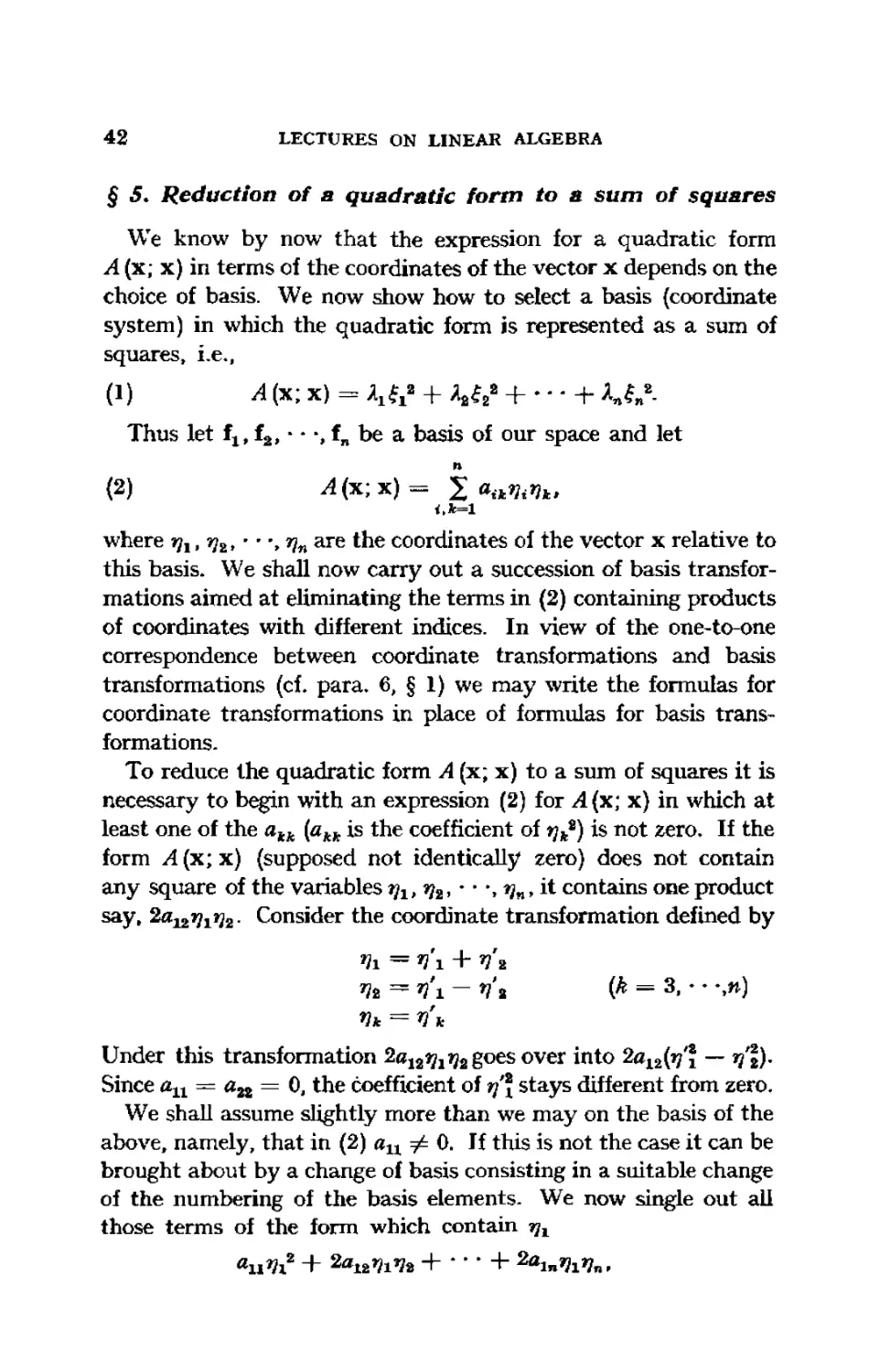
§ 5. Reduction of a quadratic form to a sum of squares
We know by now that the expression for a quadratic form
A (x; x) in terms of the coordinates of the vector χ depends on the
choice of basis. We now show how to select a basis {coordinate
system) in which the quadratic form is represented as a sum of
squares, i,e.f
(1 ) A (x; x) = XJX* + A2£2* + · - - + K^-
Thus let flf f2, ■ · ■, in be a basis of our space and let
η
{2) Λ(χ;χ)= 2 ««%**.
where ηλ, η^ · - -, ηη are the coordinates of the vector χ relative to
this basis. We shall now carry out a succession of basis
transformations aimed at eliminating the terms in (2) containing products
of coordinates with different indices. In view of the one-to-one
correspondence between coordinate transformations and basis
transformations (cf. para. 6, § 1) we may write the formulas for
coordinate transformations in place of formulas for basis
transformations-
To reduce the quadratic form A (x; x) to a sum of squares it is
necessary to begin with an expression (2) for A{x; x) in which at
least one of the akk (akk is the coefficient of η^) is not zero. If the
form A (x; x) (supposed not identically zero) does not contain
any square of the variables ητ, η2, * · ·, *}n> it contains one product
say, 2αΐ2^ι>ϊ2- Consider the coordinate transformation defined by
V* = V'i — V\ (* = 3, · · ·,»)
Under this transformation ^a12t]^2 Eoes over *п*° ^«(τ/ϊ ~~ v't)-
Since а1г = а2г = 0, the coefficient of η\ stays different from zero.
We shall assume slightly more than we may on the basis of the
above, namely, that in (2) alx Φ 0. If this is not the case it can be
brought about by a change of basis consisting in a suitable change
of the numbering of the basis elements- We now single out all
those terms of the form which contain щх

«-DIMENSION AL SPACES
43
and "complete the square," Le., write
(3) = — (Л11Ч1 + · ' ' + «ъ.4»)1 - B.
«11
It is clear that В contains only squares and products of the terms
anV2>' ' "> ainVn s0 that upon substitution of the right side of (3)
in (2) the quadratic form under consideration becomes
A (x; x) = — {апъ + · · · + ЛцЛ*)1 + ■ ■ %
where the dots stand for a sum of terms in the variables η2, · · · ηη.
If we put
4i* = «u?h + ai2^2 + ■ ' ■ + *ιη3?Λ,
4** = Пг >
then our quadratic form goes over into
1 n
Л(х; x) = — î?!*2 + Σ Ъ**Ъ*Ч***
η
The expression J aik*Vi*4k* is entirely analogous to the
i.k=2
right side of (2) except for the fact that it does not contain the
first coordinate. If we assume that α22* Φ 0 (which can be
achieved, if necessary, by auxiliary transformations discussed above)
and carry out another change of coordinates defined by
V* = Vi*>
*?2** = «22*%* + «23**73* Η + α2«**?Λ
%** = %*.
ηη** = ?Λ
our form becomes
A (x; x) = - V*2 + -Ц V + Σ *<***Vi**Vt**-
«11 »22 *.*=3

44
LECTURES ON LINEAR ALGEBRA
After a finite number of steps of the type just described our
expression will finally take the form
A <x; x) - λχξ* + λ2ξ2* +-· + ^ш\
where m ^ «.
We leave it as an exercise for the reader to write out the basis
transformation corresponding to each of the coordinate
transformations utilized in the process of reduction of A (x; x) (cf. para, 6,
§ 1) and to see that each change leads from basis to basis, i,e.t to
η linearly independent vectors.
If m < η, we put Дт+1 = ■ ■ ■ — λη = 0. We may now sum up
our conclusions as follows:
Theorem 1, Let A(n.;x) bea quadratic form in an n-dimensional
space R. Then there exists a basis elt e2, · ■ -, en of R relative to
which A {x; x) has the form
A (x; x) = Xxtf + А2г22 + · · · + ληξη\
where tlt ξ2, ■ ■ ·, ξη are the coordinates o/x relative to el3 e2> · · ·, en.
We shall now give an example illustrating the -above method of reducing
a quadratic form to a sum of squares. Thus let A (x; x) be a quadratic form
in three-dimensional space which is defined, relative to some basis fl± f2, 1г,
by the equation
A (x; x) - 2VlV2 + 4f?l4a - V - 8V-
If ·
then
Again, if
then
Finally, if
Vi — V *>
V* = v'x*
v% = v\.
Λ(χ; x) = -η\* + 2η\η\ + WtV'
Vi* = - v\ + V'%
Vi* = П'*>
η* = ν'*
Λ (χ; χ) = -4ι" + η%** ~ 4W
*1 = *Λ
£, = *.* + 2Ч»*>
S. = ?ι*.
8%

«-DIMENSIONAL SPACES
45
then A (x; x) assumes the canonical form
A (x; x) = -f !« -f- f t* - 12£3*.
If we have the expressions for ηχ*, %*, · · -, ??л* in terms of
Ъ>*1г*щлт> VnJor^**, η^**, - - % ηη** in terms of ητ*, q2*, · · -, ηη*,
etc., we can express flr f8, ■ - ·, fn in terms of ^, ^t, ■ ■·,??„ in the
form
ίΐ = Cll^l + C12^2 + ' " ' + ClnVn
£* = Стг1*?1 + C»2*?2 H + *n»4»'
Thus in the example just given
fi = Vi — V*>
£i = *7i -r 2*J*
In view of the fact that the matrix of a coordinate
transformation is the inverse of the transpose of the matrix of the
corresponding basis transformation (cf. para. 6, § I ) we can express the
new basis vectors elt e2, · · *, en in terms of the old basis vectors
ei = ^nfi + ^iaf2 H h dlnfn
e2 = d21tx + d22t2 + - ■ - + d2ntn
If the form A (x; x) is such that at no stage of the reduction
process is there need to "create squares" or to change the
numbering of the basis elements (cf. the beginning of the description of
the reduction process in this section), then the expressions for
in h> * " '» f n in terms of ηΧι η2, · ■ *, ηη take the form
fi = СцЪ + Г12*?2 + · - · + ClnVn*
Sz = С2гЧъ + " ' Ф + C2nVn>
bn Cnn Vu *
i.e. the matrix of the coordinate transformation is a so called
triangular matrix. It is easy to check that in this case the matrix

46
LECTURES ON LINEAR ALGEBRA
of the corresponding basis transformation is also a triangular
matrix:
e* = dnA + 42f2 + —Η dnntn.
§ 6. Reduction of a quadratic form by means oî a
triangular transformation
1. In this section we shall describe another method of
constructing a basis in which the quadratic form becomes a sum of squares.
In contradistinction to the preceding section we shall express the
vectors of the desired basis directly in terms of the vectors of the
initial basis. However, this time we shall find it necessary to
impose certain restrictions on the form Л (х; у) and the initial
basis ΐτ, f2> - ■ -, f„. Thus let \\aik\\ be the matrix of the bilinear
form Α (χ; у) relative to the basis flf f2, « - -, tn. We assume that
the following determinants are different from zero:
Δχ
*u
^0;
Δ* =
(1)
*11
^21
Δ« =
%x
*12
"In
*2n
7^0;
^0.
(It is worth noting that this requirement is equivalent to the
requirement that in the method of reducing a quadratic form to a
sum of squares described in § 5 the coefficients allt л22*, etc-, be
different from zero.
Now let the quadratic form A (x; x) be defined relative to the
basis flt f2> ■ · \ in by the equation
л (χ; χ) = Σ «.*£.£*> where a« = A (f.; f*)·
t,*=l
It is our aim to define vectors e1( ei? · · ·, e„ so that
(2) Λ (et-; e*) =0 for i· Φ k (i, k = 1, 2, · ■ ·, n).

«-DIMENSIONAL SPACES
47
We shall seek these vectors in the form
fn\ e2 = a2lM + a22*2'
en = ocnlfx + an2f2 + - ■ - + an„fn.
We could now determine the coefficients <xik from the conditions
(2) by substituting for each vector in (2) the expression for that
vector in (3). However, this scheme leads to equations of degree
two in the <xik and to obviate the computational difficulties involved
we adopt a different approach.
We observe that if
^(eÄ;f,) =0 for i= 1,2, ■··,*- 1,
then
A(ek; e<) = 0 for ί = 1, 2, - · ·, A - 1.
Indeed, if we replace e^ by
then
A(eft; e<) - A(ek; cc^ + ai2f2 + · · · + «„fj
= *д Л («*; fi) + afIii (e*; f2) H + a,, Л {eft; f J.
Thus if Л(еА;^) — 0 for every k and for all г < kt then
^ (ek> ei) = 0 for i < Ä and therefore, in view of the symmetry of
the bilinear form, also for г > k> i,e,, elt e2, * · ♦, e^ is the required
basis. Our problem then is to find coefficients <xfcl> aÄ2, · · ·, afcA
such that the vector
e* — a*ifi + **2f2 + ' " + *****
satisfies the relations
(4) A(et;ti)^0È <* = 1, 2, · ·-f A - 1).
We assert that conditions (4) determine the vector ek to within
a constant multiplier. To fix this multiplier we add the condition
(5) A(ek;fk) = \.
We claim that conditions (4) and (5) determine the vector eft

48
LECTURES ON LINEAR ALGEBRA
uniquely. The proof is immédiate. Substituting in (4) and (5)
the expression for ek we are led to the following linear system for
the xki:
«*i^ ft; fi) + «м^ (Ί; fa) + - - - + **И ft;f*) = °>
**iA (f»; tt) + ol^A (f2; Ц + -- + %Л (f2; f J - 0,
(6)
<**И (f* -i; fi) + «*2^ (**-ъ У + - - · + **И (f M; fk) = 0,
*klA {fk; Ϊλ) + *k2A (îk- f2) + 1- *kkA (fÄ; tk) = 1.
The determinant of this system is equal to
Ij-ifo-y ift.f.) --- ^(fi;ffc)|
(7) zifc = r^:fl) л('гЛ) '" yl(f*;f*M
and is by assumption (1) different from zero so that the system (6)
has a unique solution. Thus conditions (4) and (5) determine ek
uniquely, as asserted.
It remains to find the coefficients bik of the quadratic form
A (x; x) relative to the basis elf e2i ■ · -, ея just constructed. As
we already know
bik = А(е,;ек).
The basis of the e{ is characterized by the fact that A (e<; ek) — 0
for г -f- к, i.e., bik = 0 f or ι'Φ L· It therefore remains to compute
bkk = A(ektek). Now
Л(еА; eA) = Л(еА; α^ + aÄ2f2 -i + ajM!f*)
- aklA (ek> fx) + a*2A (efc; f2) + « « « + %4 (e^ f*)>
which in view of (4) and (5) is the same as
The number <хкк can be found from the system (6). Namely, by
Cramer's rule,
*-" л ·
where ^к_х is a determinant of order к — 1 analogous to (7) and

«-DIMENSIONAL SPACES
49
Thus
bkk = A{ej£;ek) =
JA-1
To sum up:
Theorem 1, Let Α {κ; χ) be a quadratic form defined relative to
some basis fx> f2> · · -, fn by the equation
η
A (x; x) = X aikViVk. «a = A (ft> f*)·
Further, let the determinants
Δχ = at
Δ9 =
*n
Δ„ =
*21
*7ϊ1 "τι2
fo д# different from zero. Then there exists a basis ex, e2, ■
relative to which A {x; x) zs expressed as a sum of squares,
An A* A„ t
A (x; x) = -^ V + -^ ft« + - · · + -^ f„2
Л*+ -*·*+
/tere fi, Î2* * β β» fn ar,ß ^ coordinates of χ râ /Лг -basis ex, e2, · · ·, en.
This method of reducing a quadratic form to a sum of squares is
known as the method of Jacobi,
Remark: The fact that in the proof of the above theorem we
were led to a definite basis ex> e2, * · ·, e„ in which the quadratic
form is expressed as a sum of squares does not mean that this basis
is unique. In fact, if one were to start out with another basis
f^fa, · * ·, fw (or if one were simply to permute the vectors f2,
f2, ■ · -, fj one would be led to another basis ex> e2, —, en.
Also, it should be pointed out that the vectors €x, e2,
not have the form (3),
Example. Consider the quadratic form
4S + 3|t f, + 4*^ + ξ^ + ξ S
in three-dimensional space with basis
U - (1, 0, 0). ft = (0, IP 0), fa - № 0, 1).
, e^ need

50
LECTURES ON LINEAR ALGEBRA
The corresponding bilinear form is
A (x; y) - 2ξιηι -f |flî?s -f- 2£li3a -f- f Mi + it* + 2sVh - f8*.
The determinants z^, d2, ^sare 2, —^. — ^, Le., none οί them vanishes.
Thus our theorem may be applied to the quadratic form at hand. Let
«1 ~ «11*1 - («ll»0' °)-
e» = ctaifx H- aMft + aMf8 = (a31f αω, αΜ).
The coefficient au is found from the condition
i.e., 2an = 1, or stn = £ and
*i - fr = (i 0, 0).
Next asl and «as are determined from the equations
Л (е.; fj = 0 and Л (eÎP f,) = 1.
or,
whence
and
2aai + |a„ - 0; f aai + aM - 1.
*« — 6, a„ = -8,
es = 6f\ - 8iu = (6. -8, 0).
Finally, aai, a„, азэ are determined from the equations
A {e,; ft) = 0, A (e,; f,) =0, A (es; f8) = 1
or
2аи -f ■§ aat -r 2a8a = 0.
whence
and
+ «S3 = h
ρ _ 8 f 12f , 1 f _ / 8 12 1 ч
Relative to the basis elf etf ea our quadratic form becomes
Α (χ; χ) = i С/ + ^ C.m + χ С.1 = 4 Îia - *?»* + J-ί Д
Jj /Jm Ла A'
Неге flt С·, t* Are the coordinates of the vector χ in the basis e^ e», ea.

n-DIMENSIONAL SPACES 51
2, In proving Theorem 1 above we not only constructed a basis
in which the given quadratic form is expressed as a sum of squares
but we also obtained expressions for the coefficients that go with
these squares. These coefficients are
J_ ^1 ... ^=λ
Аг' Δ2' Δη
so that the quadratic form is
<8> i('* + b''+--- + dAS''-
It is clear that if Ai_1 and Ai have the same sign then the coefficient
of ξ{2 is positive and that if A^ and Ai have opposite signs, then
this coefficient is negative. Hence,
Theorem 2. The number of negative coefficients which appear in
the canonical form (8) of a quadratic form is equal to the number of
changes of sign in the sequence
1>Лг,Аг, ■ ■ ;Δη.
Actually, all we have shown is how to compute the number of
positive and negative squares for a particular mode of reducing a
quadratic form to a sum of squares. In the next section we shall
show that the number of positive and negative squares is
independent of the method used in reducing the form to a sum of squares.
Assume that ^t > 0, A2> 0, · · ·, zln > 0. Then there exists a
basis ex, e2, ■ · -, e„ in which A (x; x) takes the form
Л (x; x) = Ajfi» + Д2£22 + · · - + ληξη\
where all the Λ, are positive. Hence A (x; x) Й 0 for all χ and
Λ(χ;χ) = J Α,-ί,-^Ο
is equivalent to
it = f. = ■ · · -= f „ = o.
In other words,
If Аг > 0, A2 > 0, · · -, An > 0, then the quadratic form A (x; x)
is positive definite.

52
LECTURES ON LINEAR ALGEBRA
Conversely, let A (x; x) be a positive definite quadratic form.
We shall show that then
Ak > 0 (k = 1, 2, - - -, n).
We first disprove the possibility that
U^fj A(ilff2) ·-- A(fltfk)
Ak =
^(f^fj ^(fft;f2)
^(f*;«*)i
If 4Ä — о, then one of the rows in the above determinant would be
a linear combination of the remaining rows, i.e., it would be
possible to find numbers μΐ9 μ2, · · -, μ* not all zero such that
μΎΑ ft; ÎJ + μ2Α ft; fJ + · · - + μ,Α (tk; f J - 0,
ΐ — 1, 2, — ·, Λ. But then
Л(/<А + jK8f2 + ■ ■ ■ + /*A; fi) = o (t == if sf · · ·, *)f
so that
Α \μ& + μΑ + ' ' · + /Ά; Mi + /Ά + " " " + /*A) = °-
Γη view of the fact that μ^ + μΑ + · - ■ + μΑ ~i~ °* the latter
equality is incompatible with the assumed positive definite nature
of our form.
.The fact that Ak Φ 0 (к = 1, · · ·, «) combined with Theorem 1
permits us to conclude that it is possible to express A (x; x) in the
form
A (x; x) = W + W + - - - + hL2> К
Jfc- 1
Since for a positive definite quadratic form all Ак > О, it follows
that all Ak > 0 (we recall that A0 — 1).
We have thus proved
Theokem 3. Let A (x; y) be a symmetric bilinear form and
tx> f2, - - -, tn> a basis of the η-dimensional space R. For the quadratic
form A (x; x) to be positive definite it is necessary and sufficient that
Δχ > 0, A2 > 0, - · ·, An > 0.
This theorem is known as the Sylvester criterion for a quadratic
form to be positive definite.

^-DIMENSIONAL SPACES
53
It is clear that we could use an arbitrary basis of R to express the
conditions for the positive definiteîiess of the form Α (χ; χ). Τη particular
if we used аь another basis the vectors iit f2, * * -, fK in changed order, then
the new Alt A2l ■ - -, An would be different principal minors of the matrix
||oft||. This implies the following interesting
Corollary, If the principal minors Alr A2, ■ · ·, Anof a matrix \\aJk\\ of a
quadratic form A (x; x) relative to some basis are positive, then all principal
minors of that matrix are positive.
Indeed, if At, A2, · ■ -, An are all positive, then A (x, x) is positive definite.
Now let A be a principal minor of \\alk\\ and let pz „ p2r - ■ -, pk be the
numbers of the rows and columns of |[aik' | in Δ. If we permute the original basis
vectors so that the ptth vector occupies the ith position {i — \, · ■ ·, k) and
express the conditions for positive definiteness of A (x; x) relative to the new
basis, we see that Δ > 0.
3, The Gramm determinant. The results of this section are valid
for quadratic forms A (x; x) derivable from inner products, i.e.,
for quadratic forms A (x; x) such that
^(x;x) = (x,x).
If A {x; y) is a symmetric bilinear form on a vector space R and
A (x; x) is positive definite, then A (x; y) can be taken as an inner
product in R, i.e., we may put (x, y) =ξ= Л {x; y). Conversely, if
(x, y) is an inner product on R, then A (x; y) ξ (χ, у) is a bilinear
symmetric form on R such that A (x; x) is positive definite. Thus
every positive definite quadratic form on R may be identified with
an inner product on R considered for pairs of equal vectors only,
A (x; x) = (x, x). One consequence of this correspondence is that
every theorem concerning positive definite quadratic forms is at
the same time a theorem about vectors in Euclidean space.
Let ex, e2, ■ ■ -, ek be к vectors in some Euclidean space. The
determinant
|{elfex) (e^e,) --- (elfefc)|
{e^ej (e2,e2) -■■ (e2, ek)\
|(e*,Êi) (e*,e2) -■ (ek>ek)\
is known as the Gramm determinant of these vectors.
Theorem 4. The Gramm determinant of a system of vectors
ex> e2, - - \ efc is always È 0- This determinant is zero if and only if
the vectors el$ e2> - - -, ek are linearly dependent.

54
LECTURES ON LINEAR ALGEBRA
4.=
Proof: Assume that eltez, ♦ * ·, ek are linearly independent.
Consider the bilinear form A (x; y) = (x, y), where (x, y) is the
inner product of χ and y. Then the Gramm determinant of
ei> e2; * * "* eJt coincides with the determinant Ak discussed in this
section {cf. (7)). Since A (x; y) is a symmetric bilinear form such
that A(x; x) is positive definite it follows from Theorem 3 that
Jk>0.
We shall show that the Gramm determinant of a system of
linearly dependent vectors el7 ea, ■ ■ -, ek is zero. Indeed, in that
case one of the vectors, say eA, is a linear combination of the others,
e* = *iei + A2e2 H h ^ι**-ι·
It follows that the last row in the Gramm determinant of the
vectors el7 e2, - · ·, eA is a linear combination of the others and the
determinant must vanish. This completes the proof.
As an example consider the Gramm determinant of two vectors
χ and y
{χ, χ) (χ, y) Ι
(У. x) (У> У) I
The assertion that Δ2 > 0 is synonymous with the Schwarz
inequality.
Examples. 1. In Euclidean three-space (or in the plane) the determinant
^j'has the following geometric sense: Δ% is the square of the area of the
parallelogram with sides X and y. Indeed,
(χ, y) = (y> χ) = |χ| * |y| cos Ψί
where ψ is the angle between x and y. Therefore,
Δχ = [X|a |у|» - |x|* |У|2 cos« φ = |x[* |y|» (1 - cos* <p) = |x|» [y|· sin* φ.
i.e., Δ% has indeed the asserted geometric meaning.
2, In three-dimensional Euclidean space the volume of a parallelepiped
on the vectors x, y, z is equal to the absolute value of the determinant
iCj Jtjj X3
Vi У* У*
zx гг ζ*
where x(t yit zM are the Cartesian coordinates of x± y, z. Now,
*i2 -f a?22 + x** a^Vt + я*У* Η" **У* a-i*i -r Яг*г -f ss;?8
2/i*i + У*хг + У**г У ι2 + Уг* + Уг* у7гг + у%х% + у%х%
*ι*ι + х*х* + *■*» *ι2/ι + **У* + *»У* V + */ 4- V

«-DIMENSIONAL SPACES
55
| (χ, χ) (χ, y) (x, z) 1
(У- Ό (У> У) (У. »)
(z. x) (z, y) (z, z) j
Thus the Gramm determinant of three vectors x,
volume of the parallelepiped on these vectors.
Similarly, it is possible to show that the Gramm determinant of k vectors
x, У, * * -P w in a Ä-dimenional space R is the square of the determinant
, y, z is the square of the
O)
Vi У*
У*
where the xf are coordinates of χ in some orthogonal basis, the yt are the
coordinates oi у in that basis, etc.
(It is clear that the space R need not be ^-dimensional, R may, indeed,
be even infinite-dimensional since our considerations involve only the
subspace generated by the к vectors x, y, ■ * -, w. )
By analogy with the three-dimensional case, the determinant (9) is
referred to as the volume of the ^-dimensional parallelepiped determined by
the vectors x, y, · - ·*, w.
3. In the space of functions (Example 4, § 2) the Gramm determinant
takes the form
Г/,*(')<*' f'/iM/.M* · ■ f*/i(0/.W*
Ja Ja Ja
Γ/ιΜ/ι(0ώ ['/.»(Ο* ■■· Γ*/,(/)/,(t)dt
Ja Ja Ja
Ja Ja Ja
and the theorem just proved implies that:
The Gramm determinant of a system of functions is always ^ 0. For a
system of functions to be linearly dependent it is necessary and sufficient that
their Gramm determinant vanish.
§ 7. The inw of inertia
1« The law of inertia. There are different bases relative to
which a quadratic form A (x; x) is a sum of squares,
(I)
Λ(χ;χ)=ΣΛ^·
t=I
By replacing those basis vectors (in such a basis) which
correspond to the non-zero Λ, by vectors proportional to them we obtain a

56
LECTURES ON LINEAR ALGEBRA
representation of A (x; x) by means of a sum of squares in which
the A, arc 0t 1, or — 1. It is natural to ask whether the number of
coefficients whose values are respectively 0, 1, and—1 is dependent
on the choice of basis or is solely dependent on the quadratic
form A (x; x).
To illustrate the nature of the question consider a quadratic
form ^4(x;x) which, relative to some basis e^e^*--, enI is
represented by the matrix
iktii.
where atk = A (ef; ek) and all the determinants
A — а Л — Γ11 *1SS I
I "21 "22 I
\aU «12 '" «Inj
\a21 a22 · ■ ■ a2n
are different from zero. Then, as was shown in para. 2, § 6, all ^
in formula (1) are different from zero and the number of positive
coefficients obtained after reduction of A (x; x) to a sum of squares
by the method described in that section is equal to the number of
changes of sign in the sequence l,Altà2,-tm,àn*
Now, suppose some other basis e\, e'2, · - % e'w were chosen.
Then a certain matrix ||-a'£J| would take the place of \\aik\\ and
certain determinants
would replace the determinants Alt Δ2, · · ·, Δη. There arises the
question of the connection (if any) between the number of changes
of sign in the squences 1, Δ\,Δ\> · · -, Δ'η and 1, Δΐ9 Δ^, · * ·, Δη.
The following theorem, known as the law of inertia of quadratic
forms, answers the question just raised-
Theorem 1. If a quadratic form is reduced by two different
methods (i.e., in two different bases) to a sum of squares, then the
number of positive coefficients as well as the number of negative
coefficients is the same in both cases.

W-DIMENSIONAL SPACES 57
Theorem 1 states that the number of positive Я4 in (1) and the
number of negative λζ in (1) are invariants of the quadratic form.
Since the total number of the Λ,- is n> it follows that the number of
coefficients λί which vanish is also an invariant of the form.
We first prove the following lemma:
Lemma. Let R' and R" be two subspaces of an n-dimensional
space R of dimension k and /, respectively, and let k + / > n. Then
there exists a vector x^O contained in R' η R".
Proof: Let elr e2, · ■ -, et be a basis of R' and fx> f2, - - ·, ft,
basis of R"* The vectors elt e2, - · -, ekt flf f2> · * -, fj are linearly
dependent (k + / > n). This means that there exist numbers
Αι* A2, ■ ■ -, AÄJ μχ, μ2, я - \ μι not all zero such that
Atex + A2e2 Η + Акек + μιίΎ + μ212 Η + Λί, = 0,
i.e.,
^iei + А2е2 4 h *fceÄ = — Μι — μ2ί2 — /^f*.
Let us put
*iei + A2e2 + · · · + ЯлеА = — μ^ — //2f2 — · · · — μ& = χ.
It is clear that χ is in R' η R". It remains to show that x^O.
If χ = 0, λλ, λ2, - * ·, ЯА and μχ, ju2, « « ·, ^ would all be zero, which
is impossible- Hence χ ^ 0.
We can now prove Theorem 1.
Proof: Let elf e2, - · -, ея be a basis in which the quadratic form
i4{x; x) becomes
(2) A{x; x) = V + f22 + ■- - + fp* - f%+1 - fV2 «W
(Here fi,f2.e·-, fn are r^e coordinates of the vector x, Le.,
x = f^ + f2e2 + - · · + Mp + ίΐΗ-ιβ,+ι + h 1иЛ-нг + "β '
+fnen.) Let flf f2, ■ -, fn be another basis relative to which the
quadratic form becomes
(3) A (x; x) = 4l· + %« + ■ - . + ГД, _ ,2^+1 _ ,ι^ ,
(Here jjlt ??2> · ■ -, ηη are the coordinates of χ relative to the basis
flt f2t · · ·, f„.) We must show that p = P' and g = qf. Assume
that this is false and that ρ > p\ say.
Let R' be the subspace spanned by the vectors eb e2, ■ * ·, ер.

58
LECTURES ON LINEAR ALGEBRA
R' has dimension p. The subspace R" spanned by the vectors
V+i· V+2* ' * '* Ίι nas dimension η — p'. Since η — ρ' + ρ > η
(we assumed p > p'), there exists a vector χ ^ 0 in R' η R"
(cf. Lemma), Le.,
x = £i*i + f2e2 H + f*e*
and
The coordinates of the vector χ relative to the basis ex, e2, · · ·, ея
are fi, f8, · · % fpf 0t · · % 0 and its coordinates relative to the basis
Ί» '21# * *» fn are **> *-*, · ' "* °» ^»'+1» ' ' *> 4«· Substituting these
coordinates in (2) and (3) respectively we get, on the one hand,
(4) Л(х; x) - V + f,2 + - - · + f,1 > 0
(since not all the f, vanish) and, on the other hand,
(5) A <x; X) - - 4V+1 - 4V+i 4V^ ^ 0.
(Note that it is not possible to replace g in (5) with <, for, while
not all the numbers η^+1,*ΛΛ,ηη are zero, it is possible that
V*'+i — ^+2= л ' ^ = Vv'+q' — 0.) The resulting contradiction
shows that p — p\ Similarly one can show that q — g\ This
completes the proof of the law of inertia of quadratic forms.
2. Rank of a quadratic form
Definition L By the tank of a quadratic form we mean the
number of non-zero coefficients Хг in one of its canonical forms.
The reasonableness of the above definition follows from the law
of inertia just proved. We shall now investigate the problem of
actually finding the rank of a quadratic form. To this end we
shall define the rank of a quadratic form without recourse to its
canonical form.
Definition 2. By the null space of a given bilinear form А (х; у)
we mean the set R0 of all vectors у such that A (x; у) = О for every
xeR.
It is easy to see that R0 is a subspace of R, Indeed, let y2,
yfi e R0> Le-, A (x; yx) = О and A (x; ya) = 0 for all χ e R. Then
A (x; yj + y8) = 0 and A (x; Лух) = 0 for all χ e R. But this
means that yx + y2 e R0 and Дух е R0.

«-DIMENSIONAL SPACES
59
We shall now try to get a better insight into the space R0.
If fx> f2> —, fn is a basis of R, then for a vector
(в) У = vA + ηΑ Η l· vA
to belong to the null space of A (x; y) it suffices that
(7) A(tt;y) = 0 for t=lt2f---t«.
Replacing у in (7) by (6) we obtain the following system of
equations:
A (fi; *lA + nA + ·- + ηηΐη) - 0,
A (**'> ПА + ^2f2 Η l· VnK) = °>
MU\ vA + vA + · · ' + чА) = °-
If we put ^(ft-;fÄ) = aik> the above system goes over into
«n^i + ai2*?2 Η l· «in7?« = °>
Thus the null space R<, consists of all vectors y whose coordinates
4ι ι Цъ> ' ' "» ^n are solutions of the above system of linear equations.
As is well known, the dimension of this subspace is η — r, where r
is the rank of the matrix \\aik\\.
We can now argue that
The rank of the matrix \\atk\\ of the bilinear form A (x; y) is
independent of the choice of basis in R (although the matrix \\aik\\
does depend on the choice of basis; cf. § 5).
Indeed, the rank of the matrix in question is η — r0, where r0
is the dimension of the null space, and the null space is completely
independent of the choice of basis.
We shall now connect the rank of the matrix of a quadratic
form with the rank of the quadratic form. We defined the rank
of a quadratic form to be the number of (non-zero) squares in any
of its canonical forms. But relative to a canonical basis the matrix
of a quadratic form is diagonal
α о ■·· on
о л2 - · · о
Lo о .·· я J

60
LECTURES ON LINEAR ALGEBRA
and its rank r is equal to the number of non-zero coefficients, i.e.,
the rank of the quadratic form. Since we have shown that the
rank of the matrix of a quadratic form does not depend on the
choice of basis, the rank of the matrix associated with a quadratic
form in any basis is the same as the rank of the quadratic form. б
To sum up:
Theorem 2. The matrices which represent a quadratic form in
different coordinate systems all have the same rank r. This rank is
equal to the number of squares with non-zero multipliers in any
canonical form of the quadratic form.
Thus, to find the rank of a quadratic form we must compute
the rank of its matrix relative to an arbitrary basis.
§ 8. Complex η-dimensional space
In the preceding sections we dealt essentially with vector spaces
over the field of real numbers. Many of the results presented so
far remain in force for vector spaces over arbitrary fields. In
addition to vector spaces over the field of real numbers, vector
spaces over the field of complex numbers will play a particularly
important role in the sequel. It is therefore reasonable to discuss
the contents of the preceding sections with this case in mind.
1. Complex vector spaces. We mentioned in § 1 that all of the
results presented in that section apply to vector spaces over
arbitrary fields and, in particular, to vector spaces over the field
of complex numbers.
2. Complex Euclidean vector spaces. By a complex Euclidean
vector space we mean a complex vector space in which there is
defined an inner product, i.e., a function which associates with
every pair of vectors χ and у a complex number (x, y) so that the
following axioms hold:
1. (χ, y) = (y, χ) [(yf χ) denotes the complex conjugate of
(y,x)];
6 We could have obtained the same result by making use of the well-
known fact that the rank of a matrix is not changed if we multiply it by
any non-singular matrix and by noting that the connection between two
matrices si and jai which represent the same quadratic form relative to two
different bases is J - Vf' j/tf, <€ non^singular.

«-DIMENSIONAL SPACES
6]
2. (Ях,у) = /(Хру);
3. (хг + x2, у) = (Xl, у) + (χ2, у);
4. (χ, χ) is a non-negative real number which becomes zero
only if χ = 0.
Complex Euclidean vector spaces are referred to as unitary
spaces.
Axioms 1 and 2 imply that (x, Ay) — Цх, у). In fact,
(x> *y) = (*У, x) = %, x) = Л(х, у).
Also, {χ, уг + y2) = (χ, yx) + (x, y2). Indeed,
(x, Ух + У2) = (Ух + Y*, x) = (Yi, x) + (У2. x) = (x.Ух) + (x,У*)·
Axiom 1 above differs from the corresponding Axiom 1 fora real Euclidean
vector space. This is justified by the fact that in unitary spaces it is not
possible to retain Axioms 1, 2 and 4 for inner products in the form in which
they are stated for real Euclidean vector spaces, indeed,
[χ* y) = (y, χ).
would imply
(xr;.y) = Д(х,у).
But then
(Дх. Дх) - Λ2(x, x).
In particular,
(ix, ix) = — (χ, χ),
i.e., the numbers (χ, χ) and (у, у) with у = гх would have different signs
thus violating Axiom 4
Examples of unitary spaces. 1, Let R be the set of «-tuples
of complex numbers with the usual definitions of addition and
multiplications by (complex) numbers. If
x = (lit £2, * ' \ £») and у = (Vl, η2ι « « -, Vn)
are two elements of R, we define
(x, y) - ^17, + ξ2ή2 + · · · + ξηήη.
We leave to the reader the verification of the fact that with the
above definition of inner product R becomes a unitary space.
2. The set R of Example 1 above can be made into a unitary
space by putting
(χ. у) = 1 ợ л*.

62
LECTURES ON LINEAR ALGEBRA
where aik are given complex numbers satisfying the following two
conditions:
(a) aik = aki
(β) Υ aikSt I* Й 0 for every «-tuple ξΐ9 ξ2, - · \ ξη and takes on
the value zero only if ξx = ξ2 = ■ - ■ = ξη = 0,
3. Let R be the set of complex valued functions of a real
variable i defined and integrabie on an interval [a, b\ It is easy to
see that R becomes a unitary space if we put
{/(t),g{t))=fa/(t)W)dt·
By the length of a vector χ in a unitary space we shall mean the
number \/(x, x). Axiom 4. implies that the length of a vector is
non-negative and is equal to zero only if the vector is the zero
vector.
Two vectors χ and y are said to be orthogonal if (x, y) = 0.
Since the inner product of two vectors is, in general, not a real
number, we do not introduce the concept of angle between two
vectors.
3. Orthogonal basis. Isomorphism of unitary spaces. By an
orthogonal basis in an и-dimensionai unitary space we mean a set
of η pairwise orthogonal non-zero vectors elf e2, · · ·, en. As in § 3
we prove that the vectors е1,е2,-1',еп are linearly independent,
i.e., that they form a basis.
The existence of an orthogonal basis in an «-dimensional unitary
space is demonstrated by means of a procedure analogous to the
orthogonalization procedure described in § 3.
И -©i, e2, * ' ', ■£« is an orthonormal basis and
x = ξ^ι + £2e2 + h ϊη*η, У = V^i + П**2 + h ηη*η
are two vectors, then
(x, y) = (f xe£ + f2e2 + h ?nen, V& + >?2e2 + h *?new)
= f Ä + hv* H + f«tf»
(cf. Example 1 in this section)-
If ©i. e2> * * '*e« is an orthonormal basis and
x = fxei + fae2 + ·"'■ + (nen>

«-DIMENSIONAL SPACES
63
then
(x, e£) = (ίΛ + £2e2 + h £,ея, ej = ξχ(*τ, ej
+ ?2(ег,е,) + ·■■ + *„(««>««).
so that
(x,e<) = f,.
Using the method of § 3 we prove that all unitary spaces of
dimension η are isomorphic.
4. Bilinear and quadratic forms. With the exception of positive
definiteness all the concepts introduced in § 4 retain meaning for
vector spaces over arbitrary fields and in particular for complex
vector spaces. However, in the case of complex vector spaces
there is another and for us more important way of introducing
these concepts.
Linear functions of the first and second kind. A complex valued
function/defined on a complex space is said to be a linear function
of the first kind if
1. /(x -f- y) =/(x) +/(y).
2. /(Ях) = A/(x),
and a linear function of the second kind if
i. /(x + y)=/(x)+/(y).
2. /μχ) = λ/(χ).
Using the method of § 4 one can prove that every linear function
of the first kind can be written in the form
/(x) = α1ξ1 + α2ξ2 + · · · + αηξη>
where ξ{ are the coordinates of the vector χ relative to the basis
*t> β2ί--', en and at are constants, a, = /(e£), and that every
linear function of the second kind can be written in the form
f(x)^bjx+bj2+--+bjn.
Definition 1, We shall say that A (x; y) is a bilinear form
(function) of the vectors χ and у if:
1. for any fixed y, A (x; y) is a linear function of the first kind o/x,
2« for any fixed X, A (x; y) is a linear function of the second kind
of y. In other words,
1. A{Xi + x2;y) ^Л(Х1;у) +Л(х2;у),
Л(Дх;у) = АЛ(х;у),

64
LECTURES ON LINEAR ALGEBRA
2. A (x; y2 + y3) = A <x; yt) + A (x; y2),
Л(х;Ау) = Ы{к;у).
One example of a bilinear form is the inner product in a unitary
space
A (x; y) = (x, y)
considered as a function of the vectors χ and y. Another example
is the expression
η
Л(х;у)= Σ ««Μ*
viewed as a function of the vectors
У = №l + 3?2e2 + ' " + Vn^n-
Let elt e2, —, en be a basis of an «dimensional complex space.
Let A (x; y) be a bilinear form. If χ and у have the representations
x => fi^i + f2e2 Η l· *·©«, У = чЛ + i?2e2 + h ηη*«>
then
Л (χ; у) = Α (ξ^ + f2e2 + · - - fnen; %ех + %е2 Η + ^е„)
η
The matrix ||aifc|| with
л1А = ^(e£;efc)
is called the matrix of ike bilinear form A (x; y) relative to the basis
ei» ea* " " "» en*
If we put у = χ in a bilinear form A (x; y) we obtain a function
Л(х; x) called a quadratic form (in complex space). The
connection between bilinear and quadratic forms in complex space is
summed up in the following theorem:
Every bilinear form is uniquely determined by its quadratic
form. 6
fl We recall that in the case of real vector spaces an analogous statement
holds only for symmetric bilinear forms (cf. § 4),

«-DIMENSIONAL SPACES
65
Proof: Let A (x; x) be a quadratic form and let χ and y be two
arbitrary vectors. The four identities7:
(I) A (x+y; x+y) = A (x; x) + A (y; x) + A (x; y) + A (y; y),
(II) A(x+iy; х+*у)=Л(х; x)+iA(y; *)-iA(x; у)+Л(у; у),
(III) A(x-y;x-y) = A(x;x)-A(y;x)-A{x:y)+A(y;y)>
(IV) A{x-iy; x-iy)=A(x; x)-iA(y; x)+iA{x; y)+A(y; y),
enable us to compute Л{х;у). Namely, if we multiply the
equations (I), (II), (III), (IV) by 1, i, — 1, — -*, respectively,
and add the results it follows easily that
(1) A(x; y) = l{A(x + y; χ + y) + iA (x + iy; x + iy)
— A (x - y; χ — y) — iA (x — iy; χ - iy)}.
Since the right side of (I) involves only the values of the quadratic
form associated with the bilinear form under consideration our
assertion is proved.
If we multiply equations (1), (II), (III), (IV) by 1, — i, — 1, i,
respectivly, we obtain similarly,
(2) A(y; x) = \{A(x + y; χ + у) - iA(x + iy; χ + iy)
— A (x - y; χ - y) + iA (x — iy; χ - iy)}.
Definition 2. A bilinear form is called Hermiiian if
A(x;y) =A{y;x).
This concept is the analog of a symmetric bilinear form in a real
Euclidean vector space.
For a form to be Hermitian it is necessary and sufficient that its
matrix ||öifc[| relative to some basis satisfy the condition
ai* = äki-
Indeed, if the form A (x; y) is Hermitian, then
*,* = 4(ef; e,) = ~A (efc; e<) = аы.
Conversely, if aik = äki, then
^(x;y) = Σ ««*<** = 2«*^Д^^(у;х)-
Note: If the matrix of a bilinear form satisfies the condition
* Note that A (x; Ay) = ÄA (x, y), so that, in particular, A{x.;iy)
= ^L4(x;y),

66
LECTURES ON LINEAR ALGEBRA
aik = àki, then the same must be true for the matrix of this form
relative to any other basis. Indeed, aik — dki relative to some basis
implies that A (x; y) is a Hermitian bilinear form; but then aik=äki
relative to any other basis.
If a bilinear form is Hermitian, then the associated quadratic
form is also called Hermitian. The following result holds:
For a bilinear form Л(х; у) to be Hermitian it is necessary
and sufficient that A (x; x) be real for every vector x.
Proof: Let the form A(x;y) be Hermitian; i.e., let Л(х;у)
= A (y; x). Then A {x; x) — A (x; x), so that the number
Л{х; χ) is real. Conversely, if A {x; x) is real for al x, then, in
particular, A (x + y; χ + у), Α (χ + ay; χ + iy), A {x — y; x-y),
A (x — t'y; x — iy) are all real and it is easy to see from formulas
(1) and (2) that Л(х;у) =Ä(y;x).
Corollary. A quadratic form is Hermitian if and only if it is real
valued.
The proof is a direct consequence of the fact just proved that for
a bilinear form to be Hermitian it is necessary and sufficient that
A (x; x) be real for all x.
One example of a Hermitian quadratic form is the form
Л(х;х) = (χ, χ),
where (χ, χ) denotes the inner product of χ with itself. In fact,
axioms 1 through 3 for the inner product in a complex Euclidean
space say in effect that (x, y) is a Hermitian bilinear form so that
(x, x) is a Hermitian quadratic form.
If, as in § 4, we call a quadratic form A {x; x) positive definite
when
A (x; x) > 0 for χ φ 0,
then a complex Euclidean space can be defined as a complex
vector space with a positive definite Hermitian quadratic form.
If si is the matrix of a bilinear form A (x; y) relative to the
basis er, e2> ■ · ·, en and Ш the matrix of A(x; y) relative to the
η
basis flt f3, ■ · ·, fn and if f, = £ i^e, (j = 1, · · ·, n), then

«-DIMENSIONAL SPACES
67
Here # = ||ctiJ| and ^* = \)c*^\\ is the conjugate transpose of #,
i.e., c*u = c„.
The proof is the same as the proof of the analogous fact in a real
space.
5. Reduction of a quadratic form to a sum of squares
Theokem 1. Let A (x; x) be a Hermitian quadratic form in a
complex vector space R. Then there is a basis elf e2, * * \ en of R
relative to which the form in question is given by
A (x; x) - A^ + W2 + - · ■ + XJJnt
where all the ?Js are real.
One can prove the above by imitating the proof in § 5 of the
analogous theorem in a real space. We choose to give a version of
the proof which emphasizes the geometry of the situation. The
idea is to select in succession the vectors of the desired basis.
We,choose e2 so that А (ег; ег) Ф 0. This can be done for
otherwise A (x; x) = 0 for all χ and, in view of formula (1), A (x; y) = 0.
Now we select a vector e2 in the {n — 1)-dimensional space R(1>
consisting of all vectors χ for which ^4{ег;х) = 0 so that
A(e2, e2) Φ 0, etc. This process is continued until we reach the
space R(r) in which A (x; у) == О (Rfr> may consist of the zero
vector only). If Rlr) Φ 0, then we choose in it some basis er+1,
er+2* " " "- en- These vectors and the vectors е1л e2, - · -, er form a
basis of R.
Our construction implies
-4 (e<; efc) = 0 for г < k.
On the other hand, the Hermitian nature of the form ^4(x;y)
implies
Л(е<; ек) ~ 0 for i > k.
It follows that if
x = fi^i + f2e2 + ■ · · + ёпеп
is an arbitrary vector, then
A (x; xl = ξ J, A (ei; ег) + ξ2ξ2Α (e2; e2) + · · - + ξηξηΑ (en; e„),
where the numbers A (eit e^) are real in view of the Hermitian

68
LECTURES ON LINEAR ALGEBRA
nature of the quadratic form. If we denote А(ег] ej by Xiy then
A (x; x) = XJJ± + A2f2f2 + - - - + XJJn = Xtftf + Л2||а|*
+ · · · + K\U2-
6. Reduction of a Hermittan quadratic form to a sum of squares
by means of a triangular transformation. Let A (x; x) be a Hermitian
quadratic form in a complex vector space and e1;e2,*",en a
basis. We assume that the determinants
Δχ = allt A
2
*11 "12
^21 ^2?
4. = ,
«II «IS
j Я21 а22
nl **л2
where Äift — А (е<; ек), are all different from zero. Then just as in
§ 6, we can write down formulas for finding a basis relative to
which the quadratic form is represented by a sum of squares.
These formulas are identical with (3) and (6) of § 6. Relative to
such a basis the quadratic form is given by
A <x; x) = ^ IfJ« + ^ № + ■ ■ · + ^p-1 l£J2.
where ΔΌ = 1. This implies, among others, that the determinants
Δΐ9Δ2, · · ·,Δη are real. To see this we recall that if a Hermitian
quadratic form is reduced to the canonical form (3)T then the
coefficients are equal to A (e,; ег) and are thus reaL
Exercise Prove directly that if the quadratic form A (x; x) is Hermitian,
then the determinants Δ9,Δ19 - m -, Δη are real.
Just as in § 6 we find that for a Hermitian quadratic form to be
positive definite it is necessary and sufficient that the determinants
Alt Δ2, · * % Δη be positive.
The number of negative multipliers of the squares in the canonical
form of a Hermitian quadratic form equals the number of changes of
sign in the sequence
1,Δ19Δ2, - · -,JR.
7. The law of inertia
Theorem 2. // a Hermittan quadratic form has canonical form

«-DIMENSIONAL SPACES
69
relative to two bases, then the number of positive, negative and zero
coefficients is the same in both cases.
The proof of this theorem is the same as the proof of the
corresponding theorem in § 7.
The concept of rank of a quadratic form introduced in § 7 for real
spaces can be extended without change to complex spaces.

CHAPTER II
Linear Transformations
§ 9. Linear transformations. Operations on linear
transformations
1. Fundamental definitions. In the preceding chapter we
studied functions which associate numbers with points in an n-
dimensional vector space. In many cases, however, it is necessary
to consider functions which associate points of a vector space with
points of that same vector space. The simplest functions of this
type are linear transformations.
Definition 1. J/ with every vector χ of a vector space R there is
associated a [unique) vector y in R, then the mapping y = A(x) is
called a transformation of the space R.
This transformation is said to be linear if the following two
conditions hold:
1. A(xx + x2) = A(xx) + A(x2),
2. Α(Λχ) = ΛΑ (χ).
Whenever there is no danger of confusion the symbol A(x) is
replaced by the symbol Ax,
Examples. 1ψ Consider a rotation of three-dimensional
Euclidean space R about an axis through the origin. If χ is any vector
in RT then Ax stands for the vector into which χ is taken by this
rotation. It is easy to see that conditions 1 and 2 hold for this
mapping. Let us check condition 1, say. The left side of 1 is the
result of first adding xx and xa and then rotating the sum. The
right side of 1 is the result of first rotating Xj and x2 and then
adding the results. Clearly, both procedures yield the same vector.
2. Let R' be a plane in the space R (of Example 1) passing
through the origin. We associate with χ in R its projection
x' = Ax on the plane R'. It is again easy to see that conditions
1 and 2 hold.
70

LINEAR TRANSFORMATIONS
71
3. Consider the vector space of «-tuples of real numbers.
Let \\aik\\ be a (square) matrix. With the vector
χ — (fi> fa* ' ' % i«)
we associate the vector
y = Ax= (ηΐ9η*,·Λ',ηη)>
where
This mapping is another instance of a linear transformation,
i. Consider the «-dimensional vector space of polynomials of
degree g η — 1.
If we put
AP(t) = P'(t)t
where P'(t) is the derivative of P(t), then A is a linear
transformation. Indeed
1. [Px(t) + Pa(t)Y = P\(i) + P\{t),
2. [XP{t)Y = ÀP'{t).
δ. Consider the space of continuous functions f(t) defined on
the interval [0, 1]. If we put
ΑΛ0 = Γ/(τ)Λ,
J 0
then A/(/) is a continuous function and A is linear. Indeed,
1- А<Д + Л) = £ [Д(т) + /2{т)] rfr
= f Л(т) Л + Г Л(т) dz = АД + А/2;
Jo Jo
2. А(Л/) - Г Я/(т) dr = А Г /{τ) dr = ДА/.
Among linear transformations the following simple
transformations play a special role.
The identity mapping Ε defined by the equation
Ex = χ
for all x.

72
LECTURES ON LINEAR ALGEBRA
The null transformation О defined by the equation
Ox = 0
for all x.
2. Connection between matrices and linear transformations. Let
elt e2f · · ·, e„ be a basis of an η-dimensional vector space R and
let A denote a linear transformation on R. We shall show that
Given η arbitrary vectors Êi, es* " " "» en there exists a unique
linear transformation A such that
Ae^êi, Ae2 = g2i · ■-, Аея = é*-
We first prove that the vectors Aelf Ae2, - · ·, Aen détermine A
uniquely, ΐη fact, if
(1) x = h*r + *2e2 + l· Len
is an arbitrary vector in R, then
(2) Ax = A(f1e1 + £2e2 + · · - + fnej - f1Ae1 + |2Ae2
+ hf„Aew,
so that A is indeed uniquely determined by the Ae£,
It remains to prove the existence of A with the desired
properties. To this end we consider the mapping A which associates
with χ = Stex + f2e2 + - - - + ξηβη the vector Ax = fxêx + f2g2
+ ' ' ' + £лйп- ^ûs mapping is well defined, since χ has a unique
representation relative to the basis ег, e2, ■ ■ -, en, It is easily seen
that the mapping A is linear.
Now let the coordinates of gfc relative to the basis ex, e2, * * -, en
be alk, a21c, ■ - ·, ank> i,e.,
л
(3) g*=-Aefc = 2fl«te<·
The numbers alh (г, k = 1, 2, · · ·, n) form a matrix
which wc shall call the matrix of the linear transformation A relative
to the basts elt e2, ■ ■ ·, e„.
We have thus shown that relative to a given basis elf e2, - - ·, en
every linear transformation A determines a unique matrix \\aik\\ and,
conversely, every matrix determines a unique linear transformation
given by means of the formulas (3), (1), (2).

LINEAR TRANSFORMATIONS
73
Linear transformations can thus be described by means of
matrices and matrices are the analytical tools for the study of
linear transformations on vector spaces.
Examples. 1. Let R be the three-dimensional Euclidean space
and A the linear transformation which projects every vector on the
XY-plane. We choose as basis vectors of R unit vectors ex, e2, ea
directed along the coordinate axes. Then
AeL ^ elt Ae2 = e2, Ae3 = 0,
i.e., relative to this basis the mapping A is represented by the
matrix
Γ1 0 0]
0 1 0 .
Lo о oJ
Exercise, Find the matrix of the above transformation relative to the
basis e't, e't, e%, where
e'i = ©i> e» =■ ea, e'3 = ex + e, + e8.
2. Let Ε be the identity mapping and el9 e2, · · ·, e„ any basis
in R, Then
Aet = e{(i= 1,2.·--,»),
i,e,, the matrix which represents Ε relative to any basis is
Γ1 0 ··· 01
0 1 · ■ ■ 0 .
Lo о -·· ij
It is easy to see that the null transformation is always represented
by the matrix all of whose entries are zero.
3. Let R be the space of polynomials of degree g η — L Let A
be the differentiation transformation, i.e.,
AP(/) = P'{t).
We choose the following basis in R:

74
LECTURES ON L1NEAE ALGEBRA
Then
Ae, = 1' = 0, Aeg = f = 1 = elf Ae3 = (-1 =t = e2.
Hence relative to our basis, A is represented by the matrix
Γ0
i °
! о
J)
1
0
0
0
0 ·■
1 ·
0 ·«
0 ·■
' °Ί
- 0
' *
• °J
Let A be a linear transformation, ег, e2, ■ ■ -, e„ a basis in R and
||ef1t|| the matrix which represents A relative to this basis. Let
{4) x = ίχβ, -f |2e2 + · · · + fne„,
(4') Ax = η^ι + %ег + - · · + j?„e„.
We wish to express the coordinates η4 of Ax by means of the
coordinates ξtf of x. Now
Ax = A(£,et + f2e8 + · · - + f„ej
= ^(яие1 + «a^ -j- h «„ιβη)
+ ?г(«1ге1 + «ггег "I + в„гег)
+
+ ί»(«ΐηβ, + «an^s + h ame„)
= («πίι + aiaÎ2 + · · · + «i„΄)e1
+ («»fi + "tzh + l· «»,fn)ea
+
+ Kifi + + H anJn)e„.
Hence, in view of (4'),
Vi = *iifi + tfisf2 H l· <4»£n
^ = αη1ξτ + αη2ξ2 + h anJn>
or, briefly,
■n
(5) . *?, = 2«,к^

LINEAR TRANSFORMATIONS
75
Thus, if \\aik\\ represents a linear transformation A relative to
some basis et, ег, · · ·, enJ then transformation of the basis vectors
involves the columns of \\aik\\ [formula (3)] and transformation of
the coordinates of an arbitrary vector χ involves the rows of \\aik\\
[formula (5)].
3, Addition and multiplication of linear transformations. We
shall now define addition and multiplication for linear
transformations.
Definition 2, By the product of two linear transformations
A and В we mean the transformation С defined by the equation
Cx — A(Bx) for all x.
If С is the product of A and B, we write С = AB.
The product of linear transformations is itself linear, i.e., it
satisfies conditions I and 2 of Definition lr Indeed,
C(Xl + x2) = A[B(Xl + x,)] - A(BX] + Bxf)
= ABXj + ABx2 = Cxx + Cx2.
The first equality follows from the definition of multiplication of
transformations, the second from property 1 for Bp the third from
property 1 for A and the fourth from the definition of
multiplication of transformations. That С(Дх) = ЯСх is proved just as easily.
If Ε is the identity transformation and A is an arbitrary
transformation, then it is easy to verify the relations
AE = EA = A.
Next we define powers of a transformation A:
A* = A · A, A3 = A2 ■ Ap · · « etc.,
and, by analogy with numbers, we define A0 = E, Clearly,
Дти-И! = Дт» . Д«
Example. Let R be the space of polynomials of degree 5g η — L
Let D be the differentiation operator,
DP(0 = P'{t).
Then Ώ2Ρ{1) = D(DP(/)) = (P'(/))' = P"(t). Likewise, D»P(i)
= P'"{t). Clearly, in this case D* = O.
Ext-itcisK. Select m R of the above example a basis as in Example 3 of para.
3 of this section and find the matrices of O. !>*, U3, ■ · * relative to this basis.

76
LECTURES ON LINEAR ALGEBRA
We know that given a basis elt e2f - · ", en every linear
transformation determines a matrix. If the transformation A determines
the matrix \\aik-\ and В the matrix ||ö£Jfc||, what is the matrix ||сл||
determined by the product С of A and B. To answer this question
we note that by definition of \\cik\\
(в) СеА = 2<^е,.
s
Further
(7) ABe* = Α(Σ bjke}) = χ fertAe, = J δΑααβ,.
Comparison of (7) and (<>) yields
(8) c» = ΣΛ·Λ*·
J
We see that the element сгк of the matrix # is the sum of the
products of the elements of the ith row of the matrix si and the
corresponding elements of the ftth column of the matrix âi4 The
matrix # with entries defined by (8) is called the product of the
matrices si and Ш in this order. Thus, if the (linear)
transformation A is represented by the matrix \\atk]'· and the (linear)
transformation В by the matrix \,bik\\, then their product is represented
by the matrix \\cik\\ which is the product of the matrices \\aik\\
and \\Ьгк\'.
Definition 3. By the sum of two linear transformations A and В
we mean the transformation С defined by the equation Cx = Ax -f Bx
for all x.
If С is the sum of A and В we write С = A -f B. It is easy to
see that С is linear.
Let С be the sum of the transformations A and B. If \\axfc\\ and
\\bxk\\ represent A and В respectively (relative to some basis
elf e2, · \ en) and '\cik\\ represents the sum С of A and В (relative
to the same basis), then, on the one hand,
Aefc = J aikег, Be* = 2 biket, Ce* = J *ifce*>
i г χ
and, on the other hand,
Cefc = Aefc + Befc = Σ К* + *л)е(1

LINEAR TRANSFORMATIONS
77
so that
сл = ** + *«·
The matrix \\aik 4- ilJt|| is called the sum of the matrices ||affcl| and
\\bik\\. Thus the matrix of the sum of two linear transformations is the
sum of the matrices associated with the summands.
Addition and multiplication of linear transformations have
some of the properties usually associated with these operations.
Thus
1. A + B = B + A;
2. (A + B)+C = A+ (B + C);
3. A{BC) = (AB)C;
ί (A + B)C = AC + ВС,
" ( C(A + B) = CA + СВ.
We could easily prove these equalities directly but this is
unnecessary. We recall that we have established the existence of a
one-to-one correspondence between linear transformations and
matrices which preserves sums and products. Since properties
1 through 4 are proved for matrices in a course in algebra, the
isomorphism between matrices and linear transformations just
mentioned allows us to claim the validity of 1 through 4 for linear
transformations.
We now define the product of a number λ and a linear
transformation A, Thus by AA we mean the transformation which
associates with every vector χ the vector λ (Αχ). It is clear that if A is
represented by the matrix ||α№||, then AA is represented by the
matrix ['Ал^Ц.
If P{t) = aOtm + artm~l -f - · - + am is an arbitrary polynomial
and A is a transformation, we define the symbol Ρ (A) by the
equation
P(A) - *0A- + α,Α^-1 Η + атЬ.
Example, Consider the space R of functions defined and
infinitely differentiable on an interval (a, b). Let D be the linear
mapping defined on R by the equation

78
LECTURES ON LINEAR ALGEBRA
If P[i) is the polynomial P{t) *= a0tm + a1/tn"14 h aw,
then P{D) is the linear mapping which takes /(/) in R into
P(D)/(£) - *0/(m>(0 + ^/"-'ЧО + - - - + «*/(').
Analogously, with JP(J) as above and si a matrix we define
Ρ {si), a polynomial in a matrix, by means of the equation
P(jf) = a0sfm + a1stm~x 4 + ЛоЛ
Ex ample. Let js/bea diagonal matrix, i.e,p a matrix of the form
Ά 0 0
0 As 0
[0 0 0
We wish to find P(j&). Since
si*
V 0
0 A**
0 0
j&™ =
A" °
0 A,«
0 0
ι *» 1
it follows that
P(j/J
fP(A0 0
0 P(A,)
0
0
0
0
Exercise Find P(sf) for
0 10 0
0 0 10
0 0 0 1
P&n).
0 0 0 0
0 0 0 0
It is possible to give reasonable definitions not only for a
polynomial in a matrix s& but also for any function of a matrix s£
such as exp &/, sin s£, etc.
As was already mentioned in § 1, Example 5, all matrices of
order η with the usual definitions of addition and multiplication
by a scalar form a vector space of dimension n2. Hence any
n2 -f 1 matrices are linearly dependent. Now consider the
following set of powers of some matrix s&\
ΐ, sf, st\

LINEAR TRANSFORMATIONS
79
Since the number of matrices is n2 -\- 1, they must be linearly
dependent, that is, there exist numbers a0, alt a2t · - -, an, (not all
zero) such that
a^ê + axsi + a2si2 + ■ · - + a^si^ = Θ.
It follows that for every matrix of order η there exists a
polynomial Ρ of degree at most пг such that Ρ (si) =*= 0. This simple
proof of the existence of a polynomial P{t) for which Ρ {si) ^ Θ is
deficient in two respects, namely, it does not tell us how to con-
struct P(t) and it suggests that the degree of P(t) may be as high
as n2. In the sequel we shall prove that for every matrix si there
exists a polynomial P{t) of degree η derivable in a simple manner
from si and having the property Ρ (si) = Θ.
4. Inverse transformation
Definition 4, The transformation В is said to be the inverse of
A if AB = ΒΑ = Ε, where Ε is the identity mapping.
The definition implies that В (Ax) = χ for all x, i.e., if A takes
χ into Ax, then the inverse В of A takes Ax into x. The inverse of
A is usually denoted by A-1.
Not every transformation possesses an inverse. Thus it is clear
that the projection of vectors in three-dimensional Euclidean
space on the XY-plane has no inverse.
There is a close connection between the inverse of a
transformation and the inverse of a matrix. As is well-known for every matrix
si with non-zero determinant there exists a matrix si 1 such that
(9) sisi~l = si-^si = S.
si-1 is called the inverse of si. To find si we must solve a system
of linear equations equivalent to the matrix equation (9). The
elements of the Ath column of si~l turn out to be the cof act ors of
the elements of the kih row of ,si divided by the determinant of si.
It is easy to see that si l as just defined satisfies equation (9).
We know that choice of a basis determines a one-to-one
correspondence between linear transformations and matrices which
preserves products. It follows that a linear transformation A has
an inverse if and only if its matrix relative to any basis has a
nonzero determinant, i.e., the matrix has rank n. A transformation
which has an inverse is sometimes called non-singular.

80
LECTUKES ON LINEAR ALGEBRA
If A is a singular transformation, then its matrix has rank < n.
We shall prove that the rank of the matrix of a linear transformation is
independent of the choice of basis.
Theorkm Let A be и linear transformation on а ърасе R The set of
vectors Ax (x varies on R) forms a subspace R' of R. The dimension of R'
equals ike rank of the matrix of A relative to any ba±h elt eÎP * · ·, e„.
Proof. Let y^R' and y2eR', i.e., yt - Ax, and y2 - Ax2. Then
У1 \ У и = AXi + Ax8 = A(x1 + x,),
i.e., yt -r y2 g R'. Likewise, if y = Ax, then
λγ = /Ax A(/x)>
i.e., Лу e R'. Hence R' is indeed a subspace of R.
Now any vector χ is a linear combination of the vectors etJ es, - - ·, eM.
Hence every vector Ax, i.e., every vector in R', is a linear combination of
the vectors Aeu, Ae2, - -, AeR. if 1 he maximal number of linearly independent
vectors among the Aet is A, then the other Ae, are linear combinations of the h
vectors of such a maximal set. Since every vector in R' is a linear combination
of the vectors Aex, Ae2, - · -, AeWI it is also a linear combination of the A: vectors
of a maximal set. Hence the dimension of R' is h. Let ||aj[ represent A
relative to the basis elP e2, ♦ ■ -, ert. To say that the maximal number of
linearly independent Ae, is к is to say that the maximal number of linearly
independent columns of the matrix \\αί3\\ is Λ, i е., the dimension of R' is the
same as the rank of the matrix ||a,y|[
5. Connection between the matrices of a linear transformation
relative to different bases. The matrices which represent a linear
transformation in different bases are usually different. We now
show how the matrix of a linear transformation changes under a
change of basis.
Let et, e2, · · ·, ея and fL, f2, - - -, fn be two bases in R, Let <€ be
the matrix connecting the two bases. More specifically, let
fl = ^11*1 + ^21^2 + - · · + С«!*«,
*2 = ^г6! ~Г ^22 e2 ~r ' * * 1 сп2еп;
(io)
*n = ^ln^l l С2»^2 ~Г ' " * Τ C«»^?i*
И С is the linear transformation defined by the equations
Ce, = ft (i= l.V-,4
then the matrix of С relative to the basis elf ea, · · ·, e„ is ΐ?
(cf/ formulas (2) and (3) of para. 3).

LINEAR TRANSFORMATIONS
81
Let s/ = ||лл|| be the matrix of A relative to elf es, · - -, en and
Я = \\bik\\ its matrix relative to f1( f2, · · -, fn. In other words,
(10") A4 = i*rtf,.
Wc wish to express the matrix M in terms of the matrices si and #.
To this end we rewrite (10") as
71
АСел-£йАСе,.
Premultiplying both sides of this equation by C"1 (which exists in
view of the linear independence of the fj we get
C^ACe^^e,-.
It follows that the matrix ||йл|| represents C_1AC relative to the
basis elfeif · · -,еи. However, relative to a given basis matrix
(C_1AC) — matrix (C_1) ■ matrix (A) - matrix (C), so that
(11) # = «'-xj/«'.
To sum up: Formula (11) gives the connection between the matrix
ai of a transformation A relative to a basis f,, f2, · ■ \ fn and the
matrix s& which represents A relative to the basis вх, e2, * - *, en.
Гйг matrix <& in (11) is //*<? matrix of transition from the basis
elf e2> · · ·, eK /o Me oasis flt f2> · · ·, fn (formula (10)).
§ /0. Invariant subspaces. Eigenvalues and eigenvectors
of a linear transformation
1. Invariant stibsfaces. In the case of a scalar valued function
defined on a vector space R but of interest only on a subspace Rt
of R we may, of course, consider the function on the subspace Rt
only.
Not so in the case of linear transformations. Here points in R2
may be mapped on points not in Rx and in that case it is not
possible to restrict ourselves to Rx alone.

82
LECTURES ON LIKE AR ALGEBRA
Definition 1. Let A be a linear transformation on a space R.
A subspace Rx of R is called invariant under Aî/хе Rj implies
AxeRr
If a subspace Rx is invariant under a linear transformation A
we may, of course, consider A on R1 only.
Trivial examples of invariant subspaces are the subspace
consisting of the zero element only and the whole space.
Examples. 7, Let R be three-dimensional Euclidean space and
A a rotation about an axis through the origin. The invariant
subspaces are: the axis of rotation (a one-dimensional invariant
subspace) and the plane through the origin and perpendicular to
the axis of rotation (a two-dimensional invariant subspace).
2. Let R be a plane. Let A be a stretching by a factor λλ along
the я-axis and by a factor λ2 along the y-axis, i.e., A is the mapping
which takes the vector ъ = ί^ + f2e2 into the vector Az
= ^lii-ßi + ^2f2ei (here ег and e2 are unit vectors aJong the
coordinate axes). In this case the coordinate axes are one-
dimensional invariant subspaces. If Ax = λ2 = λ, then A is a
similarity transformation with coefficient A. In this case every line
through the origin is an invariant subspace.
Exercise. Show that if Α, Φ ?.lt then the coordinate axes arc the only
invariant one-dimensional subspaces.
3. Let R be the space of polynomials of degree ^ η — 1 and A
the differentiation operator on R, i.e.,
AP(/) = P'(0-
The set of polynomials of degree ^ k g η — 1 is an invariant
subspace.
Exercise. Show that R in Example 3 contains no other subspaces
invariant under A.
4. Let R be any и-dimensional vector space. Let A be a linear
transformation on R whose matrix relative to some basis elf es,
- « «, en is of the form

LINEAR TRANSFORMATIONS 83
Äu ' ' * αι* aik+i * ' ' Λ1η Ί
О ■ ■ ■ 0 а^ин ι * * ■ «fc+in
In this case the subspace generated by the vectors θ^, вг> · * ·*, eÄ is
invariant under A. The proof is left to the reader. If
**« - - - - = α|η = 0 (Κΐέί),
then the subspace generated by eft+1, eÄ+2, · · ·, en would also be
invariant under A.
2. Eigenvectors and eigenvalues. In the sequel one-dimensional
invariant subspaces will play a special role.
Let Rx be a one-dimensional subspace generated by some vector
x^O. Then Rj consists of all vectors of the form αχ. It is clear
that for Rt to be invariant it is necessary and sufficient that the
vector Ax be in Rlf i.e., that
Ax = Ax,
Definition 2. A vector χ Φ 0 satisfying the relation Ax = Ax
is called an eigenvector of A. The number λ is called an eigenvalue
of A.
Thus if χ is an eigenvector, then the vectors αχ form a one-
dimensional invariant subspace.
Conversely, all non-zero vectors of a one-dimensional invariant
subspace are eigenvectors.
Theorem 1. If A is a linear transformation on a complex г space
R, then A has at least one eigenvector.
Proof: Let ely e2, · ■ -, en be a basis in R, Relative to this basis A
is represented by some matrix \\aik\\. Let
χ = {^ + Î2e2 H + £nen
be any vector in R. Then the coordinates ηΐ9 η^· · % ηη of the
vector Ax are given by
1 The proof holds for a vector space over any algebraically closed field
since it makes use only of the fact that equation (2) has a solution.

84
LECTURES ON LINEAR ALGEBRA
Vl = «llfl + *i*f8 + ■ ' * + alM>
V2 = «21 fl + «22^ + " ' + «2nf»,
4n = й«1^1 + «*zf2 + '" +annSn
(Cf. para. 3 of § 9).
The equation
Ax = Ях,
which expresses the condition for χ to be an eigenvector, is
equivalent to the system of equations:
%ifi + ai*h Η 1" *m£n = №i>
a*\h + «22^2 H Y «2nfn = *£*>
«nlfl + ««2*8 H + «nnfn = Vnt
or
(«11 - *)fi + «lifa + h «mf* = °>
m ^21^1 + (*22 — *)£* Η + «2«£* = °.
*.ifi + ««if» + · · · + (am - λ)ξη = 0.
Thus to prove the theorem we must show that there exists a
number Я and a set of numbers ii,i2>mm'*in not a^ zero »satisfying
the system (1).
For the system (1) to have a non-trivial solution ξ%, ξ2, - · -, ξη
it is necessary and sufficient that its determinant vanish, i.e., that
1*11
й21
anl
-A
al2
й22 -
"«2
-λ
* * *
а1п
**.
ann ~
-я
This polynomial equation of degree и in Я has at least one (in
general complex) root λϋ.
With Яо in place of Я, (1) becomes a homogeneous system of
linear equations with zero determinant. Such a system has a
non-trivial solution £г*°\ ξ%{0\ · · -,ξη{ϋΚ If we put
xioi = iiWei + SJ*>*± + - · · + £я™еп,
then
Axi0* = A0x<«>,

LINEAR TRANSFORMATIONS
85
i.e., x(0> is an eigenvector and λ^ an eigenvalue of A.
This completes the proof of the theorem.
Note: Since the proof remains valid when A is restricted to any
subspace invariant under A, we can claim that every invariant
subspace contains at least one eigenvector of A.
The polynomial on the left side of (2} is called the characteristic
polynomial of the matrix of A and equation (2) the characteristic
equation of that matrix. The proof of our theorem shows that the
roots of the characteristic polynomial are eigenvalues of the
transformation A and, conversely, the eigenvalues of A are roots of
the characteristic polynomial.
Since the eigenvalues of a transformation are defined without
reference to a basis, it follows that the roots of the characteristic
polynomial do not depend on the choice of basis. In the sequel we
shall prove a stronger result 2, namely, that the characteristic
polynomial is itself independent of the choice of basis. We may
thus speak of the characteristic polynomial of the transformation A
rather than the characteristic polynomial of the matrix of the
transformation A.
3, Linear transformations with η linearly independent
eigenvectors are, in a way, the simplest linear transformations. Let A be
such a transformation and elt e2, - · -, en its linearly independent
eigenvectors, i.e.,
Ae, = A^ (г = 1, 2, · ■ -, η).
Relative to the basis ex> e2J · · -, en the matrix of A is
0 λ2 · · · 0 L
Lo о --- λ J
Such a matrix is called a diagonal matrix. We thus have
Theorem 2. // a linear transformation A has η linearly
independent eigenvectors then these vectors form a basis in which A is
represented by a diagonal matrix. Conversely, if A is represented in some
2 The fact that the roots of the characteristic polynomial do not depend
on the choice of basis does not by itself imply that the polynomial itself is
independent of the choice of basis. It is a priori conceivable that the
multiplicity of the roots varies with the basis.

86
LECTURES ON LINEAR ALGEBRA
basis by a diagonal matrix, then the vectors of this basis are
eigenvalues of A.
Note: There is one important case in which a linear
transformation is certain to have η linearly independent eigenvectors. We
lead up to this case by observing that
U ei> e2> —> ek are eigenvectors of a transformation A and the
corresponding eigenvalues λτ, Λ2, * ■ ·, Àk are distinct, then et, e2 f - - -,
efc are linearly independent
For к = 1 this assertion is obviously true. We assume its
validity for k — 1 vectors and prove it for the case of k vectors.
If our assertion were false in the case of k vectors, then there
would exist k numbers ax> a2, - - -, a*, with o^ Φ 0, say, such that
(3) oc^ + a2e2 + - · · + aAefc = 0.
Applying A to both sides of equation (3) we get
or
Subtracting from this equation equation (3) multiplied by Xk we
are led to the relation
*ι(Λ - Κ)*ι + α2(λ2 — <**)е2+ h α^ι(ΑΑ_! — ik)ek-t = °
with λχ — Яд. Φ 0 (by assumption λ£ Φ Afc for t'φ h). This
contradicts the assumed linear independence of e^ e2* " " "» e*-i·
The following result is a direct consequence of our observation:
If the characteristic polynomial of a transformation A has η distinct
roots, then the matrix of A is diagonable.
Indeed, a root kk of the characteristic equation determines at
least one eigenvector. Since the Лл are supposed distinct, it follows
by the result just obtained that A has η linearly independent
eigenvectors elt e2, · · ·, en. The matrix of A relative to the basis
*i> e2> # * *> e« is diagonal.
If the characteristic polynomial has multiple roots, then the number of
lineady independent eigenvectors may be less than « For instance, the
transformation A which associates with every polynomial of degree ^ η — 1
its derivative has only one eigenvalue λ = 0 and (to within a constant
multiplier) one eigenvector P(t) = constant. For if P(t) is a polynomial of

LINEAR TRANSFORMATIONS
87
degree k > 0, then P'(t) is a polynomial of degree k — 1. Hence
P'{t) = lP{t) implies λ = 0 and P(t) = constant, as asserted. It follows
that regardless of the choice of basis the matrix of A is not diagonal.
We shall prove in chapter III that if Я is a root of multiplicity m
of the characteristic polynomial of a transformation then the
maximal number of linearly independent eigenvectors
corresponding to λ is m.
In the sequel (§§ 12 and 13) we discuss a few classes of diagonable
linear transformations (i.e., linear transformations which in some
bases can be represented by diagonal matrices). The problem of
the "simplest" matrix representation of an arbitrary linear
transformation is discussed in chapter III.
4. Characteristic polynomial. In para. 2 we definedthecharacteris-
tic polynomial of the matrixes/ of a linear transformation A as the
determinant of the matrix s/ — λα and mentioned the fact that
this polynomial is determined by the linear transformation A
alone, i.e., it is independent of the choice of basis. In fact, if si and
3$ represent A relative to two bases then $ = #_1«я^ for some Ή.
But
This proves our contention. Hence we can speak of the
characteristic polynomial of a linear transformation (rather than the
characteristic polynomial of the matrix of a linear transformation).
Exercises. 1 Find the characteristic polynomial of the matrix
ГЯ0 0 0 — 0 0"|
1 Дд 0 ■ - · 0 0
0 I A0 · · · 0 0 L
Lo о о ■■· ι /J
2, Find the characteristic polynomial of the matrix
Г«! а2 д3 ■ - an_1 an~l
1 0 0 ■ · · 0 0
0 I 0 «-· 0 0 .
|_0 0 0 - - I 0 J
Solution: (-l)"(/h - UlÀ*1 — α2λη~* an).
We shall now find an explicit expression for the characteristic
polynomial in terms of the entries in some representation sf of A.

88
LECTURES ON LINEAR ALGEBRA
We begin by computing a more general polynomial, namely,
Q(X) = \st — λ@\, where .я/ and Я are two arbitrary matrices.
Abu α12 — λ112 ■ ■ · aln — ХЬг
ew =
*u
■λΚ
-λΚ
λΚ
%пЪ —^7.2
-Μ.
ιη1 λοη1
and can (by the addition theorem on determinants) be written
as the sum of determinants. The free term of С(Я) is
(4)
?o =
*11
*21
♦12
*1«
77œ coefficient of (— A)* ш the expression for Q(X) is the sum of
determinants obtained by replacing in (4) any k columns of the
matrix \\aih\\ by the corresponding columns of the matrix ||6iA.[j.
In the case at hand 38 =* S and the determinants which add up
to the coefficient of { -Л*) are the principal minors of order η — k
of the matrix ]|«tJfe||. Thus, the characteristic polynomial Ρ (λ) of
the matrix se has the form
Ρ(λ) = (- 1)-(Λ- - &Д-» + fcA-· - · · · ± pn),
where px is the sum of the diagonal entries of s/, p2 the sum of the
principal minors of order two, etc. Finally, pn is the determinant of si.
We wish to emphasize the fact that the coefficients р\,Ръ,лт\
pn are independent of the particular representation si of the
transformation A. This is another way of saying that the
characteristic polynomial is independent of the particular representation
si of A.
The coefficients pn and рг are of particular importance. pn is the
determinant of the matrix si and px is the sum of the diagonal
elements of si. The sum of the diagonal elements of si is called its
trace. It is clear that the trace of a matrix is the sum of all the
roots of its characteristic polynomial each taken with its proper
multiplicity.
To compute the eigenvectors of a linear transformation we must
know its eigenvalues and this necessitates the solution of a
polynomial equation of degree n. In one important case the roots of

LINEAR TRANSFORMATIONS
89
the characteristic polynomial can be read off from the matrix
representing the transformation; namely,
If the matrix of a transformation A is triangular, i.e., if it has the
form
ki
0
Ό
«12
a22
0
«18 '
Λ23 *
0
- «In
'* «2«
■ " «™
then the eigenvalues of A are the numbers allf a22, ' ' ', «««·
The proof is obvious since the characteristic polynomial of the
matrix (5) is
P(l) - Ki - Я) Ы - A) · ·· (ann - λ)
and its roots are an, a22> * * *, лпп-
Exercise, Find the eigenvectors corresponding to the eigenvalues
«и* «и. «»a of the matrix (5),
We conclude with a discussion of an interesting property of the
characteristic polynomial. As was pointed out in para, 3 of § 9, for every matrix se
there exists a polynomial F(t) such that P(jf) is the zero matrix» We now
show that the characteristic polynomial is just such a polynomial· First we
prove the following
Lkmma 1. Let the polynomial
Ρ{λ) = α0Λ™ + M"*"1 + · · · + я«
and the matrix s£ be connected by the relation
(6) Ρ(λ)£ = (^-/^)tf{A)
where #(A} is a polynomial in λ with matrix coefficients, i.e.,
tf(A) = if,A·"1 + »!*»-» -l· ■ ■ ■ + *r*_i-
(We note that this lemma is an extension of the theorem of Bezout to
polynomials with matrix coefficients,)
Proof: We have
(7) (j/ - ;.<f)tf(A) = j/«^ + (j/*^ - if^O*
+ (J/*M - *—■)*· <f.A-.
Now (6) and (7) yield the equations
j/lf ê - <f l = Ä! ^
— ψ = ac <tf.

90
LECTURES ON LINEAR ALGEBRA
If we multiply the first of these equations on the left Ъу €% the second by sf,
the third by j/*, · ■ -, the last by sïm and add the resulting equations, we get
Ό on the left, and P(s#) = am & -f ат_г tf -r ■ ■ ■ + aQst™ on the right.
Thus P{sf) — G and our lemma is proved *.
Theorem 3, If Ρ (λ) is the characteristic polynomial of j/, then P[tf) — &*
Proof: Consider the inverse of the matrix sf — Ы. We have
{s/ — A^)(j/ — λ&)~1 = S. As is well known, the inverse matrix can be
written in the form
1 ' Ρ{λ) l '
where ^ (Я) is the matrix of the cofactors of the elements of s/ — Я & and
Ρ {I) the determinant of s£ — Xê, i,e,, the characteristic polynomial of Ы.
Hence
(tf - Xê)<é(X) = Ρ(Χ)#.
Since the elements of #(Я) are polynomials of degree ^ я - 1 in A, we
conclude on the basis of our lemma that
P(sf) = Θ,
This completes the proof.
We note that if the characteristic polynomial of the matrix s/ has no
multiple roots, then there exists no polynomial Q(l) of degree less than η
such that Q[j#) = б (cf. the exercise below).
Exercise. Let sf be a diagonal matrix
si =
p, о ... o"
0 Ai ··■ 0
0 0
where all the A* are distinct. Find a polynomial P(t) of lowest degree for
which P(sf) =6 (cf. para, 3, § 9).
§ II. The adjoint of a linear transformation
L Connection between transformations and bilinear forms in
Euclidean space. We have considered under separate headings
linear transformations and bilinear forms on vector spaces. In
» In algebra the theorem of Bezout is proved by direct substitution of A
in (6). Here this is not an admissible procedure since A is a number and sf is
a matrix. However, we are doing essentially the same thing. In fact, the
fcth equation in (8) is obtained by equating the coefficients of Я* in (6).
Subsequent multiplication by #f* and addition of the resulting equations is
tantamount to the substitution of je in place of A*

LINEAR TRANSFORMATIONS
91
the case of Euclidean spaces there exists a close connection
between bilinear forms and linear transformations4.
Let R be a complex Euclidean space and let A (x; y) be a bilinear
form on R. Let elt e2> ■ ■ -, en be an orthonormal basis in R. If
χ = ξ^λ + £2e2 Η + fnenandy = Vlet + i?2e2 H +î?new,
then A (x; y) can be written in the form
A (x; y) = OufjÇi + *i2M2 H h «iniiÇ*
We shall now try to represent the above expression as an inner
product. To this end we rewrite it as follows:
^{x; у) = (вц^ + α21ξ2 + h «„if„)Îi
+ («12*1 + *22*2 + Κ a„2În)^2
+
+ K,fl + «2nf2 + ■ ■ * + *nJn)V*·
Now we introduce the vector ζ with coordinates
Ci = «nft + α2Χξ2 Η + αη1ξη,
ζ2 = αΧ2ξλ + α22ξ2 Η h an2fn,
It is clear that z is obtained by applying to χ a linear
transformation whose matrix is the transpose of the matrix \laik\\ of the
bilinear form A (x; y). We shall denote this linear transformation
4 Relative to a given basis both linear transformations and bilinear forms
are given by matrices. One could therefore try to associate with a given
linear transformation the bilinear form determined by the same matnx as
the transformation in question. However, such correspondence would be
without significance. Γη fact, if a linear transformation and a bilinear form
are represented relative to some basis by a matrix j/, then, upon change of
basis, the linear transformation is represented by #-1 j/if (cf. § 9) and the
bilinear form is represented by <£'sé<ê (cf. S 4). Here*" is the transpose of <€*
The careful reader will notice that the correspondence between bilinear
forms and linear transformations in Euclidean space considered below
associates bilinear forms and linear transformations whose matrices relative
to an orthonormal basis are transposes of one another. This correspondence
is shown to be independent of the choice of basis.

92
LECTURES ON LINEAR ALGEBRA
by the letter A, i.e., we shall put ζ = Ax. Then
Л(х; У) = ζ^ι + CzV* + - - - + CnVn = (z, У) = (Ax, y).
Thus, a bilinear form A (x; y) on Euclidean vector space determines
a linear transformation A such that
A{x;y)=- (Ax,y).
The converse of this proposition is also true, namely:
A linear transformation A on a Euclidean vector space determines
a bilinear form A (x; y) defined by the relation
A{x;y) = (Ахлу).
The bilinearity of A (x; y) = (Ax, y) is easily proved:
1. (A(Xl + x2), y) =: (Axx + Ax2> y) = (AxXJ y) + (Ax2J y),
(АЛх,у) = (ЛАх,у) = Л(Ах,у).
2. (xf A(y, + y2)) = (x, Ayx + Ay2) = (x, Ayx) + (x, Ayz),
(x, A//y) = (χ, μΑγ) = μ(χ, Ay).
We now show that the bilinear form А {к; у) determines the
transformation A uniquely. Thus, let
A (x; y) = (Ax, y)
and
Л<х;у) = (Вх,у).
Then
(Ax, y) = (Bx, y),
i.e.,
{Ax - Bx, y) = 0
for all y. But this means that Ax — Bx = 0 for all x. Hence
Ax = Bx for all x, which is the same as saying that A = B. This
proves the uniqueness assertion.
We can now sum up our results in the following
Theorem 1. The équation
(2) A{*;y) = (Ax,y)
establishes a one-to-one correspondence between bilinear forms and
linear transformations on a Euclidean vector space.

LINEAR TRANSFORMATIONS 93
The one-oneness of the correspondence established by eq. (2)
implies its independence from choice of basis.
There is another way of establishing a connection between
bilinear forms and linear transformations. Namely, every bilinear
form can be represented as
Л(х;у) = (х,А*у).
This representation is obtained by rewriting formula (1) above in
the following manner:
Л(х; у) = ξ1(α11ή1 + al77}2 + h α1ηή4)
+ £i(*2lÎl + «22% + ' ' ' + <*2.пПп)
+
= £i("'u?7i + α12η2 + ; " + α1ηηη)
+ ^2(^21^1 + «22^2 + * * * + <*2пЧп)
+
+ ΐη(β«ι4ι + *пъПъ Η Υ αηηηη) = (x, A*y).
Relative to an orthogonal basis the matrix |[л*,к,|| of A* and the
matrix \\aik\\ of A are connected by the relation
For a non-orthogonal basis the connection between the two
matrices is more complicated.
2. Transition from A to its adjoint [the operation *)
Definition 1. Let К be a linear transformation on a complex
Euclidean space. The transformation A* defined by
(Ax, y) = (x, A*y)
is called the adjoint of A.
Theorem 2. In a Euclidean space there is a one-to-one
correspondence between linear transformations and their adjoints.
Proof: According to Theorem 1 of this section every linear
transformation determines a unique bilinear form Л{х;у)
= (Ax, y). On the other hand, by the result stated in the
conclusion of para. 1, every bilinear form can be uniquely represented as
(x, A*y). Hence

94
LECTURES ON LINEAR ALGEBRA
(Ax, y) = A (x; y) = (x, A*y).
The connection between the matrices of A and A* relative to an
orthogonal matrix was discussed above.
Some of the basic properties of the operation * are
1. (AB)* = B*A*.
2. (A*)* = A.
3. (A + B)* = A* + B*.
4. (AA)* = ДА*,
5. Ε* = Ε.
We give proofs of properties 1 and 2.
1. (ABx, y) = (Bx, A*y) = (x, B*A*y).
On the other hand, the definition of (AB)* implies
(ABx,y)=(x, (AB)*y).
If we compare the right sides of the last two equations and recall
that a linear transformation is uniquely determined by the
corresponding bilinear form we conclude that
(AB)* = В* А*.
2. By the definition of A*,
(Ax, y) = (x, A*y).
Denote A* by C. Then
(Ax, y) = (x, Cy),
whence
(y, Ax) = (Cy, x).
Interchange of χ and у gives
(Cx, y) = (x, Ay),
But this means that C* = A, i.e., (A*)* = A.
Exercises. 1 Prove properties 3 through 5 of the operation *r
2. Prove properties 1 through 5 of the operation * by making use of the
connection between the matrices of A and A* relative to an orthogonal
basis.
3. Self-adjoint, unitary and normal linear transformations. The
operation * is to some extent the analog of the operation of

LINEAR TRANSFORMATIONS
95
conjugation which takes a complex number α into the complex
number ά. This analogy is not accidental. Indeed, it is clear that
for matrices of order one over the field of complex numbers, i,e.f
for complex numbers, the two operations are the same.
The real numbers are those complex numbers for which 5 = a.
The class of linear transformations which are the analogs of the
real numbers is of great importance. This class is introduced by
Definition 2. A linear transformation is called self-adjoint
(Hermitian) if A* ·=- A,
We now show that for a linear transformation A to be self-adjoint
it is necessary and sufficient that the bilinear form (Ax, y) be
Hermitian,
Indeed, to say that the form (Ax, y) is Hermitian is to say that
(a) (Ax,y) = (Ay, x).
Again, to say that A is self-adjoint is to say that
(b) (Ax, y) = (x, Ay).
Clearly, equations (a) and (b) are equivalent.
Every complex number ζ is representable in the form
ζ = α + iß, α, β real Similarly,
Every linear transformation A can be written as a sum
(3) A = A1 + iA8i
where At and A2 are self-adjoint transformations.
In fact, let Ax = (A + A*}/2 and A2 = (A - A*)/&". Then
A = Ax + iA2 and
At*
V
-m*
-(-
_ A*\*
~~ΰ /
= è<A + A*)*
= HA* + A)
1
= (A-
2г
= - - (A* -
' = 10
= A1.
A*)* =
-A) =
V* + A**)
= (A*
2г v
: Aj,
A**)
i.e., Аг and A2 are self-adjoint.
This Brings out the analogy between real numbers and self-
adjoint transformations.

96
LECTURES ON LINEAR ALGEBRA
Exekcises, 1. Prove the uniqueness of the representation (3) of A.
2. Prove that a linear combination with real coefficients of self-adjoint
transformations is again self-adjoint.
3. Prove that if A is an arbitrary linear transformation then A A* and
A* A are self-adjoint
Note: In contradistinction to complex numbers AA* is, in general,
different from A* A.
The product of two self-adjoint transformations is, in general,
not self adjoint. However:
Theorem 3, For the product AB of two self-adjoint
transformations A and В to be self-adjoint it is necessary and sufficient that
A and В commute.
Proof: We know that
A* = A and B* = B,
We wish to find a condition which is necessary and sufficient for
(4) (AB)* = AB.
Now»
(AB)* = B*A* = ΒΑ.
Hence (4) is equivalent to the equation
AB = ΒΑ.
This proves the theorem.
Exercïsk Show that if Λ and В are self-ad joint, then AB ι ΒΑ and
i(AB — ΒΑ) are also self-adjoint.
The analog of complex numbers of absolute value one are
unitary transformations.
Definition 3. A linear transformation U is called unitary if
UU* = U*U = E. 5 In other words for a unitary transformations
U* = U-*.
In § 13 we shall become familiar with a very simple geometric
interpretation of unitary transformations.
Exercises. 1, Show that the product of two unitary transformations is a
unitary transformation.
2 Show that if U is unitary and A self-adjoint, then U~lAU is again
self-ad joint.
* In ^-dimensional spaces UU· = Ε and U*U = Ε are equivalent
statements This is not the case in infinite dimensional spaces.

LINEAR TRANSFORMATIONS 97
In the sequel (§15) we shall prove that every linear
transformation can be written as the product of a self-ad joint transformation
and a unitary transformation. This result can be regarded as a
generalization of the result on the trigonometric form of a complex
number.
Definition 4. A linear transformation A is called normal if
AA* = A* A.
There is no need to introduce an analogous concept in the field
of complex numbers since multiplication of complex numbers is
commutative.
It is easy to see that unitary transformations and self-adjoint
transformations are normal.
The subsequent sections of this chapter are devoted to a more
detailed study of the various classes £>f linear transformations just
introduced. In the course of this study we shall become familiar
with very simple geometric characterizations of these classes of
transformations.
§ 12. Self-adjoint (tiermitian) transformations.
Simultaneous reduction of a pair of quadratic forms to a
sum of squares
1. Self-adjoint transformations. This section is devoted to a
more detailed study of self-ad joint transformations on
«dimensional Euclidean space. These transformations are frequently
encountered in different applications* (Self-adjoint transformations
on infinite dimensional space play an important role in quantum
mechanics,)
Lemma J „ The eigenvalues of a self-adjoint transformation are real.
Proof: Let χ be an eigenvector of a self-adjoint transformation
A and let λ be the eigenvalue corresponding to x, Le.,
Ax = Λχ; χ φ Ο.
Since A* = A,
(Ax, x) = (x, Ax),
that is, *
(λχ, к) = (χ, Αχ),

98
LECTURES ON LINEAR ALGEBRA
Я(х, x) = Â{x, x).
Since (χ, χ) Φ 0, it follows that λ — λ, which proves that A is real.
Lemma 2. Let A be a self-adjoint transformation on an n-dimen-
sional Euclidean vector space R and let e be an eigenvector of A.
The totality Rt of vectors χ orthogonal to e form an {n — l)-dimen-
sional subspace invariant under A.
Proof: The totality Rx of vectors χ orthogonal to e form an
(n — 1)-dimensional subspace of R.
We show that Rj is invariant under A. Let xeRr This means
that (x, e) = 0. We have to show that Ax e Rj, that is, (Ax, e)
— 0. Indeed,
(Ax, e) = (x, A*e) = (x, Ae) = (x, Яе) = Д(х, e) = 0.
Theorem 1. Let A be a self-adjoint transformation on an n-
dimensional Euclidean space. Then there exist η pairwise orthogonal
eigenvectors of A. The corresponding eigenvalues of A are all real.
Proof: According to Theorem 1, § 10, there exists at least one
eigenvector ex of A. By Lemma 2, the totality of vectors
orthogonal to ег form an {n — 1)-dimensional invariant subspace Rx.
We now consider our transformation A on Rj only. In Rx there
exists a vector e2 which is an eigenvector of A (cf. note to Theorem
1, § 10). The totality of vectors of Rx orthogonal to e2 form an
{n — 2)-dimensional invariant subspace R2. In R2 there exists an
eigenvector e8 of A, etc.
In this manner we obtain η pairwise orthogonal eigenvectors
ei> ег> * ' m> en- By Lemma 1, the corresponding eigenvalues are
real. This proves Theorem 1.
Since the product of an eigenvector by any non-zero number is
again an eigenvector, we can select the vectors et. so that each of
them is of length one.
Theorem 2. Let A be a linear transformation on an n-dimensional
Euclidean space R. For A to be self-adjoint it is necessary and
sufficient that there exists an orthogonal basis relative to which the
matrix of A is diagonal and real.
Necessity: Let A be self-ad joint. Select in R a basis consisting of

LINEAR TRANSFORMATIONS 99
the n pairwise orthogonal eigenvectors ex, e21 * - \ e„ of A
constructed in the proof of Theorem 1.
Since
Aex = ^elf
Aen = Awen,
it follows that relative to this basis the matrix of the
transformation A is of the form
[λτ 0 ■••01
Lo о ■■ aJ
where the A< are real.
Sufficiency: Assume now that the matrix of the transformation
A has relative to an orthogonal basis the form (1). The matrix of
the adjoint transformation A* relative to an orthonormal basis is
obtained by replacing all entries in the transpose of the matrix of
A by their conjugates (ct § 11). In our case this operation has no
effect on the matrix in question. Hence the transformations A and
A* have the same matrix, i.e., A = A*. This concludes the proof
of Theorem 2.
We note the following property of the eigenvectors of a self-
adjoint transformation: the eigenvectors corresponding to different
eigenvalues are orthogonal.
Indeed, let
Ae^ = Aj©!, Ae2 = A2e2, *i 7^ ^2-
Then
(Aex, e2) = (elf A*e2) = (elf Ae2),
that is
or
Since λγφλ%, it follows that
(e1# ea) = 0.

100
LECTURES ON LINEAR ALGEBRA
Note: Theorem 2 suggests the following geometric interpretation of a
self-adjoint transformation: We select in our space η pair wise orthogonal
directions (the directions determined by the eigenvectors) and associate with
each a real number λ{ (eigenvalue). Along each one of these directions we
perform a stretching by [A,; and, in addition, if >.€ happens to be negative, a
reflection in the plane orthogonal to the corresponding direction.
Along with the notion of a self-adjoint transformation we
introduce the notion of a Hermitian matrix.
The matrix |Κ·*[, is said to be Hermitian if a%fc = äki.
Clearly, a necessary and sufficient condition for a linear
transformation A to be self-adjoint is that its matrix relative to some
orthogonal basis be Hermitian.
Exercise, Raise the matrix
/ 0 V2\
to the 28th power. Hint: Bring the matrix to its diagonal form, raise it to
the proper power, and then revert to the original basis.
% Reduction to principal axes. Simultaneous reduction of a pair
of quadratic forms to a sum of squares. We now apply the results
obtained in para. 1 to quadratic forms.
We know that we can associate with each Hermitian bilinear
form a self-adjoint transformation. Theorem 2 permits us now to
state the important
Theorem 3. Let A (x; y) be a Hermitian bilinear form defined on
an η-dimensional Euclidean space R. Then there exists an
orthonormal basis in R relative to which the corresponding quadratic form can
be written as a sum of squares,
Α(κ;χ) = χλ{\ξ<\*,
where the λ4 are real, and the ξί are the coordinates of the vector
x.6
Proof: Let Л(х;у) be a Hermitian bilinear form, i.e.,
Л(х;у) = Л (у; х),
* We have shown in § Η that in any vector space a Hermitian quadratic
form can he written in an appropriate basis as a sum of squares. In the case
of a Euclidean space we can state a stronger result, namely, wc can assert
the existence of an orthonormal basis relative to which a given Hermitian
quadratic form can be reduced to a sum of squares.

LINEAR TRANSFORMATIONS
101
then there exists (cf. § 11} a self-adjoint linear transformation A
such that
Л(х;у) = (Ax, у).
As our orthonormal basis vectors we select the pairwise
orthogonal eigenvectors elt e2, · · ■, en of the self-adjoint transformation A
{cf. Theorem 1). Then
Let
x = ft
Since
Аег =
^A
ei + he2 + '
1
(e.
Ae2
= A2
+ inen,
. e») =
{i
e2.
y =
for
for
*
Aen =
»■?1е1 + »?2«2 + ' *
г = k
гфк,
*»β7< ■
•+»?»e»·
we get
A (x; y) = (Ах, у)
= (ίιΑβ! + £2Ae2 + h fnAeB, »гАеА + %e2 H h jj„en)
= (^ιίι«ι + *tl«e« + h А„£пея/ ^βχ + %e2 + h Vnen)
= htiVi τ Vttfi H h -*«£«»?«·
In particular,
A (x; x) = (Ax, x) = ^IfJ« + Л,|{2|" + · · ■ + 4lf„l2-
This proves the theorem.
The process of finding an orthonormal basis in a Euclidean
space relative to which a given quadratic form can be represented
as a sum of squares is called reduction to principal axes.
Theokem 4. Let A (x; x) and B(x;x) be two Hermitian quadratic
forms on an η-dimensional vector space R and assume B(x,x) to be
positive definite. Then there exists a basis in R relative to which
each form can be written as a sum of squares.
Proof: We introduce in R an inner product by putting (x, y)
= B(x; y), where B(x; y) is the bilinear form corresponding to
B(x; x). This can be done since the axioms for an inner product
state that (x, y) is a Hermitian bilinear form corresponding to a
positive definite quadratic form (§ 8), With the introduction of an
inner product our space R becomes a Euclidean vector space. By

102
LECTURES ON LINEAR ALGEBRA
theorem 3 R contains an orthonormal7 basis ex, ez, · ■ ·, ел
relative to which the form A (x; x) can be written as a sum of
squares,
(2) A (x; x) = AJbl» + AJfJ« + - · ■ + A^J2.
Now, with respect to an orthonormal basis an inner product
takes the form
(xt x) = if,]« + [ff8p + · ■ - + !fj».
Since B(x; χ) ξ== (χ, χ), it follows that
(3) B(x;x) = ^ + \ξ2\* + · - + \u2-
We have thus found a basis relative to which both quadratic
forms Л(х;х) and Z?{x; x) are expressible as sums of squares.
We now show how to find the numbers λχ, Я2, - · -, λη which
appear in (2) above.
The matrices of the quadratic forms A and В have the following
canonical form:
sf =
À
0
0
о о
.0 0
Consequently,
(4) Det (j/ - 1Я) = (Ax - Я)(Я2 - λ) · - - (Яп - Я).
Under a change of basis the matrices of the Hermitian quadratic
forms A and В go over into the matrices st^ — ^st^ and
^ = #*#if. Hence, if ex> e2, - - -, en is an arbitrary basis, then
with respect to this basis
Det (j/x - A^J = Det #* - Det (j/ - ЯЛ) · Det <ff
i.e., Det (j/x — Шг) differs from (4) by a multiplicative constant.
It follows that the numbers λχ t Я2, · · ·, Яп are the roots of the equation
«21 — Λ*21 α22
Ли.
-хьж
-Ли,
2п
Яп1 — ЛА«1
а«2 ^п8
л«« — Я6«
о,
Ortiionormal relative to the inner product (x, у) = Б(х; у).

LINEAR TRANSFORMATIONS
103
where ||alfcj| and Ι|δ,Λ|| are the matrices of the quadratic forms
A (x; x) and ß(x; x) in some basis elt e2, - · ·, en.
Note: The following example illustrates that the requirement that one of
the two forms be positive definite is essential· The two quadratic forms
Λ(χ; χ) _= |*,[· - lf.li. В{ж; χ) = f + M..
neither of which is positive definite, cannot be reduced simultaneously to a
sum of squares. Indeed, the matrix of the first form is
and the matrix of the second form is
Consider the matrix л/ — λ&, where λ is a real parameter. Its determinant
is equal to — (Д* + 1 ) and has no real roots. Therefore, in accordance with
the preceding discussion, the two forms cannot be reduced simultaneously
to a sum of squares.
§ 13. Unitary transformations
In § 11 we defined a unitary transformation by the equation
(1) UU* = U*U = E.
This definition has a simple geometric interpretation, namely:
A unitary transformation U on an η-dimensional Euclidean
space R preserves inner products, i.e.,
(Ux, Uy) = (x, y)
for all x, y e R. Conversely, any linear transformation U which
preserves inner products is unitary [i.e., it satisfies condition (1)).
Indeed, assume U*U = E, Then
(Ux,Uy) = (x,U*Uy)=(x,y).
Conversely, if for any vectors χ and y
(Ux, Uy) = (x, y),
then
(U*Ux,y) = (χ,γ),
that is
(U*Ux,y)= (Ex,y).

104
LECTURES OX LINEAR ALGEBRA
Since equality of bilinear forms implies equality of corresponding
transformations, it follows that U*U = E, i.e., U is unitary.
In particular, for χ = y we have
(Ux, Ux) = (x, x),
i.e., a unitary transformation preserves the length of a vector.
Exercise. Prove that a linear transformation which preserves length is
unitary
We shall now characterize the matrix of a unitary
transformation. To do this, we select an orthonormal basis elr e2, ■ ■ ·, en.
Let
(2)
*11 "12
Я-21 й22
arxl ««2
be the matrix of the transformation U relative to this basis. Then
(3)
au я21
•^12 a22
a.
ni
Кг
is the matrix of the adjoint U* of U.
The condition UU* = Ε implies that the product of the matrices
(2) and (3) is equal to the unit matrix, that is,
(4)
Σ ai*di* *= l> Σ ai*äk« = ° (*фк).
a=l
Thus, relative to an orthonormal basis, the matrix of a unitary
transformation U has the following properties: the sum of the products
of the elements of any row by the conjugates of the corresponding
elements of any other row is equal to zero; the sum of the squares of
the moduli of the elements of any row is equal to one.
Making use of the condition U*U = E we obtain, in addition,
(5)
Σ a**ä*i = l> Σ Л«.А* = ° (*" ^ A).
This condition is analogous to the preceding one, but refers to the
columns rather than the rows of the matrix of U.

LINEAR TRANSFORMATIONS
105
Condition (5) has a simple geometric meaning. Indeed, the
inner product of the vectors
Ue< = auet + а2ге2 + · - - + <*„*en
and
Uefc -= alkex + a2ke2 4 l· anhen
is equal to ^aaidah (since we assumed elf e2l · · ·, e„ to be an
orthonormal basis). Hence
(β, v..v*-{\ £ ·;*;
It follows that a necessary and sufficient condition for a linear
transformation U to be unitary is that it take an orthonormal basis
elf e2, - · -f en into an orthonormal basis Ve±, Ue2, · · -, Uen.
A matrix ]\aiJc\\ whose elements satisfy condition (4) or, equiva-
lently, condition (5) is called unitary. As we have shown unitary
matrices are matrices of unitary transformations relative to an
orthonormal basis. Since a transformation which takes an
orthonormal basis into another orthonormal basis is unitary, the
matrix of transition from an orthonormal basis to another ortho-
normal basis is also unitary.
We shall now try to find the simplest form of the matrix of a
unitary transformation relative to some suitably chosen basis.
Lemma 1. The eigenvalues of a unitary transformation are in
absolute value equal to one.
Proof: Let x be an eigenvector of a unitary transformation U and
let Я be the corresponding eigenvalue, i.e.,
Ux = Ях, χ ψ 0*
Then
{χ, χ) = (Ux, Ux) = (Ях, Ях) = Ял (χ, χ),
that is, П = 1 or )Я| = 1.
Lemma 2. Let U be a unitary transformation on an n-dimensional
space R and e its eigenvector, i.e.,
Ue = Яе, е Ф 0.
Then the (n — l)-dimensional subspace Rx of R consisting of all
vectqrs χ orthogonal to e is invariant under U.

106
LECTURES ON LINEAR ALGEBRA
Proof: Let xeR,,^., (x, e) = 0. We shall show that Ux e Rj,
i.e., (Ux, e) — 0. Indeed,
(Ux, Ue) = (U*Ux, e) = (x, e) = 0.
Since Ue = Яе, it follows that i(Ux, e) — 0. By Lemma 1,
λ Φ 0, hence (Ux, e) — 0, i.e., Ux e Rx. Thus, the subspace Rx
is indeed invariant under U.
Theorem 1. Let U be a unitary transformation defined on an
η-dimensional Euclidean space R. Then U has η pairwise
orthogonal eigenvectors. The corresponding eigenvalues are in absolute value
equal to one.
Proof: In view of Theorem 1, § 10, the transformation U as a
linear transformation has at least one eigenvector. Denote this
vector by eL. By Lemma 2, the (n — 1)-dimensional subspace Rx
of all vectors of R which are orthogonal to ex is invariant under LT.
Hence Rx contains at least one eigenvector e2 of U. Denote by R2
the invariant subspace consisting of all vectors of Rx orthogonal
to e2. R2 contains at least one eigenvector e3 of U, etc. Proceeding
in this manner we obtain η pairwise orthogonal eigenvectors elf
e2> * * ** e* °f *ke transformation U. By Lemma 1 the eigenvalues
corresponding to these eigenvectors are in absolute value equal to
one.
Theorem 2. Let U be a unitary transformation on an n-dimen-
sional Euclidean space R. Then there exists an orthonormal basis in
R relative to which the matrix of the transformation U is diagonal,
i.e., has the form
ΓΛΧ 0 ■ ■ ■ 0
(7) 0 λ2 --- О
[о о ··. ^
The numbers Àlt Л2, - « «, λη are in absolute value equal to one.
Proof: Let U be a unitary transformation. We claim that the η
pairwise orthogonal eigenvectors constructed in the preceding
theorem constitute the desired basis. Indeed,
Uet = Лгег,
UeÄ = Лге2,
Ue, = Äne„,

LINEAR TRANSFORMATIONS
107
and, therefore, the matrix of U relative to the basis ex, e2, - - ·, e„
has form (7). By Lemma 1 the numbers λΐΛ Α2, ■ ■ ·, λη are in
absolute value equal to one. This proves the theorem.
Exercises 1. Prove the converse of Theorem 2, i.e., if the matrix of U
has form (7) relative to some orthogonal basis then U is unitary.
2. Prove that if A is a self-ad joint transformation then the
transformation (A — iE)-1 · (A -h iE) exists and is unitary.
Since the matrix of transition from one orthonormal basis to
another is unitary we can give the following matrix interpretation
to the result obtained in this section.
Let % be a unitary matrix. Then there exists a unitary matrix
Ψ* such that
where & is a diagonal matrix whose non-zero elements are equal in
absolute value to one.
Analogously, the main result of para. 1, § 12, can be given the
following matrix interpretation.
Let si be a Hermitian matrix. Then s/ can be represented in
the form
si = -Τ-^Βψ-,
where *V is a unitary matrix and & a diagonal matrix whose
nonzero elements are real.
§ 14. Commutative linear transformations. Normal
transformations
L Commutative transformations. We have shown {§12) that for
each self-adjoint transformation there exists an orthonormal basis
relative to which the matrix of the transformation is diagonal· It
may turn out that given a number of self-adjoint transformations,
we can find a basis relative to which all these transformations are
represented by diagonal matrices. We shall now discuss conditions
for the existence of such a basis. We first consider the case of two
transformations.
Lemma 1. Let A and В be two commutative linear transformations,
i.e., let
AB = ΒΑ.

108
LECTURES ON LINEAR ALGEBRA
Then the eigenvectors of A which correspond to a given eigenvalue λ of
A form (together with the null vector) a subspace Κλ invariant under
the transformation B.
Proof: We have to show that if
xeRAl i.e., Ax = Ax,
then
BxeRÀJ i.e., ABx = ABx.
Since AB = ΒΑ, we have
ABx = BAx = BAx = ABx,
which proves our lemma.
Lemma 2. Any two commutative transformations have a common
eigenvector.
Proof: Let AB = ΒΑ and let RA be the subspace consisting of
all vectors χ for which Ax = Ax, where A is an eigenvalue of A,
By Lemma 1, Κλ is invariant under B. Hence RA contains a vector
x0 which is an eigenvector of B. x0 is also an eigenvector of A,
since by assumption all the vectors of RA are eigenvectors of A.
Note: If AB = ΒΑ we cannot claim that every eigenvector of A
is also an eigenvector of B. For instance, if A is the identity
transformation Ε, Β a linear transformation other than Ε and χ a
vector which is not an eigenvector of B, then χ is an eigenvector of
E, EB = BE and χ is not an eigenvector of B.
Theorem 1. Let A and В be two linear self-adjoint transformations
defined on a complex η-dimensional vector space R. A necessary and
sufficient condition for the existence of an orthogonal basis in R
relative to which the transformations A and В are represented by
diagonal matrices is that A and В commute.
Sufficiency: Let AB = ΒΑ, Then, by Lemma 2, there exists a
vector ег which is an eigenvector of both A and B, i.e.,
Aex = Xxelt Bex == ,^1e1.
The (n — 1)-dimensional subspace Rx orthogonal to ег is invariant
under A and В (cf. Lemma 2, § 12). Now consider A and В on Rx
only. By Lemma 2, there exists a vector e2 in Rx which is an
eigenvector of A and B:
Ae2 =·= A2e2, Be2 = μζβ2.

LINEAR TRANSFORMATIONS
109
All vectors of Rx which are orthogonal to e2 form an (n — 2)-
dimensional subspace invariant under A and B, etc. Proceeding in
this way we get η pair wise orthogonal eigenvectors elf e2, ■ · ·, e„
of A and Б:
Ae, = Я£е·, Be, = ^e,- {i = 1, · -, n).
Relative toe1,e2l--4left the matrices of A and В are diagonal.
This completes the sufficiency part of the proof.
Necessity: Assume that the matrices of A and В are diagonal
relative to some orthogonal basis. It follows that these matrices
commute. But then the transformations themselves commute.
Exercise, Let Ut and U2 be two commutative unitary transformations.
Prove that there exists a basis relative to which the matrices of U1 and Us
are diagonal.
Notk: Theorem 1 can he generalized to any set of pairwise commutative
self-adjoint transformations. The proof follows that of Theorem 1 but
instead of Lemma 2 the following Lemma is made use of:
Lemma 2' The elements of any set of pairwise commutative transformations
on a vector space R have a common eigenvector.
Proof: The proof is by induction on the dimension of the space R. In the
case of one-dimensional space (n — 1) the lemma is obvious. We assume
that it is true for spaces of dimension < η and prove it for an ^-dimensional
space.
Tf every vector of R is an eigenvector of all the transformations A, B,
C> - · · in our set 8 our lemma is proved. Assume therefore that there exists a
vector in R which is not an eigenvector of the transformation A, say.
Let Ri be the set of all eigenvectors of A corresponding to some eigenvalue
Я of A. By Lemma 1, Rx is invariant under each of the transformations
B, C, - ■ ■ (obviouslv, Ri is also invariant under A). Furthermore, R^ is a
subspace different from the null space and the whole space. Hence R1 is of
dimension 5^ η — 1 Since, by assumption, our lemma is true for spaces of
dimension < nT R^ must contain a vector which is an eigenvector of the
transformations А, В, С, ■ -, This proves our lemma
2. Normal transformations. In §§ 12 and 13 we considered two
classes of linear transformations which are represented in a
suitable orthonormal basis by a diagonal matrix. We shall now
characterize all transformations with this property.
Theorem 2. A necessary and sufficient condition for the existence
% This means that the transformations А, В, С, · ■ · are multiples of the
identity transformation.

110
LECTURES ON LINEAR ALGEBRA
of an orthogonal basis relative to which a transformation A is
represented by a diagonal matrix is
AA* = A* A
(such transformations are said to be normal, cf § 11).
Necessity: Let the matrix of the transformation A be diagonal
relative to some orthonormal basis, i.e., let the matrix be of the
form
0
0
Lo о
Relative to such a basis the matrix of the transformation A* has
the form
% 0 - - * 0
О Д2 -·- 0
.0 0··· К
Since the matrices of A and A* are diagonal they commute. It
follows that A and A* commute.
Sufficiency: Assume that A and A* commute. Then by Lemma 2
there exists a vector ex which is an eigenvector of A and A*, i.e.,
Aex = Xxelt A*ex = μ&. *
The (n — l)-dimensional subspace Rx of vectors orthogonal to ex
is invariant under A as well as under A*, Indeed, let χ e Rlt i.e.,
(x, ex) = 0. Then
(Ax, ex) =* (x, A*ex) = (x, лех) = ßx{x, ex) = 0,
that is, Ax e Rx. This proves that Rx is invariant under A. The
invariance of Rx under A* is proved in an analogous manner.
Applying now Lemma 2 to Rlf we can claim that Rx contains a
vector e2 which is an eigenvector of A and A*. Let R2 be the
(n ■— 2)-dimensional subspace of vectors from R2 orthogonal to
es, etc. Continuing in this manner we construct η pairwise
orthogonal vectors elf e2, - - -, en which are eigenvectors of A and A*.
• Exercise. Prove that μχ = Ai-

LINEAR TRANSFORMATIONS
111
The vectors elf e2, - - ·, en form an orthogonal basis relative to
which both A and A* are represented by diagonal matrices.
An alternative sufficiency proof. Let
_A + A* _ A ^ A*
1 2 2 2z
The transformations Ax and A2 are self-ad joint. If A and A*
commute then so do ΑΎ and A2. By Theorem 1, there exists an
orthonormal basis in which Ax and A2 are represented by diagonal
matrices. But then the same is true of A ~ Аг -f- iA2.
Note that if A is a self-adjoint transformation then
AA* = A*A = A2,
i.e., A is normal. A unitary transformation U is also normal since
UU* =: U*U = E, Thus some of the results obtained in para. 1,
§12 and § 13 are special cases of Theorem 2.
Exercises . J. Prove that the matrices of a set of normal transformations
any two of which commute are simultaneously diagonable.
2. Prove that a normal transformation A can be written in the form
A = HU = UH,
where H is self-adjoint» U unitary and where H and U commute.
Hint: Select a basis relative to which A and A* are diagonable.
3. Prove that if A = HU, where H and V commute, H is self-adjoint
and IJ unitary, then A is normal.
§ IS. Decomposition of a linear transformation into a
product of a unitary and self-adjoint transformation
Every complex number can be written as a product of a positive
number and a number whose absolute value is one (the so-called
trigonometric form of a complex number), We shall now derive an
analogous result for linear transformations.
Unitary transformations are the analog of numbers of absolute
value one. The analog of positive numbers are the so-called positive
definite linear transformations.
Definition I. A linear transformation H is called positive
definite if it is self-adjoint and if (Hx, x) ^ 0 for all X-
Theorem 1. Every non-singular linear transformation A can be

U2
LECTURES ON LINEAR ALGEBRA
represented in the form
A = HU {or A = UaH1)t
where Η(ΗΧ) is a non-singular positive definite transformation and
UfUj) a unitary transformation.
We shall first assume the theorem true and show how to find
the necessary Η and U. This will suggest a way of proving the
theorem.
Thus, let A = HU, where U is unitary and Η is a non-singular
positive definite transformation. Η is easily expressible in terms of
A. Indeed,
A* = U*H* = U^H,
so that
AA* = H*.
Consequently, in order to find Η one has to "extract the square
root" of A A*. Having found H, we put U = H_1A.
Before proving Theorem 1 we establish three lemmas.
Lemma 1. Given any linear transformation A, the transformation
AA* is positive definite. If A is non-singular then so is AA*.
Proof: The transformation AA* is positive definite. Indeed,
(AA*)* = A**A* = AA*,
that is, AA* is self-adjoint. Furthermore,
(AA*x, x) = (A*x, A*x) и 0,
for all x. Thus AA* is positive definite.
If A is non-singular, then the determinant of the matrix ]\aik\) of
the transformation A relative to any orthogonal basis is different
from zero. The determinant of the matrix \\âki\\ of the
transformation A* relative to the same basis is the complex conjugate of
the determinant of the matrix ||αίΛ|ί. Hence the determinant of
the matrix of AA* is different from zero, which means that AA* is
non-singular.
Lemma 2. The eigenvalues of a positive definite transformation В
are non-negative. Conversely, if alt the eigenvalues of a self-adjoint
transformation В are non-negative then В is positive definite.

LINEAR TRANSFORMATIONS
113
Proof. Let Б be positive definite and let Be — /e. Then
{Be, e) = Я(е, е).
Since (Be, e)âO and (e, e) > 0, it follows that λ :> 0.
Conversely, assume that all the eigenvalues of a self-adjoint
transformation В are non-negative. Let e1>e2j···, en be an
orthonormal basis consisting of the eigenvectors of B, Let
χ = f^ -h f2e2 + · · · + f„enJ
be any vector of R. Then
(Bxt x)
= (^Be, + |2Be2 + · - · + fBBeni fxe, + f2e2 + - - - +fA)
1 ' ^ (fiVi+M2e2+* · -+ÎeABenl £1e1+fïe1+· · -+£nen)
- *il£il2 + A2|f2|2 + ■ · · + JjfJ".
Since all the Xt are non-negative it follows that (Bx, x) Й 0.
Note: It is clear from equality (1) that if all the λ. are positive
then the transformation В is non-singular and, conversely, if В is
positive definite and non-singular then the λι arc positive.
Lemma 3. Given any positive definite transformation B, there
exists a positive definite transformation Η such that H2 — В (in
this case we write Η = д/В = В*). In addition, if В is non-singtdar
then Η is non-singtdar.
Proof: We select in R an orthogonal basis relative to which В is
of the form
p,
0
l_o
0 -
h ·
0 -
• 0"|
-· 0
·· h\
where /lt Я2, - - -, λη are the eigenvalues of B. By Lemma 2 all
Л, и 0. Put
ГуЛ 0 · · · 01
Η J ο ν/;.2 ... о
L о о ··· y/λ,Ι
Applying Lemma 2 again we conclude that Η is positive definite.

114 LECTURES ON LINEAR ALGEBRA
Furthermore, if В is non-singular, then (cf. note to Lemma 2)
A, > 0. Hence \^Xi > 0 and H is non-singular.
We now prove Theorem 1. Let A be a non-singular linear
transformation. Let
H = V(AA*).
In view of Lemmas 1 and 3, H is a non-singular positive definite
transformation. If
(2) U = H'1 A,
then U is unitary. Indeed.
UU* = H^AfH^A)* = H"1AA*H-1 = Н^Н^Н"1 = Ε.
Making use of eq. (2) we get A = HU. This completes the proof of
Theorem 1.
The operation of extracting the square root of a transformation
can be used to prove the following theorem:
Theorem. Let A be a non-singular positive definite
transformation and let В be a self-adjoint transformation. Then the eigenvalues
of the transformation AB are real.
Proof: We know that the transformations
X = AB and C^XC
have the same characteristic polynomials and therefore the same
eigenvalues. If we can choose С so that C_1XC is self-adjoint,
then C~XXC and X — AB will both have real eigenvalues. A
suitable choice for С is С = A*, Then
C^XC = A^ABA* = A*BA*,
which is easily seen to be self-adjoint- Indeed,
(A*BA*)* = (A*)*B*(A*)* = A*BA*.
This completes the proof.
Exercise. Prove that if A and В arc positive definite transformations, at
least one of which is non-singular, then the transformation AB has non-
negative eigenvalues.
§ 16, Linear transformations on a real Euclidean space
This section will be devoted to a discussion of linear
transformations defined on a real space. For the purpose of this discussion

LINEAR TRANSFORMATIONS
115
the reader need only be familiar with the material of §§ 9 through 11
of this chapter.
1. The concepts of invariant subspace, eigenvector, and
eigenvalue introduced in § 10 were defined for a vector space over an
arbitrary field and are therefore relevant in the case of a real
vector space. In § 10 we proved that in a complex vector space
every linear transformation has at least one eigenvector (one-
dimensional invariant subspace)* This result which played a
fundamental role in the development of the theory of complex
vector spaces does not apply in the case of real spaces. Thus, a
rotation of the plane about the origin by an angle different from
kit is a linear transformation which does not have any
one-dimensional invariant subspace. However, we can state the following
Theorem 1. Every linear transformation in a real vector space R
has a one-dimensional or two-dimensional invariant subspace.
Proof: Let ex, e2, · · ·, e^ be a basis in R and let \\агк\\ be the
matrix of A lelative to this basis.
Consider the system of equations
ίαηξτ + α12ξ2 + ■ · · + atnin = λξχ,
UBlfi + an2h + г αηηξη *= λξη.
The system (1) has a non-trivial solution if and only if
\an — λ a12 · · - aln I
й21 Ä22 "· * ' ' a2,n л
I «ni an2. * " ann — λ Ι
This equation is an wth order polynomial equation in / with real
coefficients. Let λ0 be one of its roots. There arise two possibilities:
a. A0 is a real root. Then we can find numbers f Д f2°, · ■ ·, ξη°
not all zero which are a solution of (1). These numbers are the
coordinates of some vector χ relative to the basis elf e2, ■ · -, en.
We can thus rewrite (1) in the form
AX =i Ал X,
i.e., the vector χ spans a one-dimensional invariant subspace.

Π6
LECTURES ON LINEAR ALGEBRA
b, λ0 = öl + iß, βφΟ. Let
fi + Щ\> h + Щъ> ' ". £» + Щп
be a solution of (1). Replacing ξΣ, ξ2, « · -, ξη in (I) by these
numbers and separating the real and imaginary parts we get
{a^! + α12£2 Η h «i„f« = Ä£i - ßVi>
f2l I ß2lfl + «Μ^ί + ' " " + <*2nf« = α^2 — /^2>
and
(ailVl + «12^2 + " ■ + "lnVn = *Vl + ßh>
«21^1 + «22^2 + * * ' + <*2пУП = αΐ?2 + №ΐ*
««i^i + «2n*?2 + * * * + amiVn = Щп + ßSn-
The numbers fi, £2. ' ' "* £n fei»%»'" "* */■*) are ^e coor(li-
nates of some vector χ (у) in R. Thus the relations (2) and (2')
can be rewritten as follows
(3) Ax = αχ — ßy; Ay = ay + /ÎX-
Equations (3) imply that the two dimensional subspace spanned
by the vectors χ and y is invariant under A.
In the sequel we shall make use of the fact that in a
two-dimensional invariant subspace associated with the root λ — α + iß the
transformation has form (3).
Exercise, Show that in an odd-dimensional space (in particular, three-
dimensional) every transformation has a one-dimensional invariant sub-
space,
2. Self-adjoint transformations
Definition 1. A linear transformation A defined on a real
Euclidean space R is said to be self-adjoint if
(4) (Ax, y) = (x. Ay)
for any vectors χ and y.
Let ex, e2, - * \ eM be an orthonormal basis in R and let
x = Îiei +- fa «2 + r f„eni y -= i/iei + *?2e2 H H ^«V
Furthermore, let ζέ be the coordinates of the vector ζ = Ax, i.e.,

LINEAR TRANSFORMATIONS
117
±i — 2* aik±k>
k=l
where \\aik\\ is the matrix of A relative to the basis eL, e2f ■ ■ ·, ел-
It follows that
η η
(Ax, у) = (ζ, у) = Х ^ = X aikSkVi:-
Similarly,
(5) (x. Ay) = 2 я»**«**·
t,A;=l
Thus, condition (4) is equivalent to
To sum up, for a linear transformation to be self-adjoint it is
necessary and sufficient that its matrix relative to an orthonormal basis
be symmetric.
Relative to an arbitrary basis every symmetric bilinear form
A (x; y) is represented by
η
(β) Л(*;у)= Σ агъ£гП*
where a(k — aki. Comparing (5) and (6) we obtain the following
result:
Given a symmetric bilinear form Л(х;у) there exists a self-adjoint
transformation A such that
A{x;y) = (Ax,y).
We shall make use of this result in the proof of Theorem 3 of
this section.
We shall now show that given a self-adjoint transformation
there exists an orthogonal basis relative to which the matrix of
the transformation is diagonal. The proof of this statement will be
based on the material of para. 1. A different proof which does not
depend on the results of para. 1 and is thus independent of the
theorem asserting the existence of the root of an algebraic equation
is given in § 17.
We first grove two lemmas.

118
LECTURES ON LINEAR ALGEBRA
Lemma 1. Every self-adjoint transformation has a one-dimensional
invariant subspace.
Proof: According to Theorem 1 of this section, to every real
root λ of the characteristic equation there corresponds a one-
dimensional invariant subspace and to every complex root A, a
two-dimensional invariant subspace- Thus, to prove Lemma 1
we need only show that all the roots of a self-adjoint
transformation are reah
Suppose that λ = a + ιβ, β Φ 0. In the proof of Theorem 1 we
constructed two vectors χ and y such that
Ax = αχ ~ ßy,
Ay = ßx + ay.
But then
(Ax, y) - a(x, y) - ß{y, y)
(χ, Ay) - /3(x, χ) + a(x, y).
Subtracting the first equation from the second we get [note that
(Ax, y) = (x, Ay)]
0 - 2/?[(x, x) + (y, y)].
Since (x, x) + (у, у) Φ 0, it follows that /5 = 0. Contradiction.
Lemma 2. Let К be a self-adjoint transformation and et an
eigenvector of A. Then the totality R' of vectors orthogonal to ex_
forms an (n — l)-dimensional invariant subspace.
Proof: It is clear that the totality R' of vectors x, xeR,
orthogonal to ег forms an (n — 1)-dimensional subspace. We
show that R' is invariant under A.
Thus, let χ e R', i.e., {x, еж) = 0. Then
(Ax, ex) = (x, Aex) = (x, Лех) = λ(χ, ej = 0,
i.e., Ax eR'.
Theorem 2. There exists an orthonormal basis relative to which
the matrix of a self-adjoint transformation A is diagonal.
Proof: By Lemma 1, the transformation A has at least one
eigenvector eL.
Denote by R' the subspace consisting of vectors orthogonal to ex.
Since R' is invariant under A, it contains {again, by Lemma 1)

LINKAR TRANSFORMATIONS
119
an eigenvector e2 of A, etc. In this manner we obtain η pair wise
orthogonal eigenvectors el3 e2, ■ · -, en„
Since
Ae, - A,e. (i = l, 2, - - ·, n),
the matrix of A relative to the e^ is of the form
[A
0
Lo
0 ·
к ·
0 -
·· 01
·- 0
■■ Л
3. Réduction of a quadratic form to a sum of squares relative to an
orthogonal basis {reduction to principal axes). Let /l(x;y) be a
symmetric bilinear form on an «-dimensional Euclidean space.
We showed earlier that to each symmetric bilinear form A (x; y)
there corresponds a linear self-adjoint transformation A such that
A (x; y) — (Ax, y). According to Theorem 2 of this section there
exists an orthonormal basis elle2i···, ett consisting of the
eigenvectors of the transformation A (i.e., of vectors such that
Ae^ = Ле,). With respect to such a basis
A(x;y) = (Ax,y) ·
= iM£i*i + £2e2 H h ίηβΛ.ΐίΛ + *?2e2 J +■ V***)
= λι£ιτΙ\ — hhtl* + 1"
^inputting y — x we obtain the following
Theokem 3. Let A (x; x) be a quadratic form on an n-dimensional
Euclidean space. Then there exists an orthonormal basis relative to
which the quadratic form can be represented as
.4(x;x) =£;.,£,«.
Here the kt are the eigenvalues of the transformation A or, cquiv-
alently, the roots of the characteristic equation of the matrix
Kür η 3 the above theorem is a theorem of solid analytic geometry.
Indeed» in this case the equation
Л(х; xl· ♦ I
is the equation of a central conic of ohIct two 'Πιο οι thonormal basis

120
LECTURES ON LINEAK ALGEBKA
discussed in Theorem 3 defines in this case the coordinate system relative
to which the surface is in canonical form The basis vectors el7 e2, e3, are
directed along the principal axes of the surface.
4, Simultaneous reduction of a pair of quadratic forms, to a sum
of sqtiares
Theorem 4. Let A (x; x) and B{xr x) be two quadratic forms on
an η-dimensional space R, and let Β (χ; χ) be positive definite. Then
there exists a basis in R relative to which each form is expressed as
a sum of squares.
Proof: Let #(x; y) be the bilinear form corresponding to the
quadratic form #{x; x)> We define in R an inner product by
means of the formula
(X, у) = Щх; у).
By Theorem 3 of this section there exists an orthonormal basis
ег, e2, ■ - -, en relative to which the form A (x; x) is expressed as a
sum of squares, i.e.,
Ο Λ(χ;χ) = Σ*,ΕΛ
f=l
Relative to an orthonormal basis an inner product takes the form
(8) <х,х) = Я(х;х)=2*Д
Thus, relative to the basis etr e2, - · ·, en each quadratic form
can be expressed as a sum of squares.
5. Orthogonal transformations
Definition. A linear transformation A defined on a real n-dimen-
sional Euclidean space is said to be orthogonal if it preserves inner
products, i.e., if
(9) (Ax, Ay} = (x, y)
for all x, y e R,
Putting χ =■= у in (9) we get
(10) |Ax|2 = ;X|2,
that is, an orthogonal transformation is length preserving.
Kxkkcisk Prove that condition (10) is sufficient for a transformation
to ht;1 orthogonal.

LINEAR TRANSFORATIONS
121
Since
(χ. y)
cos φ = — —
ίχ| 1у1
and since neither the numerator nor the denominator in the
expression above is changed under an orthogonal transformation,
it follows that an orthogonal transformation preserves the angle
between two vectors.
Let elP e2> - - \ en be an orthonormal basis. Since an orthogonal
transformation A preserves the angles between vectors and the
length of vectors, it follows that the vectors Aex, Ae2, · « ·, Aen
likewise form an orthonormal basis, i.e.,
Now let \\aik\\ be the matrix of A relative to the basis elf e2, - - -,
en. Since the columns of this matrix arc the coordinates of the
vectors Aef, conditions (11) can be rewritten as follows:
(12) J>ß- = io for гфк.
Exercise Show that conditions (11) and, consequently, conditions (12)
are sufficient for a transformation to he orthogonal·
Conditions (12) can be written in matrix form. Indeed,
η
Σ а*гал* аге the elements of the product of the transpose of the
matrix of A by the matrix of A. Conditions (12) imply that
this product is the unit matrix. Since the determinant of the
product of two matrices is equal to the product of the determinants,
it follows that the square of the determinant of a matrix of an
orthogonal transformation is equal to one, i.e., the determinant of a
matrix of an orthogonal transformation is equal to ± 1.
An orthogonal transformation whose determinant is equal to
+ 1 is called a proper orthogonal transformation, whereas an
orthogonal transformation whose determinant is equal to — 1 is called
improper.
Exercise. Show that the product of two proper or two improper
orthogonal transformations is a proper orthogonal transformation and the
product of a proper by an improper orthogonal transformation is an
improper orthogonal transformation.

122
LECTURES OX LINEAR ALGEBRA
Note: What motivates the division of orthogonal transformations into
proper and improper transformations is the fact that any orthogonal
transformation which can be obtained by continuous deformation from the
identity transformation is necessarily proper. Indeed, let At be an
orthogonal transformation which depends continuously on the parameter / {this
means that the elements of the matrix οι the transformation relative to some
basis are continuous functions of /) and let A0 E. Then the determinant
of this transformation is also a continuous function of /. Since a continuous
function which assumes the values \ 1 only is a constant and since for
/ = 0 the determinant of A0 is equal to 1, it follows that for / -/· 0 the
determinant of the transformation is equal to I. Making use of Theorem 5
of this section one can also prove the converse» namely, that every proper
orthogonal transformation can be obtained by continuous deformation of
the identity transformation.
We now turn to a discussion of orthogonal transformations in
one-dimensional and two-dimensional vector spaces. In the sequel
we shall show that the study of orthogonal transformations in a
space of arbitrary dimension can be reduced to the study of these
two simpler cases.
Let e be a vector generating a one-dimensional space and A an
orthogonal transformation defined on that space. Then Ae = Яе
and since (Ae, Ae} = (e, e), wehave/l2(e, e) = (e, e), Le., Я =±1*
Thus we see that in a one-dimensional vector space there exist
two orthogonal transformations only: the transformation Ax = χ
and the transformation Ax = — x. The first is a proper and the
second an improper transformation.
Now, consider an orthogonal transformation A on a two-
dimensional vector space R. Let et, e2 be an orthonormal basis in
R and let
be the matrix of A relative to that basis.
We first study the case when A is a proper orthogonal
transformation, i.e., we assume that qlô — βγ — 1.
The orthogonality condition implies that the product of the
matrix (13) by its transpose is equal to the unit matrix, i.e., that
<">■ С T-b ϊ]·

LINEAR TRANSFORMATIONS
123
Since the determinant of the matrix (13) is equal to one, we have
δ -/η
-У aj"
It follows from (14) and (15) that in this case the matrix of the
transformation is
Γα -/Л
[ß «Г
where α2 + β2· =■= 1. Putting α ~ cos <pt β = sin ψ we find that
the matrix of a proper orthogonal transformation on a two dimensional
space relative to an orthogonal basis is of the form
cos с? — sin ψ\
sin φ cos ψ\
(a rotation of the plane by an angle <р)ш
Assume now that A is an improper orthogonal transformation,
that is, that сед — βγ = — I. In this case the characteristic
equation of the matrix (13) is )? — (α + δ)λ - - 1 = 0 and, thus,
has real roots. This means that the transformation A has an
eigenvector e, Ae = Ae. Since A is orthogonal it follows that
Ae = ±e. Furthermore, an orthogonal transformation preserves
the angles between vectors and their length. Therefore any vector
eL orthogonal to e is transformed by A into a vector orthogonal to
Ae -^ ±β, i.e., Ae2 — ±ег. Hence the matrix of A relative to the
basis e, et has the form
ft J3-
Since the determinant of an improper transformation is equal to
- · 1, the canonical form of the matrix of an improper orthogonal
transformation in two-dimensional space is
(a reflection in one of the axes).
We now find the simplest form of the matrix of an orthogonal
transformation defined on a space of arbitrary dimension.
(15)
« Я
\γ δ\

124 LECTURES ON' LINEAR ALGEBKA
Theorem 5. Let A be an orthogonal transformation defined on an
n-dimmsional Euclidean space R. Then there exists an orthonormal
basis ex, e2, - - -, en ofR relative to which the matrix of the
transformation is
Π Ί
1
— 1
— 1
cos <рг — sin ψι
sin ψχ cos ψτ
cos φΗ — sin <pk
[_ sin ψΗ cos ç^J
wAeftf /Аг unspecified entries have value zero.
Proof: According to Theorem 1 of this section R contains a
one-or two-dimensional invariant subspace RU). If there exists a
one-dimensional invariant subspace R{1) we denote by ex a vector
of length one in that space. Otherwise R(1> is two dimensional and
we choose in it an orthonormal basis elf e2. Consider A on Ra).
In the case when Rn) is one-dimensional, A takes the form Ax
= ±x. If Rfl) is two dimensional A is a proper orthogonal
transformation {otherwise Ru' would contain a one-dimensional
invariant subspace) and the matrix of A in RU) is of the form
tcosφ — sin ψ\
sin ψ cos <pj "
The totality ft of vectors orthogonal to all the vectors of Ra>
forms an invariant subspace,
Indeed, consider the case when Rm is a two-dimensional space,
say. Let χ e R, i.e.,

LINEAR TRANSFORMATIONS
125
(Xjy) = 0 for all yeR«1».
Since (Ax, Ay) = (x, y), it follows that (Ax, Ay) — 0. As у
varies over all of RilJ, ζ = Ay likewise varies over all of Ra).
Hence (Ax, z) — 0 for all ζ e Rni, i.e., AxeR. We reason
analogously if R{1) is one-dimensional. If Rm is of dimension one, R is
of dimension η — 1. Again, if Ru> is of dimension two, ft is of
dimension η — 2. Indeed, in the former case, ft is the totality
of vectors orthogonal to the vector elt and in the latter case, ft is
the totality of vectors orthogonal to the vectors ex and e2.
We now find a one-dimensional or two-dimensional invariant
subspace of ft, select a basis in it, etc.
In this manner we obtain η pairwise orthogonal vectors of length
one which form a basis of R. Relative to this basis the matrix of
the transformation is of the form
Π Ί
1
— 1
— 1
COS ψχ — sin φχ
sin <рг cos φχ
cos φ% — sin <pk
|_ sin <pk cos ψ J
where the ± 1 on the principal diagonal correspond to
one-dimensional invariant subspaces and the "boxes"
[cos ψί — sin срЛ
sin ψί cosç?J
correspond to two-dimensional invariant subspaces. This
completes the proof of the theorem.

126 LECTURES ON LINEAR ALGEBRA
Note: A proper orthogonal transformation which represents a rotation
of a two-dimensional plane and which leaves the (n · 2)-dimensional
subspace orthogonal to that plane fixed is called a simple rotazion. Relative
to a suitable basis its matrix is of the form
Π Ί
1
cos ψ — sin ψ
sin ψ cos ψ
1
L U
An improper orthogonal transformation which reverses all vectors of
some one-dimensional subspace and leaves all the vectors of the {n — 1)-
dimensional complement fixed is called a simple reflection. Relative to a
suitable basis its matrix takes the form
Π "I
1
^1
I
L U
Making use of Theorem 5 one can easily show that every orthogonal
transformation can be written as the product of a number of simple
rotations and simple reflections. The proof is left to the reader
§ 17. Extremal properties of eigenvalues
In this section we show that the eigenvalues of a self-adjoint
linear transformation defined on an «-dimensional Euclidean
space can be obtained by considering a certain minimum problem
connected with the corresponding quadratic form (Axp x). This
approach wiM, in particular, permit us to prove the existence of
eigenvalues and eigenvectors without making use of the theorem

LINEAR TRANSFORMATIONS
127
on the existence of a root of an «th order equation. The extremal
properties are also useful in computing eigenvalues. We shall
first consider the case of a real space and then extend our results
to the case of a complex space.
We first prove the following lemma:
Lemma I. Let В be a self-adjoint linear transformation on a real
space suck that the quadratic form {Bx, x) is non-negative, i.e.,
such that
(Bx, x) ^ 0 for all x.
If for some vector χ = e
(Be, e) = 0,
then Be = 0.
Proof: Let χ = e + ih, where t is an arbitrary number and h a
vector. We have
(B(e + fli), e + ill) = (Be, e) + i(Be, h) + /(Bh, e) + /2(Bh, h)
Since {Bh, e) = (h, Be) = (Be, h) and (Be, e) = 0, then 2* (Be, h)
+ *2(Bh, h) ^ 0 for all t. But this means that (Be, h) = 0,
Indeed, the function at + bt2 with α Φ 0 changes sign at / = 0.
However, in our case the expression
2*(Be,h) + /2(Bh,h)
is non-negative for all L It follows that
(Be, h) - 0.
Since h was arbitrary, Be = 0. This proves the lemma.
Let A be a self-ad joint linear transformation on an «-dimensional
real Euclidean space. We shall consider the quadratic form
(Ax, x) which corresponds to A on the unit sphere, i.e,, on the set
of vectors χ such that
{x, x) = L
Theorem L Let A be a self-adjoint linear transformation. Then
the quadratic form (Ax, x) corresponding to A assumes its minimum
λΎ on the unit sphere. The vector et at which the minimum
is assumed is an eigenvector of A and Ax is the corresponding
eigenvalue.

128
LECTURES ON LINEAR ALGEBRA
Proof: The unit sphere is a closed and bounded set in n-dimen-
sional space. Since (Ax, x) is continuous on that set it must
assume its minimum λτ at some point ex. We have
(1) (Ax, x) ЙЯХ for (x,x) - 1,
and
(Aelf ex) — λλ, where (elf ег) = 1.
Inequality (1) can be rewritten as follows
(2) (Ax, x) ä *i(x, x), where (x, x) = 1.
This inequality holds for vectors of unit length. Note that if we
multiply χ by some number a, then both sides of the inequality
become multiplied by a2. Since any vector can be obtained from a
vector of unit length by multiplying it by some number эс, it
follows that inequality (2) holds for vectors of arbitrary length.
We now rewrite (2) in the form
(Ax — Ахх, x) ä 0 for all x.
In particular, for χ = elf we have
(Aex-^e^e) = 0.
This means that the transformation В = A — AXE satisfies the
conditions of Lemma 1. Hence
(A — λ1Έ)β1 ~ 0, i.e,, Aex = l1e1.
We have shown that ex is an eigenvector of the transformation
A corresponding to the eigenvalue λλ> This proves the theorem.
To find the next eigenvalue of A we consider all vectors of R
orthogonal to the eigenvector e2. As was shown in para. 2, § 16
(Lemma 2), these vectors form an (n — 1)-dimensional subspace
Rx invariant under A. The required second eigenvalue λ2 of A is
the minimum of (Ax, x) on the unit sphere in Rx. The
corresponding eigenvector e2 is the point in Rj at which the minimum
is assumed.
Obviously, λ2 ä К since the minimum of a function considered
on the whole space cannot exceed the minimum of the function in a
subspace.
We obtain the next eigenvector by solving the same problem in

LINEAR TRANSFORMATIONS
129
the (η — 2)-dimensional subspace consisting of vectors orthogonal
to both et and e2. The third eigenvalue of A is equal to the
minimum of (Ax, x) in that subspace.
Continuing in this manner we find all the η eigenvalues and the
corresponding eigenvectors of A.
Tt is sometimes convenient to determine the second, third, etc,
eigenvector of a transformation from the extremum problem without reference
to the preceding eigenvectors.
Let A be a self-adjoint transformation. Denote by
At ä A, ^ · ■ · £ Am
its eigenvalues and by elt e2, - · ; en the corresponding orthonormal
eigenvectors.
We shall show that if S ts the subspace spanned by the first k eigenvectors
then for each x e S the following inequality holds:
A^x, x) ^ (Ax, x) < At(x, x).
Indeed, let
x = Éi-Bt + |sea + ■ ■ · H- ifceA.
Since Ae* = АлеА, (e*, e*) = 1 and (ekt et) = 0 for г Φ Λ, it follows that
(Ax, x) = (A&e, + f2ea + - ■ « + £*е*), ξχ*χ + £2ea + · ■ « I {»ej
= (A^e, + Α,ί,β» - - · ■ -h А*£кел, fi«i + £»es + ■ - - -h f ***)
- Atft» + A2£8* - · · ■ + Arffc«.
Furthermore, since e,, ea, - - -, efc are orthonormal,
(χ, x) = i1'ff., + "4 **"
and therefore
(Ax, x) = A^V -r *if.' "I + AA« ^ АД^* ^ ft" + ·
Similarly,
(Αχ,χ) ^Α,(χ,χ).
It follows that
Al(x, x) S (Ax, x) <^ ЯА(х, x).
Now let Rjl be a subspace of dimension η — k \- 1. In §7 (Lemma of
para. 1) we showed that if the sum of the dimensions of two subspaccs of an
«-dimensional space is greater than n, then there exists a vector different
from zero belonging to both subspaces. Since the sum of the dimensions of
R* and S is (w — A + 1) + h it follows that there exists a vector xfl
common to bojh R* and S. We can assurne that x0 has unit length, that is,
• + *»■) =
= A,(x.x).

130
LECTURES ON LINEAR ALGEBKA
(x0, x0) - 1 Since (Αχ, χ) ^ Ял (χ, χ) for xeS, it follows that
[Ахя, x0) ^ Àk.
We have thus shown that there exists a vector x0 eRt of unit length
such that
(Ax0,x0) <lk.
But then the minimum of (Ax, x) for χ on the unit sphere inRfc must be
equal to or less than ?.k.
To sum up: If R^ is an (n — к + \)-dimensionai subspace and X varies
over all vectors in R* for which (x, x) = 1, then
min (Ax, x) ^ lk.
Note that among all the subspaces of dimension η — h — 1 there exists
one for which min (Αχ, χ), (x, x) — 1, xeR*, is actually equal to lk.
This is the subspace consisting of all vectors orthogonal to the first h
eigenvectors elr e2, · « ·, e^i. Indeed, we showed in this section that min
(Ax, x), (x. x) ■= 1. taken over all vectors orthogonal to et, e8, · ■ \ efc
is equal to лк.
We have thus proved the following theorem:
Theorem, Let ~Rkbe a (n — k -\- I)-dimensional subspace of the space R.
Then min (Ax, x) for all xeRk, {x, x) = 1, is less than or equal to ).k. The
subspace Rfc can be chosen so that min (Ax, x) is equal to ?.k.
Our theorem can be expressed by the formula
(3) max min (Ax, x) = λ*.
XERfc
In this formula the minimum is taken over all χ e Rt. (x, x) = 1, and
the maximum over all subspaces R* of dimension η — к -f- 1.
As a consequence of our theorem we have:
Let A be a self-adjoint linear transformation and В a poshve definite linear
transformation. Let λι ^ A8 $ · ■ * ^ λη be the eigenvalues of A and let
μζ ^ μ2 ^ ■ - - < μη be the eigenvalues of A + В Then Xk ^ μκ
Indeed
(Αχ,χ) ^ ((A — B)x, x).
for all χ Hence for any (n — h — l)-dimensional subspace Rt we have«
min (Ax, x) S min ((A + B)x, x).
(x, x)=l (X.X}=-1
χ e Kk χ e Rjt
It follows that the maximum of the expression on the left side taken over
all subspaces Rfc does not exceed the maximum of the right side. Since, by
formula i3), the maximum of the left side is equal to kk and the maximum
of the right side is equal to μ^, we have ?.k < μΜ.
We now extend our results to the case of a complex space.

LINEAR TRANSFORMATIONS
131
To this end we need only substitute ίντ Lemma 1 the following
lemma.
Lemma 2. Let В be a self-adjoint transformation on a complex
space and let the Hermitian form (Bx, x) corresponding to В be
non-negative, i.e., let
(Bx, x) ë 0 for all x.
// for some vector e, (Be, e) = 0, then Be = 0.
Proof: Let t be an arbitrary real number and h a vector. Then
(B{e + /h), e -f /h) ä 0,
or, since (Be, e) = 0,
/[(Be, h) + (Bh, e)] + /*(Bh, h)^0
for all /. It follows that
(4) (Be, h) + (Bh, e) = 0.
Since h was arbitrary, we get, by putting zh in place of h,
(5) - *(Be, h) + /(Bh, e) = 0,
It follows from (4) and (5) that
(Be, h) = 0,
and therefore Be = 0. This proves the lemma.
All the remaining results of this section as well as their proofs
can be carried over to complex spaces without change.

CHAPTER III
The Canonical Form of an Arbitrary
Linear Transformation
§ 18. The canonical form of a linear transformation
In chapter 11 we discussed various classes of linear transformations
on an η-dimensional vector space which have η linearly
independent eigenvectors. We found that relative to the basis consisting
of the eigenvectors the matrix of such a transformation had a
particularly simple form, namely, the so-called diagonal form.
However, the number of linearly independent eigenvectors of
a linear transformation can be less than η. λ (An example of such a
transformation is given in the sequel; cf. also § 10, para. 1, Example
3). Clearly, such a transformation is not diagonable since, as
noted above, any basis relative to which the matrix of a
transformation is diagonal consists of linearly independent eigenvectors
of the transformation. There arises the question of the simplest
form of such a transformation.
In this chapter we shall find for an arbitrary transformation a
basis relative to which the matrix of the transformation has a
comparatively simple form (the so-called Jordan canonical form).
In the case when the number of linearly independent eigenvectors
of the transformation is equal to the dimension of the space the
canonical form will coincide with the diagonal form. We now
formulate the definitive result which we shall prove in § 19.
Let A be an arbitrary linear transformation on a complex n-dimen-
sional space and let A have k (k ;g n) linearly independent
eigenvectors
J We recall that if the characteristic polynomial has η distinct roots,
then the transformation has η linearly independent eigenvectors. Hence for
the number of linearly independent eigenvectors of a transformation to be
less than η it is necessary that the characteristic polynomial have multiple
roots*. Thus, this case is, in a sense, exceptional,
132

CANONICAL FORM OF LINEAR TRANSFORMATION 133
elttlt- ;ht,
corresponding to the eigenvalues Alf X%t - - ·, Ял. Then there exists a
basis consisting of k sets of vectors 2
(1) elf-—ieJP; U»'"* f«> m "'* hXi - ·-, h„
relative to which the transformation A has the form:
Aex = Àtex, Ae2 = ex + Xxe2> - - -, Aep = eF_t + λΎ%\
(2, Αίι = λ2ί1, Αί2 = ίλ + λ2ί2, ·« ·, Aftt = fQ_t + A2fff;
Ahx = lhhl9 Ah2 = hx + Afch2, · · ·, Ah^ = hs_7 -f AfchÄ.
We see that the linear transformation A described by (2) takes the
basis vectors of each set into linear combinations of vectors in the
same set. It therefore follows that each set of basis vectors
generates a subspace invariant under A. We shall now investigate A
more closely.
Every subspace generated by each one of the k sets of vectors
contains an eigenvector. For instance, the subspace generated by
the set ^.-••.e, contains the eigenvector ex. We show that
each subspace contains only one (to within a multiplicative
constant) eigenvector. Indeed, consider the subspace generated
by the vectors elf e2, ■ ■ -, e„, say. Assume that some vector of
this subspace, i.e., some linear combination of the form
с1е1 + с2ел + ■■· + cpept
where not all the c's are equal to zero, is an eigenvector, that is,
A(cte2 + c2e2 + h c,ep) = Цс^ + c%e2 + h ^e,).
Substituting the appropriate expressions of formula (2) on the left
side we obtain
c1À1e1 + с2(ег + λι^) + -- + Me^ + *ie*) =
=fc1el + Ac2e2 H h Äcpep.
Equating the coefficients of the basis vectors we get a system of
equations for the numbers λ, clt cz, - · ·, cv:
* Clearly» p-\-q+**m-\-s = n. If к = η, then each set consists of one
vector only»* namely an eigenvector.

134
LECTURES ON LINEAR ALGEBRA
0χλχ -f- C2 — A&i t
C^\ + CZ = 'X2>
We first show that λ = ^. Indeed, if λ Φ Àlt then it would follow
from the last equation that cp =■ 0 and from the remaining
equations that e„_b = cv_2 = · · · = c2 — cb = 0. Hence Я — Ях. Sub-
stituting this value for λ we get from the first equation c2 = 0,
from the second, c3 = 0, — and from the last, cp = 0. This
means that the eigenvector is equal to схег and, therefore, coincides
(to within a multiplicative constant) with the first vector of the
corresponding set.
We now write down the matrix of the transformation (2), Since
the vectors of each set are transformed into linear combinations
of vectors of the same set, it follows that in the first p columns the
row indices of possible non-zero elements are 1T 2, « « -, p\ in the
next q columns the row indices of possible non zero elements are
p -\- 1, ρ + 2, · · -, ρ + qt and so on. Thus, the matrix of the
transformation relative to the basis (1) has k boxes along the main
diagonal. The elements of the matrix which are outside these
boxes are equal to zero.
To find out what the elements in each box are it suffices to note
how A transforms the vectors of the appropriate set. We have
Ae^ = Λί^ι,
Ае2 = ег + Лге2,
Recalling how one constructs the matrix of a transformation
relative to a given basis we see that the box corresponding to the
set of vectors e,, e2, - - «, ep has the form
X
0
0
0
1
К
0
0
0 -
1 -
0 ·
0 -
• - 0
■· 0
" ^1
■ · 0
οΊ
0
1
hl

CANONICAL FORM OF LINEAR TRANSFORMATION
135
The matrix of A consists of similar boxes of orders/?, q, - · -, 5, that
is, it has the form
(4)
^10-·
0 λχ 1 ·
0 0 0·-
- 0
·· 0
- к
λ2 1 0 ■
о /2 ι ·
• · 0
■· 0
0 0 0
0 Хъ 1
о
о
0 0 0
Here all the elements outside of the boxes are zero.
hj
Although a matrix in the canonical form described above seems more
complicated than a diagonal matrix, say, one can nevertheless perform
algebraic operations on it with relative ease. We show, for instance, how to
compute a polynomial in the matrix (4). The matrix (4) has the form
tf
'*i
j/,
where the ^/L are square boxes and all other elements are zero. Then
.&*
j/f"
.t/m =
J*t~
that is, in order to raise the matrix &f to some power all one has to do is
raise each one of the boxes to that power. Now let P(t) «0 -|- axt ; * · * -+-
-j- amtm be any polynomial. It is easy to see that

136
LECTURES ON LINEAR ALGEBRA
-Ρ(.*ω
Р{*ш)
P(rf) =\
P(^k)J
We now show how to compute P(jfx)t say. First we write the matrix sfY
in the form
where ê is the unit matrix of order p and where the matrix J has the form
г
J =J
"0
0
0
0
te that the matrices S*9
0 0 1 0 · « · 0Ί
0 0 0 1 - ■ · 0
0 0 0 0 ■·· 0
0 0 0 0 - - 0.
I 0
0 1
0 0
0 0
J3, - ■
• · · 0 0Ί
--- 0 0
·■· ο ι !
- ■ ■ 0 0_
•
% J*-Y are of the form *
r0 0 0 - ■ ·
f*-^ ^=
0 0 0 ··■
0 0 0 --■
Lo о о ■··
0 l-i
0 0
0 0
о oJ
and
f*
J*-*
= 0.
It is now easy to compute Ρ( jfx). In view of Taylor's formula a polynomial
P(t) can be written as
p(t) = P(Xt) ι (i - λ,.Ρ'μ.) f {t~,Al)1tP"M + ■·■-^~"Ρ'-'Λ).
where и is the degree of Ρ If). Substituting for t the matrix л/1 we get
2!
i"'Hi)
ni
+ —+
But ,k/j — λ1 & = J. Hence
2!
f».
* The powers of the matrix J are most easily computed by observing
thatJ^Ci -0, ^e, = e1P - ·-. ,Хел -eP_t. Hence ,/2e1 = 0> У*еь=0, ^es=elJ
./■e* = e*_8. Similarly, ^*et -= ./»е* = У»е8 ^= 0, */8e4 = elP
« · -, J**e0 = e...

CANONICAL· FORM OF LINEAR TRANSFORMATION 137
Recalling that J* = JT^ = - * ■ 0, we get
Ρ'()Λ) Ρ"{λχ)
Ρ{-*ι)
0
I!
21
ΡΊΜ)
1! "
(Ρ- 1)1
pt*-*^)
№-2)!
0
о
о
ρι(λτ) _\
Thus in order to compute P(-^i) where sf1 has order ρ it suffices to know
the value of Ρ (I) and its first p — 1 derivatives at the point ΛΣ1 where Xt
is the eigenvalue of £#г. It follows that if the matrix has canonical form (4)
with boxes of order pyq, * * *, s, then to compute P(j&) one has to know the
value of Ρ (I) at the points / = λλ, As, · · \ Д* as well as the values of the
first p — 1 derivatives at Xt, the first ? — 1 derivatives at ΛίΡ · · «, and the
first s - 1 derivatives at λ*.
§ /Ρ* Reduction to canonical form
In this section we prove the following theorem 3 :
Theorem 1. Let A be α linear transformation on a complex
η-dimensional space. Then there exists a basis relative to which the
matrix of the linear transformation has canonical form. In other
words, there exists a basis relative to which A has the form (2) (§ 18).
We prove the theorem by induction, i.e., we assume that the
required basis exists in a space of dimension η and show that such
a basis exists in a space of dimension η + 1. We need the following
lemma:
Lemma. Every linear transformation A on an n-dimensional
complex space R has at least one (n — l)-dimensional invariant
subspace R'·
Proof: Consider the adjoint A* of A. Let e be an eigenvector of A*,
A*e
/e.
We claim that the (n — 1)-dimensional subspace R' consisting of
3 The main idea for the proof of this theorem is due to I. G. Fetrovsky.
See I. G. Petrovbky, Lectures on the Theory of Ordinary Differential
Equations, chapter 6.

138
LECTURES ON LINEAR ALGEBRA
all vectors χ orthogonal4) to e, that is, all vectors χ for which
(x, e) = 0, is invariant under A. Indeed, let χ e R', i.e., (x, e) = 0.
Then
(Ax,e)= (x,A*e) = (x, Ae) = 0,
that is, Ax ê R'. This proves the invariance of R' under A.
We now turn to the proof of Theorem 1.
Let A be a linear transformation on an (n -f 1)-dimensional
space R. According to our lemma there exists an «-dimensional
subspacc R'of R, invariant under A. By the induction assumption
we can choose a basis in R' relative to which A is in canonical form.
Denote this basis by
where p-\-q-\-----\-$ = n. Considered on R', alone, the
transformation A has relative to this basis the form
ACj = ^1^1 >
Ae2 = ©i H~ ^ie2·»
Ae^ — Gp_1 -\- Я2е^,
Aij — *2м ,
Αι2 = Ιχ -f- /2^21
Aic — ισ_ι ·+ À2fQ j
Ah1= Àkhlt
Ah2 = hx + АЛЬ2,
Ahe = h^! + Àkhs.
We now pick a vector e which together with the vectors
elfe2, ■ ,ер; flf f2, \ iQ; ·- ·; hlf h2, ·- -, hs
forms a basis in R.
Applying the transformation A to e we get
* We assume here that R is Euclidean, i.e., that an inner product is
defined on R. However, by changing the proof slightly we can show that
the Lemma holds for any vector space R.

CANONICAL· FORM OF LINEAR TRANSFORMATION 139
Ae = a^ + - · - + a„e, + ßxft + ■ ■ ■ + ßQfQ + · · - + ^
+ ■'■ + Ôshs + те.б
We сап assume that τ = 0. Indeed, if relative to some basis A is
in canonical form then relative to the same basis A — rE is also in
canonical form and conversely. Hence if τ Φ 0 we can consider
the transformation A — rE instead of A.
This justifies our putting
{1) Ae = alCl + · · · + ape, + ,Μι + ' ' ' + A'·
+ -- + ô1h1 + --* + ôshs.
We shall now try to replace the vector e by some vector e' so that
the expression for Ae' is as simple as possible. We shall seek e'
in the form
(2) e' = e Xle± Xlie9 - μιίτ дЖ —
* · · — c^hj — - ■ - — o)sha.
We have
Ae' - Ae - A(Xle, + ■ · ■ + Z,ep) - A^ + ■ ■ ■ + μΧ]
— A^hi Η h a>8ti9),
or, making use of (1)
Ae' = Klex + ■ ■ ■ + e^e, + ßjx + - - - + ßJQ + · · · + ô^
(3) + ■ * - + \Κ - A(Zle1 + · · · + XPev) - MfJi +'"
+лЛ) А К ^ + - - - + ωΑ).
The coefficients χλ, - - -, χν; μΐΊ ···,/*„; ■ · ·; <ог, · · -, ω, can
be chosen arbitrarily. We will choose them so that the right side
of (3) has as few terms as possible.
We know that to each set of basis vectors in the «-dimensional
space R' relative to which A is in canonical form there corresponds
* The linear transformation A has in the {n -j- 1 )-dimensional space R
the eigenvalues At, A2, ■ ■ -, /,k and т. Indeed, the matrix of A relative to the
basis elf e2P ■ - ·, ep; f,, f2f - - -, f4\ · · ·; hLl hs, - * \ hSi e is triangular with
the numbers At» as> * * ί kkl τ on the principal diagonal.
Since the eigenvalues of a triangular matrix are equal to the entries on
the diagonal (cf. for instance, § 10, para. 4) it follows that λ19 Àt, - · -, Λ*, and
τ are the eigenvalues of \ considered on the (n \ 1 )-dimensional space R,
Thus, as a result of the transition from the «dimensional invariant sub-
space R' to the (n f 1)-dimensional space R the number of eigenvalues is
increased bygone, namely, by the eigenvalue т.

140
LECTURES ON LINEAR ALGEBRA
one eigenvalue. These eigenvalues may or may not be all different
from zero. We consider first the case when all the eigenvalues are
different from zero. We shall show that in this case we can choose
a vector e' so that Ae' = 0, i.e., we can choose χχ> - - -, ω6 so that
the right side of (3) becomes zero. Assume this to be feasible.
Then since the transformation A takes the vectors of each set
into a linear combination of vectors of the same set it must be
possible to select χΧ> · · -, ω3 so that the linear combination of
each set of vectors vanishes. We show how to choose the
coefficients хг, γΛ> · · ·, χρ so that the linear combination of the vectors
ei> ' ' *» eP in (3) vanishes. The terms containing the vectors
©ι, e2, 'm -, e„ are of the form
*x*t + ■ · · + o,ef - А(Х1ег + - · - + Xpev)
= *iei Η + a*e* - Ζι*Λ
- *2(ei + *A) XA*»-1 + λι<)
= К — Xih — X*)*i + (a2 - *2Λι — b)e2
+ ■ · ■ + (V-i - Xv-xh - Xv)e»-i + («» - хЛ)е^
We put the coefficient of e^ equal to zero and determine χν (this
can be done since λλ Φ 0); next we put the coefficient of eJ)_1
equal to zero and determine χν_ν etc. In this way the linear
combination of the vectors elf · · ·, e,, in (3) vanishes. The coefficients
of the other sets of vectors are computed analogously.
We have thus determined e' so that
Ae' = 0.
By adding this vector to the basis vectors of R' we obtain a basis
e'; ег,е2,— ,е„; Î-i,f2, * · ·,'«; · · ·," hx> 1ц, · · ·, h,
in the (n -+- 1)-dimensional space R relative to which the
transformation is in canonical form. The vector e' forms a separate set.
The eigenvalue associated with e' is zero (or τ if wre consider the
transformation A rather than A — rE),
Consider now the case when some of the eigenvalues of the
transformation A on R' are zero. In this case the summands on
the right side of (3) are of two types: those corresponding to sets of
vectors associated with an eigenvalue different from гего and those
associated with an eigenvalue equal to zero. The sets of the former
type can be dealt with as above; i.e., for such sets we can choose

CANONICAL FORM OF LINEAR TRANSFORMATION HI
coefficients so that the appropriate linear combinations of vectors
in each set vanish. Let us assume that we are left with, say, three
sets of vectors,
«ι- e2> · · \ e„; flf f2> - · ·, îQ; êi, fe- · ■ ' êr whose
eigenvalues are equal to zero, i.e., λχ = Я2 = λ% = 0. Then
Ae' = αιβι + - - - + ареда + ftfi + · ■ · + ftfç + ngi
(4) + · · ■ + yrèr- Μζι*ι + -·· + ζ,*,)
- Α(μλίχ + - - - + Afe) - A(ytgx Η h Угйг)-
Since Яг = λ% = Д3 = 0, it follows that
Aex = υ, Ae2 = β1( * · % Аер = ер_х,
Afx = 0, Af2 = *!, * * -, Af^j = fq-i,
Agi = 0, Ag2 = glf - - -, Agr = gr_x.
Therefore the linear combination of the vectors ex, e2, · —, e„
appearing on the right side of (4) will Ъе of the form
a^ + a2e2 H + a^ — χ2βχ - я3е2 Χ,»^.
By putting χ2 — alt £3 — a2, - - -, χν = л9_г we annihilate all
vectors except 0Lpep. Proceeding in the same manner with the
sets fx, · - -, fQ and Êlf · · \fir we obtain a vector e' such that
It might happen that ap = ßQ = yT = 0. In this case we
arrive at a vector e' such that
Ae' = 0
and just as in the first case, the transformation A is already in
canonical form relative to the basis e'; e,, * —, ev; tlt - - -, fe;
- - -; hlf · - % hs. The vector e', forms a separate set and is
associated with the eigenvalue zero.
Assume now that at least one of the coefficients olp, ft, γτ is
different from zero. Then, in distinction to the previous cases, it
becomes necessary to change some of the basis vectors of R'.
We illustrate the procedure by considering the case ая^,уг^0
злар > q > r. We form a new set of vectors by putting е'да+1 = e',
e', = Αβ'^,θ',., = Ae'p, - - -, e\ = Ae'2. Thus

142 LECTURES ON LINEAR ALGEBRA
e' — e'
We now replace the basis vectors e', ex, e2, · ■ -, % by the vectors
and leave the other basis vectors unchanged. Relative to the new
basis the transformation A is in canonical form. Note that the
order of the first box has been increased by one. This completes
the proof of the theorem.
While constructing the canonical form of A we had to distinguish
two cases:
1. The case when the additional eigenvalue τ (we assumed
r = 0) did not coincide with any of the eigenvalues ^/«'.V
In this case a separate box of order 1 was added.
2. The case when τ coincided with one of the eigenvalues
Xlt - · ·, Xk. Then it was necessary, in general, to increase the order
of one of the boxes by one. If olv = ßq = γτ = 0, then just as in
the first case, we added a new box.
§ 20. Elementary divisors
In this section we shall describe a method for finding the Jordan
canonical form of a transformation. The results of this section will
also imply the (as yet unproved) uniqueness of the canonical form.
Definition 1. The matrices .я/ ands£Y = ф-^-я/Ф, where <£ is an
arbitrary non-singular matrix are said to be similar.
If the matrix stx is similar to the matrix jtfgf then л/2 is also
similar to stL. Indeed, let
Then
j^2 = Vsffg-\

CANONICAL FORM OF LINEAR TRANSFORMATION 143
If we put r€~J ^ <£lt wc obtain
i.e., ,5^2 is similar to s£Y.
It is easy to see that if two matrices six and л/2 аге similar to
some matrix si г then .fi/x is similar to si2. Indeed let
si = <#! ^six^r, sf = V2-1 stj€%.
Then «^-ij/^ = V2~lsi2<£2, i.e.,
Putting ^«Ί"1 = V, we get
^ = «r-ij/^
i.e., *а/г is similar to лз/2.
Let .я/ be the matrix of a transformation A relative to some
basis. If ^ is the matrix of transition from this basis to a new basis
(§ 9), then (€_1 ja/if is the matrix which represents A relative to the
new basis. Thus similar matrices represent the same linear
transformation relative to different bases.
We now wish to obtain invariants of a transformation from its
matrix, i.e., expressions depending on the transformation alone.
In other words, we wish to construct functions of the elements of a
matrix which assume the same values for similar matrices.
One such invariant was found in § 10 where wc showed that the
characteristic polynomial of a matrix j^, i.e., the determinant of
the matrix si — λα',
ΌΗ{λ) = \si - Щ,
is the same for si and for any matrix similar to si. We now
construct a whole system of invariants which will include the
characteristic polynomial« This will be a complete system of invariants in
the sense that if the invariants in question are the same for
two matrices then the matrices are similar.
Let si be a matrix of order n. The Ath order minors of the
matrix si — XS are certain polynomials in Я« We denote by
Dk(X) the greatest common divisor of those minors. 6 We also put
* The greatest common divisor is determined to within a numerical
multiplier. We choose /)*(λ) to be a monic polynomial. In particular, if
the At h order minors are pair wise coprime we take Dh{l) to be 1.

144
LECTURES ON LINEAR ALGEBRA
D0(X) = L In particular, Dn(X) is the determinant of the matrix
si — ?.£. In the sequel we show that all the Dk(X) are invariants.
We observe that Ьп_г(Х) divides Dn(X). Indeed, the definition of
Оп_г(Х) implies that all minors of order η — 1 are divisible by
Вп_г(Х). If we expand the determinant Dn(X) by the elements of
any row we obtain a sum each of whose summands is a product of
an element of the row in question by its cofactor. It follows that
Dn(X) is indeed divisible by -Dn_i(A)- Similarly, D7i_x(X) is divisible
by Z>rt_2(A), etc.
Exercise. Find Dk{k) {h = I, 2, 3) for the matrix
Answer Ό3{λ)^ {λ - λΌ)*, Β2[λ) = Βλ(А) = 1.
Lemma 1. If <ë is an arbitrary non-singular matrix then the
greatest common divisors of the kth order minors of the matrices
si — XS, <g(si — XS) and {si — Χ£)<£ are the same.
Proof: Consider the pair of matrices si — Xê and {si —Xê}*S.
If aik are the entries of si — M and a'ik are the entries of
(j/ - X*)Vt then
η
& ik = ^ &ii Cjk >
i=l
i.e., the entries of any row of (si — X$y€ are linear combinations of
the rows oi si — Xê with coefficients from <£f i.e., independent of
X. It follows that every minor of (s/ — XS)^ is the sum of minors
of si ~ Xê each multiplied by some number. Hence every divisor
of the Ath order minors of si — Xê must divide every Ath order
minor of {si — Х€)Ш. То prove the converse we apply the same
reasoning to the pair of matrices (si -- A<?)# and [(si — Aif)«7]«'-1
— si — IS. This proves that the greatest common divisors of
the £th order minors of si — XS and (si — X$Y& are the same.
Lemma 2. For similar matrices the polynomials Dk(X) are
identical.
Proof: Let si and si* — *€' 1si<g be two similar matrices. By
Lemma 1 the greatest common divisor of the Ath order minors
si — XJ> is the same as the corresponding greatest common divisor

CANONICAL FORM OF LINEAR TRANSFORMATION 145
for [si — Igyg. An analogous statement holds for the matrices
<£-*(s/ - IS) and tf-1^ - M)<€ = sf' - λ£. Hence the Ok(λ)
for s£ and s#' are identical.
In view of the fact that the matrices which represent a
transformation in different bases are similar, we conclude on the basis
of Lemma 2 that
Theorem 1. Let A be a linear transformation. Then the greatest
common divisor Dk().) of the kth order minors of the matrix s# — XSt
where si represents the transformation A in some basis, does not
depend on the choice of basis.
We now compute the polynomials Dk(À) for a given linear
transformation A. Theorem 1 tells us that in Computing the Dk(Z)
we may use the matrix which represents A relative to an arbitrarily
selected basis. We shall find it convenient to choose the basis
relative to which the matrix of the transformation is in Jordan
canonical form. Our task is then to compute the polynomial
Dk(X) for the matrix sf in Jordan canonical form.
We first find the Dk(X) for an nth order matrix of the form
ΓΛ l
о я„
0 0
Lo о
0 ·
1 ·
0 ·
0 ·
• 0
• 0
• 1
• \
i.e., for one "box" of the canonical form. Clearly Dn(A)
= (λ — λΌ)η. If we cross out in (1) the first column and the last
row we obtain a matrix stx with ones on the principal diagonal and
zeros above it. Hence Ώη_τ(λ) = 1. If we cross out in si1 like
numbered rows and columns we find that Βη,_2(λ) = * · « == Βχ(λ)
— 1. Thus for an individual "box* [matrix (1)] the Dk{X) are
(Λ-Λ0)*\1,1, ■♦-,!.
We observe further that if 08 is a matrix of the form
аг о
0 Я^
where №x and <%% are of order n± and n2, then the mih order non-zero

146
LECTURES ON LINEAR ALGEBRA
minors of the matrix 38 arc of the form
Here A™ are the minors of $г of order mx and A1^ the minors of âS2
of order ?n2. 7 Indeed, if one singles out those of the first nx rows
which enter into the minor in question and expands it by these
rows (using the theorem of Laplace), the result is zero or is of the
form 4JM«.
We shall now find the polynomials Dk{X) for an arbitrary matrix
si which is in Jordan canonical form. We assume that si has p
boxes corresponding to the eigenvalue λχ, q boxes corresponding
to the eigenvalue Λ2, etc. We denote the orders of the boxes
corresponding to the eigenvalue λτ by nlt n2, ·* · ·, nv (пг I> «2
a·-· >nvy
Let 3St denote the rth box in fd *= si — XS. Then Яг, say, is of
the form
'λτ - λ 1
0 λχ -Λ
ο
ο
ο
ο
ο
ο
ο
ο
λΛ — Λ
We first compute Ι)η{λ), i.e., the determinant of $* This
determinant is the product of the determinants of the 3Sit i.e.,
/)w(A) = (Я _ a1)«i4-i+-+«, μ _ A2)-i^-1+ -+«■ : . .
We now compute £>„_i{A). Since £>„_!(/.) is a factor of Όη{λ), it
must be a product of the factors λ — λχ, λ — λ2>m · ·. The problem
now is to compute the degrees of these factors. SpecificaBy, we
compute the degree of λ — λχ in Βη^(λ). We observe that any
non-zero minor of M ~ si — λα' is of the form
where tr + /2 4- · · · -f tk = η — 1 and Δ\* denotes the /tth order
minors of the matrix $.. Since the sum of the orders of the minors
7 Of course» a пол-zero £th order minor οί Μ may have the form Akni,
i.e., it may be entirely made up of elements of éSx. In this case we shall
write it formally as Ak =- /U(1M0<2', where AJ™ = 1.

CANONICAL FORM OF LINEAR TRANSFORMATION 147
/îj1', A{*\ · ■ -, A{*] is η — 1, exactly one of these minors is of
order one lower than the order of the corresponding matrix 38ti
Le., it is obtained by crossing out a row and a column in a box of
the matrix ä&. As we saw (cf. page 145) crossing out an appropriate
row and column in a box may yield a minor equal to one. Therefore
it is possible to select An_t so that some А\г> is one and the remaining
minors are equal to the determinants of the appropriate boxes.
It follows that in order to obtain a minor of lowest possible degree
in λ — λΎ it suffices to cross out a suitable row and column in the
box of maximal order corresponding to Àt. This is the box of order
nt. Thus the greatest common divisor Оп_г(Х) of minors of order
η — 1 contains λ — λι raised to the power n2 -\- nz + · · · -j- n^.
Likewise, to obtain a minor A7t_2 of order η — 2 with lowest
possible power of / — Ax it suffices to cross out an appropriate row
and column in the boxes of order nx and n2 corresponding to λλ.
Thus Д„_2(Я) contains A — Ax to the power n$ + щ + - - ■ + nv>
etc. The polynomials Όη_ρ(λ), Βη_ν_χ{λ), - · «, ΒΛ{λ) do not
contain λ — Ях at all.
Similar arguments apply in the determination of the degrees of
λ — λ2ί λ — Λ3> · · · in Οχ(λ).
We have thus proved the following result.
If the Jordan canonical form of the matrix of a linear
transformation A contains p boxes of order nltn2> * - -,«,(% ^ пг ^ - - · i±nv)
corresponding to the eigenvalue Я1т q boxes of order mtJm2, - · \mQ
{m1 > m2 ^> « · · £ m^) corresponding to the eigenvalue A2> etc., then
Dn{X) = (λ - Я1)»1+-1+«а+-^ (Д - ^)«·ι-η»ϊ^η--η».. . .
Οη_χ{λ) = {λ - Я1)»«-и»»+-+я» (λ - Ая)~.-*»*+-·■-»»■ - ..
Α.-ι№ = μ - №+ " ^ (>■ - я2г- -^ · · ·
Beginning with /)Я_Р(Я) the factor (Я — Яг) "is replaced by one.
Beginning with /)Ώ_σ(λ) the factor (λ — λ2) is replaced by one,
etc.
In the important special case when there is exactly one box of
order ηλ corresponding to the eigenvalue Я1л exactly one box of
order mY corresponding to the eigenvalue A2> exactly one box of
order kx corresponding to the eigenvalue λά, etc., the #,(Я) have
the following form:

148
LECTURES ON LINEAR ALGEBRA
The expressions for the Dk(X) show that in place of the Dk{X) it is
more convenient to consider their ratios
The -Ε * (Λ) are called elementary divisors. Thus if the Jordan
canonical form of a matrix #i contains p boxes of order nlt n2, - ■ -,
^v[ni £? w2 ä · · · ä «ϊϊ) corresponding to the eigenvalue λχ> q boxes
of order mlt m2t - ■ -, тс (mx èw8ê-"^f»J corresponding
to the eigenvalue λ2, etc., then the elementary divisors Ek{X) are
Εη(λ)=(λ-λιΓ4λ~λ2Γ*·;
Ε^[λ) = (Я - XJ* (λ - Я2Г- -.,
Prescribing the elementary divisors ЯЯ(Л), £«-ι(Λ), ■ ■ -,
determines the Jordan canonical form of the matrix se uniquely.
The eigenvalues λί are the roots of the equation Εη{λ). The
orders nlt n%> - - -, nv of the boxes corresponding to the eigenvalue
λλ coincide with the powers of (λ — Ax) in Εη{λ), Εη_χ(λ), · ■ ·.
We can now state necessary and sufficient conditions for the
existence of a basis in which the matrix of a linear transformation
is diagonal.
A necessary and sufficient condition for the existence of a basis in
which the matrix of a transformation is diagonal is that the elementary
divisors have simple roots only.
Indeed, we saw that the multiplicities of the roots λί7λ2> · - -,
of the elementary divisors determine the order of the boxes in the
Jordan canonical form. Thus the simplicity of the roots of the
elementary divisors signifies that all the boxes are of order one,
i.e., that the Jordan canonical form of the matrix is diagonal.
Theorem 2, For two matrtces to be similar it is necessary and
sufficient that they have the same elementary divisors.

CANONICAL FORM OF LINEAR TRANSFORMATION 149
Proof: We showed (Lemma 2) that similar matrices have the
same polynomials Z>*(A) and therefore the same elementary
divisors Ek(X) (since the latter are quotients of the Z>fc(A)),
Conversely, let two matrices s/ and So have the same elementary
divisors, si and SS are similar to Jordan canonical matrices.
Since the elementary divisors of #ί and 3$ are the same, their
Jordan canonical forms must also be the same. This means that
s/ and S8 are similar to the same matrix. But this means that
si and SS are similar matrices.
Theorem 3. The] or dan canonical form of a linear transformation
is uniquely determined by the linear transformation.
Proof: The matrices of A relative to different bases are similar.
Since similar matrices have the same elementary divisors and
these determine uniquely the Jordan canonical form of a matrix,
our theorem follows.
We are now in a position to find the Jordan canonical form of a
matrix of a linear transformation. For this it suffices to find the
elementary divisors of the matrix of the transformation relative
to some basis. When these are represented as products of the form
(Я — λ±)η(λ — À2)m •♦•we have the eigenvalues as well as the order
of the boxes corresponding to each eigenvalue,
§ 21. Polynomial matrices
m 1. By a polynomial matrix we mean a matrix whose entries are
polynomials in some letter λ. By the degree of a polynomial
matrix we mean the maximal degree of its entries. It is clear that
a polynomial matrix of degree η can be written in the form
Α0λη + Α,Λ"-1 Η + A0,
where the Ak are constant matrices. β The matrices A — AE
which we considered on a number of occasions are of this type.
The results to be derived in this section contain as special cases
many of the results obtained in the preceding sections for matrices
of the form A — AE.
e In this section matrices are denoted by printed Latin capitals.

150
LECTURES ON LINEAR ALGEBRA
Polynomial matrices occur in many areas of mathematics Thus, for
example, in solving a system of first order homogeneous linear differential
equations with constant coefficients
(1) -f- = Σ апУк (г = 1, 2, · - η)
dx fe=1
we seek solutions of the form
(2) У* = cke**f (2)
where λ and ck are constants. To determine these constants we substitute
the functions in (2) in the equations (1) and divide by eXx. We are thus led
to the following system of linear equations:
η
tei = Σ aikck.
The matrix of this system of equations is A — AE, with A the matrix of
coefficients in che system [I) Thus the study of the system of differential
equations ( J ) is closely linked to polynomial matrices of degree one, namely,
those of the form A — ЯЕ.
Similarly, the study of higher order systems of differential equations leads
to polynomial matrices of degree higher than one. Thus the study of the
system
2- aib —— + lu biJe—- + Ь cikyk = 0
*=t dx* k=\ äx k^i
is synonymous with the study of the polynomial matrix A A2 + Βλ -\- C,
where A = [|л„||, В = \\Ьшк\\. С = |,cu||.
We now consider the problem of the canonical form of
polynomial matrices with respect to so-called elementary transformations.
The term "elementary" applies to the following classes of
transformations.
1. Permutation of two rows or columns.
2. Addition to some row of another row multiplied by some
polynomial φ (λ) and, similarly, addition to some column of another
column multiplied by some polynomial.
3. Multiplication of some row or column by a non-zero constant.
Definition 1. Two polynomial matrices are called equivalent if it
is possible to obtain one from the other by a finite number of
elementary transformations.
The inverse of an elementary transformation is again an
elementary, transformation. This is easily seen for each of the three types

CANONICAL FORM OF LINEAR TRANSFORMATION 151
of elementary transformations. Thus, e.g., if the polynomial
matrix В (A) is obtained from the polynomial matrix A (A) by a
permutation of rows then the inverse permutation takes В (A)
into A (A), Again, if В (A) is obtained from A (A) by adding the
ith row multiplied by <ρ(λ) to the &th row, then A (A) can be
obtained from В (A) by adding to the £th row of В (A) the i'th row
multiplied by — ç(A).
The above remark implies that if a polynomial matrix К (A) is
equivalent to L(A), then L(A) is equivalent to К (A). Indeed, if
L(A) is the result of applying a sequence of elementary
transformations to К (A), then by applying the inverse transformations in
reverse order to L(A) we obtain К (A),
If two polynomial matrices Кг(Х) and K2(A) are equivalent to a
third matrix К (A), then they must be equivalent to each other.
Indeed, by applying to Кг(Х) first the transformations which take
it into К (A) and then the elementary transformations which take
K(A) into K2(A), we will have taken KX(A) into K2(A). Thus Кх(а)
and K2(/) are indeed equivalent.
The main result of para, i of this section asserts the possibility of
diagonalizing a polynomial matrix by means of elementary
transformations. We precede the proof of this result with the
following lemma:
Lemma. If the element au(?,) of a polynomial matrix A (A] is not
zero and if not all the elements aik(X) of Α (λ) are divisible by αη(λ),
then it is possible to find a polynomial matrix B(X) equivalent to A (λ)
and such that Ьг1{Х) is also different from zero and its degree is less
than that of αη(λ).
Proof: Assume that the element of A (A) which is not divisible by
au(X) is in the first row. Thus let alk(X) not be divisible by яп(А).
Then alk{X) is of the form
where b(A) ^ 0 and of degree less than an(X). Multiplying the first
column by φ(/.} and subtracting the result from the £th column,
we obtain a matrix with b(X) in place of alfc(A), where the degree of
b{X) is less than that of «ц(А). Permuting the first and Ath
columns of the new matrix puts b(X) in the upper left corner and
results in a matrix with the desired properties. We can proceed in

152
LECTURES ON LINEAR ALGEBRA
an analogous manner if the element not divisible by αη(λ) is in the
first column.
Now let all the elements of the first row and column be divisible
by лп{А) and let atk(X) be an element not divisible by яп(Я)· We
will reduce this case to the one just considered. Since αα(λ) is
divisible by ац(А), it must be of the form αη{λ) = φ(λ)ατι(λ). If
we subtract from the ith row the first row multiplied by ψ (A),
then αίΛ[λ) is replaced by zero and atk(X) is replaced by a'ik{X)
~ ßiÄ(A) — ψ(^)αιΛ^) which again is not divisible by αχι(λ) (this
because we assumed that alk{?.) is divisible by Яц(А)). We now
add the ith row to the first row. This leaves αη{λ) unchanged and
replaces alk(X) with alk{X) + a'ik{X) = alk(X)(l - ψ(λ)) + aik(X).
Thus the first row now contains an element not divisible by Яц(А)
and this is the case dealt with before. This completes the proof of
our lemma.
In the sequel we shall make use of the following observation.
If all the elements of a polynomial matrix В (A) are divisible by
some polynomial Ε (λ), then all the entries of a matrix equivalent
to В (a) are again divisible by Ε (л).
We are now in a position to reduce a polynomial matrix to
diagonal form.
We may assume that αη(λ) Φ 0. Otherwise suitable
permutation of rows and columns puts a non-zero element in place of
Яц{А). If not all the elements of our matrix are divisible by alx(X),
then, in view of our lemma, we can replace our matrix with an
equivalent one in which the element in the upper left corner is of
lower degree than аг1{Х) and still different from zero. Repeating
this procedure a finite number of times we obtain a matrix В (A)
all of whose elements are divisible by iu(A).
Since Ь1г{Х), ■ * ·, bln(X) are divisible by &U(A), we can, by
subtracting from the second, third, etc. columns suitable multiples of
the first column replace the second, third, ■ ■ -, nth element of the
first row with zero. Similarly, the second, third, ■ ■ ·, nth element
of the first column can be replaced writh zero. The new matrix
inherits from В (A) the property that all its entries arc divisible by
fc11(A). Dividing the first row by the leading coefficient of btl(X)
replaces Ь1г(Х) with a monic polynomial £\{Α) but does not affect
the zeros in that row.

CANONICAL FORM OF LINEAR TRANSFORMATION
153
We now have a matrix of the form
0
(3)
'ВД)
0
0
0
c3zW
■-23
(Л)
(λ)
0
all of whose elements are divisible by EX(A).
We can apply to the matrix '\cik\\ of order η — 1 the same
procedure which we just applied to the matrix of order n. Then c22(A)
is replaced by a monk polynomial E2(A) and the other cik(X) in the
first row and first column are replaced with zeros. Since the
entries of the larger matrix other than Ej(A) are zeros, an
elementary transformation of the matrix of the cik can be viewed as an
elementary transformation of the larger matrix. Thus we obtain a
matrix whose "off-diagonal" elements in the first two rows and
columns are zero and whose first two diagonal elements are monic
polynomials Е1(Я), Е2(Л), with Εζ(λ) a multiple of Ег{Х). Repetition
of this process obviously leads to a diagonal matrix. This proves
Theorem 1. Every polynomial matrix can be reduced by
elementary transformations to the diagonal form
(±)
0 0 0 ■ ■ ■ Εη{λ)_\
Here the diagonal elements Ek[X) are monic polynomials and Εχ{λ)
divides Ε2(λ), E2(Â) divides Е3(Я), etc. This form of a polynomial
matrix is called its canonical diagonal form.
It may, of course, happen that
EX(A)
0
0
0
ВД)
0
0
0
ES(A) ■
0
Ü
0
Er+i(/) = Ετ.^(λ)
0
for some value of r.
Remark: We have brought А (л) to a diagonal form in which
every diagonal element is divisible by its predecessor. If we
dispense with the latter requirement the process of diagonalization
can be considerably simplified.

154
LECTURES ON LINEAR ALGEBRA
Indeed, to replace the off-diagonal elements of the first row and
column with zeros it is sufficient that these elements (and not all
the elements of the matrix) be divisible by αη(λ). As can be seen
from the proof of the lemma this requires far fewer elementary
transformations than reduction to canonical diagonal form. Once
the off-diagonal elements of the first row and first column are all
zero we repeat the process until we reduce the matrix to diagonal
form. In this way the matrix can be reduced to various diagonal
forms; i.e., the diagonal form of a polynomial matrix is not
uniquely determined. On the other hand we will see in the next
section that the canonical diagonal form of a polynomial matrix is
uniquely determined.
Exercise. Reduce the polynomial matrix
ГЯ - /, 0 Ί . ,.
L 0 A-J' *'*'*
to canonical diagonal form.
Answer:
Lo (λ-λΜλ-κη
2. In this paragraph we prove that the canonical diagonal
form of a given matrix is uniquely determined. To this end we
shall construct a system of polynomials connected with the given
polynomial matrix which are invariant under elementary
transformations and which determine the canonical diagonal form
completely.
Let there be given an arbitrary polynomial matrix. Let Dk{X)
denote the greatest common divisor of all kxh order minors of the
given matrix. As before, it is convenient to put DG(/.) = 1 Since
Dk{X) is determined to within a multiplicative constant, wrc take
its leading coefficient to be one. In particular, if the greatest
common divisor of the Ath order minors is a constant, we take
Dk{A) = 1.
We shall prove that the polynomials /Jfe(A) are invariant under
elementary transformations, i.e., that equivalent matrices have
the same polynomials Dk{X).
In the case of elementary transformations of type 1 which
permute rows or columns this is obvious, since such transformations
either do not affect a particular £th order minor at all, or change

CANONICAL FORM OF LINEAR TRANSFORMATION 155
its sign or replace it with another £th order minor. In all these
casSes the greatest common divisor of all Ath order minors remains
unchanged. Likewise, elementary transformations of type 3 do
not change Dk(X) since under such transformations the minors are
at most multiplied by a constant. Now consider elementary
transformations of type 2, Specifically, consider addition of the
yth column multiplied by 9: (X) to the ith column. If some particular
Ath order minor contains none of these columns or if it contains
both of them it is not affected by the transformation in question.
If it contains the îth column but not the £th column we can write
it as a combination of minors each of which appears in the original
matrix. Thus in this case, too, the greatest common divisor of the
Ath order minors remains unchanged.
If all kih. order minors and, consequently, all minors of order
higher than k are zero, then we put Dk(X) = DM(X) = · · ·
= Dn{X) = 0. We observe that equality of the Dk(X) for all
equivalent matrices implies that equivalent matrices have the
same rank.
^ We compute the polynomials Dk(X) for a matrix in canonical
form
Ег{Х) 0 ·-- 0 Ί
0 E2{X) --- О
О 0 --- Εη(λ)1
We observe that in the case of a diagonal matrix the only
nonzero minors are the principal minors, that is, minors made up of
like numbered rows and columns. These minors are of the form
Еи(Х)Еч(л) · · · Eit[X).
Since £2(Л) is divisible by Ελ{λ)9 Ε3(λ) is divisible by E2(X), etc.,
it follows that the greatest common divisor 1\{Χ) of all minors of
order one is ΕΎ(Χ). Since all the polynomials Ek(X) are divisible
by Et (A) and all polynomials other than Ег(Х) are divisible by
E2(X), the product E.{X)E}{X){i < j) is always divisible by the
minor Ег[Х)Ег(Х). Hence D2(X) = E^XjE^X). Since all Ek(X)
other than Ег{Х) and E2(X) are divisible by E3(A), the product
Ex{X)E3(X)Ek(X) (i<j<k) is divisible by the minor
Ег{Х)Ег(Х)Е9{Х) and so D^X) - ЕЕ{Х)Е^Х)Еь[Х)а
(5)
ψ

156
LECTURES ON LINEAR ALGEBRA
Thus for the matrix (4)
(6) Dk(X) = E^EiM · - · Ek{X) (* = 1, 2, · ■ ·, η).
Clearly, if beginning with some value of r
Ян-iW = ^rrtW - ■ ■ ■ - En{X) - 0,
then
Dr+l{X) = Dr+2(A) = · · · = Dn{X) = 0.
Thus the diagonal entries of a polynomial matrix in canonical
diagonal form (5) are given by the quotients
Here, if Д.+1(Д) — ■ · · = Dn(A) ~ 0 we must put feVnW
= ... = £„(A)_=0.
The polynomials Ek{X) are called elementary divisors. In § 20 we
defined the elementary divisors of matrices of the form A - ЛЕ.
Theorem 2. The canonical diagonal form of a polynomial matrix
Α (λ) is uniquely determined by this matrix. If Dk(X) ^ 0 (k = 1,2,
- - -, r) is the greatest common divisor of all kih order minors of A (A)
and Dr+l(Â) = - - - = Dn(?,} = 0, then the elements of the canonical
diagonal form (5) are defined by the formulas
ед-τ^ΐτ [к =1,2,-··,,), .
Er+iW = Ετ„{λ) = ■■■ = En{>.) - 0.
Proof: We showed that the polynomials Dk{l) are invariant
under elementary transformations. Hence if the matrix А(Д) is
equivalent to a diagonal matrix (5), then both have the same
Dk{X). Since in the case of the matrix (5) we found that
Dk(X) = E&) ■ ■ ■ Ek(X) (k = 1, 2, ■ - ·, r, r <; n)
and that
Ι)τ+ι(λ) = Dr42(A) = - - - = ΌΛ[λ) == 0,
the theorem follows.
Corollary. A necessary and sufficient condition for two polyno-

CANONICAL FORM OF LINEAR TRANSFORMATION 157
mial matrices A (A) and В (A) to be equivalent is that the polynomials
&iW> ^zM* * * % A»(*) be the same for both matrices.
Indeed, if the polynomials Dk{7.) are the same for A(Â) and В (A),
then both of these matrices are equivalent to the same canonical
diagonal matrix and are therefore equivalent (to one another).
3. A polynomial matrix Ρ (A) is said to be invertible if the matrix
[P (A) ] ~x is also a polynomial matrix. If det Ρ (A) is a constant other
than zero, then Ρ (A) is invertible. Indeed, the elements of the
inverse matrix are, apart from sign, the (n — l)st order minors
divided by det Ρ (A). In our case these quotients would be
polynomials and [P(A)]_1 would be a polynomial matrix. Conversely,
if Ρ (A) is invertible, then det Ρ (A) = const Φ 0, Indeed, let
[P(A)]-i = Pt(A). Then det P(A) · det PjfA) = 1 and a product of
two polynomials equals one only if the polynomials in question are
non-zero constants. We have thus shown that a polynomial matrix
is invertible if and only if its determinant is a non-zero constant.
All invertible matrices are equivalent to the unit matrix.
Indeed, the determinant of an invertible matrix is a non-zero
constant, so that Dn{À) = 1. Since Dn{X) is divisible by Dk{X)7
Dk{X) = 1 (k = 1, 2, - ■ ·, w). It follows that all the elementary
divisors Efc(À) of an invertible matrix are equal to one and the
canonical diagonal form of such a matrix is therefore the unit
matrix.
Theorem 3. Two polynomial matrices Α (λ) and Β (λ) are
equivalent if and only if there exist invertible polynomial matrices
Ρ (λ) and Ç(A) such that.
(7) A(A)^P(A)B(A)Q(A).
Proof: We first show that if A (A) and В (A) are equivalent, then
there exist invertible matrices Ρ (A) and Q(A) such that (7) holds.
To this end we observe that every elementary transformation of a
polynomial matrix A (A) can be realized by multiplying A (A) on the
right or on the left by a suitable invertible polynomial matrix,
namely, by the matrix of the elementary transformation in
question.
We illustrate this for all three types of elementary
transformations. Thus let there be given a polynomial matrix A (A)

158
LECTURES ON LINEAR ALGEBRA
Α(Λ) =
■*ll(*) %2W
*2nW
Λι№
To permute the first two columns (rows) of this matrix, we must
multiply it on the right (left) by the matrix
~0 1 0 -·· 0'
(8)
0
0
о о о · ■ · ι
obtained by permuting the first two columns (or, what amounts
to the same thing, rows) of the unit matrix.
To multiply the second column (row) of the matrix Α(λ) by some
number α we must multiply it on the right (left) by the matrix
"1 0 0 · ■ - 0"
0 α 0 ■ · ■ 0
(9) | 0 0 1 · - - 0
0 0 0 ··· 1_
obtained from the unit matrix by multiplying its second column
(or, what amounts to the same thing, row) by a.
Finally, to add to the first column of A (A) the second column
multiplied by ψ{λ) we must multiply А (л) on the right by the
matrix
(10)
_ 0 0 0 · · · 1_
obtained from the unit matrix by just such a process. Likewise
to add to the first row of A (A) the second row multiplied by φ (λ)
we must multiply Α (λ) on the left by the matrix
"1 ψ(λ) 0 - - - 0'
0 1 0 ··· 0
(11) |0 0 1 ··. 0
1
φ{λ)
0
0
1
0
0 ·
0 «
1 -
• 0'
- 0
• 0
о
1

CANONICAL FORM OF LINEAR TRANSFORMATION 159
obtained from the unit matrix by just such an elementary
transformation.
As wc see the matrices of elementary transformations are obtained by
applying an elementary transformation to E. To effect an elementary
transformation of the columns of a polynomial matrix A (A) wc must
multiply it by the matrix of the transformation on the right and to effect an
elementary transformation of the rows of Λ (A) we must multiply it by the
appropriate matrix on the left.
Computation of the determinants of the matrices (8) through
(11) shows that they are all non-zero constants and the matrices
are therefore invertible. Since the determinant of a product of
matrices equals the product of the determinants, it follows that
the product of matrices of elementary transformations is an
invertible matrix.
Since we assumed that A (A) and В (A) are equivalent, it must be
possible to obtain A (A) by applying a sequence of elementary
transformations to B(A), Every elementary transformation can
be effected by multiplying В (Я) by an invertible polynomial
matrix. Consequently, A (A) can be obtained from В (A) by
multiplying the latter by some sequence of invertible polynomial
matrices on the left and by some sequence of invertible polynomial
matrices on the right. Since the product of invertible matrices is
an invebtible matrix, the first part of our theorem is proved.
It follows that every invertible matrix is the product of matrices
of elementary transformations. Indeed, every invertible matrix
Q(A) is equivalent to the unit matrix and can therefore be written
in the form
QW = ВДЕР2(А)
where Vt(X) and P2(A) are products of matrices of elementary
transformations. But this means that Q(A) = Pj(A)P2(A) is itself a
product of matrices of elementary transformations.
This observation can be used to prove the second half of our
theorem. Indeed, let
A(A) - Р(л)В(Я)д(Д),
where Ρ (A) and 0(A) are invertible matrices. But then, in view of
our observation, A (A) is obtained from В (A) by applying to the
latter a sequence of elementary transformations. Hence A (A) is
equivalent to В (A), which is what we wished to prove.

160
LECTURES ON LINEAR ALGEBRA
4.* In this paragraph we shall study polynomial matrices of the
form A — XE, A constant. The main problem solved here is that
of the equivalence of polynomial matrices A — XE and В — λΕ of
degree one. 10
It is easy to see that if A and В are similar, i.e., if there exists a
non-singular constant matrix С such that В = С-1 AC, then the
polynomial matrices A — λΕ and Β — λΕ are equivalent. Indeed,
if
В = С1 AC,
then
В - ЯЕ = С-ЧА - XE)C.
Since a non-singular constant matrix is a special case of an
invertible polynomial matrix, Theorem 3 implies the equivalence
of A - λΕ and Β - λΕ.
Later we show the converse of this result, namely, that the
equivalence of the polynomial matrices A — λΕ and Β — λΕ
implies the similarity of the matrices A and B. This will yield,
among others, a new proof of the fact that every matrix is similar
to a matrix in Jordan canonical form.
We begin by proving the following lemma:
Lemma. Every polynomial matrix
P (A) = P0A" + P^*-1 + - · · + P„
can be divided on the left by a matrix of the form A — ΛΕ (A any
constant matrix)] i.e., there exist matrices S (a) and R (R constant)
such that
P(A) = (A - AE)S(A) + R.
The process of division involved in the proof of the lemma differs
from ordinary division only in that our multiplication is non-
commutative,
• This paragraph may be omitted since it contains an alternate proof,
independent of § 19, of the fact that every matrix can be reduced to Jordan
canonical form.
id Every polynomial matrix Αυ + λ.\λ with det At-# 0 is equivalent to a
matrix of the form A. — AE. Indeed, in this case A„ -f λΑτ —Аг
Χ (— Al-*A0 — ÂK) and if we denote Аж LA0 by A we have A0 + ΛΑι
Αι (Λ — AE) which implies (Theorem 3) the equivalence nf Л0 - ЛА,
and A · AE.

CANONICAL FORM OF LIXEAR TRANSFORMATION 161
Let
р(Я) = Р0Я" + Ρ,**"1 + ■ · · + P..
where the Pt are constant matrices.
It is easy to see that the polynomial matrix
P(A) + (A - AE)P0A"-i
is of degree not higher than « — 1.
If
P(A) + (A - /Ε)Ρ0λ"-ι - РУ"-1 + P'^"-2 + · · · + P'^lf
then the polynomial matrix
P(A) + (A - λΕ)Ρ0λη-1 + (A - ;.Е)Р'0л"-2
is of degree not higher than и — 2. Continuing this process we
obtain a polynomial matrix
P(Â) + (A - AE)(P0A»-i + P'0A-2 + · · ·)
of degree not higher than zero, i.e., independent of A. If R denotes
the constant matrix just obtained, then
Р(л) = (A - АЕИ-РоА"-1 - Р'0А"-г + -··) + R,
or putting S (A) = (-PCA··-1 - Р'оД«-* + ···),
,, P(x) = (A - AE)S(A) + R.
This proves our lemma.
A similar proof holds for the possibility of division on the right;
i.e., there exist matrices Sa{A) and Rx such that
PW = S1(A)(A-AE)+R1.
We note that in our case, just as in the ordinary theorem of Bezout, we
can claim that
R = R, = P(A).
Theorem 4. The polynomial matrices A — ЯЕ and В — λΕ are
equivalent if and only if the matrices A and В are similar.
Proof: The sufficiency part of the proof was given in the
beginning of this paragraph. It remains to prove necessity. This
means that we must show that the equivalence of A — λΕ and
В — ΛΕ implies the similarity of A and B, By Theorem 3 there
exist invertible polynomial matrices Р(Д) and Q(ä) such that

162 LECTURES ON LINEAR ALGEBRA
(12) В - λΈ = Р(Я)(А - λΕ)<£{λ).
We shall first show that Ρ (A) and Q (λ) in (12) may be replaced by
constant matrices.
To this end we divide Ρ (λ) on the left by В — ΛΕ and Q(A) by
В — λΕ on the right. Then
Р(Я) = (В-ЯЕ)Р,(Я) + Р0,
1 ' Q(A) = Qi(*)(B-JE) + Q„,
where P0 and Q0 are constant matrices.
If we insert these expressions for P(A) and Q(A) in the formula
(12) and carry out the indicated multiplications we obtain
В - ЯЕ = (В - ЯЕ^А^А - XE)Q1{X)(B - ЯЕ)
+ (В - ЛЕВАКА - ЯЕ)00 + Р0(А - AE)QX(*)(B - ЯЕ)
+ Р0(А - AE)Q0.
If we transfer the last summand on the right side of the above
equation to its left side and denote the sum of the remaining
terms by К(Я), i.e., if we put
Κ (λ) = (Β - ДЕ)Р1(Л)(А - XE)Q1(À)(B - ЯЕ)
(14) +(В-ЯЕ)Р1(Я)(А-ЯЕ)д0
+ Р0(А-АЕШЯ)<В-АЕ),
then we get
(15) В-ЯЕ- Р0(А-ЯЕ)д0 = К(Я).
Since С>!(Я)(В — ЯЕ) + Q0 = ОДЯ), the first two summands in
К (Я) can be written as follows:
(B - ЯЕ)Р1(Я)(А - XE)Q1W(B - ЯЕ)
+ (B _ /Ε)Ρχ(λ)(Α - ЯЕ)о0 = (В - ЯЕ)Р,(Я)(А - AE)Q(Ä).
We now add and subtract from the third summand in К{Я) the
expression (B - AEJP^JlKA - XE)Ql(X)(B - ЯЕ) and find
К(Я) = (В - ЯЕ)Р,(А)(А - XE)Q{X)
(16) +Р(Д){А-ДЕ)01(Я)(В-ЯЕ)
-(В - AE)PX(A)(A - ЯЕ)д1(Я)(В - ЯЕ).
But in view of (12)
(A - ЯЕ)О(Я) = Р-*(Я)(В - ЯЕ),
Р(/)(А-ДЕ) = (В-ЯЕ)Ог-ЧЯ).
Using these relations we can rewrite К (Я) in the following manner

CANONICAL FORM OF LINEAR TRANSFORMATION 163
K(A) = (B - ЯЕНВДР-ЧЛ) + Q-'WQiW
- PMA-ШЮМф-ЖЕ).
We now show that К (A) =0. Since Ρ (A) and Q(A) are in verüble,
the expression in square brackets is a polynomial in A. We shall
prove this polynomial to be zero. Assume that this polynomial is
not zero and is of degree m. Then it is easy to see that К (A) is of
degree m + 2 and since m > 0, К (A) is at least of degree two. But
(15) implies that К (A) is at most of degree one. Hence the
expression in the square brackets, and with it К (A), is zero.
We have thus found that
<17) B-AE = P0(A-AE)Q0,
where P0 and Qw are constant matrices; i.e., we may indeed replace
P(A) and Q(A) in (12) with constant matrices.
Equating coefficients of A in (17) we see that
PoQo = E,
which shows that the matrices P0 and Q0 are non-singular and that
Po - Qo-1·
Equating the free terms we find that
B = P0AQ0 = Q0iAQ0,
he., tnai A and В are similar. This completes the proof of our
theorem.
Since equivalence of the matrices A — AE and В — AE is
synonymous with identity of their elementary divisors it follows
from the theorem just proved that two matrices A and В are similar
if and only if the matrices A — AE and В — AE have the same
elementary divisors. We now show that every matrix A is similar
to a matrix in Jordan canonical form.
To this end we consider the matrix A — AE and find its
elementary divisors. Using these we construct as in § 20 a matrix В
in Jordan canonical form. В — AE has the same elementary
divisors as A — AE, but then В is similar to A,
As was indicated on page 16() (footnote) this paragraph gives
another proof of the fact that every matrix is similar to a matrix
in Jordan canonical form. Of course, the contents of this paragraph
can be deduced directly from §§19 and 20.

CHAPTER IV
Introduction to Tensors
§ 22, The dual space
1. Definition of the dual space. Let R be a vector space.
Together with R one frequently considers another space called the
dual space which is closely connected with R. The starting point
for the definition of a dual space is the notion of a linear function
introduced in para. 1, § 4.
We recall that a function/{χ), χ e R, is called linear if it satisfies
the following conditions:
i- /(x + y)=/(x)+/(y),
2. /(Ax) = Л/(х).
Let elf e2, ■ · ·, e7l be a basis in an w-dimensional space R. If
χ = fiex + f2e2 + - · - + |"еж
is a vector in R and/is a linear function on R, then (cf. § 4) we
can write
m /(x)-/(i1* + i*e. + · ■ - + ί-ej
V ' = «ιί1 + «2£2 + · · · + *«Г.
where the coefficients ax, «2, · · ·, an which determine the linear
function are given by
(2) «!=/(*), й2=/(е2), ··, «„-/(e„).
It is clear from (1) that given a basis ej, e8, · · ·, ew ст^гу n-tuple
att a2, - · ·, an determines a unique linear function.
Let /and g be linear functions. By the sum h of/ and g wc mean
the function which associates with a vector χ the number /(x)
-f g(x). By the product of/by a number α we mean the function
which associates with a vector χ the number a/(x).
Obviously the sum of two linear functions and the product of a
function by a number are again linear functions. Also, if / is
1Ö4

INTRODUCTION TO TENSORS
165
determined by the numbers alt a2t · - -, an and g by the numbers
bl9b2,- · -,bn, then / -f g is determined by the numbers a1 -\- blt
<*2 + К* ' * % <*« + &* and a/ by the numbers aat, aa2, - · -, аяи.
Thus the totality of linear functions on R forms a vector space.
Definition 1. Let R be an η-dimensional vector space. By the
dual space R of R we mean (he vector space whose elements are
linear functions defined on R. Addition and scalar multiplication in
R follow the rules of addition and scalar multiplication for linear
functions.
In view of the fact that relative to a given basis elf e2, · ■ ■, en in
R every linear function / is uniquely determined by an w-tuple
alt a2, - - % an and that this correspondence preserves sums and
products (of vectors by scalars), it follows that R is isomorphic
to the space of «-tuples of numbers.
One consequence of this fact is that the dual space R of the
η-dimensional space R is likewise n-dimensional.
The vectors in R are said to be contravariant, those in R,
covariant. Jn the sequel x, y, · ■ · will denote elements of R and
/j/" elements of R.
2. Dual bases. In the sequel we shall denote the value of a
linear function / at a point χ by (/Ί x)- Thus with every pair
/eR and χ e R there is associated a number (/, x) and the
following relations hold:
1. (/, Xj + x2) = (/, xx) + </, x2),
2. (/, te) = Λ(/. χ).
3. (Л/-,х)=М/,х),
4. </i+/.,x) = (/i.x) + tft.x)-
The first two of these relations stand forf(xl+x2)=f(x1)+f(xz)
and /(Ax) = A/(x) and so express the linearity of /. The third
defines the product of a linear function by a number and the fourth,
the sum of two linear functions. The form of the relations I through
4 is like that of Axioms 2 and 3 for an inner product (§2). However,
an inner product is a number associated with a pair of vectors
from the same Euclidean space whereas (f x) is a number
associated with a pair of vectors belonging to two different vector spaces
R and R.

166
LECTURES ON LINEAR ALGEBRA
Two vectors χ e R and / e R are said to be orthogonal if
(/,x) = 0.
In the case of a single space R orthogonality is defined for
Euclidean spaces only. If R is an arbitrary vector space we can
still speak of elements of R being orthogonal to elements of R.
Definition 2. Let et, e2, - * -,enbea basis in R andf1,/2, · · -,/n
a basis in R. The two bases are said to be dual if
*n\ ixt ν ί1 wheni = A ,. , _ ft .
<3> </*·*>= |o when,"* A (..*-1.2. ···.»).
In terms of the symbol Sk\ defined by
jl when i = k
condition (3) can be rewritten as
(Λ«») = ν-
If eL, e2t · * ·, en is a basis in R, then {/, ek) —/(e*) give the
numbers ak which determine the linear function/e R (cf. formula
(2)). This remark implies that
*/e1> e2, " · ·, ел is a basis in R, then there exists a unique basis
ЛЛ ■ - -*/n in R A'«' *> ei* ©it ■ ■ % <v
The proof is immediate: The equations
(Λ*ι) = 1> (Ле,) = 0, ··-, (Деп) = 0
define a unique vector (linear function) fl e R. The equations
(Λβχ) = 0, (r.ej = l, ···, (/2,ej=0
define a unique vector (linear function) f2 e R, etc. The vectors
Z1./2. " * *>/" are linearly independent since the corresponding
«-tuples of numbers are linearly independent. Thus/1,/2, ·■·,/"
constitute a unique basis of R dual to the basis ©i, ea, · · ·, en of R.
In the sequel we shall follow a familiar convention of tensor
analysis according to which one leaves out summation signs and
sums over any index which appears as a superscript and a
subscript. Thus f1"^. stands for ξχητ + ξ2η2 -\- - - · -f ξηηη.
Given dual bases e> and/ft one can easily express the coordinates
of any vector. Thus, if χ e R and
χ = f'e«,

INTRODUCTION TO TENSORS 167
then
(/*. χ) = (/*, f'e,) = F{f\ ef) - ί'ί » = ί*.
Hence, /Ae coordinates ξ* of a vector χ in the basis ely e2, « « -, en
caw &e computed from the formulas
e = (л χ)>
where /* is the basis dual to the basis e£.
Similarly, if /eR ала
then
Vi = (/* et)·
Now let elt e2, - · ·, en and/1,/2, ■ ■ -,/n be dual bases. We shall
express the number (/, x) in terms of the coordinates of the
vectors / and χ with respect to the bases elt e2, · · ·, en and
Z1»/2»·* *i/*i respectively. Thus let
χ =: е*г + £ze2 + -■ + Ге, and / = Vip + η2ρ
+ · · - + Vnfn-
Then
(/, x) = (vJl> i*e*) = (Λ e*)%«* ^ V4.i* = Ч**1.
To repeat;
Ifex,e2,---tenisa basis in R andfl,f*t ···,/" its dual basis in
R then
(4) · (/, x) = νιξ* + VïïP + -- + ηηξ\
where ξ1, £2, · · -, ξη are the coordinates o/xeR relative to the basis
e3, e2t · · -, en and ηι,η2>· · ·>ηη are the coordinates o//eR relative
to the basis fl,f*t · - -,/л.
Note For arbitrary bases еь e{, *-■, en and Д /2, » ■ ·, /Mn R and R
respectively
where öfc* = (/', ejt).
3. Inter changeability of К and R. We now show that it is possible
to interchange the roles of R and R without affecting the theory
developed so far,
R was defined as the totality of linear functions on R. We wish

168
LECTURES ON LINEAR ALGEBRA
to show that if φ is a linear function on R, then ψ(/) = (/, x0) for
some fixed vector x0 in R.
To this end we choose a basis e1} e2, * - ·, ел in R and denote its
dual by /\/2, -·■,/". If the coordinates of/relative to the basis
/l,/2, ··-,/* are ηχ> η2, · · % ηη, then we can write
<p(f) = «4i + **% -\ + аППп~
Now let x0 be the vector агег -\- a2e2 + · · - + ялел. Then, as
we saw in para. 2,
(Л хо) = ДЧ + &Пг + l· «n*7«
and
This formula establishes the desired one-to-one correspondence
between the linear functions ψ on R and the vectors x0 e R and
permits us to view R as the space of linear functions on R thus
placing the two spaces on the same footing.
We observe that the only operations used in the simultaneous study of a
space and its dual space are the operations of addition of vectors and
multiplication of a vector by a scalar in each of the spaces involved and the
operation (/, x) which connects the elements of the two spaces. It is
therefore possible to give a definition of a pair of dual spaces R and R which
emphasizes the parallel roles played by the two spaces. Such a definition
runs as follows: a pair of dual spaces R and R is a pair of »dimensional
vector spaces and an operation (/. x) which associates with / e R and
X e R a number (/, x) so that conditions 1 through 4 above hold and, in
addition,
5, (/, x) - 0 for allχ implies} = Q.and (/, χ) = Ό for all f implies χ .-= 0,
Note: In para. 2 above we showed that for every basis in R there
exists a unique dual basis in R. In view of the interchangeability
of R and R, for every basis in R there exists a unique dual basis in
R.
4. Transformation of coordinates in R and R, If we specify the
coordinates of a vector xeR relative to some basis e1)e2j",ieJ|l
then, as a rule, we specify the coordinates of a vector/e R relative
to the dual basis /\/2, ■■•,/nof е„е8|*-,еп.
Now let e\, e'2, « « -, e'n be a new basis in R whose connection
with the basis eL, e2, · * ·, e„ is given by
(β) •'t = ct*ek.

INTRODUCTION TO TENSORS 169
Let Ρ, Ρ, ■ ' -, Γ be the dual basis of ег, e2, - - ·, ея and/'1,/'2. - · ·,/'"
be the dual basis of e't> e'2, · ■ ·> β'«· We wish to find the matrix
I \bf\ ! of transition from the /' basis to the /'* basis. We first find its
inverse, the matrix ||wt*|[ of transition from the basis/'1, f'*t · - -J'n
to the basis ЛД ···./*:
(β') Ρ = и? Γ*.
To this end we compute (/*, e',-) in two ways:
(/*. e\) = (/*, c,«ee) = ct«(/\ ej = сД
(Λ β',) = («,'Л е\) = «,*(/". *'<) = «Л
Hence сг* = wtfc, i.e., the matrix in (6') is the transpose -1 of the
transition matrix in (6). It follows that the matrix of the transition
(7) f*=b*r
from 71,/2, **·,/" to Ζ'1»/'2, " " *,/'" « ^wß/ /о /йе inverse of the
transpose of the matrix ||c£A|| which is the matrix of transition from
We now discuss the effect of a change of basis on the coordinates
of vectors in R and R. Thus let ξ1 be the coordinates of χ e R
relative to a basis eit e2, * · \ en and f* its coordinates in a new
basis e't, e'2, · · -, e'n. Then
(f,x)-(Ai%) = r-
Now
F< = (Я, χ) - (VA χ) = V(A χ) = Vf*.
so that
(8) f" = Vi*·
It follows that the coordinates of vectors in R transform like the
vectors of the dual basis in R. Similarly, the coordinates of vectors
in R transform like the vectors of the dual basis in R, i,e,f
(9) П\ = ct*Vt.
1 This is seen by comparing the matrices in (6) and (€'). We say that the
matrix ||m«*|'| in {6') is the transpose of the transition matrix in (6) because
the summation indices in (6) and (6') are different.

J 70
LECTURES ON LINEAR ALGEBRA
We summarize our findings in the following rule: when we change
from an "old" coordinate system to a "new" one objects with lower
case index transform in one way and objects with upper case index
transform in a different way. Of the matrices \ \c*\ \ and \\h*\\ involved
in these transformations one is the inverse of the transpose of the other.
The fact the \\bt] is the inverse of the transpose of \\с*\\ is
expressed in the relations
ci ua — ui * °i ся иг '
6. The dual of a Euclidean space. For the sake of simplicity we
restrict our discussion to the case of real Euclidean spaces.
Lemma. Let R be an η-dimensional Euclidean space. Then
every linear function f on R can be expressed in the form
/(x) = (x, y),
where у is a fixed vector uniquely determined by the linear function f
Conversely, every vector у determines a linear function f such that
/(X) = (X, y).
Proof: Let e3> e2, - - -, ел be an orthonormal basis of R. If
χ = fle<, then f(x) is of the form
/(x) = ß^1 + α2!2 + - - - + αηξ\
Now let y be the vector with coordinates ax, a2t · · ·, an. Since the
basis elle2i-"Jen is orthonormal,
(x,y)=e1f1 + ÄÄfa+--- + emE".
This shows the existence of a vector y such that for all χ
/(χ) = (x, y).
To prove the uniqueness of y we observe that if
f(x) = (x, yj and /(x) = <x, y2),
then (x, yL) = (x, y2), i.e., (x, yx — y2) = 0 for all x. But this
means that yt — y2 = 0.
The converse is obvious.
Thus in the case of a Euclidean space every/in R can be replaced
with the appropriate y in R and instead of writing {/, x) we can
write (y, x). Since the sumulianeous study of a vector space and its
dual space involves only the usual vector operations and the operation

INTRODUCTION TO TENSORS
171
(/, x) which connects elements / e R and xeR,p may, in case of a
Euclidean space, replace f by y, R by R, and (f,x) by (y,x), i.e., we
may identify a Euclidean space R with its dual space R. 2 This
situation is sometimes described as follows: in Euclidean space one
can replace covariant vectors by contravariant vectors.
When we identify R and its dual R the concept of orthogonality
of a vector χ e R and a vector/ e R (introduced in para, 2 above)
reduces to that of orthogonality of two vectors of R.
Let ej, e2, · · ·, en be an arbitrary basis in R and/1,/2, ·■·,/" its
dual basis in R. If R is Euclidean, we can identify R with R and so
look upon the fk as elements of R. It is natural to try to find
expressions for the /* in terms of the given et. Let
We wish to find the coefficients glk. Now
(e„ e*) = (gf*f*> e*) = £*.(/"■ e*) = g**ka = gut-
Thus if the basis of the /* is dual to that of the ek, then
(10) ek = gkaf«t
where
git = (ем «*)*
Solving equation (10) for/1 we obtain the required result
(H) r = g**a-
where the matrix ||g?fc|| is the inverse of the matrix l'glt!|, i-e.,
gl*g** = V-
Exercise, Show that
§ 23. Tensors
1. Multilinear functions. In the first chapter we studied linear
and bilinear functions on an «-dimensional vector space. A natural
1 1 { R is an «-dimensional vector space, then R is also ^-dimensional and
so R and R are isomorphic. If we were to identify R and R we would have
to write in place of (/, x), (y, x)p y,xeR. But this would have the effect
of introducing an inner product in R.

172
LECTURES ON LIXEAK ALGEBRA
generalization of these concepts is the concept of a multilinear
function of an arbitrary number of vectors some of which are
elements of R and some of which are elements of R.
Definition 1. A function
is said to be a multilinear function of ρ vectors x,y,· eR and
q vectors /,£,·■- e R {the dual of R) if I is linear in each of its
arguments.
Thus, for example, if we fix all vectors but the first then
/(x' + x",y, ···;/,*,·■·)
= г(х', у, ■ · ·;/,g, · ■ -) + /(χ", у, · · ·;/. g, - · ·);
/(/χ, у, ···;/,*,···) = И(х,у,·· ;/,ft · · ·).
Again,
i(x, У, ·■■;/'+/".*···>
- /(χ, у,· · -;/'- ft ** 0 + '(х> у> - · ·;Γ- ft · · ■);
ί(χ. у, -; «Λг- - - О = /^(х> у- · · mif'g> ' ' ')■
A multilinear function of р vectors in R (contravariant vectors)
and q vectors in R (covariant vectors) is called a multilinear
function of type (ptq)<
The simplest multilinear functions are those of type (1, 0) and
(0, 1)-
A multilinear function of type (1, 0) is a linear function of one
vector in R, i.e., a vector in R (a covariant vector).
Similarly, as was shown in para. 3, § 22, a multilinear function
of type (0, 1) defines a vector in R (a contravariant vector).
There are three types of multilinear functions of two vectors
(bilinear functions):
(a) bilinear functions on R (considered in § 4),
(β) bilinear functions on Rp
(γ) functions of one vector in R and one in R.
There is a close connection between functions of type (γ) and
linear transformations. Indeed, let
y = Ax
be a.linear transformation on R. The bilinear function of type (γ)

INTRODUCTION TO TENSORS
173
associated with A is the function
(/•Ax)
which depends linearly on the vectors xeR and/eR.
As in § 11 of chapter II one can prove the converse, i.e*,that one
can associate with every bilinear function of type (γ) a linear
transformation on R.
2, Expressions for multilinear functions in a given coordinate
system. Coordinate transformations. We now express a multilinear
function in terms of the coordinates of its arguments. For
simplicity we consider the case of a multilinear function l(x, y;/)fx,ye R,
/eR (a function of type (2, 1)).
Let ex, e2, - - -, ел be a basis in R and/1, f*, - - \fn its dual in R.
Let
x = f'e„ y = tfeJf /=ЬЛ
Then
i(x. Г.Л = '(fe,. rfe,; ζ J*) = *У М«.> е-, П,
or
/(*.y:/) = ««Wt*.
where the coefficients auk which determine the function/(x, y;/)
are given by the relations
This shows that the a^ depend on the choice of bases in R and R.
A similar formula holds for a general multilinear function
(i) i(x, y, · · ·;/,£,··■) = <?::: iy ■ ■ ■ λ,μ,· - -,
where the numbers я£;;; which define the multihnear function
are given by
(2) <;.:: = i(e„e,., ···;/',/·,·--).
We now show how the system of numbers which determine a
multihnear form changes as a result of a change of basis.
Thus let elT e2, - - -, ел be a basis in R and/1,/2, - - ·,/*its dual
basisin R. Let e\, e'2, - · ·, e'n be a new basis in R and/'1,/'2, - - -,/'"
be its dual in R. If
(3) e'« =·= c/e„

174
LECTURES ON LINEAR ALGEBRA
then (cf. para. 4, § 22)
(4) Ρ = *//".
where the matrix ||ie'|| is the transpose of the inverse of \\c/\\.
For a fixed α the numbers cj in (3) are the coordinates of the
vector e'a relative to the basis elt e2, —, en. Similarly, for a
fixed β the numbers b/ in (4) are the coordinates of///? relative to
the basis/1,/2,--,/".
We shall now compute the numbers o!%\\\ which define our
multilinear function relative to the bases e\, e'2, * ■ -, e'„ and
/'V2, * ' ·,/'*■ We know that
Hence to find a'JJ": we must put in (1) in place of £f, i/, ··■; -^./*.,,■* "
the coordinates of the vectors e'<, e',-, - - -;/'r,/'e, - · -, i.e., the
numbers cf9 c/, · · ·; b/, br\ · · · In this way we find that
To sum up: If (%t\\\ define a multilinear function l(x, y, ■ ■ ·;
f>g*** ') relative to a pair of dual bases et, e2, ■ « · e„ andf1, /2, - · -,/n,
a?w? д'""". define this function relative to another pair of dual bases
e'i, e'2\ · - -, е'я and f'\p, - - ·,/'·, then
(5) a*b". = ct*cf·- w·-·«»:::-
itere 11 с/11 is /fe matrix defining the transformation of the e basis awrf
||-V[[ is £fe matrix defining the transformation of the f basis.
This situation can be described briefly by saying that the lower
indices of the numbers ά%.\\ are affected by the matrix ||c/|| and the
upper by the matrix ||6/|| (cf. para. 4, § 22).
3. Definition of a tensor. The objects which we have studied in
this book (vectors, linear functions, linear transformations,
bilinear functions, etc.) were defined relative to a given basis by
an appropriate system of numbers. Thus relative to a given basis a
vector was defined by its η coordinates, a linear function by its η
coefficients, a linear transformation by the n2 entries in its matrix,
and a bilinear function by the n2 entries in its matrix. In the case
of each of these objects the associated system of numbers would,
upon a change of basis, transform in a manner peculiar to each
object and to characterize the object one had to prescribe the

INTRODUCTION TO TENSORS
175
values of these numbers relative to some basis as well as their law
of transformation under a change of basis.
In para. 1 and 2 of this section we introduced the concept of a
multilinear function. Relative to a definite basis this object is
defined by nk numbers (2) which under change of basis transform
in accordance with (5). We now define a closely related concept
which plays an important role in many branches of physics,
geometry, and algebra.
Definition 2. Let R be an η-dimensional vector space. We say
thai a p times covariant and q times contravariant tensor is defined if
with every basis in R there is associated a set of nv+* numbers α™\\\
(there arep lower indices and q upper indices) which under change of
basis defined by some matrix \\cfW transform according to the rule
(6) «T>vc/,"W-«3:::
wit h \ | VI | the transpose of the inverse of \\c?\t. The number p -\- q is
called the rank {valence) of the tensor. The numbers α™\\\ are called
the components of the tensor.
Since the system of numbers defining a multilinear function of p
vectors in R and q vectors in R transforms under change of basis in
accordance with (6) the multilinear function determines a unique
tensor of rank p + q,p times covariant and q times contravariant.
Conversely, every tensor determines a unique multilinear function.
This permits us to deduce properties of tensors and of the operations
on tensors using the "model· * supplied by multilinear functions.
Clearly, multilinear functions are only one of the possible
realizations of tensors.
We now give a few examples of tensors.
1. Scalar. If we associate with every coordinate system the
same constant a, then a may be regarded as a tensor of rank zero.
A tensor of rank zero is called a scalar.
2. Contravariant vector. Given a basis in R every vector in R
determines η numbers, its coordinates relative to this basis. These
transform according to the rule
rfi = bfrf
and so represent a contravariant tensor of rank 1.
3. Linear function (covariant vector). The numbers a± defining

176
LECTURES ON LINEAR ALGEBRA
a linear function transform according to the rule
and so represent а со variant tensor of rank 1.
4. Bilinear function. Let A (x; y) be a bilinear form on R.
With every basis we associate the matrix of the bilinear form
relative to this basis. The resulting tensor is of rank two, twice
covariant. Similarly, a bilinear form of vectors χ e R and y e R
defines a tensor of rank two, once covariant and once contra-
variant and a bilinear form of vectors /, g e R defines a twice
contravariant tensor.
5. Linear transformation. Let A be a linear transformation
on R. With every basis we associate the matrix of A relative to
this basis. We shall show that this matrix is a tensor of rank two,
once covariant and once contravariant.
Let \\a£k\\ be the matrix of A relative to some basis elf e2f · · \
em, i.e..
Ае4 = а*ек.
Define a change of basis by the equations
Then
e< = b«e'a, where Ve«* = V-
It follows that
Ae', = Ave. = VAea = c?afeß = c4'aa*bfi*e'k - a\e\.
This means that the matrix \\а'а*\\ of A relative to the e\ basis
takes the form
which proves that the matrix of a linear transformation is indeed a
tensor of rank two, once covariant and once contravariant.
In particular, the matrix of the identity transformation Ε
relative to any basis is the unit matrix, i,e,, the system of numbers
k il if i = k,
' ~~ \0 if \φ k.
Thus V is the simplest tensor of rank two once covariant and once

INTRODUCTION TO TENSORS
177
contravariant. One interesting feature of this tensor is that its
components do not depend on the choice of basis.
Exercise. Show dirctly that the system of numbers
associated with every bais is a tensor.
We now prove two simple properties of tensors.
A sufficient condition for the equality of two tensors of the same
type is the equality of their corresponding components relative to
some basis. (This means that if the components of these two
tensors relative to some basis are equal, then their components
relative to any other basis must be equal.) For proof we observe
that since the two tensors are of the same type they transform in
exactly the same way and since their components are the sajne in
some coordinate system they must be the same in every coordinate
system. We wish to emphasize that the assumption about the
two tensors being of the same type is essential. Thus, given a
basis, both a linear transformation and a bilinear form are defined
by a matrix. Coincidence of the matrices defining these objects
in one basis does not imply coincidence of the matrices defining
these objects in another basis.
Given p and q it is always possible to construct a tensor of type {pt q)
whose components relative to some basis take on nv+4 prescribed
values. The proof is simple. Thus let a"!" be the numbers
prescribed in some basis. These numbers define a multilinear
function /(x, y, · * ■;/,£, · · ■) as per formula (1) in para, 2 of
this section. The multilinear function, in turn, defines a unique
tensor satisfying the required conditions,
4. Tensors in Euclidean space. If R is a (real) и-dimensional
Euclidean space, then, as was shown in para, δ of § 22, it is possible
to establish an isomorphism between R and R such that if y e R
corresponds under this isomorphism to/eR, then
(/.x) = <y,x)
for all χ e R. Given a multilinear function I ol p vectors x, y, · · ·
in R and q vectors/, g, « - - in R we can replace the latter by
corresponding vectors u, v, « « « in R and so obtain a multilinear
function /{x, y, · · ·; u, vt · · ·) of p + q vectors in R.

178
LECTURES ON LINEAR ALGEBRA
We now propose to express the coefficients of l(x, yf ·■ -; u, v, ■ ■ ·)
in terms of the coefficients of /{x, y, - ·>·;/, g, * ■ ■),
Thus let лГ?;;; be the coefficients of the multilinear function
l(x.y>-·",/>&·-·)Λ*.,
and let bre...iy... be the coefficients of the multilinear function
i(x,y, · ,,;u,v,·"). i-e·,
V „- ='(eiiei.---;erfe#J--·)·
We showed in para. 5 of § 22 that in EucUdean space the vectors
ek of a basis dual to /* are expressible in terms of the vectors /·"
in the following manner:
where
It follows that
&*= (**-**)·
== gargßa ' * * aa --
In view of the established connection between multilinear
functions and tensors we can restate our result for tensors:
If а™.\\ is a tensor in Euclidean space p times covariant and q
times contr avariant, then this tensor can be used to construct a new
tensor bif„.n„m which is p -\- q times covariant. This operation is
referred to as lowering of indices. It is defined by the equation
Here gik is a twice covariant tensor. This is obvious if we observe
that the gtk= (e«,e*) are the coefficients of a bilinear form,
namelv, the inner product relative to the basis e^, e2> * · ",вя.
In view of its connection with the inner product (metric) in our
space, the tensor gtk is called a metric tensor.
The equation
defines the analog of the operation just discussed. The new

INTRODUCTION TO TENSORS
179
operation is referred to as raising the indices. Here gik has the
meaning discussed in para. 5 of § 22.
Exercise. Show that gik is a twice contra variant tensor.
5. Operations on tensors. In view of the connection between
tensors and multilinear functions it is natural first to define
operations on multilinear functions and then express these
definitions in the language of tensors relative to some basis.
Addition of tensors. Let
i'{*>y,'~;f,gr-)> П*>у. ■-■;/■ г.■■■)
be two multilinear functions of the same number of vectors in R
and the same number of vectors in R, We define their sum
J(x> У, * · ·;/· g, * " ") by the formula
'(*. y. · * -;/,g. ■ · -) = ''(*. y> - - a;f>g> ■ ■ ·)
+ г"(х.у. ■■■;/,& ■-■)■
Clearly this sum is again a multilinear function of the same
number of vectors in R and R as the summands I1 and /".
Consequently addition of tensors is defined by means of the formula
Multiplication of tensors. Let
l'{*.Y, ···;/,&···) and i"(zf ·-·;*,·■·)
be two multilinear functions of which the first depends on p'
vectors in R and q' vectors in R and the second on p" vectors in
R and q" vectors in R. We define the product /(x, y, · ■ ·, z, · ■ ■;
f, g> " " \ К ' ' ") of Г and I" by means of the formula:
Z(x, У, ·■-, z, *-;f,g,- \K - ■·)
= i'{x>y, · - -;f,g, · · -Щъ, · · ·; h—)■
Ζ is a multilinear function of p' -\- p" vectors in R and qr + q"
vectors in R. To see this we need only vary in Ζ one vector at a
time keeping all other vectors fixed.
We shall now express the components of the tensor
corresponding to the product of the multilinear functions /' and Z" in terms
of the components of the tensors corresponding to V and Z", Since

180
LECTURES ON LINEAR ALGEBRA
and
it follows that
This formula defines the product of two tensors.
Contraction of tensors. Let /(x, y, ■ - *;/, g, ■ - ■) be a multilinear
function of p vectors in R (/> ^ 1) and q vectors in R(f ^ 1).
We use / to define a new multilinear function of p — 1 vectors in R
and q — 1 vectors in R. To this end we choose a basis ex, e2, - - -,
eninR and its dual basis/1,/2, · · -,/* in R and consider the sum
if(y, ■■■;*,··■)
m = /(в!. У, ■ * -;Лг, · · -) + i(e2i у, - - ·;Λ*. " 'О
='(««. у. ·· ·;/*,*,···)-
Since each summand is a multilinear function of y, · · · and g,· · ·
the same is true of the sum /'. We now show that whereas each
summand depends on the choice of basis, the sum does not. Let us
choose a new basis e'lt e'2J - ■ -, e'B and denote its dual basis by
/'\/'2, ' ' ' /'*· Since the vectors y, · - - and g, · · · remain fixed we
need only prove our contention for a bilinear form Л(х;/).
Specifically we must show that
A{ea;f-) = A[e'a;f'*).
We recall that if
e\ = ct*ekt
then
/* = е.*/".
Therefore
A(e'a;f") = A(ca*ekJ'*) = ceM(efc;/'«)
= A(et;ca*f) = A(ek;f').
i.e., A(ea;fa) is indeed independent of choice of basis.
We now express the coefficients of the form (7) in terms of the
coefficients of the form l{xt y, - - ;/Tg, ■ * ·)- Since

INTRODUCTION TO TENSORS
181
and
if follows that
(8) a«::: - <:::.
Tfo tensor a'J;.! obtained from a™'" as per (8) is called a
contraction of the tensor a";;;.
It is clear that the summation in the process of contraction may
involve any со variant index and any contravariant index.
However, if one tried to sum over two covariant indices, say, the
resulting system of numbers would no longer form a tensor (for upon
change of basis this system of numbers would not transform in
accordance with the prescribed law of transformation for tensors).
We observe that contraction of a tensor of rank two leads to a
tensor of rank zero (scalar), i.e., to a number independent of
coordinate systems.
The operation of lowering indices discussed in para, 4 of this
section can be viewed as contraction of the product of some tensor
by the metric tensor gik (repeated as a factor an appropriate
number of times). Likewise the raising of indices can be viewed as
contraction of the product of some tensor by the tensor gik.
Another example. Let aiSk be a tensor of rank three and btm
a tensor of rank rwo. Their product c*™ — а^кЪ™ is a tensor rank
five. The result of contracting this tensor over the indices i and mt
say, would be a tensor of rank three. Another contraction, over
the indices/ and k, say, would lead to a tensor of rank one (vector).
Let я/ and bkl be two tensors of rank two. By multiplication
and contraction these yield a new tensor of rank two:
с} =. a.ah l
If the tensors a/ and bkl are looked upon as matrices of linear
transformations, then the tensor c{1 is the matrix of the product
of these linear transformations.
With any tensor a/ of rank two we can associate a sequence of
invariants (i.e., numbers independent of choice of basis, simply
scalars):
*Λ«/ν,-··-

182
LECTURES ON LINEAR ALGEBRA
The operations on tensors permit us to construct from given
tensors new tensors invariantly connected with the given ones.
For example, by multiplying vectors we can obtain tensors of
arbitrarily high rank. Thus, if ξ * are the coordinates of a contra-
variant vector and % of а со variant vector, then ξ* η. is a tensor of
rank two, etc. We observe that not all tensors can be obtained by
multiplying vectors. However, it can be shown that every tensor
can be obtained from vectors (tensors of rank one) using the
operations of addition and multiplication.
By a rational integral invariant of a given system of tensors we mean a
polynomial function of the components of these tensors whose value does
not change when one system of components of the tensors in question
computed with respect to some basis is replaced by another system computed with
respect to some other basis.
In connection with the above concept we quote without proof the
following result:
Any rational integral invariant of a given system of tensors can be
obtained from these tensors by means of the operations of tensor
multiplication, addition, multiplication by a number and total contraction (i.e.,
contraction over all indices),
6. Symmetric and skew symmetric tensors
Definition. A tensor is said to be symmetric with respect to a
given set of indices J if its components are invariant under an
arbitrary permutation of these indices.
For example, if
«£::: = <·'-':
then the tensor is said to be symmetric with respect to the first
two (lower) indices.
If l(x, y, · · -]ftgt · * ·) is the multilinear function corresponding
to the tensor л*;;;, i.e., if
(9) /fry. ■■■;/.*, ···) = <:::
then, as is clear from (9), symmetry of the tensor with respect to
some group of indices is equivalent to symmetry of the
corresponding multilinear function with respect to an appropriate set of
vectors. Since for a multilinear function to be symmetric with
,1 It goes without saying that we have in mind indices in the same
(upper or lower) group.

INTRODUCTION TO TENSORS
183
respect to a certain set of vectors it is sufficient that the
corresponding tensor я*;;; be symmetric with respect to an appropriate
set of indices in some basis, it follows that if the components of a
tensor are symmetric relative to one coordinate system, then this
symmetry is preserved in all coordinate systems.
Definition. A tensor is said to be skew symmetric if it changes
sign every time two of its indices are interchanged. Here it is assumed
that we are dealing with a tensor all of whose indices are of the
same nature, i.e., either all covariant or all contra variant.
The definition of a skew symmetric tensor implies that an even
permutation of its indices leaves its components unchanged and
an odd permutation multiplies them by — 1-
The multilinear functions associated with skew symmetric
tensors are themselves skew symmetric in the sense of the following
definition:
Definition. A multilinear function Z{x, y, ■ ■ -) of p vectors
xT y, ■ ■ w R is said to be skew symmetric if interchanging any pair
of its vectors changes the sign of the function.
For a multilinear function to be skew symmetric it is sufficient
that the components of the associated tensor be skew symmetric
relative to some coordinae system. This much is obvious from (9).
On the other hand, skew symmetry of a multilinear function implies
skew symmetry of the associated tensor (in any coordinate system).
In other words, if the components of a tensor are skew symmetric in
one coordinate system then they are skew symmetric in all
coordinate systems, i.e., the tensor is skew symmetric.
We now count the number of independent components of a
skew symmetric tensor. Thus let aik be a skew symmetric tensor of
rank two. Then aih — —aki so that the number of different
components is n{n— l)/2. Similarly, the number of different
components of a skew symmetric tensor aiik is n(n — l){n — 2)/3! since
components with repeated indices have the value zero and
components which differ from one another only in the order of their
indices can be expressed in terms of each other. More generally,
the number of independent components of a skew symmetric
tensor with k indices {k S η) is (J). (There are no non zero skew
symmetric tensors with more than η indices. This follows from the

184
LECTURES ON LINEAR ALGEBRA
fact that a component with two or more repeated indices vanishes
and k > η implies that at least two of the indices of each
component coincide,)
We consider in greater detail skew symmetric tensors with η
indices. Since two sets of η different indices differ from one another
in order alone, it follows that such a tensor has only one
independent component. Consequently if ilt ι2,ψψ -, in ls апУ permutation
of the integers 1, 2, · · -, η and if wc put tf12„.„ = я, then
(10) %у1я=±«
depending on whether the permutation ггг2 · · · in is even (+ sign)
or odd( — sign).
Exercise. Show that as a result of a coordinate transformation the
number a12... „ a is multiplied by the determinant of the matrix associât--
ed with this coordinate transformation.
In view of formula (10) the multilinear function associated
with a skew symmetric tensor with η indices has the form
I fX f> - - - fη
ц*. *■··,*) = aiih...u w ■■■£<■ = « ** ' ' 'n;
| f 1 f2 ' " f- |
This proves the fact that apart from a multiplicative constant the
only skew symmetric multilinear function of « vectors in an n-
dimenskmal vector space is the determinant of the coordinates of
these vectors.
The operation of symmetrization. Given a tensor one can always
construct another tensor symmetric with respect to a preassigned
group of indices. This operation is called symmetrization and
consists in the following.
Let the given tensor be ai i _,. , say. To symmetrize it with
respect to the first k indices, say, is to construct the tensor
= l Ύα
where the sum is taken over all permutations jjtj2» ' ' ', /* of the
indices il, i2) · · · it. For example

INTRODUCTION TO TENSORS
185
The operation of alternation is analogous to the operation of
symmctrization and permits us to construct from a given tensor
another tensor skew symmetric with respect to a preassigned
group of indices. The operation is defined by the equation
- IV_L
where the sum is taken over all permutations j± > j2, · · \jk of the
indices ilt ΐ2ϊ - · ·, ik and the sign depends on the even or odd
nature of the permutation involved. For instance
The operation of alternation is indicated by the square bracket
symbol []„ The brackets contains the indices involved in the
operation of alternation.
Given к vectors f*\ η\ · ·* ; ζ** we can construct their tensor
product 0*1*«"" ■*"* = ξ**η** · - - ζ** and then alternate it to get ac<l<* "" **\
It is easy to see that the components of this tensor are all ftth
order minors of the following matrix
ρ ξl £2 ... ξη η
Ι ηΐ γ^ . . . ff \
U1 ί1 --- Г J
The tensor л[*· *"'**- does not change when we add to one of
the vectors £, η, - - - any linear combination of the remaining
vectors.
Consider a α-dimensional subspace of an «-dimensional space R-
We wish to characterize this subspace by means of a system of
numbers, i.e., we wish to coordinatize it.
A ^-dimensional subspace is generated by k linearly independent
vectors ξι\ ηι*> ■ · ·, Zik* Different systems of к linearly
independent vectors may generate the same subspace. However, it is
easy to show (the proof is left to the reader) that if two such
systems of vectors generate the same subspace, the tensors дг*1**"--»"*]
constructed from each of these systems differ by a non-zero
multiplicative constant only.
Thus the skew symmetric tensor a[i^""*fcJ constructed on the
generators £*\ rf\ - - -, £»* of the subspace defines this subspace.