


Author: Bliss G.A.
Tags: mathematics ballistics elementary calculations computing projectiles trajectories
Year: 1944


Text
MATHEMATICS BOOKS
•INTERMEDIATE DIFFERENTIAL EQUATIONS —
Rainville—213 pages—5% by 8Ve—$2.75
• DIFFERENTIAL EQUATIONS — Reddick — 245
pages—55/e by 8%—$2.50
•PARTIAL DIFFERENTIAL EQUATIONS—Miller—
259 pages—6 by 9—$3.00
• ANALYTIC GEOMETRY—Smith, Salkover and
Justice—298 pages—6 by 9—$2.50
• GEOMETRY WITH MILITARY AND NAVAL AP¬
PLICATIONS—Kern and Bland—152 pages—
514 by 8%—$1.75
•BASIC MATHEMATICS FOR ENGINEERS —
Andres, Miser and Reingold—726 pages—514
by 8%—$4.00
•MATHEMATICS FOR EXTERIOR BALLISTICS —
Bliss—128 pages—5% by 7%—$2.00
• GRAPHICAL SOLUTIONS—Mackey—152 pages-—
514 by 8%—$2.50—(Second Edition)
• STATISTICAL ADJUSTMENT OF DATA—Deming
—261 pages—514 by 8—$3.50
•TREATMENT OF EXPERIMENTAL DATA—
Worthing and Geffner-342 pages-6 by 9-$4.50
JOHN WILEY & SONS, INC., 440-4th Ave., N. Y. 16
suss
Mathematics for EXTERIOR BALLISTICS
Wiley
о
■ MATHEMATICS TOR
BALLISTICS
A timely book on the elementary calculus
and differential equations used in the
theory and computation of the trajectories
and their differential corrections listed in
range tables for artillery fire control
$2.00
GILBERT AMES BLISS
Mathematics
for
Exterior- -
Bai/istics ——
Mathematics for
EXTERIOR BALLISTICS
BY
GILBERT AMES BLISS
к
Professor Emeritus of Mathematics
The University of Chicago
NEW YORK
JOHN WILEY AND SONS, INC.
Chapman and Hall, Limited
London
Copyright, 1944
By
Gilbert A. Bliss
All Rights Reserved
This book or any part thereof
must not be reproduced in
any form without the written
permission of the publisher.
PRINTED IN THE UNITED STATES OF AMERICA
PREFACE
The text of this book is based upon notes for courses in Exterior
Ballistics which I have given several times at the University of
Chicago, and is intended primarily as a textbook for such courses.
During a part of World War I, I was employed as an advisor on
mathematical questions in the Range Firing Section at Aberdeen
Proving Ground. While there I was impressed with the variety
and effectiveness of the mathematics which can be used in exterior
ballistics. In the following pages I have attempted to exhibit
some of this mathematics in the setting in which it appears in prac¬
tice.
The first chapter is descriptive of the sources of the data on
which the fire control officer bases his use of mathematical tables in
the field. Later the differential equations of a trajectory are set up
and methods which have been used to integrate them are described.
These methods are fundamental for the computation of the range
tables used in practice. One of the earlier ones, the so-called Siacci
method, was used almost exclusively in this country at the begin¬
ning of World War I. On account of an approximation which is
made at one stage of the theory the method proved to be inaccurate
for the trajectories with high initial elevations which became com¬
mon at that time. But it still has important uses. The methods
which have largely superseded it are methods of approximate
integration which have applications in many other mathematical
situations requiring the solutions of differential equations, as well
as in those which occur in ballistics.
The integration methods mentioned in the preceding paragraph
were devised for the computation of the standard trajectories
which are fundamental for range tables. These are trajectories
for projectiles acted on only by gravity and the resistance of the
air and not subjected to disturbing influences. But an important
part of a range table is the group of columns which give differential
corrections to account for abnormalities of various kinds, wind,
variations from normal in the density of the air, in the weight of
the projectile, in the temperature of the powder charge, and many
others. Chapter V is devoted to methods of computation of these
corrections. It is the part of the theory to which I have contributed.
iii
iv
PREFACE
The method described is based upon the concept of a differential
correction as the so-called first differential of a function of a line.
Chapter VI has the title “Bombing from Airplanes/7 Not much
can be said here about the methods and mechanisms in use in the
field for the solution of the problem of hitting a target on the
ground with a bomb dropped from an airplane. They are closely
guarded secrets, naturally not available to a civilian writer. But
it is hoped that the exposition given in Chapter VI will suffice to
show the character of the problem and the possibility of its solution
with the help of mechanical devices which are really mechanical
calculators.
In concluding this preface I wish to acknowledge my indebted¬
ness to Oswald Veblen, Forest R. Moulton, Dunham Jackson,
A. A. Bennett, and T. H. Gronwall, and to the men who collabo¬
rated in the preparation of the interesting chapters related to ex¬
terior ballistics in the book, “Elements of Ordnance,77 by Lieu¬
tenant Colonel Thomas J. Hayes. In his preface Colonel Hayes
mentions especially R. H. Kent, L. S. Dederick, and Lieutenant
Colonel H. H. Zornig in this connection. The influence of these
men on me during the preparation of this book has been unwitting
on their part, and they are in no way responsible for any crude¬
nesses or inaccuracies which may appear in the following pages.
Their interest in ballistics and their important contributions have,
however, been an inspiration. To Dr. H. H. Goldstine and Profes¬
sors E. J. McShane and W. T. Reid I am especially indebted for
their interest and helpful suggestions concerning parts of the manu¬
script.
Gilbert A. Bliss
The University of Chicago
February, 1944
CONTENTS
Chapter I
THE NEED FOR MATHEMATICS IN EXTERIOR
BALLISTICS
1. Introduction 1
2. The structure of ballistics as an applied mathematical
science 1
3. Remarks on military maps 3
4. Remarks on the orientation of a battery and the deter¬
mination of the map range and map azimuth of a
trajectory 6
5. Sources for determining the corrected range and azimuth 9
6. The use of the range table 11
Chapter II
THE DIFFERENTIAL EQUATIONS FOR A TRA¬
JECTORY
7. Introduction 14
8. Trajectories in a vacuum and notations 15
9. The differential equations for trajectories in air ... . 17
10. The form of the drag function 18
11. Normal air density and the equations of a standard tra¬
jectory 21
12. Experimental determination of the drag function ... 23
Chapter III
THE SIACCI THEORY
13. Introduction 27
14. The differential equations with the pseudo-velocity as
independent variable 27
v
vi
CONTENTS
15. The Mayevski drag function and the Siacci approximation 28
16. The integration of the approximate equations . 30
17. Ballistic tables for the Siacci theory . . 31
18. Notations and formulas for Ingalls’ tables 33
19. Modifications of Siacci’s approximations for short, ap¬
proximately straight trajectories .... 37
20. Approximations for nearly straight trajectories . . 39
21. The effect of a constant head wind on horizontal flight . . 40
Chapter IV
APPROXIMATE INTEGRATION OF THE EQUA¬
TIONS OF EXTERIOR BALLISTICS
22. Introduction .... 42
23. Interpolation formulas . 42
24. Simpson’s rule 45
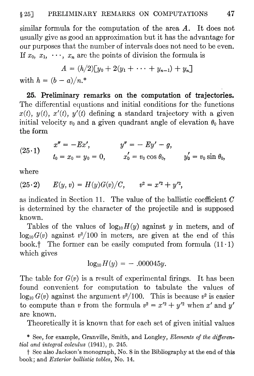
25. Preliminary remarks on the computation of trajectories 47
26. The method of computation of a trajectory . 49
27. Plans for the computation 52
28. The differential analyzer and its constituent parts . . 55
29. The differential analyzer for a simple illustrative equation 57
30. The differential analyzer for a trajectory 59
Chapter V
DIFFERENTIAL CORRECTIONS
31. Introduction 63
32. The differential equations of disturbed trajectories 63
33. Functions of lines in ballistics. . . 65
34. Adjoint systems of differential equations and a funda¬
mental formula ... 68
35. The adjoint equations and the fundamental formula for
trajectories ..... 68
36. Differential corrections for the range 71
37. Differential corrections for the г-coordinate of the point
of fall, in particular, for a cross wind . . 74
CONTENTS vii
38. Approximate solution of the adjoint system of equations 75
39. Gronwalhs method for integrating the adjoint equations 78
40. Weighting factor curves. Ballistic wind and density . . 81
41. Differential corrections for time of flight, maximum
ordinate, and angle of fall 85
42. Differential corrections for variations from normal in the
velocity of sound 87
43. Differential corrections to account for the sphericity of
the earth 89
44. Differential corrections to account for the rotation of the
earth 92
Chapter VI
BOMBING FROM AIRPLANES
45. Introduction . . 98
46. Bomb trajectories 98
47. Conditions for hitting when the flight is horizontal. 100
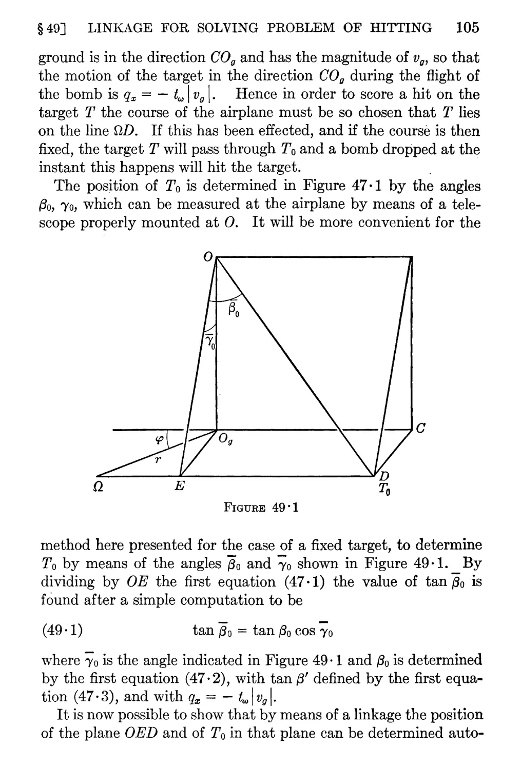
48. Determination of the ground speed vector .... 103
49. A linkage for solving mechanically the problem of hitting 104
TABLES FOR COMPUTATION
I. Values of logio G(v) tabulated against z;2/100 in meters 110
II. Values of logio Я(?/) tabulated against ?/in meters ... 117
III. Values of d log G(v)/v dv = G'/vG tabulated against
y2/100 in meters 120
IV. Coordinates, velocities, accelerations for a trajectory
having vz = 563 m/s, 0O = 21° 7', C = 2.512 .... 122
V. Solutions of the adjoint equations for range corrections
for the trajectory of Table JV 123
Bibliography 125
Index 127
CHAPTER I
THE NEED FOR MATHEMATICS IN EXTERIOR
BALLISTICS
1. Introduction. A battery commander in the field uses mathe¬
matics of a rather elementary sort for the determination of the rel¬
ative geographical positions of his battery and target, and for fire
control after these positions have been determined. For problems
in orientation he needs elementary surveying methods, and for fire
control he must be an expert in the use of range tables. For both
purposes he must have a thorough training which only skilled
military specialists can give.
Underlying the technique of the officer in the field, however,
there is mathematics for various auxiliary purposes of a consid¬
erably more serious nature. The construction of military maps,
for example, is a complicated problem of differential geometry,
fundamental for the orientation of a battery. A book of consid¬
erable size could be written on this subject alone. The present
pages, however, are devoted to the mathematics, mostly elemen¬
tary calculus and differential equation theory, which underlies the
construction of the range tables upon which the methods of fire
control are based, and without which these methods would be
seriously crippled and ineffective. In this first chapter some of
the problems of the battery commander are described quite
roughly, not for the specialist, but only so that the reader may see
the reasons why the mathematical developments of later pages are
justified.
2. The structure of ballistics as an applied mathematical science.
The subject of exterior ballistics is an excellent example of an ap¬
plied mathematical science.* Like every such science it consists
of three parts: first, a mass of experimental data which needs to be
systematized and correlated; second, a purely mathematical theory
* See Bliss, Mathematical interpretations of geometrical and physical phe¬
nomena, American Mathematical Monthly, XL (1933), 472-480.
1
2
MATHEMATICS IN EXTERIOR BALLISTICS £Сн. I
designed to fit the data and correlate them; and, third, there is the
necessity of checking the results of the theory with the data al¬
ready accumulated or with the results of new experiments, to see
whether or not theory and practice agree with the desired degree of
accuracy.
There is in general no strictly logical connection between the
observed data and the pure mathematical theory designed to cor¬
relate them, and no unique mathematical theory by means of
which the data can be coordinated. One must choose the basis of
the mathematical theory so that it corresponds to the given data
with the desired degree of accuracy, with the hope that the theory
may predict new results of importance. Similarly there is no rigid
reason why the results of the mathematical theory should agree
with the physical facts with the desired degree of accuracy, and to
be assured one must check by experiment in all important in¬
stances. The logical part of the theory is the structure of the purely
mathematical science designed to predict new results and to bring
some sort of order to those already observed. It is for the most
part the pure mathematical theory which is to be exhibited in the
succeeding pages of this book.
In the theory of exterior ballistics the differential equations set
up to describe trajectories have been always quite loosely co¬
ordinated with the observed facts, and they will doubtless be modi¬
fied and unproved from time to time in the future as they have
been in the past. The differential equations for the motion of a
projectile in a vacuum, for example, give as the trajectory a parab¬
ola which agrees also quite well with the actual path of a heavy
body projected at relatively low velocity through the air. The ef¬
fect of air resistance in that case is relatively small. The Siacci
theory in exterior ballistics, described in Chapter III, is effective
for the trajectories in air with low initial inclinations for which the
theory was designed, but when guns began to be fired at higher
inclinations new methods had to be developed. The differential
equations of this more recent theory will doubtless again give way
in the not distant future to equations which may more accurately
describe the effects of the rotation of a projectile.
The remarks in this section are made with the purpose of warn¬
ing the reader that he must not expect a unique theory of exterior
§3]
MILITARY MAPS
3
ballistics precisely related to experimental facts. The equations
now used in the theory have been tested, however, and found to
describe data observed in the field as accurately as one could hope
to have them at the present time.
3. Remarks on military maps. The problem of the military
map maker is to represent a portion of the surface of the earth upon
a plane in such a way that distances and directions on the earth’s
surface are preserved to scale on the map with accuracy sufficient
to be useful for fire control. It is well known to mathematicians
that the surface of a sphere cannot be mapped upon a plane so that
all distances are preserved to scale. This will be evident intui¬
tively if we think of trying to flatten a piece of a sphere upon
a plane. The spherical surface will always have to crack. But a
very small portion of a spherical surface will lie very close to a
plane tangent to it, and a correspondence between points on the
two surfaces can be specified in such a way that the distance be¬
tween every pair of points on the spherical fragment will be very
nearly equal to the distance between the corresponding points on
the plane. In this section two of the correspondences which turned
out to be useful for military maps in World War I will be briefly
described.
The first of these maps is called a Bonne projection and is based
upon a simple geometrical correspondence. Consider the sphere in
Figure 3 • 1 which is to be mapped upon the plane in Figure 3 • 2.
We draw sample parallel circles on the sphere and consider a cone
tangent to the sphere along one of them, say FOE. On the plane
in Figure 3-2 we draw a vertical line C'O' equal in length to CO,
and draw concentric circles with centers at Cr which will presently
be made to correspond to the parallel circles on the sphere. Each
point P on the sphere determines arc lengths OQ and QP. These
lengths measured off on the vertical line O'Q' and the circle Q'P',
respectively, determine uniquely a point Pr on the plane in Figure
3-2. For the map so constructed the parallel circles QP on the
sphere evidently correspond to concentric circles with centers at
the point O' on the map in Figure 3-2, and meridian circles NP
on the sphere correspond to arcs N'P' on the plane, all passing
through the point N' for which the distance O'N' is equal to the
length of the arc ON on the sphere.
4
MATHEMATICS IN EXTERIOR BALLISTICS £Сн. I
On the maps so constructed it is evident that distances between
corresponding points on the arc OQN and the straight line O'Q'N'
are equal, and corresponding dis¬
tances on parallel circles are also
preserved. It is provable that for
two curves on the sphere which
meet on the initial meridian circle OQ or on the initial parallel cir¬
cle OE the angle between them is the same as that between the
corresponding curves on the plane. But distances and angles on
the sphere other than those just described are distorted on the
map. If the point О is taken at a centrally located point of the
portion of the spherical surface which it is desired to map, then dis¬
tances and angles will be very nearly preserved on the map if the
neighborhood of О mapped is sufficiently small. A further property
of Bonne’s projection not so important for artillery fire is that the
areas of corresponding figures on the sphere and the map are equal.
Lambert’s projection is a second map which makes it possible to
map angles exactly and distances with close approximation over a
larger area than can be attained by the Bonne projection. We
again seek a representation which will map the parallel circles on
the sphere in Figure 3 • 3 into the concentric circles with centers at
C' in Figure 3-4. Each point P on the sphere has a latitude <p and
a со-latitude u = 7r/2 — <p, and a longitude v, as shown in Figure
3-3. Let R(u) be the radius of the circle QfPr of Figure 3-4 cor¬
responding to the arbitrary parallel circle with со-latitude и in
Figure 3 • 3. Let I be an arbitrarily chosen constant, and let Q'P'
§3]
MILITARY MAPS
5
be the arc indicated in Figure 3-4 which subtends the angle Iv at
C'. Then every point P on the sphere in Figure 3-3, with co¬
ordinates (u, v) as described, determines a unique point P' in
Figure 3*4
Figure 3 • 4 whose polar coordinates, with C" as center and C'O' as
initial line, are lv}.
It has been shown * that when the correspondence between
parallel circles on the sphere and the plane is specified by a function
of the form
R(u) = KEtan(u/2)J,
where К, I are arbitrary constants, the map will preserve angles.
It is not necessary to discuss the proof here. Such a map is said to
be conformal, the conformality of the map meaning that the angle
between every pair of intersecting curves on the sphere is equal to
the angle between the two corresponding curves on the plane at
their point of intersection. The arbitrary constants К and I can
furthermore be determined so that on each of two parallel circles,
say FDE and KGH, the length of every arc will be equal to that of
the corresponding arc on the plane. Thus on the Lambert map so
determined angles are preserved everywhere and distances are
preserved to scale, not on every parallel circle, as in the Bonne
projection, but on two arbitrarily selected parallel circles.
* See Adams, General theory of the Lambert conformal conic projection, Special
Publication No. 53, Department of Commerce, Washington, D.C., p. 23. The
argument there is for an ellipsoid of revolution.
6
MATHEMATICS IN EXTERIOR BALLISTICS [Сн. I
Suppose that a region of the earth’s surface is to be mapped on
a plane. We select a latitude </>0 midway between the extreme lati¬
tudes of the region, say that of the point 0 on the sphere, and we
select further two latitudes equidistant on each side of <p0 as the
latitudes of the parallel circles FDE and KGH on which distances
are to be preserved to scale. Then the map constructed as de¬
scribed above will be conformal and will have distances very nearly
accurate to scale over the whole zone bounded by the two parallel
circles and for some distance beyond them on each side, provided
that these parallel circles are taken sufficiently near to each other.
Thus on a map with = 49.5° and with KGH and FDE at lati¬
tudes 47.7° and 51.3°, respectively, it is found that errors in dis¬
tance on the map will not exceed .05 per cent in the zone between
the latitudes 46.8° and 52.2°.* For a range of 10 kilometers (about
6*4 miles), for example, this would imply a maximum error of 5
meters in the representation of distances on the map, which is well
within the probable error in the range of a projectile fired that dis¬
tance from a gun.
The description above has concerned the representation of a
sphere on the plane. The earth is an oblate spheroid and for such
a surface a Lambert projection is also possible.
4. Remarks on the orientation of a battery and the determina¬
tion of the map range and map azimuth of a trajectory. For use
in the field a military map has two mutually perpendicular systems
of parallel straight lines marked on it, one system approximately
east and west and the other approximately north and south.
These markings are called the grid of the map and are used as the
basis of a system of Cartesian coordinates. The origin of the co¬
ordinate system is taken at some point to the west and south of the
field covered by the map so that all points on the map will have
positive x- and ^/-coordinates. On a Lambert map the north and
south line O'C' in Figure 3 • 4 may be taken as one north and south
line of the grid of the coordinate system, and the other lines of the
grid are parallel and perpendicular to this initial one. The images
on the map of the meridian circles on the sphere are slightly in¬
clined to the north and south lines of the grid since these images
* See Adams, loc. tit.
§4] MAP RANGE AND AZIMUTH OF A TRAJECTORY .7
are straight lines passing through a common point C'. Images
on the map of parallel circles on the sphere are not coincident with
the east and west lines of the grid since on the map the images of
parallel circles on the sphere are themselves circles with centers at
Cf. At each point P' of the map, therefore, there are three north¬
ward directions, geographic north determined by the meridian
through Pf, grid north determined by the north and south grid
line through P', and magnetic north determined by the direction
of the needle of a compass at P'. The divergence between grid
north and geographic north at a point P' of the map is simply the
angle Iv in Figure 3-4, since the grid line through the point P' is
parallel to the line O'Cf of the map. Magnetic north is determined
by magnetic surveys and its divergence from geographic north is
indicated on the map. The angle measured clockwise from geo¬
graphic north at a point P' to another line through P' is called the
azimuth of the line at P'. The angle measured clockwise from grid
north to the line is called the gisement of the line at P'.
The field covered by a large scale military map is likely to be
about 10 kilometers square, and the grid lines are spaced 1 kilo¬
meter apart. Distances may be accurate to .05 of 1 per cent, as
indicated in a preceding paragraph of this section. Divergences of
magnetic north from geographic north are practically constant over
such a field and may be marked on the margin of the map once for
all. On the map are many reference points, church spires, hill tops,
prominent trees, etc., whose coordinates have been determined with
accuracy by surveys. These coordinates are indicated beside each
such point of the map in meters, though in measuring distances on
the map larger units may be used when less accuracy is needed.
When a battery takes a firing position in the field some of the
first duties of the orientation officer are (1) to determine the
direction of grid north from the position В of the battery, (2) to
determine the coordinates of B, and (3) to determine the altitude
of В in meters above sea level. Magnetic north may be determined
by means of a compass at B, or geographic north may be found
from an observation on Polaris or the sun or from other astro¬
nomical observations. When either of these is known grid north
is determined since the angle between grid and geographic north
is lv, and since the deviation of magnetic north from geographic
8
MATHEMATICS IN EXTERIOR BALLISTICS [Сн. I
north is marked on the map. When north has been determined
and a reference point corresponding to Q on the map is visible
from the battery the coordinates (xi, yi) of В can be determined,
since the gisement angle Vi and the distance d in Figure 4-1 can be
measured by means of surveying instruments, and coordinates of В
are then given by the formulas
Xi = x2 — d sin Vi, yi = y2 — d cos Vi.
The coordinates (x2, y2) of the refer¬
ence point Q are of course supposed
given on the map.
A contour line on the map is a line,
in general curved, all of whose points
are at the same altitude above sea
level. The altitude of each such line
in meters is indicated near the line
on the map. If the point В lies on
such a contour line its altitude is
known. If it lies between two such
lines its altitude can be determined with a fair degree of accuracy
by a simple interpolation. If greater accuracy is needed a survey
can be made to В from a reference point Q of the map whose alti¬
tude is known.
When the coordinates (яз, Уз) of a target T are known the
gisement v and range R of the line ВТ from the battery to the
target in Figure 4-1 can easily be calculated by the formulas
Я2 = (хз - Ж1)2 + (уз - У1)2, tan v= (хз- Xi)/(уз - yi).
If now a range table is at hand listing elevations against ranges
for the type of gun and projectile used by the battery, it might
seem that the problem of fire control is solved, since the gisement v
should specify the direction toward which the gun should be
aimed, and the range R should determine by means of a range
table the elevation of the gun necessary for the projectile to reach
the target T. This is, however, not the case. The map range
as calculated above must be corrected for a variety of disturbing
causes some of which will be described in the next section. One
of them which may be mentioned here is the difference in altitude
§5] DATA FOR CORRECTED RANGE AND AZIMUTH 9
between the gun В and the target T which is of course known
when the altitudes of В and T above sea level are known.
5. Sources of data for determining the corrected range and
azimuth. To determine just how a gun should be laid in order to
hit a target one must make use of a suitable range table. Some of
the data specifying the range table to be used for a particular gun
and also determining the corrections which must be applied to
the range and azimuth as read from the map are as follows:
(1) Name of gun, type of shell, fuze, powder charge.
(2) Data from the map.
Map range.
Map azimuth.
Height of target above gun.
(3) Materiel data.
Weight of projectile relative to normal.
Temperature of powder charge relative to normal.
Cant of axle of gun.
(4) Data from meteorological message.
Altitude above sea level at meteorological station.
Air temperature at station.
Ballistic wind.
Ballistic density of air.
For each type of gun, shell, fuze, and powder charge a separate
range table must be provided. The data under (1) determine
which one of these tables must be used.
In the preceding sections a description of the determination of
the data in (2) from the map has been given.
The first two titles under (3) indicate causes which change the
initial velocity of the projectile from normal. Each projectile is
marked with one of the markings
■ ■ ■■, ■ ■■■, ■ ■■■■> ■■■■■■-
The weight is normal when there are four squares, and greater or
less than normal when the number is greater or less than four.
The temperature of the powder charge relative to normal (70°F)
is inferred from the temperature of the dug-out or other storage
place where the charges are stored. The final item under (3) is
the cant of the axle of the gun due to unevenness in the ground.
10
MATHEMATICS IN EXTERIOR BALLISTICS [Сн. I
If the axle is not horizontal the vertical plane through the axis of
the gun after elevation will be different from the vertical plane
through the axis before elevation and a correction to the azimuth
setting must be made.
The flight of a projectile is affected by air temperature and
density, and of course by the wind. The meteorological message
furnishes the data in this connection. To determine the wind a
balloon a few feet in diameter is sent up and its position is de¬
termined from time to time by observing it with surveying instru¬
ments. The rate of rise of the balloon being known, this process
will give a sequence of vectors representing the velocities of the
wind at various altitudes. To determine the densities of the air
at various altitudes an airplane or some other device can be sent
up to record the temperatures and pressures of the air. From
these the densities can be calculated by a simple formula.
A single meteorological station will furnish data for many bat¬
teries by means of messages which are sent out several times a
day by radio in very condensed form. Such a message gives the
altitude of the station in feet above sea level, the temperature of
the air at the station in Fahrenheit degrees, and the so-called
ballistic wind and density for several different altitude intervals.
By an altitude interval is meant an interval from 0 to a certain
number h of meters. By ballistic wind for a certain altitude interval
is meant a wind constant in direction and velocity at all altitudes
which would have the same effect on a projectile flying in that
interval as the observed winds. The latter may of course have
quite different directions and velocities at different altitudes. By
ballistic air density for a certain altitude interval is meant a cer¬
tain percentage of normal air density, the same at all altitudes,
such that for a projectile flying in that interval the effect of the
constant variation from normal of the hypothetical constant bal¬
listic air density would be the same as that of the observed densi¬
ties. The percentage variation from normal in the observed den¬
sities will in general not be constant but will vary from altitude
to altitude. It is the duty of the staff of a meteorological station
to determine the ballistic winds and densities for various altitude
intervals from the observed winds and densities. More will be
said about this in Section 39. In order to correct for wind and air
THE USE OF THE RANGE TABLE
11
§ 6 J
density the fire control officer must know approximately the
maximum ordinate yQ of his proposed trajectory, so that he can
determine the altitude interval in which the trajectory will lie.
The altitude interval of the meteorological message from which
he must take ballistic wind and density will then be the one for
which the maximum ordinate h of the interval is the nearest one
exceeding the maximum ordinate go of the trajectory.
The above list of data to be applied in the laying of a gun is
not complete. For very long range guns, for example, corrections
may be needed to account for the effects of the rotation or spheric¬
ity of the earth, and there are other corrections which may be
necessary which have not been mentioned here.
6. The use of the range table. The characteristics of a tra¬
jectory which must be taken into account in firing a gun, in par¬
ticular the corrections necessary for map range and map azimuth,
are taken from a range table corresponding to the type of gun,
shell, fuze, and powder charge which are to be used, as indicated
above. The principal column of the range table is a list of ranges
extending from zero to the maximum possible range for that par¬
ticular gun and projectile, the entries being usually 100 yards
apart. In a second column, opposite each of these ranges, is the
elevation which will give that range for a standard trajectory at
sea level undisturbed by wind, abnormal density, or other causes.
Each of the correspondences, range to elevation, belongs to a
separate trajectory. One of the principal problems of range
table construction is the computation of standard trajectories cor¬
responding to initial elevations sufficiently close together so that
the remaining range elevation correspondences can be determined
by interpolation.
Not all of the data in the range table can be described here.
Only enough will be mentioned so that the reader can see clearly
the need for mathematics in the construction of the table. In the
table are columns for the maximum ordinate, terminal velocity,
angle of fall, and time of flight of each trajectory, all of which are
found from the computation of the trajectory. The maximum
ordinate is used in determining the altitude interval of the tra¬
jectory, so that corrections for ballistic wind and density can be
properly calculated. The terminal velocity and angle of fall are
12
MATHEMATICS IN EXTERIOR BALLISTICS [Сн. I
useful in estimating the destructive power of a hit by a shell.
The time of flight is needed for timing a fuze of a shrapnel shell,
for example, so that the shell will explode at the proper point on
the trajectory.
The range of a trajectory is the distance OR from the initial
point О of the trajectory to what would be the point of fall R of
the projectile on the horizontal plane through 0, as shown in
Figure 6-1. If the target T is not in the horizontal plane OR the
range read from the map will be OQ, and this must evidently be
increased for a trajectory passing through T when T is above the
horizontal OQ as in the figure, and decreased when T is below OQ.
The range table gives for different ranges OQ the increases or de¬
creases QR corresponding to various altitudes QT of the target T
above or below Q.
The map range must also be corrected for variations in initial
velocity due to various causes, and the range table gives for each
range the corrections corresponding to changes in initial velocity.
The changes in velocity to be accounted for are due to variations
from normal in the weight of the projectile and the temperature
of the powder charge, and sometimes to other causes.
Variations from normal conditions in the air cause variations in
the range of a projectile. Thus a variation in temperature from
standard (59°F or 15°C) will affect the elasticity of the air. The
projectile will fly farther in air of higher temperature. A follow¬
ing or opposing wind will of course affect the range, and air density
lower than normal will increase the range. The fire control officer
knows his altitude above sea level, and therefore also his altitude
above his meteorological station, since the altitude of the station
is given in the meteorological message. He has the air temoera-
ture and ballistic density at the station from the message, and can
therefore easily compute the temperature and ballistic density at
his own gun, since the laws of variation of air temperature and air
THE USE OF THE RANGE TABLE
13
§63
density with altitude are well known. Knowing the variations
from normal in the air temperature and ballistic density at the
battery he can find the corresponding corrections to the range in
the range table.
Corrections which must be applied to map azimuth are due to
cross wind, cant of axle, and drift. Like the corrections to range
they are listed in the table. The drift is due to the rotation of the
projectile.
The purpose of the remarks in the preceding paragraphs is to
show the importance of the range table for the control of the fire
of a battery in the field. The corrections to map range and azimuth
doubtless seem numerous and complicated. But an artillery
officer in the field is a highly trained specialist. His computations
are made on forms which have been carefully planned and tested.
After the firing data have been accumulated the calculation of the
corrections to map range and map azimuth with the help of a
range table is a matter of a few minutes.
The business of the mathematical ballistician is to compute the
data required for range tables and to assist in the arrangement of
the data in a form as convenient as possible for use in the field.
The purpose of this book is the exposition of some of the mathe¬
matics which is used in that connection. The methods applied in
computing trajectories from their differential equations and in
finding the differential corrections to a trajectory due to disturb¬
ing influences of various sorts are mathematically interesting in
themselves and can be of service in other fields as well as ballistics.
Some of these methods are described in the following chapters of
this book.
CHAPTER II
THE DIFFERENTIAL EQUATIONS FOR A
TRAJECTORY
7. Introduction. The problem of determining the motion of a
spinning projectile shot through the air from a rifled gun is mathe¬
matically a very difficult one which has not so far been completely
solved. The forces acting upon the projectile as a result of its
motion through the air are not as yet completely known. Attempts
have been made to describe the motion of the projectile on the
assumption that the forces acting, besides the force of gravity,
are a so-called drag in the direction on the tangent to the trajectory
opposite to the motion of the projectile, and a cross wind force
at right angles to the drag due to the deviation or yaw of the axis
of the projectile from the tangent. But the effect of the rotation
of the projectile is in any event difficult to account for. Fortu¬
nately there are some simpler special cases of projectile motion
which can be handled mathematically and which have proved to
be of value in practice though they do not correspond precisely
to the physical situation. The simplest of all is the theory of
motion of a projectile in a vacuum. It has considerable value as
a means of introducing notations which are commonly used in
ballistic theory, but the parabolic trajectories found are quite
inaccurate for describing the motion of projectiles in air. When
the velocity is low and the projectile heavy, so that air resistance
is very small compared with the pull of gravity, the parabolic
trajectories of motion in a vacuum give a very fair picture of what
actually happens. Such motion will be discussed briefly in the
next section. A second special case which has been found most
useful is the one in which the rotation of the projectile is ignored
and the only forces acting on the projectile are assumed to be the
drag and gravity. The part of this chapter following Section 8 on
parabolic trajectories is devoted to setting up the differential
14
§8]
TRAJECTORIES IN A VACUUM
15
equations of motion which are the basis of this important theory.
8. Trajectories in a vacuum and notations. In the following
pages primes will be used to denote derivatives with respect to
the time t. Thus x' and x" will denote the first and second deriva¬
tives of x with respect to the time, and similarly for other variables.
The rry-coordinate system used to describe a trajectory will always
lie in a vertical plane and have
its origin at the initial point of
the trajectory, as shown in Fig¬
ure 8-1. For motion in a vacuum
the only force acting upon the
projectile P is the force of gravity
directed vertically downward. It
Figure 8*1
is equal in magnitude to mg, where m is the mass of the projectile
and g is the acceleration due to gravity. The equations of motion,
mx" = 0, my" = — mg,
arc found as usual by equating the components (mx", my") of
the inertial force to the components (0, — mg) of the force of grav¬
ity impressed upon the projectile.
Unless otherwise expressly stated we use the subscript 0 to
designate values of variables at the origin of the trajectory. The
differential equations of motion and the initial conditions can
then be written in the form
(8 • 1) X r f
Xo = yo = 0, Xq = Vq cos 0o, yQ = Vo sin 0O,
where v is the velocity and 0 the inclination of the tangent to the
trajectory at the projectile, and the time at the origin is t — 0.
The differential equations and initial conditions (8-1) completely
determine the trajectory. Their solutions are found by well-
known elementary methods of the calculus to be
(8-2) x = tv0 cos Oo, у = tvo sin 0o — gt2/2.
By eliminating t we find that the curve of the trajectory is given
by the equation
(8*3) у = x tan 0o — gx2/2vo2 cos2 0O.
This shows that the trajectory of a projectile in a vacuum is a
16 DIFFERENTIAL EQUATIONS FOR A TRAJECTORY [Сн. II
parabola with its axis vertically downward. The equations (8-2)
give the position of the projectile on the parabola at each time L
We may as well begin to familiarize ourselves with some of the
notations in current use in ballistic theory, as indicated in Figure
8-1 and in the following list:
vQ - initial velocity
= quadrant angle of de¬
parture
= initial inclination of the
tangent to the tra¬
jectory
Q = point of fall
a: = angle of fall
хш = range
= time of flight
v„ = velocity at the point of fall
(zs, y5) = coordinates of summit
These quantities can all be easily calculated for the parabolic
trajectory (8-2). The range is the coordinate of the point on
the trajectory where у = 0. From equations (8-2) we find then
that the time of flight and range are
(8-4) = (2y0 sin 0o)/y, хш = (v20 sin 26o)/g.
From the equations
tan co = — dy/dx = — y''/x', v2 = x'2 + y'2
evaluated at t = we find the angle and velocity of fall to be
(8-5) w = 0O, v» = v0.
Finally, at the summit of the trajectory where the derivative
dy/dt = Vo sin 0o — gt
vanishes, we find
(8-6) ts = 'V" S‘n ''s = sin 20°)/2Л
У, = (i»o sin2 0o)/2<7 = gC/8.
From the first equation (8 • 2) it is evident that the velocity xf in
the x direction is always the constant Vo cos 0O.
The equations (8 • 2) enable us to answer a number of questions
about trajectories in a vacuum. Let Vo be fixed. The maximum
possible range хш for different values of 0O is then found by setting
equal to zero the derivative with respect to 0O of the second ex¬
pression (8-4), solving for 0o, and substituting the solution in the
§9]
EQUATIONS FOR TRAJECTORIES IN AIR
17
second expression (8-4). The maximum range so calculated is
corresponding to the quadrant angle of elevation % = я/4.
Eor each range хш < Vo/g, the second equation (8-4) has two solu¬
tions of the forms dQ = 7r/4 ± <p, symmetric with respect to тг/4.
It follows that for a given initial velocity each range less than the
maximum one possible can be at¬
tained with two different quadrant
angles of elevation, as indicated
in Figure 8-2. The trajectories
with fixed v0 and variable d0, as
assumed above, have an envelope
found by setting equal to zero
the derivative of the expression
(8-3) with respect to do, solving
for do, and substituting the solu¬
tion in equation (8-3). The envelope thus found is the parabola
у = Vo/2g - gx2/2v20
shown in Figure 8-2.
9. The differential equations for trajectories in air. Consider
a projectile with mass m starting from the origin in a vertical
rr?/-plane, having initial velocity v0 as indicated in Figure 9-1, and
acted on only by the force of gravity mg and the drag D of the air
in the backward direction along the tangent. The differential
Figure 9 • 1
equations of motion and initial conditions at t = 0 then have the
form
(9-1) mx" = ~ D cos тУ" = ~ D sin d — mg,
Xo = у о = 0, Xo = Vo cos do, Уо = Vo sin d0,
where d is the inclination of the tangent defined by the equations
(9-2) cos d = x'/v, sin d = yf/v, v2 = x'2 + y'2.
18 DIFFERENTIAL EQUATIONS FOR A TRAJECTORY [Сн. II
For a projectile symmetric about an axis and moving with its
axis always in the tangent to the trajectory, the equations (9-1)
would be accurately descriptive. These conditions are, however,
never attained in practice. A projectile shot from a rifled gun
does not have its axis of symmetry always in the tangent to the
trajectory, but because of its spin its axis precesses. 'The preces¬
sion is clockwise about the tangent, to an observer facing forward,
Figure 9*2
when the spin is clockwise. If the projectile is well designed its
axis turns so as to stay approximately in the direction of the
tangent to the trajectory throughout the flight. The components
of air resistance in directions other than tangent to the trajectory,
owing to the so-called yaw between the axis of the projectile and
the tangent to the trajectory, cause a drift to the right which can
be taken into account experimentally but which is difficult to
predict theoretically. The equations (9-1), with properly chosen
drag functions D, have been found to give valuable first approxi¬
mations to the flights of projectiles. They need modifications to
account for various disturbances due to wind, abnormal density
of the air, and other causes, as we shall see in Chapter V.
So far the variables upon which the drag D is dependent and
the form of the dependence have not been specified. In the next
section is given a determination of the form of the drag function D
which is based upon dimension theory and an assumption con¬
cerning laws of physics. It gives a justification for the form used
for D in ballistic theory which might otherwise seem rather arti¬
ficial. The form so determined has been amply justified in prac¬
tice. The argument in Section 10 is theoretical in character.
It may be omitted by the reader who is willing to accept the equa¬
tions of a standard trajectory in the form suggested by the more
intuitive argument given in Section 11 and justified by experience.
10. The form of the drag function. Let us consider here a
class of projectiles all of which have the same shape, though their
THE FORM OF THE DRAG FUNCTION
19
§ 102
sizes and weights may be different, and let us consider further
only flights of such projectiles in the direction of their axes. The
drag of the air on one of these projectiles for such a flight is as¬
sumed to be a function D (p, d, v, a) of the density p of the air,
of the diameter d and velocity v of the projectile, and of the ve¬
locity of sound a. That D should depend upon the three varia¬
bles p, d, v is easily understood. When these are fixed the drag
still varies with a, or, what is the same thing, with the tempera¬
ture of the air, since the velocity of sound in air has been experi¬
mentally related to the temperature of the air by the formula
(10-1) а = а8(Т/Т^.
Here T is the absolute temperature, Ts is the so-called standard
value of the absolute temperature (518.6 in Fahrenheit degrees,
corresponding to 59°F or 15°C), and as is the velocity of sound at
this standard temperature. The assumption that D depends
upon a is justified by experience and is also natural since the drag
of the projectile is largely due to its loss of energy in the forma¬
tion of waves in the air, and these waves are quite different and
cause different retardations for velocities of the projectile above
and below the velocity of sound.
The laws of motion for a projectile should be the same what¬
ever units of length, mass, and time are used. If the values of the
quantities x, y, m, p, d, v, a, g, expressed in terms of new units,
are designated by the subscript unity the new equations of motion
should have the same form as (9-1),
(10-2) miX" = ~ D(p1’ d1’ V1) ai^x^V1’
m^yi = - D(P1, di, vi, a^yi/vr -
with the same drag function. If the ratios of the old to the new
units of length, mass, and time are the constants L, M, T the
equations (10-2) are equivalent to
(ML/T^mx’' = - D[(M/L3)p, Ld,(L/T)y,(L/T)a>'/v
and a similar second one for т/. If the last equation is equivalent
to the first one in (9-1) we must have
(10-3) D[(M/L3)p, Ld,(L/T)v, (L/T)a] = (ML/T2)D(p, d, v, a)
and this equation must hold for all positive values of L, M, T.
20 DIFFERENTIAL EQUATIONS FOR A TRAJECTORY [Сн. II
If we introduce the values
L = 1Д M = L3/p = 1/pd3, T = vL = v/d,
equation (10-3) becomes
Z>(1, 1,1, a/v) = (1/p d2v2)D(p, d, v, a)
which shows that D must have the form
(10-4) Z)(p, d, v, a) = pd2v2 KD(v/a).
In this formula the coefficient KD is independent of the units used,
since it depends only upon the ratio v/a. It is called the drag
coefficients
The differential equations of motion in (9-1) are now easily
seen to have the form
(10-5) x'f = —Exf, y" = -Ey'-g
if we use the notations
(Ю-6) E = [>(?/)/Po]GO, a, Po)/G
where
(10-7) G(v, a, p) = pvKD(y/a), C = m/d2.
The symbol p(y) stands for the density of the air at the altitude y,
and po is the density at the level у = 0 of the origin of the trajec¬
tory. The constant C = m/d2 is called the ballistic coefficient.
The function G usually tabulated from experiment is the special
function
(10-8) G(v) = G(v, a„ p3) = p.vK^v/a,'),
where ps is the standard density of the air at sea level. The values
of G(v, a, p) can be found from a table for G(v) since from (10-8)
KD(v/a) = KDias(v/a)/as2 = il/psas(v/a)JG(aav/a),
and since it then follcrws from (10-7) that
G(v,a,p) = (p/p,')(a/a,)G(a,v/a).
With (10*1) and the next to last equation this gives
(10-9) G(v, a, P) = (р/р.)(Т/ТаГв[у(Т,/т
The values of G(v) are in practice tabulated against the values of
* See Hayes, Elements of ordnance, p. 412; Exterior ballistics, p. 16.
§11]
EQUATIONS OF A STANDARD TRAJECTORY
21
?j2/100 instead of v since v2 is easier to compute than v from the
formula in (9-2) when xf and yr are given. The table for G(v)
can be adjusted to the units used in measuring m and d by the
introduction of a constant factor. In this book the units used
are always supposed to belong to the metric system unless other¬
wise indicated.
The argument of the preceding paragraphs is for a class of pro¬
jectiles having the same shape, and the value of the ballistic co¬
efficient has been defined to be C = ш/d2. For a long time it was
assumed that the same function G(v) would be effective for all
projectiles, and that the equations (10-5), (10-6), (10-7) could
be adjusted to describe the flight of an arbitrarily chosen pro¬
jectile by changing the value of C to C = m/id2 with a suitably
chosen value of i. The factor i is appropriately called the form
factor. More recently it has been found that projectiles fall into
classes each of which has its own special function G to be used
with ballistic coefficients of the form C = m/id2. Fortunately the
same function G can sometimes be used in this way for a class
of projectiles which do not all have exactly the same shape.
11. Normal air density and the equations of a standard tra¬
jectory. The ratio of the normal air density p(y) at the altitude у
above sea level to the standard density ps at sea level has been
determined from the average of many observations. The value
of this ratio usually accepted for ballistics is
(П-1) H(y) = 10~-000045// = е~,0001036у
when the altitude у is given in meters. Normal air densities at
all altitudes rarely or probably never occur simultaneously in
nature. But a trajectory can be computed for normal densities
and then corrected to account for the variations from normal
densities at different altitudes at the time of fire. Moulton *
gives theoretical reasons why the normal air density might well
be expected to be expressed by an exponential. One should note
that H(y) is also the ratio of normal air densities at any two alti¬
tudes у meters apart since two such densities have values of the
form psH(yi + y) and psH(yf) and since
Я(?У1 + у) = Н(У1)Н(у).
* New methods in exterior ballistics (1933), p. 49.
22 DIFFERENTIAL EQUATIONS FOR A TRAJECTORY [Сн. II
A standard trajectory may be defined mathematically as one
which is determined by differential equations and initial condi¬
tions of the form
(11-2) X" = ~ Ex'’ = ~Ey' “ g’
x(0) = ?/(0) = 0, z'(0) = v0 cos 0o, y'(0) = Vo sin
where
(11-3) E(y, v) = H(ffi)G(y)/C, C = m/id2.
In these expressions H(y) is the normal ratio (1Г-1) of the air
density p(y) at altitude у above the origin of the trajectory to the
density po at the level of the origin; G(v) is a so-called drag function *
like that defined in Section 10, to be determined by experimental
firings; and C is the ballistic coefficient which is also to be deter¬
mined experimentally for each projectile. The mass of the pro¬
jectile is m, the diameter of the maximum cross section of the
projectile perpendicular to its axis of symmetry is d, and i is the
part of C which is supposed to be adjusted to make the formulas
fit different projectiles. It is called the form factor.
In order to justify the formulas (11-2) and (11-3) for a tra¬
jectory we start again from equations (9-1). The drag D of the
air on a projectile moving in the direction of its axis should evi¬
dently be independent of the mass of the projectile but dependent
upon the density p of the air, the velocity v of the projectile, and
the area A = ird2/^ of the maximum cross section of the projectile.
Since D must vanish with each of these variables we may assume
quite arbitrarily that D is equal to the product of these variables by
a function Z>i(v) of v alone. Then
D = pvADr(v) = vH(y)G(v)d2
where G equals p07rDi/4, p0 is the normal air density at the origin
of the trajectory, and provided that the ratio р(у)/рь is the normal
density ratio (11-1). With this value of D equations (9T) take
the form (11-2) with E defined as in (11-3).
The formulas just found are based upon the assumption that
the drag D is equal to the product of the variables p, v, A by a
function of the velocity alone, an assumption which is justified
* The notation G (v) was suggested by the name of the French Gavre Com¬
mission which constructed a table for one of the early drag functions.
23
§12] DETERMINATION OF THE DRAG FUNCTION
only by its success. The argument of the preceding paragraphs of
this section is given only to show how the form (11-2) (11-3) of
the equations of a standard trajectory may have been suggested
in practice. The justification of equations (10-5), (10-6), (10-7)
in Section 10 seems more satisfactory than the one given in this
section for equations (11-2) and (11-3).
The equations (10-5) and (10-6) reduce to equations of a stand¬
ard trajectory with the forms indicated in (11-2) and (11-3) when
the density ratio p(y)/pv is everywhere equal to the normal ratio
H(y), when furthermore the origin is at sea level so that p0 = p3,
and when finally the temperature is standard so that a = as and
T = Ts everywhere. On the other hand equations (11-2) and
(11-3) with Я(г/) replaced by p(y)/p^ and G(v) by G(v, a, p0) from
(10-9), will be equivalent to (10-5) and (10-6). In Section 32 an
abnormal density ratio is accounted for in an equivalent way by
multiplying H(y) in (11-3) by a factor 1 + к(у) where
H(?/) [1 + к(у)] = p(y)/po.
In Section 42 a variation of the absolute temperature T from the
normal absolute temperature Ts is accounted for by replacing
G(v) in (11-3) by the function G(v, a, p0) from (10-9) with
T/Ts = 1 + r(y\
and with p0 = ps corresponding to the assumption there made that
the origin of the trajectory is at sea level.
12. Experimental determination of the drag function. For a
particular projectile shape regarded as standard the function G(v)
in (11-3) can be determined experimentally by means of horizon¬
tal firings at sea level.* If a projectile with the standard shape
has mass m and diameter d its ballistic coefficient may be defined
as the quantity C = m/d2, as was indicated in Section 11, and
then the function G(v) for that projectile shape can be determined.
The horizontal motion of the projectile is described by the first
of the equations (9-1) which is equivalent to the first of equations
(11-2). Since H(y) = 1 at sea level, С = and x' = v for a
horizontal firing, this equation can be written in the form
(12-1) x" = — vG(v) ddjm
* See Alger, Exterior ballistics (1906), p. 21.
24 DIFFERENTIAL EQUATIONS FOR A TRAJECTORY [Сн. II
with the help of the relations (11-3). Suppose now that the pro¬
jectile is fired through screens with abscissas Xi, x'lf x2, x2 as in
Figure 12-1, and that the times of passage through the screens
have been noted by a suitable timing device. The average veloci¬
ties Vi and v2 on the intervals xiXi and x2x2 are then determined and
x
X1 X1 X2
Figure 12 T
they may be regarded as the velocities at the mid-points of the
two intervals where t = h and t = t2. If we multiply the equation
(12*1) by x' and integrate from ti to t2 with respect to t we find
(12-2) (v2 — t?i)/2 = — (d2/m) I vG(v)x' dt = — {d2/m)G(v)x
if we regard the drag D = vG(v) as constant on the interval x
indicated in the figure. The value of the drag from equation (12 • 2)
is taken as its value at the mean velocity v = (t?i + v^/2.
Theoretically the function G(v), whose determination has just
been described, is effective for use in equations (11-2) and (11-3)
only for projectiles of standard shape. But it is found that these
equations with the same function G(y) may be made to describe
the flight of other projectiles also, whose shapes do not differ too
much from the standard one, provided that the ballistic coeffi¬
cients are taken in the form C = m/id2 with suitable constant
values for the form factors i. In earlier years it was assumed that
equations (11-2) and (11-3) with the same drag function could
be made to apply to every projectile in this way. But more
recently greater accuracy has been attained by distinguishing a
limited number of classes of projectile shapes each of which has a
separate drag function.
Methods for determining the velocities and drag functions of
projectiles have undergone long evolution.* Among the devices
* Alger, loc. cit., pp. 17 ff.; Bennett, Physical bases of ballistic table computa¬
tion, Ordnance Text Book, p. 4, War Department Document No. 92 (1920).
§12J
DETERMINATION OF THE DRAG FUNCTION
25
used have been the ballistic pendulum, the gun pendulum, the
Boulenge chronograph, and quite recent devices invented by in¬
vestigators at Aberdeen Proving Ground using firings through elec¬
trical fields. The most quoted tables of the drag function are those
of Mayevski (1883), and of the Gavre Commission (1888). The
latter table has been smoothed by fitting an analytic function to
it * and the table thus constructed has been the one most used in
computing trajectories by methods of approximate integration.
The later tables for different types of
projectiles have been prepared at Aber¬
deen Proving Ground.
It may be of interest as a matter of
curiosity to see how the velocity of a
bullet can be determined by means of
a simple pendulum. In Figure 12-2 let
OP be a pendulum with P at the center
of gravity of the bob of the pendulum
which is supposed to be a block of
wood. A bullet with mass and hori¬
zontal coordinate Xi strikes the bob and
imbeds itself in it. If the mass of the
bob is m2 and the horizontal coordinate
of its center of gravity is then dur¬
ing the imbedding of the bullet the accelerations and velocities
of the bullet and bob are related by the equations
(12-3) т^х" = — m2X2, тгх{ + т2х2 = с.
If v is the original velocity of the bullet at the moment of impact,
and V is the common velocity of the bullet and block after the im¬
bedding is complete then
(12-4) m^v = C = (mi + m2)V.
This is a consequence of the second equation (1.2-3) evaluated with
velocities v and 0 for the bullet and bob at the moment of impact,
and with the simultaneous velocities V for bullet and bob at the
moment when the imbedding is complete. The motion of the pen¬
dulum can be supposed to begin at the time t = 0 with the velocity
* Bennett, loc. cit., p. 4.
26 DIFFERENTIAL EQUATIONS FOR A TRAJECTORY £Сн. II
V, since the motion and time during the imbedding of the bullet
are very small. From the differential equation of the pendulum,
(mi + m2')a0" = — (mi + m2)g sin 0,
it follows by a simple integration and subsequent evaluation of the
constant of integration at t = 0 that
a20'2 = V2 — 2^a(l — cos O').
Hence at the top of the pendulum swing where 0' = 0, 0 = 30
we have
V2 = 20a(l — cos 9q) = 2gh,
where h is the altitude of the swing shown in Figure 12-2. Thus
from equation (12-4) the velocity of the bullet at impact is found
to be
v = (mi + m2)V/?ni = (mi + m2) (2gh^/ m^
an expression whose value is determined by the altitude h of the
swing caused by the impact of the bullet.
CHAPTER III
THE SIACCI THEORY
13. Introduction. The so-called Siacci method in exterior
ballistics * is the one which was commonly in use before the war of
1914-1918. It has in it an approximation which makes it possible
to integrate the differential equations of a trajectory by means of
quadratures, but which limits the application of the theory to
trajectories with relatively small quadrant angles of departure.
The scope of the theory was sufficient before World War I since it
was during that war that the use of trajectories with higher initial
elevations first became common. In view of modern artillery prac¬
tice the restriction to low elevations is a serious defect. But quite
recently it has been recognized by Hitchcock and Kent that the
Siacci theory with modified approximations may still have value
for trajectories with high initial elevations on which the variations
of the inclination of the tangent are small and the density of the air
approximately constant. In the exposition of the following pages
the notations are as nearly as pos¬
sible those of Hitchcock and Kent.
14. The differential equations
with the pseudo-velocity as inde¬
pendent variable. For the Siacci
theory variables u, t, x, y, 0 are
used instead of the variables t, x, y,
xf, y’ in equation (9-1), where tan 0
= yf/x' and и is the so-called pseudo¬
velocity defined by the equation
(14-1) и = x’ sec 0O = v cos 0 sec Oq
* References for this chapter are Alger, Exterior ballistics; Tschappat, Ord¬
nance and gunnery, Chapter IV; Hitchcock ancl Kent, Applications of Siacci1 s
methods to flat trajectories, Ballistics Laboratory Report No. 114 (1938), Aber¬
deen Proving Ground; Ingalls1 ballistic tables, Artillery Circular M.
27
28
THE SIACCI THEORY
[Ch. Ill
with 0Q the initial value of the inclination 6 of the tangent. The
variable и evidently decreases constantly on the trajectory, since
x' has this property. In terms of the new variables the differential
equations and initial conditions are easily found from equations
(11-2), (11-3), and the relation H/y) = p(y)/pn to be
dt/du = — р^С/puG(y),
dx/du = —poC cos 0Q/pG(v),
(14-2) dy/du = —pQC cos 0o tan 0/pG(v),
cZ(tan 0)/du = pQCg/[_pu2 cos OoG(v)J,
и = v0, t = x = у = 0, tan 0 = tan 0Q,
where p0 is the density of the air at the origin of the trajectory.
15. The Mayevski drag function and the Siacci approximation.
In the Siacci theory the drag function used is that of Mayevski
mentioned above in Section 12. The drag function at sea level in
Mayevski’s table is assumed to have the form D = vG(v) = kvn, in
which к and n are positive constants having different values for
different velocity zones, but chosen so that they define a continu¬
ous function over the whole range of velocity values to be con¬
sidered. The Mayevski table of zones and values of к and n is as
follows *:
Mayevski’s Table for the Drag Function
D = vG(v) = kvn
Zone for v in
foot-seconds
n
Log к
0- 790
2
5.66989 - 10
790- 970
3
2.77344 - 10
970-1230
5
6.80187 - 20
1230-1370
3
2.98090 - 10
1370-1800
2
6.11926- 10
1800-2600
1.7
7.09620 - 10
2600-3600
1.55
7.60905 - 10
These values for the drag function were found to be accurate
enough to be useful in the Siacci theory and have been used for a
long time for the purposes of exterior ballistics.
Since G(v) = kvn~r the value of this function in terms of the vari¬
able и in (14-1) may be expressed in the form
(15-1) G(y) = G(u) cos 0o(cosn~2 0o/cosn_1 0).
* Alger, loc. cit., p. 19; Tschappat, loc. dt., p. 430.
§15]
THE SIACCI APPROXIMATION
29
For a trajectory of low elevation the factor in parentheses is ap¬
proximately unity and the air density p(y) is everywhere very near
to the initial density p0 at the origin of the trajectory. If we make
use of these approximations the last equation becomes
(15-2) G(v) = G(u) cos в0
and the differential equations and initial conditions in (14-2) take
the form
dt/du = — C sec 3o/uG(u),
dx/du = — C/G(u),
(15-3) dy/du= — Ctan 0/G(u),
d(tan 6)/du = Cg/v? cos2 0O (?(u),
и = Vo, t = x = у = 0, tan в = tan 3Q.
These are the differential equations of motion after the approxi¬
mations H(y) = p/po= 1, cosn~2 0o/cosn‘_1 0 =1 of the Siacci
theory have been introduced. The normal air density varies but
little on a trajectory with initial elevation not more than 10°, so
the approximation H(y) = 1 is a good one. Some idea of the ac¬
curacy of the second approximation can be inferred from the fol-
lowing tables:
t
0
incr
ts incr
I' incr
0
e.
deer
0 deer
— 6q deer
COSn~2e0/COSn_10
sec0o
deer
cosn_20o incr
sec0o incr
COSn_20O/ СО8П_10Ш
The inclination в decreases from 0O to Зш on the trajectory. At the
summit it has the value 0 and at a time t' between ts and it will
have the value — 0O. On the larger part of the trajectory for
0 t t! the value of the fraction cosn~2 0o/cosn“1 в varies between
sec 0O and cosn_2 0O. For the initial elevations 0O = 5° and 0O = 10°
we have the following values for this maximum and this minimum:
00 =
-o
0o = 10°
n
sec 0o
cosn_20o
sec 0o
COSn 20O
2
1.004
1.000
1.015
1.000
3
1.004
.996
1.015
.985
5
1.004
.989
1.015
.955
1.7
1.004
1.001
1.015
1.005
1.55
1.004
1.002
1.015
1.007
These tables show that except on the relatively short part of the
30
THE SIACCI THEORY
[Ch. Ill
trajectory where t varies from tr to the value of the fraction
cosn_2 #0/cosn_1 в is near to unity.
The approximations which have been discussed above are not
necessary in the theory of Chapter IV and the following ones.
They would in part be unjustifiable for complete trajectories with
high initial elevations. But here again they may be useful for parts
of such trajectories which are relatively straight, as indicated in
Sections 19 and 20.
16. The integration of the approximate equations.* We now
introduce four so-called space, time, inclination, and altitude
functions. They are functions completely defined by the proper¬
ties that they are continuous and have the following derivatives
and initial values:
(16’1)
S'(u) = - 1/G(u\
T(u) = - l/uG(u),
I'(u) = - 2g/u2G(u\
A'(u) = - I(u)/G(u),
5(3600) = 0,
T(3600) = 0,
Л-) =0,
A (3600) = 0,
where G(u) is the function defined by Mayevski’s table. Since for
each zone of the table G(v) = kv71^1 we find from the conditions
(16-1) that in each of these zones the four functions have the values
5(u) = Q + l/(n — 2) kun~2 when n # 2,
= Q — (1/k) log и when n = 2,
(16-2) T(u) = Q' + l/(n - 1)
I(u) = Q" + 2g/nkun,
A(u) = Q'"- (1/fc) Г/(u) du/u--1.
JUo
The four constants of integration Q for the last zone are deter¬
mined by the conditions in the second column of (16-1) which give
the values of 5(u), T(u), A(u) at the velocity и = 3600 foot-
seconds and the value of I(u) at и = oo .
With the help of these functions we find that solutions of the
equations (15-3) with the initial conditions in (14-2) are given by
the first four of the equations
* Tschappat, loc. tit., pp. 440-442.
§17]
TABLES FOR THE SIACCI THEORY
31
t =C sec 6o[T(u) -
x = c [_s(u) - Ж)!
(16-3) y/x = tan 00 - (C/2) sec2 ~
tan 0 = tan 0O — (C/2) sec2 0oEZ(u) ~ Z(y0)],
и = v cos 0 sec 0o,
in which vq is the initial velocity but also the initial value of и at
t = 0. The first, second, and fourth of the equations (16-3) are
easy to establish from equations (15-3) with the help of the deriv¬
atives (16-1). To deduce the third we have, from the third of
(15-3) and the fourth of (16-3),
dy/du = — CQtan 0O — (C/2) sec2 0O (Z — Z0)]/G(w),
from which we find, with the help of (16-1) again, that
у = [С tan 0O + (C/2) Zo sec2 0O] E$(^) ” $W] —
(C/2) sec2 0oE-A(u) — A(v0)].
The third equation (16-3) follows from this last result and the
second equation (16-3).
The equations (16-3) are the fundamental equations of the Siacci
theory. The last one is merely a repetition of the definition (14-1)
of the variable u.
17. Ballistic tables for the Siacci theory. When the values of
the functions S(u), T(u), I(u), A(u) have been tabulated * many
of the important problems of ballistics connected with the con¬
struction of range tables can be solved for the trajectories to which
the Siacci theory is applicable. These are trajectories with rela¬
tively small initial elevations, and the relatively straight trajecto¬
ries discussed in Sections 19 and 20.
As an example suppose the ballistic coefficient C, the initial
velocity v0, and the range хш are given for a trajectory. Then other
important quantities associated with the trajectory can be found
with the help of the formulas (16-3) and the tables mentioned
above. It is understood that from a table for S(u), for example,
the value of S(u) can be found by interpolation when the value of и
is given, and vice versa. The following condensed outline suggests
* See Table I of Ingalls’ ballistic tables, Artillery Circular M.
32
THE SIACCI THEORY
ECh. Ill
the procedure. The heading of the problem proposed indicates the
quantities given. In parentheses, next to each quantity in the list
of those to be found, is the number of the formula of the set (16-3)
from which the value of the quantity can be obtained when the
quantities preceding it in the list are known. One should remember
the notations described in Section 8.
Given C, vQ, хы, to find the following quantities:
М2); М3); Ml); M4); vw(5);
u8 (4); xs (2); ys (3); 6S = 0; vs (5).
The argument is straightforward except possibly that dQ is to be de¬
termined from the formula (3) evaluated at и = uw where у has
the value уш = 0.
A second problem is that of finding all important quantities for
the trajectory when the ballistic coefficient C, the initial veloc¬
ity Vo, and the quadrant angle of elevation are given. In this
case the value of иш may first be determined from the third equa¬
tion (16-3) by the method described in the next paragraph. Then
the second equation (16-3) determines хш and since (7, 0O, are
then known the program for the first problem will again be effective.
The determination of uw from the third of the equations (16-3)
is a somewhat more complicated matter. At и = иш, since уш = 0,
this equation has the form
(17 • 1) ~ " IM = (sin 20O)/C,
S(u) — S(vq)
or the equivalent form
(17-2) A(u) - k^u) = A(v0) - Wo),
where fci is the constant
ki = 7(v0) + (sin 2(90)/C
whose value is known. If we had a table of values of the first
member of (17 • 1) for different values of u, v0 the value of the solu¬
tion и = иш of this equation could be found approximately by
interpolation. We infer the existence of this solution from equation
(17 • 2). The first member of (17• 2) can in fact be plotted with the
FORMULAS FOR INGALLS’ TABLES
§18]
help of the tables for A(u) and S(u) for the given value of fci.
resulting curve has the slope
A'(u) - kiS'(u) = I(u) + Ж) + (sin 2 0o)/C]/G(u),
33
The
positive for и = vQ but becoming zero once and changing to negative
since I(u) increases indefinitely as и decreases to zero, as one sees
from the third equation (16-2). Hence the equation (17-2) which
has the root и = Vo will have a second smaller root и = иш which
can be determined approximately from the graph.
Thus we see that theoretically at least the equations (16-3)
suffice to solve the two important problems of ballistics described
above. If there were many such problems to be solved, as there
are in the construction of a range table, the labor involved by the
method described in this section would be very great.
18. Notations and formulas for Ingalls’ tables. The labor
involved in the solution of problems of ballistics by Siacci’s method
is greatly reduced by the use of the tables of Ingalls, to which refer¬
ence was made in Section 13. The notations used in the books of
Alger, Tschappat, and Ingalls are not the same as those of the pre¬
ceding pages of this book. It is the purpose of this section to
describe the tables of Ingalls and to relate the formulas which go
with them to those given above, especially to the fundamental
equations (16 • 3). The content of the section will be useful to any¬
one who wishes to learn to apply Siacci’s method. It is not neces¬
sary to the understanding of later developments in this and the
following chapters of this book.
The correspondence between certain notations of this book and
notations of Ingalls is indicated in the following list.
(18-1)
Notations of this book:
Notations of Ingalls:
c
00
v0
и
c
<p
V
— CO
и
Subscripts zero in Ingalls indicate quantities belonging to the sum¬
mit of the trajectory instead of to the origin as here. Capital letters
indicate values of quantities at the point of fall.
There are three principal tables, numbered I, ПА, II in Ingalls’
book. The formulas used with them follow.
34
THE SIACCI THEORY
ECn. Ill
FORMULAS FOR USE WITH TABLE I
x = C[S(u) - S(7)]
/ _ + C №) ~ A(U)
y/x tan v 2 cog2 J^(u) _ 5(y)
(18-2)
(18-3)
tan 6 = tan <p - — [Z(u) - Z(F)J
2 cos2 <p
t = C sec <р[Т(и) - T(F)]
v = и cos <p sec 0
yQ = 4.05T2 (approximate)
FORMULAS FOR TABLES IIA AND II
X = Cz
у = (x tan <p)(A — a)/A
tan 0 = (tan <p)(A — a')/A
t = Ct' sec <p
v = w cos <p sec 0
sin 2 <p = AC
tan w = B' tan <p
yQ = HX tan <p
Q = (V2 sin 2 <p)/gX
z = S(u) - S(U)
a = D4(u) - A(F)№(u) - S(7H - Z(F)
a' = Z(u) - Z(7)
(18-4) b = a' — a
b' = (a' — a)/a
t' = T(u) - T(U)
H = b^/zfi + bo)
и in Table II is U = иш
The first five formulas (18-2) are the formulas (16-3) in different
order and with the notations (18-1) introduced. The last formula
(18-2) is the last formula (8-6) with g/8 replaced by its approxi¬
mate value 4.05. The formula is used for rough estimates of max¬
§18]
FORMULAS FOR INGALLS’ TABLES
35
imum ordinates. The order of the formulas (18 • 3) is different from
that of Ingalls. We use the notation (18 • 3)6, for example, to desig¬
nate the sixth formula of the list numbered (18-3). The formulas
(18-3) are then easy consequences of the formulas (18-2) with the
notations (18-4) if we adopt the following suggestions as to the
order of their proofs.
(18-3)i from (18-2)i, (18*4)i
(18 -3)6 from (18 -2)2 at и = U, (18’4)2
(18-3)2 from (18-2)2, (18’3)6, (18’4)2
(18-3)3from (18-2)3, (18’3)6, (18’4)3
(18-3)4from (18-2)4, (18’4)6
(18'3)7 from (18’3)3atw= U, (18*4)б
(18 • 3)8 from (18 • 3)2 at и = uQ, (18 • 3)з at и = izo, (18 • 3)i, (18 • 4)7
Following are the headings of the columns in the principal tables
of Ingalls:
Table I
и S(u) A(u) Z(u) T(u)
Table IIA for Values V from 0 to 825 Foot-Seconds
Table II for Values V = 825 to 3600 Foot-Seconds
Z = A H log B’ u=U T' log Q
In Table I the values of the space, altitude, inclination, and time
functions of Section 16 are listed against values of и in foot-seconds
from и = 3600 to и = 100. In Tables IIA and II the entries in the
principal column for Z = X/C range from 0 to 20,000. There are
tables of this sort, listing the other quantities indicated above
against Z = X/C, for values V on the range 0 V 3600. The
quantities listed in the different columns are chosen to expedite
computation as far as possible.
Let us consider again two fundamental problems of ballistic
theory. In the suggestions below for their solution the notations
used in earlier sections are indicated in parentheses, and the refer¬
ences to formulas have the form used above in this and the preced¬
ing section.
36
THE SIACCI THEORY
[Ch. Ill
Problems
1. Given the ballistic coefficient C, the initial velocity V (= v0) and the
range X(= zw), to find other significant quantities for the trajectory. For
use in Table II we know V and Z = X/C, Hence we find (/(= иш) from
Table II or from (18-4)i and Table I; 0o)(18-3)6; T(=* £w)(18-3)4;
w(= - 0ш)(18-3)7; уы(18-3)5; ^о(= ш)(18-3)3; я0(= ze)(18-3)i; Уо(= ys)
(18-3)8; ys(18-3)5. The formulas indicate in each case which columns of
the table are needed.
2. Given the ballistic coefficient C, the initial velocity V, and the quad¬
rant angle of elevation <py to find other significant quantities for the tra¬
jectory. First of all we may find A from (18 -3)6, Z from the table opposite
A, and X from (18-3)i. The rest of the computation can then be carried
out as in Problem 1.
Examples
1. Given C = 3.6, Vo = 731.5 m/s = 2400 f/s, x = 10,000 yards. Find
from Ingalls’ tables the other significant quantities for the trajectory:
0o, t(o, co, Vdfy uS) xSf ys.
2. Given C = 2.512, v0 = 563 m/s = 1847 f/s, X — 5265 yards. Find
the other significant quantities for the trajectory.
3. Given C = 2.512, v0 = 1847 f/s, 0O = 8° 37'. Find the other signifi¬
cant quantities for the trajectory.
Note. To get A from Ingalls’ tables for Example 2, one may calculate
A from the tables for v0 = 1800 f/s and 1850 f/s and interpolate for
vo = 1847 f/s. Similar remarks apply to other quantities used in the
formulas.
There are of course many other technical problems concerning
trajectories which can be solved by means of Ingalls’ tables. In
using the tables corrections for wind, abnormal air density, and
other disturbances are made by modifying the ballistic coefficient
by various factors. The formula used for the ballistic coefficient is
C = (51/^fwfaCo/Pi, Co = wj d2 у
where w is the weight of the projectile in pounds, and d the diam¬
eter in inches perpendicular to the axis of symmetry. The symbol
5i stands for standard air density with barometer 760 mm, temper¬
ature 15° C, humidity and 5 is the air density at the time of fire
(see Table III of Ingalls).
§19] APPROXIMATIONS FOR SHORT TRAJECTORIES 37
The factor
fw - 1 ±
is a compensating factor for a following wind with the minus sign,
or for an opposing wind with the plus sign.* Here Wx is the range
component of wind in miles per hour, T is the time of flight of the
projectile in seconds, and X is the range in feet.
The altitude factor is
fa = 1 +■ .00002 7/o or fa = 1/(1 - .000027A),
the former for direct and moderately curved fire, the latter for
greatly curved and high angle fire.f It is a compensating factor
for change of density with altitude. The maximum ordinate of the
trajectory in feet is and h is the mean height of the trajectory
in feet.
The factors
& = (sec <£>)*, 0 = [1 + .4 tan2 cp]1
have been used at different times to compensate for the Siacci
approximation. f
The factor i is the form factor which has already been mentioned
in preceding pages.
In general there does not seem to be much theoretical justifica¬
tion for the forms of these factors. They were conceived as results
of experience. The theory of differential corrections in Chapter V
is much more satisfactory scientifically, and it has the advantage
that it applies to trajectories with high as well as low initial
elevations.
19, Modifications of Siacci’s approximations for short, ap¬
proximately straight trajectories. The Siacci approximations of
Section 15 were designed to transform the equations for trajectories
in the form (14-2) into others integrable by quadratures for tra¬
jectories having low quadrant angles of elevation and extending all
the way from the origin to the point of fall of the trajectory on the
* Ingalls, loc. tit., p. IX; Tschappat, loc. tit., p. 432.
t Ingalls, loc. tit., p. XI; Tschappat, loc. tit., p. 432.
J Ingalls, loc. tit., p. IX; Tschappat, loc. tit., pp. 433-434.
38
THE SIACCI THEORY
ГСн. Ill
horizontal plane through the origin. Hitchcock and Kent * have
called attention to the fact that modifications of these approxima¬
tions will transform equations (14-2) into others similarly integra¬
ble in terms of the Siacci functions, for all trajectories on which the
air density p and the inclination 0 of the tangent vary very little
from their initial values. Examples of such trajectories are low
flat trajectories, anti-aircraft trajectories terminated well short of
their maximum ordinates, and fire from air planes.
The equations (14-2) were deduced from the equations (11-2)
and (11-3) without approximations of any sort. If in equations
(14-2) we now make the approximations
(19-1) p = po, cos0osec0=l
we find, since here и = v approximately, that
dt/du = — C/uG(u),
dx/du = — C cos h/G(u),
(19*2) dy/du = — C cos 0O tan 0/G(u),
d(tan ffy/du = Cg/[v?G(u) cos 0O],
и = 0, t = x = у = 0, tan 0 = tan 0O.
From the definitions (16-1) of the Siacci functions it follows that
equations (19-2) have the solutions
t = CET(u) - Ж)!
x = C cos 0o\jS(u) — S (t?0)J,
(19*3) / X n /гу/ол ГА(и) - AW T/\"l
-tan - (c/2) “ Чад - sm ’J’
tan 0 = tan 0o — (C/2) sec 0o[I(u) — Z(t>0)].
These are most easily deducible in the order (19-3)i, (19-3)2,
(19-3)4, and (19-3)3.
Applications of the formulas (19-3) are not restricted to tra¬
jectories with small initial inclinations. They can be used for a
trajectory with a quadrant angle of departure anywhere between
* Hitchcock and Kent, Applications of Siacci’s method to flat trajectories,
Ballistics Laboratory Report No. 114 (1938), Aberdeen Proving Ground.
§20] APPROXIMATIONS FOR STRAIGHT TRAJECTORIES 39
0° and 90° provided that the trajectory is sufficiently straight and
has air density nearly constant along it. This last condition will
certainly be satisfied if the trajectory is sufficiently short.
20. Approximations for nearly straight trajectories.* For an
approximately straight trajectory we are justified in assuming as
an approximation for computation of the air density at altitude у
that у = x tan 0O, so that
(20-1) H(y) = p(y)/= H(x tan 0O).
In this case p(y) and H(y) are evidently approximately equal to
known functions of x. It turns out, as will be seen below, that with
this approximation equations (14-2) take a form which can again
be integrated by quadratures in terms of the Siacci functions of
Section 16, even if we replace the constant C by a function C(x).
With the help of the approximation the second of the unspecial¬
ized equations (14-2) takes the form
(20-2)
H (x tan 0O)
C(x)
dx = —
cos eQ du
GU)
since on a sufficiently straight trajectory и = v cos в sec 30 = v
approximately. It now follows, after computation which is ex¬
plained below, that the equations (14-2) as modified for this case
have the solutions defined by the equations
(20-3)
. Cx H(x tan e0)
S(u) = S(vQ) + sec во I ——-—-
Jo (J\x)
t = sec во I dx/u,
dx,
tan в = tan eQ — g sec2 dx/tf,
у = tan в dx.
The first equation defines и as a function of x, so that the integrals
in the remaining equations are well defined.
The first equation (20 • 3) is an immediate consequence of (20 • 2)
and the definition of S(u) in (16-1). Equation (20-3)2 can be
* Hitchcock and Kent, loc. cit.
40
THE SIACCI THEORY
CCh. Ill
deduced from equations (14-2)i and (14-2)2 without approxima¬
tions of any sort. Similarly (20-3)3 is found from (14-2)4 and
(14-2) 2 without approximations. Finally, the equation (20-3)4 is
a consequence of the equation dy/dx = tan 9.
The four equations (20 • 3) determine an approximate solution of
equations (14-2) for an approximately straight trajectory on
which C(x) is a constant or a known function of x. If C is constant
the integral in the first equation can be easily evaluated with the
help of the definition (11-1) of H(y), and the equation can be
solved for x as a function of и if desired.
21. The effect of a constant head wind on horizontal flight. In
the preceding pages no equations for a trajectory disturbed by wind
have been set up. This will be done for a variable horizontal wind
in Chapter V. But for a projectile which flies almost horizontally
against a constant head wind there is only a single equation which
can again be integrated in terms of the Siacci functions, as shown
by Hitchcock and Kent in their monograph.*
For the discussion of this case let w be the constant velocity of
the head wind, v that of the projectile relative to the earth, and и
that of the projectile relative to the air so that
и = v + w.
The drag upon the projectile is now determined by the velocity и
relative to the air, instead of by the velocity v relative to the
ground. Since D = mvE as in Section 11, and since = 1 for
horizontal flight, we find from formula (11-3) that
D = muG(u)/C.
The single differential equation of motion for this case is
(21-1) W' = -D,
and since w is a constant this is equivalent to
d2x/dt2 = dv/dt = du/dt = —uG(u)/C.
Hence we find
dt/du = — C/uG(u),
dx/du = v dt/du = — (tz — w)C/uG(u),
* Loc. tit., p. 9.
§21] THE EFFECT OF A CONSTANT HEAD WIND 41
and from these, with the help of the definitions (16-1) of the Siacci
functions, it follows that
t = CC7’(u) - T(u0)l
x = C{S(u) - <S(u0) - w[T(u) - TW]}
= ОДи) - S(uo)J - wt,
in which щ = v0 + w. The solution of equation (21-1) is thus ex¬
pressed parametrically by means of these expressions for t and x in
terms of и as parameter, and in terms of the functions used in the
Siacci theory.
CHAPTER IV
APPROXIMATE INTEGRATION OF THE EQUATIONS
OF EXTERIOR BALLISTICS
22. Introduction. Before World War I most trajectories had
quadrant angles of elevation of 20° or less. For these the Siacci
theory could be adapted in one way or another to give satisfactory
results. But shortly after the war started trajectories with initial
elevations up to 45° began to be commonly used, and for such
trajectories the Siacci theory was quite inadequate. It became
necessary to find some other way to integrate the differential equa¬
tions of ballistics. The method adopted in this country was one of
approximate numerical integration which was remodeled for bal¬
listics from earlier uses in astronomy by Professor F. R. Moulton
and his associates.* Like the Siacci method the new method was
still one of approximation, but it could be refined to give what¬
ever accuracy was needed, and it was applicable to all trajectories.
Still more recently the integrations have been performed mechan¬
ically by means of the Bush Differential Analyzer. It is the purpose
of this chapter to give some idea of these methods.
23. Interpolation formulas. The method of approximate in¬
tegration first applied by Moulton to trajectories and since then
extensively used depends upon interpolation formulas and the well-
known Simpson rule of integral calculus. We begin by deducing
these in forms convenient for ballistic computation.
Consider a function x(t) and the array of values
(23-1)
«0
Xq
tl =
= to +
h
X
«1
Xi
tl =
= to +
2h
f
Xz
bl
X2
<3 =
= to +
3h
xz
a3
b3
Сз x3
* See Moulton, New methods in exterior ballistics, University of Chicago
Press (1926); Jackson, The method of numerical integration in exterior ballistics,
War Department Document No. 984 (1919).
42
INTERPOLATION FORMULAS
43
§23]
in which Xi and x'i (i = 0, 1, 2, 3) correspond to values x(ti),
(i = 0, 1> 2, 3), respectively. The symbols a, b, c, stand for
differences. Each is the difference between the element opposite in
the preceding column and the predecessor of that element in that
column. For example, b3 = a3 — (h = x^ — etc. The ele¬
ments a are called first differences of the elements x', and the ele¬
ments b, c are second and third differences, respectively. If tQ and
h are given, and if all except x3 of the values of Х{, х\ in the array are
known as approximate values of x(ti) and x'(O, then an approximate
value x3 for x(£3) can be calculated as described in the next para¬
graph.
For this purpose consider the following polynomial of the third
degree in t.
(23-2)
P(r) = ГГ3+ (t - 3)a3 +
(т —3)(t —2)
1-2
b3 +
(т — 3)(т — 2)(т — 1)
1-2-3
c3.
It has the particular values
(23-3) Р(г) =х\
(i = 0, 1, 2, 3),
as may be verified by substituting in each P(i) the values of a3, b3y
c3 in terms of the elements of the ^'-column. The computation is
simplified by substituting the values of c3, b3, a3 successively in that
order, each in terms of the elements of the column preceding it.
The polynomial
is a good approximation to x'(f) since its value at each
ti(i = 0, 1, 2, 3) is x'i, as one sees with the help of the formula
(23-3) just proved. Hence the value
(23-4) x3 = x2 + ^
should be a good approximation to x(fe). The integral in (23*4) can
easily be evaluated by using the substitution
44 APPROXIMATE INTEGRATION [Си. IV
and the formula (23-2). The expression (23-4) is then found after
some simple computations to have the value
(23-5) Хз = x2 + h(x'z — a3/2 — b3/12 — c3/24).
If in the approximate integration of the equations of a trajectory all
the values X{, X; of an array (23*1) except x3 have been found as ap¬
proximate values of x(t;), х'(К-), then an approximate value of x3 is
given by the formula (23 • 5).
It is evident that for each value n > 3 a formula analogous to
(23 • 5) involving differences up to those of order n could be deduced
for an array with rows corresponding to values to, ti, .. ., tn.
The method would be similar to that used above. In particular
when n = 4 the formula corresponding to (23 • 5) has one more term
and turns out to be
Xi = xs + h(x{ - аз/2 - b3/12 - c3/24 - 19d3/720).
If in the array (23-1) the values to, h, and all the elements in the
first three rows are given, then a value assigned to c3 determines suc¬
cessively b3, a3, x3. A value хз can then be determined by means of
(23-5). A change equal to e in the value assigned to c3 will make a
difference of 3he/8 in the value of x3.
This remark, which will turn out to be useful, is justified by the
fact that
63 — 62 + c3, a3 = a2 + 63, z3 = #2 + ^3,
and these determine x3 by formula (23-5). If an increment e is
added to c3 each of 63, a3, xz will be increased by the same amount,
and хз from (23-5) is easily seen to be increased by ЗЛе/8.
The integral in (23 • 4) with the limits changed to to and fr, or to
ii and t2, can be evaluated in a manner quite similar to that ex¬
plained above. From two equations similar to (23-4) we find then
the formulas
(23 -6) xr = xq + h(x^ - 5a3/2 + 23b3/12 - 3c3/8),
(23-7) X2 = xi + Л(4 - Заз/2 + 5b3/12 + сз/24).
These have been used by Moulton in the manner explained in the
reference below.*
* Moulton, New methods in exterior ballistics, p. 74.
§24J
SIMPSON’S RULE
45
A formula for calculating an approximate value x% for x(^),
where + 5Л/2, can be found by evaluating the integral in
(23-4) from t2 to t%. The result is
(23-8) xt = X2 + Л(4/2 - За3/8 - 63/24 - 7c3/384).
Similarly
(23-9) Xi = x2 + Л(Зх3/2 - За3/8 + 9c3/384).
These formulas are useful for interpolating values in the computa¬
tions half way between values already given. The method ex¬
plained in the last paragraph of Section 25 is usually sufficient,
however.
24. Simpson’s rule. This is a well-known formula for calculat¬
ing approximately the value of a definite integral. To deduce it we
first pass a parabola
у = yi + a(x — Xi) + b(x - #i)2
through three points PQ, Plf P2 of a curve у = f(x), with coordinates
as indicated in Figure 24-1. The area under the parabola is an
approximation to the area under the curve. The area under the
parabola is
(24-1) I 1^2/1 + a(x — rci) + b(x — ^i)2] dx = 2yjt + 2ЬЛ3/3.
J Xy-h
To determine a and b we have the conditions
Уо = yi — ah + bh2, у 2 = yi + ah + bh2
46 APPROXIMATE INTEGRATION [Он. IV
which express the fact that the parabola passes through PQ and P2.
By adding these equations we find
b = (уо- 2y! + г/2)/27г2.
From this result and (24-1) the area under the parabola is therefore
(24-2) (А/3)(Уо +4^ + ^).
Simpson’s Rule. If an area bounded by the lines x = a, у = 0,
x = b, and a curve у = f(x) is divided into 2n strips of equal widths,
as shown in Figure 24 • 2, then an approximate value of the area A is
(24-3)
A = (h/3)[y0 + 2(y2 + • • • + У2П-2) + 4(?/i + • • • + 2/2«-i) +
where h = (b — a)/2n.
The formula (24-3) is found by applying the formula (24-2) to
the areas over the intervals x2k^2x2k(k = 1, • • •, ri) and adding.
The individual areas over the double strips are successively
(A/3)(?/o + 4t/i + 2/2)
(Л/ЗХ2/2 + 42/3 + 2/4)
(A/3)(2/2n-2 + 42/2n-l + ?/2n)
with h = (b — a)/2n. The sum of these gives the formula (24-3)
as an approximate value of the area.
The Trapezoidal Rule, The so-called trapezoidal rule is a
§ 25] PRELIMINARY REMARKS ON COMPUTATIONS
47
similar formula for the computation of the area A. It does not
usually give as good an approximation but it has the advantage for
our purposes that the number of intervals does not need to be even.
If xQ, Xi, • • •, xn are the points of division the formula is
A = (A/2)Q/o + 2(yi + • • • + yn-i) + УтЛ
with h = (b — a)/n*
25. Preliminary remarks on the computation of trajectories.
The differential equations and initial conditions for the functions
z(0, y(l), y'(f) defining a standard trajectory with a given
initial velocity y0 and a given quadrant angle of elevation 0O have
the form
(25-1)
where
(25-2)
E{y, v) = H(7/)(?W/C, V2 = x'2 + 7/'2
as indicated in Section 11. The value of the ballistic coefficient C
is determined by the character of the projectile and is supposed
known.
Tables of the values of logioHQ/) against у in meters, and of
logioG(y) against v2/100 in meters, are given at the end of this
book.f The former can be easily computed from formula (11-1)
which gives
logi0H(?/) = - .000045y.
The table for G(v) is a result of experimental firings. It has been
found convenient for computation to tabulate the values of
logio G(v) against the argument г>2/100. This is because v2 is easier
to compute than v from the formula v2 = x'2 + y'2 when xf and yf
are known.
Theoretically it is known that for each set of given initial values
* See, for example, Granville, Smith, and Longley, Elements of the differen¬
tial and integral calculus (1941), p. 245.
t See also Jackson’s monograph, No. 8 in the Bibliography at the end of this
book; and Exterior ballistic tables, No. 14.
48
APPROXIMATE INTEGRATION
[Ch. IV
x0, Уо, Уо the differential equations in (25-1) have one and but
one solution x(f), y(f), x'tf), yf(f). The purpose of this chapter is to
find approximation functions X(t), Y(t), X'(7), Y'(t) which differ
so little from x(t), y(t), x'(£), y’(t) that they may be used in place
of the latter for ballistic computation.
A first method, to be described here, for finding an approximate
solution of equations (25-1) is the so-called Cauchy-Lipschitz
method. It is not a practical method, but is theoretically one of
the simplest and most interesting, and it is suggestive of the more
rapid methods which are actually used in practice. We begin by
selecting a sequence of values = ih(i = 0, 1, 2, • • •), where A is a
positive number which may be chosen at will but usually small.
Values of the variables in equations (25-1) at the value will be
designated by the subscript i. The differential equations (25-1)
determine initial values x'q and у" of the second derivatives since the
initial values xQ = yQ = 0, xQ, y'Q are all known. On the interval
to t h approximations to the functions x(t), y(f), x'(0, y'(f)
defining the trajectory will be
X(t) = Zo + (t- to)xi Y(t) = 2/0 + (t~ to)y'o,
(25-3) X'(0 = 4 + (^ - to)xQ, Y'(t) = уо +
(tQ t ti).
Corresponding to the value ti these equations determine a set of
values
Dri, У1, y'Q = Ш m Х'М,
and from equations (25-1) we may calculate corresponding values
x", y". Equations similar to (25-3), but with all subscripts in¬
creased by unity, then define approximation functions X(t), Y(t),
X'(t), Y'(t) on the interval h £ t 1%. Continuation of this process
will define the approximation functions on the interval ti t tn
for an arbitrarily given value of n.
If an interval 0 t Ъ is given it may be divided into n parts of
equal lengths h = b/n. It is well known that the Cauchy-Lipschitz
approximation functions X(£), Y(t\ X'(t), Y'(t), determined for
such a subdivision as described in the preceding paragraph, con¬
§26]
COMPUTATION OF A TRAJECTORY
49
verge uniformly on the interval 0 t b as n approaches infinity
to the unique set of functions x(f), y(f), x'(t), y'(f) which satisfy
the equations (25-1).* The computations involved in the deter¬
mination of such Cauchy-Lipschitz approximation functions are
laborious, and the intervals of length h must be small and numerous
in order to secure the necessary accuracy. Fortunately methods
which provide much more rapid convergence in practice have been
devised. One of these is to be described in the following sections.
Its convergence has been discussed theoretically by Moulton,f but
in actual computations the convergence has been found to be much
more rapid than is indicated by the theory.
26. The method of computation of a trajectory. The various
steps in the computation of a trajectory can be explained with the
help of Tables 26-1 and 26-2 which accompany this section and
whose rows are to be successively computed. Since the differential
equations (25-1) do not contain x we can concentrate our attention
at first on the values of the other variables in the table and after¬
ward compute the column of values of x, as will be explained below.
The first row of each table merely gives headings for the columns of
the table. The symbols with subscripts designate values to be
computed.
In the rows of the table opposite the values x'o, yQ, y0 are given by
the initial conditions in (25-1), and the values Xq, yl can be com¬
puted from the differential equations in (25-1).
If all the rows up to and including the one opposite a particular
value of t, say ^_i, have been computed, tentative values for xk
and yk in the next row can be estimated by means of differences,
and corresponding tentative values of xk, y'k, yk can then be com¬
puted by means of the interpolation formula (23-5). The ten¬
tative &th rows can now be replaced by improved fcth rows by com¬
puting improved values of xk, yk by means of the differential equa¬
tions (25-1), and by then computing improved values of xk, yk, yk
by means of the interpolation formula (23-5). This process of im¬
proving the rows converges and should be repeated until the last
* See for example Bliss, Fundamental existence theorems, Princeton Collo¬
quium Lectures of the American Mathematical Society (1913), pp. 89-92; or
Moulton, New methods in ballistics, § 48.
t Loc. dt., Chapter V.
50
APPROXIMATE INTEGRATION
[Сн. IV
improved rows agree so closely with the ones just preceding that no
further improvement is possible by repetition.
Table 26*1
x
t x" Ai A2 Аз
x' Ai A2 A3
to
h
t2
tz
ti
ib
x0
x'
X2
r
X3
/
*4
/
X-
*0
X‘>
Xi
X4
X5
Table 26*2
t y” Al A2 Аз ?/ A! A2 Аз у Al A2 A3
*0
Уо
Уо
2/о
У1 •
/
2/i *
2/i
^2
//
У‘2
2/'2 ’
2/2
tz
If
Уз
У'з ‘
2/з
ti
У* •
2/4 ’
2/4
h
у" •
/
2/5 *
2/5
The method of constructing successive new rows is the same for
all values ^_i after t0 though there are some differences in the details
of the application of the method in different cases. Thus for the
rows opposite ti there are no differences to guide the estimates of
the tentative values of x", у". The best that can be done is to use
Xq, Уо over again and compute х{, y[, y± by means of the formula
(23 • 5) with no differences. But in the tables first differences of x",
y” will be available for use in the formula (23 • 5) in computing im¬
proved values of xb y{, y±. For the values opposite t2 there will be
first differences for x" and y" in the tables opposite ti which can be
repeated in the rows opposite t2 in estimating tentative values for
x2■, y2. These first differences can also be used in formula (23 • 5) in
computing the tentative values of x2, y2, y2. Second differences
will be available for computing improved values of x2, y2j y2. For
COMPUTATION OF A TRAJECTORY
51
§26]
the rows opposite Z4 and subsequent values of t third differences will
be available for both the estimates of tentative values of x", yif and
for the computation of values x', yfу by means of formula (23-5).
In making the estimates for the x", y" in a new row their last third
differences can be repeated or, better, estimated by noticing how
the third differences have been varying in preceding rows. If the
third difference of an improved value of x", for example, differs
from the preceding third difference by e then the corresponding
improved value of xr can be found by merely adding to the preced¬
ing value of xr the quantity 3Ae/8, as indicated in the second itali¬
cized statement on page 44. Similar remarks hold for the vari¬
ables y' and y.
The first few steps in the computation of a trajectory should be
made with relatively short time intervals, since there are so few
differences to guide the estimates at that stage. The sizes of the
intervals should be adjusted at all stages so that improved values of
the variables are not too far from estimated ones. A typical ex¬
ample is a trajectory which has been used as a model by Jackson.*
The computation has intervals of 54 second each from t = 0 to
t = 1, И second each from t = 1 to t = 2, 1 second each from t = 2
to t = 12, and 2 seconds each from t = 12 to t = 48. The time of
flight is very close to 48 seconds. In changing at t = 1 from
54- to 54-second intervals the rows opposite t = 54? 1? 3/2, 2 are
taken as the start since in the table (23-1) and in the interpolation
formula (23 • 5) all the intervals are supposed to be equal. After the
computation is well started the first improved values are usually so
close to the estimated values at each step that no advantage is
gained by computing more than one set of improved values for
each row. If the improved and tentative values become very close
to each other the time intervals may be increased, but if they be¬
come too far apart toward the end of the trajectory the time inter¬
vals should be decreased again. The starting rows for such a
decrease can be obtained by interpolating values by means of for¬
mulas analogous to (23-8). The third differences in Tables 26-1
and 26 • 2 are at all times a guide to computation. If they begin to
* The method of numerical integration in exterior ballistics, Ordnance Text
Book, War Department Document No. 984, Office of the Adjutant General,
p. 20.
52 APPROXIMATE INTEGRATION [Си. IV
vary too irregularly the computer should check over his work for
a mistake.
In computing a trajectory the values of x", y", x', yf are usually
computed to hundredths of a meter, and the values of x, у to tenths
of a meter. The results of the computations are not so accurate as
that seems to indicate but if the computer desires accuracy in x
and у to meters these variables should be calculated to tenths of
meters and their derivatives to hundredths. In ballistic computa¬
tions the agreement between computed and observed results, and
between the results of independent computers, is surprising.
When the rest of Table 26-1 has been computed the column of
values of x can be found by successive applications of formula
(23-5), or by Simpson’s rule, or sometimes by the well-known
trapezoidal rule.
A novice at computing will possibly find the computation of a
trajectory confusing at first. But it is interesting to see how rap¬
idly the work proceeds after some practice, and especially when
two or three computers collaborate in using the tables or a comput¬
ing machine, and in recording results. Plans for the actual work
are suggested in the following section.
It may be emphasized here again that the method described in
the preceding paragraphs can be applied to differential equations
of many sorts other than those of ballistics.*
27. Plans for the computation. As seen in the last section the
numerical integration of the differential equations of a trajectory
requires frequent computations of the values x,f, y,f by means of
the equations (25-1) when xr, yf, у are known. The computer
should have for this computation a definite plan based upon the
tables and computing instruments with which he has to work and
his individual taste. Tables 27-1 and 27-2 are designed for log¬
arithmic computation, and for a combination of logarithmic com¬
putation with the use of a computing machine, respectively. The
computation may be much expedited if two computers work to¬
gether, one to manipulate the logarithmic table or computing ma¬
chine, and the other to record results. The work with a computing
machine requires fewer steps and is considerably more rapid than
* Moulton gives a simple example of the computation of an orbit, loc. cit.,
pp. 74 ff.
§27]
PLANS FOR THE COMPUTATION
53
work with a logarithmic table. In either case care must be taken
at all times to insure correct results, but it will be found that speed
and accuracy increase remarkably with practice. Computing is a
fine art, and an experienced computer has many checks and short
cuts unknown to the amateur. One should constantly watch the
behavior of the differences in the tables for the variables x", y", xf, y',
у as the work proceeds. Serious irregularities there, after the com¬
putation is well under way, are likely to be caused by errors.
TABLE 27-1
Plan for Logarithmic
Computation
TABLE 27-2
Plan for Computing
Machine
t
У'
У
log x'
log y’
log z'2/100
log 2/'2/100
x^/100
т/,2/100
г?2/100
z'2/100
?/'2/100
y2/100
log G
log Я
colog C
log E
E
log G
log Я
log C
log E
log Ex'
log Ey'
x” = - Ex'
y" = — Ey'— g
Perhaps the easiest and most rapid way to compute u2/100 from
known values of x' and y' is to use a table of squares.* Four-place
* For example, Barlow’s Tables.
У
У
54
APPROXIMATE INTEGRATION
[Ch. IV
tables are sufficient. But the calculation may be effected by log¬
arithms or with a computing machine. If the computation is made
by logarithms four-place tables are sufficient.*
A short list of examples is given below for the reader who wishes
to have some experience in numerical computation. The table of
results for the first example is printed in Table IV at the end of
this book. Further use of the same example is made in Chapter V.
The data have been chosen so that the determination of the tra¬
jectory can be made with about twenty-six steps such as those
described in Table 27-1 or Table 27 • 2, provided that the time in¬
tervals are chosen as indicated in Table IV. The data asked
for in the example can be obtained from the table by simple
interpolations.
The second example is one which was used by Jackson in his
pamphlet on numerical integration.! A table of results is given
there.
The reader may vary these examples in many ways; for example,
by changing the elevations or otherwise modifying the initiaL con¬
ditions, or using different time intervals.!
Examples
1. Compute the trajectory corresponding to the data
v0 = 563 m/s, = 21° 7', C = 2.512,
using the value g = 9.81. From the table of results find the range X, time
of flight T, angle of fall w, and velocity of fall 7; also the coordinates
(zs, Vs\ the time ts, and the velocity vs, at the summit.
2. Compute the trajectory corresponding to the data
v0 = 731.5 m/s, 6o = 30°, C = 3.60.
Find for this example the quantities listed in the preceding example.
* A graphic table combining logarithms and anti-logarithms, by Lacroix
and Ragot, is convenient and rapid.
t Jackson, The method of numerical integration in exterior ballistics, Ordnance
Text Book, War Department Document No. 984, Office of the Adjutant Gen¬
eral, p. 18.
t War Department Document No. 1107, Office of the Adjutant General,
entitled “Exterior ballistic tables based on numerical integration, Volume 1,”
contains an extensive list of trajectories.
§28]
THE DIFFERENTIAL ANALYZER
55
28. The differential analyzer and its constituent parts. A
machine called a differential analyzer has been devised by Bush for
the mechanical integration of systems of differential equations.*
Among the great variety of systems to which the analyzer is appli¬
cable are the differential equations of exterior ballistics in the form
discussed in the preceding pages. The machine has proved to have
great advantages over the ordinary computer, but it also has some
disadvantages. Its rapidity is impressive after it has been adjusted
to a particular integration problem and set going, and it saves a
great amount of labor when a group of related trajectories are to
be computed. It is too expensive for most individuals, its original
cost being many thousands of dollars. The adjustment of the ma¬
chine to a particular integration problem is a delicate matter re¬
quiring so much time that for a single trajectory, for example, it is
likely at the present time to be more economical to compute in the
usual way. There are also some mechanical inaccuracies. But
the advantages of mechanical integration by means of the ana¬
lyzer seem to have been clearly demonstrated.
It is impossible to give more
than a superficial description of
the differential analyzer in these
pages. One must see and study
the machine to understand it.
For a more authoritative ac- r
count the reader is referred to
the paper by Bush cited above.
The heart of the analyzer is I
a polar integrating device which Figure 28 • 1
is based upon a simple mathe¬
matical principle. If the polar coordinates (г, 0) of a point P are
given in terms of a parameter t by functions of the form
r(£), 0(t) t2)
then as t varies P will describe an arc PiP2 such as is shown in Fig¬
ure 28-1. A wheel W with OP as axis and free to slide in and out
along a radius r will partly roll and partly slide when P describes
* Bush, The differential analyzer. A new machine for solving differential
equations, Journal of the Franklin Institute, CCXII (1931), pp. 447-488.
56
APPROXIMATE INTEGRATION
[Сн. IV
the arc P1P2. The angle through which W rotates is proportional
to the movement of P at right angles to the radius OP. The
amount of this movement is expressed analytically by the integral
(28-1) f r(t)0'(t) dt = f r d6.
Jti Jdi
Thus the value of the last integral is equal to the length of the arc
described by a point on the rim of W when P describes the arc PiP2.
On the analyzer the mechanism performing the evaluation of an
integral such as (28-1) is a rectangular base, as shown in Figure
28-2, which is moved up and
down in the figure by a pusher
at A. The circle in the figure
represents a polished metal
disk which rotates about an
axis fixed in the base. The
disk is rotated by a worm gear
working on the edge of the disk
at B. A wheel W rests on the
disk and is rotated about CD
as an axis simultaneously with
the axis CD itself by friction with the disk. The wheel and its axis
are fixed in space except for their rotation. When the rectangular
base is moved up or down it slides along DC on a bearing C in a block
fixed to the base. If now the pusher at A keeps the distance CD
equal to r(t), and if the worm gear at В keeps the angle through
which the disk is rotated equal to 0(7), then the angle through which
the wheel W and its axis DC rotate will be proportional to the
integral (28-1).
The integrating device described in the last paragraph is one part
only of a differential analyzer. The analyzer as a whole consists
of a series of parallel rotating rods, as shown in Figure 29 • 1 below,
which is a diagram of the mechanism used to integrate a simple il¬
lustrative differential equation. The rotations of the rods are
related to each other by gears and mechanisms of various types.
The symbols used to indicate the commonest connections are shown
in Figure 28-3. The first symbol indicates an integrating device
of the kind described in the preceding paragraph. The adder is
§29] THE ANALYZER FOR AN ILLUSTRATIVE EQUATION 57
a set of gears which causes the rotations of the two upper rods to
be added on the third rod marked S. The spur gears multiply the
rotation of the upper rod by the constant к to obtain the rotation
EZ
Integrator
Adder Pair of spur geara
Figure 28*3
of the lower rod. There are also other devices, including a multi¬
plier which provides a third rod with a rotation equal to the product
of the rotations of the two others.
The differential analyzer can be used to integrate every system
of differential equations whose solution can be reduced to a se¬
quence of integrations of the form (28-1) and other operations
which can be accomplished by combinations of gears of various
sorts. In the next two sections the application of the analyzer to
a simple illustrative differential equation, and to the differential
equations of a trajectory, will be described in somewhat more de¬
tail, though a complete description is not possible here.
29. The differential analyzer for a simple illustrative equation.
The easiest way to an understanding of the use of the differential
analyzer lies in an examination of its application to special cases.
The example described in this section was used with others as an
illustration in a paper in which Bush described his analyzer.*
The example to be considered is the differential equation
(29-1) Z+№')+^) =0
in which x is a function x(f) whose derivatives are indicated by
primes, and f(x') and g(x) are given functions of their arguments.
The initial values of x and xf at t = 0 are designated by the nota¬
tions
z(0) = xQ, rr'(O) =
and one sees readily that
(29-2) xf(t) = xq- f [f(x') + g(x)~]dt.
* Bush, loc. dt.j p. 457.
58
APPROXIMATE INTEGRATION
ЦСн. IV
The differential analyzer for this equation has the form and con¬
nections shown in Figure 29-1. There are six principal parallel
rotating rods, one for each of the variables indicated on the right
in the figure. The rod for t is rotated by the motor M shown in
the upper left corner of the diagram. At the intersection of two
rods marked by a dot the motion of one of the rods is transmitted
to the other. At an intersection such as that indicated at A rota¬
tion becomes rotation again; and at one of type В the rotation of
one rod becomes a translation of the other in its own direction.
An inspection of the diagram shows that when the rods for t, x, x'
axe connected up through an integrator, as indicated in the figure,
their motions will always be related by the equation shown under
the integrator symbol. A similar remark holds for the rods cor¬
responding to t, xf, and/(a/) + g(x). The adder shown in the figure
relates the motions of the last three rods.
To secure the proper rotation for the rod marked f(xf) a device
called an input table, shown at the top of the diagram, is used.
The table is moved through the distance xr by its connection with
the я'-rod. The arrow remains in a fixed horizontal line but its
length may be changed by means of the handle at the top of the
figure. An operator, or a mechanical device, keeps the point of
the arrow on the graph of the function f(x') on the table, thus
transmitting changes in the length /(У) of the ordinate to the
§ 30] THE ANALYZER FOR A TRAJECTORY 59
curve into rotation of the rod marked/(#')• A similar device acti¬
vates the rod for g(x).
The result of the integration can be recorded on the two output
tables at the upper right in the figure. On the ж'-table, for example,
the point of the arrow traces the curve for x'(f) since the upward
motion of the table is proportional to the time t, and since the rota¬
tion of the я'-rod is transformed into translation of the arrow
point. A similar device records a graph for x(t). For many pur¬
poses it is sufficient to have an automatic counting device to record
the revolutions of the rods for x and x'. Then the output tables
can be omitted.
An examination of the figure shows that when the motor at M
is in motion the various parts of the mechanism must move.
Furthermore their motions are related as indicated by equation
(29-1) or its equivalent (29-2) so that the integration of these
equations is performed mechanically.
30. The differential analyzer for a trajectory. The mechanism
required for the integration of the differential equations of ex¬
terior ballistics is considerably more complicated than that of the
simple example in the last section. Eight instead of two integra¬
tors are required, and the remaining parts of the machine are cor¬
respondingly numerous.
The differential equations and initial conditions in (11-2) and
(11-3) can be put into the slightly different form
x" = - Ex', y" = — Ey' - g,
(30-1) x(0) = 0, 2/(0) = 0, z'(0) = 4 2/'(0) = 2/0,
E = F(2/)GH, F(2/) = Я(2/)/С =
To reduce the integration of these equations to a series of simple
integrations of the type performable by the integrator we intro¬
duce the notations
and consider the equations designated by (30-3) on the next page,
in which subscripts zero designate initial values at t = 0. It will
be evident presently that the operations involved in the solution of
equations (30-3) can all be performed by the mechanisms of the
60
APPROXIMATE INTEGRATION
ЕСн. IV
differential analyzer described in Section 28. It remains to be
shown that equations (30-1) and (30-3) are equivalent.
У =Jo y' dt’
(30-3) x' = x0- fPGdp,
F = Fo- hq,
x'2 = x'o2 + f 2x' dx',
JXQ
V2 = x'2 + y'2.
The first four of equations (30-3) are evidently true or are im¬
mediate consequences of the definitions (30-2). From equations
(30-1) we see that
x' = Xo — C GF dx = Xo — f G dp,
Jo Jo
These justify the fifth and sixth of equations (30-3). Furthermore
The equations in the last two lines of the system (30-3) are evident.
To prove, conversely, that the system (30-3) implies (30-1) we
find readily from the equations for p, q, xf, y' in (30-3) and the
definitions (30-2) that the differential equations and initial condi¬
tions in equations (30-1) are satisfied.
The differential analyzer for equations (30 • 3) has sixteen parallel
rotating rods corresponding to the variables listed at the right in
Figure 30-1. The connections are of the same sorts as those
described in Sections 28 and 29 but are made to correspond to the
§30]
THE ANALYZER FOR A TRAJECTORY
61
equations (30-3). For the eight integrators these connections are
indicated at the bottom of Figure 30-1. The other connections
are evident from the diagram.
Figure 30*1
In the preceding pages the input table was described as requiring
an operator, but the operation can be made automatic in various
ways; for example, by requiring the point of the arrow on the table
to move in a groove along the curve for <?(??). The output tables
are not shown in the figure. They would be similar to those in
Figure 29-1. When a spur gear ratio is not rational an mput table
with a straight line graph could be used instead of gears.
62 APPROXIMATE INTEGRATION [Си. IV
The description of the differential analyzer given in the pre¬
ceding paragraphs is meant only as a suggestion to the mathe¬
matically inclined reader who may be curious to know something
of the principles on which such an integrating device can be con¬
structed for a system of differential equations as complicated as
those of a trajectory. The mechanism of the analyzer is not sim¬
ple and it cannot be described in detail here. An example of the
serious difficulties which have been overcome is the amplification
of the torques generated in the integrators in such a way as to
avoid slipping. The machine is remarkable for its ingenuity and
effectiveness in this respect and many others.
CHAPTER V
DIFFERENTIAL CORRECTIONS
31. Introduction. In the preceding chapters the trajectories
discussed were so-called standard trajectories which occur when all
conditions are normal. In this chapter we shall consider the cor¬
rections which must be made to such trajectories to account for
abnormal disturbances which are relatively small. Examples of
such disturbances are following and cross winds, variations from
normal in the density of the air or the initial velocity of the pro¬
jectile, or the rotation of the earth. These are the most commonly
discussed causes of irregularities in the motion of a projectile.
It will not be possible to give in detail the theorems concerning
functions of lines and their differentials which underlie the theory
of differential corrections as presented here. Only an intuitive
presentation is given in Section 32. A more complete treatment has
been published elsewhere by the author.* But once the differential
of a function of a line has been defined and the method of computing
it described the analysis takes on a relatively elementary form de¬
pending only upon well-known properties of solutions of systems of
differential equations. These properties will be familiar to most of
the readers of these pages, but the text is intended to be under¬
standable in itself without elaborate references to other sources.
32. The differential equations of disturbed trajectories. We
consider now a standard trajectory
(32-1) xtf), y®, z(f)
in #?/z-space. The differential equations of such a trajectory are
easily seen to have the form
(32-2) x" = — Ex', y" = -Ey'-g, z" = - Ez',
* Bliss, Differential equations containing arbitrary f unctions, Transactions of
the American Mathematical Society XXI (1920), pp. 79-92; Functions of lines
in ballistics, ibid., pp. 93-106.
63
DIFFERENTIAL CORRECTIONS
ЕСн. V
64
where now
E = H(y)G(v)/C, v2 = x'2 + y'2 + z'2.
These differential equations are the ones in (11-2) with an addi¬
tional equation for z, deducible from equations like (9-1) in
3-space by the method of Section 11. It is well known that the
equations (32-2) have one and only one solution (32-1) cor¬
responding to a given set of initial values
(32-3) x(0) = 1/(0) = 2(0) = 0, x'(0) = x', ?/'(0) = y'o, 2'(0) = zQ.
When Zq = 0 the function z(f) in (32-1) evidently vanishes identi¬
cally since z(f) = 0 is the only solution for the equation z" = — Ez
with the prescribed initial values 2(0) = z'(0) = 0. In this case
the remaining functions x(t), y(f) of the standard trajectory (32-1)
can therefore be computed approximately from the first two equa¬
tions (32-2) with z = 0 inserted, by one of the methods of approxi¬
mate integration described in preceding pages.
If a wind is blowing, w.e may denote the horizontal following and
cross components of the wind at the altitude y, respectively, by
w(y), Wz(y) (0 g ?/ g Y),
where У is a value greater than the maximum ordinate of the
trajectory. Wind components up to such an altitude are all that
need to be considered. The velocity и of the projectile relative
to the air * has the components
xf - w, y', zf - wz
and the magnitude
U = [(#' — w)2 + y'2 + (z' — wz)2J*.
Evidently this is the velocity which determines the drag of the air.
The vertical wind component is here assumed to be zero, but if it
were not so it could be accounted for in a similar manner.
If the density of the air at the altitude у is not normal the varia¬
tion from normal can be taken into account by multiplying the
density ratio H(y) = e~ay of Section 11 by the factor 1 + к(у)
where 100k is the percentage variation from normal in the density
* This variable и should of course not be confused with the pseudo-velocity
и of the Siacci theory.
§33]
FUNCTIONS OF LINES IN BALLISTICS
65
of the air at altitude y. Similarly a percentage variation IOO7 in
the ballistic coefficient C can be accounted for by multiplying C by
the factor 1 + 7.
The differential equations for a trajectory disturbed in these
ways are easily seen to be
x" = - H(y)[l + - w(2/)]/C(l + 7),
(32-4) у" = - Н(у){1 + MW/W + y)-g,
z" = - H(2/)L1 + - w^)]/C(l + 7)
and the initial conditions to be considered are
(32-5) x(0) = 2/(0) = z(0) = 0, z'(0) = 4, ?/'(0) = ?/o, z'(0) = Zq.
The solutions of equations (32 • 4) are uniquely determined when
the initial values (32-5) and the functions w(?/), wz(y), к(у), 7 are
given. Let us denote by W, Wz, К the arcs defined by the first
three of these functions when plotted against у on the interval
0 у Y. The solutions of equations (32-4) are then functions
of the form
x(t, x'o, y'o, W, Wz, K, 7),
(32-6) y(t, xo, y'o, z'o, W, Wz, K, 7),
z(t, xo, yo, z0, W, Wz, K, 7),
in the sense that each is uniquely determined when its eight argu¬
ments are given.
33. Functions of lines in ballistics.* The three functions
(32-6) are sometimes called functions of lines. They are really
functions whose values are determined by the discrete variables
t, x'o, y'o, Zo, 7 and the three arcs W, Wz, K. The Italian mathe¬
matician Volterra was one of the first to study such functions
systematically. He used the name curved line in place of our more
usual words arc or curve and hence designated functions such as
those in (32-6) by the name functions of lines.
* For the theory of the functions of lines which occur in ballistics see refer¬
ences 9 to 12 of the Bibliography at the end of this book. For the more general
theory see Graves, Topics in the functional calculus, Bulletin of the American
Mathematical Society, XLI (1935), pp. 641-662, in which numerous further
references are given.
66
DIFFERENTIAL CORRECTIONS
ЕСн. V
In order to discuss the properties of such functions and their
differentials let us consider first a single function x(t, W) of one
discrete variable t and one arc W. We may designate by W,
W + <5 PF, 5T7 the arcs defined in the yw-plane by the three func¬
tions
w(y), w(y) + M?/), 5w(y) (?/i S у g 2/2),
where 3w(y) is an arbitrary increment function to be added to
A function x(t, W) is said to have a linear expression
(33-1) dx = a dt + I A (г/) <3w(?/) dy
as its differential at the set (t, W) if an equation
(33*2) x(t H- dt, W + 5 PF) = x(t, W) dx + ye(dt, 3JF)
holds, where м is the maximum of the absolute values | dt | and
I 5w(y) I (2/1 у 2/2), and where е(сй, <5PF) is a function which
approaches zero with y. Under these circumstances x(t, W) + dx
may be regarded as a first order approximation to the first member
of equation (33 • 2), and dx may be regarded as a first order differen¬
tial correction to be added to x(t, W) in order to get approximately
x(t + dt,W + SW).
From the definition which has just been given and equation
(33 • 2) it follows readily that
r x(t + adt,W + а Ж) - x(t, W)
(33 -3) dx = lim
a->0 a
This shows that the differential dx of x(t, W) can be calculated
as the derivative of x(t + a dt, W + a 5TU) with respect to a at
a = 0. By setting 5PF = 0 and recomputing the limit we find
_ x(t + a dt, W) — x(t, W)
adt = lim
a—>0 a
= x'(t, W) dt;
and by setting dt = 0 and denoting by the symbol Sx the part of
(33-1) which is added to a dt it follows that
т(^Т7 + «5Т7) -x(t,W)
bx = lim —
cr—>0 a
§33]
FUNCTIONS OF LINES IN BALLISTICS
67
so that the two parts, a dt and dx, of the differential dx in (33-1)
can be computed separately. We shall frequently use the notation
dx = x' dt + dx
for (33-1).
Two final formulas concerning functions of lines are important
for the arguments in the following pages. Suppose that y(t, W)
is a function with properties like those described above for x(t, W),
and that the equation
(33-4) y(t,W) = 0
has for each W a solution t = T(W). Then by an argument analo¬
gous to ones well known in the differential calculus the equation
y\LT(W\ W3 = 0
implies that
y'(T, W) dT + dy = 0
so that the differential of T(W) is given by the formula
(33-5) dT= - dy/yf
at the value t = T(W). Furthermore if we substitute the function
t = T(W) in a second function x(t, W), the result is a function
X(TF) = x[T(W), IF]
which in analogy with ordinary calculus has the differential
(33-6) dX = xf dT + dx = — (x'/yf) dy + dx,
in which it is understood that t is replaced by Г(ТГ) in the argu¬
ments of the functions x'(t, W), y'(t, W). The results in equa¬
tions (33 • 5) and (33 • 6) are not proved here but are quite natural
analogues of well-known formulas of elementary differential cal¬
culus.
The important results of this section are the formula (33-3)
for the computation of the differential dx of a function of a line
#(£, W), the formula (33-5) for the computation of the differential
of a function T(W) defined implicitly by an equation y(t, W) = 0,
and the formula (33-6) for the differential of a function
x[T(W), WJ. It is evident that differentials for functions of more
68 DIFFERENTIAL CORRECTIONS [Сн. V
variables, such as the functions (32-6), can be defined and cal¬
culated in a similar manner.
34. Adjoint systems of differential equations and a funda¬
mental formula. We shall need one further notion in order to
compute the differentials of the functions of lines which occur in
ballistics. Let
(34-1) dyi/dt = ~^aikyk + (i,k = 1, • • • ,n)
к
be a system of linear differential equations for n functions yi(t) in
which the coefficients aik) bi are given functions of t. The system
(34-2) d\t/dt = - YjhiK (i,k = 1, • • • ,ri)
к
is called the system adjoint to (34-1). It is formed from (34-1) by
changing the signs of the elements of the matrix aik, using the
columns of this matrix as rows, and ignoring the terms The
equation
d(^\u^/dt = ЕХД-
i i
is an easy consequence of (34-1) and (34-2), and by an integra¬
tion from ti to t2 we see further that
(34-3) Г Ex^-T = f di.
L i Ji, J ti i
This is a formula which will frequently be useful in the following
pages. For convenience we shall refer to it as the fundamental
formula.
35. The adjoint equations and the fundamental formula for
trajectories. In this section we shall use the notations fry, dz
for the first differentials of the functions (32-6) with respect to
all the variables (t, x'o, yQ, zQ, W, Wz, K, y) except t, at the values
(t, Voj Zq, 0, 0, 0, 0). From the remarks in Section 33 it is clear
that we can find the differential dx of the first function (32 • 6) by
taking the derivative with respect to a at a = 0 of the function
(35-1)
x(t, a) = x(t, Xq + adxo, yQ + ady'Q, Zq + adz$, aW, oiWz, at, ay).
We are justified in using aW instead of a 3JF, and similarly for the
variables Wz, k, y, since the differentials to be calculated are taken
§35] THE FUNDAMENTAL FORMULA FOR TRAJECTORIES 69
at the values W = Wг = к = у = 0. Similar steps give 8y and 8z,
so that if we indicate derivatives with respect to a by subscripts
we find
(35-2) 8x = xa(t, 0), 8y = ya(t, 0), 8z = za(t, 0).
These differentials are functions of t which have at t = 0 the initial
values
(35-3) 8x = 8y = 8z = 0, 8x' = dx'Q, 8y' = dy$, 8zf = dz'Q,
as we see by differentiating with respect to a the initial conditions
z(0, a) = y(0, a) = z(0, a) = 0,
x'(0, a) = Xq + a dxQ, 7/'(0, a) = yQ + a dy'Q, z'(0, a) = Zq + a dz0
found from (32-5). The function x(t, a) and its analogues for у
and z satisfy the differential equations (32-4) of a disturbed trajec¬
tory with the initial conditions just given and with aw, awz, ак, ay
in place of w, wz, к, у. For convenience we represent these differ¬
ential equations by the notations
d2x/dt2 = f(x, y, z, xf, y', z', aw, awz, ак, ay),
(35-4) d2y/d& = g(x, y, z,xf, y', zr, aw, awz, ак, ay),
dtz/dt2 = h(x, y, z, xf, y', zf, aw, awz, ак, ay).
When we set a = 0 these equations and the initial conditions given
above for x(t, a) and its analogues reduce to (32-2) and (32-3)
so that the functions x(t, 0), y(t, 0), z(t, 0) are identical with the
functions (32-1) defining the original undisturbed standard
trajectory.
When we substitute the function (35-1) and its analogues in
equations (35 • 4), differentiate with respect to a, and set a = 0, we
find the so-called equations of variation:
(35-5)
d8x/dt =
d8y/dt =
d8z/dt =
d 8x'/dt = fx8x + fy 8y + fz8z+ fxr 8xr + 8y' + fzf 8z' + A,
d 8yf/dt = gx8x + gy 8y + gz8z + gx, 8xf + gy, 8yf + gzf 8z' + B,
d 8zf jdt = hx8x + hy 8y + hz8z + hx, 8x' + hy, 8yf + hz, 8zf + C,
70
DIFFERENTIAL CORRECTIONS
[Си. V
where subscripts on /, g, h denote partial derivatives and
(35-6) A = fww + fwwz + /Кк + fyy
with similar expressions for В and C in terms of g and h, respec¬
tively. The equations (35 • 5) are a system with the form of (34 • 1).
The differentials dx, fry, dz are uniquely determined as solutions of
the equations (35-5) by the initial conditions (35-3).
The partial derivatives of the functions f, g, h in (35 • 5) are taken
with respect to the variables
|jr, y, z, x', y', z', w, w„ K, 7]
regarded as independent, and as a result of setting a = 0 the
values of these variables in (35 • 5) are the functions
[>(<), y(f), z(t), x'(t), y'(t), 0, 0, 0, 0]
defining the original undisturbed standard trajectory. When the
од-plane is so chosen that it contains the initial tangent to the
trajectory, so that zQ = 0, the functions z(t) and z'(f) are identically
zero, as was noted in Section 32. From now on we suppose that
this choice of the од-plane has been made.
It is important to have the linear system of equations adjoint
to the system (35 • 5) worked out for the special functions f, g, h,
in the second members of equations (32-4). For this purpose the
values of the first partial derivatives of f, g, h in (35-5) are re¬
quired. They can be easily computed and a list of their values is
given below. The constant a which occurs in some of them is the
coefficient in the exponent of the altitude function H(y) = e~ay of
Section 11. It turns out that on a standard trajectory where
z = zf = 0 all the first partial derivatives of f, g, h are zero at
a = 0 except those whose values are given in the following list:
fy = aEx',
fxf = — fw = -- E(1 + x'2G'/vG),
fvf = gx' = - 9w = - Ex'y'G'/vG,
gv, = - £(1 + y'W/vG),
gy = aEy',
hWi = -hz, = E,
fx. ~ ~ fy = ~ Ex',
9x = -gy = - Ey'.
When the adjoint equations (34-2) for the system (35-5) are writ¬
ten down and the values of the derivatives of f, g, h are substi-
§36] DIFFERENTIAL CORRECTIONS FOR THE RANGE 71
tuted the following adjoint system of equations for a trajectory is
found.
X2 — — aE(x'\± +
(qk.jx X3 = 0,
X4 — — Xi + -£/12(1 xf2Gf!vG}\± 4- (x'y'G'/vG)X5J,
X5 =. — X2 + E\fx'y'Gf/vG}\± + (1 + y'2G'/W?)X5],
X6 = — X3 + E\q.
The fundamental formula (34-3) for the system (35-5) and its
adjoint (35-7) can be found after some calculation with the help
of the initial values (35-3) and the equations (35-6) and (35-7).
It has the form
(35-8) Xi bx + X2 by + X3 bz + X4 bx' + X5 by' + X6 bz' =
X4(0) dxQ + X5(0) dy'Q + X6(0) dz. +
[(X4 + Xi)w + XqEwz + (Хг/а)(к — ?)]<&.
The adjoint equations (35-7) and the fundamental formula
(35-8) are important for the calculation of differential corrections
to a standard trajectory. By choosing suitable initial values for
the solutions Хг of equations (35-7) a great variety of corrections
can be found, as we shall see in later sections.
36. Differential corrections for the range. In this section the
notations X, T will be used for the range and time of fall in place
of хш, suggested in Section 8. To find the differential corrections
to the range X from the fundamental formula (35-8) we proceed
as follows. The time of fall on a trajectory (32-6) is a function
t = T(4,7/0,4 W, wg, к, t)
which satisfies the equation
(36-1) y(T, Xo, 2/0, 4, W, W„ K,y) = 0
whose first differential, according to equation (33-5), is defined
by the equation
(36-2)
у' 6T + 8y = 0
72
DIFFERENTIAL CORRECTIONS
ССн. V
at t = T. The range X has the value
X = x(T, x'o, y'o, 4, W, W2, K, v)
and from (33*6) its first differential is the value at t = T of the
expression
(36 • 3) dX = x' dT + dx = — xf dy/yf + dx = dx + cot co dy.
Hence if we determine solutions X» of the adjoint equations (35*7)
with the end values
(36-4) Xi(T) = 1, X2(T) = cot u, Хг-(Т) = 0 .
(г = 3,4, 5, 6)
the formula (35 • 8) evaluated at t = T will give the first differential
(36 • 3) of the range X. In calculating this differential it should be
noted that the adjoint equations (35-7) have one and but one
solution with given initial or end values such as the values (36-4).
An examination of the adjoint equations shows that their solutions
corresponding to these end values have the special properties
(36-5) Xi(Q = 1, X3(0 X6(0 = 0.
Hence the differential dX has the value
(36*6) dX = Qc)£ + cot co
= X4(0) dx'o + X5(0) dy'Q + X6(0) dz'o +
(xj + l)w(y) dt + (1/а)£ - v]dt-
When dzo = 0 the values of dxo, dy'o can be found in terms of dv0
and dOQ to terms of the first order by differentiating the formulas
x'o = Vq cos 0o, y'o = Vq sin Oq.
The result is
dxo = dvo cos — sin ddo, dy'o = dv0 cos + cos dOo-
The expression for dX in (36-6) is the first differential of the
range X as a function of the variables x'o, y'o, z'o, W, Wz, K, y. Its
terms give the first order differential corrections for the range due
to the following causes:
(1) variations dvo, dOo from normal in the initial velocity and
elevation of the trajectory;
§36] DIFFERENTIAL CORRECTIONS FOR THE RANGE 73
(2) a wind in the plane of flight with the velocity w(y) meters per
second at the altitudes y;
(3) variations from normal of 100к(у) per cent in the density
of the air at altitude y;
(4) a variation of lOOy per cent in the ballistic coefficient C.
Since the first differential dX in (36 • 6) turns out to be independent
of the cross wind component wz(y) it follows that a cross wind has
no first order effect upon the range.
The method of finding the differential corrections for the range
described above is not only of theoretical interest. It is also
economical for computation since the corrections due to all the
causes mentioned in the preceding paragraph, and to others also
which will be described in Sections 42 to 44, require only a single
set of solutions of the adjoint equations. On account of the special
end values (36-4) the function X2(^), MO involved in the
range corrections are the only ones which have to be calculated.
They are found as solutions of the second, fourth, and fifth of
equations (35-7) with Xi = l substituted.
The differential in equation (36-6) is not in quite the form
(33-1). The integrations should be with respect to the variable y.
But the integrals in (36-6) are transformable into integrals with
respect to у since the variable t is expressible in terms of у on
each of the two branches of the trajectory between the summit
and the ground.
There is a simple but less rigorous way of justifying the formula
(36-3) by means of Figure 36-1. The point of fall of the undis¬
turbed trajectory in that figure has
the coordinates (X, 0), a point which
the projectile reaches at the time
t = T. On the neighboring dis¬
turbed trajectory the projectile at
the time T is approximately at the
point (X + dx, by). Hence the dif- (-X^O)
ference bX of the ranges on the two Figubje 36-1
trajectories is seen from the figure
to have approximately the value bX = bx + cot co by at t = T, as
indicated in equation (36-3).
74
DIFFERENTIAL CORRECTIONS
[Сн. V
37. Differential corrections for the z-coordinate of the point
of fall, in particular, for a cross wind. The trajectory defined by
the functions (32-1) is supposed to be a standard undisturbed
trajectory. The whole of such a trajectory is in the од-plane
when this plane contains the tangent at the initial point of the
trajectory, and the functions z(t) and z'(f) are identically zero.
If there are disturbing influences, in particular if a cross wind
is blowing, the trajectory will not be a standard one and the point
of fall may have a z-coordinate different from zero. It is the
first order approximation to this z-coordinate of the disturbed
trajectory which is to be determined in this section.
The method is similar to that used for the differential corrections
to the range. The time of fall T is the solution of the equation
(36-1) and its differential dT is defined by the equation (36-2).
The value to be calculated is the first differential of the function
Z = z(T, x'o, y0, z'o, W, Wz, K, y).
By an argument like that used in calculating dX we find that
dZ = z' ar + 6z = az
at t = T, since zf = 0 at t = T. The fundamental formula (35 • 8)
will give this value if we use in it a system of solutions \ of the
adjoint equations (35-7) having X3(T) = 1 and all the other end
values \(Г) equal to zero. For this system of solutions of the
adjoint equations we find that
X3 = 1, Xi = X2 = X4 = X5 = 0
since the only solutions of the first, second, fourth, and fifth of
equations (35-7) with end values all zero at t = T are identically
zero. Since X3 = 1 the sixth equation (35-7) determines Хб. With
the help of the equation x" = — Ex', which holds along the undis¬
turbed trajectory, we find from the sixth equation (35-7) that
Xe = — 1 — x"Xg/x',
and by integrating and determining the constant of integration at
t = T it follows that
Xe = (X — x)/x', X6(0) = X/xq.
§38] APPROXIMATE SOLUTION OF ADJOINT EQUATIONS 75
With this and the zero values of the other X’s substituted, the
formula (35-8) gives
(37-1) 8Z = oz\t=T = Xdz'0/x0 + Jo +
The formula (37-1) gives the first order corrections which
should be made to the ^-coordinate of a standard trajectory to
account for a small component dzQ of initial velocity in the direc¬
tion of the z-axis, and for a cross wind with the components
wz(y) at the altitudes y. The absence of the variables dxQ, dy'Q,
w(y), к(у), 7 from the formula (37-1) shows that slight variations
of initial velocity in the plane of fire, following or opposing winds,
variations from normal in the density of the air, and slight changes
in the ballistic coefficient have no first order effects on the z-co-
ordinate of the point of fall of a standard trajectory.
38. Approximate solution of the adjoint system of equations.
The differential corrections most often used are the corrections for
the range and those due to cross winds which have been deduced
in the two preceding sections. The methods there developed have
great elasticity and can be applied to many other less frequently
used differential corrections, as will be shown in later sections.
In all cases the final formulas are expressed in terms of solutions
of the adjoint system of differential equations (35-7). It seems
appropriate therefore at this stage to interrupt the deduction of
formulas for various kinds of differential corrections for the pur¬
pose of examining some methods of approximate numerical solu¬
tion of the adjoint system.
In the formula (36-6) for differential corrections to the range
the solutions Х/г = 1,* • •, 6) of the adjoint equations are deter¬
mined by the initial conditions (36-4). The functions Xi, Хз, X6
corresponding to these initial values have the simple special forms
in (36-5), so that only the three functions X2, X4, X5 remain to be
determined. The equations and initial conditions which these
latter must satisfy have the form
X2 = — aE(x'\i + 2/'X5),
X4 = — 1 + E\^ + x\Gf/vG)E(xf\± + ?/'X5),
X5 = — X2 + E\, + y' (Gr / vG)E(xr\± + з/Хб),
X2(T) = cot a), X4(T) = X5(T) = 0.
(38-1)
76 DIFFERENTIAL CORRECTIONS [Сн. V
If we make the substitution X2 = аЛ2 this system takes the form
Л2 = — Ex'Xt — Еу'Х$,
( . X = - 1 + EXt - x’(G’/vG)Alf
Xg = — clA2 + E\$ — y\Gf/vG)^
Л2(Т) = (1/a) cot co, X4(T) = X5(T) = 0.
The equations thus found can be integrated numerically approx¬
imately by a method quite similar to that described in Section 26
for the equations of the original trajectory. The computation is
much simpler, however, since all the equations (38-2) are now
linear, and since fewer significant figures for the variables are
needed. Besides the method described in this section a second
method, devised by Gronwall, is explained in the next section.
It has much to recommend it from the standpoint of economy in
computation if only initial values X/0) of the functions are
needed.
The table of values of A2, X4, X5, analogous to Tables 26-1 and
26 • 2, now has the headings
t A2 Ai Д2 10 4A2 X4 Д1 Д2 X4 X5 Д1 Д2 X5.
It will usually turn out that 10“4A2 is more convenient to tabu¬
late than Л2 itself. Only second differences for the derivatives are
needed, and three significant figures, as shown in Table V at the
end of the book, are generally sufficient in the computations.
The attempt to secure more with the tables here available will
only cause delay. Tentative values for the derivatives A2, x£, X5
are to be estimated at each step with the help of their differences,
and tentative values of Л2, X4, X5 can then be determined by means
of the interpolation formula (23-5). Improved values of the de¬
rivatives can be computed by means of the differential equations
in the system (38-2).
Table 38-1 shows a suggestion for the arrangement of the
numerical work for the computation of the derivatives from equa¬
tions (38-2). The elements in the first column, besides the values
of the X’s, are quantities which are all already known from the
computation of the trajectory. One needs only to write them
down in a convenient order for computation. The elements in the
§ 38] APPROXIMATE SOLUTION OF ADJOINT EQUATIONS 77
second column may then be computed with a slide rule or com¬
puting machine.* A 20-inch slide rule or its equivalent is accurate
enough for most differential corrections. A 10-inch rule is suffi¬
cient if one is interested only in learning something about the
method.
Table 38*1
t
- Ex'Xf
10-4A2
- Ey'K
X4
Xs
(G'AG)A'
Ex'
Ey'
x\G'/vG)b,
tfi/100
EXi — 1
G'/vG
x'
2/'(G'AG)A,
У'
Ж
E
— <zA2
a2'
X5'
Integration from end values at t = T backward to values at
t = 0 sometimes causes confusion. This can be avoided by sub¬
stituting t = I — r in equations (38-2), where I is the first integer
exceeding the time of flight T, and using r as independent variable.
The initial values of A2, X4, X5 are then known at т = I — T and
т increases from this value to т = I as t decreases from T to zero.
The first т-interval for the approximate integration is that from
I — T to the first positive integral value of т for which the co¬
efficients of the adjoint equations are known from the table of
values for the trajectory.
It may be mentioned here that one of the advantages of Table
38-1 over the corresponding table for GronwalPs method in the
next section is that the elements following X5 in the first column
of the table are known from the computation of the original trajec-
* For values of G'/vG see Table III at the end of this book or the cor¬
responding tables in the references Nos. 8 and 14 of the Bibliography.
78
DIFFERENTIAL CORRECTIONS
[Сн. V
tory whose differential corrections are sought. In contrast to
Gronwall’s method no preliminary computations of coefficients
are necessary.
From formula (36-6) the correction for a 10 m/s wind, con¬
stant at all altitudes, is
(Xl + l)w(y) dt = [Г - X4(0)]10.
Thus it is evident that the value of X4(0) to tenths of units will
give the wind correction to meters. Similarly the correction for a
1 per cent variation from normal in the density of the air, constant
at all altitudes, is
►T
(1/a) X2 ф) dt = [A2(T) - A2(O)].O1
and this correction will be given to meters if the values of 10~4A2
are known to hundredths. These comments justify the remarks
made above about the number of significant figures desirable in
the solutions of the adjoint equations.
If one uses a computing machine the computational steps im¬
plied in Table 38-1 can be materially condensed. In the right¬
hand column only the third and the last three entries are press-
ingly necessary.
Examples
1. For the trajectory in Example 1 of Section 27 find the differential
correction for the range due to a 10-meter-per-second following wind which
is the same at all altitudes.
2. For the same trajectory find the deflection due to a 10-meter-per-
second cross wind blowing from left to right.
3. For the same trajectory find the differential range correction to
account for a 1 per cent excess over normal, constant at all altitudes, in the
density of the air. Show that this correction is the same as the one which
corresponds to a 1 per cent decrease in the value of the ballistic coefficient.
39. Gronwall’s method for integrating the adjoint equations.
Gronwall’s method depends upon the fact that the equations of
variation (35-5) with A = В = C = 0 along a standard trajectory
have the particular solution
(to, Sy, Sz, to', Sy', Sz') = (x', y', z', x", y", z"),
§39]
GRONW ALL’S METHOD
79
as can perhaps most readily be seen by setting a = 0 in equations
(35 • 4) and differentiating with respect to t the resulting equations
of the standard trajectory along which differential corrections are
to be computed. From the fundamental formula (34-3), with all
terms bi = 0, corresponding to the fact that now we are taking
A = В = C = 0, it follows that for every solution of the adjoint
equations (35-7) we have
(39-1) + X2yf + X3z' + X4z" + Хб2/" + Xez" = к,
where к is a constant. By using the first equation (38-2), the
equations of the standard trajectory in the original form (32-2),
and the fact that along such a trajectory z = z1 = 0, equation
(39-1) can be made to take the form
(39-2)
Xtf/ + аЛ2у' + Л2 - д\ь = к.
By solving this equation for X5, the second equation (35 • 7) for X4,
substituting for X5 in the fifth equation (35-7) expressed in the
form of the third equation (38-2), and using (11-2), it follows that
the functions Xi, A2, X4, X5 belonging to a solution of the adjoint
equations (35-7) also satisfy the equations
X4 = — (t/'A')X5 - A,/Ex',
(39-3) X5 = (Xis' + аЛ2у' + A2 — k)/g,
A2 = ^(2^'Xi - k) + 2aEy'A2 + [_E- y'(a +
The end values of A2, X4, X5 at t = T determine A2(T) and к by
means of the first two of these equations, and Xi is constant on
account of the first equation (35-7). In particular for the solution
of the adjoint equations involved in the range corrections and
having the end values (36 • 4) we find the values
(39-4)
Xi = 1, A2(T) = (1/a) cot w,
A^(T) = X4(T) = X5(T) = к = 0.
The value of к is zero because at t = T the angle of fall satisfies
the equation x' + yr cot w = 0.
The advantage of the system (39-3) is that the third equation
involves none of the variables X except A2 and the constant Xx.
It can therefore be solved separately for A2. For the range cor¬
80
DIFFERENTIAL CORRECTIONS
ЕСн. V
rections the equation and its associated initial conditions have
the form
(39-5)
a; = L + MA2 + Ж2,
A2(T) = (1/a) cot o>, A2(T) = 0,
where
L = 2Ex', M = 2aEy', N = E - y'(a + gG'/vG).
For actual numerical computation the independent variable
r = I — t may be used in place of t if desired. Then also Л2 and
A2 must be changed to — A2t and A2tt in equations (39-5), and the
т-intervals to be used will have the end values т = I — T, 1, 2, • • •,
I corresponding to the values T, I — 1, 1 — 2, • • •, 0 for t. The
computation, by the method of Sections 26 and 27, of the standard
trajectory for which differential corrections are sought gives the
values Ex', Ey', E, v2/lQ0 at the ends of the ^-intervals, and
Table III at the end of this book gives the values of G'/vG cor¬
responding to values of v2/100. Hence before the integration of
equations (39 • 5) is started a table of the values of its coefficients
at the end values of the т-intervals can be constructed. The
table for A2 and its derivatives has the headings
т t Ai Д2 A2t Ai Д2 A2.
Only second differences are needed and three significant figures
are usually all that are necessary. Tentative values of A2tt can be
estimated by means of its differences, and tentative values of
A2r and A2 can then be computed by means of the formula (23-5).
Improved values of A2tt can be computed by means of equations
(39-5); for example, by the steps indicated in Table 39-1. The
elements in the first column are given by estimates and L, M, N
are found by preliminary computations. The last column sug¬
gests a convenient method of computing improved values for A2tt.
Table 39*1
t
t
A2
A2t
M
N
L
-#A2t
A2tt
§40 J
BALLISTIC WIND AND DENSITY
81
It should be noticed that the steps suggested in this table for
computing improved values are many fewer than those suggested
in Table 38-1. On the other hand, the preliminary computations
of the coefficients L, Af, N for GronwalPs method compare with
none at all for the method of Section 38. After the value Л2(0)
has been found by approximate integration of equations (39-5)
it is still necessary to compute X5(0) and then N4(0) by means of
the first two equations (39 • 3) in order to get the wind correction.
This last computation is, however, an isolated one at the value
t = 0 only, and it will be found by a careful comparison that
GronwalPs method is considerably more rapid than that of Sec¬
tion 38 when only initial values X^(0) of the functions \(t) are
needed.
Examples 1 and 3 from Section 38 are good exercises in the
application of GronwalPs method also.
40. Weighting factor curves. Ballistic wind and density. The
wind corrections whose calculations were suggested in the ex¬
amples of Section 38 were all for winds with constant velocities
at all altitudes. If a wind has different velocities w(?/) at differ¬
ent altitudes у the corresponding range correction can be calcu¬
lated approximately by means of a device called a wind weighting
factor curve. The first order range correction for such a variable
wind is given by the formula
(40-1)
as one sees from formula (36-6). In this expression X4(0 is one
of the triple of functions Л2, X4, X5 satisfying the equations (38-2),
or (39-3) and (39-4). The coordinate functions defining the
trajectory, and these auxiliary functions, are supposed to have
been determined by the methods of approximate integration de¬
scribed in Sections 26, 38, and 39.
The wind weighting factor curve is an auxiliary curve by means
of which the integral (40-1) can be calculated rapidly graphically.
To construct this auxiliary curve we first plot the function
(40-2) <p(t) = X4(0 + ^
against the quotient y(t)/y9 where ys is the maximum ordinate of
82
DIFFERENTIAL CORRECTIONS
[Сн. V
the trajectory. To each value у < ys there correspond two values
of t, say t and tf, defining the two points on the trajectory at the
altitude y. Hence the graph of against y/y8 has the form
shown in Figure 40-1. The graph of the function
_ AB _ <p(tf) - <?(£)
CD ~ <p(T) - ^(0)
against y/ya can easily be plotted with the help of the curve in
Figure 40-1. It has the form
shown in Figure 40-2 and is
called the wind weighting factor
curve for the trajectory under
consideration. The segments
Pi indicated on Figure 40 • 2 are
determined by a subdivision of
the interval 0 у ys into n
parts by a sequence of increas¬
ing values yfi = 1, • • •, ri) with
?/o = 0 and yn = ya. From Figures 40-1 and 40-2 it is seen readily
that
(40-3)
P‘~ <p(T) - ^(0) <p(T)—
These numbers p^ are called wind weighting factors for reasons
which will presently appear.
The wind w(y) as given by the ballistic observations mentioned
§40]
BALLISTIC WIND AND DENSITY
83
in Section 5 is a function having constant values Wi in each of a
succession of zones у уi (г = 1, • • •, n) such as those
indicated in Figure 40-2. A function of this special type is called
a step function. The range correction for such a wind has from
(40-1) the value
= ?^у г)Е<Ж) — —
i
=
г
where
(40-4) 8rX = <p(T) - <?(0) = CD
in Figure 40-1.
The ballistic wind \vb for a wind with constant velocities w£ in
each of a succession of zones y^-i у у Xi = 1, • • •, n) is defined
to be the expression
(40-5) wb = prWi + • • • + pnwn = ^PtWi,
i
where the coefficients p; are the wind weighting factors in the form
(40-3) or, what is the same thing, the lengths of the segments рг- cor¬
responding to the successive zones as indicated in Figure 40-2. The
ballistic wind wb has the property that the total following wind cor¬
rection SX for the range X due to the winds Wf in the zones y£_i у <
у Xi = 1, • • •, n) is
(40-6) 8X = wb8fX,
where diX from (40 • 4) is the following wind correction for a constant
one-meter-per-second wind blowing throughout the trajectory.
It is evident from the definition just given and the property
(40-6) that the ballistic wind wb is a fictitious constant wind so
constructed that its differential correction wb §iX for the range is
the same as the correction FX for the observed winds wt- in the
wind zones y^ у yfi = 1, • • - ,ri). When these zones are
given, the values of the corresponding wind weighting factors Pi
can be determined by measuring the intervals indicated on the
wind weighting factor curve in Figure 40-2. The ballistic wind
is then given by the formula (40-5).
The winds w%- and their zones are determined by means of
84
DIFFERENTIAL CORRECTIONS
[Сн. V
balloon observations made by the staff of a meteorological station
such as was mentioned in Section 5. Each meteorological station
has many typical weighting factor curves for trajectories of the
guns it is supposed to serve. These curves have similar shapes
and are often quite close to each other. Since usually only one
ballistic wind for each altitude interval is broadcast in one of the
meteorological messages mentioned in Section 5, a part of the duty
of each station is to select a wind weighting factor curve and a
ballistic wind as nearly representative as possible of the trajec¬
tories of the guns for which it is broadcasting.
It should perhaps be mentioned here that the method described
in Section 38 for integrating the adjoint equations is probably
more economical than Gronwalhs method in Section 39 when a
wind weighting factor curve is to be constructed, since a result
of the former method is a sequence of values of ^(t), and conse¬
quently of <p(f) in (40-2), by means of which the curve in Figure
40-1 can be plotted. The method of Gronwall gives at first only
the values of Л2 and its first derivative. The sequence of values
of X4(0 needed for the curve in Figure 40-1 must afterwards be
computed by means of the first two equations (39-3) with Xi = 1,
к = 0.
From formula (36-6) the range corrections corresponding to a
variation from normal of 100k(t/) per cent in the density of the
air at various altitudes у is given by the formula
dX = (1/a) I ^(y) dt = I А.2к(у) dt.
J о Jo
If we replace X4(7) + t by Л2(0 in equation (40-2) the method de¬
scribed in the preceding paragraphs will give a density weighting
factor curve and a ballistic density with properties similar to those
of the analogous notions for the wind. The function к(у) involved
is determined at the meteorological station as a step function with
constant values Ki in a sequence of zones y{-i ^y yfi = 1, • • •, ri).
The percentage ballistic density variation 100k6 is defined by an
expression of the form
*b = № + • • • + qnKn,
with density weighting factors qif and the range correction for the
MISCELLANEOUS CORRECTIONS
85
observed density variations in the intervals у yi is
bX = 100/q, SiX
where
= [Л2(Т) - Л2(О)].О1
is the range correction corresponding to a constant 1 per cent
variation from normal in the density of the air.
Examples
1. Find the wind weighting factor curve, and the ballistic wind in terms
of the constant winds Wi, for the trajectory in Example 1 of Section 27.
2. For the same trajectory find the density weighting factor curve and
the ballistic density xb.
41. Differential corrections for time of flight, maximum ordi¬
nate, and angle of fall. The corrections for which formulas are to
be computed in this and later sections of this chapter are inter¬
esting illustrations of the elasticity of the theory of differential
corrections as explained in the preceding pages. The method used
in computing them is always the same. The corrections are given
by formula (35-8) with the initial values of the solutions \ of
equations (35-7) so chosen that the first member of equation
(35-8) is the differential correction which is desired.
For the time of flight T the first differential dT has the value
dT = — fry/у' at t = T, as indicated in formula (33-5). The first
member of equation (35-8) will therefore be equal to this if the
solutions \ of equations (35 • 7) have the end values
(41-1)
Xi(T) = 0, X2(T) = - 1/у'(Т),
XS(T) = ... = х6(Г) = 0,
as is readily seen. For this system of solutions the functions
Xi, X3, X6 vanish identically, and X2, X4, X5 are determined by the
second, fourth, and fifth of equations (35-7). The value of ST
from formula (35-8) is then
(41-2) dT = X4(O)dzo + X5(0) dy'o + I X4w(?/) dt 4-
86
DIFFERENTIAL CORRECTIONS
ССн. V
The first two terms in this formula give the differential correction
for time of flight T corresponding to a slight change in initial
velocity and direction; the first integral gives the correction due
to a following or opposing wind w(y); and the second integral gives
the correction due to a variation from normal of 100к(у) per cent
in the density of the air, or to a change of lOOy per cent in the
ballistic coefficient. Ballistic wind and density for the time of
flight can be determined by a method like that of the last section.
The absence of the terms in dzQ and wz in the equation (41-2)
means that the first order corrections of the time of flight due to
a slight change of initial direction dz0 or a cross wind wz are zero.
The time when a projectile passes its maximum ordinate is the
solution
t = ts(x'Q, y'o, zQ, W, Wz, K, y)
of the equation
(41 • 3) y'(ts, x't, y'Q, z'o, W, Wz, K,y) = 0
from the system (32-6). The differential bts of this solution is
determined by the equation
y" dts + fry' = 0
analogous to (33 • 5) and evaluated at t = t8. The maximum ordi¬
nate
Уз = y(ts, 4, Уо, 4 W, Wz, K, y)
itself has the differential
bys = y' 8ts + fry = ty (t = t8)
in which the term y'8ts vanishes because of equation (41-3).
Hence the first member of equation (35-8) evaluated at t = t8 is
equal to 5ys if the values of the functions at t = ts are chosen
to be
Ш) = 0, Mts) = 1, Хз(^) = • • • = Ш) = 0.
Again we have Xi(£) = X3(0 = X6(0 = 0, and the differential cor¬
rection of the maximum ordinate has the value
§ 42]
VARIATIONS IN THE VELOCITY OF SOUND
87
The angle of fall w is determined by the equation
tan w = — y'/x'
from which it follows that
sec2 co <5cu = [y'(x" bT + bx') - x'(y" bT + by'^/x'2.
Hence with the help of the differential equations (32-2) of the
standard trajectory, and the equation (33-5) for bT, we find that
Ьы = {g/v^) cot co by — (1/^) sin co bx' — (1ДО cos co by'.
The first member of equation (35 • 8) evaluated at t = T is equal
to this value 5co if we substitute in it the solutions of equations
(35 • 7) which have the end values
W) = 0, X2(T) = (g/vi) cot co, Хз(Т) = 0,
X4(T) = - (I/O sin ы, ХьСГ) = - (1/0 cos co, X6(T) = 0.
From these end values and equations (35 • 7) it follows readily that
Xi, Хз, Xe are all identically zero and the value of 8co is
pT r>T
bv = N4(0) dxQ + X5(0) dy'Q + I \'4w dt + I — у) dt.
Jo Jo
Examples
1. Find the formula for the differential correction bxs of the abscissa xs
of the maximum point on the trajectory, and find for what disturbances
the first order correction is zero.
2. Do the same for the velocity vs at the maximum point of the tra¬
jectory.
42. Differential corrections for variations from normal in the
velocity of sound. When the origin of a trajectory is at sea
level and its density ratio has the normal value H(y), the differ¬
ential equations for the trajectory, deduced in Sections 10 and 11,
will have the form
(42-1) x" = - Ex', y" = ~Ey' - g, z" = - Ez',
where
(42-2) E = }J(y)G(y, a, ps)/C,
a is the velocity of sound, and G(y, a, ps~) is defined by equation
88
DIFFERENTIAL CORRECTIONS
ЕСн. V
(10-9). In terms of the absolute temperature T(y) at the altitude
у and the standard velocity of sound a8 at the standard absolute
temperature TQ we have from (10-1)
(42-3)
a = а8(Т/Тау.
If we set
so that IOOtQ/) is the percentage variation of T(y) from T8, then
with the help of equation (10-9) the function E in (42-2) may be
expressed in the form
(42-4) E = + rm/[l + тШ).
A standard trajectory is one which satisfies the equations (42-1)
with E in the form (42-4) and т(у) = 0. When r(y) does not
vanish identically the coordinates of the projectile become func¬
tions of t and of the curve defined by т(у). The first differential
of the range, for example, as a function of this curve is the differ¬
ential correction of the range for variations of 100т (y) per cent
from normal in the absolute temperature. These correspond of
course to variations from normal in the velocity of sound, on
account of the relation (42-3).
The first differential of the range or other quantities associated
with the trajectory can be computed by the method of Section 35
and following sections. Derivatives of /, g, h with respect to
г at г = 0 must be adjoined to the table of derivatives in Section 35,
and a term in т(у) must be added to formula (35-8). With the
help of (42 • 4) we find the derivatives of /, g, h with respect to г
along a standard trajectory, where r = 0, to be
fT= - (Ex72)(l - vG'/G), gT = — (Ey'/2)(1 — G'/vG), hT = 0.
The new term to be added to the second member of formula (35 • 8)
to account for variations from normal in the velocity of sound
is therefore
(42-5)
№)(x'X4 + y'X5)(l - vG’/G)t dt =
§43] CORRECTIONS FOR SPHERICITY OF THE EARTH 89
The differential corrections for various quantities associated with
the trajectory, to account for variations from normal in the ve¬
locity of sound, are found by substituting suitable solutions X; of
the adjoint equations (35-7) in the formula (35-8) with the term
(42-5) added.
There is a duplication of notations in the formulas (42 • 2) and
(42-5) which need not cause confusion. The symbol a in the
former stands for the velocity of sound, and in (42-5) it designates
the coefficient in the exponent of the altitude function H(y) = e~ay.
43. Differential corrections to account for the sphericity of the
earth. So far in these pages the motion of a projectile has been
considered for the case when the flight takes place over a fixed
flat plane surface with a constant force of gravity acting on the
projectile perpendicular to the plane. In this and the next sec¬
tion corrections to account for the sphericity and rotation of the
earth will be considered. The treatment of these corrections here
given is based upon the arguments of Moulton.*
The trajectory OP first to be considered is the one shown in
Figure 43-1. The earth is supposed to be a non-rotating sphere,
and the force of gravity is directed
along the line PC from the projectile
P toward the center C of the earth.
According to Newton’s law the gravi¬
tational force attracting the projec¬
tile P toward the center C has the
magnitude k2me/r2 where e is the
mass of the earth, m that of the pro¬
jectile, r is the distance CP, and k2
is a gravitational constant whose
value depends upon the units used.
The components of the gravitational force vector are therefore
- k2
em /о + у
r2 r
- k2
em z
r2 r
where r0 is the radius of the earth. Since
r2 = x2 + (r0 4- y)2 + z2
= r£l 4- 2(^/r0) + (x/r0)2 + (y/roy- + (z/r0)2J
* New methods in exterior ballistics, § 3, p. 9; and § 34, p. 112.
90
DIFFERENTIAL CORRECTIONS
[Сн. V
it follows with the help of the binomial formula that
(43 • 1) (r0/r)3 = 1 - 3(?//r0) - f (x/r0)2 + 6(y/r0)2 - f (z/r0)2 4 ,
the terms indicated by dots being of the third and higher orders
in the ratios x/tq, y/r^ z/rQ, The equations of motion of the
projectile now take the form
У" = -Ey'-
k2e(rQ + y)
?
and with the help of equation (43-1) and the notation
(43-2) gi = k-e/rl
for the force of gravity on unit mass at the earth’s surface, they
may also be written in the form
x" = - Ex' - gi(x/r0)[\ - 3(y/ro) + • • •],
(43-3) y" = — Ey' — g£l-2(y/r0) - f (.гДо)2 + 3(т//г0)2 -
4(г/ Го)2 + • • •],
z" = - Ez' - gi(z/r0)[_l - 3(y/r0) + • • • J.
The value of gi in (43 • 2) differs from the usual gravitational con¬
stant g since the latter is determined by both the gravitational
attraction of the earth and the centrifugal force due to the earth’s
rotation. But the difference is small.
The terms of the second and higher orders in the ratios x/rQ,
y/r^ z/tq can be neglected in equations (43-3). The radius of the
earth is, in fact, about 4000 miles, and on a 20-mile trajectory the
ratio x/r0 therefore satisfies the inequality
x/r. 20/4000 = .005,
and its square is of course much smaller. The other ratios in
general do not exceed x/tq, and a range of 20 miles is one of the
longest. Of the first order terms those in z/r0 can always be neg¬
lected since z is always very small relative to r0. In the methods
of numerical computation in the preceding sections we have agreed
to keep values of x", у" only to hundredths of a meter. Since the
value of gi is approximately 10 this means that in order to neglect
a term in x/rQ we should have
(43-4) lO(.r/?o) < .01, .r < 4 miles = 6437 meters.
§43 J CORRECTIONS FOR SPHERICITY OF THE EARTH 91
Hence the first order terms in equations (43-3) have significance
only for trajectories with ranges exceeding about 6500 meters.
Even on one of these their effects may be quite small since on the
first part of the trajectory the value of x is always less than the
limit prescribed in (43-4).
Differential corrections to account for the first order terms in
x/rQ and ?//r0 in equations (43-3) can be found by the methods
of the preceding sections. The equations with only first order
terms retained have the form
x" = - Ex' + <p, y" = - Eyr — <7i + z" = - Ez'
with
(43-5) <P= - g^/rG, ф = 2д1у/г{).
To calculate the first differential of the solutions of these equa¬
tions as functions of the functions <p, ф we first find the equations
of variation by inserting a<p, оф in place of ф, differentiating
with respect to a, and setting a = 0. The derivatives of th(*
functions g, h of Section 35 which are needed have the values
f<f> = = 1? A = g<p ~ = \ =
They are taken at the values <p = ф = 0. The formula analogous
to (35 • 8) is found to be
(43-6) Xi&r + \28y+ \38z + \idx'+K8y' + X68z' =
X.i(0) c/xq + Хз(О) dyQ + X6(0) dzQ + § (Х.4<р + Х51Д) dl.
From (43-5) the last integral can also be written in the form
(f/i,. (- X4.r + 2X57/) dl.
The differential corrections for various quantities associated
with the trajectory, to account for the sphericity of the earth, can
as before be secured by inserting in formula (43-6) suitably se¬
lected solutions of the adjoint equations (35-7).
A final remark may be made here which will be useful in the
next section. Equations (43-3) and (43-5) show that the differ¬
ence between the vectors giving the earth’s attraction on unit
92
DIFFERENTIAL CORRECTIONS
[Си. V
masses at the point (x, y, z) and at the initial point (0,0,0) of a
trajectory is approximately the vectoi’
(43-7) (- gix/rQ, 2<7iy/7-0,0).
This is for a spherical earth. In the next section the similar vector
with g in place of gi is used as an approximation to the corre¬
sponding difference for an ellipsoidal earth.
44. Differential corrections to account for the rotation of the
earth. With respect to £i?/i2i-axes fixed in space the differential
equations of a trajectory have the form
(44-1) 4 = y'i = Ylf z" =
where Xi, Yi, Zi are the projections on the axes of the sum of
the forces per unit of mass acting on the projectile. These forces
are the retardation of the air and the attraction of the earth. The
problem of the present section is to transform equations (44-1)
into equivalent ones for a moving system of xi/z-axes related to
the trajectory as indicated in Figure 44-1. In the present section
the earth is supposed to be ellipsoidal. The differential equations
found will differ but little from the differential equations (32-2)
§ 44] CORRECTIONS FOR THE ROTATION OF THE EARTH 93
of a standard trajectory, and differential corrections will be found
to account for these differences.
In accordance with the procedure of Moulton * the transfor¬
mation from equations (44-1) to the final system of equations is
effected by a sequence of simple rotations about coordinate axes
and one translation. In Figure 44-1 C is the center of the earth
and P is the north pole; О is the position of the origin of the
trajectory at the time t; angle QCO is the geocentric latitude Zi
of 0; and the angle I is the astronomical latitude of 0, the direc¬
tion Oy being opposite to that of the gravitational vector
(0, - g, 0) at 0.
The zi?/iZi-coordinate system, fixed in space, is taken with D
as center, DP as Zi-axis, and with the position of DO at the time
t = 0 as 2/i-axis. The Z2?/2£2-coordinate system is then chosen
with its z2-axis coincident with the Zi-axis, and with the line DO
at the time t as its т/2-axis. If co is the angular velocity of rotation
of the earth in radians per second the angle between the zi-axis
and the z2-axis at the time t in seconds is a>Z, and the transforma¬
tion from the first to the second coordinate system is
X2 = Xi cos wZ + yi sin wZ, y^ — — Xi sin wZ + yj. cos coZ, Z2 = £1.
The transform of the system of differential equations (44-1) is
found by differentiating the last equations twice with respect to Z,
expressing Xi, ylf x{, y{ in terms of X2, у 2, x'2, y'2, and substituting
the values of x[, z[ from equations (44-1). The result is
X2 = X2 + + w2^2, У2 = F2 — 2o)rr2 + ^2?/2, £2 = Z2,
where X2, Y2, Z2 are the projections on the rr2?/2£2-axes of the force
whose projections on the xit/iz-axes are Xlf Yi, Zi.
The x3t/3£3-system of coordinates is chosen to be the result of
translating the x22/2£2-system along the segment DO in Figure .44-1.
The transformation to the new system is
x3 = X2, Уз = У2- r0 cos Zi, £3 = £2,
and the transformed differential equations are
xl = X2 + 2o>?/3 + оАгз,
(44-2) у'' = Y2 + co2r0 cos Zi - 2^3 + co2v/3,
£3 = Z2.
* New methods in exterior ballistics, § 4.
94
DIFFERENTIAL CORRECTIONS
[Ch. V
The centrifugal force per unit mass on the projectile at 0, due to
the rotation of the earth, is the vector whose components are
0, co2r0 cos Zi, 0,
and if we add this force to those originally in the vector X2, Y2, Z2
to make a new vector X3, У3, Zz the equations (44-2) take the form
x I = X3 + 2wt/3 + w2x3, уз = Y3- 2cex3 + о2уз, z3 = Z3.
The fourth coordinate system is obtained by rotating the ?/3-axis
about the z3-axis toward the z3-axis through the angle I so that the
new ?/4-axis lies in the line Oy of the figure. The transformation is
X4 = Хз, У4 = Уз cos I + Z3 sin Z, Z4= — уз sin I + Z3 cos Z,
and the new system of differential equations is
X4 = X4 + 2ca(yf4 cos Z — 4 sin Z) +
y" = Y4 + cos I [— 2^X4 + co2(t/4 cos I — Z4 sin Z)],
z'4 = Z4 — sin Z 2w^4 + cu2(?/4 cos I — Z4 sin Z)].
Suppose now that X is the azimuth of the trajectory, the angle
at О measured clockwise from the south to the positive direction
in the plane of the trajectory. The fifth and final coordinate
system is found by rotating the z4-axis about the 7/4-axis toward
the £4-axis through the angle 7г/2 — X until the z4-axis falls in the
positive direction in the plane of the trajectory. The transforma¬
tion is
x = x4 sin X — Z4 cos X, у = у4, z = cos X + z4 sin X,
and the transformed system of differential equations is
xtf = X + sin X ptay'cos Z — 2uzr sin Z sin X + a>2 (x sin X
+ z cos X)] + sin Z cos X 2w/ cos X
+ co2(y cos I + x sin I cos X — z sin I sin X)],
(44-3) y" = Y + cos Z 2w(x' sin X + z' cos X) + w2(t/ cos Z
+ x sin Z cos X — z sin I sin X)],
= Z + cos X [2ayr cos Z + w2(x sin X + z cos X)]
+ 2(j)xf sin Z — co2 sin Z sin X (y cos I + x sin I cos X
— z sin I sin X).
§44] CORRECTIONS FOR THE ROTATION OF THE EARTH 95
In these equations the vector V whose components are X, Y, Z
is a sum of three vectors
V = V1+ V2 + 73
in which Vi is the retardation on the projectile per unit of mass
due to air resistance, V2 is the gravitational attraction of the earth
for a unit mass at the projectile, and V3 is the centrifugal force
per unit mass at the point 0. If 7? is used to represent the attrac¬
tion of the earth for a unit mass at the point 0 we may also write
V in the form
V = Vi + (V2 - Ц) + (V? + V3).
The first vector on the right in this equation has the components
Vi = (- Ex9, - Ey9, - Ez9)
as has often been noted above. If the earth were spherical in
shape the second vector would be the vector (43-7) of the pre¬
ceding section. This vector with g± replaced by g will be used here
as a sufficiently accurate approximation for the value of V2 — V2
for the ellipsoidal earth. The vector V2 + V3 is the usual gravita¬
tional vector (0, — g, 0) at 0, the sum of the attraction of the
earth and the centrifugal force.
Before writing the final equations one should note that since
the number of seconds in a sidereal day is 86,164 the value
(44-4) co = 2тг/86,164 = 7.2921 X 10“5
of the angular velocity of rotation of the earth is very small, and
z and z9 are also both relatively small, so that the terms in co2, «2,
&z9 in equations (44-3) can all be neglected. The final system is
therefore
x" = — Ex9 — дх[ть + 2сот/' cos I sin X,
(44-5) y" = — Ey9 — g + ^gy/r^ — 2ux9 cos I sin X,
z" = — Ez9 + 2ых9 sin I + 2cot/' cos I cos X.
The solutions of this system with given initial conditions are
functions of t and w. If we replace co by aco in equations (44-5),
differentiate with respect to a, and set a = 0, in accordance with
96
DIFFERENTIAL CORRECTIONS
ЕСн. V
the procedure of Section 35, we obtain a system of equations of
variation analogous to equations (35 • 5) but with
A = В = дшы, С = кш<л)
in place of (35 • 6) and similar expressions for В and C. By carrying
through the further reasoning of Section 35 we obtain the formula
(44-6) Xi dx + X2 Sy + X3 dz + X4 fix' + X5 fry' + Хе 5zf =
X4(0) dxQ + Xo(0) dyQ + Xe(0) dzQ +
2o) cos I sin xf (X4y' — X5x') dt +
2oj sin I f \&x' dt + 2w cos I cos X Г X6y' dt
Jo Jo
to account for the effects of the rotation of the earth. This for¬
mula is analogous to (35 • 8). The expressions giving the differen¬
tial corrections for particular quantities associated with a trajec¬
tory are found as before by specializing the solutions X; of the
adjoint equations (35-7) used in formula (44-6). In particular
the corrections for the range and deflection turn out to be
CT
bX = 2w cos I sin X I (\4yr — Xgx') dt,
qT pT
bZ = 2w sin 11 (X — x) dt + 2co cos I cos X I (X — x)(y'/xr) dt.
Jq Jo
The initial values of the solutions Хг- for the former of these expres¬
sions are given in (36-4). For the latter they are X6(T) = 1 and
X/T) = 0 (i = 2, • • •, 6). In this second case all the X^ vanish
identically except X6 which has the value given in the equations
preceding (37-1).
In applying the formulas for dX and bZ the reader should re¬
member that w is the angular velocity (44-4) of rotation of the
earth in radians per second; I is the astronomical latitude of the
gun, the angle between the equatorial plane of the earth and
the direction of the gravitational vector at the gun; and X is the
azimuth of the line of fire measured clockwise from the south.
If the azimuth X is measured from the north, as in Section 4, the
symbol X in the expressions for bX and bZ should be replaced by
7Г 4- X.
§44] CORRECTIONS FOR THE ROTATION OF THE EARTH 97
Examples
1. Find the differential correction to the time of flight T to account for
the rotation of the earth.
2. Find the position and azimuth of a gun on the earth’s surface for
which the range correction dX will be a minimum or maximum. For what
position will it be zero?
3. Which terms in dX and 8Z have opposite signs in the northern
and southern hemispheres?
4. Determine the corrections dX, dZ for the trajectory in Example 1
of Section 27.
CHAPTER VI
BOMBING FROM AIRPLANES
45. Introduction. The purpose of this chapter is to exhibit
some of the mathematics involved in the aiming of an airplane so
that a bomb released from the plane at the proper time will hit a
target. The methods actually in use in the field, and the details
of bomb sights, are such closely guarded secrets that a civilian such
as the author of the present pages can have very little authorita¬
tive knowledge. Most of the material in the following pages is
well known and has already appeared in print,* or is conjectured
without expert knowledge by the author.
46. Bomb trajectories. If there is no wind, and if a plane is
flying horizontally with constant speed, the trajectory of a bomb
dropped from the plane at a given time t = 0 can be calculated by
the methods described in Chapter IV for the approximate solution
of the differential equations and initial conditions for a trajectory
as given in (25-1). The origin of ^-coordinates is now, however,
the summit of the trajectory and, as one readily sees, the initial
conditions have the form
t = To = yQ = 0, To = uh, yo = 0,
where uh is the constant horizontal velocity of the airplane. The
general form of such a trajectory is that of the curve shown on the
left in Figure 46-1. The coordinates Oxyz there indicated are
supposed to be fixed relative to the earth at the point at which the
bomb is released, and Q is the point of fall on the surface of the
earth. The effect of a wind on the trajectory can be computed as
in Chapter V.
All the measurements of the aviator are taken from the moving
* See, for example, Hayes, Elements of ordnance, Chapter XII. The pre¬
sentation here is even more concise.
98
§46]
BOMB TRAJECTORIES
99
plane. Consequently it is important for him to know the details
of the trajectory as related to a coordinate system OxiyiZi attached
to the airplane and with the axis Oxi in the direction of the motion
of the plane. The relations between coordinates of the two co¬
ordinate systems are then
Xi = x- uht, yr = y, Zr = z.
The form of the trajectory relative to the ZiyiZi-axes fixed in
the airplane is roughly that of the curve on the right in Figure
46-1. If the functions defining the trajectory on the left are
z(0, v(0, *(0 (0 t L)
then the corresponding functions for the second trajectory are
(46-1)
Xr(t) = x(t) - Uht, 7/1(0 = Z/(0, 21(0 = 2(0 (0 t tj.
The important characteristics of the trajectory are the dis¬
tance r and the angle shown in the figure, and the time of flight
All of these are determined by the functions (46-1) defining
the trajectory, with the help of the formula
tan r = r/OoOi = r/h
in which h is the altitude OgOi of the airplane above the surface of
the earth. A ballistic table could be computed which would list
100 BOMBING FROM AIRPLANES [Сн. VI
г, or any combination of them against values of the velocity
uh and the altitude h.
The trajectory described above relative to the airplane could also
be computed directly from the equations (32-4) of a trajectory
disturbed by an opposing wind of velocity uh. The first two of
equations (32-4) for a trajectory disturbed by a constant opposing
wind uh, but subject to no other disturbing forces, have the form
x[ = - HCy^GU)^ + uh)/C,
Vi = ~ H(yi)G(u)y[/C - g,
with
u2 = (x[ + uh)2 + y?
and with the initial conditions
£i(0) = ?/i(0) = zJ(O) = 2/1(0) = 0.
The trajectory cannot safely be calculated by applying a differen¬
tial wind correction to the special trajectory which lies entirely in
a vertical straight line, as might be suggested. The opposing wind
w(y) = “ uh due to the motion of the airplane is too strong to
be accounted for by a differential correction. For a plane moving
300 miles per hour, for example, the head wind would be about
134 meters per second, which would be a very strong wind.
The opposing wind of velocity uh mentioned above is a wind
relative to the airplane due to the motion of the airplane through
the air. If the air is in motion relative to the surface of the earth,
that is, if a wind in the usual sense is blowing, the first trajectory
shown in Figure 46-1 would be the trajectory as it would look
from a set of axes moving with the air, and the second trajectory
would still be the locus of the dropped bomb as viewed from the
airplane. The sum of the velocity vector uh of the plane relative
to the air and the velocity vector w of the wind relative to the
ground is the velocity vector for the motion of the plane relative
to the ground which will be denoted by vg. We have then the vec¬
tor equation
(46-2) vg = uh + w,
47. Conditions for hitting when the flight is horizontal. For
the determination of the so-called conditions for hitting we sup¬
§ 47]
CONDITIONS FOR HITTING
101
pose that the airplane is at 0 in Figure 47-1 and that the vectors
OA, OB, and AB are, respectively, air speed, ground speed, and
wind. The point Oo in the figure is the point on the ground ver¬
tically below the point 0, and is again the point of fall of the
T
Figure 47*1
bomb whose trajectory relative to the airplane is the curved line
in the figure. A first problem is to determine the relative position
To which the target T must have on the ground at the instant
t = 0 when the bomb is dropped in order that the bomb and tar¬
get may arrive simultaneously at Q at the moment t = ta.
It is easy to see that if the wind vector w is the same in magnitude
and direction at all altitudes the point of fall Q will lie in the verti¬
cal plane through the velocity vector uh, and the angles <p and 1Д in
the figure will be equal. We shall suppose this to be the case unless
otherwise expressly stated.
The velocity vector of the target T relative to the point О is the
negative of the velocity vector vg of the airplane relative to the
ground, if the target is fixed on the ground, or it is the sum of
— vg and the velocity vector V of the target relative to the ground
if the target is moving. In either case we may use qx and qz,
respectively, to represent the projections on the axes OgC and
OgE of the motion of T during the time of flight 1Ш. It is then easy
to see from Figure 47 • 1 that the conditions for hitting can be writ¬
ten in the form
(47-1) qx = COg - r cos <p, qz = T0D = - CT0 + r sin <p
102
BOMBING FROM AIRPLANES
ССн. VI
in which COg, T0D, and CT0 are supposed to be directed segments
relative to the axes OgC and OgE. If these equations are divided
by the altitude h = OgO of the airplane and the segment OC}
respectively, they may be expressed after simple manipulations in
the form
(47-2)
tan fa = tan /3' — tan r cos <p,
tan y0 = tan y' + tan т sin <p cos /?0,
in which ft and y0 are angles shown in the figure, and ft and y'
are defined by the equations
(47-3)
tan ft = — qx/h, tan y' = — qz/OC.
The equations (47-2), which are equivalent to (47*1), are called
the “conditions for hitting.” * They are expressed in terms of
angles ft, yo, /3', y', r, <p, all of which are measurable or determinable
at the airplane. In the following section a form of the equations
for hitting different from (47-2), but still quite equivalent to
(47-1), will be used.
As has been seen above the air speed uh and the altitude h
determine the bomb trajectory, and therefore also the angle r and
the time of flight of the bomb; the wind vector w with the vec¬
tor uh determines the angle 1Д = <?; and these with the velocity V
of the target relative to the ground determine the angular coordi¬
nates ft, yo of the point To. The problem of hitting a target T
with a bomb dropped from the airplane at О will be solved if the
air speed vector uh can be determined so that for a plane flown
with this constant air velocity the target T will pass through the
point To. A bomb dropped at the instant when T is at To will
then hit the target T at £2.
The problem of determining To and the direction uh so as to
secure a hit would be clumsy to solve analytically without the use
of mechanical aids of one form or another. Such an analytical
solution would require the trial of a number of courses in order to
arrive by successive approximations at a sufficiently accurate one,
and it would consequently be undesirably slow in practice. In the
* See Hayes, Elements of ordnance, p. 501, equations (7); or in the reprint of
Chapter X, Exterior ballistics, p. 87. The sign of ?' in these references is the
opposite of that in the text above.
§48]
THE GROUND SPEED VECTOR
103
following sections, however, a solution by means of a linkage is
shown which is mechanical in character and has a relatively sim¬
ple geometrical justification. Whether or not the linkage would
be practical to construct is a question.
48. Determination of the ground speed vector. The aviator
has instruments which determine (1) a horizontal plane OAB in
the floor of the airplane, as shown in Figure 48-1, (2) the mag¬
nitude of the air speed vector uh and its direction relative to the
points of the compass, and (3) the altitude h of the plane above the
ground. Figure 48-1 is drawn so that the reader is looking ver¬
tically downward on the plane OAB. The air speed vector uk is in
the fore-and-aft axis of the airplane and its compass direction is
the so-called course of the airplane. The plane OAB is cut along
the circumference of the circle with center at О so that the in¬
terior of the circle with its scale may revolve relative to the ex¬
terior, and in particular relative to the outer part of the vector
uh. A telescope can be mounted at О so that its axis revolves about
a line Oz fixed to the interior of the circle. The telescope has two
cross-hairs in its field of vision, one parallel to Oz, and one per¬
pendicular to Oz and the axis of the telescope. In the absence of
better designation these may be called the range and deflection
cross-hairs, respectively.
The telescope may be started with its longitudinal axis in the
vertical plane of the axis О A of the airplane, and it may then be
rotated with its circular table about the vertical axis of the table
104
BOMBING FROM AIRPLANES
[Си. VI
until the images on the deflection cross-hair of objects fixed on
the ground remain on the deflection cross-hair as the plane pro¬
ceeds.* The direction of the axis of the telescope when horizontal
is then evidently the direction of the ground speed vector vg.
The magnitude of the ground speed vector may be found by
remark made in a preceding
the wind vector w is the san
directing the telescope vertically
downward and following during
a time t an object fixed on the
ground starting at Og. Then
(48 -1) | vg | = (Л/t) tan a,
as shown in Figure 48 • 2.
The determination of the vec¬
tors uh and vg determines also the
wind vector w shown in Figure
48-1, by means of equation
(46-2). In accordance with a
paragraph we are supposing that
Le at all altitudes unless otherwise
expressly stated. When the constant wind vector w and the
constant magnitude | uh | of the air speed vector are once deter¬
mined the ground speed vg is uniquely determined in direction
and magnitude for each course of the airplane, that is, for each
direction of uh. The relationship between these three vectors is
always that of equation (46-2), as shown graphically in Figure
48-1. A linkage consisting of the air speed vector О A = uh
hinged at A with the constant wind vector w will have OB always
equal to the ground speed vector vg no matter how the direction
of the course OA is altered.
49. A linkage for solving mechanically the problem of hitting.
Let us consider first the somewhat simpler case when the target T
is fixed on the ground. The motion qz of T in the direction of the
axis OgE in Figure 47-1 or 49-1 during the flight of the bomb is
then zero, and from the second of the conditions (47-1) for hitting
it is evident that the point To must lie on the line 2D. Further¬
more the velocity relative to the airplane of each point fixed on the
* For a moving target the telescope should be directed at the target itself, as
indicated below.
§49] LINKAGE FOR SOLVING PROBLEM OF HITTING 105
ground is in the direction COg and has the magnitude of vg, so that
the motion of the target in the direction COg during the flight of
the bomb is qx = — | vg |. Hence in order to score a hit on the
target T the course of the airplane must be so chosen that T lies
on the line QD. If this has been effected, and if the course is then
fixed, the target T will pass through To and a bomb dropped at the
instant this happens will hit the target.
The position of To is determined in Figure 47*1 by the angles
ft, To, which can be measured at the airplane by means of a tele¬
scope properly mounted at 0. It will be more convenient for the
method here presented for the case of a fixed target, to determine
To by means of the angles and To shown in Figure 49-1. By
dividing by OE the first equation (47 • 1) the value of tan 0O is
found after a simple computation to be
(49 • 1) tan = tan ft cos y0
where y0 is the angle indicated in Figure 49 • 1 and ft is determined
by the first equation (47-2), with tan (У defined by the first equa¬
tion (47-3), and with qx = —
It is now possible to show that by means of a linkage the position
of the plane OED and of To in that plane can be determined auto¬
106
BOMBING FROM AIRPLANES
[Сн. VI
matically once the course uh is given. The character and use of the
linkage will be explained first, and the justification of its properties
will follow. In Figure 49 • 2 the airplane is supposed to be at 0, the
line UP is in the direction of the course, the segments PQ and US
are vertical and of unit length, and QR is a vector of constant length
parallel to the wind vector w and therefore to be kept fixed in direc¬
tion relative to the points of the compass. This could be done
manually or possibly by means of a gyroscopic attachment. There
are universal joints between SO and OR at 0, and between OR and
RQ at R, and the one at R is such that R can slide freely along the
line OR. The linkage ORQ then moves freely as QR rotates at right
angles to its axis PQ. The segments to be fixed in length in the
figure are as follows:
(49-2) UO = tan r, OP = tu\uh \/h — tan r, QR = tjw/h.
A telescope mounted at 0 is free to rotate about an axis through 0
perpendicular to the plane ORS. In the field of the telescope are
cross-hairs parallel to the axis of rotation, and perpendicular to the
axis of rotation and the axis of the telescope. For want of better
names these may again be called the range and deflection cross¬
hairs, respectively.
In the following paragraphs it will be shown that the plane OED
of Figure 49 • 1 is the plane ORS of Figure 49 • 2, and that the direc¬
tion of OTq in the former figure is the direction OR of the latter.
Suppose, then, that the direction of the course of the airplane is
manipulated until the image of the target T lies on the deflection
cross-hair in the telescope and that the course is then kept fixed.
§49] LINKAGE FOR SOLVING PROBLEM OF HITTING 107
Since the target T approaches О in the plane OED of Figure 49-1,
or in ORS of Figure 49 • 2, it follows that with the course so fixed the
image of the target T can be kept on the intersection of the range
and deflection cross-hairs in the field of the telescope by rotating
the telescope about its axis perpendicular to the plane ORS. Hence
a bomb dropped at the instant the telescope has the direction OR of
Figure 49 • 2 will hit the target, since this is also the direction OTQ of
Figure 49-1.
The proof that the linkage in Figure 49-2 has the properties
described above is not difficult. Figure 49-3 is obtained from the
preceding figure by drawing the dotted lines indicated, with OW
vertical and WV perpendicular to SR. The triangle QSR is similar
to the triangle AOB of Figure 48-1 and in particular the angle
JFSF is \[/. The ratio of similarity of the triangles is tjh^ according
to the equations (49-2), so that from Figures 49-3 and (49-1)
we find
SQ =4,| uh |/Л,
WV = tan т sin
SV = tan т cos ф,
SR = tu\vg\/h,
VO = + tan2 т sin2
VR = t^Vg \/h — tan т cos
tan WOV = tan т sin ip = tan 70,
108
BOMBING FROM AIRPLANES
ССн. VI
The last two formulas substantiate the statements made above
about the identity of the planes SOR in Figure 49-2 and OED of
Figure 49-1, and of OR with OT0.
In order to hit a target which is moving with uniform velocity
in a straight line on the ground some slight modifications in the
procedures described above are necessary. If the velocity vector
of the target relative to the ground is V the motion of the airplane
relative to the target is the sum
vT = uh + w — V
of the velocity vectors of the airplane relative to the air, of the air
relative to the ground, and of the ground relative to the target.
This is the same as the velocity vg would be for a fixed target and a
wind w — V. It may be computed by the method described in
Section 48 with suitable modifications. For the determination of
| vT | the object viewed in the telescope should be the target T itself.
The magnitude of the vector vT can then be found from two observa¬
tions of the target and the formula
| vT | = (Л tan ai — h tan a2)/— £i),
analogous to formula (48-1), which can be easily deduced with
the help of Figure 49-4. The rest of the procedure for a moving
target is that described above.
In the preceding paragraphs it has been assumed that the tra-
§49] LINKAGE FOR SOLVING PROBLEM OK HITTING 109
jectory is a standard one, that is, that the wind is constant in
velocity and direction at all altitudes, and that no other irregulari¬
ties such as variations from normal in the density of the air are
present. In this simplified case the angles <p and ф of Figure 47*1
are equal, as explained above. To account for irregularities such
as have just been mentioned a theory of differential corrections
would be necessary which would specify corrections which should
be made to the angles fa and To determining the position of ~TQ in
Figure 49-1. The accumulation of data on which to base calcul¬
ations of such corrections seems, however, a serious problem.
по
TABLES FOR COMPUTATION
Table I.* Values of Logio G(y) Tabu-
№/100
0
1
2
3
4
5
G
7
8
9
о
7-2-395
3871
4732
5336
5804
6186
6507
6783
7017
IO
7-7144
7440
7619
7781
7934
8074
8205
8328
8443
8551
20
7.8655
8753
8846
8935
9020
9101
9179
92-54
9316
9395
30
7.9461
952-7
9589
9649
9708
9765
9820
9874
9916
9976
40
8.00x5
0073
0119
0165
0209
0153
02-95
0336
0376
0415
50
8-0453
0491
052-9
0565
0601
0636
0670
0703
0736
0768
60
8.0800
0831
08 6z
0892
0921
0950
0978
1006
1034
1062
70
8.1089
1116
1142
1167
1192
1217
1141
1265
1289
1312
80
8.1336
1359
1382
1404
1426
1448
1469
1490
2521
2532.
90
81551
1572.
1592
1612
1632
1651
1670
1689
1708
172-7
100
8.1745
1763
1780
1796
1815
1833
1850
1867
1884
1901
no
8.1917
1934
1950
1966
1982
1998
2013
2029
2-044
2059
120
8.X074
1089
2103
2118
2132
1x47
2161
2-275
2189
2203
130
8.ХХ17
2x31
2-2-44
2258
2271
2284
2-2-97
2310
2-32-3
2336
140
8-1349
2361
2-373
2386
1398
2410
2422
2435
2447
2-459
150
8.1471
2483
2-494
2506
1517
2-52-9
2-540
2-552-
1563
2-575
160
8.1586
2-597
2607
2618
2629
2640
2650
2661
2672
2683
170
8.2693
2-703
2-713
2-72-3
2-733
2-744
2-754
2764
2-774
2-784
180
8-1794
2804
2813
2823
2-833
1843
2852
2862
2872
2882
190
8.Х891
2900
2909
2918
2-92-7
1937
1946
2-955
2964
2-973
ZOO
8.Z98X
2991
3000
3009
3017
3026
3035
3044
3052
3061
ZIO
8.3070
3079
3087
3096
3104
3112
3120
312-9
3237
3146
220
8-3154
3162
3170
3178
3186
3294
3202
3210
3218
3226
2.30
8-3134
3242
32-50
32-58
3265
32-73
3281
3189
3196
3304
240
8-334
332-0
332-7
3335
3342-
3350
3358
3366
3373
3381
150
8.3388
3396
3403
3410
34J7
342-5
3431
3439
3446
3454
260
8.3461
3468
3475
3482.
3489
3496
3503
3510
35z7
352-4
170
8.3531
3538
3545
3552.
3559
3566
3573
3580
3587
3594
2.80
8.3601
3608
3614
3621
3628
3635
3641
3648
3655
3662
290
8.3668
3675
3681
3688
3695
3701
37o8
3715
3711
372-9
300
8-3735
3742-
3748
3755
3761
3768
3774
3781
3787
3794
310
8.3800
3807
3813
3820
3816
3831
3838
3845
3851
3858
32.0
8.3864
3871
3877
3884
3890
3896
3901
3909
39z5
З92-2.
330
8.39x8
3934
3940
3946
3951
3959
39б5
3971
3977
3983
340
8-3989
3995
4001
4008
4014
4020
4026
4033
4039
4045
350
8.4051
4057
4063
4070
4076
4082
4088
4095
4101
4207
360
8.4113
4119
4115
4131
4137
4244
4250
4156
4162
4168
370
8-4174
4180
4186
4192
4198
42-04
4210
4216
4222
4228
380
8-4134
4240
4146
42-52-
4158
4164
42-70
4176
4282
4288
39°
8-4194
4300
4306
4312
4318
4314
4330
4336
4342-
4348
* Tables 1, II, III have been published in Jackson’s monograph, No. 8 of the Bibliography, and
TABLES FOR COMPUTATION
111
LATED AGAINST f2/100 IN METERS
^/100
0
1
2
3
4
5
6
7
8
9
400
8-4354
4360
4366
4372-
4378
4385
4391
4397
4403
4409
410
8-44I5
4411
442-7
4433
4439
4445
445°
4456
4461
4468
42.0
8-4474
4480
4486
4492-
4498
4504
4510
4516
4511
4518
43°
8-4534
4540
4546
4552-
4558
4564
457°
4576
4581
. 4588
44°
8-4594
4600
4606
46IX
4618
4614
4630
4636
4641
4648
45°
8.4654
4660
4666
4673
4679
4685
4691
4698
4704
4710
460
8.4716
472.x
4718
4734
4740
4746
475г
4758
4764
4770
470
8.4776
4781
4788
4794
4800
4806
48IX
4818
4814
4830
480
8.4836
4841
4848
4855
4861
4867
4873
4880
4886
4892-
490
8.4898
4904
4910
4916
492-2-
49x9
4935
4941
4947
4953
500
8-4959
4965
4971
4978
4984
4990
4996
5003
5009
5015
510
8.502.1
5018
5°34
5040
5046
5053
5°59
5065
5°7i
5078
52.0
8.5084
5091
5°97
5103
5109
5116
51ХХ
51x8
5B4
5141
530
8.5147
5*54
5160
5167
5T73
5*79
5185
519Х
5198
52-05
540
8.52.11
5x18
52-2-4
52-31
547
52-43
52-49
5x56
5x6x
52-69
550
8.5175
5x8x
5x88
52-95
5301
5308
534
532-1
532-7
5334
560
8.5340
5347
5353
5360
5366
5373
5379
5386
5392-
5399
570
8.5405
541X
5418
542-5
5432-
5439
5445
5452-
5459
5466
580
8.5471
5479
5485
5492-
5499
5506
5512-
55*9
5516
5533
590
8-5539
5546
5553
5560
5566
5573
558o
5587
5593
5600
600
8.5607
56l4
56x1
56x8
5635
564X
5648
5655
5 66x
5669
610
8.5676
5683
5690
5697
5704
5711
57V
572-4
5731
5738
62.0
8.5745
5751
5759
5766
5773
578i
5788
5795
580X
5809
630
8.5816
5813
583o
5837
5844
585x
5859
5866
5873
5880
640
8.5887
5894
5901
5909
5916
592-3
5930
5938
5945
59S2-
650
8-5959
5966
5973
5981
5988
5995
6oox
6010
6017
60x4
660
8.6031
6039
6046
6054
6061
6068
6075
6083
6090
6098
670
8.6105
6113
61x0
61x8
6135
6143
6150
6158
6165
6173
680
8.6180
6188
6195
6x03
6x10
6x18
6XX5
6133
6x40
6x48
690
8.6155
6x63
6x70
6x78
6x86
6x94
6301
6309
6317
6315
700
8.6331
6340
6347
6355
6363
6371
6378
6386
6394
64OX
710
8.6409
6417
6415
6433
6441
6449
6456
6464
6471
6480
72.0
8.6488
6496
6504
65IX
65x0
65x8
6536
6544
6551
6560
730
8.6568
6576
6584
6591
6600
6608
6616
66x4
663X
6640
74°
8.6648
6656
6664
667X
6680
6689
6697
6705
6713
67x1
75°
8.672.9
6737
6745
6754
676X
6770
6778
6787
6795
6803
760
8.6811
68x0
6818
6837
6845
6853
6861
6870
6878
6887
770
8.6895
6904
69IX
69x1
69x9
6938
6946
ё955
6963
697X
780
8.6980
6989
6997
7006
7014
7013
7031
7°4°
7048
7057
790
8.7065
7074
708X
7091
7099
7108
7117
71x6
744
7143
in Exterior ballistic tables, No. 14. In the latter reference Table III lias been altered somewhat.
112
TABLES FOR COMPUTATION
Table I. Values of Logio G(t>) Tabulated
0
1
2
3
4
5
6
7
8
9
800
8.7151
7160
7168
7I77
7186
7195
72-03
7111
7111
72-30
810
8.7138
72-47
7156
72-65
72.74
72-83
72-92-
7301
7310
73J9
8zo
8.7318
7337
7346
7354
7363
7372-
7381
7390
7398
7407
830
8.7416
742-5
7434
7443
7452-
7461
7470
7479
7488
7497
840
8.7506
75*5
752-4
7533
7542-
7553-
7561
7570
7579
7588
850
8-7597
7606
7615
7614
7633
7643
7651
7661
7670
7679
860
8.7688
7698
7707
7716
772-5
7735
7744
7753
7761
7772.
870
8.7781
779°
7799
7809
7818
782-7
7836
7846
7855
7864
880
8.7873
7883
7892-
7901
79ц
792-0
7919
7939
7948
7958
890
8.7967
7977
7986
7996
8005
8014
8013
8033
8041
8051
900
8.8061
8071
8080
8090
8099
8108
8117
8117
8136
8146
910
8.8155
8165
8174
8184
8193
8103
8113
8113
8131
8141
92.0
8.82.51
8161
8170
8180
8189
82-99
8308
8318
832-7
8337
930
8.8346
8356
8365
8375
8384
8394
8404
8413
842-3
8433
940
8.8442.
8451
8461
8471
8480
8490
8500
8510
8519
852-9
950
8.8538
8548
8557
8567
8576
8586
8595
8605
8614
8614
960
8.8633
8643
8651
8661
8671
8681
8690
8700
8709
8719
970
8.872.8
8738
8747
8757
8766
8776
8785
8795
8804
8814
980
8.8813
8833
8841
8851
8861
8871
8881
8891
8900
8910
99°
8.8919
8919
8938
8948
8957
8967
8976
8986
8995
9005
1000
8.9014
9014
9°33
9041
9051
9061
9070
9079
9088
9098
1010
8.9107
9117
9116
9П5
9144
9T54
9163
9171
9181
9x91
102.0
8.9100
9110
9119
9118
9^37
92-47
9156
9165
92-74
92-84
1030
8.9193
9301
9311
932-1
9330
9339
9348
9358
9367
9376
1040
8.9385
9394
9403
9411
942-1
9431
9440
9449
9458
9467
1050
8.9476
9485
9494
9503
9511
952-1
9530
9539
9548
9557
1060
8.9566
9575
9584
9593
9601
9610
9619
9618
9636
9645
1070
8.9654
9663
9671
9680
9689
9698
9706
9715
972-4
9733
1080
8.9741
975°
9758
9767
9775
9784
9792-
9801
9809
9818
1090
8.9816
9835
9843
9851
9860
9868
9876
9885
9893
9901
1100
8.9910
9919
992-7
9936
9944
9952-
9960
9969
9977
9986
1110
8.9994
*0001
*0010
*0018
*0016
*0035
*0043
*0051
*0059
*0067
112.0
9.0075
0083
0091
0099
0106
0114
Olli
0119
0137
0145
1130
9.0153
0161
0169
0177
0185
0193
0100
0108
0116
0114
1140
9.0131
0140
02.47
02.55
0161
0170
0178
0186
02-93
0301
1150
9.0308
0316
032-3
0331
0338
0345
0352-
0360
0367
0375
1160
9.0381
0389
0396
0404
0411
0418
042-5
04ЗЗ
0440
0447
1170
9.0454
0461
0468
0475
0481
0489
0496
0503
0510
0517
1180
9.0514
0531
0538
0545
0551
0559
0566
0573
0580
0587
1190
9.0594
0601
0607
0614
0611
0618
0634
0641
0648
0655
TABLES FOR COMPUTATION
113
against w2/100 in Meters (Continued.)
«4/100
0
1
2
3
4
5
6
7
8
9
12.00
9.0661
0668
0674
0681
0687
0694
0701
0708
0714
• 07x1
12.10
9.07x7
0734
0740
0747
0753
0759
0765
0772-
0778
0785
12.2.0
9.0791
0797
0803
0809
0815
o8xx
08x8
0834
0840
0846
I2.3O
9.085X
0858
0864
0870
0876
o88x
0888
0894
0900
0906
I2.4O
9.091Х
0918
0924
093°
0936
094X
0948
0954
0960
0966
I2.5O
9-0972-
0978
0983
0989
0994
1000
1006
IOIX
1017
10x3
I2.6O
9.10x8
1034
1039
1045
1050
1056
1061
1067
107Х
1078
I2.7O
9.1083
1089
1094
1100
1105
1110
224
IIXI
11x6
113Х
I2.8o
9-IX37
114Х
1147
2153
1158
1163
1168
1274
1179
1184
I2.9O
9.1189
1194
1199
1x04
1x09
22-4
IXXO
IXX5
1x30
22-35
1300
9.1x40
1x45
1x50
245
1x60
1x65
1x69
22-74
22-79
IX84
1310
9.1x89
1x94
22-99
1304
1308
2323
1318
234
13x7
2ЗЗ2-
132.0
9-I337
2342-
1346
2352
1356
1361
1365
1370
1375
I380
1330
9-x384
1389
493
1398
140Х
1407
141Х
1427
14x1
14x6
1340
9.1430
1435
M39
2444
2448
245X
1456
1461
1465
1470
1350
9-474
1479
1483
1487
2492
1496
1500
2504
1508
1523
1360
9-I5I7
42-1
254
1530
2534
1538
1542.
2547
2552
2555
1370
9-459
463
1567
1571
2575
1579
1583
2587
2592
2595
1380
9-499
1603
1607
1611
1615
1619
16x3
16x7
1631
1635
1390
9.1639
1643
1647
165 г
2655
1659
i66x
1666
1670
1674
1400
9.1678
i68x
1685
1689
1693
1697
1700
1704
1708
1711
1410
9.174
1719
i7xx
17x6
1730
1734
1737
1742
2745
1749
142.0
9.175X
1756
2759
1763
1766
1770
1774
1778
1781
1785
1430
9.1788
179X
2795
x799
180Х
1805
1808
181Х
1815
1819
1440
9.18XX
18x6
18x9
1833
1836
1840
1843
1847
1850
1854
1450
9.1857
1861
1864
1867
1870
1874
1877
1880
1883
1887
1460
9.1890
1893
1896
1900
2903
1906
1909
2923
1916
2929
1470
9.19ХХ
1915
19x8
2931
2934
1938
1941
1944
2947
2950
1480
9-453
1956
1959
196Х
1965
1969
197Х
2975
1978
1981
1490
9.1984
1987
2990
2993
1996
1999
xoox
X005
X008
XOII
1500
9.Х014
Х017
xoxo
XOX3
хохб
XOX9
X03X
2-035
X038
Х041
1510
9.X044
2-047
X050
2-053
2-055
X058
Х061
X064
X066
X069
15x0
9.X07X
2-075
X078
Х081
X083
X086
X089
X09X
X094
. 2.097
1530
9.XI00
Х103
хюб
Х109
XIII
Х114
Х117
XIXO
XIXX
XIX5
1540
9.XIX8
Х131
2-233
Х136
2-239
Х14Х
2-244
2-147
Х150
2-153
1550
9-2-45
Х158
Х160
Х163
Х166
Х169
Х171
2-174
2-177
Х180
1560
9.xi8x
Х185
Х187
Х190
Х19Х
2-195
Х197
xxoo
xxox
XX05
1570
9.XX07
XXIO
XXIX
XXI5
ХХ17
xxxo
xxxx
XXX5
XXX7
XX30
1580
9.XX3X
2-45
2-47
XX40
XX4X
2-2-45
XX47
XX50
XX5X
12-55
1590
9-2-47
ххбо
ххбх
XX65
XX67
XX70
12.72.
2-2-75
2-2-77
xx8o
114
TABLES FOR COMPUTATION
Table I. Values of Logio G(v) Tabulated
t>2/100
0
1
2
3
4
5
6
7
8
9
1600
9.2.2.82.
1185
1187
1189
1191
2-2-94
1196
1199
1301
2-304
1610
9.2.306
1308
1310
1313
1315
1318
1310
1311
2-34
2-32-7
162.0
9.2.32.9
2-331
2-333
2336
1338
2-340
2-342-
445
447
449
1630
9.2.351
2-353
455
2358
1360
1361
2364
1367
469
1371
1640
9-473
2-375
2-377
1380
1381
2384
2386
1389
491
493
1650
2-2-395
2-397
2-399
1401
1404
1406
1408
1411
44
44
1660
9.1417
1419
1411
1413
1415
1418
2-430
1431
434
436
1670
9.2438
2440
2-442-
444
2446
1449
2-451
2-453
455
457
1680
9-2-459
1461
2463
2465
2467
2469
1471
473
475
2-477
1690
9-2-479
1481
2483
2485
2487
2489
1491
493
495
497
1700
9-2-499
1501
2-503
2-505
2507
2509
1511
1513
1515
417
1710
9-2-5 4
1511
1513
2-52-5
2527
2529
1531
433
435
437
172.0
9-2-539
1541
2-543
2-545
2546
2548
2-55°
2-552-
454
456
173°
9.2558
1560
1561
2563
2565
2567
2569
1571
471
474
174°
9.2576
2578
1580
1581
2583
2585
2587
1589
491
493
175°
9-2-595
2-597
2598
1600
1601
1604
1606
1608
1609
1611
1760
9.2613
1615
1617
1619
1610
1611
1614
1616
1617
1619
1770
9.2631
2633
2634
1636
1638
1640
1641
2643
2645
1647
1780
9.2.648
1650
1651
2653
2655
2657
1658
1660
2662
1664
1790
9.2.665
1667
1668
1670
1671
2674
2675
2677
2679
1681
1800
9.1681
1684
1685
1687
1689
1691
1691
2694
2695
1697
1810
9.1699
1701
1701
2-704
2-705
2-707
1708
1710
1711
2-74
182.0
9-44
1717
1718
1710
1711
2-72-3
2-72-5
2-72-7
1718
2-73°
1830
9.1731
2-732-
2-734
1736
2-737
2-739
1741
2-743
2-744
1746
1840
9-2-747
2-749
2-75°
2-752-
2-753
455
2-757
1758
1760
1761
1850
9.1763
1765
1766
1768
2769
1771
2-773
2-774
2776
2-777
i860
9-2-779
1781
1781
2-784
2785
2787
1788
2-79°
2791
2-793
1870
9-2-794
1796
2-797
2-799
1800
1801
1803
1805
1806
1808
1880
9.1809
18 io
1811
1813
1815
1816
1818
1819
1811
1811
1890
9.1814
1815
1816
1818
1819
1831
1831
2834
2835
1837
1900
9.1838
2839
1841
1841
2844
2845
2847
1848
1850
1851
1910
9.2853
2854
2855
1857
2858
i860
1861
1863
1864
1866
192.0
9.1867
2868
1870
1871
2873
2874
2875
2877
1878
1880
1930
9.1881
2882
1884
1885
2887
2888
1889
1891
1891
2894
1940
9.2895
1896
1898
2899
1900
1901
2-903
2-904
1906
2907
1950
9.2909
1910
1911
2913
1914
1915
1917
1918
1919
1911
i960
9.1911
1913
2-92-5
1916
1917
1919
2-930
2-931
2-932-
2-934
1970
9-2-935
2936
2938
2-939
2-940
1941
2-943
2-944
2-945
2-947
1980
9.1948
2949
295 X
2-952-
453
2-955
2956
2-957
2958
i960
1990
9.1961
1961
2964
2965
1966
1968
2969
2-970
297X
2-973
2.000
9-2-974
2-975
2976
2978
2-979
1980
1981
2983
2984
2985
TABLES FOR COMPUTATION
115
against t>2/100 in Meters (Continued)
v2/100
00
10
20
30
40
50
60
70
80
90
2.000
9-2-974
2.986
2-999
3011
302-3
3035
3047
3058
3070
308X
2.100
9-3093
3105
3116
31x7
3137
3148
3158
3168
3179
3189
2.2.00
9-3T99
32-09
32-29
3xx8
32-38
3x48
32-58
32-67
32-77
3x86
2.3OO
9-32-95
3304
33*3
33XX
3331
3339
3348
3356
3365
3373
2.4OO
9.3381
3389
3397
3405
3423
342-1
342-9
3436
3444
3452-
X5OO
9-3459
3467
3474
3481
3489
3496
3503
3520
3517
354
2.6OO
9-353*
3538
3545
3551
3558
3565
3572-
3578
3585
3592
2.7OO
9-3598
3604
3610
3616
36x3
36x9
3635
3641
3647
3653
2.8OO
9-3^59
3665
3671
3676
368X
3688
3693
3699
3704
3720
2.9OO
9-37*5
372-1
372-6
3731
3737
3742-
3747
3753
3758
3764
3000
9-3769
3774
3779
3783
3788
3793
3799
3804
3809
3814
3100
9.3819
38x3
382.8
3833
3837
3842-
3846
3852
3856
3860
32.00
9.3865
3870
3874
3879
3883
3888
3892-
3897
3901
3906
3300
9-39*0
394
3918
392-2-
392-6
3931
3935
3939
3943
3947
3400
9-395*
3955
3959
3963
3967
3971
3975
3979
3983
3987
3500
9-3991
3995
3999
400X
4006
4010
4°i4
4018
40x1
4°2-5
3600
9.40x9
4033
4036
4040
4043
4047
4052
4054
4058
4061
3700
9.4065
4069
4072-
4076
4079
4083
4086
4090
4093
4097
3800
9.4100
4103
4207
4110
4113
4117
41x0
41x3
41x6
4130
3900
9-4T33
4136
4139
4*43
4146
4149
4*52-
4*55
4*59
416x
4000
9-4165
4168
4272
4*74
4177
4181
4184
4187
4190
4193
4100
9.4196
4199
4XOX
42-05
4x08
4x11
42-14
42-27
4xxo
42-2-3
42.00
9.4XX6
42-2-9
4132.
444
42-37
42-40
443
4246
42-49
42-5I
4300
9-42-54
42-57
4x60
4x6x
4x65
4x68
42-72
42-74
4x76
42-79
4400
9.42.82.
42-85
42-87
42-90
42-93
42-95
42-98
4301
4303
43o6
4500
9-4309
4311
4314
43*7
4319
432-2-
432-4
432-7
433°
4ЗЗ2-
4600
9-4335
4338
434°
4343
4345
4348
435°
4353
4355
4358
4700
9-4360
4363
4365
4368
4370
4373
4375
4378
438о
4383
4800
9-4385
4387
439°
4392-
4395
4397
4400
4402-
4405
4407
4900
9.4410
44IX
4415
44U
4419
442-2-
442-4
442-7
442-9
4432-
5000
9-4434
4436
4439
4441
4443
4446
4448
4452
4453
4455
5100
9.4458
4460
4462-
4465
4467
4469
4472-
4474
4476
4479
52.00
9-448i
4483
4486
4488
449°
4492-
4495
4497
4499
45°2
5300
9.4504
4506
4508
4510
45B
45*5
4517
45’9
452-2-
452-4
5400
9.4516
452-8
453°
4533
4535
4537
4539
4542
4544
4546
5500
9-4548
455°
4552-
4555
4557
4559
4561
4563
4566
4568
5600
9-4570
4572-
4574
4576
4579
458i
4583
4585
4587
4589
5700
9-4591
4594
4596
4598
4600
460X
4604
4607
4609
4611
5800
9-46i3
4615
4617
4619
46x1
462-4
46x6
46x8
463°
463X
5900
9-4634
4636
4638
4640
4642-
4645
4647
4649
4652
4653
116
TABLES FOR COMPUTATION
Table I. Values of Logio <?(/) Tabulated against г>2/100 in
Meters (Continued)
№/100
00
10
20
30
40
50
60
70
80
90
6000
9-4655
4657
4659
4661
4663
4665
4667
4669
4671
4674
6100
9.4676
4678
4680
4682.
4684
4686
4688
4690
4691
4694
6100
9.4696
4698
4700
4702.
4704
4706
4708
4710
4711
474
6300
9.4716
4718
472.0
472.2.
4724
4716
472-8
473°
4732.
4734
6400
9-4736
4738
474°
4742-
4744 -
4746
4748
475°
4752-
4754
6500
9-4756
4758
4760
4761
4764
4766
4768
4770
4772-
4774
6600
9-4776
4778
4780
4781
4784
4786
4788
479°
4792-
4794
6700
9-4796
4797
4799
4801
4803
4805
4807
4809
4811
4813
6800
9.4815
4817
4819
4811
4813
4815
482-7
4819
4831
4833
6900
9-4835
4836
4838
4840
4841
4844
4846
4848
4850
4851
7000
9-4854
4856
4858
4860
4862.
4864
4866
4868
4870
4871
7100
9-4874
4875
4877
4879
4881
4883
4885
4887
4889
4891
72.00
9.4893
4895
4897
4899
4901
4903
4504
4906
4908
4910
7300
9.4912.
4914
4916
4918
492-0
492.2.
492-3
492-5
492-7
4919
7400
9-4931.
4933
4935
4937
4939
4941
4941
4944
4946
4948
7500
9.4950
495г
4954
4956
4958
4960
496i
4963
4965
4967
7600
9.4969
4971
4973
4975
4976
4978
4980
4982.
4984
4986
7700
9.4988
4989
4991
4993
4995
4997
4999
5000
5001
5004
7800
9.5006
5008
5010
5012.
5013
5015
5017
5019
5011
502-3
7900
9.502.5
502.6
502.8
5030
5032.
5°34
5036
5037
5°39
5041
8000
9-5°43
5°45
5°47
5049
5050
5052-
5054
5056
5058
5060
№/100
ООО
100
200
300
400
500
600
700
800
900
8000
9-5°43
5062.
5080
5098
5TI7
5235
5153
5171
5189
52-07
9000
9-52-2-5
52.42.
52-59
52-77
53-94
5312.
532-9
5347
5364
538i
IOOOO
9-5399
5416
5433
545°
5467
5484
5501
55i8
5535
5551
11 000
9.5568
5585
5601
5618
5634
5650
5667
5683
5699
5715
12.000
9-5731
5747
5763
5779
5795
5811
582.6
5841
5857
5873
13000
9.5888
59°3
5918
5933
5948
5963
5977
5991
6006
6010
14000
9.6034
6048
6062.
6075
6089
6103
6117
6131
6144
6158
15000
9.6171
6185
6199
6111
62.2.6
62-39
62.5 2.
6165
6178
6191
16000
9-6304
6317
6319
6341
6354
6367
6379
6391
6404
6417
17000
9-642-9
6441
6453
6465
6477
6489
6501
6513
652-5
6537
18OOO
9-6549
6560
6571
6583
6595
6606
6617
6618
6640
6651
19ООО
9.6661
6673
6684
6694
6705
6716
672.7
6737
6748
6758
2.0000
9-6769
6780
6790
6801
6811
6811
6831
6842.
6853
6863
2.1000
9-6873
6883
6893
6903
6913
692-3
6933
6943
6953
6963
11OOO
9-6973
6983
6991
7002.
7011
702.1
7030
7040
7049
7059
2.3OOO
9.7068
7077
7086
7096
7105
7114
712.3
7132-
7x41
7150
2.4OOO
9-7159
7168
7177
7185
7194
72.03
72.12.
72.10
72-19
72-37
TABLES FOR COMPUTATION
117
Table II. Values of Logio H{y) Tabulated against у in Meters
У
0
10
20
30
40
50
60
70
80
90
о
00000
99955
99910
99865
998x0
99775
99730
99685
99640
99595
IOO
9955°
99505
99460
994z5
99370
9932-5
99x80
99135
99190
99M5
2.00
99100
99055
99010
98965
989x0
98875
98830
98785
98740
98695
300
98650
98605
98560
98515
98470
984x5
98380
98335
98x90.
98145
400
98x00
98155
98110
98065
980x0
97975
97930
97885
97840
97795
500
97750
97705
97660
97615
97570
975^5
97480
97435
97390
97345
600
97300
972-55
97x10
97165
971x0
97075
9703°
96985
96940
96895
700
96850
96805
96760
96715
96670
966x5
96580
96535
96490
96445
800
96400
96355
96310
96x65
96xxo
96175
96130
96085
96040
95995
900
9595°
95905
95860
95815
95770
95715
95680
95635
95590
95545
1000
95500
95455
95410
95365
953x0
95175
952-30
95185
95140
95°95
IIOO
95050
95005
94960
94870
94815
94780
94735
94690
94645
12.00
94600
94555
94510
94465
944x0
94375
94330
94185
942-40
94195
1300
94150
94105
94060
94015
93970
93915
93880
93835
93790
93745
14OO
93700
93655
93610
93565
935x0
93475
93430
93385
9334°
93195
1500
93x50
93x05
93160
93125
93070
93015
9x980
91935
9x890
91845
16OO
9x800
9^755
9x710
9x665
9x6x0
91575
92-530
91485
9x440
91395
1700
9x350
9x303
9XX60
92-2-15
9x170
9145
9x080
91035
91990
9*945
1800
91900
91855
91810
91765
917x0
91675
91630
91585
91540
9*495
I^OO
91450
91405
91360
91315
91x70
91115
91180
91135
91090
9i°45
2.000
91000
90955
90910
90865
908x0
9°775
90730
90685
90640
9°595
2.100
90550
90505
90460
90415
90370
90315
90x80
90x35
90190
90145
XXOO
90100
90055
90010
89965
899x0
89875
89830
89785
89740
98695
2.3OO
89650
89605
89560
89515
89470
894i5
89380
89335
89x90
89145
2.4OO
89x00
89155
89110
89065
890x0
88975
88930
88885
88840
88795
2.5OO
88750
88705
88660
88615
88570
88515
88480
88435
88390
88345
2.6OO
88300
88155
88x10
88165
881x0
88075
88030
87985
87940
87895
2.7OO
87850
87805
87760
87715
87670
87615
87580
87535
87490
87445
2.8OO
87400
87355
87310
87165
87XX0
87175
8713°
87085
87040
86995
2.9OO
86950
86905
86860
86815
86770
86715
86680
86635
86590
86545
3000
86500
86455
86410
86365
863x0
86175
86x30
86185
86140
86095
3100
86050
86005
85960
859x5
85870
85815
85780
85735
85690
85645
32.00
85600
85555
85510
85465
854x0
85375
8533°
85185
85x40
85195
3300
85150
85105
85060
85015
84970
84915
84880
84835
84790
84745
3400
84700
84655
84610
84565
845x0
84475
8443°
84385
8434°
84195
3500
84x50
84x05
84160
84115
84070
840x5
83980
83935
83890
83845
36ОО
83800
83755
83710
83665
836x0
83575
8353°
83485
83440
83395
3700
83350
83305
83x60
831x5
83170
83115
83080
83035
8x990
81945
38ОО
8x900
81855
8x810
81765
8x7x0
81675
8x630
81585
8x540
81495
39OO
8x450
8x405
8x360
81315
8XX70
8XXX5
8x180
81135
8x090
8x045
Note. The characteristic 9 (—10) is to be supplied throughout, except for у = 0.
118
TABLES FOR COMPUTATION
Table II. Values of Logio //(?/)
У
0
10
20
30
40
50
60
70
80
90
4000
82.000
81955
81910
81865
8182.0
81775
81730
81685
81640
81595
4100
81550
81505
81460
81415
81370
813x5
81180
81x35-
81190
81145
42.00
81100
81055
81010
80965
8092.0
80875
80830
80785
80740
80695
4300
80650
80605
80560
80515
80470
80415
80380
80335
80190
80145
4400
802.00
80155
80110
80065
8002.0
79975
79930
79885
7984°
79795
4500
79750
79705
79660
79615
79570
7954
7948°
79435
7939°
79345
4600
79300
792-55
792.10
79165
79110
79075
79030
78985
78940
78895
4700
78850
78805
78760
78715
78670
78615
78580
78535
78490
78445
4800
78400
78355
78310
78x65
782.2.0
78175
78130
78085
7804°
77995
4900
77950
77905
77860
77815
77770
7772-5
77680
77635
77590
77545
5000
77500
77455
77410
77365
7732-0
772-75
772-30
77185
77140
77095
5100
77050
77005
76960
76915
76870
76815
76780
76735
76690
76645
52.00
76600
76555
76510
76465
7642.0
76375
7633°
76x85
76140
76195
5300
76150
76105
76060
76015
75970
7592-5
75880
75835
75790
75745
54°o
75700
75655
75610
75565
7552-0
75475
75430
75385
75340
751-95
5500
752.50
75^5
75160
75**5
75070
7502-5
74980
74935
74890
74845
5600
74800
74755
74710
74665
7462.0
74575
7453°
74485
74440
74395
5700
74350
74305
742.60
742-15
74170
74115
74080
74035
73990
73945
5800
73900
73855
73810
73765
7372.0
73675
73630
73585
73540
73495
5900
73450
73405
73360
73315
732-7O
732-2-5
73180
73x35
73090
73°45
бооо
73000
72-955
7x910
72.865
72.82.0
71775
7173°
7x685
71640
71595
6100
72.550
72-505
72.460
74*5
72-370
71315
71180
72-2-35
71190
71145
6100
72.100
72-055
72.010
71965
7192.0
7*875
71830
71785
71740
7i695
6300
71650
71605
71560
7*5*5
71470
71415
71380
71335
71190
7445
6400
712.00
7**55
71110
71065
7102.0
70975
70930
70885
70840
70795
6500
70750
70705
70660
70615
70570
7052.5
70480
70435
70390
70345
6600
70300
702-55
702.10
70165
7012.0
70075
70030
69985
69940
69895
6700
69850
69805
69760
69715
69670
69615
69580
69535
69490
69445
6800
69400
69355
69310
692.65
692.2.0
69175
69130
69085
69040
68995
6900
68950
68905
68860
68815
68770
687x5
68680
68635
68590
68545
7000
68500
68455
68410
68365
68310
68x75
68130
68185
68140
68095
7100
68050
68005
67960
67915
67870
678x5
67780
67735
67690
67645
72.00
67600
67555
67510
67465
67410
67375
67330
67185
67140
67195
7300
67150
67105
67060
67015
66970
66915
66880
66835
66790
66745
7400
66700
66655
66610
66565
66510
66475
66430
66385
66340
66195
Note. The characteristic 9 (—10) is to be supplied throughout, except for у = 0.
TABLES FOR COMPUTATION
119
Tabulated against у in Meters {Continued)
У
0
10
20
30
40
50
60
70
80
90
75°°
66x50
662.05
66160
66115
66070
660x5
65980
65935
65890
65845
7600
65800
65755
65710
65665
6562.0
65575
65530
65485
65440
65395
7700
65350
65305
652.60
65115
65170
65125
65080
65035
64990
64945
7800
64900
64855
64810
64765
6472.0
64675
64630
64585
64540
64495
79°°
64450
64405
64360
64315
642.70
64225
64180
64135
64090
64045
8ooo
64000
63955
63910
63865
6382.0
63775
63730
63685
63640
63595
8100
63550
63505
63460
63415
63370
63325
63x80
63235
63190
63145
82.00
63100
63055
63010
62.965
62.92.0
62875
6x830
62785
6x740
6x695
8300
6x650
62.605
62.560
61515
6x470
62425
6x380
62335
6XX90
62145
8400
бххоо
62-155
62.110
6x065
6XOXO
61975
61930
61885
61840
61795
8500
61750
61705
61660
61615
6157O
61525
61480
61435
61390
61345
8600
61300
612-55
612.10
61165
6l 12.0
61075
61030
60985
60940
60895
8700
60850
60805
60760
60715
60670
606x5
60580
60535
60490
60445
8800
60400
60355
60310
602.65
боххо
60175
60130
60085
60040
59995
8900
5995°
59905
59860
59815
59770
597^5
59680
59635
5959°
59545
9000
59500
59455
59410
59365
593X0
59г75
592-30
59285
59140
59°95
9100
59050
59°°5
58960
58915
5887O
588x5
58780
58735
58690
58645
92.00
58600
58555
58510
58465
584XO
48375
5833°
58285
58x40
58195
9300
58150
58105
58060
58015
57970
5792-5
57880
57835
5779°
57745
9400
57700
57655
57610
57565
575iO
57475
57430
57385
57340
57295
9500
572.50
572-05
57160
57115
57070
570x5
56980
56935
56890
56845
9600
56800
56755
56710
56665
566x0
56575
56530
56485
5644°
56395
9700
56350
56305
562.60
56215
56170
561x5
56080
56035
5599°
55945
9800
55900
55855
55810
55765
557x0
55675
5563°
55585
5554°
55495
9900
55450
55405
55360
55325
55x70
552-2-5
55180
55135
55°9°
55°45
10000
55000
54955
54910
54865
548x0
54775
54730
54685
54640
54595
Note. The characteristic 9 (—10) is to be supplied throughout, except for у = 0.
120
TABLES FOR COMPUTATION
Table III. Values of d Log G(v)/v dv = G'/vG
r2/100
00
20
40
60
80
100
120
140
160
180
00
.03463
223
134
106
*835
*688
*585 •
*511
*454
200
.04412
378
352
332
315
303
293
286
281
278
400
.04276
276
277
279
282
285
289
295
300
307
600
.04314
322
329
338
346
355
364
373
382
391
800
.04400
409
416
424
429
434
438
440
440
438
1000
.04434
428
420
410
398
384
370
354
338
322
1200
.04305
289
274
258
244
231
218
206
195
185
1400
.04175
167
158
151
144
137
131
125
120
115
1600
.0J10
106
103
*984
*948
*915
*884
*854
*826
*800
1800
А774
751
729
708
687
668
650
632
616
600
2000
.06585
570
556
542
530
517
506
494
483
473
2200
.05462
453
443
434
425
417
408
400
393
385
2400
.05378
371
364
358
352
345
339
334
328
323
2600
.06317
312
307
302
297
293
288
284
280
276
2800
.06271
268
264
260
256
253
249
246
243
240
3000
.05237
234
231
228
225
222
220
217
214
212
3200
.05209
207
205
202
200
198
196
194
192
190
3400
.06188
186
184
182
180
179
177
175
174
172
3600
.06171
169
168
166
165
163
162
161
159
158
3800
.05157
155
154
153
152
151
149
148
147
146
4000
.05145
144
143
142
141
140
139
138
138
137
4200
.05136
136
135
134
133
132
132
131
130
129
4400
.06128
128
127
126
126
125
124
124
123
122
4600
.O5121
120
120
119
119
118
118
117
116
115
4800
.O5H4
114
113
112
112
111
110
110
109
109
5000
.О5Ю8
108
107
107
106
106
106
105
105
105
5200
.05104
104
104
104
103
103
103
103
102
102
5400
.О5Ю2
102
101
101
101
101
100
100
100
*998
5600
.06996
993
991
989
987
985
983
981
979
977
5800
.06975
973
971
969
967
965
963
961
959
957
6000
.06955
953
951
949
947
946
944
942
940
938
6200
.06937
935
934
932
930
929
927
926
924
922
6400
.06921
919
918
916
915
914
912
911
910
909
6600
.06908
907
906
905
904
903
901
900
899
898
6800
.06897
896
894
893
892
891
890
889
888
887
Note. The expression .04412 means .0000412, and .05774 means .00000774, etc.
TABLES FOR COMPUTATION
121
Tabulated against <100 in Meters
<100
00
20
40
60
80
100
120
140
160
180
7000
.06886
884
883
882
881
880
879
878
877
876
7200
.06875
874
873
872
871
870
869
868
867
866
7400
.06865
864
863
862
861
860
859
858
857
856
7600
.06855
854
853
852
851
850
849
848
847
846
7800
.06845
844
844
843
842
841
840
839
838
837
8000
.06836
835
834
833
832
831
830
830
829
828
8200
.06827
826
825
824
823
822
822
821
820
819
8400
.06818
818
817
816
815
814
814
813
812
811
8600
.06810
810
809
808
807
806
805
805
804
803
8800
.06802
801
800
800
799
798
797
796
795
795
9000
.06794
793
792
791
790
790
789
788
787
787
9200
.06786
785
785
784
783
782
782
781
780
780
9400
.06779
778
778
777
776
775
775
774
773
772
9600
.06771
771
770
769
768
768
767
766
766
765
9800
.0.764
763
762
762
761
760
760
759
758
758
<100
ООО
200
400
600
800
1000
1200
1400
1600
1800
10000
.06757
749
742
736
729
723
717
711
705
699
12000
.06693
687
681
675
669
664
658
653
648
642
14000
.06637
632
626
621
617
611
606
601
595
590
16000
.06586
580
575
571
565
560
556
550
545
539
18000
.06534
530
526
521
515
510
506
502
497
492
20000
.06488
483
479
475
470
466
462
458
454
450
22000
.06446
442
438
434
430
425
422
419
417
414
24000
.06411
408
405
402
399
396
393
390
386
383
26000
.0б380
378
375
373
370
368
365
362
360
357
28000
.06354
352
350
347
345
343
341
339
336
334
30000
.0б332
330
328
325
323
321
319
317
315
313
32000
.ОбЗИ
309
307
305
303
301
Note. The expression .0в886 means .000000886, etc.
122
TABLES FOR COMPUTATION
Table IV. Coordinates, Velocities, Accelerations for a
Trajectory Having
v0 = 563 m/s, Oo = 21° 7', C = 2.512
x" = - Ex', y" = - Ey' - g
Ex'
x’
X
t
Ey'
y'
У
50.74
525.2
000.0
0
19.60
202.8
00.0
48.44
512.8
129.7
A
18.48
195.6
49.8
46.25
501.0
256.4
У2
17.42
188.7
97.8
44.15
489.7
380.2
A
16.41
182.0
144.2
42.16
478.9
501.3
1
15.46
175.6
188.9
38.46
458.7
735.7
1И
13.70
163.4
273.6
35.05
440.3
960.3
2
12.10
152.0
352.4
29.09
408.4
1384.6
3
9.37
131.5
494.0
23.95
381.9
1778.9
4
7.12
113.5
616.4
19.45
360.2
2149.9
5
5.27
97.5
721.8
15.56
342.8
2500.7
6
3.78
83.2
812.1
12.39
328.9
2836.5
7
2.65
70.3
888.8
10.01
317.7
3159.4
8
1.83
58.2
953.0
8.33
308.6
3472.5
9
1.27
46.9
1005.6
7.16
300.9
3777.1
10
.86
36.0
1047.0
6.31
294.2
4074.6
11
.55
25.5
1077.8
5.67
288.2
4365.7
12
.30
15.3
1098.2
5.21
282.8
4651.2
13
.10
5.3
1108.5
4.84
277.8
4931.5
14
- .08
- 4.5
1108.9
4.32
268.7
5478.0
16
- .38
- 23.7
1080.6
3.98
260.4
6006.8
18
- .65
- 42.3
1014.6
3.76
252.6
6519.8
20
- .90
- 60.3
911.9
3.63
245.3
7017.6
22
- 1.15
- 77.9
773.6
3.55
238.1
7501.0
24
- 1.42
- 95.0
600.6
3.53
231.0
7970.0
26
- 1.70
- 111.5
394.1
3.54
224.0
8425.0
28
- 2.01
- 127.4
155.1
3.59
216.8
8865.9
30
- 2.36
- 142.8
- 115.2
X' = 219.9 X = 8678.6 T = 29.15 Y' = - 136.3
cot w = - X,/Yt = 1.613
TABLES FOR COMPUTATION
123
Table V. Solutions of the Adjoint Equations for Range
Corrections for the Trajectory of Table IV
t
T
A2r
1O~4A2
x<
Xs
29.15
.85
0
1.56
1.00
0
1.61
0
28
2
0
1.56
.98
1.1
1.59
1.8
26
4
0
1.56
.94
3.1
1.55
5.0
24
6
10
1.56
.88
4.9
1.51
8.0
22
8
10
1.56
.81
6.6
1.48
11.0
20
10
20
1.56
.72
8.1
1.45
14.0
18
12
30
1.57
.61
9.4
1.41
16.8
16
14
40
1.57
.45
10.5
1.35
19.6
14
16
50
1.58
.24
11.2
1.26
22.2
12
18
70
1.59
- .08
11.4
1.12
24.6
10
20
100
1.61
- .57
10.8
.88
26.6
8
22
140
1.63
- 1.17
9.0
.47
28.0
6
24
210
1.67
- 1.24
6.5
- .03
28.0
4
26
310
1.72
- .62
4.6
- .37
28.0
2
28
460
1.80
- .26
3.7
- .62
27.0
0
30
670
1.91
- .09
3.4
- .78
25.6
BIBLIOGRAPHY
This bibliography is a list of books on exterior ballistics to which references
have been made in the preceding pages. It is arranged chronologically under
the headings indicated. For a more extensive list see p. 467 of the reference
17 below.
INTRODUCTORY
1. Adams, General theory of the Lambert conformal conic projection, Depart¬
ment of Commerce, U.S. Coast and Geodetic Survey, Special Publica¬
tion No. 53 (1918).
2. Adams, General theory of poly conic projections, ibid., Special Publication
No. 57 (1919).
3. Bliss, Mathematical interpretations of geometrical and physical phenomena,
American Mathematical Monthly, XL (1933), 472-480.
FOR THE SIACCI THEORY AND EXTENSIONS
4. Alger, Exterior ballistics (1906).
5. Tschappat, Textbook of ordnance and gunnery (1917), especially Chapter IX.
6. Ingalls, Ballistic tables, Artillery Circular M (1917).
7. Hitchcock and Kent, Applications of Siacci’s method to flat trajectories,
Ballistics Laboratory Report No. 114 (1938).
FOR MODERN THEORIES INCLUDING APPROXIMATE
INTEGRATION
8. Jackson, The method of numerical integration in exterior ballistics, War De¬
partment Document No. 984 (1919), Office of The Adjutant General.
9. Bliss, A method of computing differential corrections for a trajectory, Journal
of the U.S. Artillery, L (1919), 455-460; corrected version, ibid., LI
(1919), 445-449.
10. Bliss, The use of adjoint systems in the problem of differential corrections for
trajectories, Journal of the U.S. Artillery, LI (1919), 296-311.
11. Bliss, Differential equations containing arbitrary functions, Transactions of
the American Mathematical Society, XXI (1920), 79-92.
12. Bliss, Functions of lines in ballistics, ibid., XXI (1920), 93-106.
13. Bennett, Physical bases of ballistic table computation, War Department
Document No. 92 (1920), Office of The Adjutant General.
125
126
BIBLIOGRAPHY
14. Exterior ballistic tables based on numerical integration, vol. I, prepared by
the Ordnance Department, U.S. Army (1924), War Department Docu¬
ment No. 1107, Office of The Adjutant General.
15. Moulton, New methods in exterior ballistics (1926).
16. Bush, The differential analyzer, a new machine for solving differential equa¬
tions, Journal of the Franklin Institute, CCXII (1931), 447-488.
17. Bennett, Milne, Bateman, Numerical integration of differential equations,
Bulletin of the National Research Council No. 92 (1933).
18. Herrmann, Exterior ballistics (1935).
19. Hayes, Elements of ordnance (1938). (List of references, pp. 467-468.)
20. Exterior ballistics, a reprint of Chapters X and XII of the reference num¬
bered 18 above.
INDEX
Adams, 5, 6, 125
Adjoint equations, 68; for trajec¬
tories, 71; approximate solutions
of, 75-81
Alger, 23, 24, 27, 28, 33, 125
Altitude interval, 10
Approximate integration, 42; for a
trajectory, 47-54; by means of the
differential analyzer, 55-62; of the
adjoint equations, 75-81
Azimuth, 7
Ballistic air density, 10, 84
Ballistic coefficient, 20, 22
Ballistic wind, 10, 81, 83
Bennett, 24, 25, 125, 126
Bliss, 1, 49, 63, 125
Bonne, 3
Bush, 42, 55, 126
Contour line, 8
Course, 103, 106
Cross wind force, 14
Data for corrections to map range and
azimuth, 9
Differential analyzer: for an illus¬
trative equation, 57; for a trajec¬
tory, 59
Differential corrections: for the Siacci
theory, 36, 37; in general, 63; for
the range, 71, 78; for z-coOrdinate
of point of fall, 75; for time of
flight, maximum ordinate, angle
of fall, 85-87; for variations in the
velocity of sound, 88; for sphericity
of the earth, 91; for rotation of the
earth, 96
Differential equations: for trajectory
in a vacuum, 15; for trajectories in
air, 17-23; for the Siacci theory,
28, 29; for a disturbed trajectory,
65; for trajectories on a spherical
earth, 90; for trajectories on a
rotating earth, 95
Drag, 14
Drag function, 18, 22-26; of Mayev-
sld, 25, 28
Examples: for the use of Ingalls’
tables, 36; for computation of tra¬
jectories, 54; for differential cor¬
rections, 78, 81, 87, 97
Form factor, 21, 22, 24
Formulas: for Ingalls’ tables, 34; for
differentials of functions of lines, 67
Functions of lines, 65; differential of,
66
Fundamental formula, 68; for tra¬
jectories, 71; for range corrections,
72; for other corrections, 85, 86, 87,
91
Gavre Commission, 22, 25
Gisement, 7
Graves, 65
Grid, 6
Gronwall, 78; his method of inte¬
grating adjoint equations, 78-81; 84
Ground speed, 103
Hayes, 20, 98, 102, 126
Herrmann, 126
Hitchcock, 27, 38, 39, 40, 125
Ingalls, 27, 31, 33, 37, 125
Interpolation formulas, 44, 45
127
128
INDEX
Jackson, 42, 47, 51, 54, 110, 125
Kent, 27, 38, 39, 40, 125
Lambert, 4
Maps: Bonne projection, 3; Lambert
projection, 4; map azimuth and
range, 6
Mayevski, 25, 28, 30
Moulton, 21, 42, 44, 49, 52, 89, 93,
126
Normal air density, 21
Notations, 16; for Ingalls’ tables, 33
Quadrant angle of departure, 16, 42
Range table, 11
Siacci, 27; approximations, 28, 29;
functions for the Siacci theory, 30;
differential corrections, 36, 37
Simpson, 45
Standard trajectory, 22
Tables: for -computation of trajec¬
tories, 50, 53;-for solution of ad¬
joint equations, 77, 80; for
logioGGO, 110-116; for logio77(?/),
117-119; for dlog Gty)/v dv =
G'/vG, 120-121; for coordinates,
velocities, accelerations of a special
trajectory, 122; lor a solution of
the adjoint equations, 123
Trapezoidal rule, 46
Tschappat, 27, 28, 30, 33, 37, 125
Weighting factor curves: for wind,
81; for air density, 84
Yaw, 14